stellar dynamics - maths.ed.ac.uk
TRANSCRIPT


2
Outline
1. A primer in stellar dynamics
2. N-body codes

3
The N-body Problem
◮ N point masses (good while separation of two stars is muchless than the sum of their radii)
◮ classical gravitation and equations of motion (good exceptclose to horizon of black hole, or close binaries emittinggravitational waves)
Equations of motion
ri = −G
N∑
j=1, 6=i
mj
ri − rj|ri − rj |3
or
ri = vi
vi = −G
N∑
j=1, 6=i
mj
ri − rj|ri − rj |3

4
Cold collapse
Initial conditions:
◮ All velocities 0
◮ Particles distributed uniformly in sphere
5
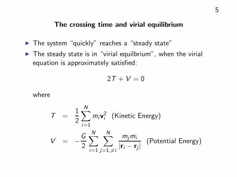
The crossing time and virial equilibrium
◮ The system “quickly” reaches a “steady state”
◮ The steady state is in “virial equilbrium”, when the virialequation is approximately satisfied:
2T + V = 0
where
T =1
2
N∑
i=1
miv2
i (Kinetic Energy)
V = −G
2
N∑
i=1
N∑
j=1, 6=i
mjmi
|ri − rj |(Potential Energy)

6
Mass, length and time scales
◮ Total mass
M =
N∑
i=1
mi
◮ Characterise system size by “virial radius” R defined by
V = −GM2
2R, where M is total mass
◮ Characterise speeds by (mass weighted) mean square speed
v2 =2T
M
◮ Define time scale
tcr =2R
v(“Crossing time”)
7
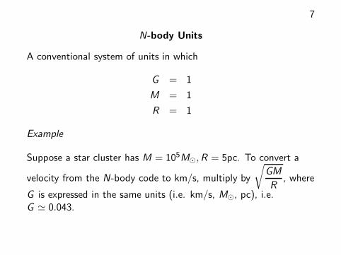
N-body Units
A conventional system of units in which
G = 1
M = 1
R = 1
Example
Suppose a star cluster has M = 105M⊙,R = 5pc. To convert a
velocity from the N-body code to km/s, multiply by
√
GM
R, where
G is expressed in the same units (i.e. km/s, M⊙, pc), i.e.G ≃ 0.043.
8
Significance of the crossing time
◮ Time scale of cold collapse
◮ Time scale of approach to virial equilibrium
◮ Time scale of orbital motions in virial equilibrium
9
Plummer’s model
◮ A particular model of a system in virial (and dynamic)equilibrium
◮ Convenient analytical distributions

10
11
Lessons from the simulations
Evolution on two time scales:
◮ orbital motions (crossing time scale)
◮ much slower evolution of the statistical distribution

12
Two-body relaxation
◮ Local definition tr =0.065v3
ρmG 2 ln γNwhere
◮ v is the velocity dispersion (root mean square velocity)◮ ρ is the space (mass-)density◮ m is the particle mass◮ γ is a constant (about 0.11 for equal masses)◮ N is number of particles
◮ Global definition: half-mass relaxation time
trh = 0.138N1/2r
3/2
h
m1/2G 1/2 ln(γN), where
◮ rh is the half-mass radius (containing the innermost half of thesystem); comparable with the virial radius

13
Significance of the relaxation time
◮ Time scale of core collapse
◮ Time scale of escape (actually several/many tr )
◮ Time scale of mass segregation (if there is a distribution ofmasses, the heavier particles sink to the centre on a time scalewhich is a fraction of tr )
◮ Collisional stellar dynamics deals with phenomena on timescales of a few trh (open and globular star clusters; somegalactic nuclei)
◮ Collisionless stellar dynamics deals with phenomena on timescales much less than trh (spiral structure, galaxy collisions(!), ...)

14
Post-collapse evolution
Depends on boundary conditions:
◮ “isolated” system: binaries form in the core, liberating energy,which expands the system on the time scale trh (by a feedbackmechanism). As rh expands, trh increases. The system very
slowly loses mass
◮ “tidally limited” systems: stars escape (roughly speaking) at atidal radius rt , where external forces become dominant. Massis lost on time scale trh; rt contracts, rh contracts(eventually). System dissolves in few trh.
15
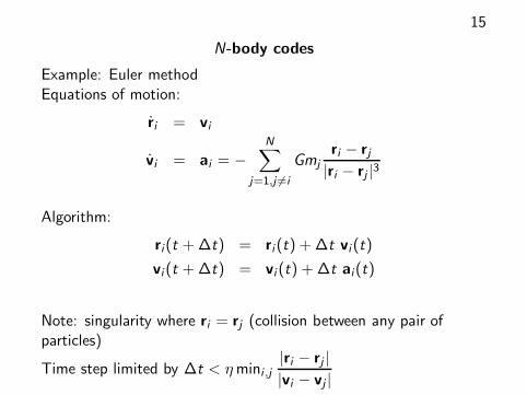
N-body codes
Example: Euler methodEquations of motion:
ri = vi
vi = ai = −
N∑
j=1,j 6=i
Gmj
ri − rj|ri − rj |3
Algorithm:
ri(t + ∆t) = ri (t) + ∆t vi (t)
vi (t + ∆t) = vi (t) + ∆t ai(t)
Note: singularity where ri = rj (collision between any pair ofparticles)
Time step limited by ∆t < η mini ,j|ri − rj |
|vi − vj |
16
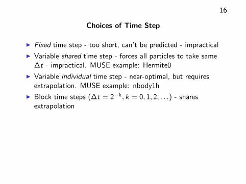
Choices of Time Step
◮ Fixed time step - too short, can’t be predicted - impractical
◮ Variable shared time step - forces all particles to take same∆t - impractical. MUSE example: Hermite0
◮ Variable individual time step - near-optimal, but requiresextrapolation. MUSE example: nbody1h
◮ Block time steps (∆t = 2−k , k = 0, 1, 2, . . .) - sharesextrapolation

17
Conventional choices
Time step: a generalisation of η mini ,j|ri − rj |
|vi − vj |Particle advance: a generalisation of Euler called Hermite
First step:
Euler:ri := ri + vi∆t
vi := vi + ai∆t
Hermite:ri := ri + vi∆t +1
2ai∆t2 +
1
6ai∆t3
vi := vi + ai∆t +1
2ai∆t2
followed by a corrector involving values of ai , ai at the end of thetime step (Hermite only).

18
Basic structure of an N-body code
1. Initialisation of ri , vi , tnexti (update time), ai , ai , all i .
2. Choose i minimising tnexti
3. Extrapolate all rj to tnexti
4. Compute new ai , ai
5. Correct new ri , compute new vi (Hermite integrator)
6. Compute new tnexti
7. Repeat from step 2
Notes
◮ this does not include block time steps
◮ this is the basic structure of NBODY1 (Aarseth)
19
Accelerating force calculation: software
Neighbour Scheme (Ahmad-Cohen)
◮ For each particle i , keep a list of its near neighbours
◮ Update the neighbour force frequently, the non-neighbourforce less frequently (“regular” and “irregular” forces)
Tree code: little used in collisional simulations. MUSE example:BHTree
20
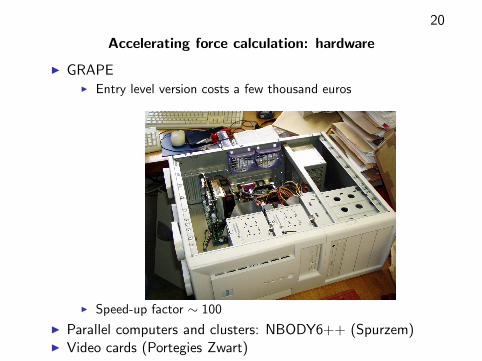
Accelerating force calculation: hardware
◮ GRAPE◮ Entry level version costs a few thousand euros
◮ Speed-up factor ∼ 100
◮ Parallel computers and clusters: NBODY6++ (Spurzem)◮ Video cards (Portegies Zwart)

21
Close encounters and binaries. I. Offset “regularisation”
Suppose particles i , j form a bound pair, or experience a closeencounter. Use offset variables r,R defined as
R =mi ri + mj rj
mi + mj
r = ri − rj ,
and write equations of motion in terms of r,R: e.g.
r = −G (mi + mj)r
|r|3+ a′i − a′j ,
where ′ means we omit force due to i , j .Advantage: avoids rounding error in repeated calculation of ri − rj .

22
Close encounters and binaries. II. KS regularisation
◮ Singularity in
r = −G (mi + mj)r
|r|3+ a′i − a′j
requires small time steps for close and/or eccentric binaries.
◮ KS regularisation is subtle change of variables which removesthe singularity.
◮ still requires short time step for close binary
◮ freeze unperturbed binaries

23
Higher-order subsystems: triples, quadruples, etc
◮ hierarchical triples are binaries constantly perturbed by thirdbody: “slow-down” treatment follows secular perturbationswith (much) larger time step
◮ non-hierarchical triples, quadruples: chain regularisation, ageneralisation of offset and KS regularisation; there arespecilisations to triples and quadruples

24
Flow control
Each integration step may involve any of the following possibilities(Aarseth, NBODY6):
1. Standard integration
2. New KS regularisation
3. KS termination
4. Output
5. 3-body regularisation
6. 4-body regularisation
7. New hierarchical system
8. Termination ofhierarchical system
9. Chain regularisation
10. Physical collisions
Also: stellar evolution

25
N-body codes
1. NBODY1-6 (Aarseth), NBODY6++ (Spurzem): FORTRAN,production code
2. starlab (McMillan, Hut, Makino, Portegies Zwart): C++, noKS regularisation, production code
3. ACS (Hut, Makino): Ruby, experimental
4. MUSE (everyone): Python, FORTRAN, C++, C,experimental; includes a Hermite code, NBODY1h, and aBarnes-Hut tree code

26
Quality control
◮ Energy check
-6e-05
-4e-05
-2e-05
0
2e-05
4e-05
6e-05
8e-05
0 2 4 6 8 10
Ene
rgy
erro
r pe
r ou
tput
tim
e
Time
Cold collapse: N = 1024
◮ Are your answers reasonable?

27
“Complexity”
◮ Effort dominated by calculation of a: N terms
◮ N forces to be calculated
◮ Typical time step ≪ tcr
◮ Typical collisional simulation lasts few tr ∼ Ntcr
Hence effort ∝ N3 at least.
28
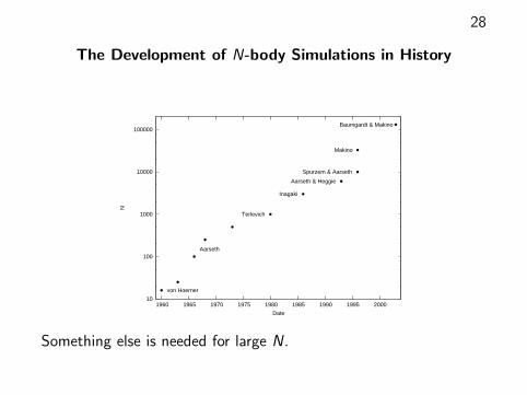
The Development of N-body Simulations in History
10
100
1000
10000
100000
1960 1965 1970 1975 1980 1985 1990 1995 2000
N
Date
von Hoerner
Terlevich
Inagaki
Aarseth & Heggie
Spurzem & Aarseth
Makino
Aarseth
Baumgardt & Makino
Something else is needed for large N.

29
Monte Carlo codes
Assume
◮ Spherical symmetry
◮ Dynamic equilibrium
In a given potential, each particle characterised by
◮ energy E
◮ angular momentum L
These evolve on a time scale of tr . Choose time step = ηtrh.

30
A Monte Carlo Algorithm
1. Initialise positions and velocities, compute Ei ,Li
2. Order the particles by radius, and compute gravitationalpotential φ (easy in spherical symmetry)
3. For each successive pair i , i + 1 compute the local value of tr ,and let i , i + 1 have a two-body encounter yielding, onaverage, the correct effect of two-body relaxation in the timeinterval ∆t.
4. Calculate new E ,L for all particles
5. Reassign radii of all particles (according to the time spent ateach radius given E ,L, φ)
6. Repeat from 2
31
Refinements to the Monte Carlo Algorithm
◮ Different time steps in different zones
◮ Binaries and their interactions using◮ cross sections (Giersz & Heggie)◮ on-the-fly few-body integrations (Fregeau)
◮ Stellar evolution (e.g. McScatter interface)

32
Recent applications (see talks at Capri)
◮ open cluster M67
◮ globular cluster M4

33
References
◮ Stellar Dynamics
1. Galactic Dynamics James Binney and Scott Tremaine,Princeton University Press, 1988, £38.95, 755 pp.
2. Dynamical Evolution of Globular Clusters Lyman J. Spitzer Jr,Princeton UP, 1988, out of print, 196 pp.
3. The Gravitational Million Body Problem, Douglas Heggie, PietHut; Cambridge UP, 2003, $65.00
◮ N-body codes
1. Gravitational N-body simulations, Sverre J. AarsethCambridge: CUP, 2003, £49, 413pp
2. http://www.ids.ias.edu/∼starlab/ (starlab)3. http://artcompsci.org/ (The Art of Computational Science)4. Henon, M. 1971, The Monte Carlo Method, Ap&SS, 14, 151