STELLAR STRUCTUREAND EVOLUTION

O.R. Pols

Astronomical Institute UtrechtSeptember 2011

Preface

These lecture notes are intended for an advanced astrophysics course on Stellar Structure and Evolu-tion given at Utrecht University (NS-AP434M). Their goal is to providean overview of the physicsof stellar interiors and its application to the theory of stellar structure and evolution, at a level appro-priate for a third-year Bachelor student or beginning Master student in astronomy. To a large extentthese notes draw on the classical textbook by Kippenhahn & Weigert (1990; see below), but leavingout unnecessary detail while incorporating recent astrophysical insights and up-to-date results. Atthe same time I have aimed to concentrate on physical insight rather than rigorous derivations, andto present the material in a logical order, following in part the very lucid butsomewhat more basictextbook by Prialnik (2000). Finally, I have borrowed some ideas from thetextbooks by Hansen,Kawaler & Trimble (2004), Salaris & Cassissi (2005) and the recent book by Maeder (2009).

These lecture notes are evolving and I try to keep them up to date. If you find any errors or incon-sistencies, I would be grateful if you could notify me by email (O.R.Pols@uu.nl).

Onno PolsUtrecht, September 2011

Literature

• C.J. Hansen, S.D. Kawaler & V. Trimble,Stellar Interiors, 2004, Springer-Verlag, ISBN 0-387-20089-4 (Hansen)

• R. Kippenhahn & A. Weigert,Stellar Structure and Evolution, 1990, Springer-Verlag, ISBN3-540-50211-4 (Kippenhahn; K&W)

• A. Maeder,Physics, Formation and Evolution of Rotating Stars, 2009, Springer-Verlag, ISBN978-3-540-76948-4 (Maeder)

• D. Prialnik,An Introduction to the Theory of Stellar Structure and Evolution, 2nd edition, 2009,Cambridge University Press, ISBN 0-521-86604-9 (Prialnik)

• M. Salaris & S. Cassisi,Evolution of Stars and Stellar Populations, 2005, John Wiley & Sons,ISBN 0-470-09220-3 (Salaris)

iii

Physical and astronomical constants

Table 1. Physical constants in cgs units (CODATA 2006).

gravitational constant G 6.674 3× 10−8 cm3 g−1 s−2

speed of light in vacuum c 2.997 924 58× 1010 cm s−1

Planck constant h 6.626 069× 10−27 erg sradiation density constant a 7.565 78× 10−15 erg cm−3 K−4

Stefan-Boltzmann constantσ = 14ac 5.670 40× 10−5 erg cm−2 s−1 K−4

Boltzmann constant k 1.380 650× 10−16 erg K−1

Avogadro’s number NA = 1/mu 6.022 142× 1023 g−1

gas constant R = kNA 8.314 47× 107 erg g−1 K−1

electron volt eV 1.602 176 5× 10−12 ergelectron charge e 4.803 26× 10−10 esu

e2 1.440 00× 10−7 eV cmelectron mass me 9.109 382× 10−28 gatomic mass unit mu 1.660 538 8× 10−24 gproton mass mp 1.672 621 6× 10−24 gneutron mass mn 1.674 927 2× 10−24 gα-particle mass mα 6.644 656 2× 10−24 g

Table 2. Astronomical constants, mostly from the Astronomical Almanac (2008).

Solar mass M⊙ 1.988 4× 1033 gGM⊙ 1.327 124 42× 1026 cm3 s−2

Solar radius R⊙ 6.957× 1010 cmSolar luminosity L⊙ 3.842× 1033 erg s−1

year yr 3.155 76× 107 sastronomical unit AU 1.495 978 71× 1013 cmparsec pc 3.085 678× 1018 cm

iv

Chapter 1

Introduction

This introductory chapter sets the stage for the course, and briefly repeats some concepts from earliercourses on stellar astrophysics (e.g. the Utrecht first-year courseIntroduction to stellar structure andevolutionby F. Verbunt).

Thegoalof this course on stellar evolution can be formulated as follows:

to understand the structure and evolution of stars, and their observational properties,using known laws of physics

This involves applying and combining ‘familiar’ physics from many different areas (e.g. thermody-namics, nuclear physics) under extreme circumstances (high temperature,high density), which is partof what makes studying stellar evolution so fascinating.

What exactly do we mean by a ‘star’? A useful definition for the purpose of this course is as follows:a star is an object that (1) radiates energy from an internal source and(2) is bound by its own gravity.This definition excludes objects like planets and comets, because they do notcomply with the firstcriterion. In the strictest sense it also excludes brown dwarfs, which are not hot enough for nuclearfusion, although we will briefly discuss these objects. (The second criterion excludes trivial objectsthat radiate, e.g. glowing coals).

An important implication of this definition is that stars mustevolve(why?). A star is born out of aninterstellar (molecular) gas cloud, lives for a certain amount of time on its internal energy supply, andeventually dies when this supply is exhausted. As we shall see, a second implication of the definitionis that stars can have only a limited range of masses, between∼0.1 and∼100 times the mass of theSun. Thelife and deathof stars forms the subject matter of this course. We will only briefly touch onthe topic ofstar formation, a complex and much less understood process in which the problems to besolved are mostly very different than in the study of stellar evolution.

1.1 Observational constraints

Fundamental properties of a star include themass M(usually expressed in units of the solar mass,M⊙ = 1.99× 1033 g), theradius R(often expressed inR⊙ = 6.96× 1010 cm) and theluminosity L,the rate at which the star radiates energy into space (often expressed inL⊙ = 3.84× 1033 erg/s). Theeffective temperature Teff is defined as the temperature of a black body with the same energy fluxat the surface of the star, and is a good measure for the temperature of thephotosphere. From thedefinition of effective temperature it follows that

L = 4πR2σT4eff . (1.1)

1

In addition, we would like to know thechemical compositionof a star. Stellar compositions areusually expressed as mass fractionsXi , wherei denotes a certain element. This is often simplifiedto specifying the mass fractionsX (of hydrogen),Y (of helium) andZ (of all heavier elements or‘metals’), which add up to unity. Another fundamental property is therotation rateof a star, expressedeither in terms of the rotation periodProt or the equatorial rotation velocityυeq.

Astronomical observations can yield information about these fundamental stellar quantities:

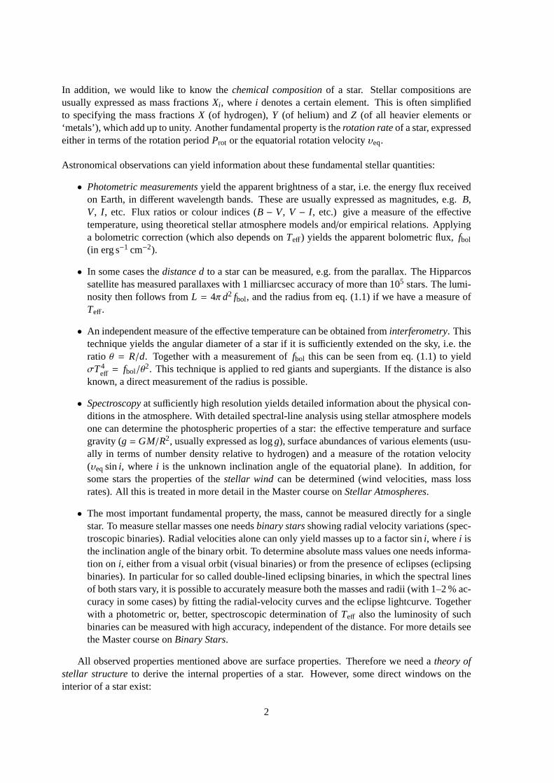
• Photometric measurementsyield the apparent brightness of a star, i.e. the energy flux receivedon Earth, in different wavelength bands. These are usually expressed as magnitudes,e.g. B,V, I , etc. Flux ratios or colour indices (B − V, V − I , etc.) give a measure of the effectivetemperature, using theoretical stellar atmosphere models and/or empirical relations. Applyinga bolometric correction (which also depends onTeff) yields the apparent bolometric flux,fbol

(in erg s−1 cm−2).

• In some cases thedistance dto a star can be measured, e.g. from the parallax. The Hipparcossatellite has measured parallaxes with 1 milliarcsec accuracy of more than 105 stars. The lumi-nosity then follows fromL = 4πd2 fbol, and the radius from eq. (1.1) if we have a measure ofTeff.

• An independent measure of the effective temperature can be obtained frominterferometry. Thistechnique yields the angular diameter of a star if it is sufficiently extended on the sky, i.e. theratio θ = R/d. Together with a measurement offbol this can be seen from eq. (1.1) to yieldσT4

eff = fbol/θ2. This technique is applied to red giants and supergiants. If the distance is also

known, a direct measurement of the radius is possible.

• Spectroscopyat sufficiently high resolution yields detailed information about the physical con-ditions in the atmosphere. With detailed spectral-line analysis using stellar atmosphere modelsone can determine the photospheric properties of a star: the effective temperature and surfacegravity (g = GM/R2, usually expressed as logg), surface abundances of various elements (usu-ally in terms of number density relative to hydrogen) and a measure of the rotation velocity(υeqsini, wherei is the unknown inclination angle of the equatorial plane). In addition, forsome stars the properties of thestellar wind can be determined (wind velocities, mass lossrates). All this is treated in more detail in the Master course onStellar Atmospheres.

• The most important fundamental property, the mass, cannot be measured directly for a singlestar. To measure stellar masses one needsbinary starsshowing radial velocity variations (spec-troscopic binaries). Radial velocities alone can only yield masses up to a factor sini, wherei isthe inclination angle of the binary orbit. To determine absolute mass values one needs informa-tion on i, either from a visual orbit (visual binaries) or from the presence of eclipses (eclipsingbinaries). In particular for so called double-lined eclipsing binaries, in which the spectral linesof both stars vary, it is possible to accurately measure both the masses and radii (with 1–2 % ac-curacy in some cases) by fitting the radial-velocity curves and the eclipse lightcurve. Togetherwith a photometric or, better, spectroscopic determination ofTeff also the luminosity of suchbinaries can be measured with high accuracy, independent of the distance. For more details seethe Master course onBinary Stars.

All observed properties mentioned above are surface properties. Therefore we need atheory ofstellar structureto derive the internal properties of a star. However, some direct windows on theinterior of a star exist:

2

Figure 1.1. H-R diagram of solar neighbourhood. Source: Hipparcos, stars with d measured to< 10 %accuracy.

• neutrinos, which escape from the interior without interaction. So far, the Sun is the only (non-exploding) star from which neutrinos have been detected.

• oscillations, i.e. stellar seismology. Many stars oscillate, and their frequency spectrumcontainsinformation about the speed of sound waves inside the star, and therefore about the interiordensity and temperature profiles. This technique has provided accurate constraints on detailedstructure models for the Sun, and is now also being applied to other stars.

The timespan of any observations is much smaller than a stellar lifetime: observations are likesnapshots in the life of a star. The observed properties of an individualstar contain no (direct) infor-mation about its evolution. The diversity of stellar properties (radii, luminosities, surface abundances)does, however, depend on how stars evolve, as well as on intrinsic properties (mass, initial composi-tion). Properties that are common to a large number of stars must correspondto long-lived evolutionphases, and vice versa. By studying samples of stars statistically we can infer the (relative) lifetimesof certain phases, which provides another important constraint on the theory of stellar evolution.

Furthermore, observations of samples of stars reveal certain correlations between stellar propertiesthat the theory of stellar evolution must explain. Most important are relations between luminosity andeffective temperature, as revealed by theHertzsprung-Russell diagram, and relations between mass,luminosity and radius.

1.1.1 The Hertzsprung-Russell diagram

The Hertzsprung-Russell diagram (HRD) is an important tool to test the theory of stellar evolution.Fig. 1.1 shows the colour-magnitude diagram (CMD) of stars in the vicinity of the Sun, for which theHipparcos satellite has measured accurate distances. This is an example of avolume-limitedsample

3

Figure 1.2. Colour-magnitude diagrams of a young open cluster, M45 (thePleiades, left panel), and a globularcluster, M3 (right panel).

of stars. In this observers’ HRD, the absolute visual magnitudeMV is used as a measure of theluminosity and a colour index (B− V or V − I ) as a measure for the effective temperature. It is leftas an exercise to identify various types of stars and evolution phases in thisHRD, such as the mainsequence, red giants, the horizontal branch, white dwarfs, etc.

Star clusters provide an even cleaner test of stellar evolution. The stars ina cluster were formedwithin a short period of time (a few Myr) out of the same molecular cloud and therefore share the sameage and (initial) chemical composition.1 Therefore, to first-order approximation only the mass variesfrom star to star. A few examples of cluster CMDs are given in Fig. 1.2, fora young open cluster (thePleiades) and an old globular cluster (M3). As the cluster age increases,the most luminous main-sequence stars disappear and a prominent red giant branch and horizontal branch appear. To explainthe morphology of cluster HRDs at different ages is one of the goals of studying stellar evolution.

1.1.2 The mass-luminosity and mass-radius relations

For stars with measured masses, radii and luminosities (i.e. binary stars) we can plot these quantitiesagainst each other. This is done in Fig. 1.3 for the components of double-lined eclipsing binaries forwhich M, R andL are all measured with∼< 2 % accuracy. These quantities are clearly correlated, andespecially the relation between mass and luminosity is very tight. Most of the starsin Fig. 1.3 arelong-lived main-sequence stars; the spread in radii for masses between1 and 2M⊙ results from thefact that several more evolved stars in this mass range also satisfy the 2 % accuracy criterion. Theobserved relations can be approximated reasonably well by power laws:

L ∝ M3.8 and R∝ M0.7. (1.2)

Again, the theory of stellar evolution must explain the existence and slopes ofthese relations.

1The stars in a cluster thus consitute a so-calledsimple stellar population. Recently, this simple picture has changedsomewhat after the discovery of multiple populations in many star clusters.

4

−1 0 1

−2

0

2

4

6

log (M / Msun)

log

(L /

L sun

)

−1 0 1−1.0

−0.5

0.0

0.5

1.0

log (M / Msun)

log

(R /

R sun

)Figure 1.3. Mass-luminosity (left) and mass-radius (right) relationsfor components of double-lined eclipsingbinaries with accurately measuredM, RandL.

1.2 Stellar populations

Stars in the Galaxy are divided into different populations:

• Population I: stars in the galactic disk, in spiral arms and in (relatively young) open clusters.These stars have ages∼< 109 yr and are relatively metal-rich (Z ∼ 0.5− 1Z⊙)

• Population II: stars in the galactic halo and in globular clusters, with ages∼ 1010 yr. These starsare observed to be metal-poor (Z ∼ 0.01− 0.1Z⊙).

An intermediate population (with intermediate ages and metallicities) is also seen in the disk of theGalaxy. Together they provide evidence for thechemical evolutionof the Galaxy: the abundanceof heavy elements (Z) apparently increases with time. This is the result of chemical enrichment bysubsequent stellar generations.

The study of chemical evolution has led to the hypothesis of a ‘Population III’ consisting of thefirst generation of stars formed after the Big Bang, containing only hydrogen and helium and noheavier elements (‘metal-free’,Z = 0). No metal-free stars have ever been observed, probably due tothe fact that they were massive and had short lifetimes and quickly enriched the Universe with metals.However, a quest for finding their remnants has turned up many very metal-poor stars in the halo,with the current record-holder having an iron abundanceXFe = 4× 10−6XFe,⊙.

1.3 Basic assumptions

We wish to build a theory of stellar evolution to explain the observational constraints highlightedabove. In order to do so we must make some basic assumptions:

• stars are considered to beisolatedin space, so that their structure and evolution depend only onintrinsic properties (mass and composition). For most single stars in the Galaxy this conditionis satisfied to a high degree (compare for instance the radius of the Sun with the distance to its

5

nearest neighbour Proxima Centauri, see exercise 1.2). However, for stars in dense clusters, orin binary systems, the evolution can be influenced by interaction with neighbouring stars. Inthis course we will mostly ignore these complicating effects (many of which are treated in theMaster course onBinary Stars).

• stars are formed with ahomogeneous composition, a reasonable assumption since the molecularclouds out of which they form are well-mixed. We will often assume a so-called ‘quasi-solar’composition (X = 0.70, Y = 0.28 andZ = 0.02), even though recent determinations of solarabundances have revised the solar metallicity down toZ = 0.014. In practice there is relativelylittle variation in composition from star to star, so that the initial mass is the most importantparameter that determines the evolution of a star. The composition, in particularthe metallicityZ, is of secondary influence but can have important effects especially in very metal-poor stars(see§ 1.2).

• spherical symmetry, which is promoted by self-gravity and is a good approximation for moststars. Deviations from spherical symmetry can arise if non-central forces become importantrelative to gravity, in particular rotation and magnetic fields. Although many stars are observedto have magnetic fields, the field strength (even in highly magnetized neutron stars) is alwaysnegligible compared to gravity. Rotation can be more important, and therotation ratecan beconsidered an additional parameter (besides mass and composition) determining the structureand evolution of a star. For the majority of stars (e.g. the Sun) the forces involved are smallcompared to gravity. However, some rapidly rotating stars are seen (by means of interferome-try) to be substantially flattened.

1.4 Aims and overview of the course

In the remainder of this course we will:

• understand the global properties of stars: energetics and timescales

• study the micro-physics relevant for stars: the equation of state, nuclearreactions, energy trans-port and opacity

• derive the equations necessary to model the internal structure of stars

• examine (quantitatively) the properties of simplified stellar models

• survey (mostly qualitatively) how stars of different masses evolve, and the endpoints of stellarevolution (white dwarfs, neutron stars)

• discuss a few ongoing research areas in stellar evolution

Suggestions for further reading

The contents of this introductory chapter are also largely covered by Chapter 1 of Prialnik, whichprovides nice reading.

6

Exercises

1.1 Evolutionary stages

In this course we use many concepts introduced in the introductory astronomy classes. In this exercisewe recapitulate the names of evolutionary phases. During the lectures you are assumed to be familiarwith these terms, in the sense that you are able to explain them in general terms.

We encourage you to use Carroll & Ostlie, Introduction to Modern Astrophysics, or the book of thefirst year course (Verbunt, Het leven van sterren) to make a list of the concepts printed initalic with abrief explanation in your own words.

(a) Figure 1.1 shows the location of stars in the solar neighborhood in the Hertzsprung-Russel dia-gram. Indicate in Figure 1.1 where you would find:

main-sequence stars, neutron stars,the Sun, black holes,red giants, binary stars,horizontal branch stars, planets,asymptotic giant branch (AGB) stars, pre-main sequence stars,centrals star of planetary nebulae, hydrogen burning stars,white dwarfs, helium burning stars.

(b) Through which stages listed above will the Sun evolve? Put them in chronological order. Throughwhich stages will a massive star evolve?

(c) Describe the following concepts briefly in your own words. You will need the concepts indicatedwith * in the coming lectures.

ideal gas*, Jeans mass,black body, Schwarzschild criterion,virial theorem*, energy transport by radiation,first law of thermodynamics*, energy transport by convection,equation of state, pp-chain,binary stars, CNO cycle,star cluster, nuclear timescale*,interstellar medium, thermal or Kelvin-Helmholtz timescale*,giant molecular clouds, dynamical timescale*

1.2 Basic assumptions

Let us examine the three basic assumptions made in the theoryof stellar evolution:

(a) Stars are assumed to be isolated in space.The star closest to the sun, Proxima Centauri, is 4.3light-years away. How many solar radii is that? By what factors are the gravitational field andthe radiation flux diminished? Many stars are formed in clusters and binaries. How could thatinfluence the life of a star?

(b) Stars are assumed to form with a uniform composition.What elements is the Sun made of? Justafter the Big Bang the Universe consisted almost purely of hydrogen and helium. Where do allthe heavier elements come from?

(c) Stars are assumed to be spherically symmetric.Why are stars spherically symmetric to a goodapproximation? How would rotation affect the structure and evolution of a star? The Sun rotatesaround its axis every 27 days. Calculate the ratio of is the centrifugal accelerationa over thegravitational accelerationg for a mass element on the surface of the Sun. Does rotation influencethe structure of the Sun?

1.3 Mass-luminosity and mass-radius relation

(a) The masses of stars are approximately in the range 0.08M⊙ . M . 100M⊙. Why is there anupper limit? Why is there a lower limit?

7

(b) Can you think of methods to measure (1) the mass, (2) the radius, and (3) the luminosity of astar? Can your methods be applied for any star or do they require special conditions. Discuss yourmethods with your fellow students.

(c) Figure 1.3 shows the luminosity versus the mass (left) and the radius versus the mass (right) forobserved main sequence stars. We can approximate a mass-luminosity and mass-radius relationby fitting functions of the form

LL⊙=

(

MM⊙

)x

,RL⊙=

(

MM⊙

)y

(1.3)

Estimatex andy from Figure 1.3.

(d) Which stars live longer, high mass stars (which have more fuel) or low mass stars? Derive anexpression for the lifetime of a star as a function of its mass. (!)

[Hints: Stars spend almost all their life on the main sequence burning hydrogen until they runout of fuel. First try to estimate the life time as function ofthe mass (amount of fuel) and theluminosity (rate at which the fuel is burned).]

1.4 The ages of star clusters

Figure 1.4. H-R diagrams of three star clusters (from Prialnik).

The stars in a star cluster are formed more or less simultaneously by fragmentation of a large moleculargas cloud.

(a) In Fig. 1.4 the H-R diagrams are plotted of the stars in three different clusters. Which cluster isthe youngest?

(b) Think of a method to estimate the age of the clusters, discuss with your fellow students. Estimatethe ages and compare with the results of your fellow students.

(c) (*) Can you give an error range on your age estimates?

8

Chapter 2

Mechanical and thermal equilibrium

In this chapter we apply the physical principles of mass conservation and momentum conservation toderive two of the fundamental stellar structure equations. We shall see that stars are generally in astate of almost completemechanical equilibrium, which allows us to derive and apply the importantvirial theorem. We consider the basic stellar timescales and see that most (but not all) starsare alsoin a state of energy balance calledthermal equilibrium.

2.1 Coordinate systems and the mass distribution

The assumption of spherical symmetry implies that all interior physical quantities(such as densityρ,pressureP, temperatureT, etc) depend only on one radial coordinate. The obvious coordinate to usein a Eulerian coordinate system is the radius of a spherical shell,r (∈ 0 . . .R). In an evolving star,all quantities also depend on timet. When constructing the differential equations for stellar structureone should thus generally consider partial derivatives of physical quantities with respect to radius andtime,∂/∂r and∂/∂t, taken at constantt andr, respectively.

The principle of mass conservation applied to the mass dm of a spherical shell of thickness dr atradiusr (see Fig. 2.1) gives

dm(r, t) = 4πr2 ρ dr − 4πr2 ρ υdt, (2.1)

whereυ is the radial velocity of the mass shell. Therefore one has

∂m∂r= 4πr2 ρ and

∂m∂t= −4πr2 ρ υ. (2.2)

The first of these partial differential equations relates the radial mass distribution in the star to thelocal density: it constitutes the first fundamental equation of stellar structure. Note thatρ = ρ(r, t)is not known a priori, and must follow from other conditions and equations. The second equation of(2.2) represents the change of mass inside a sphere of radiusr due to the motion of matter throughits surface; at the stellar surface this gives the mass-loss rate (if there is astellar wind withυ > 0) ormass-accretion rate (if there is inflow withυ < 0). In a static situation, where the velocity is zero, thefirst equation of (2.2) becomes an ordinary differential equation,

dmdr= 4πr2 ρ. (2.3)

This is almost always a good approximation for stellar interiors, as we shall see. Integration yieldsthe massm(r) inside a spherical shell of radiusr:

m(r) =∫ r

04πr ′2ρ dr ′.

9

m

m+dm

dm

F

r

gP(r)

P(r+dr)

dr

dS

Figure 2.1. Mass shell inside a spherically symmetricstar, at radiusr and with thickness dr. The mass of theshell is dm = 4πr2ρdr. The pressure and the gravita-tional force acting on a cylindrical mass element arealso indicated.

Sincem(r) increases monotonically outward, we can also usem(r) as our radial coordinate, insteadof r. Thismass coordinate, often denoted asmr or simplym, is a Lagrangian coordinate that moveswith the mass shells:

m := mr =

∫ r

04πr ′2ρ dr ′ (m ∈ 0 . . .M). (2.4)

It is often more convenient to use a Lagrangian coordinate instead of a Eulerian coordinate. The masscoordinate is defined on a fixed interval,m ∈ 0 . . .M, as long as the star does not lose mass. On theother handr depends on the time-varying stellar radiusR. Furthermore the mass coordinate followsthe mass elements in the star, which simplifies many of the time derivatives that appear in the stellarevolution equations (e.g. equations for the composition). We can thus write allquantities as functionsof m, i.e. r = r(m), ρ = ρ(m), P = P(m), etc.

Using the coordinate transformationr → m, i.e.

∂

∂m=∂

∂r· ∂r∂m

, (2.5)

the first equation of stellar structure becomes in terms of the coordinatem:

∂r∂m=

14πr2ρ

(2.6)

which again becomes an ordinary differential equation in a static situation.

2.1.1 The gravitational field

Recall that a star is a self-gravitating body of gas, which implies that gravity isthe driving forcebehind stellar evolution. In the general, non-spherical case, the gravitational accelerationg can bewritten as the gradient of the gravitational potential,g = −∇Φ, whereΦ is the solution of the Poissonequation

∇2Φ = 4πGρ.

Inside a spherically symmetric body, this reduces tog := |g| = dΦ/dr. The gravitational accelerationat radiusr and equivalent mass coordinatem is then given by

g =Gm

r2. (2.7)

10

Spherical shells outsider apply no net force, so thatg only depends on the mass distribution insidethe shell at radiusr. Note thatg is the magnitude of the vectorg which points inward (toward smallerr or m).

2.2 The equation of motion and hydrostatic equilibrium

We next consider conservation of momentum inside a star, i.e. Newton’s second law of mechanics.The net acceleration on a gas element is determined by the sum of all forcesacting on it. In addition tothe gravitational force considered above, forces result from the pressure exerted by the gas surround-ing the element. Due to spherical symmetry, the pressure forces acting horizontally (perpendicular tothe radial direction) balance each other and only the pressure forces acting along the radial directionneed to be considered. By assumption we ignore other forces that might act inside a star (Sect. 1.3).

Hence the net acceleration ¨r = ∂2r/∂t2 of a (cylindrical) gas element with mass

dm= ρ dr dS (2.8)

(where dr is its radial extent and dS is its horizontal surface area, see Fig. 2.1) is given by

r dm= −gdm+ P(r) dS − P(r + dr) dS. (2.9)

We can writeP(r + dr) = P(r) + (∂P/∂r) · dr, hence after substituting eqs. (2.7) and (2.8) we obtaintheequation of motionfor a gas element inside the star:

∂2r

∂t2= −Gm

r2− 1ρ

∂P∂r. (2.10)

This is a simplified from of the Navier-Stokes equation of hydrodynamics, applied to spherical sym-metry (see Maeder). Writing the pressure gradient∂P/∂r in terms of the mass coordinatem bysubstituting eq. (2.6), the equation of motion is

∂2r

∂t2= −Gm

r2− 4πr2 ∂P

∂m. (2.11)

Hydrostatic equilibrium The great majority of stars are obviously in such long-lived phases ofevolution that no change can be observed over human lifetimes. This means there is no noticeableacceleration, and all forces acting on a gas element inside the star almost exactly balance each other.Thus most stars are in a state of mechanical equilibrium which is more commonly called hydrostaticequilibrium(HE).

The state of hydrostatic equilibrium, setting ¨r = 0 in eq. (2.10), yields the second differentialequation of stellar structure:

dPdr= −Gm

r2ρ, (2.12)

or with eq. (2.6)

dPdm= − Gm

4πr4(2.13)

A direct consequence is that inside a star in hydrostatic equilibrium, the pressure always decreasesoutwards.

Eqs. (2.6) and (2.13) together determine themechanical structureof a star in HE. These aretwo equations for three unknown functions ofm (r, P andρ), so they cannot be solved without a

11

third condition. This condition is usually a relation betweenP andρ called theequation of state(see Chapter 3). In general the equation of state depends on the temperature T as well, so that themechanical structure depends also on the temperature distribution inside the star, i.e. on its thermalstructure. In special cases the equation of state is independent ofT, and can be written asP =P(ρ). In such cases (known as barotropes or polytropes) the mechanicalstructure of a star becomesindependent of its thermal structure. This is the case for white dwarfs, aswe shall see later.

Estimates of the central pressure A rough order-of-magnitude estimate of the central pressure canbe obtained from eq. (2.13) by setting

dPdm∼ Psurf − Pc

M≈ −Pc

M, m∼ 1

2M, r ∼ 12R

which yields

Pc ∼2π

GM2

R4(2.14)

For the Sun we obtain from this estimatePc ∼ 7× 1015 dyn/cm2 = 7× 109 atm.A lower limit on the central pressure may be derived by writing eq. (2.13) as

dPdr= − Gm

4πr4

dmdr= − d

dr

(

Gm2

8πr4

)

− Gm2

2πr5,

and thus

ddr

(

P+Gm2

8πr4

)

= −Gm2

2πr5< 0. (2.15)

The quantityΨ(r) = P+Gm2/(8πr4) is therefore a decreasing function ofr. At the centre, the secondterm vanishes becausem ∝ r3 for small r, and henceΨ(0) = Pc. At the surface, the pressure isessentially zero. From the fact thatΨmust decrease withr it thus follows that

Pc >18π

GM2

R4. (2.16)

In contrast to eq. (2.14), this is a strict mathematical result, valid for any starin hydrostatic equilibriumregardless of its other properties (in particular, regardless of its densitydistribution). For the Sun weobtainPc > 4.4 × 1014 dyn/cm2. Both estimates indicate that an extremely high central pressure isrequired to keep the Sun in hydrostatic equilibrium. Realistic solar models show the central densityto be 2.4× 1017 dyn/cm2.

2.2.1 The dynamical timescale

We can ask what happens if the state of hydrostatic equilibrium is violated: how fast do changesto the structure of a star occur? The answer is provided by the equation ofmotion, eq. (2.10). Forexample, suppose that the pressure gradient that supports the star against gravity suddenly drops. Allmass shells are then accelerated inwards by gravity: the star starts to collapse in “free fall”. We canapproximate the resulting (inward) acceleration by

|r | ≈ R

τff2⇒ τff ≈

√

R|r |

12

whereτff is the free-fall timescale that we want to determine. Since−r = g ≈ GM/R2 for the entirestar, we obtain

τff ≈

√

Rg≈

√

R3

GM. (2.17)

Of course each mass shell is accelerated at a different rate, so this estimate should be seen as anaverage value for the star to collapse over a distanceR. This provides one possible estimate for thedynamical timescaleof the star. Another estimate can be obtained in a similar way by assuming thatgravity suddenly disappears: this gives the timescale for the outward pressure gradient to explode thestar, which is similar to the time it takes for a sound wave to travel from the centreto the surface ofthe star. If the star is close to HE, all these timescales have about the same value given by eq. (2.17).Since the average density ¯ρ = 3M/(4πR3), we can also write this (hydro)dynamical timescale as

τdyn ≈√

R3

GM≈ 1

2 (Gρ)−1/2. (2.18)

For the Sun we obtain a very small value ofτdyn ≈ 1600 sec or about half an hour (0.02 days). Thisis very much smaller than the age of the Sun, which is 4.6 Gyr or∼ 1.5 × 1017 sec, by 14 orders ofmagnitude. This result has several important consequences for the Sunand other stars:

• Any significant departure from hydrostatic equilibrium should very quickly lead to observablephenomena: either contraction or expansion on the dynamical timescale. If the star cannotrecover from this disequilibrium by restoring HE, it should lead to a collapseor an explosion.

• Normally hydrostatic equilibrium can be restored after a disturbance (we willconsider thisdynamical stabilityof stars later). However a perturbation of HE may lead to small-scale oscil-lations on the dynamical timescale. These are indeed observed in the Sun andmany other stars,with a period of minutes in the case of the Sun. Eq. (2.18) tells us that the pulsation period is a(rough) measure of the average density of the star.

• Apart from possible oscillations, stars are extremely close to hydrostatic equilibrium, sinceany disturbance is immediately quenched. We can therefore be confident that eq. (2.13) holdsthroughout most of their lifetimes. Stars do evolve and are therefore not completely static, butchanges occur very slowly compared to their dynamical timescale. Stars canbe said to evolvequasi-statically, i.e. through a series of near-perfect HE states.

2.3 The virial theorem

An important consequence of hydrostatic equilibrium is thevirial theorem, which is of vital impor-tance for the understanding of stars. It connects two important energy reservoirs of a star and allowspredictions and interpretations of important phases in the evolution of stars.

To derive the virial theorem we start with the equation for hydrostatic equilibrium eq. (2.13). Wemultiply both sides by the enclosed volumeV = 4

3πr3 and integrate overm:∫ M

0

43πr3 dP

dmdm= −1

3

∫ M

0

Gmr

dm (2.19)

The integral on the right-hand side has a straightforward physical interpretation: it is thegravitationalpotential energyof the star. To see this, consider the work done by the gravitational forceF to bringa mass elementδm from infinity to radiusr:

δW =∫ r

∞F · dr =

∫ r

∞

Gmδm

r2dr = −GM

rδm.

13

The gravitational potential energy of the star is the work performed by the gravitational force to bringall mass elements from infinity to their current radius, i.e.

Egr = −∫ M

0

Gmr

dm (2.20)

The left-hand side of eq. (2.19) can be integrated by parts:∫ Ps

Pc

V dP = [V · P]sc −

∫ Vs

0PdV (2.21)

wherec ands denote central and surface values. Combining the above expressions ineq. (2.19) weobtain

43πR3 P(R) −

∫ Vs

0PdV = 1

3Egr, (2.22)

with P(R) the pressure at the surface of the volume. This expression is useful when the pressure fromthe surrounding layers is substantial, e.g. when we consider only the coreof a star. If we considerthe star as a whole, however, the first term vanishes because the pressure at the stellar surface isnegligible. In that case

−3∫ Vs

0PdV = Egr, (2.23)

or, since dV = dm/ρ,

−3∫ M

0

Pρ

dm= Egr. (2.24)

This is the general form of the virial theorem, which will prove valuable later. It tells us that that theaverage pressure needed to support a star in HE is equal to−1

3Egr/V. In particular it tells us that astar that contracts quasi-statically (that is, slowly enough to remain in HE) must increase its internalpressure, since|Egr| increases while its volume decreases.

The virial theorem for an ideal gas The pressure of a gas is related to its internal energy. We willshow this in Ch. 3, but for the particular case of an ideal monatomic gas it is easy to see. The pressureof an ideal gas is given by

P = nkT =ρ

µmukT, (2.25)

wheren = N/V is the number of particles per unit volume, andµ is mass of a gas particle in atomicmass units. The kinetic energy per particle isǫk =

32kT, and the internal energy of an ideal monatomic

gas is equal to the kinetic energy of its particles. The internal energy per unit mass is then

u =32

kTµmu

=32

Pρ. (2.26)

We can now interpret the left-hand side of the virial theorem (eq. 2.24) as∫

(P/ρ) dm= 23

∫

udm=23Eint, whereEint is the total internal energy of the star. The virial theorem for an ideal gasis therefore

Eint = −12Egr (2.27)

This important relation establishes a link between the gravitational potential energy and the internalenergy of a star in hydrostatic equilibrium that consists of an ideal gas. (We shall see later that theideal gas law indeed holds for most stars, at least on the main sequence.) The virial theorem tellsus that a more tightly bound star must have a higher internal energy, i.e. it mustbehotter. In otherwords, a star that contracts quasi-statically must get hotter in the process.The full implications of thisresult will become clear when we consider the total energy of a star in a short while.

14

Estimate of the central temperature Using the virial theorem we can obtain an estimate of theaverage temperature inside a star composed of ideal gas. The gravitational energy of the star is foundfrom eq. (2.20) and can be written as

Egr = −αGM2

R, (2.28)

whereα is a constant of order unity (determined by the distribution of matter in the star, i.e. bythe density profile). Using eq. (2.26), the internal energy of the star isEint =

32k/(µmu)

∫

Tdm =32k/(µmu)T M, whereT is the temperature averaged over all mass shells. By the virial theorem wethen obtain

T =α

3µmu

kGMR

. (2.29)

Takingα ≈ 1 andµ = 0.5 for ionized hydrogen, we obtain for the SunT ∼ 4 × 106 K. This is theaverage temperature required to provide the pressure that is needed to keep the Sun in hydrostaticequilibrium. Since the temperature in a star normally decreases outwards, it is also an approximatelower limit on the central temperature of the Sun. At these temperatures, hydrogen and helium areindeed completely ionized. We shall see thatTc ≈ 107 K is high enough for hydrogen fusion to takeplace in the central regions of the Sun.

The virial theorem for a general equation of state Also for equations of state other than an idealgas a relation between pressure and internal energy exists, which we can write generally as

u = φPρ. (2.30)

We have seen above thatφ = 32 for an ideal gas, but it will turn out (see Ch. 3) that this is valid not

only for an ideal gas, but for all non-relativistic particles. On the other hand, if we consider a gas ofrelativistic particles, in particular photons (i.e. radiation pressure),φ = 3. If φ is constant throughoutthe star we can integrate the left-hand side of eq. (2.23) to obtain a more general form of the virialtheorem:

Eint = −13φEgr (2.31)

2.3.1 The total energy of a star

The total energy of a star is the sum of its gravitational potential energy, its internal energy and itskinetic energyEkin (due to bulk motions of gas inside the star, not the thermal motions of the gasparticles):

Etot = Egr + Eint + Ekin. (2.32)

The star is bound as long as its total energy is negative.For a star in hydrostatic equilibrium we can setEkin = 0. Furthermore for a star in HE the virial

theorem holds, so thatEgr andEint are tightly related by eq. (2.31). Combining eqs. (2.31) and (2.32)we obtain the following relations:

Etot = Eint + Egr =φ − 3φ

Eint = (1− 13φ)Egr (2.33)

15

As long asφ < 3 the star is bound. This is true in particular for the important case of a star consistingof an ideal gas (eq. 2.27), for which we obtain

Etot = Eint + Egr = − Eint =12Egr < 0 (2.34)

In other words, its total energy of such a star equals half of its gravitational potential energy.From eq. (2.34) we can see that the virial theorem has the following important consequences:

• Gravitationally bound gas spheres must behot to maintain hydrostatic equilibrium: heat pro-vides the pressure required to balance gravity. The more compact such asphere, the morestrongly bound, and therefore the hotter it must be.

• A hot sphere of gas radiates into surrounding space, therefore a starmust lose energy from itssurface. The rate at which energy is radiated from the surface is theluminosityof the star. Inthe absence of an internal energy source, this energy loss must equalthe decrease of the totalenergy of the star:L = −dEtot/dt > 0, sinceL is positive by convention.

• Taking the time derivative of eq. (2.34), we find that as a consequence of losing energy:

Egr = −2L < 0,

meaning that the starcontracts(becomes more strongly bound), and

Eint = L > 0,

meaning that the stargets hotter– unlike familiar objects which cool when they lose energy.Therefore a star can be said to have anegative heat capacity. Half the energy liberated bycontraction is used for heating the star, the other half is radiated away.

For the case of a star that is dominated by radiation pressure, we find thatEint = −Egr, and there-fore the total energyEtot = 0. Therefore a star dominated by radiation pressure (or more generally,by the pressure of relativistic particles) is only marginally bound. No energy is required to expand orcontract such a star, and a small perturbation would be enough to renderit unstable and to trigger itscollapse or complete dispersion.

2.3.2 Thermal equilibrium

If internal energy sources are present in a star due to nuclear reactions taking place in the interior, thenthe energy loss from the surface can be compensated:L = Lnuc ≡ −dEnuc/dt. In that case the totalenergy is conserved and eq. (2.34) tells us thatEtot = Eint = Egr = 0. The virial theorem thereforestates that bothEint andEgr are conserved as well: the star cannot, for example, contract and coolwhile keeping its total energy constant.

In this state, known asthermal equilibrium(TE), the star is in a stationary state. Energy is radiatedaway at the surface at the same rate at which it is produced by nuclear reactions in the interior. Thestar neither expands nor contracts, and it maintains a constant interior temperature. We shall seelater that this temperature is regulated by the nuclear reactions themselves, which in combinationwith the virial theorem act like a stellar thermostat. Main-sequence stars like theSun are in thermalequilibrium, and a star can remain in this state as long as nuclear reactions can supply the necessaryenergy.

16

Note that the arguments given above imply that both hydrostatic equilibrium andthermal equilib-rium arestableequilibria, an assumption that we have yet to prove (see Ch. 7). It is relatively easy tounderstand why TE is stable, at least as long as the ideal-gas pressure dominates (φ < 3 in eq. 2.31).Consider what happens when TE is disturbed, e.g. whenLnuc > L temporarily. The total energy thenincreases, and the virial theorem states that as a consequence the star must expand and cool. Sincethe nuclear reaction rates typically increase strongly with temperature, the rate of nuclear burning andthusLnuc will decrease as a result of this cooling, until TE is restored whenL = Lnuc.

2.4 The timescales of stellar evolution

Three important timescales are relevant for stellar evolution, associated withchanges to the mechani-cal structure of a star (described by the equation of motion, eq. 2.11), changes to its thermal structure(as follows from the virial theorem, see also Sect. 5.1) and changes in its composition, which will bediscussed in Ch. 6.

The first timescale was already treated in Sec. 2.2.1: it is thedynamical timescalegiven byeq. (2.18),

τdyn ≈√

R3

GM≈ 0.02

(

RR⊙

)3/2(M⊙M

)1/2

days (2.35)

The dynamical timescale is the timescale on which a star reacts to a perturbation ofhydrostatic equi-librium. We saw that this timescale is typically of the order of hours or less, whichmeans that starsare extremely close to hydrostatic equilibrium.

2.4.1 The thermal timescale

The second timescale describes how fast changes in the thermal structureof a star can occur. It istherefore also the timescale on which a star in thermal equilibrium reacts when itsTE is perturbed.To obtain an estimate, we turn to the virial theorem: we saw in Sec. 2.3.1 that a starwithout a nuclearenergy source contracts by radiating away its internal energy content:L = Eint ≈ −2Egr, where thelast equality applies strictly only for an ideal gas. We can thus define thethermalor Kelvin-Helmholtztimescaleas the timescale on which this gravitational contraction would occur:

τKH =Eint

L≈|Egr|2L≈ GM2

2RL≈ 1.5× 107

(

MM⊙

)2R⊙R

L⊙L

yr (2.36)

Here we have used eq. (2.28) forEgr with α ≈ 1.The thermal timescale for the Sun is about 1.5 × 107 years, which is many orders of magnitude

larger than the dynamical timescale. There is therefore no direct observational evidence that anystar is in thermal equilibrium. In the late 19th century gravitational contraction was proposed as theenergy source of the Sun by Lord Kelvin and, independently, by Hermann von Helmholtz. This led toan age of the Sun and an upper limit to the age the Earth that was in conflict with emerging geologicalevidence, which required the Earth to be much older. Nuclear reactions have since turned out to bea much more powerful energy source than gravitational contraction, allowing stars to be in thermalequilibrium for most (> 99 %) of their lifetimes. However, several phases of stellar evolution, duringwhich the nuclear power source is absent or inefficient, do occur on the thermal timescale.

17

2.4.2 The nuclear timescale

A star can remain in thermal equilibrium for as long as its nuclear fuel supply lasts. The associatedtimescale is called thenuclear timescale, and since nuclear fuel (say hydrogen) is burned into ‘ash’(say helium), it is also the timescale on which composition changes in the stellar interior occur.

The energy source of nuclear fusion is the direct conversion of a smallfractionφ of the rest massof the reacting nuclei into energy. For hydrogen fusion,φ ≈ 0.007; for fusion of helium and heavierelementsφ is smaller by a factor 10 or more. The total nuclear energy supply can therefore be writtenasEnuc = φMnucc2 = φ fnucMc2, where fnuc is that fraction of the mass of the star which may serve asnuclear fuel. In thermal equilibriumL = Lnuc = Enuc, so we can estimate the nuclear timescale as

τnuc =Enuc

L= φ fnuc

Mc2

L≈ 1010 M

M⊙

L⊙L

yr. (2.37)

The last approximate equality holds for hydrogen fusion in a star like the Sun,with has 70 % of itsinitial mass in hydrogen and fusion occurring only in the inner≈ 10 % of its mass (the latter resultcomes from detailed stellar models). This long timescale is consistent with the geological evidencefor the age of the Earth.

We see that, despite only a small fraction of the mass being available for fusion, the nucleartimescale is indeed two to three orders of magnitude larger than the thermal timescale. Therefore theassumption that stars can reach a state of thermal equilibrium is justified. To summarize, we havefound:

τnuc≫ τKH ≫ τdyn.

As a consequence, the rates of nuclear reactions determine the pace of stellar evolution, and stars maybe assumed to be in hydrostatic and thermal equilibrium throughout most of their lives.

Suggestions for further reading

The contents of this chapter are covered more extensively by Chapter 1 of Maeder and by Chapters 1to 4 of Kippenhahn & Weigert.

Exercises

2.1 Density profile

In a star with massM, assume that the density decreases from the center to the surface as a function ofradial distancer, according to

ρ = ρc

[

1−( rR

)2]

, (2.38)

whereρc is a given constant andR is the radius of the star.

(a) Findm(r).

(b) Derive the relation betweenM andR.

(c) Show that the average density of the star is 0.4ρc.

18

2.2 Hydrostatic equilibrium

(a) Consider an infinitesimal mass element dm inside a star, see Fig. 2.1. What forces act on this masselement?

(b) Newton’s second law of mechanics, or the equation of motion, states that the net force acting ona body is equal to its acceleration times it mass. Write down the equation of motion for the gaselement.

(c) In hydrostatic equilibrium the net force is zero and the gas element is not accelerated. Find anexpression of the pressure gradient in hydrostatic equilibrium.

(d) Find an expression for the central pressurePc by integrating the pressure gradient. Use this toderive the lower limit on the central pressure of a star in hydrostatic equilibrium, eq. (2.16).

(e) Verify the validity of this lower limit for the case of a star with the density profile of eq. (2.38).

2.3 The virial theorem

An important consequence of hydrostatic equilibrium is that it links the gravitational potential energyEgr and the internal thermal energyEint.

(a) Estimate the gravitational energyEgr for a star with massM and radiusR, assuming (1) a constantdensity distribution and (2) the density distribution of eq. (2.38).

(b) Assume that a star is made of an ideal gas. What is the kinetic internal energy per particle for anideal gas? Show that the total internal energy,Eint is given by:

Eint =

∫ R

0

(

32

kµmu

ρ(r)T(r)

)

4πr2 dr. (2.39)

(c) Estimate the internal energy of the Sun by assuming constant density andT(r) ≈ 〈T〉 ≈ 12Tc ≈

5× 106K and compare your answer to your answer for a). What is the totalenergy of the Sun? Isthe Sun bound according to your estimates?

It is no coincidence that the order of magnitude forEgr and Eint are the same1. This follows fromhydrostatic equilibrium and the relation is known as the virial theorem. In the next steps we will derivethe virial theorem starting from the pressure gradient in the form of eq. (2.12).

(d) Multiply by both sides of eq. (2.12) by 4πr3 and integrate over the whole star. Use integration byparts to show that

∫ R

03P 4πr2 dr =

∫ R

0

Gm(r)r

ρ4πr2 dr. (2.40)

(e) Now derive a relation betweenEgr andEint, the virial theorem for an ideal gas.

(f) (*) Also show that for the average pressure of the star

〈P〉 = 1V

∫ R∗

0P 4πr2 dr = −1

3

Egr

V, (2.41)

where V is the volume of the star.

As the Sun evolved towards the main sequence, it contracted under gravity while remaining close tohydrostatic equilibrium. Its internal temperature changed from about 30 000 K to about 6× 106K.

(g) Find the total energy radiated during away this contraction. Assume that the luminosity duringthis contraction is comparable toL⊙ and estimate the time taken to reach the main sequence.

2.4 Conceptual questions

1In reality Egr is larger than estimated above because the mass distribution is more concentrated to the centre.

19

(a) Use the virial theorem to explain why stars are hot, i.e. have a high internal temperature andtherefore radiate energy.

(b) What are the consequences of energy loss for the star, especially for its temperature?

(c) Most stars are in thermal equilibrium. What is compensating for the energy loss?

(d) What happens to a star in thermal equilibrium (and in hydrostatic equilibrium) if the energy pro-duction by nuclear reactions in a star drops (slowly enough to maintain hydrostatic equilibrium)?

(e) Why does this have a stabilizing effect? On what time scale does the change take place?

(f) What happens if hydrostatic equilibrium is violated, e.g. by a sudden increase of the pressure.

(g) On which timescale does the change take place? Can you give examples of processes in stars thattake place on this timescale.

2.5 Three important timescales in stellar evolution

(a) The nuclear timescaleτnuc.

i. Calculate the total mass of hydrogen available for fusionover the lifetime of the Sun, if 70%of its mass was hydrogen when the Sun was formed, and only 13% of all hydrogen is in thelayers where the temperature is high enough for fusion.

ii. Calculate the fractional amount of mass converted into energy by hydrogen fusion. (Refer toTable 1 for the mass of a proton and of a helium nucleus.)

iii. Derive an expression for the nuclear timescale in solarunits, i.e. expressed in terms ofR/R⊙,M/M⊙ andL/L⊙.

iv. Use the mass-radius and mass-luminosity relations for main-sequence stars to express thenuclear timescale of main-sequence stars as a function of the mass of the star only.

v. Describe in your own words the meaning of the nuclear timescale.

(b) The thermal timescaleτKH .

i-iii. Answer question (a) iii, iv and v for the thermal timescale and calculate the age of the Sunaccording to Kelvin.

iv. Why are most stars observed to be main-sequence stars and why is the Hertzsprung-gapcalled a gap?

(c) The dynamical timescaleτdyn.

i-iii. Answer question (a) iii, iv and v for the dynamical timescale.iv. In stellar evolution models one often assumes that starsevolvequasi-statically, i.e. that the

star remains in hydrostatic equilibrium throughout. Why canwe make this assumption?v. Rapid changes that are sometimes observed in stars may indicate that dynamical processes are

taking place. From the timescales of such changes - usually oscillations with a characteristicperiod - we may roughly estimate the average density of the Star. The sun has been observedto oscillate with a period of minutes, white dwarfs with periods of a few tens of seconds.Estimate the average density for the Sun and for white dwarfs.

(d) Comparison.

i. Summarize your results for the questions above by computing the nuclear, thermal and dy-namical timescales for a 1, 10 and 25M⊙ main-sequence star. Put your answers in tabularform.

ii. For each of the following evolutionary stages indicate on which timescale they occur:pre-main sequence contraction, supernova explosion, core hydrogen burning, core helium burn-ing.

iii. When the Sun becomes a red giant (RG), its radius will increase to 200R⊙ and its luminosityto 3000L⊙. Estimateτdyn andτKH for such a RG.

iv. How large would such a RG have to become forτdyn > τKH? Assume both R and L increaseat constant effective temperature.

20

Chapter 3

Equation of state of stellar interiors

3.1 Local thermodynamic equilibrium

Empirical evidence shows that in a part of space isolated from the rest ofthe Universe, matter andradiation tend towards a state ofthermodynamic equilibrium. This equilibrium state is achieved whensufficient interactions take place between the material particles (‘collisions’) andbetween the pho-tons and mass particles (scatterings and absorptions). In such a state of thermodynamic equilibriumthe radiation field becomes isotropic and the photon energy distribution is described by the Planckfunction (blackbody radiation). The statistical distribution functions of boththe mass particles andthe photons are then characterized by a single temperatureT.

We know that stars are not isolated systems, because they emit radiation andgenerate (nuclear)energy in their interiors. Indeed, the surface temperature of the Sun is about 6000 K, while we haveestimated from the virial theorem (Sec. 2.3) that the interior temperature must of the order of 107 K.Therefore stars arenot in global thermodynamic equilibrium. However, it turns out that locally withina star, a state of thermodynamic equilibriumisachieved. This means that within a region much smallerthan the dimensions of a star (≪ R∗), but larger than the average distance between interactions of theparticles (both gas particles and photons), i.e. larger than the mean free path, there is a well-definedlocal temperaturethat describes the particle statistical distributions.

We can make this plausible by considering the mean free path for photons:

ℓph = 1/κρ

whereκ is the opacity coefficient, i.e. the effective cross section per unit mass. For fully ionizedmatter, a minimum is given by the electron scattering cross section, which isκes = 0.4 cm2/g (seeCh. 5). The average density in the Sun is ¯ρ = 1.4 g/cm3, which gives a mean free path of the orderof ℓph ∼ 1 cm. In other words, stellar matter is very opaque to radiation. The temperature differenceover a distanceℓph, i.e. between emission and absorption, can be estimated as

∆T ≈ dTdrℓph ≈

Tc

Rℓph ≈

107

1011≈ 10−4 K

which is a tiny fraction (10−11) of the typical interior temperature of 107 K. Using a similar estimate,it can be shown that the mean free path for interactions between ionized gasparticles (ions andelectrons) is several orders of magnitude smaller thanℓph. Hence a small region can be defined(a ‘point’ for all practical purposes) which is> ℓph but much smaller than the length scale overwhich significant changes of thermodynamic quantities occur. This is calledlocal thermodynamicequilibrium(LTE). We can therefore assume a well-defined temperature distribution inside the star.

21

Furthermore, the average time between particle interactions (the mean free time)is much shorterthan the timescale for changes of the macroscopic properties. Thereforea state of LTE is securedat all times in the stellar interior. The assumption of LTE1 constitutes a great simplification. Itenables the calculation of all thermodynamic properties of the stellar gas in termsof the local valuesof temperature, density and composition, as they change from the centre to the surface.

3.2 The equation of state

The equation of state (EOS) describes the microscopic properties of stellarmatter, for given densityρ, temperatureT and compositionXi . It is usually expressed as the relation between the pressure andthese quantities:

P = P(ρ,T,Xi) (3.1)

Using the laws of thermodynamics, and a similar equation for the internal energy U(ρ,T,Xi), we canderive from the EOS the thermodynamic properties that are needed to describe the structure of a star,such as the specific heatscV andcP, the adiabatic exponentγad and the adiabatic temperature gradient∇ad.

An example is the ideal-gas equation of state, which in the previous chapters we have tacitlyassumed to hold for stars like the Sun:

P = nkT or P =kµmu

ρT.

In this chapter we will see whether this assumption was justified, and how the EOS can be extended tocover all physical conditions that may prevail inside a star. The ideal-gaslaw pertains to particles thatbehave according to classical physics. However, both quantum-mechanical and special relativistic ef-fects may be important under the extreme physical conditions in stellar interiors. In addition, photons(which can be described as extremely relativistic particles) can be an important source of pressure.

We can define an ideal orperfectgas as a mixture of free, non-interacting particles. Of coursethe particles in such a gas do interact, so more precisely we require that theirinteraction energiesare small compared to their kinetic energies. In that case the internal energy of the gas is just thesum of all kinetic energies. From statistical mechanics we can derive the properties of such a perfectgas, both in the classical limit (recovering the ideal-gas law) and in the quantum-mechanical limit(leading to electron degeneracy), and both in the non-relativistic and in therelativistic limit (e.g. validfor radiation). This is done in Sect. 3.3.

In addition, variousnon-idealeffects may become important. The high temperatures (> 106 K) instellar interiors ensure that the gas will be fully ionized, but at lower temperatures (in the outer layers)partial ionization has to be considered, with important effects on the thermodynamic properties (seeSect. 3.5). Furthermore, in an ionized gaselectrostatic interactionsbetween the ions and electronsmay be important under certain circumstances (Sect. 3.6).

3.3 Equation of state for a gas of free particles

We shall derive the equation of state for a perfect gas from the principles of statistical mechanics. Thisprovides a description of the ions, the electrons, as well as the photons in the deep stellar interior.

1N.B. note the difference between (local)thermodynamic equilibrium(Tgas(r) = Trad(r) = T(r)) and the earlier defined,global property ofthermal equilibrium(Etot = const, orL = Lnuc).

22

Let n(p) be the distribution of momenta of the gas particles, i.e.n(p) dp represents the number ofparticles per unit volume with momentap ∈ [p . . . p + dp]. If n(p) is known then the total numberdensity (number of particles per unit volume), the internal energy density (internal energy per unitvolume) and the pressure can be obtained from the following integrals:

number density n =∫ ∞

0n(p) dp (3.2)

internal energy density U =∫ ∞

0ǫpn(p) dp = n〈ǫp〉 (3.3)

pressure P = 13

∫ ∞

0pvpn(p) dp = 1

3n〈pvp〉 (3.4)

Hereǫp is the kinetic energy of a particle with momentump, andvp is its velocity. Eq. (3.2) is trivial,and eq. (3.3) follows from the perfect-gas assumption. The pressure integral eq. (3.4) requires someexplanation.

Consider a gas ofn particles in a cubical box with sides of lengthL = 1 cm. Each particle bouncesaround in the box, and the pressure on one side of the box results from the momentum imparted byall the particles colliding with it. Consider a particle with momentump and corresponding velocityvcoming in at an angleθ with the normal to the surface, as depicted in Fig. 3.1. The time between twocollisions with the same side is

∆t =2L

vcosθ=

2vcosθ

.

The collisions are elastic, so the momentum transfer is twice the momentum component perpendicularto the surface,

∆p = 2pcosθ. (3.5)

The momentum transferred per particle per second and per cm2 is therefore

∆p∆t= vp cos2 θ. (3.6)

The number of particles in the box withp ∈ [p . . . p + dp] and θ ∈ [θ . . . θ + dθ] is denoted asn(θ, p) dθ dp. The contribution to the pressure from these particles is then

dP = vp cos2 θ n(θ, p) dθ dp. (3.7)

θ

= 1cmL

Figure 3.1. Gas particle in a cubical box with a volume of 1 cm3. Eachcollision with the side of the box results in a transfer of momentum; thepressure inside the box is the result of the collective momentum transfers ofall n particles in the box.

23

Since the momenta are distributed isotropically over all directions within a solid angle 2π, andthe solid angle dω subtended by those particles withθ ∈ [θ . . . θ + dθ] equals 2π sinθ dθ, we haven(θ, p) dθ = n(p) sinθ dθ and

dP = vp n(p) cos2 θ sinθ dθ dp. (3.8)

The total pressure is obtained by integrating over all angles (0≤ θ ≤ π/2) and momenta. This results

in eq. (3.4) since∫ π/20

cos2 θ sinθ dθ =∫ 10

cos2 θ d cosθ = 13.

3.3.1 Relation between pressure and internal energy

In general, the particle energies and velocities are related to their momenta according to special rela-tivity:

ǫ2 = p2c2 +m2c4, ǫp = ǫ −mc2 (3.9)

and

vp =∂ǫ

∂p=

pc2

ǫ. (3.10)

We can obtain generally valid relations between the pressure and the internal energy of a perfect gasin the non-relativistic (NR) limit and the extremely relativistic (ER) limit:

NR limit: in this case the momentap≪ mc, so thatǫp = ǫ −mc2 = 12 p2/m andv = p/m. Therefore

〈pv〉 = 〈p2/m〉 = 2〈ǫp〉 so that eq. (3.4) yields

P = 23U (3.11)

ER limit: in this casep≫ mc, so thatǫp = pcandv = c. Therefore〈pv〉 = 〈pc〉 = 〈ǫp〉, and eq. (3.4)yields

P = 13U (3.12)

These relations are generally true, forany particle(electrons, ions and photons). We will applythis in the coming sections. As we saw in the previous Chapter, the change from 2

3 to 13 in the relation

has important consequences for the virial theorem, and for the stability of stars.

3.3.2 The classical ideal gas

Using the tools of statistical mechanics, we can address the origin of the ideal-gas law. The mo-mentum distributionn(p) for classical, non-relativistic particles of massm in LTE is given by theMaxwell-Boltzmanndistribution:

n(p) dp =n

(2πmkT)3/2e−p2/2mkT 4πp2 dp. (3.13)

Here the exponential factor (e−ǫp/kT) represents the equilibrium distribution of kinetic energies, thefactor 4πp2 dp is the volume in momentum space (px, py, pz) for p ∈ [p . . . p + dp], and the factorn/(2πmkT)3/2 comes from the normalization of the total number densityn imposed by eq. (3.2). (Youcan verify this by starting from the standard integral

∫ ∞0

e−ax2dx = 1

2

√π/a, and differentiating once

with respect toa to obtain the integral∫ ∞0

e−ax2x2 dx.)

24

The pressure is calculated by usingv = p/m for the velocity in eq. (3.4):

P = 13

n

(2πmkT)3/2

∫ ∞

0

p2

me−p2/2mkT 4πp2 dp. (3.14)

By performing the integration (for this you need to differentiate∫ ∞0

e−ax2x2 dx once more with respect

to a) you can verify that this indeed yields the ideal gas law

P = nkT . (3.15)

(N.B. This derivation is for a gas ofnon-relativisticclassical particles, but it can be shown that thesame relationP = nkT is also valid forrelativisticclassical particles.)

3.3.3 Mixture of ideal gases, and the mean molecular weight

The ideal gas relation was derived for identical particles of massm. It should be obvious that fora mixture of free particles of different species, it holds for the partial pressures of each of the con-stituents of the gas separately. In particular, it holds for both the ions and the electrons, as long asquantum-mechanical effects can be ignored. The total gas pressure is then just the sum of partialpressures

Pgas= Pion + Pe =∑

i Pi + Pe = (∑

i ni + ne)kT = nkT

whereni is the number density of ions of elementi, with massmi = Aimu and chargeZie. Thenni isrelated to the density and the mass fractionXi of this element as

ni =Xi ρ

Ai muand nion =

∑

i

Xi

Ai

ρ

mu≡ 1µion

ρ

mu, (3.16)

which defines the mean atomic mass per ionµion. The partial pressure due to all ions is then

Pion =1µion

ρ

mukT =

Rµion

ρT. (3.17)

We have used here the universal gas constantR = k/mu = 8.31447× 107 erg g−1 K−1. The numberdensity of electrons is given by

ne =∑

i

Zini =∑

i

ZiXi

Ai

ρ

mu≡ 1µe

ρ

mu, (3.18)

which defines themean molecular weight per free electronµe. As long as the electrons behave likeclassical particles, the electron pressure is thus given by

Pe =1µe

ρ

mukT =

RµeρT. (3.19)

When the gas is fully ionized, we have for hydrogenZi = Ai = 1 while for helium and the mostabundant heavier elements,Zi/Ai ≈ 1

2. In terms of the hydrogen mass fractionX we then get

µe ≈2

1+ X, (3.20)

which for the Sun (X = 0.7) amounts toµe ≈ 1.18, and for hydrogen-depleted gas givesµe ≈ 2.The total gas pressure is then given by

Pgas= Pion + Pe =( 1µion+

1µe

)

RρT =RµρT (3.21)

25

where themean molecular weightµ is given by

1µ=

1µion+

1µe=

∑

i

(Zi + 1)Xi

Ai. (3.22)

It is left as an exercise to show that for a fully ionized gas,µ can be expressed in terms of the massfractionsX, Y andZ as

µ ≈ 1

2X + 34Y+ 1

2Z(3.23)

if we assume that for elements heavier than helium,Ai ≈ 2Zi ≈ 2(Zi + 1).

3.3.4 Quantum-mechanical description of the gas

According to quantum mechanics, the accuracy with which a particle’s locationand momentum canbe known simultaneously is limited by Heisenberg’s uncertainty principle, i.e.∆x∆p ≥ h. In threedimensions, this means that if a particle is located within a volume element∆V then its localizationwithin three-dimensional momentum space∆3p is constrained by

∆V∆3p ≥ h3. (3.24)

The quantityh3 defines the volume in six-dimensional phase space of one quantum cell. Thenumberof quantum statesin a spatial volumeV and with momentap ∈ [p . . . p+ dp] is therefore given by

g(p) dp = gsV

h34πp2 dp, (3.25)

wheregs is the number of intrinsic quantum states of the particle, e.g. spin or polarization.The relative occupation of the available quantum states for particles in thermodynamic equilib-

rium depends on the type of particle:

• fermions(e.g. electrons or nucleons) obey the Pauli exclusion principle, which postulates thatno two such particles can occupy the same quantum state. The fraction of states with energyǫp

that will be occupied at temperatureT is given by

fFD(ǫp) =1

e(ǫp−µ)/kT + 1, (3.26)

which is always≤ 1.

• bosons(e.g. photons) have no restriction on the number of particles per quantum state, and thefraction of states with energyǫp that is occupied is

fBE(ǫp) =1

e(ǫp−µ)/kT − 1, (3.27)

which can be> 1.

The actual distribution of momenta for particles in LTE is given by the productof the occupationfraction f (ǫp) and the number of quantum states, given by eq. (3.25). The quantityµ appearing ineqs. (3.26) and (3.27) is the so-calledchemical potential. It can be seen as a normalization constant,determined by the total number of particles in the volume considered (i.e., by the constraint imposedby eq. 3.2).

26

nmax

2.107 K2.106 K

2.105 K

ne = 6.1027 cm−3

0.0 0.2 0.4 0.6 0.8 1.010−17

0.

2.

4.

6.

8.

10+45

p

n(p)

6.1027

cm−31.2.1028

cm−3

pF

pF

T = 0 K

0.0 0.2 0.4 0.6 0.8 1.010−17

0.

2.

4.

6.

8.

10+45

pn(

p)Figure 3.2. Left: Electron momentum distributionsn(p) for an electron density ofne = 6× 1027 cm−3 (corre-sponding toρ = 2 × 104 g/cm−3 if µe = 2), and for three different temperatures:T = 2 × 107 K (black lines),2 × 106 K (red lines) and 2× 105 K (blue lines). The actual distributions, governed by quantum mechanics,are shown as solid lines while the Maxwell-Boltzmann distributions for the samene andT values are shownas dashed lines. The dotted linenmax is the maximum possible number distribution if all quantum states withmomentump are occupied.Right: Distributions in the limitT = 0, when all lowest available momenta arefully occupied. The blue line is for the same density as in theleft panel, while the red line is for a density twotimes as high.

3.3.5 Electron degeneracy

Electrons are fermions with two spin states, i.e.ge = 2. According to eq. (3.25), the maximumnumber density of electrons with momentump allowed by quantum mechanics is therefore

nmax(p) dp =ge

h34πp2 dp =

8πh3

p2 dp. (3.28)

This is shown as the dotted line in Fig. 3.2. The actual momentum distribution of electronsne(p) isgiven by the product of eq. (3.28) and eq. (3.26). In the non-relativistic limit we haveǫp = p2/2me,giving

ne(p) dp =2h3

1

e(p2/2mekT)−ψ + 14πp2 dp, (3.29)

where we have replaced the chemical potential by thedegeneracy parameterψ = µ/kT. The value ofψ is determined by the constraint that

∫ ∞0

ne(p) dp = ne (eq. 3.2).The limitation imposed by the Pauli exclusion principle means that electrons can exert a higher

pressure than predicted by classical physics (eq. 3.19). To illustrate this, in Fig. 3.2 the momentumdistribution eq. (3.29) is compared to the Maxwell-Boltzmann distribution for electrons, eq. (3.13),

nMB(p) dp =ne

(2πmekT)3/2e−p2/2mekT 4πp2 dp. (3.30)

The situation shown is for an electron densityne = 6 × 1027 cm−3, which corresponds to a massdensity of 2× 104 g/cm−3 (assuming a hydrogen-depleted gas withµe = 2). At high temperatures,T = 2 × 107 K, the momentum distribution (solid line) nearly coincides with the M-B distribution

27

(dashed line): none of the quantum states are fully occupied (ne(p) < nmax(p) for all values ofp) andthe electrons behave like classical particles. As the temperature is decreased, e.g. atT = 2 × 106 K(red lines), the peak in the M-B distribution shifts to smallerp and is higher (since the integral overthe distribution must equalne). The number of electrons with small values ofp expected from clas-sical physics,nMB(p), then exceeds the maximum allowed by the Pauli exclusion principle,nmax(p).These electrons are forced to assume quantum states with higherp: the peak in the distributionne(p)occurs at higherp. Due to the higher momenta and velocities of these electrons, the electron gasexerts a higher pressure than inferred from classical physics. This iscalleddegeneracy pressure. Ifthe temperature is decreased even more, e.g. atT = 2 × 105 K (blue lines), the lowest momentumstates become nearly all filled andne(p) follows nmax(p) until it drops sharply. In this state of strongdegeneracy, further decrease ofT hardly changes the momentum distribution, so that the electronpressure becomes nearlyindependent of temperature.

Complete electron degeneracy

In the limit thatT → 0, all available momentum states are occupied up to a maximum value, whileall higher states are empty, as illustrated in the right panel of Fig. 3.2. This is known ascompletedegeneracy, and the maximum momentum is called theFermi momentum pF. Then we have

ne(p) =8πp2

h3for p ≤ pF, (3.31)

ne(p) = 0 for p > pF. (3.32)

The Fermi momentum is determined by the electron density through eq. (3.2), i.e.∫ pF

0ne(p) dp = ne,

which yields

pF = h( 38π

ne

)1/3. (3.33)

The pressure of a completely degenerate electron gas is now easy to compute using the pressureintegral eq. (3.4). It depends on whether the electrons are relativistic or not. In thenon-relativisticlimit we havev = p/mand hence

Pe =13

∫ pF

0

8πp4

h3medp =

8π15h3me

pF5 =

h2

20me

(

3π

)2/3

ne5/3. (3.34)

Using eq. (3.18) forne this can be written as

Pe = KNR

(

ρ

µe

)5/3

with KNR =h2

20me m5/3u

(

3π

)2/3

= 1.0036× 1013 [cgs]. (3.35)

As more electrons are squeezed into the same volume, they have to occupy states with larger mo-menta, as illustrated in Fig. 3.2. Therefore the electron pressure increases with density, as expressedby eq. (3.35).

If the electron density is increased further, at some point the velocity of themost energetic elec-trons, pF/me, approaches the speed of light. We then have to replacev = p/m by the relativistickinematics relation (3.10). In theextremely relativisticlimit when the majority of electrons move atrelativistic speeds, we can takev = c and

Pe =13

∫ pF

0

8πcp3

h3dp =

8πc

12h3p4

F =hc8

(

3π

)1/3

ne4/3, (3.36)

28

5/3

4/3

ρtr

0 5 10

15

20

25

30

log ρ/µe ( g cm−3 )

log

P (

dyn

cm−

2 )

Figure 3.3. The equation of state for completelydegenerate electrons. The slope of the logP-logρrelation changes from 5/3 at relatively low densi-ties, where the electrons are non-relativistic, to 4/3at high density when the electrons are extremelyrelativistic. The transition is smooth, but takesplace at densities aroundρtr ≈ 106µe g cm−3.

which gives

Pe = KER

(

ρ

µe

)4/3

with KER =hc

8m4/3u

(

3π

)1/3

= 1.2435× 1015 [cgs]. (3.37)

In the ER limit the pressure still increases with density, but with a smaller exponent (43 instead of53).

The transition between the NR regime, eq. (3.35), and the ER regime, eq. (3.37), is smooth and canbe expressed as a function ofx = pF/mec, see Maeder Sec. 7.7. Roughly, the transition occurs at adensityρtr given by the conditionpF ≈ mec, which can be expressed as

ρtr ≈ µe mu8π3

(

mech

)3

. (3.38)

The relation betweenPe andρ for a completely degenerate electron gas is shown in Fig. 3.3.

Partial degeneracy

Although the situation of complete degeneracy is only achieved atT = 0, it is a very good approxi-mation whenever the degeneracy is strong, i.e. when the temperature is sufficiently low, as illustratedby Fig. 3.2. It corresponds to the situation when the degeneracy parameter ψ ≫ 0 in eq. (3.29). Inthat case eqs. (3.35) and (3.37) can still be used to calculate the pressure to good approximation.

The transition between the classical ideal gas situation and a state of strong degeneracy occurssmoothly, and is known aspartial degeneracy. To calculate the pressure the full expression eq. (3.29)has to be used in the pressure integral, which becomes rather complicated. The integral then dependson ψ, and can be expressed as one of the so-calledFermi-Dirac integrals, see Maeder Sec. 7.7 fordetails (the other Fermi-Dirac integral relates to the internal energy densityU). The situation ofpartial degeneracy corresponds toψ ∼ 0.

Whenψ ≪ 0 the classical description is recovered, i.e. eq. (3.29) becomes the Maxwell-Boltzmanndistribution. In that case 1/(e(p2/2mekT)−ψ + 1) = e−(p2/2mekT)+ψ and therefore

2h3

eψ =ne

(2πmekT)3/2or ψ = ln

h3ne

2(2πmekT)3/2.

29

This only holds forψ ≪ 0, but more generally it can be shown thatψ = ψ(ne/T2/3). We have toconsider (partial) degeneracy ifψ ∼> 0, i.e. if

ne ∼>2(2πmekT)3/2

h3. (3.39)

The limit of strong (almost complete) degeneracy is reached whenne is roughly a factor 10 higher.

Importance of electron degeneracy in stars

As a star, or its core, contracts the density may become so high that the electrons become degenerateand exert a (much) higher pressure than they would if they behaved classically. Since in the limit ofstrong degeneracy the pressure no longer depends on the temperature, this degeneracy pressure canhold the star up against gravity, regardless of the temperature. Therefore a degenerate star does nothave to be hot to be in hydrostatic equilibrium, and it can remain in this state forever even when itcools down. This is the situation inwhite dwarfs.

The importance of relativity is that, when a degenerate star becomes more compact and the densityincreases further, the pressure increases less steeply with density. This has important consequencesfor massive white dwarfs, and we shall see that it implies that there is a maximummass for whichwhite dwarfs can exist (the Chandrasekhar mass).

We note that although electron degeneracy can be (very) important in stars, degeneracy of theionsis not. Since the ions have masses∼> 2000 larger than electrons, their momenta (p =

√2mǫ) are much

larger at energy equipartition, and the condition (3.39) above (withme replaced bymion) impliesthat much higher densities are required at a particular temperature. In practice this never occurs:before such densities are reached the protons in the atomic nuclei will capture free electrons, andthe composition becomes one of (mostly) neutrons. Degeneracy ofneutronsdoes become importantwhen we consider neutron stars.

3.3.6 Radiation pressure

Photons can be treated as quantum-mechanical particles that carry momentumand therefore exertpressure when they interact with matter. In particular photons arebosonswith gs = 2 (two polarizationstates), so they can be described by the Bose-Einstein statistics, eq. (3.27). The number of photons isnot conserved, they can be destroyed and created until thermodynamic equilibrium is achieved. Thismeans thatµ = 0 in eq. (3.27) and hence

n(p) dp =2h3

1

eǫp/kT − 14πp2 dp (3.40)

Photons are completely relativistic withǫp = pc= hν, so in terms of frequencyν their distribution inLTE becomes thePlanck functionfor blackbody radiation:

n(ν) dν =8πc3

ν2 dν

ehν/kT − 1(3.41)

Applying eqs. (3.2) and (3.3) one can show that the photon number densityand the energy density ofradiation are

nph =

∫ ∞

0n(p) dp = b T3 (3.42)

Urad =

∫ ∞

0pc n(p) dp = a T4 (3.43)

30

whereb = 20.3 cm−3 K−3 anda is the radiation constant

a =8π5k4

15h3c3= 7.56× 10−15 erg cm−3 K−4.

Since photons are always extremely relativistic,P = 13U by eq. (3.12) and theradiation pressureis

given by

Prad =13aT4 (3.44)

Pressure of a mixture of gas and radiation

The pressure inside a star is the sum of the gas pressure and radiation pressure,

P = Prad+ Pgas= Prad+ Pion + Pe.

wherePrad is given by eq. (3.44) andPion by eq. (3.17). In generalPe must be calculated as describedin Sect. 3.3.5. In the classical limit it is given by eq. (3.19), and in the limits of non-relativistic andextremely relativistic degeneracy by eqs. (3.35) and (3.37), respectively. If the electrons are non-degenerate then the pressure can be written as

P = 13aT4 +

RµρT. (3.45)

If the electrons are strongly degenerate their pressure dominates over that of the (classical) ions, so inthat casePion can be neglected in the total pressure.

The fraction of the pressure contributed by the gas is customarily expressed asβ, i.e.

Pgas= βP and Prad = (1− β) P. (3.46)

3.3.7 Equation of state regimes

The different sources of pressure we have discussed so far dominate the equation of state at differenttemperatures and densities. In Fig. 3.4 the boundaries between these regimes are plotted schematicallyin the logT, logρ plane.

• The boundary between regions where radiation and ideal-gas pressure dominate is defined byPrad = Pgas, giving T/ρ1/3 = 3.2× 107µ−1/3 whenT andρ are expressed in cgs units. (Verifythis by comparing eqs. 3.21 and 3.44.) This is a line with slope1

3 in the logT vs logρ plane.

• Similarly, the boundary between the regions dominated by ideal-gas pressure and non-relativisticdegenerate electron pressure can be defined byPgas,ideal = Pe,NR as given by eq. (3.35), givingT/ρ2/3 = 1.21× 105µ µ

−5/3e (again withT andρ in cgs units). This is a line with slope23 in the

logT-logρ plane.

• The approximate boundary between non-relativistic and relativistic degeneracy is given byeq. (3.38),ρ = 9.7× 105µe g/cm3.

• At high densities the boundary between ideal gas pressure and extremelyrelativistic degeneracyis found by equating eqs. (3.21) and (3.37), givingT/ρ1/3 = 1.50× 107µ µ

−4/3e (with T andρ in

cgs units), again a line with slope13.

As shown in Fig. 3.4, detailed models of zero-age (that is, homogeneous) main-sequence stars withmasses between 0.1 and 100M⊙ cover the region where ideal-gas pressure dominates the equationof state. This justifies the assumptions made in Ch. 2 when discussing the virial theorem and itsconsequences for stars, and when estimating temperatures in the stellar interior.

31

−10 −5 0 5 10

4

6

8

10

log ρ

log

T

radiation

ideal gas degenerate

NR ER

0.1

1 Msun

10100

−10 −5 0 5 10

4

6

8

10

log ρlo

g T

radiation

ideal gas degenerate

NR ER

Figure 3.4. Left: The equation of state for a gas of free particles in the logT, logρ plane. The dashed lines areapproximate boundaries between regions where radiation pressure, ideal gas pressure, non-relativistic electrondegeneracy and extremely relativistic electron degeneracy dominate, for a compositionX = 0.7 andZ = 0.02.Right: Detailed structure models for homogeneous main-sequence stars of 0.1...100M⊙ have been added (solidlines). The 1M⊙ model is well within the ideal-gas region of the equation of state. In the 0.1M⊙ star electrondegeneracy pressure is important, except in the outer layers (at lowρ andT). In stars more massive than 10M⊙,radiation pressure becomes important, and it dominates in the surface layers of the 100M⊙ model.

3.4 Adiabatic processes

It is often important to consider processes that occur on such a short (e.g. hydrodynamical) timescalethat there is no heat exchange with the environment; such processes areadiabatic. To derive theproperties of stellar interiors under adiabatic conditions we need severalthermodynamic derivatives.We therefore start from the laws of thermodynamics.

Thefirst law of thermodynamics states that the amount of heat absorbed by a system (δQ) is thesum of the change in its internal energy (δU) and the work done on the system (δW = PδV). Thesecond lawof thermodynamics states that, for a reversible process, the change in entropy equals thechange in the heat content divided by the temperature. Entropy is a state variable, unlike the heatcontent. For a unit mass (1 gram) of matter the combination of these laws can be expressed as

dq = T ds= du+ Pdv = du− P

ρ2dρ. (3.47)

Here dq is the change in heat content, du is the change in internal energy (u = U/ρ is thespecificinternal energy, i.e. per gram),s is the specific entropy (i.e. the entropy per unit mass) andv = 1/ρ isthe volume of a unit mass. Note that du and dsare exact differentials, whereas dq is not.

Differential form of the equation of state To compute general expressions for thermodynamicderivatives such as the specific heats and the adiabatic derivatives it isuseful to write the equation ofstate in differential form, i.e.

dPP= χT

dTT+ χρ

dρρ, (3.48)

32

whereχT andχρ are defined as

χT =

(

∂ logP∂ logT

)

ρ,Xi

=TP

(

∂P∂T

)

ρ,Xi

, (3.49)

χρ =

(

∂ logP∂ logρ

)

T,Xi

=ρ

P

(

∂P∂ρ

)

T,Xi

. (3.50)

The subscriptXi means that the composition is held constant as well. In a general equation of stateχT andχρ can depend onT andρ themselves, but if they are (approximately) constant then we canwrite the equation of state in power-law form:

P = P0 ρχρ TχT .

For example, for an ideal gas without radiation we haveχT = χρ = 1, while for a radiation-dominatedgasχT = 4 andχρ = 0.

3.4.1 Specific heats

The specific heats at constant volumecV and at constant pressurecP for a unit mass of gas followfrom eq. (3.47):

cV =

(

dqdT

)

v=

(

∂u∂T

)

v, (3.51)

cP =

(

dqdT

)

P=

(

∂u∂T

)

P− P

ρ2

(

∂ρ

∂T

)

P, (3.52)

where a partial derivative taken at constantv is the same as one taken at constantρ. For an ideal gas,with u = U/ρ = 3

2P/ρ, we obtain from eq. (3.21) the familiar resultcV =32R/µ. For a radiation-

dominated gas, eq. (3.43) yieldscV = 4aT3/ρ. Using thermodynamic transformations and somealgebraic manipulation (see Appendix 3.A), it follows quite generally that the specific heats are relatedby

cP − cV =PρT

χT2

χρ. (3.53)

For an ideal gas this amounts tocP − cV = R/µ, and thereforecP =52R/µ. For a radiation-dominated

gasχρ = 0 and hencecP→ ∞: indeed, sincePrad only depends onT, a change in temperature cannotbe performed at constant pressure.

The ratio of specific heats is denoted asγ:

γ =cP

cV= 1+

PρTcV

χT2

χρ, (3.54)

so thatγ = 53 for an ideal gas.

Expressions for dq It is often useful to have expressions for the change in heat content dq (eq. 3.47)in terms of variations ofT andρ or T andP. Making use of the specific heats one can derive (seeAppendix 3.A)

dq = T ds = cV dT − χTP

ρ2dρ = cP dT − χT

χρ

dPρ. (3.55)

33

3.4.2 Adiabatic derivatives

The thermodynamic response of a system to adiabatic changes is measured by the so-calledadiabaticderivatives. Two of these have special importance for stellar structure:

• Theadiabatic exponent2 γad measures the response of the pressure to adiabatic compression orexpansion, i.e. to a change in the density. It is defined as

γad =

(

∂ logP∂ logρ

)

ad(3.56)

where the subscript ’ad’ means that the change is performed adiabatically, that is, at constantentropy. Ifγad is constant thenP ∝ ργad for adiabatic changes. As we shall see later,γad isrelated to thedynamical stabilityof stars.

• Theadiabatic temperature gradientis defined as

∇ad =

(

∂ logT∂ logP

)

ad(3.57)

It is in fact another exponent that describes the behaviour of the temperature under adiabaticcompression or expansion (T ∝ P∇ad if ∇ad is constant), which turns out to be important forstability againstconvection.

The adiabatic exponent For an adiabatic processdq= 0 in eq. (3.47) and therefore

du =P

ρ2dρ. (3.58)

We have seen in Sect. 3.3.1 that for a perfect gas of free particles the internal energy densityU isproportional toP, in both the NR and ER limits. For such a simple system we can therefore write, aswe did in Sect. 2.3,

u = φPρ

(3.59)

with φ a constant (between32 and 3). If we differentiate this and substitute into eq. (3.58) we obtainfor an adiabatic change

dPP=φ + 1φ

dρρ. (3.60)

Therefore, according to the definition ofγad (eq. 3.56),

γad =φ + 1φ

(for a simple, perfect gas). (3.61)

2In many textbooks one finds instead the adiabatic exponentsΓ1, Γ2, andΓ3 introduced by Chandrasekhar. They aredefined, and related toγad and∇ad, as follows:

Γ1 =

(

∂ logP∂ logρ

)

ad= γad,

Γ2

Γ2 − 1=

(

∂ logP∂ logT

)

ad=

1∇ad

, Γ3 =

(

∂ logT∂ logρ

)

ad+ 1.

They obey the relation

Γ1

Γ3 − 1=Γ2

Γ2 − 1.

34

• for non-relativisticparticles (e.g. a classical ideal gas, NR degenerate electrons)φ = 32 and

thereforeγad =53

• for extremely relativisticparticles (e.g. photons, ER degenerate electrons)φ = 3 and thereforeγad =

43

• for a mixture of gas and radiation (0≤ β ≤ 1) and/or moderately relativistic degenerate elec-trons,4

3 ≤ γad ≤ 53

For a general equation of state, described by eq. (3.48), one can derive (see Appendix 3.A)

γad = χρ +P

ρTcVχT

2. (3.62)

Thereforeγad is related to the ratio of specific heats (eq. 3.54),γad = γ χρ. Theγ’s are equal ifχρ = 1(as in the case of an ideal gas).

The adiabatic temperature gradient By writing eq. (3.56) as dP/P = γaddρ/ρ for an adiabaticchange, and eliminatingdρ with the help of eq. (3.48), we obtain a general relation between theadiabatic temperature gradient∇ad and the adiabatic exponentγad:

∇ad =γad− χργadχT

, (3.63)

This gives the following limiting cases:

• for an ideal gas without radiation (β = 1) we haveχT = χρ = 1, which together withγad =53

gives∇ad =25 = 0.4.

• for a radiation-dominated gas (β = 0) χT = 4 andχρ = 0 so that∇ad =14 = 0.25.

For a general equation of state one has to consider the general expression for γad (eq. 3.62) ineq. (3.63). From the expression of dq in terms of dT and dP (3.55) it follows that

∇ad =P

ρTcP

χT

χρ. (3.64)

This means that for a generalnon-adiabatic process we can write eq. (3.55) as

dq = cP

(

dT − ∇adTP

dP

)

, (3.65)

which will prove to be a useful relation later on.

We give some important results without derivations, which can be found in K&W Chapters 13.2and 16.3 or in Hansen Chapter 3.7:

• for a mixture of gas and radiation with 0< β < 1, ∇ad andγad both depend onβ and take onintermediate values, i.e. 0.25< ∇ad < 0.4.

• for a non-relativistic degenerate gas, we have to consider that although electrons dominate thepressure, there is a (tiny) temperature dependence due to the ion gas which must be taken intoaccount in calculatingχT and therefore∇ad. After some manipulation it can be shown that inthis case∇ad = 0.4, as for the ideal classical gas.

• for an extremely relativistic degenerate gas one also has to consider that while the electrons arerelativistic, the ions are still non-relativistic. It turns out that in this limit∇ad = 0.5.

35

3.5 Ionization

We have so far implicitly assumed complete ionization of the gas, i.e. that it consistsof bare atomicnuclei and free electrons. This is a good approximation in hot stellar interiors, whereT > 106 Kso that typical energieskT are much larger than the energy needed to ionize an atom, i.e. to knockoff a bound electron. In the cooler outer layers of a star, however, we need to consider thepartialionizationof the elements. In this case quasi-static changes of the state variables (ρ andT) will leadto changes in the degree of ionization. This can have a large effect on the thermodynamic propertiesof the gas, e.g. onγad and∇ad.

In LTE the number densities of ionized and neutral species are determined by theSaha equation

nr+1

nrne =

ur+1

ur

2(2πmekT)3/2

h3e−χr/kT (3.66)

wherenr andnr+1 indicate the number densities ofr andr+1 times ionized nuclei,χr is the ionizationpotential, i.e. the energy required to remove ther-th bound electron, andur andur+1 are the partitionfunctions. The partition functions depend onT but can in most cases be approximated by the statisticalweights of the ground states of the bound species. (This equation can be derived from statisticalmechanics, e.g. see K&W Chapter 14.1.)

3.5.1 Ionization of hydrogen

As an example, we consider the simple case where the gas consists only of hydrogen. Then thereare just three types of particle, electrons and neutral and ionized hydrogen, withuH = u0 = 2 anduH+ = u1 = 1. We write their number densities asn+ andn0 so that

n+n0

ne =(2πmekT)3/2

h3e−χH/kT (3.67)

whereχH = 13.6 eV. The gas pressure is given byPgas = (n0 + n+ + ne) kT and the density isρ = (n0 + n+) mu. Thedegree of ionizationis defined as

x =n+

n0 + n+(3.68)

so thatPgascan be written in terms of the degree of ionization

Pgas= (1+ x)RρT (3.69)

We can then rewrite Saha’s equation as

x2

1− x2=

(2πme)3/2

h3

(kT)5/2

Pgase−χH/kT (3.70)

We see that the degree of ionization increases withT, as expected since more atoms are broken up bythe energetic photons. However,x decreases with gas pressure (or density) whenT is kept constant,because this increases the probability of recombination which is proportional to ne. From eq. (3.69)we see that the mean molecular weightµ = 1/(1 + x) decreases as hydrogen becomes ionized (oneatomic mass is divided over two particles).

To estimate the effect on the thermodynamic properties of the gas, we note that in the case of par-tial ionization the internal energy has a contribution from the available potential energy of recombina-tion. Per unit volume this contribution is equal ton+ χH, so per unit mass it equalsn+ χH/ρ = xχH/mu.Thus

u =32

Pgas

ρ+ x

χH

mu= 3

2(1+ x)RT + xχH

mu. (3.71)

36

ρ = 1e−08

ρ = 1e−06

ρ = 0.0001

10+4 10+52 25 50.0

0.1

0.2

0.3

0.4

T (K)

∆ ad

10+4 10+5 10+6 10+70.0

0.1

0.2

0.3

0.4

ZAMS solar model

T (K)

∆ ad

Figure 3.5. The adiabatic temperature gradient∇ad plotted against temperature. The left panel shows theeffect of partial ionization for the simple case of a pure hydrogen gas, for three values of the density (10−4,10−6 and 10−8 g/cm3). When hydrogen is partially ionized,∇ad is decreased below its ideal-gas value of 0.4.The circles indicate the points where the degree of ionization x = 0.5, close to the minimum of∇ad. As thedensity increases, a higher temperature is needed to reach the same ionization degree. The right panel showshow∇ad varies with temperature in a detailed stellar model of 1M⊙, between the surface (atT ≈ 6000 K) andthe centre (atT ≈ 1.5 × 107 K). Apart from the hydrogen ionization zone around 104 K, a second depressionof ∇ad around 105 K is seen which is due to the first4He ionization zone. The second He ionization zone ismerged with H ionization because it occurs at similar temperatures and densities. Note that the region whereT < 106 K comprises only the outer 1 % of the mass of the Sun. (The dotted line shows how∇ad would varywith T in this model if the composition were pure hydrogen, as was assumed in the left panel.)

A small increase in temperature increases the degree of ionization, which results in a large amount ofenergy being absorbed by the gas. In other words, thespecific heatof a partially ionized gas will bemuch larger than for an unionized gas, or for a completely ionized gas (in thelatter casex = 1 so thatthe second term in eq. (3.71) becomes a constant and therefore irrelevant).

Now consider what happens if the gas is adiabatically compressed. Startingfrom neutral hydro-gen, for which∇ad = 0.4, the temperature initially increases asT ∝ P0.4. Further compression (workdone on the gas) increasesu, but when partial ionization sets in most of this energy goes into raisingthe degree of ionization (second term of eq. 3.71) and only little into raising thetemperature (firstterm). In other words,T increases less strongly with withP, and therefore∇ad < 0.4. A detailedcalculation (e.g. see K&W Chapter 14.3) shows that under typical conditions∇ad reaches a minimumvalue of≈ 0.1 whenx ≈ 0.5. As the gas becomes almost fully ionized,∇ad rises back to 0.4. Thevariation of∇ad with temperature for a pure hydrogen gas is shown in the left panel of Fig.3.5 fordifferent values of the density.

The decrease of∇ad in partial ionization zones can induceconvectionin the outer layers of stars,as we shall see in Ch. 5. Similarly it can be shown thatγad decreases in partial ionization zones, from53 to γad ≈ 1.2 whenx ≈ 0.5. This has consequences for the stability of stars, as we shall also see.

37

Figure 3.6. Schematic depiction ofthe electrostatic potential of an iso-lated ion (left) and the superposi-tion of the potentials of neighbour-ing ions (right). Figure reproducedfrom Kippenhanhn & Weigert.

3.5.2 Ionization of a mixture of gases

In a mixture of gases the situation becomes more complicated because many, partly ionized specieshave to be considered, the densities of which all depend on each other (see e.g. K&W Chapter 14.4-14.5). However the basic physics remains the same as considered above for the simple case of purehydrogen. The effect on the thermodynamic properties is that e.g.∇ad can show additional deviationsbelow 0.4 at different temperatures, especially where helium (the second-most abundant element instars) is partially ionized. This is illustrated in Fig. 3.5b which shows the variationof ∇ad withtemperature in a homogeneous model for the initial Sun.

3.5.3 Pressure ionization

As ρ increases indefinitely, the Saha equation givesx→ 0, i.e. ionized gas recombines to form atoms.This is obviously nonsense at very high density, and becomes incorrectwhen the average distancedbetween ions becomes less than an atomic radius. In this situation the ionization energy is suppressed(there are fewer bound excited states; see Fig. 3.6), a situation known aspressure ionization.

Consider the case of hydrogen: the volume per H atom is 1/nH so thatd = (4π3 nH)−1/3. Pressure

ionization sets in whend ∼< a0 = 5× 10−9 cm (the Bohr radius). This implies

nH ∼>1

4π3 a0

3

or ρ = nHmH ∼> 3 g cm−3. Other elements are pressure-ionized at similar values of the density, withinan order of magnitude. At densities∼> 10 g cm−3, therefore, we can again assume complete ionization.

Fig. 3.7 shows the approximate boundary in the density-temperature diagrambetween neutral andionized hydrogen according the Saha equation forρ < 1 g cm−3, and as a result of pressure ionizationat higher densities.

3.6 Other effects on the equation of state

3.6.1 Coulomb interactions and crystallization

We have so far ignored the effect of electrostatic or Coulomb interactions between the ions and elec-trons in the gas. Is this a reasonable approximation, i.e. are the interaction energies indeed smallcompared to the kinetic energies, as we have assumed in Sect. 3.3?

The average distance between gas particles (with massAmu) is d ≈ (4π3 n)−1/3 wheren is the

number density,n = ρ/(Amu). The typical Coulomb energy per particle (with chargeZe) is ǫC ≈Z2e2/d, while the average kinetic energy isǫkin =

32kT. The ratio of Coulomb energy to kinetic

energy is usually called the Coulomb parameterΓC, defined as

ΓC =Z2e2

d kT=

Z2e2

kT

(

4πρ3Amu

)1/3

= 2.275× 105 Z2

A1/3

ρ1/3

T, (3.72)

38

−10 −5 0 5 10

4

6

8

10

log ρ ( g cm−3 )

log

T (

K )

= 170

= 1

crys

tallin

e

= 0.5xionized

pressure−

neutral

ionized

CΓ

CΓ

pair creation

Figure 3.7. The equation of state in theρ, T plane for a pure hydrogen gas. Thedotted lines are the borders, also shownin Fig. 3.4, between regions where ra-diation, ideal gas and degenerate elec-trons dominate the pressure. The solidline shows where the ionization fractionof hydrogen is 0.5 according to the Sahaequation, and where hydrogen becomespressure-ionized at high density. Thedashed lines show where the Coulombinteraction parameterΓC equals 1, abovewhich Coulomb interactions become im-portant, and whereΓC = 170, abovewhich the ions form a crystralline lat-tice. Above the dash-dotted line e+e−

pairs play an important role in stellar in-teriors.

where in the last equality the numerical factor is in cgs units. We see that Coulomb interactionsincrease in importance at high densities or low temperatures. Roughly, Coulomb interactions start tobecome important in stellar interiors whenΓC ∼> 1.

To estimate the typical value ofΓC in stellar interiors we approximateρ ≈ ρ = M/(4π3 R3), and

we approximateT by the average temperature estimated from the virial theorem,T ≈ T ≈ 13

Amuk

GMR

(eq. 2.29). Ignoring factors of order unity, we get

ΓC ≈ 0.01Z2

A4/3

(

MM⊙

)−2/3

. (3.73)

The ratioZ2/A4/3 depends on the composition, and represents an average over the constituents ofthe gas. In stars mostly composed of hydrogen,A ≈ 1 andZ ≈ 1, and we find that in the Sun theCoulomb energy contributes of the order of 1 % to the particle energies (andhence has a similar effecton the pressure). We are therefore justified in ignoring Coulomb interactions in stars similar to ormore massive than the Sun. However, eq. (3.73) shows that in low-mass stars Coulomb interactionscan start to contribute significantly. This can also be seen by comparing Fig.3.4 and Fig. 3.7, wherethe location of the conditionΓC = 1 is indicated in theρ-T diagram. Detailed models of low-massstars need to take this effect into account. ForM ∼< 10−3 M⊙ the Coulomb energies dominate. Suchobjects are not stars but planets (Jupiter’s mass is about 10−3 M⊙). Calculations of the structure ofplanets requires a much more complicated equation of state than for stars.

Crystallization

If ΓC ≫ 1 the thermal motions of the ions are overwhelmed by the Coulomb interactions. Inthissituation the ions will tend to settle down into a conglomerate with a lower energy, in other wordsthey will form a crystalline lattice. Detailed estimates indicate that this transition takesplace at acritical value ofΓC ≈ 170. This condition is also indicated in Fig. 3.4 for a pure hydrogen gas. Inreality, this situation will never occur in hydrogen-rich stellar interiors, butit can take place in cooling

39

white dwarfs (in which the temperature gradually decreases with time while the density remainsconstant). White dwarfs are usually composed of carbon and oxygen, so in this case we have totake into account the composition which raises the temperature at which the transition occurs (the‘melting’ temperature) by a factorZ2/A1/3 according to eq. (3.72).

Finally we note that crystallization only occurs in the region where the electrons are stronglydegenerate. You may verify that the Coulomb interaction energy between electrons and ions (Ze2/d)is always smaller than the typical electron energy (p2

F/2me). The electrons therefore behave as a freedegenerate gas, even if the ions form a crystalline structure.

3.6.2 Pair production

A very different process can take place at very high temperatures and relatively low densities. Aphoton may turn into an electron-positron pair if its energyhν exceeds the rest-mass energy of the pair,hν > 2mec2. This must take place during the interaction with a nucleus, since otherwise momentumand energy cannot both be conserved. Pair production takes place ata typical temperaturekT ≈ hν ≈2mec2, or T ≈ 1.2× 1010 K. However, even atT ∼ 109 K the number of energetic photons in the tailof the Planck distribution (eq. 3.41) is large enough to produce a large number of e+e− pairs. Thenewly created positrons tend to be annihilated quickly by the inverse reaction(e+ + e− → 2γ), as aresult of which the number of positrons reaches equilibrium. At a few times 109 K, depending on theelectron density, the number of positrons is a significant fraction of the number of electrons.

Pair production is similar to an ionization process: an increase in temperature leads to an increasein the number of particles at the expense of the photon energy (and pressure). Therefore pair produc-tion gives rise to a decrease of the adiabatic gradientγad and of∇ad, similar to partial ionization. Thisis the main importance of pair production for stellar evolution: it affects the stability of very massivestars in advanced stages of evolution (when their temperature may reach values in excess of 109 K)and can trigger their collapse.

Suggestions for further reading

The contents of this chapter are also covered by Chapter 7 of Maeder and by Chapters 13 to 16 ofKippenhahn & Weigert. However, a more elegant derivation of the equation of state, which is alsomore consistent with the way it is derived in these lecture notes, is given in Chapter 3 of Hansen,Kawaler & Trimble. Explicit expressions for many of the results that are only mentioned here can befound in this book.

Exercises

3.1 Conceptual questions

These questions are intended to test your understanding of the lectures. Try to answer them withoutreferring to the lecture notes.

(a) What do we mean bylocal thermodynamic equilibrium(LTE)? Why is this a good assumptionfor stellar interiors? What is the difference between LTE andthermal equilibrium(as treated inCh. 2)?

(b) In what type of stars does degeneracy become important? Is it important in main-sequence stars?Is it more important in high mass or low mass MS stars?

40

(c) Explain qualitatively why for degenerate matter, the pressure increases with the density.

(d) Why do electrons become relativistic when they are compressed into a smaller volume? Why doesthe pressure increase less steeply with the density in this case?

(e) In the central region of a star we find free electrons and ions. Why do the electrons becomedegenerate first? Why do the ions never become degenerate in practice?

3.2 Mean molecular weight

Derive a general expression for the mean molecular weight ofan ionized gas, as a function of composi-tion X, Y, Z. Assume that, for elements heavier than H, nuclei are composed of equal number of protonsand neutrons, so that the nuclear chargeZi is half of the mass numberAi .

3.3 Theρ − T plane

Consider a gas of ionized hydrogen. In theρ−T plane compute the approximate boundary lines betweenthe regions where:

(a) radiation pressure dominates,

(b) the electrons behave like a classical ideal gas,

(c) the electrons behave like a degenerate gas,

(d) the electrons are relativistically degenerate.

3.4 The pressure of a gas of free particles

In this exercise you will derive some important relations from this chapter for yourself.

(a) Suppose that the particles in a gas have momenta distributed asn(p) dp. Show that the pressurecan be expressed by eq. (3.4).

(b) For classical particles in LTE, the momentum distribution is given by the Maxwell-Boltzmanndistribution, eq. (3.13). Calculate the pressure using eq.(3.4). Does the result look familiar?

(c) Show that for a gas of free, non-relativistic particlesP = 23U (eq. 3.11), whereU is the internal

energy density. Show that in the extremely relativistic limit P = 13U (eq. 3.12).

(d) Electrons are fermions with 2 spin states. Explain why the maximum number of electrons pervolume with momentump can be written as eq. (3.28).

(e) In the extreme case of complete degeneracy,T → 0, the electrons fill up all available quantumstates up to a maximumpF, the Fermi momentum. Show that

pF = h

(

3ne

8π

)13

(f) Show that the pressure as function of the density for a non-relativistic degenerate electron gas canbe written as

P = KNR

(

ρ

µe

)x

and derive an expression forKNR andx.

(g) Show that the pressure as function of the density for an extremely relativistic degenerate electrongas can be written as

P = KER

(

ρ

µe

)y

and derive an expression forKER andy.

41

(h) Photons are bosons, and the distribution of their momenta is given by the Planck function (eq. 3.27).Show that in this case

U ∝ T4

(Hint: to derive an expression for the proportionality constant a, you might want to use Mathe-matica or a list of standard integrals.)

(i) Now use (c) to show that the radiation pressure is given byPrad =13aT4.

3.5 Adiabatic derivatives

(a) Use the first law of thermodynamics to show that, for an ideal gas in an adiabatic process,

P ∝ ργad (3.74)

and give a value for the adiabatic exponentγad.

(b) Use the ideal gas law in combination with eq. (3.74) to show that

∇ad =

(

d lnTd lnP

)

ad,id

= 0.4.

(c) The quantity∇ad is referred to as theadiabatic temperature gradient. Normally you would usethe term ‘gradient of a quantityA’ for dA/dr, or if you use mass coordinates instead of radiuscoordinates, dX/dm. Do you understand why∇ad can be referred to as a temperature ‘gradient’?

(d) (*) Show that for a mixture of an ideal gas plus radiation,the adiabatic exponent is given by

γad =32− 24β − 3β2

24− 21β,

whereβ = Pgas/P.

(Hints: write down the equation of state for the mixture in differential form as in eq. (3.48), andexpressχT andχρ in terms ofβ. Then apply the first law of therrmodynamics for an adiabaticprocess.)

(e) (*) What is the value ofγad in the limit where radiation dominates and where pressure dominates?Does this look familiar?

3.6 Ionization effects

(a) The particles in an ionized gas are charged and thereforeundergo electrostatic (Coulomb) inter-actions. Why can can we nevertheless make the ideal-gas assumption in most stars (i.e. that theinternal energy of the gas is just the sum of the kinetic energies of the particles)? For which starsdo Coulomb interactions have a significant effect?

(b) Why does the gas in the interior of a star become pressure-ionized at high densities?

(c) Explain qualitatively why partial ionization leads to∇ad < ∇ad,ideal = 0.4, in other words: whydoes adiabatic compression lead to a smaller temperature increase when the gas is partly ionized,compared to a completely ionized (or unionized) gas?

42

3.A Appendix: Themodynamic relations

In this Appendix we derive some of the thermodynamic relations that were given without proof in Chapter 3.The first law of thermodynamics states that the heat added to amass element of gas is the sum of the change

in its internal energy and the work done by the mass element. Taking the element to be of unit mass, we canwite this as

dq = du+ Pdv = du− Pρ2

dρ, (3.75)

because the volume of a unit mass isv = 1/ρ. We can write the change in the internal energy of a unit mass interms of the changes in the state variables (T andρ) as

du =

∂u∂T

ρ

dT +

∂u∂ρ

T

dρ. (3.76)

The change in the entropy per unit mass, ds= dq/T, is therefore

ds=dqT=

1T

∂u∂T

ρ

dT +1T

∂u∂ρ

T

− Pρ2

dρ. (3.77)

Becauses is a function of state,∂2s/∂ρ∂T = ∂2s/∂T∂ρ, which means that

1T

∂2u∂T∂ρ

=∂

∂T

1T

∂u∂ρ

T

− Pρ2T

, (3.78)

where the∂/∂T on the right-hand side should be taken at constantρ. Working out the right-hand side allows usto eliminate the second derivative ofu, giving

1T2

∂u∂ρ

T

=P

ρ2T2− 1ρ2T

∂P∂T

ρ

.

With the definition ofχT (eq. 3.49) we can write (∂P/∂T)ρ = χT P/T, and thus

∂u∂ρ

T

= (1− χT)Pρ2. (3.79)

Specific heats

The definitions of the specfic heats at constant volume and at constant pressure are

cV ≡

dqdT

v

=

∂u∂T

ρ

, (3.80)

cP ≡

dqdT

P

=

∂u∂T

P

− Pρ2

∂ρ

∂T

P

. (3.81)

To work out an expression forcP, we need (∂u/∂T)P and (∂ρ/∂T)P. To start with the latter, we use the differ-ential form of the equation of state (3.48). At constant pressure dP = 0 this gives

χρdρρ= −χT

dTT

⇒

∂ρ

∂T

P

= − ρTχT

χρ. (3.82)

To obtain an expression for (∂u/∂T)P we use eq. (3.76), which we can write as

dudT=

∂u∂T

ρ

+

∂u∂ρ

T

dρdT

43

and therefore

∂u∂T

P

=

∂u∂T

ρ

+

∂u∂ρ

T

∂ρ

∂T

P

=

∂u∂T

ρ

+ (χT − 1)χT

χρ

PρT

. (3.83)

To obtain the last equality we used eqs. (3.79) and (3.82). From the definitions (3.80) and (3.81) we thus arriveat the following relation betweencP andcV:

cP − cV =χT

2

χρ

PρT

(3.84)

which is eq. (3.53).

Expressions for dq

It is useful to be able to write the change in heat content of a unit mass in terms of the changes in the statevariables. Eq. (3.77) already shows how dq is written in terms ofT andρ, i.e.

dq = T ds= cV dT − χTPρ2

dρ, (3.85)

making use of (3.79) and (3.80). It is often useful to expressdq is terms ofT andP, rather thanρ. To do thiswe write dρ with the help of eq. (3.48),

dρ =ρ

χρ

dPP− χT

dTT

, (3.86)

so that

dq = cV dT − χT

χρ

Pρ

dPP− χT

dTT

=

cV +χT

2

χρ

PρT

dT − χT

χρ

1ρ

dP . (3.87)

The terms with parentheses in the last equality are simplecP, according to (3.84), and therefore

dq = T ds= cP dT − χT

χρ

dPρ. (3.88)

Adiabatic derivatives

Eq. (3.88) makes it easy to derive an expression for the adiabatic temperature gradient (3.57),

∇ad ≡

d lnTd lnP

ad

. (3.89)

An adiabatic change inT andP means the changes take place at constants, or with dq = 0. Hence (3.88)shows that

dTdP

s

=1ρcP

χT

χρ⇒

d lnTd lnP

s

=PT

dTdP

s

=P

ρTcP

χT

χρ. (3.90)

This means

∇ad =P

ρTcP

χT

χρ, (3.91)

which is eq. (3.64). With the help of this expression we can also write (3.88) as

dq = cP

dT − ∇adTP

dP

. (3.92)

44

To derive an expression for the adiabatic exponent (3.56),

γad ≡

d lnPd lnρ

ad

, (3.93)

we use (3.85) and (3.88) and set dq = 0 in both expressions. This gives

dT =P

ρ2cVχT dρ and dT =

1ρcP

χT

χρdP.

Eliminating dT from both expressions gives

dPP=

cP

cVχρ

dρρ

⇒

d lnPd lnρ

s

=cP

cVχρ.

This means

γad =cP

cVχρ = γ χρ , (3.94)

whereγ = cP/cV is the ratio of specific heats. Using eq. (3.84) this can also be written as

γad = χρ +P

ρTcVχT

2, (3.95)

which is eq. (3.62).

45

Chapter 4

Polytropic stellar models

As mentioned in Sec. 2.2, the equation of hydrostatic equilibrium can be solvedif the pressure isa known function of the density,P = P(ρ). In this situation the mechanical structure of the star iscompletely determined. A special case of such a relation betweenP andρ is thepolytropic relation,

P = Kργ (4.1)

whereK andγ are both constants. The resulting stellar models are known aspolytropic stellar modelsor simply polytropes. Polytropic models have played an important role in the historical developmentof stellar structure theory. Although nowadays their practical use has mostly been superseded by morerealistic stellar models, due to their simplicity polytropic models still give useful insight into severalimportant properties of stars. Moreover, in some cases the polytropic relation is a good approximationto the real equation of state. We have encountered a few examples of polytropic equations of statein Chapter 3, e.g. the pressure of degenerate electrons, and the case where pressure and density arerelated adiabatically.

In this brief chapter – and the accompanying computer practicum – we will derive the analytic the-ory of polytropes and construct polytropic models, and study to which kindof stars they correspond,at least approximately.

4.1 Polytropes and the Lane-Emden equation

If the equation of state can be written in polytropic form, the equations for masscontinuity (dm/dr,eq. 2.3) and for hydrostatic equilibrium (dP/dr, eq. 2.12) can be combined with eq. (4.1) to give asecond-order differential equation for the density:

1ρr2

ddr

(

r2ργ−2dρdr

)

= −4πGKγ

(4.2)

The exponentγ is often replaced by the so-called polytropic indexn, which is defined by

n =1

γ − 1or γ = 1+

1n

(4.3)

In order to construct a polytropic stellar model we have to solve eq. (4.2),together with two boundaryconditions which are set in the centre,r = 0:

ρ(0) = ρc and

(

dρdr

)

r=0= 0, (4.4)

whereρc is a parameter to be chosen, or determined from other constraints.

46

Table 4.1. Numerical values for polytropic models with indexn.

n zn Θn ρc/ρ Nn Wn

0 2.44949 4.89898 1.00000 . . . 0.1193661 3.14159 3.14159 3.28987 0.63662 0.3926991.5 3.65375 2.71406 5.99071 0.42422 0.7701402 4.35287 2.41105 11.40254 0.36475 1.6381833 6.89685 2.01824 54.1825 0.36394 11.050684 14.97155 1.79723 622.408 0.47720 247.5594.5 31.8365 1.73780 6189.47 0.65798 4921.845 ∞ 1.73205 ∞ ∞ ∞

In order to simplify eq. (4.2), we define two new dimensionless variablesw (related to the density)andz (related to the radius) by writing

ρ = ρcwn, (4.5)

r = αz, with α =

(

n+ 14πG

Kρ1/n−1c

)1/2

. (4.6)

This choice ofα ensures that the constantsK and 4πG are eliminated after substitutingr andρ intoeq. (4.2). The resulting second-order differential equation is called theLane-Emden equation:

1z2

ddz

(

z2 dwdz

)

+ wn = 0. (4.7)

A polytropic stellar model can be constructed by integrating this equation outwards from the centre.The boundary conditions (4.4) imply that in the centre (z = 0) we havew = 1 and dw/dz = 0. Forn < 5 the solutionw(z) is found to decrease monotonically and to reach zero at finitez = zn, whichcorresponds to the surface of the model.

No general analytical solution of the Lane-Emden equation exists. The onlyexceptions aren = 0,1 and 5, for which the solutions are:

n = 0 : w(z) = 1− z2

6z0 =

√6, (4.8)

n = 1 : w(z) =sinz

zz1 = π, (4.9)

n = 5 : w(z) =

(

1+z2

3

)−1/2

z5 = ∞. (4.10)

The casen = 0 (γ = ∞) corresponds to a homogeneous gas sphere with constant densityρc, followingeq. (4.5). The solution forn = 5 is peculiar in that it has infinite radius; this is the case for alln ≥ 5,while for n < 5 zn grows monotonically withn. For values ofn other than 0, 1 or 5 the solution mustbe found by numerical integration (this is quite straightforward, see the accompanying computerpracticum). Table 4.1 lists the value ofzn for different values ofn, as well as several other propertiesof the solution that will be discussed below.

47

4.1.1 Physical properties of the solutions

Once the solutionw(z) of the Lane-Emden equation is found, eq. (4.5) fixes the relative densitydistribution of the model, which is thus uniquely determined by the polytropic indexn. Given thesolution for a certainn, the physical properties of a polytropic stellar model, such as its mass andradius, are then determined by the parametersK andρc, as follows.

The radius of a polytropic model follows from eq. (4.6):

R= αzn =

[

(n+ 1)K4πG

]1/2

ρ(1−n)/2nc zn. (4.11)

The massm(z) interior tozcan be obtained from integrating eq. (2.3), using eqs. (4.5), (4.6) and (4.7):

m(z) =∫ αz

04πr2ρ dr = −4πα3ρc z2dw

dz. (4.12)

Hence the total mass of a polytropic model is

M = 4πα3ρcΘn = 4π

[

(n+ 1)K4πG

]3/2

ρ(3−n)/2nc Θn, (4.13)

where we have definedΘn as

Θn ≡(

− z2dwdz

)

z=zn

. (4.14)

By eliminatingρc from eqs. (4.11) and (4.13) we can find a relation betweenM, RandK,

K = Nn GM(n−1)/nR(3−n)/n with Nn =(4π)1/n

n+ 1Θ

(1−n)/nn z(n−3)/n

n . (4.15)

Numerical values ofΘn and Nn are given in Table 4.1. From the expressions above we see thatn = 1 andn = 3 are special cases. Forn = 1 the radius is independent of the mass, and is uniquelydetermined by the value ofK. Conversely, forn = 3 the mass is independent of the radius andis uniquely determined byK. For a givenK there is only one value ofM for which hydrostaticequilibrium can be satisfied ifn = 3.

The average density ¯ρ = M/(43πR3) of a polytropic star is related to the central density by

eqs. (4.11) and (4.13) as

ρ =

(

− 3z

dwdz

)

z=zn

ρc =3Θn

z3nρc (4.16)

Hence the ratioρc/ρ, i.e. the degree of central concentration of a polytrope, only depends on thepolytropic indexn. This dependence is also tabulated in Table 4.1. One may invert this relation tofind the central density of a polytropic star of a given mass and radius.

The central pressure of a polytropic star follows from eq. (4.1), whichcan be written as

Pc = K ρ(n+1)/nc .

In combination with (4.15) and (4.16) this gives

Pc =WnGM2

R4with Wn =

z4n

4π(n+ 1)Θ2n. (4.17)

48

Note that in our simple scaling estimate, eq. (2.14), we found the same proportionality Pc ∝ GM2/R4,where the proportionality constantWn is now determined by the polytropic indexn (see Table 4.1).We can eliminateR in favour ofρc to obtain the very useful relation

Pc = Cn GM2/3ρ4/3c with Cn =

(4π)1/3

n+ 1Θ−2/3n , (4.18)

where you may verify that the constantCn is only weakly dependent onn, unlikeWn in (4.17).We give without derivation an expression for the gravitational potential energy of a polytrope of

indexn:

Egr = −3

5− nGM2

R. (4.19)

(The derivation can be found in K&W Sec. 19.9 and Maeder Sec. 24.5.1.)

4.2 Application to stars

Eq. (4.15) expresses a relation between the constantK in eq. (4.1) and the mass and radius of apolytropic model. This relation can be interpreted in two very different ways:

• The constantK may be given in terms of physical constants. This is the case, for example, for astar dominated by the pressure of degenerate electrons, in either the non-relativistic limit or theextremely relativistic limit. In that case eq. (4.15) defines a unique relation between the massand radius of a star.

• In other cases the constantK merely expresses proportionality in eq. (4.1), i.e.K is a freeparameter that is constant in a particular star, but may vary from star to star. In this case thereare many different possible values ofM andR. For a star with a given mass and radius, thecorresponding value ofK for this star can be determined from eq. (4.15).

In this section we briefly discuss examples for each of these two interpretations.

4.2.1 White dwarfs and the Chandrasekhar mass

Stars that are so compact and dense that their interior pressure is dominated by degenerate electronsare known observationally aswhite dwarfs. They are the remnants of stellar cores in which hydrogenhas been completely converted into helium and, in most cases, also helium hasbeen fused into carbonand oxygen. Since the pressure of a completely degenerate electron gasis a function of density only(Sec. 3.3.5), the mechanical structure if a white dwarf is fixed and is independent of temperature. Wecan thus understand some of the structural properties of white dwarfs bymeans of polytropic models.

We start by considering the equation of state for a degenerate, non-relativistic electron gas. Fromeq. (3.35) this can be described by a polytropic relation withn = 1.5. Since the correspondingKis determined by physical constants, eq. (4.15) shows that such a polytrope follows a mass-radiusrelation of the from

R∝ M−1/3. (4.20)

More massive white dwarfs are thus more compact, and therefore have a higher density. Above acertain density the electrons will become relativistic as they are pushed up to higher momenta by thePauli exclusion principle. The degree of relativity increases with density,and therefore with the massof the white dwarf, until at a certain mass all the electrons become extremely relativistic, i.e., their

49

speedυe → c. In this limit the equation of state has changed from eq. (3.35) to eq. (3.37),whichis also a polytropic relation but withn = 3. We have already seen above that ann = 3 polytrope isspecial in the sense that it has a unique mass, which is determined byK and is independent of theradius:

M = 4πΘ3

( KπG

)3/2

. (4.21)

This value corresponds to an upper limit to the mass of a gas sphere in hydrostatic equilibrium thatcan be supported by degenerate electrons, and thus to the maximum possiblemass for a white dwarf.Its existence was first found by Chandrasekhar in 1931, after whom this limiting mass was named.Substituting the proper numerical values into eq. (4.21), withK corresponding to eq. (3.37), we obtaintheChandrasekhar mass

MCh = 5.836µ−2e M⊙. (4.22)

White dwarfs are typically formed of helium, carbon or oxygen, for whichµe = 2 and thereforeMCh = 1.46M⊙. Indeed no white dwarf with a mass exceeding this limit is known to exist.

4.2.2 Eddington’s standard model

As an example of a situation whereK is not fixed by physical constants but is essentially a freeparameter, we consider a star in which the pressure is given by a mixture ofideal gas pressure andradiation pressure, eq. (3.45). In particular we make the assumption that the ratioβ of gas pressure tototal pressure is constant, i.e. has the same value in each layer of the star. Since Pgas = βP we canwrite

P =1β

RµρT, (4.23)

while also

1− β = Prad

P=

aT4

3P. (4.24)

Thus the assumption of constantβ means thatT4 ∝ P throughout the star. If we substitute thecomplete expression forT4 into eq. (4.24) we obtain

P =

(

3R4

aµ4

1− ββ4

)1/3

ρ4/3, (4.25)

which is a polytropic relation withn = 3 for constantβ. Since we are free to chooseβ between 0 and1, the constantK is indeed a free parameter dependent onβ.

The relation (4.25) was derived by Arthur Eddington in the 1920s for his famous ‘standard model’.He found that in regions with a high opacityκ (see Ch. 5) the ratio of local luminosity to mass coor-dinatel/m is usually small, and vice versa. Making the assumption thatκl/m is constant throughoutthe star is equivalent to assuming thatβ is constant (again, see Ch. 5). Indeed, for stars in whichradiation is the main energy transport mechanism this turns out to be approximately true, even thoughit is a very rough approximation to the real situation. Nevertheless, the structure of stars on the mainsequence withM ∼> M⊙ is reasonably well approximated by that of an = 3 polytrope. Since themass of an = 3 polytrope is given by eq. (4.21), we see from eq. (4.25) that there is aunique relationbetween the massM of a star andβ. The relative contribution of radiation pressure increases with themass of a star. This was also noted by Eddington, who pointed out that the limitedrange of knownstellar masses corresponds to values ofβ that are significantly different from 0 or 1.

50

Suggestions for further reading

Polytropic stellar models are briefly covered in Chapter 24.5 of Maeder and treated more extensivelyin Chapter 19 of Kippenhahn & Weigert and Chapter 7.2 of Hansen.

Exercises

4.1 The Lane-Emden equation

(a) Derive eq. (4.2) from the stellar structure equations for mass continuity and hydrostatic equilib-rium. (Hint: multiply the hydrostatic equation byr2/ρ and take the derivative with respect tor).

(b) What determines the second boundary condition of eq. (4.4), i.e., why does the density gradienthave to vanish at the center?

(c) By making the substitutions (4.3), (4.5) and (4.6), derive the Lane-Emden equation (4.7).

(d) Solve the Lane-Emden equation analytically for the cases n = 0 andn = 1.

4.2 Polytropic models

(a) DeriveK andγ for the equation of state of an ideal gas at a fixed temperatureT, of a non-relativisticdegenerate gas and of a relativistic degenerate gas.

(b) Using the Lane-Emden equation, show that the mass distribution in a polytropic star is given byeq. (4.12), and show that this yields eq. (4.13) for the totalmass of a polytrope.

(c) Derive the expressions for the central densityρc and the central pressurePc as function of massand radius, eqs. (4.16) and (4.17).

(d) Derive eq. (4.18) and compute the constantCn for several values ofn.

4.3 White dwarfs

To understand some of the properties of white dwarfs (WDs) we start by considering the equation ofstate for a degenerate, non-relativistic electron gas.

(a) What is the value ofK for such a star? Remember to consider an appropriate value ofthe meanmolecular weight per free electronµe.

(b) Derive how the central densityρc depends on the mass of a non-relativistic WD. Using this withthe result of Exercise 4.2(b), derive a radius-mass relation R= R(M). Interpret this physically.

(c) Use the result of (b) to estimate for which WD masses the relativistic effects would become im-portant.

(d) Show that the derivation of aR= R(M) relation for the extreme relativistic case leads to a uniquemass, the so-calledChandrasekhar mass. Calculate its value, i.e. derive eq. (4.22).

4.4 Eddington’s standard model

(a) Show that for constantβ the virial theorem leads to

Etot =β

2Egr = −

β

2− βEint, (4.26)

for a classical, non-relativistic gas. What happens in the limitsβ→ 1 andβ→ 0?

51

(b) Verify eq. (4.25), and show that the corresponding constantK depends onβ and the mean molec-ular weightµ as

K =2.67× 1015

µ4/3

(

1− ββ4

)1/3

. (4.27)

(c) Use the results from above and the fact that the mass of ann = 3 polytrope is uniquely determinedby K, to derive the relationM = M(β, µ). This is useful for numerically solving the amount ofradiation pressure for a star with a given mass.

52