STEM workers, H1B Visas and Productivity in US

Cities∗

Giovanni Peri (UC, Davis) Kevin Shih (UC, Davis)

Chad Sparber (Colgate University)

This draft: January, 29th 2013

Abstract

Scientists, Technology professionals, Engineers and Mathematicians (STEM work-

ers) are the fundamental inputs in scientific innovation and technological adoption

which, in turn, the main drivers of the productivity growth in the US. During the last

thirty years productivity growth appeared to be "college" biased, in that it increased

demand and productivity of college educated much more than that of other workers.

In this paper we identify STEM workers in the US and we look at the effect of their

growth on the growth of wages and employment of college and non-college educated in

219 US cities during the period 1990-2010. In order to identify a supply-driven and het-

erogenous increase in STEM workers across US cities we use the "dependence" of each

city on foreign-born STEM workers in 1980 (or 1970) and we exploit the introduction

and the variation (over time and across nationalities) of the H1B visa program directed

specifically to allow access into the US to professoional STEM workers.We find that

H1B-driven increases in STEM workers in a city were associated with significant in-

creases in wages of college educated natives, (in general as well as STEM). Non-college

educated natives, instead, experienced non significant effects on their wages and on

their employment. We also find evidence that STEM workers increased the price of

housing for college graduates and the specialization in high human capital sectors and

high cognitive occupations in US cities. The magnitudes of these estimates imply that

STEM workers contributed significantly to total factor productivity growth in the US

and across cities and also, but to a lesser extent, to the growth of the skill biased during

the 1990-2010 period.

Key Words: STEM workers, H1B, Foreign-Born, Productivity, College-Educated,

Wage, Employment.

JEL codes: J54, O33, R10.

∗Address: Giovanni Peri, Department of Economics, UC Davis, One Shields Avenue, Davis Ca 95616;

gperi@ucdavis.edu; Kevin Shih, Department of Economics, UC Davis, One Shields Avenue, Davis Ca

95616 kevinyangshih@gmail.com; Chad Sparber, Department of Economics, Colgate University, cspar-

ber@colgate.edu. Giovanni Peri gratefully acknowledges partial funding for this research from the Microsoft

Corporation.

1

1 Introduction

The activity of Scientists, Technology specialists, Engineers and Mathematicians, a group

that we call STEM workers (or sometimes Scientists and Engineers) is the main input in

the creation, adaptation and adoption of scientific and technological growth. That, in turn,

has been connected to economic productivity and to its growth since the seminal work in

economic growth by Robert Solow (1957). Growth economists, such as Zvi Griliches (1992)

and Charles I. Jones (1995, 2002) have used measures of Scientists and Engineers to capture

the main input in the idea-production function. Sustained productivity growth is fed by

scientific and technological innovation and adoption and STEM workers are the innovators

and adopters. Two other considerations related to ideas and productivity have attracted the

attention of economists in the last 20 years and are gathering consensus. First, technological

innovation during the past 30 years has not helped the productivity of all workers equally.

The development of new technologies, especially those known as "Information and Com-

munication Technologies" (ICT), have increased significantly the productivity and wages of

college-educated workers by enhancing and complementing their abilities. They have, how-

ever left stagnant the demand for non-college educated workers possibly because they act

as substitute of their skills (e.g. Katz and Murphy 1992, Krueger 1993, Autor Katz and

Krueger 1998, Acemoglu 1998, 2002, Berman Bound and Griliches 2004, Autor, Levy and

Murnane 2003, Autor, Katz and Kerney 2007 among others)1. Second, while technological

and scientific knowledge is footloose and spreads across regions and countries, STEM work-

ers are less mobile. Tacit knowledge, face to face interactions, local mobility seem to still

make a difference in the speed at which new ideas are locally available and at which they are

adopted and affect local productivity. Several studies (Rauch 1993, Moretti 2004a, 2004b,

Iranzo and Peri 2010) have shown the importance of concentration of college educated work-

ers for local productivity. Other studies have shown the tendency of innovation- and idea-

intensive industries to agglomerate (Ellison and Gleaser 1999) and for ideas to remain local

and generate virtuous cycles of innovation (Jaffe et al 1992, Saxenian 2003). In two very

interesting recent books Ed Glaeser (2011) and Enrico Moretti (2012) identify the ability to

innovate and to continuously reinvent itself as the main engine of growth for cities affecting,

in the long-run, productivity, wages and employment of everybody in it.

This paper sits at the intersection of those three strands of the literature. In it we

quantify the long-run effect of increases in STEM workers in US cities, between 1990 and

2010, on the employment, wages and specialization of other workers with and without college

education. With some assumptions we are also able to infer, from wage and employment

effects, the effects of STEM growth on total factor productivity (TFP) growth and on Skill-

Biased productivity (SBP) growth. The challenge of the exercise is to identify variation in

growth of STEM workers across US cities that could be considered as supply-driven and

hence exogenous to other factors affecting wages, employment and productivity changes in

cities. We do this by exploiting the introduction of the H1B visa policies in 1990 and the

1Several papers in this literature (e.g. Caselli (1996), Caselli and Coleman (2006), Goldin and Katz

(2008)) emphasizes that the large supply of college-educated workers was itself the driver of development of

skill-biased technologies. Beaudry et al (2010) and Lewis (2011) show the role of skill-supply in the adoption

of specific technologies. Other papers (Beaudry and Greene, 2003, 2005, Krusell et al. 2000) emphasize the

role of capital (equipment) in increasing the productivity of highly educated workers.

2

differential effect that they had in bringing foreign college educated STEM workers to 219

U.S. metropolitan areas during the period 1990-2010.The H1B visa policy, introduced with

the Immigration and Nationality Act of 1990 established temporary renewable visas (for a

maximum of 6 years) for college educated specialty professional workers, most of whom were

in STEM occupations. The policy was national but had differentiated local effects because

foreign-STEM workers ended up very unevenly distributed across US cities. Using the 1981

and, in a robustness check, the 1971 censuses we first construct the degree of reliance of

each US metropolitan areas on foreign-STEM workers, as the percentage of foreign-STEM

in the total employment of the city. We document that this dependence was not significantly

correlated with the dependence of the city on STEM workers in general, most of whom were

natives in 1980, but rather to the presence of foreign-born in the city, which varied with

historical settlements of foreign communities and geographical preferences of immigrants.

This distribution as of 1980 ( or 1970) is unlikely to be related to productivity changes that

took place in the 1990’s and 2000’s. Then we predict how many new foreign STEM workers

would locate in each city, by allocating the H1B visas to each foreign national group in

proportion of the 1981 dependence of cities on foreign-STEM workers of that nationality.

This H1B-driven increase in foreign STEM turns out to be a reasonably good predictor of

the increase in foreign STEM workers in a city and also of STEM workers overall in the city.

While this is not the random "helicopter drop" of STEM workers that we would like

to have in order to identify the effect on local wages, employment and productivity this

constructed changes, accompanied with controls for sector-specific demand and fixed effects

seems to represent a reasonable variation of STEM, largely supply driven. This identification

strategy is related to the one used by Card and Altonji (1991) and Card (2001) to identify

the wage effect of immigrants and even more closely related to the one used in Kerr and

Lincoln (2010) to estimate the effect of foreign scientists on US patent applications.

We find that an increase in foreign STEM workers of 1% of total employment increased

the wage of native college educated workers (both STEM and non-STEM) over the period

1990-2000 by 4-6%, while it had no significant effect on wages and employment of native

non-college educated workers. We also find that increases in foreign STEM workers moved

native college educated workers towards human capital intensive sectors and towards occu-

pations that use more intensively creative, problem-solving skills (according to the O*NET

classification). They also had a significant and positive impact on house rental costs of

college educated, while they had insignificant effects on employment and housing costs of

high-school educated. The increased cost in non-tradable services (housing) absorbed about

half of the increase in purchasing power of college educated wages. Our estimates allow us to

calculate the effect of STEM on total factor productivity and on skill-biased productivity at

the national level. We find both effects to be positive and we provide some simple calcula-

tions showing that the productivity growth and skill biased growth due to growth in foreign

STEM workers may explain between 10 and 25% of the aggregate productivity growth and

10% of the skill-bias growth that took place in the US during the period 1990-2010.

The rest of the paper is organized as flows. Section 2 presents a simple framework to

interpret the estimation results. Section 3 describes the data on STEM workers, on H1B

visas and describes the construction of H1B-driven growth of foreign STEM-workers and

characterizes its behavior across cities and over time. Section 4 presents the basic empirical

estimates of the effect of an increase in STEM workers on wages and employment of US

3

workers. Section 5 extends the empirical analysis, checks the robustness of the estimates

and looks at the impact on other outcomes such as house rents and specialization of natives.

In section 6 we perform some simple calculations the impact of STEM on productivity and on

its skill (college) bias using the estimated wage and employment effects. Section 7 concludes

the paper.

2 Framework and Productivity Parameters

The empirical analysis developed below uses exogenous variation in foreign-born STEM

workers across US cities, over decades, , and estimates their impact on wages, employment

and house rents for native workers. The basic specifications that we will estimate in section

(4) is of the following type:

= + +

∆

+ 3 + (1)

The variable is the decade-change in outcome for the sub-group of natives

with skill (where includes STEM workers, college educated non-STEM workers and

non-college educated workers). The outcomes of interest are weekly wages, employment and

price of housing for each group. The term capture year effects, capture state effects,∆

is the decade exogenous change of foreign STEM, standardized by the initial

total employment in the city (). The term includes other city-specific controls

that affect the outcomes and is a zero mean idiosyncratic random error. The coefficients

of interest from the regressions are the , capturing the elasticity of a specific outcome,

for worker group to an exogenous increase in STEM workers. In order to use these

coefficient estimates to obtain a measure of the effect of STEM workers on productivity we

need a simple equilibrium framework that allows for productivity effects as well as for local

supply and local price responses to an exogenous change in . Before discussing

identification of the coefficients we describe a simple framework that allows us to use the

estimates from (1) to calculate the productivity and skill bias effect of an exogenous increase

in STEM. The same framework also allows us to identify the elasticity of local supply and

the local price responses to STEM workers.

2.1 Production and Wage response

The framework we present derives a simple labor demand and labor supply model from a

production function and utility function. It is a static framework and it should be thought

as long-run equilibrium. We preform comparative static analysis to learn about the long-run

effects of a change in STEM workers. Consider a small economy such as a city (), producing

an homogeneous and tradable product (output), in year The economy employs three

types of workers: non college educated, , college educated doing non-STEM jobs and college educated doing STEM jobs and it produces according tho the following

long-run production function:

4

=

∙()

µ()

−1

+ (1− ())−1

¶¸ −1

(2)

In (2) we do not include physical capital, assuming that capital mobility and equalization

of capital return imply a constant capital-output ratio in the long run so that capital can

be solved out of the production function. We also follow the literature on human capital

externalities (Acemoglu and Angrist, 2000, Iranzo and Peri 2009, Moretti 2004a) and that on

growth and ideas (Jones, 1995) and we consider the term ()

−1 which is the level of

total factor productivity, as a function of the number of STEM workers in the city . If

0() 0 STEM-driven innovation externalities have a positive effect on productivityAtthe same time we allow for the term () which captures the possibility that the skill(college) bias of productivity also depends on the number of STEM workers. If 0() 0STEM-driven innovation externalities have a college-biased effect on productivity. The intu-

ition for this simple characterization of productivity and skill bias is that STEM workers are

the key inputs in developing and adopting new technologies, Those, and especially informa-

tion and communication technologies, are widely credited with increasing the productivity

of college educated workers as well as increasing total factor productivity during the last 30

years. The main goal of our empirical analysis is to identify the effect of STEM workers on

total factor productivity

−1and on its college-bias, (1− )The parameter 1 captures the elasticity of substitution between non-college ed-

ucated and a composite factor obtained by the combination of the two groups of

college-educated workers as follows:

=

µ

−1

+−1

¶ −1

(3)

The parameter is the elasticity of substitution between STEM and non-STEM college

educated workers. The assumption is that while both and − workers

can be employed in production, the workers are also generating ideas, innovation

and externalities that benefit productivity an possibly benefit college educated more.

If the labor factors are paid their marginal productivity the wages of each type of worker

are given by the following expressions in which, for brevity, we omit the subscripts and the

dependence of and on :

= (1− )1

− 1 (4)

= 1

( 1− 1

)

− 1 (5)

= 1

( 1− 1

)

− 1 (6)

In our empirical analysis we identify the responses of the three wages defined above

, and also of the employment levels and to an exogenous change of

STEM workers that we denote as ∆ . It is important to recognize that workers

and respond to wage changes produced by ∆ (by moving into-out of the

5

city or into-out of employment) and hence in equilibrium we observe at the same time change

in wages and in employment. Taking a total logarithmic differential of expressions (4)-(6)

and writing all employment changes relative to total employment = + + we

have the following three equations relating equilibrium changes in employment and in wages

for each group of workers (Non-college educated, College-non-STEM and College-STEM)

:

∆

=

µ −

1− +

¶µ∆ +∆

¶+ (7)

∆

+

µ

− 1

¶∆

∆

=

µ + +

+

µ1

− 1

¶

¶∆

+ (8)µ

+

µ1

− 1

¶

− 1

¶∆

+

∆

∆

=

µ + +

+

µ1

− 1

¶

− 1

¶∆

+ (9)µ

+

µ1

− 1

¶

− 1

¶∆

+

∆

The terms and appearing in all expressions, are our main objects of interest. They

capture the elasticity of productivity and skill bias to (foreign-born) STEM workers. Their

expressions are:

=∆

∆ =

∆

∆(10)

We can use the equilibrium conditions (7)-(8) and our empirical estimates to calculate and . If we divide both sides of all equations by

∆

then the wage and employment

elasticity terms obtained are exactly our coefficients estimated from empirical equation

(1). For instance the elasticity ∆

∆

is the coefficient estimated from regression

(1) when the dependent variable is³∆

´. Similarly ∆

∆

is the coefficient

estimated from regression (1) when the dependent variable is¡∆

¢and so on. The terms

and , for = and represent, respectively, the share of total wage income

accruing to factor and the share of employment represented by factor Hence, for instance

is the share of total wage income accruing to workers with college education () hence( + )( + +), while

= are STEM workers

as share of the total employment.

With the equilibrium response of wages and employment of each group to∆ and

using wage and employment data to calculate the shares and equations (7)-(8) only

6

depend on four unknown: , and

. Given the extensive literature that estimates

the elasticity of substitution between college and non-college educated, we adopt estimates

of the parameter from the literature and we use (7)-(8) and our elasticity estimates to

obtain values for and .

2.2 Labor Supply and Local Price Response

The simple framework described above allows us to translate the equilibrium employment

and wage responses to an exogenous change in STEMworkers into the productivity effects and by only using conditions (7)-(8). We do not require the full specification of the supply

response of each group to a change in STEM, as long as we can estimate the equilibrium

employment response to such change. Let us suggest here a simple way to close the model on

the labor supply side which provides two further results on the margin of local adjustment to

an increase in STEM workers. A simple way to model the employment and consumption of

each group is to assume that local households of type (= ) choose the optimalamount of employment (out of a maximum endowment) and consume a composite basket

= 1− made of tradable good purchased at price 1 (numeraire) and non tradable

housing services (purchased at price ) in order to maximize the following utility function:

= (1−

) −

(11)

with the following budget constraint: + = Solving the problem, the optimal

consumption conditions imply that = (1−), = and = (1−)(1−)

and the optimal labor supply is:

=

µ

¶

(12)

where =³(1−)(1−)

´ 1−

and = − which is larger than 0 if Equation 12

implies, very intuitively, that the supply of labor of a certain type may increase if the real

wage for that type of labor increases. The wage is divided by the price index ( ) which is

the price of one unit of consumption and depends positively on the price of housing. The

elasticity of labor supply is We have derived equation 12 using utility maximization for

a local household, however it can be also justified considering mobility of local household

in response to the differential between local wages and average outside wages (assumed as

given because of the small economy assumption) with an elasticity capturing the degree

of mobility of workers. For instance = ∞ would imply perfect mobility, and hence real

wages fixed to the outside level. The equilibrium employment response in that case will be

determined to maintain wage constant. Allowing different types of workers to have different

supply elasticity (between 0 and infinite), and considering the logarithmic total differential of

12 in response to an exogenous change in STEM workers we obtain the following equilibrium

relations:

∆

=

µ∆

−

∆

¶(13)

7

∆

=

µ∆

−

∆

¶(14)

∆

=

µ∆

−

∆

¶(15)

The coefficients are measured as the share of income in non-tradable services (housing)

for workers of type . The equilibrium elasticity of housing prices for each group to STEM

workers estimated using specifications as 1 provide the last term in each equation 13-152.

Those may differ due to the segmented land supply for housing of college and non-college

educated. Armed with those estimates equations 13-15 allow to calculate the supply elasticity

of different groups and check that they are consistent with mobility of workers in the long

run.

3 Data: STEM workers in US Cities

The main goal of this paper is to identify the effect of STEM workers on productivity of

college-educated and non-college educated workers across US cities in the long-run and via

the impact of STEM-workers on their wages and employment. Admittedly this exercise

only captures productivity effects localized within metropolitan areas. The ideal experiment

would consist in adding exogenously and randomly different numbers of STEMworkers across

US cities observing, then, the effects of these random shocks on wage and employment of

other workers. As STEM workers are the main innovators and adopters of new technologies

this exercise would indirectly provide a window on the effects of new technologies on college

and non-college productivity. As we do not have such experiment, we exploit a policy-change

introduced in 1990, the introduction of the dual-intent H1B visa for specialty workers. This

change in immigration policy can be reasonably considered as an exogenous factor of vari-

ation of foreign STEM workers in the US. The H1B visas introduced with the Immigration

Act of 1990. They are temporary visas for the duration of three years, renewable up to

6 and they allow explicitly for the possibility of applying for permanent residence. They

have been, since 1990, a crucial channel of admission of many college-educated foreign "spe-

cialty" workers. In particular the very large majority of those visas has been given to STEM

workers. For instance Lowell (2000) lists 70% of these visas as used in one of the following

occupations: Computer Analyst, Programmer, Electrical Engineer, University Professor, Ac-

countant, Other Engineers, Architect. Similarly Citizenship and Immigration Services (2009)

reports for year 2009 (and similarly for all years between 2004 and 2011) that more than

85% of new H1B visa holder work in Computer, Health Science, Accounting, Architecture,

Engineering and Mathematics related occupations, while less than 5% of them are awarded

to people working in occupations related to Law, Social Sciences, Art and Literature.

The policy was probably the most relevant piece of immigration legislation introduced in

the last 22 years. The maximum number (cap) of visa allowed each year has changed over

time. In our long-run analysis, using changes over five and 10 year intervals, we observe a

2One would divide both sides of the equations by ∆ and use the estimated elasticity of

employment, wages and housing prices in the equation.

8

lower average cap in place for the period 1990-2000, resulting in fewer average entries, while

a larger cap (as well as exceptions to the cap as in 2006 Universities and non-profit Research

facilities were excluded from the cap H1B) in place in the 2000-2005 and 2005-2010 period.

Figure 1 shows the numerical value of the cap every year between 1990 and 2010 and the

actual flows every year 3.

The ensuing inflow of foreign-STEM workers was not homogeneously distributed across

locations in the US. This is because different cities (and the companies in them located)

depended on foreign-STEM workers to very different extent, before the policy was put in

place. This was due in large part to the preference of immigrants to locate in some cities

and to the persistence of historical communities of immigrants in some places. The policy,

therefore, generated large flows of foreign STEM workers in some cities, better equipped

through networks of foreign-born STEM workers to connect and hire new foreign STEM,

and much smaller in others. Certainly part of the differences were driven by different eco-

nomic/labor demand conditions in the cities. We argue, however, that we can use the part of

foreign-STEM inflow driven by the differential city "dependence" on foreign STEM workers

by nationality as of 1980 (and as of 1970 in a robustness check) as a supply shock. Those

cities with high initial foreign dependence experienced during the 1990-2010 a large inflows

allowed by the H1B visa policy. Those with low foreign-dependence and relying on native

STEM workers did not experience such surge. In the following two sections we define in

detail the variables, we show the importance of H1B visa entries in determining the net

growth of foreign STEM workers and we check the validity of some identifying assumptions

that are crucial for our approach.

3.1 Construction of the H1B-driven increase in foreign STEM

workers

The source of all our data on occupations, employment, wages, rents, age and education of

individuals are the IPUMS 5% Census files for 1980, 1990, 2000. We also merge the 2004-

2006 and the 2008-2010 three years sample of the American Community Survey to obtain

3% larger samples that we call 2005 and 2010. It is useful to separate the 2000’s decade in

two, as the second part of it experienced the deep and unusual great recession which may

introduce noise in wage and rent behavior. We only use data on 219 metropolitan areas

that can be consistently identified over the period 1980-20104. These areas span the range

of US metropolitan sizes and include all the largest metropolis in the US (Los Angeles, New

York, Chicago, Dallas-Forth Worth, Philadelphia and Houston are the six largest) down

to metropolitan areas with close to 200,000 people (Danville VA, Decatour IL, Sharon PA,

Waterbury CT, Muncie IN and Alexandria PA are the six smallest). The source of the data

on aggregate H1B flows, by nationality and year is publicly available from the Department of

State (2010). We first construct a variable which we call the "H1B-driven increase in STEM

workers" in each of 217 U.S. Metropolitan areas (we will often call them simply "cities"),

3In the years 2005-2010 the total number of visas exceeds the cap because universities and non-profit

research facilities hiring H1B workers were exempt from the cap.4In a robustness check we will limit the analysis to the 116 Metropolitan Areas that can be identified

since 1970.

9

between 1990 and 2010. We begin by defining the "dependence" of a metropolitan area on

foreign STEM workers from 14 specific foreign nationalities5, measured from the Census of

1980. The "dependence" of city on foreign STEM workers from a specific nationality () in

1980 is defined as foreign STEMworkers of that nationality as a share of total employment in

the city in 1980:

1980

1980.The dependence of city on foreign STEM workers overall is the

sum of the dependence from each specific nationality:

1980

1980=

14P=1

µ

1980

1980

¶ We

choose 1980 because it is the earliest Census that allows the identification of 217 metropolitan

areas. It is also well before the H1B visa policy and hence does not reflect distribution

of foreign-STEM affected by the policy. Finally it is mostly before the ICT revolution

produced a surge in demand for STEM workers. While early video-games and computers

were introduced in the late seventies, the Personal Computer was introduced in 1981. The

distribution of STEM workers back then was not much affected at all by the geography

of the computer and software industries, while nuclear, military, chemical, and traditional

manufacturing sectors were demanding a large amount of science and technology workers.

Still, in order to eliminate any impact of the IT revolution we also use as initial year 1970,

for a subset of cities, in a robustness check.

An important issue is how to define STEM workers. There is no official definition for

it and, therefore, we use three alternative criteria to define it. The first is based on the

skills used in the occupation. We use the O*NET database provided by the Bureau of La-

bor Statistics, which associate to each occupation, according to the SOC classification, the

importance of several dozens of skills and abilities in performing the job. We select four

O*NET skills that involve the use of Science, Technology, Engineering and Math namely

"Mathematics in Problem Solving", "Science in Problem Solving", "Use of Technology De-

sign" and "Programming". We consider the average score of each occupation across the four

skills and we rank the 333 occupations, identified consistently in the Censuses 1980-2010,

according to the average score in the "STEM" skills defined above. We define as STEM

the occupations accounting for the top 10% of employment as of year 2000 in that ranking

. We call these the O*NET-STEM workers. The list of occupations included in this STEM

definition, ranked in decreasing order of STEM-skill importance is reported in Table A1,

part A in the appendix. The second definition of STEM is identical to the first in terms

of occupation chosen but we restrict the definition of STEM workers only to people with a

college degree or more. While in theory STEM workers need not be college educated many

of them are. This second definition, the College Educated O*NET-STEM workers include

about 5% of workers in 2000. Finally we use a third definition of STEM occupations based

on the percentage of workers with "STEM" degrees in them. The American Community

Survey of 2009 reports the occupation of workers as well as the major of their college degree.

We consider, therefore as STEM those occupations where at least 25% of workers have grad-

uated from a STEM major. The median occupation has only 6% of workers with a STEM

major. The list of STEM college majors is in Table A1, Part C of the appendix, while the

list of occupations selected using this STEM definition is shown Appendix Table A1, Part

B. This definition is more stringent than first definition and selects about 4% of workers.

5The national groups are: Canada, Mexico, Rest of Americas (excluding the USA), Western Europe,

Eastern Europe, China, Japan, Korea, Philippines, India, Rest of Asia, Africa, Oceania, and Other.

10

We call these the College-Major-based STEM workers6.

Once we have defined STEM dependence in 1980 we calculate the growth factor of foreign

STEMworkers for each nationality, in the US between 1980 and year . We do so by adding

to the initial 1980 level

1980 the inflow of STEM workers from that national group

during the period between 1980 and . For the decades 1990-2000 and 2000-2010 we use the

cumulated H1B visa allocated to nationality that we call #11990− to proxy the

increase in 7 For the decade 1980-1990 we simply add the net increase in STEM

workers from nationality from the US Census ∆

1980−1990. The imputed growthfactor for STEM workers, for each foreign nationality in year = 1990 2000 2005 2010, istherefore as follows:

\

1980

=

1980 +∆

1980−1990 +#11990−

1980

for = 1990 2000 2005 2010

(16)

In order to impute the number of foreign STEM-workers in city in year we then

multiply the growth factor calculated above for each nationality, by the number of foreign-

STEM workers of that nationality as of 1980 and we add across all nationalities.

\ =

X=114

1980

Ã\

1980

!(17)

The H1B-driven change in foreign-STEMworkers, that we use as our explanatory variable

in the main empirical specifications, is the change in \ , defined above, over a

decade standardized by the initial employment in the city 8:

∆1

=\

+10 − \

(18)

This identification strategy is closely related to the one used by Altonji and Card (1991)

and Card (2001), based on the initial distribution of foreign workers across US cities. It is

also similar to the one used by Kerr and Lincoln (2010) who consider dependence on foreign

scientists and engineers and the impact of H1B on innovation. Our variable, however, is

based on foreign-STEM dependence of a city in 1980 or 1970 (rather then in 1990 as done by

6The correlation between the STEM dummies defined for each occupation, across the three definition is

between 0.4 and 0.6.7Since the data on visas issued by nationality begin in 1997, while we know the total number of visa in

each year, we must estimate #11990−, the total number of visas issued by nationality between 1990and 1997, as,

#[11990− = #11990−

µ#11997−201#11997−2010

¶where

#11997−2010#11997−2010

is the share of visas issued to nationality group among the total visas issued from

1997 to 2010. For larger than 1997 we have the actual number of yearly visa by nationality #18To avoid that endogenous changes in total employment in the city level affect the standardization we

also use the imputed city employment, obtained using employment in 1980, augmented by the growth factor

of national total employment. Hence = 1980(

1980)

11

Kerr and Lincoln (2010)), and uses the distribution of foreign-STEM across 14 nationalities,

rather than only the aggregate one. Hence it should be less subject to correlation with recent

economic conditions and more accurate.

Foreign STEM workers do not coincide exactly with H1B visas as there are workers

entering with other visas or with permanent permits and some of the H1B workers return to

their country after 6 years. Moreover we need to establish whether our policy-driven variable,

mechanically created using the visa number and the initial distribution of Foreign STEM,

has predictive power on∆

the change in foreign STEM workers, as measured by

Census data, standardized by total initial employment.

3.2 Summary Statistics for Foreign-born and STEM occupations

Before analyzing how the H1B-driven variable predicts the change in foreign STEM workers

and of STEM workers in general across cities let us present some aggregate statistics. Even

a very cursory look at the data shows that foreign-born individuals are particularly over-

represented in STEM9 occupations. Moreover, foreigners have contributed substantially, in

the aggregate, to the growth of STEM jobs in the US. Table 1 shows the percentage of

foreign-born individuals in five groups, for each census year from 1980 to 2000 and for 2005

and 2010. From left to right we show the percentage of foreign-born among all workers,

among college educated workers, among college educated workers in metropolitan areas, in

STEM occupations and among College educated in STEM occupations. While foreign born

individuals represented 16% of total employment in 2010, they counted for 26% (one in four)

of College- educated STEM workers in the metropolitan sample that we analyze. Also re-

markably, considering the time series, that percentage has more than doubled since 1980 and

it has been growing faster than the percentage of foreign-born among college-educated work-

ers. Table 2 shows the growth of STEM workers as share of employment and the particularly

fast growth of foreign STEM workers. College-educated STEM workers have increased from

2.7% of total employment in 1980 to 4.4% in 2010. Even more remarkably college educated

foreign STEM workers have grown from 0.3% to 1.1% of the total employment. The details

by decade make also clear that the 1990’s were a period of very fast growth in STEM work-

ers, both relative to the 2000’s and to the 1980’s. STEM workers as share of employment

grew by 1.1 percentage points during the 1990’s. Of that increase 0.4 percentage points were

due to foreign STEM workers. Also remarkably during the period 2000-2010 there was very

small growth of STEM jobs in employment (0.2 percentage points), and this was due almost

entirely to the increase in foreign STEM employment.

Was the H1B program large enough to affect the aggregate number of STEM jobs? Is

it likely to have contributed significantly to the growth of foreign STEM workers? Table 3

shows the absolute numbers (in thousands) of native, foreign STEM workers and H1B visas.

Those numbers suggest that the H1B program scale was large enough to drive all or most of

the increase in foreign-STEM workers . It reports the net total increase in college-educated

STEM workers in the US in Column 1 and the increase in college educated foreign STEM

workers in Column 2. Then in column 3 it shows the cumulated number of H1B visas for the

9In the summary statistics and in the empirical analysis we use the O*NET STEM definiton, unless we

note otherwise.

12

corresponding periods. It is clear that in the 1990’s the H1B visas were enough to cover the

whole growth in college-educated foreign STEM workers in the US, even accounting for some

return. Even more remarkably in the period after 2000 the H1B visas were three to four times

as large as the net increase in college educated STEM. This implies that many foreign STEM

workers left the US, for other countries or to return in their country of origin. Overall the

figures presented emphasize that foreign-born were over-represented among STEM workers

and that the overall size of the H1B program was large enough to contribute substantially

or entirely to the foreign STEM worker growth in the period 1990-2010.

3.3 A key to identification: Foreign-STEM and Native-STEM de-

pendence of US Cities in 1980

Our identification strategy is based on the idea that the dependence on Foreign-STEM

workers in 1980 (or in 1970), varied across cites because of persistence of agglomeration

of foreign communities. These differences, measured in 1980, affected supply of foreign-

STEM workers but were not (significantly) correlated with technological and demand shocks

affecting wages and employment of those cities during the period 1990-2010. In particular we

are concerned that the dependence on foreign STEMworkers in 1980 may predict future wage

and employment shocks in the 1990’s and 2000’s because it is correlated with the productive

and industrial structure of the city, with its sector composition, its scientific and technological

base. These features may be correlated with future demand and productivity changes. In

order to partially address these concerns we do several things. First, in this section we

show that the dependence of metropolitan areas on foreign-STEM workers in 1980 has very

low correlation with their dependence on native-STEM workers. As in 1980, 90% of STEM

workers were natives this implies that the overall dependence of a city on STEM workers,

likely to be correlated with the science and technological intensity of production in 1980, was

not driven by dependence on foreign-STEM workers. Instead dependence on foreign-STEM

was determined by the percentage of foreign-born overall in the city population. We also

show that while the dependence on Foreign-STEM workers in 1980 is a very good predictor

of the H1B-driven growth in STEM workers between 1990 and 2010, the 1980 dependence on

Native-STEM workers is a very poor predictor of that. Second, in section 3.5 we introduce

sector-driven changes in wage and employment of college and non-college educated at the

city level as controls for the changes in productivity driven by the 1980 industrial structure

of the city10. Including those sector-driven shocks as controls will further go in the direction

of isolating the effect of a supply-driven change in STEM. Third we estimate very demanding

empirical specification in which we include the change in H1B-driven foreign STEM across

cities (differencing any fixed effect in the level of foreign-STEM workers) in a panel of 217

metropolitan areas and 3 periods 1990-2000, 200-2005 and 2005-2010 and we also include

fifty state—specific effects. In the most demanding specification we include 219 city-specific

effects. The inclusion of the state fixed effects implies that identification relies on variation

of growth rates across cities in the same state. Finally in some robustness check we use the

foreign STEM dependence as of 1970 to construct the instrument.

The dependence on native and on foreign STEMworkers across 219 USmetropolitan areas

10This is sometimes called a Bartik demand shifter.

13

in 1980 varied dramatically and those two variables had limited correlation with each other.

In Table 4, Column 1 and 2, we list the top 10 metropolitan areas and their native-STEM

dependence in 1980 (as the percentage of native-STEM workers on total city employment).

Columns 3 and 4 of the same Table show the top 10 areas as of foreign-STEM dependence

and the value in 1980. We use the O*NET skill based broader definition of STEM workers.

No city is in both lists. Several of the top native-STEM cities are in the Midwest and in the

East. Most of them are associated to "traditional Sectors" that attracted many Scientists

and Engineers in the 1970’s. For instance Richland-Kennewick-Pasco, WA was the site of

an important nuclear and military production facility in the 1970’s. Rockford, IL had very

developed machine tool and aerospace industry, Racine, WI was the headquarter of Johnsons

& Johsons (Chemicals and home products). Differently, many of the metro area with large

Foreign-STEM dependence were more diversified larger metro areas, with large immigrant

communities. Also notice that the Native-STEM dependence in 1980 was almost an order of

magnitude larger than the Foreign-STEM dependence. Even more clearly, Figure 2 and the

first column of Table 5 show no correlation between foreign- and native-STEM dependence

across cities. The OLS correlation obtained after controlling for state effects (Column 1)

is negative and not significant at any level of confidence (t-statistic smaller than 1.6). The

visual impression of Figure 2 is also very clear: there was essentially no correlation between

foreign and native-STEM dependence in 1980. This is a hint that foreign-STEM dependence

had little to do with STEM intensity of a city in 1980. But what was the determinant of

Foreign-STEM dependence in 1980 then? Column 2 of Table 5 and Figure 3 show that the

dependence on foreign-STEM workers of a city had much more to do with the presence of

foreign-born as share of the population. Including state fixed effects, the share of foreign

born in the city-population has an extremely significant association with its foreign-STEM

dependence (t-statistic of 10.3). Figure 3 shows very clearly that foreign-STEM dependence

of a city is driven by the presence of foreign born in the population.

Then, figure 4 and Figure 5 and Columns 5 and 6 of Table 5, go on to show that the

1980 Foreign-STEM dependence has a significant power to predict the H1B-driven increase

in STEM across cities: the F-statistic is 20.41 and the partial R-squared explained by

that variable is 0.39. The 1980 native-STEM dependence, instead, has very limited power

to predict the H1B-driven increase in STEM: F-statistics of 4.55 and partial R-squared of

0.03. Cities with larger foreign STEM-dependence in 1980 were not necessarily associated

with high shares of STEM workers overall in 1980. However the fact that the H1B program

allowed a significant increase in the highly educated foreign-STEM workers during the 1990’s

and 2000’s allowed these cities to increase the size of their STEM employment. The initial

advantage in foreign-STEM dependence made these cities more likely destination for foreign

STEM workers entering with an H1B visa. The presence of a network, the easier diffusion of

information across foreign groups, the familiarity of firms with foreign STEM workers likely

reduced the cost of H1B visa recipients to locate in these cities. Finally let us emphasize that

is not only the overall foreign-STEM dependence to drive our identification. As we consider

H1B visa by nationality we also use the differential location of foreigners across US cities,

depending on nationality. In particular a very large share of H1B was awarded to Indians,

and also large shares were given to Chinese and other Asians (see Table A4 in the appendix,

showing the percentage of total H1B awarded to each nationality by decade). Hence an

initial foreign-STEM dependence on Indians and Asians would produce a particularly large

14

increase in STEM. Our method exploits this variation. In a robustness check we verify that

the location of Indian workers is not the only factor predicting variation of foreign-STEM

workers.

3.4 The H1B program: predicting the increase in Foreign-STEM

The H1B-driven increase in STEM workers, defined in expression 18 can be considered

as an instrument accounting for the effects of the H1B policy on STEM workers in US

cities. Hence we can (and will) use the variable directly to analyze its impact on wages

and employment of native college and non-college educated workers. As it is a constructed

variable, however, we want to establish first that it affected significantly the actual increase

in foreign STEM workers across cities. Ultimately we like to determine the effect of STEM

workers on employment and wages and hence we will use H1B-driven increase in STEM

workers as an instrument for the actual increase. The growth of foreign STEM workers in

a city was driven in part by the H1B-driven increase but also by demand and productivity

driven increases. In this section we analyze how H1B-driven increase in STEM affected the

net observed increase in foreign-STEM workers across US cities. We estimate the following

specification:

∆

= + + 1∆1

+ (19)

The coefficient of interest is 1 which measures the impact of H1B-driven STEM inflows

on the actual increase in Foreign-STEM workers (as measured from the US Census). The

term are two period fixed effects effect and are 49 state-fixed effects (we will include

different effects in some specifications). We include = 1990 2000 2005 so that the changes∆ refer to the periods 1990-2000, 2000-2005 and 2000-2010. is a zero-mean random error

uncorrelated with the explanatory variable.

In Table 6 and 7 we show estimates of the coefficient 1 from different specifications and

samples. They provide an idea of the robustness of the H1B-driven variable in predicting

changes in foreign-STEM workers across US metropolitan areas. Columns 1, 2 and 3 of

Table 6 show the estimates of the coefficient 1 in equation (19). In specification (1) we

only include the time dummies, in (2) we include also state fixed effects, this is the basic

specification, in (3) we include the very demanding metro-area fixed effects. The effect of

H1B driven STEM is always significant at the 5% level and in the basic specification it is

close to 0.7, implying that an H1B-driven increase in STEM by 1% of employment produces

a 0.7% increase in foreign-STEM workers in a city. If we think of this regression as the first

stage in a 2SLS estimate of the effect of STEM workers the F-statistic is 17 in the basic

specification, hence well above the critical value for weak instrument tests. Only when we

include city-effects, while still significant the policy-driven variable becomes significantly less

powerful in predicting foreign STEM (F-statistic equal to 4.85). Figure 6a and 6b provide

the graphical representation of the power of the H1B-driven variable in predicting the change

in foreign-STEM. Figure 6a shows a clear positive relation (t-statistic equal to 4.3) between

the two variables. It also makes clear that there are two outliers, San Jose, CA and Stamford,

15

CT11 in the decade 1990-2000. Figure 6b shows the correlation without the outliers, which

is even stronger (t-statistic equal to 6.28), with no other observation being too far from the

regression line.

The period 2005-2010 was rather turbulent and unusual, because the great recession

(2007-2009) produced the largest drop in employment experienced since the great depression.

Hence we also limit our analysis to the period 1990-2005. Column 4 of Table 6 shows that

ending the sample in 2005 tightens the predictive power (F-statistics 21.9) and increases the

coefficient (to almost 0.9) of the H1B driven variable. In the pre-great recession period each

extra H1B visa to a metropolitan area increased its foreign STEM workers by 0.9 units. In

column 5 of Table 6 we explore whether the H1B policy-driven variable had a significant

effect on the total increase in STEM in cities. While less powerful than in predicting foreign-

STEM the H1B-policy variable has a significant effect (at the 5% level) also on the growth

of total STEM workers (as percentage of the employment). The last column of Table 6 tests

whether the predictive power of the H1B policy variable is affected by the inclusion of a

control for the 1980 native-STEM dependence of the metro area. We already documented in

Table 5 a very weak correlation of native-STEM dependence in 1980 and subsequent foreign

STEM growth. Column (6) of Table 6 confirms that controlling for native STEM dependence

does not change at all the predictive power of the H1B policy variable.

In Table 7 we perform several robustness checks of the basic specification 19.Column

(1)to (4) show the power of the H1B-driven growth on foreign-STEM when we use the two

alternative definitions of STEM occupations that we described in section 3.1. In column

(1) and (2) we restrict STEM workers to be only those with college education among those

employed in the occupations defined as STEM intensive by O*NET. The definition of the

dependent and of the explanatory variable are both changed accordingly. In column (3) and

(4) instead, we use the college-Major based definition of STEM, including occupations with

25% or more workers with a STEM degree. In specifications (1) and (3) we include state

fixed effects, while in (2) and (4) we include the very demanding metropolitan area effects. In

the basic specifications (1) and (3) the H1B driven variable is a very strong predictor of the

change in foreign STEM. The college-major based definition shows such a strong predictive

power of the H1B-driven variable so that even in specification (4) with city fixed effects the

power is very large (F-statistics of 19.5).

Column (5) addresses the possibility that the foreign STEM distribution in 1980 might

have been influenced by the very recent computer/information technologies that affected

productivity in the 1990-2010 period. Therefore we construct the H1B driven variable using

the STEM dependence of cities as revealed by the 1970 census. This implies that we can only

use 116 metropolitan areas, consistently identified for the whole period 1970-2010. While

the power is reduced (F-statistics of 6.05) we still find that the H1B driven variable predicts

significantly the foreign STEM growth in the 1990-2010 period. The dependence on foreign

STEMworkers in 1970 still impacted significantly the allocation of H1B workers twenty years

later. Column (6) of Table 7 checks that the location of Indian workers, who accounted for

almost 50% of the H1B visas and are well known to be concentrated in the computer industry

11Because of the extremely large increase in foreign-STEM in St. Jose and Stamford, not explained by the

H1B-predictor it is reasonable to think that sector-specific factors are at play (Computer industry in St Jose

and Financial industry in Stamford). We have run several of the regressions in Table 8-12 without those two

outliers and the results are virtually identical.

16

is not responsible for the full explanatory power of the H1B driven variable. We construct the

H1B driven variable omitting Indian nationals both from the initial STEM distribution and

from the H1B visas. The coefficient and the F-statistic confirm that the H1B driven variable

still has significant explanatory power (albeit the F-statistic is reduced). Finally column

(7) includes in the policy-driven variables also L1 visas, used for inter-company transfers.

Those visas, especially in the late 2000’s, began to be used to attract STEM workers. Their

inclusion does not change significantly the predictive power of the policy-driven variable.

3.5 Sector-driven growth in employment and wages

In spite of being only weakly correlated with the presence of native STEMworkers the depen-

dence on foreign-STEM workers could still be correlated with the city productive structure.

In particular the presence of dynamic sectors that employ foreign STEM workers and were

likely to experience larger productivity or employment growth in the 1990-2010 period could

bias our results. In order to control for that we construct four variables that predict, based

on the 1980 city-composition across 228 industries, the growth of wage and employment of

college and non-college educated in the city. The industry classification we use is the three-

digit classification from the census, which is consistent across decades, and provides a very

detailed break-down of the productive structure of a city12.

Let us denote as 1980 the share of total city employment in each industry = 1 2228

as of year 1980. Then we call ∆

the percentage change over the decade + 10

of the national native average weekly wage in constant 2010 dollar for group (=College,

No-College) in sector (= 1 2228)Also we denote as ∆ the national

growth of native employment of workers of type (=College, No-College) in sector (=1 2228) during the relevant period, expressed as percentage of total initial employment inthe sector. We define as sector-driven wage growth and sector-driven employment growth

(respectively) in city and decade for group the following expressions:µ∆

¶−

=X

=1228

Ã1980

∆

!for = (20)

µ∆

¶−

=X

=1228

Ã1980

∆

!for = (21)

The two variables measure the average wage and employment growth at the sector level

weighted by the share of employment in each sector in the city as of 1980. They proxy for

the sector-driven changes in demand (wage and employment) in city based on the industry

composition as of 1980 to a very detailed level of aggregation. We include the relevant sector-

driven control in all our regressions in section 4, below. For instance when we analyze the

effect of H1B-driven STEM on wages of non-college educated natives we control for the 1980

sector-driven growth in wage of non-college educated native, when we analyze the effects

12To give an idea of the detail of the classification sectors as "Computers and related equipment", "Hotel

and Motels" and "Legal Services" ar considered individual sectors.

17

on employment of college-educated we include the sector-driven growth of employment of

college educated, and so on13.

4 The effect of STEM on wages and employment

4.1 Basic specifications

In our empirical analysis we estimate two basic specifications with the goal of identifying

the impact of STEM workers on wages and employment of different groups. The outcome

variables are measured for native workers so as to keep the experiment cleaner: The exoge-

nous change in STEM is due to the inflow of immigrants and we analyze the impact of this

inflow, through supply and productivity effects, on the outcomes of existing native workers.

The first specification we estimate is as follows:

= + +

∆1

+ 3− + (22)

The variable is an outcome for native workers of type (college-STEM, col-

lege_non_STEM or non-college) in city . In our analysis it measures either change in

wages or in employment. are decade fixed effects, are state fixed effects, −

is the control for the specific sector-driven outcome described in (21) and (20). The term∆1

is the H1B-driven growth in foreign STEM. The term is a zero-mean random

error and the coefficient of interest is . We will call specification (22) the "direct re-

gression" as we enter the H1B-policy variable into the regression, directly. Alternatively we

estimate a specification, as 1 introduced at the beginning. More precisely that will be:

= + +

∆

+ 3− + (23)

Specification (23) is similar to (22) except that it includes the actual change in foreign-

STEM,∆

as dependent variable and we use

∆1

as instrument in the 2SLS

estimate. We call this specification the 2SLS or IV specification. The coefficient of interest

is .

Table 8 shows the estimates of the effects of H1B-driven foreign STEM on six outcomes,

one per column, using the direct regression of specification (22). In column 1 the dependent

variable is the percentage change of the weekly wage of native STEM workers,∆

in

each of 219 metropolitan areas, over the 1990-2000, 2000-2005 and 2000-2010 periods. In

column (2) the dependent variable is the percentage change during the decade of the weekly

wage of native College-educated workers,∆

in each of 219 metropolitan areas, over

the 1990-2000 and 2000-2010 decade. In column (3) it is the percentage change of the weekly

13All of them are correlated significantly with the corresponding employment or wage growth. The initial

sector structure is therefore, a predictor of employment and wage growth of the city.

18

wage of native non-College-educated workers,∆

14Columns 4, 5 and 6 show the effect

of STEM on the change in employment of native STEM workers, native college educated

workers and native non-college educated workers, as percentage of initial total employment,

respectively∆

∆

and

∆

The different rows of the table represent different

specification and samples. All specifications include period effects, state effects and the

sector-driven variable as controls. In the first row we report the basic specification using

the broad O*NET STEM definition and including period effects, state effects and industry-

driven demand controls. In the second row we continue to use the same definition and

we add as a control the native STEM dependence of cities in 1980. In the third row we

adopt the O*NET-college graduate definition of STEM, while in the fourth row we use the

major-based STEM definition. In the fifth row we omit the post-2005 period in order to

keep the great recession out of the sample. In the sixth row we include L1 visas in the

construction of the policy-variable and finally in the last row we use the 1970-based STEM

dependence to construct the H1B variable. Four interesting and relatively consistent results

emerge from the seven rows. First, there is a positive and significant effect of H1B-STEM

workers on wages of college educated workers. The estimated effect is always significantly

different from 0 at the 1% significance level and the point estimates are between 2 and 5

percentage points for each increase in H1B-STEM by one percentage of employment. The

estimates of the effects on STEM-worker wages are usually larger but more imprecise so that

we can never rule out the hypothesis that the effect on STEM wages is equal to the effect

on college educated wages. The second consistent result is that H1B-STEM workers did not

have any significant effect on wages of non-college educated workers. The point estimates

are much smaller than those on college educated wages (usually smaller than one) and never

significantly different from 0 at any confidence level. The third result is that employment

of college educated as well as STEM workers among them, was not significantly affected

by the inflow of STEM workers. While most estimates are positive and several are around

one they are never significantly different from 0. The last result is that employment of

non-college educated workers was also not significantly affected by H1B-STEM. Most of the

time the point estimates of the response are negative but imprecise and not significant. The

null effect on non-college educated and the positive wage effect on college educated suggests

already that H1B-STEMmight have caused productivity growth, of the skill-based type. The

weak employment response of college employment may also suggest that other adjustment

mechanisms, beyond net inflow of college educated, were at work at the metropolitan area

level, such as changes in the price of non-tradable, especially house rents. We will explore

this possibility in the next section.

While the direct regressions are useful to have a sense of the effect of the H1B visa

policy our preferred specification is (23) that uses changes in foreign STEM as explanatory

variable and adopts the H1B policy variable as instrument. Table 9 shows the estimated coefficients for the same six dependent variables analyzed in Table 8. Each column reports

the coefficient on the regression using the corresponding variable as dependent. We add a last

14Weekly wages are defined as yearly wage income divided by the number of weeks worked. Employment

includes all individual between 18 and 65 who have worked at least one week during the previous year and

do not live in group-quarters. Individual weekly wages are weighted by the personal weight in the Census.

We convert all $ wages in current 2010 prices using the CPI deflator provided by IPUMS.

19

column, (7), that shows the Kleinberger-Paap Wald F-statsitic for the first stage regression

(essentially identical for all the regressions in the row, as the first stage is the same) and gives

a sense of the strength of the instruments. The rows shows estimates for different samples

and specifications. In the first row we show our basic specification, using the O*NET STEM

definition, including period effects, state effects and industry-driven demand. The second

row includes a control for the 1980 native-STEM dependence. The third row omits the

period after 2005. The fourth row includes L1 visas in the construction of the instrument,

while in the fifth we exclude Indian immigrants from it. The sixth row uses the 1970-based

H1B instrument and in the seventh row we exclude the post-2005 period, while still using the

1970-based instrument. In the eight row we use total STEM workers (rather than foreign-

STEM only) as explanatory variable, while the instrument is still the H1B-predicted change

in STEM. Before commenting on some specific features of the estimates in Table 9, let us

notice that overall the results clearly confirm those of the direct regressions. Foreign STEM

(and in general STEM) workers have a positive and significant effect on the wage of college

educated and of STEM native workers. They have a null effect on the wage of non-college

educated and they do not have a significant effect on the employment of college educated

and of non-college educated. This last effect is very imprecisely estimated, however, and

usually the point estimate is negative and it can be large. Notice that while the estimates

and their significance are remarkably consistent across specifications, the power of the 1970

based instrument is rather low, and similarly the H1B instrument is rather weak to predict

total STEM worker. While we should not attach very high confidence in the point-estimates

of the coefficients of those rows it is still the case that the only significant effects are those on

the wages of college educated and STEM workers, which confirms all the previous estimates.

The point estimates of the effect on college educated wages is larger in Table 9 than it was

the direct regressions of Table 8. Usually that value is between 4.3 and 6. We consider this

range as the preferred one.

The growth in foreign STEM is measured as percentage of the total initial employment.

Foreign STEM-workers are a small group (about 1 to 3% of the employment, depending

on how they are measured). Their growth was only about 0.6% of total employment for

the whole decade 1990-2000 and 0.2% for the decade 2000-2010. This implies, using the

2SLS estimates of Table 9 applied to the average growth in Foreign STEM nationally, that

the foreign-driven net increase in STEM has increased inflation-adjusted wages of college

educated natives between 2.5 and 3.6% over the decade 1990-2000 and between 0.8 and 1.2

% over the decade 2000-2010. We will come back to these implications in Section 6 when we

analyze the implied productivity and skill-biased effect of STEM.

Very instructive and important is also taking a look at the last row of Table 9. It

shows the OLS correlation of foreign STEM growth with the dependent variables, namely

the coefficient that we would estimate by using OLS in regression 23. That row shows how

largely over-stated are the positive effects, especially for employment and for non-college

educated, if we fail to account for the endogeneity of foreign-STEM workers and do not

include the sector-driven growth variables. That regression finds positive and significant

effects of STEM on all variables. This means that STEM workers are attracted to growing

cities in which employment and wages of all workers are growing. Our instrument, however,

allows us to separate, instead, the positive effect on demand for college educated from the

negative effect on the demand of non-college educated.

20

5 Extensions

5.1 Robustness Checks

In Table 10 we estimate the 2SLS regressions using the two alternative definitions of STEM

workers, namely limiting the O*NET based group to college educated only (in row 1, 4, 5

and 6) and using the Major-based definition (in row 2 and 3). We also modify the H1B-based

instrument accordingly. As noticed already in Table 7, the college-major based definition

produces more powerful instruments. This is particularly evident in the relatively strong

F-test of the first stage in row 3, when we also include 219 metro-area fixed effects. Row

4 focuses on the pre-great-recession period. Also noticeable is the fact that the O*NET

plus college-graduate definition produces stronger instruments when we try to predict the

change in total STEM workers (in row 5). We report the OLS estimates in the last row, as

comparison, using the Major-based STEM definition.

Overall the main results of Table 9 (and of Table 8) are clearly confirmed in the robustness

checks of Table 10. The only effect that is significantly different from 0 in each specification

is the one on the wages of college educated natives. The estimated range for that effect is

between 2.8 and 6.2, a bit broader than the previously estimated range, but not far from

it. The other effects on employment and wage of non-college educated are not significantly

different from 0. The effects on college educated employment are small and not significant.

One feature of the results in Table 10 is that the estimated effect on STEM worker wages

is more variable and less precise than the estimates of Table 9. Changing the definition of

STEM workers, from a broader definition, based on O*NET to a narrower definition based

on college-major, seems to affect the estimated coefficient on their wages, by making them

smaller. It is possible that the narrower definition of STEM implies that group still has

the productivity effect on college educated but it is less substitutable with them showing

a clearer competition effect on wages. While in most of the cases the effects on STEM

wages are not statistically different from those on wages of native college educated overall,

the estimates from row 3 imply the largest difference. Let us emphasize that the third row

of Table 10 estimates a very demanding specification, by including in a difference panel

(with only 3 periods) a full set of 219 metropolitan areas fixed effects. The coefficients are

identified on differences in the growth rates of STEM, in a city across periods. The main

qualitative characteristics of the coefficients are, however, still consistent with those of the

other specifications. Finally the estimated effects on non-college employment are negative

but not significant in any specification. The standard errors of those estimates are usually

large. Overall these robustness check confirm that we do not find any significant positive

effect on employment or wages of non-college educated from foreign STEM workers. Also

confirmed in Table 10 is the importance of using the 2SLS estimation, rather than the OLS

one. Immigrant STEM workers have in fact a positive and significant correlation with all

native groups (see row 6 of Table 10). Part of this is certainly due to the fact that economic

growth of cities increases employment of all workers. Isolating only the H1B-driven increase

in foreign STEM workers reveals a different effect on employment and wages, mainly limited

to college educated.

21

5.2 The effect on housing rents

The impact of STEM on wages of non-college educated is not significant. Consistently with

this, there is no significant employment response of that group. The impact on college ed-

ucated wages, however, is significantly positive but, while mostly positive, the employment

response of college educated is not significant. Why don’t’ more college educated move to

work in cities where STEM workers have increased their productivity? A plausible explana-

tion, emphasized by Moretti (2011) and Saiz (2007) is that the cost of non-tradable services,

mainly housing rents, increase in the cities experiencing wage growth, driven by an inflow

of STEM workers in our case, dissipating some of the wage gains. In order to check that

this is a plausible adjustment channel we analyze the effect of STEM workers on house

rents, as measured by the Census in 1990, 2000, 2005 and 2010. We construct the monthly

rent per room in 2010 US $, from the data on the rent and total number of rooms paid

by native individuals between 18 and 65 years of age (to be consistent with the wage data)

in a metropolitan area. In order to identify the specific effect for college and non-college

educated rents we construct the rent per room of each of those two groups separately. As

the rental payments are top-coded and in some cities more than 5% of the individuals are

subject to the top-code we also calculate the median value of rent per room in a metro area

that is not affected by the top-code. Then we use these as outcomes in regression (23)

and use the same 2SLS estimation and instrument as for wage and employment. The esti-

mated coefficients of a change in rents paid by college and non-college educated on changes

in foreign STEM workers are reported in Table 11. We use the data on rents, rather than

house values, because they capture more closely the cost of the housing services provided

by a building and do not include their asset value. We should also observe that the hous-

ing market had a period of very strong turbulence between 2007 and 2010 and this likely

introduced very high variability in the data post 2005 that may cloud the results. Column

1 and 2 show the effect on average and median rent paid by college educated, Columns 3

and 4 show the impact on average and median rent of non-college educated. In the first row

we show 2SLS estimates of the basic specification, in the second row we drop the post 2005

period. In specification 3 we include L1 visas in the construction of the instruments and in

specification 4 we use the major-based definition of STEM. The last row, as usual, shows

the OLS estimates for comparison. The main result is that all the 2SLS estimates (except

one that includes the turbulent post 2005 period) reveal a significant and positive effect (at

the 1% level) of STEM on rents of college educated with a point estimate around 5. Tothe contrary the effects of STEM on rents of non-college educated are never significant with

a point estimate around −1. The inflow of H1B STEM did increase the wages of college

educated and it also increased their housing rental costs. This differential increase in rents

is probably due to the more limited supply of desirable locations for college educated and

the larger increase in their income. We should keep in mind that housing costs are likely

to affect the cost of other non-tradable local services as well. What effect did this increase

in non-tradable price have on real wages? Considering the Consumer Expenditure Surveys

for college educated for year 1998-2002, right in the middle of our sample (Bureau of Labor

Statistics 2005) we see that housing costs represent 33% of individual expenditures, plus

another 17% of their expenditure were in utilities, health and entertainment (arguably non-

tradable services). Hence easily 50% of their income could be spent in non-tradable services

22

by college educated workers. Considering the average estimated effect on price from Table

11 as a 5% increase for each increase in STEM workers by one percentage of employment,

and the corresponding average effect on wages to be around 5% as well (from the average

estimate in Table 9) we have that the "real wage increase" for college educated, accounting

for purchasing power, would be only around 25%. With a local labor supply elasticity of2.5 or more, which implies quite significant response of employment, this would imply an

employment response of college educated by 1% or less, which is in the range of most of

our estimates of the college employment response. Due to standard errors between 1 and 2

those values are not significant. The effect on price of non tradables, therefore, contributes

substantially to absorb the local effect on college educated wages and to explain the small

employment response.

5.3 The effect on specific skills, industries and tasks

Our estimates reveal that the demand for native college educated workers received a sig-

nificant positive boost from STEM workers. At the same time, though, the demand for

non-college educated was not positively affected. In this section we explore three channels

through which STEMworkers might have affected the city economy that go beyond the broad

groups considered in the previous sections. First we analyze whether the null/negative effect

on the demand for non-college educated is concentrated mainly in the very low part of that

skill group involving individual with no schooling or if it impacted uniformly all non-college

educated. Second we analyze whether the employment of college educated native workers,

which did not change much in the aggregate, was however pushed, by STEM growth, towards

more human capital (and knowledge) intensive industries, likely to benefit disproportionately

from STEMworkers. Finally we analyze whether the inflow of foreign-STEMworkers encour-

aged native college-educated workers to specialize in abilities that may complement those.

On one hand we have already shown that native STEM workers’ productivity increased.

However there are other skills, important to produce innovation and scientific-technological

growth, that may have been encouraged by the H1B-driven STEM increase.

Table 12 shows the effect of foreign STEM workers on wages (columns 1 and 2) and

employment (columns 3 and 4) of native workers separating high school dropouts (column

2 and 4) and high school graduates (columns 1 and 3). We run several specifications of

the 2SLS estimates, described by the header of each row, in rows 1 to 5. In row 6 we

report the OLS coefficients. Distinguishing high school graduates from high school dropouts

allows us to check whether these two groups are differentiated in their complementarity with

college educated. It is also a preliminary test for whether STEM workers produced that

type of change in labor demand that has been baptized "polarization of the labor market".

That phenomenon implies higher employment growth at the high and low end of the skill

spectrum at the expenses of intermediate-skill jobs (e.g. Autor 2010, Autor et al. 2006).

The estimates of Table 12 show that for both groups (high school graduates and dropouts)

the effects of STEM are mostly negative and in general not significant. The only coefficients

sometimes close to significance are relative to the effects on employment of high school

graduates. In the third row (pre 2005 period only) we estimate the coefficient of STEM on

employment of high school educated to be -4.38, significant at the 10% level. This would be

consistent with an idea of STEM driven technological progress contributing to Labor market

23

polarization by affecting intermediate skills (high school graduates) more negatively than

low skills (dropouts). The effect is however not very robust.

Table 13 shows the employment response to STEM workers of college educated (columns

3 and 4) and all workers (column 1 and 2) for nine sectors separately. We included all sectors

except those that have very small employment shares in some cities (mining, agriculture and

entertainment) and hence exhibit rather noisy estimated effects. We arrange sectors in Table

13 in three groups. Private sectors with low "human capital intensity" measured as share of

college educated smaller than 0.25 in year 2000. Private sectors with "high human capital"

intensity measured as share of college educated larger than 0.25 in year 2000. And the public

sector, whose employment growth may not be driven by productivity considerations. The

coefficients of Column (3) and (4) in Table 13 obtained using the basic specifications 22,

(direct regression) or 23 , (2SLS) show that the employment of college educated in high

human capital sectors, such as business and professional services, increased significantly in

response to an inflow of STEMworkers in the city. To the contrary low human capital sectors

and the public sector did not experience net job growth for college educated. Hence cities

with high STEM inflows also experienced a reallocation of college educated workers towards

more college-intensive sectors. The coefficients of Columns 1 and 2 show that while high

human capital private sectors experienced positive total employment changes in response to

STEM workers, those effects were not significant.

Previous studies (Kerr and Lincoln 2010, Hunt and Gauthier-Loiselle 2011) also found

that foreign STEM have increased innovation in the US. Other studies have found that US

workers respond to the inflow of similarly educated foreign-workers by specializing in com-

plementary type of skills (Peri and Sparber 2009). In Table 14 we explore the possibility that

the inflow of foreign-STEM workers encouraged native college-educated workers to specialize

in abilities that may complement those.

Using the O*NET dataset we identify in the "Abiliy", "Activity" , "Skill" and "Work

Characteristic" variables those associated with Creativity and with Problem Solving and

we measure their importance in each of the 333 occupation definitions that we can track

consistently across census years15. Then we associate native college educated individuals in

each city and year to occupations, and hence to the importance of these creative and problem-

solving skills. Finally we use the average (for native college -educated) at the city level of

those creative abilities as outcome variables in specifications (22) and (23). The dependent

variables are measured as the change in the average index (ranging from 0 to 1) and both

variables have a standard deviation around 0.025. The coefficients show that H1B driven

growth of Foreign-STEM produces a significant shift of native college educated towards

occupation that use more intensively creative and problem solving tasks. On one hand this

shift could contribute (besides technological change) to the increase in productivity of native

college educated. On the other the result confirms the complementarity-specialization effect

between STEM workers and other college-educated workers. Even non-STEM workers could

take advantage of the presence of STEM-workers by specializing in skills that, in the process

15The variables that we associate with Creativity are: "Fluency of ideas", "Originality" (among Abilities),

"Thinking Creatively" (among Activities), "Innovation" (among work characteristics). The variables that we

associate with "Problem Solving" are "Making decisions" and "Solving problems" (among activities), "Crit-

ical thinking", "Active learning and Complex Problem Solving" (among skills) and "Analytical Thinking"

(among work characteristics).

24

of innovation and technology, are complementary to STEM. An increase of foreign STEM

by 1% would increase the Creative-intensity of native college educated occupations in the

city by 1.3% and the Problem-solving intensity of their occupations by 0.8%. This is about

half in the standard deviation of innovative skill growth across cities.

6 Productivity and Skill Bias Effects: Macro and City-

Implications

Overall, the empirical results presented in section 4 indicate that in a US metropolitan area,

an increase in STEM workers by 1% of total employment over a decade had a positive

and significant effect between 4 and 6% on the wage of college-educated workers and no

significant effect on their employment. It also had an insignificant effect on wages of non

college educated workers and a negative and non significant effects on employment of non-

college educated. Although very imprecise and non significant, in most estimates of Table 9,

we the point estimates of the effect on employment of non-college educated are sometimes

around -4%.

In this section we use the estimated values of b the elasticity to STEM workers of

outcome for group and equations (7)-(8) to translate the wage and employment elas-

ticities into the impact on the growth of total factor productivity and of its skill-bias. In

particular our results suggest that three elasticity are never statistically different from zero,

namely∆

∆

= 0; ∆

∆

= 0 and ∆

∆

= 0. Hence we set

them to 0 and This allows us to simplify the system obtaining the following three equations

that identify the unknown parameters:

−

1− = b µ

− 1

¶−

(24)

+ = b −b −

−µ1

− 1

¶

(25)

1

=

³b −b´ (26)

The last equation defines immediately As in most of our estimates b is rathernoisy and not statistically different from b we infer that 1

= 0 This can be substituted

into (24) and (25) making them very simple linear equations in the two unknown and

provided we know and The appendix A shows the expression for those variables

obtained by solving (24) and (25). In our calculations use values of from the literature and

the implied value of obtained using that from the relative wage and relative employment

of college and non college educated. There are several estimates16 in the literature of the

parameter which is usually assessed between 1.5 and 2.5. We choose 175 as a reasonable

16See Ciccone and Peri (2005) for a review of the estimates. Katz and Murphy (1992), Goldin and Katz

(2008), Angrist 1995 and Ottaviano and Peri 2012 provide some influential estimates of that parameter,

25

value. is equal to 052, for year 200017. We use the values of the shares in employmentand income from the US census 2000. Using the productivity effects calculated as described

we perform two exercises. The first is a "macro" application. Using the whole US and

the estimated parameters, what calculate the aggregate TFP and skill-bias effect due to

the growth in foreign-STEM in the period 1990-2010. The second application is to city-

differences. We consider the city with highest and lowest inflow of foreign STEM workers

and those with highest and lowest growth in productivity, as revealed by average wages and

we calculate what percentage of the second can be explained by the first.

Table 13 shows the macro exercise. Column (2) and (3) report the values of and implied by two sets of estimates. In the upper part of the table we use the average value of

5 for b and b from Table 9 and we consider as 0 all the non-significant coefficients

so that, among all the others, also b

= 0 In the lower part of the table we use the

same estimates, but instead of 0 we set bto the average point-estimate for it from Table 9

which equals−35 Columns (4) and (5) show the implied effects of the average yearly foreign-STEM worker growth (reported in column 1) on productivity and on the skill-bias obtained

using our estimates and the average growth of foreign-STEM workers for the US, in the

two decades after 1990. Columns (6) and (7) show the actual productivity growth and skill

biased growth measured in the aggregate US data and the last 2 columns show what share

of productivity and skill biased growth can be attributed to the increase in foreign STEM

workers. The average yearly growth of foreign STEM workers in the US (as percentage

of total employment) was 0.06% in the 1990’s and 0.02% in the 2000’s. Using the actual

negative point estimates of the effect on non college employment (lower part of the table) or

the 0 effect (upper part) does not imply major differences. The estimated elasticities imply

that foreign STEM growth can explain one fourth of the aggregate productivity growth in

the 1990-2000 decades, and possibly 40% of it in the 1990’s. Our calculation attribute to

foreign-STEM a yearly TFP growth by 0.30% per year in the 1990’s and by 0.10% in the

2000’s. Just to give an idea, such yearly growth implies that income per capita in 2010 is

4% larger in the US that it would have been without foreign STEM contribution18. On the

other hand the skill-bias effect implied by the growth in foreign STEM is only able to explain

at most 10% of the growth in skill bias (college bias) over the same period19. The macro

exercise is based on the very strong assumption that we can apply the parameters estimated

across cities to the national effects of foreign-STEM. Still the exercise is informative as it

provides a reference for the magnitude of the effect. As reference a very influential paper on

aggregate US data (Jones, 2002) found that about 50% of the long-run productivity growth

of the US in the last decades could be attributed to the growth of share of scientists and

engineers. In our estimates we emphasize how a significant part of that contribution might

have come from foreign STEM in the period 1990-2010.

Table 16 shows the implication of differences in foreign STEM growth across US cities on

17The formula is 1− =

¡

¢1where and are the wages of college and non-college educated

workers and and their respective employment. Using data from year 2000 the term 1− for the US

turns out to be 107 which implies = 05218That number, in current dollars would be 615 Billion.19Our measure of college bias is the percentage change in college to non college wage ratio keeping their

relative supply constant.

26

the differences in productivity growth, as measured from average wage growth. In column

(1) we report the difference between the city with highest and the city with lowest growth of

foreign STEM workers in the 1990-2000 and in the 2000-2010 period20. Using this difference

and the estimated coefficients we obtain, in Column (3) the effect on differential TFP growth

between cities. In column (4) we report the actual difference in TFP growth, as measured by

difference in average wage growth, between the slowest and fastest city. In the last column

we show what fraction of the wage growth differential is explained by the foreign STEM

differential. The magnitude is again substantial as in the 1990’s differences in growth of

foreign STEM are able to explain the whole difference in TFP growth, while in the 2000s

they explain about half of it. Both in explaining the aggregate TFP and its cross-city

differences foreign STEM workers seem to play a very important role.

7 Conclusions

In this paper we used the inflow of foreign scientists, technology experts, engineers and

mathematicians (STEM) made possible by the introduction of the H1B visa program to

estimate the impact of those type of workers on productivity of college and non-college

educated American workers. The uneven distribution across cities of foreign STEM workers

as of 1980 and its high correlation with the pre-existing presence of immigrants allows us to

use the variation in foreign-STEM as an arguably supply-driven increase in STEM workers,

unevenly distributed across Metropolitan areas. We find that in a metro area, an increase of

foreign STEM workers during a decade by 1% of total employment increased wages of native

college educated by 4-6% with small effect on their employment. It also had non significant

effects on the wages and employment of non-college educated. These results are indication

that growth in STEM workers spurred technological growth by increasing the productivity

of (and demand for) college educated. The technologies introduced in the period 1990-2010

by STEM workers, likely increased total production and even more strongly the productivity

of college-educated. We also found that college educated natives moved in response to foreign

STEM workers to more human capital intensive sectors of the city economy, they increased

the "creative" skills used in production and their house rent increased eroding part of their

wage gain.

20The city with lowest STEM growth in the 1990’s was Terre Haute, IN, while San Jose, CA had the highest

foreign STEM growth. In the 2000’s Whichita Falls, TX and Seattle WA had respectively the bottom and

top position.

27

References

[1] Acemoglu, Daron, and Joshua Angrist. (2000) “How large are human capital external-

ities? Evidence from Compulsory Schooling Laws.” NBER Macroeconomics Annual,

2000.

[2] Acemoglu, Daron (1998). “Why Do New Technologies Complement Skills? Directed

Technical Change and Wage Inequality.” The Quarterly Journal of Economics 113(4):

November 1998, pp. 1055-89.

[3] Acemoglu, Daron (2002). “Technical Change, Inequality and the Labor Market.” Jour-

nal of Economic Literature 40(1): March 2002, p. 7-72.

[4] Altonji, Joseph G., and David Card. “The Effects of Immigration on the Labor Market

Outcomes of Less-Skilled Natives.” In . John M. Abowd and Richard B. Freeman, eds.,

Immigration, Trade, and the Labor Market. Chicago: University of Chicago Press, 1991,

pp. 201—34.

[5] Autor, David H. (2010) "The Polarization of Job opportunities in the U.S. Labor Mar-

ket" The Hamilton Project, Washington D.C. April 2010.

[6] Autor, David H., Frank Levy, and Richard J. Murnane (2003). “The Skill Content of

Recent Technological

Change: An Empirical Exploration,” The Quarterly Journal of Economics 118(4). No-

vember 2003, pp. 1279-1334.

[7] Autor, David, Lawrence Katz and Alan Krueger (1998). “Computing Inequality: Have

Computers Changed the Labor Market?” The Quarterly Journal of Economics 113(4):

November 1998, pp. 1169-1214.

[8] Autor, David H., Lawrence F Katz, and Melissa S. Kearney (2006). “The Polarization

of the U.S. Labor Market.” The American Economic Review 96(2): May 2006, pp.

189-194.

[9] Beaudry, Paul, Mark Doms and Ethan Lewis. (2010) “Should the PC be Considered a

Technological Revolution? Evidence from US Metropolitan Areas.” Journal of Political

Economy 118(5): October 2010, pp. 988-1036.

[10] Beaudry, Paul, and David A. Green, (2003) “Wages and Employment in the United

States and Germany: What Explains the Differences?” The American Economic Review

93(3): June 2003, pp. 573-602.

[11] Beaudry, Paul, and David A. Green (2005) “Changes in U.S. Wages, 1976—2000: On-

going Skill Bias or Major Technological Change?” Journal of Labor Economics 23(3),

July 2005, pp. 609-648.

[12] Berman, Eli, John Bound and Zvi Griliches. “Changes in the Demand for Skilled Labor

within U.S. Manufacturing: Evidence from the Annual Survey of Manufactures.” The

Quarterly Journal Of Economics 109(2): May 1994, pp. 367-397.

28

[13] Bureau of Labor Statistics (2005) “ The Consumer Expenditure Survey” year 1999-2002,

http://www.bls.gov/cex/home.htm#tables.

[14] Card, David (2001) “Immigrant Inflows, Native Outflows, and the Local Labor Market

Impacts of Higher Immigration.” Journal of Labor Economics 19(1): January 2001, pp.

22-64.

[15] Caselli, Francesco (1999) “Technological Revolutions,” The American Economic Review,

89(1): March 1999, pp. 78-102.

[16] Caselli, Francesco and Wilbur John Coleman II (2006) “The World Technology Fron-

tier.” American Economic Review 96(3): June 2006, pp. 499-522.

[17] Department of State (2011) "Nonimmigrant Visa Statistics"

http://travel.state.gov/visa/statistics/nivstats/nivstats_4582.html" Classes of Nonim-

migrants Issued Visas — FY1987-2010 Detail Table.

[18] Ellison Glenn and Edward L. Glaeser, (1999). "The Geographic Concentration of Indus-

try: Does Natural Advantage Explain Agglomeration?," American Economic Review,

American Economic Association, vol. 89(2), pages 311-316, May.

[19] Fernald, John (2010). "A Quarterly, Utilization-Adjusted Series on Total Factor Pro-

ductivity." FRBSF Working Paper.

[20] Glaeser Edward (2011). "The Triumph of the City: How Our Greatest Invention Makes

Us Richer, Smarter, Greener, Healthier, and Happier"

[21] Goldin, Claudia, and Lawrence F. Katz. “The Origins of Technology-Skill Complemen-

tarity.” The Quarterly Journal of Economics 113(3): August 1998, pp. 693-732.

[22] Griliches, Z. (1992). ‘The Search for R&D Spillovers,’ Scandinavian Journal of Eco-

nomics. Vol. 94(0), pp. 29-47.

[23] Hunt, Jennifer and Marjolaine Gauthier-Loiselle. “How Much Does Immigration Boost

Innovation?” American Economic Journal: Macroeconomics 2: April 2010, p. 31-56.

[24] Iranzo, Susana and Giovanni Peri (2009) “Schooling Externalities, Technology, and Pro-

ductivity: Theory and Evidence from U.S. States.” Review of Economics and Statistics

91(2): May 2009, pp. 420-431.

[25] Jaffe, Adam B., Manuel Trajtenberg, Rebecca Henderson (1993) “Geographic Localiza-

tion of Knowledge Spillovers as Evidenced by Patent Citations.” The Quarterly Journal

of Economics 108 (3): August 1993, pp. 577-598.1.

[26] Jones, C. (1995). ‘Time Series tests of Endogenous Growth Models” Quarterly Journal

of Economics, Vol.110. pp.495-525.

29

[27] Jones, C. (2002) "Sources of US Economic Growth in a World of Ideas" American

Economic Review Vol 92, No

[28] Katz, Lawrence F. and Kevin M. Murphy (1992). “Changes in Relative Wages, 1963-

1987: Supply and Demand Factors.” The Quarterly Journal of Economics 107(1): Feb-

ruary 1992, pp. 35-78.

[29] Kerr, William and William F. Lincoln. (2010)“The Supply Side of Innovation: H-1B

Visa Reforms and U.S. Ethnic Invention.” Journal of Labor Economics 28(3): 2010, p.

473-508.

[30] Krueger, Alan. (1993) “How Computers Have Changed the Wage Structure: Evidence

fromMicrodata 1984-1989.” The Quarterly Journal of Economics 108(1), February 1993,

pp. 33-60.

[31] Krusell, Per, Lee E. Ohanian, Jose-Victor Rios-Rull, and Giovanni L. Violante (2000)

“Capital-Skill Complementarity and Inequality: A Macroeconomic Analysis,” Econo-

metrica 68(5), September 2000, pp. 1029-1053.

[32] Lowell, Lindsay (2000) "H-1B Temporary Workers: Estimating the Population"

Working Paper, center for Comparative IMmigration Studies UC San Diego,

http://escholarship.org/uc/item/4ms039dc.

[33] Moretti, Enrico (2004a) “Estimating the Social Return to Higher Education: Evidence

from Longitudinal and Repeated Cross-Sectional Data.” Journal of Econometrics 121

(1): 2004a, pp. 175-212.

[34] Moretti, Enrico (2004b)“Workers’ Education, Spillovers and Productivity: Evidence

from Plant-Level Production Functions.” American Economic Review 94(3) pp. 656-

690.

[35] Moretti, Enrico (2011) "Local Labor Markets" Volume 4 of the Handbook of Labor

Economics, Chapter 14, pp. 1237-1313.

[36] Moretti, Enrico (2012) "The New Geography of Jobs" Houghton Miffin Harcourt Pub-

lishing Company, New York NY.

[37] Peri Giovanni and Chad Sparber (2009) “Task Specialization, Immigration and Wages”

American Economic Journal: Applied Economics, 1:3, July, 2009.

[38] Rauch James E., (1993). "Productivity Gains from Geographic Concentration of Human

Capital: Evidence from the Cities," Journal of Urban Economics, Elsevier, vol. 34(3),

pages 380-400, November.

[39] Saiz, Albert, 2007. "Immigration and housing rents in American cities," Journal of

Urban Economics, Elsevier, vol. 61(2), pages 345-371.

[40] Saxenian, AnnaLee. (2002) “Silicon Valley’s New Immigrant High Growth Entrepre-

neurs.” Economic Development Quarterly 16(1): February 2002, p. 20-31.

30

[41] Solow, Robert M. (1957) "Technical Change and the Aggregate Production Function"

The Review of Economics and Statistics, Vol. 39, No. 3. (Aug., 1957), pp. 312-320.

[42] U.S. Citizenship and Immigration Services (2009) "Characteristics of

Specialty Occupation Workers (H-1B): Fiscal Year 2009", available at

http://www.uscis.gov/portal/site/uscis.

A Appendix: Explicit Solution for and

Solving (24)-(26) with respect to the unknown parameters we obtain the following solutions:

1

=

³b −b´ (27)

= + (1− ) (28)

= (1− )(−) (29)

Where:

= b −b −

−µ1

− 1

¶

(30)

= b

µ

− 1

¶−

(31)

We use these formulas to calculate the effect of STEM growth on TFP and skill biased

growth in Table 13.

31

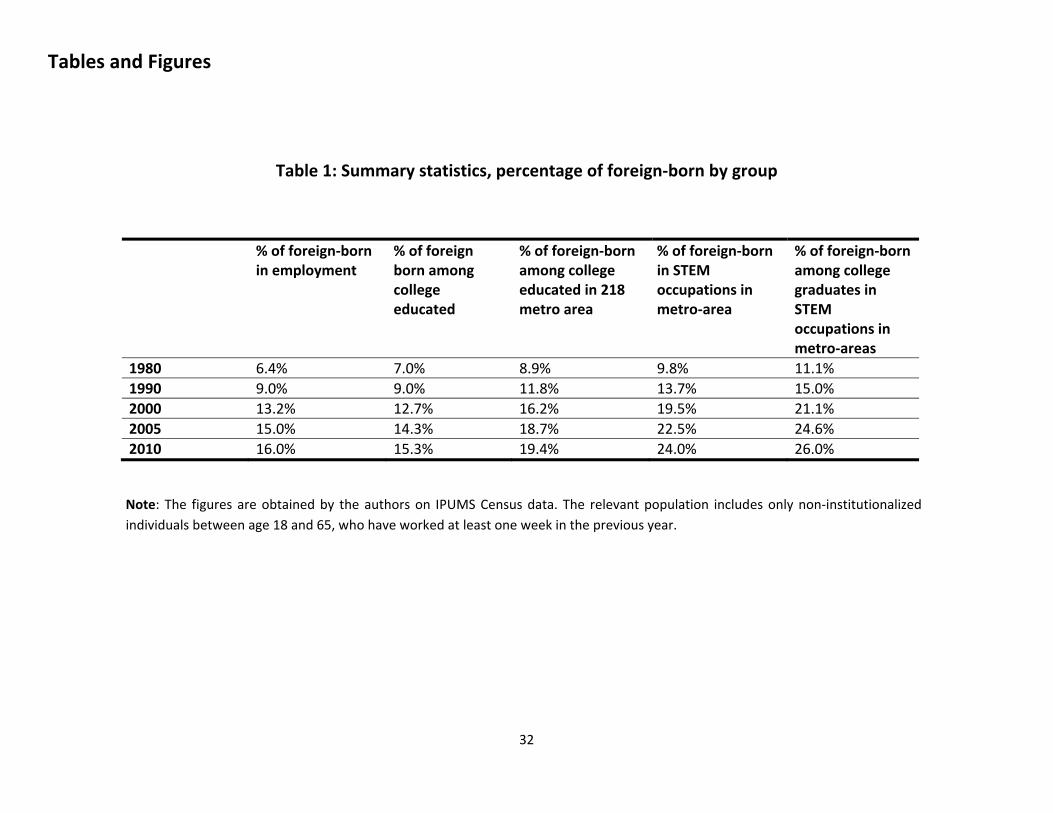
32

Tables and Figures

Table 1: Summary statistics, percentage of foreign-born by group

% of foreign-born in employment

% of foreign born among college educated

% of foreign-born among college educated in 218 metro area

% of foreign-born in STEM occupations in metro-area

% of foreign-born among college graduates in STEM occupations in metro-areas

1980 6.4% 7.0% 8.9% 9.8% 11.1% 1990 9.0% 9.0% 11.8% 13.7% 15.0% 2000 13.2% 12.7% 16.2% 19.5% 21.1% 2005 15.0% 14.3% 18.7% 22.5% 24.6% 2010 16.0% 15.3% 19.4% 24.0% 26.0%

Note: The figures are obtained by the authors on IPUMS Census data. The relevant population includes only non-institutionalized individuals between age 18 and 65, who have worked at least one week in the previous year.

33

Table 2 College Educated O*NET-STEM workers as percentage of Employment, Total 219 Metropolitan areas

Note: The figures are obtained by the authors on IPUMS Census data. The relevant population includes only non-institutionalized individuals between age 18 and 65, who have worked at least one week in the previous year.

Foreign STEM Total STEM 1980 0.3% 2.7% 1990 0.5% 3.2% 2000 0.9% 4.3% 2005 1.0% 4.3% 2010 1.1% 4.5%

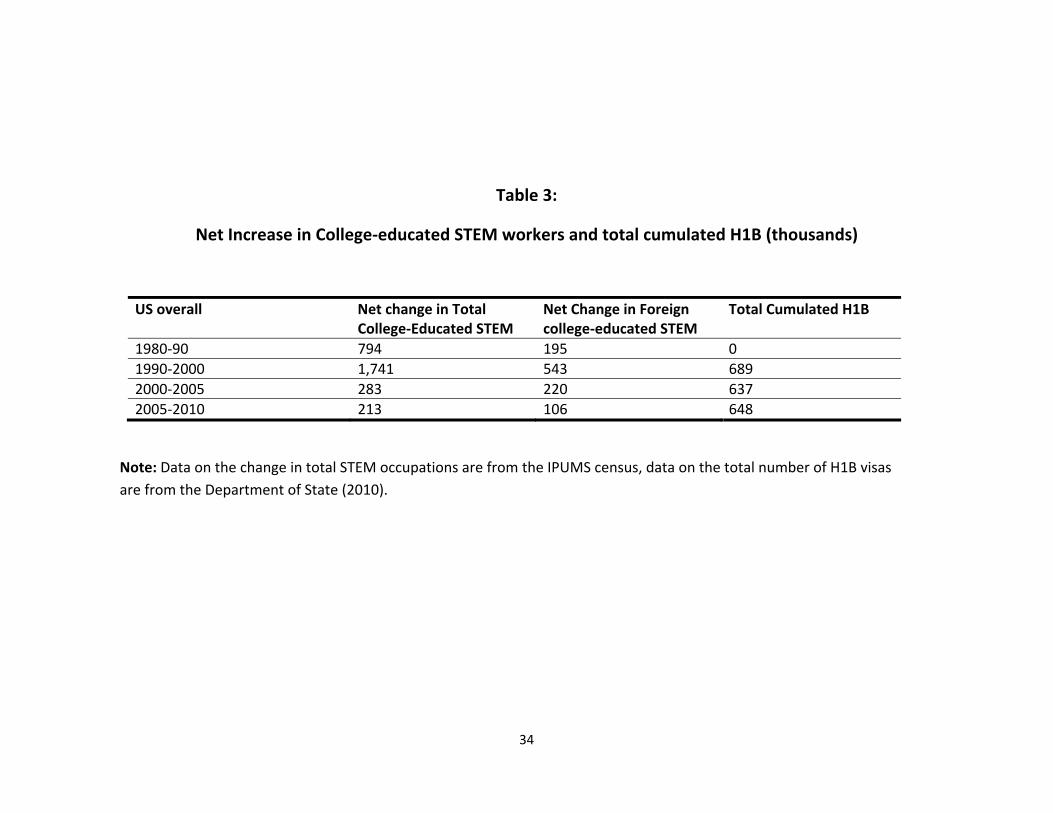
34

Table 3:

Net Increase in College-educated STEM workers and total cumulated H1B (thousands)

US overall Net change in Total College-Educated STEM

Net Change in Foreign college-educated STEM

Total Cumulated H1B

1980-90 794 195 0 1990-2000 1,741 543 689 2000-2005 283 220 637 2005-2010 213 106 648

Note: Data on the change in total STEM occupations are from the IPUMS census, data on the total number of H1B visas are from the Department of State (2010).

35

Table 4

Top 10 cities in Native- and in Foreign-STEM dependence as of 1980

Metropolitan area

Native STEM dependence, 1980

Metropolitan area Foreign STEM dependence, 1980

Richland-Kennewick-Pasco WA (Nuclear, Military)

14.7% Miami, FL 3.1%

Rockford, IL (Machine Tools, Heavy Machinery, Aerospace)

12.5%

Waterbury, CT 2.6%

Lafayette, IN (Education, Purdue)

11.5%

Los Angeles, CA 2.2%

Waterbury, CT (Clock-making, Metal Machinery)

11.4%

San Jose, CA 2.1%

Galveston-Texas City, TX (University of Texas Medical Branch)

11.3%

Hartford, CT 2.0%

Racine, WI (Johnson and Johnson, Chemicals)

11.0%

Stamford, CT 1.9%

Jackson, MI (Medical, Recording Industry)

11.02%

New Bedford, MA 1.8%

Fort Collins, CO (Colorado State University)

10.9%

Providence, RI 1.7%

Sheboygan, WI 10.9%

Bridgeport, CT 1.7%

Elkhart-Goshen, IN 10.7%

New York, NY 1.6%

Note: The ranking is among the 219 metropolitan areas that can be followed consistently from 1980 to 2010 in the UC Census.

36

Table 5

Foreign-Born, Native STEM-dependence across cities in 1980 and the H1B predicted STEM change Panel of 219 US metropolitan areas 1990-2000, 2000-2005 and 2005-2010

(1) Foreign-Born Stem dependence 1980

(2) Foreign-Born Stem dependence 1980

(3) H1B-predicted STEM growth

(4) H1B-predicted STEM growth

Foreign-STEM dependence, 1980

0.54*** (0.11)

Native STEM Dependence, 1980

-0.029 (0.032)

0.040* (0.021)

Foreign-born share of population, 1980

0.067*** (0.0065)

Observations 219 219 657 657 F-stat 0.83 103.68 4.55 20.41 Year Effects No No Yes Yes State Effects Yes Yes Yes Yes Partial R-Square ("partialling out" state and year effects)

NA NA 0.03 0.39

Note: Each column represents a separate regression. The dependent variable is written at the top of the corresponding column. Specifications (1) and (2) include 219 metropolitan areas in 1980. Regressions (3) and (4) include the H1B-predicted change in STEM in 1990-2000, 2000-2005 and 2005-2010 regressed on the 1980 of STEM dependence (foreign or native). The standard errors are heteroskedasticity robust and, when there is more than one observation per metro areas, they are clustered at the Metro-area level. The STEM definition is based on O*NET skills. ***, **,*= significant at the 1%, 5% and 10% level.

37

Table 6

Power of H1-B driven increase in Foreign STEM (O*NET definition) as predictor of Foreign STEM Panel of 219 US metropolitan areas 1990-2000, 2000-2005 and 2005-2010

Dependent Variable

(1) Change in foreign-born STEM as % of initial Employment

(2) Change in foreign-born STEM as % of initial Employment

(3) Change in foreign-born STEM as % of initial Employment

(4) As (2) pre-2005 (pre-great recession)

(5) Change in total STEM as % of initial Employment

(6) As (2) Controlling for native STEM dependence in 1980

H1-B driven growth in Foreign STEM

0.56*** (0.16)

0.67*** (0.16)

2.61** (1.18)

0.87*** (0.18)

0.77** (0.39)

0.70** (0.17)

Observations

657 657 657 438 657 657

Year Effects Yes Yes Yes Yes Yes Yes State Effects No Yes No Yes Yes Yes Metro-Area effects

No No Yes No No No

F-test of the coefficient

11.93 17.04 4.85 21.92 3.88 16.81

Note: Each column reports coefficients from a separate regression. The units of observations are 219 US Metro areas decades over two decades 1990-2000 and 2000-2010.The dependent variable is described at the top of the column. The explanatory variable is always the H1B-driven growth of Foreign-STEM jobs, as a percentage of initial employment. ***, **,*= significant at 1%, 5% and 10% level respectively.

38

Table 7

Power of H1-B driven increase in Foreign STEM as predictor of Foreign STEM: Alternative definitions and data Panel of 219 US metropolitan areas 1990-2000, 2000-2005 and 2005-2010

Dependent Variable: Change in foreign-born STEM as % of initial Employment

(1) Definition of STEM: College Educated and O*NET/STEM

(2) As (1) with metro-area fixed effects

(3) Definition of STEM: College-Major based

(4) As (3) with metro-area fixed effects

(5) As (3) with 1970 based foreign-O*NET/STEM, 116 metro areas

(6) As (1), Excluding Indians from ONET/STEM

(7) As (1), Including L1 visa in the construction of visa-entries

H1-B driven growth in Foreign STEM

0.49** (0.12)

2.20** (0.74)

0.89*** (0.13)

3.52*** (0.79)

0.32*** (0.12)

1.22** (0.40)

0.44*** (0.11)

Observations

657 657 657 657 348 657

Year Effects Yes Yes Yes Yes Yes Yes Yes State Effects Yes No Yes No No Yes Yes Metro Area effects

No Yes No Yes No No No

F-test of the coefficient

15.80 8.72 42.06 19.51 6.05 9.15 14.94

Note: Each column reports coefficients from a separate regression. The units of observations are 219 US Metro areas decades over two decades 1990-2000 and 2000-2010.The dependent variable is described at the top of the column. The explanatory variable is always the H1B-driven growth of Foreign-STEM jobs, as a percentage of initial employment.

***, **,*= significant at 1%, 5% and 10% level respectively.

39

Table 8 Direct regression of H1-B driven foreign O*NET STEM on wages/employment of native workers

219 US metropolitan areas 1990-2000, 2000-2005 and 2005-2010

Explanatory Variable: H1B-driven Growth rate of Foreign -STEM

(1) Growth rate in weekly wage, native STEM

(2) Growth rate

in weekly wage, native

College Educated

(3) Growth rate

in weekly wage, native non-College

educated

(4) Growth rate in Employment, native STEM

(5) Growth rate in Employment, native College

Educated

(6) Growth rate in employment, native non-

College educated

Basic Specification, O*NET STEM

5.33*** (1.40)

3.31*** (0.80)

-0.31 (0.66)

0.09 (0.36)

1.17 (1.02)

-2.35 (1.83)

Controlling for 1980 native STEM dependence

5.83*** (1.46)

3.40*** (0.88)

-0.11 (0.67)

0.14 (0.38)

1.35 (1.15)

-2.34 (1.90)

O*NET college educated STEM

5.26** (2.68)

2.31*** (0.74)

0.17 (0.44)

0.18 (0.15)

0.70 (0.90)

-1.58 (1.48)

College-Major STEM

-1.07 (1.24)

2.30*** (0.91)

0.02 (0.57)

0.49 (0.28)

0.14 (0.73)

-2.72 (1.91)

Pre-2005 only

8.06*** (1.93)

4.45*** (1.39)

-0.19 (0.87)

0.09 (0.50)

1.21 (1.31)

-3.61 (2.42)

Including L1 visas

3.61*** (1.11)

2.50*** (0.58)

-0.31 (0.44)

0.02 (0.24)

0.70 (0.65)

-1.60 (-1.22)

Imputation based on 1970 foreign-STEM

1.25* (0.63)

1.19** (0.58)

0.09 (0.32)

-0.14 (0.18)

-0.39 (0.49)

-1.02 (1.03)

Note: Each cell includes the estimate of the impact of H1B-driven growth of foreign-STEM on the dependent variable listed at the top of the column. The specification estimated is as (22) in the text. It includes state and year effects as controls and the industry-driven growth in the relevant employment or wage variable at the metropolitan area level (depending on the regression). ***, **, * significant at the 1, 5, 10% level.

40

Table 9 2SLS regression of foreign O*NET STEM on wages/employment of native workers

219 US metropolitan areas 1990-2000, 2000-2005 and 2005-2010

Dependent variable: Growth rate of Explanatory Variable: Growth rate of Foreign –STEM Instrument: H1B imputed growth of foreign STEM

(1) Weekly

wage, native STEM

(2) Weekly wage, native College

Educated

(3) Weekly wage,

native non-College

educated

(4) Employment, native STEM

(5) Employment, native College

Educated

(6) Employment, native non-

College educated

K-P Wald F-Statistic of

the first stage

Basic Specification, O*NET STEM

7.81** (1.93)

4.98*** (1.20)

-0.46 (0.96)

0.14 (0.52)

1.80 (1.52)

-3.51 (2.67)

17.20

Controlling for 1980 native STEM dependence

8.47** (1.87)

4.93** (1.21)

-0.17 (0.94)

0.20 (0.53)

1.94 (1.56)

-3.38 (2.75)

17.31

Pre-2005 only

9.26** (2.19)

5.29*** (1.53)

-0.17 (0.97)

0.11 (0.58)

1.38 (1.42)

-4.02 (2.70)

22.3

Including L1 visas

8.09*** (2.24)

5.80*** (1.59)

-0.71 (1.03)

0.61 (0.53)

1.64 (1.49)

-3.67 (2.67)

15.09

IV constructed without Indian Immigrants

6.88*** (2.01)

4.72*** (1.26)

-0.36 (0.90)

-0.30 (0.65)

0.29 (1.70)

-4.24 (2.77)

16.41

Imputation of IV-based on 1970 foreign-STEM

6.37*** (2.51)

6.08*** (1.98)

0.44 (1.40)

-1.18 (2.09)

-3.26 (5.93)

-6.86 (9.42)

3.17

1970-based IV, pre 2005 only

6.58** (3.02)

5.30*** (1.82)

0.68 (1.50)

-1.14 (1.50)

-2.67 (3.64)

-3.22 (7.83)

4.52

Total STEM as explanatory

7.12*** (2.90)

4.30*** (1.91)

-0.36 (0.92)

N.A. 1.58* (0.82)

-3.03 (3.59)

3.88

OLS, Basic Specification

4.61*** (1.21)

2.83*** (0.70)

1.59*** (0.43)

1.25*** (0.26)

3.73*** (1.35)

4.57*** (1.48)

N.A.

Note: Each cell includes the 2SLS estimate of the impact of growth of foreign-STEM on the dependent variable listed at the top of the column. The instrument used is the H1-B driven growth of foreign- STEM workers. The specification estimated is as (23) in the text. It always includes state and year effects as controls and the industry-driven growth in the relevant employment or wage (depending on the regression). The last row shows the OLS estimate of the Basic Specification. The standard errors are heteroskedasticity-robust and clustered at the metro-area level. ***, **, * significant at the 1, 5, 10% level.

41

Table 10 2SLS regression of foreign STEM on wages/employment of native workers: Extension and robustness

219 US metropolitan areas 1990-2000, 2000-2005 and 2005-2010

Dependent variable: Growth rate of Explanatory Variable: Growth rate of Foreign –STEM Instrument: H1B imputed growth of foreign STEM

(1) Weekly

wage, native STEM

(2) Weekly wage, native College

Educated

(3) Weekly wage,

native non-College

educated

(4) Employment, native STEM

(5) Employment, native College

Educated

(6) Employment, native non-

College educated

K-P Wald F-Statistic of

the first stage

O*NET STEM, College educated

11.05* (5.92)

4.84*** (1.53)

0.35 (0.84)

0.18 (0.15)

0.70 (0.92)

-1.58 (1.43)

15.32

Major-Based STEM

2.10 (1.64)

2.64*** (0.88)

0.03 (0.61)

0.62 (0.38)

0.17 (1.89)

-3.23 (2.17)

42.70

Major-Based STEM, with Metro-area fixed effects

1.98 (2.40)

6.88*** (1.92)

1.47 (1.42)

0.60 (0.47)

-0.31 (1.79)

-6.78 (3.54)

21.67

O*NET STEM, College educated Pre-2005 only

11.90* (6.30)

5.80*** (2.12)

0.70 (1.01)

0.61 (0.49)

1.54 (2.39)

-4.23 (3.23)

14.95

Total STEM (O*NET, College educated) as explanatory

6.56** (3.27)

2.87*** (0.79)

0.20 (0.47)

N.A. 1.70 (0.90)

-1.71 (2.01)

19.55

OLS, Major-Based STEM Specification

0.62 (1.01)

3.21*** (0.62)

1.52*** (0.40)

1.20*** (0.26)

4.25*** (1.59)

2.90** (1.40)

N.A.

Note: Each cell includes the 2SLS estimate of the impact of growth of foreign-STEM on the dependent variable listed at the top of the column. The instrument used is the H1-B driven growth of foreign- STEM workers. The specification estimated is as (23) in the text. It always includes state and year effects as controls and the industry-driven growth in the relevant employment or wage (depending on the regression). The last row shows the OLS estimate of the Basic Specification not including the industry-driven growth. The standard errors are heteroskedasticity-robust and clustered at the metro-area level. ***, **, * significant at the 1, 5, 10% level.

42

Table 11 2SLS regression of foreign STEM on House rental prices

219 US metropolitan areas 1990-2000, 2000-2005 and 2005-2010

Explanatory Variable: Growth rate of Foreign –STEM Instrument: H1B imputed growth of foreign STEM

(1) Average

Rent, College

educated

(2) Median Rent,

College educated

(3) Average Rent, Non-College

educated

(4) Median Rent, Non-College

educated

K-P Wald F-Statistic of

the first stage

Basic Specification, O*NET STEM

2.34 (1.47)

4.11*** (1.29)

-1.76 (1.38)

-1.90 (1.45)

16.46

Pre-2005 only

4.98*** (1.69)

5.16** (1.63)

-1.19 (1.37)

-1.33 (1.30)

22.01

Pre-2005 Including L1 visas

4.97*** (1.67)

5.30*** (1.86)

-1.37 (1.40)

-1.14 (1.50)

19.86

Pre 2005, O*NET, college educated STEM

4.76*** (2.02)

5.89*** (2.13)

-0.33 (1.47)

-0.77 (1.44)

14.99

Basic Specification, OLS 3.56*** (1.03)

3.11*** (0.96)

1.77** (0.68)

0.91 (0.68)

N.A.

.

Note: Each cell includes the 2SLS estimate of the impact of growth of foreign-STEM on the dependent variable listed at the top of the column. The instrument used is the H1-B driven growth of foreign- STEM workers. The specification estimated is as (23) in the text. It always includes state and year effects as controls and the industry-driven growth in the relevant employment or wage (depending on the regression). The last row shows the OLS estimate of the Basic Specification not including the industry-driven growth. The standard errors are heteroskedasticity-robust and clustered at the metro-area level. ***, **, * significant at the 1, 5, 10% level.

43

Table 12 2SLS regression of foreign STEM on wages/employment of native workers: Split of non-college in2 groups

219 US metropolitan areas 1990-2000, 2000-2005 and 2005-2010

Dependent Variable: Growth rate of Explanatory Variable: Growth rate of Foreign –STEM Instrument: H1B imputed growth of foreign STEM

(1) Weekly

wage, native HS

graduates

(2) Weekly wage, HS dropouts

(3) Employment,

native HS graduates

(4) Employment,

native HS dropouts

K-P Wald F-Statistic of

the first stage

Basic Specification, O*NET STEM

-0.50 (1.08)

-4.29 (2.70)

-4.03 (2.80)

0.11 (0.48)

13.44

Controlling for 1980 native STEM dependence

-0.17 (1.06)

-4.30 (2.65)

-3.89 (2.83)

0.23 (0.47)

13.34

Pre-2005 only

0.07 (1.04)

-2.26 (2.75)

-4.38* (2.37)

0.22 (0.41)

24.19

Including L1 visas

-0.90 (1.12)

-3.66 (2.60)

-4.06 (2.99)

0.16 (0.5)

11.80

All STEM as explanatory variable

-0.49 (1.21)

-3.06 (2.48)

-4.26 (4.61)

0.28 (0.35)

3.67

Basic Specification, OLS 0.56** (0.13)

0.64* (0.31)

3.23** (0.34)

0.59** (0.10)

N.A.

Note: Each cell includes the 2SLS estimate of the impact of growth of foreign-STEM on the dependent variable listed at the top of the column. The instrument used is the H1-B driven growth of foreign- STEM workers. The specification estimated is as (23) in the text. It always includes state and year effects as controls and the industry-driven growth in the relevant employment or wage (depending on the regression). The last row shows the OLS estimate of the Basic Specification not including the industry-driven growth. The standard errors are heteroskedasticity-robust and clustered at the metro-area level. ***, **, * significant at the 1, 5, 10% level.

44

Table 13: Effects of foreign STEM on employment by Industry

219 US metropolitan areas 1990-2000, 2000-2005 and 2005-2010 Explanatory Variable: Growth rate of Foreign –STEM Instrument: H1B imputed growth of foreign STEM

(1) Dep. Variable:

total Employment 2SLS

(2) Dep. Variable: total

Employment Direct regression

(3) Dep. Variable:

College –Educated Employment

2SLS

(4) Dep. Variable:

College –Educated Employment

Direct Regression Low Human Capital Private Sectors

Construction

-0.23 (0.35)

-0.11 (0.18)

0.04 (0.05)

0.02 (0.02)

Transportation

-0.18 (0.24)

-0.09 (0.12)

0.09 (0.06)

0.04 (0.03)

Wholesale

-0.19 (0.16)

-0.09 (0.08)

-0.06 (0.05)

-0.03 (0.03)

Manufacturing

0.55 (1.16)

0.27 (0.55)

0.20 (0.32)

0.098 (0.15)

Retail

0.05 (0.72)

0.02 (0.37)

0.24 (0.15)

0.12* (0.07)

High Human Capital Private Sectors Finance

0.63 (0.62)

0.31 (0.31)

0.63 (0.47)

0.31 (0.24)

Business

0.44 (0.30)

0.22 (0.15)

0.67*** (0.20)

0.33*** (0.08)

Professional Services

0.26 (1.16)

0.13 (0.59)

1.30** (0.79)

0.64* (0.35)

Non-Private Sector Public Sector

-0.19 (0.29)

-0.09 (0.15)

0.06 (0.10)

0.03 (0.05)

Note: Each cell includes the 2SLS estimate of the impact of growth of foreign-STEM on the dependent variable listed at the top of the column, within the sector listed in the row. The instrument used is the H1-B driven growth of foreign- STEM workers. The standard errors are heteroskedasticity-robust and clustered at the metro-area level. ***, **, * significant at the 1, 5, 10% level.

45

Table 14

Foreign STEM and “Innovative” skills of College-Educated Natives

Dependent Variable (1) Growth in “Creative” O*NET

skills of native college educated

(2) Growth in “Problem solving” O*NET skills of native college

educated Direct Regression

H1B-driven Growth rate of College educated Foreign

O*NET STEM

1.33*** (0.36)

0.83** (0.36)

2SLS regression Growth rate College-educated

O*NET STEM 1.30*** (0.46)

0.81** (0.39)

First Stage F-stat of instrument 19.71 19.71

Note: each cell shows the coefficient from a separate regression. The dependent variable is the O*NET intensity index of “creative skills”, “Problem-Solving” skills and STEM Skills calculated based on occupation of the native college-educated workers in the Metropolitan area. Observations are 219 metropolitan areas in 1990, 2000, 2005 and 2010. The standard errors are heteroskedasticity robust and clustered by Metro area. ***, **, *= significant at the 1%, 5% and 10% level respectively.

46

Table 15 Implied Macro effect of foreign STEM growth on TFP growth and on skill-biased productivity

(1) Average

yearly Growth in Foreign-

STEM (as % of

employment)

(2) φA

Elasticity of A to STEM

(3)φB

Elasticity of β to STEM

(4) Implied effect on average yearly TFP

growth

(5) Implied

Change in average

yearly Skill-biased

Productivity: β/(1-β)

(6) Actual

US TFP average yearly

growth, from

Fernald (2010)

(7) Change in

average yearly skill-

biased productivity implied by the US data

(4)/(6) (5)/(7)

Average value of bw,NS from Table 9. Insignificant=0

1990-2000 0.06% 2.75 3.57 0.38% 0.23% 1.01% 1.7% 0.38 0.14 2000-2010 0.02% 2.75 3.57 0.10% 0.06% 0.77% 1.8% 0.12 0.03 Average 0.04% 2.75 3.57 0.24% 0.14% 0.89% 1.75% 0.27 0.08

Average value of bw,NS from Table 9. Average point estimate of bL,E

1990-2000 0.06% 2.92 4.94 0.41% 0.32% 1.01% 1.7% 0.41 0.19 2000-2010 0.02% 2.92 4.94 0.10% 0.08% 0.77% 1.8% 0.13 0.04 Average 0.04% 2.92 4.94 0.26% 0.20% 0.89% 1.75% 0.29 0.11

Note: The table uses the formulas in the appendix to calculate the implied elasticity φA and φ.B. We then use the growth of STEM workers as % of the employment to calculate the implied effects on TFP and skill-biased productivity. The figures on actual TFP growth were taken from Fernald (2010) and the figures for the data-implied change in skill-bias were calculated using the census 1980, 1990, 2000 and 2010 data on employment and wages of college and non-college educated and the formula implied by our model in footnote 15 of the text.

47

Table 16 Implied Min-Max Inter-city differences in TFP growth

(1) Min-Max intercity

difference in foreign STEM

growth (as % of employment)

(2)φA

Elasticity of A to STEM

(3) Implied

Min-Max difference

in TFP growth

(4) Actual Min-

Max Difference

TFP growth, from Average

Wages

(3)/(4)

Average value of bw,NS from Table 9. Insignificant=0

1990-2000 0.70% 2.75 4.48% 4.40% 1.02 2000-2010 0.26% 2.75 1.67 3.30% 0.50 Average 0.48% 2.75 3.08% 3.85% 0.76

Average value of bw,NS from Table 9. Average point estimate of bL,E

1990-2000 0.70% 2.92 4.76% 4.40% 1.08 2000-2010 0.26% 2.92 1.77% 3.30% 0.54 Average 0.48% 2.92 3.27% 3.85% 0.80

Note: The table uses the formulas in the appendix to calculate the implied elasticity φA and φ.B. We then use the growth of foreign STEM workers as % of the employment to calculate the implied effects on TFP. The actual TFP min-max difference is obtained as the difference in growth of average wages in cities. City with lowest growth of foreign STEM: in 1990’s Terre Haute, IN, in 2000’s Wichita Falls, TX. With highest foreign STEM growth: 1990’s San Jose, CA 2000’s Seattle-Everett, WA.

48

Figure 1

Note: The data on H1B visas and their cap are from the Department of State

49

Figure 2

Note: The rates of Foreign and Native STEM dependence are calculated using 1980 Census data for 219 Metro Areas.

0.0

1.0

2.0

3Fo

reig

n S

TEM

/Pop

.04 .06 .08 .1 .12 .14Native STEM/Pop

US Metro areas, 1980 Native and Foreign STEM dependence

Coefficient=-0.044Standard error=0.028

50

Figure 3

Note: The figures are calculated using 1980 Census data. The population of reference to calculate the share of foreign born in a city is the total adult (18-65) population not institutionalized.

0.0

1.0

2.0

3Fo

reig

n ST

EM

/Pop

0 .1 .2 .3 .4Foreign Born/Pop

US Metro areas, 1980Foreign-STEM dependence and share of Foreign-Born

Coefficient=-0.071Standard error=0.006

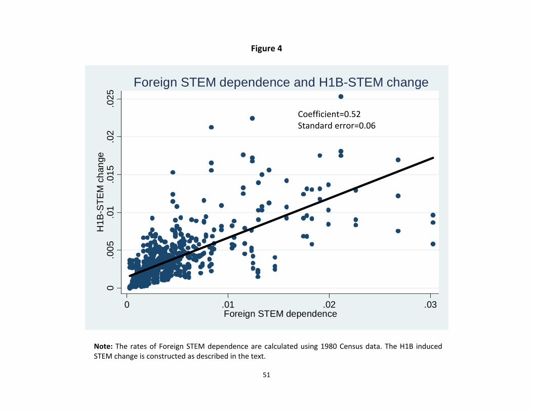
51

Figure 4

Note: The rates of Foreign STEM dependence are calculated using 1980 Census data. The H1B induced STEM change is constructed as described in the text.

0.0

05.0

1.0

15.0

2.0

25H

1B-S

TEM

cha

nge

0 .01 .02 .03Foreign STEM dependence

Foreign STEM dependence and H1B-STEM change

Coefficient=0.52Standard error=0.06

52

Figure 5

Note: The rates of native STEM dependence are calculated using 1980 Census data. The H1B induced STEM change is constructed as described in the text.

0.0

05.0

1.0

15.0

2.0

25H

1B-S

TEM

cha

nge

.04 .06 .08 .1 .12 .14Native STEM dependence

Native STEM dependence and H1B-STEM change

Coefficient=0.028Standard error=0.014

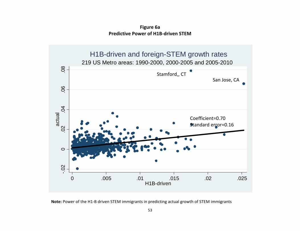
53

Figure 6a Predictive Power of H1B-driven STEM

Note: Power of the H1-B driven STEM immigrants in predicting actual growth of STEM immigrants

-.02

0.0

2.0

4.0

6.0

8ac

tual

0 .005 .01 .015 .02 .025H1B-driven

219 US Metro areas: 1990-2000, 2000-2005 and 2005-2010H1B-driven and foreign-STEM growth rates

San Jose, CAStamford,, CT

Coefficient=0.70Standard error=0.16

54

Figure 6b

Predictive Power of H1B-driven STEM, without outliers

Note: As figure 6a without Stamford, CT and San Jose CA

-.02

0.0

2.0

4ac

tual

0 .005 .01 .015 .02 .025H1B-driven

omitting Stamford, CT and San Jose, CAH1B-driven and foreign STEM growth rates

Coefficient=0.44Standard error=0.07

55

Appendix Table A1, Part A Occupations classified as O*NET- STEM, skills at the top 10% of the distribution in 2000 Chemical engineers Veterinarians

Civil engineers Programmers of numerically controlled machine tool

Not-elsewhere-classified engineers Cementing and gluing machine operators Physicists and astronomers Geologists Chemists Chemical technicians Sales engineers Supervisors of agricultural occupations Management analysts Heating, air conditioning, and refrigeration mechanic Petroleum, mining, and geological engineers Carpenters Licensed practical nurses Boilermakers Electrical engineer Plant and system operators, stationary engineers Industrial engineers Chief executives and public administrators Operations and systems researchers and analysts Biological technicians Actuaries Statistical clerks Mathematicians and mathematical scientists Farm managers, except for horticultural farms Atmospheric and space scientists Supervisors of mechanics and repairers Medical scientists Machinery maintenance occupations Surveyors, cartographers, mapping scientists and t Water and sewage treatment plant operators Other science technicians Lathe, milling, and turning machine operatives Elevator installers and repairers Drilling and boring machine operators Plasterers Construction inspectors Rollers, roll hands, and finishers of metal Biological scientists Agricultural and food scientists Airplane pilots and navigators Engineering technicians, n.e.c. Millwrights Drafters Drillers of oil wells Plumbers, pipe fitters, and steamfitters Explosives workers Aerospace engineer Tool and die makers and die setters Mechanical engineers Machinists Computer software developers Power plant operators Managers of medicine and health occupations Machine operators, n.e.c. Automobile mechanics Secondary school teachers

56

Table A1, Part B Occupations classified as College-Major-STEM, those with more than 25% of workers with a STEM college degree Pharmacists Metallurgical and materials engineers, variously p Chemists Occupational therapists Optometrists Other health and therapy Chemical engineers Atmospheric and space scientists Physicists and astronomers Computer software developers Medical scientists Industrial engineers Podiatrists Agricultural and food scientists Dentists Physical therapists Physicians Sales engineers Civil engineers Mathematicians and mathematical scientists Geologists Physicians' assistants Biological scientists Therapists, n.e.c. Aerospace engineer Airplane pilots and navigators Veterinarians Clinical laboratory technologies and technicians Speech therapists Dietitians and nutritionists Not-elsewhere-classified engineers Subject instructors (HS/college) Petroleum, mining, and geological engineers Computer systems analysts and computer scientists Electrical engineer Vocational and educational counselors Mechanical engineers Management analysts Psychologists Chemical technicians Actuaries Biological technicians

57

Table A1, PartC List of college major classified as STEM

Animal Sciences Family and Consumer Sciences Food Science Library Science Metallurgical Engineering Plant Science and Agronomy Biology Mining and Mineral Engineering Soil Science Biochemical Sciences Naval Architecture and Marine Engineer Environmental Science Botany Nuclear Engineering Computer and Information Systems Molecular Biology Petroleum Engineering Computer Programming and Data Processing Ecology Miscellaneous Engineering Computer Science Genetics Engineering Technologies Information Sciences Microbiology Engineering and Industrial Management Computer Information Management and Sec Pharmacology Electrical Engineering Technology Computer Networking and Telecommunication Physiology Industrial Production Technologies General Engineering Zoology Mechanical Engineering Related Technology Aerospace Engineering Neuroscience Miscellaneous Engineering Technologies Biological Engineering Miscellaneous Biology Medical Technologies Technicians Architectural Engineering Mathematics Health and Medical Preparatory Programs Biomedical Engineering Applied Mathematics Pharmacy, Pharmaceutical Sciences, and Chemical Engineering Statistics and Decision Science Treatment Therapy Professions Civil Engineering Military Technologies Geosciences Computer Engineering Nutrition Sciences Oceanography Electrical Engineering Mathematics and Computer Science Physics Engineering Mechanics, Physics, and Sci Cognitive Science and Biopsychology Materials Science Environmental Engineering Physical Sciences Multi-disciplinary or General Science Geological and Geophysical Engineering Astronomy and Astrophysics Nuclear, Industrial Radiology, and Bio Industrial and Manufacturing Engineering Atmospheric Sciences and Meteorology Psychology Materials Engineering and Materials Sci Chemistry Educational Psychology Mechanical Engineering Geology and Earth Science Clinical Psychology General Medical and Health Services Miscellaneous Psychology Counseling Psychology Communication Disorders Sciences and Se Transportation Sciences and Technologies Industrial and Organizational Psychology Social Psychology

58

Table A2: H1-B visas composition by nationality

nationality percentage of

total, 1990-2000 percentage of

total, 2000-2010 Africa 3% 2% Canada 0% 0% China 5% 7% Eastern Europe 5% 4% India 45% 47% Japan 3% 3% Korea 1% 3% Mexico 3% 4% Oceania 2% 1% Philippines 3% 3% Rest of Americas 5% 8% Rest of Asia 10% 9% Western Europe 16% 11% Other 0% 0% Total H1B visas 709505 1321028