stephen p. holland and michael moore · including opportunities to borrow or bank permits through...
TRANSCRIPT

NBER WORKING PAPER SERIES
WHEN TO POLLUTE, WHEN TO ABATE? INTERTEMPORAL PERMIT USE INTHE LOS ANGELES NOX MARKET
Stephen P. HollandMichael Moore
Working Paper 14254http://www.nber.org/papers/w14254
NATIONAL BUREAU OF ECONOMIC RESEARCH1050 Massachusetts Avenue
Cambridge, MA 02138August 2008
The authors thank Frank Wolak and seminar participants at UC-Santa Barbara and the UC EnergyInstitute for comments. Thanks also to Ann Ferris and Peter Landry for research assistance, and toDanny Luong for sharing his expertise on the RECLAIM program. This research was supported inpart by a grant from the U.S. Environmental Protection Agency’s STAR program. Holland also thanksthe University of California Energy Institute for research support during this project. The views expressedherein are those of the author(s) and do not necessarily reflect the views of the National Bureau ofEconomic Research.
NBER working papers are circulated for discussion and comment purposes. They have not been peer-reviewed or been subject to the review by the NBER Board of Directors that accompanies officialNBER publications.
© 2008 by Stephen P. Holland and Michael Moore. All rights reserved. Short sections of text, notto exceed two paragraphs, may be quoted without explicit permission provided that full credit, including© notice, is given to the source.
When to Pollute, When to Abate? Intertemporal Permit Use in the Los Angeles NOx MarketStephen P. Holland and Michael MooreNBER Working Paper No. 14254August 2008JEL No. L5,Q5
ABSTRACT
Intertemporal tradability allows an emissions market to reduce abatement costs. We study intertemporaltrading of nitrogen oxides permits in the RECLAIM program in Southern California. A theoreticalmodel captures the program's key intertemporal features: two overlapping permit cycles, two compliancecycles for facilities, and tradable permits. We characterize the competitive equilibrium; show thatit is cost effective; and demonstrate the firms' incentive to delay abatement, i.e., to trade intertemporally.Using model extensions to explore market design issues, an arbitrage condition implies that the equilibriumis invariant to overlapping compliance cycles, but depends crucially on overlapping permit cycles.We empirically investigate intertemporal trading of permits using panel data on RECLAIM facilitiesfor 1994-2006. Facilities undertake trading by using a considerable proportion of permits of the oppositecycle. We econometrically test two theoretical propositions -- delayed abatement and trading acrosscycles -- with a difference-in-differences estimator. The results neither contradict nor provide conclusivesupport of the theory.
Stephen P. HollandBryan School of Business and EconomicsUniversity of North Carolina, GreensboroP.O. Box 26165Greensboro, NC 27402-6165and [email protected]
Michael MooreSchool of Natural Resources & EnvironmentUniversity of MichiganAnn Arbor, MI [email protected]

1. Introduction
Markets for pollution emissions are now the presumptive approach to implementing
environmental regulation. This is due, primarily, to the widely hailed success of the U.S. sulfur dioxide
(SO2) market under the Clean Air Act’s Acid Rain Program (Ellerman et al. 2000; Joskow, Schmalensee,
and Bailey 1998). Building on this, a nitrogen oxides (NOx) market was introduced in 19 eastern states in
2003, and a European Union carbon dioxide (CO2) market began as the centerpiece of compliance with
the Kyoto Protocol climate treaty in 2005. Markets are also part of regional initiatives within the United
States to limit greenhouse gas emissions. Emissions markets – or cap-and-trade programs – are the
“grand” policy experiments of environmental regulation (Stavins 1998; Kruger and Pizer 2004).
A key component of any emissions market is the temporal dimension of trading and use,
including opportunities to borrow or bank permits through time (Tietenberg 2006). Flexible
intertemporal trading allows firms to minimize pollution abatement costs over time. However, the
additional flexibility from intertemporal trading can lead to hotspots – short periods with high emissions –
which may lead to high damage costs for some pollutants.
We study intertemporal trading in one of the longest running emissions markets, the Regional
Clean Air Incentives Market (RECLAIM). Begun in 1994, RECLAIM established tradable permits for
NOx and SO2 emissions as part of a program to reduce smog in the Los Angeles air basin. A unique
feature of RECLAIM – that permits and polluting facilities are assigned to one of two overlapping cycles,
with trading allowed across cycles – creates opportunities for intertemporal trade. Early summaries of the
program noted that the overlapping cycles were designed to avoid insufficient liquidity in the market at
the end of a compliance cycle (e.g., Carlson and Sholtz 1994). More recently, Ellerman, Joskow, and
Harrison (2003) observed that the overlapping cycles allow “limited temporal flexibility.”1 However,
overlapping cycles and intertemporal trading have not been analyzed formally or comprehensively for the
1 In contrast, Schwarze and Zapfel (2000) claim that “RECLAIM does not provide for any kind of inter-temporal trading” when comparing RECLAIM to the SO2 allowance market.
2
RECLAIM program.2
We investigate the theoretical and empirical implications of RECLAIM’s overlapping cycles with
three research questions. What are the equilibrium properties of the intertemporal market for RECLAIM
permits? Can the program achieve cost-effective abatement? Are the empirical results consistent with
predictions derived from the theoretical market equilibrium?
In the theoretical model of the intertemporal RECLAIM market, regulated firms are assigned to
one of two compliance cycles. The firms minimize discounted pollution abatement costs and permit costs
while meeting annual compliance requirements with valid permits of either cycle. We characterize the
market’s competitive equilibrium and derive results on cost effectiveness, invariance of the equilibrium to
parameter changes, delayed abatement, and the intertemporal pattern of prices. 3 The model clarifies the
opportunities for intertemporal arbitrage that arise from the two overlapping cycles.
We extend the model to explore various market design options which arise with overlapping
cycles. First, we ask whether trading is cost effective when firms cannot trade across permit cycles. We
then analyze the equilibrium when permit cycles are overlapping, but firms’ compliance cycles are not,
and vice versa. Finally, we analyze multiple overlapping cycles.
Using data on permits and emissions from all RECLAIM facilities from 1994 through mid 2006,
we evaluate several theoretical predictions of the model. First, using aggregate data, we ask whether
firms used all of the permits of each vintage, as predicted by the model, focusing on the years in which
the program was clearly binding. We then verify that firms do indeed trade across cycles. Second, using
data on facility emissions, we use difference-in-differences estimators to test two predictions: whether
facilities delay abatement and whether there are no differences in emissions across compliance cycles.
The paper proceeds in Section 2 by discussing the relevant background of the RECLAIM
2 Unrestricted banking was ruled out under RECLAIM “because of concerns that the ability to use banked emissions might lead to substantial increases in actual emissions in some future year, and thus delay compliance with ambient air quality standards” (Ellerman, Joskow, and Harrison 2003, 21). 3 Kling and Rubin (1997) demonstrated that bankable and borrowable permits are cost effective but not dynamically efficient. We find a similar result. Like Schennach (2000), our competitive equilibrium has characteristics similar to the equilibrium in an exhaustible resource market.

3
program. Section 3 analyzes the model of the RECLAIM market, and Section 4 uses the model to explore
various market design issues. Section 5 describes the data. Section 6 presents the empirical results,
which include descriptive analysis of aggregate permit data and econometric analysis of facility emissions
data. Section 7 concludes.
2. The RECLAIM Program 2.1 Basic Features
The RECLAIM program established a cap-and-trade program for NOx and SO2 in the Los
Angeles air basin beginning January 1, 1994. The region has consistently suffered some of the worst
smog in the United States (SCAQMD 1994). RECLAIM’s original goal was to comply, by 2003, with
the National Ambient Air Quality Standards (NAAQS) for ground-level ozone and particulates. The
program thus defined steadily decreasing caps for NOx and SO2 emissions.4 The South Coast Air Quality
Management District (SCAQMD) administers the program.5
The program defines a RECLAIM Trading Credit (RTC) as the tradable emissions permit. One
RTC entitles the owner to emit one pound of pollution within a twelve-month interval. Two types of
RTC’s exist – NOx and SO2 – and thus two distinct markets operate in the program. The SO2 market is
relatively thin (Gangadharan 2000), so our analysis focuses on the NOx market. The regulated entity
under RECLAIM is a pollution-emitting facility. Initial allocations of RTC’s were distributed free of
charge to facilities. Over 300 facilities have used NOx RTC’s in each year of the program. A single firm
operates more than one facility in some cases.
A key feature of RECLAIM is its two overlapping cycles. Roughly equal numbers of facilities
are assigned to each of the two compliance cycles. Facilities in compliance cycle 1 complete their twelve-
month cycle at the end of the calendar year (December 31), while facilities in compliance cycle 2
complete their twelve-month cycle at the end of the fiscal year (June 30). RTC’s allocated to cycle 1 4 Even with the 75% reduction in the NOx cap by 2007, the region continues to exceed the NAAQS ozone standard (USEPA 2007). Program amendments in 2005 therefore require an additional 2,800 tons of reductions (about 25% below the 2007 cap) between 2007 and 2011. 5 The regulatory rules for the RECLAIM program are available at the SCAQMD website (SCAQMD 2007b). These rules are the source for much of the program information reported here.
4
facilities are valid from January 1 through December 31. RTC’s allocated to cycle 2 facilities, in contrast,
are valid from July 1 through June 30. Every facility then can comply using valid permits of either
cycle.6 For example, cycle 1 firms can purchase and use cycle 2 RTC’s for compliance, although the
RTC’s remain subject to the cycle 2 time limit. Cycle 2 firms can do likewise. We refer to the staggered
cycles as the overlapping compliance cycles and overlapping permit cycles features of the program.7
A cycle thus serves as a characteristic of both a facility and an RTC. Although these two
characteristics are separable in principle, they are linked in RECLAIM.8 For example, each cycle 1
facility is allocated only cycle 1 permits and, as well, must demonstrate compliance on a calendar year
basis in each year.
The RECLAIM program includes a monitoring requirement,9 a reporting protocol, and a penalty
structure for excess emissions. All facilities report emissions as part of a process known as Quarterly
Certification of Emissions. The penalty structure for excess emissions (“exceedances”) is defined as an
RTC quantity, a discretionary monetary fine, and discretionary limitations on the facility’s ability to
operate. A facility’s allocation is reduced 1:1 by the amount of the excess in the year subsequent to the
determination; this is referred to as an “exeedance deduction.” A fine can also accompany the deduction,
although SCAQMD can negotiate the amount of fine, subject to limitations within the RECLAIM
regulations and California state laws. In practice, fines are levied in most cases with the amounts varying
according to the specific causes of the exceedances. The penalty structure also provides for the authority
to impose additional permit conditions that specify requirements to prevent future exceedances.
6 To comply successfully, the number of valid RTC’s that a facility owns must equal or exceed its annual emissions. 7 The program also defines two spatial zones, coastal and inland. Due to the natural drift of smog from west to east, spatial trading from the inland zone to the coastal zone could exacerbate pollution. RTC’s allocated to facilities in the coastal zone thus can be traded to cover emissions in the inland zone, but not vice versa. Gangadharan (2004) shows that, as expected, the price of a coastal-zone RTC is higher on average than the price of an inland-zone RTC. 8 Carlson and Sholtz (1994) recognize this separability by noting that facilities could have received a “mixed allocation” of permits of each cycle. 9 A regulated NOx facility is classified as a major source, a large source, or a NOx process unit. A major source must use a continuous emissions monitoring system (or another system with equivalent accuracy). A large source has the option, instead, to install a continuous process monitoring system. A process unit can be monitored manually by a fuel meter or other device.

5
2.2 Performance10
One perspective on the RECLAIM program comes from examining, at an aggregate level, permit
allocations and usage over time.11 Figure 1 shows the total number of permits of each vintage based on
their dates of expiration. The temporal declines in the initial allocations and available permits reflect the
RECLAIM program’s goal of reducing emissions. The figure also shows the number of permits of each
cycle used by facilities to cover their emissions.
In the figure, the initial allocations are the RTC’s initially given to the facilities, and available
RTC’s are all permits available for the facilities to cover emissions. These can differ for several reasons.
First, credits may be unavailable due to exceedance deductions. For example, 2.7 million permits
expiring in December 1997 were deducted for prior exceedances. Second, permits can be created for a
variety of mobile source credits. Through 2005, approximately 250,000 RTC’s were created through
mobile source credits. Finally, permits were created and subsequently subtracted under an executive
order and a mitigation fund in response to the California electricity crisis of 2000-2001.
The RECLAIM market can be divided into three periods: 1994-1999, 2000-2001, and 2002-2006.
The first period’s defining characteristic is a non-binding cap at the aggregate level (Figure 1). The non-
binding cap was set intentionally to test whether the program, indeed, could be implemented successfully
(Tietenberg 2006). However, the excess supply meant that the decline in available permits did not lead to
an equivalent reduction in emissions. Not surprisingly, average prices for current NOx permits were very
low during this period: $154 per ton in 1996; $227 per ton in 1997; and $451 per ton in 1998.
Although prices were low, market activity appeared robust in the program’s early years. Klier et
al. (1997) found that roughly half the facilities participated in the RTC markets during 1995.
Gangadharan (2000) assessed the factors that affected a facility’s decision to trade or not in 1995 and
1996 and argued that trading begets trading, i.e., the probability that a facility trades increases if the
10 Comprehensive evaluations of RECLAIM are available. The Annual RECLAIM Audit Reports, published by SCAQMD, thoroughly describe many aspects of the program; these reports are available at the district’s website. USEPA (2002, 2006) and Harrison (2004) also provide descriptions and evaluations of the program. 11 Facility-level data on RTC holdings, compliance, transactions, and emissions came from a public records request to the SCAQMD.
6
facility traded previously. Gangadharan (2004) also assessed the factors that affected RTC prices.
Institutional features, type of seller (broker or facility), and year of transaction explain price levels.
RECLAIM’s second period reflects crisis contagion: the perceived crisis in RECLAIM as a result
of the California electricity crisis of 2000-2001. The number of permits used closely tracked the number
of permits available during this period (Figure 1). The electricity crisis was characterized, in part, by
enormous price spikes in the wholesale electricity market (Joskow 2001). Faced with high prices amidst
summertime electricity demand, electricity generators in the Los Angeles region ramped up their output.
Electricity generation at natural-gas-fueled plants is a major source of NOx emissions; generators thus
were in a buying position on the NOx market.12 RTC prices increased from about $3,000 per ton early in
2000 to nearly $20,000 per ton in June and on to about $70,000 per ton in August (Joskow and Kahn
2002). Average prices during the crisis – May 2000 to June 2001 – were in the $50,000 per ton range.
During the crisis, the used permits would have exceeded the initial allocation by 1 million permits
for RTC’s expiring in December 2001. SCAQMD thus issued an executive order and developed a
mitigation fund to increase the number of RTC’s, thereby easing compliance. The district added 350,000
permits expiring in June 2001 and 2.5 million permits expiring in December 2001. The new permits went
primarily to the large electricity generators. While many of these permits were later deducted from the
market, not all were deducted: about 1 million new RTC’s were injected into the market in this period.13
SCAQMD also responded to the crisis with a RECLAIM amendment (Rule 2009) targeted at
electricity generators. Under the rule, 14 major electricity generators were temporarily removed from the
main market and could only transact with each other and a mitigation fund. Their access to the main
market was restored in 2007. These same generators were also required to install Best Available Retrofit
Control Technology for NOx abatement. With the technology installed, the generators were in a position
of excess supply of RTC’s, yet they had no buyers due to the segmented market. In effect, SCAQMD
12 For example, “While initially allocated 14 percent of total allocations for 2000 …, the power sector purchased 60 percent of NOx RTC’s expiring in June 2000 and 67 percent of NOx RTC’s expiring in December 2000” (USEPA 2006, 7). 13 An additional 100,000 permits expiring in December 2002 were injected as special mobile source credits.
7
adopted a command-and-control approach to regulating the generators as a response to high RTC prices.
Since Rule 2009 clearly altered the incentives of these 14 facilities, we remove these facilities from
portions of the descriptive and econometric analyses in Sections 5 and 6.14
The third period of RECLAIM, 2002 through 2006, is a post-crisis transition period. Despite the
segmented market, average market prices during this period for current-vintage RTC’s were over $2,000
per ton in every year but 2004. These prices were much higher – over ten times as high – than average
prices during the early years of the program. Allocations and used permits followed a cyclical pattern
during this period (Figure 1). This reflected the fact that the number of permits expiring in June exceeded
the number expiring in December, rather than reflecting an underlying seasonal variation in emissions.15
3. A Model of the RECLAIM Market
The model incorporates RECLAIM’s four distinct features: (1) two annual overlapping permit
cycles, (2) two annual overlapping compliance cycles for facilities, which coincide with the permit cycles,
(3) tradable permits across facilities, although the permits are not bankable for future use, and (4) a
decreasing allocation of permits each year. We label the facility compliance cycles as A and B, but
denote permit cycles by their expiration quarter.16 Cycle A facilities are allocated the permits that are
valid during the calendar year, while cycle B facilities are allocated the permits that are valid during the
fiscal year. Facilities can purchase and use permits of either cycle. The relevant unit of time under
RECLAIM is the quarter year, as emissions accounting occurs on a quarterly basis.
14 Forty-two facilities, emitting over 50 tons per year, were required to develop enforceable plans for compliance during 2002 to 2005 under Rule 2009.1. Since these facilities were never removed from the market, we include them in our later analysis. 15 Little evidence exists on actual cost savings of the program relative to command-and-control regulation. Prior to its implementation, Johnson and Pekelney (1996) estimated that RECLAIM would reduce abatement costs by an average of $57.9 million per year relative to a command-and-control baseline (an average savings of 51 percent). Ellerman, Joskow, and Harrison (2003, 24) note that, “The high volume of trading in the RECLAIM program implies significant cost savings relative to the command-and-control alternative that it replaced, but no ex post estimates of these cost savings have been made.” 16 Although the program labels the cycles as 1 and 2, we use A and B for notational ease.

8
3.1. Competitive equilibrium in the RECLAIM model
To capture opportunities for intertemporal trading in the market, the RECLAIM model analyzes
quarterly emissions subject to a cap-and-trade market with RECLAIM’s distinct features.
Consider a representative facility in cycle A. Let Atε be the facility’s counterfactual (maximal)
emissions in quarter t and Ata be abatement so that actual emissions are A
tAt a−ε . Let abatement costs
be )( At
At ac where 0>′Atc and 0>′′ A
tc . For every quarter t , let }3,2,1,0{∈i be such that it + is
divisible by 4, and let 2=j if }1,0{∈i but 2−=j if }3,2{∈i .17 Note that tit ≥+ and tjit ≥++ for
every t . Thus permits that expire in quarter it + or in quarter jit ++ are valid for emissions in quarter
t . Let ittd + be the number of (demand for) permits expiring in quarter it + that the facility uses for
emissions in quarter t, and jittd ++ be the number of (demand for) permits expiring in quarter jit ++ that
the firm uses for emissions in the same quarter t .18 Note that these permits are perfect substitutes—
despite their different expiration dates—since either cycle can be used for compliance. Let τtp be the
price in quarter t of permits expiring in quarter τ for every t . Since at most one cycle of permits expires
in any given quarter, this definition is unambiguous.
For a facility in cycle A, the firm’s problem is to choose the number of permits of each cycle to
minimize the discounted sum of abatement costs and permit costs.19 If the quarterly discount factor is δ ,
the firm’s optimization problem is:
[1] ∑∞
=
+++++
+++
+ +++++
1)()(min
t
jitt
jitit
itt
itit
itAt
At
t
dddpdpac
jitt
itt
δδ
where jitt
itt
At
At dda +++ −−= ε . The first part of this objective function is simply the discounted sum of
abatement costs. The second and third terms of the objective function reflect the discounted costs of 17 The sequence for t of ,...}8,7,6,5,4,3,2,1{ corresponds to the sequence for it + of ...}8,8,8,8,4,4,4,4{ and for jit ++ of ,...}10,10,6,6,6,6,2,2{ . 18 To simplify notation, we suppress the compliance cycle of the facility in the demands. 19 At this point, the model abstracts from the initial allocation of permits to individual facilities. Initial allocations are addressed later in this section.
9
permit purchases; these terms incorporate the firm’s choice between permits of different cycles. Since
compliance is checked only in the fourth quarter for firms in cycle A, i is constructed such that it +
represents the fourth quarter of each year and compliance costs are discounted by it+δ . Since the relevant
opportunity cost of permits is the price at time of compliance, the subscript on the prices is it + . The
second term in the objective is the cost of permits expiring in quarter it + , i.e., at the time of compliance.
The final term in the objective is the cost of permits expiring in quarter jit ++ : either two quarters
before the compliance period (for emissions in the first two quarters of the compliance year) or two
quarters after the compliance period (for emissions in the last two quarters). For example, in the third
quarter, e.g., if 3=t , the facility is one quarter from its compliance period so 1=i . The facility can use
either permits that expire in quarter 4 or permits that expire in quarter 6, i.e., 2=j .
The Kuhn-Tucker first order conditions for the firm’s problem are:
[2] C.S.0)(0 ≥+′−≥ ++
++ itit
itAt
At
titt pacd δδ
and
[3] C.S.0)(0 ≥+′−≥ +++
+++ jitit
itAt
At
tjitt pacd δδ
These conditions imply that if a firm demands a positive number of permits then the present value of the
marginal abatement cost equals the present value of the marginal cost of a permit. However, if the
present value of the marginal abatement cost is less than the present value of the price of the permits, then
the firm will not demand any permits of that cycle. If abatement is less than counterfactual emissions,
then 0>+ittd and/or 0>++ jit
td , which implies that },min{)( jitit
itit
itAt
At
t ppac +++
++
+=′ δδ , i.e., discounted
marginal abatement costs are equal to the lowest price of permits valid for emissions in that quarter. Note
that in the compliance quarter (when 0=i and 2=j ), the marginal abatement cost is simply the price of
the permit, i.e., },min{)( 2+=′ tt
tt
At
At ppac . However, in other quarters the marginal abatement cost will in
general differ from the permit price at the time of compliance by the relevant discount factor.
10
The first order conditions can be used to derive an Euler equation for some adjacent quarters. For
example, if t is the final quarter in a compliance cycle, i.e., if t is a multiple of four, then the same
permits are valid in quarters t and 1−t (namely, those expiring in quarter t and in quarter 2+t ). The
first order conditions then imply that )(},min{)( 211
1 At
At
ttt
tt
tAt
At
t acppac ′==′ +−−
− δδδ , which implies the
Euler equation )()( 11At
At
At
At acac ′=′ −− δ . However, we do not have a corresponding Euler equation for
quarters 1−t and 2−t since different permits are valid for those two quarters.20
The first order conditions can be used to derive the demand correspondences for permits of each
cycle for each quarter. For the facility in compliance cycle A, let these demands be )( pd ittA+ and
)( pd jittA
++ , where demands depend on p , the infinite vector of all time-dated prices for all permits, and
the pre-subscript A denotes a facility in compliance cycle A.21
For the facility in compliance cycle B, the firm’s objective is
[4] ∑∞
=
++++++
++++
++ +++++
1)()(min
t
jittB
jitjit
ittB
itjit
jitBt
Bt
t
dddpdpac
jitt
itt
δδ .
Note that compliance occurs in quarter jit ++ , using permits that expire in quarters it + and jit ++ .
The Kuhn-Tucker conditions imply that },min{)( jitjit
itjit
jitBt
Bt
t ppac ++++
+++
++=′ δδ . These first order
conditions can be used to construct the demand correspondences from cycle B facilities for emissions
permits in quarter t : )( pd ittB+ and )( pd jit
tB++ .
The market (or aggregate) demand correspondences for permits of each cycle in each quarter are
then found by adding together the demands from all facilities of both cycles.
The supply side of the market is a simple expression of aggregate permit quantities allocated by
the regulator. Let tE be the supply of permits that expire in quarter t , where 0=tE if t is odd and 0>tE
if t is even. Note that permits are valid for emissions in the four quarters prior to quarter t . 20 Permits expiring in quarters t and 2+t are valid for emissions in quarter 1−t , but permits expiring in quarters
2−t and t are valid for emissions in quarter 2−t . 21 For notational simplicity, demands depend on the entire vector of prices. Demands will in general only depend on the prices of the cycle A and cycle B permits that are valid for emissions in that quarter.

11
Having described the market demand and supply for permits, we would normally be ready to
characterize the competitive equilibrium. However, prices are time dated, so there are more prices than
markets.22 Since permits are costless to store, arbitrage will force the prices to be equal in present value.
Thus the price τtp in quarter t of permits expiring in period τ will be determined by the initial, pre-
market price of permits τ0p such that tt
t rppp )1(00 +== − τττ δ . In other words, if arbitrageurs are to
hold permits, the return on permits must be equal to the market rate of return, r. This arbitrage condition
reduces the dimensionality of the price vector to the dimension of the number of markets.
The competitive equilibrium is now completely characterized by the arbitrage conditions,
tt rpp )1(0 += ττ ; by the facility demands from [2] and [3]; by the aggregate demands found by summing
the facility demands; and by equating the aggregate demands with the fixed supply of each type of permit.
The arbitrage condition has another interesting implication: discounted marginal abatement costs
depend only on the pre-market prices, or
[5] },min{},min{)( 00jititjit
ititit
itAt
At
t ppppac ++++++
++
+ ==′ δδ .
The first equality follows from [2] and [3], and the second equality follows from the arbitrage condition.
A similar equation holds for cycle B firms:
[6] },min{},min{)( 00jititjit
jitit
jitjitB
tB
tt ppppac +++++
+++++
++ ==′ δδ .
These two equations imply that marginal abatement costs are equal across all firms, )()( Bt
Bt
At
At acac ′=′ ,
for all t.
The analysis is extended to uncertain marginal abatement costs in Appendix A in the
Supplementary Material for Reviewers. There, the stochastic dynamic programming model shows that
many of the properties of the competitive equilibrium extend. The main difference is that the Euler
equation between periods 1−t and t becomes )()( 111At
Att
At
At acEac ′=′ −−− δ , i.e., marginal abatement costs
22 If there were T quarters, then we would have T/2 markets for permits, since permits expire semi-annually. However, there would be T2/2 prices since each of the T/2 permits would have T time-dated prices.

12
are equal to discounted expected marginal abatement costs. Between quarters in which different permits
are valid, e.g., 2−t and 1−t , there is again no Euler equation, but sometimes marginal abatement costs
can be bounded. For example, suppose that 22 +− ≥≥ tt
tt
tt ppp .23 In this case, we have
)()( 11222 −−−−− ′≥′ ttttt acEac δ .
This (Euler) inequality bounds marginal abatement costs in quarter 2−t . If the abatement cost
shock in quarter 2−t were favorable, it would be optimal to increase abatement in quarter 2−t and save
additional permits for use in quarters 1−t and t . This implies that all permits need not be used in their
first two quarters of validity, even in the symmetric stationary equilibrium.
An additional insight from the stochastic model comes if there is an excess supply of permits.
Since the competitive equilibrium is cost effective, it minimizes the number of unused permits. With
uncertainty, the competitive equilibrium will additionally minimize the number of unused permits at each
point in time. Intuitively, permits that expire later have higher option value. Thus, it is optimal to
minimize unused permits at each point in time if there is some probability that the market will be binding
in the life of the permits.
3.2. Illustration of the equilibrium
To illustrate the equilibrium, assume first that abatement costs and permit supply are stationary.
In addition, let firms and permit allocations be symmetric and equally distributed across the two cycles.
In the stationary equilibrium, prices at the time of expiration are equal, i.e., 22++= t
ttt pp for all even t .
Note that this implies that 200+> tt pp by the arbitrage condition. Since firms always use the cheaper
permits (here, those that expire later) each permit is used exclusively in the first two quarters of its
validity. Effectively, firms “borrow” permits from the future by using all permits in the first two quarters
of their validity.
23 This condition holds in the symmetric stationary equilibrium and is consistent with the bounds established later in Result 4.

13
This stationary equilibrium is illustrated in Figure 2, which shows permit prices of different
vintages during the four quarters for which they are valid. In each quarter, there are two types of valid
permits. In Figure 2, prices are circled for which demand is positive. Since these are the equilibrium
prices, demand for any type permit over the first two quarters of its validity must equal the supply of that
type of permit. For example, the permits expiring in quarter 8 (the quarter 8 permits) are used in quarters
5 and 6 by all firms including the firms of the opposite cycle. Note that the stationary equilibrium
requires substantial trading across cycles. Namely, all firms use permits of the opposite cycle (of which
they received no initial allocation) for half of their emissions.
A distinct feature of the RECLAIM program is the decreasing allocation of permits through time.
We analyze this feature by considering a decrease in the supply of permits that expire in or after quarter-
10. If the decrease is small, the equilibrium shifts immediately to a new steady state with higher prices
where again all permits are used in the first two quarters of their validity.
With a larger decrease, the equilibrium is more complicated. If the prices were to jump
immediately to this new steady state level, the prices of the quarter-10 permits would be higher than the
prices of quarter-8 permits for quarters 7 and 8 and would be higher than the prices of quarter-12 permits
for quarters 9 and 10. Thus there would be no demand for the quarter-10 permits and, hence, excess
supply. Furthermore, there would be excess demand for the quarter-8 permits. The equilibrium price of
the quarter-8 permits must then be higher and the equilibrium price of the quarter-10 permits must be
lower. The resulting equilibrium is illustrated in Figure 3.
The price of quarter-8 permits increased in this equilibrium, although there was no change in the
supply of these permits. Since this price increased, all of the quarter-8 permits would not be used in the
first two quarters of their validity. The unused permits are “banked” until the last two quarters of their
validity to smooth the transition to the higher priced steady state. Again in this higher priced steady state,
permits are “borrowed,” i.e., used in the first two quarters of their validity.
14
If the decrease in the supply of quarter-10 permits were even larger, the prices of permits expiring
earlier or later could be affected as well. For example, we could have 140
120
100
80
60
40 pppppp >===> .
In this case, the decrease in permit supply after quarter 10 increases marginal abatement costs in quarter 2.
Since all the quarter-6 permits would not be used in their first two quarters of validity, some of these
permits would be banked, as would the quarter-8 and quarter-10 permits. Here, the prices of quarter-6 to
quarter-12 permits are equal in present value, i.e., the prices follow a Hotelling r-percent rule.
RECLAIM initially had an excess supply of permits (non-binding emissions caps). Figure 4
illustrates this case in which the supply of permits decreases such that there is no longer an excess supply
(and zero price) of permits. As illustrated, 00 140
120
100
80
60
40 >>==<== pppppp . The quarter-4 and
quarter-6 permits are used in quarters 1 to 6. Thus some of these permits must be banked for use in the
last two quarters of their validity. Since 80
60 0 pp <= , none of the quarter-8 permits are used in the first
two quarters of their validity, i.e., all quarter-8 permits are banked. Since 140
120 pp > , all the quarter-12
permits are borrowed, as are all permits thereafter.
3.3. Results
We now state the results. All proofs are in Appendix B of the Supplementary Materials.
Result 1: Existence and efficiency. A competitive equilibrium exists. The competitive equilibrium is cost effective, but is not dynamically efficient. As detailed in Appendix B, the existence of the equilibrium is a straightforward application of standard
fixed point arguments.
Cost effectiveness requires that the facilities meet the emissions targets of the program at least
cost. In particular, the equilibrium is cost effective if it solves the constrained minimization problem
where the objective function, ∑∑∞
= =1 1)(
t
I
iitit
t acδ , is the present value abatement costs summed over all
facilities and all quarters. The constraints, which are complicated here because of the overlapping cycles,
reflect the emissions targets of the program.
15
Although the constrained cost minimization is complicated, the intuition of cost effectiveness is
relatively straightforward. From [5], all facilities in cycle A set their discounted marginal abatement costs
in quarter t equal to the price of the cheapest applicable permits. Thus marginal abatement costs are
equal across all facilities in cycle A. Facilities in cycle B do the same. Although their compliance
quarters are different, [5] shows that only pre-market prices matter, so marginal abatement costs are equal
across facilities in cycle A and cycle B in each quarter. Cost effectiveness also requires that abatement
costs be minimized over time. The proof in Appendix B shows that any abatement vector which
minimizes discounted abatement costs subject to the program constraints cannot have strictly lower costs
than the equilibrium abatement costs.
Cost effectiveness also follows as an application of the First Welfare Theorem.24 In an exchange
economy with some demand for some goods (emissions permits) and some endowments of the goods, the
First Welfare Theorem says that a competitive equilibrium will allocate the goods to maximize social
surplus. In the emissions-permit exchange economy, the equilibrium allocates the permits to maximize
social surplus, i.e., to minimize abatement costs. Note that the substitutability of the emissions permits
across some quarters but not others does not constitute a market failure.
Dynamic efficiency does not hold since firms have an incentive to delay abatement until the end
of the compliance year, even if the regulator could set the number of permits such that annual marginal
abatement costs could be equal to marginal damage costs. For example, if damage and abatement costs
were stationary, then dynamic efficiency would require that abatement be equal in each quarter. However,
from the first order conditions for quarters 1 and 2, we see that )(},min{)( 222
444
41 acppac ′==′ δδδ
which implies that 21 aa < . This dynamic inefficiency due to intertemporal trading was first described by
Kling and Rubin (1997) for markets with bankable permits. Although RECLAIM permits are not
bankable across years, they are bankable within a year. This intra-year trading is one source of the
dynamic inefficiency, which is only exacerbated by any inter-year trading.
24 The proof in the appendix is a modification of a proof of the First Welfare Theorem found in MasColell, Whinston and Green (1995).

16
Result 2. Invariance results. The following do not change the competitive equilibrium: a) Merging two firms. b) Reassigning a firm from one cycle to the other cycle. c) Reallocating the initial endowment of permits. d) Requiring the firms to verify compliance quarterly.
Result 2a is a decentralization theorem. In the absence of any cost externalities across facilities, a firm
minimizes total costs by minimizing costs in each of its facilities. This result is important for our
empirical analysis since RECLAIM allocates permits and regulates emissions at the facility level, and one
firm may own multiple facilities. The result shows that the model is applicable to our facility-level data.
Result 2b follows directly from [5] above. Since abatement is not affected by compliance time,
switching a firm from one cycle to the other does not affect emissions. This result is important for the
empirical work since it implies that the assigned cycle should not have any predictive power for emissions.
Result 2c is a Coase theorem result. It follows directly from [5] since equilibrium marginal
abatement costs do not depend on the initial allocation of permits.
Result 2d shows that, relative to annual compliance, a requirement of quarterly compliance does
not affect firms’ timing of emissions. This result is relevant since RECLAIM’s original rules are unclear
as to whether firms are required to comply quarterly or annually. The equilibrium is invariant to this.
Result 3. Delayed abatement. If quarter t is a compliance quarter (i.e., t is even) and abatement costs are stationary, then emissions are higher in quarter 1−t than in quarter t , i.e., tttt aa −≥− −− εε 11 .
Result 3 again follows directly from [5] and [6] and the Euler equation. In a compliance quarter and the
preceding quarter, the same permits are valid. Thus, the Euler equation, )()( 1 tt acac ′=′ − δ , holds which
implies that tt aa <−1 . This result provides a testable implication of the model provided that differences
in marginal abatement costs can be controlled empirically.
Result 4. Bounds on prices. If t is even, then },max{ 20
200
+−≤ ttt ppp . Furthermore, if },min{ 2
02
00+−< ttt ppp , then there must be sufficient permits expiring in quarter t for all the emissions of
all the firms of both cycles for the preceding four quarters at the permit price tp0 .
17
If permits are scarce, Result 4 presents bounds on the prices in any quarter i :
},max{},min{ 2222 +−+− ≤≤ ti
ti
ti
ti
ti ppppp , where only the lower bound depends on permits being scarce.
This result could be tested empirically if accurate data existed on market-clearing prices.
4. Market Design A key issue in intertemporal design of emissions trading programs is whether permits should be
bankable. Overlapping cycles create several more market design possibilities which we analyze here.
First we state two results which follow directly from the RECLAIM model.
Result 5. Trading across cycles. If facilities cannot use permits of each cycle, the equilibrium is not cost effective.
Result 5 follows because if facilities cannot use permits of each cycle, arbitrage across the cycles cannot
equate the marginal abatement costs of two facilities in different cycles. If marginal abatement costs are
not equal, the same emissions reduction can be achieved at lower cost by increasing (decreasing)
abatement from the facility with low (high) marginal abatement costs.
Result 6. Compliance invariance. The equilibrium is invariant to compliance times and cycles.
Result 6 is essentially a corollary to Results 2(b) and 2(c) and follows directly from the arbitrage
conditions in [5] and [6]. If facilities are required to comply immediately, then the relevant opportunity
cost is the current permit price. If facilities are allowed to comply later, then the opportunity cost is the
future permit price. The arbitrage condition ensures that these two opportunity costs are the same.
Results 5 and 6 limit the market design alternatives requiring analysis. In particular, we can
ignore compliance cycles as a design issue and instead focus on permit cycles. We first analyze non-
overlapping permit cycles, then analyze longer permit cycles and more frequent permit cycles. For each
extension, we compare the stationary equilibrium, the transition from a zero price equilibrium, and the
18
ability to buffer abatement cost shocks. In what follows, we assume that facilities can use each permit
cycle for compliance; that all compliance is quarterly; and that all facilities are in one compliance cycle.
4.1. Non-overlapping permit cycles
With non-overlapping permit cycles, there is only one vintage of permit valid for emissions in
any quarter. 25 The firm’s optimization is:
[7] ∑∞
=
++++
1)(min
t
itt
itt
ttt
t
ddpac
itt
δδ
where itttt da +−=ε and }3,2,1,0{∈i is such that it + is divisible by 4, i.e., compliance is in quarter it +
for every t . This objective differs from [1] since the facility can only use one vintage of permits. The
first order and arbitrage conditions imply that ititt
ttt
t ppac ++ ==′ 0)( δδ , i.e., discounted marginal
abatement costs are equal to the initial price of permits valid for emissions in that quarter.
The stationary equilibrium price path is illustrated in Figure 5. Only one permit is valid in each
quarter, so marginal abatement cost is equal across all firms. Since the permit price grows at the rate of
interest throughout the year, abatement is delayed. Note that this inefficient delay of abatement is greater
than in the RECLAIM model since the time between new vintages is greater.
If there is initially an excess supply of permits, the equilibrium can jump directly from permits
with a zero price to permits with a positive price since there is no intertemporal trading of permits.
However, unlike the case of RECLAIM’s overlapping cycles, zero price permits cannot be saved to
smooth the transition to the positive price equilibrium.26
With abatement cost shocks, the Euler equation is as above: marginal abatement costs are equal to
discounted expected marginal abatement costs for quarters in which the same permits are valid. However,
there is no Euler equation and no bound on the Euler equation for marginal abatement costs between
25 This model probably captures what most economists consider tradable permits that are not bankable. 26 With abatement cost shocks, the Euler equation is as developed in the appendix: marginal abatement costs are equal to discounted expected marginal abatement costs for quarters in which the same permits are valid. However, there is no Euler equation and no bound on the Euler equation for marginal abatement costs between quarters in which different permits are valid, e.g., between quarters 4 and 5. Thus, no matter how favorable the abatement cost shock is in quarter 4, there is no way to save permits for use in later periods.

19
quarters in which different permits are valid, e.g., between quarters 4 and 5. Thus, no matter how
favorable the abatement cost shock is in quarter 4, there is no way to save permits for use in later periods.
4.2. Multiple overlapping cycles
While the RECLAIM program has two overlapping cycles of permits, a program could define
several overlapping permit cycles. To analyze multiple overlapping cycles, we extend the model in two
dimensions: we lengthen the validity of the permits and, separately, increase the frequency of new
vintages of permits.
To analyze the lengthening of permit validity, allow permits to be valid for six quarters instead of
four quarters. Thus three cycles of permits are valid for emissions in any quarter. Assume that the same
numbers of new permits become valid every other quarter, so the only change from the RECLAIM model
is the extension of the validity of the permits. The firm’s objective function is:
[8] ∑∞
=
+++1
)()(mint
mt
mt
lt
lt
kt
kt
ttt
t
ddddpdpdpac
mt
lt
kt
δδ
with )(ceil6 6tk = , 2)(ceil6 6
2 += −tl , and 4)(ceil6 64 += −tm where )(ceil x is the smallest integer greater than
or equal to x .27 The optimization is subject to the constraint: mt
lt
kttt ddda −−−=ε ; k
td is the demand for
permits expiring in quarter k for use in quarter t ; and ktp is the price in quarter t of permits expiring in
quarter k . The Kuhn-Tucker conditions together with the arbitrage condition imply that:
},,min{},,min{)( 000mlkm
tlt
kt
ttt
t ppppppac ==′ δδ .
The stationary equilibrium is illustrated in Figure 6. As with two overlapping cycles, the prices
of permits grow at the rate of interest. This implies that newly available permits are always cheaper than
permits that are already valid and that permits are always used completely in the first two quarters of their
validity (circled in Figure 6). Since permits are used completely in the first two quarters, the stationary
equilibrium is unchanged by lengthening the validity of permits even if the lengthening were quite long.
27 Note that tk ≥ , tl ≥ , and tm≥ . Further note that the sequence for t of ,...}8,7,6,5,4,3,2,1{ corresponds to the sequence for k of ,...}12,12,6,6,6,6,6,6{ , for l of ,...}8,8,8,8,8,8,2,2{ , and for m of ,...}10,10,10,10,4,4,4,4{ .

20
With an initial excess supply of permits, lengthening the validity of permits allows permits to be
banked for a longer time. This can be illustrated by the maximum number of unused permits available
(the maximum available bank of permits). In the RECLAIM model with four quarters of validity, the
maximum bank of permits would be four quarters worth of permits. With six quarters of validity, the
maximum bank would be six quarters worth of permits. This larger bank allows a longer (smoother)
transition from a zero price to a positive price equilibrium. Lengthening permit validity even further
would allow an even longer transition.
With abatement cost shocks, lengthening permit validity still allows firms to hold a buffer stock
of permits. In particular, the Euler equations bound marginal abatement costs in any quarter, and it may
be optimal to increase abatement to save permits for future use if the abatement cost shock is favorable.
To analyze an increase in the frequency of new vintages of permits, allow new permits to become
valid every quarter. Assume the permits are valid for one year and that the same total numbers of permits
are available, so the only change from the RECLAIM model is the frequency of new vintages of permits.
Note that four vintages of permits are now valid for use in each quarter. The objective function is:
[9] ∑∞
=
++++++ +++++++
1
332211 )()(min321
t
tt
tt
tt
tt
tt
tt
tt
tt
ttt
t
dddddpdpdpdpac
tt
tt
tt
tt
δδ
where the optimization is subject to the constraint: 321 +++ −−−−= tt
tt
tt
tttt dddda ε . The Kuhn-Tucker
conditions together with the arbitrage condition imply that:
},,,min{},,,min{)( 30
20
100
321 ++++++ ==′ tttttt
tt
tt
tt
ttt
t ppppppppac δδ .
The stationary equilibrium is illustrated in Figure 7. As with two overlapping cycles, the prices
of permits grow at the rate of interest and newly available permits are always cheaper than permits that
are already valid. Since new permits are valid in each quarter, this implies that permits are always used
completely in their first quarter of validity (circled in Figure 7). Note that in contrast to the stationary
RECLAIM equilibrium, there is no delayed abatement, i.e., abatement is equal in each period.

21
With an initial excess supply of permits, the size of the available bank of permits depends on the
length of the permits’ validity, rather than the frequency of new vintages. Here, the maximum bank
would be four quarters of permits, which is identical to the maximum bank under the RECLAIM model.
With abatement cost shocks, the frequency of new vintages does change the ability of firms to
hold buffer stocks of permits. To see this difference, consider quarters 1 and 2. In the RECLAIM model,
exactly the same permits are valid for both quarters, and the Euler equation )()( 22111 acEac ′=′ δ holds.
However, with new vintages becoming valid each quarter, exactly the same permits are not valid for
quarters 1 and 2. We can then only derive a bound on marginal abatement cost )()( 22111 acEac ′≥′ δ . Here,
there is nothing the firm can do to buffer an adverse cost shock in the first quarter. However, the firm can
save permits for the future with a beneficial cost shock, so marginal abatement costs will not be below
expected marginal abatement costs in the next period. This difference arises since in the RECLAIM
model all permits were fully bankable and borrowable between quarters 1 and 2. With new vintages each
quarter, permits can be banked, but not borrowed, between quarters 1 and 2.
This analysis highlights the similarity of the RECLAIM model with a program having bankable
permits. Bankable permits typically have varying initial dates of validity after which they can be used at
any time. In any quarter, several overlapping permit vintages are valid. Thus the stationary equilibrium
of the RECLAIM model is quite similar to the stationary equilibrium of a model with bankable permits.
The main difference is that a model with bankable permits will never have a zero price equilibrium.
Since permits never expire, using them always has an opportunity cost unless the program’s aggregate
quantity constraint is never binding. If permits expire as in RECLAIM, a zero price equilibrium is
possible, even if the market will be binding in the future.
5. Data
Data on permit holdings, compliance, and emissions for 1994-2006 come from a public records
request to the SCAQMD. Additional data on product and input prices were collected from publicly

22
available sources. This section primarily focuses on the emissions data, as facility-level quarterly
emissions serves as the dependent variable in the econometric analysis.
Given the overlapping validity of the RTC’s, the RTC’s of different vintages cannot be directly
compared to the underlying emissions. Figure 8 graphs the RTC’s of different vintages and the emissions
aggregated to the half year to show that the two series are comparable. That semi-annual emissions
sometimes exceed permit usage does not suggest that the market was out of compliance, but rather that
some other vintage of permits was used to cover these emissions. The figure also exhibits seasonal trends.
Before 2000, semi-annual emissions show a seasonal component but used RTC’s do not. After 2000, on
the other hand, used RTC’s show a seasonal component but semi-annual emissions do not. This suggests
that the market had sufficient intertemporal trading to smooth seasonal shocks to emissions or different
availability of permits across cycles.
To avoid complications from the California electricity crisis, we sometimes isolate for analysis
the subsample of facilities which were not subject to Rule 2009 (hereafter called the “small sample” of
facilities).28 Figure 9 illustrates facility-level mean quarterly emissions of this subsample by cycle.
Importantly, this mean is generally declining over time and is not substantially different across the two
compliance cycles.29 As with the distribution of all facilities, this distribution is highly skewed and can be
sensitive to outliers.30 In the regressions, we identify the effects from within-facility variation.
Our analysis is also shaped by understanding when the market is binding, i.e., when there are zero
unused permits. As described earlier, the program was designed to operate with a non-binding cap
(excess supply) during the early years. However, in the later years, the models predict that all permits
should be used, even with uncertain abatement costs. Thus we address two questions: were all RTC’s
ever used completely; and what subset of facilities completely used their RTC’s at various points in time?
28 The electricity generators and facilities subject to Rule 2009 are listed in Supplemental Tables 2 and 3 of Appendix C in the Supplementary Material for Reviewers. 29 Since emissions from generators made up a larger proportion of total emissions in the early years of the program, a seasonal pattern appears in the early years of the program but is less pronounced in the later years. 30 For example, the drop in mean cycle two emissions in the second quarter of 1998 does not occur in the median, and hence is likely driven by outliers.
23
The reality is that the market never achieved the theoretical prediction of zero unused RTC’s at
the aggregate level. Even when the market was tightest, during the crisis of 2000 and 2001, there were
still over 350,000 unused December 2000 RTC’s. If these RTC’s were valued at $7.50, this amounts to
$2.5 million left on the table in unused RTC’s.31
Probably the best measure of the tightness of the market is thus the median number of unused
RTC’s, by facility. Table 1 analyzes the distribution of unused RTC’s among our small sample of
facilities.32 The distribution is right skewed with the median much lower than the mean. The maximum
number of unused RTC’s sometimes account for a substantial proportion of the total unused RTC’s: e.g.,
25% of all unused December 2000 RTC’s were held by a single facility. For nine vintages expiring after
1999, over half of the facilities had no unused RTC’s. The 40th percentile has no unused RTC’s for all
vintages beginning with RTC’s expiring in 1998. This suggests that a sizable proportion of the facilities
used all their RTC’s.
For our econometric analysis, we thus investigate two possible periods of a binding market, 2000-
2002 and 2000-2006. A binary variable Scarcity controls for these periods. The two phases of
RECLAIM – years without a binding market and years with a binding market – create conditions for
application of difference-in-differences estimators.
6. Empirical Results
To analyze intertemporal trading, we begin with analysis of aggregate data on RTC supply and use, and then move to the econometric analysis of data on facility emissions. 6.1. Aggregate Analysis
Do model predictions on intertemporal trading hold in aggregate summary statistics on RTC
allocations, trading, and usage? The most basic indicator of intertemporal trading among facilities is
whether facilities hold and use RTC’s of the opposite cycle. All initial allocations match the compliance 31 The price of $7.50 per RTC was established as a target price by the program, and Rule 2009 facilities were allowed to buy RTC’s at this price. Prices were much higher during the crisis, and at least one trade took place at $62 per RTC. (EPA 2006) 32 Appendix C of the Supplementary Materials contains a more extensive study of unused permits.
24
cycle of the individual facility, e.g., a facility in cycle 1 is only allocated December RTC’s. Facilities are
then free to buy, sell, and use RTC’s of either cycle. Recall that the stationary model predicts facilities
should use half of the RTC’s of their own cycle and half of the opposite cycle.
We define matched and mismatched RTC’s, where the RTC’s are matched if the permit and
facility have the same cycle but mismatched if the permit and facility have the opposite cycle. For
example, the initial allocation would be 100% matched. Mismatched RTC’s are analyzed in Table 2.
The first two columns of Table 2 address whether facilities purchase RTC’s of the opposite cycle
by analyzing their holdings of RTC’s: i.e., their allocations plus any net purchases. In the early years of
the program, there was little trading across cycles: only about 10% of all holdings were mismatched.
Given the excess supply of RTC’s in the early years, facilities had little need to trade, let alone to trade
across cycles. However, some firms did trade across cycles, which illustrates that the market rules were
clear to the market participants. As the market tightened during and after the crisis, the aggregate number
of mismatched holdings increased to about 30%, indicating substantial trading across cycles.33
The third and fourth columns of Table 2 show the percentage of mismatched RTC’s used to cover
emissions. In the early years with excess supply of RTC’s, the percentage of mismatched RTC’s used was
small but not zero. This again indicates that market participants were aware of the rules. Over time, the
percentage of mismatched RTC’s used for emissions increased to approximately 30% at the aggregate
level. In the stationary, symmetric model, 50% of the used RTC’s should be mismatched.34
In sum, the simplest evidence of intertemporal trading is the purchase and use of mismatched
RTC’s. A substantial proportion of the RTC’s held and used by the facilities are indeed mismatched.35
33 Rule 2009 facilities and non-Rule 2009 facilities held similar percentages of mismatched permits prior to 1999. After 1999, Rule 2009 facilities held even larger percentages of mismatched permits. This likely reflects the electricity generators’ need for RTC’s to cover emissions during the crisis. These higher percentages continue after the crisis, reflecting purchases prior to 2002 of the later vintage RTC’s. 34 Rule 2009 facilities and non-Rule 2009 facilities used similar percentages of mismatched permits prior to 1999. After 1999, Rule 2009 facilities used even larger percentages of mismatched permits. 35 To complement the aggregate analysis, we assess intertemporal trading by one firm: the Los Angeles Department of Water & Power, or LADWP. This material is contained in Appendix D of the Supplementary Material for Reviewers. The supplement shows that LADWP engaged in substantial intertemporal trading by following a strategy of saving permits. In particular, of the 8 RTC vintages expiring from June 2002 to December 2005, only 2
25
6.2 Econometric Analysis
The RECLAIM model derived a number of positive and normative results. Here we test two of
the positive predictions. The first is Result 3, that facilities should delay abatement. The second is Result
2(b), that trading should equate marginal abatement costs across facilities with different compliance
cycles. For both empirical tests, we use unique features of the program to control for unobservables.
The basic econometric strategy is the difference-in-differences (DID) framework. While we
control for a rich set of observable facility characteristics, this approach also allows us to control for time-
invariant unobservables. The approach is made possible by the initial period of excess supply of permits.
With excess supply, permit prices are zero, and firms produce counterfactual emissions. When permits
are scarce (no excess supply), the RECLAIM program incentives are binding and abatement is positive.
The DID strategy uses the observed emissions with excess permits to control for time-invariant,
unobservable differences in emissions when permits are scarce.
6.2.1. Delayed abatement
Impatience and the time value of money give RECLAIM firms an incentive to delay abatement.
This effect, stated precisely in Result 3, can be illustrated with the Euler equation: )()( 11At
At
At
At acac ′=′ −− δ
where t is even. Controlling for differences in the abatement cost function, if marginal abatement costs
are strictly positive, then marginal abatement costs (and abatement) are higher in quarter t than in quarter
1−t . This implies that emissions should be lower in quarter t than in quarter 1−t when permits are
scarce, i.e., when the RECLAIM program is binding. However, when the program is not binding,
marginal abatement costs are zero, and marginal abatement costs are equal in quarters t and 1−t .
The DID framework uses this difference in program characteristics to control for time-invariant
unobservable facility characteristics. The DID model can be written:
[10] ittiitttit XScrctyEvenQtre εμνβα +++++= *)ln( .
vintages had any permits (approximately 5% of the used RTC’s) used in the first two quarters. Because of the excess supply and regulatory uncertainty associated with Rule 2009, LADWP had a strong incentive to save permits.
26
where ite is emissions from facility i in quarter t ; tEvenQtr is an indicator variable for t even; tScrcty
is an indicator variable for permit scarcity (a binding program);36 itX is a vector of controls; iν is a
facility fixed effect; tμ is a vector of time dummy variables; itε is the error term; and α and β are
estimated coefficients. 37
The vector of controls, itX , capture differences in abatement costs across time and industry. The
controls include logs of output price (by NAICS code), interest rate, wage rate, natural gas price,
electricity price, actual temperature (weather), average temperature (climate), and initial allocations.
Appendix E of the Supplementary Material for Reviews contains a table with descriptive statistics for
these variables. The facility fixed effects, iν , control for time invariant differences across facilities. The
vector of time dummy variables, tμ , here twelve year dummy variables and four quarter dummy
variables, capture common changes over time and seasonal variation. The error term, itε , is allowed to be
serially correlated.
The coefficient of interest,β , captures the percentage change in emissions for even quarters
(quarters when some permits are expiring) relative to odd quarters during the period when permits were in
scarce supply. If abatement is delayed, as in Result 3, the coefficient will be negative.
The estimated coefficients of interest and standard errors are presented in Table 3 for several
model specifications. The first three columns present specifications where the scarcity period, tScrcty , is
defined from 2000-2002, i.e., when the market was clearly binding. As predicted by theory, the point
estimates are generally negative, regardless of whether the sample includes the facilities affected by the
36 In the small sample, tScrcty is not facility specific. In the full sample, the scarcity variable is never positive for the Rule 2009 facilities or for the electricity generators, but is positive for the other facilities during the scarcity period. In the full sample, the regression controls for itScrcty , and the coefficient of interest is on the interaction which is now: itt ScrctyEvenQtr* . 37 Note that the standard difference-in-differences model would control for tEvenQtr and tScrcty as well as their interaction. Here tEvenQtr is a linear combination of the seasonal dummy variables, and tScrcty is a linear combination of the year dummy variables.
27
crisis or whether additional controls are included. However, only one of the estimates is significantly
different from zero.
The specification in the first column estimates a (insignificant) 2.3% reduction in emissions in
later quarters due to delayed abatement. The second specification includes the generators and facilities
subject to Rule 2009 as controls. Including these facilities as additional controls does not increase the
precision of the relevant estimates. The third column adds controls for input prices, output prices,
weather, climate, and initial RTC allocations. This specification estimates a 4.6% reduction in late-
quarter emissions due to delayed abatement, and the coefficient has a p-value of 10.4%.38 Due to missing
output prices and initial allocations of zero, the sample shrinks to 9,529 observations, which potentially
makes this estimate biased by sample selection.
We gauge the potential bias by using two approaches to analyze the difference between the
estimates in columns 1 and 3. First, we estimate the model without the controls on the smaller sample
with 9,529 observations in the specification, and find that the coefficient is similar.39 Second, we estimate
the model on the larger sample while allowing for a different coefficient for the smaller sample. We find
that the coefficient is not significantly different from zero on the smaller sample. This test suggests that
the estimation in column 3 is preferable. However, the marginal significance of the coefficient and the
larger standard error relative to column 1 prevent us from drawing strong conclusions from the estimates.
The last three columns in the table define the scarcity period over a longer time frame, 2000-2006,
and yield very small point estimates for the coefficient of interest. Although the market should be binding
for facilities in the small sample in this time period, the median number of unused permits began to
increase above zero after 2002, indicating a relaxation of the tightness of the market. If the market is not
truly binding for all of this longer period, the regression suffers from measurement error, which biases the
coefficients toward zero. The estimates – although positive – are indeed very close to zero.
38 Since our alternative hypothesis is β < 0, a one-tailed test is appropriate. Although a one-tailed test would have a p-value of 5.2%, we report the more conservative p-value from a two-tailed test. 39 The coefficient from estimating the model on the reduced sample without the price controls is -0.062.

28
Although theory predicts a negative coefficient, we do not expect to find a large coefficient.
Consider a quarterly discount rate of 3% (reflecting an approximate annual rate of 12%): the arbitrage
condition then predicts that the expected price of permits would rise by 3% per quarter. An estimated
coefficient of -0.03 would indicate a 3% reduction in emissions across quarters, which would be
consistent with a marginal abatement cost with unitary elasticity.
6.2.2. Emissions across cycles
Trading across compliance cycles at a point in time should equate marginal abatement costs
across firms with different compliance cycles. Controlling for differences in the abatement cost function,
emissions should also be equal, as demonstrated in Result 2(b).
The DID framework could be used to test whether emissions are different across the cycles while
using the emissions during the period of excess permit supply to control for time-invariant unobservables.
However, an estimate of this effect would be nonzero only if the difference between emissions from cycle
A facilities were consistently lower or higher than emissions from cycle B facilities. The theoretical
model without trading across cycles, developed in Section 4.1, shows that this is not the case: controlling
for abatement costs, emissions from facilities in cycle A should be higher than cycle B emissions in the
early quarters of compliance cycle A, but should be lower than cycle B emissions in the late quarters.
Thus, even without trading across cycles, the differences in emissions should be zero on average.
We use the theory to construct a better estimator. If facilities do not trade across cycles, then the
model predicts that emissions should be higher in the earlier quarters of the compliance cycles. Thus,
instead of testing for differences in emissions across cycles, we test for differences in emissions across
early versus late quarters of the compliance year. We define the indicator itLateQtr to equal one for the
third and fourth quarters of the calendar year if the facility is in cycle A and to equal one for the first and
second quarters of the calendar year if the facility is in cycle B.40 The DID estimator is then:
[11] ittiittititit XScrctyLateQtrLateQtre εμνββα ++++++= *)ln( 21 .
40 Note that the variable itLateQtr is orthogonal to seasonal and quarter effects since it is positive for some facilities and zero for the remaining facilities in each quarter.

29
The coefficient of interest, 2β , captures the percentage change in emissions for quarters late in the
compliance cycle relative to quarters early in the compliance cycle. If facilities trade across cycles, the
coefficient will be zero. However, if they do not trade across cycles, the coefficient will be negative.41
Results for several model specifications are presented in Table 4. None of the coefficient
estimates are statistically different from zero, which supports the theory. However, the large confidence
intervals prevent us from drawing too strong a conclusion. For the preferred specifications in columns 1
and 3, the 95% confidence intervals range from -9% to 2% and -11% to 4%. This implies that we can
reject large differences across cycles, but cannot reject smaller differences.
For the longer scarcity period defined from 2000-2006, the coefficients are generally smaller in
magnitude, which is consistent with measurement error.
7. Conclusion Intertemporal tradability of permits is an important aspect of pollution permit market design.
Motivated by the RECLAIM emissions trading program in southern California, we study intertemporal
permit trading in a market with overlapping cycles of permit validity.
The theoretical model captures the distinct intertemporal features of the RECLAIM market,
namely: two overlapping permit cycles, two compliance cycles, tradable but not bankable permits, and
decreasing annual permit allocations. We show that an equilibrium exists in the model and that it is cost
effective, although not necessarily dynamically efficient. The equilibrium is invariant to merging two
firms, reassigning a firm from one cycle to the other cycle, reallocating the initial endowment of permits,
or requiring the firms to verify compliance quarterly. In equilibrium, firms have an incentive to delay
abatement, so emissions are higher in earlier periods if the same vintages of permits are used in the two
periods. Finally, we show that the present value price of any vintage permit is bounded above and below
by the present value prices of the permits expiring immediately before and after that vintage. Extending
the model to uncertain abatement costs, we also show that firms always minimize the cumulative number
41 As above, the scarcity indicator will be facility specific in the full sample. Thus, we control for itScrcty in the full sample.

30
of unused permits, since permits have no option value once they have expired.
RECLAIM’s distinct features raise a variety of theoretical issues related to market design; we
extend the model to address these issues. First, we prevent trading across cycles in the model and show
that the equilibrium is no longer cost effective. Second, we analyze overlapping permit cycles versus
overlapping compliance cycles. Although the equilibrium crucially depends on whether or not the permit
cycles are overlapping, the equilibrium is invariant to whether or not the compliance cycles overlap.
Analyzing compliance frequency more generally, we show that the equilibrium is invariant to compliance
frequency. Finally, we extend the model to more than two overlapping permit cycles. By extending the
validity of the permits, without changing the dates of initial validity, the model has more than two
overlapping cycles. In fact, we show that if we extend the validity of the permits long enough, the
equilibrium is equivalent to a market with bankable permits.
We test several predictions of the theoretical model using data from RECLAIM on permit
allocation, trading, and use. With an aggregate analysis, we find mixed support for the model.
Importantly, during the years when the RECLAIM program was clearly binding, the median number of
unused permits held by facilities in the program was zero. In other words, over 50% of the facilities
completely used or sold all their permits of each vintage before the permits expired. However, theory
predicts that 100% of the facilities should completely use permits, and we find evidence that a few
facilities held a substantial number of unused permits even of the most valuable vintages. Similarly,
analyzing mismatched permits, we find that a substantial proportion of permits are held and used by
facilities of the opposite cycle, i.e., firms do trade intertemporally. However, the sharper prediction of the
model, namely, that 100% of unused permits should be mismatched, does not hold.
Using quarterly data on facility emissions, two further predictions of the theoretical model are
tested using a difference-in-differences estimator. First is the prediction of delayed abatement: we find
negative point estimates for delayed abatement, which is consistent with the theoretical predictions.
However, the estimates are either marginally significant or insignificant. Second is the prediction of
differences in emissions across cycles: we do not reject no difference across cycles (as predicted by
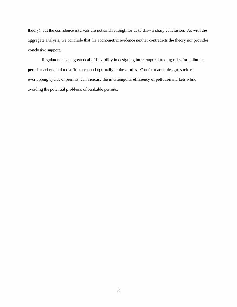
31
theory), but the confidence intervals are not small enough for us to draw a sharp conclusion. As with the
aggregate analysis, we conclude that the econometric evidence neither contradicts the theory nor provides
conclusive support.
Regulators have a great deal of flexibility in designing intertemporal trading rules for pollution
permit markets, and most firms respond optimally to these rules. Careful market design, such as
overlapping cycles of permits, can increase the intertemporal efficiency of pollution markets while
avoiding the potential problems of bankable permits.
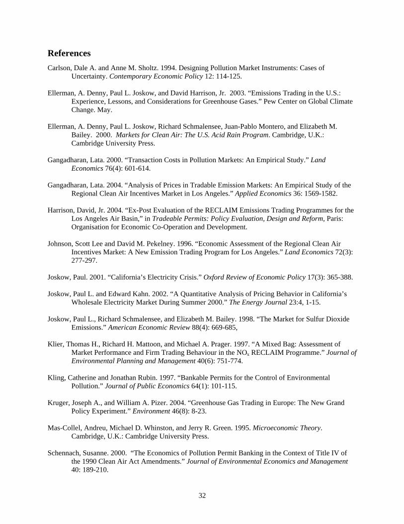
32
References Carlson, Dale A. and Anne M. Sholtz. 1994. Designing Pollution Market Instruments: Cases of
Uncertainty. Contemporary Economic Policy 12: 114-125. Ellerman, A. Denny, Paul L. Joskow, and David Harrison, Jr. 2003. “Emissions Trading in the U.S.:
Experience, Lessons, and Considerations for Greenhouse Gases.” Pew Center on Global Climate Change. May.
Ellerman, A. Denny, Paul L. Joskow, Richard Schmalensee, Juan-Pablo Montero, and Elizabeth M.
Bailey. 2000. Markets for Clean Air: The U.S. Acid Rain Program. Cambridge, U.K.: Cambridge University Press.
Gangadharan, Lata. 2000. “Transaction Costs in Pollution Markets: An Empirical Study.” Land
Economics 76(4): 601-614. Gangadharan, Lata. 2004. “Analysis of Prices in Tradable Emission Markets: An Empirical Study of the
Regional Clean Air Incentives Market in Los Angeles.” Applied Economics 36: 1569-1582. Harrison, David, Jr. 2004. “Ex-Post Evaluation of the RECLAIM Emissions Trading Programmes for the
Los Angeles Air Basin,” in Tradeable Permits: Policy Evaluation, Design and Reform, Paris: Organisation for Economic Co-Operation and Development.
Johnson, Scott Lee and David M. Pekelney. 1996. “Economic Assessment of the Regional Clean Air
Incentives Market: A New Emission Trading Program for Los Angeles.” Land Economics 72(3): 277-297.
Joskow, Paul. 2001. “California’s Electricity Crisis.” Oxford Review of Economic Policy 17(3): 365-388. Joskow, Paul L. and Edward Kahn. 2002. “A Quantitative Analysis of Pricing Behavior in California’s
Wholesale Electricity Market During Summer 2000.” The Energy Journal 23:4, 1-15. Joskow, Paul L., Richard Schmalensee, and Elizabeth M. Bailey. 1998. “The Market for Sulfur Dioxide
Emissions.” American Economic Review 88(4): 669-685, Klier, Thomas H., Richard H. Mattoon, and Michael A. Prager. 1997. “A Mixed Bag: Assessment of
Market Performance and Firm Trading Behaviour in the NOx RECLAIM Programme.” Journal of Environmental Planning and Management 40(6): 751-774.
Kling, Catherine and Jonathan Rubin. 1997. “Bankable Permits for the Control of Environmental
Pollution.” Journal of Public Economics 64(1): 101-115. Kruger, Joseph A., and William A. Pizer. 2004. “Greenhouse Gas Trading in Europe: The New Grand
Policy Experiment.” Environment 46(8): 8-23. Mas-Collel, Andreu, Michael D. Whinston, and Jerry R. Green. 1995. Microeconomic Theory.
Cambridge, U.K.: Cambridge University Press. Schennach, Susanne. 2000. “The Economics of Pollution Permit Banking in the Context of Title IV of
the 1990 Clean Air Act Amendments.” Journal of Environmental Economics and Management 40: 189-210.
33
Schwarze, Reimund and Peter Zapfel. 2000. “Sulfur Allowance Trading and the Regional Clean Air
Incentives Market: A Comparative Design Analysis of Two Major Cap-and-Trade Permit Programs.” Environmental and Resource Economics 17: 279-298.
South Coast Air Quality Management District. 2007a. Annual RECLAIM Audit Report for the 2005
Compliance Year. March 2. South Coast Air Quality Management District. 2007b. Regulation XX: Regional Clean Air Incentives
Market (RECLAIM), http://www.aqmd.gov/rules/reg/reg20_tofc.html, accessed July 16, 2007. Stavins, Robert N. 1998. “What Can We Learn from the Grand Policy Experiment? Lessons from SO2
Allowance Trading.” Journal of Economic Perspectives 12(3): 69-88. Tietenberg, Thomas H. 2006. Emissions Trading: Principles and Practice. Washington, D.C.: Resources
for the Future. USEPA. 2002. “An Evaluation of the South Coast Air Quality District’s Regional Clean Air Incentives
Market – Lessons in Environmental Markets and Innovation.” November http://www.epa.gov/region09/air/reclaim/report.pdf.
USEPA. 2006. “An Overview of the Regional Clean Air Incentives Market (RECLAIM),” Staff Paper,
EPA Clean Air Markets Division, August 14. USEPA. 2007. Green Book: Nonattainment Areas for Criteria Pollutants
http://www.epa.gov/air/oaqps/greenbk/index.html, accessed July 16, 2007. Yates, Andrew J. and Mark B. Cronshaw. 2001. “Pollution Permit Markets with Intertemporal Trading
and Asymmetric Information.” Journal of Environmental Economics and Management 42, 104–118.
34
0
10,000
20,000
30,000
40,000
50,00019
94
1995
1996
1997
1998
1999
2000
2001
2002
2003
2004
2005
Initial Allocation Available RTCs Used RTCs
Figure 1. Initial allocations, available RTCs, and used RTCs for permits expiring in June or December of each year from December 1994 to June 2006. Thousands of RTCs.
0
0.2
0.4
0.6
0.8
1
1.2
1.4
1.6
1.8
2
1 2 3 4 5 6 7 8 9 10 11 12 13 14 15 16
quarter
pric
e
p4p6p8p10p12p14p16
Figure 2: Steady-state equilibrium permit prices. The permits of each vintage are exhausted in
their first two quarters of validity. Prices are circled for which there is positive demand.

35
0
0.2
0.4
0.6
0.8
1
1.2
1.4
1.6
1.8
1 2 3 4 5 6 7 8 9 10 11 12 13 14 15 16
quarter
Pric
e
p4p6p8p10p12p14p16
Figure 3: Equilibrium permit prices with larger decrease in endowment of permits beginning,
with those expiring in quarter 10. The present values of permits expiring in quarters 8 and 10 are equal.
0
0.05
0.1
0.15
0.2
0.25
1 2 3 4 5 6 7 8 9 10 11 12 13 14 15 16
quarter
Pric
e
p4p6p8p10p12p14p16
Figure 4: Equilibrium permit prices with change from zero price to positive price. Some of the
p6 permits are “banked” while some of the p14 permits are “borrowed.”
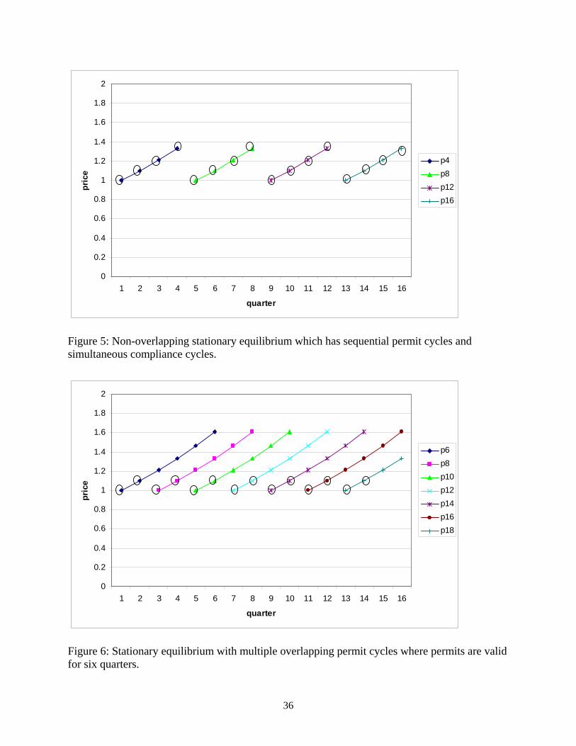
36
0
0.2
0.4
0.6
0.8
1
1.2
1.4
1.6
1.8
2
1 2 3 4 5 6 7 8 9 10 11 12 13 14 15 16
quarter
pric
e
p4p8p12p16
Figure 5: Non-overlapping stationary equilibrium which has sequential permit cycles and simultaneous compliance cycles.
0
0.2
0.4
0.6
0.8
1
1.2
1.4
1.6
1.8
2
1 2 3 4 5 6 7 8 9 10 11 12 13 14 15 16
quarter
pric
e
p6p8p10p12p14p16p18
Figure 6: Stationary equilibrium with multiple overlapping permit cycles where permits are valid for six quarters.
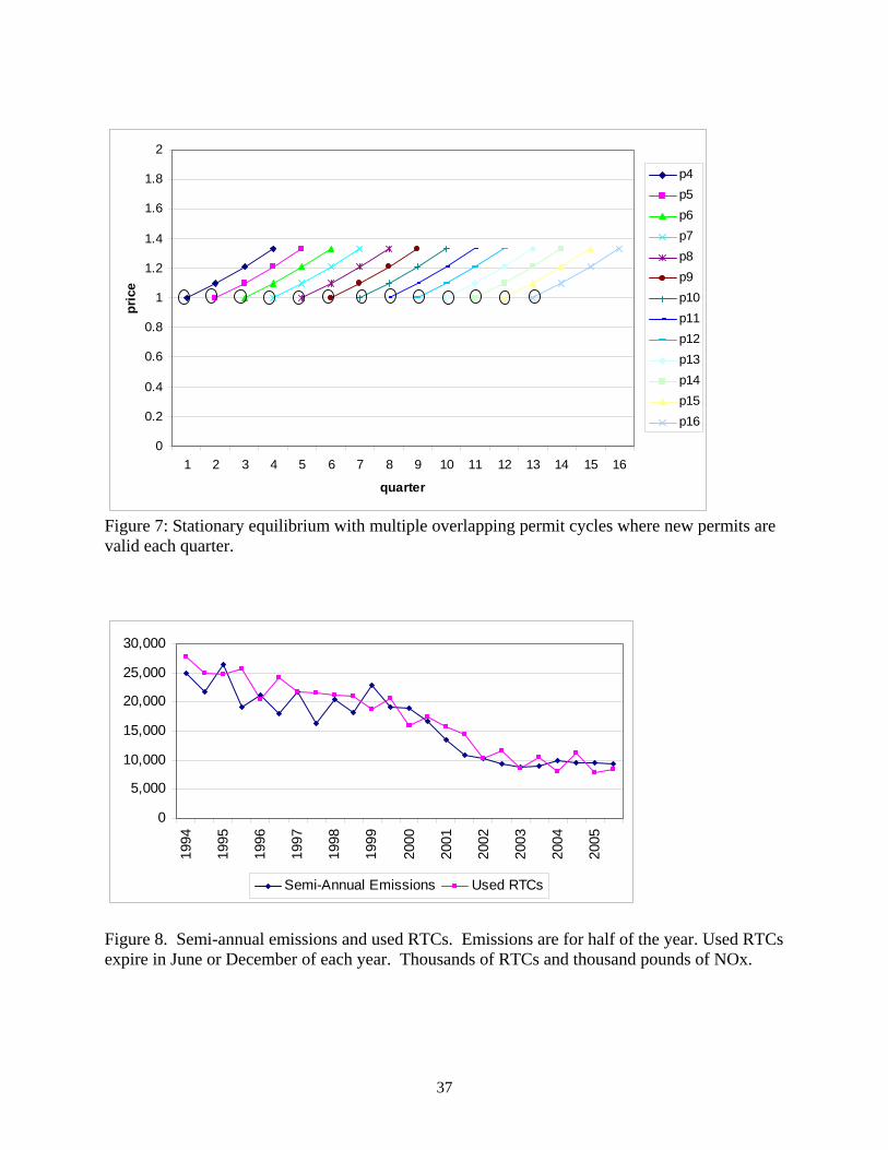
37
0
0.2
0.4
0.6
0.8
1
1.2
1.4
1.6
1.8
2
1 2 3 4 5 6 7 8 9 10 11 12 13 14 15 16
quarter
pric
e
p4p5p6p7p8p9p10p11p12p13p14p15p16
Figure 7: Stationary equilibrium with multiple overlapping permit cycles where new permits are valid each quarter.
0
5,000
10,000
15,000
20,000
25,000
30,000
1994
1995
1996
1997
1998
1999
2000
2001
2002
2003
2004
2005
Semi-Annual Emissions Used RTCs
Figure 8. Semi-annual emissions and used RTCs. Emissions are for half of the year. Used RTCs expire in June or December of each year. Thousands of RTCs and thousand pounds of NOx.
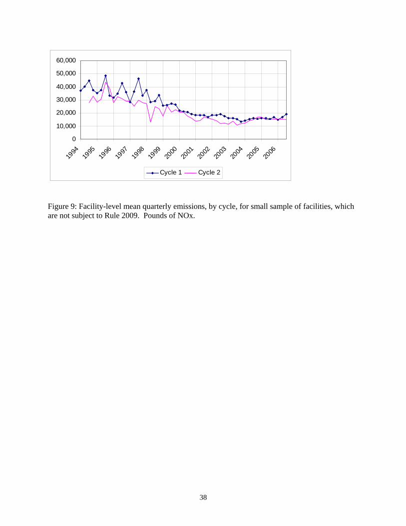
38
0
10,000
20,000
30,000
40,000
50,000
60,000
1994
1995
1996
1997
1998
1999
2000
2001
2002
2003
2004
2005
2006
Cycle 1 Cycle 2
Figure 9: Facility-level mean quarterly emissions, by cycle, for small sample of facilities, which are not subject to Rule 2009. Pounds of NOx.
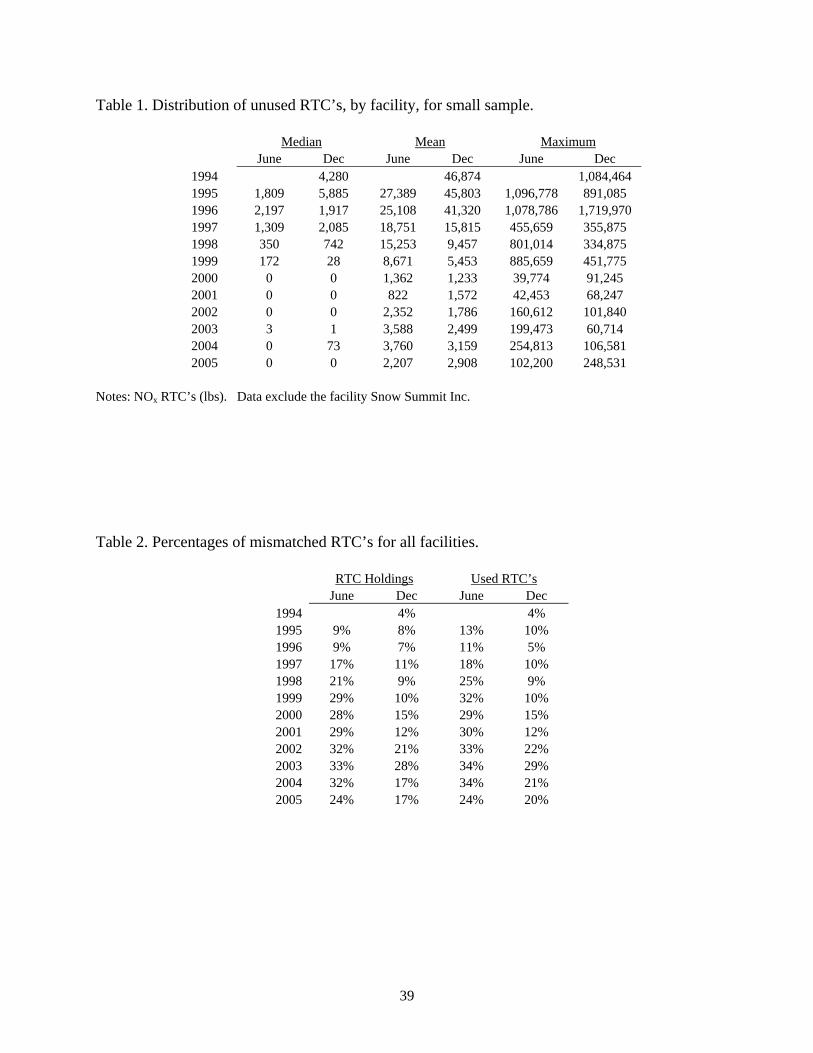
39
Table 1. Distribution of unused RTC’s, by facility, for small sample.
Median Mean Maximum June Dec June Dec June Dec
1994 4,280 46,874 1,084,464 1995 1,809 5,885 27,389 45,803 1,096,778 891,085 1996 2,197 1,917 25,108 41,320 1,078,786 1,719,970 1997 1,309 2,085 18,751 15,815 455,659 355,875 1998 350 742 15,253 9,457 801,014 334,875 1999 172 28 8,671 5,453 885,659 451,775 2000 0 0 1,362 1,233 39,774 91,245 2001 0 0 822 1,572 42,453 68,247 2002 0 0 2,352 1,786 160,612 101,840 2003 3 1 3,588 2,499 199,473 60,714 2004 0 73 3,760 3,159 254,813 106,581 2005 0 0 2,207 2,908 102,200 248,531
Notes: NOx RTC’s (lbs). Data exclude the facility Snow Summit Inc. Table 2. Percentages of mismatched RTC’s for all facilities.
RTC Holdings Used RTC’s June Dec June Dec
1994 4% 4% 1995 9% 8% 13% 10% 1996 9% 7% 11% 5% 1997 17% 11% 18% 10% 1998 21% 9% 25% 9% 1999 29% 10% 32% 10% 2000 28% 15% 29% 15% 2001 29% 12% 30% 12% 2002 32% 21% 33% 22% 2003 33% 28% 34% 29% 2004 32% 17% 34% 21% 2005 24% 17% 24% 20%
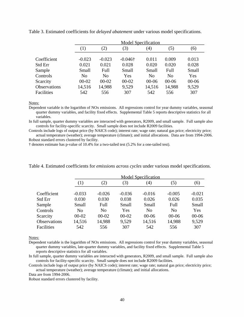
40
Table 3. Estimated coefficients for delayed abatement under various model specifications.
Model Specification (1) (2) (3) (4) (5) (6)
Coefficient -0.023 -0.023 -0.046† 0.011 0.009 0.013 Std Err 0.021 0.021 0.028 0.020 0.020 0.028 Sample Small Full Small Small Full Small Controls No No Yes No No Yes Scarcity 00-02 00-02 00-02 00-06 00-06 00-06 Observations 14,516 14,988 9,529 14,516 14,988 9,529 Facilities 542 556 307 542 556 307
Notes: Dependent variable is the logarithm of NOx emissions. All regressions control for year dummy variables, seasonal
quarter dummy variables, and facility fixed effects. Supplemental Table 5 reports descriptive statistics for all variables.
In full sample, quarter dummy variables are interacted with generators, R2009, and small sample. Full sample also controls for facility-specific scarcity. Small sample does not include R2009 facilities.
Controls include logs of output price (by NAICS code); interest rate; wage rate; natural gas price; electricity price; actual temperature (weather); average temperature (climate); and initial allocations. Data are from 1994-2006.
Robust standard errors clustered by facility. † denotes estimate has p-value of 10.4% for a two-tailed test (5.2% for a one-tailed test). Table 4. Estimated coefficients for emissions across cycles under various model specifications.
Model Specification (1) (2) (3) (4) (5) (6)
Coefficient -0.033 -0.026 -0.036 -0.016 -0.005 -0.021 Std Err 0.030 0.030 0.038 0.026 0.026 0.035 Sample Small Full Small Small Full Small Controls No No Yes No No Yes Scarcity 00-02 00-02 00-02 00-06 00-06 00-06 Observations 14,516 14,988 9,529 14,516 14,988 9,529 Facilities 542 556 307 542 556 307
Notes: Dependent variable is the logarithm of NOx emissions. All regressions control for year dummy variables, seasonal
quarter dummy variables, late-quarter dummy variables, and facility fixed effects. Supplemental Table 5 reports descriptive statistics for all variables.
In full sample, quarter dummy variables are interacted with generators, R2009, and small sample. Full sample also controls for facility-specific scarcity. Small sample does not include R2009 facilities.
Controls include logs of output price (by NAICS code); interest rate; wage rate; natural gas price; electricity price; actual temperature (weather); average temperature (climate); and initial allocations.
Data are from 1994-2006. Robust standard errors clustered by facility.

41
Supplementary Material Appendix A: Extending the Model to Uncertain Abatement Costs Uncertainty plays an important role in pollution permit markets.42 To incorporate uncertainty in the preceding model, we focus on abatement cost shocks.43 The stochastic dynamic programming model has a value function in each quarter t, tV , and a separate value function for each compliance period, tW for t a multiple of four. The value functions, tV and tW , are functions of the entire vector of abatement in all preceding quarters. Assume the abatement cost shock is realized at the beginning of the period so that all preceding shocks are realized before the compliance period. Further assume the realized shocks are known by all market participants and the prices are revealed at the compliance period so there is no asymmetric information. For a facility in Cycle A, the Bellman equations for the firm’s optimization can then be written: [A1] }3,2,1{in)4,mod(for)(min 1 tVEacV ttttat
t++= δ
[A2] 0)4,mod(for)(min =+= tWEacV ttttatt
[A3]
0)4,mod(for)()()(min 122
12
12322
23
2 =++++++++= +++
−+
−−−−−
−−
− tVEddpddddpddpW tttt
tt
tt
tt
tt
tt
tt
tt
tt
tt
tt
ddt l
ikj
δ
where xt =)4,mod( means that xt − is a multiple of four and tE is the expectations operator at quarter t. Equations [A1] and [A2] show that the optimized value function in each quarter minimizes the costs of abatement plus the expected continuation based on current information. For the first three quarters of the compliance year, see [A1], the continuation is another quarter with (discounted and uncertain) abatement costs. After the fourth quarter, see [A2], the continuation is to the compliance period where prices are revealed. In the compliance period (in [A3] where t is a multiple of four), the firm chooses whether to use permits of cycle A or cycle B to cover its required emissions for each quarter. Note that the optimization in [A3] is subject to the identity jit
tit
ttt dda +++ −−=ε for every t. The continuation from the compliance period is then another quarter with (discounted and uncertain) abatement costs. To illustrate the dynamic program, first consider the compliance period. Since the objective is linear in the controls, the solution will always be a corner solution and the optimized value will be the minimum of the two prices. Equation [A3] then becomes
122
112
2322
23
2 )}(,min{)}(,min{ +++
−−+
−−−−
−−
− ++++++++= tttt
tt
tt
tt
tt
tt
tt
tt
tt
tt
tt
ttt VEddddppddddppW δ
which is equivalently [A4] 111
22233
2 )}(,min{)}(,min{ +−−+
−−−−− +−+−+−+−= tttttt
tt
tttttt
tt
ttt VEaappaappW δεεεε
using the identity jitt
itttt dda +++ −−=ε . Equation [A4] implies that the optimized value in the compliance
period is the minimum price times emissions for each of the four quarters plus the continuation. The first order condition for [A2] can be written
[A5] },min{)( 2+=∂∂
−=′ tt
ttt
t
tttt ppE
aW
Eac .
42 Yates and Cronshaw (2001) analyze intertemporal trading with uncertain abatement costs and show that bankable permits are preferred if marginal damages are relatively flat. 43 One can think of these as multiplicative shocks to the abatement cost function.
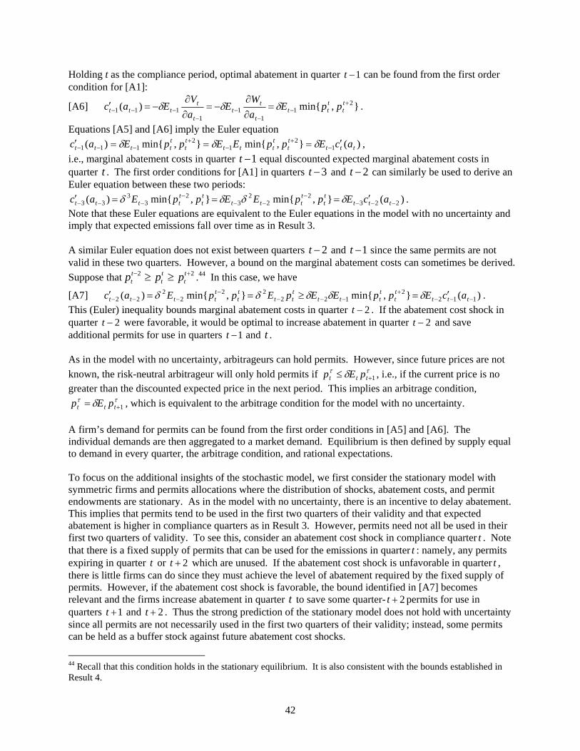
42
Holding t as the compliance period, optimal abatement in quarter 1−t can be found from the first order condition for [A1]:
[A6] },min{)( 21
11
1111
+−
−−
−−−− =
∂∂
−=∂∂
−=′ tt
ttt
t
tt
t
tttt ppE
aW
EaV
Eac δδδ .
Equations [A5] and [A6] imply the Euler equation )(},min{},min{)( 1
21
2111 ttt
tt
tttt
tt
ttttt acEppEEppEac ′===′ −
+−
+−−− δδδ ,
i.e., marginal abatement costs in quarter 1−t equal discounted expected marginal abatement costs in quarter t . The first order conditions for [A1] in quarters 3−t and 2−t can similarly be used to derive an Euler equation between these two periods:
)(},min{},min{)( 2232
22
32
33
33 −−−−
−−−
−−− ′===′ ttttt
tttt
tt
ttttt acEppEEppEac δδδδ .
Note that these Euler equations are equivalent to the Euler equations in the model with no uncertainty and imply that expected emissions fall over time as in Result 3. A similar Euler equation does not exist between quarters 2−t and 1−t since the same permits are not valid in these two quarters. However, a bound on the marginal abatement costs can sometimes be derived. Suppose that 22 +− ≥≥ t
ttt
tt ppp .44 In this case, we have
[A7] )(},min{},min{)( 1122
12222
22
22 −−−+
−−−−
−−− ′=≥==′ ttttt
tttt
ttt
tt
ttttt acEppEEpEppEac δδδδδ .
This (Euler) inequality bounds marginal abatement costs in quarter 2−t . If the abatement cost shock in quarter 2−t were favorable, it would be optimal to increase abatement in quarter 2−t and save additional permits for use in quarters 1−t and t . As in the model with no uncertainty, arbitrageurs can hold permits. However, since future prices are not known, the risk-neutral arbitrageur will only hold permits if ττ δ 1+≤ ttt pEp , i.e., if the current price is no greater than the discounted expected price in the next period. This implies an arbitrage condition,
ττ δ 1+= ttt pEp , which is equivalent to the arbitrage condition for the model with no uncertainty. A firm’s demand for permits can be found from the first order conditions in [A5] and [A6]. The individual demands are then aggregated to a market demand. Equilibrium is then defined by supply equal to demand in every quarter, the arbitrage condition, and rational expectations. To focus on the additional insights of the stochastic model, we first consider the stationary model with symmetric firms and permits allocations where the distribution of shocks, abatement costs, and permit endowments are stationary. As in the model with no uncertainty, there is an incentive to delay abatement. This implies that permits tend to be used in the first two quarters of their validity and that expected abatement is higher in compliance quarters as in Result 3. However, permits need not all be used in their first two quarters of validity. To see this, consider an abatement cost shock in compliance quarter t . Note that there is a fixed supply of permits that can be used for the emissions in quarter t : namely, any permits expiring in quarter t or 2+t which are unused. If the abatement cost shock is unfavorable in quarter t , there is little firms can do since they must achieve the level of abatement required by the fixed supply of permits. However, if the abatement cost shock is favorable, the bound identified in [A7] becomes relevant and the firms increase abatement in quarter t to save some quarter- 2+t permits for use in quarters 1+t and 2+t . Thus the strong prediction of the stationary model does not hold with uncertainty since all permits are not necessarily used in the first two quarters of their validity; instead, some permits can be held as a buffer stock against future abatement cost shocks.
44 Recall that this condition holds in the stationary equilibrium. It is also consistent with the bounds established in Result 4.
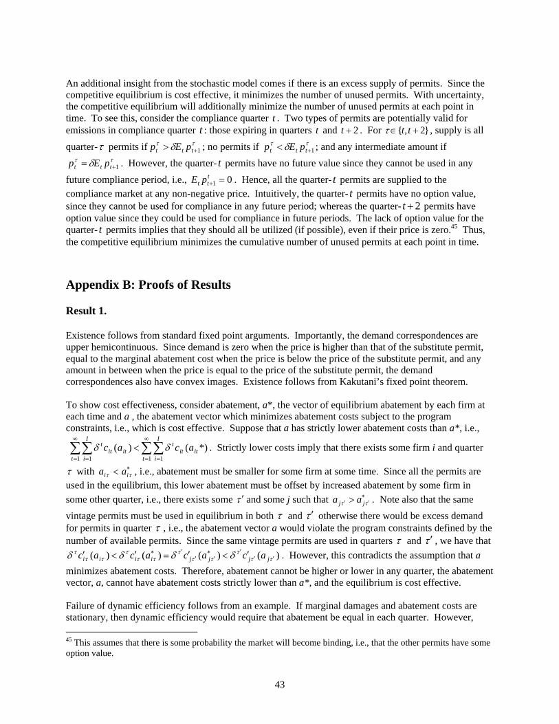
43
An additional insight from the stochastic model comes if there is an excess supply of permits. Since the competitive equilibrium is cost effective, it minimizes the number of unused permits. With uncertainty, the competitive equilibrium will additionally minimize the number of unused permits at each point in time. To see this, consider the compliance quarter t . Two types of permits are potentially valid for emissions in compliance quarter t : those expiring in quarters t and 2+t . For }2,{ +∈ ttτ , supply is all
quarter-τ permits if ττ δ 1+> ttt pEp ; no permits if ττ δ 1+< ttt pEp ; and any intermediate amount if ττ δ 1+= ttt pEp . However, the quarter- t permits have no future value since they cannot be used in any
future compliance period, i.e., 01 =+ttt pE . Hence, all the quarter- t permits are supplied to the
compliance market at any non-negative price. Intuitively, the quarter- t permits have no option value, since they cannot be used for compliance in any future period; whereas the quarter- 2+t permits have option value since they could be used for compliance in future periods. The lack of option value for the quarter- t permits implies that they should all be utilized (if possible), even if their price is zero.45 Thus, the competitive equilibrium minimizes the cumulative number of unused permits at each point in time. Appendix B: Proofs of Results Result 1. Existence follows from standard fixed point arguments. Importantly, the demand correspondences are upper hemicontinuous. Since demand is zero when the price is higher than that of the substitute permit, equal to the marginal abatement cost when the price is below the price of the substitute permit, and any amount in between when the price is equal to the price of the substitute permit, the demand correspondences also have convex images. Existence follows from Kakutani’s fixed point theorem. To show cost effectiveness, consider abatement, a*, the vector of equilibrium abatement by each firm at each time and a , the abatement vector which minimizes abatement costs subject to the program constraints, i.e., which is cost effective. Suppose that a has strictly lower abatement costs than a*, i.e.,
∑∑∑∑∞
= =
∞
= =
<1 11 1
*)()(t
I
iitit
t
t
I
iitit
t acac δδ . Strictly lower costs imply that there exists some firm i and quarter
τ with ∗< ττ ii aa , i.e., abatement must be smaller for some firm at some time. Since all the permits are used in the equilibrium, this lower abatement must be offset by increased abatement by some firm in some other quarter, i.e., there exists some τ ′ and some j such that ∗
′′ > ττ jj aa . Note also that the same vintage permits must be used in equilibrium in both τ and τ ′ otherwise there would be excess demand for permits in quarter τ , i.e., the abatement vector a would violate the program constraints defined by the number of available permits. Since the same vintage permits are used in quarters τ and τ ′ , we have that
)()()()( τττ
τττ
τττ
τττ δδδδ ′′
′∗′′
′∗ ′<′=′<′ jjjjiiii acacacac . However, this contradicts the assumption that a minimizes abatement costs. Therefore, abatement cannot be higher or lower in any quarter, the abatement vector, a, cannot have abatement costs strictly lower than a*, and the equilibrium is cost effective. Failure of dynamic efficiency follows from an example. If marginal damages and abatement costs are stationary, then dynamic efficiency would require that abatement be equal in each quarter. However, 45 This assumes that there is some probability the market will become binding, i.e., that the other permits have some option value.

44
from the first order conditions for quarters 1 and 2, we see that )(},min{)( 222
444
41 acppac ′==′ δδδ which
implies that 21 aa < . Result 2. a) Merging two firms i and j give the new abatement cost function: )()()( tjtjtititjtit acacaaC +=+ since there are no cost externalities across facilities. The merged firm minimizes abatement costs by setting },min{)( 00
jitittjtit
t ppaaC +++=+′δ and by setting )()()( tjtjtititjtit acacaaC ′=′=+′ . But this is equivalent to [5] for both unmerged firms. b) A firm in cycle A would abate such that },min{)( 00
jitittt
t ppac +++=′δ in quarter t. The firm would face exactly the same two prices if it were in cycle B. c) Since the abatement condition },min{)( 00
jitittt
t ppac +++=′δ does not depend on the initial endowment, reallocating the initial endowment does not affect emissions as long as the aggregate allotment remains unchanged. d) Here we analyze the effects of requiring quarterly compliance rather than annual compliance. The cycle A firm’s optimization is
[B1] ∑∞
=
++++++ +++++
1)(min
t
jitt
jitt
titt
itt
tAt
At
t
dddpdpac
jitt
itt
δδδ .
The Kuhn-Tucker first order conditions together with the arbitrage condition imply
},min{},min{)( 00jititjit
tit
ttA
tA
tt ppppac ++++++ ==′ δδ . This condition is identical to the condition in [5].
Thus the equilibrium is invariant to requiring quarterly compliance. The intuition lies with the arbitrage condition. Firms discount the price they will pay for permits based on how far in the future compliance occurs. The intertemporal arbitrage condition implies that the present value permit price is always equal, and thus the equilibrium is invariant to whether compliance occurs immediately or in the distant future. Result 3. Since t is a compliance quarter, },min{)( 00
jitittt
t ppac +++=′δ and },min{)( 00111 jitit
ttt ppac +++
−−− =′δ . But
this implies that )()( 1 tt acac ′=′ − δ , which implies that )()( 1 tt acac ′<′ − and tt aa <−1 . Result 4. The first part of Result 4 follows because aggregate demand for permits of each cycle must be positive in equilibrium. In the first half of the compliance year, firms can use permits expiring in 2−t or t . If permits expiring in 2−t were cheaper, then demand for permits expiring in t would be zero for the first two quarters. Similarly, in the second half of the compliance year, firms use the cheaper of permits expiring in t or 2+t . Thus if },max{ 2
02
00+−> ttt ppp demand would be zero. The second part of Result
4 follows because if the condition holds, then firms of both cycles would demand only permits expiring in t . This can only occur in equilibrium if there are sufficient permits to cover emissions from all firms in both cycles.
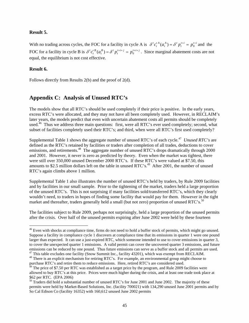
45
Result 5. With no trading across cycles, the FOC for a facility in cycle A is itit
ttA
tA
tt ppac ++ ==′ 0)( δδ and the
FOC for a facility in cycle B is jitjitt
tBt
Bt
t ppac ++++ ==′ 0)( δδ . Since marginal abatement costs are not equal, the equilibrium is not cost effective. Result 6. Follows directly from Results 2(b) and the proof of 2(d). Appendix C: Analysis of Unused RTC’s The models show that all RTC’s should be used completely if their price is positive. In the early years, excess RTC’s were allocated, and they may not have all been completely used. However, in RECLAIM’s later years, the models predict that even with uncertain abatement costs all permits should be completely used.46 Thus we address three main questions: first, were all RTC’s ever used completely; second, what subset of facilities completely used their RTC’s; and third, when were all RTC’s first used completely? Supplemental Table 1 shows the aggregate number of unused RTC’s of each cycle.47 Unused RTC’s are defined as the RTC’s retained by facilities or traders after completion of all trades, deductions to cover emissions, and retirements.48 The aggregate number of unused RTC’s drops dramatically through 2000 and 2001. However, it never is zero as predicted by theory. Even when the market was tightest, there were still over 350,000 unused December 2000 RTC’s. If these RTC’s were valued at $7.50, this amounts to $2.5 million dollars left on the table in unused RTC’s.49 After 2001, the number of unused RTC’s again climbs above 1 million. Supplemental Table 1 also illustrates the number of unused RTC’s held by traders, by Rule 2009 facilities and by facilities in our small sample. Prior to the tightening of the market, traders held a large proportion of the unused RTC’s. This is not surprising if many facilities sold/transferred RTC’s, which they clearly wouldn’t need, to traders in hopes of finding some facility that would pay for them. However in the tight market and thereafter, traders generally held a small (but not zero) proportion of unused RTC’s.50 The facilities subject to Rule 2009, perhaps not surprisingly, held a large proportion of the unused permits after the crisis. Over half of the unused permits expiring after June 2002 were held by these fourteen
46 Even with shocks at compliance time, firms do not need to hold a buffer stock of permits, which might go unused. Suppose a facility in compliance cycle 1 discovers at compliance time that its emissions in quarter 1 were one pound larger than expected. It can use a just-expired RTC, which someone intended to use to cover emissions in quarter 3, to cover the unexpected quarter 1 emissions. A valid permit can cover the uncovered quarter 3 emissions, and future emissions can be reduced by one pound. Thus future emissions can serve as a buffer stock and all permits are used. 47 This table excludes one facility (Snow Summit Inc., facility 43201), which was exempt from RECLAIM. 48 There is an explicit mechanism for retiring RTC’s. For example, an environmental group might choose to purchase RTC’s and retire them to reduce emissions. Here, retired RTC’s are considered used. 49 The price of $7.50 per RTC was established as a target price by the program, and Rule 2009 facilities were allowed to buy RTC’s at this price. Prices were much higher during the crisis, and at least one trade took place at $62 per RTC. (EPA 2006) 50 Traders did hold a substantial number of unused RTC’s for June 2001 and June 2002. The majority of these permits were held by Market-Based Solutions, Inc. (facility 700021) with 134,290 unused June 2001 permits and by So Cal Edison Co (facility 16352) with 160,612 unused June 2002 permits

46
facilities. (Supplemental Tables 2 and 3 list the electricity generators and facilities subject to Rule 2009.) For the remaining facilities, those in the small sample category, there was no prohibition against trading. However, these facilities continued to hold a significant number of unused permits. To summarize, facilities hold unused RTC’s, many of which can be explained by the excess initial allocations in RECLAIM’s early years or by the market segmentation in response to the crisis. On the other hand, a substantial proportion of the facilities not subject to trading prohibitions had no unused RTC’s: over forty percent had zero unused RTC’s expiring after 1999. This suggests that the facilities not subject to trading restrictions (although not all such facilities) were using all RTC’s, as predicted by theory. Supplemental Table 1. Total unused RTC’s held by traders, R2009 facilities, and small sample.
All Facilities and
Traders Traders R2009 Facilities Sample June Dec June Dec June Dec June Dec 1994 22,661 12,413 1,028 9,609 1995 17,856 18,993 9,780 6,823 600 1,886 7,833 10,672 1996 12,306 16,212 4,522 4,207 589 1,605 7,307 10,413 1997 8,028 5,142 2,035 272 92 981 5,963 3,891 1998 6,680 3,961 1,618 828 56 676 5,049 2,468 1999 3,453 1,906 156 3 272 376 3,043 1,527 2000 494 358 45 3 14 0 477 358 2001 462 521 173 16 1 18 308 498 2002 1,053 929 213 106 90 306 953 522 2003 1,573 2,577 122 63 134 1,798 1,374 732 2004 2,447 3,303 67 130 949 2,202 1,470 976 2005 1,708 3,398 14 122 833 2,372 874 922
Notes: Thousands of NOx RTC’s (lbs). “June” (“December”) represents RTC’s expiring in June (December). Data exclude the facility Snow Summit Inc. Supplemental Table 2: Electricity generators. Generators AES (4), Alliance Colton (2), Arco, Berry Petroleum, Burbank City, Carson Cogen (3), CES Energy, City of Anaheim, El Segundo, LADWP (4), Long Beach, Mountainview (2), NP Cogen, OLS Energy-Chino, Pasadena City, Reliant, Riverside Canal, So Cal Edison (9), Sunlaw Cogen (2), Television City Cogen, Trigen- LA (2)
Supplemental Table 3: Facilities subject to Rule 2009. Rule 2009 AES (3), City Of Burbank, El Segundo Power, LADWP (4), Long Beach Generation, Mountain Vista, Mountainview, Pasadena City, Riverside Canal
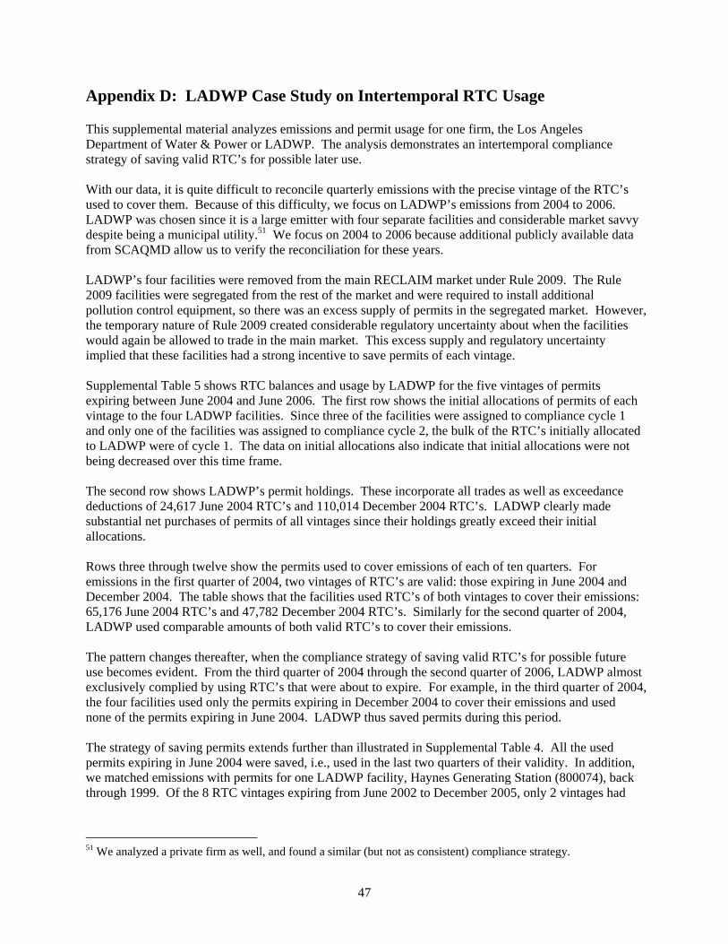
47
Appendix D: LADWP Case Study on Intertemporal RTC Usage This supplemental material analyzes emissions and permit usage for one firm, the Los Angeles Department of Water & Power or LADWP. The analysis demonstrates an intertemporal compliance strategy of saving valid RTC’s for possible later use. With our data, it is quite difficult to reconcile quarterly emissions with the precise vintage of the RTC’s used to cover them. Because of this difficulty, we focus on LADWP’s emissions from 2004 to 2006. LADWP was chosen since it is a large emitter with four separate facilities and considerable market savvy despite being a municipal utility.51 We focus on 2004 to 2006 because additional publicly available data from SCAQMD allow us to verify the reconciliation for these years. LADWP’s four facilities were removed from the main RECLAIM market under Rule 2009. The Rule 2009 facilities were segregated from the rest of the market and were required to install additional pollution control equipment, so there was an excess supply of permits in the segregated market. However, the temporary nature of Rule 2009 created considerable regulatory uncertainty about when the facilities would again be allowed to trade in the main market. This excess supply and regulatory uncertainty implied that these facilities had a strong incentive to save permits of each vintage. Supplemental Table 5 shows RTC balances and usage by LADWP for the five vintages of permits expiring between June 2004 and June 2006. The first row shows the initial allocations of permits of each vintage to the four LADWP facilities. Since three of the facilities were assigned to compliance cycle 1 and only one of the facilities was assigned to compliance cycle 2, the bulk of the RTC’s initially allocated to LADWP were of cycle 1. The data on initial allocations also indicate that initial allocations were not being decreased over this time frame. The second row shows LADWP’s permit holdings. These incorporate all trades as well as exceedance deductions of 24,617 June 2004 RTC’s and 110,014 December 2004 RTC’s. LADWP clearly made substantial net purchases of permits of all vintages since their holdings greatly exceed their initial allocations. Rows three through twelve show the permits used to cover emissions of each of ten quarters. For emissions in the first quarter of 2004, two vintages of RTC’s are valid: those expiring in June 2004 and December 2004. The table shows that the facilities used RTC’s of both vintages to cover their emissions: 65,176 June 2004 RTC’s and 47,782 December 2004 RTC’s. Similarly for the second quarter of 2004, LADWP used comparable amounts of both valid RTC’s to cover their emissions. The pattern changes thereafter, when the compliance strategy of saving valid RTC’s for possible future use becomes evident. From the third quarter of 2004 through the second quarter of 2006, LADWP almost exclusively complied by using RTC’s that were about to expire. For example, in the third quarter of 2004, the four facilities used only the permits expiring in December 2004 to cover their emissions and used none of the permits expiring in June 2004. LADWP thus saved permits during this period. The strategy of saving permits extends further than illustrated in Supplemental Table 4. All the used permits expiring in June 2004 were saved, i.e., used in the last two quarters of their validity. In addition, we matched emissions with permits for one LADWP facility, Haynes Generating Station (800074), back through 1999. Of the 8 RTC vintages expiring from June 2002 to December 2005, only 2 vintages had
51 We analyzed a private firm as well, and found a similar (but not as consistent) compliance strategy.
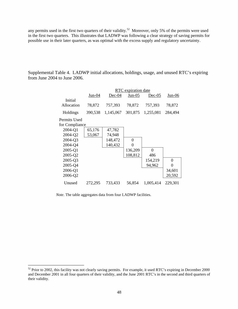
48
any permits used in the first two quarters of their validity.52 Moreover, only 5% of the permits were used in the first two quarters. This illustrates that LADWP was following a clear strategy of saving permits for possible use in their later quarters, as was optimal with the excess supply and regulatory uncertainty. Supplemental Table 4. LADWP initial allocations, holdings, usage, and unused RTC’s expiring from June 2004 to June 2006.
RTC expiration date Jun-04 Dec-04 Jun-05 Dec-05 Jun-06
Initial Allocation 78,872 757,393 78,872 757,393 78,872
Holdings 390,538 1,145,067 301,875 1,255,081 284,494
Permits Used for Compliance
2004-Q1 65,176 47,782 2004-Q2 53,067 74,948 2004-Q3 148,472 0 2004-Q4 140,432 0 2005-Q1 136,209 0 2005-Q2 108,812 486 2005-Q3 154,219 0 2005-Q4 94,962 0 2006-Q1 34,601 2006-Q2 20,592
Unused 272,295 733,433 56,854 1,005,414 229,301
Note. The table aggregates data from four LADWP facilities.
52 Prior to 2002, this facility was not clearly saving permits. For example, it used RTC’s expiring in December 2000 and December 2001 in all four quarters of their validity, and the June 2001 RTC’s in the second and third quarters of their validity.
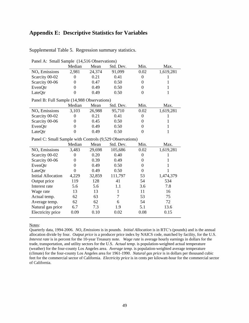
49
Appendix E: Descriptive Statistics for Variables Supplemental Table 5. Regression summary statistics. Panel A: Small Sample (14,516 Observations) Median Mean Std. Dev. Min. Max. NOx Emissions 2,981 24,374 91,099 0.02 1,619,281 Scarcity 00-02 0 0.21 0.41 0 1 Scarcity 00-06 0 0.47 0.50 0 1 EvenQtr 0 0.49 0.50 0 1 LateQtr 0 0.49 0.50 0 1
Panel B: Full Sample (14,988 Observations) Median Mean Std. Dev. Min. Max. NOx Emissions 3,103 26,988 95,710 0.02 1,619,281 Scarcity 00-02 0 0.21 0.41 0 1 Scarcity 00-06 0 0.45 0.50 0 1 EvenQtr 0 0.49 0.50 0 1 LateQtr 0 0.49 0.50 0 1
Panel C: Small Sample with Controls (9,529 Observations) Median Mean Std. Dev. Min. Max. NOx Emissions 3,483 29,698 105,686 0.02 1,619,281 Scarcity 00-02 0 0.20 0.40 0 1 Scarcity 00-06 0 0.39 0.49 0 1 EvenQtr 0 0.49 0.50 0 1 LateQtr 0 0.49 0.50 0 1 Initial Allocation 4,229 32,859 111,797 53 1,474,379 Output price 119 128 41 54 534 Interest rate 5.6 5.6 1.1 3.6 7.8 Wage rate 13 13 1 11 16 Actual temp. 62 63 7 53 75 Average temp. 62 62 6 54 72 Natural gas price 6.7 7.3 1.9 5.1 13.6 Electricity price 0.09 0.10 0.02 0.08 0.15
Notes: Quarterly data, 1994-2006. NOx Emissions is in pounds. Initial Allocation is in RTC’s (pounds) and is the annual allocation divide by four. Output price is a producer price index by NAICS code, matched by facility, for the U.S. Interest rate is in percent for the 10-year Treasury note. Wage rate is average hourly earnings in dollars for the trade, transportation, and utility sectors for the U.S. Actual temp. is population-weighted actual temperature (weather) for the four-county Los Angeles area. Average temp. is population-weighted average temperature (climate) for the four-county Los Angeles area for 1961-1990. Natural gas price is in dollars per thousand cubic feet for the commercial sector of California. Electricity price is in cents per kilowatt-hour for the commercial sector of California.