Steps for reduction of CCD images at CfA.  In the following computer output is in small type, prompts end with “:” or “>”, comments are in boldface, and what user types is in italics:

**You should read through "Jeannette Barnes: A Beginner's Guide to Using IRAF" (available athttp://iraf.noao.edu/docs/recommend.html) and use it as a reference while working through a reduction for the first few times.**

Ensure that all images are organized correctly. It is best to organize by image type (flats, darks, objects, bias etc) then further by any distinctions in those types, for example flats can be either dome or sky, and there can be more than one object, and each should be put into a separate object folder. Pay special attention to whether images have been taken using different set ups (i.e.different aperture's or filters) and divide accordingly.

For most steps IRAF overwrites the file that is being modified. Until you have all your files processed it is a good idea to save the output files of each step in a separate directory. Then if youfind an error you only have to go back to that saved file set and not start everything anew. If you do end up changing your working directory remember that some processes generate additional files that you will need. For example, the apall command generates a new folder called 'database' that lists the apertures. You will need a copy the database folder in addition to your images and flats for your next step.

Order of processing:1. Combine all bias files2. Subtract bias from all images3. Combine flats for a mean flatfield4. Normalize the mean flatfield5. Apply mean flatflied to all spectra6. Select object and sky regions and extract spectra7. Clean spectra of cosmic ray hits, etc.8. Calibrate pixel to wavelength using lamp lines

a) Extract comparison spectrab) Determine the comparison spectra dispersion solutionsc) Assign dispersion solutions to object spectrad) Apply dispersion solutions to object spectra

9.  Writing spectral files in ascii for input to molly and Doppler.10. Can convert to flux with standard stars but not necessary for tomography.

Use the following commands:

cl>hselect *fields to be extracted (EXPTYPE,EXPTIME,APERTURE,FILTER,OBJECT):

boolean expression governing selection (YES):

The hselect command allows you to pick out particular attributes from the image headers and displays them as a list, I have used the labels that appear on my headers but as they may differ  different sets of CCD's you may wish to perform cl>imhead [imagename] l+ to check for alternatelabels and use these in the "fields to be extracted" line.

1.  The first step in your actual reduction process is to combine bias frames together to form single zero frame for subtraction from images.

This step is performed via the zerocombine command, to access this IRAF tool proceed as follows:ecl> noao            artdata.        digiphot.     nobsolete.     onedspec.           astcat.           focas.          nproto.          rv.                 astrometry.   imred.         observatory   surfphot.           astutil.         mtlocal.       obsutil.          twodspec.  

noao> imred      argus.      crutil.     echelle.     iids.        kpnocoude.   specred.        bias.        ctioslit.   generic.    irred.      kpnoslit.        vtel.       ccdred.     dtoi.       hydra.       irs.          quadred.    

imred> ccdred      badpiximage       ccdmask             flatcombine       mkskyflat      ccdgroups           ccdproc              mkfringecor       setinstrument      ccdhedit              ccdtest                mkillumcor        zerocombine      ccdinstrument     combine             mkillumflat             ccdlist                 darkcombine       mkskycor   

**this brings you into the CCD reduction tools list where we will spend most of the time**  Note: if you are using fits files remember to set ccdtype to fits. Before actually running zerocombine we must check it's parameters using epar.  (Note that all tools are accessible after first call).

ccdred>epar zerocombine

  I R A F                      Image Reduction and Analysis FacilityPACKAGE = ccdred   TASK = zerocombine

input   =                       List of zero level images to combine(output =                 Zero) Output zero level name(combine=              median) Type of combine operation(reject =               ccdclip) Type of rejection

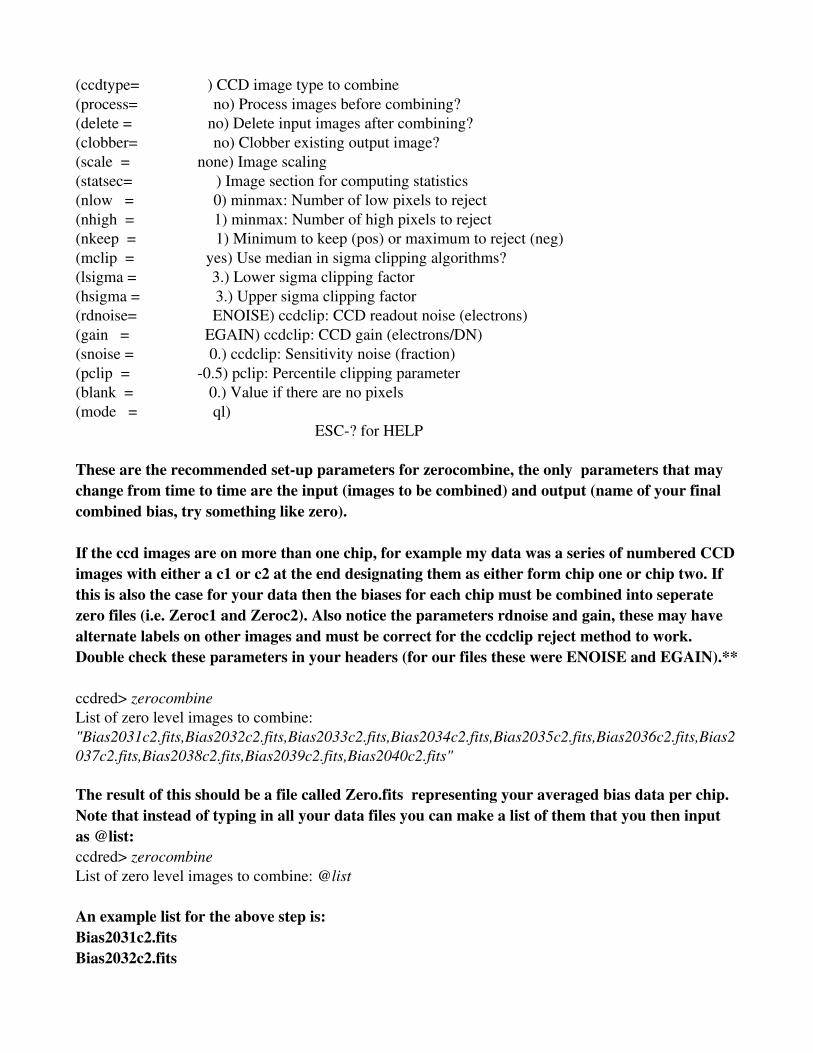
(ccdtype=                 ) CCD image type to combine(process=                   no) Process images before combining?(delete =                   no) Delete input images after combining?(clobber=                   no) Clobber existing output image?(scale  =                 none) Image scaling(statsec=                     ) Image section for computing statistics(nlow   =                    0) minmax: Number of low pixels to reject(nhigh  =                    1) minmax: Number of high pixels to reject(nkeep  =                    1) Minimum to keep (pos) or maximum to reject (neg)(mclip  =                  yes) Use median in sigma clipping algorithms?(lsigma =                   3.) Lower sigma clipping factor(hsigma =                   3.) Upper sigma clipping factor(rdnoise=                   ENOISE) ccdclip: CCD readout noise (electrons)(gain   =                   EGAIN) ccdclip: CCD gain (electrons/DN)(snoise =                   0.) ccdclip: Sensitivity noise (fraction)(pclip  =                 ­0.5) pclip: Percentile clipping parameter(blank  =                   0.) Value if there are no pixels(mode   =                   ql)                                                            ESC­? for HELP 

These are the recommended set­up parameters for zerocombine, the only  parameters that may change from time to time are the input (images to be combined) and output (name of your final combined bias, try something like zero).

If the ccd images are on more than one chip, for example my data was a series of numbered CCDimages with either a c1 or c2 at the end designating them as either form chip one or chip two. If this is also the case for your data then the biases for each chip must be combined into seperate zero files (i.e. Zeroc1 and Zeroc2). Also notice the parameters rdnoise and gain, these may have alternate labels on other images and must be correct for the ccdclip reject method to work.  Double check these parameters in your headers (for our files these were ENOISE and EGAIN).**

ccdred> zerocombineList of zero level images to combine: "Bias2031c2.fits,Bias2032c2.fits,Bias2033c2.fits,Bias2034c2.fits,Bias2035c2.fits,Bias2036c2.fits,Bias2037c2.fits,Bias2038c2.fits,Bias2039c2.fits,Bias2040c2.fits"

The result of this should be a file called Zero.fits  representing your averaged bias data per chip. Note that instead of typing in all your data files you can make a list of them that you then input as @list:ccdred> zerocombineList of zero level images to combine: @list

An example list for the above step is:Bias2031c2.fits    Bias2032c2.fits    

Bias2033c2.fits         Bias2034c2.fits Bias2035c2.fitsBias2036c2.fitsBias2037c2.fitsBias2038c2.fitsBias2039c2.fitsBias2040c2.fits

2. Removing the bias from the flats. 

Next prepare any flats for use in the rest of the reduction, copy the new zero combined files to thedirectories in which  each flat type is kept.  For this we will use ccdproc but we need to determinethe parameters that will be used as input.

A parameter called BIASSEC determines the overscan section of the image.  For a suitably large number of bias frames (at least 10) one does not need to have overscan active but if there are onlya few bias frames it is good to use this feature.

The parameter TRIMSEC is used to define useful area of the CCD chip.  Use an image of a flat todetermine the upper column cutoff and the range of lines for TRIMSEC.  In IRAF you need the implot command within plot.  Implot brings up a graphical interface and plots the middle line of your image to begin with, 

ccdred> plot      calcomp     gkidir      imdkern     phistogram  sgidecode   surface      contour     gkiextract  implot      pradprof    sgikern     velvect      crtpict     gkimosaic   nsppkern    prow        showcap           gdevices    graph       pcol        prows       stdgraph          gkidecode   hafton      pcols       pvector     stdplot     

plot> implotIf you haven't used the graphical interface before then check pages 27 onwards in the beginners manual.  A ? will list all the available keystroke commands for plotting.  For example typing (on the image):

:l 300   **will plot line 300**:c 200   **will plot column 200**also rather than checking each individual line you may want to have an average of a set of lines, which is a simple matter of typing :a xbefore typing :l or :c commands, it will average x number of lines/columns around the one you are trying to display and plot the average instead.  Type q on the plot to exit out of plot mode.

If you plot a line you will see a bit towards the right hand of the plot that goes essentially to zero counts: for a spectrum along the x­axis as we are using this as the lower limit of your BIASSEC, the upper limit is to the full range of the plot (you can figure this out by providing too large a column number to implot: it will just plot the last column instead and tell you its number); in thiscase 2048­2112.  The lines range will be the same for both biassec and trimsec. To determine line range plot any column of a flat file and then take the line range that contains your full slit; in thiscase 5­1000.  Now your biassec is [2048:2112,5:1000].  (Note when you want to actually extract a spectrum you may need to reduce the number of lines you use to the smallest possible that includes your science spectrum and a bit on either side to use for background subtraction. It is easiest to use ds9 to determine the limits: nominally about 60 lines should do this.  In this case we could use  the range from 590­650 so biassec is [2048:2112,590:650]. )   You can also use the full range  of acceptable lines now and determine the smaller extraction later: at that point you would need to use something other than ccdproc because ccdproc will only run a process throughonce.

For TRIMSEC use  the lower column limit of BIASSEC as your upper column limit; check an object image to look for  excess counts due to the chip edge; make this the lower limit of your trimsec.  In this case about 170.  Now your trimsec is [170:2048,590:650].  You should make sure that your trim region is the same for all your images: so use limits that avoid all chip edges.

Now check the parameters for ccdproc within ccdred (step by step instructions below)

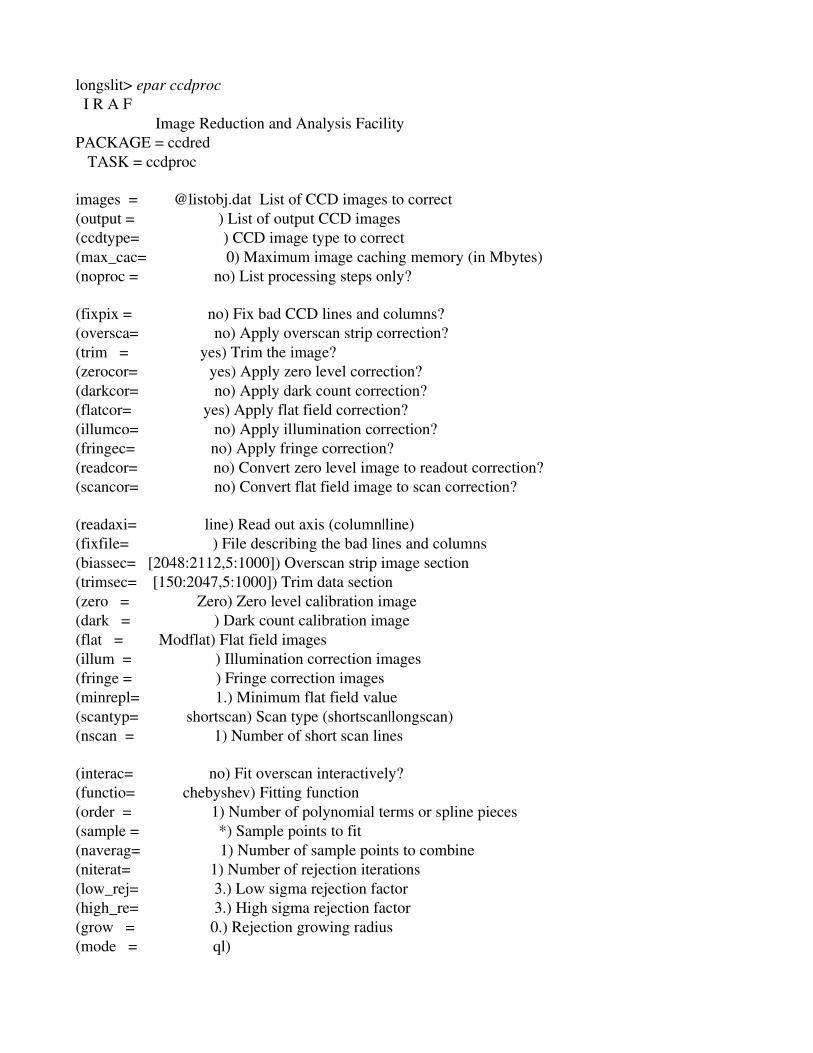
ccdred>epar ccdproc  

    I R A F                      Image Reduction and Analysis FacilityPACKAGE = ccdred   TASK = ccdprocimages  =                         List of CCD images to correct(output =                           ) List of output CCD images(ccdtype=                         ) CCD image type to correct(max_cac=                    0) Maximum image caching memory (in Mbytes)(noproc =                   no) List processing steps only?(fixpix =                   no) Fix bad CCD lines and columns?(oversca=                 no) Apply overscan strip correction?(trim   =                   yes) Trim the image?(zerocor=                 yes) Apply zero level correction?(darkcor=                  no) Aepapply dark count correction?(flatcor=                   no) Apply flat field correction?(illumco=                  no) Apply illumination correction?(fringec=                   no) Apply fringe correction?(readcor=                   no) Convert zero level image to readout correction?(scancor=                   no) Convert flat field image to scan correction?(readaxi=                  line) Read out axis (column|line)

(fixfile=                               ) File describing the bad lines and columns(biassec=           [2048:2112,5:1000]) Overscan strip image section(trimsec=             [150:2047,5:1000]) Trim data section(zero   =                         Zero) Zero level calibration image(dark   =                              ) Dark count calibration image(flat   =                                 ) Flat field images(illum  =                                ) Illumination correction images(fringe =                           ) Fringe correction images(minrepl=                   1.) Minimum flat field value(scantyp=                 shortscan) Scan type (shortscan|longscan)(nscan  =                        1) Number of short scan lines(interac=                   no) Fit overscan interactively?(functio=             chebyshev) Fitting function(order  =                    1) Number of polynomial terms or spline pieces(sample =                    *) Sample points to fit(naverag=                    1) Number of sample points to combine(niterat=                    1) Number of rejection iterations(low_rej=                   3.) Low sigma rejection factor(high_re=                   3.) High sigma rejection factor(grow   =                   0.) Rejection growing radius(mode   =                   ql)                                                            ESC­? for HELP Remember ctrl d to get out of parameter file with saved changes.

In addition to BIASSEC, TRIMSEC, and Zero file, the parameters you will need to change include:

images= the images you wish to process, as separate zero frames and flats exist for each chip you will want to process each chip image set separately.

output= as we will be processing large numbers of files leave this blank, note that this will result in old images being deleted once processed so BACK UP YOUR DATA!  (You could have an output list but that is somewhat dangerous as rewrites go to different names.)

ccdtype= leave this blank, as you have organized your data into separate folders this should be unnecessary.

**for this run we are only interested in having trim and zerocor on so everything else should remain as above.

Zero is the name of the combined bias file which corresponds to the image list, so if you are processing chip 1 images you would type zeroc1 into the zero section, and zeroc2 if  processing chip two. Make sure to change this for each chip.**

**Once prepared you are ready to perform a run of ccdproc.   Note ccdproc alters the header of 

images it has worked on so that it does not perform the same operations twice on the image when run again, it will only perform new processes which thus allows us to do things step by step***

ccdred> ccdprocList of CCD images to correct: @listflats.datccdred> 

**note if you have included oversca=yes you will recieve the following prompt Fit overscan vector for ccd0058c1.fits interactively (yes):You may wish to check how well the fitting is for the overscan by selecting yes the first time round, you will be presented with the overscan plot and a line that will try to best fit the large scale gradient of the data, you can change the order of the fit using :order x where  x is the order,and then pressing f to change the fit accordingly, but you should not need to exceed a straight linefit (order= 1 or 2) for most overscan data.  Once happy with the fit you can leave the graphical interface by pressing q and type NO (in caps) to apply your fit for all following images.**3.  Combining the flats

Now that we have prepared the flats we combine them into a single average flat.  It is sometimes a good idea to combine flats from several nights into a single Master flat, but if the flats themselves differ too much it is normally best to do a combined flat for each night.

For this use flatcombine,  for which the parameters should be as follows:

ccdred> epar flatcombine

                                   I R A F                      Image Reduction and Analysis FacilityPACKAGE = ccdred   TASK = flatcombine

input   =                       List of flat field images to combine(output =                 Flat) Output flat field root name(combine=              median) Type of combine operation(reject =            ccdclip) Type of rejection(ccdtype=                 ) CCD image type to combine(process=                  no) Process images before combining?(subsets=                  yes) Combine images by subset parameter?(delete =                   no) Delete input images after combining?(clobber=                   no) Clobber existing output image?(scale  =                 mode) Image scaling(statsec=                     ) Image section for computing statistics(nlow   =                    1) minmax: Number of low pixels to reject(nhigh  =                    1) minmax: Number of high pixels to reject(nkeep  =                    1) Minimum to keep (pos) or maximum to reject (neg)(mclip  =                  yes) Use median in sigma clipping algorithms?

(lsigma =                   3.) Lower sigma clipping factor(hsigma =                   3.) Upper sigma clipping factor(rdnoise=                   ENOISE) ccdclip: CCD readout noise (electrons)(gain   =                   EGAIN) ccdclip: CCD gain (electrons/DN)(snoise =                   0.) ccdclip: Sensitivity noise (fraction)(pclip  =                 ­0.5) pclip: Percentile clipping parameter(blank  =                   1.) Value if there are no pixels(mode   =                   ql)

** This is very similar to zerocombine, but note that we change process to no from the default (yes) and remember to check the rdnoise and gain labels for your images.  Again, input are the images you wish to combine, and output the output name for your combined image (for domeflats try domeflat, skyflats just skyflat).  Just like bias frames you should combine seperate chip data into individual flats.**

ccdred> flatcombineList of flat field images to combine: @listflats.datccdred>

The result is a file called Flat.fits.

4.  Normalizing the flats

Now that we have combined flats we have to normalize them for spectroscopic use, when viewing the flats you'll notice that they include peaks and troughs along lines but that they all follow a much larger scale wave like structure, we wish to remove this large structure so that we spread the smaller peaks and troughs over a flat surface. (Note that this large structure arises for many reasons for example in domeflats it could be due to the reflectivity of the surface you are shining light upon)

For this we need to use the response function within the twodspec spectroscopy tool, longslit:

ccdred> twodspec      apextract.  longslit.   

twodspec> longslit      aidpars@      deredden      identify      sarith        specplot      autoidentify  dopcor        illumination  scopy         specshift      background    extinction    lcalib        sensfunc      splot      bplot         fceval        lscombine     setairmass    standard      calibrate     fitcoords     reidentify    setjd         transform      demos         fluxcalib     response      sflip         

longslit> 

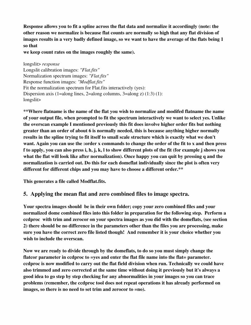
Response allows you to fit a spline across the flat data and normalize it accordingly (note: the other reason we normalize is because flat counts are normally so high that any flat division of images results in a very badly defined image, so we want to have the average of the flats being 1 so thatwe keep count rates on the images roughly the same).

longslit> responseLongslit calibration images: "Flat.fits"Normalization spectrum images: "Flat.fits"Response function images: "Modflat.fits"Fit the normalization spectrum for Flat.fits interactively (yes): Dispersion axis (1=along lines, 2=along columns, 3=along z) (1:3) (1): longslit> 

**Where flatname is the name of the flat you wish to normalize and modifed flatname the name of your output file, when prompted to fit the spectrum interactively we want to select yes. Unlike the overscan example I mentioned previously this fit does involve higher order fits but nothing greater than an order of about 6 is normally needed, this is because anything higher normally results in the spline trying to fit itself to small scale structure which is exactly what we don't want. Again you can use the :order x commands to change the order of the fit to x and then press f to apply, you can also press i, h, j, k, l to show different plots of the fit (for example j shows you what the flat will look like after normalization). Once happy you can quit by pressing q and the normalization is carried out. Do this for each domeflat individually since the plot is often very different for different chips and you may have to choose a different order.**

This generates a file called Modflat.fits.

5.  Applying the mean flat and zero combined files to image spectra.

Your spectra images should  be in their own folder; copy your zero combined files and your normalized dome combined files into this folder in preparation for the following step.  Perform a ccdproc  with trim and zerocor on your spectra images as you did with the domeflats, (see section2) there should be no difference in the parameters other than the files you are processing, make sure you have the correct zero file listed though!  And remember it is your choice whether you wish to include the overscan.

Now we are ready to divide through by the domeflats, to do so you must simply change the flatcor parameter in ccdproc to =yes and enter the flat file name into the flat= parameter. ccdproc is now modified to carry out the flat field division when run. Technically we could have also trimmed and zero corrected at the same time without doing it previously but it's always a good idea to go step by step checking for any abnormalities in your images so you can trace problems (remember, the ccdproc tool does not repeat operations it has already performed on images, so there is no need to set trim and zerocor to =no).

longslit> epar ccdproc  I R A F                      Image Reduction and Analysis FacilityPACKAGE = ccdred   TASK = ccdproc

images  =         @listobj.dat  List of CCD images to correct(output =                     ) List of output CCD images(ccdtype=                     ) CCD image type to correct(max_cac=                    0) Maximum image caching memory (in Mbytes)(noproc =                   no) List processing steps only?

(fixpix =                   no) Fix bad CCD lines and columns?(oversca=                   no) Apply overscan strip correction?(trim   =                  yes) Trim the image?(zerocor=                  yes) Apply zero level correction?(darkcor=                   no) Apply dark count correction?(flatcor=                  yes) Apply flat field correction?(illumco=                   no) Apply illumination correction?(fringec=                   no) Apply fringe correction?(readcor=                   no) Convert zero level image to readout correction?(scancor=                   no) Convert flat field image to scan correction?

(readaxi=                 line) Read out axis (column|line)(fixfile=                     ) File describing the bad lines and columns(biassec=   [2048:2112,5:1000]) Overscan strip image section(trimsec=    [150:2047,5:1000]) Trim data section(zero   =                 Zero) Zero level calibration image(dark   =                     ) Dark count calibration image(flat   =         Modflat) Flat field images(illum  =                     ) Illumination correction images(fringe =                     ) Fringe correction images(minrepl=                   1.) Minimum flat field value(scantyp=            shortscan) Scan type (shortscan|longscan)(nscan  =                    1) Number of short scan lines

(interac=                   no) Fit overscan interactively?(functio=            chebyshev) Fitting function(order  =                    1) Number of polynomial terms or spline pieces(sample =                    *) Sample points to fit(naverag=                    1) Number of sample points to combine(niterat=                    1) Number of rejection iterations(low_rej=                   3.) Low sigma rejection factor(high_re=                   3.) High sigma rejection factor(grow   =                   0.) Rejection growing radius(mode   =                   ql)

longslit> ccdprocList of CCD images to correct (@listobj.dat): longslit>

the resulting images should be ready for spectral extraction but you should get someone familiar with iraf and spectra to check your work. Several problems can also arise at this point:

Your flats may have areas of zero or negative amplitude, if this is the case then when dividing through by your flats during the final ccdproc run you will receive an error akin toERROR! floating point attempt to divide by zero!The only way i have found to fix this is using the imreplace tool under images>imutil>imreplaceThis tool allows you to specify a value which replaces and pixels with current  values between a range (use >help imreplace while in imutil for a rundown of it's parameters). The value with which you replace the pixels is of course tricky to choose, going very low is almost as bad as having zero points since the division will result in very high values at your low regions which causes flattening of the rest of your image. One option is to match a value closest to other low areas on your image, for example mine included a dark line of 0 value, which i replaced with the rough value of other dark lines on the image which hovered around 0.04, thus i chose 0.01, lower than the others but not of an order that differed too greatly.

6. Selecting object and sky regions.

Get a hold of a copy of "A user's guide to reducing slit spectra with IRAF" by Phil Massey, Frank Valdes and Jeanette Barnes and read through the first few chapters, I will make references to it as we go along, but the earlier parts will give you some idea of what I'm referring to if you have had no  previous experience.

a.   Identifying your source.  I find it easiest to use ds9 for this.  If your images are anything like mine you will see a number of horizontal and vertical lines running across your image, dependingon the orientation of your CCD these lines are night sky lines (the background lines due to background light) and spectra from stars in the slit. The lines that start and end abruptly at the top and bottom of the images are likely the sky lines, those that fade off at one end of the images (normally due to the filter being more sensitive at one end of the spectrum) are likely object spectra. Knowing where your target was at the time of image capture can help you identify whichof the lines corresponds to it.  If you don't know the target hopefully you know something about it (a prominent line) in order to identify it!  Once you know the location of your source and decided on the size of your source extraction region and background extraction region you can use kpnoslit to extract a spectrum.

b.   Extracting a spectrum from a line on your image.  You will be using the apall tool under the following commands:

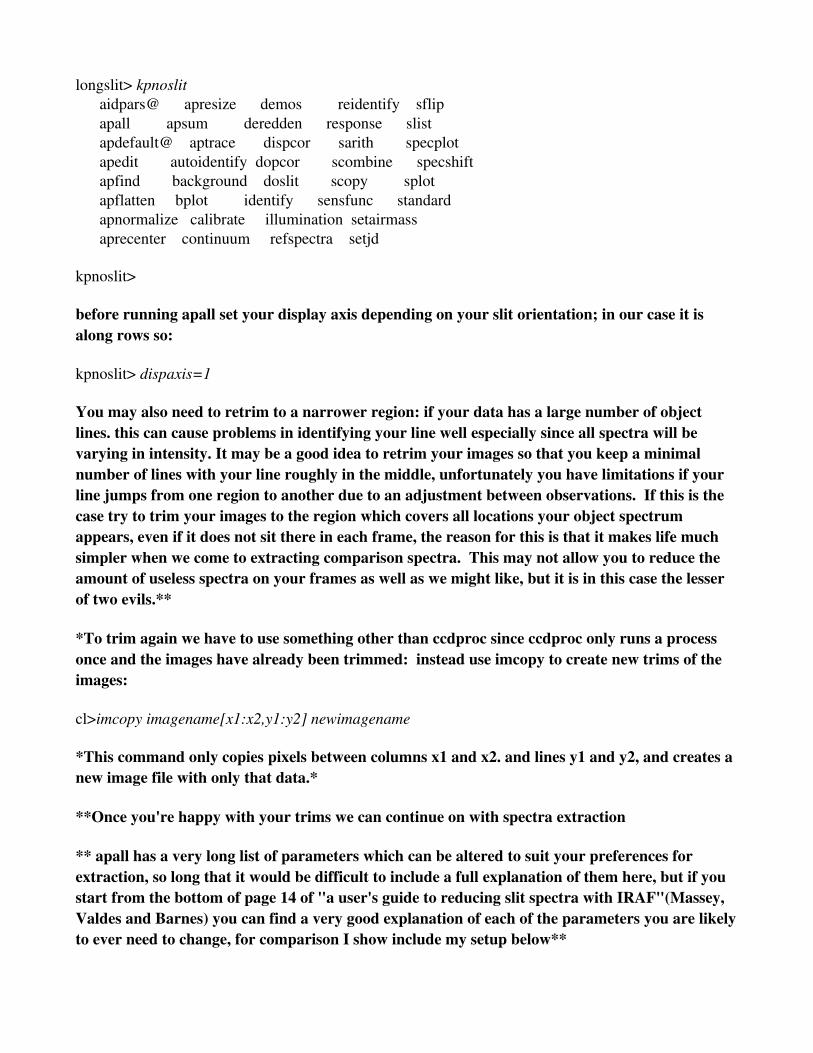
longslit> kpnoslit      aidpars@      apresize      demos         reidentify    sflip      apall         apsum         deredden      response      slist      apdefault@    aptrace       dispcor       sarith        specplot      apedit        autoidentify  dopcor        scombine      specshift      apfind        background    doslit        scopy         splot      apflatten     bplot         identify      sensfunc      standard      apnormalize   calibrate     illumination  setairmass          aprecenter    continuum     refspectra    setjd         

kpnoslit> 

before running apall set your display axis depending on your slit orientation; in our case it is along rows so:

kpnoslit> dispaxis=1

You may also need to retrim to a narrower region: if your data has a large number of object lines. this can cause problems in identifying your line well especially since all spectra will be varying in intensity. It may be a good idea to retrim your images so that you keep a minimal number of lines with your line roughly in the middle, unfortunately you have limitations if your line jumps from one region to another due to an adjustment between observations.  If this is the case try to trim your images to the region which covers all locations your object spectrum appears, even if it does not sit there in each frame, the reason for this is that it makes life much simpler when we come to extracting comparison spectra.  This may not allow you to reduce the amount of useless spectra on your frames as well as we might like, but it is in this case the lesser of two evils.**

*To trim again we have to use something other than ccdproc since ccdproc only runs a process once and the images have already been trimmed:  instead use imcopy to create new trims of the images:

cl>imcopy imagename[x1:x2,y1:y2] newimagename

*This command only copies pixels between columns x1 and x2. and lines y1 and y2, and creates a new image file with only that data.*

**Once you're happy with your trims we can continue on with spectra extraction

** apall has a very long list of parameters which can be altered to suit your preferences for extraction, so long that it would be difficult to include a full explanation of them here, but if you start from the bottom of page 14 of "a user's guide to reducing slit spectra with IRAF"(Massey, Valdes and Barnes) you can find a very good explanation of each of the parameters you are likelyto ever need to change, for comparison I show include my setup below**

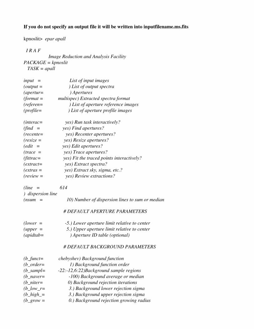
If you do not specify an output file it will be written into inputfilename.ms.fits

kpnoslit>  epar apall

  I R A F                      Image Reduction and Analysis FacilityPACKAGE = kpnoslit   TASK = apall    input   =                       List of input images(output =                     ) List of output spectra(apertur=                     ) Apertures(format =            multispec) Extracted spectra format(referen=                     ) List of aperture reference images(profile=                     ) List of aperture profile images

(interac=                  yes) Run task interactively?(find   =                  yes) Find apertures?(recente=                  yes) Recenter apertures?(resize =                  yes) Resize apertures?(edit   =                  yes) Edit apertures?(trace  =                  yes) Trace apertures?(fittrac=                  yes) Fit the traced points interactively?(extract=                  yes) Extract spectra?(extras =                  yes) Extract sky, sigma, etc.?(review =                  yes) Review extractions?

(line   =                614)  dispersion line(nsum   =                   10) Number of dispersion lines to sum or median

                                # DEFAULT APERTURE PARAMETERS

(lower  =                  ­5.) Lower aperture limit relative to center(upper  =                   5.) Upper aperture limit relative to center(apidtab=                     ) Aperture ID table (optional)

                                # DEFAULT BACKGROUND PARAMETERS

(b_funct=            chebyshev) Background function(b_order=                    1) Background function order(b_sampl=          ­22:­12,6:22)Background sample regions(b_naver=                   ­100) Background average or median(b_niter=                    0) Background rejection iterations(b_low_r=                   3.) Background lower rejection sigma(b_high_=                   3.) Background upper rejection sigma(b_grow =                   0.) Background rejection growing radius

                                # APERTURE CENTERING PARAMETERS

(width  =                   5.) Profile centering width(radius =                  10.) Profile centering radius(thresho=                   0.) Detection threshold for profile centering

                                # AUTOMATIC FINDING AND ORDERING PARAMETERS

nfind   =                    0)number of apertures to be found automatically(minsep =                   5.) Minimum separation between spectra(maxsep =                1000.) Maximum separation between spectra(order  =           increasing) Order of apertures

                                # RECENTERING PARAMETERS

(aprecen=                     ) Apertures for recentering calculation(npeaks =                INDEF) Select brightest peaks(shift  =                  yes) Use average shift instead of recentering?

                                # RESIZING PARAMETERS

(llimit =                INDEF) Lower aperture limit relative to center(ulimit =                INDEF) Upper aperture limit relative to center(ylevel =                  0.1) Fraction of peak or intensity for automatic widt(peak   =                  yes) Is ylevel a fraction of the peak?(bkg    =                  yes) Subtract background in automatic width?(r_grow =                   0.) Grow limits by this factor(avglimi=                   no) Average limits over all apertures?

                                # TRACING PARAMETERS

(t_nsum =                   10) Number of dispersion lines to sum(t_step =                   10) Tracing step(t_nlost=                    3) Number of consecutive times profile is lost befo(t_funct=             legendre) Trace fitting function(t_order=                    2) Trace fitting function order(t_sampl=                    *) Trace sample regions(t_naver=                    1) Trace average or median(t_niter=                    0) Trace rejection iterations(t_low_r=                   3.) Trace lower rejection sigma(t_high_=                   3.) Trace upper rejection sigma(t_grow =                   0.) Trace rejection growing radius

                                # EXTRACTION PARAMETERS

(backgro=                  fit) Background to subtract

(skybox =                    1) Box car smoothing length for sky(weights=             variance) Extraction weights (none|variance)(pfit   =                fit1d) Profile fitting type (fit1d|fit2d)(clean  =                   no) Detect and replace bad pixels?(saturat=                INDEF) Saturation level(readnoi=                 4.50) Read out noise sigma (photons)(gain   =                  0.7) Photon gain (photons/data number)(lsigma =                   4.) Lower rejection threshold(usigma =                   4.) Upper rejection threshold(nsubaps=                    1) Number of subapertures per aperture(mode   =                   ql)

**The most important points about apall come when we enter the interactive mode, when you run apall on a particular image

kpnoslit>apall [imagename]

This will bring up a plot of a cut along the spatial axis. The peaks you should see are the object lines that run down the dispersion axis, what we are about to do requires we know which of thesepeaks is our source. What we are about to do (in a nutshell) is tell IRAF (via apall) which line is our source, where the background spectra that we want to remove from it is, and what path or "trace" to follow across the image which the line marks across it.

Apall will select the brightest feature automatically and deem it "aperture 1", this may not be our source so we can delete it using the interactive command d, we can then mark the correct peak by  placing the cursor over it and pressing m, this should mark the peak as "aperture 1". Apall will select default positions (defined in the parameters) for the background, these may not be the best place for them and can vary from image to image so we are going to take a look at them manually.   Clicking m in plot will center on aperture location.  Clicking r will refresh and display background regions (identified in parameter file relative to the source location).  We can take a closer look at our selected peak and the designated background regions by pressing b, the background regions are marked along the bottom (one either side of the peak). When selecting these regions we wish to avoid them overlapping with the "wings" of the peak, or any other peaks nearby, i.e. it is preferable that they encompass relatively flat regions either side of our peak. to remove any current regions press t (note that they do not vanish from your display, press f to update the "fit" as in previous interactive processes), you may now mark new regions by pressing s at the start of a new region, and again where you wish it to end, you can create as many of these regions as you like, but try to keep them down to 2 relatively wide spots, one eitherside, unless your region is particularly noisy, in which case you may create multiuple smaller selections.  When you are happy with your background selections press f, and then q to quit backto the starting plot.

You can now press q again, you will be given several prompts, select yes to them all, the last will be similar to "do you wish to alter the trace interactively", when you say yes to this you will be 

taken to a plot of the locations of the lines strongest regions as we move down the chip, our goal isto provide a fitting function that best follows these points so that the program can accurately follow the line across the image. Like our previous line fitting exercises (domeflat normalization) we wish to get a close fit to the line without using too high an order (ideally no more than 5 in thiscase) you can do so just as before using :order # and then hitting the f key. Also if your data happens to have any odd anomalies (such as a cosmic ray near the line) which causes a point to deviate from the norm you can delete it using d while the cursor is near it on the screen, or returnit using u, you may then refit the function with f to give you a closer relationship to the rest of thepoints.

Once you are happy with the fit, hit q once more, and say yes to the rest of the prompts (note thatthese prompts and the previous ones include the option of saving your markings and backgroundselections so everything should remain the same if you were to run apall again). The display will provide you with the extracted spectrum.  Hit q in command window to return to the console.

Now all you need to do is run apall for all your images and run through the checks and amendments above accordingly, take note that the line may not be in the same location in every image if an adjustment to the telescope was made between observations, but object spectra positions relative to each other should allow you to track down your source from image to image.

7.   Cleaning  your spectra.

Depending on your data and what you want from the resulting spectra you can now use the wonderful tool splot to make amendments to your extracted spectra. It is found under the same listing as apall so you should not have to go anywhere after having performed your extractions.

splot allows you to view and alter spectra in a variety of ways, you can find a detailed list of commands using a kp>help splot command, but if your spectra are similar to mine the following commands should suffice.

First of all we have to deal with any nasty anomalies that may have intruded upon out spectra. When doing so it would be best to have the images you took the lines from loaded up on Ds9 where you can look at the line itself in more detail.

These anomalies can come from various sources but the most common i've found are the following.

Cosmic rays: You are sure to have noticed these bright streaks and spots on your CCD images, more often than not they can be ignored as they have no impact on your data, but every now and then they can impact upon your line or near it which can interfere in various ways. If one 

happens to cross your spectral line you will see a large very narrow peak in your spectra when looking at it via splot, alternatively if the ray happens to cross your background region you should find a narrow large dip in your spectrum (since the extraction process will have subtracted the large ray amplitude from your spectrum as part of the background). More complicated occurrences can involve a cosmic ray streaking diagonally across your line where it interferes with the spectra directly and the background either side of the line, resulting in a dip, peak, dip pattern.  Such anomalies should remain sharp, in which case the following tricks should allow you to remove them without much ill effect (though if they occur in a particularly sensitive area on your spectrum they pose a much greater problem).  Where you have to be careful is if a ray happens to streak close to the horizontal in any of your data regions, when this occurs, errors are not simply sharp peaks, but can cause regions in your spectrum of abnormally high or low values.

CCD errors: Though we may have accounted for some errors when we subtracted the domeflat from our images, some pixel faults can still arise, this requires detailed examination of your images through a display program while editing them. Should you see a sharp dip that doesn't correspond to a cosmic ray error and yet also doesn't resemble a spectrum feature, take a close look at the region in your viewer, you may see that a small line of pixels in the spatial direction appear darker (if they stretch beyond the width of your objects spectral line and yet are not part of a skyline), or even a line that streaks along entire columns and yet is too sharply defined to be a sky line. Such errors normally repeat themselves across a range of images, and so appear in thesame place in your spectra, thus care must be taken to not confuse them with true spectral features, normally they give themselves away by being only one or two pixels wide and far lower in magnitude than the rest of the line, but if you are unsure a second opinion is always a good idea.

In all cases you will have to take into account the position of your anomalies, for example anomalies that occur in emission peaks of absorption regions that are important to your analysis typically render that frame useless, since it is very difficult to remove the problem without compromising your data. A lot of the time though all they do is make your spectrum look messy, large values can cause the rest of your spectrum to look flat and so should be removed to allow the rest of the detail to be obvious.

So now that we know what features are true anomalies how can we remove them? This is where splot really works, you can zoom in on a region by hitting a with your cursor in one corner of the region, and then again with it in the opposite corner. Once zoomed in on your anomaly region wecan use the j button to "fudge" the value of pixels at the x value of your cursor to its y value, thusyou can manually average large spikes to a value close to neighboring pixels.  You can then zoom out using c, and save the image to a new file by using i, and typing a new name, quit via q as usual. While this may seem a very hasty way of cleaning up the spectra, as long as you only care about specific regions in the data which are unaffected, you can get away with it, sharp spikes vanish easily without leaving any noticeable sign, and large regions of error can be simply flattened out (though you can still see where such an error was it will allow you to view the rest of

the spectrum in detail).

Of course this means you must view and edit each spectrum individually, which takes up a lot of time, but it allows you to check for anything unusual in your data in the mean time, which never hurts.

There is one further function in splot worth mentioning at this point and that is the smoothing function, if you hit s you will be asked for a pixel width over which each point in the spectrum will be averaged (at least that is how I understand it). Like the value fudging this ability may alsocompromise your data, on the other hand it can provide a quick and easy way of tidying up aspectrum if only for presentation purposes. you can repeat the smoothing with the same value multiple times for a cumulative effect, just be sure to remember that the changes are only implemented once you save to a file by using i as before.

8. Calibration:  a)  Extracting comparison spectra.

So now we have our cleaned spectra, we need to know what exactly we're looking at, this is whereARCS taken with your spectra come in. What we require from the arcs is a trace matching that of each spectra, only applied to the arcs themselves, this will provide us with a comparison known spectrum at the exact same position that our object spectra lied. We can then identify peaks on the comparison spectrum, map a wavelength scale on to them, and use them as a reference to gives us a wavelength scale for our extracted object spectra.  The hard part is deciding which arcs will go with which spectra, ideally we'd like to have arcs taken very close to the time the spectra frames were taken, but this is not always possible as it can be time costly. Mydata included arcs taken every dozen frames or so. Now if you were lucky, your object spectra lines remained in roughly the same region so your cuts should all be the same, in which case we can simply extract comparison spectra from arcs either side of each image (i.e. the one before andone after) and both can be used later on.   Unfortunately if you couldn't avoid it (or just didn't realize at the time that it may cause problems later ­ me) and your cuts are the same size but simply vary in location across your images, then you will have to make the same size cuts for eacharc which was taken nearest in time to each spectrum, and then proceed with extracting a comparison spectrum... I'm going to hope you didn't do this, because it does make life much harder for you.

Copy over your arc files and trim them to match the images from which you extracted your object spectra using the ccdproc parameters for your source images.  Also trim them using imcopy as for the object file.

The basic command we will now use is simply apall with a few amendments:**

kp>apall comparisonimage out=comparisonspectra ref=objectimage recen­ trace­ back­ intera­

*"comparisonimage" is the arc trim related to the spectra you extracted from the "objectimage" trim and the output file name will be whatever you input instead of "comparisonspectra", the reference file is the original object file (as trimmed with imcopy).  The extra commands at the end will cause apall to use the aperture and trace details from the original image and disable the interactive interface so we get the new comparison spectrum along the exact same trace.

You can either do this for a single arc taken nearest to each spectra, or two nearest either side as mentioned (though this will be more accurate, it will be trickier).

Of course this is going to get quite boring if we have to do this for each image at a time, it is easier to use lists (hopefully you know how to do this from use of linux, if not a basic rundown isls (images you want in the list) > images.lisYou can then copy this list and modify it to create a list of output images using vi, you also have to create a corresponding arc trim list. The result should be 3 lists of the same number of lines which alters the command to extract spectra to:

kpnoslit> apall @comparisonimages.lis out=@comparisonspectra.lis ref=@objectimages.lis recen­ trace­ back­ intera­

You should now have one or two comparison spectra per object spectrum, now we must map a wavelength scale on to the comparison spectra by determining their dispersion solutions.

    8b) Calibration:  determining the comparison spectra dispersion solutions

We will be using the tools identify and reidentify for this, both found under kpnoslit, but we will also need a spectrum atlas to allow us to identify peaks.  There should be some available at telescope websites, normally one for each piece of equipment and filter. The identifying parameters should be:

kpnoslit> epar identify

                    Image Reduction and Analysis FacilityPACKAGE = kpnoslit   TASK = identify

images  =                       Images containing features to be identified(section=          middle line) Section to apply to two dimensional images(databas=             database) Database in which to record feature data(coordli= linelists$idhenear.dat) User coordinate list(units  =                     ) Coordinate units(nsum   =                   10) Number of lines/columns/bands to sum in 2D image(match  =                  ­3.) Coordinate list matching limit(maxfeat=                   50) Maximum number of features for automatic identif(zwidth =                 100.) Zoom graph width in user units

(ftype  =             emission) Feature type(fwidth =                   8.) Feature width in pixels(cradius=                   5.) Centering radius in pixels(thresho=                   0.) Feature threshold for centering(minsep =                   2.) Minimum pixel separation(functio=              spline3) Coordinate function(order  =                    1) Order of coordinate function(sample =                    *) Coordinate sample regions(niterat=                    0) Rejection iterations(low_rej=                   3.) Lower rejection sigma(high_re=                   3.) Upper rejection sigma(grow   =                   0.) Rejection growing radius(autowri=                   no) Automatically write to database(graphic=             stdgraph) Graphics output device(cursor =                     ) Graphics cursor inputcrval   =                       Approximate coordinate (at reference pixel)cdelt   =                       Approximate dispersion(aidpars=                     ) Automatic identification algorithm parameters(mode   =                   ql)

The important one to note is the coordli, this is the wavelength reference file to which the identifyprogram will be trying to match your spectrum, there is a list of other available line lists under:

page linelists$README

under which another file may be more suited to your arc spectra. The otherparameter to take note of is fwidth, if your arc spectral lines happen to be noticeably wider or narrower you may wish to alter this value to reflect that, it is the base to base width of your "spectral features".

When you run this task on a comparison spectrum file:

kpnoslit> identify comparisonspectrum.fits

You are given a plot of the comparison spectrum, to get a dispersion solution we must now identify a few good lines and proceed from there...

The following is going to be similar to the process we went through to mark and find the trace forour object spectrum, the plot will at first be unmarked but you can mark a peak on the line usingm and then entering the corresponding wavelength value for the line that you find on the atlas (note it doesn't have to be perfect, the linelist will find a feature close to the value you entered butit doesn't hurt to try to be accurate from the start). Once you've marked 2 or 3 good lines hit f to see the fit of your lines to the information stored in the line list. You will see a display very much like the fitting display used to fit the trace during our extraction and it works in much the same way, enter the order for your fit using :order # and f, and view the changes using h, j, k  and l. 

Try an order 2 fit and then return to the original plot by pressing q, we can now try hitting l to mark other possible lines on the plot that correspond to a fit with the original marked lines. Hit f again to view the new distribution of points alongside the fit.

When viewing the residuals you may notice some of the points deviating greatly from the fit, suchpoints are likely to be mismarked lines and should be deleted using d as we did in the spectral extraction process,  BUT! it is also possible the other points are in fact the ones that have been incorrectly marked and the function fitting to them is what is making the other lines appear incorrect, it is a good idea to switch between the fitting display and the original plot to see if any of the marks do not lie on a peak at all, or in a region with a lot of noise where one peak can be easily confused for an actual feature as these are the most likely to be at fault. Decisions like this involve a careful eye and some logic, but what we are aiming to do do is reduce the rms value in the top right corner of the residuals plot down to something below 0.01 or so, any higher and we are risking a bad fit. If at some point you delete a line you did not want to, hit l and start again from the full list of lines, also try deleting the erroneous lines in different orders and refitting each time as you may find that deleting one erroneous line can completely change the plot and make other erroneous lines suddenly fit. As always try not to increase the order of your fit above a certain value, in this case I would say 4 is as high as you should go, and very often 2 is enough and you should aim to delete more lines rather than increase order to obtain a better fit unless the lines are very well exposed.

Once you are happy with your fit hit q, the information is now saved and we can use the images fit to aid us with the rest using the reidentify tool.  Reidentify can be can be run on all other arcs cut along similar locations in order to try to match our new fit from one on to the others, very often this is quite accurate and the rms should remain low, but if it does deviate we can again go into the offending spectrum and amend it's own personal fit for better accuracy (i.e.  lowering it'srms value).  To do so simply say yes when asked if you would like to alter the fit interactively for each erroneous spectrum.

8c)  Calibration: Assigning dispersion solutions to object spectra

Now we have to assign each object spectrum it's corresponding comparison spectra, there are several methods, depending on how many comparison spectra you have so we'll tackle each method individually. The basic thing you need to know is that we are going to add a new parameter to the headers of all the object spectra .ms.fits files, where the name of the corresponding comparison spectra images are to be located.

One comparison per spectra:  we need only add one extra parameter to our headers here, so the first step is to add the blank parameter label to all our spectra, the label being REFSPEC1

To add the line we must modify hedits parameters:kpnoslit>  epar heditPACKAGE = imutil   TASK = hedit

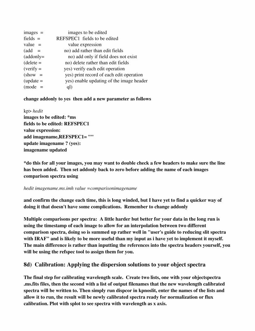
images  =  images to be editedfields  =             REFSPEC1  fields to be editedvalue   =  value expression(add    =                   no) add rather than edit fields(addonly=                   no) add only if field does not exist(delete =                   no) delete rather than edit fields(verify =                  yes) verify each edit operation(show   =                  yes) print record of each edit operation(update =                  yes) enable updating of the image header(mode   =                   ql)

change addonly to yes  then add a new parameter as follows

kp> heditimages to be edited: *msfields to be edited: REFSPEC1value expression:add imagename,REFSPEC1= ""update imagename ? (yes):imagename updated

*do this for all your images, you may want to double check a few headers to make sure the line has been added.  Then set addonly back to zero before adding the name of each images comparison spectra using

hedit imagename.ms.imh value =comparisonimagename

and confirm the change each time, this is long winded, but I have yet to find a quicker way of doing it that doesn't have some complications.  Remember to change addonly

Multiple comparisons per spectra:  A little harder but better for your data in the long run is using the timestamp of each image to allow for an interpolation between two different comparison spectra, doing so is summed up rather well in "user's guide to reducing slit spectra with IRAF" and is likely to be more useful than my input as i have yet to implement it myself. The main difference is rather than inputting the references into the spectra headers yourself, youwill be using the refspec tool to assign them for you.

8d)  Calibration: Applying the dispersion solutions to your object spectra

The final step for calibrating wavelength scale.  Create two lists, one with your objectspectra .ms.fits files, then the second with a list of output filenames that the new wavelength calibrated spectra will be written to. Then simply run dispcor in kpnoslit, enter the names of the lists and allow it to run, the result will be newly calibrated spectra ready for normalization or flux calibration. Plot with splot to see spectra with wavelength as x axis.

Onedspec> epar dispcor I R A F Image Reduction and Analysis FacilityPACKAGE = onedspec TASK = dispcor

input = List of input spectraoutput = List of output spectra(lineari= yes) Linearize (interpolate) spectra?(databas= database) Dispersion solution database(table = ) Wavelength table for apertures(w1 = INDEF) Starting wavelength(w2 = INDEF) Ending wavelength(dw = INDEF) Wavelength interval per pixel(nw = INDEF) Number of output pixels(log = no) Logarithmic wavelength scale?(flux = yes) Conserve total flux?(blank = 0.) Output value of points not in input(samedis= no) Same dispersion in all apertures?(global = no) Apply global defaults?(ignorea= no) Ignore apertures?(confirm= no) Confirm dispersion coordinates?(listonl= no) List the dispersion coordinates only?(verbose= yes) Print linear dispersion assignments?(logfile= ) Log file(mode = ql)

9. Writing spectral files in ascii for input to molly and Doppler.First convert spectra to one d(imension) using scopy within onedspec.  Onedspec> epar scopy          I R A F                      Image Reduction and Analysis FacilityPACKAGE = onedspec   TASK = scopyinput   =                       List of input spectraoutput  =                       List of output spectra(w1     =                INDEF) Starting wavelength(w2     =                INDEF) Ending wavelength(apertur=                     ) List of input apertures or columns/lines(bands  =                     ) List of input bands or lines/bands(beams  =                     ) List of beams or echelle orders(apmodul=                    0) Input aperture modulus (0=none)(format =            multispec) Output spectra format(renumbe=                   no) Renumber output apertures?(offset =                    0) Output aperture number offset

(clobber=                   no) Modify existing output images?(merge  =                   no) Merge with existing output images?(rebin  =                  yes) Rebin to exact wavelength region?(verbose=                   no) Print operations?(mode   =                   ql)

You can check your one d spectra using splot.  Then use wspectext to write out in ascii (set the parameter header to no if you want to use this for molly).onedspec> epar wspectext                     I R A F                      Image Reduction and Analysis FacilityPACKAGE = onedspec   TASK = wspectextinput   =  GuMus2057.0001.fits  Input list of image spectraoutput  =         GuMus2057txt  Output list of text spectra(header =                   no) Include header?(wformat=                     ) Wavelength format(mode   =                   ql)