steric sea level changes estimated from historical ocean

155

Journal of Oceanography, Vol. 62, pp. 155 to 170, 2006

Keywords:⋅⋅⋅⋅⋅ Temperatureanalysis,

⋅⋅⋅⋅⋅ salinity analysis,⋅⋅⋅⋅⋅ steric sea level,⋅⋅⋅⋅⋅ TOPEX/Poseidon,⋅⋅⋅⋅⋅ tide gauge,⋅⋅⋅⋅⋅ crustal movement.

* Corresponding author. E-mail: [email protected] leave from the Meteorological Research Institute of the Japan

Meteorological Agency.

Copyright © The Oceanographic Society of Japan.

Steric Sea Level Changes Estimated from HistoricalOcean Subsurface Temperature and Salinity Analyses

MASAYOSHI ISHII1*, MASAHIDE KIMOTO2, KENJI SAKAMOTO3 and SIN-ITI IWASAKI4

1Frontier Research Center for Global Change, Japan Agency for Marine-Earth Science and Technology, Yokohama 236-0001, Japan2Center for Climate System Research, University of Tokyo, Kashiwa 277-8586, Japan3Climate Prediction Division, Japan Meteorological Agency, Tokyo 100-8122, Japan4National Research Institute for Earth Science and Disaster Prevention, Tsukuba 305-0006, Japan

(Received 29 August 2005; in revised form 12 November 2005; accepted 28 November 2005)

An historical objective analysis of subsurface temperature and salinity was carriedout on a monthly basis from 1945 to 2003 using the latest observational databasesand a sea surface temperature analysis. In addition, steric sea level changes weremainly examined using outputs of the objective analyses. The objective analysis is arevised version of Ishii et al. and is available at 16 levels in the upper 700 m depth.Artificial errors in the previous analysis during the 1990s have been worked out inthe present analysis. The steric sea level computed from the temperature analysis hasbeen verified with tide gauge observations and TOPEX/Poseidon sea surface heightdata. A correction for crustal movement is applied for tide gauge data along the Japa-nese coast. The new analysis is suitable for the discussion of global warming. Valida-tion against the tide gauge reveals that the amplitude of thermosteric sea level be-comes larger and the agreement improves in comparison with the previous analysis.A substantial part of local sea level rise along the Japanese coast appears to be ex-plained by the thermosteric effect. The thermal expansion averaged in all longitudesfrom 60°S to 60°N explains at most half of recent sea level rise detected by satelliteobservation during the last decade. Considerable uncertainties remain in steric sealevel, particularly over the southern oceans. Temperature changes within MLD makeno effective contribution to steric sea level changes along the Antarctic CircumpolarCurrent. According to statistics using only reliable profiles of the temperature andsalinity analyses, salinity variations are intrinsically important to steric sea levelchanges in high latitudes and in the Atlantic Ocean. Although data sparseness is se-vere even in the latest decade, linear trends of global mean thermosteric and halostericsea level for 1955 to 2003 are estimated to be 0.31 ± 0.07 mm/yr and 0.04 ± 0.01mm/yr, respectively. These estimates are comparable to those of the former studies.

(2005b; LAB05, hereafter) reported that the temperatureof the global oceans in the upper 3000 m depths has in-creased by 0.037°C during the period between 1955 and1998. After the publication of the Third Assessment Re-port by the Intergovernmental Panel on Climate Changein 2001 (IPCC TAR), global mean sea level rise (SLR)has been studied intensively in collaboration with vari-ous communities relevant to geophysics and astronomy(Cazenave and Nerem, 2004). Recently, Antonov et al.(2005) estimated a trend of global mean thermosteric sealevel, due to thermal expansion, of 0.33 mm/yr using thetemperature analysis of LAB05. This estimate is about 5times smaller than 1.84 mm/yr computed from tide gauge

1. IntroductionThe roles of oceans as a huge reservoir of heat and

water are important in the global climate system. Globalwarming is now proceeding, and therefore it becomesincreasingly important to understand what happened inthe global oceans during the last century. Recent studiessuggest warming of the world oceans; Levitus et al.

156 M. Ishii et al.

data (Douglas and Peltier, 2002), although the tide gaugeobservations are poorly distributed in space and the datasuffer from crustal movement at the stations (Cazenaveand Nerem, 2004). In contrast, the estimate of global sealevel trend from tide gauge data is not significantly dif-ferent when an isostatic adjustment is taken into account(Peltier, 2001). For the period from 1993 to 2003, recentstudies show that thermosteric sea level rise is around1.2–1.5 mm/yr (Willis et al., 2004; Antonov et al., 2005),while an analysis of the TOPEX/Poseidon sea surfaceheight (Chambers et al., 2003) shows a doubled trend of2.8 mm/yr for the same period (Cazenave and Nerem,2004). To explain the smaller trends of thermosteric sealevel than those of the direct sea level measurement,Antonov et al. (2002) suggested that input of fresh waterto the oceans explains the remainder of sea level rise onthe basis of evidence of salinity freshening in their salin-ity analysis. However, large uncertainty remained in theestimation of SLR (Church et al., 2001) since the watercirculation between climate subsystems of atmosphere,ocean, and land surface is quantitatively unknown. Thecharacteristics of thermosteric sea level variations ondecadal time scales over the global oceans are examinedby Lombard et al. (2005) comparing two historical tem-perature analyses by Levitus et al. (2000) and Ishii et al.(2003; IKK03, hereafter). In particular, the thermostericsea levels vary in phase with dominant modes of climatevariability such as El Niño and the Southern Oscillation,Pacific Decadal Oscillation (PDO), and North AtlanticOscillation. Stephens et al. (2001) also reported that Pa-cific Ocean heat content changes in phase with PDO.

The present study follows IKK03 in which a histori-cal objective analysis of oceanic temperature was carriedout on a monthly basis for the period from 1950 to 1998.A major purpose is to make an objective analysis of tem-perature and salinity for use in climate studies. The pre-vious analysis scheme is improved for better representa-tion of climate variations, and the new objective analysisis applied to examine historical sea level changes. Errorsin steric sea level are also estimated. One concern of thisinvestigation is how the geographic distribution of cli-mate anomalies is reproduced whereas only the spatio-temporal averages are discussed in the pioneering re-searches mentioned above. In addition, local changes insea level are of great concern here as this is one of seri-ous problems under global warming for human beings.Oceanographical observations suffer from noise and lackof representativeness due to the existence of meso-scaleeddies. These affect the ocean analyses and interpretingsuch an analysis may not be easy. The analysis schemeused in this study is based on a recent methodology ofobjective analysis (Derber and Rosati, 1989; Ghil andMalanotte-Rizzoli, 1991), and is superior in reducingobservational noise in a resultant analysis as described in

IKK03 and Section 2. Similar objective analysis schemesbased on optimal interpolation have been applied to SSTanalyses (Reynolds and Smith, 1994; Ishii et al., 2005),and are successful in reducing the observational noise inSST data.

The objective analysis of monthly ocean subsurfacetemperature by IKK03 has several deficiencies, mainlydue to the mixture of observational databases of subsur-face temperature and sea surface temperature (SST). Al-though the analysis shows good agreement with Levituset al., 2000) according to the above-mentioned compari-son study, a large discrepancy appears in global meanthermosteric sea level in the 1990s. In year 1991, an ob-servational data set, the World Ocean Data 1994 edition(WOD94), was replaced by an operational database col-lected by the global telecommunication system (GTS) andJapanese domestic communication lines. Regarding thelatter database, an expendable bathythermograph (XBT)drop rate correction proposed by Hanawa et al. (1995)was not applied to the data because the data set does notstore the XBT probe type. An objective analysis withoutthis correction results in a significantly low thermostericsea level. There is another minor discontinuity in theanalysis due to replacement of SST analysis in 1995,which is used to determine mixed layer temperature inthe objective analysis.

The present study uses the latest observational dataset and an SST analysis: the World Ocean Data 2001 edi-tion (WOD01; Boyer et al., 2001) and COBE SST (COBE:Centennial in-situ Observation Based Estimates of vari-ability of SST and marine meteorological variables; Ishiiet al., 2005). New monthly temperature and salinity analy-ses are described in Section 2, as well as changes in qual-ity control and objective analysis schemes. Section 3presents the analysis results, verifying them against sat-ellite and tidal sea level observations. In addition,halosteric sea level variation, that is sea level variationdue to salinity change, is also presented and comparedwith thermosteric sea level variation.

2. Data and Objective AnalysisThe present monthly analyses described below cover

the global oceans with horizontal resolution of 1° × 1°for years 1945 to 2003. The analysis domain is the sameas that of the previous analysis except for inclusion ofthe Black Sea and addition of two levels at 600 m and700 m depths to the previous 14 levels from surface to500 m depth.

2.1 DataOne of the major differences from the previous analy-

sis is the use of the latest version of the observationaldata, climatology, and standard deviation compiled by theNational Oceanographic Data Center of the National

Steric Sea Level Changes Estimated from Historical Ocean Subsurface Temperature and Salinity Analyses 157

Ocean and Atmosphere Administrations (NODC/NOAA;Boyer et al., 2001). In addition, two data sets are used;one is a database archived by the Global Temperature-Salinity Profile Program (GTSPP) of NODC which com-pensates for lack of data in WOD01, especially for theperiod of 2001–2003; the other is sea surface salinity(SSS) data compiled by IRD (L’Institut de Recherche pourle Développement, Numea, France). The GTSPP data areavailable from 1990 to the present, and the SSS data for1970–2001 in the tropical and subtropical Pacific regions.The WOD01 data set includes data in the latest decadesand additional data for the period of WOD94 (Fig. 1). Inparticular, the number of temperature observations in-creases from the 1970s through the beginning of the 1990sin comparison with that used in the previous analysis. Inthe previous analysis, the observational database for1991–98 consists of data exchanged via GTS and domes-tic communication lines in Japan. Since a number of ob-servations in seas near the Japan are available throughthe latter communication channels for this period, thenumber of temperature data used in the previous analysisis slightly larger than that in the present analysis for 1996–1998. In WOD01 for the 1950s, the date of the month ismissing in more than 1000 observational reports. Suchreports were unusable in the monthly analyses, because atemporal distance from the center of a calendar month isconsidered when defining the observational error.

In the present analysis, a new SST analysis, namedCOBE SST, is used throughout the period in place of theprevious SST analyses of the Met Office of the UnitedKingdom (GISST; Global sea ice and sea surface tem-perature) and of the Japan Meteorological Agency. TheCOBE SST is based only on in-situ observation. Themonthly SST analysis is produced by using reconstruc-tion with empirical orthogonal functions computed frommonthly averages of daily SST analysis by optimal inter-polation, by means of variational minimization. Ishii etal. (2005) report that the SST analysis agrees well with

another SST analysis based on satellite and in-situ obser-vation provided by the National Centers for Environmen-tal Prediction of NOAA (Reynolds et al., 2002) in theglobal oceans, except for data-sparse regions south of30°S. The COBE data set includes SST analysis errors,and these errors are utilized together with analysis errorsof analyzed subsurface temperature for computation ofsteric sea level error.

Most of the regions in the global oceans are devoidof in-situ salinity observation, except for the last two yearswhen the Argo buoys have been employed for tempera-ture and salinity observations homogeneously distributedin the global oceans (The Argo Science Team, 1999; Fig.1). To overcome this situation, several methodologies havebeen proposed to estimate subsurface salinity from othertypes of data, such as temperature, surface salinity, andsea surface height (e.g., Hansen and Thacker, 1999;Vossepoel et al., 1999; Maes and Behringer, 2000). How-ever, it is not easy for any methods to be valid for thelong-term global analysis, since the salinity data neces-sary for the construction of the methodology are trulysparse. Therefore, no estimated salinity is used in thisstudy.

The NODC climatology named World Ocean Atlas2001 edition (WOA01) used in this study is definedmonthly on a 1° × 1° grid, and the standard deviation forseasonal average on a 5° × 5° grid is adopted as in theprevious study. The standard deviation mentioned for-merly is denoted by σ, hereafter. Although standard de-viation on a seasonal 1° × 1° grid is available in WOA01,it contains a number of missing values owing to datasparseness. Hence the climatology on the high-resolutiongrid is not used in this study.

Analyses of temperature and salinity anomalies byNODC (Levitus et al., 2005b and Boyer et al., 2005;WOA05 hereafter) are used for comparison with thepresent analysis. Their pentadal analyses are availablefrom 1955 to 1998, and a yearly analysis of temperatureis prepared for a period of 1955–2003. These anomalyfields are computed at 28 vertical levels above 3000 m.The analyses of the upper 700 m are used for the com-parison. The analysis is based on WOD01, and no esti-mated salinity was used as in the objective analysis ofthis study. In WOA05, the standard deviation check ap-plied to all data is based on that used in WOA94 (Boyerand Levitus, 1994; Levitus, personal communication,2005). Anomalies of observed profile at the standard lev-els are computed by subtracting climatology for the monthin which the profile data were measured. If the anoma-lies exceed 3σ in open ocean regions and 5σ for observa-tions that occur in a 5-degree square including land, thedata are not used in their objective analysis. All observedanomalies available in each year or for each year-seasoncompositing period are averaged in each 1° box at all the

Fig. 1. Time series of the number of temperature (solid) andsalinity (broken) data available at depths greater than 100m depth. Thin solid line indicates the number of tempera-ture data used in the previous analysis.

158 M. Ishii et al.

standard levels in the upper 3000 m. Refer to Boyer andLevitus (1994) for further details.

2.2 Quality controlAs documented in IKK03, there are seven steps in

the quality control and data selection: location check, datathinning in the vertical, comparison against SST analy-sis, gross error check, comparison with nearby observa-tions, erroneous profile check, and data merging in spaceand time. Applying these procedures benefits homogene-ity of spatio-temporal data distribution, reduction of com-putational cost in the objective analysis, and accuracy ofresultant analyses. These procedures are also applied tosalinity observation. In addition, density inversion ischecked in temperature and salinity profiles. There areseveral changes in the above procedures, as describedbelow.

In the new quality control, after inspecting for unre-alistically large observed anomaly relative to monthlyclimatology, data with anomaly greater than 15σ are dis-carded (gross error check), while the anomaly within threestandard deviation (3σ) is accepted (check A). All obser-vations deviating by 3σ–15σ are examined by compari-son with nearby observations (check B). In the gross er-ror check, tens of data at reported levels are discarded,and most data having a large anomaly are inspectedthrough check B. In the previous study, the thresholdswere 2σ and 2–6σ respectively for checks A and B. Theseare rather severe criteria for data in areas with large vari-ability, such as the tropical Pacific. In order to reduceobservational noise and the computational load, multiplereports are merged into one if they are mutually close inspace and time. Thresholds 1° and 1 day as criteria ofcloseness were adopted for the data merging in the previ-ous study, but the temporal interval is set at 10 days inthis study in order to homogenize the data distribution intime specifically for moored buoy observations and toreduce unrepresentative signals of observation more ef-fectively. Observations near the coast were rejected inthe previous analysis because the data-missing grid pre-vents interpolating climatology to observational locationin the usual manner. However, such data are valuable incoastal areas with large variability, for example in theKuroshio and Gulf Stream regions and off the westerncoast of the American Continents, and in closed seas likethe Mediterranean and the Japan Seas. In this study, datanear land are retained in the quality control.

About half or more of all the subsurface data is com-posed of XBT observations from the mid-1960s throughthe present. Reported data measured by specific types ofXBT probe suffer from systematic errors which have beenrevealed in comparison with accurate CTD (Conductiv-ity, Temperature, and Depth) observations at the sameplace and the same time (Hanawa et al., 1995). The er-

rors originate from errors in depth estimated as a func-tion of elapsed time after the probe is released. Such XBTdata need to be corrected by using another set of droprate parameters proposed by Hanawa et al. (1995). Theprobe types subject to this correction are T-4, T-6, T-7,and DEEP BLUE. Both of the observational data sets in-clude flags for the correction; WOD01 provides a probetype and a flag which indicates if the correction has al-ready been applied or not, for each XBT profile, while inthe GTSPP data set there is no probe type but a code whichindicates the necessity of the correction. For XBT pro-files with unknown probe type, which are seen in bothdata sets, the correction is applied to the reports, unlessthe observation is made at depths greater than 840 m(Conkright et al., 2001). The reason for this is that anXBT probe type, T-5, for measurement deeper than thethreshold depth is not subject to the correction. In prac-tice, most of the XBT profiles in the observational datasets were corrected.

2.3 Objective analysisMonthly departures from the WOA01 climatology

are computed in the objective analysis. The analysisscheme is based on a variational minimization with spatio-temporal covariance of background error. Major differ-ences from the previous analysis are the use of three-di-mensional background error covariance, an objectiveanalysis of salinity, and computation of isothermal layerdepth (ILD) and mixed layer depth (MLD) fields prior tothe temperature and salinity analysis. In this study, ILDis defined as a depth where the temperature changes by0.5°C from SST, while MLD is a depth where the densityincreases by 0.125 Kg/m3 from that at sea surface. Thesedefinitions were used by Levitus (1982) and similar defi-nitions with various thresholds are widely used in laterresearch. The salinity, ILD, and MLD analyses areconfigured in the same manner as that of the temperatureanalysis. The depth analyses are performed in a two-di-mensional space. The SST analysis and sea surface salin-ity observations are incorporated in the objective analy-ses as observations at analysis levels shallower thananalyzed ILD and MLD, respectively, whose observa-tional errors are assumed to increase linearly with depth(see IKK03 for details). Before the use of the SST analy-sis in the objective analysis, differences between long-term monthly averages of the SST analysis and WOA01are subtracted from the SST analysis. Further details ofthe above changes are described below. As in the previ-ous study, analysis errors are estimated in a frameworkof optimal interpolation.

The background error decorrelation is a function ofhorizontal and vertical distances in the present analysis,while a Tikhonov term was adopted in the previous analy-sis scheme for vertical smoothness of the analysis out-


puts. The spatial decorrelation scale is assumed to varyas a function of depth, as is the temporal scale. At seasurface the scales are 300 km in the horizontal, 10 m inthe vertical, and 15 days, and they increase linearly withrates of 30 km/100 m, 6 m/100 m, and 2 days/100 m,respectively. These scales are determined crudely, refer-ring to previous studies (White, 1995; IKK03) as well asSST analysis studies (Reynolds and Smith, 1994; Ishii etal., 2005). The same error covariances are used in thetemperature and salinity analyses. Correlation betweentemperature and salinity is not considered, although tem-perature and salinity are analyzed simultaneously in thevariational scheme.

A constraint term to determine temperature aboveILD from the SST analysis (the third term on the right-hand side of equation 2 of IKK03) causes a rather severecomputational burden in the variational analysis, becausethe data are located compactly at all ocean grid pointsabove ILD even in the polar regions. Hence, SST dataare given to the objective analysis after thinning themout. In the thinning process, local minima and maximaare picked up first in the global region, and second alongthe coastal grid points complementarily. The coastal SSTsare needed to produce sizable anomalies along the coastsin the analysis results. Finally, the distribution of SSTdata is homogenized in space so that at least one datumexists in a 3°-latitude box. Whereas the number of de-grees of freedom decreases by thinning, observationalerrors of the SST analysis should be smaller than thoseof the previous analysis. The standard deviation of theerror is set to 1.25σ in this study.

In the previous analysis, climatological ILD wasadopted to analyze mixed layer temperature with the SSTanalysis. In this case, ILDs diagnosed from the tempera-ture analysis were larger by tens of meters than observedvalues since the climatological temperatures are smoothin the vertical. Moreover, the ILDs suffer from spurioustrends as a function of the number of data available forthe objective analysis. To avoid these problems, ILD andMLD are objectively analyzed before conducting the mainobjective analysis. The standard deviation of depth erroris roughly given by linear functions of latitude, φ: 10 +20|φ|/90 m and 7 + 14|φ|/90 m, respectively for the ILDand MLD analyses. These functions are based on thestandard deviation of pilot analyses with a constant deptherror. The decorrelation scales of background error inspace and time are the same as those for the temperatureanalysis. The climatologies of ILD and MLD are aver-ages of the pilot analyses for 1961–2000. Profile data usedin the depth analyses require that the maximum depth isgreater than ILD and MLD, and that the profile data arereported densely enough in the vertical to determine thedepths. Needless to say, such data are sparse.

Compared with the analyses adopted in WOA05, the

present analysis scheme filters observational errors outmore efficiently by using the objective analysis scheme,and the SST analysis is additionally used together within-situ observations in order to compensate for datasparseness and to obtain a feasible mixed layer tempera-ture. In addition, observed anomalies larger than 3σ areobjectively inspected to see whether they are suitable forthe objective analysis or not. The analysis intervals arealso different between the two analyses: monthly in thisstudy and yearly for temperature and pentadal for salintyin WOA05.

3. ResultsIn this section, zonal means of temperature and sa-

linity are presented first, compared with WOA05. Next,the present temperature analysis is verified against satel-lite and tide gauge sea levels. Here, sea level estimatedfrom the analysis outputs is thermosteric, that is, sea levelchanges only due to oceanic thermal variation, andclimatological salinity is used here. The steric sea levelis computed by integrating vertically specific volume rela-tive to reference seawater. The formula of state for seawater proposed by UNESCO (Gill, 1982) are used to com-pute specific volume. Next, historical changes inthermosteric sea level are discussed, focusing on modifi-cations of the quality control and objective analysisschemes as well as increase in the number of subsurfacetemperature observations. Finally, the role of salinity onsteric sea level change, i.e., of halosteric component, isdemonstrated in the latter part of this section.

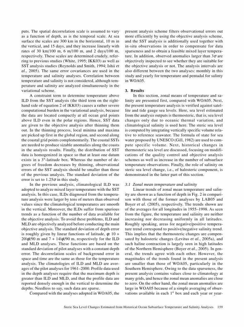
3.1 Zonal mean temperature and salinityLinear trends of zonal mean temperature and salin-

ity are shown as a function of depth in Fig. 2 in compari-son with those of the former analyses by LAB05 andBoyer et al. (2005), respectively. The trends shown areof the averages for all longitudes in 1955–1998. As seenfrom the figure, the temperature and salinity are neitherincreasing nor decreasing uniformly in all latitudes.Roughly speaking, areas for negative/positive tempera-ture trend correspond to positive/negative salinity trend.This implies that the thermosteric changes are compen-sated by halosteric changes (Levitus et al., 2005a), andsuch haline contraction is largely seen in high latitudesof the Northern Hemisphere (Boyer et al., 2005). In gen-eral, the trends agree with each other. However, themagnitudes of the trends found in the present analysisare smaller than those of WOA05, particularly in theSouthern Hemisphere. Owing to the data sparseness, thepresent analysis contains values close to climatology atmany grids, and hence the zonal mean anomalies are closeto zero. On the other hand, the zonal mean anomalies arelarge in WOA05 because of a simple averaging of obser-vations available in each 1° box and each year or year-

160 M. Ishii et al.

season compositing period (Subsection 2.3). These dif-ferences in the zonal means are notable and originate fromthe differences in the analysis schemes. The followingsubsection (Subsection 3.3), discusses how the zonal meandifferences affect sea level changes.

3.2 Comparison with satellite and tide gauge sea levelsThe monthly temperature analysis is verified against

a TOPEX/Poseidon SSH analysis by Chambers et al.(2003). In their SSH analysis, a trend of the TOPEX mi-crowave radiometer equipped with the satellite is removedfrom the SSH observations for the period from January1993 to February 1999, and biases caused by the reflec-tion of the radar pulse due to surface waves, so-calledsea state bias, are subtracted from observed SSHs on thebasis of comparison of SSH data with tide gauge data.

Figure 3 shows geographical distributions of corre-lation coefficient (CC; upper) and root mean square dif-ference (RMSD; lower) between thermosteric sea levelof the present analysis (0–700 m depths) and the TOPEX/Poseidon SSH for 1993–2003. Both time series includeseasonal cycles. The present analysis agrees with the SSHanalysis in broad regions with CC exceeding 70% andRMSD less than 4 cm. In general, the agreement is muchbetter in the Northern Hemisphere and the tropical oceans.In the tropics, CC reaches 90%. In Kuroshio and Gulf

Stream regions, RMSDs exceed 5 cm and originate frominsufficient interannual variations in the temperatureanalysis.

The figure is a counterpart of figure 16 of IKK03. Inthe previous comparison, the period was only six yearsfrom 1993 to 1998, the maximum depth of the tempera-ture analysis was 500 m, and the SSH analysis was basedon Kuragano and Shibata (1997) in which meso-scaleeddies are analyzed by using 4-dimensional decorrelationscales that vary geographically. Because of the existenceof meso-scale eddy, RMSDs were more than 15 cm overeddy-active regions such as regions of the Kuroshio,Kuroshio extension, and Gulf Stream. By contrast, theSSH analysis by Chambers et al. (2003) is used in Fig. 3.The eddies are filters out in their SSH analysis. This is aproper choice, since meso-scale eddy is not a target ofthe present analysis.

Shadings in the figure denote if the temperatureanalysis for 1993–1998 agrees with the SSH analysis ornot in comparison with the previous analysis, taking theSSH analysis as reference. The thermosteric sea level iscomputed from temperature analysis and climatologicalsalinity in the upper 500 m since only the temperatureanalysis is available at depths from sea surface to 500 min the previous study. Correlation coefficients of thepresent analysis increase by more than 10% (light shad-

Fig. 2. Trend for zonal means of temperature (upper) and salinity (lower). The trends of the present analyses are shown in theleft-hand panels in comparison with WOA05 (right). The units are 10–3°C/yr and 10–4 psu/yr for temperature and salinitytrends, respectively. Contour interval is 5 in all the panels, and negative trends are shaded.


ing in panel a) in the Southern Hemisphere compared withthe previous study, and root mean square differences be-come smaller by more than 1 cm (light shading in panelb) there as well. Comparing climatology and anomaly ofthe thermosteric sea level with those of SSH separately(figures not shown), half of the changes in the SouthernHemisphere are explained by changes in seasonal cyclesof thermosteric sea level, and the rest by that of theinterannual variations. On the other hand, the presentanalysis becomes worse in some areas (dark shading inpanels a and b) than the previous analysis. More of ob-servations for the 1990s are available in the present analy-sis in comparison with the previous analysis. In regionswhere meso-scale eddies are active, variances of eddy maynot be filtered out in the present analysis as much as inthe SSH analysis. This is because the thermosteric sealevel over some regions in question are in good agree-ment with another SSH analysis in which meso-scale ed-dies are represented. Moreover, temperature variations areoverestimated slightly in data sparse regions, e.g., sealevel averaged over the Indian Ocean and the subtropicsin the Pacific. The SST analysis used in the objective

analysis has small interannual variances over the south-ern oceans compared with that of Reynolds et al. (2002),the latter of which satellite SST observation is used.Owing to this, variability of temperature within isother-mal layer depth becomes small in the present analysis.This results in poor agreement in latitudes south of 50°S.Note that contribution from salinity and freshwater in-puts to sea level changes is not considered in the abovecomparison. However, the better agreement over thesouthern oceans is likely to be due to the increase of ob-served data in WOD01 than in WOD94.

As another verification of the objective analysis,thermosteric sea level is compared with tide gauge dataalong the Japanese coast. Although there are more than100 tidal stations along the coast, long-term records forabout 100 years are available only at 11 stations. Even inobservations of the 11 stations, data suffer from severediscontinuity, or land subsidences and upheavals due toground water extraction and earthquakes. After remov-ing station data unsuitable for the detection of the cli-mate signal, five stations finally remain usable (K.Sakurai, personal communication, 2005). Three stations

Fig. 3. Geographical distribution of a) correlation coefficient (CC; %; upper) and b) root mean square difference (RMSD; cm;lower) between the monthly thermosteric sea level and the TOPEX/Poseidon SSH analysis for 1993–2003. Both time seriesinclude seasonal cycle. The steric sea level is computed from the temperature analysis at depths from surface to 700 m depth.Contour interval in panel a is 20%. Solid contours are for CC of 70% and 90%, and broken for CC of 10%, 30%, and 50%. Inpanel b, counters are drawn every 1 cm by solid and broken lines respectively for RMSDs less than or equal to 4 cm and forRMSDs greater than 4 cm. Shadings denote if the present analysis agrees with the SSH analysis (light shading; increase of CCby 10%; decrease of RMSD by 1 cm) or not (dark shading; decrease of CC by 10%; increase of RMSD by 1 cm), comparedwith the statistics of previous analysis for the period from 1993 to 1998.

162 M. Ishii et al.

of the five are located on the Japan Sea side, with theremainder on the Pacific side. Before comparison withthe thermosteric sea level, crustal movements are elimi-nated from the tide gauge data (see Appendix). The dataof crustal movement are available for 1969–2000. Ac-cordingly, the correction amount in 1969 is applied to databefore 1969, and linearly extrapolated amounts are usedfor 2001–2003. As mentioned above, the sea level dataused here are superior in quality. Hence, the resultant time

series after the correction does not change significantlyin comparison with the time series including crustal move-ment, except for one station on the Pacific side, where atrend due to crustal movement is 0.5 mm/yr.

In Fig. 4, the broken line presents 5-year runningmean sea levels averaged over the above five stations.The sea level decreases from the middle of the last cen-tury, taking a local maximum in the 1970s, and it increasesagain from 1985 to the present. The mean thermostericsea level, which is constructed from grid point values nearthe five tide gauge stations, follows the tide gauge obser-vation well. Although the range of the crustal movementis within one standard deviation of errors estimated forthe steric sea level shown by bars in the figure, the agree-ment becomes better than that for the case of the tidalobservation without the elimination of crustal movement.Because of coarseness of the analysis grid, thethermosteric sea levels are affected by density variationfar away from the coast. For this reason, interannual vari-ations of the Kuroshio path affect the thermosteric sealevels at grid points near the tide gauge stations on thePacific side; for instance, the Kuroshio flowed along largemeander paths in the latter halves of the 1970s and the1980s. The reason for large differences around the mid-1960s is not clear at present. The interdecadal variationof the present analysis is comparable to that of tide gaugedata, while the amplitude of the previous analysis wassmall. This improvement is due to the use of coastal dataas well as the changes in parameters of the quality con-trol procedures in this study.

Improvement of the temperature analysis is seen atother tidal stations worldwide. Figure 5 shows root meansquare difference (RMSD) and correlation coefficient

Fig. 4. Comparison with tide gauge observation along the Japa-nese coast. The broken line indicates long-term tidal obser-vations at 5 station; Oshoro (34.9°N, 132.1°E), Wajima(34.9°N, 132.1°E), Hamada (34.9°N, 132.1°E), Kushimoto(33.5°N, 135.8°E), and Hosojima (32.6°N, 131.7°E). Val-ues are 5-year running mean in mm and relative to 1961–1990 averages. Thermosteric sea levels of the previous andpresent analyses are shown by thin and thick solid lines,respectively. The steric sea level is computed from the tem-perature analysis at depths from surface to 500 m depth.

Fig. 5. Comparison of monthly thermosteric sea level anomalies with monthly tide gauge data at 168 stations where the observa-tions are available for more than 120 months in the period from 1950 to 1998. As shown by the legend in the upper-left corner,symbols denote a combination of correlation coefficient (C) and root mean square difference (R), e.g., open circle meanscorrelation coefficient greater than or equal to 50% and root mean square difference less than or equal to 5 cm. Thresholds50% and 5 cm are close to the averages of the 168 tide gauges. Background contours show annual mean thermosteric sealevels every 10 cm.


(CC) between tide gauge and the thermosteric sea levelsat 168 stations, where tidal data are available for morethan 120 months during the period from 1950 to 1998.The tide gauge data used here are obtained from the Uni-versity of Hawaii Sea Level Center. In low latitudes, CCsare mostly greater than 50%, and in particular the agree-ment is much better in the western and central Pacificaccompanied by RMSDs of less than 5 cm. In contrast,poor agreement is caused by data sparseness and missingsalinity, as discussed in IKK03. At 129 stations out of168, CCs of the present analysis are regarded as statisti-cally significant against those for the previous analysisat the 95% confidence level. Table 1 shows mean CCsand RMSDs for all the stations and for the stations in20°S–20°N in comparison between the present and pre-vious analyses. The present analysis shows good perform-ance as the mean CCs increase by 6%, and the RMSDsreduce by 1–3 mm compared with the previous analysis.Tide gauges whose RMSDs exceed 9 cm are not includedin the above comparison, since they supposedly sufferfrom local effects due to shallow continental shelves orcrustal movement.

3.3 Thermosteric sea level changesFigure 6 shows time series of annual mean

thermosteric sea level averaged in all longitudes alongthree latitudinal bands; 15°N–60°N, 15°S–15°N, 60°S–15°S. The sea level is computed from the temperatureanalysis from surface to 500 m depth. The choice of the500 m depth is for comparison with the previous analysisavailable in the upper 500 m depths.

In the figure, the present analysis (thick solid line)is compared with the previous analysis (thin solid) and atemperature analysis by LAB05 (dotted) for the periodbetween 1955 and 2003, and with a sea surface height(SSH) analysis of TOPEX/Poseidon by Chambers et al.(2003) for 1993–2003 (broken). Error bars in the figure

denote one standard deviation, which are computed fromthe monthly analysis errors available at each grid point.

The thermosteric sea levels vary dominantly ondecadal and interdecadal time scales with periods of 5–20 yrs, and increasing trends are commonly seen in thethree latitudinal bands. As for the northern oceans (panela), the amplitude of the decadal change grows since 1945,and the global mean sea level is rising from the middle of

60°S–60°N 20°S–20°N

CC RMSD CC RMSD

Present analysis 46 57 58 51Previous analysis 40 58 52 54

Table 1. Statistics between thermosteric sea level anomaliesand tide gauge data at stations located in latitudes from 60°Sto 60°N (left-hand columns) and from 20°S to 20°N (right-hand columns). The number of stations is 168 for the formerlatitudinal range and 78 for the latter. The table containscorrelation coefficients (CC in %) and root mean squaredifferences (RMSD in mm) averaged data at all the stationsin each latitudinal range.

Fig. 6. Time series of annual mean thermosteric sea level (mm)averaged along three latitudinal bands; 15°N–60°N, 15°S–15°N, and 60°S–15°S, for years from 1945 to 2003. Thinand thick solid lines indicate the previous and present analy-sis, respectively. Time series of Levitus et al. (2005b) andthe TOPEX/Poseidon SSH analysis by Chambers et al.(2003) are shown respectively by dotted and broken lines.The analysis by Levitus et al. is available from 1955 to 2003,and the SSH data are shown from 1993 to 2003. Thethermosteric sea levels are computed from the temperatureanalysis from sea surface to 500 m depth. All values shownare relative to 1961–1990 averages of each time series. Incase of the TOPEX/Poseidon SSHs, the value in January1993 is adjusted to the mean of thermosteric sea levels ofthe present analysis and Levitus et al.’s. Error bars drawnevery 10 years are of the present analysis and denote errorintervals of one standard deviation.

164 M. Ishii et al.

the 1980s to the end of 2003. Owing to El Niño and South-ern Oscillation, larger interannual changes appear in sealevel in the lower latitudes (panel b) than in other latitu-dinal domains. In the southern oceans (panel c), an in-creasing trend of sea level rise for the entire period isstatistically significant, but is the smallest among the threetime series. The present analysis agrees well with theLAB05 analysis despite many differences between theanalyses schemes adopted by LAB05 and this study.Throughout the period, some discrepancies appear be-

tween the present and the LAB05 analyses, although thesame observational database is used. However, in mostyears, the differences are within the 95% confidence in-terval, that is, about twice as large as those indicated bythe error bar. Year-to-year changes in the thermosteric sealevels are slightly smaller than LAB05’s. Heat content isalso computed from the temperature analyses by integrat-ing the product of specific heat, density, and temperaturevertically. The resultant heat contents show similar curvesto those in Fig. 6.

Although the linear trends of zonal mean tempera-ture are very different in the southern oceans (Fig. 2),small differences are seen between steric sea level ofLevitus et al. (2005a) shown by a dashed line and thepresent analysis (solid). One reason for this is that den-sity is insensitive to temperature change in latitudes southof 50°S where temperature is low. Large variability is seenin year-to-year change in the thermosteric sea level ofLevitus et al. (2005b) over the southern oceans owing tothe variety of vertical temperature anomalies. As a re-sult, the trend of steric sea level is not large, as expectedfrom the temperature trend (Fig. 2b). In contrast, the zonalmean steric sea level of the present analysis increasesrather monotonically (figures not shown). These factsreflect the differences in methodology of the two histori-cal analyses (Section 2). For the reasons mentioned above,

Fig. 7. Trends of zonally averaged thermosteric sea level(mm/yr) for the present analysis (solid line) and Levitus etal. (2005a) (dashed), corresponding to the trends of tem-perature and salinity shown in the Fig. 2.

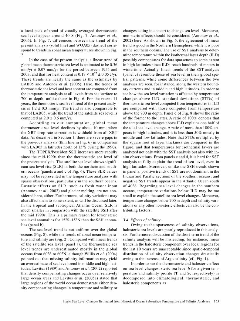
Fig. 8. Geographical distribution of linear trend of a) the satellite sea level (mm/yr), b) thermosteric sea level (mm/yr), andc) SST (10–2°C/yr). Contour intervals are 2.5 mm/yr for sea level and 0.025°C/yr for SST. Light and dark shadings are appliedfor trends of sea level less than –5 mm/yr and greater than 5 mm/yr, respectively, in panels a and b, and for SST trends lessthan –0.05°C/yr and greater than 0.05°C/yr, respectively, in panel c. Contours for trend of zero are not shown, and negativetrends are represented by broken lines. Panel d shows ratio of STDs for thermosteric sea level computed from temperaturewithin isothermal layer depth to those for all the levels. Contours are drawn for 0.25, 0.5, 1, 2, and 4. The period of thestatistics is from 1993 to 2003.


a local peak of trend of zonally averaged thermostericsea level appear around 40°S (Fig. 7; Antonov et al.,2005). In Fig. 7, differences between the trend of thepresent analysis (solid line) and WOA05 (dashed) corre-spond to trends in zonal mean temperatures shown in Fig.2.

In the case of the present analysis, a linear trend ofglobal mean thermosteric sea level is estimated to be 0.36mm/yr ± 0.07 mm/yr for the period between 1955 and2003, and that for heat content is 0.19 × 1022 ± 0.05 J/yr.These trends are nearly the same as the estimates byLAB05 and Antonov et al. (2005). Here, the trends ofthermosteric sea level and heat content are computed fromthe temperature analysis at all levels from sea surface to700 m depth, unlike those in Fig. 6. For the recent 11years, the thermosteric sea level trend of the present analy-sis is 1.2 ± 0.3 mm/yr. The trend is also comparable tothat of LAB05, while the trend of the satellite sea level iscomputed as 2.9 ± 0.6 mm/yr.

According to our computation, global meanthermosteric sea level declines by about 10 mm, whenthe XBT drop rate correction is withheld from all XBTdata. As described in Section 1, there are severe gaps inthe previous analysis (thin line in Fig. 6) in comparisonwith LAB05 in latitudes north of 15°S during the 1990s.

The TOPEX/Poseidon SSH increases more rapidlysince the mid-1990s than the thermosteric sea level ofthe present analysis. The satellite sea level shows signifi-cant sea level rise (SLR) in both the northern and south-ern oceans (panels a and c of Fig. 6). These SLR valuesmay not be represented in the temperature analyses withsparse observations, particularly in the southern oceans.Eustatic effects on SLR, such as fresh water input(Antonov et al., 2002) and glacier melting, are not con-sidered here, either. Furthermore, salinity variations mayalso affect them to some extent, as will be discussed later.In the tropical and subtropical Atlantic Ocean, SLR ismuch smaller in comparison with the satellite SSH afterthe mid 1990s. This is a primary reason for lower stericsea level anomalies for 15°S–15°N than the SSH anoma-lies (panel b).

The sea level trend is not uniform over the globaloceans (Fig. 8), while the trends of zonal mean tempera-ture and salinity are (Fig. 2). Compared with linear trendsof the satellite sea level (panel a), the thermosteric sealevel trends are underestimated mostly in the globaloceans from 60°S to 60°N, although Willis et al. (2004)pointed out that missing salinity information may yieldan overestimate of sea level trend in middle and high lati-tudes. Levitus (1989) and Antonov et al. (2002) reportedthat density compensating changes occur over relativelylarge ocean areas and Levitus et al. (2005a) stated thatlarge regions of the world ocean demonstrate either den-sity compensating changes in temperature and salinity or

changes acting in concert to change sea level. Moreover,non-steric effects should be considered (Antonov et al.,2002) here. As shown in Fig. 6, the agreement of lineartrend is good in the Northern Hemisphere, while it is poorin the southern oceans. The use of SST analysis to deter-mine temperature within the isothermal layer depth (ILD)possibly compensates for data sparseness to some extentin high latitudes since ILDs reach hundreds of meters inwintertime. Actually, linear trends of the SST analysis(panel c) resemble those of sea level in their global spa-tial patterns, while some differences between the twoanalyses are seen, for instance, along the western bound-ary currents and in middle and high latitudes. In order tosee how the sea level variation is affected by temperaturechanges above ILD, standard deviations (STDs) ofthermosteric sea level computed from temperatures in ILDare compared with those computed from temperatureabove the 700 m depth. Panel d of Fig. 8 shows the ratioof the former to the latter. A ratio of 100% denotes thatthe temperature changes above ILD explains one half ofthe total sea level change. A ratio of more than 100% ap-pears in high latitudes, and it is less than 50% mostly inmiddle and low latitudes. Note that STDs multiplied bythe square root of layer thickness are compared in thefigure, and that temperatures for isothermal layers areanalyzed not only with the SST analysis but also with in-situ observations. From panels c and d, it is hard for SSTanalysis to fully explain the trend of sea level, even inhigh latitudes. Moreover, unlike the SSH trends shownin panel a, positive trends of SST are not dominant in theIndian and Pacific sections of the southern oceans, andnegative SST trends appear in the Atlantic Ocean southof 40°S. Regarding sea level changes in the southernoceans, temperature variations below ILD may be toosmall to explain the satellite sea level changes. Moreover,temperature changes below 700 m depth and salinity vari-ations or any other non-steric effects can also be the con-tributing factors.

3.4 Effects of salinityOwing to the sparseness of salinity observations,

halosteric sea levels are poorly reproduced in this analy-sis. Furthermore, discussion of the short-term trend of thesalinity analysis will be misleading; for instance, lineartrends in the halosteric component over local regions forthe last 10 years are unacceptable since spatio-temporaldistribution of salinity observation changes drasticallyowing to the increase of Argo salinity (cf., Fig. 1).

In order to see the thermosteric and halosteric effecton sea level changes, steric sea level h for a given tem-perature and salinity profile (T and S, respectively) isdecomposed into climatological, thermosteric, andhalosteric components as

166 M. Ishii et al.

h hv

TT T z

v

SS S z

c c k

kk T T

S S

k kc

k

k

kk T T

S S

k kc

k

k kc

k kc

k kc

k kc

T S T S, ,( ) = ( ) + ∂∂

−( )

+ ∂∂

−( )

∑

∑

==

==

δ

δ

by linearization about a climatological temperature andsalinity profile (Tc and Sc, respectively), where suffix kindicates the vertical level number, vk is specific volumecomputed from local temperature and salinity, and the δzkdenotes layer thickness. This approach is similar to thatof Antonov et al. (2002). After computing the thermostericand halosteric components from the monthly temperatureand salinity analyses, standard deviations (STDs) of thethermosteric and halosteric components for 1961–2000are compared. Here, temperature and salinityclimatologies are the averages of the analyses for 1961–2000. Figure 9 shows the ratio of halosteric STD tothermosteric STD nearly over the global oceans. The com-putation of STDs was done using the analyses only atgrid points with neighboring observations available in themonthly analysis, that is, where the analysis errors of tem-perature and salinity are reduced at least by 2.5% at allthe depths from the standard deviation of background er-ror.

A meridional contrast and some characteristic fea-tures are apparently seen in the figure; the thermostericcomponent is dominant in low latitudes, especially in thetropical and subtropical regions of the Pacific and IndianOceans, while the halosteric STDs exceeds thermostericSTDs in high latitudes, particularly along sea-ice mar-

gins and closed seas (dark shades). In addition, the roleof salinity on steric changes appears to be more impor-tant in the Atlantic Ocean than in other oceans since theratio is about 0.5 broadly, even in the tropical and sub-tropical Atlantic Ocean, and less than or about 0.2 overother oceans in low latitudes. These patterns reflect ver-tical patterns of temperature and salinity variations andof climatological states in each region. The figure sug-gests an intrinsic role of salinity on sea level change. InFig. 3, root mean square differences normalized by thestandard deviation of interannual SSH anomaly are largein high latitudes and over the Atlantic Ocean rather thanin other oceans (additional figures not shown). Therefore,the halosteric component should not be ignored when dis-cussing steric sea levels distributed geographically, asdone in Figs. 3 and 8. A similar image to that in the figurecan be obtained by computing directly from observed tem-perature and salinity profiles. However, the result will bemuch more noisy than that shown in the figure.

In order to see how much the halosteric componentaffects global mean steric sea level, the time series of thehalosteric component is compared with that of thethermosteric component (Fig. 10). The values plotted areaverages in all longitudes from 60°S to 60°N. Unlike thestatistics shown in Fig. 9, the steric sea levels at all thegrid points are used in averaging. The global mean stericsea level appears to be determined primarily by thethermosteric component. This result is the same as thatreported by Antonov et al. (2002). The linear trend ofthermosteric and halosteric components for 1954–2003is 0.31 ± 0.07 mm/yr and 0.04 ± 0.01 mm/yr, respectively.These estimates are close to those of WOA05 producedby Levitus et al. (2005b) and Boyer et al. (2005), respec-tively. Note that the salinity analysis is close to climatol-

Fig. 9. Ratio of halosteric component to thermosteric component. Contours drawn are of ratio 0.1, 0.2, 0.5, 1, 2, 5, and light anddark shades indicate ratio less than 0.2 and greater than 1, respectively. Sparse sampling areas are shown by shading withmoderate darkness.


ogy widely in the global oceans for all the period, exceptafter 2001. In the above estimate, the halosteric trend is10 times smaller than thermosteric trend. Meanwhile,negative trends of salinity should be caused by sourcesof freshwater other than melting sea ice, and additions offreshwater to the oceans result in sea level rise. AsAntonov et al. (2002) pointed out, sea level rise due toadditions of freshwater to the global oceans, which areequivalent to observed salinity changes, are substantial.

4. Concluding RemarksThe objective analysis of monthly temperature and

salinity has been carried out with the aim of reproducingthe spatial distribution of the variables and their localchanges on interannual and interdecadal time scales.Steric sea level changes are mainly discussed using themonthly subsurface temperature and salinity analysiswhich is a revised version of Ishii et al. (2003). The analy-ses are carried out using the variational minimizationscheme with the World Ocean Data 2001 edition, IRDsea surface salinity data, and the SST analysis of Ishii etal. (2005). The present analysis covers the topmost 700m of the global ocean from 1945 to 2003. The analysisand quality control schemes are mostly the same as thoseof the previous analysis, except for minor changes in qual-ity control and data selection procedures. The drop ratecorrection has been applied to XBT data that are subjectto the correction. Without the correction, a significant gapof about ten millimeters appears in the global meanthermosteric sea level as in the previous analysis. Thenew monthly analysis presents reasonable global meanvariations of steric sea level for recent 59 years. Use ofobservations near coasts yields realistic fluctuations ofthe analyzed temperatures.

The trends of steric sea level estimated from thepresent analysis are comparable to WOA05 by Boyer etal. (2005) and Antonov et al. (2005). The analyzed fields

Fig. 10. Time series of the monthly halosteric (thick) andthermosteric (thin) components averaged in all longitudesfrom 60°S to 60°N.

of temperature and salinity are generally smooth ratherthan those of WOA05, since the quality control and analy-sis schemes adopted in this study are constructed so as tofilter out observational noise more than in WOA05. Inaddition, the linear trends of zonally averaged tempera-ture and salinity are smaller than theirs. A large discrep-ancy is found in the time series during the recent 11 yearsbetween the thermosteric sea level and the satellite seasurface height (SSH), especially in the southern oceans.The thermosteric trends may be underestimated in thesouthern oceans owing to data sparseness (Lombard etal., 2005). Salinity variability is one of the contributingfactors in steric sea level, in particular, in high latitudesand the Atlantic Ocean according to the estimation of thisstudy (Fig. 9). The SST variations in high latitudes affectsea level changes largely since the mixed layer depth isgreat; they explain more than 50% of the standard devia-tion of thermosteric sea level variation at latitudes greaterthan 50° (Fig. 8). However, the geographical patterns ofSST trend are not necessarily the same as those of sealevel. Part of the differences of thermosteric sea level fromSSH (Fig. 6) may be caused by insufficient representa-tion around the Antarctic Circumpolar Current (ACC).Gille (2002) reported warming at a rate of 0.004°C/yr onaverage in 700–1100 m along ACC from the 1950s to the1980s. This layer is not the target of the present objectiveanalysis. When temperature increases by 0.1°C from cli-matology uniformly in this layer, thermosteric sea levelwould rise by about 5 mm.

In turn, non-steric effects should be considered whencomparing steric sea level with tide gauge data and SSHobservations. Recent publications (Antonov et al., 2002;Levitus et al., 2005a) have proposed a guideline to inter-pret underestimation of thermosteric sea level against sealevel rise detected by tide gauge and the SSH data. If thetemperature and salinity analyses were true, non-stericcomponents would be significantly large in the southernoceans (Fig. 6). However, there is no answer to this atpresent, including spatial distributions of non-steric com-ponents. Further investigation is needed for quantitativeunderstanding of sea level variations over each oceanbasin.

In this study, local changes in the thermosteric sealevel are compared with the tide gauge data along the Japa-nese coast, eliminating crustal movement from 1969 to2003. The comparison shows that the thermosteric com-ponent is dominant in the sea level change around Japan.As for tide gauges in the global oceans, the agreement isbetter in areas where the thermosteric components areregarded as a dominant factor in steric sea level changeas shown in Fig. 9. In the mean time, tide gauge data areuseful for discussions of secular change in sea level andare actually utilized in a number of climate studies. How-ever, any discussion of them should take care to account

168 M. Ishii et al.

for crustal movement, at least in the Japanese tide gauges.At several stations used in Fig. 4, differences betweenthermosteric sea level and tide gauge data are large be-fore 1969, possibly because the data of crustal movementare not available.

The new data set contains analysis errors as well asanalyzed values, as did the previous data set. It is hopedthat the analysis is applicable to studies to detect long-term variability in the global oceans, such as global warm-ing and sea level rise. There still remains room for im-provement in the objective analysis. In order to producemonth-to-month persistent anomalies and more spatio-temporal variability, it may be effective to use analysis atthe previous time step as the first guess, as Reynolds andSmith (1994) did.

AcknowledgementsThe authors wish to thank the distributors of WOD01

and climatologies and anomaly fields of WOA05 (Dr.Levitus, NODC/NOAA/USA; http://www.nodc.noaa.gov/),the TOPEX/Poseidon SSH analysis (CSR, the Universityof Texas, USA; http://www.csr.utexas.edu/sst/), and tidegauge data (the University of Hawaii Sea Level Center;http://www.soest.hawaii.edu/kilonsky/uhslc.html). Theyappreciate the excellent investigation of the previousanalysis by Drs. A. Cazenave and A. Lombard (CNES/France), who provided many hints for improvement ofthe analysis. Their appreciation is extended to Mr. K.Sakurai (Office of Marine Prediction, JMA) for valuableinformation on the sea level changes along the Japanesecoast. Prof. Hanawa (Tohoku Univ.) encouraged the au-thors in completing the manuscript. The thoughtful andconstructive comments of two anonymous reviewers arethankfully acknowledged. This work was partially sup-ported by the Japan Science and Technology Agency

through the Core Research for Evolutional Science andTechnology.

Appendix. Elimination of Crustal MovementIn Japan, tide level is presented as a value measured

from the datum line (DL) fixed at each tide gauge. DL isconnected to the Japan Datum of Leveling, that is, theorigin of ground leveling of Japan, via close sea benchmarks and fixed points of tide gauges (Fig. A1) As tidegauges are constructed on the ground, the presented tidevalues contain effects of crustal movements and oceanicorigin sea level changes. Japan is located in a geologi-cally highly active region. To reduce the crustal move-ment effects, ground leveling has been done every 5 or 6years on average from fixed points to close sea benchmarks. Ordinarily, the distances from fixed points to closesea bench marks are 2–6 km. But, the distance from theJapan Datum of Leveling to close sea bench marks issometimes over 1000 km. So the heights of close seabench marks are not revised very frequently because thecompilation of ground leveling data needs much time.Actually, the latest revision was made by the GeologicalSurvey of Japan in 2000 and the second latest one wasmade in 1969. But the ground leveling has been donecontinuously and the results are compiled as Height Dif-ference Data. We made calculations to get time series ofheight of close sea bench marks using Height DifferenceData directly. To minimize errors, we took a loop routefor the calculations and fixed error criteria as 2.5S1/2 mm,where S is the distance measured along the loop route inkm. If the height difference of a bench mark at the begin-ning and after the calculation along the loop route is overthe criteria, we adopt another loop route until the errormeets the criteria. The total amount of error is distrib-uted to the bench marks’ height of the loop route propor-

Fig. A1. Relationship between leveling bench marks and tide gauge observation. See text for details.


tionally to the distance of the bench marks along the looproute. These calculations were made all around Japan andthe time series of the height of close sea bench markswere determined.

ReferencesAntonov, J. I., S. Levitus and T. P. Boyer (2002): Steric sea

level variations during 1957–1994: Importance of salinity.J. Geophys. Res . , 107(C12), 8013, doi:10.1029/2001JC000964.

Antonov, J. I., S. Levitus and T. P. Boyer (2005): Thermostericsea level rise, 1955–2003. Geophys. Res. Lett., 32, L12602,doi:10.1029/2005GL023112.

Boyer, T. P. and S. Levitus (1994): Quality Control and Process-ing of Historical Oceanographic Temperature, Salinity, andOxygen Data. NOAA Technical Report NESDIS 81, 64 pp.

Boyer, T. P., M. E. Conkright, J. I. Antonov, O. K. Baranova,H. Garcia, R. Gelfeld, D. Johnson, R. Locarnini, P. Murphy,T. O. Brien, I. Smolyar and C. Stephens (2001): WorldOcean Database 2001, Volume 2: Temporal Distribution ofBathythermograph Profiles. NOAA Atlas NESDIS 43, 119pp., CD-ROM, U.S. Government Printing Office, Washing-ton, D.C.

Boyer, T. P., S. Levitus, J. I. Antonov, R. A. Locarnini and H.E. Garcia (2005): Linear trends in salinity for the WorldOcean, 1955–1998. Geophys. Res. Lett., 32, L01604,doi:10.1029/2004GL021791.

Cazenave, A. and R. S. Nerem (2004): Present-day sea levelchange: observations and cause. Rev. Geophys., 42, RG3001,doi:10.1029/2003RG000139.

Chambers, D. P., S. A. Hayes, J. C. Ries and T. J. Urban (2003):New TOPEX sea state bias models and their effect on glo-bal mean sea level. J. Geophys. Res., 108(C10), 3305,doi:10.1029/2003JC001839.

Church, J., J. M. Gregory, P. Huybrechts, M. Kuhn, K. Lambeck,M. T. Nhuan, D. Qin and P. L. Woodworth (2001): Changesin sea level. In Climate Change 2001: The Scientific Basis,Contribution of Working Group I to the Third AssessmentReport of the Intergovernmental Panel on Climate Change,ed. by J. T. Houghton et al., Cambridge Univ. Press, NewYork.

Conkright, M. E., R. A. Locarnini, H. E. Garcia, T. D. O. Brien,T. P. Boyer, C. Stephens and J. I. Antonov (2001): WorldOcean Atlas 2001: Objective Analyses, Data Statistics, andFigures. NOAA Atlas NESDIS 42, 17 pp., CD-ROM, U.S.Government Printing Office, Washington, D.C.

Derber, J. C. and A. Rosati (1989): A global oceanic data as-similation technique. J. Phys. Oceanogr., 19, 1333–1347.

Douglas, B. C. and W. R. Peltier (2002): The puzzle of globalsea level rise. Phys. Today, 55, 35–40.

Ghil, M. and P. Malanotte-Rizzoli (1991): Data Assimilationin Meteorology and Oceanography. Advances in GEO-PHYSICS, Vol. 33, Academic Press, p. 141–266.

Gill, A. E. (1982): Atmosphere-Ocean Dynamics. InternationalGeophysics Series, Academic Press.

Gille, S. (2002): Warming of the southern ocean since the 1950s.Science, 295, 1275–1277.

Hanawa, K., P. Raul, R. Bailey, A. Sy and M. Szabados (1995):

A new depth-time equation for Sippican or TSK T-7, T-6,and T-4 expendable bathythermographs (XBTs). Deep-SesRes., 42, 1423–1451.

Hansen, D. V. and W. C. Thacker (1999): Estimation of salinityprofiles in the upper ocean. J. Geophys. Res., 104(C4),7921–7933.

Ishii, M., M. Kimoto and M. Kachi (2003): Historical oceansubsurface temperature analysis with error estimates. Mon.Wea. Rev., 131, 51–73.

Ishii, M., A. Shouji, S. Sugimoto and T. Matsumoto (2005):Objective analyses of SST and marine meteorological vari-ables for the 20th century using ICOADS and the KobeCollection. Int. J. Climatol., 25, 865–879.

Kuragano, T. and A. Shibata (1997): Sea surface dynamic heightof the Pacific Ocean derived from TOPEX/POSEIDON al-t imeter data: Calculation method and accuracy. J.Oceanogr., 53, 585–599.

Levitus, S. (1982): Climatological Atlas of The World Ocean.NOAA Prof. Paper No. 13, 173 pp., U.S. Government Print-ing Office, Washington, D.C.

Levitus, S. (1989): Interpentadal variability of temperature andsalinity at intermediate depths of the north Atlantic Ocean,1970–74 versus 1955–1959. J. Geophys. Res., 94(C5),6091–6131.

Levitus, S., C. Stephens, J. I. Antonov and T. P. Boyer (2000):Yearly and Year—Season Upper Ocean TemperatureAnomaly Fields, 1948–1998. NOAA Atlas NESDIS 40(available from http://www.nodc.noaa.gov/OC5/PDF/AT-LAS/nesdis40.pdf).

Levitus, S., J. I. Antonov, T. P. Boyer, H. E. Garcia and R. A.Locarnini (2005a): Linear trends of zonally averagedthermosteric, halosteric, and total seteric sea level for indi-vidual ocean basins and the world ocean, (1955–1959)–(1994–1998). Geophys. Res. Lett., 32, L16601, doi:10.1029/2005GL023761.

Levitus, S., J. I. Antonov and T. P. Boyer (2005b): Warming ofthe world ocean, 1955–2003. Geophys. Res. Lett., 32,L02604, doi:10.1029/2004GL021592.

Lombard, A., A. Cazenave, P.-Y. Le Traon and M. Ishii (2005):Comtribution of thermal expansion to present-day sea-levelchange revisited. Global and Planetary Change, 47, 1–16.

Maes, C. and D. Behringer (2000): Using satellite-derived sealevel and temperature profiles for determining the salinityvariability: A new approach. J. Geophys. Res., 105(C4),8537–8457.

Peltier, W. R. (2001): Global isostatic adjustment and moderninstrumental records of relative sea level history, Chapter4. In Sea Level Rise: History and Consequences, ed. by B.C. Douglas, M. S. Kearney and S. P. Leatherman, AcademicPress, New York.

Reynolds, R. W. and T. M. Smith (1994): Improved global seasurface temperature analyses using optimum interpolation.J. Climate, 7, 929–948.

Reynolds, R. W., N. A. Rayner, T. M. Smith, D. C. Stokes andW. Wang (2002): An improved in-situ and satellite SSTanalysis for climate. J. Climate, 15, 1609–1625.

Stephens, C., S. Levitus, J. I. Antonov and T. P. Boyer (2001):The Pacific regime shift. Geophys. Res. Lett., 28, 3721–3724.

170 M. Ishii et al.

The Argo Science Team (1999): ARGO: The global array pro-filing floats. In Proceedings of the OOPC/UDP Ocean ObsConference, Saint Raphaël, France, 18–22 October, 1999,12 pp.

Vossepoel, F. C., R. W. Reynolds and L. Miller (1999): Use ofsea level observations to estimate salinity variability in thetropical Pacific. J. Atmos. Ocean. Tech., 16, 1401–1415.

White, W. B. (1995): Design of a global observing system forgyre-scale upper ocean temperature variability. Prog.Oceanogr., 36, 169–217.

Willis, J. K., D. Roemmich and B. Cornuelle (2004): Interannualvariability in upper ocean heat content, temperature, andthermosteric expansion on global scales. J. Geophys. Res.,109, C12036, doi:10.1029/2003JC002260.

steric sea level changes estimated from historical ocean

Documents