stiffness variation in hockey sticks and the impact on...
TRANSCRIPT

1
THE UNIVERSITY OF BIRMINGHAM
Department of Metallurgy and Materials
Stiffness variation in hockey sticks and the
impact on stick performance
Graeme Nigel Carlisle
788002
Submitted for the degree of
Masters of Research – Science and Engineering of Materials
August 2011
Department of Metallurgy and Materials

University of Birmingham Research Archive
e-theses repository This unpublished thesis/dissertation is copyright of the author and/or third parties. The intellectual property rights of the author or third parties in respect of this work are as defined by The Copyright Designs and Patents Act 1988 or as modified by any successor legislation. Any use made of information contained in this thesis/dissertation must be in accordance with that legislation and must be properly acknowledged. Further distribution or reproduction in any format is prohibited without the permission of the copyright holder.
2
Stiffness variation in hockey sticks and the impact on stick
performance
Graeme Nigel Carlisle
Submitted with corrections for the degree of
Masters of Research – Science and Engineering of Materials
August 2011
Multiple sectioned shafts of carbon fibre composite were modelled using Composite Design
Analysis software in order to replicate the range of flexural rigidities shown across the
current field hockey stick market. The shafts were then manufactured using hand lay-up
and hot-pressing techniques, tested under static and dynamic conditions and the goodness
of their relationship with the modelled behaviour was assessed. The shafts were also
analysed microscopically for volume fraction, ply-orientation and the interaction between
the varied lay-up sections.
The modelling gave a good understanding of the trend of behaviour that was to be
expected, but was not accurate enough to predict experimental values. It is possible to
create multiple sectioned CFRP shafts that can be controlled for overall flexural rigidity and
also strain distribution or “kick-point”. The hand lay-up and hot pressing technique
produces consistent volume fraction and accurate fibre orientation, however the seams at
which the sections join requires further investigation and development. The relationship
between stick stiffness and ball speed validated previous research, stiffer shafts produced a
higher CoR in the drop ball test.
There is scope to introduce this stiffness control of the bending behaviour into hockey
sticks, by either material properties or section moment of area.
Keywords: CFRP, Field Hockey, CoDA Modelling, Composite Manufacture Techniques.

3
Contents
Abstract 2
Nomenclature 5
1 Introduction ................................................................................................................................... 6 1.1 History of the game ............................................................................................................................ 6 1.2 Equipment function and FIH rules ............................................................................................... 9
1.2.1 The stick ............................................................................................................................................................ 9 1.2.2 The ball ............................................................................................................................................................ 11
1.3 Composite materials ...................................................................................................................... 12 1.3.1 Polymer matrix composites .................................................................................................................... 12 1.3.2 Modulus of unidirectional composites and laminates ................................................................. 12
1.4 Modification of stiffness ................................................................................................................ 14 1.5 Aims and Objectives ....................................................................................................................... 19
2 Modelling of shaft behaviour ................................................................................................. 20 2.1 Introduction ...................................................................................................................................... 20 2.2 Methodology ...................................................................................................................................... 20 2.3 Results and discussion................................................................................................................... 24
3 Preliminary Panel analysis ..................................................................................................... 26 3.1 Methodology ...................................................................................................................................... 26
3.1.1 Quasi-static flexure ..................................................................................................................................... 26 3.1.2 Optical analysis ............................................................................................................................................ 27
3.2 Results and Discussion .................................................................................................................. 28 3.2.1 Quasi-static flexure ..................................................................................................................................... 28 3.2.2 Optical analysis ............................................................................................................................................ 28
4 Control shafts ............................................................................................................................... 32 4.1 Methodology ...................................................................................................................................... 32
4.1.1 Manufacture .................................................................................................................................................. 33 4.1.2 Dimensions .................................................................................................................................................... 33 4.1.3 Optical analysis ............................................................................................................................................ 34 4.1.4 Quasi-static shaft flexure.......................................................................................................................... 34
4.2 Results and Discussion .................................................................................................................. 35 4.2.1 Dimensions .................................................................................................................................................... 35 4.2.2 Optical analysis ............................................................................................................................................ 36 4.2.3 Quasi-static shaft flexure.......................................................................................................................... 37
5 Multiple section shafts .............................................................................................................. 38 5.1 Methodology ...................................................................................................................................... 38
5.1.1 Manufacture .................................................................................................................................................. 38 5.1.2 Hot pressing .................................................................................................................................................. 39 5.1.3 Dimensions .................................................................................................................................................... 40 5.1.4 Quasi-static shaft flexure.......................................................................................................................... 41 5.1.5 Dynamic drop-ball shaft flexure............................................................................................................ 42 5.1.6 Strain distribution ....................................................................................................................................... 44 5.1.7 Optical analysis ............................................................................................................................................ 45
5.2 Results and Discussion .................................................................................................................. 46

4
5.2.1 Dimensions .................................................................................................................................................... 46 5.2.2 Quasi-static shaft flexure.......................................................................................................................... 48 5.2.3 Dynamic drop-ball shaft flexure............................................................................................................ 54 5.2.4 Strain distribution ....................................................................................................................................... 56
5.3 Optical analysis ................................................................................................................................ 62
6 Conclusions ................................................................................................................................... 71
7 References ..................................................................................................................................... 72

5
Nomenclature
FIH Federation Internationale d’Hockey
I Second moment of area
PMC Polymer matrix composites
CFRP Carbon fibre reinforced polymer
GFRP Glass fibre reinforced polymer
EI Flexural rigidity
UD Uni-directional
E11 The elastic modulus in the ‘1’ or longitudinal direction
E22 The elastic modulus in the ‘2’ or transverse direction
G12 The shear modulus in the 1-2 axes
ν12 The ‘major’ Poisson’s ratio
ν21 The ‘minor’ Poisson’s ratio
CoDA Component design analysis
F Force
L Length
δ Deflection
M Moment
Q Stiffness
a Acceleration
v Final velocity at maximum deflection i.e. Rest
u Impact velocity
t Time from impact to maximum deflection
M Mass of hockey ball
CoR Coefficient of restitution
ƒ1 Mode 1 bending frequency
C1 3.52
m0 ρ / A
ρ Density
A Section area
6
1 Introduction
1.1 History of the game
Evidence of a game similar to hockey has been found in tomb drawings in the Nile valley
Egypt, dating back to 4,000 years ago. It then appeared again, during the middle ages
throughout Europe, having various names like camocke (England) or shinty (Scotland). The
modern game of hockey was however, developed in the public schools of England during
the early 19th century. It then spread across Middlesex cricket clubs, such as Teddington, as
a winter training exercise; much preferred to football. The game was played with an old
cricket ball, using wooden sticks on the smooth cricket outfield. Basic rules including
restriction of the backswing to lower than shoulder height and only being able to score
inside a semi-circle in front of the goal, known as the “D” were introduced and in 1886 the
Hockey Association was formed. The growth of hockey throughout the United Kingdom
was rather sporadic as clubs from different regions often did not agree on rules. The
introduction of hockey all over the British Empire during the late 19th century led to the
first international competition between Ireland and Wales in 1895, the same year in which
the International Rules Board was founded. Hockey first appeared in the Olympic Games in
1908 and became a permanent fixture in the Amsterdam games of 1928. By this time
European countries played under a single structure or governing body known as the FIH
(Fédération Internationale d‘Hockey); the FIH is now a worldwide body, having 112
member states.
A major development in the game came with introduction of ‘synthetic turf’ in the 1970s;
this led to a rapid increase in the speed at which the game was played and, to some extent,
a loss of some skills, such as vertical stick stopping due to the predictability of the playing
surface. The change in playing surface also led to a significant change in the design of the
equipment, tactics and techniques used during play.
7
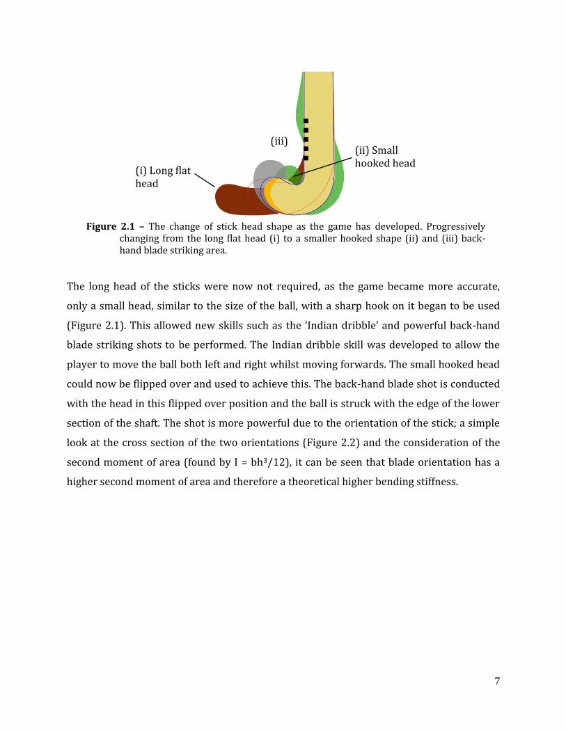
The long head of the sticks were now not required, as the game became more accurate,
only a small head, similar to the size of the ball, with a sharp hook on it began to be used
(Figure 2.1). This allowed new skills such as the ‘Indian dribble’ and powerful back-hand
blade striking shots to be performed. The Indian dribble skill was developed to allow the
player to move the ball both left and right whilst moving forwards. The small hooked head
could now be flipped over and used to achieve this. The back-hand blade shot is conducted
with the head in this flipped over position and the ball is struck with the edge of the lower
section of the shaft. The shot is more powerful due to the orientation of the stick; a simple
look at the cross section of the two orientations (Figure 2.2) and the consideration of the
second moment of area (found by I = bh3/12), it can be seen that blade orientation has a
higher second moment of area and therefore a theoretical higher bending stiffness.
(i) Long flat head
(ii) Small hooked head
(iii)
Figure 2.1 – The change of stick head shape as the game has developed. Progressively changing from the long flat head (i) to a smaller hooked shape (ii) and (iii) back-hand blade striking area.

8
The construction of both the sticks and balls was developed in order to keep up with the
new pace of the game. Sticks, originally made of mulberry now started to be made from
composite materials, such as glass; carbon; and kevlar continuous fibre reinforced
polymers and areas of discontinuous fibre reinforcements. The extra stiffness that the use
of these materials gave the sticks was suited to a faster, more powerful game, however
many players still prefer the ‘feel’ or ‘comfort’ they gain from the more compliant wooden
sticks, allowing them to stop and control the ball more easily (McHutchon et al., 2004). The
old cricket balls became unsuitable for the water-based synthetic pitches as water
absorption contributes to swelling of the cork core and creates a non-spherical cross-
section, leading to inconsistent rolling behaviour. Hockey balls are now an example of solid
ball construction being composed of mixtures of cork, wool and elastomer with a
polyurethane (PU) or polyvinyl chloride (PVC) cover (Ranga et al., 2008). The PU/PVC
cover creates a seal around the water absorbing core materials and prevents the swelling
and asymmetry found in cricket balls. The dimpled polymer cover, without the seam of
leather cricket balls improved roll due to the completely spherical shape and aerodynamic
consistency due to the stabilising affect the laminar flow around the ball created by the
dimples, by delaying the occurrence of the separation of the flow, creating a smaller wake
and therefore significantly less drag (Beasley and Camp, 2002).
Since its foundation in 1924 the FIH has been constantly reviewing and updating the
regulations of the game. The premise of the game is now that two teams of eleven have to
Figure 2.2 – Hockey stick cross sections in the (i) normal and (ii) blade orientations.
(i) (ii)
h
b
b

9
negotiate a small polymer, cork and elastomer composite layered ball into a goal, using
only the flat side of the sharply hooked stick during two halves of 35 minutes duration.
1.2 Equipment function and FIH rules
The constant review and updating of the rules of hockey by the FIH takes into account
developments in surface and equipment technology; the nature of the current game; and, of
course, the safety of participants. The following regulations, which focus on the rules
regarding the stick and ball are taken from the field and equipment chapter of the Rules of
Hockey, sections two and three respectively, published by the FIH, effective from 1st May
2009.
1.2.1 The stick
The hockey stick is used to impact and control the ball and so needs to transfer kinetic
energy over a range of stick head speeds with good directional accuracy. The stick consists
of four distinct sections, the handle (i), a taper (ii) to the blade section (iii) and the sharply
hooked head (iv), (Figure 2.3).
Variables contributing to how a hockey stick feels and performs include the mass, centre of
mass location, shaft stiffness and resistance to twisting. The difficulty comes in achieving a
design that can satisfy the variety of skills used during a game and the preference and
ability of each individual player. In a study on perceived stick performance by McHutchon
et al., (2004) they found that for a hockey hit, all but one player chose a composite stick as
their favourite, 18 out of 26 players chose the least stiff stick as their least favourite and 7
(i) (ii) (iii)
(iv)
Figure 2.3 – Four distinct sections of the modern hockey stick. (i) The handle, (ii) taper from handle to blade, (iii) blade section and (iv) the sharply hooked head.
10
of them also chose the heaviest stick as their least favourite. They found that players were
not able to interpret the correlation between perceived stick power and measured flexural
rigidity (3-point bend, 0.8 m span over the blade section of the stick), but stiffer sticks were
shown to be more powerful. The clamping conditions for both the laboratory and field-
testing were however, different. In a field hockey hit the stick is held with both hands
together at the end of the handle, making the full length of the stick under cantilever
loading during impact. This is inherently different to the way the flexural rigidity was
calculated, under different loading conditions and not taking into account the full span of
the stick. There is therefore, no consideration on which section of the stick dominates the
bending behaviour and how the change in the second moment of area of each section has
an impact on this. The hit is also not a very good indicator of perceived control of the stick
during stopping and dribbling skills as the stick is not put under as much loading and
requires a finer adjustment to technique. When they considered dribbling skills, moment
about the handle, centre of mass, or “pick-up weight” was found to be the most significant
physical parameter and, in fact, the stick with the lowest stiffness, which was a wooden
stick, was preferred by half the participants. This indicates a tradeoff between power and
control of sticks and creates a large range of sticks of composite wrapped wooden sticks
and full composite designs. With both high stiffness composite sticks intended for pure
power and less stiff wooden sticks designed purely for control. Most of the market is
however directed at trying to create a stick that satisfies both these parameters in varying
degrees.
Stick manufacturers classify their sticks in two main ways. The mass of the stick, being
super light, light, medium or heavy and in the power of the stick. Both of which are not
truly comparable quantitatively within or between manufacturers. In McHutchon et al.,
(2006) all tested sticks, all from the same manufacture, were graded as a having a medium
mass, however physical mass ranged between 0.565 kg and 0.618 kg. The power rating
ranged from medium to extra stiff, with no actual measured stiffness values associated with
this. Most of the design parameters are left down to the manufacturer; however the FIH
sets out the following rules and regulations.
Materials:
11
a The stick and possible additions may be made of or contain any material
other than metal or metallic components, provided it is fit for the purpose of
playing hockey and is not hazardous.
b The application of tapes and resins is permitted provided that the stick
surface remains smooth and that it conforms to the stick specifications.
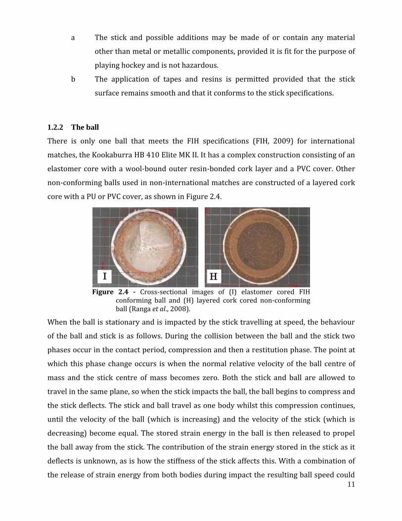
1.2.2 The ball
There is only one ball that meets the FIH specifications (FIH, 2009) for international
matches, the Kookaburra HB 410 Elite MK II. It has a complex construction consisting of an
elastomer core with a wool-bound outer resin-bonded cork layer and a PVC cover. Other
non-conforming balls used in non-international matches are constructed of a layered cork
core with a PU or PVC cover, as shown in Figure 2.4.
When the ball is stationary and is impacted by the stick travelling at speed, the behaviour
of the ball and stick is as follows. During the collision between the ball and the stick two
phases occur in the contact period, compression and then a restitution phase. The point at
which this phase change occurs is when the normal relative velocity of the ball centre of
mass and the stick centre of mass becomes zero. Both the stick and ball are allowed to
travel in the same plane, so when the stick impacts the ball, the ball begins to compress and
the stick deflects. The stick and ball travel as one body whilst this compression continues,
until the velocity of the ball (which is increasing) and the velocity of the stick (which is
decreasing) become equal. The stored strain energy in the ball is then released to propel
the ball away from the stick. The contribution of the strain energy stored in the stick as it
deflects is unknown, as is how the stiffness of the stick affects this. With a combination of
the release of strain energy from both bodies during impact the resulting ball speed could
Figure 2.4 - Cross-sectional images of (I) elastomer cored FIH conforming ball and (H) layered cork cored non-conforming ball (Ranga et al., 2008).
12
theoretically be higher, as the release in strain energy from the ball and stick covert into
kinetic energy transferred to the ball.
1.3 Composite materials
1.3.1 Polymer matrix composites
The majority of polymer matrix composites (PMCs) used in sport consist of a high modulus
or high strength fibre (glass, carbon or Kevlar) in resin (epoxy or phenolic) matrix, the
most commonly used being carbon fibre reinforced polymer (CFRP). The resin matrices
cross-link during curing, which involves the application of heat and pressure via an
autoclave, hot press or vacuum bag. Variation in fibre and resin type along with orientation
and volume fraction are used to control modulus and strength properties along with
anisotropy.
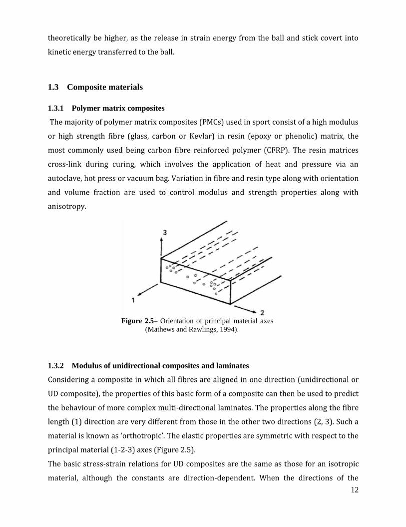
1.3.2 Modulus of unidirectional composites and laminates
Considering a composite in which all fibres are aligned in one direction (unidirectional or
UD composite), the properties of this basic form of a composite can then be used to predict
the behaviour of more complex multi-directional laminates. The properties along the fibre
length (1) direction are very different from those in the other two directions (2, 3). Such a
material is known as ‘orthotropic’. The elastic properties are symmetric with respect to the
principal material (1-2-3) axes (Figure 2.5).
The basic stress-strain relations for UD composites are the same as those for an isotropic
material, although the constants are direction-dependent. When the directions of the
Figure 2.5– Orientation of principal material axes
(Mathews and Rawlings, 1994).
13
applied stresses coincide with the principal (1-2) material axes, strains in terms of stress
are as follows:
where:
E11 = the elastic modulus in the ‘1’ or
longitudinal direction,
E22 = the elastic modulus in the ‘2’ or
transverse direction,
G12 = the shear modulus in the 1-2 axes,
ν12 = the ‘major’ Poisson’s ratio, and
ν21 = the ‘minor’ Poisson’s ratio.
In practical applications, CFRP is not used in single plies and is often not stressed solely
along the longitudinal axis. UD plies are usually stacked in a variety of orientations and
thicknesses to form laminates with the required modulus and strength properties. This
often results in plies where the fibres are no longer aligned parallel to the applied stresses;
these are rotated layers and are subjected to off-axis loading. A number of laminate
theories (Matthews and Rawlings, 1999; Tsai and Hahn, 1980) have been developed to
estimate mechanical properties based on individual ply orientations and properties.
Established convention for denoting both the lay-up and stacking sequence of a laminate is
as follows. For example, a 4-ply laminate, which has the fibre orientation in the sequence
0°, 90°, 90°, 0° from the upper to the lower surface would be shown as (0/90)s. The suffix
‘s’ means that the stacking sequence is symmetric about the mid-thickness of the laminate.
To clarify the laminates (0/45/90)s and (45/90/0)s have the same lay-up, but a different
stacking sequence.
The in-plane modulus of a laminated composite can be obtained directly by applying the
rule of mixtures equation to the modulus of the unidirectional composite and is simply the
arithmetic average of the modulus of the constituent plies. All the information that is
required is the orientation and the volume fraction of each ply group; this will not apply to
off-axis ply containing laminates howe
14
1.4 Modification of stiffness
Investigation into the stiffness of composite sticks, bats and shafts has been carried out
for a number of years relating to various sports (Smith, 2001; Pearsall et al., 1999;
Cheong et al., 2006), in particular for golf shafts (Butler and Winfield, 1994).
The stiffness of a shaft can in theory exert a significant influence on resulting ball
velocity. When an elastic material such as CFRP is deformed, potential energy is stored
in the material in the form of strain energy. This strain energy can then be converted to
kinetic energy at impact, leading to a greater impact speed and hence resultant ball
speed. The ability of the shaft to store and release this energy depends greatly on shaft
stiffness. Optimisation of impact speed in golf drivers, to achieve maximum drive
distance and in field and ice hockey to attain high resultant shot speeds is greatly
desired (Van Gheluwe et al., 1990). The capability of the shaft to maximise this depends
on the conversion of strain energy into kinetic energy and therefore shaft behaviour is
optimised by shaft stiffness. However the mechanics of the impact also affect whether
shaft stiffness must be maximised or more specifically tailored to achieve this.
The stiffness variation along the length of golf shafts and the cause of this variation was
addressed by Huntley (2006) using static and dynamic stiffness analysis over a range of
golf shafts and relating this to microstructural characterisation. The flexural rigidity
distribution was determined using Broulliette’s interpretation of the Euler-Bernoulli
slender beam equation (Broulliette, 2002). The method involved a mass being hung
from the tip, the deflection was then measured for the shaft clamped at progressively
larger distances from the tip. This produces a stiffness profile for the entire length of the
shaft. This study identified the importance of the stiffness distribution on shafts by
documenting three shafts of similar end deflection, yet widely different flexural rigidity
profiles. The flex, or kick point in golf shafts, which is controlled by the degree of taper
and the lay-up of the CFRP, is the point at which maximum deflection occurs and
influences the release of the head into the ball at impact and hence power, trajectory
and accuracy. The head of the golf club can be considered to bend around three
orthogonal axes about the butt or grip end of the shaft, prior to impact. The y-axis is
from the back to the face of the clubhead, the x-axis is from the heel to the toe and some
twisting about the longitudinal z-axis can also occur (Figure 2.6). Deflection about the y-

15
axis occurs in both the lead (positive deflection about neutral z axis) and lag (negative
direction about neutral z axis) directions, whereas deflections about the x-axis occur in
toe-up or toe-down directions about the neutral axis. The degree of deflection in the y-
axis is the only deflection that contributes to clubhead speed, and although deflections
about the x-axis cannot contribute to speed it can have an effect on the trajectory and
accuracy of the ball flight (Figure 2.7).
The flexural rigidity distribution along the shaft therefore has a key role in controlling
the golf shaft’s performance, and so by varying this stiffness along the shaft, different
shaft behaviour can be achieved.
Figure 2.6 – Shaft deflection about three orthogonal
axes prior to impact (MacKenzie, 2005)
Figure 2.7 – Effect of “kick-point” location on ball flight
trajectory (Cheong et al., 2006)
16
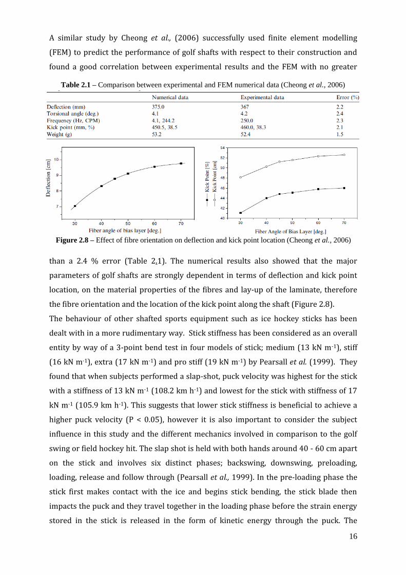
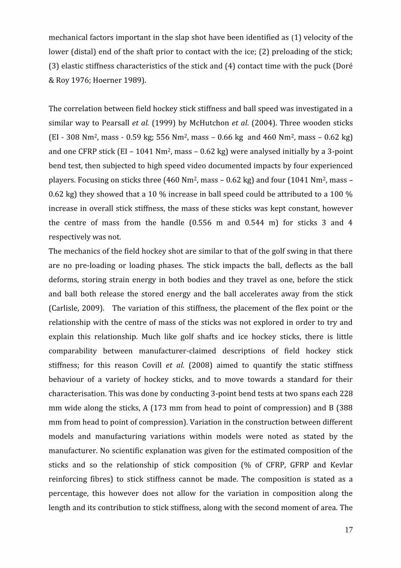
A similar study by Cheong et al., (2006) successfully used finite element modelling
(FEM) to predict the performance of golf shafts with respect to their construction and
found a good correlation between experimental results and the FEM with no greater
than a 2.4 % error (Table 2.1). The numerical results also showed that the major
parameters of golf shafts are strongly dependent in terms of deflection and kick point
location, on the material properties of the fibres and lay-up of the laminate, therefore
the fibre orientation and the location of the kick point along the shaft (Figure 2.8).
The behaviour of other shafted sports equipment such as ice hockey sticks has been
dealt with in a more rudimentary way. Stick stiffness has been considered as an overall
entity by way of a 3-point bend test in four models of stick; medium (13 kN m-1), stiff
(16 kN m-1), extra (17 kN m-1) and pro stiff (19 kN m-1) by Pearsall et al. (1999). They
found that when subjects performed a slap-shot, puck velocity was highest for the stick
with a stiffness of 13 kN m-1 (108.2 km h-1) and lowest for the stick with stiffness of 17
kN m-1 (105.9 km h-1). This suggests that lower stick stiffness is beneficial to achieve a
higher puck velocity (P < 0.05), however it is also important to consider the subject
influence in this study and the different mechanics involved in comparison to the golf
swing or field hockey hit. The slap shot is held with both hands around 40 - 60 cm apart
on the stick and involves six distinct phases; backswing, downswing, preloading,
loading, release and follow through (Pearsall et al., 1999). In the pre-loading phase the
stick first makes contact with the ice and begins stick bending, the stick blade then
impacts the puck and they travel together in the loading phase before the strain energy
stored in the stick is released in the form of kinetic energy through the puck. The
Figure 2.8 – Effect of fibre orientation on deflection and kick point location (Cheong et al., 2006)
Table 2.1 – Comparison between experimental and FEM numerical data (Cheong et al., 2006)
17
mechanical factors important in the slap shot have been identified as (1) velocity of the
lower (distal) end of the shaft prior to contact with the ice; (2) preloading of the stick;
(3) elastic stiffness characteristics of the stick and (4) contact time with the puck (Doré
& Roy 1976; Hoerner 1989).
The correlation between field hockey stick stiffness and ball speed was investigated in a
similar way to Pearsall et al. (1999) by McHutchon et al. (2004). Three wooden sticks
(EI - 308 Nm2, mass - 0.59 kg; 556 Nm2, mass – 0.66 kg and 460 Nm2, mass – 0.62 kg)
and one CFRP stick (EI – 1041 Nm2, mass – 0.62 kg) were analysed initially by a 3-point
bend test, then subjected to high speed video documented impacts by four experienced
players. Focusing on sticks three (460 Nm2, mass – 0.62 kg) and four (1041 Nm2, mass –
0.62 kg) they showed that a 10 % increase in ball speed could be attributed to a 100 %
increase in overall stick stiffness, the mass of these sticks was kept constant, however
the centre of mass from the handle (0.556 m and 0.544 m) for sticks 3 and 4
respectively was not.
The mechanics of the field hockey shot are similar to that of the golf swing in that there
are no pre-loading or loading phases. The stick impacts the ball, deflects as the ball
deforms, storing strain energy in both bodies and they travel as one, before the stick
and ball both release the stored energy and the ball accelerates away from the stick
(Carlisle, 2009). The variation of this stiffness, the placement of the flex point or the
relationship with the centre of mass of the sticks was not explored in order to try and
explain this relationship. Much like golf shafts and ice hockey sticks, there is little
comparability between manufacturer-claimed descriptions of field hockey stick
stiffness; for this reason Covill et al. (2008) aimed to quantify the static stiffness
behaviour of a variety of hockey sticks, and to move towards a standard for their
characterisation. This was done by conducting 3-point bend tests at two spans each 228
mm wide along the sticks, A (173 mm from head to point of compression) and B (388
mm from head to point of compression). Variation in the construction between different
models and manufacturing variations within models were noted as stated by the
manufacturer. No scientific explanation was given for the estimated composition of the
sticks and so the relationship of stick composition (% of CFRP, GFRP and Kevlar
reinforcing fibres) to stick stiffness cannot be made. The composition is stated as a
percentage, this however does not allow for the variation in composition along the
length and its contribution to stick stiffness, along with the second moment of area. The

18
main findings of the study however showed that in all of the sticks tested (9 models, 1 -
6 examples per model) the flexural rigidity closer to the handle (430 – 1069 Nm2) was
greater than in the blade section (310 – 636 Nm2), and that in some cases there was
significant deviation within models (Table 2.2).
Table 2.2 – Variety, mass composition and flexural rigidity of sticks used in Covill et al. (2008).
The construction of a robot capable of swinging hockey sticks at an impact speed of up
to the maximum recorded in-game speed of 46.03 ± 11.58 ms-1 (Rai et al., 2002) by
Carlisle (2009) to investigate the interaction between stick and ball at impact and the
applicability of FIH testing procedures on hockey balls to match scenarios, has the
potential to conduct comprehensive stick testing. This would allow a true analysis
firstly of the variation in static stiffness along the length of a stick using Broulliette’s
equations, how this relates to stick performance and then to the microstructure and
construction of the sticks.
Stick
number
Mass
(g)
Estimated composition Mean
flexural
rigidity
closer to the
handle (B)
(Nm2)
Mean
flexural
rigidity
closer to the
blade (A)
(Nm2)
Carbon
%
Aramid
%
Fibreglass
%
1 603 ± 14 20 20 60 310 ± 13 430 ± 21
2 602 ± 13 30 20 50 329 ± 23 631 ± 35
3 605 ± 33 90 10 - 453 ±19 567 ± 24
4 567 ± 12 35 15 50 410 ± 28 451 ± 65
5 581 85 15 - 505 1069
6 576 85 15 - 387 607
7 564 ± 24 50 5 45 471 ± 28 730 ± 75
8 609 ± 15 50 15 35 552 ± 23 646 ± 29
9 583 ± 9 100 - - 636 ± 30 742 ± 38

19
1.5 Aims and Objectives
Model the behaviour of carbon fibre shafts, with multiple sections along the shaft
of varied fibre orientation to investigate how this affects overall stiffness
behaviour of the shaft.
Manufacture a selection of shafts that represent the overall stiffness of current
hockey stick market found by Covill et al (2008), using hand lay-up and hot
pressing techniques.
Test the shafts under static and dynamic loading conditions and assess their
behaviour in relation to the modelled predictions and behaviour highlighted by
Pearsall et al. (1999) by McHutchon et al. (2004).
Assess the hand lay-up and hot-pressing techniques for volume fraction, ply-
orientation and interaction of varied lay-up sections.
20
2 Modelling of shaft behaviour
2.1 Introduction
In order to produce shafts with the relevant flexural rigidity in comparison to existing
sticks and to understand how to manipulate the lay-up in order to create “kick points”
in the shaft, classic laminate theory was applied to parallel sided shafts. This involved
using CoDA (Component Design Analysis) software and an adapted version of
Brouilette’s equation, resulting in a database of different lay-up, and weak point location
effect on the overall flexural rigidity of composite shafts. From these lay-ups were
selected for fabrication using hot pressing for more detailed analysis.
2.2 Methodology
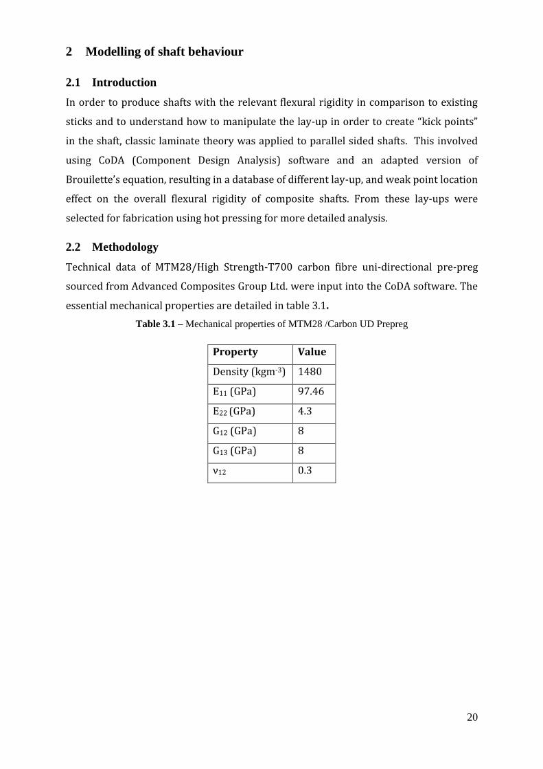
Technical data of MTM28/High Strength-T700 carbon fibre uni-directional pre-preg
sourced from Advanced Composites Group Ltd. were input into the CoDA software. The
essential mechanical properties are detailed in table 3.1.
Table 3.1 – Mechanical properties of MTM28 /Carbon UD Prepreg
Property Value
Density (kgm-3) 1480
E11 (GPa) 97.46
E22 (GPa) 4.3
G12 (GPa) 8
G13 (GPa) 8
ν12 0.3

21
The mechanical properties of the UD prepreg were input into the software to create
plies of the desired properties and orientations so that elastic modulus and moment of
inertia data for different laminates and section dimensions could be predicted. The
CoDA software is limited to applying these data to homogenous laminate beams, and
cannot therefore predict the flexural rigidity of beams with two or more sections of
different lay-ups along its length. To do this Brouilette’s equation (1) for calculating the
flexural rigidity of progressively larger sections of cantilever loaded beams was
manipulated so that it predicted the deflection of known flexural rigidity sections (2);
the stiffness (Q) of the entire shaft made up of different sections can be then be found
and therefore the overall flexural rigidity could be calculated (3)(4).
Where - EI = Flexural rigidity (Nm2)
F = Force (N)
L = Length (m)
δ = Deflection (m)
M = Moment (Nm)
Q = Stiffness (Nm-1)
and
(1)
(2)
(3)
(4)
EI n
l n
EI n-1
l n-1
22
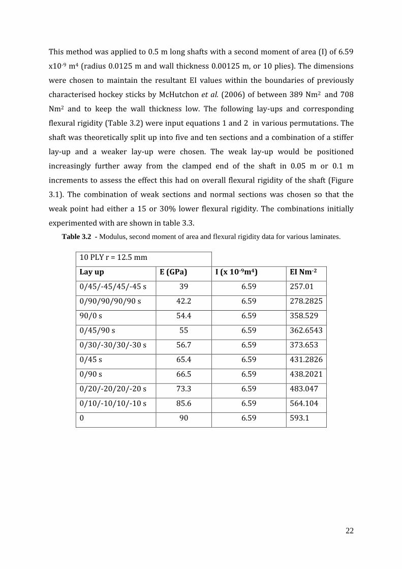
This method was applied to 0.5 m long shafts with a second moment of area (I) of 6.59
x10-9 m4 (radius 0.0125 m and wall thickness 0.00125 m, or 10 plies). The dimensions
were chosen to maintain the resultant EI values within the boundaries of previously
characterised hockey sticks by McHutchon et al. (2006) of between 389 Nm2 and 708
Nm2 and to keep the wall thickness low. The following lay-ups and corresponding
flexural rigidity (Table 3.2) were input equations 1 and 2 in various permutations. The
shaft was theoretically split up into five and ten sections and a combination of a stiffer
lay-up and a weaker lay-up were chosen. The weak lay-up would be positioned
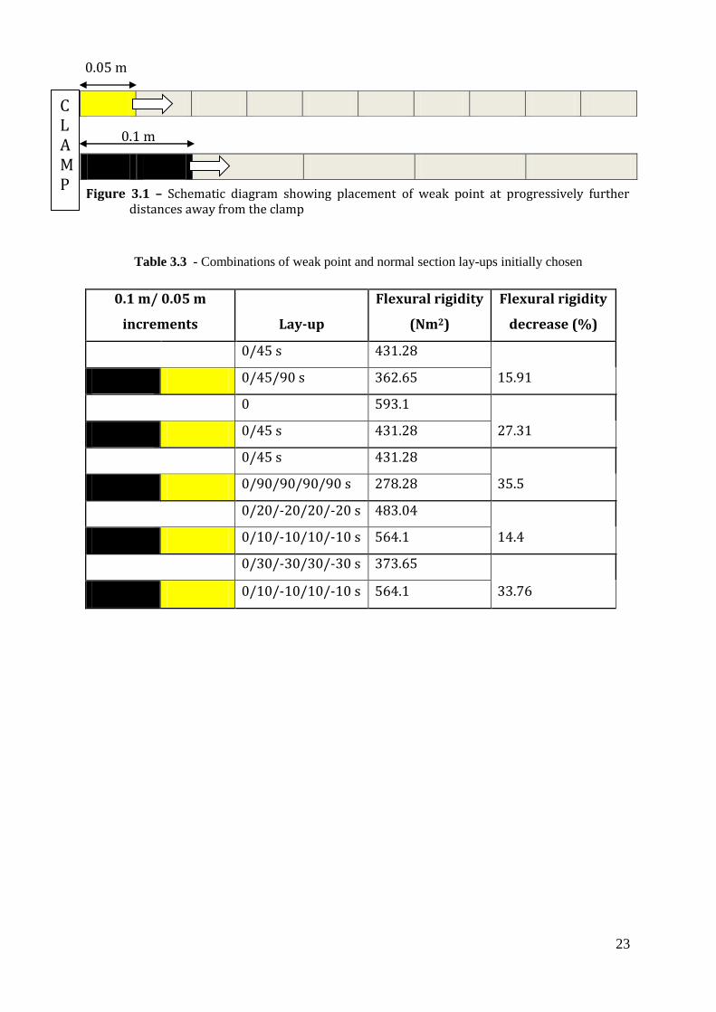
increasingly further away from the clamped end of the shaft in 0.05 m or 0.1 m
increments to assess the effect this had on overall flexural rigidity of the shaft (Figure
3.1). The combination of weak sections and normal sections was chosen so that the
weak point had either a 15 or 30% lower flexural rigidity. The combinations initially
experimented with are shown in table 3.3.
Table 3.2 - Modulus, second moment of area and flexural rigidity data for various laminates.
10 PLY r = 12.5 mm
Lay up E (GPa) I (x 10-9m4) EI Nm-2
0/45/-45/45/-45 s 39 6.59 257.01
0/90/90/90/90 s 42.2 6.59 278.2825
90/0 s 54.4 6.59 358.529
0/45/90 s 55 6.59 362.6543
0/30/-30/30/-30 s 56.7 6.59 373.653
0/45 s 65.4 6.59 431.2826
0/90 s 66.5 6.59 438.2021
0/20/-20/20/-20 s 73.3 6.59 483.047
0/10/-10/10/-10 s 85.6 6.59 564.104
0 90 6.59 593.1
23
Table 3.3 - Combinations of weak point and normal section lay-ups initially chosen
0.1 m/ 0.05 m
increments Lay-up
Flexural rigidity
(Nm2)
Flexural rigidity
decrease (%)
0/45 s 431.28
15.91 0/45/90 s 362.65
0 593.1
27.31 0/45 s 431.28
0/45 s 431.28
35.5 0/90/90/90/90 s 278.28
0/20/-20/20/-20 s 483.04
14.4 0/10/-10/10/-10 s 564.1
0/30/-30/30/-30 s 373.65
33.76 0/10/-10/10/-10 s 564.1
Figure 3.1 – Schematic diagram showing placement of weak point at progressively further distances away from the clamp
0.05 m
0.1 m
CLAMP
24
2.3 Results and discussion
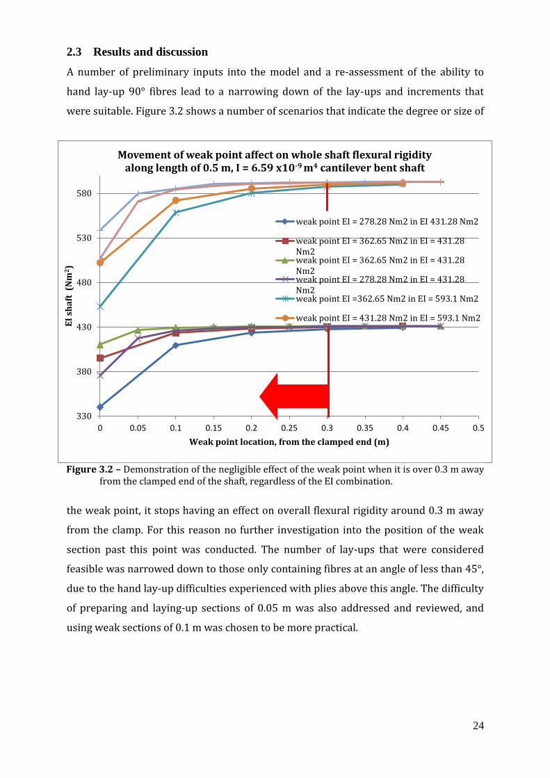
A number of preliminary inputs into the model and a re-assessment of the ability to
hand lay-up 90° fibres lead to a narrowing down of the lay-ups and increments that
were suitable. Figure 3.2 shows a number of scenarios that indicate the degree or size of
the weak point, it stops having an effect on overall flexural rigidity around 0.3 m away
from the clamp. For this reason no further investigation into the position of the weak
section past this point was conducted. The number of lay-ups that were considered
feasible was narrowed down to those only containing fibres at an angle of less than 45°,
due to the hand lay-up difficulties experienced with plies above this angle. The difficulty
of preparing and laying-up sections of 0.05 m was also addressed and reviewed, and
using weak sections of 0.1 m was chosen to be more practical.
330
380
430
480
530
580
0 0.05 0.1 0.15 0.2 0.25 0.3 0.35 0.4 0.45 0.5
EI
sha
ft (
Nm
2)
Weak point location, from the clamped end (m)
Movement of weak point affect on whole shaft flexural rigidity along length of 0.5 m, I = 6.59 x10⁻⁹ m4 cantilever bent shaft
weak point EI = 278.28 Nm2 in EI 431.28 Nm2
weak point EI = 362.65 Nm2 in EI = 431.28Nm2weak point EI = 362.65 Nm2 in EI = 431.28Nm2weak point EI = 278.28 Nm2 in EI = 431.28Nm2weak point EI =362.65 Nm2 in EI = 593.1 Nm2
weak point EI = 431.28 Nm2 in EI = 593.1 Nm2
Figure 3.2 – Demonstration of the negligible effect of the weak point when it is over 0.3 m away from the clamped end of the shaft, regardless of the EI combination.
25
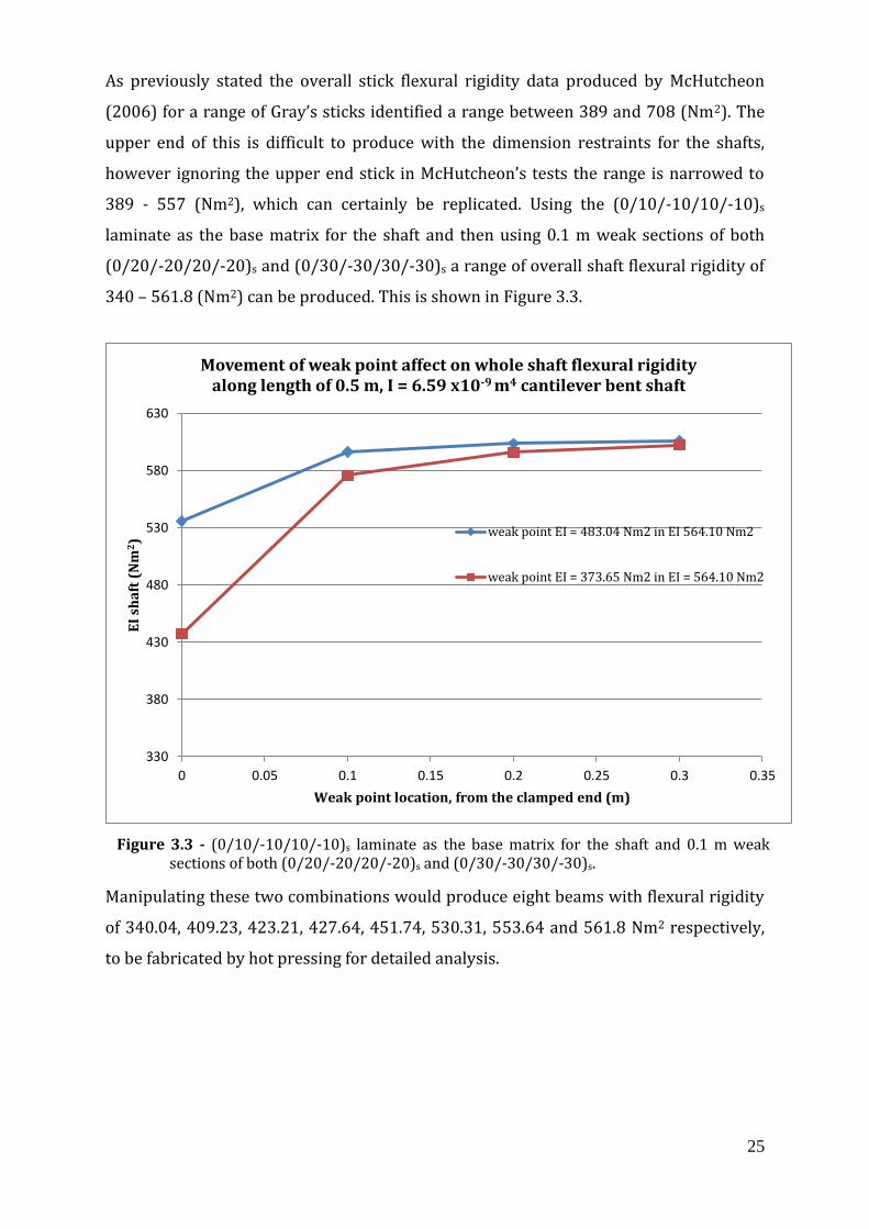
As previously stated the overall stick flexural rigidity data produced by McHutcheon
(2006) for a range of Gray’s sticks identified a range between 389 and 708 (Nm2). The
upper end of this is difficult to produce with the dimension restraints for the shafts,
however ignoring the upper end stick in McHutcheon’s tests the range is narrowed to
389 - 557 (Nm2), which can certainly be replicated. Using the (0/10/-10/10/-10)s
laminate as the base matrix for the shaft and then using 0.1 m weak sections of both
(0/20/-20/20/-20)s and (0/30/-30/30/-30)s a range of overall shaft flexural rigidity of
340 – 561.8 (Nm2) can be produced. This is shown in Figure 3.3.
Manipulating these two combinations would produce eight beams with flexural rigidity
of 340.04, 409.23, 423.21, 427.64, 451.74, 530.31, 553.64 and 561.8 Nm2 respectively,
to be fabricated by hot pressing for detailed analysis.
330
380
430
480
530
580
630
0 0.05 0.1 0.15 0.2 0.25 0.3 0.35
EI
sha
ft (
Nm
2)
Weak point location, from the clamped end (m)
Movement of weak point affect on whole shaft flexural rigidity along length of 0.5 m, I = 6.59 x10⁻⁹ m4 cantilever bent shaft
weak point EI = 483.04 Nm2 in EI 564.10 Nm2
weak point EI = 373.65 Nm2 in EI = 564.10 Nm2
Figure 3.3 - (0/10/-10/10/-10)s laminate as the base matrix for the shaft and 0.1 m weak sections of both (0/20/-20/20/-20)s and (0/30/-30/30/-30)s.
26
3 Preliminary Panel analysis
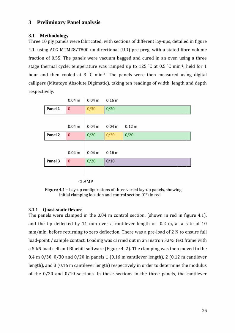
3.1 Methodology Three 10 ply panels were fabricated, with sections of different lay-ups, detailed in figure
4.1, using ACG MTM28/T800 unidirectional (UD) pre-preg. with a stated fibre volume
fraction of 0.55. The panels were vacuum bagged and cured in an oven using a three
stage thermal cycle; temperature was ramped up to 125 ◦C at 0.5 ◦C min-1, held for 1
hour and then cooled at 3 ◦C min-1. The panels were then measured using digital
callipers (Mitutoyo Absolute Digimatic), taking ten readings of width, length and depth
respectively.
0.04 m 0.04 m 0.16 m
Panel 1 0 0/30 0/20
0.04 m 0.04 m 0.04 m 0.12 m
Panel 2 0 0/20 0/30 0/20
0.04 m 0.04 m 0.16 m
Panel 3 0 0/20 0/10
3.1.1 Quasi-static flexure
The panels were clamped in the 0.04 m control section, (shown in red in figure 4.1),
and the tip deflected by 11 mm over a cantilever length of 0.2 m, at a rate of 10
mm/min, before returning to zero deflection. There was a pre-load of 2 N to ensure full
load-point / sample contact. Loading was carried out in an Instron 3345 test frame with
a 5 kN load cell and Bluehill software (Figure 4 .2). The clamping was then moved to the
0.4 m 0/30, 0/30 and 0/20 in panels 1 (0.16 m cantilever length), 2 (0.12 m cantilever
length), and 3 (0.16 m cantilever length) respectively in order to determine the modulus
of the 0/20 and 0/10 sections. In these sections in the three panels, the cantilever
Figure 4.1 – Lay-up configurations of three varied lay-up panels, showing initial clamping location and control section (0°) in red.
CLAMP
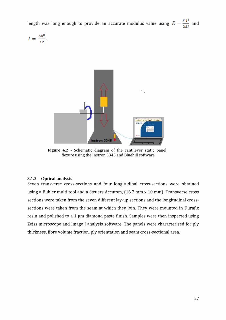
27
length was long enough to provide an accurate modulus value using and
.
3.1.2 Optical analysis
Seven transverse cross-sections and four longitudinal cross-sections were obtained
using a Buhler multi tool and a Struers Accutom, (16.7 mm x 10 mm). Transverse cross
sections were taken from the seven different lay-up sections and the longitudinal cross-
sections were taken from the seam at which they join. They were mounted in Durafix
resin and polished to a 1 µm diamond paste finish. Samples were then inspected using
Zeiss microscope and Image J analysis software. The panels were characterised for ply
thickness, fibre volume fraction, ply orientation and seam cross-sectional area.
Figure 4.2 - Schematic diagram of the cantilever static panel flexure using the Instron 3345 and Bluehill software.
28
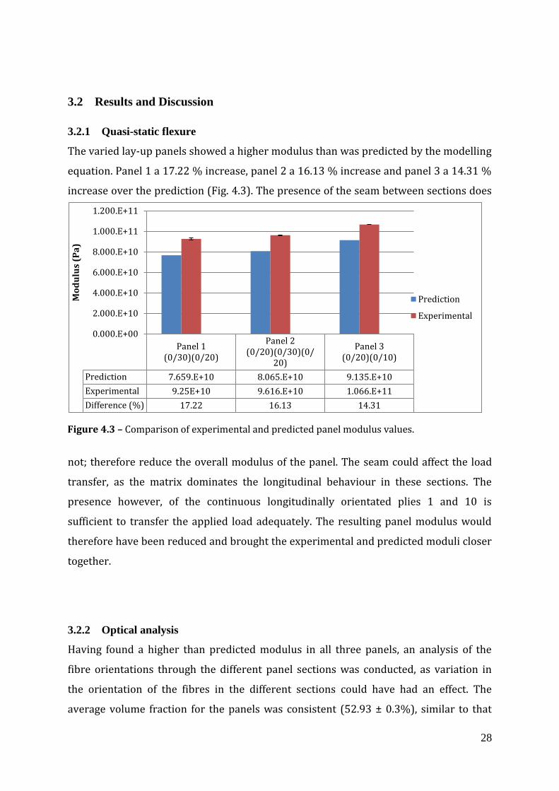
Panel 1(0/30)(0/20)
Panel 2(0/20)(0/30)(0/
20)
Panel 3(0/20)(0/10)
Prediction 7.659.E+10 8.065.E+10 9.135.E+10
Experimental 9.25E+10 9.616.E+10 1.066.E+11
Difference (%) 17.22 16.13 14.31
0.000.E+00
2.000.E+10
4.000.E+10
6.000.E+10
8.000.E+10
1.000.E+11
1.200.E+11
Mo
du
lus
(Pa
)
Prediction
Experimental
3.2 Results and Discussion
3.2.1 Quasi-static flexure
The varied lay-up panels showed a higher modulus than was predicted by the modelling
equation. Panel 1 a 17.22 % increase, panel 2 a 16.13 % increase and panel 3 a 14.31 %
increase over the prediction (Fig. 4.3). The presence of the seam between sections does
not; therefore reduce the overall modulus of the panel. The seam could affect the load
transfer, as the matrix dominates the longitudinal behaviour in these sections. The
presence however, of the continuous longitudinally orientated plies 1 and 10 is
sufficient to transfer the applied load adequately. The resulting panel modulus would
therefore have been reduced and brought the experimental and predicted moduli closer
together.
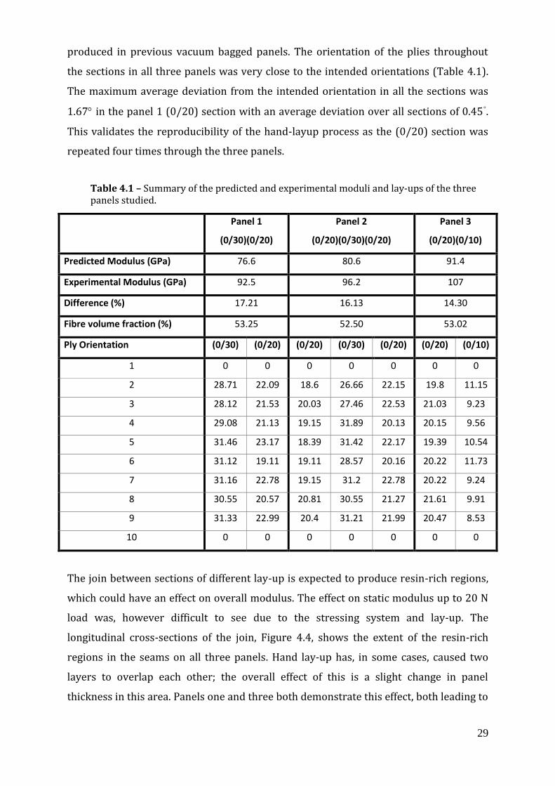
3.2.2 Optical analysis
Having found a higher than predicted modulus in all three panels, an analysis of the
fibre orientations through the different panel sections was conducted, as variation in
the orientation of the fibres in the different sections could have had an effect. The
average volume fraction for the panels was consistent (52.93 ± 0.3%), similar to that
Figure 4.3 – Comparison of experimental and predicted panel modulus values.
29
produced in previous vacuum bagged panels. The orientation of the plies throughout
the sections in all three panels was very close to the intended orientations (Table 4.1).
The maximum average deviation from the intended orientation in all the sections was
1.67 in the panel 1 (0/20) section with an average deviation over all sections of 0.45◦.
This validates the reproducibility of the hand-layup process as the (0/20) section was
repeated four times through the three panels.
Panel 1
(0/30)(0/20)
Panel 2
(0/20)(0/30)(0/20)
Panel 3
(0/20)(0/10)
Predicted Modulus (GPa) 76.6 80.6 91.4
Experimental Modulus (GPa) 92.5 96.2 107
Difference (%) 17.21 16.13 14.30
Fibre volume fraction (%) 53.25 52.50 53.02
Ply Orientation (0/30) (0/20) (0/20) (0/30) (0/20) (0/20) (0/10)
1 0 0 0 0 0 0 0
2 28.71 22.09 18.6 26.66 22.15 19.8 11.15
3 28.12 21.53 20.03 27.46 22.53 21.03 9.23
4 29.08 21.13 19.15 31.89 20.13 20.15 9.56
5 31.46 23.17 18.39 31.42 22.17 19.39 10.54
6 31.12 19.11 19.11 28.57 20.16 20.22 11.73
7 31.16 22.78 19.15 31.2 22.78 20.22 9.24
8 30.55 20.57 20.81 30.55 21.27 21.61 9.91
9 31.33 22.99 20.4 31.21 21.99 20.47 8.53
10 0 0 0 0 0 0 0
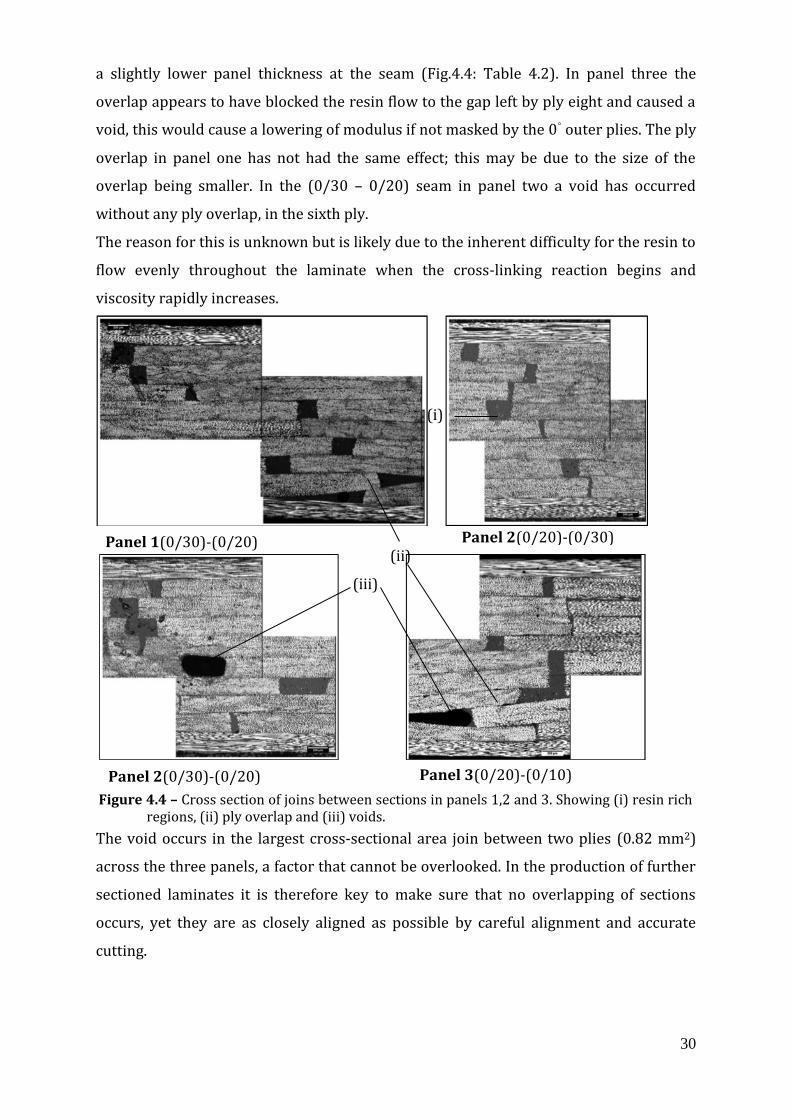
The join between sections of different lay-up is expected to produce resin-rich regions,
which could have an effect on overall modulus. The effect on static modulus up to 20 N
load was, however difficult to see due to the stressing system and lay-up. The
longitudinal cross-sections of the join, Figure 4.4, shows the extent of the resin-rich
regions in the seams on all three panels. Hand lay-up has, in some cases, caused two
layers to overlap each other; the overall effect of this is a slight change in panel
thickness in this area. Panels one and three both demonstrate this effect, both leading to
Table 4.1 – Summary of the predicted and experimental moduli and lay-ups of the three panels studied.
30
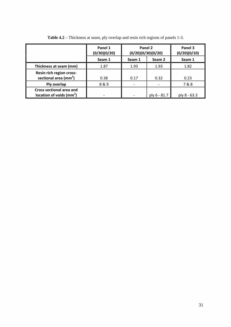
a slightly lower panel thickness at the seam (Fig.4.4: Table 4.2). In panel three the
overlap appears to have blocked the resin flow to the gap left by ply eight and caused a
void, this would cause a lowering of modulus if not masked by the 0◦ outer plies. The ply
overlap in panel one has not had the same effect; this may be due to the size of the
overlap being smaller. In the (0/30 – 0/20) seam in panel two a void has occurred
without any ply overlap, in the sixth ply.
The reason for this is unknown but is likely due to the inherent difficulty for the resin to
flow evenly throughout the laminate when the cross-linking reaction begins and
viscosity rapidly increases.
The void occurs in the largest cross-sectional area join between two plies (0.82 mm2)
across the three panels, a factor that cannot be overlooked. In the production of further
sectioned laminates it is therefore key to make sure that no overlapping of sections
occurs, yet they are as closely aligned as possible by careful alignment and accurate
cutting.
Panel 1(0/30)-(0/20)
(iii)
(ii)
(i)
Panel 2(0/20)-(0/30)
Panel 2(0/30)-(0/20) Panel 3(0/20)-(0/10)
Figure 4.4 – Cross section of joins between sections in panels 1,2 and 3. Showing (i) resin rich regions, (ii) ply overlap and (iii) voids.
31
Table 4.2 – Thickness at seam, ply overlap and resin rich regions of panels 1-3.
Panel 1 (0/30)(0/20)
Panel 2 (0/20)(0/30)(0/20)
Panel 3 (0/20)(0/10)
Seam 1 Seam 1 Seam 2 Seam 1
Thickness at seam (mm) 1.87 1.93 1.93 1.82
Resin rich region cross-sectional area (mm2) 0.38 0.17 0.32 0.23
Ply overlap 8 & 9 - - 7 & 8 Cross sectional area and location of voids (mm2) - - ply 6 - 81.7 ply 8 - 63.3
32
4 Control shafts
4.1 Methodology
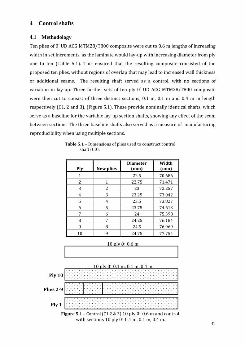
Ten plies of 0◦ UD ACG MTM28/T800 composite were cut to 0.6 m lengths of increasing
width in set increments, as the laminate would lay-up with increasing diameter from ply
one to ten (Table 5.1). This ensured that the resulting composite consisted of the
proposed ten plies, without regions of overlap that may lead to increased wall thickness
or additional seams. The resulting shaft served as a control, with no sections of
variation in lay-up. Three further sets of ten ply 0◦ UD ACG MTM28/T800 composite
were then cut to consist of three distinct sections, 0.1 m, 0.1 m and 0.4 m in length
respectively (C1, 2 and 3), (Figure 5.1). These provide nominally identical shafts, which
serve as a baseline for the variable lay-up section shafts, showing any effect of the seam
between sections. The three baseline shafts also served as a measure of manufacturing
reproducibility when using multiple sections.
Ply New plies Diameter
(mm) Width (mm)
1 22.5 70.686
2 1 22.75 71.471
3 2 23 72.257
4 3 23.25 73.042
5 4 23.5 73.827
6 5 23.75 74.613
7 6 24 75.398
8 7 24.25 76.184
9 8 24.5 76.969
10 9 24.75 77.754
10 ply 0◦ 0.6 m
10 ply 0◦ 0.1 m, 0.1 m, 0.4 m
Plies 2-9
Ply 1
Ply 10
Figure 5.1 – Control (C1,2 & 3) 10 ply 0◦ 0.6 m and control with sections 10 ply 0◦ 0.1 m, 0.1 m, 0.4 m.
Table 5.1 – Dimensions of plies used to construct control shaft (C0).
33
4.1.1 Manufacture
4.1.1.1 Hot pressing
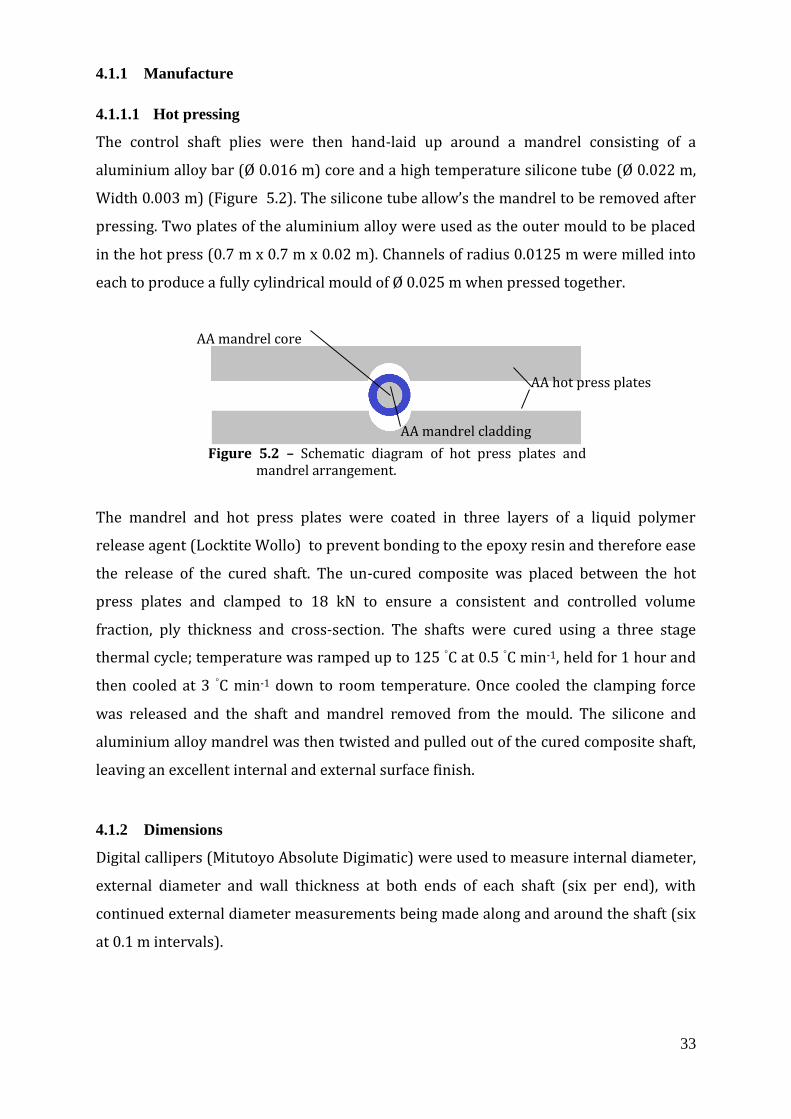
The control shaft plies were then hand-laid up around a mandrel consisting of a
aluminium alloy bar (Ø 0.016 m) core and a high temperature silicone tube (Ø 0.022 m,
Width 0.003 m) (Figure 5.2). The silicone tube allow’s the mandrel to be removed after
pressing. Two plates of the aluminium alloy were used as the outer mould to be placed
in the hot press (0.7 m x 0.7 m x 0.02 m). Channels of radius 0.0125 m were milled into
each to produce a fully cylindrical mould of Ø 0.025 m when pressed together.
The mandrel and hot press plates were coated in three layers of a liquid polymer
release agent (Locktite Wollo) to prevent bonding to the epoxy resin and therefore ease
the release of the cured shaft. The un-cured composite was placed between the hot
press plates and clamped to 18 kN to ensure a consistent and controlled volume
fraction, ply thickness and cross-section. The shafts were cured using a three stage
thermal cycle; temperature was ramped up to 125 ◦C at 0.5 ◦C min-1, held for 1 hour and
then cooled at 3 ◦C min-1 down to room temperature. Once cooled the clamping force
was released and the shaft and mandrel removed from the mould. The silicone and
aluminium alloy mandrel was then twisted and pulled out of the cured composite shaft,
leaving an excellent internal and external surface finish.
4.1.2 Dimensions
Digital callipers (Mitutoyo Absolute Digimatic) were used to measure internal diameter,
external diameter and wall thickness at both ends of each shaft (six per end), with
continued external diameter measurements being made along and around the shaft (six
at 0.1 m intervals).
AA mandrel core
AA mandrel cladding
AA hot press plates
Figure 5.2 – Schematic diagram of hot press plates and mandrel arrangement.
34
4.1.3 Optical analysis
One end transverse section, obtained using a Buhler multi tool and a Struers Accutom
was taken from the 0.6 m control shaft. Mounted in Durafix resin and polished to a 1 µm
diamond paste finish. Samples were then inspected using a Zeiss microscope and Image
J analysis software. The shaft was characterised for ply thickness, fibre volume fraction
and overall wall thickness.
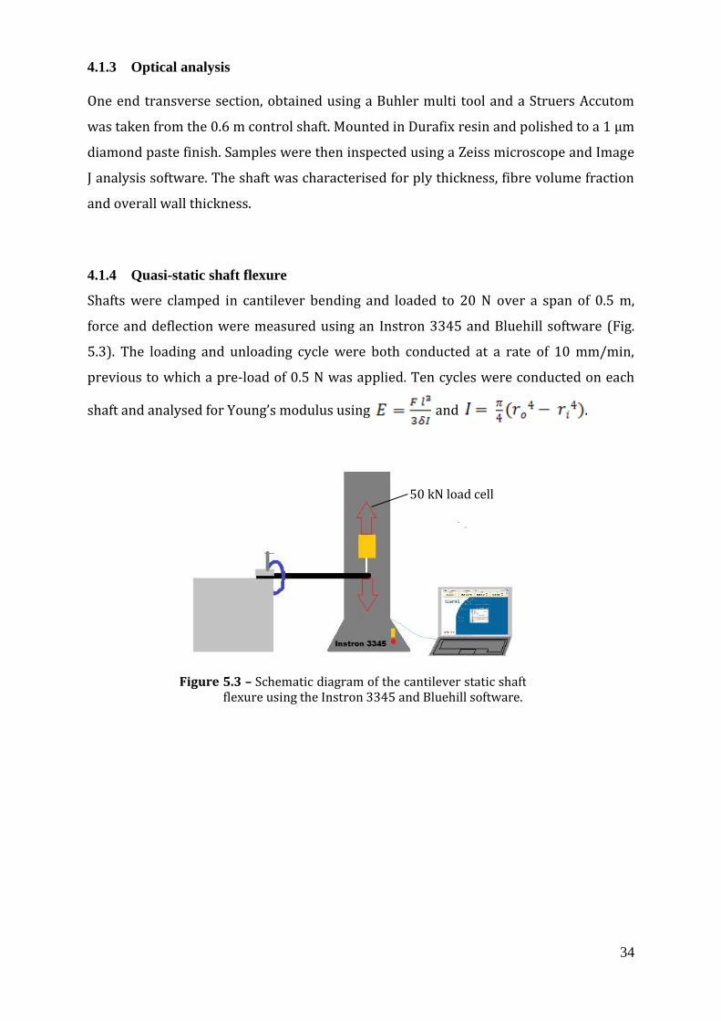
4.1.4 Quasi-static shaft flexure
Shafts were clamped in cantilever bending and loaded to 20 N over a span of 0.5 m,
force and deflection were measured using an Instron 3345 and Bluehill software (Fig.
5.3). The loading and unloading cycle were both conducted at a rate of 10 mm/min,
previous to which a pre-load of 0.5 N was applied. Ten cycles were conducted on each
shaft and analysed for Young’s modulus using and .
Figure 5.3 – Schematic diagram of the cantilever static shaft flexure using the Instron 3345 and Bluehill software.
50 kN load cell
35
23.5
24
24.5
25
25.5
26
26.5
0 0.1 0.2 0.3 0.4 0.5
Dia
me
ter
(mm
)
Distance from clamped end (m)
0
0 section 1
0 section 2
0 section 3
4.2 Results and Discussion
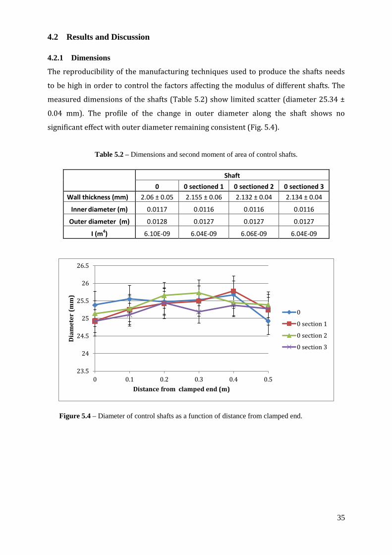
4.2.1 Dimensions
The reproducibility of the manufacturing techniques used to produce the shafts needs
to be high in order to control the factors affecting the modulus of different shafts. The
measured dimensions of the shafts (Table 5.2) show limited scatter (diameter 25.34 ±
0.04 mm). The profile of the change in outer diameter along the shaft shows no
significant effect with outer diameter remaining consistent (Fig. 5.4).
Table 5.2 – Dimensions and second moment of area of control shafts.
Shaft
0 0 sectioned 1 0 sectioned 2 0 sectioned 3
Wall thickness (mm) 2.06 ± 0.05 2.155 ± 0.06 2.132 ± 0.04 2.134 ± 0.04
Inner diameter (m) 0.0117 0.0116 0.0116 0.0116
Outer diameter (m) 0.0128 0.0127 0.0127 0.0127
I (m4) 6.10E-09 6.04E-09 6.06E-09 6.04E-09
Figure 5.4 – Diameter of control shafts as a function of distance from clamped end.
36
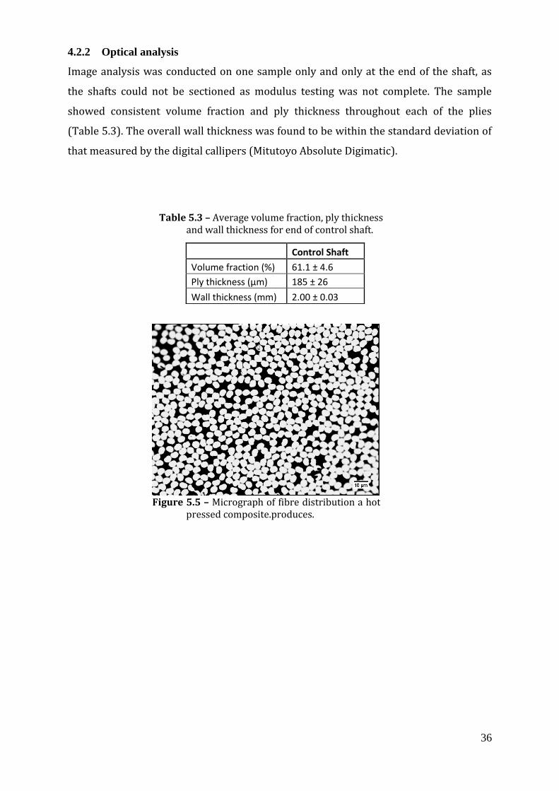
4.2.2 Optical analysis
Image analysis was conducted on one sample only and only at the end of the shaft, as
the shafts could not be sectioned as modulus testing was not complete. The sample
showed consistent volume fraction and ply thickness throughout each of the plies
(Table 5.3). The overall wall thickness was found to be within the standard deviation of
that measured by the digital callipers (Mitutoyo Absolute Digimatic).
Control Shaft
Volume fraction (%) 61.1 ± 4.6
Ply thickness (µm) 185 ± 26
Wall thickness (mm) 2.00 ± 0.03
Figure 5.5 – Micrograph of fibre distribution a hot pressed composite.produces.
Table 5.3 – Average volume fraction, ply thickness and wall thickness for end of control shaft.

37
0.00E+00
2.00E+10
4.00E+10
6.00E+10
8.00E+10
1.00E+11
1.20E+11
Control Sectioned 1 Sectioned 2 Sectioned 3
Mo
du
lus
(Pa
)
Shaft
No-seam (Pa)
Seam (Pa)
Prediction (Pa)
Figure 5.6 – Modulus of control and sectioned shafts in sections with and without seam compared to the CoDA prediction of modulus.
4.2.3 Quasi-static shaft flexure
The nominally identical shafts that had seams in two sections in plies 2 -8 showed
consistent static bend behaviour. The three sectioned shafts in fact showed a higher
average modulus than the control shaft (92.6 GPa and 81.1 GPa respectively). This is not
a significant effect as figure 5.6 shows, the control shafts modulus was contained within
the standard deviation of the sectioned shafts. It is important to note that the prediction
of the modulus of the shafts from previous panel testing input into CoDA (97.3 GPa) was
also within the standard deviation of the sectioned shafts tested. The most important
outcome of the static bend testing was therefore that the seam evident between the
sections has no effect on the static modulus of the shafts, although scatter does increase
with use of multiple sections.

38
5 Multiple section shafts
5.1 Methodology
5.1.1 Manufacture
Five shafts with multiple sections of ten ply UD ACG MTM28/T800 composite were cut
to relevant orientations and lengths (Figure 6.1). Each ply increased in width in set
increments, as the laminate would lay-up with increasing diameter from ply one to ten
(Table 6.1). This ensured that the resulting composite consisted of the proposed ten
plies, without regions of overlap that may lead to increased wall thickness or additional
seams. Figure 6.2 shows an example of how the multiple section shafts were laid-up
with continuous 0◦ fibres in plies 1 and 10 and off axis plies of each section between
them.
Distance along shaft (m)
Shaft 0.1 0.2 0.3 0.4 0.5
V 1 0 0/30 0/20
V 2 0 0/20 0/30 0/20
V 3 0 0/20 0/10
V 4 0 0/10 0/30 0/10
V 5 0 0/10 0/20 0/10
CLAMP Lower EI section
Figure 6.1 – Multiple section shaft’s V 1-5, showing lower EI section placement and overall lay up of shaft.
Table 6.1 – Dimensions of plies used to construct multiple section shaft’s (V 1-5).
Ply New plies Diameter
(mm) Width (mm)
1 22.5 70.69
2 1 22.75 71.47
3 2 23 72.26
4 3 23.25 73.04
5 4 23.5 73.83
6 5 23.75 74.61
7 6 24 75.40
8 7 24.25 76.18
9 8 24.5 76.97
10 9 24.75 77.75
39
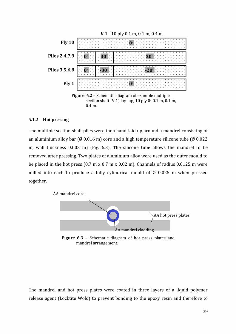
5.1.2 Hot pressing
The multiple section shaft plies were then hand-laid up around a mandrel consisting of
an aluminium alloy bar (Ø 0.016 m) core and a high temperature silicone tube (Ø 0.022
m, wall thickness 0.003 m) (Fig. 6.3). The silicone tube allows the mandrel to be
removed after pressing. Two plates of aluminium alloy were used as the outer mould to
be placed in the hot press (0.7 m x 0.7 m x 0.02 m). Channels of radius 0.0125 m were
milled into each to produce a fully cylindrical mould of Ø 0.025 m when pressed
together.
The mandrel and hot press plates were coated in three layers of a liquid polymer
release agent (Locktite Wolo) to prevent bonding to the epoxy resin and therefore to
Figure 6.2 – Schematic diagram of example multiple section shaft (V 1) lay- up, 10 ply 0◦ 0.1 m, 0.1 m, 0.4 m.
-30◦
0◦
0◦
0◦
30◦ 20◦
0◦
-20◦
V 1 - 10 ply 0.1 m, 0.1 m, 0.4 m
Plies 2,4,7,9
Plies 3,5,6,8
Ply 10
Ply 1
AA mandrel core
AA mandrel cladding
AA hot press plates
Figure 6.3 – Schematic diagram of hot press plates and mandrel arrangement.

40
ease the release of the cured shaft. The un-cured composite was placed between the hot
press plates and clamped to 20 kN to ensure a consistent and controlled volume
fraction, ply thickness and cross-section. The shafts were cured using a three stage
thermal cycle; temperature was ramped up to 125 ◦C at 0.5 ◦C min-1, held for 1 hour and
then cooled at 3 ◦C min-1 down to room temperature. The temperature cycle for shaft V2
was monitored using a thermocouple (RS-1315) attached to the heated platens to verify
the curing cycle (Fig. 6.4). The cycle showed good replication of the thermal cycle used
for vacuum bagged composite production.
Figure 6.4 – Temperature vs. time for curing cycle of shaft V 2 in hot press.
Once cooled the clamping force was released and the shaft and mandrel removed from
the mould. The silicone and aluminium alloy mandrel were then twisted and pulled out
of the cured composite shaft, leaving an excellent internal and external surface finish.
5.1.3 Dimensions
Digital callipers (Mitutoyo Absolute Digimatic) were used to measure internal diameter,
external diameter and wall thickness at both ends of each shaft (six per end), with
continued external diameter measurements being made along and around the shaft (six
at 0.1 m intervals). Once the shafts had been full characterised statically and
dynamically they were sectioned at 0.1 m increments in order to create a wall thickness
profile and a more accurate second moment of area value.
0
20
40
60
80
100
120
0 5 10 15 20 25
Te
mp
(◦C
)
Time (hours)
V 2 hot press cycle

41
5.1.4 Quasi-static shaft flexure
Shafts were clamped in cantilever bending and loaded to 20 N over a span of 0.5 m, and
then decreasing increments of 0.1 m from the clamp. Force-deflection data at 0.2, 0.3,
0.4 and 0.5 m from the clamp were measured using an Instron 3345 and Bluehill
software (Fig. 6.5). The loading and unloading cycle were both conducted at a rate of 10
mm/min, previous to which a pre-load of 2 N was applied. Ten cycles were conducted at
each point on each shaft and analysed for Young’s modulus using and
and deflection profile by the maximum deflection under a load of
20 N at each point. Initially, the effect of the presence and position of the lower EI
section on the static deflection profile was investigated.
Figure 6.5 – Schematic diagram of the cantilever static shaft
flexure using the Instron 3345 and Bluehill software.
5 kN load cell
42
5.1.5 Dynamic drop-ball shaft flexure
To analyse the dynamic behaviour of the multiple sectioned shafts, they were clamped
in a cantilever bend (0.5 m) identical to the quasi-static testing. Clear white markings
were placed at 0.1, 0.2, 0.3, 0.4 and 0.5 m away from the clamped end so to produce
distinct points for the Phantom V7.3 high speed camera and Phantom camera control
software to identify. A Mercian Spider Dimple hockey ball (0.16 kg) was used to impact
the shafts vertically from a range of heights, and therefore impact force (Fig. 6.6). The
resulting shaft deflection was recorded at 6600 fps and then analysed using a
combination of Tracker and Phantom software. Each shaft was evaluated for maximum
deflection at 0.1 m increments along the shaft, impact force and therefore stiffness,
flexural rigidity and modulus and finally CoR. Impact force was determined by the
negative acceleration of the ball from initial contact with the shaft to maximum
deflection using: a = (v – u) / t and F= ma where;
a = acceleration (ms-2)
v = final velocity at maximum deflection
i.e. Rest (ms-1)
u = impact velocity (ms-1)
t = time from impact to maximum
deflection (s)
F = force (N)
M = mass of hockey ball (kg)
43
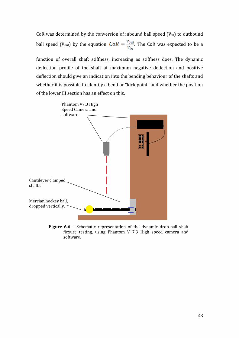
CoR was determined by the conversion of inbound ball speed (Vin) to outbound
ball speed (Vout) by the equation . The CoR was expected to be a
function of overall shaft stiffness, increasing as stiffness does. The dynamic
deflection profile of the shaft at maximum negative deflection and positive
deflection should give an indication into the bending behaviour of the shafts and
whether it is possible to identify a bend or “kick point” and whether the position
of the lower EI section has an effect on this.
Figure 6.6 – Schematic representation of the dynamic drop-ball shaft flexure testing, using Phantom V 7.3 High speed camera and software.
Phantom V7.3 High Speed Camera and software
Cantilever clamped shafts. Mercian hockey ball, dropped vertically.
44
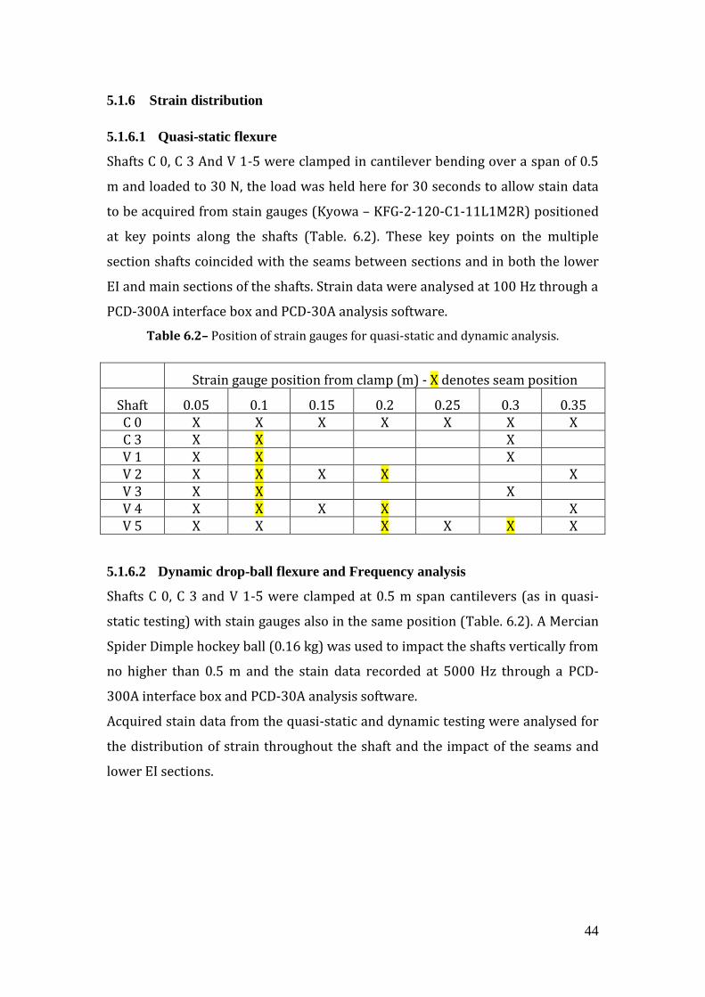
5.1.6 Strain distribution
5.1.6.1 Quasi-static flexure
Shafts C 0, C 3 And V 1-5 were clamped in cantilever bending over a span of 0.5
m and loaded to 30 N, the load was held here for 30 seconds to allow stain data
to be acquired from stain gauges (Kyowa – KFG-2-120-C1-11L1M2R) positioned
at key points along the shafts (Table. 6.2). These key points on the multiple
section shafts coincided with the seams between sections and in both the lower
EI and main sections of the shafts. Strain data were analysed at 100 Hz through a
PCD-300A interface box and PCD-30A analysis software.
Table 6.2– Position of strain gauges for quasi-static and dynamic analysis.
Strain gauge position from clamp (m) - X denotes seam position
Shaft 0.05 0.1 0.15 0.2 0.25 0.3 0.35 C 0 X X X X X X X C 3 X X X V 1 X X X V 2 X X X X X V 3 X X X V 4 X X X X X V 5 X X X X X X
5.1.6.2 Dynamic drop-ball flexure and Frequency analysis
Shafts C 0, C 3 and V 1-5 were clamped at 0.5 m span cantilevers (as in quasi-
static testing) with stain gauges also in the same position (Table. 6.2). A Mercian
Spider Dimple hockey ball (0.16 kg) was used to impact the shafts vertically from
no higher than 0.5 m and the stain data recorded at 5000 Hz through a PCD-
300A interface box and PCD-30A analysis software.
Acquired stain data from the quasi-static and dynamic testing were analysed for
the distribution of strain throughout the shaft and the impact of the seams and
lower EI sections.
45
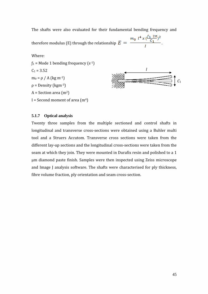
The shafts were also evaluated for their fundamental bending frequency and
therefore modulus (E) through the relationship .
Where:
ƒ1 = Mode 1 bending frequency (s-1)
C1 = 3.52
m0 = ρ / A (kg m-1)
ρ = Density (kgm-3)
A = Section area (m2)
I = Second moment of area (m4)
5.1.7 Optical analysis
Twenty three samples from the multiple sectioned and control shafts in
longitudinal and transverse cross-sections were obtained using a Buhler multi
tool and a Struers Accutom. Transverse cross sections were taken from the
different lay-up sections and the longitudinal cross-sections were taken from the
seam at which they join. They were mounted in Durafix resin and polished to a 1
µm diamond paste finish. Samples were then inspected using Zeiss microscope
and Image J analysis software. The shafts were characterised for ply thickness,
fibre volume fraction, ply orientation and seam cross-section.
l
C1

46
5.2 Results and Discussion
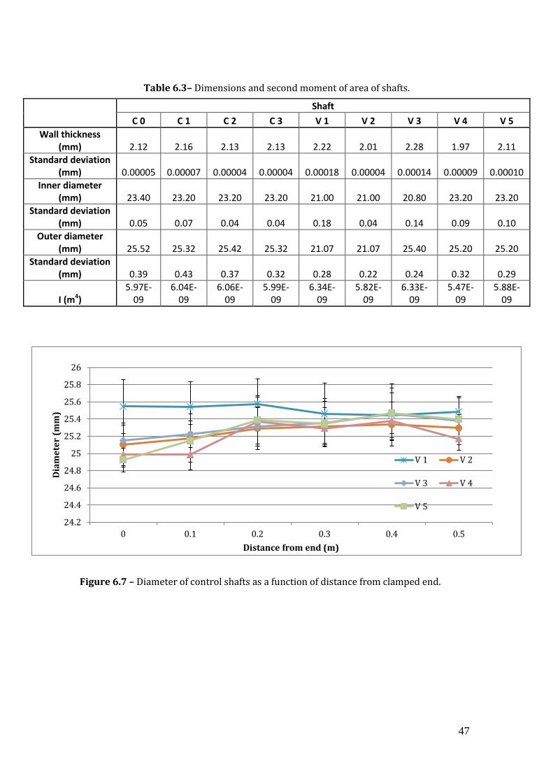
5.2.1 Dimensions
The reproducibility of the manufacturing techniques used to produce the shafts
needs to be high in order to control the factors affecting the modulus of different
shafts. The measured dimensions of the shafts (Table 6.3) show limited scatter
(diameter 25.30 ± 0.02 mm). The profile of the change in outer diameter along
the shaft shows a slight increase in diameter towards the centre in all but shaft V
1. V 1 was cured under a lower load than shafts V 2, V 4 and V 5, this was due to a
fault in the hot press. The effect of this only appears to be at lengths between 0
and 0.3 m where average diameter is up to 0.4 mm larger than shafts V 2 – V 5.
An explanation for this could be that due to the hot press fault, there was uneven
loading on this shaft, not consolidating the plies in this region and could lead to a
lower volume fraction; this will be investigated through optical microscopy.
Taking this into account the scatter between shafts V2 –V5 is low and diameter
profile follows a similar trend (Fig. 6.7). There was also a fault on the hot press
during the production of shaft V 3 which led to its higher wall thickness and
second moment of area values. The distribution of the increased diameter,
however, is different to that of shaft V 1 in that it shows the totally opposite
diameter profile.
The wall thickness values obtained from both ends of the shafts are significantly
higher than those used to model the behaviour of the shafts. The average wall
thickness produced from shafts in the hot press is 2.13 ± 0.08 mm whereas the
wall thickness used in the modelling stage, derived from given single ply
thickness values of the MTM28/High Strength-T800 carbon fibre composite was
1.25 mm. The average ply thickness obtained from initial optical microscopy
conducted on shaft C 0 showed an average ply thickness of 185 ± 26 µm, a
significant increase from 125 µm.
47
24.2
24.4
24.6
24.8
25
25.2
25.4
25.6
25.8
26
0 0.1 0.2 0.3 0.4 0.5
Dia
me
ter
(mm
)
Distance from end (m)
V 1 V 2
V 3 V 4
V 5
Shaft
C 0 C 1 C 2 C 3 V 1 V 2 V 3 V 4 V 5
Wall thickness (mm) 2.12 2.16 2.13 2.13 2.22 2.01 2.28 1.97 2.11
Standard deviation (mm) 0.00005 0.00007 0.00004 0.00004 0.00018 0.00004 0.00014 0.00009 0.00010
Inner diameter (mm) 23.40 23.20 23.20 23.20 21.00 21.00 20.80 23.20 23.20
Standard deviation (mm) 0.05 0.07 0.04 0.04 0.18 0.04 0.14 0.09 0.10
Outer diameter (mm) 25.52 25.32 25.42 25.32 21.07 21.07 25.40 25.20 25.20
Standard deviation (mm) 0.39 0.43 0.37 0.32 0.28 0.22 0.24 0.32 0.29
I (m4)
5.97E-09
6.04E-09
6.06E-09
5.99E-09
6.34E-09
5.82E-09
6.33E-09
5.47E-09
5.88E-09
Figure 6.7 – Diameter of control shafts as a function of distance from clamped end.
Table 6.3– Dimensions and second moment of area of shafts.
48
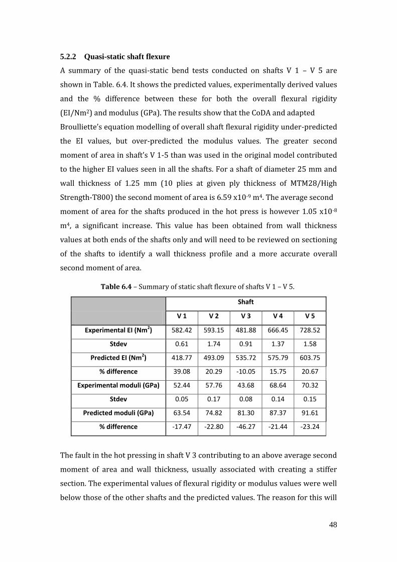
5.2.2 Quasi-static shaft flexure
A summary of the quasi-static bend tests conducted on shafts V 1 – V 5 are
shown in Table. 6.4. It shows the predicted values, experimentally derived values
and the % difference between these for both the overall flexural rigidity
(EI/Nm2) and modulus (GPa). The results show that the CoDA and adapted
Broulliette’s equation modelling of overall shaft flexural rigidity under-predicted
the EI values, but over-predicted the modulus values. The greater second
moment of area in shaft’s V 1-5 than was used in the original model contributed
to the higher EI values seen in all the shafts. For a shaft of diameter 25 mm and
wall thickness of 1.25 mm (10 plies at given ply thickness of MTM28/High
Strength-T800) the second moment of area is 6.59 x10⁻⁹ m4. The average second
moment of area for the shafts produced in the hot press is however 1.05 x10⁻⁸
m4, a significant increase. This value has been obtained from wall thickness
values at both ends of the shafts only and will need to be reviewed on sectioning
of the shafts to identify a wall thickness profile and a more accurate overall
second moment of area.
Shaft
V 1 V 2 V 3 V 4 V 5
Experimental EI (Nm2) 582.42 593.15 481.88 666.45 728.52
Stdev 0.61 1.74 0.91 1.37 1.58
Predicted EI (Nm2) 418.77 493.09 535.72 575.79 603.75
% difference 39.08 20.29 -10.05 15.75 20.67
Experimental moduli (GPa) 52.44 57.76 43.68 68.64 70.32
Stdev 0.05 0.17 0.08 0.14 0.15
Predicted moduli (GPa) 63.54 74.82 81.30 87.37 91.61
% difference -17.47 -22.80 -46.27 -21.44 -23.24
The fault in the hot pressing in shaft V 3 contributing to an above average second
moment of area and wall thickness, usually associated with creating a stiffer
section. The experimental values of flexural rigidity or modulus values were well
below those of the other shafts and the predicted values. The reason for this will
Table 6.4 – Summary of static shaft flexure of shafts V 1 – V 5.
49
0
100
200
300
400
500
600
700
800
V 1 V 2 V 3 V 4 V 5
Shaft
Fle
xu
ral
Rig
idit
y (
Nm
2)
Experimental EI (Nm2)
Predicted EI (Nm2)
0
10
20
30
40
50
60
70
80
90
100
V 1 V 2 V 3 V 4 V 5
Shaft
Mo
du
lus
(G
Pa
)
Experimental moduli (GPa)
Predicted moduli (GPa)
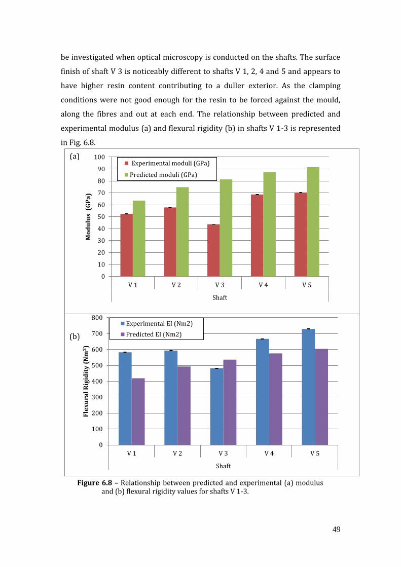
be investigated when optical microscopy is conducted on the shafts. The surface
finish of shaft V 3 is noticeably different to shafts V 1, 2, 4 and 5 and appears to
have higher resin content contributing to a duller exterior. As the clamping
conditions were not good enough for the resin to be forced against the mould,
along the fibres and out at each end. The relationship between predicted and
experimental modulus (a) and flexural rigidity (b) in shafts V 1-3 is represented
in Fig. 6.8.
Figure 6.8 – Relationship between predicted and experimental (a) modulus and (b) flexural rigidity values for shafts V 1-3.
(a)
(a)
(b)
50
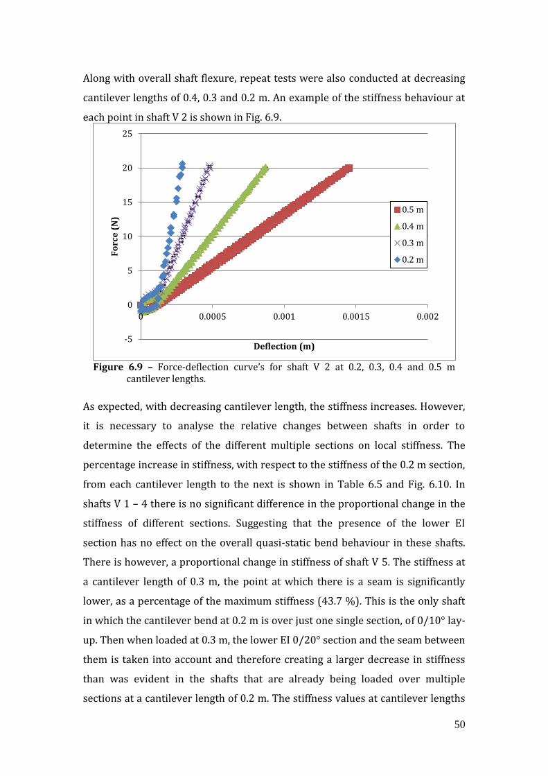
-5
0
5
10
15
20
25
0 0.0005 0.001 0.0015 0.002
Fo
rce
(N
)
Deflection (m)
0.5 m
0.4 m
0.3 m
0.2 m
Along with overall shaft flexure, repeat tests were also conducted at decreasing
cantilever lengths of 0.4, 0.3 and 0.2 m. An example of the stiffness behaviour at
each point in shaft V 2 is shown in Fig. 6.9.
As expected, with decreasing cantilever length, the stiffness increases. However,
it is necessary to analyse the relative changes between shafts in order to
determine the effects of the different multiple sections on local stiffness. The
percentage increase in stiffness, with respect to the stiffness of the 0.2 m section,
from each cantilever length to the next is shown in Table 6.5 and Fig. 6.10. In
shafts V 1 – 4 there is no significant difference in the proportional change in the
stiffness of different sections. Suggesting that the presence of the lower EI
section has no effect on the overall quasi-static bend behaviour in these shafts.
There is however, a proportional change in stiffness of shaft V 5. The stiffness at
a cantilever length of 0.3 m, the point at which there is a seam is significantly
lower, as a percentage of the maximum stiffness (43.7 %). This is the only shaft
in which the cantilever bend at 0.2 m is over just one single section, of 0/10° lay-
up. Then when loaded at 0.3 m, the lower EI 0/20° section and the seam between
them is taken into account and therefore creating a larger decrease in stiffness
than was evident in the shafts that are already being loaded over multiple
sections at a cantilever length of 0.2 m. The stiffness values at cantilever lengths
Figure 6.9 – Force-deflection curve’s for shaft V 2 at 0.2, 0.3, 0.4 and 0.5 m cantilever lengths.

51
0.4 m and 0.5 m are also significantly higher (27.2 and 16.2 %) when compared
to shafts V 1 - 4 (Table 6.5, Fig. 6.10). This could be due to the point at which
bending, or maximum strain is occurring, if the maximum strain point is moved
down the shaft by the lower EI section (between 0.2 and 0.3 m), then this could
have an impact on the effective cantilever length of the shaft. It is expected, in
uniform parallel sided shafts, loaded in cantilever for maximum strain to occur
next to the clamp and therefore controlling the stiffness as the full length of the
shaft is being strained a uniformly decreasing amount. If maximum strain does
not occur next to the clamp then the effective cantilever length is decreased and
therefore increasing the measured stiffness.
Position (m)
0.2 0.3 0.4 0.5
V 1 (N/m) 105586.71 48307.53 24681.25 14406.01
% 100.0 54.2 23.4 13.6
V2 (N/m) 112837.92 52204.69 25871.88 14671.26
% 100.0 53.7 22.9 13.0
V3 (N/m) 89130.87 41882.69 20525.47 11919.11
% 100.0 53.0 23.0 13.4
V4 (N/m) 125467.36 58195.80 27945.86 16484.37
% 100.0 53.6 22.3 13.1
V5 (N/m) 111226.90 62671.38 30229.25 18019.67
% 100.0 43.7 27.2 16.2
Table 6.5 – Percentage decrease in stiffness as cantilever length increases in shafts V 1-5.
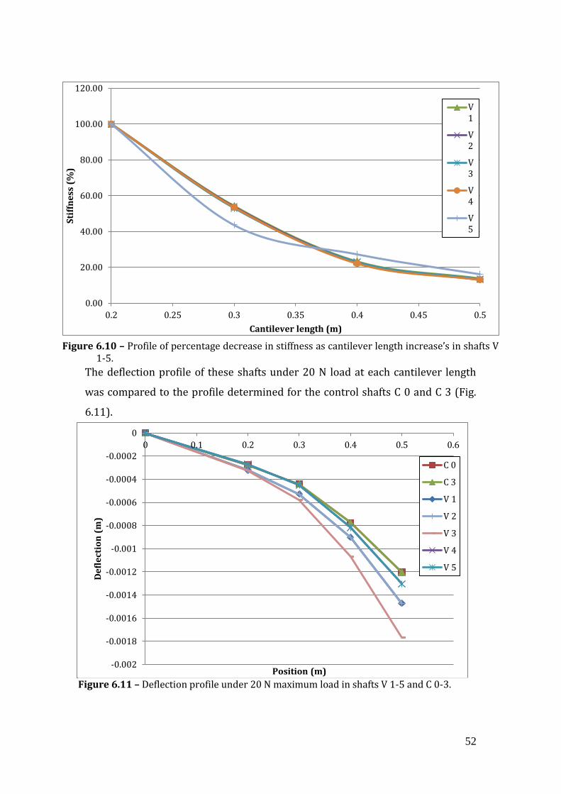
52
0.00
20.00
40.00
60.00
80.00
100.00
120.00
0.2 0.25 0.3 0.35 0.4 0.45 0.5
Sti
ffn
ess
(%
)
Cantilever length (m)
V1
V2
V3
V4
V5
-0.002
-0.0018
-0.0016
-0.0014
-0.0012
-0.001
-0.0008
-0.0006
-0.0004
-0.0002
0
0 0.1 0.2 0.3 0.4 0.5 0.6
De
fle
ctio
n (
m)
Position (m)
C 0
C 3
V 1
V 2
V 3
V 4
V 5
The deflection profile of these shafts under 20 N load at each cantilever length
was compared to the profile determined for the control shafts C 0 and C 3 (Fig.
6.11).
Figure 6.11 – Deflection profile under 20 N maximum load in shafts V 1-5 and C 0-3.
Figure 6.10 – Profile of percentage decrease in stiffness as cantilever length increase’s in shafts V 1-5.

53
The deflection profile of the control shafts C 0 and C 3 shows little scatter, indeed
shafts V 1 and 2 also show an identical profile of maximum deflection under 20 N
load. It is interesting to see that at 0.2 m cantilever bend shafts V 1-3 are very
closely matched; however the lower flexural rigidity and modulus shaft V 3 then
starts to deflect more with respect to V 1 and 2. This suggests that it is at this
point that the shaft strains the most and where bending is controlled from. A
similar effect can be seen in shafts C 0, 3 and V 5. They all show a closely
matched deflection profile up to 0.3 m cantilever length, then at this point shaft V
5 begins to deviate away from the control shafts and deflect a greater amount.
Developing on from the discussed impact of the lower EI section and the seams
in this shaft. Quasi-static testing with strain gauge data will be conducted to
understand this further.

54
-0.10
0.00
0.10
0.20
0.30
0.40
0.50
0.60
0.70
0.00
10.00
20.00
30.00
40.00
50.00
60.00
70.00
80.00
C 0 / V 1 C 3 / V 2 V 3 V 4 V 5
Co
R
E (
Gp
a)
Shaft
E (Gpa) C 0-3 E (Gpa) V 1-5 CoR C 0-3 CoR V 1-5
5.2.3 Dynamic drop-ball shaft flexure
In dynamic testing shafts C 0 -3 and V 1-5 showed a much lower modulus when
compared to quasi-static testing. This could be due to the use of maximum
deflection, but only average applied force. They did however follow similar
trends in terms of the relationship between the shafts. Shaft C 0 showed the
highest modulus from the dynamic testing (65.35 ± 4.13 GPa), followed closely
by C 3 (63.41 ±3.09 GPa). The conversion of this modulus into dynamic ball
interaction gave these shafts a CoR of 0.50 and 0.39 respectively, a concurrent
drop in CoR with the presence of the seam in C 3. The ability of the multi-
sectioned shafts V 1-5 of converting inbound ball speed into outbound ball speed
differed from that of the control shafts. Even though shafts V 1-5 displayed a
lower modulus, they did in fact have a higher CoR than the control shafts in some
cases. There is a good relationship between the modulus of all the multi-
sectioned shafts, as modulus increases so does CoR and vice-versa (Fig. 6.12).
To understand what is happening to the shafts during deflection and subsequent
release of the ball at impact, Tracker software was used to track points at 0.1,
0.2, 0.3, 0.4 and 0.5 m from the clamp. The bending profile of the shaft would
give an indication of the bend point and the extent to which the position of seams
and lower EI sections affects this. The data acquired from Tracker are displayed
Figure 6.12 – Dynamic modulus and CoR values for control and multi-sectioned shafts.

55
-0.018
-0.016
-0.014
-0.012
-0.01
-0.008
-0.006
-0.004
-0.002
0
0.002
0.004
0 0.1 0.2 0.3 0.4 0.5
De
fle
ctio
n (
m)
Position (m)
C 0 -ve
C 1-3 -ve
C 0 +ve
C 1-3 +ve
(a)
-0.020
-0.018
-0.016
-0.014
-0.012
-0.010
-0.008
-0.006
-0.004
-0.002
0.000
0.002
0.004
0.006
0 0.1 0.2 0.3 0.4 0.5
De
fle
ctio
n (
m)
Position (m)
V 1 -veV 2 -veV 3 -veV 4 -veV 5 -veV 1 +veV 2 +veV 3 +veV 4 +veV 5 +ve
(b)
in Fig. 6.13, but it is certainly not conclusive. There does not appear to be a
difference in the deflection profile between the control (a) and multi-sectioned
(b) shafts. Deflection in the negative direction following ball impact and the
subsequent positive deflection at ball release show a high scatter and do not
display any noticeable relationships. For this reason dynamic data will be
acquired using strain gauges at key points along the shafts to fully determine the
dynamic behaviour.
Figure 6.13 – Maximum negative and positive dynamic deflection profile for control (a) and multi-sectioned (b) shafts.
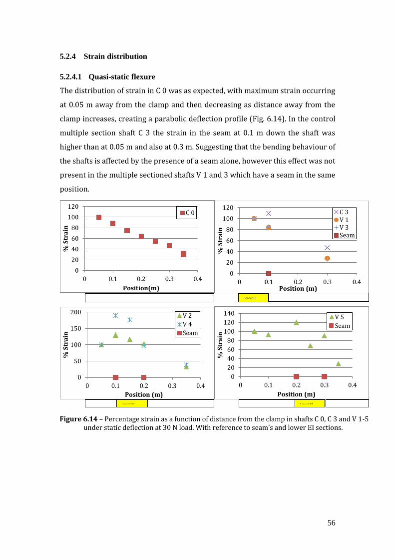
56
0
20
40
60
80
100
120
0 0.1 0.2 0.3 0.4
% S
tra
in
Position (m)
C 3V 1V 3Seam
0
20
40
60
80
100
120
0 0.1 0.2 0.3 0.4
% S
tra
in
Position(m)
C 0
0
50
100
150
200
0 0.1 0.2 0.3 0.4
% S
tra
in
Position (m)
V 2
V 4
Seam
0
20
40
60
80
100
120
140
0 0.1 0.2 0.3 0.4
% S
tra
in
Position (m)
V 5
Seam
5.2.4 Strain distribution
5.2.4.1 Quasi-static flexure
The distribution of strain in C 0 was as expected, with maximum strain occurring
at 0.05 m away from the clamp and then decreasing as distance away from the
clamp increases, creating a parabolic deflection profile (Fig. 6.14). In the control
multiple section shaft C 3 the strain in the seam at 0.1 m down the shaft was
higher than at 0.05 m and also at 0.3 m. Suggesting that the bending behaviour of
the shafts is affected by the presence of a seam alone, however this effect was not
present in the multiple sectioned shafts V 1 and 3 which have a seam in the same
position.
Lower EI
Lower EI Lower EI
Figure 6.14 – Percentage strain as a function of distance from the clamp in shafts C 0, C 3 and V 1-5 under static deflection at 30 N load. With reference to seam’s and lower EI sections.
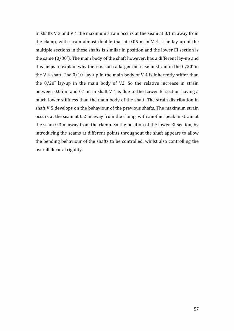
57
In shafts V 2 and V 4 the maximum strain occurs at the seam at 0.1 m away from
the clamp, with strain almost double that at 0.05 m in V 4. The lay-up of the
multiple sections in these shafts is similar in position and the lower EI section is
the same (0/30˚). The main body of the shaft however, has a different lay-up and
this helps to explain why there is such a larger increase in strain in the 0/30˚ in
the V 4 shaft. The 0/10˚ lay-up in the main body of V 4 is inherently stiffer than
the 0/20˚ lay-up in the main body of V2. So the relative increase in strain
between 0.05 m and 0.1 m in shaft V 4 is due to the Lower EI section having a
much lower stiffness than the main body of the shaft. The strain distribution in
shaft V 5 develops on the behaviour of the previous shafts. The maximum strain
occurs at the seam at 0.2 m away from the clamp, with another peak in strain at
the seam 0.3 m away from the clamp. So the position of the lower EI section, by
introducing the seams at different points throughout the shaft appears to allow
the bending behaviour of the shafts to be controlled, whilst also controlling the
overall flexural rigidity.

58
0
20
40
60
80
100
120
0 0.1 0.2 0.3 0.4
% S
tra
in
Position (m)
Seam
C 3
V 1
V 3
0
20
40
60
80
100
120
140
0 0.1 0.2 0.3 0.4
% S
tra
in
Position (m)
Seam
V 5
0
50
100
150
200
0 0.1 0.2 0.3 0.4
% S
tra
in
Position (m)
Seam
V 2
V 4
0
20
40
60
80
100
120
0 0.1 0.2 0.3 0.4
% S
tra
in
Position(m)
C 0
5.2.4.2 Dynamic drop-ball flexure
The shafts behaved very similar dynamically to their static strain distribution.
Following the trends of maximum strain points in the multiple sectioned shafts,
on the seams between sections and decreasing from the clamp in shaft C 0 (Fig.
6.15). There was not as large a difference between the strain behaviour of shafts
V 2 and 4 when tested dynamically. Shaft V 4 did still have a larger increase in
strain from 0.05 m to 0.1 m but the increase was half of that evident in quasi-
static testing
Figure 6.15 – Percentage strain as a function of distance from the clamp in shafts C 0, C 3 and V 1-5 under dynamic deflection. With reference to seam’s and lower EI sections.
Lower EI
Lower EI Lower EI
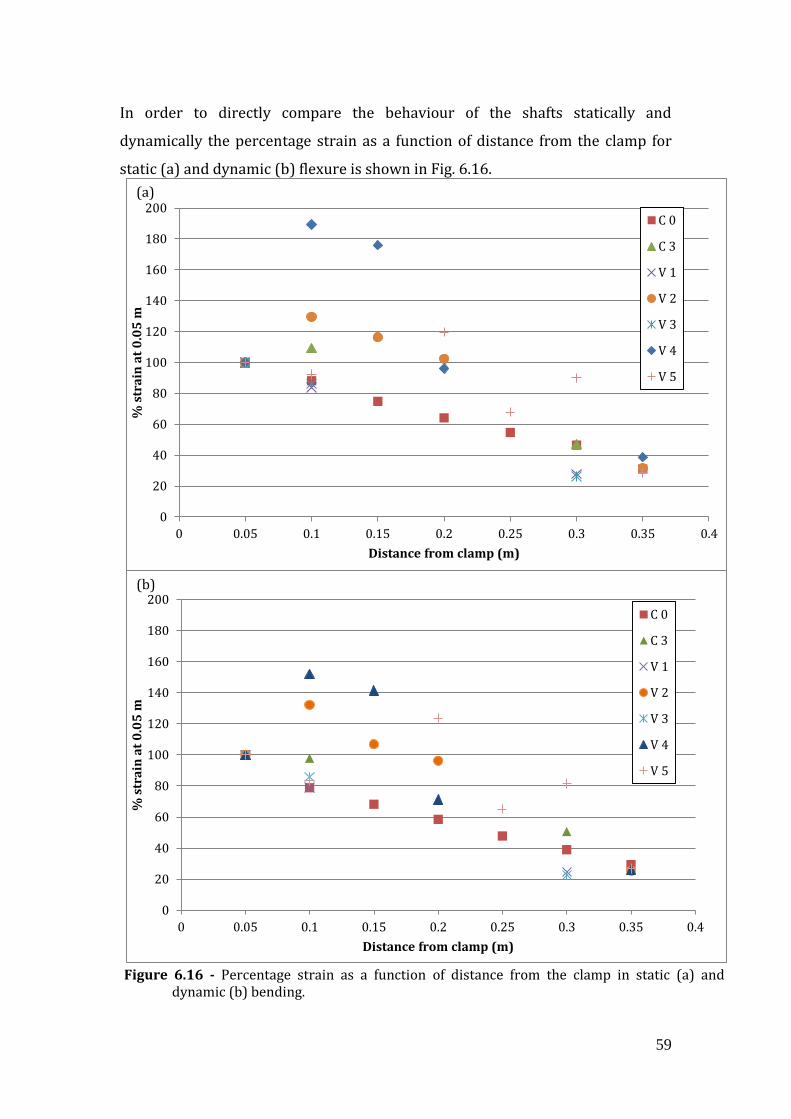
59
0
20
40
60
80
100
120
140
160
180
200
0 0.05 0.1 0.15 0.2 0.25 0.3 0.35 0.4
% s
tra
in a
t 0
.05
m
Distance from clamp (m)
C 0
C 3
V 1
V 2
V 3
V 4
V 5
(b)
0
20
40
60
80
100
120
140
160
180
200
0 0.05 0.1 0.15 0.2 0.25 0.3 0.35 0.4
% s
tra
in a
t 0
.05
m
Distance from clamp (m)
C 0
C 3
V 1
V 2
V 3
V 4
V 5
(a)
Figure 6.16 - Percentage strain as a function of distance from the clamp in static (a) and dynamic (b) bending.
In order to directly compare the behaviour of the shafts statically and
dynamically the percentage strain as a function of distance from the clamp for
static (a) and dynamic (b) flexure is shown in Fig. 6.16.

60
-200
-100
0
100
200
300
400
500
600
700
0 0.02 0.04 0.06 0.08 0.1
Mic
rost
rain
(µ
m/
m)
Time (s)
0.05
0.1
0.15
0.2
0.25
0.3
0.35
-400
-200
0
200
400
600
800
1000
0 0.02 0.04 0.06 0.08 0.1
Mic
rost
rain
(µ
m/m
)
Time (s)
0.05
0.1
0.15
0.2
0.35
5.2.4.3 Frequency analysis
By using the 1st natural mode of vibrating frequency obtained from the strain
gauge data by analysing the period between peaks, the inverse of this being the
frequency (ƒ = 1 / Λ), the respective modulus of the shafts was derived. The
behaviour of the control shaft C 0 (a) and a multiple sectioned shaft V 4 (b) is
show in Fig. 6.17. The difference in the maximum strain between the shafts is
clear to see and the second mode of bending can also be noticed in the data of
strain most predominantly furthest away from the clamp.
(a)
(b)
Figure 6.17 – Microstrain as a function of time for increasing distances away from the clamp, showing first and second bending modes in C 0 (a) and V 4 (b).
61
0
10
20
30
40
50
60
70
80
C 0 C 3 V 1 V 2 V 3 V 4 V 5
Mo
du
lus
(GP
a)
Shaft
Static Dynamic Frequency
The modulus obtained from the shafts through this method was consistently
higher than that derived from the high speed camera and follows those obtained
by static testing closely. Suggesting that the data acquired from the high speed
camera in terms of impact force and deflection conversion to modulus was not
accurate, or reliable enough because of the use of average force and maximum
deflection in the calculations. (Fig. 6.18).
Ignoring shaft V 3, in all methods of testing there is a clear increase in modulus
from shaft V 1-5 as was initially modelled. The reason for the anomaly shown in
the behaviour of shaft V 3 is not known but will be the focus of microstructural
analysis. A discrepancy in the manufacture of the shafts, for example creating an
assymmetrical laminate could perhaps have contributed to its poor performance.
It has the same section construction as V1 and this does not show a behaviour
that was unexpected, in fact these two shaft only have one seam in comparison to
the highest modulus shaft V 5 which has two seams. It is interesting that even
though the multiple section shafts V 1-5 appear to have underperformed in the
dynamic high speed camera tests, however both control shafts, under the same
testing conditions show a much better correlation to the other testing scenarios.
Figure 6.18 – The modulus obtained for shafts C 0, C 3 and V 1-5 by static, dynamic and frequency analysis methods in comparison to CoDA predicted values.

62
5.3 Optical analysis
The ply orientation in shafts V 1-5 is consistent with the intended laminate
configurations (Figure 6.19). The average deviation from the intended
orientations is shown in Table 6.6 and does not diverge greater than 1.1 degree
away from the projected ply angle.
0
10
20
30
40
0 1 2 3 4 5 6 7 8 9 10
Ori
en
tati
on
(d
ge
ree
s)
Ply
V1 section 1 V1 section 2
0
5
10
15
20
25
0 1 2 3 4 5 6 7 8 9 10O
rie
nta
tio
n (
dg
ere
es)
Ply
V3 section 1 V3 section 2
0
10
20
30
40
0 1 2 3 4 5 6 7 8 9 10
Ori
en
tati
on
(d
ge
ree
s)
Ply
V2 section1 V2 section 2 V2 section 3
0
10
20
30
40
0 1 2 3 4 5 6 7 8 9 10
Ori
en
tati
on
(d
ge
ree
s)
Ply
V4 section 1 V4 section 2 V4 section 3
0
5
10
15
20
25
0 1 2 3 4 5 6 7 8 9 10
Ori
en
tati
on
(d
ge
ree
s)
Ply
V5 section 1 V5 section 2 V5 section 3
Figure 6.19 – Ply orientation throughout the multiple sections in shafts V 1-5.
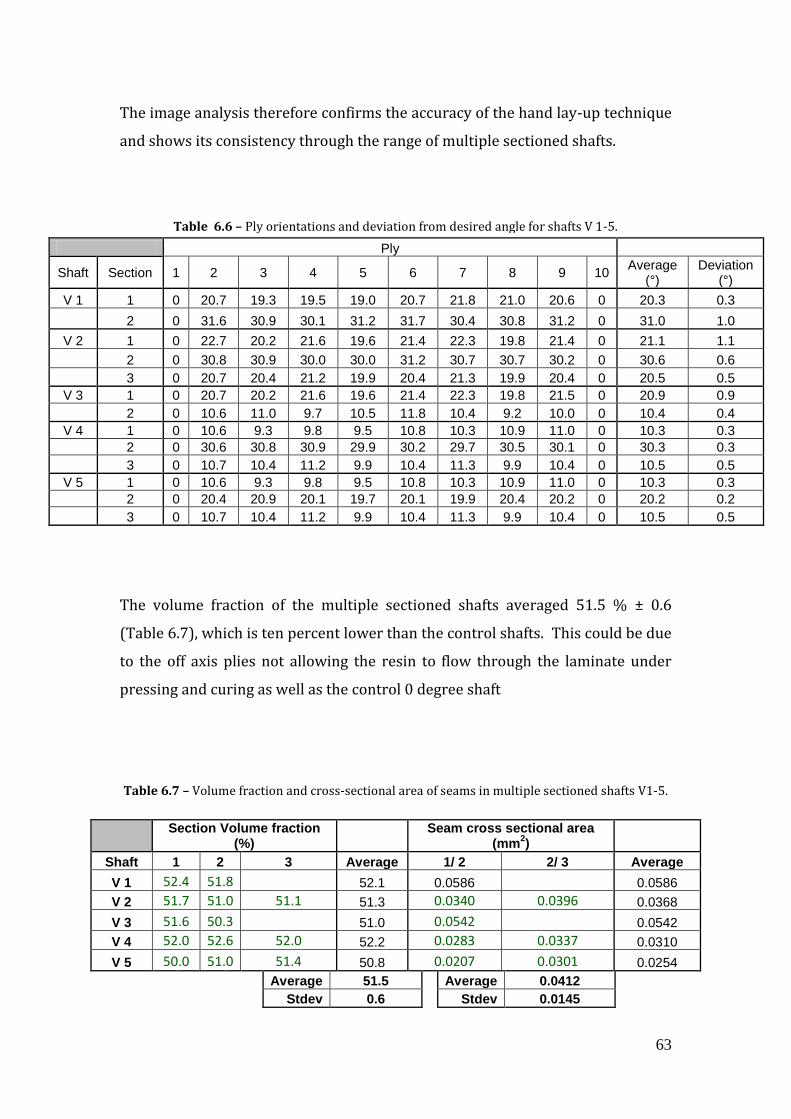
63
The image analysis therefore confirms the accuracy of the hand lay-up technique
and shows its consistency through the range of multiple sectioned shafts.
The volume fraction of the multiple sectioned shafts averaged 51.5 % ± 0.6
(Table 6.7), which is ten percent lower than the control shafts. This could be due
to the off axis plies not allowing the resin to flow through the laminate under
pressing and curing as well as the control 0 degree shaft
Table 6.7 – Volume fraction and cross-sectional area of seams in multiple sectioned shafts V1-5.
Section Volume fraction (%)
Seam cross sectional area (mm
2)
Shaft 1 2 3 Average 1/ 2 2/ 3 Average
V 1 52.4 51.8 52.1 0.0586 0.0586
V 2 51.7 51.0 51.1 51.3 0.0340 0.0396 0.0368
V 3 51.6 50.3 51.0 0.0542 0.0542
V 4 52.0 52.6 52.0 52.2 0.0283 0.0337 0.0310
V 5 50.0 51.0 51.4 50.8 0.0207 0.0301 0.0254
Average 51.5
Average 0.0412
Stdev 0.6
Stdev 0.0145
Ply
Shaft Section 1 2 3 4 5 6 7 8 9 10 Average
(°) Deviation
(°)
V 1 1 0 20.7 19.3 19.5 19.0 20.7 21.8 21.0 20.6 0 20.3 0.3
2 0 31.6 30.9 30.1 31.2 31.7 30.4 30.8 31.2 0 31.0 1.0
V 2 1 0 22.7 20.2 21.6 19.6 21.4 22.3 19.8 21.4 0 21.1 1.1
2 0 30.8 30.9 30.0 30.0 31.2 30.7 30.7 30.2 0 30.6 0.6
3 0 20.7 20.4 21.2 19.9 20.4 21.3 19.9 20.4 0 20.5 0.5
V 3 1 0 20.7 20.2 21.6 19.6 21.4 22.3 19.8 21.5 0 20.9 0.9
2 0 10.6 11.0 9.7 10.5 11.8 10.4 9.2 10.0 0 10.4 0.4
V 4 1 0 10.6 9.3 9.8 9.5 10.8 10.3 10.9 11.0 0 10.3 0.3
2 0 30.6 30.8 30.9 29.9 30.2 29.7 30.5 30.1 0 30.3 0.3
3 0 10.7 10.4 11.2 9.9 10.4 11.3 9.9 10.4 0 10.5 0.5
V 5 1 0 10.6 9.3 9.8 9.5 10.8 10.3 10.9 11.0 0 10.3 0.3
2 0 20.4 20.9 20.1 19.7 20.1 19.9 20.4 20.2 0 20.2 0.2
3 0 10.7 10.4 11.2 9.9 10.4 11.3 9.9 10.4 0 10.5 0.5
Table 6.6 – Ply orientations and deviation from desired angle for shafts V 1-5.

64
Figure 6.20 – Seam V1 0/30-0/20 examples of good ply interaction (i), ply overlap (ii) and also resin rich regions (iii)
Shaft V1 with a 0.1 m 0/30 section and a 0.4 m 0/20 section only has one seam;
the cross-section is shown in Figure 6.20. There are examples of good ply
interaction (i), ply overlap (ii) and also resin rich regions (iii) where the plies are
not flush with one another. This seam showed the highest overall cross-sectional
area of resin rich regions at 0.0586 mm2. This was the first multiple sectioned
shaft to be manufactured with off-axis plies, which added to the complexity of
the hand lay-up process.
Figure 6.21 – Seam 1 V2, 0/20-0/30. Showing the negative effect of ply overlap. resin rich region extending between plies longitudinally.
(iii)
(ii)
(i)
(i)
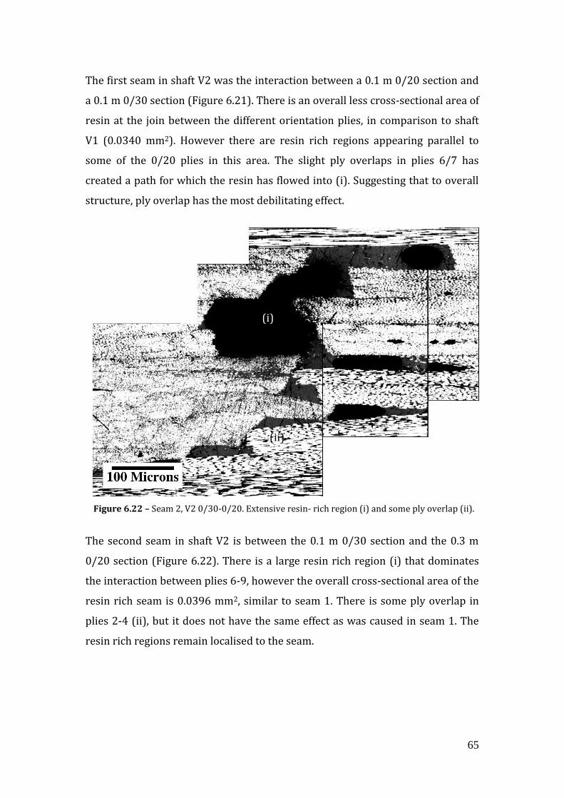
65
Figure 6.22 – Seam 2, V2 0/30-0/20. Extensive resin- rich region (i) and some ply overlap (ii).
The first seam in shaft V2 was the interaction between a 0.1 m 0/20 section and
a 0.1 m 0/30 section (Figure 6.21). There is an overall less cross-sectional area of
resin at the join between the different orientation plies, in comparison to shaft
V1 (0.0340 mm2). However there are resin rich regions appearing parallel to
some of the 0/20 plies in this area. The slight ply overlaps in plies 6/7 has
created a path for which the resin has flowed into (i). Suggesting that to overall
structure, ply overlap has the most debilitating effect.
The second seam in shaft V2 is between the 0.1 m 0/30 section and the 0.3 m
0/20 section (Figure 6.22). There is a large resin rich region (i) that dominates
the interaction between plies 6-9, however the overall cross-sectional area of the
resin rich seam is 0.0396 mm2, similar to seam 1. There is some ply overlap in
plies 2-4 (ii), but it does not have the same effect as was caused in seam 1. The
resin rich regions remain localised to the seam.
(i)
(ii)
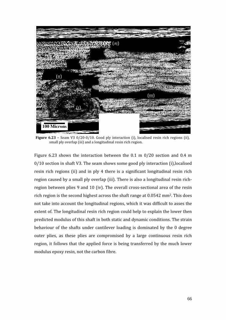
66
Figure 6.23 – Seam V3 0/20-0/10. Good ply interaction (i), localised resin rich regions (ii), small ply overlap (iii) and a longitudinal resin rich region.
Figure 6.23 shows the interaction between the 0.1 m 0/20 section and 0.4 m
0/10 section in shaft V3. The seam shows some good ply interaction (i),localised
resin rich regions (ii) and in ply 4 there is a significant longitudinal resin rich
region caused by a small ply overlap (iii). There is also a longitudinal resin rich-
region between plies 9 and 10 (iv). The overall cross-sectional area of the resin
rich region is the second highest across the shaft range at 0.0542 mm2. This does
not take into account the longitudinal regions, which it was difficult to asses the
extent of. The longitudinal resin rich region could help to explain the lower then
predicted modulus of this shaft in both static and dynamic conditions. The strain
behaviour of the shafts under cantilever loading is dominated by the 0 degree
outer plies, as these plies are compromised by a large continuous resin rich
region, it follows that the applied force is being transferred by the much lower
modulus epoxy resin, not the carbon fibre.
(i)
(ii)
(iii)
(iv)
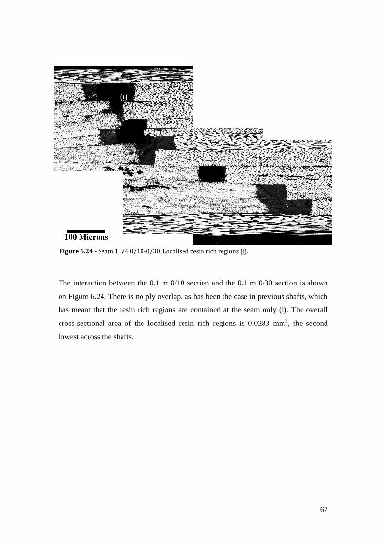
67
The interaction between the 0.1 m 0/10 section and the 0.1 m 0/30 section is shown
on Figure 6.24. There is no ply overlap, as has been the case in previous shafts, which
has meant that the resin rich regions are contained at the seam only (i). The overall
cross-sectional area of the localised resin rich regions is 0.0283 mm2, the second
lowest across the shafts.
Figure 6.24 - Seam 1, V4 0/10-0/30. Localised resin rich regions (i).
(i)

68
The second seam in shaft V4 is between the 0.1 m 0/30 section and 0.2 m 0/10
section. The interaction is dominated by localised resin rich regions (i). There is
also a ply overlap (ii) that has caused a larger resin rich region and some ply
distortion in that area. The overall cross sectional area of the resin rich regions
was 0.0337 mm2.
Figure 6.24 – Seam 2, V4 0/30 – 0/10. Ply overlap (i) and localised resin rich regions (ii).
(i)
(ii)
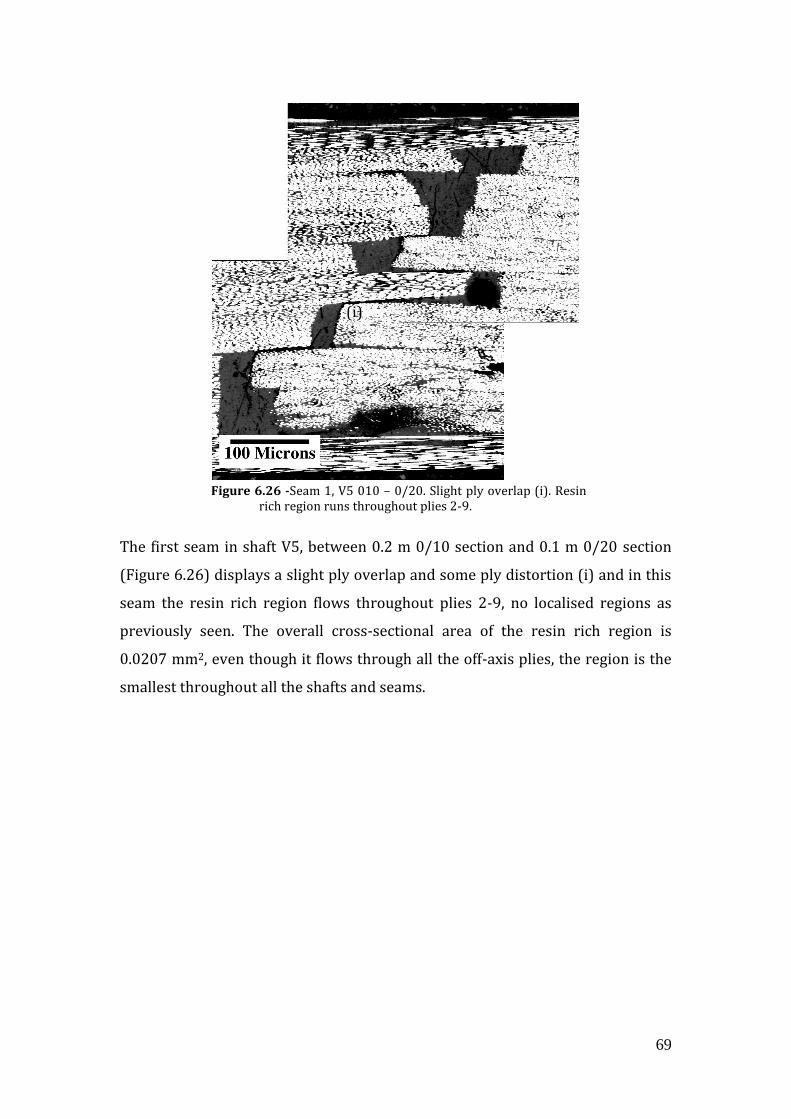
69
The first seam in shaft V5, between 0.2 m 0/10 section and 0.1 m 0/20 section
(Figure 6.26) displays a slight ply overlap and some ply distortion (i) and in this
seam the resin rich region flows throughout plies 2-9, no localised regions as
previously seen. The overall cross-sectional area of the resin rich region is
0.0207 mm2, even though it flows through all the off-axis plies, the region is the
smallest throughout all the shafts and seams.
Figure 6.26 -Seam 1, V5 010 – 0/20. Slight ply overlap (i). Resin rich region runs throughout plies 2-9.
(i)

70
Figure 6.27 – Seam 2,V5 . 0/20 – 0/10. Large resin rich region (i) causes ply distortion throughout the laminate. Localised resin rich regions (ii) and small ply overlap (iii).
The final seam in shaft V5 shown in Figure 6.27, is between the 0.1 m 0/20
section and 0.2 m 0/10. It displays a large resin rich region in plies 2 and 3 which
causes ply distortion that runs throughout the laminate, bowing the plies away
from parallel (i). There is also some localised resin rich regions (ii) and some
small ply overlap contributing to some further slight distortion. The overall
cross-sectional area of the resin rich regions throughout the ply is 0.0307 mm2.
71
6 Conclusions
Using CoDA and the manipulated Broulliette equation to predict the
behaviour of composite shafts with multiple sections gave a good
understanding of the trend of behavior that was to be expected, but was not
however accurate enough to predict experimental values.
It is possible to create multiple sectioned CFRP shafts that can be controlled
for overall flexural rigidity and also strain distribution or “kick-point”.
The hand lay-up and hot pressing technique produces consistent volume
fraction and accurate fibre orientation, however the seams at which the
sections join requires further investigation and development to ensure better
interaction between sections and reduce resin rich regions and ply overlap.
Validating previous research into the relationship between stick stiffness and
ball speed, stiffer shafts produced a higher CoR in the drop ball test.
There is scope to introduce this control of the bending behavior into hockey
sticks by controlling the stiffness along the stick, by either material properties
or section moment of area.
72
7 References BROULLIETTE, M. (2002) On measuring the flexural rigidity distribution of golf
shafts. IN E.THAIN (Ed.) Science and Golf IV: Proceedings of the fourth
world scientific congress of golf. St. Andrews, Routledge.
CARLISLE, G. (2009) The Design, Construction and Testing of a Controllable
Robot to Swing a Hockey Stick. Bsc thesis. Department of Metallurgy and
Materials. The University of Birmingham.
CHEONG, S. K., KANG, K. W. & JEONG, S. K. (2006) Evaluation of the mechanical
performance of golf shafts. Engineering Failure Analysis, 13, 464 - 473.
COVILL, D., FARR, J., KATZ, T. & WHITE, D. (2008) Use of Static Stiffness
Behaviour to Characterise Field Hockey Sticks. IN ESTIVALET, M. &
BRISSON, P. (Eds.) The Engineering of Sport 7. Biarritz, Springer.
DORÉ, R. & ROY, B. (1976) Dynamometric analysis of different hockey shots. In:
Proceedings of the Fourth International Congress on Biomechanics,
Biomechanics, V-B (ed. Komi, P.V.), pp. 277±285.
FIH (2009) Rules of Hockey, International Hockey Federation (FIH).
HOERNER, E.F. (1989) The dynamic role played by the ice hockey stick. Safety in
Ice Hockey, ASTM STP 1050 (eds Castaldi, C.R. & Hoerner, E.F.) American
Society for Testing and Materials, Philadelphia, PA, 154 -163.
HUNTLEY, M. (2006) Comparison of static and dynamic carbon fibre composite
golf club shaft properties and their dependence on structure. Department
of Metallurgy and Materials The Universtiy of Birmingham.
MATTHEWS, F. L AND RAWLINGS, R. D (1999). Composite materials:
Engineering and science. CRC press. Woodhead publishing Limited.
MARINO, G. (1998) Biomechanical investigations of performance characteristics
of various types of ice hockey sticks. IN RIEHLE & VIETEN (Eds.)
International Society of Biomechanics of Sport.
MACKENZIE, S. J. (2005) Understanding the role of shaft stiffness in the golf
swing. Phd thesis. College of Kinesiology, University of Saskatchewan.
MCHUTCHON, M., CURTIS, D. & CARRÉ, M. (2004) Parametric design of field
hockey sticks. The Engineering of Sport 5, 1, 284-290.
73
MCQUEEN, M. & MCPHEE, J. (2008) Design of an ice hockey test machine. IN
M.ESTIVALET & BRISSON, P. (Eds.) The Engineering of Sport 7. Biarritz,
Springer.
PEARSALL, D. J., MONTGOMERY, D. L., ROTHSCHING, N. & TURCOTTE, R. A.
(1999) The infuence of stick stiffness on the performance of ice hockey
slap shots. Sports Engineering, 2, 3-11.
RAI, R. B., G S.; MOHANTY, S K.; GOEL, ANIMESH (2002) Kinematic and Temporal
Evaluation of Swings, Stick Length and their Interaction in Field Hockey.
Medicine and Science in Sports and Exercise, 34, 18.
RANGA, D., CORNISH, J. & STRANGWOOD, M. (2008) The Role of Materials and
Construction on Hockey Ball Performance. The Engineering of Sport 7, 1,
457-464.
SMITH, L. V. (2001) Evaluating baseball bat performance, Sports Eng. 4, 205–214.
TSAI, S. W AND HAHN, H. T (1980) Introduction to composite
materials.Technomic publising Co., Inc.
VAN GHELUWE, B., DEPORTE, E., & BALLEGEER, K. (1990). The influence of the
use of graphite shafts on golf performance and swing kinematics. In A. J.
Cochran (Ed.), Science and Golf: Proceedings of the First World Scientific
Congress of Golf (pp. 258-263). United Kingdom: E & FN Spon.