stochastic 2-d navier–stokes equation
TRANSCRIPT
DOI: 10.1007/s00245-002-0734-6
Appl Math Optim 46:31–53 (2002)
© 2002 Springer-Verlag New York Inc.
Stochastic 2-D Navier–Stokes Equation∗
Jose-Luis Menaldi1 and Sivaguru S. Sritharan2
1Department of Mathematics, Wayne State University,Detroit, MI 48202, [email protected]
2US Navy, SPAWAR SSD – Code D73H,San Diego, CA 92152-5001, [email protected]
Abstract. In this paper we prove the existence and uniqueness of strong solutionsfor the stochastic Navier–Stokes equation in bounded and unbounded domains.These solutions are stochastic analogs of the classical Lions–Prodi solutions to thedeterministic Navier–Stokes equation. Local monotonicity of the nonlinearity isexploited to obtain the solutions in a given probability space and this significantlyimproves the earlier techniques for obtaining strong solutions, which depended onpathwise solutions to the Navier–Stokes martingale problem where the probabilityspace is also obtained as a part of the solution.
Key Words. Stochastic Navier–Stokes equation, Maximal monotone operator,Markov–Feller semigroup, Stochastic differential equations.
AMS Classification. 35Q30, 76D05, 60H15.
1. Introduction
The mathematical theory of the Navier–Stokes equation is of fundamental importanceto a deep understanding, prediction and control of turbulence in nature and in techno-logical applications such as combustion dynamics and manufacturing processes. Theincompressible Navier–Stokes equation is a well accepted model for atmospheric andocean dynamics. The stochastic Navier–Stokes equation has a long history (e.g., see[6] and [17] for two of the earlier studies) as a model to understand external random
∗ The research by S. S. Sritharan was supported by the ONR Probability and Statistics Program.

32 J.-L. Menaldi and S. S. Sritharan
forces. In aeronautical applications random forcing of the Navier–Stokes equation mod-els structural vibrations and, in atmospheric dynamics, unknown external forces such assun heating and industrial pollution can be represented as random forces. In addition tothe above reasons there is a mathematical reason for studying stochastic Navier–Stokesequations. It is well known that the invariant measure of the Navier–Stokes equationis not unique. A well known conjecture of Kolmogorov suggests that addition of noisewould reduce the number of physically meaningful invariant measures.
A rigorous theory of the stochastic Navier–Stokes equation has been a subject ofseveral papers. Several approaches have been proposed, from the classic paper by Ben-soussan and Temam [4] to some more recent results, e.g., by Bensoussan [3], by Flandoliand Gatarek [10] and by Sritharan [20]. The reader is referred to the books by Vishikand Fursikov [22] and Capinski and Cutland [5] for a comprehensive treatment. Mostpapers rely on martingale-type methods and a direct theory of strong solutions providingthe stochastic analog of the well known Lions and Prodi [14] solvability theorem for thedeterministic Navier–Stokes equation remained open in the past. In this paper we proveexactly such a result exploiting a local monotonicity property. Our method covers bothbounded and unbounded domains since it does not rely on compactness methods. Theresults of this paper have been very useful in treating impulse and stopping time problems(see [15]) and also show promise in obtaining local (stochastic) strong solutions to 3-Dbounded and unbounded domains, which is currently an open problem.
In the rest of this section we formulate the abstract Navier–Stokes problem. Through-out the paper we consider the case of bounded domains to enhance readability and indi-cate the appropriate modifications for unbounded domains. In Section 2 we describe thelocal monotonicity property of the Navier–Stokes operators. The required interpolationtheorems (all valid for arbitrary unbounded domains) are provided for completeness. Wethen establish certain new a priori estimates involving exponential weight for the deter-ministic Navier–Stokes equation. In Section 3 we imitate these exponentially weightedestimates for the stochastic case. These estimates play a fundamental role in the proof ofthe existence and uniqueness of strong solutions proved in the second half of Section 3.The monotonicity argument used here is a generalization of the classical Minty–Browdermethod for dealing with local monotoniticity. Finally we also prove the Feller propertyof the stochastic process.
Let O be a bounded domain in R2 with smooth boundary ∂O. Denote by u and
p the velocity and the pressure fields. The Navier–Stokes problem (with Newtonianconstitutive relationship) is as follows:
∂t u − ν�u + u · ∇u + ∇ p = f in O × (0, T ), (1.1)
with the conditions
∇ · u = 0 in O × (0, T ),
u = 0 in ∂O × (0, T ),
u = u0 in O × {0},(1.2)
where f is a given forcing field. It is well known (e.g., [7], [13], [12], [21] and [23]) that bymeans of divergent free Hilbert spaces H,V (and its dual V
′) and the Helmhotz–Hodgeorthogonal projection P
H, the above classical form of the Navier–Stokes equation can

Stochastic 2-D Navier–Stokes Equation 33
be re-written in the following abstract form:
∂t u + Au + B(u) = f in L2(0, T ; V
′), (1.3)
with the initial condition
u(0) = u0 in H, (1.4)
where now u0 belong to H and the field f is in L2(0, T ; H). The standard spaces used
are as follows:
V = {v ∈ H10(O,R2): ∇ · v = 0 a.e. in O}, (1.5)
with the norm
‖v‖V
:=(∫
O|∇v|2 dx
)1/2
= ‖v‖, (1.6)
and H is the closure of V in the L2-norm
‖v‖H
:=(∫
O|v|2 dx
)1/2
= |v|. (1.7)
The linear operators PH
(Helmhotz–Hodge projection) and A (Stokes operator) are de-fined by{
PH: L
2(O,R2) −→ H, orthogonal projection, and
A: H2(O,R2) ∩ V −→ H, Au = −νP
H� u,
(1.8)
and the nonlinear operator
B: DB ⊂ H × V −→ H, B(u, v) = PH(u · ∇v), (1.9)
with the notation B(u) = B(u,u), and, clearly, the domain of B requires that (u · ∇v)belongs to the Lebesgue space L
2(O,R2).Using the Gelfand triple (duality) V ⊂ H = H
′ ⊂ V′ we may consider A as
mapping V into its dual V′. The inner product in the Hilbert space H (i.e., L
2-scalarproduct) is denoted by (·, ·) and the induced duality by 〈·, ·〉. It is convenient to noticethat for u = (ui ), v = (vi ) and w = (wi ) we have
〈Au,w〉 = ν∑i, j
∫O∂i u j ∂iwj dx (1.10)
and
〈B(u, v),w〉 =∑i, j
∫O
ui ∂ivjwj dx . (1.11)
An integration by part and Holder inequality yields
〈B(u, v),w〉 = −〈B(u,w), v〉, (1.12)
|〈B(u, v),w〉| ≤∑i, j
‖uiwj‖L2(O,R2)‖∂ivj‖L2(O,R2)
, (1.13)
and in each term of the right-hand side we can use L4-norms to estimate the product
uivj . Notice that in getting equality (1.12) we use the fact that u is divergent free (i.e.,∇·u = 0), but v and w are not necessarily divergent free. Hence, we have 〈B(u, v), v〉 = 0and 〈B(u, v), v3〉 = 0, where v3 is defined by components, i.e., v3(x, t) := [v3
i (x, t)].
34 J.-L. Menaldi and S. S. Sritharan
2. Some Estimates
Before setting the stochastic PDE, we give some elementary estimates.
Lemma 2.1. If ϕ and ψ are smooth functions with compact support in R2, then
‖ϕψ‖2L2
≤ 4‖ϕ ∂1ϕ‖L1 ‖ψ ∂2ψ‖
L1 , (2.1)
‖ϕ‖4L4
≤ 2‖ϕ‖2L2
‖∇ϕ‖2L2. (2.2)
Moreover, if CO denotes the diameter of the domain O, and ϕ, ψ have support in O,then we have
‖ϕψ‖L2 ≤ CO‖∂1ϕ‖
L2 ‖∂2ψ‖L2 , (2.3)
‖ϕψ‖2L2
≤ CO‖∂1ϕ‖2L2
‖ψ ∂2ψ‖L1 . (2.4)
Clearly, all estimates remain true for functions in H 10 (O).
Proof. Actually, the result (2.2) is well known. We give a proof only for the sake ofcompleteness. First, use the equality
ϕ(x, y) =∫ x
−∞∂1ϕ(s, y) ds =
∫ y
−∞∂2ϕ(x, t) dt
to obtain
‖ϕψ‖L1 ≤ ‖∂1ϕ‖
L1 ‖∂2ψ‖L1 ,
for any ϕ and ψ . Hence, applying the above estimate for ϕ2 and ψ2 instead of ϕ and ψ ,we get
‖ϕψ‖2L2
≤ 4‖ϕ ∂1ϕ‖L1 ‖ψ ∂2ψ‖
L1 ,
which implies the first part. Similarly, starting with
|ϕ(x, y)|2 ≤∣∣∣∣∫ x
−∞∂1ϕ(s, y) ds
∣∣∣∣2
≤ CO
∫ +∞
−∞|∂1ϕ(s, y)|2 ds
we prove the desired estimates.
Notice that in 3-D, we can use estimate (2.3) to get∫R2
|ϕ(x, y, z)|4 dx dy ≤ 2
(∫R2
u2(x, y, z) dx dy
)(∫R2
|∇u|2(x, y, z) dx dy
),
where we bound u2(x, y, z) by∫
R|u(x, y, z) ∂zu(x, y, z)| dz to deduce
‖ϕ‖4L4(R3)
≤ 4‖ϕ‖L2(R3)
‖∇ϕ‖3L2(R3)
, (2.5)
which is similar to (2.3).
Stochastic 2-D Navier–Stokes Equation 35
The previous Lemma implies that H ∩ L4(O,R2) contains V as a dense subspace
(even in 3-D). Moreover, L2(0, T ; V)∩ L∞(0, T ; H) is contained in L4((0, T )×O,R2)
in 2-D, but not in 3-D. Notice that the proof of estimates (2.1) and (2.2) is very similarto that by Ladyzhenskaya [12, pp. 8–11], where it is also proved that the remarkableestimate
‖ϕ‖6L6(R3)
≤ 48 ‖∇ϕ‖6L2(R3)
(2.6)
is valid for any ϕ with compact support. On the other hand, estimates (2.3) and (2.4) canbe viewed as particular cases of Sobolev embedding (or interpolation) inequality, see forexample [1].
Lemma 2.2. Let v and w be in the spaces L4(O,R2) and V, respectively. Then the
following estimate holds:
|〈B(w), v〉| ≤ 2 ‖w‖3/2 |w|1/2 ‖v‖L4(O,R2)
. (2.7)
Proof. In terms of the trilinear form, we have 〈B(w), v〉 = b(w,w, v). From estimate(1.13) we deduce
|〈B(w), v〉| ≤√
2 ‖w‖V‖w‖
L4(O,R2)‖v‖
L4(O,R2).
By means of Lemma 2.1 we get
‖w‖L4(O,R2)
≤ 4√
2 ‖w‖1/2V
‖w‖1/2H,
which completes the proof.
Notice that in 3-D, we deduce by means of estimate (2.5)
|〈B(w), v〉| ≤ 2 ‖w‖7/4 |w|1/4 ‖v‖L4(O,R3)
, (2.8)
instead of (2.7). Actually, it may be better to use the estimate
|〈B(w), v〉| ≤ 2 ‖w‖3/2 |w|1/2 ‖v‖L6(O,R3)
, (2.9)
which follows from (2.6) and the interpolation inequality
‖ϕ‖L3(O,R3)
≤ ‖ϕ‖1/2L2(O,R3)
‖ϕ‖1/2L6(O,R3)
. (2.10)
The above lemma shows that the nonlinear operator u �→ B(u) can be considered asmapping the space V into its dual space V
′, so that the compact form of the Navier–Stokesequation (1.3) is meaningful.
Lemma 2.3. Let u and v be in the space V. Then the following estimates hold:
|〈B(u)− B(v),u − v〉| ≤ ν
2‖u − v‖2 + 16
ν3|u − v|2 ‖v‖4
L4(O,R2). (2.11)
36 J.-L. Menaldi and S. S. Sritharan
Proof. For given u and v, set w = u − v. Starting with equality (1.12) we get
〈B(u),w〉 = 〈B(u,u),w〉 = −〈B(u,w),u〉= −〈B(u,w),w〉 − 〈B(u,w), v〉 = −〈B(u,w), v〉
and
〈B(v),w〉 = −〈B(v,w), v〉,
which give
〈B(u)− B(v),w〉 = −〈B(u,w), v〉 + 〈B(v,w), v〉 = −〈B(w), v〉.
Next, by means of Lemma 2.2 we have
|〈B(u)− B(v),w〉| ≤ 2 ‖w‖3/2 |w|1/2 ‖v‖L4(O,R2)
,
and recalling that
ab ≤ 34 a4/3 + 1
4 b4, ∀ a, b ≥ 0,
we obtain estimate (2.11).
At this point, it is clear that the nonlinear operator u �→ Au + B(u) is hemi-continuous (actually, continuous) from the Hilbert space V into its dual V
′ since
〈B(u + λv),w〉 = 〈B(u),w〉 + λ〈B(u, v)+ B(v,u),w〉 + λ2〈B(v),w〉, (2.12)
which is continuous in λ. Also, the nonlinear operator B(·) can be considered as amap from V (respectively, H) into the dual space V
′ ∩ L4/3(O,R2) (respectively, V
′ ∩W
1,∞(O,R2)). However, A + B(·) is not monotone, but a combination of the previouslemmas lets us deduce the following result.
Lemma 2.4. For a given r > 0 we consider the following (closed) L4-ball Br in the
space V:
Br := {v ∈ V: ‖v‖L4(O,R2)
≤ r}. (2.13)
Then the nonlinear operator u �→ Au + B(u) is monotone in the convex ball Br , i.e., forany u in V, v in Br and w = u − v we have
〈Aw,w〉 + 〈B(u)− B(v),w〉 + 16r4
ν3|w|2 ≥ ν
2‖w‖2. (2.14)
Similarly, if r(t) is a positive and measurable real function and Br (t) is the following(closed) time-variable L
4-ball of L2(0, T ; V),
Br (t) := {v(·) ∈ L2(0, T ; V): ‖v(t)‖L4(O,R2)
≤ r(t)}, (2.15)

Stochastic 2-D Navier–Stokes Equation 37
then for any u(·) in L2(0, T ; V), v(t) in Br (t), w(·) = u(·)− v(·) and any measurablereal function ρ(t), we have∫ T
0[〈Aw,w〉 + 〈B(u)− B(v),w〉]eρ(t) dt + 16
ν3
∫ T
0|w(t)|2r4(t)eρ(t) dt
≥ ν
2
∫ T
0‖w‖2eρ(t) dt. (2.16)
Proof. This follows from previous results.
Remark 2.5 (Monotone Quantization). Notice that in [2] a similar type of monotonic-ity (in a ball of stronger norm) was observed. Actually, if the nonlinearity is modified asfollows, Br (·): V → V
′,
Br (v) =
B(v) if ‖v‖L4 ≤ r,(
r
‖v‖L4
)4
B(v) if ‖v‖L4 ≥ r,
(2.17)
then for any r > 0 there exists a constant λ = 212r4/ν3 such that the mapping v �→Av + Br (v + λv) is monotone. Indeed, consider u and v in V and denote by Br the(closed) L
4-ball centered at the origin with radius r > 0. If both u and v do not belongto Br , then for w = u − v we have
〈Br (u)− Br (v),w〉 =(
r4
‖v‖4L4
)〈B(u)− B(v),w〉
+(
r4
‖u‖4L4
− r4
‖v‖4L4
)〈B(u),w〉.
Since
〈B(u)− B(v),w〉 = −〈B(w), v〉,〈B(u),w〉 = −〈B(u,w), v〉,
r4
‖u‖4L4
− r4
‖v‖4L4
= r4
(1
‖u‖4L4
‖v‖L4
+ 1
‖u‖3L4
‖v‖2L4
+ 1
‖u‖2L4
‖v‖3L4
+ 1
‖u‖L4 ‖v‖4
L4
)(‖v‖
L4 − ‖u‖L4 )
we get
|〈Br (u)− Br (v),w〉| ≤ 8r‖w‖3/2 ||w|1/2, (2.18)
38 J.-L. Menaldi and S. S. Sritharan
after using estimates (1.13) and (2.2). Similarly, if u belongs to Br , but v does not belongto Br , then we have
〈Br (u)− Br (v),w〉 =(
r4
‖v‖4L4
)〈B(u)− B(v),w〉 +
(1 − r4
‖v‖4L4
)〈B(u),w〉,
and, as above, we deduce estimate (2.18). The case when both u and v belong to Br ispart of the previous lemma. This implies that A + Br + λI is then maximal monotone inH, while the L p-accretivity of A + Br + λI , for p �= 2, is an open problem.
Now we can prove the following estimate.
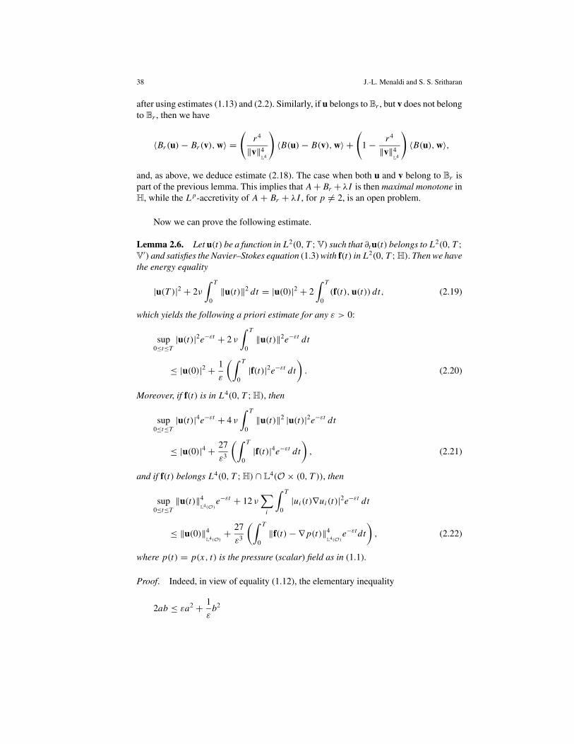
Lemma 2.6. Let u(t) be a function in L2(0, T ; V) such that ∂t u(t) belongs to L2(0, T ;V
′) and satisfies the Navier–Stokes equation (1.3) with f(t) in L2(0, T ; H). Then we havethe energy equality
|u(T )|2 + 2ν∫ T
0‖u(t)‖2 dt = |u(0)|2 + 2
∫ T
0(f(t),u(t)) dt, (2.19)
which yields the following a priori estimate for any ε > 0:
sup0≤t≤T
|u(t)|2e−εt + 2 ν∫ T
0‖u(t)‖2e−εt dt
≤ |u(0)|2 + 1
ε
(∫ T
0|f(t)|2e−εt dt
). (2.20)
Moreover, if f(t) is in L4(0, T ; H), then
sup0≤t≤T
|u(t)|4e−εt + 4 ν∫ T
0‖u(t)‖2 |u(t)|2e−εt dt
≤ |u(0)|4 + 27
ε3
(∫ T
0|f(t)|4e−εt dt
), (2.21)
and if f(t) belongs L4(0, T ; H) ∩ L4(O × (0, T )), then
sup0≤t≤T
‖u(t)‖4L4(O)
e−εt + 12 ν∑
i
∫ T
0|ui (t)∇ui (t)|2e−εt dt
≤ ‖u(0)‖4L4(O)
+ 27
ε3
(∫ T
0‖f(t)− ∇ p(t)‖4
L4(O)e−εt dt
), (2.22)
where p(t) = p(x, t) is the pressure (scalar) field as in (1.1).
Proof. Indeed, in view of equality (1.12), the elementary inequality
2ab ≤ εa2 + 1
εb2
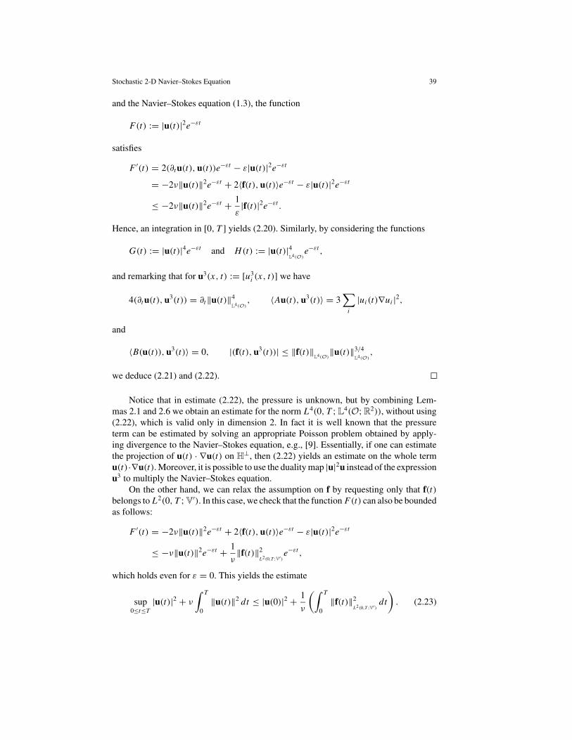
Stochastic 2-D Navier–Stokes Equation 39
and the Navier–Stokes equation (1.3), the function
F(t) := |u(t)|2e−εt
satisfies
F ′(t) = 2(∂t u(t),u(t))e−εt − ε|u(t)|2e−εt
= −2ν‖u(t)‖2e−εt + 2〈f(t),u(t)〉e−εt − ε|u(t)|2e−εt
≤ −2ν‖u(t)‖2e−εt + 1
ε|f(t)|2e−εt .
Hence, an integration in [0, T ] yields (2.20). Similarly, by considering the functions
G(t) := |u(t)|4e−εt and H(t) := |u(t)|4L4(O)
e−εt ,
and remarking that for u3(x, t) := [u3i (x, t)] we have
4(∂t u(t),u3(t)) = ∂t‖u(t)‖4L4(O)
, 〈Au(t),u3(t)〉 = 3∑
i
|ui (t)∇ui |2,
and
〈B(u(t)),u3(t)〉 = 0, |(f(t),u3(t))| ≤ ‖f(t)‖L4(O)
‖u(t)‖3/4L4(O)
,
we deduce (2.21) and (2.22).
Notice that in estimate (2.22), the pressure is unknown, but by combining Lem-mas 2.1 and 2.6 we obtain an estimate for the norm L4(0, T ; L
4(O; R2)), without using
(2.22), which is valid only in dimension 2. In fact it is well known that the pressureterm can be estimated by solving an appropriate Poisson problem obtained by apply-ing divergence to the Navier–Stokes equation, e.g., [9]. Essentially, if one can estimatethe projection of u(t) · ∇u(t) on H
⊥, then (2.22) yields an estimate on the whole termu(t)·∇u(t). Moreover, it is possible to use the duality map |u|2u instead of the expressionu3 to multiply the Navier–Stokes equation.
On the other hand, we can relax the assumption on f by requesting only that f(t)belongs to L2(0, T ; V
′). In this case, we check that the function F(t) can also be boundedas follows:
F ′(t) = −2ν‖u(t)‖2e−εt + 2〈f(t),u(t)〉e−εt − ε|u(t)|2e−εt
≤ −ν‖u(t)‖2e−εt + 1
ν‖f(t)‖2
L2(0,T ;V′)e−εt ,
which holds even for ε = 0. This yields the estimate
sup0≤t≤T
|u(t)|2 + ν
∫ T
0‖u(t)‖2 dt ≤ |u(0)|2 + 1
ν
(∫ T
0‖f(t)‖2
L2(0,T ;V′)dt
). (2.23)

40 J.-L. Menaldi and S. S. Sritharan
Similarly, if f(t) is in L4(0, T ; V′), then
sup0≤t≤T
|u(t)|4e−εt + 2 ν∫ T
0‖u(t)‖2 |u(t)|2e−εt dt
≤ |u(0)|4 + 2
ν2ε
(∫ T
0‖f(t)‖4
L2(0,T ;V′)e−εt dt
), (2.24)
for any ε > 0.By means of estimate (2.8) we check that the above estimate (2.11) and Lemmas 2.4
and 2.6 remain true in 3-D. However, estimate (2.21) is not sufficient to ensure a boundin the space L4(� × (0, T )), since we need to bound the V-norm in L3(0, T ), seeestimate (2.5).
Remark 2.7. In general, if u(t) belongs to H∩H2(O,R2), then �u(t) (∇u(t), respec-
tively) does not necessarily belong to H (V, respectively). However, the norms |� · |(|∇ ·|, respectively) and |A · | (|A1/2 · |, respectively) are equivalent (for instance, we referto [21] for details and more comments). Let u(t) satisfy the Navier–Stokes equation (1.3)with f(t) in L2(0, T ; H). If u(t) belongs to L2(0, T ; H
2(O,R2)) and ∂t u(t) belongs toL2(0, T ; H), then multiplying (1.3) by −P
H�u(t) we have
12∂t |∇u(t)|2 + ν|P
H�u(t)|2 = 〈B(u(t)),�u(t)〉 − (f(t),�u(t)), (2.25)
after recalling that here PHf(t) = f(t). Since |P
H�u| is equivalent to |�u|, there is a
constant c > 0 such that
|〈B(u),�u〉| ≤ 2|�u| |∇u|L4 |u|L4 ≤ c|�u|3/2 |∇u|1/2 |u|L4 (2.26)
and we obtain
∂t |∇u(t)|2 + ν|PH�u(t)|2 ≤ cν |u(t)|4
L4 |∇u(t)|2 + |f(t)| |�u(t)|, (2.27)
for some constant cν . Then an estimate on u(t) in the spaces L∞(0, T ; V) and L2(0, T ;H
2(O,R2)) is established.
3. Stochastic PDE
Here we look at the compact formulation (1.3) of the Navier–Stokes equation subject toa random (Gaussian) term, i.e., the forcing field f has a mean value still denoted by f anda noise denoted by G. We can write f(t) = f(t, x) and the noise process G(t) = G(t, x)as a series dGk = ∑
k gk dwk , where g = (g1, g2, . . .) and w = (w1, w2, . . .) areregarded as �2-valued functions. The stochastic noise process represented by g dw(t) =∑
k gk(t, x) dwk(t, ω) (notice that most of the time we omit the variable ω) is normaldistributed in H with a trace-class co-variance operator denoted by g∗g(t) and given by
(g∗g(t)u, v) :=
∑k
(gk(t),u) (gk(t), v),
Tr(g∗g(t)) :=∑
k
|gk(t)|2 < ∞,(3.1)

Stochastic 2-D Navier–Stokes Equation 41
i.e., the mapping (stochastic integral) induced by the noise
v �→∫ T
0(g(t) dw(t), v) :=
∑k
∫ T
0(gk(t), v) dwk(t) (3.2)
is a continuous linear functional on H with probability 1 and the noise is the formaltime-derivative of the Gaussian process G(t) = ∫ t
0 g(t) dw(t).We interpret the stochastic Navier–Stokes equation as an Ito stochastic equation in
variational form
d(u(t), v)+ 〈Au(t)+ B(u(t)), v〉 dt = (f(t), v) dt +∑
k
(gk(t), v) dwk(t), (3.3)
in (0, T ), with the initial condition
(u(0), v) = (u0, v), (3.4)
for any v in the space V. This requires the following assumption on the data:
f ∈ L2(0, T ; V), g ∈ L2(0, T ; �2(H)), u0 ∈ H, (3.5)
and we expect a solution as an adapted (and measurable) stochastic process u =u(t, x, ω) satisfying
u ∈ L2(�; C0(0, T ; H)) ∩ L2(�; L2(0, T ; V)) (3.6)
and the (linear) energy equality
d|u(t)|2 + 2ν |∇u(t)|2 dt
= Tr(g∗g(t)) dt + 2 (f(t),u(t)) dt + 2∑
k
(gk(t),u(t)) dwk(t), (3.7)
where we have used the estimate
E
{∣∣∣∣∫ T
0(g(t) dw(t), v(t))
∣∣∣∣2}
≤(∫ T
0Tr(g∗g(t)) dt
)(sup
0≤t≤TE |v(t)|2
)(3.8)
for any adapted process v with values in L∞(0, T ; H), to make the stochastic integralmeaningful. Actually, a more general martingale estimate holds, namely
E
{sup
0≤t≤T
∣∣∣∣∫ t
0(g dw(s), v(s))
∣∣∣∣p}
≤ Cp E
(∫ T
0
∑k
(gk(t), v(t))2 dt
)p/2 , (3.9)
for any 1 ≤ p < ∞ and some constant Cp depending only on p, e.g., we may takeC2 = 2 and C1 = 3.
Moreover, if we also assume that
f ∈ L4(0, T ; L4(O)), g ∈ L4(0, T ; �2(L
4(O))), u0 ∈ L4(O), (3.10)

42 J.-L. Menaldi and S. S. Sritharan
then we have the (linear) L4-energy equality
d‖u(t)‖4L4(O)
+ 12 ν∑
i
|ui (t)∇ui (t)|2 dt
=∑
k
(gk(t),u(t))2 dt + 4 (f(t)− ∇ p(t),u3(t)) dt
+ 4∑
k
(gk(t),u3(t)) dwk(t), (3.11)
where u3(x, t, ω) := [u3i (x, t, ω)] and p = p(x, t, ω) is the pressure. As mentioned
before, the pressure (scalar) field p is unknown, so that equality (3.11) is of limitedhelp.
A finite-dimensional (Galerkin) approximation of the stochastic Navier–Stokesequation (3.3) can be defined as follows. Let {e1, e2, . . .} be a complete orthonormalsystem (i.e., a basis) in the Hilbert space H belonging to the space V (and L
4). Denoteby Hn the n-dimensional subspace of H and V of all linear combinations of the first nelements {e1, e2, . . . , en}. Consider the following stochastic ODE in Hn (i.e., essentiallyin R
n):
d(un(t), v)+ 〈Aun(t)+ B(un(t)), v〉 dt
= (f(t), v) dt +∑
k
(gk(t), v) dwk(t), (3.12)
in (0, T ), with the initial condition
(u(0), v) = (u0, v), (3.13)
for any v in the space Hn . The coefficients involved are locally Lipschitz, so that we needsome a priori estimate to show the global existence of a solution un(t) as an adaptedprocess in the space C0(0, T,Hn).
Proposition 3.1 (Energy Estimate). Assume the data f, g and u0 satisfying condition(3.5). Let un(t) be an adapted process in the space C0(0, T,Hn) solution of the stochasticODE (3.12). Then we have the energy equality
d|un(t)|2 + 2ν |∇un(t)|2dt
= [2 (f(t),un(t))+ Tr(g∗g(t))] dt + 2∑
k
(gk(t),un(t)) dwk(t), (3.14)
which yields the following a priori estimate for any ε > 0:
E{|un(t)|2}e−εt + 2 ν∫ T
0E{|∇un(t)|2}e−εt dt
≤ |u(0)|2 +∫ T
0
[1
ε|f(t)|2 + Tr(g∗g(t))
]e−εt dt, (3.15)

Stochastic 2-D Navier–Stokes Equation 43
for any 0 ≤ t ≤ T . Moreover, if we suppose
f ∈ L p(0, T ; H), g ∈ L p(0, T ; �2(H)), (3.16)
then we also have
E
{sup
0≤t≤T|un(t)|pe−εt + p ν
∫ T
0|∇un(t)|2|un(t)|p−2e−εt dt
}
≤ |u(0)|p + Cε,p,T
∫ T
0[|f(t)|p + Tr(g∗g(t))p/2]e−εt dt, (3.17)
for some constant Cε,p,T depending only on ε > 0, 1 ≤ p < ∞ and T > 0.
Proof. Indeed, we notice first that (3.12) implies that
dun(t)+ [Anun(t)+ Bn(un(t))] dt = f n(t) dt +∑
k
gnk (t) dwk(t), (3.18)
where An , Bn(·), fn(t) and gnk (t) are the orthogonal projection on the finite-dimensional
subspace H′n , the dual space of Hn . Hence, by using Ito’s formula with the process un(t)
and the function u �→ |u|2, we obtain the energy equality (3.14) after noticing that(Bn(un(t)),un(t)) = (B(un(t)),un(t)) = 0.
Next, as in Lemma 2.6 we calculate the stochastic differential of the process F(t) :=|un(t)|2e−εt to get
dF(t) = e−εt d|un(t)|2 − ε|un(t)|2e−εt dt
= −2ν‖un(t)‖2e−εt dt + [2 (f(t),un(t))+ Tr(g∗g(t))]e−εt dt
+ 2∑
k
(gk(t),un(t))e−εt dwk(t),
which yields the a priori estimate (3.15).Similarly, consider G(t) := |un(t)|pe−εt and use Ito calculus based on the en-
ergy process |un(t)|2. As in Lemma 2.6, we check that its stochastic differentialsatisfies
dG(t)+ p ν‖un(t)‖2|un(t)|p−2e−εt dt + ε|un(t)|pe−εt dt
=[
p (f(t),un(t))+ p
2Tr(g∗g(t))
]|un(t)|p−2e−εt dt
+ p(p − 2)
8
∑k
(gk(t),un(t))2|un(t)|p−4e−εt dt
+ p∑
k
(gk(t),un(t))|un(t)|p−2e−εt dwk(t).
Hence, by means of the elementary inequality
ab ≤ a p
p+ aq
q,
1
p+ 1
q= 1, ab > 0,
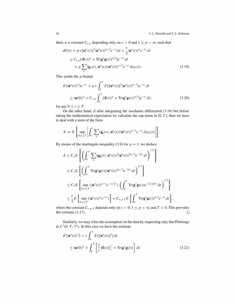
44 J.-L. Menaldi and S. S. Sritharan
there is a constant Cε,p depending only on ε > 0 and 1 ≤ p < ∞ such that
dG(t)+ p ν‖un(t)‖2|un(t)|p−2e−εt dt + ε
2|un(t)|pe−εt dt
≤ Cε,p[|f(t)|p + Tr(g∗g(t))p/2]e−εt dt
+ p∑
k
(gk(t),un(t))|un(t)|p−2e−εt dwk(t). (3.19)
This yields the p-bound
E{|un(t)|p}e−εt + p ν∫ T
0E{‖un(t)‖2|un(t)|p−2}e−εt dt
≤ |u(0)|p + Cε,p
∫ T
0[|f(t)|p + Tr(g∗g(t))p/2]e−εt dt, (3.20)
for any 0 ≤ t ≤ T .On the other hand, if after integrating the stochastic differential (3.19) but before
taking the mathematical expectation we calculate the sup norm in [0, T ], then we haveto deal with a term of the form
A := E
{sup
0≤t≤T
∣∣∣∣∣∫ t
0
∑k
(gk(s),un(s))|un(s)|p−2e−εs dwk(s)
∣∣∣∣∣}.
By means of the martingale inequality (3.9) for p = 1, we deduce
A ≤ C1 E
(∫ T
0
∑k
(gk(t),un(t))2|un(t)|2p−4e−2εt dt
)1/2
≤ C1 E
{(∫ T
0Tr(g∗g(t))|un(t)|2p−2e−2εt dt
)1/2}
≤ C1 E
{sup
0≤t≤T(|un(t)|p−1e−εt/p′
)
(∫ T
0Tr(g∗g(t))e−(2/p)εt dt
)1/2}
≤ ε
2E
{sup
0≤t≤T(|un(t)|pe−εt )
}+ Cε,p,T E
{∫ T
0Tr(g∗g(t))p/2e−εt dt
},
where the constant Cε,p,T depends only on ε > 0, 1 ≤ p < ∞ and T > 0. This providesthe estimate (3.17).
Similarly, we may relax the assumption on the data by requesting only that f belongsto L2(0, T ; V
′). In this case we have the estimate
E{|un(t)|2} + ν
∫ T
0E{‖un(t)‖2} dt
≤ |u(0)|2 +∫ T
0
[1
ν‖f(t)‖2
V′ + Tr(g∗g(t))]
dt (3.21)
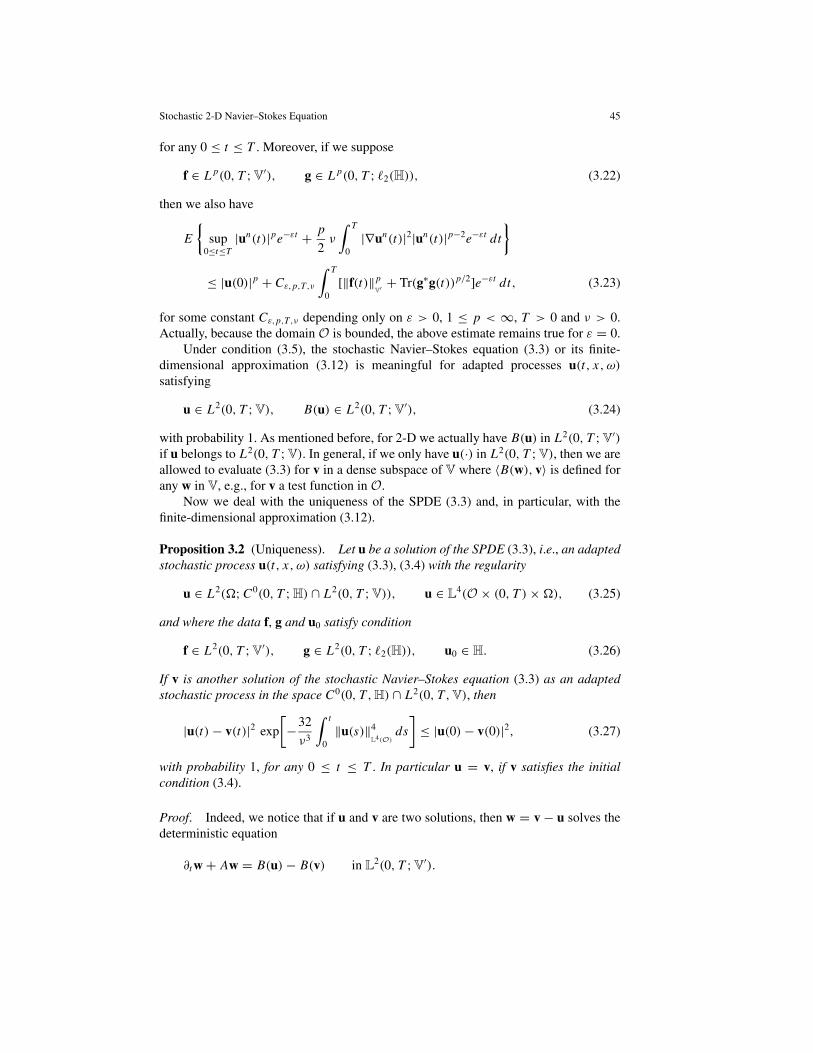
Stochastic 2-D Navier–Stokes Equation 45
for any 0 ≤ t ≤ T . Moreover, if we suppose
f ∈ L p(0, T ; V′), g ∈ L p(0, T ; �2(H)), (3.22)
then we also have
E
{sup
0≤t≤T|un(t)|pe−εt + p
2ν
∫ T
0|∇un(t)|2|un(t)|p−2e−εt dt
}
≤ |u(0)|p + Cε,p,T,ν
∫ T
0[‖f(t)‖p
V′ + Tr(g∗g(t))p/2]e−εt dt, (3.23)
for some constant Cε,p,T,ν depending only on ε > 0, 1 ≤ p < ∞, T > 0 and ν > 0.Actually, because the domain O is bounded, the above estimate remains true for ε = 0.
Under condition (3.5), the stochastic Navier–Stokes equation (3.3) or its finite-dimensional approximation (3.12) is meaningful for adapted processes u(t, x, ω)satisfying
u ∈ L2(0, T ; V), B(u) ∈ L2(0, T ; V′), (3.24)
with probability 1. As mentioned before, for 2-D we actually have B(u) in L2(0, T ; V′)
if u belongs to L2(0, T ; V). In general, if we only have u(·) in L2(0, T ; V), then we areallowed to evaluate (3.3) for v in a dense subspace of V where 〈B(w), v〉 is defined forany w in V, e.g., for v a test function in O.
Now we deal with the uniqueness of the SPDE (3.3) and, in particular, with thefinite-dimensional approximation (3.12).
Proposition 3.2 (Uniqueness). Let u be a solution of the SPDE (3.3), i.e., an adaptedstochastic process u(t, x, ω) satisfying (3.3), (3.4) with the regularity
u ∈ L2(�; C0(0, T ; H) ∩ L2(0, T ; V)), u ∈ L4(O × (0, T )×�), (3.25)
and where the data f, g and u0 satisfy condition
f ∈ L2(0, T ; V′), g ∈ L2(0, T ; �2(H)), u0 ∈ H. (3.26)
If v is another solution of the stochastic Navier–Stokes equation (3.3) as an adaptedstochastic process in the space C0(0, T,H) ∩ L2(0, T,V), then
|u(t)− v(t)|2 exp
[−32
ν3
∫ t
0‖u(s)‖4
L4(O)ds
]≤ |u(0)− v(0)|2, (3.27)
with probability 1, for any 0 ≤ t ≤ T . In particular u = v, if v satisfies the initialcondition (3.4).
Proof. Indeed, we notice that if u and v are two solutions, then w = v − u solves thedeterministic equation
∂t w + Aw = B(u)− B(v) in L2(0, T ; V
′).
46 J.-L. Menaldi and S. S. Sritharan
Setting
r(t) := 32
ν3
∫ t
0‖u(s)‖4
L4(O)ds
and using Lemma 2.4 we have
d(e−r(t)|w(t)|2)+ νe−r(t)‖w(t)‖2dt
= −r(t)e−r(t)|w(t)|2 dt − νe−r(t)‖w(t)‖2 dt
− 2e−r(t)〈B(v(t))− B(u(t)),w(t)〉 dt ≤ 0.
Hence, integrating in t , we deduce (3.27), with probability 1.
Notice that a solution u of the stochastic Navier–Stokes equation (3.3) in thespace L2(�; L∞(0, T ; H) ∩ L2(0, T ; V)) actually belongs to a better space, namelyL2(�; C0(0, T ; H)∩L
4(O× (0, T ))), with O ⊂ R2. Thus in 2-D, the uniqueness holds
in the space L2(�; L2(0, T ; V)). Clearly, this also applies to the finite-dimensional ap-proximation (3.12) in the space L2(�; L2(0, T ; Hn)), but it is not needed there sincethe coefficients are locally Lipschitz in Hn . We also note that an argument similar to theabove was used in [19] for the uniqueness of solutions with multiplicative noise.
Let r(t, ω) be the integral on [0, t] of an adapted, non-negative and integrablestochastic process r(t, ω). It is clear that for any (adapted process) solution u of thestochastic Navier–Stokes equation (3.3) such that
u ∈ L2(�; L∞(0, T ; H) ∩ L2(0, T ; V)), (3.28)
the new process u := ue−r satisfies
d(u(t), v)+ 〈Au(t)+ e−r(t)B(u(t))+ r(t)u(t), v〉 dt
= (e−r(t)f(t), v) dt +∑
k
(e−r(t)gk(t), v) dwk(t), (3.29)
for any function v in V ∩ L∞(O). Conversely, if u(t) is any (adapted process) solution
of (3.29), such that u := uer satisfies (3.28), then u is indeed a solution of the stochasticNavier–Stokes equation (3.3).
Regarding the energy equality, we remark that for a given adapted process u(x, t, ω)in L2(�; L∞(0, T ; H) ∩ L2(0, T ; V)) satisfying
d(u(t), v) = 〈h(t), v〉 dt + (g(t), v) dw(t), (3.30)
for any function v in V and some h in L2(0, T ; V′) and g in L2(0, T ; �2(H)), we can
find a version of u (still denoted by u) in the space L2(�; C0(0, T ; H)), and the energyequality
d|u(t)|2 = [2〈h(t),u(t)〉 + Tr(g∗g(t)] dt + 2(g(t),u(t)) dw(t) (3.31)
holds, for instance see [11]. In our context, any solution of the stochastic Navier–Stokes equation (3.3) satisfying (3.28) has a continuous version, i.e., in the space
Stochastic 2-D Navier–Stokes Equation 47
L2(�,C0([0, T ],H)) such that the energy equality
d|u(t)|2 + 2ν |∇u(t)|2 dt
= Tr(g∗g(t) dt + 2 (f(t),u(t)) dt + 2∑
k
(gk(t),u(t)) dwk(t), (3.32)
i.e., (3.7), holds.
Proposition 3.3 (2-D Existence). Let f, g and u0 be such that
f ∈ L p(0, T ; V′), g ∈ L p(0, T ; �2(H)), u0 ∈ H, (3.33)
for some p ≥ 4. Then there exists an adapted process u(t, x, ω) with the regularity
u ∈ L p(�; C0(0, T ; H)) ∩ L2(�; L2(0, T ; V)) ∩ L4(O×(0, T )×�) (3.34)
and satisfying (3.3), (3.4).
Proof. Indeed, denoting by F(u) the operator νAu + B(u)− f we have
dun(t)+ F(un(t)) dt = g dw(t), in H′n,
and based on the a priori estimates (3.23) we can extract a subsequence such that
un −→ u weakly star in L p(�; L∞(0, T ; H)) ∩ L2(�; L2(0, T ; V)),
F(un) −→ F0 weakly in L2(�; L2(0, T ; V′)),
where u has the Ito differential
du(t)+ F0(t) dt = g(t) dw(t),
in L2(�; L2(0, T ; V′)), and the energy equality holds, i.e.,
d|u(t)|2 + 2〈F0(t),u(t)〉 dt = Tr(g∗g(t)) dt + 2(g(t),u(t)) dw(t).
Notice that we also have |un(0) − u(0)| goes to 0 in L2(�) and that un converges to uweakly star in the Banach space L p(�; C0(0, T ; H)) so that t �→ u(t) is a continuousfunction from [0, T ] into H with probability 1.
Now, for any adapted process v(t, x, ω) in L∞((0, T ) × �; Hm), with m ≤ n wedefine
r(t, ω) := 32
ν3
∫ t
0‖v(s, ·, ω)‖4
L4(O)ds
as an adapted, continuous (and bounded in ω) real-valued process in [0, T ]. From theenergy equality
E{de−r(t)|un(t)|2 + e−r(t)〈2F(un(t))+ r(t)un(t),un(t)〉 dt}= E{e−r(t) Tr(gn
∗gn(t) dt},
48 J.-L. Menaldi and S. S. Sritharan
the fact that the initial condition un(0) converges in L2, and the lower-semi-continuity
of the L2-norm, we deduce
lim infn
E
{−∫ T
0e−r(t)〈2F(un(t))+ r(t)un(t),un(t)〉 dt
}
= lim infn
E
{e−r(T )|un(T )|2 − |un(0)|2 −
∫ T
0e−r(t) Tr(gn
∗gn(t)) dt
}
≥ E
{e−r(T )|u(T )|2 − |u(0)|2 −
∫ T
0e−r(t) Tr(g∗g(t)) dt
}
= E
{−∫ T
0e−r(t)〈2F0(t)+ r(t)u(t),u(t)〉 dt
}.
Next, in view of Lemma 2.4 (monotonicity on L4-balls) we have
E
{∫ T
0e−r(t)〈2F(v(t))+ r(t)v(t), v(t)− un(t)〉 dt
}
≥ E
{∫ T
0e−r(t)〈2F(un(t))+ r(t)un(t), v(t)− un(t)〉 dt
},
and taking limit in n we obtain
E
{∫ T
0e−r(t)〈2F(v(t))+ r(t)v(t), v(t)− u(t)〉 dt
}
≥ E
{∫ T
0e−r(t)〈2F0(t)+ r(t)u(t), v(t)− u(t)〉 dt
}. (3.35)
Since this last inequality holds for every v in L∞((0, T )×�; Hm) and any m, a density ar-gument show that (3.35) remains true for any adapted process v in L6(�; L∞(0, T ; H))∩L2(�; L2(0, T ; V)) such that
E
{∫ T
0‖v(t, ·, ω)‖4
L4(O)|v(t, ·, ω)− u(t, ·, ω)|2 dt
}< ∞.
In 2-D we can control the L4(O×(0, T ))-norm with the norms in the spaces L∞(0, T ; H)
and L2(0, T ; V), see (2.2) of Lemma 2.1, so that the process u satisfies the above condi-tion. In 3-D we may compare (2.2) with estimate (2.5), where only the L3(0, T ; L
4(O))can be bounded.
Hence, first we take v := u + λw, with λ > 0 and w an adapted process inL4(�; L∞(0, T ; H)) ∩ L2(�; L2(0, T ; V)). Next we divide by λ and finally we let λvanish in (3.35) to deduce
E
{∫ T
0e−r(t)〈F(u(t))− F0(t),w(t)〉 dt
}≥ 0,
and because w is arbitrary, we conclude that F0(t) = F(u(t)). This proves that u is asolution of the stochastic Navier–Stokes equation (3.3).
Stochastic 2-D Navier–Stokes Equation 49
The technique to identify the limiting drift F0(t) in (3.35) is a variant of the classicargument used for the monotone operator, see [16] and [18]. The semigroup technique,as in Chapter 15 of [8], provides a pathwise (or mild) solution by means of a stochasticconvolution and the change of unknown function u := u + WA, where
WA(t) :=∑
k
∫ t
0exp[(t − s)A]gk(s) dwk(s). (3.36)
The (deterministic, with random data) mild equation is as follows:
∂t u + Au + B(u + WA) = f in L2(0, T ; H) ∩ L
4(O × (0, T )), (3.37)
with an initial condition in H. The technique of Proposition 3.3 can be used with thepathwise equation (3.37) to give another proof of the existence of a pathwise (mild)solution.
When the domain O in R2 is unbounded, we need to use the norm
‖v‖V
:=(∫
O|v|2 + |∇v|2 dx
)1/2
, (3.38)
instead of (1.6) for the space V, so that it will be continuously embedded in H. In thiscase, the a priori estimates (3.17) in Proposition 3.1 and (3.23) remain the same, namely
E
{sup
0≤t≤T|un(t)|pe−εt + p
2ν
∫ T
0|∇un(t)|2|un(t)|p−2e−εt dt
}
≤ |u(0)|p + Cε,p,T,ν
∫ T
0[‖f(t)‖p
V′ + Tr(g∗g(t))p/2]e−εt dt, (3.39)
for some constant Cε,p,T,ν depending only on ε > 0, 1 ≤ p < ∞, T > 0 and ν > 0.Here we need ε > 0 to compensate the seminorm |∇ · | with the norm (3.38) in thespace V. Since we can still control the L
4(O)-norm in terms of the L2(O)-norms, see
estimate (2.2) in Lemma 2.1, the existence and uniqueness results hold for unbounded 2-D domains. On the contrary, in 3-D, estimates in the spaces L2(0, T,V) and L∞(0, T,H)are not enough to ensure a bound in L
4(�× (0, T )) and the above results are not longervalid.
We may use as initial time τ a stopping time (random variable) with respect tothe natural filtration (Ft , t ≥ 0) (right-continuous and completed) associated with theWiener process, and initial value u0 = uτ (x, ω) which is an Fτ -measurable randomvariable. Similarly, we may allow random forcing terms f(x, t, ω) and g(x, t, ω) or evenhave a smooth dependency on the solution u. For the random initial conditions we haveto write the stochastic Navier–Stokes equation (3.3), (3.4) in its integral (variational)form, namely
(u(θ), v)+∫ θ
τ
〈Au(t)+ B(u(t)), v〉 dt
= (uτ , v)+∫ θ
τ
(f(t), v) dt +∑
k
∫ θ
τ
(gk(t), v) dwk(t), (3.40)
50 J.-L. Menaldi and S. S. Sritharan
for any stopping time τ ≤ θ ≤ T and any v in the space V. Actually, by a density argumentwe may allow any adapted process v(t) in L2(�; L2(τ, T ; V)) ∩ L
4(O × (τ, T )×�).We state the following result valid for smooth domains O in R
2 not necessarily bounded.
Proposition 3.4 (2-D). Let τ and uτ be a stopping time with respect to (Ft , t ≥ 0)and an Fτ -measurable random variable such that
0 ≤ τ ≤ T, uτ ∈ L4(�; H). (3.41)
Suppose f(x, t, ω) and g(x, t, ω) are adapted processes such that
f ∈ L4((τ, T )×�; V′), g ∈ L4((τ, T )×�; �2(H)). (3.42)
Then there exists an adapted process u(t, x, ω) with the regularity
u ∈ L4(�; C0(τ, T ; H)) ∩ L2((τ, T )×�; V)) (3.43)
and satisfying (3.40) and the following a priori bound holds for p ≥ 2:
E
{supτ≤t≤T
|u(t)|pe−εt + p
2ν
∫ T
τ
|∇u(t)|2|u(t)|p−2e−εt dt
}
≤ E
{|u(τ )|p + Cε,T,ν
∫ T
τ
[‖f(t)‖pV′ + Tr(g∗g(t))p/2]e−εt dt
}, (3.44)
for some constant Cε,T,ν depending only on ε > 0, T > 0 and ν > 0. Moreover, ifu(t, x, ω) is the solution with another initial data, we have
|u(θ)− u(θ)|2 exp
[−32
ν3
∫ θ
τ
‖u(t)‖4L4(O)
dt
]≤ |uτ − u(τ )|2, (3.45)
with probability 1, for any τ ≤ θ ≤ T .
Proof. This is a consequence of previous propositions and the above comments. Noticethat we set u(t) := uτ for any 0 ≤ t ≤ τ .
This proposition is stochastic analogous to the classic results in [14].Notice that we have
‖u(t)‖4L4(O)
≤ 2|u(t)|2 |∇u(t)|2, (3.46)
so that a priori estimate (3.44) contains the regularity conditions
u ∈ L4(O × (0, T )×�). (3.47)
Moreover, the (linear) energy equality (3.7) and estimate
E{|u(θ)|2}e−εθ + νE
{∫ θ
τ
‖u(t)‖2e−εt dt
}
≤ E{|uτ |2e−ετ } + E
{∫ θ
τ
[1
min{ν, ε}‖f(t)‖2V′ + Tr(g∗g(t))
]e−εt dt
}(3.48)

Stochastic 2-D Navier–Stokes Equation 51
hold. Furthermore, if the domain O is bounded or forcing term f(t) is such that for someconstant C = Cf we have
E
{∫ T
0sup
|∇v|≤1|〈f(t), v〉|4 dt
}≤ Cf, (3.49)
then we may replace the min{ν, ε} with ν in estimate (3.48) and set ε = 0.For additive noise, a key point used by Bensoussan and Temam [4] and Flandoli
and Gatarek [10] is the comparison of the stochastic Navier–Stokes solution (3.3) withthe solution of the linear equation
dv(t)+ Av(t) dt =∑
k
gk(t) dwk(t),
which yields the deterministic Navier–Stokes-type equation
w + Aw + B(w + v) = f,
for the unknown w = u − v, and, therefore, the existence of a strong solution can bededuced. However, our technique can also be used with multiplicative noise. Indeed,if the noise takes the form g(t, u) dw(t) = ∑
k gk(t, x, u) dwk(t), where g(t, u) is acontinuous operator from V into L2(0, T ; �2(H)), we can modify the calculations in theabove propositions under the assumption: there is a λ > 0 such that for some 0 < ν ′ < ν
we have∑k
|gk(t, u)− gk(t, v)|2H + λ|u − v|2H
≤ ν ′|∇u − ∇v|2H, ∀u, v ∈ V.
Thus the existence and uniqueness of a strong solution holds even for multiplicativenoise.
Remark 3.5 (V -Regularity). It is clear that if the adapted processes f and g satisfy
f ∈ L2((0, T )×�; H), g ∈ L2((0, T )×�; �2(V)), (3.50)
then the arguments of Remark 2.7 show that the solution of the 2-D stochastic Navier–Stokes equation (3.3) satisfies
u ∈ C0(0, T ; V) ∩ L2(0, T ; H2(O,R2)), (3.51)
with probability 1, provided the initial data uτ is in V. More details are needed to obtainan estimate similar to (3.44). Notice that the above assumption (3.50) on the Hilbert–Schmidt operator g(t) means that
∑k ‖gk(t)‖2 is integrable in (0, T )×�. Hence, if O
is bounded, we can follow the arguments in Chapter 15 of [8] to deduce the existence ofan invariant measure.
We consider the space C0p(H) of real continuous functions h on H with a p-growth,
0 ≤ p < ∞, i.e.,
|h(v)| ≤ Ch(1 + |v|p), ∀ v ∈ H. (3.52)

52 J.-L. Menaldi and S. S. Sritharan
When p = 0, we have all continuous and bounded real functions on the Hilbert spaceH. We define the (linear) Navier–Stokes semigroup (�(t, s), t ≥ s ≥ 0) as follows:
�(t, s): C0p(H) −→ C0
p(H), �(t, s)h(v) := E{h(u(t, s; v))}, (3.53)
where u(t, s; v) denotes the solution u(x, t, ω) of the stochastic Navier–Stokes equa-tion (3.3) with initial (deterministic) value u(x, s, ω) = v(x). We have
Proposition 3.6 (Markov-Feller). Suppose we are given two adapted processes f(x, t,ω) and g(x, t, ω) satisfying condition (3.42) of the previous proposition. Then (�(t, s),t ≥ s ≥ 0) is a Markov–Feller semigroup on the space C0
p(H), for any 0 ≤ p < 6.
Proof. The uniqueness of solutions yields the semigroup property. Next, by definitionwe have that h(v) ≥ 0 for all v implies �(t, s)h(v) ≥ 0 for all v. Thus we need onlycheck the Feller property and the pointwise convergence at t = s, i.e., for any functionh in C0
p(H){vn → v in H implies �(t, s)h(vn) → �(t, s)h(v),
tn → s in R+ implies �(tn, s)h(v) → h(v),
(3.54)
for any v in H. Indeed, to show (3.54) we notice that from estimate (3.45) and thecontinuity of h we deduce that h(vn) converges to h(v) in R with probability 1, andbecause the solution u(t, s; v) belongs to L2(�; C0(s, T ; H))we have that h(u(tn, s; v))converges to h(v) in R with probability 1. Hence, the a priori estimate (3.44) lets us takethe limits inside the integral for any p < 4.
It is clear that if we need to work in a space C0p(H) for some p ≥ 4 we need to
require conditions (3.41) and (3.42) for some q > p instead of just 4.A realization in the canonical space C0(0, T ; H) of the Markov–Feller process
associated with the above semigroup is given by the random field u(t, s; v), t > s > 0,v in H, i.e., the solution of stochastic PDE (3.40) with initial value τ = s and vτ = v.
References
1. Adams RA (1975) Sobolev Spaces, Academic Press, New York2. Barbu V, Sritharan SS (2001) Flow invariance preserving feedback controllers for the Navier–Stokes
equation, J Math Anal Appl 255:281–3073. Bensoussan A (1995) Stochastic Navier–Stokes equations, Acta Appl Math 38:267–3044. Bensoussan A, Temam R (1973) Equations stochastique du type Navier–Stokes, J Funct Anal 13:195–2225. Capinski M, Cutland NJ (1995) Nonstandard Methods for Stochastic Fluid Mechanics, World Scientific,
Singapore6. Chandrasekhar S (1989) Stochastic, Statistical and Hydromagnetic Problems in Physics and Astronomy,
Selected Papers, Vol 3, University of Chicago Press, Chicago7. Constantin P, Foias C (1988) Navier–Stokes Equations, University of Chicago Press, Chicago8. Da Prato G, Zabczyk J (1996) Ergodicity for Infinite Dimensional Systems, Cambridge University Press,
Cambridge9. Da Veiga HB (1987) Existence and asymptotic behavior for strong solutions of Navier–Stokes equations
in the whole space, Indiana Univ Math J 36:149–156
Stochastic 2-D Navier–Stokes Equation 53
10. Flandoli F, Gatarek D (1995) Martingale and stationary solutions for the stochastic Navier–Stokes equa-tion, Probab Theory Rel Fields 102:367–391
11. Gyongy I, Krylov NV (1982) On stochastic equations with respect to semimartingales: Ito formula inBanach spaces, Stochastics 6:153–173
12. Ladyzhenskaya OA (1969) The Mathematical Theory of Viscous Incompressible Flow, Gordon andBreach, New York
13. Lions JL (1969) Quelque methodes de resolution des problemes aux limites non lineaires, Dunod, Paris14. Lions JL, Prodi G (1959) Une theoreme d’existence et unicite dans les equations de Navier–Stokes en
dimension 2, CR Acad Sci Paris 248:3519–352115. Menaldi JL, Sritharan SS (2002) Impulse control of stochastic Navier–Stokes equations, Nonlinear Anal
Ser A, to appear16. Minty GJ (1962) Monotone (nonlinear) operators in Hilbert spaces, Duke Math J 29:341–34617. Novikov EA (1965) Functionals and random force method in turbulence theory, Soviet Phys JETP
20:1290–129418. Pardoux E (1979) Stochastic partial differential equations and filtering of diffusion processes, Stochastics
6:127–16719. Schmalfuss B (1997) Qualitative properties for the stochastic Navier–Stokes equation, Nonlinear Anal
28:1545–156320. Sritharan SS (2000) Deterministic and stochastic control of Navier–Stokes equation with linear, monotone
and hyperviscosities, Appl Math Optim 41:255–30821. Temam R (1995) Navier–Stokes Equations and Nonlinear Functional Analysis (second edition), CBMS–
NSF 66, SIAM, Philadelphia, PA22. Vishik MJ, Fursikov AV (1988) Mathematical Problems in Statistical Hydromechanics, Kluwer,
Dordrecht23. W. von Wahl (1985) The Equations of Navier–Stokes and Abstract Parabolic Equations, Vieweg,
Braunschweig
Accepted 5 May 2002. Online publication 9 September 2002.