stochastic ac optimal power flow (opf): a data-driven approach

Stochastic AC Optimal Power Flow (OPF):A Data-Driven Approach

Ilyès Mezghani, Sidhant Misra, Deepjyoti Deka

April 23, 2020

Context and personal background

• PhD student in OR and Energy at CORE/LIDAM, UCLouvain since2016 (https://uclouvain.be/fr/node/4474).

• Under the supervision of Anthony Papavasiliou(https://perso.uclouvain.be/anthony.papavasiliou).

• Part of the UCLouvain Engie Chair(http://uclengiechair.be/).

• Work done during summer 2019 at LANL, Theory Division.Group: Advanced Network Science Initiative(https://lanl-ansi.github.io/).

• Paper to appear in PSCC2020:https://arxiv.org/abs/1910.09144.

1/31

https://uclouvain.be/fr/node/4474

https://perso.uclouvain.be/anthony.papavasiliou

http://uclengiechair.be/

https://lanl-ansi.github.io/

https://arxiv.org/abs/1910.09144

Motivation

The increase in renewable generation and load flexibility comes withnew challenges.

Source: https://www.genscape.com/blog

→ Need for more reliable decisions. 2/31

https://www.genscape.com/blog/year-review-behind-meter-solar-unmasking-secret-solar-california

Research question

Lot of historical data collected by power grid operators for the samestatic power network.

How can historical data and network information be usedefficiently to ensure reliable decision making on the grid?

3/31

Agenda

1. Introduction

2. Problem Formulation

3. A Data-Driven Scenario-Based Approach

4. Numerical Experiment

5. Conclusion & Future Work

4/31

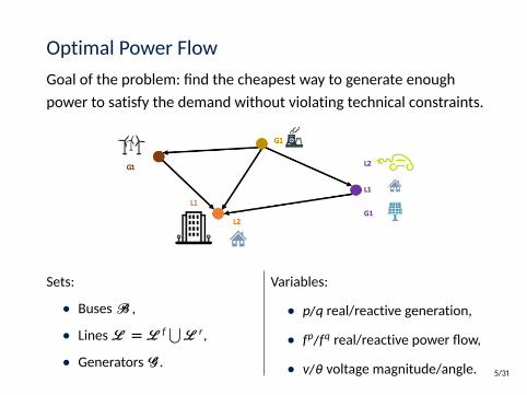
Optimal Power FlowGoal of the problem: find the cheapest way to generate enoughpower to satisfy the demand without violating technical constraints.

Sets:

• BusesB ,

• LinesL = L f⋃L r,

• Generators G .

Variables:

• p/q real/reactive generation,

• fp/fq real/reactive power flow,

• v/θ voltage magnitude/angle. 5/31

OPF and Power Flow (PF) Recourse

Deterministic OPF

min∑g∈G

c(pg) (1)

s.t.∑(i,j)∈L

fpij =∑g∈Gi

pg − Pi − Gsi v2i ∀i ∈ B (2)

∑(i,j)∈L

fqij =∑g∈Gi

qg − Qi + Bsi v2i ∀i ∈ B (3)

fpij = Giv2i − Gijvivj cos(θi − θj)

− Bijvivj sin(θi − θj) ∀(i, j) ∈ L (4)

fqij = −Biv2i + Bijvivj cos(θi − θj)

− Gijvivj sin(θi − θj) ∀(i, j) ∈ L (5)

(fpij )2 + (fqij )

2 ≤ S2ij ∀(i, j) ∈ L (6)

θij ≤ θi − θj ≤ θij ∀(i, j) ∈ L f (7)

p ≤ p ≤ p, q ≤ q ≤ q, v ≤ v ≤ v (8)

→ Non-linear, non convexoptimization problem.

PF Recourse

1. Fix (p, v) for PV buses .

2. Find (p, q, fp, fq, v, θ) bysolving (2)-(5).

→ System of non-linearequalities (easy to solve).

6/31

OPF and Power Flow (PF) Recourse

Ideally: find (p0, v0) and an ’adjustment policy’ able to react incase of perturbations.

Is this feature possible to ensure? If so, how?

We suggest:

• a formulation of Stochastic AC OPF (SACOPF).

• attacking the problem with a practical iterative approach.

7/31

Stochastic AC OPF

We’ll only assume load disturbances.Ω denotes the uncertainty set. For ω ∈ Ω, the feasible set for OPF is:

OPF(ω) =(p, q, fp, fq, v, θ) satisfying∑(i,j)∈L

fpij =∑g∈Gi

pg − (Pi + μω,pi ) − Gsi v

2i ∀i ∈ B ,∑

(i,j)∈L

fqij =∑g∈Gi

qg − (Qi + μω,qi ) + Bsi v2i ∀i ∈ B ,

and (4)− (8)

8/31

Stochastic AC OPF

Since (p, v) need to be used for recourse, we suggest the followingformulation:

(p0(Ω), v0(Ω)) = argmin∑g∈G

cg(p0g) (9)

s.t. (pω, qω, fp,ω, fq,ω, vω, θω) ∈ OPF(ω) ∀ω ∈ Ω (10)

pω = p0 +

(∑i∈B

μp,ωi

)α ∀ω ∈ Ω (11)

vω = v0 ∀ω ∈ Ω (12)

(11) and (12) define the adjustment policy.Note that α is a parameter, αg ≈ 1

|G | ∀g ∈ G .9/31

How to tackle SACOPF?

One main issue concerning Ω:

• finite but huge if based on historical data.

• inifite if based on a probability distribution.

The idea is to intelligently reduce Ω to ΩN = ω1, . . . , ωN, with Nsmall enough, and compute (p0(ΩN), v0(ΩN)) in a way thatensures feasibility for all (or most of) ω ∈ Ω.

10/31

Agenda

1. Introduction





11/31

General Idea

InitializationChoose Ω0 and

compute p0(Ω0), v0(Ω0)

SamplingTest the robustness of p0(ΩN), v0(ΩN)on a large number of samples S of Ω.

Scenario SelectionChoose n scenarios to add to ΩN.ΩN = ΩN ∪ ω1, . . . , ωn

Stochastic SolutionSolve SACOPF with ΩN to get

new p0(ΩN), v0(ΩN). 12/31

Toy ExampleOne simple way to apply the approach:

• Ω0 = ω0 where ω0 = (μp = 0, μq = 0).

• Add n random scenarios to Ω0.

Test case 73_ieee: 73 bus-system, 51 loads. We assumemax/min+/- 3% uniform perturbation of each load.

n Infeasibility PF Recourse0 1,000/1,0009 595/1,00019 250/1,00029 323/1,00039 80/1,00049 122/1,000

13/31

Practical ApproachInitialization

Choose Ω0 andcompute p0(Ω0), v0(Ω0)




new p0(ΩN), v0(ΩN).

Data-Driven SelectionMaxViol, NbConstr, Hybrid

Enhancement

14/31

Data-Driven Selection

15/31



We should use sampling information to choose the scenarios to add to ΩN.

ω0

ω1ω2

ω3 ω4


How to select ’bad’ scenarios?Example: we want to add 3 of these samples to ΩN.

• Sample s1. Constraints violated: [QgUp10,FlowLim3,VDown12].Max violation: 7.5% .

• Sample s2: Constraints violated: [QgUp10,VDown12].Max violation: 5.0% .

• Sample s3. Constraint violated: [QgUp10].Max violation: 15.0% .


• Sample s5. Constraint violated: [QgDown11].Max violation: 9.0% .

16/31


How to select ’bad’ scenarios? Max Viol.Example: we want to add 3 of these samples to ΩN.

• Sample s1. Constraints violated: [QgUp10,FlowLim3,VDown12]. 3Max violation: 7.5% .

• Sample s2: Constraints violated: [QgUp10,VDown12].Max violation: 5.0% .

• Sample s3. Constraint violated: [QgUp10]. 1Max violation: 15.0% .


• Sample s5. Constraint violated: [QgDown11]. 2Max violation: 9.0% .

16/31


How to select ’bad’ scenarios? Number of constraints.Example: we want to add 3 of these samples to ΩN.

• Sample s1. Constraints violated: [QgUp10,FlowLim3,VDown12]. 1Max violation: 7.5% .

• Sample s2: Constraints violated: [QgUp10,VDown12]. 2Max violation: 5.0% .

• Sample s3. Constraint violated: [QgUp10]. 3Max violation: 15.0% .


• Sample s5. Constraint violated: [QgDown11].Max violation: 9.0% .

16/31


How to select ’bad’ scenarios? Hybrid: weights = MVsmaxs′∈S

MVs′+ NbCs

maxs′∈S

NbCs′

Example: we want to add 3 of these samples to ΩN.

• Sample s1. Constraints violated: [QgUp10,FlowLim3,VDown12]. 1Max violation: 7.5% weights1 = 1.5.

• Sample s2: Constraints violated: [QgUp10,VDown12]. 3Max violation: 5.0% weights2 = 1.

• Sample s3. Constraint violated: [QgUp10]. 2Max violation: 15.0% weights3 = 1.33.

• Sample s4. Constraints violated: [QgUp10,FlowLim3,VDown12].Max violation: 2.2% weights4 = 1.15.

• Sample s5. Constraint violated: [QgDown11].Max violation: 9.0% weights5 = 0.93.

16/31

Toy Example

73_ieee: max/min +/- 3% uniform perturbation of each load.

• Ω0 = ω0 where ω0 = (μp = 0, μq = 0).

• Add n = 5 scenarios from the 1,000 samples to ΩN usingMaxViol, NbConstr or Hybrid selection .

n Infeasibility PF Recourse0 1,000/1,0009 595/1,00019 250/1,00029 323/1,00039 80/1,00049 122/1,000

17/31

Toy Example


• Ω0 = ω0 where ω0 = (μp = 0, μq = 0).

• Add n = 5 scenarios from the 1,000 samples to ΩN usingMaxViol, NbConstr or Hybrid selection .

Scen. Selec. # It |ΩN| PF RecourseMaxViol 5 20 1/1,000NbConstr 7 28 0/1,000Hybrid 8 29 0/1,000

Still, ΩN might be too large at the end of the iterations, especiallyfor this small test case.

17/31








Enhancement

18/31

Enhancement

After selecting ’bad’ scenarios, would it be possible to make themcapture ’more scenarios’?

ω

19/31

Enhancement

After selecting ’bad’ scenarios, would it be possible to make themcapture ’more scenarios’?

ω

Enhance(ω)

19/31

Enhance operation

Let ω be a scenario to be added to ΩN.Sc: set of sampled scenarios violating constraint c ∈ C .Cω: set of constraints violated by ω.ysc: violation of constraints c by sampled scenario s.

→ ∀c ∈ Cω, dc = argmind

∑s∈Sc

(ysc − (d0 +

∑i∈B diμsi )

)2+ λ|d|1

→ Deduce dω by gathering non zero directions of dc, c ∈ Cω.

→ ∀i ∈ B , depending on sign(dωi ),

μωi = Enhance(μωi ) = μi, μi or μω

i

. 20/31

Toy Example


• Ω0 = ω0 where ω0 = (μp = 0, μq = 0).

• n = 5, |S | = 1,000 using MaxViol, NbConstr or Hybridselection and applying Enhance.


21/31

Agenda

1. Introduction





22/31

Numerical experiment

The method works on small test cases. For these 3 test cases, weapply +/- 3 % at each load.

Test case # Loads Scen. Selec. # It |ΩN| PF Recourse24_ieee 17 MaxViol 3 7 0/1,00073_ieee 51 MaxViol 1 6 0/1,000118_ieee 99 MaxViol 3 14 0/1,000

23/31

Numerical experimentOne large test case: 1354_pegase. +/- 2% for loads located at leafbuses: 211 uncertain loads.

24/31

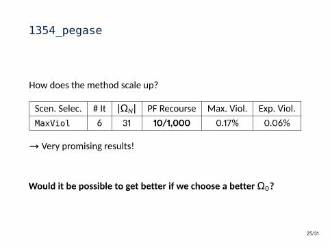
1354_pegase

How does the method scale up?

Scen. Selec. # It |ΩN| PF Recourse Max. Viol. Exp. Viol.MaxViol 6 31 10/1,000 0.17% 0.06%

→ Very promising results!

Would it be possible to get better if we choose a better Ω0?

25/31








Enhancement

Identification ofCritical Scenarios

26/31

Identification of Critical Scenarios

At the moment, we only initialize Ω0 := ω0.Could we find a better way to initialize the algorithm?

• If historical data is available, an operator would probably havean idea of what critical scenarios could be.

27/31

Identification of Critical Scenarios

At the moment, we only initialize Ω0 := ω0.Could we find a better way to initialize the algorithm?• Otherwise, we suggest to detect critical scenarios in the

following way:1. Take the deterministic solution and consider 𝜇 as a variable.2. Change the objective:Maximize violation of a certain

constraint.3. For each constraint violated→ a critical scenario.4. If necessary, cluster the critical scenarios to reduce the size of

potential Ω0.

27/31

1354_pegase

Scen. Selec. # It |ΩN| PF RecourseMaxViol 6 31 10/1,000

Applying this to 1354_pegase, we obtained 392 critical scenariosand reduced it to 11 scenarios using K-means clustering in order toget Ω0.

Scen. Selec. # It |ΩN| PF RecourseHybrid 3 25 0/1,000

28/31








Enhancement

Identification ofCritical Scenarios

29/31

Conclusion & Future Work

• The formulation of the problem and the practical approachconfirm that reliable decisions can be taken for solving AC-OPF.

• Numerical experiments seem promising:– 1354_pegase: |ΩN| = 25 for 211 perturbed loads on a 1354

bus-system.

• Future work:– Parallelization: Initialization and Sampling.– Initial clustering could be improved.– More realistic uncertainty modeling.– Extend the approach to larger and more realistic test cases.

30/31

Thank you for your attention!

Stochastic AC Optimal Power Flow:A Data-Driven Approach

https://arxiv.org/abs/1910.09144To appear in PSCC2020

Ilyès Mezghanihttps://sites.google.com/view/ilyesmezghani/home

31/31

https://arxiv.org/abs/1910.09144

https://sites.google.com/view/ilyesmezghani/home

stochastic ac optimal power flow (opf): a data-driven approach

Documents