stochastic analysis, modeling, and simulation (sams...
TRANSCRIPT
Stochastic Analysis, Modeling, and Simulation (SAMS)
Version 2007
USER's MANUAL
O. G. B. Sveinsson, J. D. Salas, W. L. Lane, and D. K. Frevert
December, 2007
Computing Hydrology Laboratory Department of Civil and Environmental Engineering
Colorado State University Fort Collins, Colorado
TECHNICAL REPORT No.11
i
Stochastic Analysis, Modeling, and
Simulation (SAMS) Version 2007 - User's Manual
by
Oli G. B. Sveinsson1 and Jose D. Salas2, Department of Civil and Environmental Engineering
Colorado State University Fort Collins, Colorado, U.S.A
William L. Lane 3
Consultant, Hydrology and Water Resources Engineering, 1091 Xenophon St., Golden, CO 80401-4218.
and
Donald K. Frevert4
U.S Department of Interior Bureau of Reclamation Denver, Colorado, USA
1 Head of Research and Surveyying Department, Hydroelectric Company, Iceland, [email protected] 2 Professor of Civil and Environmental Engineering, Colorado State University, Fort Collins, CO 80523, USA, [email protected] 3 Consultant, Hydrology and Water Resources Engineering, 1091 Xenophon St., Golden, CO 80401-4218, [email protected] 4 Hydraulic Engineer, Water Resources Services, Technical Service Center, U.S Bureau of Reclamation, Denver, CO 80225, [email protected]
ii
TABLE OF CONTENTS Page PREFACE..................................................................................................................................................... ii ACKNOWLEDGEMENTS .......................................................................................................................... ii 1. INTRODUCTION..................................................................................................................................... 1
2. DESCRIPTION OF SAMS....................................................................................................................... 2
2.1 General Overview ...................................................................................................................... 3 2.2 Statistical Analysis of Data......................................................................................................... 6 2.3 Fitting a Stochastic Model........................................................................................................ 15 2.4 Generating Synthetic Series .................................................................................................... 26
3. DEFINITION OF STATISTICAL CHARACTERISTICS..................................................................... 29 3.1 Basic Statistics ......................................................................................................................... 29
3.1.1 Annual Data ............................................................................................................. 29 3.1.2 Seasonal Data........................................................................................................... 30
3.2 Flood, Storage, and Drought Related Statistics ........................................................................ 31 3.2.1 Storage Related Statistics ......................................................................................... 31 3.2.2 Drought Related Statistics........................................................................................ 32 3.2.3 Surplus Related Statistics ......................................................................................... 32
4. MATHEMATICAL MODELS............................................................................................................... 33
4.1 Data Transformations and Scaling ........................................................................................... 33 4.2 Univariate Models.................................................................................................................... 36
4.2.1 Univariate ARMA(p,q) ............................................................................................ 36 4.2.2 Univariate GAR(1)................................................................................................... 37 4.2.4 Univariate SM.......................................................................................................... 38 4.2.4 Univariate Seasonal PARMA(p,q) ........................................................................... 39
4.3 Multivariate Model................................................................................................................... 40 4.3.1 Multivariate MAR(p) ............................................................................................... 40 4.3.2 Multivariate CARMA(p,q)....................................................................................... 41 4.3.3 Multivariate CSM - CARMA(p,q) ........................................................................... 41 4.3.4 Multivariate Seasonal MPAR(p) .............................................................................. 43
4.4 Disaggregation Models............................................................................................................. 43 4.4.1 Spatial Disaggregation of Annual Data .................................................................... 44 4.4.2 Spatial Disaggregation of Seasonal Data.................................................................. 44 4.4.3 Temporal Disaggregation ......................................................................................... 45
4.5 Unequal Record Lengths.......................................................................................................... 46 4.6 Adjustment of Generated Data ................................................................................................. 47 4.7 Model Testing .......................................................................................................................... 50
5. EXAMPLES ........................................................................................................................................... 53
5.1 Statistical Analysis of Data....................................................................................................... 53 5.2 Stochastic Modeling and Generation of Data........................................................................... 55
5.2.1 Univariate ARMA(p,q) Model................................................................................. 55 5.2.2 Univariate GAR(1) Model ....................................................................................... 57 5.2.3 Univariate PARMA(p,q) Model............................................................................... 59 5.2.4 Multivariate MAR(p) Model .................................................................................... 61 5.2.5 Multivariate CARMA(p,q) Model ........................................................................... 63 5.2.6 Disaggregation Models............................................................................................. 65
iii
REFERENCES ........................................................................................................................................... 86 APPENDIX A: PARAMETER ESTIMATION AND GENERATION ..................................................... 88
A.1 Transformations....................................................................................................................... 88 A.1.1 Tests of Normality................................................................................................... 88 A.1.2 Automatic Transformation ...................................................................................... 88
A.2 Parameter Estimation of Univariate Models............................................................................ 89 A.2.1 Univariate ARMA(p,q) ........................................................................................... 89 A.2.2 Univariate GAR(1).................................................................................................. 91 A.2.4 Univariate SM ......................................................................................................... 92 A.2.4 Univariate Seasonal PARMA(p,q) .......................................................................... 93
A.3 Parameter Estimation of Multivariate Models ......................................................................... 95 A.3.1 Multivariate MAR(p) .............................................................................................. 95 A.3.2 Multivariate CARMA(p,q)...................................................................................... 96 A.3.3 Multivariate CSM - CARMA(p,q) .......................................................................... 97 A.3.4 Multivariate Seasonal MPAR(p) ............................................................................. 98
A.4 Disaggregation Models............................................................................................................ 99 A.4.1 Valencia and Schaake Spatial Disaggregation......................................................... 99 A.4.2 Mejia and Rousselle Spatial Disaggregation ........................................................... 99 A.4.3 Mejia and Rousselle Spatial Disaggregation of Seasonal Data.............................. 100 A.4.4 Lane Temporal Disaggregation ............................................................................. 101 A.4.5 Grygier and Stedinger Temporal Disaggregation.................................................. 101
A.5 Unequal Record Lengths ....................................................................................................... 103 A.5.1 Sample Covariance Matrixes................................................................................. 105
A.6 Residual Variance-Covariance Non-Positive Definite........................................................... 106 APPENDIX B: EXAMPLE OF MONTHLY INPUT FILE ..................................................................... 107 APPENDIX C: EXAMPLE OF ANNUAL INPUT FILE......................................................................... 111 APPENDIX D: EXAMPLE OF TRANSFORMATIONS ........................................................................ 115
iv
PREFACE
Several computer packages have been developed since the 1970's for analyzing the stochastic characteristics of time series in general and hydrologic and water resources time series in particular. For instance, the LAST package was developed in 1977-1979 by the US Bureau of Reclamation (USBR) in Denver, Colorado. Originally the package was designed to run on a mainframe computer, but later it was modified for use on personal computers. While various additions and modifications have been made to LAST over the past twenty years, the package has not kept pace with either advances in time series modeling or advances in computer technology. These facts prompted USBR to promote the initial development of SAMS, a computer software package that deals with the Stochastic Analysis, Modeling, and Simulation of hydrologic time series, for example annual and seasonal streamflow series. It is written in C, Fortran, and C++, and runs under modern windows operating systems such as WINDOWS XP. This manual describes the current version of SAMS denoted as SAMS 2007. ACKNOWLEDGEMENTS
SAMS has been developed as a cooperative effort between USBR and Colorado State University (CSU) under USBR Advanced Hydrologic Techniques Research Project through an Interagency Personal Agreement with Professor Jose D. Salas as Principal Investigator. Drs. W.L. Lane and D.K. Frevert provided additional expert guidance and supervision on behalf of USBR. Further enhancements were made in collaboration with the International Joint Commission for Lake Ontario, HydroQuebec, Canada, and the Great Lakes Environmental Research Laboratory (NOAA), Ann Arbor Michigan. Currently further improvements are being made in collaboration with the USBR Lower Colorado Region, Boulder City, Nevada. Several former CSU graduate students collaborated in various parts of this project including, M.W. AbdelMohsen, who developed many of the Fortran codes, M. Ghosh who initiated the programming in C language followed by Mr. Bradley Jones, Nidhal M. Saada, and Chen-Hua Chung. The latest version has been reprogrammed by Oli G. B. Sveinsson. Acknowledgements are due to the funding agency and to the several students who collaborated in this project.
1
STOCHASTIC ANALYSIS, MODELING, AND SIMULATION
(SAMS 2007)
1. INTRODUCTION
Stochastic simulation of water resources time series in general and hydrologic time series in
particular has been widely used for several decades for various problems related to planning and
management of water resources systems. Typical examples are determining the capacity of a
reservoir, evaluating the reliability of a reservoir of a given capacity, evaluation of the adequacy of a
water resources management strategy under various potential hydrologic scenarios, and evaluating
the performance of an irrigation system under uncertain irrigation water deliveries (Salas et al, 1980;
Loucks et al, 1981).
Stochastic simulation of hydrologic time series such as streamflow is typically based on
mathematical models. For this purpose a number of stochastic models have been suggested in
literature (Salas, 1993; Hipel and McLeod, 1994). Using one type of model or another for a
particular case at hand depends on several factors such as, physical and statistical characteristics of
the process under consideration, data availability, the complexity of the system, and the overall
purpose of the simulation study. Given the historical record, one would like the model to reproduce
the historical statistics. This is why a standard step in streamflow simulation studies is to determine
the historical statistics. Once a model has been selected, the next step is to estimate the model
parameters, then to test whether the model represents reasonably well the process under
consideration, and finally to carry out the needed simulation study.
The advent of digital computers several decades ago led to the development of computer
software for mathematical and statistical computations of varied degree of sophistication. For
instance, well known packages are IMSL, STATGRAPHICS, ITSM, MINITAB, SAS/ETS, SPSS,
and MATLAB. These packages can be very useful for standard time series analysis of hydrological
processes. However, despite of the availability of such general purpose programs, specialized
software for simulation of hydrological time series such as streamflow, have been attractive because
of several reasons. One is the particular nature of hydrological processes in which periodic
properties are important in the mean, variance, covariance, and skewness. Another one is that some
hydrologic time series include complex characteristics such as long term dependence and memory.

2
Still another one is that many of the stochastic models useful in hydrology and water resources have
been developed specifically oriented to fit the needs of water resources, for instance temporal and
spatial disaggregation models. Examples of specific oriented software for hydrologic time series
simulation are HEC-4 (U.S Army Corps of Engineers, 1971), LAST (Lane and Frevert, 1990), and
SPIGOT (Grygier and Stedinger, 1990).
The LAST package was developed during 1977-1979 by the U. S. Bureau of Reclamation
(USBR). Originally, the package was designed to run on a mainframe computer (Lane, 1979) but
later it was modified for use on personal computers (Lane and Frevert, 1990). While various
additions and modifications have been made to LAST over the past 20 years, the package has not
kept pace with either advances in time series modeling or advances in computer technology. This is
especially true of the computer graphics. These facts prompted USBR to promote the initial
development of the SAMS package. The first version of SAMS (SAMS-96.1) was released in 1996.
Since then, corrections and modifications were made based on feedback received from the users. In
addition, new functions and capabilities have been implemented leading to SAMS 2000, which was
released in October, 2000.
The most current version is SAMS 2007, which includes new modeling approaches and data
analysis features. SAMS 2007 has the following capabilities:
1. Analyze the stochastic features of annual and seasonal data.
2. It includes several types of transformation options to transform the original data into normal.
3. It includes a number of single site, multisite, and disaggregation stochastic models that have been
widely used in hydrologic literature.
4. It includes two major modeling schemes for data generation of complex river network systems.
5. The number of samples that can be generated is unlimited.
6. The number of years that can be generated is unlimited.
The main purpose of SAMS is to generate synthetic hydrologic data. It is not built for hydrologic
forecasting although data generation for some of the models can be conditioned on most recent
historical observations.
The purpose of this manual is to provide a detailed description of the current version of
SAMS developed for the stochastic simulation of hydrologic time series such as annual and monthly
streamflows.
3
2. DESCRIPTION OF SAMS
In section 2.1, a general description of SAMS is presented in which different operations
undertaken by SAMS are briefly explained. Then, each operation is explained and illustrated in
subsequent sections more thoroughly.
2.1 General Overview
SAMS is a computer software package that deals with the stochastic analysis, modeling, and
simulation of hydrologic time series. It is written in C, Fortran and C++, and runs under modern
windows operating systems such as WINDOWS XP. The package consists of many menu options
which enables the user to choose between different options that are currently available. SAMS 2005
is a modified and expanded version of SAMS-96.1 and SAMS 2000. It consists of three primary
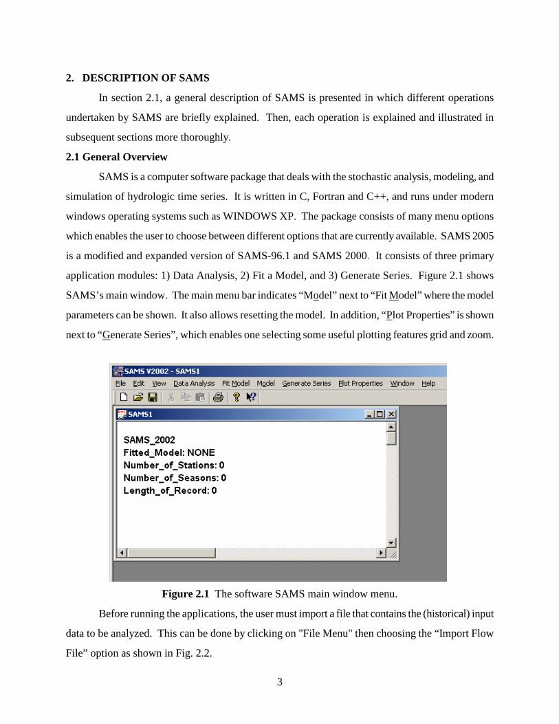
application modules: 1) Data Analysis, 2) Fit a Model, and 3) Generate Series. Figure 2.1 shows
SAMS’s main window. The main menu bar indicates “Model” next to “Fit Model” where the model
parameters can be shown. It also allows resetting the model. In addition, “Plot Properties” is shown
next to “Generate Series”, which enables one selecting some useful plotting features grid and zoom.
Figure 2.1 The software SAMS main window menu.
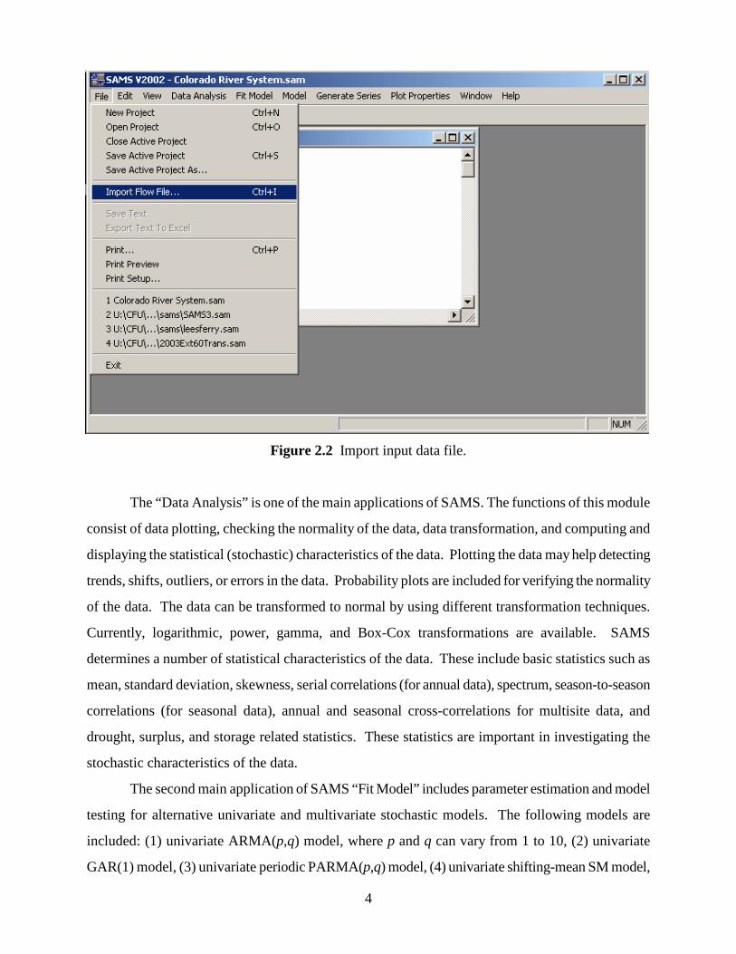
Before running the applications, the user must import a file that contains the (historical) input
data to be analyzed. This can be done by clicking on "File Menu" then choosing the “Import Flow
File” option as shown in Fig. 2.2.
4
Figure 2.2 Import input data file.
The “Data Analysis” is one of the main applications of SAMS. The functions of this module
consist of data plotting, checking the normality of the data, data transformation, and computing and
displaying the statistical (stochastic) characteristics of the data. Plotting the data may help detecting
trends, shifts, outliers, or errors in the data. Probability plots are included for verifying the normality
of the data. The data can be transformed to normal by using different transformation techniques.
Currently, logarithmic, power, gamma, and Box-Cox transformations are available. SAMS
determines a number of statistical characteristics of the data. These include basic statistics such as
mean, standard deviation, skewness, serial correlations (for annual data), spectrum, season-to-season
correlations (for seasonal data), annual and seasonal cross-correlations for multisite data, and
drought, surplus, and storage related statistics. These statistics are important in investigating the
stochastic characteristics of the data.
The second main application of SAMS “Fit Model” includes parameter estimation and model
testing for alternative univariate and multivariate stochastic models. The following models are
included: (1) univariate ARMA(p,q) model, where p and q can vary from 1 to 10, (2) univariate
GAR(1) model, (3) univariate periodic PARMA(p,q) model, (4) univariate shifting-mean SM model,

5
(5) univariate seasonal disaggregation, (6) multivariate autoregressive MAR(p) model, (7)
contemporaneous multivariate CARMA(p, q) model, where p and q can vary from 1 to 10, (8)
multivariate periodic MPAR(p) model, (9) multivariate CSM-CARMA(p, q) model, (10)
multivariate annual (spatial) disaggregation model, and (11) multivariate temporal disaggregation
model.
Two estimation methods are available, namely the method of moments (MOM) and the least
squares method (LS). MOM is available for most of the models while LS is available only for
univariate ARMA, PARMA, and CARMA models. For CARMA models, both the method of
moments (MOM) and the method of maximum likelihood (MLE) are available for estimation of the
variance-covariance (G) matrix. Regarding multivariate annual (spatial) disaggregation models,
parameter estimation is based on Valencia-Schaake or Mejia-Rousselle methods, while for annual to
seasonal (temporal) disaggregation Lane's condensed method is applied.
For stochastic simulation at several sites in a stream network system a direct modeling
approach based on multivariate autoregressive and CARMA processes are available for annual data
and multivariate periodic autoregressive process is available for seasonal data. In addition, two
schemes based on disaggregation principles are available. For this purpose, it is convenient to divide
the stations into key stations, substations, subsequent stations, etc. Generally the key stations are the
farthest downstream stations, substations are the next upstream stations, and subsequent stations are
the next further upstream stations etc. In the first scheme, the annual flows at the key stations are
added creating an annual flow data at an “artificial or index station”. Subsequently, a univariate
ARMA(p,q) model is fitted to the annual flows of the index station. Then, a spatial disaggregation
model relating the annual flows of the index station to the annual flows of the key stations is fitted.
Further, one or more statistical disaggregation models relating the annual flows of the key stations to
those of the substations are fitted. This process can be repeated as long as there are any unmodeled
stations left, where each modeled station can be defined as key station at the next disaggregation
level and each unmodeled station can be defined as substation. In the second scheme a multivariate
model is fitted to the annual data of the key stations, then the rest of the model relating the annual
flows at the key station, substations, and subsequent stations are conducted in a similar manner as in
the first scheme. Furthermore, if the objective of the modeling exercise is to generate seasonal data
by using disaggregration approaches, then an additional temporal disaggregration model is fitted that

6
relates the annual flows of a group of stations with the corresponding seasonal flows. The foregoing
schemes of modeling and generation at the annual time scale with spatial disaggregation as needed
and then performing the temporal disaggregation can also be reversed, i.e. starting with temporal
disaggregation of key station annual flows to seasonal flows followed by spatial disaggregation.
The third main application of SAMS is “Generate Series”, i.e. simulating synthetic data.
Data generation is based on the models, approaches, and schemes as mentioned above. The model
parameters for data generation are those that are estimated by SAMS. The user also has the option of
importing annual series at key stations (e.g. series generated using a software other than SAMS).
The statistical characteristics of the generated data are presented in graphical or tabular forms along
with the historical statistics of the data that was used in fitting the generating model. The generated
data including the "generated" statistics can be displayed graphically or in table form, and be printed
and/or written on specified output files. As a matter of clarification, we will summarize here the
overall data generation procedure for generating seasonal data based on scheme 2:
(a) a multivariate model, such as AR(p), is utilized to generate the annual flows at the key
stations;
(b) a spatial disaggregation model is used to disaggregate the generated annual flows at the key
stations into annual flows at the substations, followed by additional spatial disaggregations
until all upstream stations are taken into account;
(c) a temporal disaggregation model is used to disaggregate the annual flows at one or more
groups of stations into the corresponding seasonal flows at those stations.
2.2 Statistical Analysis of Data
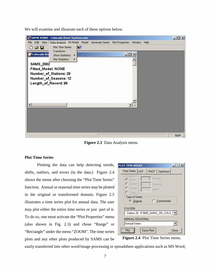
Figure 2.3 shows the “Data Analysis” menu. By selecting this menu the user can carry out
statistical analysis on the annual or seasonal data, either original or transformed data. The following
are the four operations that the user may choose:
1. Plot Time Series.
2. Transform.
3. Show Statistics.
4. Plot Statistics.
7
We will examine and illustrate each of these options below.
Figure 2.3 Data Analysis menu.
Plot Time Series
Plotting the data can help detecting trends,
shifts, outliers, and errors (in the data.) Figure 2.4
shows the menu after choosing the “Plot Time Series”
function. Annual or seasonal time series may be plotted
in the original or transformed domain. Figure 2.5
illustrates a time series plot for annual data. The user
may plot either the entire time series or just part of it.
To do so, one must activate the “Plot Properties” menu
(also shown in Fig. 2.3) and chose “Range” or
“Rectangle” under the menu “ZOOM”. The time series
plots and any other plots produced by SAMS can be
easily transferred into other word/image processing or spreadsheet applications such as MS Word,
Figure 2.4 Plot Time Series menu.
8
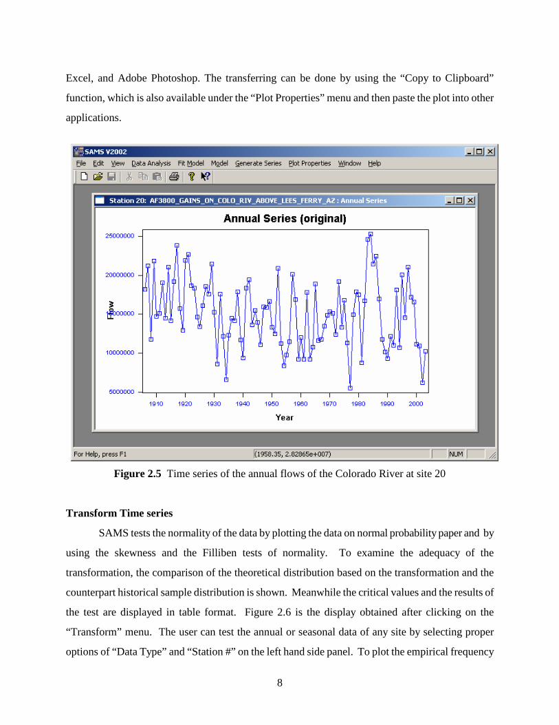
Excel, and Adobe Photoshop. The transferring can be done by using the “Copy to Clipboard”
function, which is also available under the “Plot Properties” menu and then paste the plot into other
applications.
Figure 2.5 Time series of the annual flows of the Colorado River at site 20
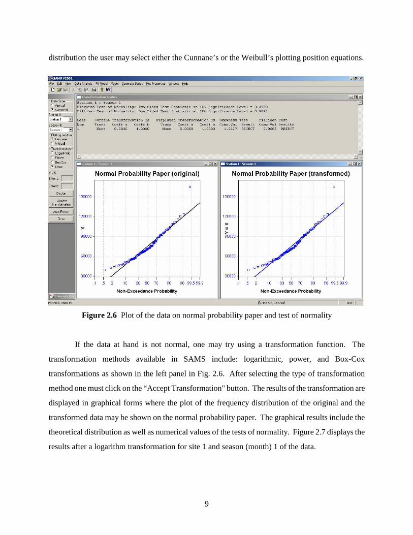
Transform Time series
SAMS tests the normality of the data by plotting the data on normal probability paper and by
using the skewness and the Filliben tests of normality. To examine the adequacy of the
transformation, the comparison of the theoretical distribution based on the transformation and the
counterpart historical sample distribution is shown. Meanwhile the critical values and the results of
the test are displayed in table format. Figure 2.6 is the display obtained after clicking on the
“Transform” menu. The user can test the annual or seasonal data of any site by selecting proper
options of “Data Type” and “Station #” on the left hand side panel. To plot the empirical frequency
9
distribution the user may select either the Cunnane’s or the Weibull’s plotting position equations.
Figure 2.6 Plot of the data on normal probability paper and test of normality
If the data at hand is not normal, one may try using a transformation function. The
transformation methods available in SAMS include: logarithmic, power, and Box-Cox
transformations as shown in the left panel in Fig. 2.6. After selecting the type of transformation
method one must click on the “Accept Transformation" button. The results of the transformation are
displayed in graphical forms where the plot of the frequency distribution of the original and the
transformed data may be shown on the normal probability paper. The graphical results include the
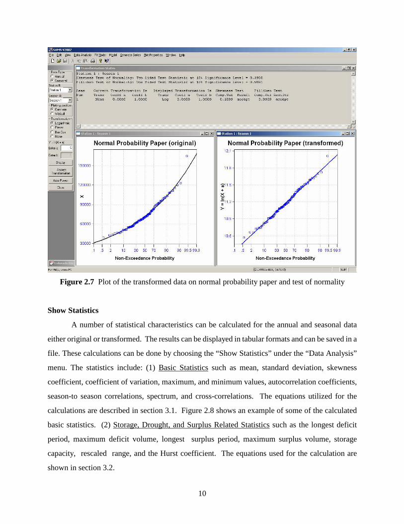
theoretical distribution as well as numerical values of the tests of normality. Figure 2.7 displays the
results after a logarithm transformation for site 1 and season (month) 1 of the data.
10
Figure 2.7 Plot of the transformed data on normal probability paper and test of normality
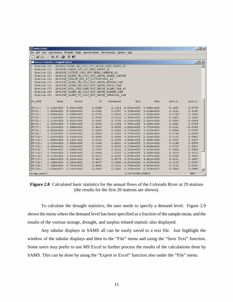
Show Statistics
A number of statistical characteristics can be calculated for the annual and seasonal data
either original or transformed. The results can be displayed in tabular formats and can be saved in a
file. These calculations can be done by choosing the “Show Statistics” under the “Data Analysis”
menu. The statistics include: (1) Basic Statistics such as mean, standard deviation, skewness
coefficient, coefficient of variation, maximum, and minimum values, autocorrelation coefficients,
season-to season correlations, spectrum, and cross-correlations. The equations utilized for the
calculations are described in section 3.1. Figure 2.8 shows an example of some of the calculated
basic statistics. (2) Storage, Drought, and Surplus Related Statistics such as the longest deficit
period, maximum deficit volume, longest surplus period, maximum surplus volume, storage
capacity, rescaled range, and the Hurst coefficient. The equations used for the calculation are
shown in section 3.2.
11
Figure 2.8 Calculated basic statistics for the annual flows of the Colorado River at 29 stations
(the results for the first 20 stations are shown).
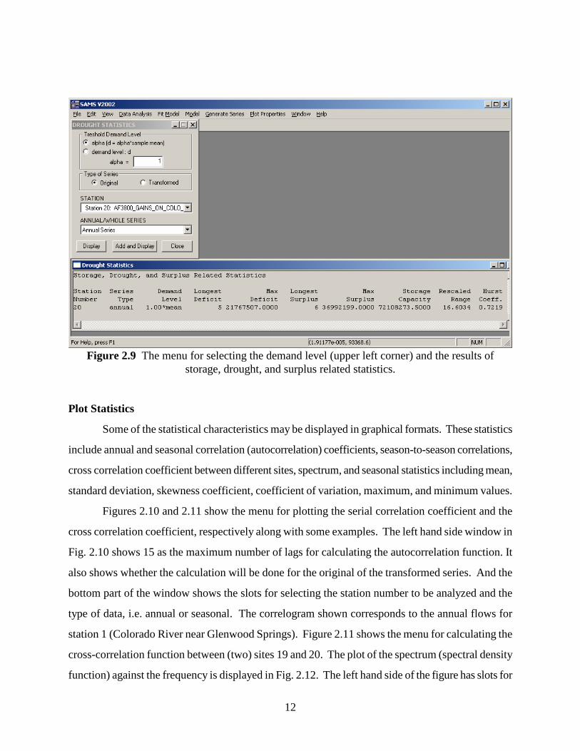
To calculate the drought statistics, the user needs to specify a demand level. Figure 2.9
shows the menu where the demand level has been specified as a fraction of the sample mean, and the
results of the various storage, drought, and surplus related statistic also displayed.
Any tabular displays in SAMS all can be easily saved to a text file. Just highlight the
window of the tabular displays and then to the “File” menu and using the “Save Text” function.
Some users may prefer to use MS Excel to further process the results of the calculations done by
SAMS. This can be done by using the “Export to Excel” function also under the “File” menu.
12
Figure 2.9 The menu for selecting the demand level (upper left corner) and the results of storage, drought, and surplus related statistics.
Plot Statistics
Some of the statistical characteristics may be displayed in graphical formats. These statistics
include annual and seasonal correlation (autocorrelation) coefficients, season-to-season correlations,
cross correlation coefficient between different sites, spectrum, and seasonal statistics including mean,
standard deviation, skewness coefficient, coefficient of variation, maximum, and minimum values.
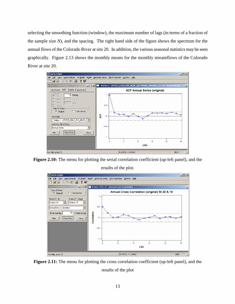
Figures 2.10 and 2.11 show the menu for plotting the serial correlation coefficient and the
cross correlation coefficient, respectively along with some examples. The left hand side window in
Fig. 2.10 shows 15 as the maximum number of lags for calculating the autocorrelation function. It
also shows whether the calculation will be done for the original of the transformed series. And the
bottom part of the window shows the slots for selecting the station number to be analyzed and the
type of data, i.e. annual or seasonal. The correlogram shown corresponds to the annual flows for
station 1 (Colorado River near Glenwood Springs). Figure 2.11 shows the menu for calculating the
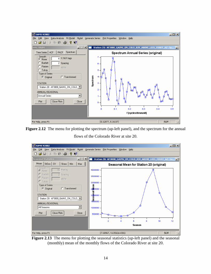
cross-correlation function between (two) sites 19 and 20. The plot of the spectrum (spectral density
function) against the frequency is displayed in Fig. 2.12. The left hand side of the figure has slots for
13
selecting the smoothing function (window), the maximum number of lags (in terms of a fraction of
the sample size N), and the spacing. The right hand side of the figure shows the spectrum for the
annual flows of the Colorado River at site 20. In addition, the various seasonal statistics may be seen
graphically. Figure 2.13 shows the monthly means for the monthly streamflows of the Colorado
River at site 20.
Figure 2.10: The menu for plotting the serial correlation coefficient (up-left panel), and the
results of the plot.
Figure 2.11: The menu for plotting the cross correlation coefficient (up-left panel), and the
results of the plot
14
Figure 2.12 The menu for plotting the spectrum (up-left panel), and the spectrum for the annual
flows of the Colorado River at site 20.
Figure 2.13 The menu for plotting the seasonal statistics (up-left panel) and the seasonal (monthly) mean of the monthly flows of the Colorado River at site 20.
15
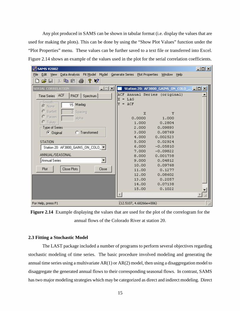
Any plot produced in SAMS can be shown in tabular format (i.e. display the values that are
used for making the plots). This can be done by using the “Show Plot Values” function under the
“Plot Properties” menu. These values can be further saved to a text file or transferred into Excel.
Figure 2.14 shows an example of the values used in the plot for the serial correlation coefficients.
Figure 2.14 Example displaying the values that are used for the plot of the correlogram for the
annual flows of the Colorado River at station 20.
2.3 Fitting a Stochastic Model
The LAST package included a number of programs to perform several objectives regarding
stochastic modeling of time series. The basic procedure involved modeling and generating the
annual time series using a multivariate AR(1) or AR(2) model, then using a disaggregation model to
disaggregate the generated annual flows to their corresponding seasonal flows. In contrast, SAMS
has two major modeling strategies which may be categorized as direct and indirect modeling. Direct

16
modeling means fitting an stationary model (e.g. univariate ARMA or multivariate AR, CARMA or
CSM-CARMA) directly to the annual data or fitting a periodic (seasonal) model (e.g. univariate
PARMA or multivariate PAR) directly to the seasonal data of the system at hand. Disaggregation
modeling, on the other hand, is an indirect procedure because the modeling of the annual data for a
site can rely on the modeling of the annual data of another site (key station), and the modeling of
seasonal data involves also modeling the corresponding annual data as well before the seasonal data
are obtained by temporal disaggregation. SAMS categorizes the models into those for the annual
data and for the seasonal data. In each category, there are univariate, multivariate, and
disaggregation models. The following specific models are currently available in SAMS under each
category:
1. For annual data:
• Univariate ARMA(p,q) model.
• Univariate GAR(1) model.
• Univariate Shifting Mean (SM) model.
• Multivariate AR(p) model (MAR).
• Contemporaneous ARMA(p,q) model (CARMA).
• CSM-CARMAR(p,q) model.
• Multivariate annual (spatial) disaggregation.
2. For seasonal data:
• Univariate PARMA(p,q) model.
• Multivariate PAR(p) model (MPAR(p)).
• Univariate seasonal disaggregation model.
• Multivariate spatial-seasonal disaggregation model.
• Multivariate seasonal-spatial disaggregation model.
The operation for fitting the models rather than a disaggregation model is basically the same.
After clicking on the “Fit Model” menu and choosing the desired model, a menu for fitting the
chosen model will appear where the site number, the model order, etc. can be specified. The user
needs to specify the station (site) number(s). If standardization of the data is desired, one must click
on the "Standardize Data" button. Generally, the modeling is performed with data in which the mean
17
is subtracted. Thus, standardization implies that not only the mean is subtracted but in addition the
data will be further transformed to have standard deviation equal to one. For example, for monthly
data the mean for month 5 is subtracted and the result is divided by the standard deviation for that
month. As a result, the mean and the standard deviation of the standardized data for month 5
become equal to zero and one, respectively. Then, the order of the model to be fitted is selected, for
instance for ARMA models, one must enter p and q. In the case of MAR or MPAR models, one
must key in the order p only. Subsequently, the method of estimation of the model parameters must
be selected.
Currently SAMS provides two methods of estimation namely the method of moments
(MOM) and the least squares (LS) method. MOM is available for the ARMA(p,q), GAR(1), SM,
MAR(p), CSM part of the CSM-CARMA, PARMA(p,1), and MPAR(p) models while LS is
available for ARMA(p,q), CARMA(p,q), and PARMA(p,q) models. The LS method is often
iterative and may require some initial parameters estimates (starting points). These starting points
are either based on fitting a high order simpler model using LS or by using the MOM parameters
estimates as starting points. For cases where the MOM estimates are not available such as for the
PARMA(p,q) model where q>1, the MOM parameter estimates of the closest model will be used
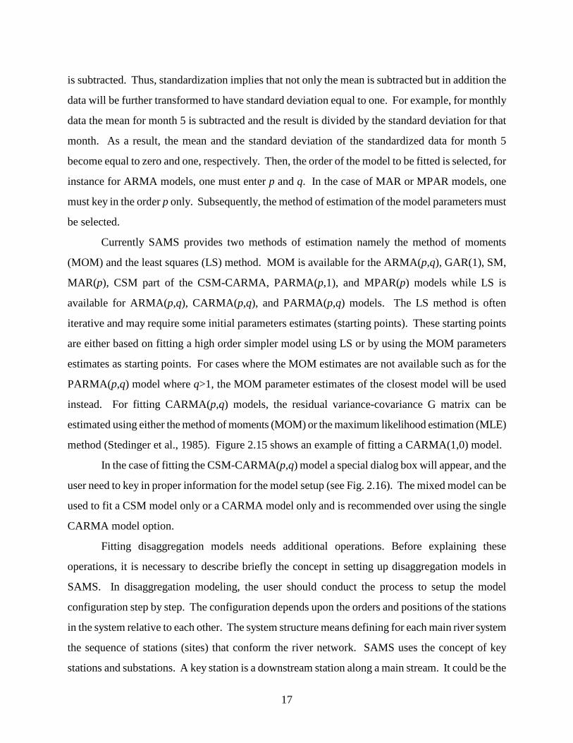
instead. For fitting CARMA(p,q) models, the residual variance-covariance G matrix can be
estimated using either the method of moments (MOM) or the maximum likelihood estimation (MLE)
method (Stedinger et al., 1985). Figure 2.15 shows an example of fitting a CARMA(1,0) model.
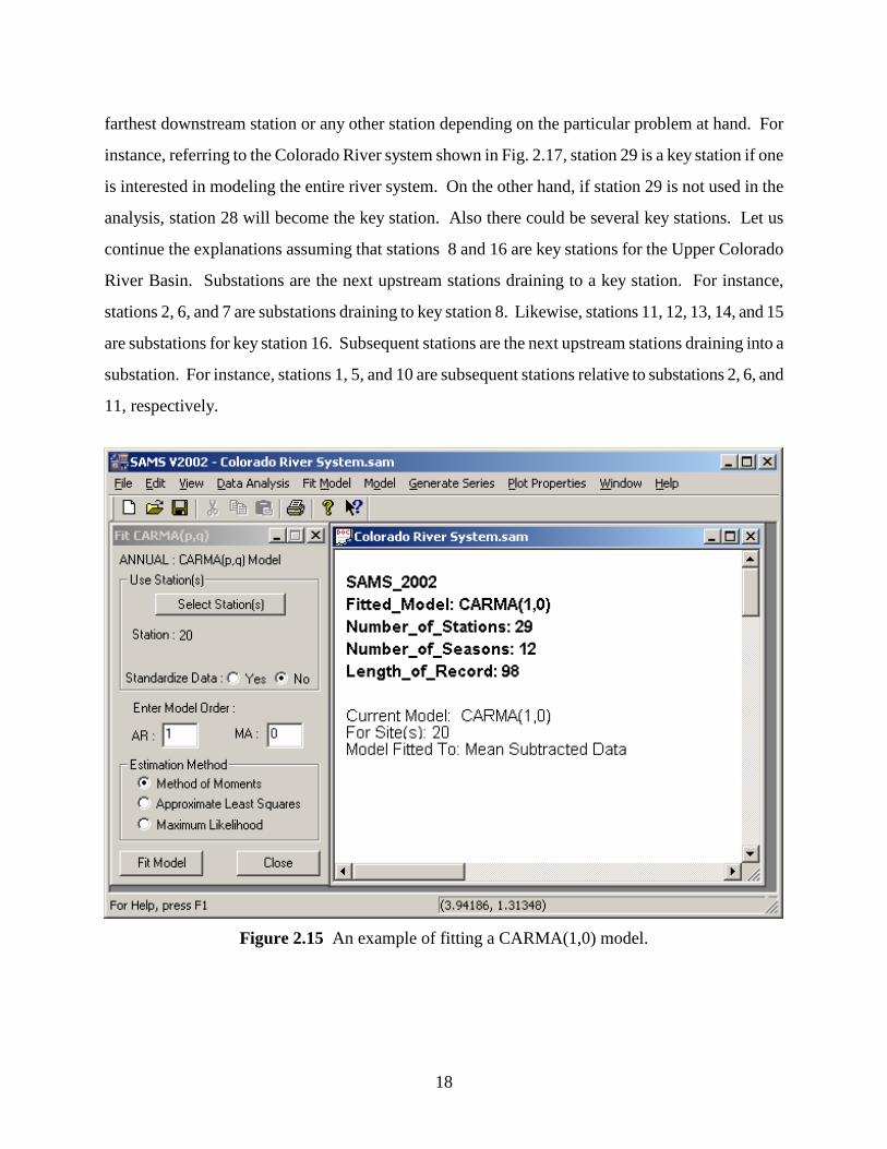
In the case of fitting the CSM-CARMA(p,q) model a special dialog box will appear, and the
user need to key in proper information for the model setup (see Fig. 2.16). The mixed model can be
used to fit a CSM model only or a CARMA model only and is recommended over using the single
CARMA model option.
Fitting disaggregation models needs additional operations. Before explaining these
operations, it is necessary to describe briefly the concept in setting up disaggregation models in
SAMS. In disaggregation modeling, the user should conduct the process to setup the model
configuration step by step. The configuration depends upon the orders and positions of the stations
in the system relative to each other. The system structure means defining for each main river system
the sequence of stations (sites) that conform the river network. SAMS uses the concept of key
stations and substations. A key station is a downstream station along a main stream. It could be the
18
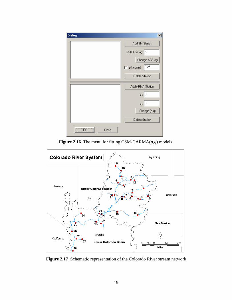
farthest downstream station or any other station depending on the particular problem at hand. For
instance, referring to the Colorado River system shown in Fig. 2.17, station 29 is a key station if one
is interested in modeling the entire river system. On the other hand, if station 29 is not used in the
analysis, station 28 will become the key station. Also there could be several key stations. Let us
continue the explanations assuming that stations 8 and 16 are key stations for the Upper Colorado
River Basin. Substations are the next upstream stations draining to a key station. For instance,
stations 2, 6, and 7 are substations draining to key station 8. Likewise, stations 11, 12, 13, 14, and 15
are substations for key station 16. Subsequent stations are the next upstream stations draining into a
substation. For instance, stations 1, 5, and 10 are subsequent stations relative to substations 2, 6, and
11, respectively.
Figure 2.15 An example of fitting a CARMA(1,0) model.
19
Figure 2.16 The menu for fitting CSM-CARMA(p,q) models.
Figure 2.17 Schematic representation of the Colorado River stream network
20
In addition, for defining a "disaggregation procedure" SAMS uses the concept of groups. A
group consists of one or more key stations and their corresponding substations. Groups must be
defined in each disaggregation step. Each group contains a certain number of stations to be modeled
in a multivariate fashion, i.e. jointly, in order to preserve their cross-correlations. For instance, if a
certain group has two key stations and three substations, then the disaggregation process will
preserve the cross-correlations between all stations (key and substations.) On the other hand, if two
separate groups are selected, then the cross-correlations between the stations that belong to the same
group will be preserved, but the cross-correlations between stations belonging to different groups
will not be preserved.
The definition of a group is important in the disaggregation process. For instance, referring
to Fig. 2.17, key station 8 and substations 2, 6, and 7 may form one group in which the flows of all
these stations are modeled jointly in a multivariate framework, while key station 16 and its
substations 11, 12, 13, 14, and 15 may form another group. In this case, the cross-correlations
between the stations within each group will be preserved but the cross-correlations among stations of
the two different groups will not be preserved. For example, the cross-correlations between stations
8 and 16 will not be preserved but the cross-correlations between stations 8 and 2 will be preserved.
On the other hand, if all the stations are defined in a single group, then the cross-correlations
between all the stations will be preserved. After modeling and generating the annual flows at the
desired stations, the annual flows can be disaggregated into seasonal flows. This is handled again by
using the concept of groups as explained above. The user, for example, may choose stations 11, 12,
13, 14, 15, and 16 as one group. Then, the annual flows for these stations may be disaggregated into
seasonal flows by a multivariate disaggregation model so as to preserve the seasonal cross-
correlations between all the stations.
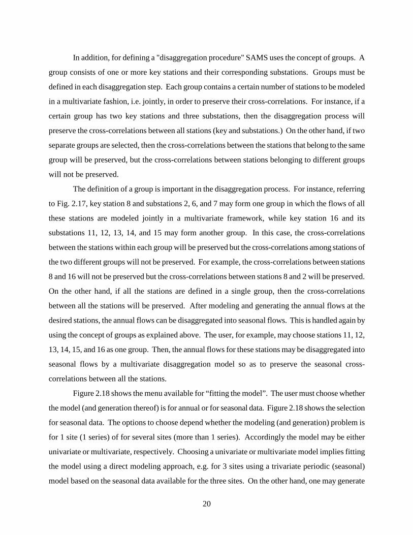
Figure 2.18 shows the menu available for “fitting the model”. The user must choose whether
the model (and generation thereof) is for annual or for seasonal data. Figure 2.18 shows the selection
for seasonal data. The options to choose depend whether the modeling (and generation) problem is
for 1 site (1 series) of for several sites (more than 1 series). Accordingly the model may be either
univariate or multivariate, respectively. Choosing a univariate or multivariate model implies fitting
the model using a direct modeling approach, e.g. for 3 sites using a trivariate periodic (seasonal)
model based on the seasonal data available for the three sites. On the other hand, one may generate
21
seasonal flows indirectly using aggregation and disaggregation methods. When using disaggregation
methods two broad options are available (Fig. 2.18), i.e. spatial-seasonal and seasonal-spatial. The
first option defines a modeling approach whereby annual flow are generated first at key stations,
subsequently, spatial disaggregation is applied to generate annual flows at upstream stations, then
seasonal flow are obtained using temporal disaggregation. Alternatively, the second option defines a
modeling approach where annual flows are generated at key stations, which are then disaggregated
into seasonal flows based on temporal disaggregation models. And the final step is to disaggregate
such seasonal flows spatially to obtain the seasonal flows at all stations in the system at hand.
Figure 2.18 The menu for model fitting. Note that “seasonal data” and “disaggregation” options
are selected (highlighted) and the options “Spatial-temporal” and “Temporal-Spatial” are shown.
SAMS has two schemes for modeling the key stations. In the first scheme, denoted as
Scheme 1, the annual flows of the key stations that belong to a given group are aggregated to form an
“index station”, then a univariate ARMA(p,q) model is used to model the aggregated flows (of the
index station.) The aggregated annual flows are then disaggregated (spatially) back to each key
station by using the Valencia and Schaake or the Mejia and Rouselle disagregation methods. Then
the annual flows at the key stations are disaggregated spatially to obtain the annual flows at the
substations and then to the subsequent stations, etc. The second scheme, denoted as Scheme 2, uses

22
a multivariate model to represent (generate) the annual flows of the key stations belonging to a given
group and then disaggregate those flows spatially to obtain the annual flows for the substations,
subsequent stations, etc. For either Scheme 1 or 2, temporal disaggregation may be carried out if
seasonal flows are desired. The mathematical description of the disaggregation methods is presented
in chapter 4, and examples of disaggregation modeling applied to real streamflow data are presented
in chapter 5.
In applying disaggregation methods the user needs to choose the specific disaggregation
models for both spatial and temporal disaggregation. For example, when modeling seasonal data the
user may select either the “spatial-temporal” or the “temporal-spatial” option. In any selection one
must determine the type of disaggregation models. Figure 2.19 shows the windows option after
choosing the “spatial-temporal” option. The modeling scheme as either 1 or 2 (as noted above) must
model) be chosen, as well as the type of spatial disaggregation (either the Valencia-Schaake or
Mejia-Rousselle model) and the type of temporal disaggregation (for this purpose only Lane’s model
is available). The option “Temporal-Spatial” is slightly different where the user has a choice
between two temporal disaggregation models, namely Lane’s model and Grygier and Stedinger
model.
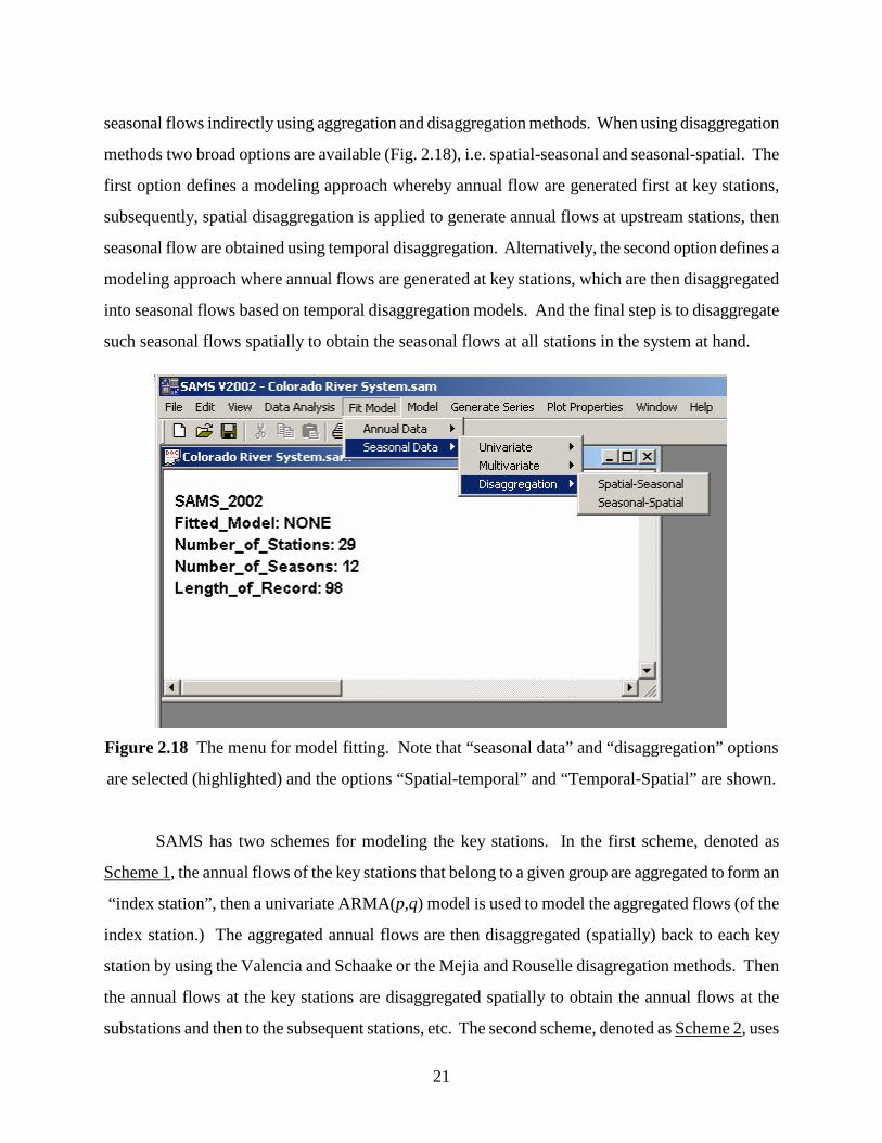
As illustration some of the steps and options followed in using a disaggregation approach are
shown in Figs. 2.19 to 2.23. They are summarized as:
• In Fig. 2.19 Scheme 1 is selected along with the V-S model for spatial disaggregation and
Lane’s model for temporal disaggregation.
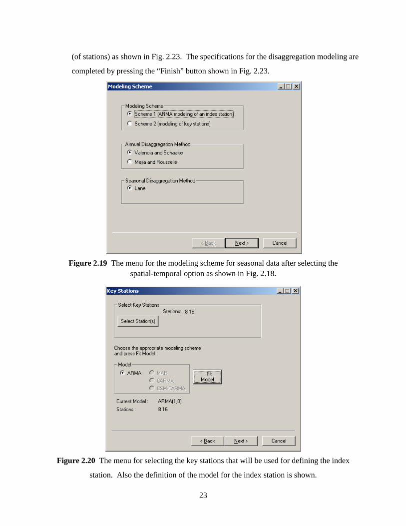
• In Fig. 2.20 stations 8 and 16 (refer to Fig. 2.17) are selected as key stations and an index
station will be formed (the aggregation of he annual flows for sites 8 and 16). Then the
ARMA(1,0) model was chosen to generate the annual flows of the index station.
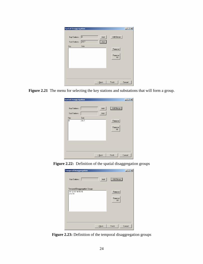
• The spatial disaggregation of the annual flows for key to substations must be carried our by
groups. For example, this could be accomplished by considering key station 8 and 16 and
their corresponding substations 2, 6, and 7 and 11, 12, 13, 14, and 15, respectively into a
single group or by forming two or more groups. For instance, 2 groups were formed one per
key station and Figs. 2.21 and 2.22 show the procedure for selecting the group corresponding
to key station 8.
• The temporal disaggregation (from annual into seasonal flows) is also performed by groups
23
(of stations) as shown in Fig. 2.23. The specifications for the disaggregation modeling are
completed by pressing the “Finish” button shown in Fig. 2.23.
Figure 2.19 The menu for the modeling scheme for seasonal data after selecting the spatial-temporal option as shown in Fig. 2.18.
Figure 2.20 The menu for selecting the key stations that will be used for defining the index
station. Also the definition of the model for the index station is shown.
24
Figure 2.21 The menu for selecting the key stations and substations that will form a group.
Figure 2.22: Definition of the spatial disaggregation groups
Figure 2.23: Definition of the temporal disaggregation groups
25
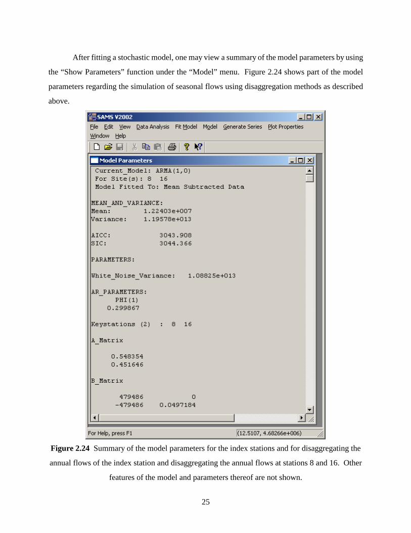
After fitting a stochastic model, one may view a summary of the model parameters by using
the “Show Parameters” function under the “Model” menu. Figure 2.24 shows part of the model
parameters regarding the simulation of seasonal flows using disaggregation methods as described
above.
Figure 2.24 Summary of the model parameters for the index stations and for disaggregating the
annual flows of the index station and disaggregating the annual flows at stations 8 and 16. Other
features of the model and parameters thereof are not shown.
26
2.4 Generating Synthetic Series
Data generation is an important subject in stochastic hydrology and has received a lot of
attention in hydrologic literature. Data generation is used by hydrologists for many purposes. These
include, for example, reservoir sizing, planning and management of an existing reservoir, and
reliability of a water resources system such as a water supply or irrigation system (Salas et al,1980).
Stochastic data generation can aid in making key management decisions especially in critical
situations such as extended droughts periods (Frevert et al, 1989). The main philosophy behind
synthetic data generation is that synthetic samples are generated which preserve certain statistical
properties that exist in the natural hydrologic process (Lane and Frevert, 1990). As a result, each
generated sample and the historic sample are equally likely to occur in the future. The historic
sample is not more likely to occur than any of the generated samples (Lane and Frevert, 1990).
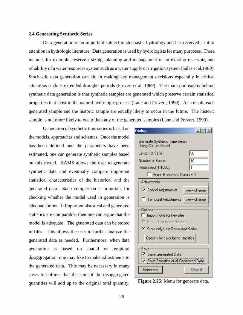
Generation of synthetic time series is based on
the models, approaches and schemes. Once the model
has been defined and the parameters have been
estimated, one can generate synthetic samples based
on this model. SAMS allows the user to generate
synthetic data and eventually compare important
statistical characteristics of the historical and the
generated data. Such comparison is important for
checking whether the model used in generation is
adequate or not. If important historical and generated
statistics are comparable, then one can argue that the
model is adequate. The generated data can be stored
in files. This allows the user to further analyze the
generated data as needed. Furthermore, when data
generation is based on spatial or temporal
disaggregation, one may like to make adjustments to
the generated data. This may be necessary in many
cases to enforce that the sum of the disaggregated
quantities will add up to the original total quantity.
Figure 2.25: Menu for generate data.
27
For example, spatial adjustments may be necessary if the annual flows at a key station is exactly the
sum of the annual flows at the corresponding substations. Likewise, in the case of temporal
disaggregation, one may like to assure that the sum of monthly values will add up to the annual
value. Various options of adjustments are included in SAMS. Further descriptions on spatial and
temporal adjustments are described in later sections of this manual.
Figure 2.25 shows the data generation menu. In this menu the user must specify necessary
information for the generation process. For example, the length of the generated data, how many
samples will be generated, and whether the generated data or the statistics of the generated data will
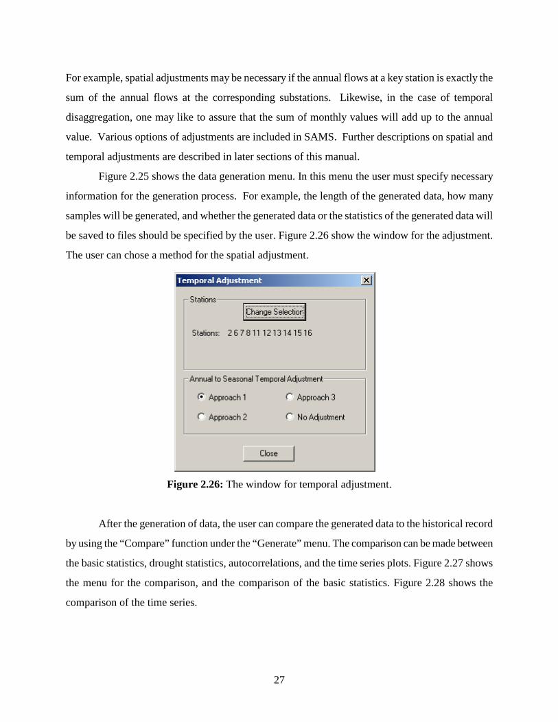
be saved to files should be specified by the user. Figure 2.26 show the window for the adjustment.
The user can chose a method for the spatial adjustment.
Figure 2.26: The window for temporal adjustment.
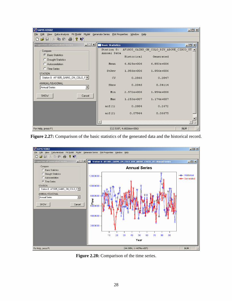
After the generation of data, the user can compare the generated data to the historical record
by using the “Compare” function under the “Generate” menu. The comparison can be made between
the basic statistics, drought statistics, autocorrelations, and the time series plots. Figure 2.27 shows
the menu for the comparison, and the comparison of the basic statistics. Figure 2.28 shows the
comparison of the time series.
28
Figure 2.27: Comparison of the basic statistics of the generated data and the historical record.
Figure 2.28: Comparison of the time series.
29
3 DEFINITION OF STATISTICAL CHARACTERISTICS
A time series process can be characterized by a number of statistical properties such as the
mean, standard deviation, coefficient of variation, skewness coefficient, season-to-season
correlations, autocorrelations, cross-correlations, and storage and drought related statistics. These
statistics are defined for both annual and seasonal data as shown below.
3.1 Basic Statistics
3.1.1 Annual Data
The mean and the standard deviation of a time series yt are estimated by
∑=
=N
tty
Ny
1
1 (3.1)
and
∑=
−=N
tt yy
Ns
1
2)(1
(3.2)
respectively, where N is the sample size. The coefficient of variation is defined as yscv /= .
Likewise, the skewness coefficient is estimated by
3
1
3)(1
s
yyN
g
N
tt∑
=−
= (3.3)
The sample autocorrelation coefficients rk of a time series may be estimated by
0m
mr kk = (3.4)
where
∑−
=+ −−=
kN
ttktk yyyy
Nm
1
))((1
(3.5)
and k = time lag. Likewise, for multisite series, the lag-k sample cross-correlations between site i
and site j, denoted by rkij , may be estimated by
jjii
ijkij
kmm
mr
00
= (3.6)
where
30
∑−
=+ −−=
kN
t
jjt
iikt
ijk yyyy
Nm
1
)()()()( ))((1
(3.7)
in which iim0 is the sample variance for site i.
3.1.2 Seasonal data
Seasonal hydrologic time series, such as monthly flows, are better characterized by seasonal
statistics. Let yν,τ be a seasonal time series, where ν = 1,...,N represents years with N being the
number of years, and τ = 1,...,ω seasons with ω being the number of seasons. The mean and standard
deviation for season τ can be estimated by
∑=
=N
yN
y1
,1
ντντ (3.8)
and
∑=
−=N
yyN
s1
2, )(
1
νττντ (3.9)
respectively. The seasonal coefficient of variation is τττ yscv /= . Similarly, the seasonal skewness
coefficient is estimated by
3
1
3, )(
1
τ
νττν
τs
yyN
g
N
∑=
−= (3.10)
The sample lag-k season-to-season correlation coefficient may be estimated by
k
kk
mm
mr
−
=ττ
ττ
,0,0
,, (3.11)
where
∑=
−− −−=N
kkk yyyyN
m1
,,, ))((1
νττνττντ (3.12)
in which τ,0m represents the sample variance for season τ. Likewise, for multisite series,
the lag-k sample cross-correlations between site i and site j, for season τ, ijkr τ, may be estimated by
jj
kii
ijkij
kmm
mr
−
=ττ
ττ
,0,0
,, (3.13)
and
31
∑=
−− −−=N
jjk
iiijk yyyy
Nm
1
)()(,
)()(,, ))((
1
νττνττντ (3.14)
in which iim τ,0 represents the sample variance for season τ and site i. Note that in Eqs. (3.11) through
(3.14) when τ - k < 1 τ − <k 1 , the terms, )()(,,0, ,,,,,1 j
kj
kkkk yymyy −−−−−= ττντττνν , and jjkm −τ,0 are
replaced by )()(,,0,1 ,,,,,2 j
kj
kkkk yymyy −+−+−+−+−+−= τωτωντωτωτωνν , and jjkm −+τω,0 , respectively.
3.2 Storage, Drought, and Surplus Related Statistics
3.2.1 Storage Related Statistics
The storage-related statistics are particularly important in modeling time series for simulation
studies of reservoir systems. Such characteristics are generally functions of the variance and
autocovariance structure of a time series. Consider the time series yi , i = 1, ..., N and a subsample y1
, ..., yn with n ≤ N. Form the sequence of partial sums Si as
niyySS niii ,,1,)(1 K=−+= − (3.15)
where S0 = 0 and ny is the sample mean of y1 , ..., yn which is determined by Eq. (3.1). Then, the
adjusted range *nR and the rescaled adjusted range *nR can be calculated by
),,,min(),,,max( 1010*
nnn SSSSSSR KK −= (3.16)
and
n
nn s
RR
*** = (3.17)
respectively, in which sn is the standard deviation of y1 , ..., yn which is determined by Eq. (3.2).
Likewise, the Hurst coefficient for a series is estimated by
2,)2/ln(
)ln( **
>= nn
RK n (3.18)
The calculation of the storage capacity is based on the sequent peak algorithm (Loucks, et al.,
1981) which is equivalent to the Rippl mass curve method. The algorithm, applied to the time series
yi , i = 1, ..., N may be described as follows. Based on yi and the demand level d, a new
sequence 'iS can be determined as
32
−+= −
otherwise
posititiveifydSS ii
i0
'1' (3.19)
where 0'0 =S . Then the storage capacity is obtained as
),,max( ''1 Nc SSS K= (3.20)
Note that algorithms described in Eqs.(3.15) to (3.20) apply also to seasonal series. In this
case, the underlying seasonal series τν ,y is simply denoted as ty .
3.2.2 Drought Related Statistics
The drought-related statistics are also important in modeling hydrologic time series (Salas,
1993). For the series yi , i = 1, ..., N, the demand level d may be defined as 10, <<⋅ αα y (for
example, for yd == ,1α ). A deficit occurs when yi < d consecutively during one or more years
until yi > d again. Such a deficit can be defined by its duration L, by its magnitude M, and by its
intensity I = M/L. Assume that m deficits occur in a given hydrologic sample, then the maximum
deficit duration (longest drought or maximum run-length) is given by
),,max( 1*
mn LLL K= (3.21)
and the maximum deficit magnitude (maximum run-sum) is defined by
),,max( 1*
mn MMM K= (3.22)
In SAMS, the longest drought duration and the maximum deficit magnitude are estimated for both
annual and seasonal series.
3.2.3 Surplus Related Statistics
For our purpose here, surplus related statistics are simply the opposite of drought related
statistics. Considering the same threshold level d, a surplus occurs when yi > d consecutively until yi
< d again. Then, assuming that m surpluses occur during a given time period N, the maximum
surplus period L* and maximum surplus magnitude M* may be determined also from Eqs. (3.21) and
(3.22).
33
4 MATHEMATICFAL MODELS
The following univariate and multivariate models are available in SAMS for modeling of
annual and seasonal data.
1. For Annual Modeling:
• Univariate ARMA(p,q) model.
• Univariate GAR(1) model.
• SM (shifting mean) model.
• Multivariate AR(p) model (MAR).
• Contemporaneous ARMA(p,q) model (CARMA(p,q)).
• Mixture of contemporaneous shifting mean and ARMA(p,q) models (CSM
– CARMA(p,q)).
2. For Seasonal Modeling:
• Univariate PARMA(p,q) model.
• Multivariate PAR(p) model (MPAR).
3. Disaggregation Models
• Spatial Valencia and Schaake.
• Spatial Mejia and Rousselle.
• Temporal Lane.
• Temporal Grygier and Stedinger.
All models, except the GAR(1), assume that the underlying data is normally distributed. The
GAR(1) model assumes that the process being modeled follows a gamma distribution. Thus for all
other models than the GAR(1) it is necessary to transform the data into normal.
4.1 Data Transformations and Scaling
In cases where the normality tests in SAMS indicate that the observed series are not normally
distributed, the data has to be transformed into normal before applying the models. To normalize the
data, the following transformations Y = f(X) are available in SAMS:
Logarithmic
34
)ln( aXY += (4.1)
Gamma
)(XGammaY = (4.2)
Power
baXY )( += (4.3)
Box-Cox
0,1)( ≠−+= b
b
aXY
b
(4.4)
where Y is the normalized series, X is the original observed series, and a and b are transformation
coefficients. The variables Y and X represent either annual or seasonal data, where for seasonal data a
and b vary with the season. Note that the logarithmic transformation is simply the limiting form of
the Box-Cox transform as the coefficient b approaches zero. Also, the power transformation is a
shifted and scaled form of the Box-Cox transform.
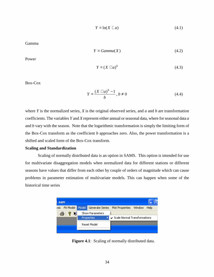
Scaling and Standardization
Scaling of normally distributed data is an option in SAMS. This option is intended for use
for multivariate disaggregation models when normalized data for different stations or different
seasons have values that differ from each other by couple of orders of magnitude which can cause
problems in parameter estimation of multivariate models. This can happen when some of the
historical time series
Figure 4.1: Scaling of normally distributed data.
35
are normally distributed and do not need to be transformed to normal while others do. To use this
option select “Scale Normal Transformations” from the SAMS menu as is illustrated in Fig. 4.1. If
this option is selected than all time series that have not been transformed by any of the
transformations in Eqs. (4.1)-(4.4) are scaled by dividing by the standard deviation.
In addition, for most of the univariate and multivariate models (except disaggregation models
and the CSM-CARMA) the normalized data can then be standardized by subtracting the mean and
dividing by the standard deviation. This option is usually offered in the model estimation dialogs in
SAMS. For example, for seasonal series, the standardization may be expressed as:
)(
,, XS
XXY
τ
ττντν
−= (4.5)
where τν ,Y is the scaled normally distributed variable with standard deviation one and mean zero
for year ν of the seasonal series for season τ. )(XSτ
and τX are the mean and the standard deviation of
the transformed series for month τ.
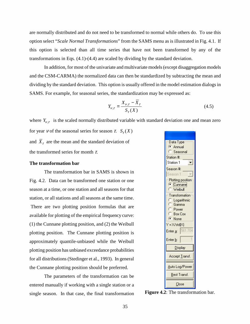
The transformation bar
The transformation bar in SAMS is shown in
Fig. 4.2. Data can be transformed one station or one
season at a time, or one station and all seasons for that
station, or all stations and all seasons at the same time.
There are two plotting position formulas that are
available for plotting of the empirical frequency curve:
(1) the Cunnane plotting position, and (2) the Weibull
plotting position. The Cunnane plotting position is
approximately quantile-unbiased while the Weibull
plotting position has unbiased exceedance probabilities
for all distributions (Stedinger et al., 1993). In general
the Cunnane plotting position should be preferred.
The parameters of the transformation can be
entered manually if working with a single station or a
single season. In that case, the final transformation
Figure 4.2: The transformation bar.
36
must be accepted by pressing on the “Accept Transf” button. The functionality of the buttons on the
transformation bar are as follows:
Display Displays the currently defined transformation.
Accept Transf Accepts the currently displayed transformation.
Auto Log/Power Searches for the best Log or Power transformation for multiple stations
and/or seasons.
Best Transf Searches for the best overall transformation for multiple stations and/or seasons
Refer to Appendix A for further information on how SAMS selects between different
transformations. There are various tests for normality available in the literature. In SAMS two
normality tests are available, namely the skewness test of normality (Salas et al., 1980; Snedecor and
Cochran, 1980) and Filliben probability plot correlation test (Filliben, 1975). These two test are
described in Appendix A.
Generation
During generation, synthetic time series are generated in the transformed domains, and
then brought into the original domain using an inverse transformation X = f-1(Y).
4.2 Univariate Models
Various univariate models are available in SAMS. The annual models are the traditional
ARMA(p,q) for modeling of autoregressive moving average processes, the GAR(1) for modeling of
gamma distributed process, the SM for modeling of processes having a shifting pattern in the mean,
and the PARMA(p,q) for modeling of seasonal processes.
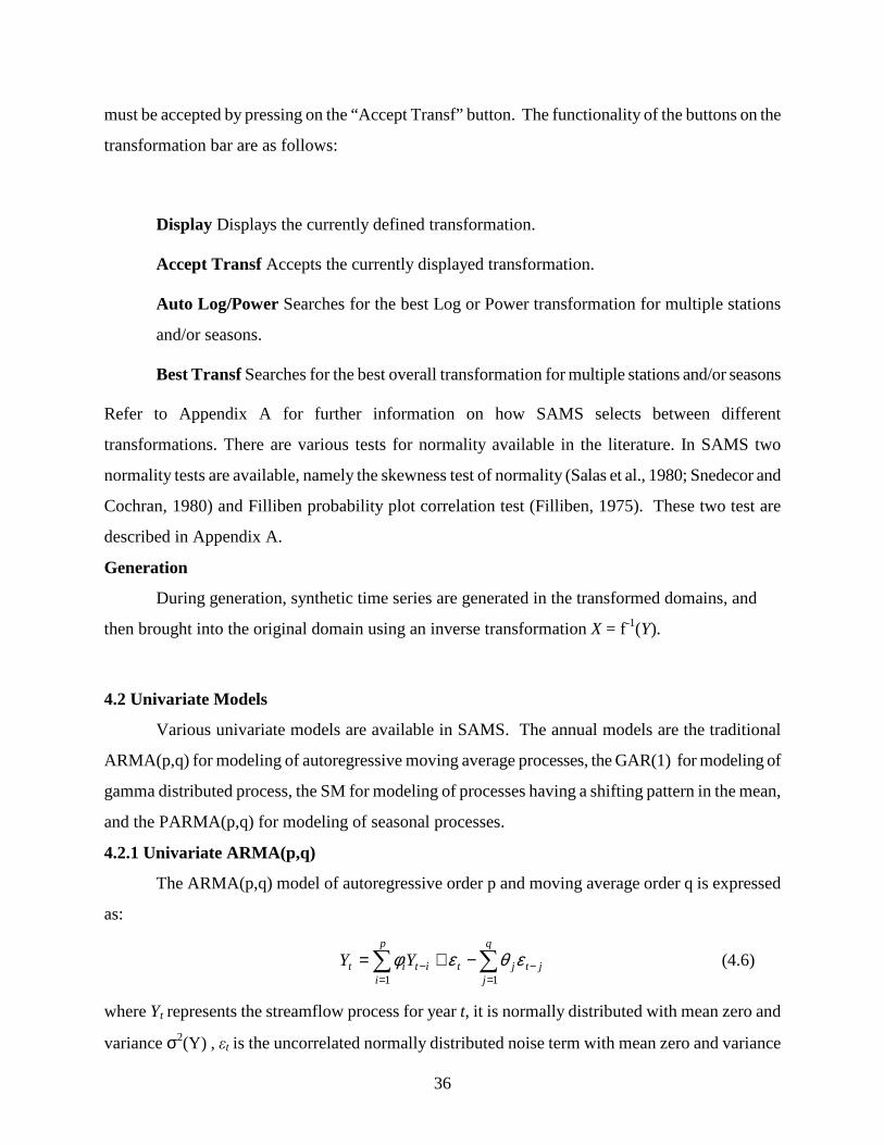
4.2.1 Univariate ARMA(p,q)
The ARMA(p,q) model of autoregressive order p and moving average order q is expressed
as:
∑∑=
−=
− −+=q
jjtjt
p
iitit YY
11
εθεφ (4.6)
where Yt represents the streamflow process for year t, it is normally distributed with mean zero and
variance σ2(Y) , εt is the uncorrelated normally distributed noise term with mean zero and variance
37
σ2(ε), {φ1,…,φp} are the autoregressive parameters and {θ1,…, θq} are the moving average
parameters. The characteristics of the autocorrelation function (ACF) and the partial autocorrelation
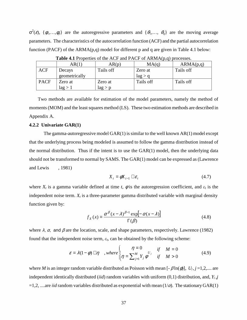
function (PACF) of the ARMA(p,q) model for different p and q are given in Table 4.1 below:
Table 4.1 Properties of the ACF and PACF of ARMA(p,q) processes. AR(1) AR(p) MA(q) ARMA(p,q)
ACF Decays geometrically
Tails off
Zero at lag > q
Tails off
PACF Zero at lag > 1
Zero at lag > p
Tails off
Tails off
Two methods are available for estimation of the model parameters, namely the method of
moments (MOM) and the least squares method (LS). These two estimation methods are described in
Appendix A.
4.2.2 Univariate GAR(1)
The gamma-autoregressive model GAR(1) is similar to the well known AR(1) model except
that the underlying process being modeled is assumed to follow the gamma distribution instead of
the normal distribution. Thus if the intent is to use the GAR(1) model, then the underlying data
should not be transformed to normal by SAMS. The GAR(1) model can be expressed as (Lawrence
and Lewis , 1981)
ttt XX εφ += −1 (4.7)
where Xt is a gamma variable defined at time t, φ is the autoregression coefficient, and εt is the
independent noise term. Xt is a three-parameter gamma distributed variable with marginal density
function given by:
[ ]
)(
)(exp)()(
1
βλαλα ββ
Γ−−−=
− xxxf X (4.8)
where λ, α, and β are the location, scale, and shape parameters, respectively. Lawrence (1982)
found that the independent noise term, εt, can be obtained by the following scheme:
0
00,)1(
1>=
=
=+−=
∑ = M
M
if
if
Ywhere jUM
j j φηη
ηφλε (4.9)
where M is an integer random variable distributed as Poisson with mean [- β ln(φ)], Uj , j =1,2,.... are
independent identically distributed (iid) random variables with uniform (0,1) distribution, and, Yj ,j
=1,2, ....are iid random variables distributed as exponential with mean (1/α). The stationary GAR(1)
38
process of Eq. (4.7) has four parameters, namely {φ, λ, α, β}. The model parameters are estimated
based on a procedure suggested by Fernandez and Salas (1990), as illustrated in Appendix A.
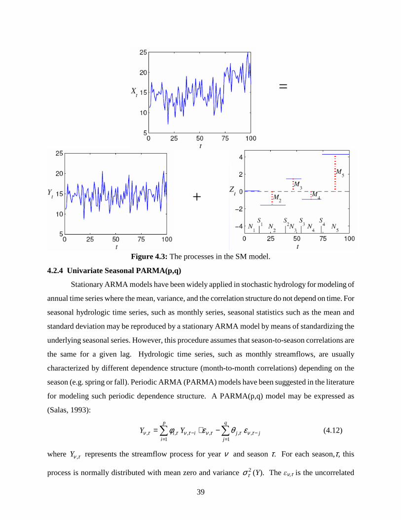
4.2.3 Univariate SM
The shifting mean (SM) model is characterized by sudden shifts or jumps in the mean. More
precisely, the underlying process is assumed to be characterized by multiple stationary states, which
only differ from each other by having different means that vary around the long term mean of the
process. The process is autocorrelated, where the autocorrelation arises only from the sudden
shifting pattern in the mean. A general definition of the SM model is given by (Sveinsson et al.,
2003 and 2005)
ttt ZYX += (4.10)
where {Xt} is a sequence of random variables representing the hydrologic process of interest; {Yt} is
a sequence of iid random variables normally distributed with mean Yµ and variance 2Yσ ; and {Zt} is
a sequence with mean zero and variance 2Zσ . The sequences {Yt} and {Zt} are assumed to be
mutually independent of each other. The Xt process is characterized by multiple “stationary” states
each of random length Ni, i = 1,2,... as shown in Fig. 4.3. The Zt process represents the shifting
pattern from one state to another, and the different states are referred to as noise levels. The noise
level process { }tZ can be written as
( ]∑=
−=
t
iSSit tIMZ
ii1
, )(1
(4.11)
Where { } ( )221 ,0N~ ZMii iidM σσ =∞
= , ii NNNS +++= L21 with 00 =S , and )(),( tI ba is the
indicator function equal to one if ),( bat ∈ and zero otherwise. The { }∞=1itN is a discrete, stationary,
delayed-renewal sequence on the positive integers, with { } )(Geometric Positive~1 piidN it∞=
(Sveinsson et al., 2003 and 2005). Thus the average length of each state of the process is the inverse
of the parameter of the positive Geometric distribution or 1/p. The estimation of model parameters
is described in Appendix A.
39
Figure 4.3: The processes in the SM model.
4.2.4 Univariate Seasonal PARMA(p,q)
Stationary ARMA models have been widely applied in stochastic hydrology for modeling of
annual time series where the mean, variance, and the correlation structure do not depend on time. For
seasonal hydrologic time series, such as monthly series, seasonal statistics such as the mean and
standard deviation may be reproduced by a stationary ARMA model by means of standardizing the
underlying seasonal series. However, this procedure assumes that season-to-season correlations are
the same for a given lag. Hydrologic time series, such as monthly streamflows, are usually
characterized by different dependence structure (month-to-month correlations) depending on the
season (e.g. spring or fall). Periodic ARMA (PARMA) models have been suggested in the literature
for modeling such periodic dependence structure. A PARMA(p,q) model may be expressed as
(Salas, 1993):
∑∑=
−=
− −+=q
jjj
p
iii YY
1,,,
1,,, τνττντνττν εθεφ (4.12)
where τν ,Y represents the streamflow process for year ν and season τ. For each season,τ, this
process is normally distributed with mean zero and variance 2τσ (Y). The εν,τ is the uncorrelated
=
+
40
noise term which for each season is normally distributed with mean zero and variance 2τσ ( ε). The
{ φ1,τ,…,φp,τ} are the periodic autoregressive parameters and the {θ1,τ,…, θq,τ} are the periodic
moving average parameters. If the number of seasons or the period is ω, then a PARMA(p,q) model
consists of ω number of individual ARMA(p,q) models, where the dependence is across seasons
instead of years. Parameters are estimated using MOM or LS as illustrated in Appendix A. The
MOM method can only be used in SAMS for q = 0 or 1.
4.3 Multivariate Models
Analysis and modeling of multiple time series is often needed in Hydrology. In SAMS full
multivariate model are available for modeling complex dependence structure in space and time at
multiple lags. Also in SAMS, contemporaneous models are available for preserving complex
dependence structure within each site but simpler structure in space across sites. Typical property of
contemporaneous models is diagonal parameter matrixes which simplify the parameters estimation
by allowing the model to be decoupled into univariate models. The multivariate models available in
SAMS are the multivariate autoregressive model MAR(p), the contemporaneous ARMA(p,q) model
dubbed as CARMA(p,q), the mixed contemporaneous shifting mean and CARMA(p,q) model
dubbed as CSM-CARMA(p,q), and the seasonal multivariate periodic autoregressive model
MPAR(p).
4.3.1 Multivariate MAR(p)
The multivariate MAR(p) model for n sites can be expressed as:
t
p
iitit εYY +Φ=∑
=−
1
(4.13)
where Y t is a n ×1 column vector of normally distributed zero mean elements )(ktY , nk ,,2,1 K= ,
representing the different sites. pΦΦΦ ,,, 21 K are the n × n autoregressive parameter matrixes, and
( )G0ε ,MVN~}{ iidt is the n ×1 vector of normally distributed noise terms with mean zero and
variance-covariance matrix G. The noise vector is independent in time and correlated in space at lag
zero. In SAMS the following notation is used to simplify the generation process:
tt zBε = (4.14)
where ( )I0z ,MVN~}{ iidt , that is a n ×1 vector of independent standard normally distributed
41
variables uncorrelated in both time and space. The n × n matrix B is a lower triangular matrix such
that G = BBT, where B is the Cholesky decomposition of G. The lag 0 spatial correlation across all
sites is preserved through the matrix B. In the MAR(p) model the correlation in time and space
across all sites is preserved up to lag p. Fur further information on parameter estimation and
generation refer to Appendix A.
4.3.2 Multivariate CARMA(p,q)
When modeling multivariate hydrologic processes based on the full multivariate ARMA
model, often problems arise in parameter estimation. The CARMA (Contemporaneous
Autoregressive Moving Average) model was suggested as a simpler alternative to the full
multivariate ARMA model (Salas, et al., 1980). In the CARMA(p,q) model, both autoregressive and
moving average parameter matrixes are assumed to be diagonal such that a multivariate model can
be decoupled into univariate ARMA models. Thus, instead of estimating the model parameters
jointly, they can be estimated independently for each single site by regular univariate ARMA model
estimation procedures. This allows for identification of the best univariate ARMA model for each
single station. Thus different dependence structure in time can be modeled for each site, instead of
having to assume a similar dependence structure in time for all sites if a full multivariate ARMA
model was used.
The CARMA(p,q) model for n sites can be expressed as:
∑∑=
−=
− Θ−+Φ=q
jjtjt
p
ijtjt
11
εεYY (4.15)
where Y t is a n ×1 column vector of normally distributed zero mean elements )(ktY , nk ,,2,1 K= ,
representing the different sites. pΦΦΦ ,,, 21 K are the diagonal n × n autoregressive parameter
matrixes and qΘΘΘ ,,, 21 K are diagonal n × n moving average matrixes. ( )G0ε ,MVN~}{ iidt is
the n ×1 vector of normally distributed noise terms with mean zero and variance-covariance matrix
G. For information on parameter estimation and generation refer to Appendix A.
The CARMA model is capable of preserving the lag zero cross correlation in space between
different sites, in addition to the time dependence structure for each site as defined by the parameters
p and q.
4.3.3 Multivariate CSM – CARMA(p,q)
42
Analyzes of multiple time series of different hydrologic variables may require mixing of
models. For example shifts in time series of one hydrologic variable may not be present in a time
series of another hydrologic variable. Or, if different geographic locations are used for analysis of a
single hydrologic variable, then characteristics of the corresponding times series may be dependent
on their geographic location. In such cases mixing of multiple SM models and other time series
models, such as ARMA(p,q), may be desirable. Such mixed model is available in SAMS
representing a mixture of one contemporaneous shifting mean model (CSM) with one CARMA(p,q)
model, where the lag zero cross correlation function (CCF) in space is preserved between the
CARMA(p,q) model and the CSM model. In the CSM part of the model is assumed that all sites
exhibit shifts at the same time as is further discussed in Appendix A.
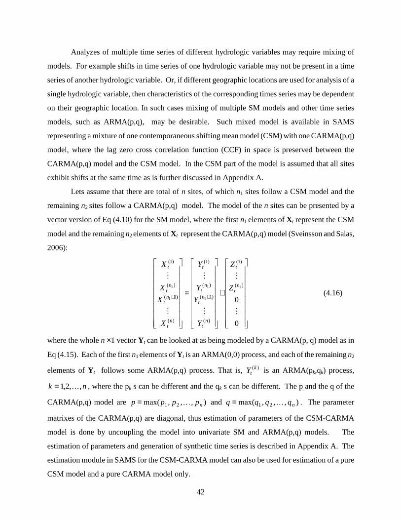
Lets assume that there are total of n sites, of which n1 sites follow a CSM model and the
remaining n2 sites follow a CARMA(p,q) model. The model of the n sites can be presented by a
vector version of Eq (4.10) for the SM model, where the first n1 elements of X t represent the CSM
model and the remaining n2 elements of X t represent the CARMA(p,q) model (Sveinsson and Salas,
2006):
+
=
++
0
0
)(
)1(
)(
)1(
)(
)1(
)(
)1(
)(
)1(
1
1
1
1
1
M
M
M
M
M
M
nt
t
nt
nt
nt
t
nt
nt
nt
t
Z
Z
Y
Y
Y
Y
X
X
X
X
(4.16)
where the whole n ×1 vector Y t can be looked at as being modeled by a CARMA(p, q) model as in
Eq (4.15). Each of the first n1 elements of Y t is an ARMA(0,0) process, and each of the remaining n2
elements of Y t follows some ARMA(p,q) process. That is, )(ktY is an ARMA(pk,qk) process,
nk ,,2,1 K= , where the pk s can be different and the qk s can be different. The p and the q of the
CARMA(p,q) model are ),,,max( 21 npppp K= and ),,,max( 21 nqqqq K= . The parameter
matrixes of the CARMA(p,q) are diagonal, thus estimation of parameters of the CSM-CARMA
model is done by uncoupling the model into univariate SM and ARMA(p,q) models. The
estimation of parameters and generation of synthetic time series is described in Appendix A. The
estimation module in SAMS for the CSM-CARMA model can also be used for estimation of a pure
CSM model and a pure CARMA model only.
43
The CSM-CARMA model is capable of preserving the lag zero cross correlation in space
between different sites, in addition to the time dependence structure for each site as defined by the
parameters p and q. In addition, the CSM portion of the model is capable of preserving a certain
dependence structure both in time and space through the noise level process Zt.
4.3.4 Multivariate Seasonal MPAR (p)
The MPAR(p) model for n sites can be expressed as:
τντνττν ,1
,,, εYY ∑=
− +Φ=p
iii (4.17)
Where τν ,Y is a n ×1 column vector of normally distributed zero mean elements representing the
process for year ν and season τ. The τττ ,,2,1 ,,, pΦΦΦ K are the n × n autoregressive periodic
parameter matrixes, and ( )ττν G0ε ,MVN~}{ , iid is the n ×1 vector of normally distributed noise
terms with mean zero and periodic n × n variance-covariance matrix Gτ. The noise vector is
independent in time and correlated in space at lag zero. For estimation of parameters and generation
of synthetic time series refer to Appendix A.
4.4 Disaggregation Models
Valencia and Schaake (1973) and later extension by Mejia and Rousselle (1976) introduced
the basic disaggregation model for temporal disaggregation of annual flows into seasonal flows.
However, the same model can also be used for spatial disaggregation. For example, the sum of flows
of several stations can be disaggregated into flows at each of these stations or the total flows at key
stations can be disaggregated into flows at substations which usually, but not necessarily, sum to
form the flows of the key stations. The Valencia and Schaake and the Mejia and Rousselle models
require many parameters to be estimated in the case of temporal disaggregation. For example,
Valencia and Schaake model requires 156 parameters for the case of disaggregating annual flows
into 12 seasons for one station. Mejia and Rouselle model require 168 parameters. For 3 sites, the
above models require 1,404 and 1,512 for both models, respectively. Lane (1979) introduced the
condensed model for temporal disaggregation which reduces the number of parameters required
drastically. For example, for the cases mentioned above, Lane's model requires 36 parameters for the
one site case and 324 parameters for the 3 site case. Later Grygier and Stedinger (1990) introduced a
contemporaneous temporal disaggregation model which requires 48 parameters for the above one
44
site case and 216 parameters for the above 3 site case.
In SAMS, Lane’s model and Grygier and Stedinger model are used for temporal (seasonal)
disaggregation, and the Valencia and Schaake model and Mejia and Rousselle model are used for
spatial disaggregation of annual and seasonal data.
In using disaggregation models for data generation, adjustments may be needed to ensure
additivity constraints. For instance, in spatial disaggregation, to ensure that the generated flows at
substations (or at subsequent stations) add to the total or a fraction (depending on the particular case
at hand) of the corresponding generated flow at a key station (or subkey station) or, in temporal
disaggregation, to ensure that the generated seasonal values add exactly to the generated annual
value, three methods of adjustment based on Lane and Frevert (1990) are provided in SAMS. These
methods will be described in the following sections.
4.4.1 Spatial Disaggregation of Annual Data
For spatial disaggregation of annual data from N key stations to M sub stations there are two
models available, namely the Valencia and Schaake (VS) model (Valencia and Schaake, 1973)
ννν εBXAY += (4.18)
and the Mejia and Rousselle (MR) model (Mejia and Rousselle, 1976)
1−++= νννν YCεBXAY (4.19)
where νX is the N × 1 column vector of observations in year ν at the N key sites, νY is the
corresponding M × 1 column vector at the sub sites, νε is the M × 1 column noise vector
uncorrelated in space and time with each element distributed as standard normal, and A, B, and C are
full M × N, M × M, and M × M parameter matrixes, respectively. The differences between the VS
and MR models is that the VS model is designed to preserve the lag 0 correlation coefficient in space
between all sub stations through the matrix B, and the lag 0 correlation in space between all sub and
key stations through the matrix A. The MR model additionally preserves the lag 1 correlation
coefficient in space between all sub stations through the matrix C, i.e. the correlations between
current year values with past year values. For estimation of parameters refer to Appendix A.
4.4.2 Spatial Disaggregation of Seasonal Data
For spatial disaggregation of seasonal data from N key stations to M sub stations only the MR
model is made available in SAMS although the simpler VS model could also be used. The reason
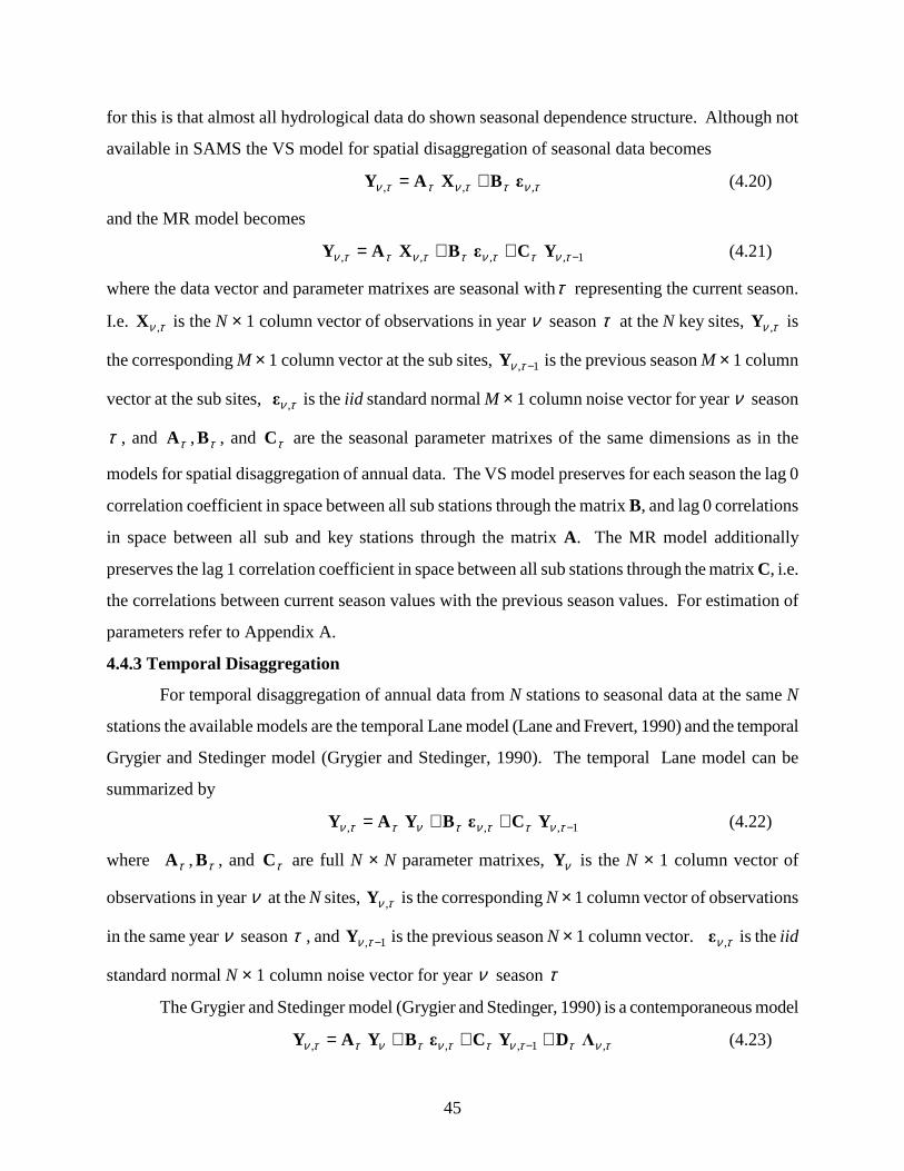
45
for this is that almost all hydrological data do shown seasonal dependence structure. Although not
available in SAMS the VS model for spatial disaggregation of seasonal data becomes
τνττνττν ,,, εBXAY += (4.20)
and the MR model becomes
1,,,, −++= τνττνττνττν YCεBXAY (4.21)
where the data vector and parameter matrixes are seasonal withτ representing the current season.
I.e. τν ,X is the N × 1 column vector of observations in year ν season τ at the N key sites, τν ,Y is
the corresponding M × 1 column vector at the sub sites, 1, −τνY is the previous season M × 1 column
vector at the sub sites, τν ,ε is the iid standard normal M × 1 column noise vector for year ν season
τ , and τA , τB , and τC are the seasonal parameter matrixes of the same dimensions as in the
models for spatial disaggregation of annual data. The VS model preserves for each season the lag 0
correlation coefficient in space between all sub stations through the matrix B, and lag 0 correlations
in space between all sub and key stations through the matrix A. The MR model additionally
preserves the lag 1 correlation coefficient in space between all sub stations through the matrix C, i.e.
the correlations between current season values with the previous season values. For estimation of
parameters refer to Appendix A.
4.4.3 Temporal Disaggregation
For temporal disaggregation of annual data from N stations to seasonal data at the same N
stations the available models are the temporal Lane model (Lane and Frevert, 1990) and the temporal
Grygier and Stedinger model (Grygier and Stedinger, 1990). The temporal Lane model can be
summarized by
1,,, −++= τνττντνττν YCεBYAY (4.22)
where τA , τB , and τC are full N × N parameter matrixes, νY is the N × 1 column vector of
observations in year ν at the N sites, τν ,Y is the corresponding N × 1 column vector of observations
in the same year ν season τ , and 1, −τνY is the previous season N × 1 column vector. τν ,ε is the iid
standard normal N × 1 column noise vector for year ν season τ
The Grygier and Stedinger model (Grygier and Stedinger, 1990) is a contemporaneous model
τνττνττντνττν ,1,,, ΛDYCεBYAY +++= − (4.23)
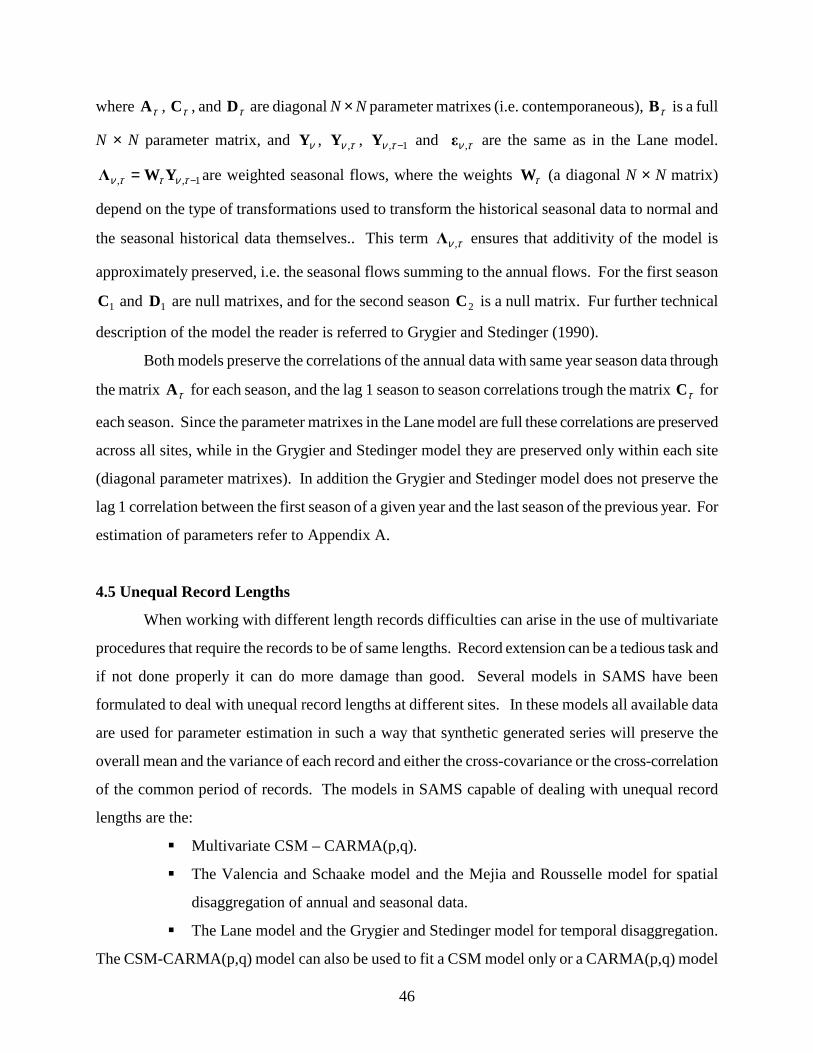
46
where τA , τC , and τD are diagonal N × N parameter matrixes (i.e. contemporaneous), τB is a full
N × N parameter matrix, and νY , τν ,Y , 1, −τνY and τν ,ε are the same as in the Lane model.
1,, −= τνττν YWΛ are weighted seasonal flows, where the weights τW (a diagonal N × N matrix)
depend on the type of transformations used to transform the historical seasonal data to normal and
the seasonal historical data themselves.. This term τν ,Λ ensures that additivity of the model is
approximately preserved, i.e. the seasonal flows summing to the annual flows. For the first season
1C and 1D are null matrixes, and for the second season 2C is a null matrix. Fur further technical
description of the model the reader is referred to Grygier and Stedinger (1990).
Both models preserve the correlations of the annual data with same year season data through
the matrix τA for each season, and the lag 1 season to season correlations trough the matrix τC for
each season. Since the parameter matrixes in the Lane model are full these correlations are preserved
across all sites, while in the Grygier and Stedinger model they are preserved only within each site
(diagonal parameter matrixes). In addition the Grygier and Stedinger model does not preserve the
lag 1 correlation between the first season of a given year and the last season of the previous year. For
estimation of parameters refer to Appendix A.
4.5 Unequal Record Lengths
When working with different length records difficulties can arise in the use of multivariate
procedures that require the records to be of same lengths. Record extension can be a tedious task and
if not done properly it can do more damage than good. Several models in SAMS have been
formulated to deal with unequal record lengths at different sites. In these models all available data
are used for parameter estimation in such a way that synthetic generated series will preserve the
overall mean and the variance of each record and either the cross-covariance or the cross-correlation
of the common period of records. The models in SAMS capable of dealing with unequal record
lengths are the:
� Multivariate CSM – CARMA(p,q).
� The Valencia and Schaake model and the Mejia and Rousselle model for spatial
disaggregation of annual and seasonal data.
� The Lane model and the Grygier and Stedinger model for temporal disaggregation.
The CSM-CARMA(p,q) model can also be used to fit a CSM model only or a CARMA(p,q) model
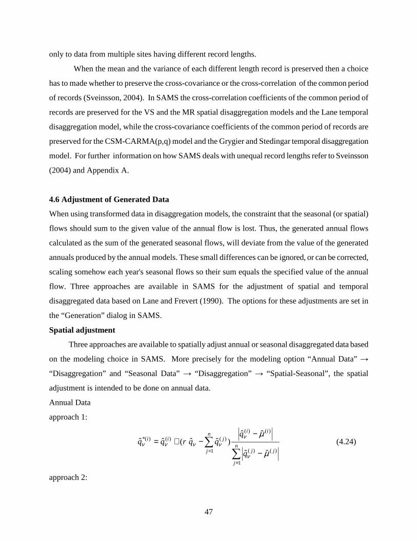
47
only to data from multiple sites having different record lengths.
When the mean and the variance of each different length record is preserved then a choice
has to made whether to preserve the cross-covariance or the cross-correlation of the common period
of records (Sveinsson, 2004). In SAMS the cross-correlation coefficients of the common period of
records are preserved for the VS and the MR spatial disaggregation models and the Lane temporal
disaggregation model, while the cross-covariance coefficients of the common period of records are
preserved for the CSM-CARMA(p,q) model and the Grygier and Stedingar temporal disaggregation
model. For further information on how SAMS deals with unequal record lengths refer to Sveinsson
(2004) and Appendix A.
4.6 Adjustment of Generated Data
When using transformed data in disaggregation models, the constraint that the seasonal (or spatial)
flows should sum to the given value of the annual flow is lost. Thus, the generated annual flows
calculated as the sum of the generated seasonal flows, will deviate from the value of the generated
annuals produced by the annual models. These small differences can be ignored, or can be corrected,
scaling somehow each year's seasonal flows so their sum equals the specified value of the annual
flow. Three approaches are available in SAMS for the adjustment of spatial and temporal
disaggregated data based on Lane and Frevert (1990). The options for these adjustments are set in
the “Generation” dialog in SAMS.
Spatial adjustment
Three approaches are available to spatially adjust annual or seasonal disaggregated data based
on the modeling choice in SAMS. More precisely for the modeling option “Annual Data” →
“Disaggregation” and “Seasonal Data” → “Disaggregation” → “Spatial-Seasonal”, the spatial
adjustment is intended to be done on annual data.
Annual Data
approach 1:
∑∑
=
= −
−−+=
n
j
jj
iin
j
jii
q
qqqrqq
1
)()(
)()(
1
)()()(*
ˆˆ
ˆˆ)ˆˆ(ˆˆ
µ
µ
ν
ννννν (4.24)
approach 2:
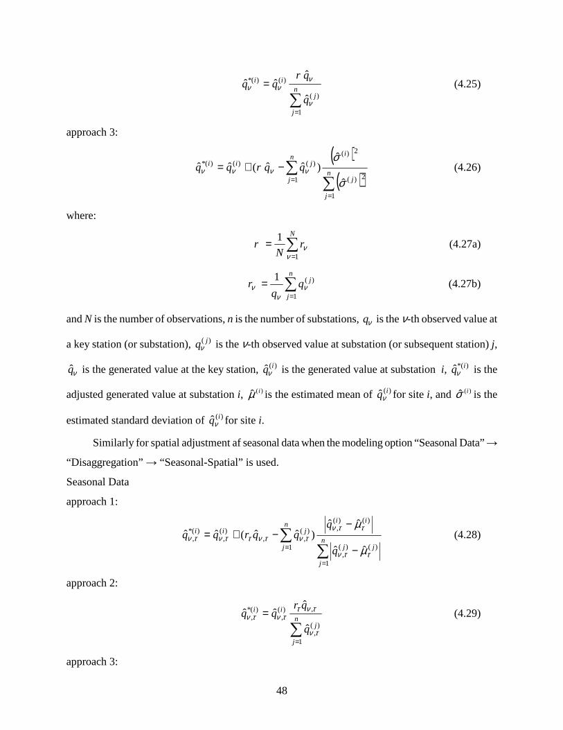
48
∑=
=n
j
j
ii
q
qrqq
1
)(
)()(*
ˆ
ˆˆˆ
ν
ννν (4.25)
approach 3:
( )
( )∑∑
=
=−+=
n
j
j
in
j
jii qqrqq
1
2)(
2)(
1
)()()(*
ˆ
ˆ)ˆˆ(ˆˆ
σ
σνννν (4.26)
where:
∑=
=N
rN
r1
1
νν (4.27a)
∑=
=n
j
jqq
r1
)(1ν
νν (4.27b)
and N is the number of observations, n is the number of substations, νq is the ν-th observed value at
a key station (or substation), )( jqν is the ν-th observed value at substation (or subsequent station) j,
νq is the generated value at the key station, )(ˆ iqν is the generated value at substation i, )*(ˆ iqν is the
adjusted generated value at substation i, )(ˆ iµ is the estimated mean of )(ˆ iqν for site i, and )(ˆ iσ is the
estimated standard deviation of )(ˆ iqν for site i.
Similarly for spatial adjustment af seasonal data when the modeling option “Seasonal Data” →
“Disaggregation” → “Seasonal-Spatial” is used.
Seasonal Data
approach 1:
∑∑
=
= −
−−+=
n
j
jj
iin
j
jii
q
qqqrqq
1
)()(,
)()(,
1
)(,,
)(,
)(*,
ˆˆ
ˆˆ)ˆˆ(ˆˆ
ττν
ττντντνττντν
µ
µ (4.28)
approach 2:
∑=
=n
j
j
ii
q
qrqq
1
)(,
,)(,
)(*,
ˆ
ˆˆˆ
τν
τνττντν (4.29)
approach 3:
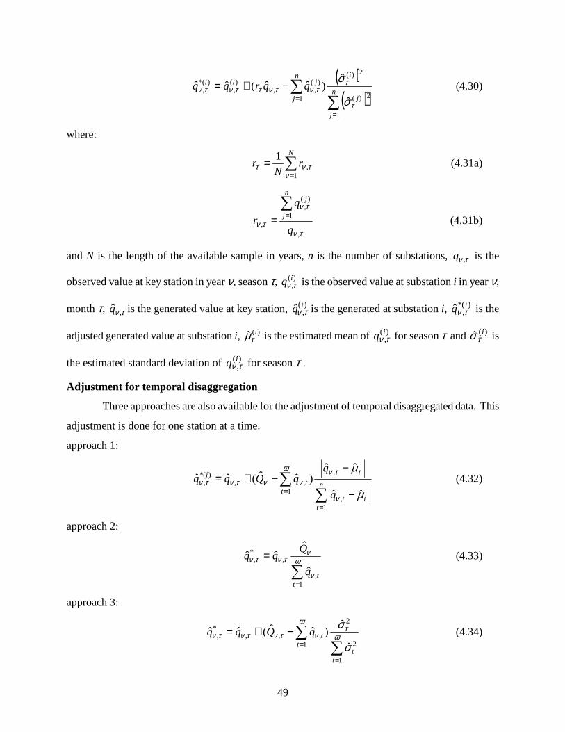
49
( )
( )∑∑
=
=−+=
n
j
j
in
j
jii qqrqq
1
2)(
2)(
1
)(,,
)(,
)(*,
ˆ
ˆ)ˆˆ(ˆˆ
τ
ττντνττντν
σ
σ (4.30)
where:
∑=
=N
rN
r1
,1
ντντ (4.31a)
τν
τν
τν,
1
)(,
,q
q
r
n
j
j∑== (4.31b)
and N is the length of the available sample in years, n is the number of substations, τν ,q is the
observed value at key station in year ν, season τ, )(,iq τν is the observed value at substation i in year ν,
month τ, τν ,q is the generated value at key station, )(,ˆ iq τν is the generated at substation i, )*(
,ˆ iq τν is the
adjusted generated value at substation i, )(ˆ iτµ is the estimated mean of )(
,iq τν for season τ and )(ˆ i
τσ is
the estimated standard deviation of )(,iq τν for season τ .
Adjustment for temporal disaggregation
Three approaches are also available for the adjustment of temporal disaggregated data. This
adjustment is done for one station at a time.
approach 1:
∑∑
=
= −
−−+=
n
ttt
tt
i
q
qqQqq
1,
,
1,,
)(*,
ˆˆ
ˆˆ)ˆˆ(ˆˆ
µ
µ
ν
ττνω
νντντν (4.32)
approach 2:
∑=
= ω
ν
ντντν
1,
,*,
ˆ
ˆˆˆ
ttq
Qqq (4.33)
approach 3:
∑∑
=
=−+= ω
τω
ντντντν
σ
σ
1
2
2
1,,,
*,
ˆ
ˆ)ˆˆ(ˆˆ
tt
ttqQqq (4.34)
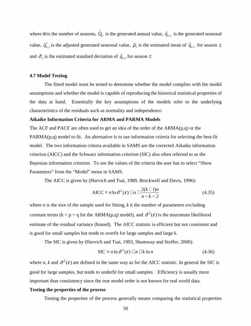
50
where ω is the number of seasons, νQ is the generated annual value, τν ,q is the generated seasonal
value, *,ˆ τνq is the adjusted generated seasonal value, τµ is the estimated mean of τν ,q for season τ,
and τσ is the estimated standard deviation of τν ,q for season τ.
4.7 Model Testing
The fitted model must be tested to determine whether the model complies with the model
assumptions and whether the model is capable of reproducing the historical statistical properties of
the data at hand. Essentially the key assumptions of the models refer to the underlying
characteristics of the residuals such as normality and independence.
Aikaike Information Criteria for ARMA and PARMA Mod els
The ACF and PACF are often used to get an idea of the order of the ARMA(p,q) or the
PARMA(p,q) model to fit. An alternative is to use information criteria for selecting the best-fit
model. The two information criteria available in SAMS are the corrected Aikaike information
criterion (AICC) and the Schwarz information criterion (SIC) also often referred to as the
Bayesian information criterion. To see the values of the criteria the user has to select “Show
Parameters” from the “Model” menu in SAMS.
The AICC is given by (Hurvich and Tsai, 1989, Brockwell and Davis, 1996):
2
)1(2)(ˆlnAICC 2
−−+++=kn
nknn εσ (4.35)
where n is the size of the sample used for fitting, k it the number of parameters excluding
constant terms (k = p + q for the ARMA(p,q) model), and )(ˆ 2 εσ is the maximum likelihood
estimate of the residual variance (biased). The AICC statistic is efficient but not consistent and
is good for small samples but tends to overfit for large samples and large k.
The SIC is given by (Hurvich and Tsai, 1993, Shumway and Stoffer, 2000):
nknn ln)(ˆlnSIC 2 ++= εσ (4.36)
where n, k and )(ˆ 2 εσ are defined in the same way as for the AICC statistic. In general the SIC is
good for large samples, but tends to underfit for small samples. Efficiency is usually more
important than consistency since the true model order is not known for real world data.
Testing the properties of the process
Testing the properties of the process generally means comparing the statistical properties
51
(statistics) of the process being modeled, for instance, the process τν ,Y , with those of the historical
sample. In general, one would like the model to be capable of reproducing the necessary statistics
that affect the variability of the data. Furthermore, the model should be capable of reproducing
certain statistics that are related to the intended use of the model.
If τν ,Y has been previously transformed from τν ,X , the original non-normal process, then one
must test, in addition to the statistical properties of Y, some of the properties of X. Generally, the
properties of Y include the seasonal mean, seasonal variance, seasonal skewness, and season-to-
season correlations and cross-correlations (in the case of multisite processes), and the properties of X
include the seasonal mean, variance, skewness, correlations, and cross-correlations (for multisite
systems). Furthermore, additional properties of τν ,X such as those related to low flows, high flows,
droughts, and storage may be included depending on the particular problem at hand.
In addition, it is often the case that not only the properties of the seasonal processes τν ,Y and
τν ,X , must be tested but also the properties of the corresponding annual processes AY and AX . For
example, this case arises when designing the storage capacity of reservoir systems or when testing
the performance of reservoir systems of given capacities, in which one or more reservoirs are for
over year regulation. In such cases the annual properties considered are usually the mean, variance,
skewness, autocorrelations, cross-correlations (for multisite systems), and more complex properties
such as those related to droughts and storage.
The comparison of the statistical properties of the process being modeled versus the historical
properties may be done in two ways. Depending on the type of model, certain properties of the Y
process such as the mean(s), variance(s), and covariance(s), can be derived from the model in close
form. If the method of moments is used for parameter estimation, the mean(s), variance(s), and some
of the covariance should be reproduced exactly, however, except for the mean, that may not be the
case for other estimation methods. Finding properties of the Y process in closed form beyond the
first two moments, for instance, drought related properties, are complex and generally are not
available for most models. Likewise, except for simple models, finding properties in close form for
the corresponding annual process AY, is not simple either. In such cases, the required statistical
properties are derived by data generation.
Data generation studies for comparing statistical properties of the underlying process Y (and
other derived processes such as AY, X and AX) are generally undertaken based on samples of equal
52
length as the length of the historical record and based on a certain number of samples which can give
enough precision for estimating the statistical properties of concern. While there are some statistical
rules that can be derived to determine the number of samples required, a practical rule is to generate
say 100 samples which can give an idea of the distribution of the statistic of interest say θ. In any
case, the statistics θ(i), i = 1, ...,100 are estimated from the 100 samples and the mean θ and
variance s2(θ) are determined. Then, the mean deviation, MD(θ)
)()( HMD θθθ −= (4.37)
and the relative root mean square deviations, RRMSD(θ)
∑ =−= 100
12])([
)(
1)(
i i HH
RRMSD θθθ
θ (4.38)
are obtained in which θ(H)is the statistic derived from the historical sample (historical statistic). The
statistics MD(θ) and RRMSD(θ) are useful for comparing between the historical and model statistics
derived by data generation. In addition, one can observe where θ(H) falls relative to θ - s(θ) and θ
+ s(θ). Also graphical comparisons such as the Box-Cox diagrams can be useful.
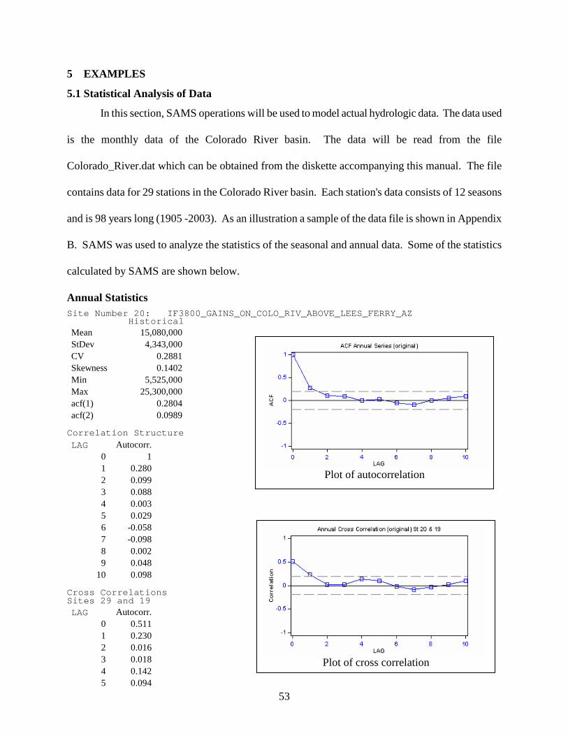
53
5 EXAMPLES
5.1 Statistical Analysis of Data
In this section, SAMS operations will be used to model actual hydrologic data. The data used
is the monthly data of the Colorado River basin. The data will be read from the file
Colorado_River.dat which can be obtained from the diskette accompanying this manual. The file
contains data for 29 stations in the Colorado River basin. Each station's data consists of 12 seasons
and is 98 years long (1905 -2003). As an illustration a sample of the data file is shown in Appendix
B. SAMS was used to analyze the statistics of the seasonal and annual data. Some of the statistics
calculated by SAMS are shown below.
Annual Statistics Site Number 20: IF3800_GAINS_ON_COLO_RIV_ABOVE_LEES_FERRY_AZ Historical Mean 15,080,000 StDev 4,343,000 CV 0.2881 Skewness 0.1402 Min 5,525,000 Max 25,300,000 acf(1) 0.2804 acf(2) 0.0989 Correlation Structure
LAG Autocorr. 0 1 1 0.280 2 0.099 3 0.088 4 0.003 5 0.029 6 -0.058 7 -0.098 8 0.002 9 0.048
10 0.098 Cross Correlations Sites 29 and 19 LAG Autocorr.
0 0.511 1 0.230 2 0.016 3 0.018 4 0.142 5 0.094
Plot of autocorrelation
Plot of cross correlation
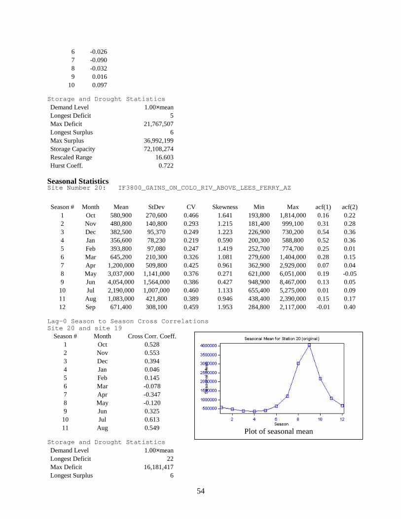
54
6 -0.026 7 -0.090 8 -0.032 9 0.016
10 0.097 Storage and Drought Statistics Demand Level 1.00×mean Longest Deficit 5 Max Deficit 21,767,507 Longest Surplus 6 Max Surplus 36,992,199 Storage Capacity 72,108,274 Rescaled Range 16.603 Hurst Coeff. 0.722
Seasonal Statistics Site Number 20: IF3800_GAINS_ON_COLO_RIV_ABOVE_LEES_FERRY_AZ Season # Month Mean StDev CV Skewness Min Max acf(1) acf(2)
1 Oct 580,900 270,600 0.466 1.641 193,800 1,814,000 0.16 0.22 2 Nov 480,800 140,800 0.293 1.215 181,400 999,100 0.31 0.28 3 Dec 382,500 95,370 0.249 1.223 226,900 730,200 0.54 0.36 4 Jan 356,600 78,230 0.219 0.590 200,300 588,800 0.52 0.36 5 Feb 393,800 97,080 0.247 1.419 252,700 774,700 0.25 0.01 6 Mar 645,200 210,300 0.326 1.081 279,600 1,404,000 0.28 0.15 7 Apr 1,200,000 509,800 0.425 0.961 362,900 2,929,000 0.07 0.04 8 May 3,037,000 1,141,000 0.376 0.271 621,000 6,051,000 0.19 -0.05 9 Jun 4,054,000 1,564,000 0.386 0.427 948,900 8,467,000 0.13 0.05 10 Jul 2,190,000 1,007,000 0.460 1.133 655,400 5,275,000 0.01 0.09 11 Aug 1,083,000 421,800 0.389 0.946 438,400 2,390,000 0.15 0.17 12 Sep 671,400 308,100 0.459 1.953 284,800 2,117,000 -0.01 0.40
Lag-0 Season to Season Cross Correlations Site 20 and site 19
Season # Month Cross Corr. Coeff. 1 Oct 0.528 2 Nov 0.553 3 Dec 0.394 4 Jan 0.046 5 Feb 0.145 6 Mar -0.078 7 Apr -0.347 8 May -0.120 9 Jun 0.325 10 Jul 0.613 11 Aug 0.549
Storage and Drought Statistics Demand Level 1.00×mean Longest Deficit 22 Max Deficit 16,181,417 Longest Surplus 6
Plot of seasonal mean

55
Max Surplus 13,728,208 Storage Capacity 77,644,242 Rescaled Range 58.069 Hurst Coeff. 0.637
5.2 Stochastic Modeling and Generation of Streamflow Data
SAMS was used to model the annual and monthly flows of site 20 of Colorado River basin
(refer to file Colorado_River.dat). Both annual and monthly data used in the following examples are
transformed using logarithmic transformation and the transformation coefficients are shown in
Appendix D.
5.2.1 Univariate ARMA(p,q) Model
SAMS was used to model the annual flows of site 20 with an ARMA(1,1) model. The MOM
was used to estimate the model parameters. SAMS was also used to generate 100 samples each 98
years long using the estimated parameters. The following is a summary of the results of the model
fitting and generation by using the ARMA(1,1) model.
Results of fitting an ARMA(1,1) model to the transformed and standardized annual flows of
site 20:
Model: ARMA
Model Parameters
Current_Model: ARMA(1,1) For Site(s): 20 Model Fitted To: Mean Subtracted Data MEAN_AND_VARIANCE: Mean: 15,076,300 Variance: 1.886×10¹³ AICC: 3091.860 SIC: 3094.775 PARAMETERS: White_Noise_Variance: 1.737×10¹³ AR_PARAMETERS: PHI(1): 0.352827 MA_PARAMETERS: THT(1): 0.078648
Results of statistical analysis of the data generated from the ARMA(1,1) model: Site Number 20: IF3800_GAINS_ON_COLO_RIV_ABOVE_LEES_FERRY_AZ
Statistics Historical Generated
Mean
15,080,000 15090000 StDev 4,343,000 4264000
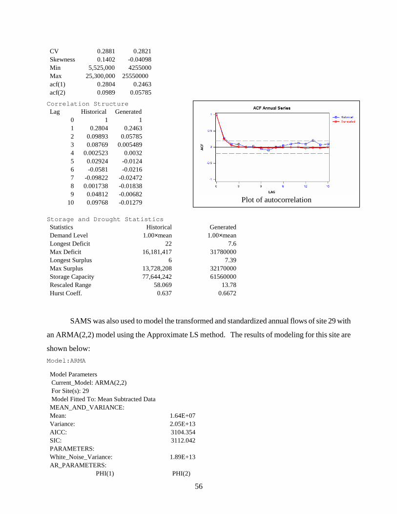
56
CV 0.2881 0.2821 Skewness 0.1402 -0.04098 Min 5,525,000 4255000 Max 25,300,000 25550000 acf(1) 0.2804 0.2463 acf(2) 0.0989 0.05785 Correlation Structure Lag Historical Generated
0 1 1 1 0.2804 0.2463 2 0.09893 0.05785 3 0.08769 0.005489 4 0.002523 0.0032 5 0.02924 -0.0124 6 -0.0581 -0.0216 7 -0.09822 -0.02472 8 0.001738 -0.01838 9 0.04812 -0.00682
10 0.09768 -0.01279 Storage and Drought Statistics Statistics Historical Generated Demand Level 1.00×mean 1.00×mean Longest Deficit 22 7.6 Max Deficit 16,181,417 31780000 Longest Surplus 6 7.39 Max Surplus 13,728,208 32170000 Storage Capacity 77,644,242 61560000 Rescaled Range 58.069 13.78 Hurst Coeff. 0.637 0.6672
SAMS was also used to model the transformed and standardized annual flows of site 29 with
an ARMA(2,2) model using the Approximate LS method. The results of modeling for this site are
shown below:
Model:ARMA Model Parameters Current_Model: ARMA(2,2) For Site(s): 29 Model Fitted To: Mean Subtracted Data MEAN_AND_VARIANCE: Mean: 1.64E+07 Variance: 2.05E+13 AICC: 3104.354 SIC: 3112.042 PARAMETERS: White_Noise_Variance: 1.89E+13 AR_PARAMETERS:
PHI(1) PHI(2)
Plot of autocorrelation
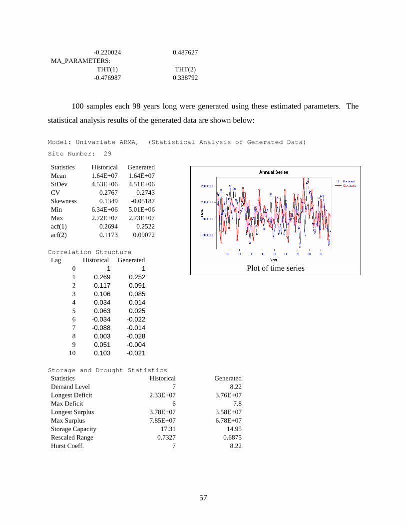
57
-0.220024 0.487627 MA_PARAMETERS:
THT(1) THT(2) -0.476987 0.338792
100 samples each 98 years long were generated using these estimated parameters. The
statistical analysis results of the generated data are shown below:
Model: Univariate ARMA, (Statistical Analysis of Generated Data) Site Number: 29 Statistics Historical Generated Mean 1.64E+07 1.64E+07 StDev 4.53E+06 4.51E+06 CV 0.2767 0.2743 Skewness 0.1349 -0.05187 Min 6.34E+06 5.01E+06 Max 2.72E+07 2.73E+07 acf(1) 0.2694 0.2522 acf(2) 0.1173 0.09072 Correlation Structure Lag Historical Generated
0 1 1 1 0.269 0.252 2 0.117 0.091 3 0.106 0.085 4 0.034 0.014 5 0.063 0.025 6 -0.034 -0.022 7 -0.088 -0.014 8 0.003 -0.028 9 0.051 -0.004
10 0.103 -0.021 Storage and Drought Statistics Statistics Historical Generated Demand Level 7 8.22 Longest Deficit 2.33E+07 3.76E+07 Max Deficit 6 7.8 Longest Surplus 3.78E+07 3.58E+07 Max Surplus 7.85E+07 6.78E+07 Storage Capacity 17.31 14.95 Rescaled Range 0.7327 0.6875 Hurst Coeff. 7 8.22
Plot of time series
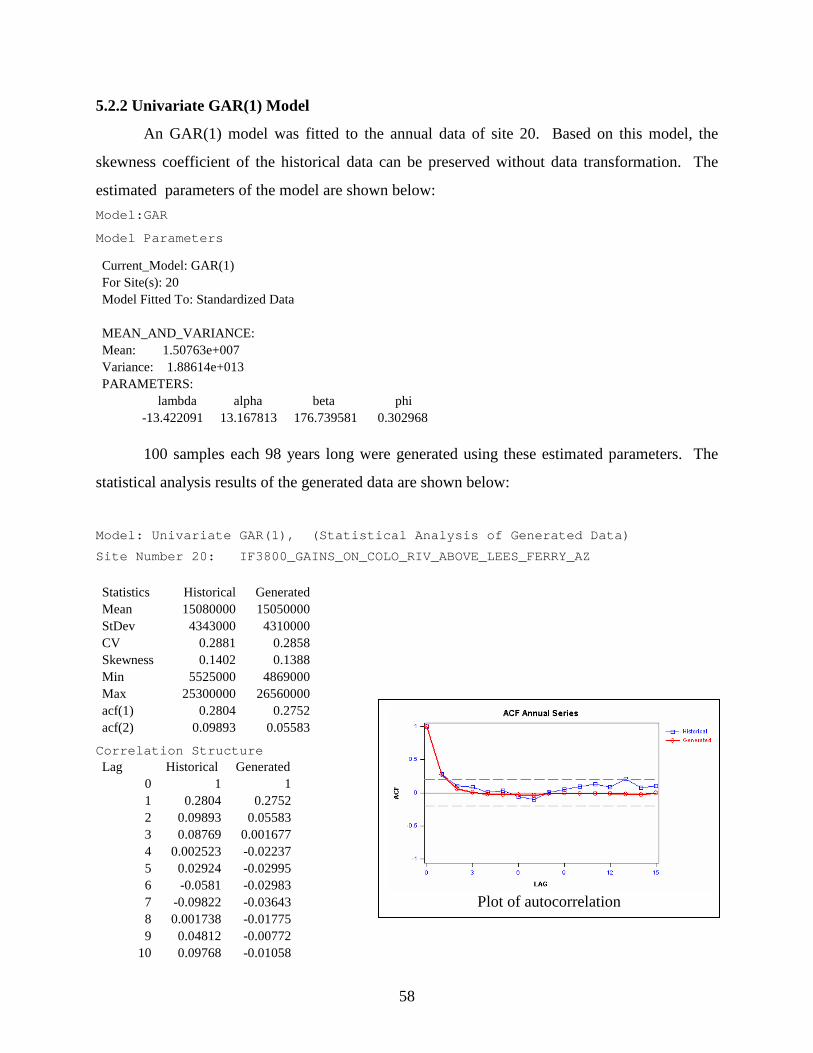
58
5.2.2 Univariate GAR(1) Model
An GAR(1) model was fitted to the annual data of site 20. Based on this model, the
skewness coefficient of the historical data can be preserved without data transformation. The
estimated parameters of the model are shown below:
Model:GAR Model Parameters
Current_Model: GAR(1) For Site(s): 20 Model Fitted To: Standardized Data MEAN_AND_VARIANCE: Mean: 1.50763e+007 Variance: 1.88614e+013 PARAMETERS:
lambda alpha beta phi -13.422091 13.167813 176.739581 0.302968
100 samples each 98 years long were generated using these estimated parameters. The
statistical analysis results of the generated data are shown below:
Model: Univariate GAR(1), (Statistical Analysis of Generated Data)
Site Number 20: IF3800_GAINS_ON_COLO_RIV_ABOVE_LEES_FERRY_AZ
Statistics Historical Generated Mean 15080000 15050000 StDev 4343000 4310000 CV 0.2881 0.2858 Skewness 0.1402 0.1388 Min 5525000 4869000 Max 25300000 26560000 acf(1) 0.2804 0.2752 acf(2) 0.09893 0.05583 Correlation Structure Lag Historical Generated
0 1 1 1 0.2804 0.2752 2 0.09893 0.05583 3 0.08769 0.001677 4 0.002523 -0.02237 5 0.02924 -0.02995 6 -0.0581 -0.02983 7 -0.09822 -0.03643 8 0.001738 -0.01775 9 0.04812 -0.00772
10 0.09768 -0.01058
Plot of autocorrelation
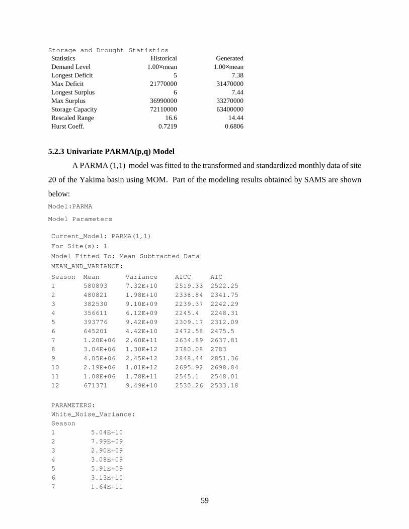
59
Storage and Drought Statistics Statistics Historical Generated Demand Level 1.00×mean 1.00×mean Longest Deficit 5 7.38 Max Deficit 21770000 31470000 Longest Surplus 6 7.44 Max Surplus 36990000 33270000 Storage Capacity 72110000 63400000 Rescaled Range 16.6 14.44 Hurst Coeff. 0.7219 0.6806
5.2.3 Univariate PARMA(p,q) Model
A PARMA (1,1) model was fitted to the transformed and standardized monthly data of site
20 of the Yakima basin using MOM. Part of the modeling results obtained by SAMS are shown
below:
Model:PARMA Model Parameters
Current_Model: PARMA(1,1)
For Site(s): 1
Model Fitted To: Mean Subtracted Data
MEAN_AND_VARIANCE:
Season Mean Variance AICC AIC
1 580893 7.32E+10 2519.33 2522.25
2 480821 1.98E+10 2338.84 2341.75
3 382530 9.10E+09 2239.37 2242.29
4 356611 6.12E+09 2245.4 2248.31
5 393776 9.42E+09 2309.17 2312.09
6 645201 4.42E+10 2472.58 2475.5
7 1.20E+06 2.60E+11 2634.89 2637.81
8 3.04E+06 1.30E+12 2780.08 2783
9 4.05E+06 2.45E+12 2848.44 2851.36
10 2.19E+06 1.01E+12 2695.92 2698.84
11 1.08E+06 1.78E+11 2545.1 2548.01
12 671371 9.49E+10 2530.26 2533.18
PARAMETERS:
White_Noise_Variance:
Season
1 5.04E+10
2 7.99E+09
3 2.90E+09
4 3.08E+09
5 5.91E+09
6 3.13E+10
7 1.64E+11
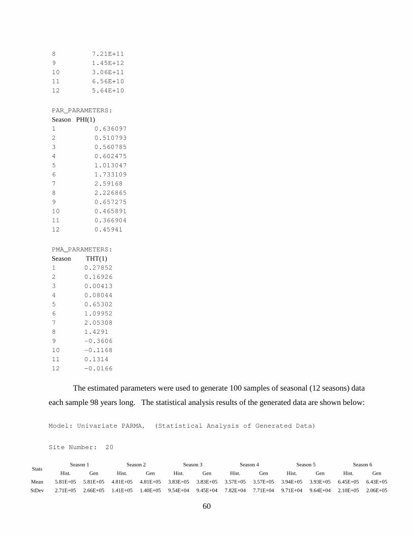
60
8 7.21E+11
9 1.45E+12
10 3.06E+11
11 6.56E+10
12 5.64E+10
PAR_PARAMETERS:
Season PHI(1) 1 0.636097
2 0.510793
3 0.560785
4 0.602475
5 1.013047
6 1.733109
7 2.59168
8 2.226865
9 0.657275
10 0.465891
11 0.366904
12 0.45941
PMA_PARAMETERS:
Season THT(1) 1 0.27852
2 0.16926
3 0.00413
4 0.08044
5 0.65302
6 1.09952
7 2.05308
8 1.4291
9 -0.3606
10 -0.1168
11 0.1314
12 -0.0166
The estimated parameters were used to generate 100 samples of seasonal (12 seasons) data
each sample 98 years long. The statistical analysis results of the generated data are shown below:
Model: Univariate PARMA, (Statistical Analysis of Generated Data)
Site Number: 20
Season 1 Season 2 Season 3 Season 4 Season 5 Season 6
Stats Hist. Gen Hist. Gen Hist. Gen Hist. Gen Hist. Gen Hist. Gen
Mean 5.81E+05 5.81E+05 4.81E+05 4.81E+05 3.83E+05 3.83E+05 3.57E+05 3.57E+05 3.94E+05 3.93E+05 6.45E+05 6.43E+05
StDev 2.71E+05 2.66E+05 1.41E+05 1.40E+05 9.54E+04 9.45E+04 7.82E+04 7.71E+04 9.71E+04 9.64E+04 2.10E+05 2.06E+05
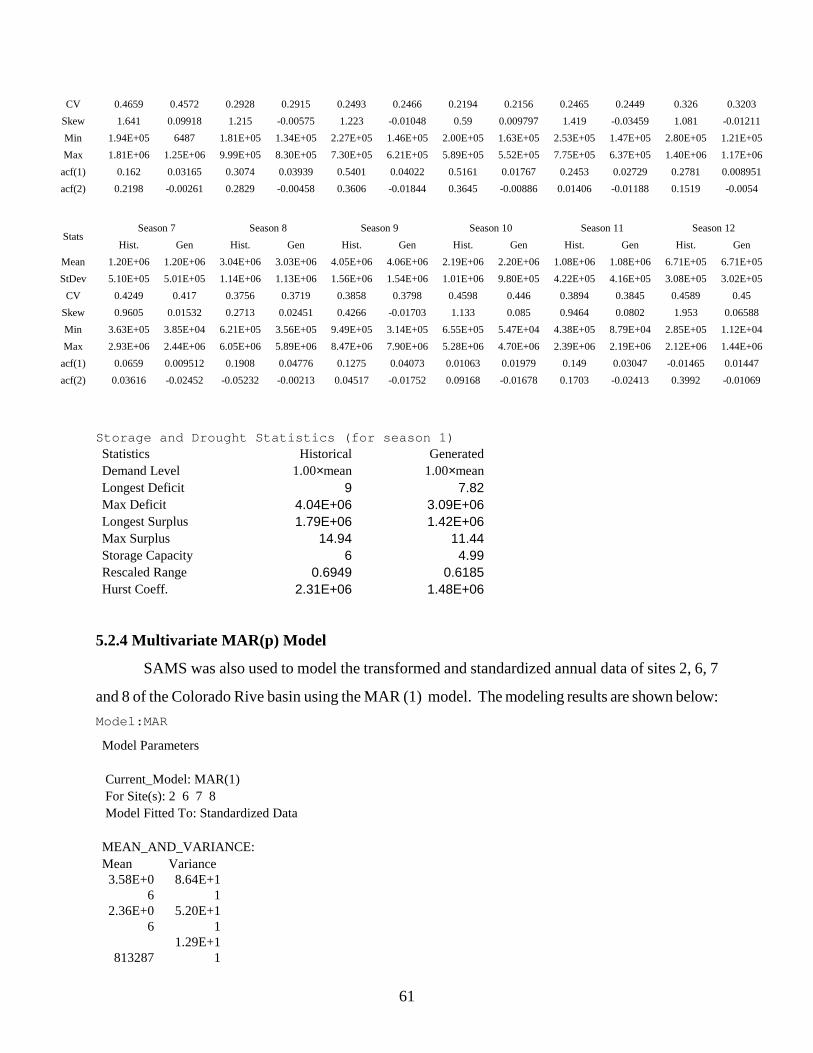
61
CV 0.4659 0.4572 0.2928 0.2915 0.2493 0.2466 0.2194 0.2156 0.2465 0.2449 0.326 0.3203
Skew 1.641 0.09918 1.215 -0.00575 1.223 -0.01048 0.59 0.009797 1.419 -0.03459 1.081 -0.01211
Min 1.94E+05 6487 1.81E+05 1.34E+05 2.27E+05 1.46E+05 2.00E+05 1.63E+05 2.53E+05 1.47E+05 2.80E+05 1.21E+05
Max 1.81E+06 1.25E+06 9.99E+05 8.30E+05 7.30E+05 6.21E+05 5.89E+05 5.52E+05 7.75E+05 6.37E+05 1.40E+06 1.17E+06
acf(1) 0.162 0.03165 0.3074 0.03939 0.5401 0.04022 0.5161 0.01767 0.2453 0.02729 0.2781 0.008951
acf(2) 0.2198 -0.00261 0.2829 -0.00458 0.3606 -0.01844 0.3645 -0.00886 0.01406 -0.01188 0.1519 -0.0054
Season 7 Season 8 Season 9 Season 10 Season 11 Season 12 Stats
Hist. Gen Hist. Gen Hist. Gen Hist. Gen Hist. Gen Hist. Gen
Mean 1.20E+06 1.20E+06 3.04E+06 3.03E+06 4.05E+06 4.06E+06 2.19E+06 2.20E+06 1.08E+06 1.08E+06 6.71E+05 6.71E+05
StDev 5.10E+05 5.01E+05 1.14E+06 1.13E+06 1.56E+06 1.54E+06 1.01E+06 9.80E+05 4.22E+05 4.16E+05 3.08E+05 3.02E+05
CV 0.4249 0.417 0.3756 0.3719 0.3858 0.3798 0.4598 0.446 0.3894 0.3845 0.4589 0.45
Skew 0.9605 0.01532 0.2713 0.02451 0.4266 -0.01703 1.133 0.085 0.9464 0.0802 1.953 0.06588
Min 3.63E+05 3.85E+04 6.21E+05 3.56E+05 9.49E+05 3.14E+05 6.55E+05 5.47E+04 4.38E+05 8.79E+04 2.85E+05 1.12E+04
Max 2.93E+06 2.44E+06 6.05E+06 5.89E+06 8.47E+06 7.90E+06 5.28E+06 4.70E+06 2.39E+06 2.19E+06 2.12E+06 1.44E+06
acf(1) 0.0659 0.009512 0.1908 0.04776 0.1275 0.04073 0.01063 0.01979 0.149 0.03047 -0.01465 0.01447
acf(2) 0.03616 -0.02452 -0.05232 -0.00213 0.04517 -0.01752 0.09168 -0.01678 0.1703 -0.02413 0.3992 -0.01069 Storage and Drought Statistics (for season 1) Statistics Historical Generated Demand Level 1.00×mean 1.00×mean Longest Deficit 9 7.82 Max Deficit 4.04E+06 3.09E+06 Longest Surplus 1.79E+06 1.42E+06 Max Surplus 14.94 11.44 Storage Capacity 6 4.99 Rescaled Range 0.6949 0.6185 Hurst Coeff. 2.31E+06 1.48E+06
5.2.4 Multivariate MAR(p) Model
SAMS was also used to model the transformed and standardized annual data of sites 2, 6, 7
and 8 of the Colorado Rive basin using the MAR (1) model. The modeling results are shown below:
Model:MAR
Model Parameters Current_Model: MAR(1) For Site(s): 2 6 7 8 Model Fitted To: Standardized Data MEAN_AND_VARIANCE: Mean Variance 3.58E+0
6 8.64E+1
1 2.36E+0
6 5.20E+1
1
813287 1.29E+1
1
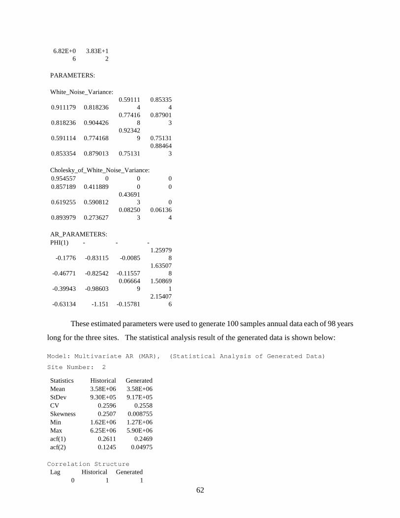
62
6.82E+06
3.83E+12
PARAMETERS: White_Noise_Variance:
0.911179 0.818236 0.59111
4 0.85335
4
0.818236 0.904426 0.77416
8 0.87901
3
0.591114 0.774168 0.92342
9 0.75131
0.853354 0.879013 0.75131 0.88464
3 Cholesky_of_White_Noise_Variance: 0.954557 0 0 0 0.857189 0.411889 0 0
0.619255 0.590812 0.43691
3 0
0.893979 0.273627 0.08250
3 0.06136
4 AR_PARAMETERS: PHI(1) - - -
-0.1776 -0.83115 -0.0085 1.25979
8
-0.46771 -0.82542 -0.11557 1.63507
8
-0.39943 -0.98603 0.06664
9 1.50869
1
-0.63134 -1.151 -0.15781 2.15407
6
These estimated parameters were used to generate 100 samples annual data each of 98 years
long for the three sites. The statistical analysis result of the generated data is shown below:
Model: Multivariate AR (MAR), (Statistical Analysis of Generated Data) Site Number: 2 Statistics Historical Generated Mean 3.58E+06 3.58E+06 StDev 9.30E+05 9.17E+05 CV 0.2596 0.2558 Skewness 0.2507 0.008755 Min 1.62E+06 1.27E+06 Max 6.25E+06 5.90E+06 acf(1) 0.2611 0.2469 acf(2) 0.1245 0.04975 Correlation Structure Lag Historical Generated
0 1 1
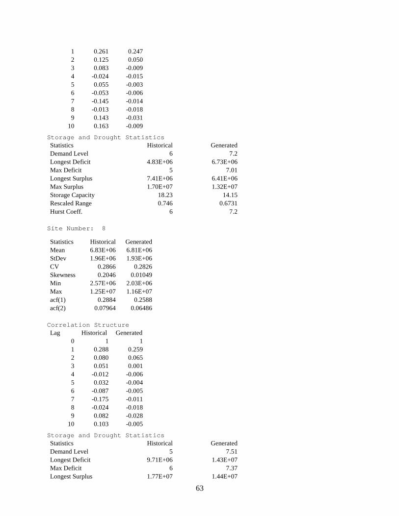
63
1 0.261 0.247 2 0.125 0.050 3 0.083 -0.009 4 -0.024 -0.015 5 0.055 -0.003 6 -0.053 -0.006 7 -0.145 -0.014 8 -0.013 -0.018 9 0.143 -0.031
10 0.163 -0.009 Storage and Drought Statistics Statistics Historical Generated Demand Level 6 7.2 Longest Deficit 4.83E+06 6.73E+06 Max Deficit 5 7.01 Longest Surplus 7.41E+06 6.41E+06 Max Surplus 1.70E+07 1.32E+07 Storage Capacity 18.23 14.15 Rescaled Range 0.746 0.6731 Hurst Coeff. 6 7.2 Site Number: 8 Statistics Historical Generated Mean 6.83E+06 6.81E+06 StDev 1.96E+06 1.93E+06 CV 0.2866 0.2826 Skewness 0.2046 0.01049 Min 2.57E+06 2.03E+06 Max 1.25E+07 1.16E+07 acf(1) 0.2884 0.2588 acf(2) 0.07964 0.06486 Correlation Structure Lag Historical Generated
0 1 1 1 0.288 0.259 2 0.080 0.065 3 0.051 0.001 4 -0.012 -0.006 5 0.032 -0.004 6 -0.087 -0.005 7 -0.175 -0.011 8 -0.024 -0.018 9 0.082 -0.028
10 0.103 -0.005 Storage and Drought Statistics Statistics Historical Generated Demand Level 5 7.51 Longest Deficit 9.71E+06 1.43E+07 Max Deficit 6 7.37 Longest Surplus 1.77E+07 1.44E+07
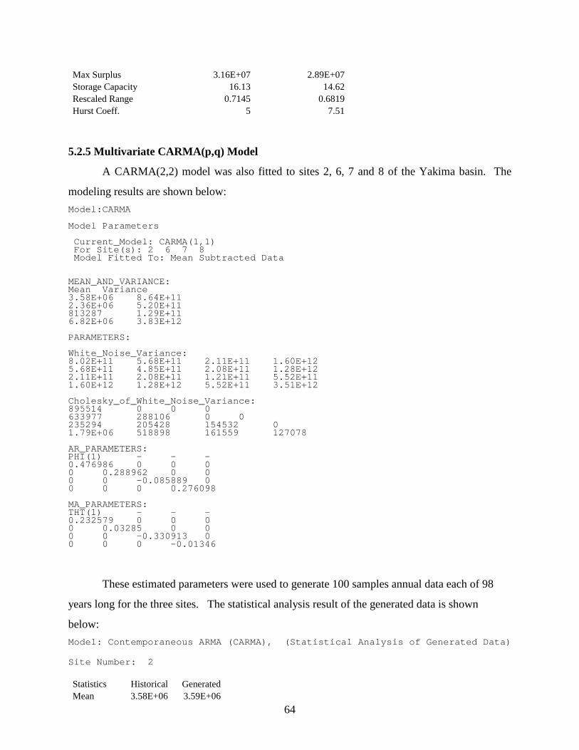
64
Max Surplus 3.16E+07 2.89E+07 Storage Capacity 16.13 14.62 Rescaled Range 0.7145 0.6819 Hurst Coeff. 5 7.51
5.2.5 Multivariate CARMA(p,q) Model
A CARMA(2,2) model was also fitted to sites 2, 6, 7 and 8 of the Yakima basin. The
modeling results are shown below:
Model:CARMA Model Parameters Current_Model: CARMA(1,1) For Site(s): 2 6 7 8 Model Fitted To: Mean Subtracted Data MEAN_AND_VARIANCE: Mean Variance 3.58E+06 8.64E+11 2.36E+06 5.20E+11 813287 1.29E+11 6.82E+06 3.83E+12 PARAMETERS: White_Noise_Variance: 8.02E+11 5.68E+11 2.11E+11 1.60E+12 5.68E+11 4.85E+11 2.08E+11 1.28E+12 2.11E+11 2.08E+11 1.21E+11 5.52E+11 1.60E+12 1.28E+12 5.52E+11 3.51E+12 Cholesky_of_White_Noise_Variance: 895514 0 0 0 633977 288106 0 0 235294 205428 154532 0 1.79E+06 518898 161559 127078 AR_PARAMETERS: PHI(1) - - - 0.476986 0 0 0 0 0.288962 0 0 0 0 -0.085889 0 0 0 0 0.276098 MA_PARAMETERS: THT(1) - - - 0.232579 0 0 0 0 0.03285 0 0 0 0 -0.330913 0 0 0 0 -0.01346
These estimated parameters were used to generate 100 samples annual data each of 98
years long for the three sites. The statistical analysis result of the generated data is shown
below:
Model: Contemporaneous ARMA (CARMA), (Statistical Analysis of Generated Data) Site Number: 2 Statistics Historical Generated Mean 3.58E+06 3.59E+06
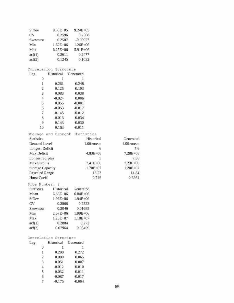
65
StDev 9.30E+05 9.24E+05 CV 0.2596 0.2568 Skewness 0.2507 -0.00927 Min 1.62E+06 1.26E+06 Max 6.25E+06 5.91E+06 acf(1) 0.2611 0.2477 acf(2) 0.1245 0.1032 Correlation Structure Lag Historical Generated
0 1 1 1 0.261 0.248 2 0.125 0.103 3 0.083 0.038 4 -0.024 0.006 5 0.055 -0.001 6 -0.053 -0.017 7 -0.145 -0.012 8 -0.013 -0.034 9 0.143 -0.030
10 0.163 -0.011 Storage and Drought Statistics Statistics Historical Generated Demand Level 1.00×mean 1.00×mean Longest Deficit 6 7.6 Max Deficit 4.83E+06 7.28E+06 Longest Surplus 5 7.56 Max Surplus 7.41E+06 7.23E+06 Storage Capacity 1.70E+07 1.28E+07 Rescaled Range 18.23 14.84 Hurst Coeff. 0.746 0.6864 Site Number: 8 Statistics Historical Generated Mean 6.83E+06 6.84E+06 StDev 1.96E+06 1.94E+06 CV 0.2866 0.2832 Skewness 0.2046 0.01695 Min 2.57E+06 1.99E+06 Max 1.25E+07 1.18E+07 acf(1) 0.2884 0.272 acf(2) 0.07964 0.06459 Correlation Structure Lag Historical Generated
0 1 1 1 0.288 0.272 2 0.080 0.065 3 0.051 0.007 4 -0.012 -0.010 5 0.032 -0.011 6 -0.087 -0.017 7 -0.175 -0.004
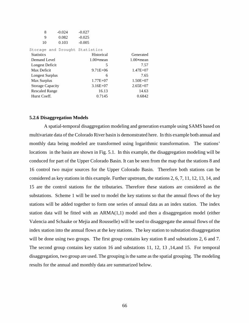
66
8 -0.024 -0.027 9 0.082 -0.025
10 0.103 -0.005 Storage and Drought Statistics Statistics Historical Generated Demand Level 1.00×mean 1.00×mean Longest Deficit 5 7.57 Max Deficit 9.71E+06 1.47E+07 Longest Surplus 6 7.65 Max Surplus 1.77E+07 1.50E+07 Storage Capacity 3.16E+07 2.65E+07 Rescaled Range 16.13 14.63 Hurst Coeff. 0.7145 0.6842
5.2.6 Disaggregation Models
A spatial-temporal disaggregation modeling and generation example using SAMS based on
multivariate data of the Colorado River basin is demonstrated here. In this example both annual and
monthly data being modeled are transformed using logarithmic transformation. The stations’
locations in the basin are shown in Fig. 5.1. In this example, the disaggregation modeling will be
conduced for part of the Upper Colorado Basin. It can be seen from the map that the stations 8 and
16 control two major sources for the Upper Colorado Basin. Therefore both stations can be
considered as key stations in this example. Further upstream, the stations 2, 6, 7, 11, 12, 13, 14, and
15 are the control stations for the tributaries. Therefore these stations are considered as the
substations. Scheme 1 will be used to model the key stations so that the annual flows of the key
stations will be added together to form one series of annual data as an index station. The index
station data will be fitted with an ARMA(1,1) model and then a disaggregation model (either
Valencia and Schaake or Mejia and Rousselle) will be used to disaggregate the annual flows of the
index station into the annual flows at the key stations. The key station to substation disaggregation
will be done using two groups. The first group contains key station 8 and substations 2, 6 and 7.
The second group contains key station 16 and substations 11, 12, 13 ,14,and 15. For temporal
disaggregation, two group are used. The grouping is the same as the spatial grouping. The modeling
results for the annual and monthly data are summarized below.

67
Figure 5.1: The location of the station in the Colorado River Basin
Seasonal (Spatial-Temporal) disaggregation
Model Parameters
Model Parameters
Current_Model: ARMA(1,0)
For Site(s): 8 16
Model Fitted To: Mean Subtracted Data
MEAN_AND_VARIANCE:
Mean: 1.22403e+007
Variance: 1.19578e+013
AICC: 3043.908
SIC: 3044.366
PARAMETERS:
White_Noise_Variance: 1.08825e+013
AR_PARAMETERS:
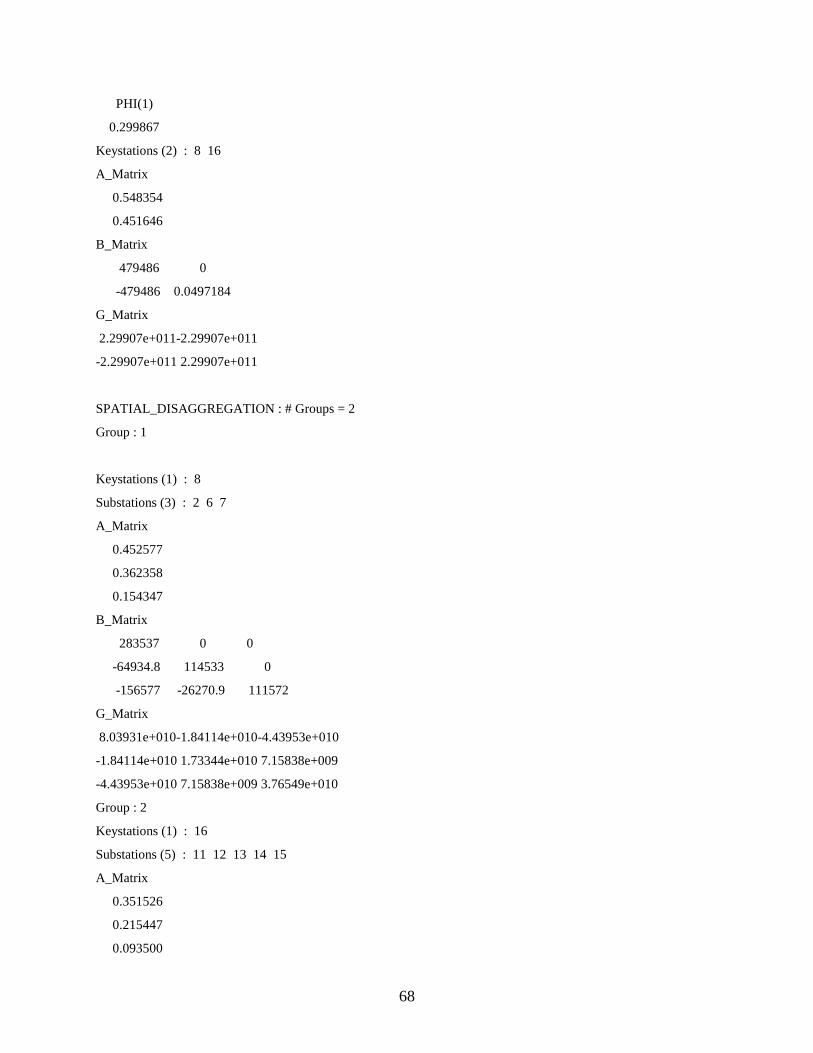
68
PHI(1)
0.299867
Keystations (2) : 8 16
A_Matrix
0.548354
0.451646
B_Matrix
479486 0
-479486 0.0497184
G_Matrix
2.29907e+011-2.29907e+011
-2.29907e+011 2.29907e+011
SPATIAL_DISAGGREGATION : # Groups = 2
Group : 1
Keystations (1) : 8
Substations (3) : 2 6 7
A_Matrix
0.452577
0.362358
0.154347
B_Matrix
283537 0 0
-64934.8 114533 0
-156577 -26270.9 111572
G_Matrix
8.03931e+010-1.84114e+010-4.43953e+010
-1.84114e+010 1.73344e+010 7.15838e+009
-4.43953e+010 7.15838e+009 3.76549e+010
Group : 2
Keystations (1) : 16
Substations (5) : 11 12 13 14 15
A_Matrix
0.351526
0.215447
0.093500
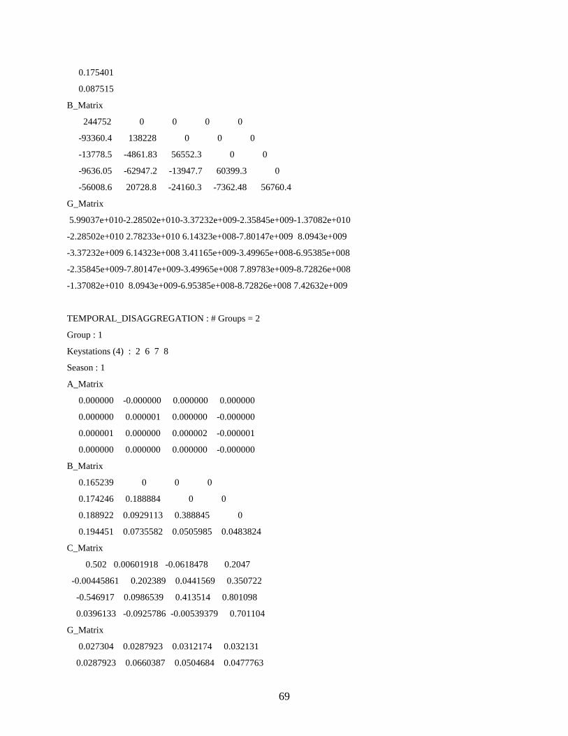
69
0.175401
0.087515
B_Matrix
244752 0 0 0 0
-93360.4 138228 0 0 0
-13778.5 -4861.83 56552.3 0 0
-9636.05 -62947.2 -13947.7 60399.3 0
-56008.6 20728.8 -24160.3 -7362.48 56760.4
G_Matrix
5.99037e+010-2.28502e+010-3.37232e+009-2.35845e+009-1.37082e+010
-2.28502e+010 2.78233e+010 6.14323e+008-7.80147e+009 8.0943e+009
-3.37232e+009 6.14323e+008 3.41165e+009-3.49965e+008-6.95385e+008
-2.35845e+009-7.80147e+009-3.49965e+008 7.89783e+009-8.72826e+008
-1.37082e+010 8.0943e+009-6.95385e+008-8.72826e+008 7.42632e+009
TEMPORAL_DISAGGREGATION : # Groups = 2
Group : 1
Keystations (4) : 2 6 7 8
Season : 1
A_Matrix
0.000000 -0.000000 0.000000 0.000000
0.000000 0.000001 0.000000 -0.000000
0.000001 0.000000 0.000002 -0.000001
0.000000 0.000000 0.000000 -0.000000
B_Matrix
0.165239 0 0 0
0.174246 0.188884 0 0
0.188922 0.0929113 0.388845 0
0.194451 0.0735582 0.0505985 0.0483824
C_Matrix
0.502 0.00601918 -0.0618478 0.2047
-0.00445861 0.202389 0.0441569 0.350722
-0.546917 0.0986539 0.413514 0.801098
0.0396133 -0.0925786 -0.00539379 0.701104
G_Matrix
0.027304 0.0287923 0.0312174 0.032131
0.0287923 0.0660387 0.0504684 0.0477763

70
0.0312174 0.0504684 0.195525 0.0632455
0.032131 0.0477763 0.0632455 0.0481231
Season : 2
A_Matrix
0.000000 0.000000 0.000000 -0.000000
-0.000000 0.000000 0.000000 -0.000000
0.000001 0.000001 0.000002 -0.000001
-0.000000 0.000000 0.000000 -0.000000
B_Matrix
0.115463 0 0 0
0.0683399 0.09938 0 0
0.191787 0.167487 0.515484 0
0.101526 0.0468169 0.0200979 0.0379594
C_Matrix
0.584598 0.295025 -0.0358156 -0.297984
0.195712 0.529944 -0.0559797 -0.104605
-1.11441 0.579704 -0.0267015 1.3718
0.101128 0.244169 -0.0635435 0.232122
G_Matrix
0.0133318 0.00789075 0.0221444 0.0117225
0.00789075 0.0145467 0.0297516 0.0115909
0.0221444 0.0297516 0.330558 0.0376727
0.0117225 0.0115909 0.0376727 0.0143442
Season : 3
A_Matrix
-0.000000 -0.000000 -0.000000 0.000000
0.000000 0.000000 0.000000 -0.000000
-0.000000 -0.000000 0.000001 0.000000
-0.000000 -0.000000 -0.000000 0.000000
B_Matrix
0.110573 0 0 0
0.0407358 0.117442 0 0
0.121705 0.14416 0.234975 0
0.0829946 0.0444141 0.0273941 0.0411484
C_Matrix
0.784109 0.221403 0.0265706 -0.251361
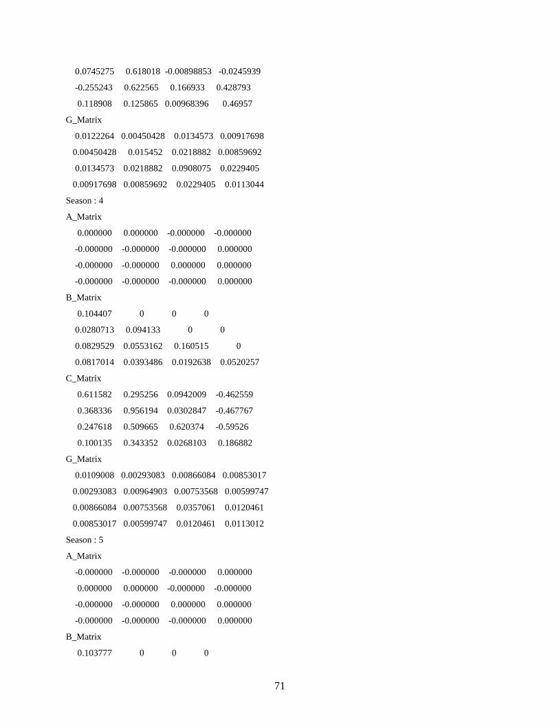
71
0.0745275 0.618018 -0.00898853 -0.0245939
-0.255243 0.622565 0.166933 0.428793
0.118908 0.125865 0.00968396 0.46957
G_Matrix
0.0122264 0.00450428 0.0134573 0.00917698
0.00450428 0.015452 0.0218882 0.00859692
0.0134573 0.0218882 0.0908075 0.0229405
0.00917698 0.00859692 0.0229405 0.0113044
Season : 4
A_Matrix
0.000000 0.000000 -0.000000 -0.000000
-0.000000 -0.000000 -0.000000 0.000000
-0.000000 -0.000000 0.000000 0.000000
-0.000000 -0.000000 -0.000000 0.000000
B_Matrix
0.104407 0 0 0
0.0280713 0.094133 0 0
0.0829529 0.0553162 0.160515 0
0.0817014 0.0393486 0.0192638 0.0520257
C_Matrix
0.611582 0.295256 0.0942009 -0.462559
0.368336 0.956194 0.0302847 -0.467767
0.247618 0.509665 0.620374 -0.59526
0.100135 0.343352 0.0268103 0.186882
G_Matrix
0.0109008 0.00293083 0.00866084 0.00853017
0.00293083 0.00964903 0.00753568 0.00599747
0.00866084 0.00753568 0.0357061 0.0120461
0.00853017 0.00599747 0.0120461 0.0113012
Season : 5
A_Matrix
-0.000000 -0.000000 -0.000000 0.000000
0.000000 0.000000 -0.000000 -0.000000
-0.000000 -0.000000 0.000000 0.000000
-0.000000 -0.000000 -0.000000 0.000000
B_Matrix
0.103777 0 0 0
72
0.0580655 0.1107 0 0
0.120727 0.111002 0.181246 0
0.0845675 0.0520657 0.0392643 0.0386531
C_Matrix
0.508873 0.22648 -0.0207566 0.004536
0.00822624 0.736931 -0.0270794 -0.0161657
-0.348239 0.307361 0.599449 -0.277384
-0.0927785 0.189521 0.064263 0.385511
G_Matrix
0.0107697 0.00602586 0.0125287 0.00877616
0.00602586 0.0156261 0.0192979 0.0106741
0.0125287 0.0192979 0.0597464 0.0231054
0.00877616 0.0106741 0.0231054 0.0128982
Season : 6
A_Matrix
-0.000000 -0.000000 0.000000 0.000000
-0.000000 0.000000 0.000000 -0.000000
-0.000000 -0.000000 0.000000 0.000000
-0.000000 -0.000000 -0.000000 0.000000
B_Matrix
0.131858 0 0 0
0.157242 0.1192 0 0
0.307016 0.167227 0.220716 0
0.169115 0.0640698 0.027466 0.0335856
C_Matrix
0.832518 0.516669 -0.18311 -0.326776
0.112288 1.35199 -0.216668 -0.359371
0.35402 1.41921 0.271095 -1.04644
0.306075 0.870295 -0.18714 -0.15756
G_Matrix
0.0173864 0.0207336 0.0404824 0.0222991
0.0207336 0.0389337 0.0682094 0.0342292
0.0404824 0.0682094 0.170939 0.0686975
0.0222991 0.0342292 0.0686975 0.0345873
Season : 7
A_Matrix
0.000000 0.000000 0.000000 -0.000000
73
0.000000 0.000001 0.000000 -0.000000
-0.000000 0.000000 0.000001 0.000000
-0.000000 0.000000 0.000000 -0.000000
B_Matrix
0.299458 0 0 0
0.355101 0.199638 0 0
0.278549 0.157015 0.266149 0
0.317119 0.112407 0.0616115 0.0401153
C_Matrix
0.261602 -0.738159 0.10459 1.0228
-0.314722 -0.758881 0.0986936 1.72177
-0.70911 -1.28352 0.240206 1.97092
-0.240315 -0.905514 0.0894443 1.66252
G_Matrix
0.0896748 0.106338 0.0834137 0.0949636
0.106338 0.165952 0.130259 0.13505
0.0834137 0.130259 0.173079 0.122381
0.0949636 0.13505 0.122381 0.118605
Season : 8
A_Matrix
0.000000 -0.000000 0.000000 -0.000000
0.000000 0.000001 -0.000000 -0.000000
-0.000000 0.000000 0.000001 0.000000
0.000000 0.000000 -0.000000 0.000000
B_Matrix
0.235985 0 0 0
0.186891 0.139408 0 0
0.095993 0.110841 0.144337 0
0.195934 0.0653626 0.0174017 0.0278394
C_Matrix
-0.214358 -0.0354761 -0.0495295 0.544537
-0.494318 0.0251764 0.183358 0.339971
-0.145423 0.214719 0.641238 -0.781904
-0.317377 0.0185208 0.118834 0.303672
G_Matrix
0.0556888 0.0441035 0.0226529 0.0462374

74
0.0441035 0.054363 0.0333924 0.0457304
0.0226529 0.0333924 0.0423335 0.0285648
0.0462374 0.0457304 0.0285648 0.0437401
Season : 9
A_Matrix
0.000001 -0.000001 0.000000 0.000000
0.000000 -0.000000 -0.000000 0.000000
0.000000 -0.000000 0.000000 0.000000
0.000000 -0.000000 0.000000 0.000000
B_Matrix
0.143215 0 0 0
0.131382 0.0852989 0 0
0.0904204 0.0745078 0.123244 0
0.134862 0.0353906 0.0102286 0.0146826
C_Matrix
-0.313999 1.0291 -0.00447895 -0.85982
-0.377288 1.13627 0.216743 -1.08805
0.140012 0.68938 0.640143 -1.54423
-0.408819 0.98173 0.0904113 -0.779671
G_Matrix
0.0205106 0.0188159 0.0129496 0.0193143
0.0188159 0.0245371 0.018235 0.0207372
0.0129496 0.018235 0.0289164 0.0160918
0.0193143 0.0207372 0.0160918 0.0197604
Season : 10
A_Matrix
0.000000 -0.000000 -0.000000 -0.000000
0.000000 -0.000000 -0.000000 0.000000
-0.000000 0.000000 -0.000000 0.000000
0.000000 -0.000000 -0.000000 0.000000
B_Matrix
0.196377 0 0 0
0.121377 0.117237 0 0
0.152896 0.0714537 0.15435 0
0.164305 0.0495302 0.00952933 0.022087
C_Matrix
1.02208 1.42797 0.358112 -2.34311
75
0.474762 1.74809 0.3798 -2.37985
1.82844 0.00808892 1.36039 -2.79386
0.58955 1.33452 0.35718 -1.92405
G_Matrix
0.0385639 0.0238356 0.0300253 0.0322657
0.0238356 0.0284769 0.0269351 0.0257496
0.0300253 0.0269351 0.0523067 0.0301316
0.0322657 0.0257496 0.0301316 0.0300281
Season : 11
A_Matrix
-0.000000 -0.000000 -0.000000 0.000000
0.000000 0.000000 -0.000000 -0.000000
-0.000000 0.000000 -0.000001 0.000000
-0.000000 -0.000000 -0.000000 0.000000
B_Matrix
0.154498 0 0 0
0.133507 0.126207 0 0
0.149137 0.111312 0.199762 0
0.153733 0.0615936 0.0215073 0.0245934
C_Matrix
1.53006 0.694829 0.184828 -2.00602
0.254645 0.490447 0.244753 -0.506946
0.636679 -0.364887 1.03079 -0.670124
0.567432 0.352455 0.215191 -0.671244
G_Matrix
0.0238695 0.0206265 0.0230413 0.0237514
0.0206265 0.0337523 0.0339591 0.028298
0.0230413 0.0339591 0.074537 0.0340797
0.0237514 0.028298 0.0340797 0.0284951
Season : 12
A_Matrix
-0.000000 -0.000000 -0.000000 0.000000
-0.000000 -0.000000 -0.000001 0.000000
-0.000000 -0.000000 -0.000000 0.000000
-0.000000 -0.000000 -0.000001 0.000000
B_Matrix
0.173759 0 0 0
76
0.206504 0.173242 0 0
0.259491 0.175559 0.18789 0
0.206645 0.0929467 0.0165958 0.0321004
C_Matrix
1.09253 0.991814 0.208764 -1.78649
1.11559 1.62944 0.462521 -2.57501
0.528264 1.12795 1.19301 -2.099
0.781725 1.0232 0.369226 -1.63444
G_Matrix
0.0301922 0.0358819 0.0450889 0.0359064
0.0358819 0.0726567 0.0840001 0.0587752
0.0450889 0.0840001 0.133459 0.0730583
0.0359064 0.0587752 0.0730583 0.052647
Group : 2
Keystations (6) : 11 12 13 14 15 16
Season : 1
A_Matrix
-0.000000 -0.000000 0.000000 -0.000000 0.000000 0.000000
-0.000000 -0.000000 0.000000 -0.000000 0.000000 0.000000
-0.000001 -0.000001 0.000002 -0.000000 0.000001 0.000000
-0.000001 -0.000001 0.000001 0.000000 0.000001 0.000000
-0.000000 -0.000000 0.000000 -0.000000 0.000001 0.000000
-0.000000 -0.000001 0.000000 -0.000000 0.000001 0.000000
B_Matrix
0.285005 0 0 0 0 0
0.147273 0.27085 0 0 0 0
0.20126 0.164535 0.415564 0 0 0
0.109297 0.186816 0.187282 0.340697 0 0
0.0578085 0.0919089 0.0436934 0.0166099 0.105877 0
0.154485 0.130975 0.0888181 0.083933 0.0169512 0.0682913
C_Matrix
0.847036 -0.139999 0.0169278 -5.119e-006 0.0499056 0.208286
-0.164877 0.492869 0.00705454-3.66774e-007 0.315733 0.0184223
-0.126584 -0.129972 0.366793-4.69759e-006 0.611799 0.434272
-0.0293906 0.332623 -0.0957983-1.97631e-006 -0.16423 0.954438
0.0467824 0.106837 -0.038057 5.9042e-007 0.493149 -0.204799
0.0806382 0.0993473 -0.0335549-3.75861e-006 0.127337 0.574945
77
G_Matrix
0.0812281 0.0419737 0.0573602 0.0311502 0.0164757 0.0440291
0.0419737 0.0950493 0.0742047 0.0666956 0.0334072 0.0582263
0.0573602 0.0742047 0.240271 0.130563 0.0449142 0.0895514
0.0311502 0.0666956 0.130563 0.197995 0.0373302 0.0865827
0.0164757 0.0334072 0.0449142 0.0373302 0.0251839 0.028038
0.0440291 0.0582263 0.0895514 0.0865827 0.028038 0.0609046
Season : 2
A_Matrix
0.000000 -0.000000 0.000000 -0.000001 0.000000 0.000000
0.000000 0.000000 -0.000001 -0.000000 0.000000 0.000000
-0.000000 -0.000001 0.000002 -0.000001 0.000000 0.000000
-0.000000 -0.000000 -0.000000 -0.000000 -0.000000 0.000000
0.000000 -0.000000 -0.000000 -0.000000 0.000000 0.000000
-0.000000 -0.000000 0.000000 -0.000001 0.000000 0.000000
B_Matrix
0.208608 0 0 0 0 0
0.0382309 0.130014 0 0 0 0
0.0986463 0.108202 0.436169 0 0 0
0.0443932 0.062832 0.0758254 0.179415 0 0
0.0196362 0.046147 0.018143 0.0264187 0.100145 0
0.0870833 0.0562514 0.0625358 0.052854 0.0303199 0.0555294
C_Matrix
0.525674 0.0310611 -0.0515085 -0.0540612 0.0659373 0.197631
0.0927287 0.538716 0.0192426 0.0312471 0.187425 -0.125084
-0.139031 -0.0131704 0.567466 -0.00831652 -0.545995 0.446387
0.0580618 -0.242813 -0.0438333 0.123865 0.0908805 0.678126
0.044274 0.0295561 -0.0462856 0.0572508 0.610288 -0.102927
0.114365 0.00689524 -0.0463633 0.0399899 0.0472178 0.454384
G_Matrix
0.0435174 0.00797528 0.0205784 0.00926079 0.00409628 0.0181663
0.00797528 0.0183654 0.0178392 0.00986626 0.00675048 0.0106428
0.0205784 0.0178392 0.211683 0.0442505 0.0148437 0.0419532
0.00926079 0.00986626 0.0442505 0.0438578 0.00988683 0.0216249
0.00409628 0.00675048 0.0148437 0.00988683 0.0135713 0.00987313
0.0181663 0.0106428 0.0419532 0.0216249 0.00987313 0.0214548
Season : 3
78
A_Matrix
-0.000000 -0.000001 -0.000000 -0.000001 0.000000 0.000000
0.000000 0.000000 0.000000 -0.000000 0.000000 -0.000000
0.000002 0.000001 0.000001 -0.000001 0.000001 -0.000001
-0.000000 -0.000001 -0.000001 -0.000001 -0.000001 0.000001
-0.000000 0.000000 -0.000000 -0.000000 -0.000001 0.000000
-0.000000 -0.000001 -0.000000 -0.000001 -0.000000 0.000001
B_Matrix
0.195419 0 0 0 0 0
0.0539538 0.171069 0 0 0 0
0.0647505 -0.0324771 0.661019 0 0 0
0.0287713 0.0661534 0.0271663 0.190175 0 0
0.0128477 0.0508977 0.0134093 0.0331178 0.154288 0
0.09405 0.0780211 0.0630443 0.0913526 0.0328096 0.112688
C_Matrix
0.619496 0.00333415 0.0118057 0.217456 0.0553685 -0.291704
0.198998 0.821329 0.0174582 0.077666 -0.0427117 -0.306024
-0.462329 0.215444 0.146556 0.478307 -1.06401 1.46074
0.43366 0.0531735 0.134351 0.622475 0.140597 -0.757733
0.290483 -0.0916578 0.0609616 0.0813061 1.16455 -0.582619
0.298901 0.138436 0.0623818 0.439362 0.197812 -0.386929
G_Matrix
0.0381888 0.0105436 0.0126535 0.00562248 0.00251068 0.0183792
0.0105436 0.0321755 -0.00206228 0.0128691 0.00940019 0.0184213
0.0126535 -0.00206228 0.442194 0.017672 0.00804268 0.0452293
0.00562248 0.0128691 0.017672 0.0421087 0.0103992 0.026953
0.00251068 0.00940019 0.00804268 0.0103992 0.027837 0.0141123
0.0183792 0.0184213 0.0452293 0.026953 0.0141123 0.0410277
Season : 4
A_Matrix
0.000000 -0.000000 0.000001 -0.000000 0.000000 -0.000000
0.000000 0.000000 0.000000 -0.000000 -0.000000 -0.000000
-0.000000 0.000001 -0.000002 -0.000000 -0.000003 0.000000
-0.000000 0.000000 -0.000000 0.000000 -0.000001 0.000000
0.000000 0.000000 -0.000001 0.000000 0.000000 -0.000000
-0.000000 0.000000 -0.000000 -0.000000 -0.000001 0.000000
79
B_Matrix
0.199906 0 0 0 0 0
0.0434595 0.15611 0 0 0 0
0.125496 0.0637498 0.645358 0 0 0
0.0517408 0.0502824 0.0530494 0.174034 0 0
0.0101648 0.0695764 0.0429212 0.017143 0.15085 0
0.0949124 0.0706154 0.0959296 0.0553493 0.0286384 0.112994
C_Matrix
0.456372 0.169639 0.0270982 0.173846 0.0719613 -0.297016
-0.0348421 0.647522 0.009666 -0.0626382 0.165722 0.0750104
0.214207 -0.130022 0.119922 0.0364644 0.1203 0.90666
0.134272 -0.177345 0.0595539 0.995467 0.123273 -0.38962
0.0579566 -0.0978169 0.0117883 -0.0598046 0.761261 0.0188213
0.0579642 0.0972999 0.0379637 0.0945716 0.212726 0.124871
G_Matrix
0.0399623 0.00868779 0.0250873 0.0103433 0.00203199 0.0189735
0.00868779 0.0262589 0.0154059 0.0100982 0.0113033 0.0151486
0.0250873 0.0154059 0.436301 0.0439346 0.0334106 0.0783218
0.0103433 0.0100982 0.0439346 0.0383074 0.0092848 0.0231832
0.00203199 0.0113033 0.0334106 0.0092848 0.0298362 0.0152643
0.0189735 0.0151486 0.0783218 0.0231832 0.0152643 0.0398487
Season : 5
A_Matrix
0.000000 -0.000000 -0.000000 -0.000000 0.000000 -0.000000
-0.000000 -0.000001 -0.000000 -0.000001 0.000001 0.000000
0.000000 -0.000002 0.000002 -0.000002 0.000001 0.000001
-0.000000 -0.000000 0.000000 -0.000000 0.000000 0.000000
0.000000 -0.000000 0.000000 -0.000000 0.000001 0.000000
-0.000000 -0.000001 0.000000 -0.000001 0.000000 0.000000
B_Matrix
0.159596 0 0 0 0 0
0.101062 0.167522 0 0 0 0
0.153032 0.0747625 0.570052 0 0 0
0.05178 0.0442827 0.0671975 0.158345 0 0
0.105814 0.0756747 0.0339011 0.0231095 0.160107 0
0.129943 0.07169 0.0955014 0.0431183 0.057536 0.106023
C_Matrix
80
0.685409 -0.076842 -0.0135456 0.0336975 -0.125412 0.0415845
0.00396154 0.717766 0.0280413 -0.148321 -0.139701 0.112067
-0.528005 0.689232 0.384568 0.469356 -0.743027 -0.280061
0.148998 0.147765 -0.0119671 0.712176 0.156593 -0.271624
-0.0556917 0.0836149 0.0118048 -0.0335969 0.474309 0.0363686
0.172447 0.192215 0.00116738 0.0776268 0.0232764 0.275925
G_Matrix
0.0254709 0.0161291 0.0244233 0.00826388 0.0168875 0.0207383
0.0161291 0.0382773 0.0279901 0.0126513 0.023371 0.025142
0.0244233 0.0279901 0.353968 0.0495408 0.0411759 0.0796859
0.00826388 0.0126513 0.0495408 0.0342309 0.0147675 0.0231481
0.0168875 0.023371 0.0411759 0.0147675 0.0442408 0.0326208
0.0207383 0.025142 0.0796859 0.0231481 0.0326208 0.0475555
Season : 6
A_Matrix
0.000000 -0.000000 0.000000 -0.000000 0.000001 -0.000000
0.000001 0.000001 0.000000 0.000001 0.000001 -0.000001
0.000001 -0.000000 0.000003 0.000001 0.000003 -0.000001
-0.000000 -0.000000 0.000000 0.000000 0.000000 0.000000
-0.000000 -0.000000 -0.000000 -0.000001 0.000001 0.000000
-0.000000 -0.000000 0.000000 -0.000001 0.000001 0.000000
B_Matrix
0.280219 0 0 0 0 0
0.19376 0.29 0 0 0 0
0.17493 0.159583 0.493805 0 0 0
0.0916778 0.0589661 0.0420819 0.188576 0 0
0.113837 0.0912975 0.00373795 0.066093 0.168548 0
0.194183 0.0937813 0.0610258 0.0839134 0.0383433 0.0764871
C_Matrix
0.740709 0.0601027 -0.0127117 0.0643772 -0.295936 -0.00685265
0.369643 0.800145 -0.0359232 0.241326 -0.436766 -0.175398
-0.0189178 0.0341422 0.09058 0.697201 -0.364466 -0.577036
0.27127 0.0339157 0.033778 0.486336 -0.0936392 -0.215272
0.124449 0.0720405 0.00407665 0.13609 0.0416237 -0.241706
0.391925 0.160908 -0.0189926 0.239589 -0.264417 -0.0780854
G_Matrix
0.0785225 0.0542952 0.0490187 0.0256898 0.0318993 0.0544137
81
0.0542952 0.121643 0.0801735 0.0348637 0.0485334 0.0648215
0.0490187 0.0801735 0.299911 0.0462274 0.0363288 0.0790691
0.0256898 0.0348637 0.0462274 0.0492137 0.0284407 0.0417243
0.0318993 0.0485334 0.0363288 0.0284407 0.0540847 0.0429041
0.0544137 0.0648215 0.0790691 0.0417243 0.0429041 0.064588
Season : 7
A_Matrix
0.000000 -0.000000 0.000001 0.000000 0.000001 -0.000000
-0.000000 0.000000 -0.000001 -0.000001 -0.000001 0.000001
-0.000000 0.000000 0.000002 0.000001 -0.000002 -0.000000
0.000000 0.000000 0.000001 0.000002 0.000000 -0.000000
-0.000000 -0.000000 0.000000 -0.000000 0.000002 -0.000000
-0.000000 -0.000000 0.000000 -0.000000 0.000000 0.000000
B_Matrix
0.265269 0 0 0 0 0
0.196505 0.264928 0 0 0 0
0.160227 0.0622116 0.736595 0 0 0
0.269947 0.17689 0.155451 0.279643 0 0
0.0878972 0.134956 0.039934 0.0325675 0.148683 0
0.214783 0.123925 0.0737765 0.035938 0.0249915 0.0579129
C_Matrix
0.390164 -0.0973805 -0.0221249 0.469146 0.385594 -0.503603
0.37239 0.365767 0.0127926 0.416421 0.48238 -0.884575
-0.387133 -0.229884 -0.19923 0.20542 -0.670378 2.05003
0.417304 -0.101802 0.0585601 0.835012 0.204766 -0.203654
0.258418 0.178543 -0.0361912 0.286109 0.264855 -0.544883
0.342412 0.0110104 -0.00740742 0.518697 0.28329 -0.456308
G_Matrix
0.0703676 0.0521266 0.0425032 0.0716086 0.0233164 0.0569752
0.0521266 0.108801 0.0479669 0.099909 0.0530259 0.075037
0.0425032 0.0479669 0.572116 0.168762 0.0518945 0.0964669
0.0716086 0.099909 0.168762 0.206527 0.062915 0.101419
0.0233164 0.0530259 0.0518945 0.062915 0.0507011 0.0434356
0.0569752 0.075037 0.0964669 0.101419 0.0434356 0.072202
Season : 8
A_Matrix
82
-0.000000 -0.000000 0.000000 -0.000001 -0.000000 0.000000
-0.000000 0.000001 -0.000000 -0.000000 -0.000000 0.000000
-0.000000 0.000001 0.000004 -0.000002 -0.000003 0.000000
0.000000 0.000001 0.000000 0.000001 0.000001 -0.000000
-0.000000 -0.000000 0.000000 -0.000000 0.000001 0.000000
-0.000000 -0.000000 -0.000000 -0.000001 -0.000000 0.000000
B_Matrix
0.237447 0 0 0 0 0
0.117654 0.124301 0 0 0 0
0.0251154 0.000878296 0.460776 0 0 0
0.306972 0.163429 0.00353014 0.314666 0 0
0.139078 0.137868 0.0132099 0.000165088 0.100435 0
0.171747 0.0985993 0.0193738 0.00415752 0.00879976 0.0506578
C_Matrix
0.837814 0.377201 0.0465612 0.172505 -0.0572134 -0.897734
0.347186 0.062265 0.0130696 0.0441428 -0.0311445 -0.312111
0.135354 -0.092551 0.22483 0.722157 0.0387132 -0.932959
0.826371 0.252456 0.111369 0.52824 -0.32659 -0.893197
0.357567 0.081522 0.0257244 0.030719 0.128037 -0.364023
0.481888 0.164018 0.0106008 0.114589 -0.0841181 -0.380957
G_Matrix
0.0563812 0.0279367 0.00596357 0.0728897 0.0330236 0.0407808
0.0279367 0.0292933 0.00306411 0.056431 0.0335003 0.0324628
0.00596357 0.00306411 0.212946 0.00947986 0.00970089 0.0133271
0.0728897 0.056431 0.00947986 0.219968 0.0653232 0.0702121
0.0330236 0.0335003 0.00970089 0.0653232 0.048612 0.0386203
0.0407808 0.0324628 0.0133271 0.0702121 0.0386203 0.0422551
Season : 9
A_Matrix
0.000001 -0.000000 0.000001 -0.000000 0.000000 -0.000000
0.000000 0.000000 0.000001 -0.000000 -0.000000 0.000000
0.000000 0.000000 0.000002 -0.000000 -0.000001 0.000000
0.000001 -0.000000 0.000001 0.000001 0.000000 0.000000
0.000000 -0.000000 0.000001 -0.000001 0.000001 0.000000
0.000000 -0.000000 0.000001 -0.000000 -0.000000 0.000000
B_Matrix
0.193892 0 0 0 0 0
83
0.142062 0.162094 0 0 0 0
0.187929 0.0846477 0.315797 0 0 0
0.226906 0.109477 0.0015968 0.157789 0 0
0.139317 0.167067 -0.0173124 0.0075406 0.106178 0
0.164551 0.0788464 0.0270704 0.0148108 0.0205552 0.0349233
C_Matrix
-0.335414 0.690554 -0.0471818 0.136273 -0.123464 -0.379109
-0.0990891 1.21683 -0.00647378 0.212881 -0.338529 -1.06975
-0.306851 0.59397 0.0330352 0.209438 0.21707 -0.698624
-0.464655 0.727712 -0.0536591 0.485781 -0.251305 -0.753889
0.0894981 1.03736 0.00456233 0.138789 0.00734894 -1.12235
-0.182701 0.877611 -0.0295626 0.147414 -0.123517 -0.674348
G_Matrix
0.0375941 0.0275448 0.036438 0.0439952 0.0270125 0.0319052
0.0275448 0.0464562 0.0404186 0.0499804 0.0468723 0.0361571
0.036438 0.0404186 0.14221 0.0524135 0.0348564 0.046147
0.0439952 0.0499804 0.0524135 0.0883713 0.0510641 0.0483498
0.0270125 0.0468723 0.0348564 0.0510641 0.0589509 0.037923
0.0319052 0.0361571 0.046147 0.0483498 0.037923 0.0358882
Season : 10
A_Matrix
-0.000000 -0.000000 -0.000001 -0.000000 -0.000001 0.000000
0.000000 0.000000 -0.000001 -0.000000 -0.000000 0.000000
-0.000001 -0.000000 0.000002 0.000001 -0.000000 0.000000
0.000000 0.000000 -0.000001 0.000002 -0.000001 -0.000000
0.000000 0.000000 -0.000001 0.000000 0.000001 -0.000000
0.000000 -0.000000 -0.000000 0.000000 -0.000000 0.000000
B_Matrix
0.231415 0 0 0 0 0
0.18348 0.192806 0 0 0 0
0.0858458 0.0396418 0.473277 0 0 0
0.166964 0.0390491 0.0485683 0.20094 0 0
0.0962816 0.129922 0.0346361 -0.00264773 0.124188 0
0.175676 0.0585303 0.0678499 0.0138436 0.0227715 0.0356419
C_Matrix
0.755708 0.63039 0.0197041 0.247076 -0.188985 -1.16575
-0.492869 1.12112 0.0271109 0.171024 -0.338696 -0.000672795
84
0.826359 0.209297 -0.678656 0.11915 0.390772 0.00750674
0.441224 0.704869 0.0660505 0.593249 -0.0460397 -1.38818
-0.473111 0.265123 -0.030752 0.136676 0.0250877 0.315268
0.213091 0.533318 -0.114337 0.161619 -0.134471 -0.281703
G_Matrix
0.0535528 0.0424599 0.019866 0.038638 0.022281 0.0406541
0.0424599 0.0708391 0.0233941 0.0381635 0.0427155 0.043518
0.019866 0.0233941 0.232933 0.0388674 0.0298082 0.0495131
0.038638 0.0381635 0.0388674 0.0721378 0.0222991 0.0376943
0.022281 0.0427155 0.0298082 0.0222991 0.0427792 0.0296601
0.0406541 0.043518 0.0495131 0.0376943 0.0296601 0.040872
Season : 11
A_Matrix
0.000000 -0.000000 -0.000000 -0.000000 0.000001 -0.000000
0.000000 0.000000 0.000000 0.000001 0.000000 -0.000000
0.000000 0.000000 -0.000001 0.000001 0.000001 -0.000000
0.009591 -0.001738 -0.022736 0.008301 0.022775 0.000608
0.000000 0.000000 -0.000000 0.000001 0.000001 -0.000000
0.000000 -0.000000 -0.000000 0.000000 0.000001 -0.000000
B_Matrix
0.153232 0 0 0 0 0
0.081007 0.153844 0 0 0 0
0.0477256 0.0127606 0.308689 0 0 0
4767 3245.48 2403.21 11667.1 0 0
0.0410478 0.0728789 0.0370756 0.0088064 0.10552 0
0.118075 0.0533969 0.0411878 0.0327145 0.0251705 0.0521391
C_Matrix
0.415481 0.225944 0.0365169 0.18394 -0.0204386 -0.492665
0.279419 0.473847 -0.111407 -0.0173875 -0.00543361 -0.318024
0.730571 -0.318439 1.34745 0.211189 0.777978 -1.98934
-12991.4 -4032.34 1687.79 38543.1 -16578.6 5307.71
0.289613 0.0722257 0.161461 0.0238898 0.383126 -0.657843
0.179116 0.0568042 0.116174 0.171603 0.0491121 -0.205721
G_Matrix
0.0234801 0.0124129 0.00731309 730.458 0.00628984 0.0180929
0.0124129 0.0302301 0.00582925 885.458 0.0145371 0.0177797
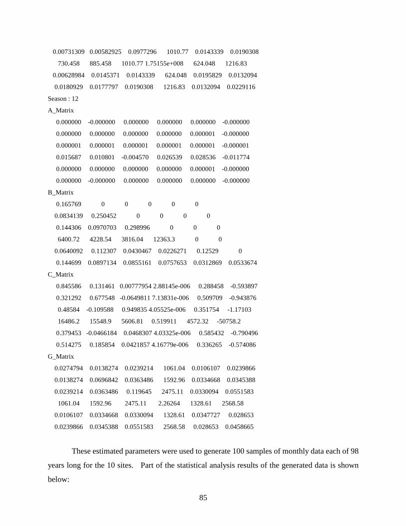
85
0.00731309 0.00582925 0.0977296 1010.77 0.0143339 0.0190308
730.458 885.458 1010.77 1.75155e+008 624.048 1216.83
0.00628984 0.0145371 0.0143339 624.048 0.0195829 0.0132094
0.0180929 0.0177797 0.0190308 1216.83 0.0132094 0.0229116
Season : 12
A_Matrix
0.000000 -0.000000 0.000000 0.000000 0.000000 -0.000000
0.000000 0.000000 0.000000 0.000000 0.000001 -0.000000
0.000001 0.000001 0.000001 0.000001 0.000001 -0.000001
0.015687 0.010801 -0.004570 0.026539 0.028536 -0.011774
0.000000 0.000000 0.000000 0.000000 0.000001 -0.000000
0.000000 -0.000000 0.000000 0.000000 0.000000 -0.000000
B_Matrix
0.165769 0 0 0 0 0
0.0834139 0.250452 0 0 0 0
0.144306 0.0970703 0.298996 0 0 0
6400.72 4228.54 3816.04 12363.3 0 0
0.0640092 0.112307 0.0430467 0.0226271 0.12529 0
0.144699 0.0897134 0.0855161 0.0757653 0.0312869 0.0533674
C_Matrix
0.845586 0.131461 0.00777954 2.88145e-006 0.288458 -0.593897
0.321292 0.677548 -0.0649811 7.13831e-006 0.509709 -0.943876
0.48584 -0.109588 0.949835 4.05525e-006 0.351754 -1.17103
16486.2 15548.9 5606.81 0.519911 4572.32 -50758.2
0.379453 -0.0466184 0.0468307 4.03325e-006 0.585432 -0.790496
0.514275 0.185854 0.0421857 4.16779e-006 0.336265 -0.574086
G_Matrix
0.0274794 0.0138274 0.0239214 1061.04 0.0106107 0.0239866
0.0138274 0.0696842 0.0363486 1592.96 0.0334668 0.0345388
0.0239214 0.0363486 0.119645 2475.11 0.0330094 0.0551583
1061.04 1592.96 2475.11 2.26264 1328.61 2568.58
0.0106107 0.0334668 0.0330094 1328.61 0.0347727 0.028653
0.0239866 0.0345388 0.0551583 2568.58 0.028653 0.0458665
These estimated parameters were used to generate 100 samples of monthly data each of 98
years long for the 10 sites. Part of the statistical analysis results of the generated data is shown
below:
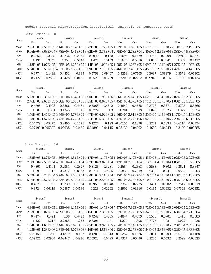
86
Model: Seasonal Disaggregation,(Statistical Analysis of Generated Data) Site Number: 8
Season 1 Season 2 Season 3 Season 4 Season 5 Season 6 Stats
Hist. Gen Hist. Gen Hist. Gen Hist. Gen Hist. Gen Hist. Gen
Mean 2.55E+05 2.55E+05 2.14E+05 2.14E+05 1.77E+05 1.77E+05 1.62E+05 1.62E+05 1.57E+05 1.57E+05 2.19E+05 2.19E+05StDev 9.06E+04 8.63E+04 4.78E+04 4.46E+04 3.62E+04 3.35E+04 2.75E+04 2.73E+04 2.80E+04 2.69E+04 6.38E+04 5.88E+04
CV 0.3556 0.3358 0.2236 0.2075 0.2042 0.188 0.1696 0.1679 0.1782 0.1708 0.2912 0.2671Skew 1.191 0.9443 1.354 0.5748 1.425 0.5139 0.5625 0.5076 0.88780.4841 1.369 0.7417Min 1.13E+05 1.07E+05 1.05E+05 1.25E+05 1.14E+05 1.09E+05 1.08E+05 1.06E+05 1.09E+05 1.01E+05 1.27E+05 1.09E+05Max 5.84E+05 5.56E+05 4.07E+05 3.53E+05 3.09E+05 2.79E+05 2.46E+05 2.45E+05 2.45E+05 2.39E+05 4.47E+05 4.14E+05acf(1) 0.1774 0.1439 0.4452 0.115 0.5758 0.09407 0.5258 0.07505 0.3037 0.08979 0.3578 0.06902acf(2) 0.2127 0.02867 0.3428 0.0125 0.3529 0.01799 0.2203 0.002252 0.09943 0.016 0.1786 0.02124
Season 7 Season 8 Season 9 Season 10 Season 11 Season 12 Stats
Hist. Gen Hist. Gen Hist. Gen Hist. Gen Hist. Gen Hist. Gen
Mean 5.23E+05 5.30E+05 1.51E+06 1.54E+06 1.90E+06 1.93E+06 9.56E+05 9.64E+05 4.62E+05 4.64E+05 2.87E+05 2.88E+05StDev 2.46E+05 2.63E+05 5.88E+05 6.99E+05 7.35E+05 8.87E+05 4.45E+05 4.57E+05 1.71E+05 1.67E+05 1.09E+05 1.03E+05
CV 0.4708 0.4908 0.3886 0.4481 0.3868 0.4542 0.4649 0.4688 0.3707 0.3571 0.3793 0.3566Skew 1.007 1.381 0.4345 1.317 0.3724 1.3 1.201 1.319 1.046 1.025 1.372 1.054Min 1.56E+05 1.47E+05 3.44E+05 4.79E+05 4.47E+05 6.02E+05 2.86E+05 2.91E+05 1.95E+05 1.83E+05 1.17E+05 1.15E+05Max 1.38E+06 1.57E+06 3.42E+06 4.26E+06 3.71E+06 5.30E+06 2.47E+06 2.74E+06 1.02E+06 1.06E+06 7.29E+05 6.61E+05acf(1) 0.07579 0.05275 0.2495 0.1621 0.1226 0.193 -0.00155 0.18980.1201 0.1694 0.06114 0.08354acf(2) 0.07499 0.005327 -0.05038 0.04425 0.04898 0.04115 0.081380.04902 0.1682 0.04849 0.3109 0.005685
Site Number: 16
Season 1 Season 2 Season 3 Season 4 Season 5 Season 6 Stats
Hist. Gen Hist. Gen Hist. Gen Hist. Gen Hist. Gen Hist. Gen
Mean 1.83E+05 1.82E+05 1.56E+05 1.56E+05 1.17E+05 1.17E+05 1.20E+05 1.19E+05 1.43E+05 1.42E+05 2.92E+05 2.92E+05StDev 7.88E+04 7.50E+04 4.61E+04 4.53E+04 3.67E+04 3.82E+04 3.17E+04 3.19E+04 5.13E+04 4.31E+04 1.06E+05 1.07E+05
CV 0.4301 0.4101 0.2951 0.2897 0.3126 0.3231 0.2654 0.2663 0.3583 0.302 0.3621 0.3647Skew 1.293 1.17 0.7312 0.8623 0.5711 0.9595 0.5839 0.7619 2.335 0.941 0.9584 1.003Min 5.49E+04 6.20E+04 5.74E+04 7.52E+04 4.60E+04 5.11E+04 6.15E+04 5.97E+04 6.16E+04 6.63E+04 1.18E+05 1.13E+05Max 5.06E+05 4.57E+05 2.83E+05 3.10E+05 2.25E+05 2.54E+05 2.09E+05 2.25E+05 4.10E+05 2.93E+05 7.03E+05 6.70E+05acf(1) 0.4071 0.1962 0.3239 0.1574 0.3953 0.09348 0.3352 0.07235 0.1401 0.07302 0.2517 0.09619acf(2) 0.3724 0.06119 0.2887 0.04546 0.228 0.02202 0.2902 0.018160.0185 0.01632 0.07323 0.02852
Season 7 Season 8 Season 9 Season 10 Season 11 Season 12 Stats
Hist. Gen Hist. Gen Hist. Gen Hist. Gen Hist. Gen Hist. Gen
Mean 4.86E+05 4.88E+05 1.13E+06 1.15E+06 1.45E+06 1.47E+06 7.57E+05 7.62E+05 3.72E+05 3.74E+05 2.09E+05 2.08E+05StDev 2.03E+05 2.07E+05 4.29E+05 5.11E+05 6.15E+05 7.39E+05 3.67E+05 3.77E+05 1.34E+05 1.39E+05 8.68E+04 7.71E+04
CV 0.4174 0.421 0.38 0.4423 0.4242 0.4965 0.4844 0.4899 0.35860.3701 0.415 0.3683Skew 1.122 1.217 0.2865 1.238 0.5391 1.471 1.277 1.398 0.7773 1.081 2.022 1.038Min 1.84E+05 1.65E+05 2.44E+05 3.62E+05 2.85E+05 3.92E+05 2.04E+05 2.14E+05 1.51E+05 1.45E+05 8.70E+04 7.99E+04Max 1.23E+06 1.28E+06 2.31E+06 3.07E+06 3.16E+06 4.51E+06 2.12E+06 2.27E+06 7.84E+05 8.85E+05 6.32E+05 4.83E+05acf(1) 0.08158 0.1085 0.1879 0.157 0.1286 0.1813 0.05257 0.1676 0.2001 0.1709 0.06152 0.1188acf(2) 0.09421 0.02964 0.02447 0.04916 0.05923 0.0495 0.07317 0.05436 0.1285 0.0532 0.2599 0.03823
87
REFERENCES Boswell, M.T., Ord, J.K., and Patil, G.P., 1979. Normal and lognormal distributions as models of
size. Statistical Distributions in Ecological Work, J.K. Ord, G.P. Patil and C.Taillie (editors), 72-87, Fairland, MD: International Cooperative Publishing House.
Brockwell, P.J. and Davis, R.A., 1996. Introduction to Time Series and Forecasting. Springer Texts in Statistics. Springer-Verlag, first edition.
Fernandez, B., and J.D. Salas, 1990, Gamma-Autoregressive Models for Stream-Flow Simulation, ASCE Journal of Hydraulic Engineering, vol. 116, no. 11, pp. 1403-1414.
Filliben, J.J., 1975. The probability plot correlation coefficient test for normality. Technometrics, 17(1):111–117.
Frevert, D.K., M.S. Cowan, and W.L. Lane, 1989, Use of Stochastic Hydrology in Reservoir Operation, J. Irrig. Drain. Eng., 115(3), pp. 334-343.
Gill, P E., W. Murray, and M.H. Wright, 1981, Practical Optimization, Academic Press, N. York. Grygier, J.C., and Stedinger, J.R., 1990., “SPIGOT, A Synthetic Streamflow Generation Software
Package”, technical description, version 2.5, School of Civil and Environmental Engineering, Cornell University, Ithaca, N.Y.
Himmenlblau, D.M., 1972, Applied Nonlinear Programming, McGraw-Hill, New York. Hipel, K. and McLeod, A.I. 1994. "Time Series Modeling of Water Resources and Environmental
Systems", Elsevier, Amsterdam, 1013 pages. Hurvich, C.M. and Tsai, C.-L., 1989. Regression and time series model selection in small samples.
Biometrika, 76(2):297–307. Hurvich, C.M. and Tsai, C.-L., 1993. A corrected Akaike information criterion for vector
autoregressive model selection. J. Time Series Anal. 14, 271–279. Kendall, M.G., 1963, The advanced theory of statistics, vol. 3, 2nd Ed., Charles Griffin and Co. Ltd.,
London, England. Lane, W.L., 1979, Applied Stochastic Techniques (Last Computer Package); User Manual, Division
of Planning Technical Services, U.S. Bureau of Reclamation, Denver, Colo. Lane, W.L., 1981, Corrected Parameter Estimates for Disaggregation Schemes, Inter. Symp. On
Rainfall Runoff Modeling, Mississippi State University. Lane, W.L., and D.K. Frevert, 1990, Applied Stochastic Techniques, personal computer version 5.2,
users manual, Bureau of Reclamation, U.S. Dep. of Interior, Denver, Colorado. Lawrance, A.J., 1982, The innovation distribution of a gamma distributed autoregressive process,
Scandinavian J. Statistics, 9(4), 234-236. Lawrance, A.J. and P. A. W. Lewis, 1981, A New Autoregressive Time Series Model in Exponential
Variables [NEAR(1)], Adv. Appl. Prob., 13(4), pp. 826-845. Loucks, D.P., J.R. Stedinger, and D.A. Haith, 1981, Water Resources Systems Planning and
Analysis, Prentice-Hall, Englewood Cliffs, N.J.. Matalas, N.C., 1966, Time Series Analysis, Water Resour. Res., 3(4), pp. 817-829. Mejia, J.M. and Rousselle, J., 1976. Disaggregation Models in Hydrology Revisited. Water
Resources Research, 12(3):185-186. O’Connell, P.E., 1977, ARIMA Models in Synthetic Hydrology, Mathematical Models for Surface
Water Hydrology, in T. Ciriani, V. Maione, and J. Wallis, eds., Wiley & Sons, N. Y., 51-68. Valencia, R.D. and Schaake Jr, J.C., 1973. Disaggregation Processes in Stochastic Hydrology.
Water Resources Research, 9(3):580-585. Salas, J.D., Delleur, J.W., Yevjevich, V., and Lane, W.L., 1980. Applied Modeling of Hydrologic
Time Series. Water Resources Publications, Littleton, CO, USA, first edition. Fourth printing,
88
1997. Salas, J.D., 1993. Analysis and Modeling of Hydrologic Time Series, chapter 19. Handbook of
Hydrology. McGraw-Hill. Salas, J.D., Saada, N., Chung, C.H., Lane, W.L. and Frevert, D.K., 2000, “Stochastic Analysis,
Modeling and Simulation (SAMS) Version 2000 - User’s Manual”, Colorado State University, Water Resources Hydrologic and Environmental Sciences, Technical Report Number 10, Engineering and Research Center, Colorado State University, Fort Collins, Colorado.
Shumway, R.H. and Stoffer, D.S., 2000. Time Series Analysis and Its Applications. Springer Texts in Statistics. Springer-Verlag, first edition.
Snedecor, G.W. and Cochran, W.G., 1980. Statistical Methods. Iowa State University Press, Iowa, seventh edition.
Salas, J.D., 1993, Analysis and Modeling of Hydrologic Time Series, Handbook of Hydrology, Chap. 19, pp.19.1-19.72, edited by D.R. Maidment, McGraw-Hill, Inc., New York.
Salas, J.D., D.C. Boes, and R.A. Smith, 1982, Estimation of ARMA Models with Seasonal Parameters, Water Resources Res., vol. 18, no. 4, pp. 1006-1010.
Salas, J.D., et al, 1999, Statistical Computer Techniques for Water Resources and EnvironmentalEngineering, forthcoming book.
Salas, J. D., J. W. Delleur, V. Yevjevich, and W. L. Lane, 1980, Applied Modeling of Hydrologic Time Series, WWP, Littleton, Colorado.
Stedinger, J.R., Vogel, R.M, and Foufoula-Georgiu, E., 1993. Analysis and Modeling of Hydrologic Time Series, chapter 18. Handbook of Hydrology. McGraw-Hill.
Stedinger, J. R., D. P. Lettenmaier and R. M. Vogel, 1985, Multisite ARMA(1,1) and Disaggregation Models for Annual Stream flow Generation, Water Resour. Res., 21(4), pp. 497-509.
Sveinsson, O.G.B., 2004, “Unequal Record Lengths in SAMS”, technical report resulting from work on multivariate shifting mean models for the Great Lakes. Work done for the International Joint Commission of Canada & United States.
Sveinsson, O.G.B., and Salas, J.D. 2006: Multivariate Shifting Mean Plus Persistence Model for Simulating the Great Lakes Net Basin Supplies. Proceedings of the 26th AGU Hydrology Days, Colorado State University, 173-184.
Sveinsson, O. G. B., Salas, J. D., Boes, D. C., and R. A. Pielke Sr., 2003: Modeling the dynamics of long term variability of hydroclimatic processes. Journal of Hydrometeorology, 4:489-505.
Sveinsson, O. G. B., Salas, J. D., and D. C. Boes, 2005: Prediction of extreme events in Hydrologic Processes that exhibit abrupt shifting patterns. Journal of Hydrologic Engineering, 10(4):315-326.
U. S. Army Corps of Engineers, 1971, HEC-4 Monthly Streamflow Simulation, Hydrologic Engineering Center, Davis, Calif..
Valencia, D., and J. C. Schaake, Jr., 1973, Disaggregation Processes in Stochastic Hydrology, Water Resources Research, vol. 9, no. 3, pp.580-585
89
APPENDIX A: PARAMETER ESTIMATION AND GENERATION
A.1 Transformation
A.1.1 Tests of Normality
Two normality tests are used in SAMS, namely the skewness test of normality (Snedecor and
Cochran, 1980) and Filliben probability plot correlation test (Filliben, 1975) both applied at the 10%
significance level. Both tests can be applied on an annual or seasonal basis.
In the skewness test of normality we assume a sample { } ( )21 ,N~ XX
Ntt iidX σµ= . Then the
estimated sample skewness from Eq. (3.3) g is asymptotically distributed as ( )N/6,0N 2 =σ . The
null hypothesis H0: g = 0 vs H1: g ≠ 0 is rejected at the α significance level if abs(g) > Nz /6/2-1α ,
where zq is the qth quantile from the standard normal distribution. According to Snedecor and
Cochran (1980) the above probability limits are accurate for sample sizes greater than 150, for
smaller sample sizes tabulated test statistics are given for example in Salas et al. (1980).
For a random sample X1, X2,…, XN of size N the Filliben probability plot correlation
coefficient test of normality is applied on the cross correlation coefficient R0(Xi:N Mi:N) where the
sample correlation coefficient is calculated by Eq. (3.4), Xi:N is the ith sample order statistic and Mi:N
is the ith order statistic median from a standard normal distribution. Mi:N is estimated as F-1(ui:N)
where F-1 is the inverse of the standard normal cumulative distribution function and ui:N is the order
statistic median from the uniform U(0; 1) distribution estimated as u1:N = (1-2-1/N), ui:N = (i –
0.3175)/(N + 0.365 ) for i = 2,…,N – 1, and uN:N = 2-1/N. The null hypothesis H0: r0 = 1 vs H1: r0 < 1
is rejected at the α significance level if r0 < ρα(N) where ρα(N) is a tabulated test statistic given in
Filliben (1975) and Vogel (1986) for the above plotting position. Johnson and Wichern (2002, page
182) give tabulated test statistics for the case when ui:N is estimated based on the Hazen plotting
position.
A.1.2 Automatic Transformation
The user can select to have SAMS select the best transformation or to have SAMS suggest a
Logarithmic, Power and Gamma transformation. The parameters of the transformations are
estimated in the following way when “Auto” transformation button is selected:
Logarithmic: The location parameter a of Eq. (4.1) is estimated based on a method suggested by
Boswell et al. (1979), with )2/()( :2/maxmin2
:2/maxmin NNNN xxxxxxa −+−= , where NNx :2/ is the
90
median of the sample series.
Gamma: The Wilson-Hilferty transformation (Loucks et al., 1981), is used for transforming a
Gamma variate to a normal variate.
Power: The parameters of the Power transformation is Eq. (4.3) are estimated by an iterative
process aimed at maximizing the Filliben correlation coefficient test statistic.
When the “Best Transf” button is pressed then SAMS chooses the best transformation among
Normal, Logarithmic with a = 0 (LN-2), Logarithmic with a estimated as above (LN-3), Gamma,
and if the sample skewness is negative the Power transformation is also used. The transformation
resulting in the highest adjusted Filliben correlation coefficient test statistic is selected as the best
one. The Filliben test statistic is slightly penalized for the LN-3, since the simpler LN-2 or Normal
should be preferred if the test statistics are similar. In addition, the Gamma and the Power are slightly
penalized over the LN-3. Due to this penalization, the distribution with the highest Filliben test
statistic may not be selected as the best one.
A.2 Parameter Estimation of Univariate Models
A.2.1 Univariate ARMA(p,q)
The method of moments (MOM) and Least Squares (LS) method can be used for estimation of
the parameters of the ARMA(p,q) model in chapter 4, Eq. (4.6). The MOM method is equivalent to
Yule-Walker estimation in Brockwell and Davis (1996). For example, the moment estimators for the
ARMA (1,0) , ARMA (1,1) and ARMA (2,1) models are given as:
- ARMA (1,0) model:
ttt YY εφ += −11 (A.1)
11 r=φ (A.2)
)ˆ1()(ˆ 21
22 φεσ −= s (A.3)
- ARMA (1,1) model:
1111 −− −+= tttt YY εθεφ (A.4)
1
21 r
r=φ (A.5)
111
1111 ˆ
1ˆ
ˆ1ˆˆθφ
φφθ −−
−+=
r
r (A.6)
91
1
1122
ˆ
ˆ)(ˆ
θφεσ r
s−
= (A.7)
where 1θ is estimated by solving Eq. (A.6).
- ARMA (2,1) model:
112211 −−− −++= ttttt YYY εθεφφ (A.8)
2
21
3121
rr
rrr
−−
=φ (A.9)
1
2132
ˆˆ
r
rr φφ −= (A.10)
11211
1211
1211
221111 ˆ)ˆˆ(
ˆˆ
ˆˆ
ˆˆ1ˆˆθφφ
φφφφφφφθ
rr
rr
rr
rr
+−+−
−+−−−
+= (A.11)
1
112122
ˆ
ˆˆ)(ˆ
θφφεσ rr
s−+
= (A.12)
where s2 is the variance of Yt and rk = mk / s2 is the estimate of the lag-k autocorrelation coefficient of
Yt which is defined as Rk = E[Yt Yt-k] / E[Yt Yt]. Similarly mk is the estimate of the lag-k
autocovariance coefficient of Yt with Mk = E[Yt Yt-k]. In the foregoing model it is assumed that the
mean has been removed or E[Yt] = 0. Note also that s2 = m0.
The Least Squares (LS) method is generally a more efficient parameter estimation method. In
this method, the parameters φ’s and θ’s are estimated by minimizing the sum of squares of the
residuals defined by
∑=
=N
ttF
1
2ε (A.13)
where N is the number of years of data. For the ARMA(p,q) model, the residuals are defined as
∑∑=
−=
− +−=q
jjtj
p
iititt YY
11
εθφε (A.14)
Once the φ’s and θ’s are determined, then the noise variance σ2(ε) is determined by ∑ =N
t tN1
2)/1( ε .
The minimization of the sum of squares of Eq. (A.13) may be obtained by a numerical scheme. In
SAMS first a high order AR(p) model is fitted to the data to get initial estimate of the noise terms tε .
Then iteratively a regression model is fitted to the data and the parameters φ’s and θ’s are re-
92
estimated and the residuals are re-calculated until the sum of the squares of the residuals has
converged to a minimum value.
To generate synthetic series from an ARMA model, Eq. (4.6) can be used. The white noise
process is generated by first generating a standard uncorrelated normal random variable zt and then
calculating εt as
tt z)(εσε = (A.15)
For generation of the correlated series Yt, a warm-up procedure is followed. In this procedure, values
of Yt prior to t = 1 are assumed to be equal to the mean of the process (which is zero in this case).
Thus, Y1 , Y2 , . . . , YN+L are generated using Eq. (4.6) by generating ε1-q , ε2-q , ε3-q , ... from Eq. (A.15)
where N is the required length to be generated and L is the warm-up length required to remove the
effect of the initial assumptions of Yt . L is arbitrarily chosen as 50 in SAMS. The advantage of the
warm up procedure is that it can be used for low order and high order stationary and periodic models
while exact generation procedures available in the literature apply only for stationary ARMA models
or the low order periodic models.
A.2.2 Univariate GAR(1)
The stationary GAR(1) process of Eq. (4.7) has four parameters {φ, λ, α, β}. It may be
shown that the relationships between the model parameters and the population moments of the
underlying variableX t are:
αβλµ += (A.16)
22
αβσ = (A.17)
β
γ 2= (A.18)
φρ =1 (A.19)
where µ, σ2, γ and ρ1 are the mean, variance, skewness coefficient, and the lag-one autocorrelation
coefficient, respectively.
Estimation of the parameters of the GAR(1) model is based on results by Kendall (1968),
Wallis and O’Connell (1972), and Matalas (1966) and based on extensive simulation experiments
conducted by Fernandez and Salas (1990). These studies suggest the following estimation procedure
for the four parameters {φ, λ, α, β}. First the sample moments are corrected to ensure unbiased
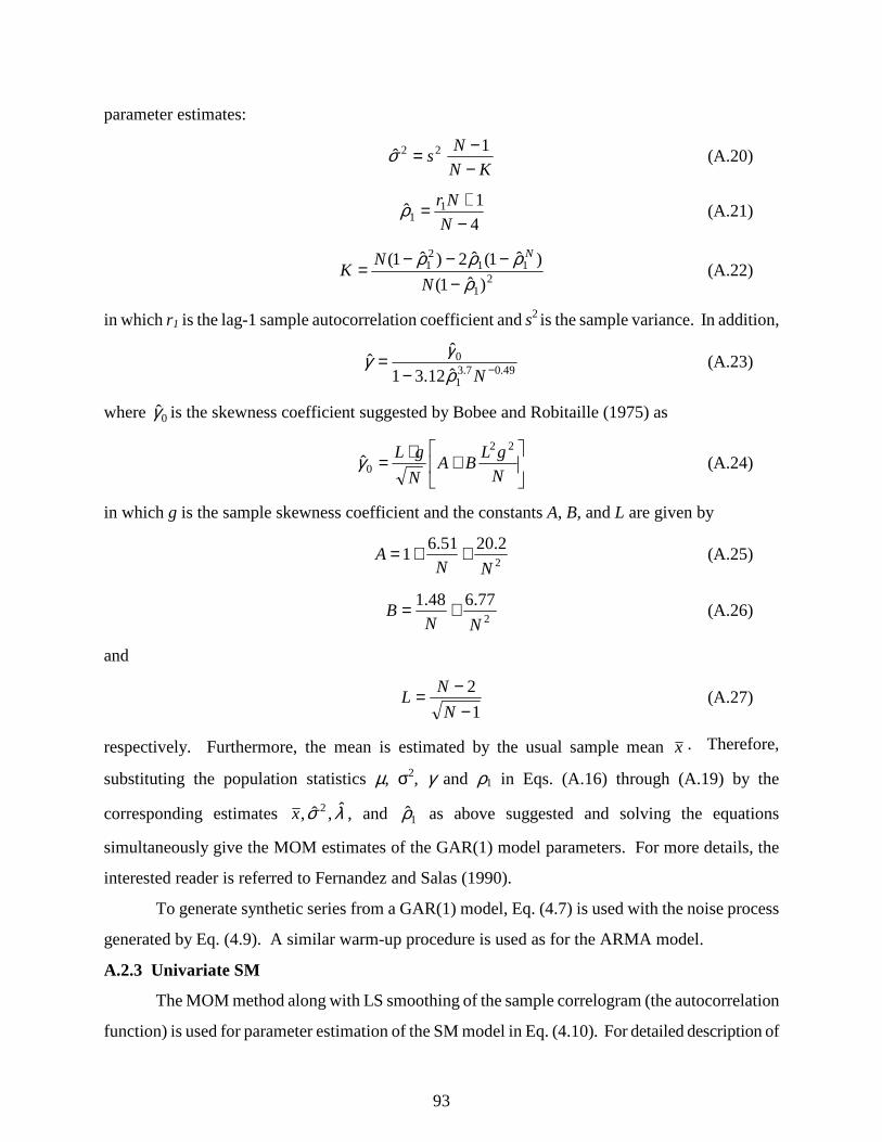
93
parameter estimates:
KN
Ns
−−= 1
ˆ 22σ (A.20)
4
1ˆ 11 −
+=N
Nrρ (A.21)
2
1
1121
)ˆ1(
)ˆ1(ˆ2)ˆ1(
ρρρρ
−−−−=
N
NK
N
(A.22)
in which r1 is the lag-1 sample autocorrelation coefficient and s2 is the sample variance. In addition,
49.07.3
1
0
ˆ12.31
ˆˆ
−−=
Nργγ (A.23)
where 0γ is the skewness coefficient suggested by Bobee and Robitaille (1975) as
+⋅=
N
gLBA
N
gL 22
0γ (A.24)
in which g is the sample skewness coefficient and the constants A, B, and L are given by
2
2.2051.61
NNA ++= (A.25)
2
77.648.1
NNB += (A.26)
and
1
2
−−=
N
NL (A.27)
respectively. Furthermore, the mean is estimated by the usual sample mean x . Therefore,
substituting the population statistics µ, σ2, γ and ρ1 in Eqs. (A.16) through (A.19) by the
corresponding estimates λσ ˆ,ˆ, 2x , and 1ρ as above suggested and solving the equations
simultaneously give the MOM estimates of the GAR(1) model parameters. For more details, the
interested reader is referred to Fernandez and Salas (1990).
To generate synthetic series from a GAR(1) model, Eq. (4.7) is used with the noise process
generated by Eq. (4.9). A similar warm-up procedure is used as for the ARMA model.
A.2.3 Univariate SM
The MOM method along with LS smoothing of the sample correlogram (the autocorrelation
function) is used for parameter estimation of the SM model in Eq. (4.10). For detailed description of
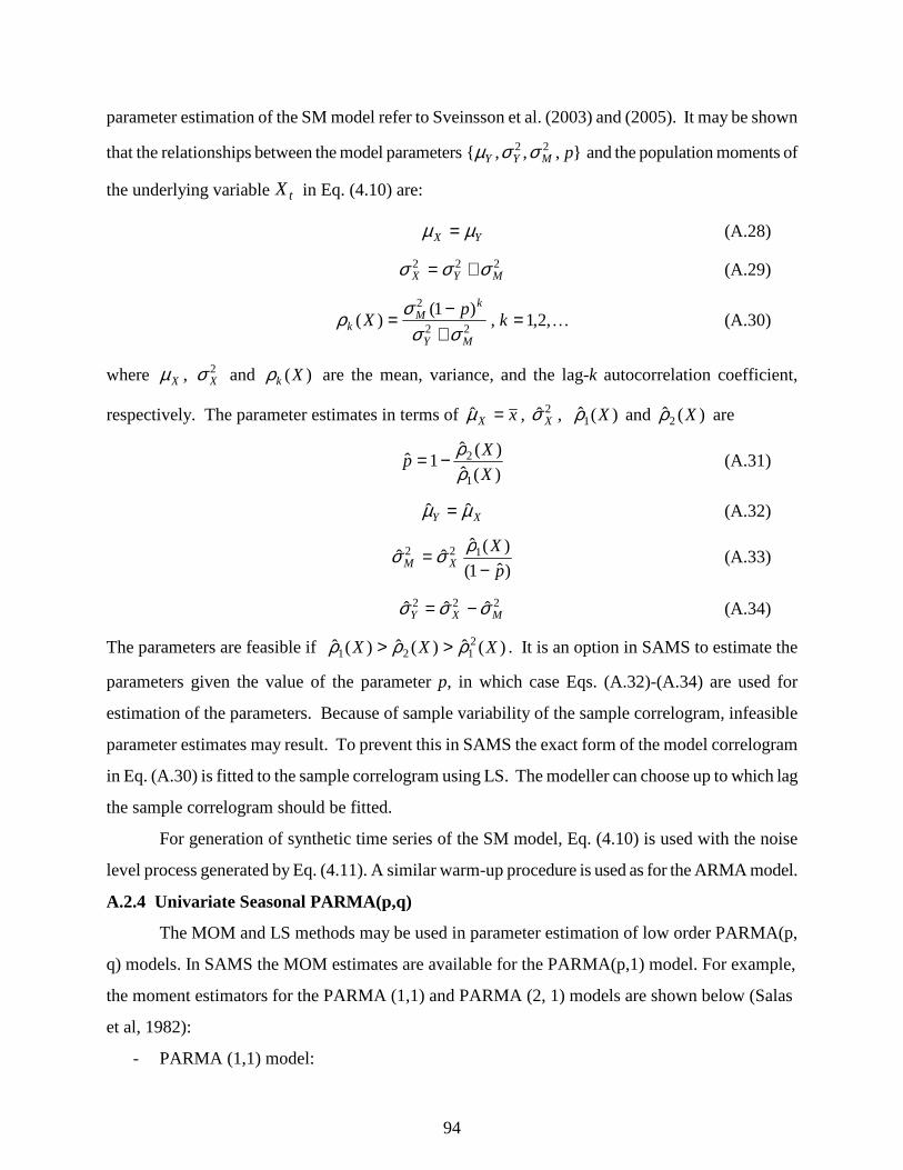
94
parameter estimation of the SM model refer to Sveinsson et al. (2003) and (2005). It may be shown
that the relationships between the model parameters },,,{ 22 pMYY σσµ and the population moments of
the underlying variableX t in Eq. (4.10) are:
YX µµ = (A.28)
222MYX σσσ += (A.29)
K,2,1,)1(
)(22
2
=+−= k
pX
MY
kM
k σσσρ (A.30)
where Xµ , 2Xσ and )(Xkρ are the mean, variance, and the lag-k autocorrelation coefficient,
respectively. The parameter estimates in terms of xX =µ , 2ˆ Xσ , )(ˆ1 Xρ and )(ˆ2 Xρ are
)(ˆ)(ˆ
1ˆ1
2
X
Xp
ρρ−= (A.31)
XY µµ ˆˆ = (A.32)
)ˆ1(
)(ˆˆˆ 122
p
XXM −
= ρσσ (A.33)
222 ˆˆˆ MXY σσσ −= (A.34)
The parameters are feasible if )(ˆ)(ˆ)(ˆ 2121 XXX ρρρ >> . It is an option in SAMS to estimate the
parameters given the value of the parameter p, in which case Eqs. (A.32)-(A.34) are used for
estimation of the parameters. Because of sample variability of the sample correlogram, infeasible
parameter estimates may result. To prevent this in SAMS the exact form of the model correlogram
in Eq. (A.30) is fitted to the sample correlogram using LS. The modeller can choose up to which lag
the sample correlogram should be fitted.
For generation of synthetic time series of the SM model, Eq. (4.10) is used with the noise
level process generated by Eq. (4.11). A similar warm-up procedure is used as for the ARMA model.
A.2.4 Univariate Seasonal PARMA(p,q)
The MOM and LS methods may be used in parameter estimation of low order PARMA(p,
q) models. In SAMS the MOM estimates are available for the PARMA(p,1) model. For example,
the moment estimators for the PARMA (1,1) and PARMA (2, 1) models are shown below (Salas
et al, 1982):
- PARMA (1,1) model:
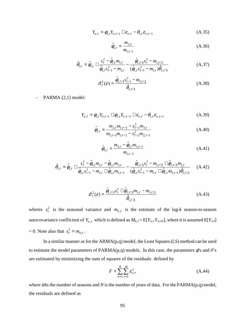
95
1,,1,1,,1, −− −+= τνττντνττν εθεφ YY (A.35)
1,1
,2,1
−=
τ
ττφ
m
m (A.36)
1,1,1
21,1
1,12
1,1
,12
1,1
,1,12
,1,1 ˆ)ˆ(
ˆ
ˆ
ˆˆˆ
+−
++
− −−
−−
−+=
ττττ
τττ
τττ
τττττ θφ
φφ
φφθ
ms
ms
ms
ms (A.37)
1,1
1,12
11,12
ˆ
ˆ)(ˆ
+
+−+ −=
τ
ττττ θ
φεσ
ms (A.38)
- PARMA (2,1) model:
1,,1,2,,21,,1, −−− −++= τνττντνττνττν εθεφφ YYY (A.39)
1,2
222,11,1
,32
22,1,2,1
−−−−
−−
−−
=ττττ
τττττφ
msmm
msmm (A.40)
2,1
1,2,1,3,2
ˆˆ
−
−−=
τ
ττττ
φφ
m
mm (A.41)
1,11,1,2,1
21,1
,11,21,12
1,1
1,1,2,12
1,1
,2,2,1,12
,1,1 ˆ)ˆˆ(
ˆˆ
ˆˆ
ˆˆˆˆ
+−−
+++
−− +−+−
−+−−−
+=ττττττ
τττττ
τττττ
τττττττ θφφ
φφφφφφ
φθmms
mms
mms
mms (A.42)
1,1
1,1,11,22
1,12
ˆ
ˆˆ)(ˆ
+
+++ −+=
τ
ττττττ θ
φφεσ
mms (A.43)
wheres 2τs is the seasonal variance and τ,km is the estimate of the lag-k season-to-season
autocovariance coefficient of τν ,Y which is defined as Mk,τ = E[Yν,τ Yν,τ-k], where it is assumed E[Yν,τ]
= 0. Note also that ττ ,02 ms = .
In a similar manner as for the ARMA(p,q) model, the Least Squares (LS) method can be used
to estimate the model parameters of PARMA(p,q) models. In this case, the parameters φ’s and θ’s
are estimated by minimizing the sum of squares of the residuals defined by
∑∑= =
=N
F1 1
2,
ν
ω
ττνε (A.44)
where ω is the number of seasons and N is the number of years of data. For the PARMA(p,q) model,
the residuals are defined as
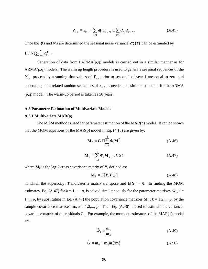
96
∑∑=
−=
− +−=q
jjj
p
iii YY
1,,
1,,,, τνττνττντν εθφε (A.45)
Once the φ’s and θ’s are determined the seasonal noise variance )(2 εστ can be estimated by
∑ =N
N1
2,)/1( ν τνε .
Generation of data from PARMA(p,q) models is carried out in a similar manner as for
ARMA(p,q) models. The warm up length procedure is used to generate seasonal sequences of the
τν ,Y process by assuming that values of τν ,Y prior to season 1 of year 1 are equal to zero and
generating uncorrelated random sequences of τνε , as needed in a similar manner as for the ARMA
(p,q) model. The warm-up period is taken as 50 years.
A.3 Parameter Estimation of Multivariate Models
A.3.1 Multivariate MAR(p)
The MOM method is used for parameter estimation of the MAR(p) model. It can be shown
that the MOM equations of the MAR(p) model in Eq. (4.13) are given by:
∑=
Φ+=p
i
Tii
10 MGM (A.46)
∑=
− ≥Φ=p
iikik k
1
1,MM (A.47)
where M k is the lag-k cross covariance matrix of Y t defined as:
][ Tkttk E −= YYM (A.48)
in which the superscript T indicates a matrix transpose and E[Y t] = 0. In finding the MOM
estimates, Eq. (A.47) for k = 1, ..., p, is solved simultaneously for the parameter matrixes iΦ , i =
1,..., p, by substituting in Eq. (A.47) the population covariance matrixes M k , k = 1,2,..., p, by the
sample covariance matrixes mk, k = 1,2,..., p. Then Eq. (A.46) is used to estimate the variance-
covariance matrix of the residuals G . For example, the moment estimators of the MAR(1) model
are:
0
11
ˆmm=Φ (A.49)
T1
1010
ˆ mmmmG −−= (A.50)
97
in which superscript -1 indicates a matrix inverse.
After estimating iΦ , i = 1,..., p, and G as indicated above, B of Eq. (4.14) can be determined
from
TBBG ˆˆˆ = (A.50)
The above matrix equation can have more than one solution. However, a unique solution can be
obtained by assuming that B is a lower triangular matrix. This solution, however, requires that G be
a positive definite matrix.
Generation of synthetic series for the MAR(p) model is carried out using Eq. (4.13) with the
spatially correlated noise generated by Eq. (4.14). The warm-up period is defined in the same way as
for the ARMA model.
A.3.2 Multivariate CARMA(p,q)
The parameter matrixes of the CARMA(p,q) in Eq. (4.15) are diagonal. Thus, as described in
section 4.3.2 the estimation of parameters of the CARMA model is done by decoupling it into
univariate ARMA models:
∑∑=
−=
− −+=q
j
kjt
kj
kt
p
i
kit
ki
kt YY
1
)()()(
1
)()()( εθεφ (A.51)
where the superscript (k) indicates the kth site and as such the parameters shown indicate the kk
diagonal element in the diagonal parameter matrixes in Eq. (4.15). The best univariate ARMA
model is identified for each site and the parameters are estimated at each site using MOM or LS
estimation methods. After having estimated the diagonal parameter matrixes pΦΦΦ ,,, 21 K and
qΘΘΘ ,,, 21 K , what remains is estimation of the noise variance-covariance matrix G. The
procedure is simple, but a necessary condition is that the CARMA(p,q) is causal. This is equivalent
to requiring each of the estimated univariate ARMA(p,q) models to be causal (often a common
requirement in estimation procedures for ARMA models). Causality implies that Y t in Eq. (4,15)
can be written out as an infinite moving average model (Brockwell and Davis, 1996):
∑∞
=−Ψ=
0jjtjt εY (A.52)
where E[Y t] = 0 and jΨ are matrixes with absolutely summable elements given by
98
∑
=−ΨΦ+Θ−=Ψ
=Ψp
iijijj
1
T
0 I
(A.53)
where 0=Ψ j for j < 0, 0=Θ j for j > q and I is the identity matrix. For the special case when p =
1 and q = 0 then jj 1Φ=Ψ , for K,2,1=j . Multiplying each side of Eq. (A.52) by its transpose and
taking expectations gives
T
00 j
jj ΨΨ=∑
∞
=GM (A.54)
Since jΨ , K,1,0=j , are diagonal matrixes the ith row and jth column element of G is
∑
∞=
=0
0
kjj
kiik
ijij M
Gψψ
(A.55)
where ijk
ijij MG ψ,, 0 are the ith row and jth column element of G, M0 and kΨ , respectively. The
elements of jΨ decay rather quickly with increasing j, thus the sum in Eq. (A.55) can usually be
truncated at a fairly low value of k. An estimate of the G matrix is obtained by replacing population statistics and parameters in Eq. (A.55) by their corresponding estimates. The above procedure for estimation of the noise variance-covariance matrix G utilizing only estimated parameter matrixes and the lag 0 covariance matrix of Y t ensures that the estimate of G is consistent with the estimates of the diagonal parameter matrixes.
Generation of synthetic series for the CARMA(p,q) model is carried out using Eq. (4.15) with
the spatially correlated noise generated in the same way as for the MAR(p) model. The warm-up
period is defined in the same way as for the ARMA model.
A.3.3 Multivariate CSM – CARMA(p,q)
The estimation of the CSM – CARMA(p,q) model is done by decoupling the model first into
its CSM and CARMA(p,q) counterparts (refer to Eq. (4.16)). The parameter of the CSM and
CARMA models are then estimated separately, where further decoupling takes place into univariate
SM models and univariate ARMA(p,q) models. This modeling option can also be used to estimate a
CSM model only or a CARMA(p,q) model only.
First it is demonstrated how the CSM part of the model is estimated. The CSM part of the
model in Eq. (4.16) has the following properties
1. The lag k covariance function of X t of the CSM model is given by
==
−+
=K,2,1
0
)1()(
kfor
kif
p kkM
MY
G
GGXM (A.56)
99
where GY and GM are the variance-covariance matrixes (lag 0 covariance matrixes) of Y and
M , respectively.
2. The sequences }{,},{},{ )()2()1( 1nttt YYY K are correlated in space at lag 0 only, and independent
in time, with ( )YG0Y ,MVN~}{ iidt .
3. The sequences }{,},{},{ )()2()1( 1niii MMM K are correlated in space only at lag zero. That is,
( )MG0M ,MVN~}{ iidi . It can be shown (Sveinsson and Salas, 2006) that a necessary
and sufficient condition for {Zt} to be stationary in the covariance is that K,, 21 NN is a
common sequence for all sites. In that case the covariance function of Zt at lag k is:
K,1,0)1()( =−= kp kk MGZM (A.57)
The condition that { }∞=1itN is a common sequence for all sites may also be supported in
practice, if the shifts in the means are thought of being caused by changes in natural
processes, such as changes in climate. In such cases it should be expected that time series of
the same hydrologic variable within a geographic region would all exhibit shifts at the same
times. Thus, in general the CSM model should not be applied for multivariate analysis of
time series if it is clear that shifts in different time series do not coincide in time. Such cases
can come up if a shift in a time series is caused by a construction of a dam or other man
made constructions, where the construction does not affect the other time series being
analyzed. Note that if M t is assumed uncorrelated in space then the condition for stationarity
that { }∞=1itN is a common sequence for all sites is not necessary any more (that option though
is not available in SAMS).
The CSM is decoupled into univariate SM models and the parameters are estimated at each site using the procedures for the SM models. If the common p is not known , then p(i) is first estimated at each site i (Sveinsson and Salas, 2006). The common p can then be estimated as a weighted
average of the )(ˆ ip s
∑=+++
=1
11
)()(1)(
1)2(
1)1(
1
ˆ1
ˆn
i
iin
pnnnn
pL
(A.58)
Given p the parameters of the univariate SM-1 models are reestimated. What remains is
estimating the non-diagonal elements of YG and MG (note the diagonal elements, i.e. the
variances, have already been estimated in the univariate models). Using Eq. (A.56) MG is
100
estimated from
p1
)(ˆ 1
−= Xm
GM (A.57)
where if necessary MG is made symmetric by replacing ijgMˆ and jigMˆ with their respective
averages. Then MG is estimated from (Eq. (A.56))
MY GXmG ˆ)(ˆ0 −= (A.58)
where as before mk(X) is the sample estimate of the lag-k covariance matrix M k(X) as defined in Eq.
(A.48).
Estimation of the CARMA part of the model in Eq. (4.16) is done by decoupling it into univariate ARMA(pi,qi), nnni ,,2,1 11 K++= models and fitting the best ARMA model for each site using the parameter estimation procedure for the multivariate CARMA model. For estimation of the variance-covariance matrix of the noise (G) of the CARMA modelled Y t, the procedures of the CARMA models are used, where each of the elements of Y t corresponding to the CSM process is looked at as being modelled by an ARMA(0,0) model. The upper left n1 × n1 part of the n × n
estimated G matrix is replaced by YG in Eq. (A.58). For generation of synthetic time series of the CSM-CARMA model, Eq. (4.16) is used
with the noise level process generated by Eq. (4.11). A similar warm-up procedure is used as for the ARMA model. A.3.4 Multivariate Seasonal MPAR (p)
The parameters of the multivariate seasonal MPAR(p) model in Eq. (4.17) are estimated by
the MOM by substituting the sample moments into the moment equations in a similar manner as for
the MAR(p) model. The moment equations of the MPAR(p) model may be shown to be:
∑=
Φ+=p
i
Tii
1,,,0 ττττ MGM (A.59)
∑=
−− ≥≥−Φ=p
iiikik kandifor
1,,, 10, ττττ MM (A.60a)
∑=
−− ≥<−Φ=p
i
Tkkiik kandifor
1,,, 10, ττττ MM (A.60b)
where M k,τ is the lag-k cross covariance matrix of Yν,τ defined as:
Tkk
Tk
Tkk EE −−−− === ττντντντντ ,
T,,,,, ]}[{][ MYYYYM (A.62)
in which the superscript T indicates a matrix transpose and E[Yν,τ] = 0. In a similar manner as for
the MAR(p) model, the MOM estimates can be found by solving Eq. (A.60) for k =1,2,..., p
simultaneously for Φ ’s by substituting the population covariance matrixes τ,kM , k = 1,…,p by the
101
corresponding sample covariance matrixes. Then Eq. (A.59) is used to estimate the variance-
covariance matrix of the residuals τG .
For generation of synthetic time series similar procedures as for the MAR(p) and
PARMA(p,q) models are used. As for the MAR(p) model the generation process of the noise is
simplified by using a lower triangular matrix τB similar as in Eq. (4.14) for the MAR(p) model, i.e.
Tτττ BBG = . As for other models a warm-up period is used to remove the effects of initial
conditions of the generation process.
A.4 Parameter Estimation of Disaggregation Models
A.4.1 Valencia and Schaake Spatial Disaggregation
The model parameter matrixes A and B of the VS model in Eq. (4.18) can be estimated by
using MOM (Valencia and Schaake, 1973):
)()( 100 XMYXMA −= (A.63)
100 )()( −−= AXMAYMBBT (A.64)
where TBBG = is the noise variance-covariance matrix (B is the Cholesky decomposition of G),
and ][)( Tkk E −= νν YYYM and ][)( T
kk E −= νν XYYXM . The VS model is not available for spatial
disaggregation of seasonal data in SAMS, since the MR model is thought to be better suited. A.4.2 Mejia and Rousselle Spatial Disaggregation
The model parameter matrixes A, B, and C of the MR model in Eq. (4.19) can be estimated
by using MOM as:
-11
10101
1010 ])()()()(][)()()()([ XYMYMXYMXMXYMYMYMYXMA TT −− −−= (A.65)
)(])()([ 1011 YMXYAMYMC −−= (A.66)
)()()( 100 YCMXYMAYMBB TT −−= (A.67)
Equations (A.65) through (A.67) can be used to obtain estimates of A, B, and C by substituting the
population covariance matrixes by their corresponding sample estimates. Lane (1981) showed that
some problems exist if one uses the above equations to estimate the parameters. Specifically, the
problem is in using )(1 XYM , since the model structure does not preserve this particular lag-1
dependence between X and Y. Lane verified this and showed that the generated moments are
affected and some key moments are not preserved. As a result, he suggested that, instead of using a
sample estimate of )(1 XYM , one should use the model )(1 XYM that would result from the model
102
structure (for further details, the reader is referred to Lane and Frevert, 1990). In the final analysis,
the suggested equation is
)()()()( 01
01*1 XYMXMXMXYM −= (A.68)
For consistency )(1 YM also needs to be adjusted
])()([)()()()( 1*1
1001
*1 XYMXYMXMYXMYMYM −+= − (A.69)
Equations (A.68) and (A.69) should be used for calculating )(1 XYM and )(1 YM , and these
calculated values should be used in Eqs. (A.65) through (A.67) for estimating the model parameters.
The reader is referred to Lane and Frevert (1990) for more in depth details about these adjustments.
A.4.3 Mejia and Rousselle Spatial Disaggregation of Seasonal Data
The model parameter matrixes τA , τB , and τC of the MR model in Eq. (4.21) can be
estimated in a similar way as for the spatial disaggregation of annual data above by using MOM.
The MOM equations are similar as for the annual MR model:
1-
,11
1,0,1,0
,11
1,0,1,0
])()()()([
])()()()([
XYMYMXYMXM
XYMYMYMYXMAT
T
ττττ
τττττ−
−
−−
−
−= (A.70)
)(])()([ 11,0,1,1 YMXYMAYMC −
−−= τττττ (A.71)
)()()( ,1,0,0 YMCXYMAYMBB TTτττττττ −−= (A.72)
where ][)( ,,,T
kk E −= τντντ YYYM and ][)( ,,,T
kk E −= τντντ XYYXM . Since the model structure of Eq.
(4.21) does not preserve the dependence structure between τν ,X and 1, −τνY for any season, same
type of adjustment procedures as for the annual MR model have to be applied for each season for
estimation of )(,1 YM τ and )(,1 XYM τ . Thus for each season the following corrected model
covariances are used:
)()()()( 1,01
1,0,1*,1 XYMXMXMXYM −
−−= ττττ (A.73)
])()([)()()()( ,1*,1
1,0,0,1
*,1 XYMXYMXMYXMYMYM ττττττ −+= − (A.74)
The above corrected model covariances need to be substituted into the MOM equations, and then the
estimates of A, B, and C are obtained by substituting the population covariance matrixes in the
MOM equations by their corresponding sample estimates.
A.4.4 Lane Temporal Disaggregation
The model parameter matrixesτA , τB , and τC of the temporal Lane model in Eq. (4.22) can
103
be estimated by using the MOM as (Lane and Frevert, 1990). To avoid confusion we have X denote
the annual flows at the N stations and Y the seasonal flows at the same stations.
1-
,11
1,0,10
,11
1,0,1,0
])()()()([
])()()()([
XYMYMXYMXM
XYMYMYMYXMAT
T
τττ
τττττ−
−
−−
−
−= (A.75)
)(])()([ 11,0,1,1 YMXYMAYMC −
−−= τττττ (A.76)
)()()( ,1,0,0 YMCXYMAYMBB TTτττττττ −−= (A.77)
where ][)( Tkk E −= νν XXXM , ][)( ,,,
Tkk E −= τντντ YYYM , ][)( ,,
Tkk E −= τνντ YXXYM and
][)( ,,T
kk E −= ντντ XYYXM . Since the model structure of Eq. (4.22) does preserve the dependence
structure between νX and 1, −τνY (i.e. )(,1 XYM τ ) for all seasons except the first one, adjustment
procedures as for the MR models need only to be applied for the first season in estimation of
)(,1 YM τ and )(,1 XYM τ . Thus only for the first season need the following corrected model
covariances to be used:
)()()()( 1,01
01*,1 XYMXMXMXYM −
−= ττ (A.78)
])()([)()()()( ,1*,1
10,0,1
*,1 XYMXYMXMYXMYMYM τττττ −+= − (A.79)
The MOM parameter matrixes are then estimated by substituting the population moments by their
corresponding sample estimates.
A.4.5 Grygier and Stedinger Temporal Disaggregation
The parameter matrixes of the contemporaneous Grygier and Stedinger disaggregation model
in Eq. (4.23) are diagonal. Similar as for other contemporaneous models the parameters of the
diagonal τA , τC , and τD matrixes are estimated by decoupling the model into univariate models for
each station and each season and estimating the parameters using the Least Squares method (LS).
What remains is estimation of Tτττ BBG = , the variance-covariance matrix of the noise for each
season. The procedure for estimating the noise variance-covariance matrixes is rigorous, and in the
case when adjustments need to be made to τG to make it positive definite, then these adjustments
are accounted for in the estimated τG for the following seasons. For detailed information on the
estimation of parameters refer to Grygier and Stedinger (1990). In the following equations we use
that the transpose of a diagonal matrix is the matrix itself. To avoid confusion we have X denote the
annual flows at the N stations and Y the seasonal flows at the same stations. For all seasons below
104
the population covariance matrixes )(0 XM and )(,0 YM τ are estimated by the sample covariance
matrixes )(0 Xm )(,0 Ym τ .
Season τ = 1:
)()( 011,0 XMAYXM = (A.80)
1011,011 )()( AXMAYMBB −=T (A.81)
Season τ = 2: Let
)()( 1,012,1 YMWYM =Λ (A.82)
)()( 1,012,0 YXMWXM =Λ (A.83)
11,012,0 )()( WYMWM =Λ (A.84)
)()()( 2,02022,0 XMDXMAYXM Λ+= (A.85)
then
22,0222,02
22,022022,022
)()(
)()()(
DXMAAXMD
DMDAXMAYMBB
Λ−Λ−
Λ−−=T
T
(A.86)
Season τ > 2: Let
11,011,011,1,0 )()()()( −−−−−− Λ+Λ+Λ=Λ τττττττ DMAXMCYMYM (A.87)
)()()( ,01,01,1 YMYMWYM Λ+=Λ −− ττττ (A.88)
)()()( 1,011,0,0 YXMWXMXM −−− +Λ=Λ ττττ (A.89)
)()(
)()()(
,011,0
11,011,0,0
YMWWYM
WYMWMM
Λ+Λ+
+Λ=Λ
−−
−−−−
Tττττ
τττττ (A.90)
)()()()( 1,0,001,0 YXMCXMDXMAYXM −− +Λ+= ττττττ (A.91)
then
ττττττ
ττττττ
ττττττ
τττττττττττ
CYXMAAYXMC
DYMCCYMD
DXMAAXMD
DMDCYMCAXMAYMBB
)()(
)()(
)()(
)()()()(
1,01,0
,1,1
,0,0
,01,00,0
T
T
T
T
−−
−
−−
Λ−Λ−
Λ−Λ−
Λ−−−=
(A.92)
If adjustments are needed for any season to make Tτττ BBG = positive definite then the following
105
adjusted estimate is used for )(1,0 YM −τ for the next season:
1111,0*
1,0ˆˆˆ)()( −−−−− −+= τττττ GBBYmYm T (A.93)
in Eqs. (A.82), (A.88), (A.90) and (A.92).
A.5 Unequal Record Lengths
The models that can deal with unequal record lengths are listed in section 4.5. When
working with different length records difficulties can arise in the use of multivariate procedures that
require the records to be of same lengths. There are several options to overcome this difficulty, the
traditional ones being to either extend the shorter records or to work with the common period of the
records. Record extension is usually the way to go, but can be a tedious task that has to be done with
a special care. Correctly done, record extension will account for changes in the mean, variance, and
autocorrelation over time. If record extension is considered to large of a task, then decisions need to
be taken whether only to use the common period of records (sometimes referred to as complete-case
methods) or to use all available data (sometimes referred to as available case methods). Using only
the common period of record has the advantages of being simple and that univariate statistics across
records can be compared since they are estimated from a common sample base. The disadvantages
stem from potential loss of information in discarding the uncommon sample base. The advantage of
using all available data is simply that all available information is being used, while the disadvantages
are that the sample base changes for variable to variable yielding problems in comparability of
statistics across variables.
The approach used in SAMS is the one of using all available data in such a way that the
overall mean and the variance of each record will be preserved. To further visualize what happens in
such an approach, the figure below shows the case of two different length records xt and yt:
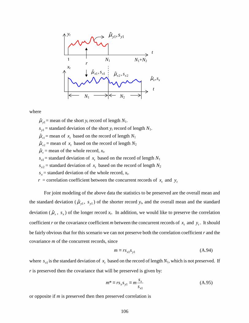
106
where
1ˆ yµ = mean of the short yt record of length N1.
1ys = standard deviation of the short yt record of length N1.
1ˆ xµ = mean of tx based on the record of length N1
2ˆ xµ = mean of tx based on the record of length N2
xµ = mean of the whole record, xt.
1xs = standard deviation of tx based on the record of length N1
2xs = standard deviation of tx based on the record of length N2
xs = standard deviation of the whole record, xt.
r = correlation coefficient between the concurrent records of tx and ty
For joint modeling of the above data the statistics to be preserved are the overall mean and
the standard deviation ( 1ˆ yµ , 1ys ) of the shorter record yt, and the overall mean and the standard
deviation ( xµ , xs ) of the longer record xt. In addition, we would like to preserve the correlation
coefficient r or the covariance coefficient m between the concurrent records of tx and ty . It should
be fairly obvious that for this scenario we can not preserve both the correlation coefficient r and the
covariance m of the concurrent records, since
11 yx srsm = (A.94)
where 1xs is the standard deviation of tx based on the record of length N1, which is not preserved. If
r is preserved then the covariance that will be preserved is given by:
1
1*x
xyx s
smsrsm == (A.95)
or opposite if m is preserved then then preserved correlation is
yt
xt
t
t
N1 N2
1 N1 N1+N2
11,ˆ yy sµ
r
22,ˆ xx sµ 11,ˆ xx sµ
xx s,µ
107
x
x
yx s
sr
ss
mr 1
1
* == (A.96)
As stated above the modeling approach is designed to preserve the long term mean and
variances of each site being modeled whether or not the different sites have equal record lengths. As
a consequence the actual historical ratio of mean flows or variances of flows between two sites is not
necessarily preserved. That is the physically consistent relationship between the two sites of the ratio
of mean flows and standard deviations is
1111 ˆˆ,ˆˆ yxyx σσµµ
while the preserved relationship will be
11 ˆˆ,ˆˆ yxyx σσµµ
Thus if there are differences in the mean and the variances of the series xt between the two flow
periods N1 and N2, then there will be some distortion in the ratio of the flows and the ratio of the
variability of the flows at the two sites from what is expected.
A.5.1 Sample Covariance Matrixes
Adjusted procedures are used in estimation of a covariance matrix for a group of sites with
unequal record lengths. These covariance matrixes are then used in the parameter estimation
procedures of the models presented in this appendix. The goal is to use a covariance estimator that
utilizes the best information from the data available, such that the overall variances at each site are
preserved and the correlation or covariance between concurrent records at any two sites is preserved.
Correlation Preserved
When the correlation coefficients are to be preserved and adjusted covariance according to
Eq. (A.95) then the lag zero variance-covariance matrix of the mean subtracted data set X
representing sites with different record lengths is estimated from
TXX vXrvXm )()( 00 = (A.97)
where Xv is a diagonal matrix with the ith diagonal value being the estimated variance from the full
record at site i, and )(0 Xr is the estimated correlation matrix with the ith row, jth column element
being estimated as the correlation coefficient computed from the concurrent record at sites i and j.
Thus the estimated covariance matrix represents the at-site variances as we wish them to be
preserved, and the corresponding covariances needed to preserve the correlation coefficient of the
concurrent record between any two sites (refer to Eg. (A.95)). If there is a need to estimate lagged
108
covariance’s, then the corresponding lagged correlation matrix is used. I.e.
Tkkttk Cov XX vXrvXXXm )(),()( == − (A.97)
gives an estimate of the lag-k variance-covariance matrix of X. The covariance matrix between two
different data arrays such as X and Y is denoted by )(XYmk as before.
Covariance Preserved
When the covariance is to be preserved and adjusted correlation according to Eq. (A.96) then
each element of the lag-k covariance matrix between X and Y, )(XYmk , is estimated as the
covariance coefficient computed from the concurrent records of the corresponding sites as for the
correlation matrix above.
A.6 Residual Variance-Covariance Non-Positive Definite
It can happen that the matrix G = BBT is not positive definite. Especially when using
different record lengths it is more likely that variance-covariance matrixes are not positive definite,
and thus adjustments are needed to make the matrixes positive definite. In the temporal
disaggregation models by Lane, and by Grygier and Stedinger, as well as in the spatial disaggregation
of seasonal data using the MR model (a condensed model), the estimated variance-covariance noise
matrix of the previous season is used for estimation of the parameters of the current season. As such,
frequent corrections to make matrixes positive definite can have an accumulated effect. To minimize
the effects of such corrections on extreme quantiles, decomposition routines that only alter the off-
diagonal values to make variance-covariance matrixes positive definite should be preferred. Thus
the variance coefficients on the diagonal are not affected, and as such extreme quantiles are more
likely to be reproduced. For the above disaggregation models and for the annual CSM-CARMA,
decomposition routines are used were off-diagonal values are reduced to make variance-covariance
matrixes positive definite. The result should be that the variance of the data will be preserved while
the covariance between two different records may be preserved in a reduced form.
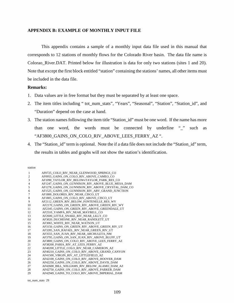
109
APPENDIX B: EXAMPLE OF MONTHLY INPUT FILE
This appendix contains a sample of a monthly input data file used in this manual that
corresponds to 12 stations of monthly flows for the Colorado River basin. The data file name is
Colorao_River.DAT. Printed below for illustration is data for only two stations (sites 1 and 20).
Note that except the first block entitled “station” containing the stations’ names, all other items must
be included in the data file.
Remarks:
1. Data values are in free format but they must be separated by at least one space.
2. The item titles including “ tot_num_stats”, “Years”, “Seasonal”, “Station”, “Station_id”, and
“Duration” depend on the case at hand.
3. The station names following the item title “Station_id” must be one word. If the name has more
than one word, the words must be connected by underline “_” such as
“AF3800_GAINS_ON_COLO_RIV_ABOVE_LEES_FERRY_AZ “.
4. The “Station_id” term is optional. Note the if a data file does not include the “Station_id” term,
the results in tables and graphs will not show the station’s identification.
station
1 AF0725_COLO_RIV_NEAR_GLENWOOD_SPRINGS_CO 2 AF0955_GAINS_ON_COLO_RIV_ABOVE_CAMEO_CO 3 AF1090_TAYLOR_RIV_BELOWvTAYLOR_PARK_RES_CO 4 AF1247_GAINS_ON_GUNNISON_RIV_ABOVE_BLUE_MESA_DAM 5 AF1278_GAINS_ON_GUNNISON_RIV_ABOVE_CRYSTAL_DAM_CO 6 AF1525_GAINS_ON_GUNNISON_RIV_ABV_GRAND_JUNCTION 7 AF1800_DOLORES_RIV_NEAR_CISCO_UT 8 AF1805_GAINS_ON_COLO_RIV_ABOVE_CISCO_UT 9 AF2112_GREEN_RIV_BELOW_FONTENELLE_RES_WY 10 AF2170_GAINS_ON_GREEN_RIV_ABOVE_GREEN_RIV_WY 11 AF2345_GAINS_ON_GREEN_RIV_ABOVE_GREENDALE_UT 12 AF2510_YAMPA_RIV_NEAR_MAYBELL_CO 13 AF2600_LITTLE_SNAKE_RIV_NEAR_LILLY_CO 14 AF3020_DUCHESNE_RIV_NEAR_RANDLETT_UT 15 AF3065_WHITE_RIV_NEAR_WATSON_UT 16 AF3150_GAINS_ON_GREEN_RIV_ABOVE_GREEN_RIV_UT 17 AF3285_SAN_RAFAEL_RIV_NEAR_GREEN_RIV_UT 18 AF3555_SAN_JUAN_RIV_NEAR_ARCHULETA_NM 19 AF3795_GAINS_ON_SAN_JUAN_RIV_ABOVE_BLUFF_UT 20 AF3800_GAINS_ON_COLO_RIV_ABOVE_LEES_FERRY_AZ 21 AF38200_PARIA_RIV_AT_LEES_FERRY_AZ 22 AF40200_LITTLE_COLO_RIV_NEAR_CAMERON_AZ 23 AF40210_GAINS_ON_COLO_RIV_ABOVE_GRAND_CANYON 24 AF41500_VIRGIN_RIV_AT_LITTLEFIELD_AZ 25 AF42100_GAINS_ON_COLO_RIV_ABOVE_HOOVER_DAM 26 AF42250_GAINS_ON_COLO_RIV_ABOVE_DAVIS_DAM 27 AF42600_BILL_WILLIAMS_RIV_BELOW_ALAMO_DAM_AZ 28 AF42750_GAINS_ON_COLO_RIV_ABOVE_PARKER_DAM 29 AF42949_GAINS_TO_COLO_RIV_ABOVE_IMPERIAL_DAM tot_num_stats 29
110
Years 98 Seasonal 12 Station 1 Station_id AF0725_COLO_RIV_NEAR_GLENWOOD_SPRINGS_CO Duration 1906 2003 66982 60131 37105 37525 38047 64812 166869 603358 809692 417092 193160 210126 108379 64733 49279 42194 50071 96240 196106 433066 1001772 718018 229194 116369 92511 59764 46132 52790 40479 62629 127924 244207 528043 237460 144038 69132 54734 46300 41728 47445 36981 53003 94156 365065 1492179 564560 199280 154107 95330 66070 47527 51775 40592 114650 192236 432027 495871 168640 103566 91501 61615 53782 40929 43131 41643 57967 107070 505588 720399 336010 140938 83611 88882 54486 40166 47237 43409 49562 84179 469364 1164973 617765 218221 108734 92922 53868 45820 45295 37443 43405 178781 452171 454694 223095 111851 88371 89738 63309 41991 45102 41898 62247 154771 770934 1132594 382642 186215 112069 101672 58314 38006 38568 37156 45815 136351 286563 584541 309362 109559 67986 71183 48013 42722 44486 39515 76730 142655 457586 730234 332998 197641 113043 96695 62460 48365 42783 40979 48255 172487 422734 1203686 620232 177627 99293 74129 68945 59410 50853 49058 79078 126500 570986 1198263 356694 132773 100034 89297 68111 52079 47061 40205 63580 156749 463641 345500 178533 114824 82416 65121 60461 51737 44661 39778 47030 74993 734672 1025073 404277 178127 106418 83106 67752 50766 49619 38960 76953 103032 639542 1176384 372525 194316 125361 75505 63162 65286 50157 46971 75605 102674 472774 700102 227573 126765 88307 59235 51476 49008 46922 41132 47049 92987 516926 930901 449785 203799 109083 111254 76335 52703 52309 48601 51715 149244 497805 814116 259635 99639 66221 84166 67813 45164 45183 40804 77956 166733 419751 470355 236521 125275 110903 91396 64705 48559 45402 39001 54752 197594 601811 888322 420167 165558 72277 65037 56936 45788 43431 38914 52940 135702 711125 711514 324628 183243 99459 95601 79431 62131 58637 46871 72912 129461 852689 814608 451908 154077 96451 77619 66884 42504 47234 41334 58493 135888 594891 945700 424620 235817 162094 110901 76219 54813 51483 47105 55027 266239 386314 604498 224591 222107 104215 79936 50877 40409 36151 35177 44368 94951 273464 398147 136312 84319 62930 51738 38483 30109 28846 30518 43989 144397 551959 676203 315056 129320 65406 58090 49708 40744 41048 33527 46979 73029 287102 948901 266211 107509 74499 62904 46937 41508 36875 33898 44832 106842 363804 184163 77343 72687 46369 38938 35332 32682 32878 29818 41314 76316 208557 719505 292846 120373 71490 57312 52782 34132 35643 34364 44126 214794 767749 615416 270357 186905 87169 65957 53581 39995 34848 36284 48119 97426 443047 378819 197450 91519 73901 67429 58744 42405 39685 39156 67985 168126 549480 949532 339706 132250 120903 70947 53927 53038 50442 40776 67632 148617 608106 460937 159126 88403 57218 55562 44186 35645 35867 36514 48635 92474 378629 416734 160366 70378 67193 72396 49412 42456 36434 37404 50491 84923 559432 512594 199903 105984 69744 75150 59316 47994 42607 40608 46403 170864 396936 752737 269106 103729 54415 50846 49200 43699 44075 41715 55982 191114 377768 651523 290818 123771 68651 54803 49054 43001 36510 38245 47533 80045 333531 588604 241426 81835 45259 46438 41902 36767 37327 36204 44520 68685 362894 566544 348464 209042 79442 69914 61124 46655 42544 41288 61161 194137 303346 504444 202783 104160 68984 66305 55748 44939 33343 42147 58331 112398 549128 675361 494113 183564 92961 80476 72139 50291 48266 48303 51670 158027 622306 549095 195700 106182 61610 55019 50876 46646 44624 40869 54644 124385 412204 766021 395249 131770 68049 69377 47693 42590 40070 40408 48636 117622 277940 614303 212420 84390 62783 54475 49261 49546 39207 43699 46766 91019 449733 740876 440071 167291 77705 71298 58153 54298 49412 42677 48439 185739 666580 1075525 321526 195481 103520 64890 55042 48392 58034 44877 57621 86564 284166 739652 243074 146609 65314 50632 55257 50101 49325 39339 44595 95489 239584 188348 119991 70003 53496 60569 48668 40662 37153 34292 43084 115940 303573 370450 178407 125269 55446 45293 49645 49765 44365 37678 55256 130022 610195 559630 152713 100601 48529 42833 46291 41707 44234 41397 48877 82779 405790 1124200 800408 235575 107050 80661 67628 58387 47085 47229 55450 85473 702806 620916 153944 87635 56025 46091 49144 48527 45269 39796 46741 85664 316390 648090 207743 117050 65122 99832 70173 47771 42496 40149 81815 204044 381424 657146 217525 95350 58241 51494 48161 41683 34846 37768 48018 67935 303658 442177 151143 116820 157794 164750 83858 55792 52436 58677 62034 354442 652543 728064 406813 146639 70234 67380 63937 48655 42399 45223 56668 101600 298438 263378 118472 122212 82759 50658 49824 38421 37055 32555 37770 73059 360298 415889 206374 111718 60328 48835 47326 48363 48033 39346 43406 111474 403793 843039 509240 235520 112587 101622 70219 60033 51315 42295 64353 101860 308340 250274 134723 87730 56271 66110 52708 41946 43206 37858 61896 113125 313901 532450 273237 111763 89660 74455 63001 50627 40685 42696 49542 83307 239313 714275 248537 165277 82753 67198 57297 53505 54369 43247 48579 152516 495605 477203 285049 124469 84804
111
99534 68529 53773 51667 48101 49606 89445 646924 728044 324818 140779 107343 107520 78589 56439 56801 53591 87036 194003 412919 813367 372231 140597 115143 86357 69319 61454 54262 50520 82030 129653 371889 658216 179920 101278 111506 95102 72427 62874 54335 47527 60767 93038 471001 727002 419052 169483 81365 72362 69298 55128 56077 49782 73795 128757 665951 656219 286117 122882 73215 75893 67402 52703 54350 52119 65065 96551 303915 661220 490561 153829 80089 62314 57959 52696 51309 53891 64242 109161 345056 441495 232808 132114 84661 72467 49566 38248 36344 35485 44764 92476 195933 250533 102959 82813 54815 62417 51366 50402 72755 44631 61093 113823 364554 826560 524972 204840 79048 69504 61360 58841 42795 45328 63979 106088 424516 748100 502968 199663 90468 79310 65104 61707 67622 64083 60419 87043 405019 718865 395812 147653 74086 62018 60106 53199 48714 36199 37216 68780 180660 346432 217544 90700 71609 61005 46826 54879 46150 38059 56801 70059 324073 634782 505031 231892 114411 103772 63707 59730 54701 47185 57651 70535 295392 945138 796122 336116 135273 100277 71109 77365 41342 64913 74365 114613 759155 1029067 643457 305878 163253 120208 106556 88230 67306 67346 89336 220625 630298 695074 376223 166450 82388 92031 95390 75647 54683 63393 103571 199973 514564 795578 514640 161439 115048 115259 96403 74765 44881 40610 47496 143451 365781 365417 198847 101350 46955 70432 65920 55366 55946 47057 69184 125677 372696 534614 332562 115617 63175 56538 42217 46468 43907 41094 67963 139104 325377 374434 228274 126582 66294 55371 60754 50190 37115 39109 42310 81947 210037 451000 285667 110453 69747 82310 48297 65646 42659 39682 44481 89779 332721 555775 330371 141464 106982 46174 80357 44404 43958 38438 51028 100890 350892 373490 247464 131607 87424 56700 70794 52588 42062 37737 40482 96171 503189 757024 504042 207955 93620 75485 62401 69346 48943 38264 56740 99169 358395 417848 205294 89234 75710 64275 54843 50394 44354 34743 53475 52437 216678 763853 732973 302524 97708 89076 73459 59770 54274 54964 63698 176645 607903 733404 351918 143289 86605 81153 91386 56034 68171 49978 68594 131076 597346 1003665 423311 200850 127746 123060 89557 74956 63650 43293 66319 113531 345083 426884 350099 176237 94519 67945 73004 71197 61824 66417 81649 91448 278322 590508 402119 179053 124181 86787 56637 66008 60078 42381 56636 107827 489284 470137 228092 115595 75113 48012 59550 65627 24466 35835 51058 80246 365363 419643 209847 107744 84498 55925 44124 53872 35838 24350 48853 67452 176288 174615 87802 77376 46494 42935 71020 43158 44687 38970 50672 79137 414097 629629 336948 141320 83834 Station 20 Station_id AF3800_GAINS_ON_COLO_RIV_ABOVE_LEES_FERRY_AZ Duration 1906 2003 458528 401644 226871 244314 292534 678174 1204640 3635101 5014167 2950460 1605086 1503159 739807 503006 353312 356760 377349 789130 1465838 2702179 5967232 5103491 1920787 955414 608812 377467 268130 276192 379543 664762 1041224 1595614 2922360 1924283 1117477 598088 483627 395707 312145 378989 317458 763721 1120492 3349297 7203254 4109919 1880422 1526396 680646 489990 377548 289322 493565 1403871 1730475 3298793 3101705 1373125 866631 630999 616468 445769 345922 367374 482597 902111 951815 2924637 4124342 2353784 1016615 593647 1138005 442055 353040 346040 327040 538145 902409 3684152 6151097 3206236 1362372 631542 636272 533065 305040 354040 314035 523340 1829661 3270774 3144985 1984476 874869 701626 670353 538369 329845 369540 401135 876055 1593814 4685650 6296013 3116692 1405438 783864 964928 527355 334330 304135 397335 525840 1483873 2427137 3642473 2147795 853538 528870 557984 411050 343247 393997 424368 1391402 1802736 3736188 4752150 2633062 1931864 809499 1402793 495715 369118 260296 351858 506891 1545288 3763312 7772051 4940893 1618993 822053 510346 448052 402771 356292 373570 655997 901047 2760607 5393082 2288860 968227 691873 569910 496385 410089 287188 316951 653288 1414719 3231444 2597757 1537305 904498 531938 377402 404787 394092 406940 601645 685472 983984 5917499 6993901 3165233 1376497 620527 534995 596367 404572 414071 456636 943675 930238 4180109 8467230 2849389 1972571 953215 488368 417789 453490 351437 438928 907266 1185878 4699578 5761054 2159890 1148518 657391 336581 400845 399832 375213 340452 449461 1316359 3835398 5077612 3053685 1744686 1013539 747521 646295 423825 312563 506890 508913 1665561 3264099 3780821 1672023 720755 389827 388361 392567 275418 262125 403157 607575 1382195 2536635 2860901 2086524 1040652 1174710 1020530 608566 447131 359577 353544 643799 1634988 3546065 4075706 1998872 966236 459006 461696 334894 379348 337439 388832 605741 1269471 4135924 4064755 3135304 1321496 2116962 979882 739253 444153 469629 463036 754898 1025978 4580808 4271762 2241461 1048280 558717 625418 570090 344257 331823 346061 923749 1698112 4276261 5414640 2744488 2389754 1742400 964743 560310 437244 298790 485407 575246 1792671 2168481 3724824 1693721 1891015 691053 587559 423714 288560 263662 366639 429833 597640 1387684 2042727 1147598 671677 424426 536283 353322 252643 272930 557282 673831 1676128 4286246 4193514 2684941 1364498 693906 367644 378380 272887 273376 255953 501362 515700 1604249 4680018 1898287 818373 563832 440664 297779 333907 308075 303395 349072 557263 1480351 1018245 721126 532811 284828 212899 181355 228772 254933 274011 339574 685733 1585305 4708552 2255472 959192 594224 387726 319435 266192 264047 318400 459898 1400149 4032422 3360120 1709054 1262461 705479
112
376632 443083 317128 200331 414259 700570 1559558 3833665 2958383 1923464 838115 596566 505920 384592 390633 325637 354575 794138 1659082 3599128 5324845 2503358 1027381 1050775 618499 479804 411097 348487 300377 809304 1228538 2865278 2250280 1104801 629626 671962 358134 312958 284314 261837 301174 439068 735512 2442459 2212812 984226 522322 525463 731809 410102 364873 355941 430079 675567 1127132 5323093 4598652 2428433 1190375 683285 1813960 913232 576929 404450 395910 660985 2902862 3500486 4834784 2074078 938573 412011 358326 373655 369016 345094 344573 533607 1624861 2446508 3294191 2132619 1188466 613563 386115 442637 379167 284953 344393 515043 1060878 3622415 4760167 2526378 857685 332678 378318 378988 307526 330444 359434 430301 790464 3150282 3358331 2468347 1465735 494543 538329 434400 319918 348056 313504 506085 1141098 1970811 2755500 1432801 852859 449365 430011 472765 422598 265000 353367 656705 844051 3600478 3790869 2726585 1575216 778634 830411 577524 440646 375949 432004 624879 1728270 4032836 3915190 1662639 887163 372680 361999 399745 345940 326826 350930 692324 1377417 3474042 5116808 2809867 985997 420279 539733 475823 363538 346883 394729 631678 1270496 2239296 3782181 2027117 817606 428842 423062 355831 422695 307758 356588 416528 564533 2034805 3694508 2205007 1172271 532247 430044 451352 340253 490658 385654 435309 2329319 5569121 6201051 2317967 1255129 694186 376061 376582 374385 402474 365207 458845 554827 1285021 3910327 1662389 1032517 405366 318406 427066 342974 317925 341586 388722 666898 1753441 1396009 1255884 664718 494512 570813 355936 289658 254680 252729 590617 697977 1950795 2332135 1220313 920244 359573 225234 274490 335121 379784 279980 513692 993694 2814517 3534913 1151798 703754 298120 193813 304643 258166 295275 331116 508805 868604 2805792 6669099 4906010 2007877 1010603 756358 838468 502956 392045 536727 688965 1599996 4597690 4562509 1308184 677219 438820 333453 358554 368349 306407 313512 350118 463516 1380376 2826173 1448923 766845 316311 557316 517710 350962 289809 314720 749816 1720737 1977890 3222979 1361812 582813 328283 361418 348931 264952 244498 318919 368225 637529 1642974 2528584 956734 718990 856024 819598 547420 370764 334494 774737 545028 2532520 4119768 3849168 2550866 912852 412135 555007 448064 342970 201557 370712 575260 763590 1808387 1839152 933748 685572 735431 319363 342117 266011 267885 262479 343862 649129 2354779 2984535 1729449 915192 366401 301361 325117 363397 379725 369167 443493 1400634 3392487 5596742 3793601 1623391 877286 875445 570571 552485 455182 395360 981129 1333026 2523296 1934274 1053979 589839 357643 335665 349297 371154 289340 307306 576121 604735 1690771 3628249 2187199 951241 517396 351908 327692 238872 313145 337745 517660 639473 2123875 5021980 1742269 1468908 424710 443620 385800 320747 391523 352823 571807 1972984 3869865 3004303 2035789 892706 607745 675186 513856 383572 382737 361005 447329 615374 3630445 4189472 2096715 917019 1131553 649771 515681 407035 494028 491917 609586 1346671 2442170 4378219 2193103 898173 672638 661344 551215 479703 503247 467405 821308 823858 1927411 3758045 1164322 651283 570793 1117457 673421 453960 440638 460070 850577 1352785 4438702 5017892 2725430 995488 671589 463087 519916 440926 461515 405635 789606 941881 3337175 3326953 1524780 707333 366575 408958 509477 344922 427953 377807 626521 867004 2690100 4980524 3983484 1022959 525705 405373 448805 425556 398670 474045 549727 842291 2425697 2791610 1295121 741627 491105 442882 374018 283634 323678 293529 279558 362869 621039 948914 655405 568483 370874 324926 342911 315076 366742 305861 615011 1229315 2725495 4996726 2527981 792844 409148 347725 487162 398648 388798 359164 748474 1813403 3987890 5216554 2656609 1048268 418098 366547 408377 359686 477018 610450 643393 1423153 4334181 5335616 2224502 714267 608819 415724 481358 427048 392521 321594 365405 625969 1207244 2350327 1142295 520895 542125 645087 465497 407287 353944 322075 649796 980164 3005422 4261797 2997487 1549240 1080058 997492 726531 620587 395661 459797 896921 1130239 3529632 7749358 5119270 2123359 847309 1056364 707826 650196 436388 516388 855802 1439814 6051182 6696277 3864820 1957909 1063077 1042063 829281 644638 588807 590005 1126236 2928584 4877643 4709583 2281036 1097301 738505 914200 748568 638841 549620 744835 1089259 2171122 3843805 6019606 3406845 1334490 992365 1144081 999075 730182 526848 623570 948887 1875380 3672651 3171561 1549328 1035658 655526 490099 630954 431240 358635 413160 716818 1045200 2042327 2757869 1464669 866077 579061 478381 379938 344918 331736 369328 824829 1195159 1738912 1989335 1218965 819605 458147 378394 412665 300616 283874 286727 406718 623336 1272203 2650122 1431174 734448 546716 584293 452232 300982 302663 387347 488399 805069 2142072 3397023 1576149 966693 798055 366329 571913 355320 331233 423080 597821 1077164 2233709 2128362 1358845 893001 639570 390254 461410 317306 422016 406299 850921 1306387 4392963 5018064 2568377 1197118 773740 565586 473521 405719 394861 356573 667133 796880 2280260 2463400 1063026 680931 529090 535822 461242 392859 365597 451478 838692 711196 2276743 6260631 5275349 1721807 746118 665334 549699 472341 432199 506944 548217 1093148 3310201 3633660 2037048 780273 539180 574916 626952 506313 501689 446694 1051532 1459934 4542370 6138492 2439388 1511481 1225995 1045442 719272 555801 522285 476725 751272 1315036 3592304 3606179 2583291 1300234 734395 705799 758134 500151 486391 427290 670363 798775 2578717 4445246 2538308 1606115 1074032 597603 512581 410215 441605 431047 519651 1116217 2559824 2296158 1076228 636522 537722 465751 458174 402471 304030 321668 583675 901810 2742548 2294801 1166622 824135 482174 370904 383981 334526 301419 255292 374686 584548 811697 1124148 727763 438371 483371 361480 428525 297771 283654 279225 499211 644975 2002318 2954098 1215702 622129 674693
113
APPENDIX C: EXAMPLE OF ANNUAL INPUT FILE
This appendix contains a sample of an annual input data file used by SAMS corresponding to
98 stations of annual flows for the Colorado River basin. Printed below for illustration are data for
only two stations (sites 1 and 20).
tot_num_stats 12 Years 98 Annual Station 1 Station_id AF0725_COLO_RIV_NEAR_GLENWOOD_SPRINGS_CO 705000 3105000 1705000 3150000 1900000 2193000 2987000 1828000 3084000 1814000 2297000 3036000 2867000 1702000 2832000 2978000 2095000 2598000 2280000 1891000 2690000 2469000 2915000 2833000 2204000 1337000 2106000 2027000 1118000 1700000 2401000 1561000 2575000 1859000 1442000 1821000 2060000 1989000 1640000 1878000 1701000
114
2408000 2044000 2190000 1658000 2250000 2873000 1894000 1056000 1414000 1884000 3021000 2063000 1716000 1996000 1501000 2836000 1311000 1474000 2491000 1329000 1738000 1854000 1944000 2409000 2488000 1956000 2354000 2310000 2154000 1688000 1056000 2456000 2414000 2227000 1273000 2184000 2965000 3445000 2710000 2786000 1641000 1908000 1558000 1494000 1880000 1596000 2462000 1597000 2468000 2495000 2899000 1967000 2088000 1855000 1552000 893000
115
1976000 Station 20 Station_id AF3800_GAINS_ON_COLO_RIV_ABOVE_LEES_FERRY_AZ Duration 1906 2003
18210000 21230000 11770000 21840000 14740000 15130000 19080000 14470000 21070000 14140000 19190000 23850000 15750000 12950000 21930000 22700000 18670000 18340000 14640000 13410000 16110000 18550000 17580000 21410000 15280000 8632000 17550000 12130000 6628000 12280000 14490000 14160000 17920000 11720000 9380000 18320000 19430000 13620000 15510000 13910000 11060000 15920000 15880000 16660000 13320000 12490000 20900000 11200000 8368000 9795000 11510000 20160000
116
16900000 9233000 11970000 9248000 17770000 9259000 10800000 18870000 11620000 11810000 13510000 14850000 15340000 15100000 12380000 19200000 13290000 16770000 11290000 5525000 14950000 17870000 17510000 8793000 16720000 24600000 25300000 21450000 22450000 16930000 11800000 10150000 9327000 12200000 10980000 18100000 10680000 20040000 14570000 21030000 17200000 16590000 11140000 10950000 6191000 10260000
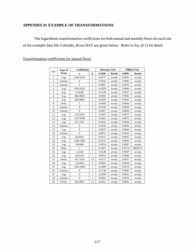
117
APPENDIX D: EXAMPLE OF TRANSFORMATIONS
The logarithmic transformation coefficients for both annual and monthly flows for each site
of the example data file Colorado_River.DAT are given below. Refer to Eq. (4.1) for detail.
Transformation coefficients for annual flows
Coefficients Skewness Test Filliben Test
Site Type of Trans a b 0.3928 Result 0.9891 Result
1 Log 2324.1916 1 -0.0777 accept 0.9942 accept
2 Gamma 0 1 0.0656 accept 0.9983 accept
3 Gamma 0 1 0.0801 accept 0.9943 accept
4 Log 4334.4335 1 -0.0259 accept 0.9964 accept
5 Log 23.4228 1 -0.1336 accept 0.9927 accept
6 Log 884.0838 1 0.0920 accept 0.9946 accept
7 Log 636.9696 1 0.0329 accept 0.9943 accept
8 None 1 1 -0.0456 accept 0.9944 accept
9 Gamma 0 1 0.0338 accept 0.9958 accept
10 Gamma 0 1 0.0067 accept 0.9958 accept
11 Log 252.0259 1 -0.0475 accept 0.9977 accept
12 Log 1197.9786 1 0.0283 accept 0.9973 accept
13 Log 677.2791 1 0.0554 accept 0.9958 accept
14 Gamma 0 1 0.0356 accept 0.9964 accept
15 Log 0 1 -0.0376 accept 0.9944 accept
16 Gamma 0 1 0.0072 accept 0.9932 accept
17 Log 66.6643 1 0.0375 accept 0.9951 accept
18 Log 2540.7005 1 0.0114 accept 0.9949 accept
19 Log 194.098 1 -0.0514 accept 0.9967 accept
20 None 1 1 0.1947 accept 0.9774 REJECT
21 Log -3.2543 1 -0.0148 accept 0.9967 accept
22 Log 46.0528 1 0.0554 accept 0.9948 accept
23 Power 457.3136 1.9 -0.0117 accept 0.9957 accept
24 Log -55.4413 1 0.0024 accept 0.9958 accept
25 Log 1062.5804 1 -0.0409 accept 0.9974 accept
26 Gamma 0 1 -0.1730 accept 0.9905 accept
27 Log 0 1 -0.2582 accept 0.9921 accept
28 Gamma 0 1 0.0282 accept 0.9974 accept
29 Power 683.0857 1.3 0.0253 accept 0.9966 accept
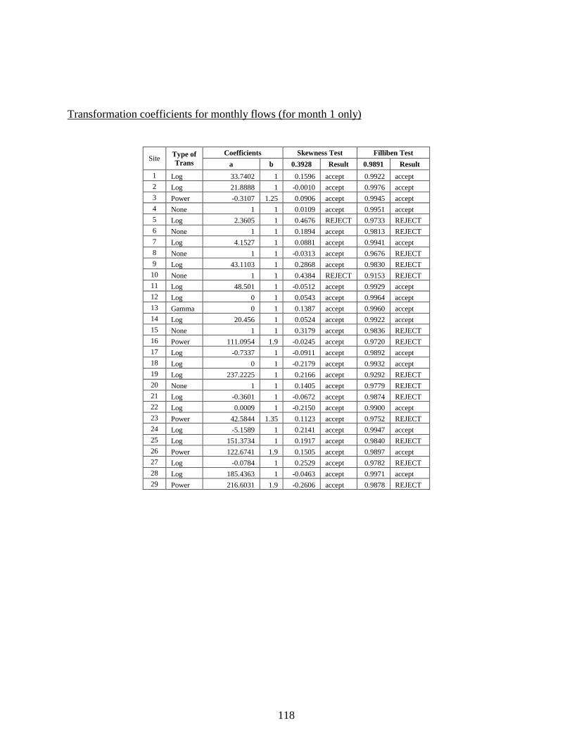
118
Transformation coefficients for monthly flows (for month 1 only)
Coefficients Skewness Test Filliben Test Site
Type of Trans a b 0.3928 Result 0.9891 Result
1 Log 33.7402 1 0.1596 accept 0.9922 accept 2 Log 21.8888 1 -0.0010 accept 0.9976 accept 3 Power -0.3107 1.25 0.0906 accept 0.9945 accept 4 None 1 1 0.0109 accept 0.9951 accept 5 Log 2.3605 1 0.4676 REJECT 0.9733 REJECT 6 None 1 1 0.1894 accept 0.9813 REJECT 7 Log 4.1527 1 0.0881 accept 0.9941 accept 8 None 1 1 -0.0313 accept 0.9676 REJECT 9 Log 43.1103 1 0.2868 accept 0.9830 REJECT 10 None 1 1 0.4384 REJECT 0.9153 REJECT 11 Log 48.501 1 -0.0512 accept 0.9929 accept 12 Log 0 1 0.0543 accept 0.9964 accept 13 Gamma 0 1 0.1387 accept 0.9960 accept 14 Log 20.456 1 0.0524 accept 0.9922 accept 15 None 1 1 0.3179 accept 0.9836 REJECT 16 Power 111.0954 1.9 -0.0245 accept 0.9720 REJECT 17 Log -0.7337 1 -0.0911 accept 0.9892 accept 18 Log 0 1 -0.2179 accept 0.9932 accept 19 Log 237.2225 1 0.2166 accept 0.9292 REJECT 20 None 1 1 0.1405 accept 0.9779 REJECT 21 Log -0.3601 1 -0.0672 accept 0.9874 REJECT 22 Log 0.0009 1 -0.2150 accept 0.9900 accept 23 Power 42.5844 1.35 0.1123 accept 0.9752 REJECT 24 Log -5.1589 1 0.2141 accept 0.9947 accept 25 Log 151.3734 1 0.1917 accept 0.9840 REJECT 26 Power 122.6741 1.9 0.1505 accept 0.9897 accept 27 Log -0.0784 1 0.2529 accept 0.9782 REJECT 28 Log 185.4363 1 -0.0463 accept 0.9971 accept 29 Power 216.6031 1.9 -0.2606 accept 0.9878 REJECT