STOCHASTIC ANALYSIS OF EGRESSSIMULATIONS

JULLIEN Quentin and LARDET Paul1 Université Paris-Est, Centre Scientifique et Technique du Bâtiment (CSTB), Safety,

Structures & Fire Department, Expertise, Regulatory Advice & Research Divisionquentin.jullien@cstb.fr

2 Université Paris-Est, Centre Scientifique et Technique du Bâtiment (CSTB), Safety,Structures & Fire Department, Expertise, Regulatory Advice & Research Division

lardet.paul@cstb.fr

Abstract. The use of egress simulation models in performance-basedanalysis relies on the confidence in the input and output data. Thesedata strongly depend on a large number of parameters. The study pre-sented here focuses on the statistical aspects of these data, especiallythe population behavioral parameters which are the most likely to bescattered. The study proposes a method to analyze the statistical as-pects of an egress simulation model. The method is based on statisticalestimations of the distribution quantiles of the output parameters andcan be applied to stochastic simulations results. It provides quantitativeinformations on the key output parameters dispersion, such as RequiredSafe Egress Time (RSET). It also gives a justification to the requirednumber of simulations and input parameters precision to ensure a rel-evant output precision level. It gives access to quantitative criteria tocompare experimental and numerical data. This method will be appliedto analyze case studies simulated with BuildingExodus.

1. INTRODUCTIONThe practice of the egress engineering relies on numerical models. Their mainpurpose is to determine the time taken by last occupant to evacuate a buildingeither in normal or accidental situation. This time is called Required Safe EgressTime (RSET) all along the present document. The various human behaviorphenomena occurring during an evacuation are not deterministic. Indeed, theintrinsic behavior of a person, for example its response time before movement,can be scattered from case to case. As a result, the egress phenomena is scatteredin itself, and a given starting situation can lead to many different evacuationsprocess.

Some previous work has already dealt with this scattered aspect of the phe-nomena. For example, Tavares and Ronchi [2] propose a method to evaluate andtake into account uncertainties in egress engineering studies. Cuesta, Ronchiand Gwynne study some school building evacuation test data [1]. They then usethose data as inputs for numerical simulations of the egress process and proposea comparison method between experimental and numerical results.

Although these previous work cover the scattered aspects of one particularsituation, it is still quite difficult to encompass the whole range of possibilitiesof an egress process. The work presented here proposes a method to study thesedifferent possibilities. This method includes the scattered aspects of the humanbehavior, as well as the different usages for a given building. A stochastic ap-proach is set up for that purpose, in order to evaluate a relevant RSET value.A statistic treatment is also applied in order to take into account the randomaspects of the resulting data. Using a numerical tool is appropriate as it allowsto easily perform a large number of RSET evaluations.

The numerical tool used in this research study is BuildingExodus v6.2. It usessophisticated sub-models means to take into account interactions like occupant-occupant, occupant-fire and occupant-building. Each occupant is individuallymodeled and has its own characteristics. This is essential to the study presentedhere. BuildingExodus is also able to process the large number of simulationsneeded to conduct this study.

The statistical analysis method set up here requires some precautions. First,it is essential to identify the parameters (response time, walking speed, inter-actions between people), which may impact the outputs. The statistical distri-bution of their value is needed in order to produce relevant results. However,very few statistical informations are available from literature. Usually only aminimum, maximum and a mean values are available. Thus, only uniform distri-bution laws are used in this study. This first order hypothesis does not impactthe mathematical method, but needs further improvements.

The statistical analysis method is based on statistical estimation of the out-put parameters quantile distribution (RSET in this document). The aim of thismethod is to provide quantitative elements on statistical distribution of RSET.It gives quantitative arguments to validate the number of simulations performed,compared to the expected precision. A particular focus will be done on the RSET95th percentile.

2. STATISTICAL ANALYSIS METHOD:IMPLEMENTATION AND STATISTICAL ELEMENTSAs an example, the statistical analysis method is applied to a sample of n realiza-tions of a random variable which distribution is normal. In the following sectionsthe variable considered will be the RSET. 60 samples are randomly drawn.

A confidence interval Ip is calculated for each quantile α from the sample ofsize n = 60 by choosing a level of confidence p equal to 90%. The confidenceinterval is the interval which includes the real value of the estimated quantileswith a 90% probability. This confidence interval is calculated as follows:

Ip =

[F̃−1

(α− c

√α(1− α)

n

); F̃−1

(α+ c

√α(1− α)

n

)]with:

– F̃ the empirical distribution function,

2

– c the quantile (1− p2 ) of the normal law distribution. c is equal to 1.645 for

p = 90%.

The distribution function is said empirical as opposed to the real distributionfunction, which is generally unknown.

Figure 1 shows the random variable realizations ranked in ascending ordergenerating the empirical distribution function as well as lower and upper boundsof each percentile confidence intervals.

Figure 1. Empirical distribution function of the random variable, lower and upperbounds of the confidence interval and real distribution function

This example highlights the problems related to extreme values of a randomvariable: in some cases, the random variable will have no maximum upper value.This is the case in this simple example, but can also happen for some RSETevaluations.

In most of the cases, a maximum value exists, but the finite samples numberprevent from calculating this maximum value. A stochastic analysis can indeedonly give percentiles, which get closer to 100% when the number of sample grows.

3

In addition, a maximum RSET value can reflect very extreme scenarios where allworst case situations happen simultaneously. The value of this kind of extremecases is questionable.

Furthermore, the confidence interval width decreases when the samples num-ber increases.

Consequently, the required number of draws required by a stochastic analysisis set by:

– the order of the desired percentile,– the required precision, which imposes the size of the confidence interval.

3. HYPOTHESIS OF THE MODELThe numerical tool used in this study is BuildingExodus. However, any kind ofegress simulation could be processed by the mean of the proposed method.

BuildingExodus is based on a discretization of space by interconnected nodesof 50 cm x 50 cm. The connection model is the Moore’s model as shown onfigure 2.

Figure 2. Nodes connectivity under BuildingExodus

The test case is a 16 m square room with 4 exits distributed on each side (fig-ure 3). Each occupant occupies one complete node. Two occupants cannot coexiston the same node. The exits are 3 m of wide, and their flow rate is 2.0 occu-pant/m/s.

4

Figure 3. Test case geometry

Concerning population, some attributes are arbitrarily fixed and others are vari-able depending on test cases:

– occupants have identical leaderships (in this case 10). This parameter affectshow conflicts are resolved when two occupants want to occupy the same nodewhich is impossible. BuildingExodus applies by default a conflict resolutiontime between 0.8 s and 1.5 s to the occupants. For some test cases, theconflict resolution time is set at the average value of the interval, that is tosay 1.15 s.

– occupant’s patience is imposed to 10 s. This implies that the occupants arewilling to remain static in a queue for 10 seconds before attempting to changedirection.

– occupants are all valid,– their speed is 1.2 m/s,– the response time is set at 15 s or variable between 0 and 30 s depending

on the test case. The response time in this study is the delay before theoccupants begin to move toward the exit.

– occupants act independently of each other: if an occupant begins to movetoward the exit he will not make another occupant move before its responsetime is elapsed.

5

This document do not present the attributes specifically related to fire such as in-capacitating concentrations of toxic gases (HCl, HBr, HF, SO2, NO2, CH2CHO,…)because they have no influence on the treated cases.

Varying parameters are randomly drawn according to a uniform law betweentwo extreme values. The most advanced behavioral options are left at their de-fault values (e.g: occupants are aware of all exits). The objective of the occupantsis to reach the nearest exit from their initial position. Finally, when several simu-lations in large numbers for the same test cases are performed, they are not usedagain from one case to another. That is to say that if 100 and 1,000 achievementsare performed, the first 100 are not part of the following 1,000. The draw is com-pletely redone every time. These choices are made for simplification purposes.They are meaningless regarding to the proposed analysis method.

4. STUDY

4.1. Use of the statistical analysis method

In this reference test case, two random simulations sets are carried out. Eachsimulation takes into account a random occupant number between 1 and 1,000,randomly located in the room. The first set contains 100 simulations, the sec-ond one contains 1,000 simulations. Figures 4 and 5 show the calculated RSETdistribution functions as well as the lower and upper bounds of the confidenceintervals for 100 simulations, respectively 1,000 simulations. The selected levelof confidence is 90% (the same level of confidence is used in the rest of thedocument).

Figure 4. Distribution function for 100 simulations and lower and upper bounds ofthe confidence interval (reference test case)

6

Figure 5. Distribution function for 1,000 simulations and lower and upper bounds ofthe confidence interval (reference test case)

Note that the number of simulations is too low to reach the theoretical minimumRSET corresponding to a single occupant positioned in front of an exit. Indeed,one could expect a RSET close to 15 s in this case (RSET = response time +traveling time, minimum traveling time being 0 s).

In accordance with what has been announced above, it is observed that:

– the confidence interval width decreases when simulation number increasefrom 8.1 s on average for 100 simulations to 2.5 s on average for 1,000 sim-ulations,

– extreme percentiles have unbound confidence intervals for 100 and 1,000 sim-ulations.

Thus, it is not possible to statistically determine a maximum RSET value. Ta-ble 1 shows the confidence intervals associated with the 95th percentile for 100,200, 500, 1,000 and 5,000 simulations. This choice implies that in 95% of cases alloccupants have evacuated with a probability of 90%. The choice of the studiedpercentile order should be discussed in further studies, as it is the key parameterassociated to the building safety level. The confidence level impacts the confi-dence interval width, and must be chosen according to the required precision(see section 2).

7

Confidence interval Width of confidence intervalof the 95th percentile (s) of the 95th percentile (s)

100 simulations [76.9 ; 82.6] 5.7200 simulations [76.6 ; 80.0] 3.4500 simulations [78.0 ; 79.7] 1.71,000 simulations [78.4 ; 79.3] 0.95,000 simulations [78.1 ; 78.8] 0.7

Table 1. Confidence intervals of the 95th percentile for 100, 200, 500, 1,000 and 5,000simulations

Figure 6 shows the confidence interval width for the 95th percentile accordingto the number of simulations. There are a number of simulations for which thewidth of the confidence interval is sufficiently low to be acceptable. Moreover,beyond this number an increase of the number of simulation does not providesignificant accuracy (see table 2) while it considerably increases the computingtime. Indeed, the simulations are all performed in very short times, despite thefact that the population can vary from 1 to 1,000 occupants: the time spent toperform the simulations is proportional to the number of simulations (simula-tions are achieved in a sequentially way). So for all these reasons, 1,000 simula-tions seem to be sufficient in the case studied here.

In conclusion, the proposed statistical analysis method quantitatively evalu-ates the number of simulations that seems most relevant to carry out a study.

Figure 6. Confidence interval width vs. number of simulations

8

Decrease of the confidenceinterval width (%)

100 simulations Reference200 simulations 40500 simulations 701,000 simulations 845,000 simulations 88

Table 2. Decrease of the width of the confidence interval according to the number ofsimulations

4.2. Complementary analysis

At least three separate evacuation patterns exist according to the number ofoccupants (see figures 4 and 5) the table 3 gives the correspondence with theRSET obtained. These three patterns correspond to three density ranges ofpeople highlighting its influence on the RSET. Indeed, the density of people hasinfluence on the congestion time and the average occupants speed.

Pattern 1 Pattern 2 Pattern 3RSET (s) [22.4 ; 37.4] [37.4 ; 72.2] [72.2 ; 82.6]Occupants number [34 ; 297] [297 ; 806] [806 ; 982]Population density (person/m²) [0.1 ; 1.2] [1.2 ; 3.1] [3.1 ; 3.8]Average waiting time (s) 2.7 13.5 23.5Average speed (m/s) 0.8 0.3 0.2

Table 3. Ranges of differents patterns for 100 simulations

The figures 7 and 8 show the occupants number scattering according to RSETfor 100 and 1,000 simulations. A greater dispersion is observed for the patternn°1. In this case, the RSET is controlled by the distance from the last occupantto the exit, rather than the population density. It demonstrates the interest ofthe approach developed in this document, which provides additional elements tounderstand evacuation behaviors.

9

Figure 7. Occupants number scattering vs. RSET for 100 simulations

Figure 8. Occupants number scattering vs. RSET for 1,000 simulations

10

As there are very little simulations with the same number of occupant, it isimpossible to quantify the influence of position and conflict resolution time onthe RSET at this stage of the study. This is the topic of the next section.

5. ANALYSIS OF THE PARAMETERS’ STATISTICALINFLUENCEThis section studies the influence of some parameters on the results of the ref-erence test case for the three patterns previously identified. Table 4 shows thecharacteristics of each test case.

Parameters of the sensibility studyConflict Position of the Response Number of

resolution time (s) occupants time (s) simulationsTest case 1 [0.8 ; 1.5] Fixed 15Test case 2 1.15 Fixed 15 1000Test case 3 [0.8 ; 1.5] Random 15Test case 4 [0.8 ; 1.5] Random [0 ; 30]

Table 4. Synthesis of studied influences for the test cases n°1, 2, 3 and 4

For each case 3 sets of simulations are performed. Each of these sets takesinto account a fixed number of people, corresponding to the median RSET ofeach pattern identified above.

Table 5 shows the characteristics of these simulations.

pattern 1 pattern 2 pattern 3Reference case RSET (s) 30.5 55.8 78.3Occupants number 187 610 927Population density (person/m²) 0.7 2.4 3.6

Table 5. Simulations selected for test cases n°1, 2, 3 and 4

5.1. Test case n°1Three sets of 1,000 simulations are run, each set having a fixed occupant num-ber and occupant location. The conflict resolution time is the only random pa-rameter, and has a uniform distribution law. Figure 9, 10 and 11 present thedistribution functions as well as the lower and upper bounds of the confidenceintervals. The empirical distribution functions are clearly not uniform. Yet, onlythe conflict resolution time is scattered. It demonstrates the sophisticated inter-actions between input parameters and RSET, as a uniform random parametercan lead to complex statistical REST behavior.

11

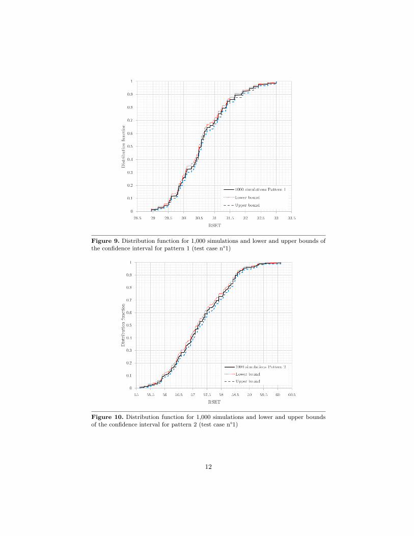
Figure 9. Distribution function for 1,000 simulations and lower and upper bounds ofthe confidence interval for pattern 1 (test case n°1)

Figure 10. Distribution function for 1,000 simulations and lower and upper boundsof the confidence interval for pattern 2 (test case n°1)

12

Figure 11. Distribution function for 1,000 simulations and lower and upper boundsof the confidence interval for pattern 3 (test case n°1)

Table 6 summarize the three simulations sets results:

– 95th percentile confidence interval (Ip95%),– width of Ip95% LIp95% (see figure 12),– the interval between the lower bound of the 5th percentile and the upper

bound of the 95th percentile Ip5%−95%,– width of Ip5%−95% LIp5%−95% (see figure 12),– the ratio between LIp5%−95% and the 50th percentile LIp5%−95%/q50%.

RSET Ip95% LIp95% Ip5%−95% LIp5%−95% LIp5%−95%/q50%

reference (s) (s) (s) (s) (%)test case

(s)S. 1 30.5 [32.1 ; 32.4] 0.3 [29.4 ; 32.4] 3.0 10.0S. 2 55.8 [58.8 ; 59.1] 0.3 [55.8 ; 59.1] 3.3 5.8S. 3 78.3 [79.2 ; 79.7] 0.5 [75.6 ; 79.7] 4.1 5.4

Table 6. Synthesis of the results obtained

13

Figure 12. Confidence intervals width for the 3 patterns of the test case n°1

There is a certain variability of the RSET even when the starting positions of theoccupants are fixed. As commented above, this variability is due to the variabilityof the conflict resolution time as well as to the effect of history produced bythe various collisions. It is coherent with the fact that LIp95% is higher for thepattern including a bigger density of people. The same phenomenon is observedfor LIp5%−95%. It is reminded that the choice of the 95th percentile and byextension the one of the 5th percentile depends on the objectives of the study.

5.2. Test case n°2

For this second test case the conflict resolution time is fixed to its average value1.15 s. This allows to separate the impact of the conflict resolution time vari-ability from the history effect. Again, 3 sets of 1,000 simulations are run, eachone with a fixed occupant number and occupant location.

In this case too, the distribution functions are not uniform despite the factthat conflict resolution time is fixed to 1.15 s. It demonstrates the strong non-linearity of the history effects. In addition, this implies that the distributionfunctions of test case 3 and 4 will not be uniform. Synthetically, table 7 presentsIp95%, LIp95%, Ip5%−95%, LIp5%−95% and LIp5%−95%/q50% for the three simula-tions and compared to those of the test case n°1. The widths of intervals areincluded in figure 13. This demonstrates the very weak influence of the conflictresolution time on the results, at least in this simple case.

14

Test S. Ip95% LIp95% Ip5%−95% LIp5%−95% LIp5%−95%/q50%case (s) (s) (s) (s) (%)

1 [32.1 ; 32.4] 0.3 [29.4 ; 32.4] 3.0 10.01 2 [58.8 ; 59.1] 0.3 [55.8 ; 59.1] 3.3 5.8

3 [79.2 ; 79.7] 0.5 [75.6 ; 79.7] 4.1 5.41 [31.0 ; 32.0] 1.0 [29.2 ; 32.0] 2.8 9.2

2 2 [58.8 ; 58.9] 0.1 [56.0 ; 58.9] 2.9 5.13 [79.3 ; 79.8] 0.5 [75.4 ; 79.8] 4.4 5.6

Table 7. N°2 test case results synthesis and comparison with test case n°1

Figure 13. Confidence interval width comparison for the 3 patterns between test casesn°1 and n°2

5.3. Test case n°3

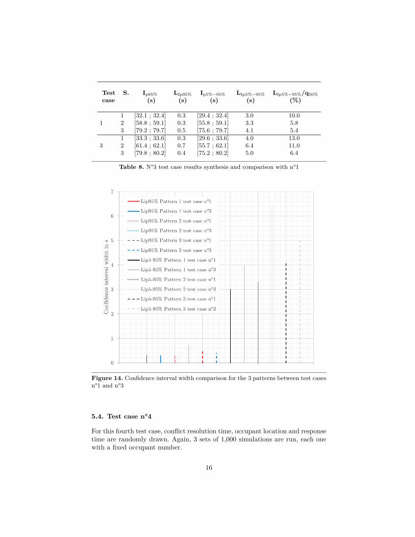
For this third test, conflict resolution time and occupants position are randomlydrawn. Again, 3 sets of 1,000 simulations are run, each one with a fixed occupantnumber.

Table 8 summarize the three simulations sets results and compares them ton°1 test case. The widths of interval are included in figure 14. It quantifies theinfluence of position. As could be expected,its influence is greater on the low andaverage densities of population than on a strong density.

15

Test S. Ip95% LIp95% Ip5%−95% LIp5%−95% LIp5%−95%/q50%case (s) (s) (s) (s) (%)

1 [32.1 ; 32.4] 0.3 [29.4 ; 32.4] 3.0 10.01 2 [58.8 ; 59.1] 0.3 [55.8 ; 59.1] 3.3 5.8

3 [79.2 ; 79.7] 0.5 [75.6 ; 79.7] 4.1 5.41 [33.3 ; 33.6] 0.3 [29.6 ; 33.6] 4.0 13.0

3 2 [61.4 ; 62.1] 0.7 [55.7 ; 62.1] 6.4 11.03 [79.8 ; 80.2] 0.4 [75.2 ; 80.2] 5.0 6.4

Table 8. N°3 test case results synthesis and comparison with n°1

Figure 14. Confidence interval width comparison for the 3 patterns between test casesn°1 and n°3

5.4. Test case n°4

For this fourth test case, conflict resolution time, occupant location and responsetime are randomly drawn. Again, 3 sets of 1,000 simulations are run, each onewith a fixed occupant number.

16

Table 9 summarize the three simulations sets results and compared to n°3test case. The intervals widths are presented in figure 15. The response timevariability strongly affects the RSET distributions patterns 2 and 3. The RSETminimum value increases for pattern n°1 when the variability is added to theresponse time. This may be caused by some few extreme cases drawn among the1,000 simulations.

Test P. Ip95% LIp95% Ip5%−95% LIp5%−95% LIp5%−95%/q50%case (s) (s) (s) (s) (%)

1 [33.3 ; 33.6] 0.3 [29.6 ; 33.6] 4.0 13.03 2 [61.4 ; 62.1] 0.7 [55.7 ; 62.1] 6.4 11.0

3 [79.8 ; 80.2] 0.4 [75.2 ; 80.2] 5.0 6.41 [36.9 ; 37.8] 0.9 [33.9 ; 37.8] 3.9 11.0

4 2 [61.4 ; 62.4] 1.0 [50.9 ; 62.4] 11.5 20.73 [82.3 ; 83.1] 0.8 [74.3 ; 83.1] 8.8 11.3

Table 9. N°4 test case result synthesis and comparison with n°3

Figure 15. Confidence interval width comparison for the 3 patterns between test casesn°3 and n°4

17

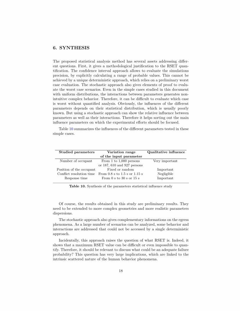
6. SYNTHESIS

The proposed statistical analysis method has several assets addressing differ-ent questions. First, it gives a methodological justification to the RSET quan-tification. The confidence interval approach allows to evaluate the simulationsprecision, by explicitly calculating a range of probable values. This cannot beachieved by a unique deterministic approach, which relies on a preliminary worstcase evaluation. The stochastic approach also gives elements of proof to evalu-ate the worst case scenarios. Even in the simple cases studied in this documentwith uniform distributions, the interactions between parameters generates non-intuitive complex behavior. Therefore, it can be difficult to evaluate which caseis worst without quantified analysis. Obviously, the influences of the differentparameters depends on their statistical distribution, which is usually poorlyknown. But using a stochastic approach can show the relative influence betweenparameters as well as their interactions. Therefore it helps sorting out the maininfluence parameters on which the experimental efforts should be focused.

Table 10 summarizes the influences of the different parameters tested in thesesimple cases.

Studied parameters Variation range Qualitative influenceof the input parameter

Number of occupant From 1 to 1,000 persons Very importantor 187, 610 and 927 persons

Position of the occupant Fixed or random ImportantConflict resolution time From 0.8 s to 1.5 s or 1.15 s Negligible

Response time From 0 s to 30 s or 15 s Important

Table 10. Synthesis of the parameters statistical influence study

Of course, the results obtained in this study are preliminary results. Theyneed to be extended to more complex geometries and more realistic parametersdispersions.

The stochastic approach also gives complementary informations on the egressphenomena. As a large number of scenarios can be analyzed, some behavior andinteractions are addressed that could not be accessed by a single deterministicapproach.

Incidentally, this approach raises the question of what RSET is. Indeed, itshows that a maximum RSET value can be difficult or even impossible to quan-tify. Therefore, it should be relevant to discuss what could be an adequate failureprobability? This question has very large implications, which are linked to theintrinsic scattered nature of the human behavior phenomena.

18

7. CONCLUSIONThe work presented here is a first step towards a statistical view on egressengineering. Is focuses on the quantified results given by the mathematical tools.There is still a lot of work to produce in order to get an engineering level tool.

First, the method developed here has been carried out by simple automationscripts. It should be enhanced and industrialized by using stochastic-dedicatedtools.

Furthermore, and maybe above all, the input data required by this methodstill have to be refined. The input parameters distributions should especially bestudied. As presented above, applying a stochastic approach can help sortingout the main influences, and prioritizing which evacuation tests to perform inorder to get these informations. This action requires deeper and more extensiveanalysis of the different behavior parameters, possibly using experimental plans.A comparison between various egress engineering tools parameters should alsobe carried out.

Finally, the quantitative precision and evaluation criteria given by this ap-proach can also help comparing simulations and experiments. It can also helpsetting up relevant test protocol in order to maximize the useful informationsamount produced by these tests. This kind of work seems achievable once a goodknowledge of the input parameters is available.

REFERENCES1.[1] Enrico Ronchi, Arturo Cuesta, and Steven M. Gwynne. Collection and Use of Data

from School Egress Trials. Interscience communications. 2015.2.[2] Rodrigo Machado Tavares, and Enrico Ronchi. Uncertainties in Evacuation Mod-

elling: Current Flaws and Future Improvements. Interscience communications. 2015.

19