stochastic backpropagation for coherent optical communication

Improving landfill monitoring programswith the aid of geoelectrical - imaging techniquesand geographical information systems Master’s Thesis in the Master Degree Programme, Civil Engineering

KEVIN HINE

Department of Civil and Environmental Engineering Division of GeoEngineering Engineering Geology Research GroupCHALMERS UNIVERSITY OF TECHNOLOGYGöteborg, Sweden 2005Master’s Thesis 2005:22

Stochastic Backpropagation for CoherentOptical CommunicationMaster’s Thesis in communication systems and information theory

YAN GONGNAN JIANG

Department of Signals & SystemsCommunication EngineeringChalmers University of TechnologyGothenburg, Sweden 2011EX081/2011

Abstract

We present stochastic backpropagation, a novel maximum a posteriori detection methodfor coherent optical communications with dual polarization and Multilevel quadratureamplitude modulation formats (M-QAM) transmission. The proposed detector is shownto outperform conventional backpropagation in a scenario where nonlinear phase noise isthe dominant impairment and polarization dependent loss (PDL) channels are existed.We also provide a novel channel estimation method for unitary channel effect and aML-based channel estimation method for PDL channel.

Acknowledgements

This thesis work has been performed at Chalmers in Gothenburg, Sweden, under thesupervision of Assistant Professor Henk Wymeersch. We would like to express our grat-itude to people who has been involved to sponsor and help us to complete our work.

First we would like to thank Assistant Professor Henk Wymeersch, who has guidedus with his brilliant advices and kept pushing us to further study. We would also like tothank PhD student Johnny Karout, who helped us a lot to solve all kinds of problemsin this thesis. Thanks to the help of Henk and Johnny, we released a paper in ECOCduring the thesis study and we are very proud of working with them. Another importantperson we would like to thank is master student Mehrnaz Tavan, who shared her researchachievement generously with us and helped us a lot in our later study.

Last but not least, we would like to thank all the friends of ours, who helped us alot not only in thesis study but also during the 2 years master study. We shared a lot ofgood time together here in Chalmers, thanks to all of you.

Yan Gong and Nan Jiang, Gothenburg 2011/9/11

Contents

1 Introduction 11.1 Coherent optical communication . . . . . . . . . . . . . . . . . . . . . . . 1

1.1.1 Nonlinear impairments . . . . . . . . . . . . . . . . . . . . . . . . . 11.1.2 Memoryless linear impairments . . . . . . . . . . . . . . . . . . . . 2

1.2 Thesis structure . . . . . . . . . . . . . . . . . . . . . . . . . . . . . . . . . 3

2 Literature Review 42.1 System model . . . . . . . . . . . . . . . . . . . . . . . . . . . . . . . . . . 4

2.1.1 Non-linear optical communication system . . . . . . . . . . . . . . 52.1.2 PDL channel . . . . . . . . . . . . . . . . . . . . . . . . . . . . . . 5

2.2 Previously research . . . . . . . . . . . . . . . . . . . . . . . . . . . . . . . 62.2.1 Previously research of SPM . . . . . . . . . . . . . . . . . . . . . . 62.2.2 Previously research of PDL channel . . . . . . . . . . . . . . . . . 8

2.3 Factor Graph and Monte Carlo technique . . . . . . . . . . . . . . . . . . 112.3.1 Factor Graph . . . . . . . . . . . . . . . . . . . . . . . . . . . . . . 112.3.2 Monte Carlo technique . . . . . . . . . . . . . . . . . . . . . . . . . 12

3 Data detection 143.1 Linear unitary channel . . . . . . . . . . . . . . . . . . . . . . . . . . . . 14

3.1.1 Channel estimation . . . . . . . . . . . . . . . . . . . . . . . . . . . 163.1.2 Data detection . . . . . . . . . . . . . . . . . . . . . . . . . . . . . 16

3.2 Non-linear unitary channel . . . . . . . . . . . . . . . . . . . . . . . . . . 173.2.1 Data detection . . . . . . . . . . . . . . . . . . . . . . . . . . . . . 18

3.3 Linear non-unitary channel . . . . . . . . . . . . . . . . . . . . . . . . . . 183.3.1 Channel estimation . . . . . . . . . . . . . . . . . . . . . . . . . . . 193.3.2 Data detection . . . . . . . . . . . . . . . . . . . . . . . . . . . . . 20

3.4 Non-linear non-unitary channel . . . . . . . . . . . . . . . . . . . . . . . . 223.4.1 Data detection . . . . . . . . . . . . . . . . . . . . . . . . . . . . . 22

i

CONTENTS

4 Performance analysis 234.1 Linear unitary channel . . . . . . . . . . . . . . . . . . . . . . . . . . . . 23

4.1.1 Simulation results and performance analysis . . . . . . . . . . . . . 234.1.2 Channel estimation results . . . . . . . . . . . . . . . . . . . . . . 25

4.2 Non-linear unitary channel . . . . . . . . . . . . . . . . . . . . . . . . . . 264.2.1 Simulation results and performance analysis . . . . . . . . . . . . . 264.2.2 Channel estimation results . . . . . . . . . . . . . . . . . . . . . . 28

4.3 Linear non-unitary channel . . . . . . . . . . . . . . . . . . . . . . . . . 284.3.1 simulation results . . . . . . . . . . . . . . . . . . . . . . . . . . . . 294.3.2 Performance analysis . . . . . . . . . . . . . . . . . . . . . . . . . . 29

4.4 Non-linear non-unitary channel . . . . . . . . . . . . . . . . . . . . . . . 324.4.1 Simulation results and performance analysis . . . . . . . . . . . . . 32

5 Conclusion 345.1 Unitary channel estimation . . . . . . . . . . . . . . . . . . . . . . . . . . 345.2 Non-unitary channel estimation . . . . . . . . . . . . . . . . . . . . . . . 345.3 Data detection with backpropagation . . . . . . . . . . . . . . . . . . . . 34

6 Future Work 366.1 Channel estimation for nonlinear non-unitary system . . . . . . . . . . . . 366.2 ISI . . . . . . . . . . . . . . . . . . . . . . . . . . . . . . . . . . . . . . . . 366.3 Other problems . . . . . . . . . . . . . . . . . . . . . . . . . . . . . . . . . 37

Bibliography 39

ii

1Introduction

Multilevel quadrature amplitude modulation formats (M-QAM) is widely used in thecoherent optical communication due to its ability to increase the spectral efficiency com-paring to the traditional optical communication. However, as the minimum distancedecreases on the constellation, M-QAM is more sensitive to the noise and requires morepower to reach a certain bit-error-rate (BER). Some other characters of optical systemwill also affect the results during the transmission, like high power will lead to increas-ing intrachannel four-wave mixing which causes the nonlinear inter-symbol interference(ISI), and self-phase modulation (SPM) [1].

This thesis is aimed to build a novel detector to solve both SPM noise and PDLchannel effect, the detector is built based on some techniques such as back propagation,factor graph (FG) and Monte Carlo technique. In this thesis, we focus on a dual po-larization 16-QAM system. The key components will be studied separately before thewhole system is taken into consider.

1.1 Coherent optical communication

Coherent technologies have been as a hot topic as the transmission-capacity increasesin wavelength-division multiplexed (WDM) systems [2]. In coherent optical communi-cation, signal is encoded onto the electrical filed of the light wave. Polarization is one ofthe main issues may take into consideration. A polarized signal is a wave which all theelectric components are in a fixed phase relationship. So phase and polarization are thekey obstacles for the implementation of the coherent receivers.

1.1.1 Nonlinear impairments

Both linear and nonlinear impairments are contained in optical communication model.Linear impairments include chromatic dispersion (CD) and polarization mode dispersion(PMD). Nonlinear impairments originate from Kerr effect, which is named after the

1

CHAPTER 1. INTRODUCTION

Scottish Physicist John Kerr. It refers to the phenomenon that the refractive index ofthe optical fiber varies as the launched power changes. Nonlinear impairments includeself phase modulation (SPM), cross phase modulation (XPM) and four wave mixing(FWM).

Self-phase modulation (SPM) is interesting to study since it only can be partiallycompensated while nonlinear inter-symbol interference (ISI) can be compensated for, asshown in [3]. SPM causes the signal to change its own phase while travelling throughthe fiber. In combination with amplified spontaneous emission (ASE) noise, SPM leadsto nonlinear phase noise (NLPN) [4], which in signal space can be viewed as symbolselongated in the phase direction [1]. In this thesis work, the chromatic dispersion (CD)is neglected so that NLPN is the dominant impairment for the communication system[1, 5, 6].

An experimental investigation has showed that NLPN is a limiting factor [7] andrecent results indicate that NLPN is important up to 40 Gbaud [8]. To mitigate theeffect caused by NPLN, compensation have to be made at the receiver side. A stochasticback propagation method based on factor graph and Monte carlo technique is studiedin this thesis to achieve the goal.

1.1.2 Memoryless linear impairments

Polarization dependent loss (PDL) channel is another dominant component which limitsthe system performance. Polarization dependent loss is the ratio of the maximum andthe minimum power amplitude to the all polarization states. It is usually caused bycircular dichrosim, fiber bending, angled optical interfaces or oblique reflection [9].

Each optical device exhibits a polarization dependent transmission, the polarizationchanges randomly over each fiber span. Generally, the PDL of each span cannot bedetermined by simply adding all the PDL components together in this case which isthe worst situation. The total PDL depends on the polarization transformation of eachspan. The BER of the system is highly affected by these. PDL is also the main sourceof pulse distortion [10].

In fiber optical transmission, the devices have PDL are fibers, optical couplers, iso-lators, WDM and photonic-detectors. The PDL of each component are different, it maydepend on the input wavelength of the source. The polarization along the fiber is unpre-dictable and uncontrolled which will lead to the decrease of the quality of fiber opticaltransmission. Therefore, the systems always require the device with the low PDL.

Consequently, the measurement of PDL has become a hot topic and attracted lotsof attention from manufacturers and researchers. The perfect estimation can highlyimprove the quality of transmission.

Erbium-doped fiber amplifier (EDFA) is the most common amplifier that is used inthe fiber optical communication. EDFAs use a doped optical fiber as a gain mediumto amplify an optical signal. EDFAs have two major pumping bands 980 nm and 1480nm. The 980 nm band has a higher absorption cross-section and is used in the low noisesituation, on the contrary, the 1480 nm band has a lower absorption cross-section andused when high power is required.

2

CHAPTER 1. INTRODUCTION

Additive white Gaussian noise (AWGN) is an ideal channel model in which theadded noise is wideband with constant spectral density and a Gaussian distribution ofamplitude. The AWGN channel is a good model deep space communication links. It isnot good for most terrestrial links because of multipath or interference. But AWGN iscommonly used to simulate background noise of the channel.

1.2 Thesis structure

After the introduction, we will give the system model we studied in this thesis, also withthe abstract of previously research achievements of coherent optical communication. Thedetails of factor graph and Monte Carlo technique are also contained in chapter 2.

Chapter 3 includes most parts of achievements in this thesis. We divided the wholesystem into several key components and solve the problems separately. In the end, adetector designed for the entire system will be built.

We present the results in chapter 4, analyze the performance by comparing the resultswith some known methods and different simulation parameters.

Chapter 5 is the conclusion of this thesis study, followed by chapter 6, the futurework.

3

2Literature Review

In this chapter we will give all the basic knowledge for our study, including systemmodel, channel character, introduction of backpropagation, factor graph and MonteCarlo technique, along with some previously research achievements of SPM and PDLchannel.

2.1 System model

TX

span

RX

n SPM

loss

amplifierfiber

PDL

Figure 2.1: Optical transmission model

We consider a discrete-time multi-span polarization multiplexed coherent opticalcommunication system with optical dispersion compensation. The system model is givenin Figure 2.1. The long-haul transmission system contains many spans like this. At eachsymbol period, we transmit a two-dimensional complex data vector a, a is drawn uni-formly from a constellation Ω2 with average energy proportional to the input power Pinper polarization.

Optical communication system consists of a single mode fiber (SMF) followed by adispersion compensating fiber (DCF) and an amplifier in each span. SMF and DCFhave two Kerr nonlinear parameters and two attenuation factors αsmf , αdcf . The DCF

4

CHAPTER 2. LITERATURE REVIEW

is assumed to ideally compensate for the chromatic dispersion [1]. The signal power isattenuated by e−ξ = e−(αsmfLsmf+αdcfLdcf) where Lsmf and Ldcf are the lengths of SMF andDCF. The amplifier has a power gain G = e−ξ, in order to restore the signal power to thelevels in the transmitter side. The amplifier generates an amplified spontaneous emission(ASE) noise, which can be modeled as an additive white Gaussian noise (AWGN) process.The PDL channel exists between SPM and AWGN.

SPM, PDL channel and AWGN are three major components in this system. As weare familiar to deal with additive white Gaussian noise, we focus our study on SPM andPDL channel. To make the problem more clear, we isolate the nonlinear part and thechannel, then discuss them separately.

2.1.1 Non-linear optical communication system

TX RX

n

NL

Figure 2.2: Simplified transmission model for 1 span

If we only take SPM and AWGN into account, we can redraw the transmission systemfor one span like Figure 2.2. The NL block represent the SPM effect of the fiber and nis the ASE noise. The discrete-time signal at the output of the i-th span will be givenby

ri(t) = ri−1(t) exp(jγLeff ‖ri−1(t)‖2

)+ ni(t), (2.1)

where r0(t) = s(t). For clarity, SPM is neglected in the DCF1, so γ = γsmf as γsmf is thenonlinearity parameter of SMF, Leff is the effective length of the fiber, which is writtenas Leff =

(1− e−αL

)/α, in which attenuation factor α = αsmf and length L = Lsmf , the

operator ‖ · ‖ represents the norm given by ‖x‖ :=√xHx and ni(t) is ASE noise, which

is modeled as a zero-mean and has power spectral density of N0 per polarization, thenoise is bandlimited to a bandwidth B.

2.1.2 PDL channel

Polarization dependent loss is defined as:

PDLdB = 10× log(PMax

PMin), (2.2)

1The input power to the DCF is low, so SPM is neglected.

5


In practical PDL channel is defined as:

HPDL = U×

[1 0

0 γ

]×UH, (2.3)

where U is a random unitary matrix2, γ3 is the polarization dependent attenuationfactor, it is in the range of 0 to 1, usually around 1.

This channel has several properties. The γ matrix is a diagonal matrix. When γequals to 1, the PDL channel will no longer exist, as unitary matrix times its hermitianis an identity matrix. This can be used to check if the channel estimation works well.Another property is that γ cannot be 0, in this thesis, we focus on the dual polarization,there are always two lines of signals transporting together, if γ is zero, there will beunexpected mistake.

The PDL channel is added in each span of the fiber. Our task is to estimate andequalize the channel through numbers of spans with the nonlinear phase noise effect. Inour study, γ is considered as a constant for each span which value is near 1.

2.2 Previously research

As the new technology like erbium-doped fiber amplifier (EDFA), WDM and fiber non-linearity management breakthrough, the capacity of the fiber has been growing fast inpast years. Meanwhile, the spectral efficiency for optical communication has also beenincreasing.

In order to achieve high spectral efficiency, the study of coherent optical communica-tions has attracted the attention from all over the world. The coherent optical receivershave following advantages: by using phase modulation, the multilevel modulation formatcan be introduced; the receiver sensitivity has improved since the ability of the phasedetection increased; the closely spaced WDM channels can be separated at the electricallevel as the frequency resolution at baseband is high; the local oscillator power can helpto achieve the shot-noise limited receiver sensitivity.

These are all attribute to the rapid growth of high-speed digital signal processing(DSP). By using DSP, both the phase and polarization management can be done.

2.2.1 Previously research of SPM

Many studies have been done to analyze the effect of nonlinear phase noise and differentmethods have been brought to mitigate the effect of NLPN at the receiver, includingdifferent kind of compensation technique, MAP and ML detection and backpropagation.Here we give a brief review of several typical methods.

2A unitary matrix has the character that U×UH = UH ×U = I, where I is an identity matrix andUH is the Hermitian adjoint of U, both U and UH are square matrix

3For clarity, in this thesis γ represents the nonlinear parameter and γ represents the PDL factor

6


Electronic compensation technique

Optimal compensation using electronic circuits to mitigate NLPN for binary phase-shiftkeying (BPSK) and differential quadrature phase-shift keying (DQPSK) was proposedin [5]. In their study, the overall nonlinear phase shift is equal to:

ΦNL = γLeff|E0 + n1|2 + |E0 + n1 + n2|2 + · · ·+ |E0 + n1 + n2 + · · ·+ nN|2, (2.4)

where E0 is the transmitted signal, nk is the complex amplifier noise at the kth span, γis the nonlinear coefficient of the fiber and Leff is the effective length of the fiber. Theyuse a an optical phase-locked loop (PLL) in PSK system and a pair of interferometers inDPSK to receive the in-phase and quadrature components of the received electric field.They derived optimal compensator by finding a scale factor β which can minimize thevariance of the residual nonlinear phase shift ΦNL+βPN . The corrected phase estimateis ΦR − βPN , where ΦR is the phase of the received electric field ER [5]. The optimalscale factor is found to be

β = −γLeffN + 1

2· |E0|2 + (2N + 1)σ2/3

|E0|2 + Nσ2≈ −γLeff

N + 1

2. (2.5)

In their research, optimal compensation can halve the standard deviation (STD) of thenonlinear phase noise, doubling the transmission distance in systems whose dominantimpairment is nonlinear phase noise [5]. Their method was extended to M -ary phase-shift keying in [6].

Close-form detector

In [1], a close-form detector was derived for a polarization-multiplexed M-QAM systemwith discrete amplification, limited by NLPN. The detector is based on maximum like-lihood (ML) detection. They use the same system model as we mentioned in 2.1.1 andget the receive signal for Na span by recursive calculation:

rk = sk exp

(jγLeff

Na−1∑i=0

‖ri,k‖2)

+ wk, (2.6)

where sk =√Pinak (assuming negligible inter-symbol interference), wk ∼ CN (0,Naσ

2ASEI),

and σ2ASE = BN0 [1]. They derived the approximate likelihood function and used it as

a detector, which is given by

ak = arg maxak∈Ω2

p(rk|ak) (2.7)

= arg maxak∈Ω2

exp

(− ‖sk‖

2

Naσ2ASE

)I0(|βk|)

I0(1/σ2ψ). (2.8)

where I0(.) is the zeroth order modified Bessel function of the first kind, and

βk =2rHk ske

(jγLeffNa‖sk‖2+jφ)

Naσ2ASE

+1

σ2ψ

. (2.9)

7


whereφ = γLeffσ

2ASE(Na − 1)Na/2, (2.10)

andσ2ψ = 2γ2L2

eff ‖sk‖2 σ2

ASE(Na − 1)Na(2Na − 1)/6, (2.11)

In their research, the closed-form detector provides the best complexity-performancetrade-off compared with a number of suboptimal detectors and a complex non-parametricdetector.

Adaptive MAP detection

An adaptive maximum a posteriori (MAP) detection scheme was investigated in [11].They studied the performance of a MAP detection scheme with a look-up table for non-linear inter-symbol interference compensation and showed that MAP detection can helpto increase spectral efficiency and improve nonlinearity tolerance in long-haul transmis-sions [11].

Digital backpropagation

Backpropagation was proposed as a universal technique for jointly compensating lin-ear and nonlinear impairments in [12] and [13]. The use of digital backpropagation inconjunction with coherent detection to mitigate fiber nonlinearity and dispersion jointlyis studied in [3]. They proposed a solution of the inverse nonlinear Schroinger equa-tion (NLSE) by using noniterative asymmetric split-step Fourier method (SSFM). BPhas been shown to enable higher launched power and longer system reach in densewavelength-division-multiplexed (WDM) transmission over zero-dispersion fiber [12].

Backpropagation learning algorithm contains two parts: propagation and weight up-date. Each propagation involves forward propagation and backward propagation. In thisthesis, forward propagation is the transmission process and the backward propagation isthe detection process. By using backpropagation, we can detect the original transmittedsignals from the receive signals. To achieve this goal, we need to analyze the transmissionsystem and calculate the update weight. This is done by using factor graph and MonteCarlo techniques.

In this thesis, we compare our detector with a backpropagation detector. The back-propagation detector only considers the deterministic part of the nonlinearity whileignore the effects in nonlinear part caused by AWGN noise. The system model isr = s exp(jγLeffNa ‖s‖2) + n, the detector is given by

ak = arg minak∈Ω2

∥∥∥rk − sk exp(jγLeffNa ‖sk‖2)∥∥∥2. (2.12)

2.2.2 Previously research of PDL channel

The research and development in optical fiber communication started around 1970s [2].There are two basic methods to measure PDL of the device, the polarization scanning

8


technique and the Mueller method. At some specific wavelengths polarization scanningtechnique is more suitable. For a wavelength range, the Mueller method gives a betterperformance.

Polarization scanning technique

The polarization scanning technique is a non-deterministic method based on the mea-surement of the maximum and minimum power amplitude. The device under test (DUT)is exposed to all stated of polarization state. The polarization is controlled by a polar-ization controller that can be deterministically or randomly. Then the maximum andminimum is measured over time. And the PDL is calculated by its definition. But wecannot tell when there is a change, whether it caused by the PDL of the DUT or theinput power of the device.

In order to get a precise measurement, the input power must be stable, the sourcemust have high degree of polarization, the loss in the polarization controller must besmall, also the detector must have low polarization dependent responsitivity, as thesewill largely influence the detection of the PDL.

In practical, the errors from the scanning time and the measuring time are limited,which means the longer the polarization scanning takes, the more accurate the measure-ment of PDL is.

Besides setting the scanning time, it is important to set a correct scanning rate aswell. The faster scanning rate will generate more polarization state then the measuringtime will decrease. But if the rate is too fast, the results may get worse.

Mueller method

Mueller method is a different approach from polarization scanning technique, as it is adeterministic method and measures the PDL of a DUT from its Mueller matrix.

Mueller method only exposes the source to four polarization states, linear horizontalpolarized (LHP), linear vertical polarized (LVP), linear +45 degrees (L +45), right handcircular (RHC). PDL is calculated from the information obtained by these states.

The Mueller matrix indicates the polarization and power properties of the DUT. Therelationship between input Stokes vector, output Stokes vectors and the Mueller matrixis

Sout = M× Sin, (2.13)

The Mueller matrix is a 4 by 4 matrix. The first row coefficients of the Muellermatrix describe the total optical power are required in calculating the PDL of the DUT.

S = m11S0in + m12S1in + m13S2in + m14S3in, (2.14)

9


where m11...m14 are the first row coefficients, and input Stokes Vectors are:

LHP : S0in =

Pin1

Pin1

0

0

LVH : S1in =

Pin2

−Pin2

0

0

L+45 : S2in =

Pin3

0

Pin3

0

RHC : S3in =

Pin4

0

0

Pin4

,(2.15)

Output Stokes Vectors for four polarizations are:

Pout1 = m11Pin1 + m12Pin2 (2.16)

Pout2 = m11Pin1 −m12Pin2

Pout3 = m11Pin3 + m13Pin3

Pout4 = m11Pin4 + m14Pin4.

Determining all the power values needs following steps. First, four polarization statesmust be taken measurement individually, in order to get the different input powers.Second, the DUT is inserted and the output powers corresponding to four polarizationstates must be recorded.

It should be noticed that the power and wavelength for PDL measurement must bein the same condition.

Solving the equation system for m11...m14 of the Mueller matrix yields:

m11

m12

m13

m14

=

12

(Pout1Pin1

+ Pout2in2

)12

(Pout1Pin1

− Pout2in2

)Pout3Pin3

−m11

Pout4Pin4

−m11

, (2.17)

Then the maximum and minimum transmissions through DUT can be derived as:

PMax = m11 +√

m212 + m2

13 + m214 (2.18)

PMin = m11 −√

m212 + m2

13 + m214,

By the definition, the PDL of the DUT can be calculated.The Mueller method has some specific requirements on the polarization controller.

It helps to generate four polarization states. It contains a polarizer and a retarder.The polarizer generates the linear polarization state, and the rotation of the retardergenerates other polarization states. The angular of the controller will affect the accurateof the measurement.

The polarization controller also provides some loss. It will affect the measurement ofthe reference power.

10


Comparison

Generally, the polarization scanning technique is suitable for PDL measurement for singlewavelength, and the Mueller method is capable for a wavelength range. The polarizationscanning technique exposes the source to all the polarization states, so it can measurethe PDL at a certain wavelength at one time. And it is easy to implement and doesn’ttake too complicated math work. On the contract, the Mueller method requires manywavelength points, it suitable for several channels.

In this thesis, we only have to take care of the PDL channel, which means the PDLis known to us. And we neglect all the noise introduced by the devices to simplify thesimulation.

2.3 Factor Graph and Monte Carlo technique

As we mentioned above, factor graph and Monte Carlo technique are two very importanttechniques in this thesis, almost all the research works are based on them. We use factorgraph to analysis the transmission system and use Monte Carlo technique to calculatethe results of backpropagation. Before we can start derive the detector, we need to givesome introductions for these two techniques.

2.3.1 Factor Graph

Factor graph is a particular type of graphical model that represents the factorization ofa function. Suppose there is a function f : X1 × X2 × · · · × XN → R, which is factorizedto K factors,

f(x1,x2,...,xN) =K∏k=1

fk(sk), (2.19)

where fk(·) is a real-valued function and sk ⊆ x1,x2,...,xN is the kth variable subset.The factor graph of this factorization is created as follows. First, We create an edge(drawn as a line) for every variable, and a node (drawn as a circle or a square) for everyfactor. If a certain variable appears in a certain factor, we attach the corresponding edgeto the corresponding node. In our study, an edge can be attached only to two nodes,which means there is no branch in the factor graph in this thesis.

TX

n SPM

loss

ampli!er!ber

a x1 r1 x2 r2

RX

n SPM

loss

ampli!er!ber

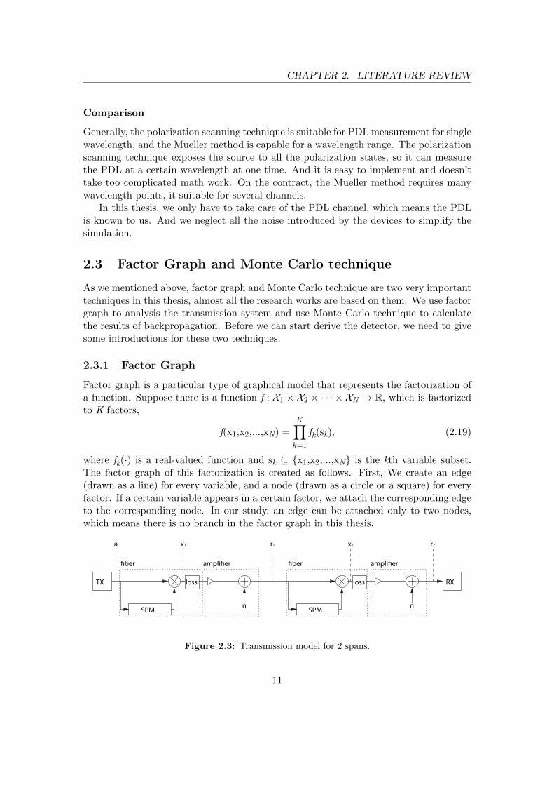
Figure 2.3: Transmission model for 2 spans.

11


If we substitute f(·) and fk(·) with probability density functions, we can get thecorresponding factorized representation of a certain distribution. For the system modelgiven by Figure 2.3,(where the PDL channel is ignored) the factorization representationof the distribution p(a,x1,r1,x2|r2) is given by

p(a,x1,r1,x2|r2) ∝ p(a)p(x1|a)p(r1|x1)p(x2|r1)p(r2|x2), (2.20)

where ∝ denotes quality up to a multiplicative constant. The corresponding factor graphis shown in Figure 2.4.

Figure 2.4: Factor graph of p(a,x1,r1,x2|r2).

The arrow refers to the messages which are computed as follow: given a factor f(·)with variables x and y, and an incoming message m(x), then the out going message isgiven by

m(y) = C

∫f(x,y)m(x)dx, (2.21)

where C is a normalization constant and the integration interval is the domain of x. Somefactors may only have one variable (the factors on the boundary), if so, m(y) = Cf(y) (ify is the only variable).

2.3.2 Monte Carlo technique

Monte Carlo techniques gives an innovation method to solve complex integration andoptimization compare to traditional Bayesian estimation. The essential idea is represent-ing distributions as a list of samples on which integration and optimization are based.The definition of particle representation is given as follows: suppose we have a randomvariable Z which defined over a set Z. A particle representation of a distributionpZ(z)is a set of L couples (w(l),z(l)), with Σlw

(l) = 1, for any integrable function f(z) fromZ → C,

I = EZf(Z), (2.22)

can be approximated by

IL =L∑l=1

w(l)f(z(l)), (2.23)

where z(l) is named a properly weighted sample with weight w(l).

12


Then we introduce an alternative notation for continuous Z:

pZ(z) ≈L∑l=1

w(l)δ(z− z(l)), (2.24)

where δ(·) is the Dirac distribution. On the contrary, the notation of discrete Z is givenby

pZ(z) ≈L∑l=1

w(l)Iz = z(l), (2.25)

where, for a proposition X, IX is the indicator function, defined as IX = 1 whenX is true and IX = 0 when X is false. With Mote Carlo technique, we can easilycompute the expectation EZf(Z).

13

3Data detection

In this thesis, we simulate a coherent optical communication system of dual polarization16-QAM by using FG, Monte-Carlo technique and back propagation. We simplify theproblem by dividing the complicated system into separate components and organizedthe process in four steps.

3.1 Linear unitary channel

First, we build a simple transmission system by ignoring both the nonlinear noise andPDL channel effect. This can considered as the nonlinear parameter γ = 0 and thePDL channel is simplified to a unitary channel. Using this simplified model, we givea solution of channel estimation and data detection by factor graph and Monte Carlotechnique. These estimation and detection methods are the bases of this thesis. Themodel is a transmission system with linear noise and unitary channel effects, which isshown in Figure 3.1.

TX U1

n1

RXU2

n2

Figure 3.1: System model for 2 spans

The U block represent the unitary channel and n is the ASE noise of the fiber. Foreach span, the unitary channels are independent and different. Since the optical channelvaries slowly, we treat the unitary channel as constant matrix in our simulation.

14

CHAPTER 3. DATA DETECTION

Assuming that the original signal is s0, the output of the first span x1 is given by

x1 = U1(s0 + n1) (3.1)

= U1s0 + U1n1, (3.2)

where U1 is the unitary channel of the first span and n1 is the corresponding ASEnoise. In 3.2, we can calculate the mean and variance of U1n1. Since n1 has zero meanand a variance varn1, the expectation of U1n1 is EU1n1 = EU1En1 = 0, thevariance of U1n1 is varU1n1 = E(U1n1)2− (EU1n1)2, where EU1n1 = 0 and(U1n1)2 = nH

1 UH1 U1n1 = n2

1, so varU1n1 = En21 = varn1. After the derivation

above, we can conclude that U1n1 is still an additive white Gaussian noise with thesame mean and variance of n1, then 3.2 can be simplified to

x1 = U1s0 + n1, (3.3)

Then the output of the second span x2 is given by

x2 = U2(x1 + n2) (3.4)

= U2(U1s0 + n1 + n2) (3.5)

= U2U1s0 + n1 + n2, (3.6)

where we also use the conclusion above. In 3.6, U2U1 is still a unitary matrix since(U2U1)H(U2U1) = UH

1 UH2 U2U1 = I. So 3.6 can be rewrite as

x2 = Us0 + n1 + n2, (3.7)

where U = U2U1 is a unitary matrix. We can easily extend the result to k-th span:

xk = Us0 + n1 + n2 + · · ·+ nk (3.8)

= U(s0 + U(n1 + n2 + · · ·+ nk)) (3.9)

= U(s0 + n1 + n2 + · · ·+ nk), (3.10)

where U = Uk . . .U2U1, here we use the character that UH is also a unitary matrixto derive 3.10. Now the system model for k spans is reorganized as Figure 3.2.

TX RXU

n

Figure 3.2: Simplified system model for k spans

The system model for k spans is exactly the same as for 1 span, the only differencesare the values of noise n and channel U. In this model, n = n1 + n2 + · · · + nk andU = Uk . . .U2U1.

15


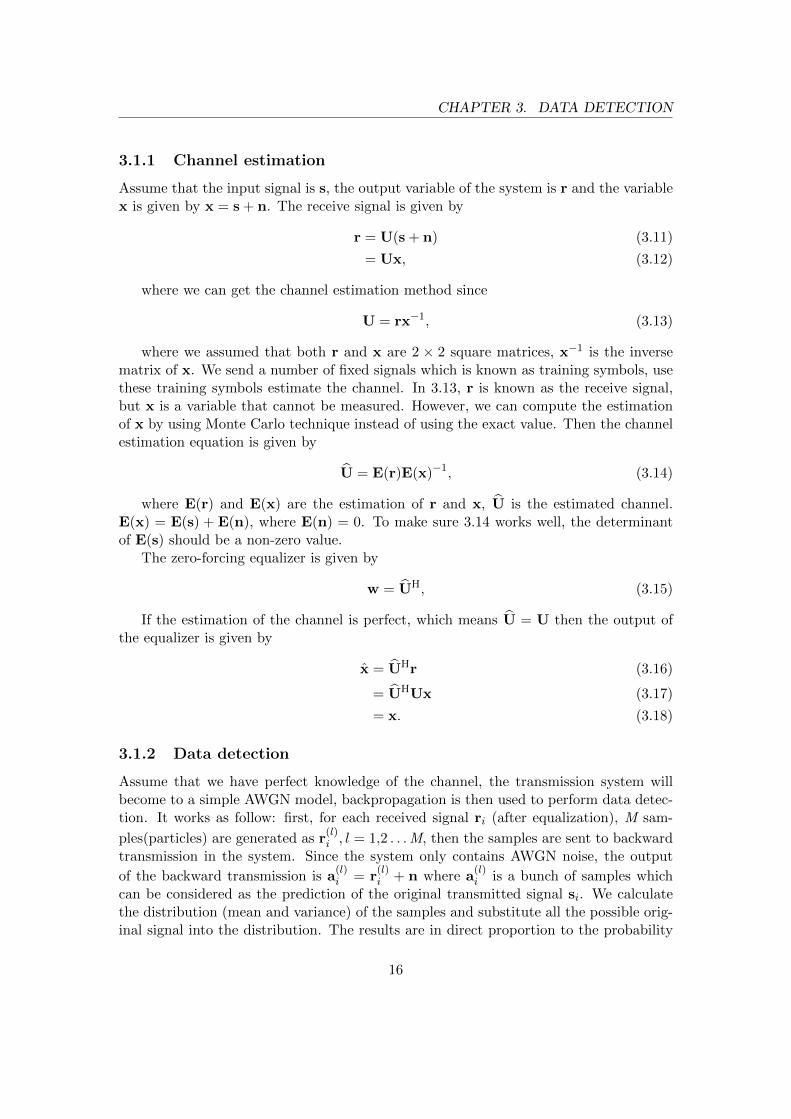
3.1.1 Channel estimation

Assume that the input signal is s, the output variable of the system is r and the variablex is given by x = s + n. The receive signal is given by

r = U(s + n) (3.11)

= Ux, (3.12)

where we can get the channel estimation method since

U = rx−1, (3.13)

where we assumed that both r and x are 2 × 2 square matrices, x−1 is the inversematrix of x. We send a number of fixed signals which is known as training symbols, usethese training symbols estimate the channel. In 3.13, r is known as the receive signal,but x is a variable that cannot be measured. However, we can compute the estimationof x by using Monte Carlo technique instead of using the exact value. Then the channelestimation equation is given by

U = E(r)E(x)−1, (3.14)

where E(r) and E(x) are the estimation of r and x, U is the estimated channel.E(x) = E(s) + E(n), where E(n) = 0. To make sure 3.14 works well, the determinantof E(s) should be a non-zero value.

The zero-forcing equalizer is given by

w = UH, (3.15)

If the estimation of the channel is perfect, which means U = U then the output ofthe equalizer is given by

x = UHr (3.16)

= UHUx (3.17)

= x. (3.18)

3.1.2 Data detection

Assume that we have perfect knowledge of the channel, the transmission system willbecome to a simple AWGN model, backpropagation is then used to perform data detec-tion. It works as follow: first, for each received signal ri (after equalization), M sam-

ples(particles) are generated as r(l)i , l = 1,2 . . .M, then the samples are sent to backward

transmission in the system. Since the system only contains AWGN noise, the output

of the backward transmission is a(l)i = r

(l)i + n where a

(l)i is a bunch of samples which

can be considered as the prediction of the original transmitted signal si. We calculatethe distribution (mean and variance) of the samples and substitute all the possible orig-inal signal into the distribution. The results are in direct proportion to the probability

16


p(si|ri) which means the signal gives the maximum value of the distribution function isthe result of the detection. Our detector is called stochastic backpropagation.

Here we discuss a little bit of the number M , generally speaking, the bigger M isthe better result we get since more information of the function are collected from theparticles. However, the result varies very slowly after M reaches a certain number1. Thesystem will be become less efficiency if we continue increase M and will not give goodperformance if M is not big enough.

3.2 Non-linear unitary channel

After simulated the system of linear noise and unitary channel effect, we built a systemcontains the nonlinear part and white Gaussian noise with the unitary channel effect. Itcan be considered as we change the nonlinear parameter γ from 0 to a non-zero constant.The system model is shown in Figure 3.3.

TX U1

n1

NL1 RXU2

n2

NL2

Figure 3.3: System model for 2 spans

Assuming that the original signal is s0, the output of the first span x1 is given by

x1 = U1(s0 exp(jγLeff ‖s0‖2) + n1) (3.19)

= U1s0 exp(jγLeff ‖s0‖2) + n1, (3.20)

In 3.20, we used the conclusion from the above section that U1n1 = n1. The outputof 2 spans is then given by

x2 = U2x1 exp(jγLeff ‖x1‖2) + n2, (3.21)

If s1 , s0 exp(jγLeff ‖s0‖2)+n1, then x1 = U1s1 and ‖x1‖2 = ‖U1s1‖2 = (s1)HUH1 U1s1 =

(s1)Hs1 = ‖s1‖2. So 3.21 can be rewrite as

x2 = U2U1s1 exp(jγLeff ‖s1‖2) + n2 (3.22)

= U(s1 exp(jγLeff ‖s1‖2) + n2

), (3.23)

where U = U2U1. From the derivation above, we find that unitary channel has noeffect on nonlinear noise, so we reorganize the system model as Figure 3.4.

U is the only channel effect in the system and we use the same method as above toestimate it.

1In this thesis, M = 100 is considered to be sufficient

17


TX RX

n1

NL1 NLk

nk

U

Figure 3.4: System model for k spans


Assume that we have the perfect knowledge of the unitary channel, the only problemleft is how to deal with the nonlinear noise. With stochastic backpropagation tech-nique, we compensate the nonlinear noise for each span. The nonlinear noise can beconsidered as a rotation in constellation without changing the signal energy. For a non-linear component rk = sk exp(jγLeff ‖sk‖2), the original signal sk can be regenerated assk = rk exp(−jγLeff ‖rk‖2). As we said above, the nonlinear noise will not change thesignal energy which means ‖sk‖2 = ‖rk‖2.

Combining the methods we gave in linear noise system, we can describe the backpropagation method as follow. After channel equalization, we generate particles for eachreceived signal rk then send the particles to backward transmission. For each span, thetransmission model is xk = rk + n, ak = xk exp(−jγLeff ‖xk‖2). After the transmissionprocess is finished, we can get the prediction of the original transmitted signal. Thedetection method is same as we provide in the first section.

In this step, we compare our method with two existed techniques, the regular maxi-mum likelihood (RML) detector and the back propagation method we provided in chap-ter 2. The RML detector simply ignores the nonlinear noise, considers the system asrk = sk + n. The detector is given by

ak = arg minak∈Ω2

‖rk − sk‖2 , (3.24)

3.3 Linear non-unitary channel

The third step is mainly about the estimation for PDL channel. The system we discussedhere only consist channels and white Gaussian noise. For each span the signal goesthrough the channel first then the noise is added. The signal is dual polarization QPSK.The original signal is s0, the polarization dependent attenuation factor γ for PDL isfixed and all the channels have the same value. Figure 3.5 shows the system model fortwo spans.

18


Figure 3.5: System model for 2 span

3.3.1 Channel estimation

The signal passed the first channel is

r1 = H1s0 + n1, (3.25)

where H1 is the first channel and n1 is the added noise with noise covariance matrixN0/L, N0 is the noise variance, L is number of spans. In our simulation, N0 is 1, L is 22.

The signal passed the second channel is

r2 = H2r1 + n2 = H2H1s0 + (H2n1 + n2) , (3.26)

The noise covariance matrix for this case is

(H2n1 + n2)× (H2n1 + n2)H (3.27)

= (H2n1 + n2)×(nH

1 HH2 + nH

2

)= H2

(N0

L

)HH

2 +N0

L,

So the signal after passing i-th span is

ri = Hiri−1 + ni, (3.28)

and the noise covariance matrix is

Σ = Hi...H2

(N0

L

)HH

2 ...HHi + ...+ Hi

(N0

L

)HHi +

N0

L, (3.29)

the total channel we wish to estimate is the multiplication of all the channel per span,the total channel is

Htotal = HiHi−1...H2H1, (3.30)

The noise covariance matrix has an interesting property. After passing 22 of spans,

it is nearly stable. After simulation, when γ equals to 0.99, Σ is around

[0.9 0

0 0.9

],

when γ equals to 0.9, Σ is around

[0.4 0

0 0.4

].

19


We use maximum likelihood function of the posteriori probability to estimate thechannel. The original dual polarization signal is jointly Gaussian, so the maximumlikelihood function is

r = arg max p(r|Htotals0) = (r−Htotals0)HΣ−1(r−Htotals0), (3.31)

where r is the received signal, s0 is the original signal, Σ is the noise covariance matrix,Htotal is the total channel we have to estimate. The function derives:

r = arg max p(r|Htotals0) (3.32)

= rHΣ−1r + sH0 HH

totalΣ−1Htotals0 − sH

0 HHtotalΣ

−1r− rHΣ−1Htotals0,

In order to maximum the function, we take the derivatives of this function, and setit equals to 0 to calculate the estimated channel. And according to the simulation, thenoise covariance matrix Σ can be considered as a fixed matrix β. So the function can bewritten as

∂ arg max p(r|Htotals0)

∂Htotal= 0 (3.33)(

(β−1)H

+ β−1)

Htotals0sH0 =

((β−1)

H+ β−1

)rsH

0 ,

So the estimated channel isHesti = rs0(s0s

H0 )−1, (3.34)

It is just a function of received signal and original signal, doesn’t relate to the noise.And the estimated channel is a scaled identity matrix.


We presented two kinds of equalizers, zero forcing (ZF) equalizer and minimum meansquare error (MMSE) equalizer in detecting the data.

Zero forcing (ZF) equalizer simply applies the inverse of the channel to the receivedsignal. It is a form of linear equalization which is widely used in the communicationsystems[14]. For the estimated channel Hesti, CZF is the equalization matrix, it is definedas

CZF = Hesti−1, (3.35)

It should be noted that, ZF equalization is not suitable for most applications, as eventhe channel impulse has finite length, the impulse response of the ZF equalizer is infinite;and ZF equalizer neglects the effects of the noise.

Minimum mean square error (MMSE) equalizer may be a better solution. MMSEequalizer minimizes the mean square error (MSE) of the transmitted data. MSE is arisk function. It is related to the expectation of the squared error loss, and measures theaverage of the square errors. It is defined as[14]

CMMSE =HH

esti

‖Hesti‖2 + Σ2

σs2

, (3.36)

20


where Σ is the noise covariance matrix, which is considered to be a fixed matrix and canbe obtained from the simulation. σs

2 is the variance of the modulated symbols.In the general cases, the MMSE equalizer should have a better performance than the

ZF equalizer, as the MMSE equalizer takes the effects of the noise into consideration. Butin the multi-spans PDL channel, these two equalizers have nearly the same performancewhen estimating the same channel under the same circumstance. This may due to thenoise.

We built a similar system to check this assumption. Instead of passing the channelfirst, the signal is firstly added the noise then passing the PDL channel. So the receivedsignal after passing the first span is rewritten as

r1 = H1(s0 + n1), (3.37)

so now the noise covariance matrix is H1

(N0L

)HH

1 .The signal passing the second span is

r2 = H2(r1 + n2) = H2H1s0 + (H2H1n1 + H2n2), (3.38)

and the noise covariance matrix is

(H2H1n1 + H2n2)× (H2H1n1 + H2n2)H (3.39)

= (H2H1n1 + H2n2)× (nH1 HH

1 HH2 + nH

2 HH2 )

= H2H1

(N0

L

)HH

1 HH2 + H2

(N0

L

)HH

2 ,

The received signal after passing the i-th span is

ri = Hi(ri−1 + ni), (3.40)

the noise variance matrix Σ for the total system is

Σ = Hi...H1

(N0

L

)HH

1 HHi + ...+ HiHi−1

(N0

L

)HHi−1HH

i + Hi

(N0

L

)HHi , (3.41)

The channel is estimated in the same way by using the same calculation, the estimatedchannel is still

ˆHesti = rs0(s0sH0 )−1, (3.42)

and the Σ is still nearly a fixed matrix after passing several spans.In this case, the performance of the MMSE equalizer has a clear improvement, is

much better than the ZF equalizer. Comparing with the previous case, we can easilyfigure out that the difference in the noise covariance matrix Σ is the key issue.

In the second case, each component of the Σ matrix is affected by the first thechannel. The noise will contribute more in the transmission. Since the MMSE equalizeris an estimation dealing with the noise. So the estimation in the second case for MMSEequalizer is better.

21


Since the ZF and MMSE equalizer has the same performance, we may implement ZFequalizer in practical, as it is easier to apply and has less computing complexity.

In both cases, the regular maximum likelihood (ML) detector is implemented to checkthe BER of the transmission.

Besides, the quality of transmission largely depends on the value of polarizationdependent attenuation factor γ. When γ is high, near 1, the BER can easily reach 0.001,that is the reason that we all wish the attenuation of the channel to be less.

3.4 Non-linear non-unitary channel

In the end, the nonlinear noise is added to the non-unitary system, the system modelfor 1 span is shown in Figure 3.6.

TX RXPDL

n

NL

Figure 3.6: System model for 1 span

The NL block is the nonlinear phase noise, the PDL block represents the PDL channeleffect, n is the AWGN noise. The PDL channel is the multiplication of a random unitarymatrix, an attenuation Γ matrix and the hermitian of the unitary matrix.


The channel estimation here is a little bit different here. since the nonlinearity and the Γmatrix is existed, we can not apply the method we provided in the previous section. Dueto the limitation of research period, we only provide the data detection method here.

Assuming that we have the prefect knowledge of the PDL channel, which means weknow not only the value of Γ, but also every unitary matrix in each span. With thestochastic backpropagation technology, the detection part is almost the same with thenon-linear unitary channel, the only difference is there is a PDL channel component ineach span. We generate bunch of samples from the backward transmission, and then thedistribution of these samples were calculated. The original signals are then substitutedto the distribution. The maximum value indicates the most probably prediction.

22

4Performance analysis

Here we discuss the numerous results, like the lowest BER we can achieve, the perfor-mance of the detector comparing with others, something interesting on the constellation,the least number of training symbols we need to estimate the channel, the componentsof the training symbols and so on.

There are some common parameters for all the simulation, we simulate at 14 Gbaudper polarization, with Na = 22 spans, M = 100 particles, N0 = 4.9 × 10−7 W/Hz, thenonlinear parameter γ = 1.25 W−1km−1, Leff = 17.36 km.

4.1 Linear unitary channel

We assume that transmitted signals are dual polarization 16-QAM. The input power isfrom −10 dBm to −2 dBm. According to the analysis in chapter 3, the system is anormal AWGN model if we gain perfect knowledge of the unitary channels. So we cancompare our simulation result with the theoretical value of symbol error rate (SER) for16-QAM. If the two results are approximate to each other, then we can conclude thatthe channel estimation is good enough and stochastic backpropagation method with FGand Monte Carlo technique is a correct solution.

4.1.1 Simulation results and performance analysis

The theoretical SER performance for M-QAM is given by

Ps = 1−

(1− 2(

√M − 1)√M

Q

(√3SNR

M − 1

))2

, (4.1)

where M is the modulation factor which in this case is 16, SNR is the Signal-to-NoiseRatio which is SNR = Es/N0, where Es is the average symbol energy and N0 is the noise

23

CHAPTER 4. PERFORMANCE ANALYSIS

variance, Q is the Q-function given by

Q(x) =1√2π

∫ ∞x

e−x2

2 dx. (4.2)

Assume we have perfect knowledge of the channel, we get the simulation results asfollow:

−10 −9 −8 −7 −6 −5 −4 −3 −210

−4

10−3

10−2

10−1

100

SE

R

Pin

(dBm)

Theoretical

Simulation

Figure 4.1: SER as a function of Pin with perfect channel knowledge

We can find that the two curves almost overlap each other, which mean the stochasticbackpropagation method performs very well when we ignore the channel effect. WhenPin = −2 dBm, the theoretical SER is about 9.3×10−4 and the stochastic backpropaga-tion SER is 1.1× 10−3. These simulation results proved that we can use the stochasticbackpropagation method as the data detection solution. The reason why the stochasticbackpropagation is a little worse than the theoretical value is because the particle rep-resentation does not contains all the information of the transmission function since thenumber of particles is limited.

The simulation results with channel effect is shown in Figure 4.2Since the stochastic backpropagation results are still very close to the theoretical

curve, we can conclude that the method we provided in chapter 3 is a right solutionfor linear noise and unitary channel system. When Pin = −2 dBm, the stochasticbackpropagation SER is still 1.1× 10−3. The simulation result is same as before, whichmean the channel estimation is almost perfect in this situation.

24


−10 −9 −8 −7 −6 −5 −4 −3 −210

−4

10−3

10−2

10−1

100

SE

R

Pin

(dBm)

Theoretical

Simulation

Figure 4.2: SER as a function of Pin with unitary channel effect

4.1.2 Channel estimation results

Since we transmit dual-polarization 16-QAM signals, the unitary channel is a 2 × 2matrix. If the transmitted signals and the receive signals are also 2 × 2 matrices, wecan easily compute U from equation 3.14. This gives us the method of how to choosetraining symbols, assume the number of training symbols is 1000, the training symbolsshould be chosen like [

s1x · · · s1x s2x · · · s2x

s1y · · · s1y s2y · · · s2y

]There are 1000 dual polarization training symbols, contain 500 s1 and 500 s2. s1x, s1y,

s2x and s2y are chosen from the 16-QAM constellation separately. In channel estimationprocess, we calculate the mean value of the first 500 symbols and the last 500 symbols,then we can get E(x), which is a 2 dimensional square matrix. Using the similar method,we get E(r). Then we estimate the channel by equation 3.14.

In the simulation above, we use 1000 training symbols, which is considered to besufficient to get good estimation of the channel. However, we want to use as less trainingsymbols as we can to improve the efficiency of the system in practise. For this purpose,we need to find out the relationship between the number of training symbols Nt and theestimation results. Here we fix the input power to −2 dBm, which gives the theoreticalSER Ps = 9.3 × 10−4. We change the number of training symbols from 10 to 1000,calculate SER for these values, the results is given in Figure 4.3.

We can find that SER varies slow after Nt reaches 600. When Nt is bigger that 800,the results are less than 2× 10−3. For practical use, 700 or 800 should be a good choiceif we take the transmission energy and time cost into account.

25


0 200 400 600 800 1000 1200 140010

−3

10−2

10−1

SER

Number of training symbols

Figure 4.3: SER as a function of Nt

4.2 Non-linear unitary channel


The simulation environment is the same as linear noise, unitary channel system. Byapplying the methods in chapter 3, we get a result of SER against the input power ofdBm for RML, backpropagation and stochastic backpropagation. Same as the abovesection, we give the results with prefect channel estimation first.

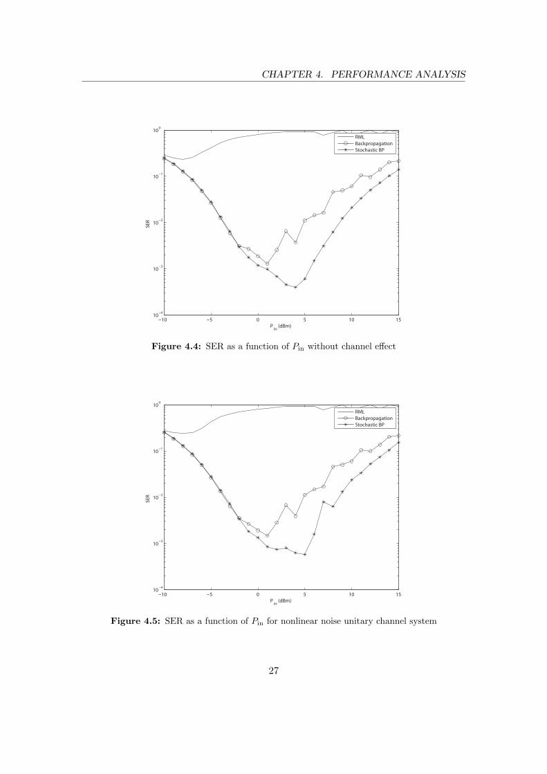
From Figure 4.4 we can tell that RML detector gives the worst performance, this ispredictable since it does not take SPM into account. The backpropagation detector ismuch better that RML, because its post-compensation of the phase shift. As the inputpower becomes bigger, the nonlinear phase noise effect increases while AWGN noiseeffect decreases. When SNR is low, the AWGN noise is the dominant component in thesystem, so the SER becomes lower when input power increases. When SNR is high,the nonlinear phase noise becomes the dominant components and cause the performancedegrades. The oscillation in the curve is caused by the interaction between linear noiseand SPM[1]. The stochastic backpropagation detector we provided in this thesis givesthe best performance of these three detector. It considers not only the nonlinearity butalso the linear noise interaction. The lowest SER we achieved is about 3.98×10−4, whenPin = 4 dBm.

The results with channel estimation by 1000 training symbols are shown in Fig-ure 4.5 We can find that the results of RML and backpropagation detector are almostsame as before, while the performance of stochastic backpropagation detector degraded.Especially when SNR is high, the SER of backpropagation detector increases very fast.However, the stochastic backpropagation detector still gives the lowest SER compare to

26


−10 −5 0 5 10 1510

−4

10−3

10−2

10−1

100

SE

R

Pin

(dBm)

RML

Backpropagation

Stochastic BP

Figure 4.4: SER as a function of Pin without channel effect

−10 −5 0 5 10 1510

−4

10−3

10−2

10−1

100

SE

R

Pin

(dBm)

RML

Backpropagation

Stochastic BP

Figure 4.5: SER as a function of Pin for nonlinear noise unitary channel system

27


other detector. The minimum value is 5.8× 10−4 when Pin = 5 dBm

4.2.2 Channel estimation results

As we discussed in the above section, the channel estimation method we provided inchapter 3 works very well in linear noise system, so the possible reason that the perfor-mance becomes worse is the nonlinear phase noise effect the channel estimation results.To verify this assumption,we simulate the channel estimation results. We fix the inputpower to 5.5 dBm, which gives the SER Ps = 9.2× 10−4 when there is no channel effect.We change the number of training symbols from 10 to 1000, calculate SER for thesevalues, the results is given in Figure 4.6.

0 200 400 600 800 1000 1200 140010

−3

10−2

10−1

100

SER

Number of training symbols

Figure 4.6: SER as a function of Nt

If we compare Figure 4.6 and Figure 4.3, we can find that the results are almostthe same, especially when Nt > 600, which means the channel estimation performanceis still good. So the real reason cause the detection performance degradation is thedetector is quite sensitive to the minor errors of channel estimation. Since we use thestochastic backpropagation method, the minor errors will be enlarged in every span,after transmitted through 22 spans, the errors are big enough to effect the detection.This effect is more obvious when nonlinear phase noise dominant the system, becausethe nonlinear phase noise is a deterministic function, so the error cannot be eliminate.That is why the SER decreases fast when SNR becomes bigger.

4.3 Linear non-unitary channel

We will discuss performances of the MMSE and ZF equalizers of two different channels.Besides the simulation results of different γ will also be mentioned.

28


4.3.1 simulation results

The following five figures show the simulation results of linear PDL channel. The com-munication system is set up with 22 fiber spans, the input power is from −10dB to 25dB,and the detector is the regular ML detector. Figure 4.7 shows the result for γ equals to0.99, the signal is dual polarization QPSK signal, the perfect knowledge of the channelis known and both ZF and MMSE equalizer are applied.

−10 −5 0 5 10 1510

−6

10−5

10−4

10−3

10−2

10−1

100

SE

R

Pin

(dB)

ZF

MMSE

AWGN

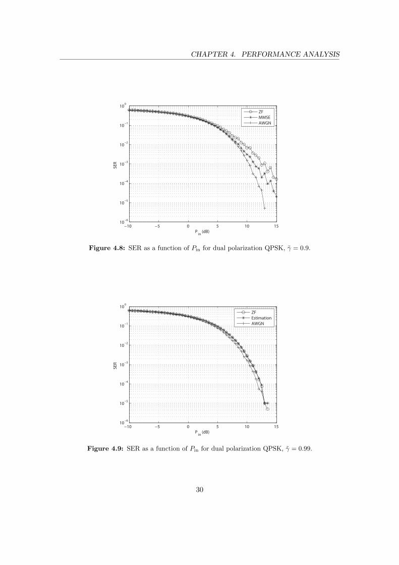
Figure 4.7: SER as a function of Pin for dual polarization QPSK, γ = 0.99.

Figure 4.8 shows the result for γ equals to 0.9, the signal is dual polarization QPSKsignal, the perfect knowledge of the channel is known and both ZF and MMSE equalizersare applied, but the channel is the noise-added first PDL channel which mentioned insection 3.2.

Figure 4.9 and Figure 4.10 show the results for γ equals to 0.99, the signal is dualpolarization QPSK signal, ZF and MMSE equalizers are applied individually with theestimation of the channel.

Figure 4.11 shows the result for γ equals to 0.99, the signal is dual polarization16-QAM signal, the perfect knowledge of the channel is unknown and ZF equalizer isapplied.

4.3.2 Performance analysis

Figure 4.7 and Figure 4.8 show the performances of ZF and MMSE equalizers of thetwo different channels, one is the channel we use, the other is a channel for comparison.Figure 4.7 shows that MMSE and ZF equalizers have the same performance. The atten-uation fact γ is 0.99, so comparing with the Figure 4.8 the AWGN curve is little higher,in Figure 4.7 to maintain SER of 10−3 the power we need is 10.16dB in Figure 4.8 is

29


−10 −5 0 5 10 1510

−6

10−5

10−4

10−3

10−2

10−1

100

SE

R

Pin

(dB)

ZF

MMSE

AWGN


−10 −5 0 5 10 1510

−6

10−5

10−4

10−3

10−2

10−1

100

SE

R

Pin

(dB)

ZF

Estimation

AWGN


30


−10 −5 0 5 10 1510

−6

10−5

10−4

10−3

10−2

10−1

100

SE

R

Pin

(dB)

MMSE

Estimation

AWGN


−10 −5 0 5 10 15 20 2510

−6

10−5

10−4

10−3

10−2

10−1

100

SE

R

Pin

(dB)

ZF

Estimation

AWGN

Figure 4.11: SER as a function of Pin for dual polarization 16-QAM, γ = 0.99.

31


10.39dB. In Figure 4.8 the MMSE equalizer has a much better performance than theZF equalizer, this is due to the noise as we have proved in the data detection section. Inboth these figures, the channel is known, the equalizer is built on the perfect knowledgeof the channel.

Figure 4.9 and Figure 4.10 show that on the same channel with the same estima-tion, the ZF equalizer and MMSE equalizer has nearly the same performance. In thesesituations, the channels are unknown.

Figure 4.11 shows the performance of ZF equalizer for 16-QAM signal. 16-QAMrequires more power to maintain low SER, as it is more sensitive to the channel losses,the points on the constellation are more dense than QPSK. The SER of 10−3 requiresinput power of 18dB. As the ZF equalizer and the MMSE equalizer has the sameperformance, in the estimation, ZF equalizer is used, as it is easier to fulfill.

4.4 Non-linear non-unitary channel

In this section, the modulation format is dual polarization 16-QAM.


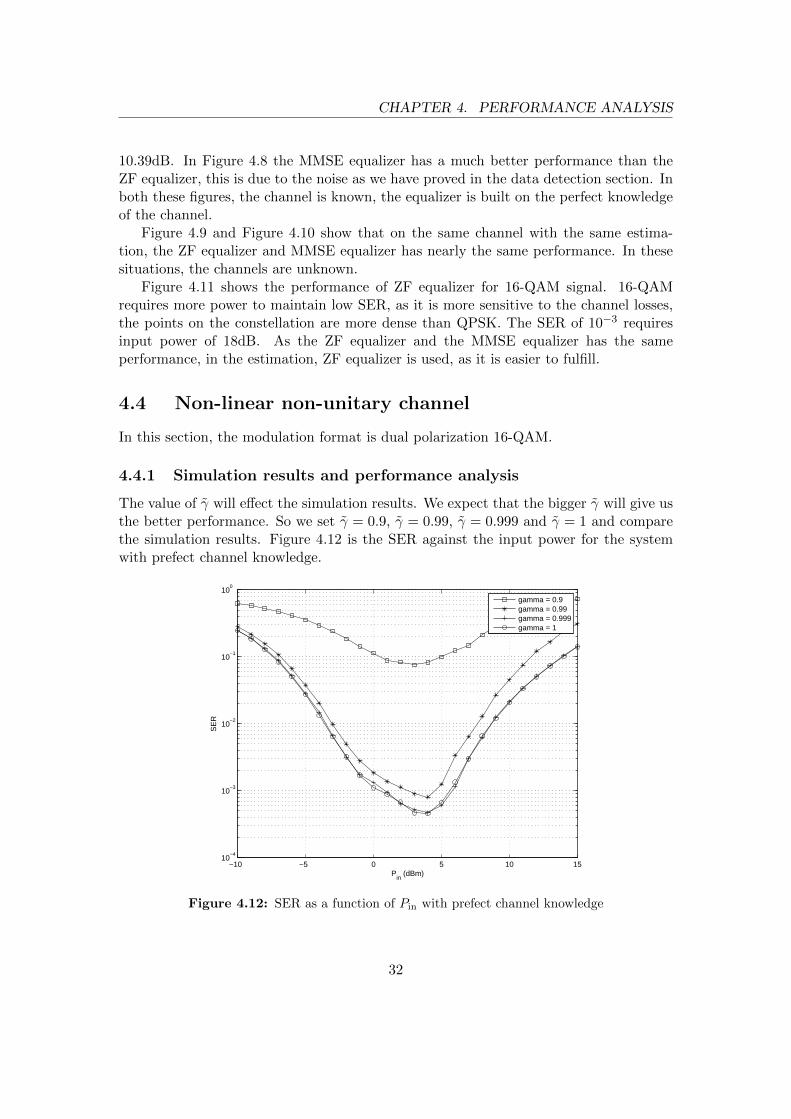
The value of γ will effect the simulation results. We expect that the bigger γ will give usthe better performance. So we set γ = 0.9, γ = 0.99, γ = 0.999 and γ = 1 and comparethe simulation results. Figure 4.12 is the SER against the input power for the systemwith prefect channel knowledge.

−10 −5 0 5 10 1510

−4

10−3

10−2

10−1

100

SE

R

Pin

(dBm)

gamma = 0.9gamma = 0.99gamma = 0.999gamma = 1

Figure 4.12: SER as a function of Pin with prefect channel knowledge

32


It is shown in the figure that our prediction is correct, when γ is bigger, the per-formance is obviously better. When γ = 0.9, the performance of the detector is reallybad, the lowest SER is 0.0757. When γ = 0.99, the lowest SER we reached is 8× 10−4

and when γ = 0.999 the lowest SER is 4.7× 10−4, the corresponding input power is −4dBm. When γ = 1, the lowest SER is 4.6× 10−4. Which means the performance of thedetector will not increase obviously after γ reaches 0.999. If we compare with the resultsfor nonlinear noise, unitary channel system, the results of nonlinear non-unitary systemis still acceptable when γ = 0.999.

33

5Conclusion

We provide a detector of coherent optical communication system with SPM and PDLchannel effect. The detection process contains two essential parts: channel estimationand data detection. To simplify the problem we also considered several transmissionmodel with different combination of noise and channel.

5.1 Unitary channel estimation

The estimation of unitary channel is based on the channel character and Monte Carlotechnique. We send training symbols to gain knowledge of the channel, use a simplemethod to calculate the estimation. As the results shows, the estimation method workswell for both linear and nonlinear noise environments. We also discussed about thenumber of training symbols and the results for perfect channel estimation.

5.2 Non-unitary channel estimation

The channel estimation is suitable for a memoryless channel with AWGN noise. Wehave also explained the reason that why the performance of the ZF equalizer and MMSEequalizer are the same. From the simulation, we can get a reasonable result of the SERagainst the input power.

5.3 Data detection with backpropagation

We use factor graph to analyze the system, use particle representation to collect informa-tion, use Monte Carlo method to generate stochastic distribution. We start our researchwith the traditional AWGN system and then extend our method to the communica-tion system with nonlinear phase noise and PDL channel effect. The backpropagationmethod gives better performance comparing to other detection method provided in this

34

CHAPTER 5. CONCLUSION

thesis when nonlinearity is considered and still has a good performance even we combinethe PDL channel effect.

35

6Future Work

In the previous sections, we have discussed the basic principle of backpropagation de-tector for a coherent optical communication system. In order to simplify the simulation,we neglect the effects such as intersymbol interference (ISI) and the noise introduced bythe components of the optical fiber. In the future work, such affects should be takeninto the consideration.

6.1 Channel estimation for nonlinear non-unitary system

In the last part of our thesis, we only provide the data detection method without channelestimation. In practical work, the channel information is unknown so an estimationmethod must be applied. Since the attenuation fact γ is easy to measure, the majorproblem is how to estimate the unitary channels in each span.

6.2 ISI

Intersymbol interference (ISI) is a kind of signal distortion, in which the signal interfereswith the subsequent signals. ISI add noise during the transmission, so the communicationwill be less reliable. ISI is usually caused by the multipath propagation and bandlimitedchannels. In this thesis, the ISI is mainly caused by the multipath propagation, as thedual polarization sends two different signals through the same fiber. The cause of thisis reflection. Since these paths have the different lengths, the signal will be delayed bythe reflection, and the baseband signal will spread to the sub-band. The phase of thereceived signal will be highly affected by these. In practice the ISI is also caused bydispersive effects such as Circular Dichroism (CD) and PMD.

The basic concept to prevent the ISI is adding the guard-band during the transmis-sion, but these will reduce the spectrum efficiency. Another ways to fight against ISI areapplying adaptive equalization and using error correcting codes. An adaptive equalizer is

36

CHAPTER 6. FUTURE WORK

an equalizer can adapt the properties of the time-varying of a channel. Error correctionis the correction and reconstruction of the original signal.

6.3 Other problems

As mentioned in the previous section, all the noise introduced by the components of thetransmission line were neglected. So in the future work, these noises should be added.For instance, the receiver noise, there are three basic sources of noises added to a receivedsignal, shot noise (photoelectron noise) which arises from the particle properties if thelight, thermal noise (circuit noise) which aries from the random movement of the electrondue to the temperature and optical noise (photon noise). All these will affect the resultsof the transmission.

37

Bibliography

[1] A. S. Tan, H. Wymeersch, P. Johannisson, E. Agrell, P. Andrekson, M. Karlsson,“An ML-based detector for optical communication in the presence of nonlinear phasenoise, ”International Conference on Communications (2010) .

[2] I. P. Kaminow, T. Li, A. E. Willner, “Coherent optical communicaion systems,”Optical fiber telecommunications 1 (5) (2010) 95.

[3] E. Ip, J. Kahn,“Compensation of dispersion and nonlinear impairments using digitalbackpropagation, ”Journal of Lightwave Technology 26 (20) (2008) 3416–3425.

[4] J. Gordon, L. Mollenauer, “Phase noise in photonic communications systems usinglinear amplifiers, ”Optics Letters 15 (23) (1990) 1351–1353.

[5] K. Ho, J. Kahn, “Electronic compensation technique to mitigate nonlinear phasenoise, ”Journal of Lightwave Technology 22 (3) (2004) 779–783.

[6] A. Lau, J. Kahn, “Signal design and detection in presence of nonlinear phase noise,”Journal of Lightwave Technology 25 (10) (2007) 3008–3016.

[7] H. Kim, A. Gnauck, “Experimental investigation of the performance limitation ofDPSK systems due to nonlinear phase noise, ”IEEE Photonics Technology Letters15 (320–322).

[8] L. Coelho, O. Gaete, E. Schmidt, B. Spinnler, N. Hanik, “Impact of PMD andnonlinear phase noise on the global optimization of DPSK and DQPSK systems,”Optical Fiber Communication Conference (OFC) (2010) OWE5.

[9] A. Technologies, “Polarization Dependent Loss Measurement of Passive OpticalComponents” (5988-1232EN) (2002) 3.URL http://cp.literature.agilent.com/litweb/pdf/5988-1232EN.pdf

[10] A. Technologies, “Measuring Polarization Dependent Loss of Passive Optical Com-ponents” (5990-3281EN) (2008) 2.URL http://cp.literature.agilent.com/litweb/pdf/5990-3281EN.pdf

38

http://cp.literature.agilent.com/litweb/pdf/5988-1232EN.pdf

http://cp.literature.agilent.com/litweb/pdf/5990-3281EN.pdf

BIBLIOGRAPHY

[11] Y. Cai, “MAP detection for linear and nonlinear ISI mitigation in long-haul coherentdetection systems, ”Photonics Society Summer Topical Meeting Series (2010) 42–43.

[12] X. Li, X. Chen, G. Goldfarb, E. Mateo, I. Kim, F. Yaman, G. Li, “Electronicpost-compensation of WDM transmission impairments using coherent detection anddigital signal processing, ”Opt. Expr. 16 (2) (2008) 881–888.

[13] W. Shieh, H. Bao, Y. Tang, “Coherent optical OFDM: Theory and design, ”Opt.Expr. 16 (2) (2008) 841–859.

[14] L. S. Muppirisetty, J. Karout, “Coherent optical OFDM: Theory and design (EX32)(2009) 43.

39

stochastic backpropagation for coherent optical communication

Documents