stochastic inverse problem with noisy simulator ... › ~klein › nabiltoulouse.pdf · stochastic...

STOCHASTIC INVERSE PROBLEM WITH NOISY

SIMULATOR

- APPLICATION TO AERONAUTICAL MODEL -

by

Nabil Rachdi, Jean-Claude Fort & Thierry Klein

Abstract. � Inverse problem is a current practice in engineering where the goal is toidentify parameters from observed data through numerical models. These numerical mod-els, also called Simulators, are built to represent the phenomenon making possible theinference. However, such representation can include some part of variability or commonlycalled uncertainty (see [3]), arising from some variables of the model. The phenomenon westudy is the fuel mass needed to link two given countries with a commercial aircraft, wherewe only consider the Cruise phase .From a data base of fuel mass consumptions during the cruise phase, we aim at identifyingthe Speci�c Fuel Consumption (SFC) in a robust way, given the uncertainty of the cruise

speed V and the lift-to-drag ratio F .In this paper, we present an estimation procedure based on Maximum-Likelihood estima-tion, taking into account this uncertainty.

Résumé. � Le problème inverse est une pratique assez courante en ingénierie, où lebut est de déterminer les causes d'un certain phénomène à partir d'observations de cedernier. Le phénomène mis en jeu est représenté par un modèle numérique, dont certainescomposantes peuvent comporter une part de variabilité (voir [3]). Le phénomène étudié estla masse de fuel nécessaire pour e�ectuer une liaison �xée avec un avion commercial, en neconsidérant que la phase de Croisière. Le but étant, à partir de données de masses de fuelconsommées en croisière, d'identi�er de manière robuste la consommation spéci�que SFCde la motorisation en tenant compte de l'incertitude sur la vitesse de croisière V et sur la�nesse F de l'avion.Dans cet article, nous proposons une procédure d'estimation basée sur une méthode demaximum de vraisemblance, prenant en compte cette incertitude.

Contents

1. Introduction. . . . . . . . . . . . . . . . . . . . . . . . . . . . . . . . . . . . . . . . . . . . . . . . . . . . . . . . . 22. General setting. . . . . . . . . . . . . . . . . . . . . . . . . . . . . . . . . . . . . . . . . . . . . . . . . . . . . . 23. Parameter estimation. . . . . . . . . . . . . . . . . . . . . . . . . . . . . . . . . . . . . . . . . . . . . . . . 64. Numerical study : �rst approach. . . . . . . . . . . . . . . . . . . . . . . . . . . . . . . . . . . . . 75. On the probabilistic modeling of SFC . . . . . . . . . . . . . . . . . . . . . . . . . . . . . . . 106. Theoretical result. . . . . . . . . . . . . . . . . . . . . . . . . . . . . . . . . . . . . . . . . . . . . . . . . . . . 16

Key words and phrases. � Inverse Problem, Uncertainty Analysis, Robust characterization,M-estimation.

We are grateful to Henri Yesilcimen for its contribution to the data generation and for fruitfuldiscussions.

2 NABIL RACHDI, JEAN-CLAUDE FORT & THIERRY KLEIN

7. Proof of Theorem 6.2. . . . . . . . . . . . . . . . . . . . . . . . . . . . . . . . . . . . . . . . . . . . . . . . 17References. . . . . . . . . . . . . . . . . . . . . . . . . . . . . . . . . . . . . . . . . . . . . . . . . . . . . . . . . . . . . 22

1. Introduction

One of engineering activities is to model real phenomena. Once a model is built (phys-ical principles, state equations, etc.), some parameters have to be identi�ed and somevariables of the model may present some intrinsic variability. Hence, the identi�cation ofparameters should implicitly take into account the uncertainty of variables of the model.In this paper, we present a likelihood-based method to estimate aeronautic parametersin a Fuel mass model. We use an analytical model that can be viewed as a black-boxsimulator. From a data baseM∗,1

fuel, ...,M∗,nfuel giving the mass of fuel consumed for n lines

between two given cities with a speci�c commercial aircraft, we aim at identifying theSpeci�c Fuel Consumption (SFC) which corresponds to a characteristic value of engines.The model we use depends in particular on the cruise speed (V ) and on the lift-to-dragratio (F ). These variables present intrinsic variability: the cruise speed may dependon atmospheric conditions and the lift-to-drag ratio is also subjected to variability po-tentially caused by turbulent phenomena. As a matter of fact, the identi�cation of theparameter SFC should take into account the variability of the cruise speed and thelift-to-drag ratio.In this paper, we propose an algorithm taken from the work of N. Rachdi et al. [5].It allows a characterization of SFC from the observed data M∗,1

fuel, ...,M∗,nfuel and model

simulations when the number of observations n is small.This article is organized as follows. In Section 2 we describe the setting of the problem.In Section 3 we build the algorithm for the inverse problem with a Maximum-Likelihoodbased method. In Section 4 we apply the algorithm given in Section 3. In Section 5 weillustrate the e�ect of modeling conditions, particularly the random modeling on SFCand the number of observed data. In Section 6 we establish the Theorem 6.2 providingan upper bound of the estimation error of the proposed algorithm. Section 7 is devotedto proving the Theorem 6.2.

2. General setting

2.1. Observations. � In our study, the data M∗,1fuel, ...,M

∗,nfuel were generated from an

aeronautic software which simulates gas turbine con�gurations used for power generation.In particular, it can simulate the consumed mass of fuel at some con�guration of engines,altitude, speed, atmospheric conditions, etc. (See Figure 1). This software is verycomplex and very much time consuming. In fact only 200 samples from this software areavailable by choosing various atmospheric conditions. This sample constitutes our datareference.In a �rst time, we pick up a small sample of size n = 32 from this reference sample.

The data are given in Table 1.Next, we will suppose that the observations M∗,1

fuel, ...,M∗,nfuel are drawn from an un-

known probability distribution Q with associated Lebesgue density f with support

I := [Minf = 7600,Msup = 8100] .

STOCHASTIC INVERSE PROBLEM IN AERONAUTICS 3

Figure 1. Aeronautic software

Reference Fuel Masses [kg]

7918 7671 7719 7839 7912 7963 7693 78157872 7679 8013 7935 7794 8045 7671 79857755 7658 7684 7658 7690 7700 7876 77698058 7710 7746 7698 7666 7749 7764 7667

Table 1. Simulated mass of fuel consumptions from aeronautic software

The di�erenceMsup−Minf = 500 kg have to be thought as an overconsumption of about7% approximatively.

2.2. A simplify aeronautic model. � We recall that we are interested in identi-fying the speci�c fuel consumption SFC. It is a signi�cant factor determining the fuele�ciency of a particular engine, with a small sample of "real" observations (here n = 32).To handle this problem we introduce a classical simpli�ed Fuel mass model given by theBréguet formula:

Mfuel = (Mempty +Mpload)(eSFC·g·Ra

V ·F 10−3 − 1).(1)

The �xed variables are

• Mempty : Empty weight = basic weight of the aircraft (excluding fuel and passengers),• Mpload : Payload = maximal carrying capacity of the aircraft,• g : Gravitational constant,• Ra : Range = distance traveled by the aircraft.

The uncertain variables mentioned in the introduction are

• V : Cruise speed = aircraft speed between ascent and descent phase,• F : Lift-to-drag ratio = aerodynamic coe�cient.

Table 2 gives the �xed variables values and the nominal values considered for uncertainvariables.

2.3. Noise modeling. � As said in the introduction, we have to take into accountthe uncertainty of the cruise speed V and the lift-to-drag ratio F . Given the nominalvalue of each variable (see Table 2), an expert judgment can derive the uncertaintybounds. (see Table 3).The uncertainty on the cruise speed V represents a relative di�erence of arrival time

of 8 minutes.


input value or nominal value unit

Mempty 42600 kgMpload 19900 kgg 9.8 m/s2

Ra 3000 kmVnom 231 m/sFnom 19 �

Table 2. Values of Fuel mass model inputs

variable nominal value min max

V 231 226 234F 19 18.7 19.05

Table 3. Minimal and maximal values of uncertain variables

Moreover, specialists in turbine engineering propose to model the uncertainties as pre-sented in Table 4.

variable distribution parameter

V Uniform (Vmin, Vmax)F Beta (7, 2, Fmin, Fmax)Table 4. Uncertainty modeling

The probability density function of a beta distribution on [a, b] with shape parameters(α, β) is

g(α,β,a,b)(x) =(x− a)(α−1)(b− x)β−1

(b− a)β−1B(α, β)1 [a,b](x) ,

where B(·, ·) is the beta function.Figure 2 shows the probability density functions of V and F .

18.80 18.85 18.90 18.95 19.00 19.05 19.10 19.15

02

46

8

Uncertainty on the lift−to−drag ratio

x

PD

F

Uncertainty on F

(a)

225 230 235

0.00

0.05

0.10

0.15

Uncertainty on the cruise speed

x

PD

F

Uncertainty on V

(b)

Figure 2. (a) Uncertainty on F . (b) Uncertainty on V .

In order to emphasize the "noisy" feature of the variables V and F , we will use thewriting


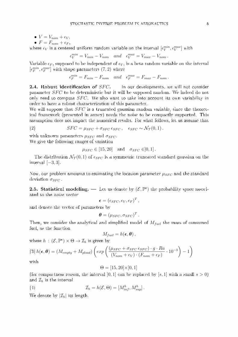
• V = Vnom + εV ,• F = Fnom + εF ,

where εV is a centered uniform random variable on the interval [εminV , εmaxV ] with

εminV = Vmin − Vnom and εmaxV = Vmax − Vnom .Variable εF , supposed to be independent of εV , is a beta random variable on the interval[εminF , εmaxF ] with shape parameters (7, 2) where

εminF = Fmin − Fnom and εmaxF = Fmax − Fnom .

2.4. Robust identi�cation of SFC. � In our developments, we will not considerparameter SFC to be deterministic but it will be supposed random. We indeed do notonly need to compute SFC. We also want to take into account its own variability inorder to have a robust characterization of this parameter.We will suppose that SFC is a truncated gaussian random variable, since the theoret-ical framework (presented in annex) needs the noise to be compactly supported. Thisassumption does not impact the numerical results. For what follows, let us assume that

SFC = µSFC + σSFC εSFC , εSFC ∼ NT (0, 1) .(2)

with unknown parameters µSFC and σSFC .We give the following ranges of variation

µSFC ∈ [15, 20] and σSFC ∈]0, 1] .

The distribution NT (0, 1) of εSFC is a symmetric truncated standard gaussian on theinterval [−3, 3].

Now, our problem amounts to estimating the location parameter µSFC and the standarddeviation σSFC .

2.5. Statistical modeling. � Let us denote by (E ,Pε) the probability space associ-ated to the noise vector

ε = (εSFC , εV , εF )T ,

and denote the vector of parameters by

θ = (µSFC , σSFC)T .

Then, we consider the analytical and simpli�ed model of Mfuel the mass of consumedfuel, as the function

Mfuel = h(ε,θ) ,

where h : (E ,Pε)×Θ→ Ih is given by

h(ε,θ) = (Mempty +Mpload)

(exp

((µSFC + σSFC εSFC) · g ·Ra(Vnom + εV ) · (Fnom + εF )

· 10−3

)− 1

)(3)

withΘ = [15, 20]×]0, 1]

(for compactness reason, the interval ]0, 1] can be replaced by [s, 1] with a small s > 0)and Ih is the interval

Ih = h(E ,Θ) = [Mhinf ,M

hsup] .(4)

We denote by |Ih| its length.


Remark 2.1. � We observe through simulations that

I ⊂ Ih ,where I = [Minf ,Msup] is the observation interval given above.

The purpose is now to estimate parameter θ ∈ Θ from the set of data M∗,1fuel, ...,M

∗,nfuel.

In the next section, we propose an estimation procedure taken from [5].

3. Parameter estimation

In our previous framework it is possible to apply the procedures developed in [5].In particular, we choose to work with the log−contrast which can be understood as aMaximum Likelihood based estimation.

The sample M∗,1fuel, ...,M

∗,nfuel is drawn from an unknown distribution Q. We will use the

parametric family of distributions {Qθ , θ ∈ Θ} where Qθ is the pushforward measure ofPε by the (measurable) application u 7→ h(u,θ) .That means that we consider the models h(ε, θ) to be a reasonable �rst approximationin order to obtain statistical information about Q.Denoting ρθ the Lebesgue density associated to the measure Qθ, the maximum likelihoodprocedure is given by

θ = Argminθ∈Θ

− 1

n

n∑i=1

log(ρθ(M∗,ifuel)) .(5)

However, the above procedure is unfeasible because the density ρθ is not analyticallytractable. As suggested in [5], we replace ρθ by an estimator denoted ρmθ . There aremany ways to estimate a density. We choose the simplest one, which is commonly usedin industrial modeling.

Let ε1, ..., εm be m random variables i.i.d from Pε, we consider the kernel estimate of ourdensity

ρmθ (·) =1

m

m∑j=1

Kbmθ(· − h(εj,θ)) ,(6)

where Kbmθis the gaussian kernel

Kbmθ(x) =

1√2π bmθ

e− x2

2 (bmθ

)2 ,

and bmθ is computed from the sample h(εj,θ), j = 1, ...,m for θ ∈ Θ, by Silverman'srule-of-thumb :

bmθ =

(4

3

)1/5

m−1/5 σθ .(7)

The quantity σθ is the empirical standard deviation of the sample h(εj,θ), j = 1, ...,m

σθ =1

m

m∑j=1

(h(εj,θ)− 1

m

m∑j=1

h(εj,θ)

)2

.


Other popular estimates are truncated projections on a suitable basis of functions(sine, cosine, wavelets, etc.). Here we do not discuss the optimization of the densityestimation, but all what follows could be applied in the same way. The numerical resultsmay be slightly di�erent, but qualitatively the same.Replacing ρθ by ρmθ in (5) and simplifying by the multiplying constant 1/n yields theestimation procedure

θ = Argminθ∈Θ

−n∑i=1

log

(1

m

m∑j=1

Kbmθ

(h(εj,θ)−M∗,i

fuel

)).(8)

Hence, our problem is an inverse problem. More precisely, it is an inverse problem inpresence of uncertainties, also called probabilistic inverse problem or stochastic inverseproblem. This topic is often treated in the �eld of uncertainty management: the goalmay for instance be to identify the intrinsic uncertainty of a system. A reference isthe work of E. de Rocquigny and S. Cambier [2] (and associated references), where thepurpose is to identify a parameter of interest which controls the vibration ampli�cationof stream turbines. Our framework is di�erent. The main di�erence lies in the absence ofassumptions, in the present paper, on the distribution of the error between observationdata and reference data. Thus, it di�erentiates the estimation procedures we proposefrom the ones developed in [2].

In the following section, we provide a numerical analysis using the algorithm given by(8). Theoretical aspects will be addressed in Section 6.

4. Numerical study : �rst approach

4.1. Estimation. � Setting

J(θ) = −n∑i=1

log

(1

m

m∑j=1

Kbmθ

(h(εj,θ)−M∗,i

fuel

))with θ = (µSFC , σSFC)T ,

our problem is a minimization problem where we want to compute

θ = Argminθ∈Θ

J(θ) .

We recall that n = 32. The data (M∗,ifuel)i=1,...,n are provided by Table 1. We choose

m = 10000 (the number of calls to the model given by (3)), and for j = 1, ...,m, εj ∼ Pε

where

Pε(du, dv, dw) =1√

2π Le−u

2/2 g(7,2,εminF ,εmaxF )(v)1

εmaxV − εminV

1 [εminV ,εmaxV ](w) du dv dw ,

with L = Φ(3)−Φ(−3) (Φ is the cumulative distribution function of a standard gaussianrandom variable).This optimization procedure can be solved by Quasi-Newton methods. We present theresults in Table 5. In Figure 3 we show the resulting probability density function of SFC

estimator value of J(θ) estimated SFC location estimated SFC dispersion

θ J(θ) = 199.465 µSFC = 17.397 σSFC = 0.201Table 5. SFC characterization parameters


given by NT (µSFC , σSFC) .

Figure 3. Estimated Speci�c Fuel Consumption distribution.

Figure 4 provides pro�le views of the criterion function θ = (µSFC , σSFC) 7→ J(θ),�rst at σSFC = σSFC (Figure 4(a), we show log(J(θ))) and then at µSFC = µSFC (Figure4(b)).

We notice that the minimum θ = (µSFC , σSFC) is correctly located.

(a) (b)

Figure 4. (a) Pro�le view of log(J) at σSFC = σSFC . (b) Pro�le view of J atµSFC = µSFC .

4.2. Comparison with reference sample. � In order to analyse the results ob-tained in the previous subsection, we need some reference sample of SFC values at thesame simulation conditions. We take for reference the sample of SFC values of size 200described in the introduction, provided by the aeronautic software. The characteristicsof this sample are given in Table 6.


Mean Stand. dev.

Reference sample 17.49 0.57Table 6. Reference sample characteristics

The data in Table 6 have to be compared with those in Table 5 where the mean andstandard deviation are µSFC = 17.397 and σSFC = 0.201, respectively. Table 7 providesthe associated relative errors. Figure 5 shows the histogram of the reference sample andthe estimated distribution of SFC obtained in Figure 3.

Reference sample Estimated SFC (3) Relative error

Mean 17.49 17.397 0.5 %Stand. dev. 0.57 0.201 60.6 %

Table 7. Relative errors of the mean and deviation between reference SFCsample and the estimated model (3)

Figure 5. Reference and estimated SFC distributions.

It appears that the location of the variable of interest SFC is well reached whereas thestandard deviation estimation provides an error of 60%. The "error" has roughly twoorigins:

Statistical error: : this error is mainly due to the limited number (n = 32) of datafrom the observed masses of fuel M∗,i

fuel. It is also due to the error induced by thekernel approximation of ρθ.Yet the choice ofm = 10000 calls to the analytical modelgarantees that the error on ρθ is small .


Model error: : this error is relative to the use of Fuel mass model (1) with uncertainvariables V and F (Figure 2), and includes the gaussian hypothesis for SFC (2).Thus, the model error can be separated into 2 parts: physical model error anduncertainty modeling error.

We observe on Figure 5 that the SFC parameter does not behave like a gaussianvariable. This can be quali�ed as model error.However, if one just wants to estimate the mean value of SFC, the gaussian hypothesisdoes not have a signi�cative impact (0.5% of error). On the other hand, if one wantsmore information about SFC, other modeling tools are needed to allow a robustcharacterization approach.

In the next subsection, we will discuss the uncertainty modeling, more precisely, thegaussian hypothesis for SFC given by (2).

5. On the probabilistic modeling of SFC

5.1. Considering Wiener-Hermite representation in the previous analysis. �The characterization of a random variable by the mean and the standard deviation onlycould be too approximative in order to study the whole behavior of the variable. In thisstudy, we have made an a priori (a model) on the variable of interest SFC. In (2) wesupposed that

SFC ∼ NT (µSFC , σ2SFC) ,

which we now rewrite

SFC = µSFC + σSFC ξT , ξT ∼ NT (0, 1) .(9)

We will see that this gaussian hypothesis on SFC is a particular case of a more generalrepresentation.

The so called Wiener Chaos Expansion, developed in the 30's by Wiener [9], gives arepresentation of any second-order random variable Z:

Z =∞∑l=0

zlΥl((ξk)k≥1) , (with convergence in L2(P) )(10)

where (ξk)k≥1 is a (in�nite) sequence of independent standard normal random variablesand the Υl's are the multivariate Hermite polynomials. This expansion is also calledWiener-Hermite expansion.In practice, we have to consider a �nite sequence (ξ1, ..., ξM) where M is called theorder of the expansion, and the sum in (10) is truncated at p which is the degree of theexpansion.Hence, considering all M -dimensional Hermite polynomials of degree lower than p, therepresentation (10) is approximated by

Z ' Zp,M =P−1∑l=0

zlΥl(ξ) , ξ = (ξ1, ..., ξM) ,(11)

where

P =(M + p)!

M ! p!.


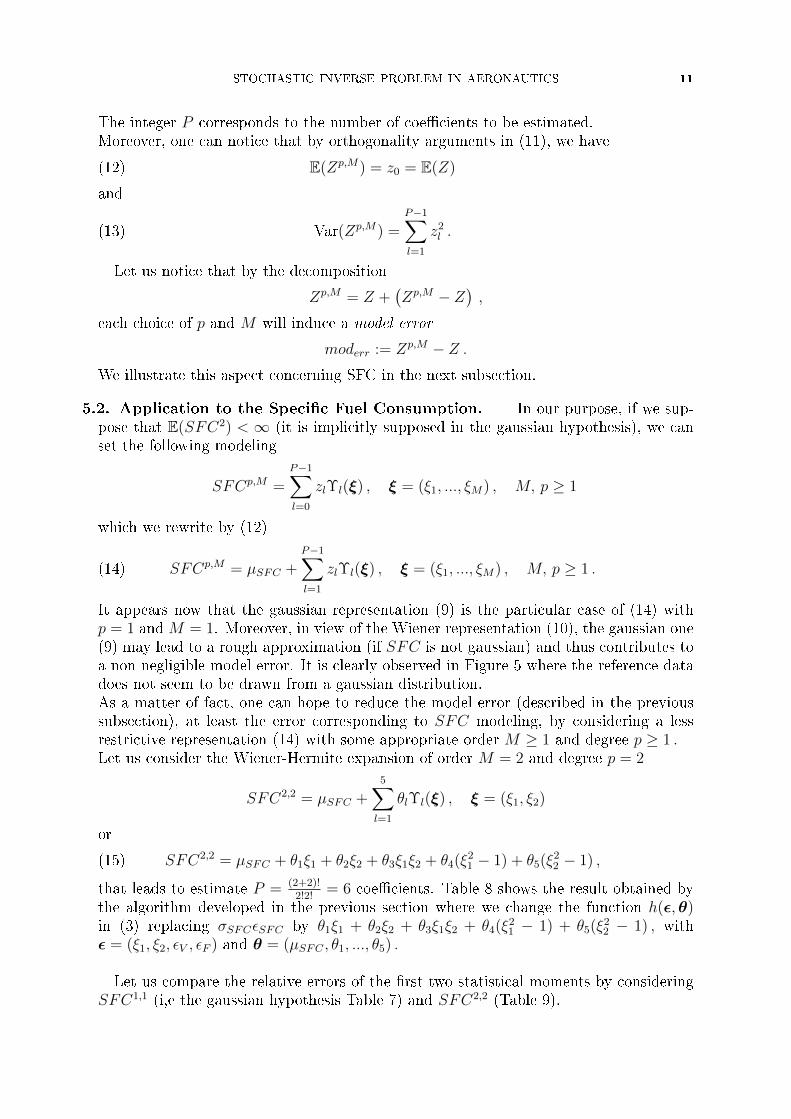
The integer P corresponds to the number of coe�cients to be estimated.Moreover, one can notice that by orthogonality arguments in (11), we have

E(Zp,M) = z0 = E(Z)(12)

and

Var(Zp,M) =P−1∑l=1

z2l .(13)

Let us notice that by the decomposition

Zp,M = Z +(Zp,M − Z

),

each choice of p and M will induce a model error

moderr := Zp,M − Z .We illustrate this aspect concerning SFC in the next subsection.

5.2. Application to the Speci�c Fuel Consumption. � In our purpose, if we sup-pose that E(SFC2) < ∞ (it is implicitly supposed in the gaussian hypothesis), we canset the following modeling

SFCp,M =P−1∑l=0

zlΥl(ξ) , ξ = (ξ1, ..., ξM) , M, p ≥ 1

which we rewrite by (12)

SFCp,M = µSFC +P−1∑l=1

zlΥl(ξ) , ξ = (ξ1, ..., ξM) , M, p ≥ 1 .(14)

It appears now that the gaussian representation (9) is the particular case of (14) withp = 1 andM = 1. Moreover, in view of the Wiener representation (10), the gaussian one(9) may lead to a rough approximation (if SFC is not gaussian) and thus contributes toa non negligible model error. It is clearly observed in Figure 5 where the reference datadoes not seem to be drawn from a gaussian distribution.As a matter of fact, one can hope to reduce the model error (described in the previoussubsection), at least the error corresponding to SFC modeling, by considering a lessrestrictive representation (14) with some appropriate order M ≥ 1 and degree p ≥ 1 .Let us consider the Wiener-Hermite expansion of order M = 2 and degree p = 2

SFC2,2 = µSFC +5∑l=1

θlΥl(ξ) , ξ = (ξ1, ξ2)

or

SFC2,2 = µSFC + θ1ξ1 + θ2ξ2 + θ3ξ1ξ2 + θ4(ξ21 − 1) + θ5(ξ2

2 − 1) ,(15)

that leads to estimate P = (2+2)!2!2!

= 6 coe�cients. Table 8 shows the result obtained bythe algorithm developed in the previous section where we change the function h(ε,θ)in (3) replacing σSFCεSFC by θ1ξ1 + θ2ξ2 + θ3ξ1ξ2 + θ4(ξ2

1 − 1) + θ5(ξ22 − 1) , with

ε = (ξ1, ξ2, εV , εF ) and θ = (µSFC , θ1, ..., θ5) .

Let us compare the relative errors of the �rst two statistical moments by consideringSFC1,1 (i,e the gaussian hypothesis Table 7) and SFC2,2 (Table 9).


θ0 θ1 θ2 θ3 θ4 θ5

SFC2,2 17.470 0.047 0.054 0.182 0.103 0.063Table 8. SFC characterization parameters

Reference sample from SFC2,2 Relative error

Mean 17.49 17.470 0.11 %Stand. dev. 0.57 0.230 59.65 %

Table 9. Relative errors of the mean and standard deviation with SFC2,2

The Wiener-Hermite modeling seems to improve the mean estimation of SFC whereasthe standard deviation is poorly estimated in the two cases with an error of about60%. There is no signi�cative di�erence between the two methods regarding the �rsttwo moments. However, the behavior of density functions corresponding to SFC1,1 (seeFigure 5) and SFC2,2 is clearly not the same. We present in Figure 6 the result obtainedwhen SFC is modeled by a Wiener expansion of order M = 2 and degree p = 2.

Figure 6. Estimations of SFC probability density with a Wiener Expansionp =M = 2 .

The distribution of SFC given by the Wiener expansion in Figure 6 seems to havea behavior close to the reference sample one, despite the fact that there is a nonnegligible bias. As mentioned in the previous subsection, this is due to the statisticaland model errors. Indeed, let us recall that we have at disposal n = 32 reference fuelmasses from which we characterize the SFC parameter. It would be interesting to


see what happens when adding reference fuel masses, i.e by reducing the statistical error.

5.3. Wiener-Hermite analysis with augmented reference fuel mass sample.� We present here numerical results obtained by adding 50 new samples from the databasis built with the complex software with the same initial conditions. Figure 7 showsthe characterization of SFC obtained by a Wiener expansion of orderM = 2 and degreep = 2 from the augmented reference fuel mass sample of size n = 82.

Figure 7. Characterization of SFC with an augmented sample of fuel mass

The Table 10 gives the coe�cients corresponding to this simulation.

θ0 θ1 θ2 θ3 θ4 θ5

SFC2,2 17.50 0.281 0.008 0.012 0.191 0.219Table 10. SFC characterization parameters from augmented fuel mass sample

Hence, by adding reference data we improve signi�catively the characterization ofSFC on the �rst two statistical moments as well as on the whole probability densityfunction of SFC.

In the next section we introduce some knowledge on the SFC modeling through anexpert judgment inducing a new and statistical modeling that will improve to be better.


Reference sample from SFC2,2 Relative error

Mean 17.49 17.50 0.06 %Stand. dev. 0.57 0.404 29.12 %

Table 11. Relative errors of the mean and standard deviation with SFC2,2

from augmented fuel mass sample

5.4. Analysis with a "good" a priori knowledge. � In the previous analyses, weonly consider truncated Wiener-Hermite expansions. This is more of a mathematicalhypothesis than a knowledge brought to the modeling. Suppose now that an expertjudgment says that the distribution of the SFC is of exponential form. Mathematically,it is equivalent to supposing that the probability density of SFC belongs to the family{

p(u;θ) = θ2 e−θ2(u−θ1) 1 [θ1,+∞[ , θ = (θ1, θ2) ∈ R+ × R∗+

}.

One can check that this suggestion induces the modeling

SFCexp = θ1 −1

θ2

log(ξ) , ξ ∼ U([0, 1]) ,(16)

where U([0, 1]) is the uniform distribution on the interval [0, 1] .

Remark 5.1. � Representation (16) seems quite di�erent from the one provided bythe Wiener-Hermite expansions (see (9) and (15)). Yet, as the random variable SFCexp

has �nite variance, the modeling (16) could be seen as a practical alternative to a Wienerexpansion (10). Such a Wiener expansion would be given by choosing a high order M exp

and a high degree pexp in (11).

In what follows, we present the results of the numerical analysis corresponding ton = 32 and n = 82.

For n = 32,

θ1 θ2

SFCexp 17.23 3.45Table 12. Estimation of θ = (θ1, θ2) when n = 32

Reference sample from SFCexp (n = 32) Relative error

Mean 17.49 17.52 0.17 %Stand. dev. 0.57 0.29 49.12 %

Table 13. Relative errors of the mean and standard deviation between referenceSFC sample and SFCexp when n = 32.

For n = 82,We clearly see that the informative knowledge contributes to improving signi�catively

the characterization of the Speci�c Fuel Consumption. With n = 82 fuel mass data, theresults are satisfying as shown in Figure 8 and Table 15.


θ1 θ2

SFCexp 16.95 2Table 14. Estimation of θ = (θ1, θ2) when n = 82

Reference sample from SFCexp (n = 82) Relative error

Mean 17.49 17.45 0.23 %Stand. dev. 0.57 0.501 12.1 %

Table 15. Relative errors of the mean and standard deviation between referenceSFC sample and SFCexp when n = 82.

Figure 8. Characterization of SFC with an exponential hypothesis

5.5. Conclusion. � Section 5 was dedicated to illustrating the e�ect of the modelingconditions for SFC characterization. In particular, we showed the impact of a "modelerror" through the modeling of the random variable SFC. We also illustrated how thestatistical error, through the number of fuel mass data, appears in the performance ofthe estimation.In all cases, we computed a parameter θ. If we supposed that there is no model error,that is Q ∈ {Qθ, θ ∈ Θ}, the error is only due to the limited number of data. So it makes

sense to investigate the di�erence ‖θ − θ∗‖, where Q = Qθ∗ . If this is not the case itgives an insight on the statistical error part.It is the topic of the following section.


6. Theoretical result

In this paper, the study of the procedure performance (8) will be non-asymptotic, i.efor a �xed number of observations M∗,i

fuel (n) and a �xed number of variables εj (m).The asymptotic study is let to a forthcoming work.

The quality of such estimation procedure can be investigated by giving an upper bound

of the distance between the reachable parameter θ and the best parameter θ∗ (unknown).The latter can be seen as the parameter obtained if one has an in�nite number of obser-vations M∗,i

fuel and variables εj. More precisely,

θ∗ = Argminθ∈Θ

EQ log(ρθ(M∗

fuel)),(17)

where EQ log(ρθ(M∗

fuel))can be seen as the "limit" of the quantity

1

n

n∑i=1

log

(1

m

m∑j=1

Kbmθ

(h(εj,θ)−M∗,i

fuel

))(18)

in (8) when n and m go to in�nity.The Maximum Likelihood equation (17) turns out to be the minimization of theKullback-Leibler divergence between Q and the family {Qθ, θ ∈ Θ}, while equation (18)is a smoothed empirical counterpart.We consider the model h(ε,θ) given in (3), but what follows can be generalized to any

other one.Then, denoting by ‖ · ‖ the Euclidian norm in R2, it makes sense to bound the quantity

‖θ − θ∗‖2 .

Let us denote byR(θ) := EQ log

(ρθ(M∗

fuel)),

and by f the Lebesgue density associated to the measure Q .

Assumptions 6.1. � Let us consider the following assumptions.- A1 The map θ 7→ R(θ) is twice di�erentiable with

∇R(θ∗) = 0

and has a symmetric positive de�nite Hessian matrix ∇2R . Let us denote by λmin >0 the smallest eigenvalue of the set of matrices {∇2R(θ), θ ∈ Θ} .

- A2 It exists η > 0 such that for all θ ∈ Θ, the density probability of h(ε,θ) wenoted ρθ, satis�es

ρθ > η .

- A3 For all θ ∈ Θ, the second derivative of ρθ, we note ρ′′

θ, exists and

C := supθ∈Θ‖ρ′′θ‖2 < +∞ .

- A4 We suppose that

0 < δ < infθ∈Θ

σθ and supθ∈Θ

σθ < σ < +∞ ,

where σθ is de�ned in (7).

We prove the following consistency theorem:


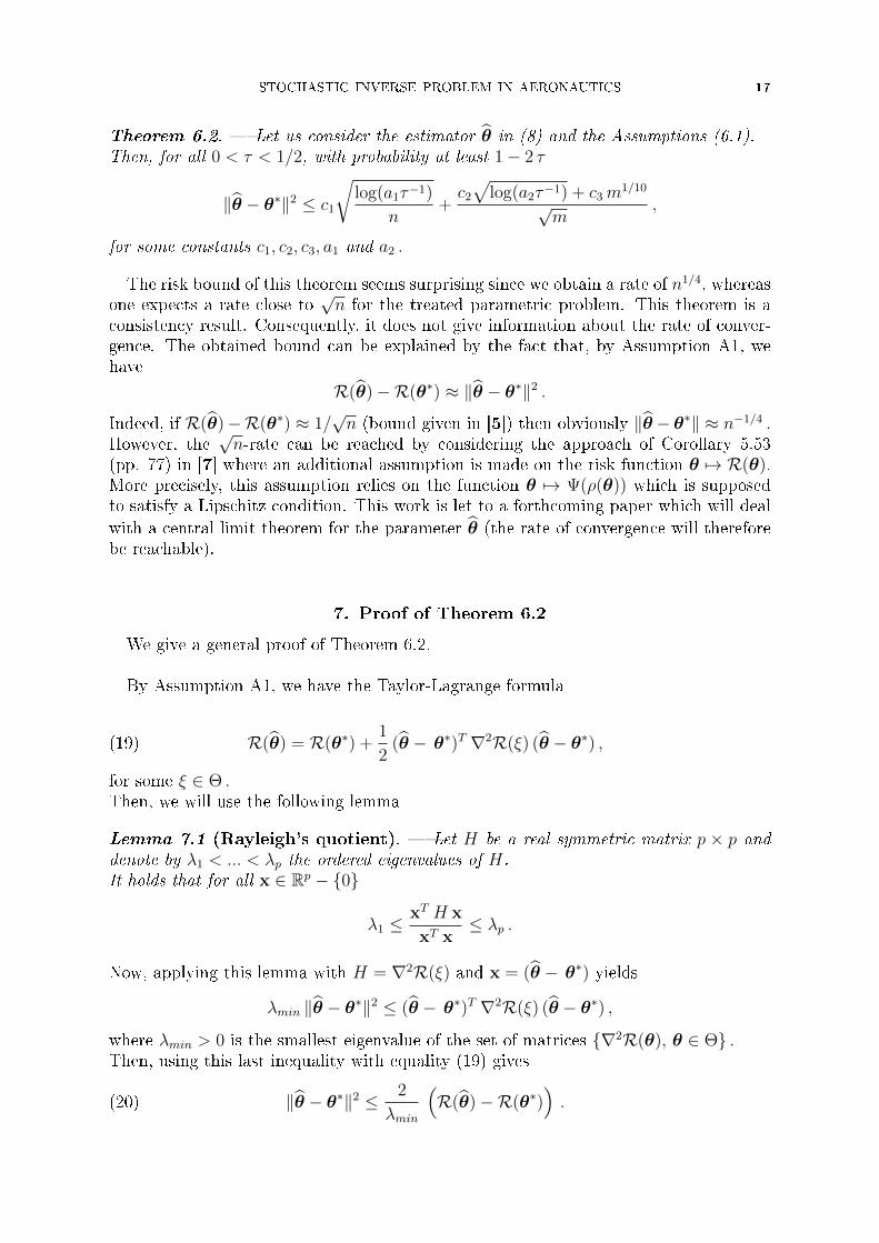
Theorem 6.2. � Let us consider the estimator θ in (8) and the Assumptions (6.1).Then, for all 0 < τ < 1/2, with probability at least 1− 2 τ

‖θ − θ∗‖2 ≤ c1

√log(a1τ−1)

n+c2

√log(a2τ−1) + c3m

1/10

√m

,

for some constants c1, c2, c3, a1 and a2 .

The risk bound of this theorem seems surprising since we obtain a rate of n1/4, whereasone expects a rate close to

√n for the treated parametric problem. This theorem is a

consistency result. Consequently, it does not give information about the rate of conver-gence. The obtained bound can be explained by the fact that, by Assumption A1, wehave

R(θ)−R(θ∗) ≈ ‖θ − θ∗‖2 .

Indeed, if R(θ)−R(θ∗) ≈ 1/√n (bound given in [5]) then obviously ‖θ− θ∗‖ ≈ n−1/4 .

However, the√n-rate can be reached by considering the approach of Corollary 5.53

(pp. 77) in [7] where an additional assumption is made on the risk function θ 7→ R(θ).More precisely, this assumption relies on the function θ 7→ Ψ(ρ(θ)) which is supposedto satisfy a Lipschitz condition. This work is let to a forthcoming paper which will deal

with a central limit theorem for the parameter θ (the rate of convergence will thereforebe reachable).

7. Proof of Theorem 6.2

We give a general proof of Theorem 6.2.

By Assumption A1, we have the Taylor-Lagrange formula

R(θ) = R(θ∗) +1

2(θ − θ∗)T ∇2R(ξ) (θ − θ∗) ,(19)

for some ξ ∈ Θ .Then, we will use the following lemma

Lemma 7.1 (Rayleigh's quotient). � Let H be a real symmetric matrix p × p anddenote by λ1 < ... < λp the ordered eigenvalues of H.It holds that for all x ∈ Rp − {0}

λ1 ≤xT H x

xT x≤ λp .

Now, applying this lemma with H = ∇2R(ξ) and x = (θ − θ∗) yields

λmin ‖θ − θ∗‖2 ≤ (θ − θ∗)T ∇2R(ξ) (θ − θ∗) ,

where λmin > 0 is the smallest eigenvalue of the set of matrices {∇2R(θ), θ ∈ Θ} .Then, using this last inequality with equality (19) gives

‖θ − θ∗‖2 ≤ 2

λmin

(R(θ)−R(θ∗)

).(20)


The problem turns to bound the positive quantity R(θ)−R(θ∗), where θ is given by(8). Such bound can be investigated by applying Theorem 4.1 in [5], which is a generalresult. We will aim at computing constants Kτ

1 and Kτ2 such that, with high probability

(21)

R(θ)−R(θ∗) ≤ 2 ‖f‖2

η

(1√n

η

2 δ2 ‖f‖2

γ Kτ1 +

1√m

1√2π δ

Kτ2 +

1

m2/5

C (1.06σ)2

√3

).

In our framework, the main work is to compute the concentration constants Kτ1 and Kτ

2

derived from [5] in the following particular case.

7.1. On concentration constants Kτ1 and Kτ

2 . � First of all, let us recall somede�nitions and notations relative to empirical processes.

De�nition 7.2. � Empirical process. Let W be some probability measure on somespace T and let us suppose given a k i.i.d sample ξ1, ..., ξk drawn from W . Let us denoteby Wk the empirical measure

Wk :=1

k

k∑i=1

δξi

and G some class of real valued functions g : T → R .We call W -empirical process indexed by G the following application

Gk : G −→ R

g 7−→ Gk :=√k

∫T

g(t) (Wk −W ) (dt) ,

also written

Gk g :=1√k

k∑i=1

(g(ξk)− EW (g(ξ))) .

We denote the supremum of an empirical process by

‖Gk‖G := supg∈G|Gk g| .

Following the proof lines of Theorem 2.1, Table 2 p.11 in [5] (giving classes of functions)and considering the inequality (21), it is easy to verify that Kτ

1 is de�ned as

for all n ≥ 1 , P(‖Un‖A ≤ Kτ1 ) ≥ 1− τ(22)

where Un is the Q-empirical process (Qn = 1n

∑ni=1 δM∗,ifuel

) indexed by the class of func-

tions

A = {y ∈ I 7−→ (y − λ)2, λ ∈ Ih}(23)

where we recallI = [Minf ,Msup] and Ih = h(E ,Θ) .

Similarly, the constant Kτ2 is de�ned as follows

for all m ≥ 1 , P(‖Vm‖B ≤ Kτ2 ) ≥ 1− τ(24)

where Vm is the P ε-empirical process (P εm = 1

m

∑mj=1 δεj) indexed by the class of functions

B = {x ∈ E 7−→ e−(h(x,θ)−λ)2/2 b2 , (θ, λ, b) ∈ Θ× Ih × [δ, σ]} .(25)


By the writings (22) and (24), the constants Kτ1 and Kτ

2 arise from the "concentration ofthe measure phenomenon" (see [4], [1]). More precisely, these constants characterize thetightness of the sequences of random variables ‖Un‖A (which is (M∗,i

fuel)i=1,...,n dependent)and ‖Vm‖B (which is (εj)j=1,...,m dependent).

Now, we aim at computing (upper bound) these constants using concentration inequali-ties where the classes of functions A and B will play a crucial role. In particular, we willapply the following theorem which is Theorem 2.14.9 in [8].Before, let us recall the de�nition of the bracketing numbers (taken from [8] p. 83-85).

De�nition 7.3. � Bracketing numbers. Let G be some class of functions on T anddenote by W a probability measure on T .Given two functions l, u, the bracket [l, u] is the set of all functions g with l ≤ g ≤ u. Anε-bracket is a bracket [l, u] with ||u−l||2,W < ε. The bracketing number N[ ](ε, G, L2(W ))is the minimum number of ε-brackets needed to cover the class of functions G.The entropy with bracketing is the logarithm of the bracketing number.

Remark 7.4. � The bracketing numbers measure the "size", the complexity of a classof functions.

Theorem 7.5. � Let G be a uniformly bounded class of (measurable) functions g :T → [0, 1] and denote by W a probability measure on T . If the class G satis�es, for someconstants K and L

N[ ](ε,G, L2(W )) ≤(K

ε

)Lfor every 0 < ε < K .(26)

Then, for every t > 0,

P(‖Gk‖G > t) ≤(D t√L

)Le−2t2 ,

for a constant D that only depends on K.

The proof of this theorem can be found in [6].

Now, let Kτ be a constant (to determine) which satis�es

P(‖Gk‖G ≤ Kτ ) ≥ 1− τ .This is equivalent to

P(‖Gk‖G > Kτ ) ≤ τ .(27)

By Theorem 7.5, applied with t = Kτ , we have

P(‖Gk‖G > Kτ ) ≤(DKτ

√L

)Le−2(Kτ )2

.(28)

Hence, the constant Kτ can be taken such that(DKτ

√L

)Le−2(Kτ )2 ≤ τ ,

which is similar to

(Kτ )2 − L

2log(Kτ ) ≥ log(aL,D τ

−1)

2, with aL,D =

(D√L

)L.(29)


Then, for small enough τ > 0, let us consider the constant

Kτ =

√log(aL,D τ−1)

2(30)

which satis�es (29).

Finally, we see that the constant Kτ can be characterized (only) by the class of functionsG through the constants D and L provided by Theorem 7.5.

In our purpose, the classes of interest areA and B de�ned in (23) and (25), respectively.Next, one can easily check that these classes are uniformly bounded and it is suitable towork with normalized classes

A = αA +1

βAA ,(31)

B = αB +1

βBB ,(32)

such that all the functions take values in [0, 1] .

Now, we have to prove that the classes A and B have polynomial bracketing numbersfollowing (26). This will give the constants LA, DA and LB, DB needed to identify thekey constants Kτ

1 and Kτ2 de�ned in (22) and (24), respectively.

7.2. Characterization of LA, DA, LB, DB. � We consider the Theorem 2.7.11 in[8] (p. 164) which deals with classes that are Lipschitz in a parameter. It reads:

Theorem 7.6. � Let G = {t ∈ T 7→ gs(t) , s ∈ S} be a class of functions satisfying

for all t ∈ T , s, s′ ∈ S , |gs(t)− gs′(t)| ≤ d(s, s′)G(t) ,

for some metric d on S and some function G : t 7→ G(t).Then, for any norm

N[ ](2ε ‖G‖,G, ‖ · ‖) ≤ N(ε, S, d) ,

where N(ε, S, d) is the minimal number of balls {r , d(r, s) < ε} of radius ε needed tocover the set S .

In what follows, we detail the case of the class A. The case of the class B is exactlyin the same spirit.

Let us recall that Q is the probability measure considered on I (observation space) andthat we have

A = {fλ : y ∈ I 7−→ αB +1

βA(y − λ)2, λ ∈ Ih} ,

where I = [Minf ,Msup] and Ih = [Mhinf ,M

hsup] (with I ⊂ Ih).

So

|fλ(y)− fλ(y)| = 1

βA|(y − λ1)2 − (y − λ2)2| ≤ |λ1 − λ2|F (y) ,

with F (y) = 2βA

(y+Mhsup), and by Theorem 7.6 applied with ‖ · ‖ = ‖ · ‖2,Q, it holds that

N[ ](ε, A, L2(Q)) ≤ N

(ε

2 ‖F‖2,Q

, Ih, | · |).


Moreover, since‖F‖2,Q ≤ sup

y∈IF (y) ‖f‖2

where f is the density associated to the measure Q, and using the fact that I ⊂ Ih, weobtain that

‖F‖2,Q ≤4

βAMh

sup ‖f‖2 .

This last inequality yields

N

(ε

2 ‖F‖2,Q

, Ih, | · |)≤ N

(βA ε

8Mhsup ‖f‖2

, Ih, | · |).

Since Ih = [Mhinf ,M

hsup], the quantity (covering number) in the right member is bounded

by8 |Ih|Mh

sup ‖f‖2

βA ε, |Ih| = Mh

sup −Mhinf .

We �nally get

N[ ](ε, A, L2(Q)) ≤8 |Ih|Mh

sup ‖f‖2

βA ε,

that is

N[ ](ε, A, L2(Q)) ≤(KAε

)LA,

withLA = 1

and

KA =8 |Ih|Mh

sup ‖f‖2

βAthat determines DA by [6] .

A similar work gives the constant LB = 1 and a constant DB .

7.3. End of the proof. � By the previous subsection, we get the constants KτA and

KτB given by (30) with associated constants L and D:

KτA =

√log(a1 τ−1)

2, a1 = aLA,DA = DA(33)

KτB =

√log(a2 τ−1)

2, a2 = aLB,DB = DB(34)

where initially aL,D =(

D√L

)L(by (29)).

But, the constants of interest Kτ1 and Kτ

2 de�ned in (22) and (24) are relative to nonnormalized classes A and B. Let us remark that if G = α + 1

βG, then

‖Gk‖G =1

β‖Gk‖G .(35)

Now, let us denote by KτG the constant that satis�es

P(‖Gk‖G ≤ KτG) ≥ 1− τ ,

and denote by KτG the constant that satis�es

P(‖Gk‖G ≤ KτG) ≥ 1− τ .


By (35), it is easy to check that we can take

KτG = β Kτ

G .

We deduce thatKτ

1 = βAKτA

andKτ

2 = βBKτB .

Finally, by (20) and (21) we have with probability 1− 2τ

‖θ − θ∗‖2 ≤ 4 ‖f‖2

λmin η

(1√n

η

2 δ2 ‖f‖2

γ Kτ1 +

1√m

1√2 π δ

Kτ2 +

1

m2/5

C (1.06σ)2

√3

)which we rewrite

‖θ − θ∗‖2 ≤√

2 c1√nKτA +

√2 c2√mKτB +

c3

m1/5

with corresponding constants c1, c2 and c3 and KτA, K

τB are given by (33) and (34).

That concludes the proof of Theorem 6.2.

References

[1] P. Billingsley. Convergence of probability measures. Wiley New York, 1968.

[2] E. De Rocquigny and S. Cambier. Inverse probabilistic modelling of the sources of un-certainty: a non-parametric simulated-likelihood method with application to an industrialturbine vibration assessment. Inverse Problems in Science and Engineering, 17(7):937�959,2009.

[3] E. de Rocquigny, N. Devictor, and S. Tarantola, editors. Uncertainty in industrial practice.John Wiley.

[4] M. Ledoux. The concentration of measure phenomenon. AMS, 2001.

[5] N. Rachdi, J.C. Fort, and T. Klein. Risk bounds for new M-estimation problems . hal00537236, 2010.

[6] M. Talagrand. Sharper bounds for Gaussian and empirical processes. The Annals of Proba-

bility, 22(1):28�76, 1994.

[7] A.W. van der Vaart. Asymptotic statistics. Cambridge University Press, 2000.

[8] A.W. van der Vaart and J.A. Wellner. Weak Convergence and Empirical Processes. SpringerSeries in Statistics, 1996.

[9] N. Wiener. The homogeneous chaos. American Journal of Mathematics, 60(4):897�936,1938.

Nabil Rachdi, Institut de Mathématiques de Toulouse - EADS Innovation Works, 12 rue Pasteur,92152 Suresnes • E-mail : [email protected]

Jean-Claude Fort, Université Paris Descartes, 45 rue des saints pères, 75006 ParisE-mail : [email protected]

Thierry Klein, Institut de Mathématiques de Toulouse, 118 route de Narbonne F-31062 ToulouseE-mail : [email protected]

stochastic inverse problem with noisy simulator ... › ~klein › nabiltoulouse.pdf · stochastic...

Documents