stochastic ion heating by the lower-hybrid waves - …defectsinsolids:...

Radiation Effects & Defects in Solids: Incorporating Plasma Science & Plasma Technology

Vol. 165, No. 2, February 2010, 165–176

Stochastic ion heating by the lower-hybrid waves

G. Khazanova*, A. Tel’nikhinb and A. Krotovb

aNASA Goddard Space Flight Center, Greenbelt, MD 20771, USA; bDepartment of Physics, Altai StateUniversity, Barnaul, Russia

The resonance lower-hybrid wave–ion interaction is described by a group (differentiable map) of transfor-mations of phase space of the system. All solutions to the map belong to a strange attractor, and chaoticmotion of the attractor manifests itself in a number of macroscopic effects, such as the energy spectrumand particle heating. The applicability of the model to the problem of ion heating by waves at the front ofcollisionless shock as well as ion acceleration by a spectrum of waves is discussed.

Keywords: plasma; ion-cyclotron heating; shocks; beat-wave accelerator

1. Introduction

The motion of ions in the lower-hybrid (LH) wave may be the reason for the enhanced particleand energy transport, and the interest in ion cyclotron heating is due to the possibility of usingthis plasma heating method in fusion devices (1). The problem is also closely associated with thesecond-order Fermi acceleration of particle at the front of collisionless shocks (2–4). There is atpresent some interest in beat-wave acceleration schemes which are able to heat ions directly. So,recently Benisti et al. (5) described the nonlinear ion acceleration by a pair of electrostatic wavesin the LH range.

First, the problem of ion cyclotron heating has been considered by Karney (6) and discussedin (7, Chapter 2). A canonical perturbation theory has been used to examine the transition fromregular to stochastic motion. Karney showed that the ion gains energy only stochastically, whenthe magnitude of electric field exceeds some threshold value, and using the general notions ofoverlapping resonances and numerical calculations, the threshold value has been estimated.

The goal of this work is to describe the ion motion in the LH modes under conditions ofglobal chaos using an adiabatic approach. We present numerical calculations for particle motionin a stochastic regime described in terms of a group of transformations of phase space. Thedependence of the upper bound of the energy spectrum, heating rate and cross-field diffusion onthe amplitude of wave field are presented.

In Section 2, we discuss the equations of motion, and conditions under which chaotic motionto occur. In Section 3, we present dynamics of the system as a group of transformations of phase

*Corresponding author. Email: [email protected] work was authored as part of the Contributor’s official duties as an Employee of the United States Government and istherefore a work of the United States Government. In accordance with 17 U.S.C. 105, no copyright protection is availablefor such works under U.S. Law.

ISSN 1042-0150 print/ISSN 1029-4953 onlineDOI: 10.1080/10420150903516684http://www.informaworld.com

https://ntrs.nasa.gov/search.jsp?R=20110011895 2018-07-17T06:55:29+00:00Z

166 G. Khazanov et al.

space. In Section 4, we described the strange attractor (SA) of dynamical equations on which themotion appeared chaotic. Stochastic diffusion is studied by a Fokker–Plank–Kolmogorov (FPK)equation in Section 5. Relying on the results, we consider some possible applications in Section6. In Section 7, we give the conclusion of our studies.

2. Basic equations: the nonlinear resonance wave–particle interaction

We will discuss dynamics of an ion gyrating in a uniform magnetic field B, and interacting withan electrostatic field u(r, t) of fast magnetohydrodynamic wave at the LH mode,

ω = ωLH = (�e�i)1/2, (1)

propagating across the external field. The Hamiltonian of the problem is

H(r, p, t) = (p − A)2 + u(r, t)

2mi, (2)

where mi is the ion mass, p the canonical momentum, A the vector potential for the field B and�i(�l) the ion (electron) gyrofrequency, and we have employed here the system of units in whichthe charge and velocity of light are equal to 1.

One chooses a Cartesian system coordinate with the Oz-axis directed along

B, B = (0, 0, B), r = (x, y, z),

and writes down the vector potential and wave field as

A = (0, Bx, 0), (3)

u(r, t) = U0 cos(kx − ωt). (4)

Taking into account the axial symmetry of unperturbed system, we introduce the action–anglevariables (I, θ ) carrying through the canonical transformations

x = r cos θ, y = −mirωB sin θ,

r =(

2I

mωB

)1\2

, ωB = �i = B

mi.

(5)

In the variables, the transformed Hamiltonian (2) is found to be

H(θ, I, t) = H0(I ) + U0�Jn(kr) cos(nθ − ωt), (6)

H0 = ωBI, (7)

where H0 is the Hamiltonian of unperturbed system. In deriving Equation (6), we have used theBessel expansion

exp(ikr cos θ − ωt) = �nJn(kr) exp(inθ − ωt), n ∈ Z,

where Z is the set all integers.

Radiation Effects & Defects in Solids: Incorporating Plasma Science & Plasma Technology 167

The equations of motion with the Hamiltonian are

I = −δH

δθ= U0

∑n

nJn(·) sin ψ, (8)

θ = δH

δI= ωB, (9)

ψ = nθ − ωt, (10)

where ψ is the phase of wave, and we take into account only the leading term in Equation (9).As is known, the motion of non-autonomous nonlinear dynamics system is mainly determined

by the behavior of a system near its resonances (7, 8). In first order, the perturbation excites onlyresonance between the frequency ω and the various harmonics ωB, so according to Equations (4),(9) and (10) the resonance condition is

ψ = ω(I) = ω − sωB = 0, s ∈ {s} ∈ Z (11)

ω = kv. (12)

Condition (12) resulting from Equation (11) means that only particles with velocity comparableto a phase velocity of wave take part in the resonance wave–particle interaction.

Again we reveal from Equation (11) that the given system is intrinsically degenerate becauseI is the action variable and δω(I)/δI = 0 (9). As a consequence, we have to take into account inEquation (9) a nonlinear frequency shift acquired by a particle under wave–particle interaction.Applying Equation (6) to Equation (9), we have

ωNL(I) = U0�nkJn(kr)

(2

mωBI

)1/2 cos ψ

2, (13)

where Jn(·) = δJn(·)/δkr and relation (5) is used.The term takes off the degeneracy, and now the resonance phase space has a typical structure

of trivial fibering B × S, where B is the base, S the fiber and pair (ψ, Is) are the coordinates onB × S, I ∈ S, ψ(mod) ∈ S, the circle, and each fiber is given by the condition

s

(ωB + kU0Js(s)

(2

mωBIs

)1/2)

= ω. (14)

We calculated the distance, δI = Is+1 − Is , between sth and (s + 1)th resonance fiber usingEquation (14), which, with s � 1, yields

δI

Is

=(

2

s

) (1 + 1

s�J

), (15)

� = U0

Es

, Es = ωBI = mvp2

2, (16)

where Es is the particle energy in an exact resonance. Considering Equation (7), the variation ofI in the vicinity of resonance is given by

(I) = sU0Js(s) sin ψ, I = I − Is. (17)

When one integrates the equation over one period, T = 1/ωB, we find the width of resonancefiber

I

Is

= s�Js(s). (18)


It is clear, if the requiredI

Is≥ δI

I(19)

is valid, that the trivial structure of fibering would be destroyed and the phase space is modified.It is obvious that the test is an analog of the Chirikov overlap criterion, which describes the onsetof stochasticity (10). We will show later that phase space corresponding to chaotic motion is tobe an SA, which in general is not a topological object.

At last, substituting Equations (15) and (18) into Equation (19), and using the asymptotic valuesof Bessel functions, Js(s) ∼ 1\s1\3, Js(·)J ′

s(·) ∼ 1/s, s � 1, we obtain the magnitude of the wavefield

≥ 1

s, (20)

at which we should expect the appearance of chaotic phase trajectories.Note, because ωNL given by Equation (13) is a decreasing function of I , and expressions (15)

and (18) have also different dependencies on I , the range of obtainable values of I will be limited.This effect will be discussed in detail in Sections 3 and 4.

3. Dynamics of the system as a recurrent process

We describe the motion of an ion interacting resonantly with a high-frequency wave. In thesituation, the characteristic time of wave–particle collision, tc ∼ 1/ωB, is much larger than theperiod of wave oscillations, tw ∼ 1/ω,

tc � tw, (21)

and evolution of the particle phase is a slow process, such that

ψ � ωt. (22)

This allows us to treat dynamics of given system in an adiabatic approach, assuming that thesmall parameter ε,

ε = ωB

ω, (23)

serves as a condition for the applicability of the approach. Keeping in mind Equation (7), we carryout the following transformations in the RHS of Equation (7). First, we write down

U0�Jn(kr) exp(inθ − ωt) = U0sJs(s) sin ψ�n�=s exp(inωBt), (24)

where ψ = sθ − ωt is the slow variable, whose derivative tends to zero as the system approachesan exact resonance. Applying to Equation (24) the Poisson sum formula

� exp(inωBt) = T �δ(t − nT ), T = 2π

ωB, (25)

where δ(·) in the Dirac delta function, substituting Equations (24) and (25) into Equation (7), wearrive at the equation

E = s2/3Esδ(t − nT ) sin ψ, (26)

written with the preceding notation (16).Additionally, we define E = ωBI , where E is the particle energy, and have used the following

expression for Bessel asymptotes, Js(s) ∼ 1/2πs1/3, J ′s (s) = Js(s)/s

1/3. Then one takes into


account the particle phase in the exact resonance is equal to 0, and ωNL is given by Equation (13),we accomplish just the same procedure with the equation = sθ − ω, to obtain

ψ = sωB +(

1

2

) ( ω

ωB

)s�

(Es

E

)1/2

�δ(t − nT ) − ω. (27)

Having integrated these equations one by one, we get the closed set of nonlinear differenceequations

En+1 = En +(

ω

ωB

)2/3

�Es sin ψn, (28)

ψn+1 = ψn +(

1

2

) (ω

ω

)4/3�

(Es

En+1

)1/2

, (mod 2π) (29)

where En and ψn are the variables given at the moment t = nT .To study the onset the stochasticity, we linearize Equations (28) and (29) about En = Es ,

introducing the new variable ζ ,En

Es

= 1 + ζn. (30)

Substitution of Equation (30) converts Equations (28) and (29) to the map

ζn+1 = ζn +(

ω

ωB

)2/3

� sin ψn, (31)

ψn+1 = ψn +(

1

4

) (ω

ω

)4/3�ζn+1, (mod 2π) (32)

It should be noted that all maps obtained in this section have the a functional form,

un+1 = un + F(ψn), ψn+1 = ψn + f(un+1) (mod 2π),

and therefore describe dynamics as a recurrent process. Indeed, putting an initial condition, forexample, u0, ψ0 at n = 0, at once we get the one-step map, u1 = u0 + F(t0), ψ1 = ψ0 + ψ(u1),and so on for all values of n. Solutions of these equations will be studied in the following section.

4. Strange attractor

First, we address map (28) and (29). One rewrites these equations in the wave frame. To do this,we introduce the new variable u,

u = m|V |V2Eph

, (33)

where |V | is the magnitude of particle velocity.In this representation, Equations (28) and (29) go over into the map, g(U, ψ),

un+1 = un + Q sin ψn, (34)

ψn+1 = ψn + 1

2

(ω

ωB

)2/3

Q|un−1|−1/2 (mod 2π), (35)


where the control parameter Q is given by

Q =(

ω

ωB

)2/3

�. (36)

It is obvious that (ψ, u) are the variables on a 2D smooth manifold M , and

g : M → M

is the family of maps for all values of u, n ∈ Z.By virtue of the following properties of g,

gn+1 = gng1, gn = (g1)n, (37)

where g1 is the first-step map, g is the group of transformation of the phase space M and,consequently, the pair (M, g) is a dynamical system given by initial conditions.

To prove that the system demonstrates a chaotic motion, we need to show that all solutionsirrespective of initial conditions belong to an SA. Then the eigenvalues λ1 and λ2 of the Jacobianmatrix, J :

J = ∂( n+1, un+1)

∂( n, un), (38)

are to be found. Denote by

det J = λ1λ2, tr J = λ1 + λ2 (39)

the determinant and trace of this matrix.Applying Equations (34) and (35) to Equation (38) yields

det J = 1. (40)

Therefore, this g is the measure-preserving map, and the pair (ψ, u) is the canonical pair ofvariables.

It is known (9) that the requirement |tr J | − 1 ≥ 2 defines topological equivalence of hyperbolicsets, and the relation

|tr J | − 1 = 2 (41)

is the condition of topological modification of phase space. Thus,

|tr J | = 2 +(

1

4

(ω

ωB

)2/3

Q2|u|−(2/3)

); (42)

this condition allows us to calculate the upper bound of {u}

sup{u} = |ub| =(

1

4

(ω

ωB

)2/3

Q2

)2/3

. (43)

The formula predicts the Q4/3 – dependence of |ub| on the control parameter Q.We have numerically integrated Equations (34) and (35) for several different values of Q. The

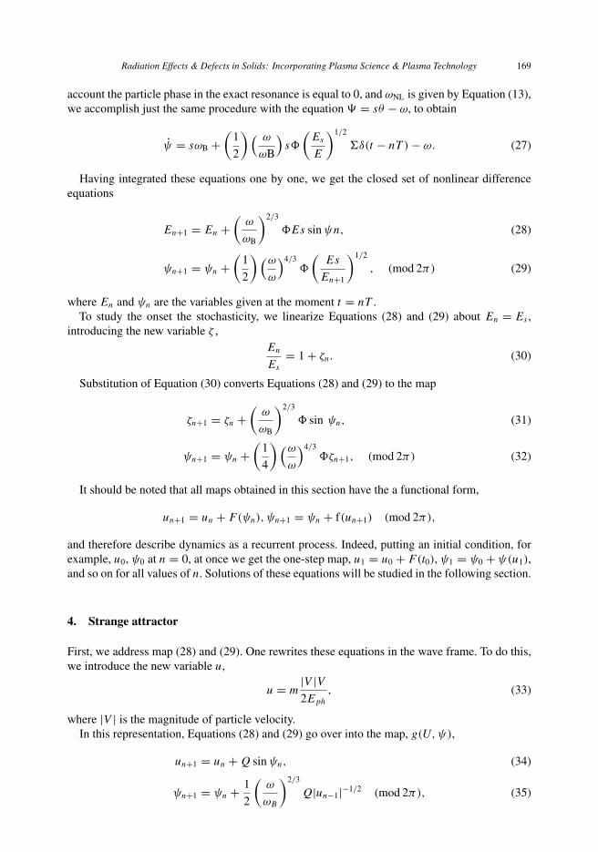
initial conditions were chosen in a random fashion and corresponded to the region of small valuesof (ψ, u). Figure 1 shows some of our results computed for one trajectory in the ψ − u phasespace. The figure shows that the boundary of {u} is well approximated by formula (43).


Figure 1. The phase space of the map. One single trajectory of length 104 for different values of Q. (a) Q = 16 and(b) Q = 32.

The existence of upper bound implies that the given manifold is a compact space, on which wecan determine the eigenvalues λ1 and λ2, the Kolmogorov entropy, K , being a kneading invariant,

K = ln λ1, (44)

and the fractal dimension of the M ,

df = 1 − ln λ1

ln λ2. (45)

By calculating, we found K = ln[(3 + √5)/2]; therefore, the rate of a loss of information

is positive. Then we compute the fractal measure df = 1, implying that the phase curve whosetopological measure is equal to one evenly fills all obtainable phase space. By virtue of theseinvariants, the pair (M, g) is an SA tightly embedded in the phase space at n → ∞.

We have found in Section 3 that transition of a given system to chaotic motion can be describedby the set of difference equations ((31) and (32)).

It is clear, that by rescaling ξ → (1/4)(ω/ωn)4/3�ξ , these equations are reduced to the map:

ξn+1 = ξn + 1

4

(ω

ωB

)2

�2 sin n, (46)

n+1 = n + ξn+1(mod ω), (47)

having the form of a standard map (7, 8). We will again use topological methods to study thebehavior of the map. First, we compute the trace of Jacobian of the map,

tr J =(

�ω

2ωB

)2

(48)

When this expression satisfies Equation (41), we find

�c = uc

Eph

= 2ωB

ω, (49)

the minimal value of the wave field required for the onset of stochastic motion.


Now substituting Equation (49) into Equation (43), we write down the simple expression forthe upper boundary of spectrum,

|ub| = E

Eph

=(

�

�c

)4/2

. (50)

Let us consider the dynamics of ions in an MH wave at the LH frequency, ωLH. In thiscase, we must set everywhere in our formulas ωB = �i, ω = ωLH = √

�i�e, where �i �e isthe gyrofrequency of an ion (electron).

Finally, Equation (49) takes the form

Uc = 2

(me

mi

)1/2

Eph, Eph = miv2ph

2, (51)

and as it appears from Equations (50) and (51), the feasible extent of particle heating is

E =(

2π

(mi

mc

)1/3)4/3

Eph. (52)

5. Heating of ions by the LH wave

Introduce the distribution function f (E, t) on the stochastic set, the evolution of which obeys theFPK equation,

∂f (E, t)

∂t= 1

2

∂

∂EDE

∂f (E, t)

∂E. (53)

Here DE is the coefficient of diffusion in energy space given by

DE = (En+1 − En)2

T, (54)

where 〈·〉 is the operator of phase average, En+1 − En is given by the original map (34) and (35)and T = 2π/�i is the ion gyroperiod.

Making use of the map in Equation (54), we get

DE = 2

(me

mi

)1/3 (�

�c

)2

E2ph/T . (55)

The function f (E, t) is positive on the SA, and beyond the SA, both the function and its derivativeare equal to zero. Therefore, the function, or rather the probability density, obeys the norm∫ Eb

Eph

f (E, t)dE = 1. (56)

Under the conditions, the steady-state solution to Equation (53) is

f (E) = 1

Eb − Eph

, (57)

and the characteristic time for establishing the distribution is found to be

td = E2b

DE=

(mi

mc

)1/3 (�

�c

)2/3

T . (58)

We have employed in Equation (58) the relations (50) and (55).


The f (E) as expected does describe a uniform distribution on the SA and determines the energyspectrum of a particle. One points out the feature of the distribution near the transition to chaos.If � → �c, then Eb → Eph and f (E) → δ(Eb − Eph), δ is the Dirac delta function, reflectingthe bifurcation transition to chaos. Like this, �c is the bifurcation parameter.

The distribution permits calculating the means

〈E〉 =∫ Eb

Eph

f (E)EdE = 1

2(Eb + Eph), (59)

〈E2〉 = 1

3(E2

b + EbEph + E2ph), (60)

and the relative level of fluctuations,√(√〈E2〉 − 〈E〉2)√〈E2〉 = 0.5, (61)

for � � �c.The distribution f (E) as well as all means through the very high level of fluctuations are strong,

stable due to the global stability of the SA.The most interesting feature of the system is the dependence of td on the magnitude of wave

field. As it follows from Equation (58), td ∝ (�(�c))2/3, while this dependence is typically a

decreasing function of �. This feature is conditioned by the properties of map itself having anexplicit dependence on the wave field in the ψ-equation. This property is irreducible due to thedegeneracy of original linear problem.

Let us discuss how the system approaches the SA. Introducing the second moment, 〈E2〉 =∫E2f (E, t)dE, we integrate Equation (53) to find with the help of Equations (55) and (56),

d〈E2〉df

= DE, (62)

that is, the particle heating is realized by a Brownian process, Eα√

t , and the heating rate isapproximately given by

dE

dt= T −1

(me

mi

)1/3

�(�c)2Eph

(Eph

E

). (63)

Note that the diffusion in energy space is accompanied by the space diffusion across an externalmagnetic field. Indeed, gyroradius r and the particle energy E are directly connected by the relation

r2 = 2E/m�2i . (64)

Utilizing Equation (63) in Equation (64), we have the cross-field coefficient

d〈r2〉dt

= D0

(Eph

E

), D0 =

(me

mi

)1/3 (Eph

m�iπ

).

6. Application

First we address the problem of particle acceleration by waves at the front of perpendicularcollisionless shock. The shock front is sufficiently steep, and the electrostatic potential is localized


at the front, the width of which is typically of the order of an inertial length. In shock surfing,the particle accelerates along the shock front under the action of the convective electric field ofthe plasma flow to v ∼ vf in a time τ ∼ vf\�i, where vf is the front speed. Then an ion withv ∼ vf ∼ ω/k can be trapped by wave field at the bottom of the potential. Remaining close to thepotential bottom, the ion is accelerated by the electric field of wave, Eω, as ever the condition

Eω > vpB (65)

is fulfilled (8).Again we have identified above the test for electric field of MH waves, which is necessary for

the acceleration to occur. Thus, using Eω = k�, Equation (49) results in (Eω)c = vpB, whichis similar to Equation (65). Furthermore, we have established that in wave fields satisfying thecondition, ion motion becomes chaotic and leads to stochastic heating of particles. In accordancewith Equations (52) and (58), particles are accelerated very rapidly as particles are heated to Eb

in about 100 gyroperiods.Note, particle simulations (11) indicate that electron acceleration by the upper-hybrid wave can

occur in this regime.At last, it should be noted that the effects related to a finite age and size of the shock and the

particle loss because scattering can modify the energy spectrum, while the heating rate as a ruleremains the same (12).

Ion heating by two electrostatic waves in the LH range was proposed by Benisti et al. (5). Theauthors demonstrated that ions with an arbitrary low initial velocity can be accelerated through anonlinear interaction with a pair of waves that obey beating criterions

ω2 − ω1 = ωB. (66)

Because of the lack of a threshold for the initial ion velocity, this acceleration scheme could bepromising to many applications, such as plasma heating in fusion devices and spacecraft plasmapropulsion.

Afterwards, a numerical exploration of this mechanism revealed that the test (66) is necessarybut not sufficient, and a second-order perturbation analysis was carried out to define the domainsof allowed and forbidden accelerations (13). They led also to a conclusion that, despite fromrestrictions, an ion with arbitrary low velocity may benefit from this mechanism.

Following the authors, we introduce these ideas by considering their model by the methodmentioned above.

First we determine the wave field of two waves as

U(x, t) = U0(cos(k1x − ω1t) + cos(k2x − ω2t))

2= U0 cos(kx − ωt) cos(κx − υt), (67)

ω = ω1 + ω2

2, k = k1 + k2

2, v = ω2 − ω1

2, κ = κ2 − κ1

2. (68)

According to (9), we set κ = 0, which corresponds to the required vg/vp � 1, where vg is thegroup velocity. Then we introduce the action–angle variables to write equation for I ,

I = U0 cos υt∑

nJn(·) sin ψ, ψ = nθ − ωt, (69)

and an appropriate equation for the variable θ .


Now, in view of Equations (67) and (69), resonance conditions satisfy the equations

ω − sθ = 0, ω = kv, ω = ω1 + ω2

2= ωLH. (70)

As before, we assume that the conditions for adiabatic approach ψ << ψω, I << ωI are met,and write down Equation (69) at first as

I = sU0 cos υtJs(s)T sin ψ∑

δ(t − nT), T = 2π

ωB, (71)

then integrating it over one time period reduces it to the difference equation,

In+1 = In + sU0Js(s)T cos υT sin ψn. (72)

Unlike Equation (28), there occurs the term cos υT due to beat oscillations, the mean value ofwhich is equal to zero in the space of parameters.

At last, under the conditions of parametric resonance (9), υT = π and the condition

ω2 − ω1 = ωB (73)

is valid. Both Equations (70) and (73) serve as the sufficient and necessary condition for efficientinteraction, and Equation (72) and an appropriate equation for the particle phase reduce to the set,which is tantamount to (28) and (29) entirely.

Proceed to the contrary case, when vg/vp << 1. For the case, we have in Equation (69) theterm cos(xvgT ) instead of cos υT . Taking the dispersion relation

ω = ωLH1 − k2

0

2k3, k � k0, (74)

k0 = ωp

c, vg = ωLHk2

0

2k3, (75)

for a given branch of waves (1), whence, it follows ω2 − ω1 = vg(k2 − k1) for ω >> ω2 − ω1.Substituting it in the beat oscillation term, cos(vgT (k2 − k1)/2), we again arrive at the conditionfor parametric resonance coinciding with Equation (73). So we found that the acceleration schemeis identical to that given above, and therefore, it is realized, if and only if condition (49) holds.Thus, it has no advantage over the traditional one.

7. Conclusion

Using the adiabatic approach, the equations of ion motion in electrostatic field of an LH wavereduce to a map. It is shown that all solutions of the map belong to an SA, and the means(observables) on the attractor are stable, irrelevant of initial conditions. The solutions have revealedthat the condition for the onset of global stochasticity is Ec = vpB, in close agreement with thenumerical value. The estimate is larger about (mi/mc)

1/6 times than that obtained by Karney (6).The upper bound of the SA can be put in correspondence with the upper boundary of energyspectrum whose value depends only on the amplitude of wave. Chaotic motion gives rise todiffusion in energy and leads to establishing the energy spectrum, and the timescales of theprocess is of the order of tens of gyroperiods. The results have been applied to a number ofproblems, including Fermi acceleration by waves at the front of shocks, and ion cyclotron heatingin the beat-wave accelerator.


References

(1) Stix, T.M. Waves in Plasmas; AIP: New York, 1992.(2) Giacalone, J. Planet. Space Sci. 2003, 51, 659–672.(3) Kuramitsu, Y.; Krasnoselskikh, V. Phys. Rev. Lett. 2005, 94, 031102-1–4.(4) Treumann, R.; Terasawa, T. Space Sci. Rev. 2001, 99, 135–150.(5) Benisti D.; Ram, A.; Bers, A. Phys. Plasmas 1998, 5, 3224–3237.(6) Karney, C.F.F. Phys. Fluids 1978, 21 (9), 1584–1612.(7) Lichtenberg, A.J.; Lieberman, M.A. Regular and Chaotic Dynamics; Springer: New York, 1992.(8) Sagdeev, R.Z.; Usikov, D.A.; Zaslavsky, G.N. Introduction to Nonlinear Physics; Harwood Acad. Publ.: New York,

1988.(9) Arnold, V.; Arez, A. Ergodic Problems of Classical Mechanics; Benjamin: New York, 1968.

(10) Chirikov, B.V. Phys. Rep. 1979, 52, 263–379.(11) McClements, K.G.; Dieckmann, M.E.; Innerman, A.; Chapman, S.C.; Dendy, R.O. Phys. Rev. Lett. 2001, 87 (25),

255002-1–4.(12) Krotov, A.; Tel’nikhin, A. Plasma Phys. Rep. 1998, 24, 767–772.(13) Spector, R.; Choueiri, E.Y. Phys. Rev. E 2004, 69, 046402-1–9.

stochastic ion heating by the lower-hybrid waves - …defectsinsolids:...

Documents