stochastic noise in atomic force microscopy€¦ · physical review e 86, 031104 (2012) stochastic...

PHYSICAL REVIEW E 86, 031104 (2012)

Stochastic noise in atomic force microscopy

Aleksander Labuda,1 Martin Lysy,2 William Paul,1 Yoichi Miyahara,1 Peter Grutter,1 Roland Bennewitz,3 and Mark Sutton1

1Department of Physics, McGill University, Montreal, Quebec, Canada H3A 2T82Department of Statistics, Harvard University, Cambridge, Massachusetts 02138-2901, USA

3INM—Leibniz Institute for New Materials, 66123 Saarbrucken, Germany(Received 2 May 2012; published 5 September 2012)

Having reached the quantum and thermodynamic limits of detection, atomic force microscopy (AFM)experiments are routinely being performed at the fundamental limit of signal to noise. A critical understandingof the statistical properties of noise leads to more accurate interpretation of data, optimization of experimentalprotocols, advancements in instrumentation, and new measurement techniques. Furthermore, accurate simulationof cantilever dynamics requires knowledge of stochastic behavior of the system, as stochastic noise may exceedthe deterministic signals of interest, and even dominate the outcome of an experiment. In this article, thepower spectral density (PSD), used to quantify stationary stochastic processes, is introduced in the context ofa thorough noise analysis of the light source used to detect cantilever deflections. The statistical propertiesof PSDs are then outlined for various stationary, nonstationary, and deterministic noise sources in the context ofAFM experiments. Following these developments, a method for integrating PSDs to provide an accurate standarddeviation of linear measurements is described. Lastly, a method for simulating stochastic Gaussian noise fromany arbitrary power spectral density is presented. The result demonstrates that mechanical vibrations of the AFMcan cause a logarithmic velocity dependence of friction and induce multiple slip events in the atomic stick-slipprocess, as well as predicts an artifactual temperature dependence of friction measured by AFM.

DOI: 10.1103/PhysRevE.86.031104 PACS number(s): 05.40.Ca, 81.40.Pq

I. INTRODUCTION

In the original implementation of the atomic force micro-scope in 1986 [1], nanoscale forces acting on a sharp tip wereinferred by sensing the “static” deflection of the cantilever towhich the tip was tethered. Soon after, “dynamic” methods[2,3] were implemented where the cantilever was oscillatednear or at its resonance frequency; this circumvented manyof the detection noise issues that occur at low frequenciesin the static case by moving the relevant noise bandwidthinto the kilohertz range. Today, both of these atomic forcemicroscopy (AFM) methods serve the nanoscience communityand have led experiments up to the boundaries imposed bythermodynamic and quantum limits [4] of physics.

At room temperature, stochastic thermal noise dominatesthe low signal-to-noise regime of nanoscale experiments. Ifthermal noise is well understood, it can even be exploitedto extract information about the tip-sample interaction [5,6].Importantly, the signal of interest in the AFM experiment itselfmight be stochastic in nature, and understanding its statisticalproperties can lead to new measurement techniques [7,8]. Infact, measuring the variance—rather than the mean—of aphysical parameter can yield higher signal-to-noise ratio innanoscale experiments where fluctuations dominate the signalof interest [9].

Inevitably, instrumental sources of noise are also present inAFM. It is therefore imperative to have a good understandingof all the sources of stochastic noise in order to properlyinterpret the results of AFM experiments in the presence ofboth signal and noise. Furthermore, understanding the sourcesof noise naturally leads to improvement of future instrumen-tal design, and serves in the optimization of experimentalprotocols.

Given the growing complexity of AFM techniques, nu-merical simulations of AFM experiments help to understand

the effects that instrumental parameters [10,11] and complexcantilever dynamics [12] have on the acquired signals. So far,virtual AFM simulators, such as VEDA [13], are optimized fordeterministic calculations of cantilever dynamics. The nextnatural step is the inclusion of stochastic cantilever dynamics,as well as stochastic vibrations inherent to the instrument andcolored detection noise, in order to more accurately reproducetrue AFM experiments.

Therefore the goal of the statistical noise analysis presentedin this paper is to provide a framework for the criticalunderstanding of variability in data acquired by AFM, toprovide AFM design guidelines for the minimization of noisein different types of experiments, to help optimize availableparameters when constructing experimental protocols, and toestablish statistical foundations for the simulation of stochasticnoise in AFM.

The next section provides an overview of stochastic noisesources in AFM. Afterwards, a case study friction experimentis presented that will be referred to throughout the discussionof the four core sections. The first section describes thedetection noise sources in AFM and how they scale with keyexperimental parameters. The second outlines the statisticalproperties of different types of noise sources in relation totheir power spectral densities (PSDs). This leads to a methodfor integrating the PSDs to obtain quantitatively accurateestimates of the variance of linear measurements, presentedin the third section. For nonlinear measurements, the fourthcore section demonstrates the utility of a method for stochasticsimulation of noise in AFM.

II. OVERVIEW OF STOCHASTIC NOISE IN AFM

In a recent article [14], the noise sources of AFM weredivided into three categories: detection noise, force noise, anddisplacement noise.

031104-11539-3755/2012/86(3)/031104(18) ©2012 American Physical Society

http://dx.doi.org/10.1103/PhysRevE.86.031104

ALEKSANDER LABUDA et al. PHYSICAL REVIEW E 86, 031104 (2012)

Optical shot noise sets the fundamental limit of detection ofthe optical beam deflection method [15], and its reduction hasplayed a primary role in enabling atomic resolution imagingwith dynamic AFM in liquids [16], for example. Detectionnoise can have a measurable impact on the tip-sample physicsand the outcome of an experiment by inducing unwantedvibrations when using feedback to track the tip-sampleseparation. Conversely to dynamic AFM, the detection noise instatic AFM is far from white and can have an elaborate spectraldistribution and be characterized by the enigmatic 1/f noise[17,18], power-line noise, various mechanical resonances, etc.Noise analysis in this situation becomes nontrivial becauseof the complicated spectral distribution of densities, whichare poorly described by parametric physical models and mustgenerally be estimated nonparametrically.

Force noise is mainly caused by thermal fluctuations whichset a fundamental lower bound to the force fluctuations that thetip imparts on a sample during a measurement. Force noise canhave a sizable impact on the outcome of an AFM experiment;for example, thermal fluctuations of the cantilever directlyaffect the maximal force observed in stick-slip measurements[19]. Thermal noise has a theoretical lower limit set bythermoelastic damping in vacuum environments [20–22]. Inambient conditions, it correlates with viscous damping [23–25]and can completely dominate detection noise in highly viscousenvironments [26]. Recently, the low-frequency fluctuationsof cantilevers have been under scrutiny: structural dampingcauses a 1/f power spectral density in the cantilever atlow frequencies where viscous forces are negligible [27];1/f noise can also be induced by the coupling of lightpower fluctuations to cantilever bending by thermally inducedstress [14].

On the other hand, the sources of displacement noise inAFM are usually not of fundamental interest because theyrelate to instrument design and AFM engineering [28]. Never-theless, their existence should not be disregarded: vibrationsbetween the tip and the sample can have profound impact onthe results of an AFM experiment, even if they lie outside of themeasurement bandwidth. For example, deliberate tip-samplevibrations can enable dynamic superlubricity [29,30] andeliminate wear [31] in friction experiments. By the sametoken, undesirable vibrations of the tip-sample junction canaffect the results of an AFM experiment well beyond simpledeterioration of image quality.

III. CASE STUDY

This section presents a static AFM experiment which willserve as an example to guide the noise analysis of the followingsections. A friction measurement was chosen as the benchmarkbecause it represents a simple example of a linear measurementin static AFM.

Friction force microscopy [32] in liquid environmentshas recently reached atomic-scale resolution [33,34] withclear measurements of stick-slip tip motion acquired duringthe electrochemically activated transition between a copperchloride monolayer and Au(111), as shown in the image ofFig. 1. The lateral force curves in Fig. 1(a) demonstrate thatroughly 2 eV of energy is elastically stored and released forevery stick-slip cycle. However, roughly 50 meV is dissipated

FIG. 1. (Color online) (a) A backward and forward lateral forcescan is performed on Au(111), with a scan rate of 25 lines/s whichcorresponds to ∼400 nm/s. The tip scans over the surface with stick-slip motion. Average lateral forces are shown in dotted lines. Thearea enclosed in the hysteresis loop is the energy lost due to friction.(b) A lateral force map is shown (right) with the calculated frictionforce per line (left) as a function of time; the copper chloride layeris electrochemically desorbed at t = 0 s, resulting in a change inobserved lattice and a reduction in both friction average and standarddeviation. (The slight kink at t = 5 s is caused by the change in imagescan direction from downwards to upwards—two consecutive imageswere merged for this figure.)

during every stick-slip cycle, as determined by measuringthe area enclosed by the hysteresis loop. The correspondingaverage friction force per line is plotted in Fig. 1(b), anddemonstrates a clear reduction in friction on Au(111) vs thecopper monolayer [33]. In the following sections, attention isfocused on the variability in friction which gives rise to thefollowing questions:

(i) Does the variability originate due to detection noise, oris it a true measurable variability in friction?

(ii) What are the origins of detection noise, and can it bereduced?

031104-2

STOCHASTIC NOISE IN ATOMIC FORCE MICROSCOPY PHYSICAL REVIEW E 86, 031104 (2012)

(iii) Is the true friction variability enhanced by vibrationsof the instrument?

IV. NOISE IN OPTICAL BEAM DEFLECTION:THE POWER SPECTRAL DENSITY

This section introduces the “power spectral density” (PSD)in the context of analyzing noise of the optical beam deflection(OBD) method [15]. The PSD, sometimes referred to as thepower spectrum, represents a frequency decomposition of thepower of a signal. It is particularly suitable for quantifyingstationary stochastic processes. The PSD will be central to theremainder of the document, and will first be presented in thissection from an experimental point of view.

The OBD method is the most widely used detection methodin AFM. Our AFM [33,35] employs a 1-mW fiber-coupled su-perluminescent diode (SLD). Like any light source, SLDs areafflicted by both angular fluctuations and power fluctuationsof their emitted light beam. Understanding how both angularfluctuations and power fluctuations affect AFM measurementspermits the optimization of experiments by the reduction ofdetection limits, and enables accurate interpretation of noiseobserved in AFM experiments.

In the most common application of the OBD method, the re-flected light beam shines onto a split-diode photodetector. Thedifference in power between both sides of the photodetectoris proportional to the angular deflection of the cantilever—tofirst order. As long as the light beam is perfectly centered onthe photodetector, the detection of its position is practicallyimpervious to power fluctuations. The differential nature ofthe measurement results in a high common-mode rejectionratio: the difference signal remains at zero even if the totaloptical power fluctuates.

Whereas this is a good approximation for dynamic AFM,static AFM is often performed under varying loads that causea large nonzero difference signal during the experiment.Consequently, the detection power spectral density n2

�(f )can vary throughout a static AFM experiment because it isa function of the time-averaged normalized difference signal�0. The noise is minimized when �0 = 0, and increases as|�0| > 0. The generalized form n�(f |�0) is measurable andpredictable, as is demonstrated in the following section. Notethat dynamic AFM can also be prone to the same problems ifthe light beam is not perfectly centered on the photodetector.

A. Common-mode and differential-mode noise

Consider some irradiance profile I (θ ′) of a light beamshining on a split photodetector, where θ ′ is the angularcoordinate in the far field. The integrated power incidenton each section of the photodetector, PA and PB , is used togenerate the normalized difference signal

�(t) = PB(t) − PA(t)

P0, (1)

which provides a measure of cantilever deflection, and thenormalized sum signal

�(t) = PA(t) + PB(t)

P0, (2)

− 00020.

− 00010.

0

0.0001

0.0002

norm

aliz

ed d

iffe

renc

eΔ

0 0.2 0.4 0.6 0.8 1

0.998

0.999

1

1.001

1.002

time (s)

norm

aliz

ed s

umΣ

FIG. 2. (Color online) The normalized difference (�) and nor-malized sum (�) of our SLD light beam centered on the photodetector.Note that both vertical axes differ by a factor of 10 × in range. The� fluctuations are roughly 10 × larger and strongly afflicted by linenoise (60 Hz and harmonics). Both signals are uncorrelated. Thedetails of the optical beam deflection system and electronics used forthis measurement are outlined elsewhere [33,35].

where P0 is the total optical power time averaged across theentire experiment.

Figure 2 shows data acquired during 1 s of both signals in thesituation where the light beam is centered on the photodetector:�0 = 0, where �0, defined earlier, is the time-averagedvalue of �(t). In this situation, any instantaneous fluctuationδI (θ ′) of the irradiance profile can always be mathematicallydecomposed into two orthogonal components:

δI (θ ′) = δICM + δIDM. (3)

The common-mode irradiance fluctuation δICM refers tothe symmetric component of δI for which the deviations fromthe time-averaged irradiance I0(θ ′) cause changes in the sumsignal δ�, but no change in the difference signal δ� = 0.Likewise, the differential-mode irradiance fluctuation δIDM isantisymmetric, causes no net change in total optical power(δ� = 0), and results only in a deviation δ� which appearsas a change in the measured angle. Figure 3 illustrates thisdecomposition.

Certain noise sources may cause deviations of only δIDM

or δICM or both. For example, shot noise causes the sameamount of power fluctuation in both δIDM and δICM because itis spatially uncorrelated on all length scales. On the other hand,angular movement in the light beam causes only δIDM with noassociated changes in total power because the fluctuation isperfectly spatially correlated (loss of light on one detectorimplies gain of light on the other detector). In the special caseof �0 = 0 discussed so far, both of these fluctuations in theirradiance profile can be considered orthogonal, and thereforeall fluctuations in δ� and δ� are effectively temporallyuncorrelated—assuming that δ� � 1 and δ� � 1 such thatcross-terms δ�δ� ≈ 0. Note that both time series in Fig. 2show no (temporal) correlation.

031104-3


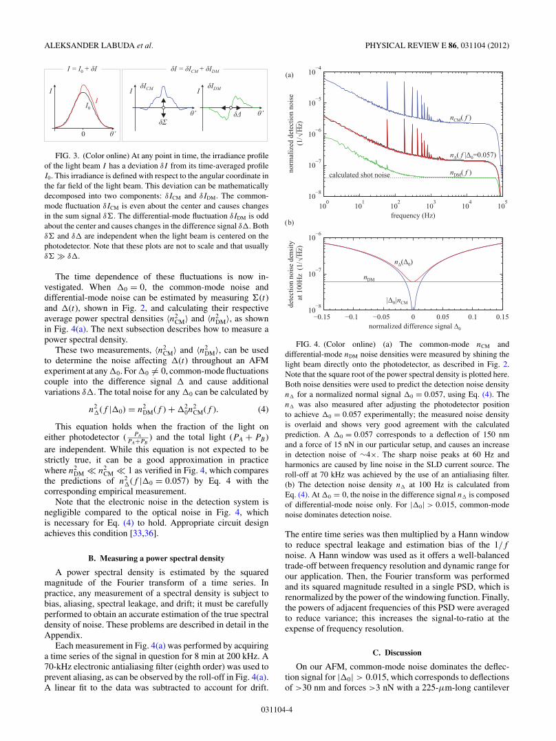
FIG. 3. (Color online) At any point in time, the irradiance profileof the light beam I has a deviation δI from its time-averaged profileI0. This irradiance is defined with respect to the angular coordinate inthe far field of the light beam. This deviation can be mathematicallydecomposed into two components: δICM and δIDM. The common-mode fluctuation δICM is even about the center and causes changesin the sum signal δ�. The differential-mode fluctuation δIDM is oddabout the center and causes changes in the difference signal δ�. Bothδ� and δ� are independent when the light beam is centered on thephotodetector. Note that these plots are not to scale and that usuallyδ� � δ�.

The time dependence of these fluctuations is now in-vestigated. When �0 = 0, the common-mode noise anddifferential-mode noise can be estimated by measuring �(t)and �(t), shown in Fig. 2, and calculating their respectiveaverage power spectral densities 〈n2

CM〉 and 〈n2DM〉, as shown

in Fig. 4(a). The next subsection describes how to measure apower spectral density.

These two measurements, 〈n2CM〉 and 〈n2

DM〉, can be usedto determine the noise affecting �(t) throughout an AFMexperiment at any �0. For �0 = 0, common-mode fluctuationscouple into the difference signal � and cause additionalvariations δ�. The total noise for any �0 can be calculated by

n2�(f |�0) = n2

DM(f ) + �20n

2CM(f ). (4)

This equation holds when the fraction of the light oneither photodetector ( PA

PA+PB) and the total light (PA + PB)

are independent. While this equation is not expected to bestrictly true, it can be a good approximation in practicewhere n2

DM � n2CM � 1 as verified in Fig. 4, which compares

the predictions of n2�(f |�0 = 0.057) by Eq. 4 with the

corresponding empirical measurement.Note that the electronic noise in the detection system is

negligible compared to the optical noise in Fig. 4, whichis necessary for Eq. (4) to hold. Appropriate circuit designachieves this condition [33,36].

B. Measuring a power spectral density

A power spectral density is estimated by the squaredmagnitude of the Fourier transform of a time series. Inpractice, any measurement of a spectral density is subject tobias, aliasing, spectral leakage, and drift; it must be carefullyperformed to obtain an accurate estimation of the true spectraldensity of noise. These problems are described in detail in theAppendix.

Each measurement in Fig. 4(a) was performed by acquiringa time series of the signal in question for 8 min at 200 kHz. A70-kHz electronic antialiasing filter (eighth order) was used toprevent aliasing, as can be observed by the roll-off in Fig. 4(a).A linear fit to the data was subtracted to account for drift.

FIG. 4. (Color online) (a) The common-mode nCM anddifferential-mode nDM noise densities were measured by shining thelight beam directly onto the photodetector, as described in Fig. 2.Note that the square root of the power spectral density is plotted here.Both noise densities were used to predict the detection noise densityn� for a normalized normal signal �0 = 0.057, using Eq. (4). Then� was also measured after adjusting the photodetector positionto achieve �0 = 0.057 experimentally; the measured noise densityis overlaid and shows very good agreement with the calculatedprediction. A �0 = 0.057 corresponds to a deflection of 150 nmand a force of 15 nN in our particular setup, and causes an increasein detection noise of ∼4×. The sharp noise peaks at 60 Hz andharmonics are caused by line noise in the SLD current source. Theroll-off at 70 kHz was achieved by the use of an antialiasing filter.(b) The detection noise density n� at 100 Hz is calculated fromEq. (4). At �0 = 0, the noise in the difference signal n� is composedof differential-mode noise only. For |�0| > 0.015, common-modenoise dominates detection noise.

The entire time series was then multiplied by a Hann windowto reduce spectral leakage and estimation bias of the 1/f

noise. A Hann window was used as it offers a well-balancedtrade-off between frequency resolution and dynamic range forour application. Then, the Fourier transform was performedand its squared magnitude resulted in a single PSD, which isrenormalized by the power of the windowing function. Finally,the powers of adjacent frequencies of this PSD were averagedto reduce variance; this increases the signal-to-ratio at theexpense of frequency resolution.

C. Discussion

On our AFM, common-mode noise dominates the deflec-tion signal for |�0| > 0.015, which corresponds to deflectionsof >30 nm and forces >3 nN with a 225-μm-long cantilever

031104-4


having a 0.1 N/m spring constant. This stresses the importanceof centering the light beam on the photodetector before theexperiment, such that �0 = 0 corresponds to 0 nN. Typically,experiments that are performed near 0 nN are most prone todetection noise and can benefit from the high common-moderejection ratio at �0 = 0. Centering the light beam in thelateral direction is equally important for sensitive frictionexperiments.

The common-mode noise is fundamentally limited bysource-induced noise, which exceeds shot noise by nearly tentimes for our particular SLD, as calculated theoretically byRef. [37]. In practice, the measured common-mode noise inFig. 4 is actually dominated by electronic noise in the currentdriver which rolls off above 70 kHz, and has the characteristic60-Hz harmonic noise peaks and the elusive 1/f noise at lowfrequencies. In either case, for drive-current or source-inducednoise, experiments performed at |�0| > 0.015 do not benefitfrom an increase in optical power because they are not limitedby optical shot noise.

Figure 4(b) demonstrates that differential-mode noise dom-inates the detection noise for |�0| < 0.015, and that shotnoise only takes effect for frequencies above a few hundredhertz. Consequently, changing the optical power by eitherboosting the drive current or coating the cantilever reducesonly shot noise, such that only fast experiments performed at|�0| < 0.015 benefit from an increase in optical power (anexact quantification of “fast” is the topic of Sec. VI). At lowfrequencies, the angular fluctuations of the light beam aremeasurable above shot noise. These fluctuations are spatiallyuncorrelated and intrinsic to the light beam as it exits the opticalfiber; therefore they are independent of the AFM design anddepend only on the specific light source.

These observations suggest that discussing the fundamentaltheoretical limits of OBD noise in static AFM experimentsis not necessarily worthwhile, because they might be over-shadowed by other noise sources in experimental settings.The differential-mode noise may be limited by 1/f noise,rather than shot noise, and the drive electronics may set thecommon-mode noise limit far above the shot noise or evensource-induced noise. It is therefore advisable to empiricallymeasure the common-mode and differential-mode noise forany particular setup and use the modeling summarized byEq. (4) to make well-informed predictions about detectionnoise in AFM experiments.

So far, noise has been quantified by its power spectraldensity. At this stage, it is unclear how all the componentsof the PSD in Fig. 4 relate to the variability in the measuredfriction seen in Fig. 1. White noise, 1/f noise, and line noiseall have unique statistical properties and dominate at differentfrequencies. The statistical interpretation of a PSD is the topicof the following section.

V. STATISTICS OF THE POWER SPECTRAL DENSITY

This section outlines the statistical properties of differentnoise sources in AFM, with the goal of performing meaningfulnoise analysis of linear measurements (Sec. VI) and efficientstochastic noise simulations (Sec. VII), using the powerspectral density (PSD).

The statistical analysis in this section relates to stationarynoise, defined as a stochastic process with an underlying prob-ability distribution that does not vary in time. The covariancebetween any two outcomes of such a process depends onlyon the relative time separating their measurement, and isindependent of absolute time. The mean must remain constant.

In contrast, nonstationary noise, such as vibrations causedby sporadic slamming of a door or intermittent discussionsin the laboratory, does not constitute a fundamental detectionlimit in AFM and will be disregarded. Also, 1/f noise isnonstationary, but it can be approximated as stationary givencertain conditions that will be discussed later. Linear driftis neither stochastic nor stationary on any time scale, andtherefore cannot be described by a PSD; it should always besubtracted from the time signal before calculating a PSD (seeAppendix for details).

Most fundamental noise sources in AFM can be approxi-mated as stationary with high accuracy, which will be assumedhenceforth.

A. Noise in the time domain

Let xt = [x1,x2, . . . ,xm]′ be a m × 1 vector of randomvariables, acquired on an equally spaced time-domain basist = [t1,t2 . . . tm]. This is the form in which data are acquiredby an analog-to-digital converter (ADC) card used in mostmodern data acquisition systems. The data vector xt is alwayscorrupted by stochastic noise, and can therefore be expressedas the sum of deterministic (dt ) and random (ε t ) components:

xt = dt + ε t , (5)

where the “t” subscript emphasizes that these vectors aredefined in the time domain. Note that vectors in bold representvectors of random variables which have some associated prob-ability density function, while dt represents a nonprobabilisticdata vector. Further in this section, ε t will be used to representa single measurement drawn from the probability distributionof ε t .

The distinction between dt and ε t is a matter of perspective:for example, stochastic thermal fluctuations of the cantilevercan be considered noise (ε t ) or signal (dt ) in differentsituations. If an experiment seeks to determine a hydrationlayer structure by its effect on the thermal motion of thecantilever [5], this thermal motion can be considered adesirable experiment signal corrupted by some stochasticdetection noise. On the other hand, the measurement of forcesexerted by a single titin molecule tethered to the cantilevertip [38] is clearly corrupted by undesirable stochastic thermalnoise of that cantilever.

Assuming the noise ε t has zero mean, the measurementof interest dt is equal to the expectation value of xt , whichhas some unwanted variability characterized by a temporalcovariance matrix Vt :

Vt = Var(xt ) = E(ε t · ε†t ) = σ 2

⎡⎢⎢⎢⎢⎣

1 ρ2 ρ3 . . .

ρ2 1 ρ2 . . .

ρ3 ρ2. . . . . .

......

... 1

⎤⎥⎥⎥⎥⎦ , (6)

031104-5

ALEKSANDER LABUDA et al. PHYSICAL REVIEW E 86, 031104 (2012)edutilp

ma

time

ytisned rewop

frequency

(a) noise in the time domain

(b) noise in the frequency domain

t

⟨ ⟩|n| 2

2

f t t= ( · )† † ⟨ ⟩Vf

t t t= · † ⟨ ⟩Vt

color legend (logarithmic) 1−1 0.01−0.1 0.1−0.01

|n|

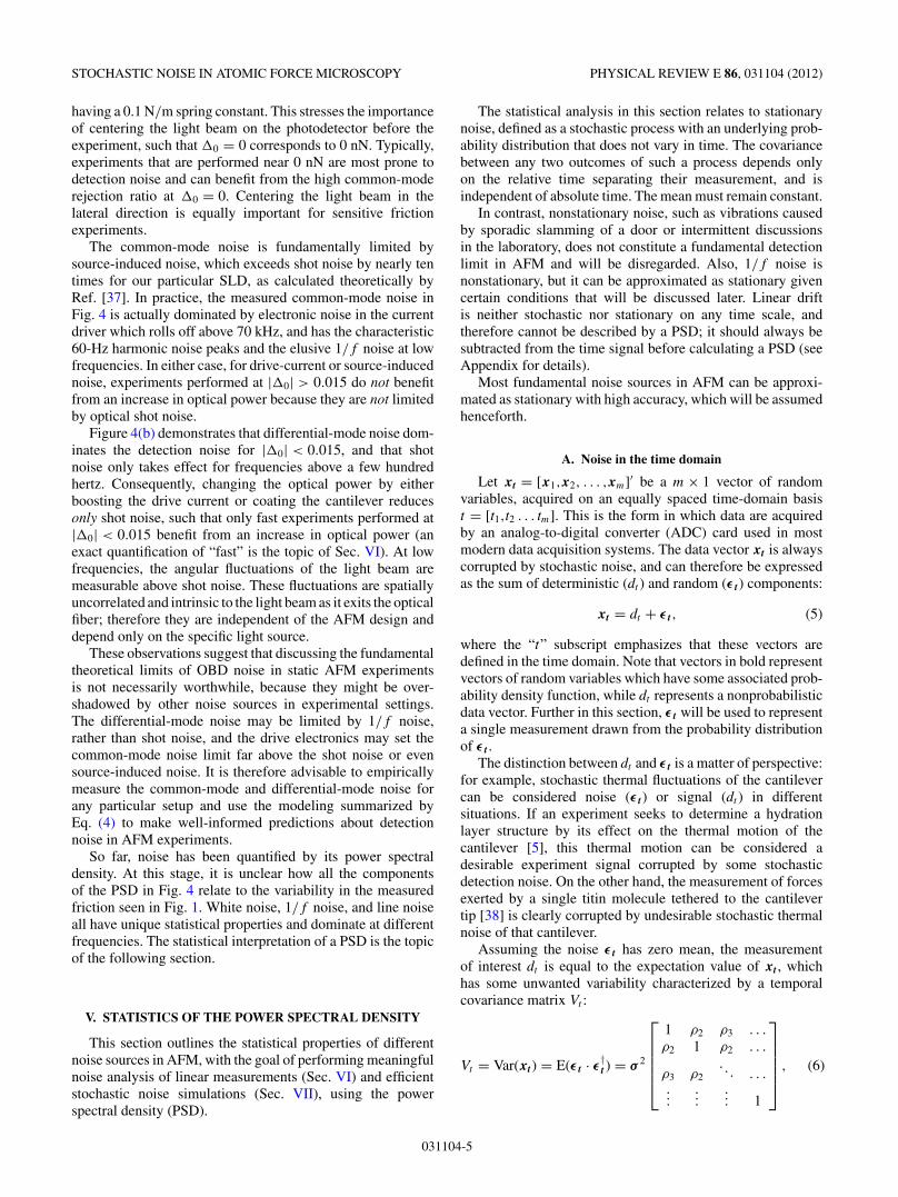
FIG. 5. (Color online) A thermally driven harmonic oscillatorwith Q = 10 is used as an example to illustrate the key differencesbetween performing noise analysis in the time and frequencydomains. (a) A single time series is shown, with a correspondingtemporal power matrix Vt , many of which can be averaged 〈Vt 〉 toestimate the temporal covariance matrix Vt . The latter has significantoff-diagonal elements due to correlations between data points in thetime domain. (b) A single power spectral density n2 and the average〈n2〉 of 1000 is shown, with the corresponding spectral power matrixVf and its average 〈Vf 〉 which is asymptotically diagonal becausethe noise is stationary. For simplicity, only the real part of the firstquadrant of the matrices is shown. 〈Vt 〉 and 〈Vf 〉 were averaged 1000times.

where “†” represents the conjugate transpose, while Var and Eare the variance and expectation value operators. Note that Vt

is a Toeplitz matrix (identical elements across each diagonal)which is required for the time invariance property of stationarynoise.

The matrix Vt is a theoretical quantity which can only beestimated experimentally. A single outcome εt drawn fromthe probability distribution of ε t results in a temporal powermatrix defined as Vt = εt · ε

†t . The average 〈Vt 〉 asymptotically

converges to the temporal covariance matrix Vt . This isillustrated in Fig. 5(a) for a thermally driven harmonicoscillator.

In the special case of white noise, statistics are straight-forward: all the off-diagonal elements of Vt are zero becauseevery data point in ε t is uncorrelated. For nonwhite noise, thetime-domain random variables are correlated, with associatedoff-diagonal covariance elements in Vt , as seen in Fig. 5(a).This makes the time domain a poor basis for performing noiseanalysis.

For example, a single friction measurement in Fig. 1 isa linear combination of the 1024 data points recorded in alateral force loop: average forward lateral force minus averagebackward lateral force. In the case of white noise, the standarddeviation of friction is simply the standard deviation of lateralforce divided by

√1024. However, in the presence of pure

1/f 2 noise, for example, this approach is wrong and wouldunderestimate the standard deviation of friction by nearly 8×.This error stems from the strong correlation of noise in thetime domain; in short, covariances cannot be neglected if thenoise is not white.

In the next section, variances will be decorrelated bytransferring the noise analysis into the frequency domain.

B. Noise in the frequency domain

The signal xt in the time domain can be mapped into thefrequency domain by the linear transformation known as thediscrete Fourier transform:

x f = Fxt , (7)

where F is the complex-valued Fourier matrix. If the units ofxt are V , then the units of x f are V/

√Hz. The decomposition

of the frequency-domain measurement x f into signal and noisecomponents remains valid due to linearity, and follows fromEq. (5) as

x f = Fdt + Fε t = df + ε f . (8)

Although it might be more difficult to interpret thefrequency-domain signal df , the interpretation of stationarynoise ε f becomes much simpler because the correspondingspectral covariance matrix Vf is (asymptotically1) diagonaliz-able:

Vf = Var(x f ) = E(ε f · ε†f ) =

⎡⎢⎣

σ 21 0 0

0. . . 0

0 0 σ 2m

⎤⎥⎦ . (9)

In essence, the frequency domain represents the orthogonalbasis of stationary noise [39], which accurately representsmost noise sources in AFM. Because the random variablescomposing x f are uncorrelated, their variances can be addedwithout consideration of any off-diagonal terms. This makesthe frequency domain an attractive basis for noise varianceanalysis. In analogy to the time domain, the spectral covariancematrix Vf is experimentally estimated by averaging thespectral power matrix Vf = ε f · ε

†f . This is illustrated in

Fig. 5(b), where 〈Vf 〉 is shown to converge to the diagonal Vf .The power spectral density is the diagonal of the spectral

covariance matrix Vf , which provides a complete statisticaldescription of any stationary Gaussian noise. If the noise is sta-tionary but non-Gaussian, further assumptions are necessaryfor a full characterization. However, meaningful noise varianceanalysis can still be performed on non-Gaussian stationarynoise using the power spectral density, as will be shown in thenext subsection.

1The term “asymptotically diagonalizable” refers to the fact thatthere is a true diagonal Vf defined in continuous time that can beapproximated in discrete time to arbitrary accuracy as m → ∞. Inexperimental AFM settings, where m is usually in the hundreds oreven millions, this approximation is often overshadowed by the finiteprecision in estimating discrete time Vf .

031104-6


FIG. 6. (Color online) Four different stationary noise sources are analyzed. A single outcome is drawn, and histogrammed. Noise can havea Gaussian (a),(b) or a non-Gaussian (c),(d) probability density function, as overlaid on the histogram. Although flicker noise is non-Gaussian,it is stationary and therefore has a 〈Vf 〉 which is asymptotically diagonalizable and a well-defined power spectral density. The rectified linenoise is non-Gaussian and is only stochastic because it has a random phase. All harmonics are locked in phase, but since the noise is stationary,the analysis of variance using the power spectral density still holds.

Figures 6(a) and 6(b) shows examples of two stationaryGaussian noises: white noise and a thermally driven dampedharmonic oscillator. The Gaussian property is illustratedby the histograms, which show convergence to a normaldistribution in the time domain. Even though the harmonicoscillator has highly correlated data in the time domain, bothspectral covariance matrices are diagonal, and therefore thepower spectral densities describe these Gaussian noise sourcescompletely.

Figure 6(c) depicts flicker noise [40], defined here as atwo-state process with a switching time that is exponentiallydistributed. Although purely stochastic and stationary, thisbimodal process is far from Gaussian, yet the spectralcovariance matrix is diagonal because the process is stationary,and therefore an accurate analysis of variance can be performedin the frequency domain.

Figure 6(d) represents rectified line noise, modeled as theabsolute value of a sine wave. Although stationary, its onlystochastic component is the random phase. Such a noise sourceis very spectrally pure, and defined only by the fundamentalfrequency and harmonics. Despite the fact that the PSD hasonly deterministic harmonic powers, the spectral covariancematrix is still diagonal and the analysis of variance presentedin the following section holds. Note that spectral leakage hasbeen disregarded in the discussion so far because it can bemade arbitrarily small by appropriate averaging methods (seeAppendix).

C. Probability distribution of the power spectral density

This description begins with the special case of stationaryGaussian noise, and is later extended to stationary non-Gaussian noise. The limitations in statistically characterizing1/f noise, which is nonstationary, are also discussed. Finally,the behavior of deterministic noise under stationary noiseanalysis is investigated.

1. Stationary Gaussian noise

Each random variable composing the frequency-domainnoise vector ε f is a linear combination of all the randomvariables in the time-domain noise vector ε t , as weighted bythe complex-valued Fourier matrix F . Since ε t is normallydistributed for Gaussian noise, the real and imaginary randomvariables of ε f are also normally distributed, and any twofrequencies are asymptotically independent for m → ∞.

The power spectral density is the squared magnitude of ε f ,

n2 = diag(ε f · ε†f ) (10)

(for notational simplicity, the squaring in n2 implies squaringthe magnitude |n|2). Note that n2 is a m × 1 vector ofrandom variables with an associated probability distribution.According to Eq. (10), every component of n2 is the sumof squares of the identically distributed real and imaginaryparts of the corresponding component of ε f . From basicprobability theory, it is known that the sum of squares oftwo independent and identically distributed normal randomvariables is exponentially distributed. In other words, thepower spectral density n2 of stationary noise is composedof independent exponentially distributed random variables.

Experimentally, the expectation value E(n2) is estimatedby the average power spectral density 〈n2〉, taken over manysingle observations n2. Because of the large variance of theexponential distribution, it is important to perform manyaverages when measuring power spectral densities [41]. Notethat the averaging should be performed in power 〈|n|2〉, ratherthan in magnitude 〈|n|〉2, otherwise the PSD is underestimatedby a factor of 4/π (see Appendix for details).

2. Stationary non-Gaussian noise

Stationary non-Gaussian noise sources may also complywith the statistical properties described so far—under certainconditions. Take flicker noise, as illustrated in Fig. 2(c); eventhough the time-domain probability density function is far

031104-7


from Gaussian, the frequency-domain random variables areasymptotically normally distributed by virtue of the centrallimit theorem, and thus n2 is composed of exponentiallydistributed random variables. On the other hand, the rectifiedsine wave in Fig. 6(d) has only one random component—itsphase—and therefore does not obey the criterion for the centrallimit theorem to take effect. In fact, any two n2 for this noiseare identical; in other words, n2 is purely deterministic withno associated probability distribution (disregarding spectralleakage).

Although the power spectral density does not fully describethe statistical properties of stationary non-Gaussian noise, itis sufficient for the noise analysis of linear measurementspresented in the next section.

3. 1/f noise

Measuring 1/f noise is a nontrivial task. For exponents0 < c < 1, noise with power spectra ∼1/f c are stationary butwith long-range memory. For c � 1, the noise is nonstationary,having variance which changes with time [42]. In certain cases,the 1/f power spectrum of the noise can be approximated ona limited bandwidth, as long as its PSD is measured across amuch wider bandwidth. For nonstationary noise, however, thewindowing function must be chosen according to c in order toobtain consistent estimates.

Meanwhile, any distributional assumption such as Gaus-sianity of 1/f noise should always be verified. A commondeterministic signal leading to a 1/f noise spectrum is lineardrift. Stochastic 1/f noise and deterministic linear drift arefundamentally different sources of noise. Using the PSD torepresent linear drift is inconvenient. Estimation details in thepresence of both stochastic 1/f noise and deterministic driftare discussed in the Appendix, where it is concluded that it isbest to subtract linear drift from any signal before calculatingits PSD to more accurately estimate the 1/f noise.

4. Deterministic periodic noise

In typical AFM experiments, the relative phase of thedeterministic periodic noise is random, such that its effecton a measurement is not purely deterministic.

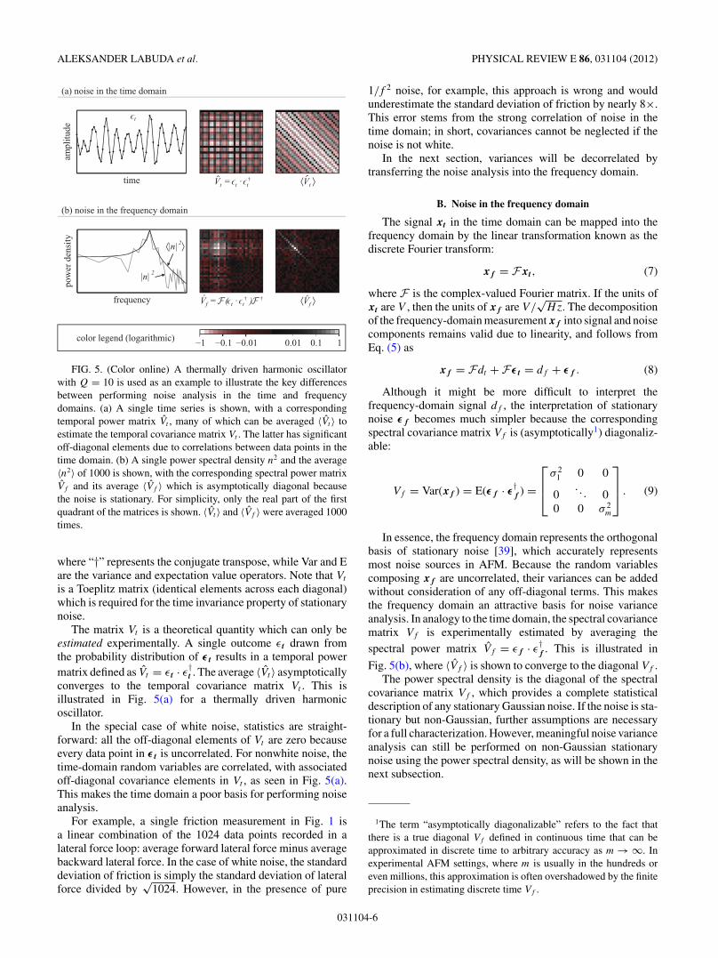
Take a square wave noise with constant amplitude and arandom phase; the power spectral density n2 of this noisesource has fixed harmonics with predetermined magnitudes(disregarding spectral leakage). Therefore, n2 is a vector ofdeterministic numbers, rather than random variables. Thefollowing simulation describes the effect of such deterministicnoise on the probability distribution of linear measurements.For illustrative purposes, a friction experiment was simulatedwith three noise sources:

(1) Deterministic noise: a deterministic square wave with aperiod equal to the scan rate. The only random component isthe relative phase of the square wave.

(2) Dephased noise: the noise from (1) was recycled buteach frequency component was given a random phase (drawnfrom a uniform distribution).

(3) Stochastic Gaussian noise: noise was generated fromthe PSD from (1), whereby each complex-valued frequencyamplitude was drawn from a complex normal distribution.This method is described in detail in Sec. VII.

deterministic noise

dephased noise

stochastic noise σ= 0.0 pN14.46 3

σ= 0.0 pN14.45 2

σ= 0.0 pN14.44 2

−40 −30 −20 −10 0 10 20 30 400

500

1000

1500

2000

2500

3000

friction error (pN)

coun

t

FIG. 7. (Color online) A friction experiment was simulated for asquare wave noise, assuming (1) a single random phase (deterministicnoise), (2) dephasing all the frequency components but keeping fixedmagnitudes (dephased noise), and (3) drawing the complex-valuedamplitudes from a normal distribution (stochastic noise). Note thatall noise sources lead to an identical standard deviation in friction,even though their probability distributions are completely different.The square wave was given an amplitude of 50 pN, and its periodwas equal to the scan rate. Note that such a source of noise would beimperceptible in the lateral force channel in Fig. 1(a) due to its smallamplitude, but could cause significant error in estimating the frictioncomputed in Fig. 1(b).

The result is presented in Fig. 7. Because the simulationwas performed with zero friction, any observed frictionis an error caused by noise. Although each noise sourceresults in completely different distributions in the observedfriction error; their standard deviations are identical. Thisdemonstrates that the analysis of variance using PSDs is oftenaccurate for any type of stationary noise source (deterministicor stochastic); however, it cannot predict the probabilitydistribution of a linear measurement unless the noise is purelystochastic and stationary, which are the assumptions requiredfor the central limit theorem in Sec. V C 2 to hold.

D. Discussion

The frequency domain is best suited for noise analysisbecause its covariance matrix is diagonal. In other words,the frequency-domain data points are uncorrelated, whiletime-domain data points are correlated if the noise is not white.This significantly simplifies the analysis of variance presentedin the next section, where variances can be added withoutconsideration of covariances.

The diagonal of the covariance matrix, defined as thepower spectral density (PSD), contains all the statisticalinformation of stationary Gaussian noise, which describesfundamental noise sources in AFM such as optical shot noiseand thermal noise. For stationary non-Gaussian noise, thePSD still provides an accurate measure of variance, but lacksinformation regarding the specific probability distribution of

031104-8


a measurement performed in the presence of such noise. Thisstatement applies to both stochastic noise, such as flicker noise,and deterministic noise, such as line noise.

The assumptions in describing thermal noise and opticalshot noise as stationary are that the temperature is fixed,and that the average optical power is fixed, respectively. Itis well known that there are fluctuations in both quantities,which set a lower limit to accuracy in describing these noisesources by their power spectral density. For example, 1/f

noise in optical power causes the shot noise level to fluctuateduring an experiment. More importantly, we are aware thatthe PSD of detection noise may vary during an experiment ifthe cantilever deflection changes (see Fig. 4). This can alsoviolate the assumption of stationarity.

For stationary stochastic noise, the data points of a PSD areindependent and exponentially distributed. The exponentialdistribution of PSD data points follows from the fact that thereal and imaginary amplitude components at a given frequencyare (asymptotically) independent and identically distributedGaussian random variables.

VI. STANDARD DEVIATION OFLINEAR MEASUREMENTS

This section outlines a method for integrating the powerspectral density that provides a quantitatively accurate stan-dard deviation of any arbitrary linear measurement.

For an accurate noise analysis, it is best to characterize thenoise of the system across a bandwidth much wider than thebandwidth used during the experiment. Ideally, the noise ismeasured from a frequency well below the scan rate (by afew orders of magnitude) and up to a frequency that exceedsthe roll-off frequency of the detection system. Accurate PSDestimation is covered in the Appendix.

A. Linear measurements in the time domain

As described in the previous section, experimental dataare typically acquired in the time domain, and recorded as am × 1 vector composed of a deterministic component (dt ) andstochastic component (ε t ), as in

xt = dt + ε t . (11)

The deterministic component contains the information ofinterest to the experimenter. A single-valued linear measure-ment ϕ is defined as any linear combination of the m valuesof xt , summarized by the dot product

ϕ = wϕ · xt , (12)

where the 1 × m vector wϕ is the measurement samplingfunction which weighs the linear combination of xt elements.Note that ϕ is a random variable as it is the weighted sum ofmany random variables.

For example, if xt is a time series of the lateral force fora single scan loop during a friction experiment (see Fig. 1),the following measurement sampling function results in theaverage friction force:

wϕ = 1

m[1,1, . . . −1,−1], (13)

FIG. 8. (Color online) (a) The measurement sampling functionfor a friction measurement wϕ , and (b) the magnitude of its Fouriertransform |kϕ |. Zero-padding of wϕ was used to increase the frequencyresolution of |kϕ |, as explained in the Appendix. (c) The powerspectral density of detection noise 〈n2〉, and the noise transfer function|kϕ |2 (overlaid in light gray for a scan rate of 10 Hz), which aremultiplied and integrated to obtain the standard deviation of a frictionmeasurement σϕ , at various scan rates as shown in (d). Detectionnoise in this friction experiment is minimized at a scan rate of ∼30Hz, where 60 Hz and harmonics are filtered out by the zeros of|kϕ |, as seen in (c). An ideal Nyquist filter at fs/2 was assumed inthis computation. In (a) and (b), only 32 data points were used todefine wϕ (prior to zero-padding) for visual clarity. In (c) and (d), a512-data-point wϕ was used to match our experiment.

with an equal number of positive and negative values as shownin Fig. 8(a). In fact, this is the measurement sampling functionfor estimating the hysteresis in a variety of AFM experiments,including force-distance spectroscopy, for example.

It is inevitable that this measurement has some variabilitycaused by true physical variability between repeated measure-ments dt and/or due to noise ε t . The topic of this sectionis to separate these two sources of variability by accuratelyquantifying the variability caused by ε t .

For linear measurements, the deterministic and stochasticcomponents are separable, which follows by combiningEqs. (11) and (12) into

ϕ = wϕ · dt + wϕ · ε t . (14)

The expectation value of the measurement is E(ϕ) = wϕ ·dt . The variance of the measurement σ 2

ϕ caused by stochasticnoise ε t is a linear combination of the elements of the m × m

temporal covariance matrix Vt .

σ 2ϕ = Var(wϕε t ) = wϕVtw

′ϕ. (15)

The following section uses the properties of stationary noiseto simplify this matrix calculation by transferring this noiseanalysis into the frequency domain.

031104-9


B. Linear measurements in the frequency domain

The variance analysis of the measurement ϕ can betransferred into the frequency domain by simply adding theidentity F−1F = I to the previous equation:

σ 2ϕ = Var(wϕF−1Fε t ) = kϕVf k†ϕ, (16)

where the noise transfer function kϕ = wϕF−1 and the spectralcovariance matrix Vf = Var(Fε t ) as defined in the previoussection. For stationary noise, Vf is diagonal; therefore thevariance of the measurement ϕ can be computed using vectorsrather than matrices, and (16) simplifies to the dot product

σ 2ϕ = |kϕ|2 · diag(Vf ). (17)

In other words, the variances in the frequency domaincan be added without consideration of covariances becausethe random variables at all frequencies are independent (nooff-diagonal terms). In any experiment setting, diag(Vf ) isestimated by the time-averaged power spectral density 〈n2〉,such that

σ 2ϕ ≈ |kϕ|2 · 〈n2〉. (18)

This equation summarizes a simple method for numericallyintegrating a power spectral density to obtain the standarddeviation of any linear measurement. In summary, the time-domain measurement sampling function wϕ is known to anyexperimenter, and its squared Fourier transform |kϕ|2 providesthe weighting factors for integrating the power spectral density〈n2〉.

As an example, the noise transfer function |kϕ| for a frictionmeasurement is shown in Fig. 8(b). The detection noise of ourAFM, in Fig. 8(c), was integrated with this noise transferfunction at various scan rates. Some of the technical detailsrelating to spectral leakage and aliasing when calculating thestandard deviations in Fig. 8(d) are discussed in the Appendix.

Figure 8(d) demonstrates that the standard deviation of thefriction measurement due to the detection noise is minimizedat a scan rate of 30 Hz. This result might be surprising, as itis typically assumed that scanning at a slower rate results inlower detection noise. However, the opposite can be true in thedominance of 1/f noise.

With an accurately calculated value of the friction vari-ability due to stochastic noise, any additional variability canbe attributed to true variation in friction and interpretedaccordingly.

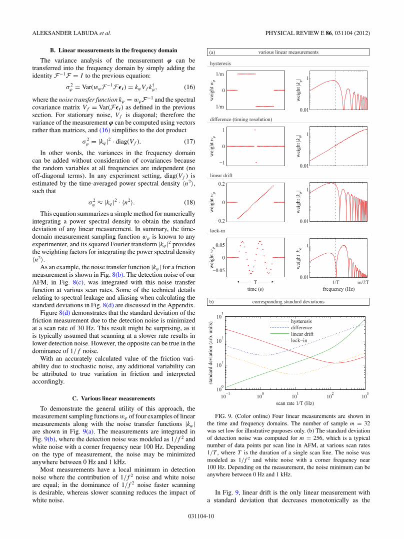
C. Various linear measurements

To demonstrate the general utility of this approach, themeasurement sampling functions wϕ of four examples of linearmeasurements along with the noise transfer functions |kϕ|are shown in Fig. 9(a). The measurements are integrated inFig. 9(b), where the detection noise was modeled as 1/f 2 andwhite noise with a corner frequency near 100 Hz. Dependingon the type of measurement, the noise may be minimizedanywhere between 0 Hz and 1 kHz.

Most measurements have a local minimum in detectionnoise where the contribution of 1/f 2 noise and white noiseare equal; in the dominance of 1/f 2 noise faster scanningis desirable, whereas slower scanning reduces the impact ofwhite noise.

0.01

1

wei

ght|

k|

0

1/m

wei

ght w

0.01

1

−1

0

1

0.01

1

−0.2

0

0.2

0.01

1

frequency (Hz)

−0.05

0

0.05

time (s)

hysteresis

difference (timing resolution)

linear drift

lock-in

1/m

1/T m/2TT

10−1

100

101

102

103

100

101

102

103

scan rate 1/T (Hz)

stan

dard

dev

iati

on (

unit

s)ar

b.

hysteresisdifferencelinear driftlock−in

wei

ght|

k|

wei

ghtw

wei

ght |

k|

wei

ght w

wei

ght|

k|

wei

ght w

ϕ

corresponding standard deviations

various linear measurements

b)

(a)

ϕϕ

ϕ ϕϕ

ϕϕ

FIG. 9. (Color online) Four linear measurements are shown inthe time and frequency domains. The number of sample m = 32was set low for illustrative purposes only. (b) The standard deviationof detection noise was computed for m = 256, which is a typicalnumber of data points per scan line in AFM, at various scan rates1/T , where T is the duration of a single scan line. The noise wasmodeled as 1/f 2 and white noise with a corner frequency near100 Hz. Depending on the measurement, the noise minimum can beanywhere between 0 Hz and 1 kHz.

In Fig. 9, linear drift is the only linear measurement witha standard deviation that decreases monotonically as the

031104-10


scan rate decreases. This decrease occurs because drift is anintrinsically time-dependent quantity: the longer the acquisi-tion, the larger the drift signal becomes. This effect outweighs1/f 2 noise in the case of such time-dependent measurements.

D. Discussion

The data in Fig. 1 were acquired with a difference signal|�0| = 0.007, which allowed us to reconstruct the PSD ofdetection noise by the weighted sum of common-mode anddifferential-mode noise of our SLD, using Eq. (4). Theresulting PSD was integrated using Eq. (18) to provide anaccurate measure of the standard deviation expected fordetection noise in our friction experiment. The calculateddetection noise of 15 pN is just below the measured variabilityof 19 pN in Fig. 1. This implies that the true friction variabilityon gold is barely resolvable above detection noise. On the otherhand, 28 pN of the observed 32 pN of variability on copper isattributed to true changes in friction.

The true variability in friction on copper chloride is distin-guishable from detection noise as it is not white. In fact, it iscloser to brown noise, suggesting that there are slow processesthat cause most of the friction variability. Experiments haveshown 1/f variations in friction due to wear debris [43].Although our experiment is well below the onset of wear,studying the differences in statistical distributions of frictionon a copper chloride monolayer vs gold can help understandthe effects of adsorbed monolayers on nanoscale friction [44].This would provide additional information regarding changesof the tip-sample junction composition, such as rearrangementof the tip atoms or sporadic changes in the ionic compositionnear the surface that may affect the coadsorption of chloridewith the copper monolayer, all of which can contribute tochanges in friction. Furthermore, the distribution of frictioncan be related to the statistics of the stick-slip jump events tounderstand the effects of thermal fluctuations as well as theatomic structure and orientation of the surface on the outcomeof a nanoscale friction experiment [45]. Alas, a reductionin detection noise is required to study the true fluctuationsin friction on copper chloride vs gold and their statisticalproperties in our experiment.

For the data in Fig. 1, our scan rate was set to 25 Hz, whichfalls within the minimum region around 30 Hz as seen inFig. 8(d). This region occurs because of the joint minimizationof 1/f and white noise, as well as the rejection of 60 Hz andharmonics for a scan rate of exactly 30 Hz. Notice that thenoise transfer function |kϕ| of a friction experiment has zerosat even harmonics of the scan rate. At these frequencies, aninteger number of periods fit into the friction measurementsampling function wϕ , and therefore cause zero error in frictionregardless of their amplitude.

It would have been worthwhile to properly center thedetection light beam (|�0| = 0) at the beginning of theexperiment to remove common-mode noise which contributed∼20% of additional detection noise. Any further reduction indetection noise would require design changes to our AFM.The use of softer cantilevers [33] would reduce the detectionnoise of lateral force, which to first order scales linearlywith torsional stiffness. Secondly, the reduction of the lightbeam divergence would also lead to lower detection noise.The light beam divergence can be reduced by using a smaller

collimated light beam diameter, a longer effective focal lengthfor focusing the light beam, exploiting the stress-inducedcantilever radius of curvature [46], or patterning the cantileverwith a diffraction grating [14].

It is instructive to note that boosting the light power, bycoating the cantilever or increasing the SLD drive current,would not reduce the detection noise because the frictiondetection noise is dominated by 1/f noise for scan rates below100 Hz on our system. This occurs because the hysteresisnoise transfer function, seen in Fig. 9(a), has a peak at lowfrequencies around the scan rate, whereas higher-frequencyshot noise is mostly averaged out by the measurement samplingfunction. Increasing optical power only reduces detection shotnoise. Actually, coating the cantilever would only increasethe normal force noise at low frequencies due to couplingbetween optical power fluctuations and cantilever thermallyinduced bending [14].

VII. STOCHASTIC SIMULATION

Certain experiments require simulation, rather than calcu-lation such as performed in the previous section, to quantifythe effects of noise on the outcome of the experiment.Specifically, this is necessary for nonlinear situations, forwhich a linear measurement sampling function does not existand a PSD cannot be simply integrated. In this section, amethod for simulating stochastic Gaussian noise from anyarbitrary spectral distribution is presented, and is used ina friction experiment simulation to quantify the effects ofmechanical vibrations of the AFM on atomic-scale friction.

A. The inverse fast Fourier transform methodfor simulating Gaussian noise

The detailed description of the probability distribution ofpower spectral densities in Sec. V contains the ingredientsfor simulating stochastic Gaussian noise. The true powerspectral density n2 may be approximated by a measured 〈n2〉 orcalculated from a theoretical model. Given an equally spacedm × 1 vector 〈n2〉, a frequency-domain noise vector ε f can besimulated as follows.

The first half of ε f must be drawn from a complexnormal distribution; the real and imaginary elements of εf1/2

for each frequency bin are drawn from independent normaldistributions with mean 0 and variance 〈n2〉/2, as in

εf1/2 = N(

0,〈n2〉

2

)+ iN

(0,

〈n2〉2

). (19)

Then, the ε f must be arranged to comply with the propertiesof a real signal in the time domain [39]: the negative frequen-cies must be complex conjugates of the positive frequencies,such that ε f = [εf1/2ε

∗f1/2

], and ε∗f1/2

must be flipped. Finally, theresulting 2m × 1 vector ε f can be converted to a time-domainnoise vector by the inverse Fourier transform matrix:

εt = F−1ε f , (20)

which can be efficiently computed using the fast Fouriertransform (FFT).

The caveat in using this method is that theF−1 is a circulantmatrix, making the first and last data points of εt contiguous,and therefore strongly correlated. This assumption has no

031104-11


consequence for generating noise with no periodicity orlong-range correlation, such as white noise, for example. Thecirculant property is also relatively inconsequential for anoscillatory signal which decorrelates within the time windowof the generated data set. In any case, the safest approachis to generate 2× more data than requested and to discardhalf of the data. This results in a m × 1 noise vector εt . For1/f noise, which is divergent, it may be necessary to discardmore than half the data to achieve a desired level of statisticalaccuracy, depending on the exponent of the 1/f noise. Thismethod was used to generate the Gaussian noises in Figs. 5and 6 from their PSDs, for example.

B. Simulating displacement noise

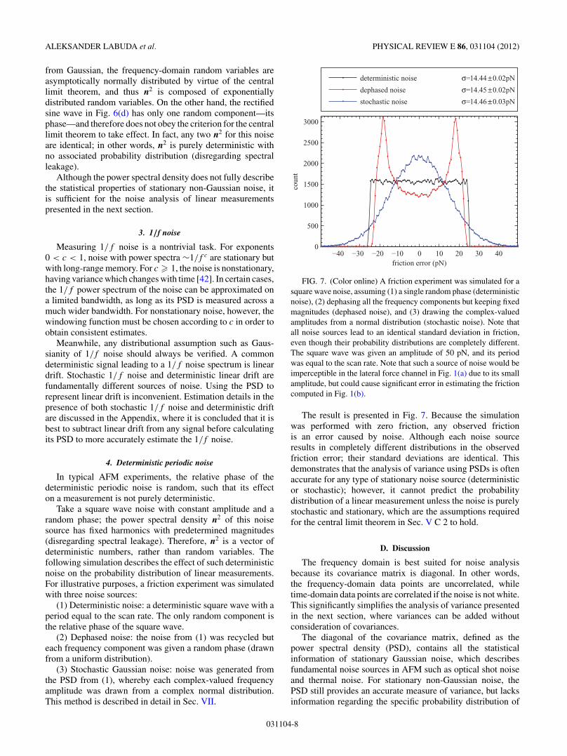
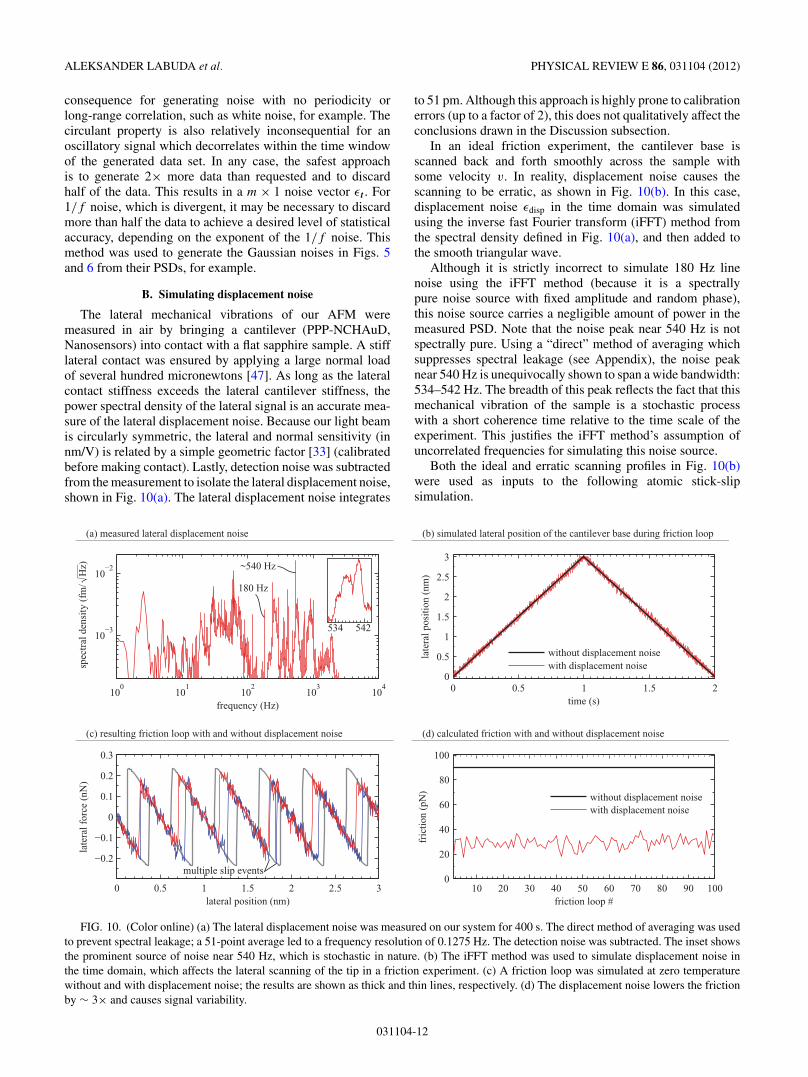
The lateral mechanical vibrations of our AFM weremeasured in air by bringing a cantilever (PPP-NCHAuD,Nanosensors) into contact with a flat sapphire sample. A stifflateral contact was ensured by applying a large normal loadof several hundred micronewtons [47]. As long as the lateralcontact stiffness exceeds the lateral cantilever stiffness, thepower spectral density of the lateral signal is an accurate mea-sure of the lateral displacement noise. Because our light beamis circularly symmetric, the lateral and normal sensitivity (innm/V) is related by a simple geometric factor [33] (calibratedbefore making contact). Lastly, detection noise was subtractedfrom the measurement to isolate the lateral displacement noise,shown in Fig. 10(a). The lateral displacement noise integrates

to 51 pm. Although this approach is highly prone to calibrationerrors (up to a factor of 2), this does not qualitatively affect theconclusions drawn in the Discussion subsection.

In an ideal friction experiment, the cantilever base isscanned back and forth smoothly across the sample withsome velocity v. In reality, displacement noise causes thescanning to be erratic, as shown in Fig. 10(b). In this case,displacement noise εdisp in the time domain was simulatedusing the inverse fast Fourier transform (iFFT) method fromthe spectral density defined in Fig. 10(a), and then added tothe smooth triangular wave.

Although it is strictly incorrect to simulate 180 Hz linenoise using the iFFT method (because it is a spectrallypure noise source with fixed amplitude and random phase),this noise source carries a negligible amount of power in themeasured PSD. Note that the noise peak near 540 Hz is notspectrally pure. Using a “direct” method of averaging whichsuppresses spectral leakage (see Appendix), the noise peaknear 540 Hz is unequivocally shown to span a wide bandwidth:534–542 Hz. The breadth of this peak reflects the fact that thismechanical vibration of the sample is a stochastic processwith a short coherence time relative to the time scale of theexperiment. This justifies the iFFT method’s assumption ofuncorrelated frequencies for simulating this noise source.

Both the ideal and erratic scanning profiles in Fig. 10(b)were used as inputs to the following atomic stick-slipsimulation.

(a) measured lateral displacement noise (b) simulated lateral position of the cantilever base during friction loop

(d) calculated friction with and without displacement noise(c) resulting friction loop with and without displacement noise

0 0.5 1 1.5 20

0.5

1

1.5

2

2.5

3

time (s)

late

ral p

osit

ion

(nm

)

with displacement noisewithout displacement noise

100

101

102

103

104

10−3

10−2

frequency (Hz)

spec

tral

den

sity

(fm

/ H

z)

without displacement noisewith displacement noise

0.5 1 1.5 2 2.5

−0.2

−0.1

0

0.1

0.2

0.3

lateral position (nm)

late

ral f

orce

(nN

)

180 Hz

~540 Hz

multiple slip events

10 20 30 40 50 60 70 80 90 1000

20

40

60

80

100

friction loop #

fric

tion

(pN

)

0 3

534 542

FIG. 10. (Color online) (a) The lateral displacement noise was measured on our system for 400 s. The direct method of averaging was usedto prevent spectral leakage; a 51-point average led to a frequency resolution of 0.1275 Hz. The detection noise was subtracted. The inset showsthe prominent source of noise near 540 Hz, which is stochastic in nature. (b) The iFFT method was used to simulate displacement noise inthe time domain, which affects the lateral scanning of the tip in a friction experiment. (c) A friction loop was simulated at zero temperaturewithout and with displacement noise; the results are shown as thick and thin lines, respectively. (d) The displacement noise lowers the frictionby ∼ 3× and causes signal variability.

031104-12


C. Simulation of atomic stick-slip

This simulation is based on the one-spring Tomlinson model[48], which assumes that the potential Ua(x) in the lateraldirection x is sinusoidal with a period defined by the atomiclattice of the substrate. A time-varying harmonic potential ofthe contact is defined by the effective lateral contact stiffnessk, as in

Uc(x,t) = 12k(x − vt + εdisp)2, (21)

which includes the scanning velocity v and displacement noiseεdisp discussed earlier. At every time step in the simulation, thenew tip position is reassigned as the new local minimum inthe combined potential U = Ua + Uc. This implicitly assumesthat the system temperature is zero. It also conveniently makesthe following simulation purely deterministic, such that theeffects of stochastic displacement noise, simulated in theprevious section, can be isolated unambiguously. To this end,detection noise was also omitted from the simulation.

The parameters used for the simulation were taken from aprevious simulation of atomic stick-slip performed by Socoliucet al. [49]. A tip was scanned at v = 3 nm/s across NaClwith a lattice constant a = 0.5 nm, and an effective lateralcontact stiffness k = 1 N/m. The corrugation energy E0 of thesinusoidal potential was set to 0.237 eV, resulting in η = 3,where η = 2π2E0/ka2. The η parameter defines the stick-slip(η > 1) and the continuous sliding (η < 1) regimes of friction.

By assuming no displacement noise, the simulation resultsin a predictable stick-slip pattern represented by thick graylines in Fig. 10(c). Including displacement noise in thesimulation strongly affects the outcome of the experiment,as shown by the overlaid thin lines in Fig. 10(c). The timingof the slip events has significant variability. Furthermore, themeasured friction force is much lower relative to the idealcase, as summarized by the 100 simulations in Fig. 10(d). Thefriction loops of all 100 simulations are available elsewhere(see Supplemental Material [50]).

D. Discussion

The peak lateral force required to initiate a slip event seemsto have dropped significantly due to displacement noise, asseen by comparing both friction loops in Fig. 10(c). However,this is simply an illusion caused by averaging the data to aneffective 512-Hz sampling rate. On the time scale of eachsimulation step (5 kHz), the lateral force that leads to a slipevent is exactly 0.239 nN by virtue of the assumed Tomlinsonmodel. The displacement noise at high frequencies causes thislateral force threshold to be reached prematurely, resultingin early slip events and a threefold reduction in friction. Thisillustrates the nonlinear nature of this simulation: displacementnoise can cause an early slip event, which is usually irreversiblebecause the cantilever subsequently remains in its new localminimum of the combined potential U . Displacement noisecan also induce back-and-forth slip events, as pointed out inFig. 10(c), where a large stochastic mechanical disturbancecauses the tip to jump back and forth between two latticepositions. Similar events have been observed experimentally[51] and postulated theoretically [52,53]. Lastly, the stochasticnature of the displacement noise also causes significantvariability in friction, as seen in Fig. 10(d). Such variability

would not be observed if dynamic superlubricity were inducedby a deterministic sine wave [31], for example.

The mechanism that causes the suppression of friction de-scribed so far is akin to a thermal activation process describedby Arrhenius transition state theory. Thermal activation of slipevents has been theoretically proposed by Gnecco et al. [48]and Sang et al. [54], and is still under study today [55].Such models predict a decrease in friction with increasingtemperature as well as a logarithmic dependence of frictionwith scanning velocity.

Similarly, stochastic displacement noise can assume a loga-rithmic velocity dependence because the mechanical activationprocess reported here is analogous to thermal activation. ForGaussian displacement noise, the amplitude of the tip-samplevibrations follows a normal distribution, such that the instan-taneous potential energy (amplitude squared) of the systemfollows an exponential distribution. Secondly, the attemptfrequency (the rate parameter in the Arrhenius equation)relates directly to the coherence time of the mechanical noise.

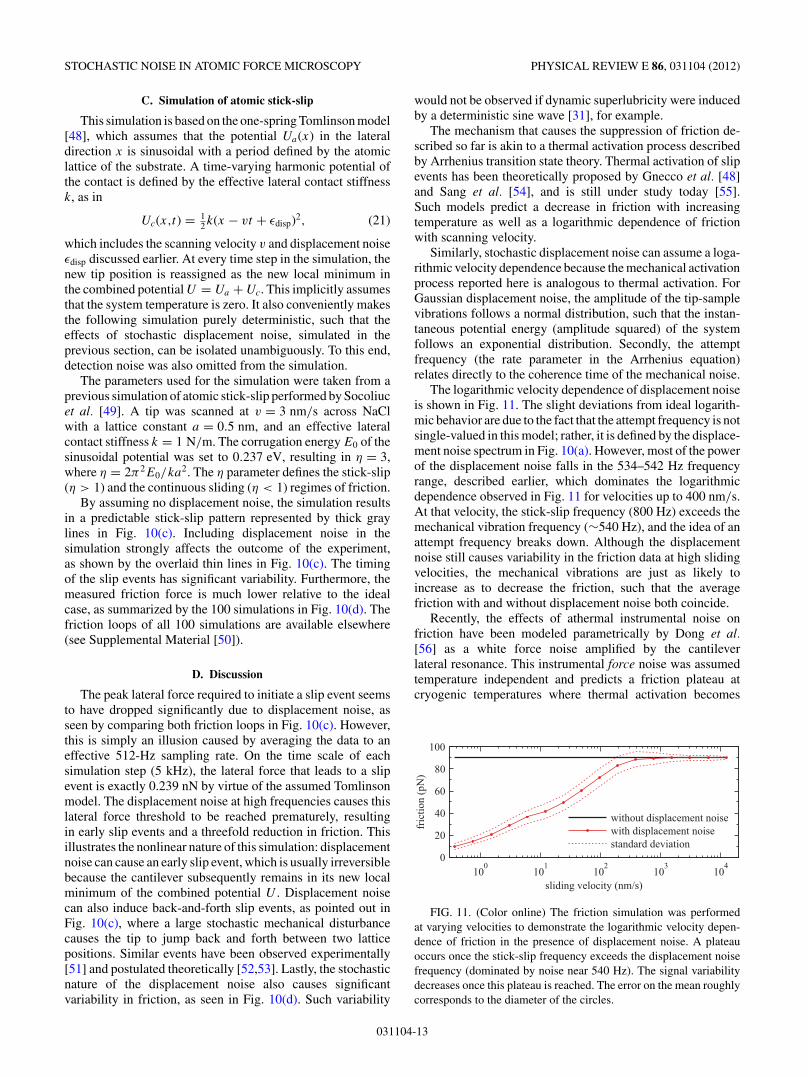
The logarithmic velocity dependence of displacement noiseis shown in Fig. 11. The slight deviations from ideal logarith-mic behavior are due to the fact that the attempt frequency is notsingle-valued in this model; rather, it is defined by the displace-ment noise spectrum in Fig. 10(a). However, most of the powerof the displacement noise falls in the 534–542 Hz frequencyrange, described earlier, which dominates the logarithmicdependence observed in Fig. 11 for velocities up to 400 nm/s.At that velocity, the stick-slip frequency (800 Hz) exceeds themechanical vibration frequency (∼540 Hz), and the idea of anattempt frequency breaks down. Although the displacementnoise still causes variability in the friction data at high slidingvelocities, the mechanical vibrations are just as likely toincrease as to decrease the friction, such that the averagefriction with and without displacement noise both coincide.

Recently, the effects of athermal instrumental noise onfriction have been modeled parametrically by Dong et al.[56] as a white force noise amplified by the cantileverlateral resonance. This instrumental force noise was assumedtemperature independent and predicts a friction plateau atcryogenic temperatures where thermal activation becomes

100

101

102

103

104

0

20

40

60

80

100

sliding velocity (nm/s)

fric

tion

(pN

)

without displacement noisewith displacement noisestandard deviation

FIG. 11. (Color online) The friction simulation was performedat varying velocities to demonstrate the logarithmic velocity depen-dence of friction in the presence of displacement noise. A plateauoccurs once the stick-slip frequency exceeds the displacement noisefrequency (dominated by noise near 540 Hz). The signal variabilitydecreases once this plateau is reached. The error on the mean roughlycorresponds to the diameter of the circles.

031104-13


negligible. In other words, the instrument was assumed to havea finite effective temperature caused by instrumental noise.

In contrast, our simulation uses an empirical measurementof the displacement noise of our instrument as input. Thedynamics of the cantilever play no role in this simulatedexperiment because the lateral resonance frequency of thecantilever, say 150 kHz, greatly exceeds the mechanicalvibrations of the AFM (<3 kHz). In that respect, the cantilevercan be accurately described as an ideal force sensor that doesnot affect the outcome of the experiment. Nevertheless, thedisplacement noise can be attributed a cantilever-equivalenteffective temperature. By the equipartition theorem, thecantilever in this simulation is expected to have 12 pm ofvibrational noise at room temperature (

√kBT /kc), while there

is 51 pm of integrated displacement noise (across the 1 Hz to10 kHz bandwidth). In other words, the cantilever temperaturewould have to be 5500 K for the integrated cantilever noise toexceed the integrated displacement noise.

We now note the problematic fact that the displacementnoise of an AFM is expected to be temperature dependent.The mechanical response of an AFM has been shown to changedrastically at cryogenic temperatures [57]. Due to the lowereddamping of hardware components in the AFM, the externalnoise coupling drives the mechanical components with largeramplitudes and can promote the suppression of friction atcryogenic temperatures. This may result in a nonmonotonictemperature dependence of friction that would be characterizedby a drop in friction at low temperatures.

We conclude that the reduction of friction by mechanicaldithering of the sample, known as dynamic superlubricity [31],inadvertently occurs due to inevitable mechanical vibrationsof an AFM. The degree of this friction suppression dependson a multitude of experimental parameters and the specificdisplacement noise of the AFM in question. Therefore, ageneral quantitative assessment of the problem cannot bemade. However, the method proposed here can be used toestimate the expected impact of displacement noise on anyparticular system and experiment. Measuring the temperaturedependence of the displacement noise is also recommendedbefore performing an experiment for studying the temperaturedependence of friction.

VIII. SUMMARY AND CONCLUSIONS

The power spectral density (PSD) of detection noise maychange during an experiment if the light beam does notremain perfectly centered on the photodetector. This PSD ismeasurable and predictable after characterizing the common-mode and differential-mode noise of the light beam used tomeasure the cantilever deflections.

An intuitive method for integrating a PSD to provideaccurate estimates of any linear measurement was presented,allowing predictive power over experiments, and informedanalysis of measured data. We have shown that the variabilityin measured friction may be dominated by detection noise evenin situations with clearly resolved stick-slip. Interestingly,increasing the light power (by a reflective coating, for example)does not reduce this friction variability, which is limited by1/f angular noise of the light beam. In the dominance of1/f noise, faster scanning reduces the impact of noise on the

measurement. From a noise analysis perspective, the optimalscan rate for friction experiments is 30 Hz, on our particularAFM.

The power spectral density is a powerful tool for noiseanalysis of stationary noise, either stochastic or deterministic.Understanding the statistical properties of measured PSDs fordifferent noise sources provides the necessary foundation forthe simulation of AFM experiments affected by stochasticnoise. Such simulations allow the assessment of the relativecontribution of detection, force, and displacement noisesources in any particular AFM experiment.

In this work, stochastic simulation of measured displace-ment noise was used to quantify the effects of mechanicalvibrations on the outcome of a friction experiment. Assuming aone-spring Tomlinson model with typical scanning conditionsand zero temperature, our simulation predicts that the dis-placement noise can cause a logarithmic velocity dependenceof friction, induce multiple back-and-forth slip events in theatomic stick-slip process, and cause significant variability inmeasured friction.

An attractive feature of the iFFT method of stochasticsimulation is that it is not restricted to parametric models:any arbitrary numerically defined PSD can be used as input.Mechanical vibrations between the tip and the sample, forexample, can only be empirically measured, and may bedifficult to accurately or efficiently describe parametrically.We have attributed a stochastic sample vibration near 540 Hzas the largest contributor to athermal friction suppression andincreased friction variability on our system.

Although we have demonstrated noise analysis and stochas-tic simulations in the context of friction experiments, thesemethods can be used for a wide range of AFM experiments, andextend to dynamic AFM measurements as well [58]. Stochasticsimulations can be used for the optimization of experimentalprotocols by aiding in the selection of experimental param-eters. Tandem simulations can also be used alongside actualexperiments to diagnose the cause of variability, and to assesswhether a measurement is limited by fundamental sources ofnoise, mechanical vibrations, or simply due to true variabilityof the physical system being measured.

ACKNOWLEDGMENTS

We acknowledge valuable discussions with Philip Egbertsand Jason Cleveland, and funding from NSERC and FQRNT.

APPENDIX

This Appendix outlines certain technical details regardingthe integration of PSDs, as well as their estimation usingFourier transform methods. Before proceeding, the readershould be familiar with the concepts of “spectral leakage”and “aliasing,” described in the following paragraphs.

Spectral leakage occurs because a perfect sine wave(infinitely long in time) cannot be measured in practice: itis inevitable that its measurement is performed within a finitetime window. Truncating a perfect sine wave introduces newfrequency components into the measurement. In other words,the power of the single frequency sine wave “leaks” into

031104-14


adjacent frequencies. This description generalizes to signalsof any arbitrary shape.

Aliasing is due to the finite-time sampling of a signal. Thiseffect causes familiar phenomena such as the appearance of carwheels rotating backwards in films, for example. Similarly, insignal processing, slowly sampling a fast signal “aliases” fastfrequencies onto slower ones. For a sampling rate of 100 Hz,different sine waves at 10, 90, 110, 190, 210 Hz, etc., all appearidentical and indistinguishable from a 10-Hz sine wave.

1. Numerical details for PSD integration

In order to numerically integrate an average power spectraldensity 〈n2〉 weighted by a noise transfer function |kϕ|, bothvectors must share an identical frequency basis. Typically, thesystem noise is characterized before the experiment over alarge frequency range such as 10−2–106 Hz, which is muchwider than the experiment bandwidth of, say, 100–103 Hz.However, noise at frequencies below and above the experimentbandwidth affect the measurement by the mechanisms ofspectral leakage and aliasing, respectively.

We use zero-padding and zero-interleaving in the timedomain as methods for extending the frequency range of |kϕ| tomatch the frequency range of 〈n2〉 for an accurate integrationof the entire frequency spectrum.

Before performing the Fourier transform on the measure-ment sampling function wϕ to obtain |kϕ|, zero-padding shouldbe adjusted to match the frequency resolution of |kϕ| tothe frequency resolution of 〈n2〉, as illustrated in Fig. 12.Zero-padding takes into account the effects of spectral leakageon the measurement.

FIG. 12. (Color online) The sampling function wϕ of a hysteresismeasurement is shown. The number of data points was selectedas m = 16 for plotting purposes only. Zero-padding the signalincreases the frequency resolution and zero-interleaving increasesthe maximum frequency. The creation of Nyquist zones above thesampling frequency simulates aliasing. Both are tuned such that thefrequency basis of the noise transfer function |kϕ | corresponds to themeasured detection noise 〈n2〉. The |kϕ | here is shown for m = 256in the second plot, for a scan rate of 10 Hz.

Next, zero-interleaving is used to increase the maximumfrequency of |kϕ| beyond the roll-off frequency of 〈n2〉.Zero-interleaving takes into account the effects of aliasingduring analog-to-digital conversion, by extending |kϕ| tohigher frequencies. Every zero that is interleaved generatesa new Nyquist zone, as shown in Fig 8(b). Typical ADCshave a fixed integration time per sample, such that loweringthe sampling rate from its maximum causes “dead time” inbetween samples leading to aliasing; this process is mimickedby zero-interleaving as illustrated by Fig. 12(a). Note thatthe peaks for each Nyquist zone indicate the unnecessaryand undesirable aliasing of high-frequency noise into themeasurement. Two methods can be used to reduce aliasing:(1) oversampling the signal by operating the ADC at itsmaximum sampling rate removes the Nyquist zones as allthe high-frequency noise is measured and averaged by themeasurement sampling function; (2) low-pass filtering thesignal (prior to sampling) at a frequency below the Nyquistfrequency (fs/2), such that no noise remains in the Nyquistzones. Both of these methods prevent high-frequency noisefrom aliasing into the measurement bandwidth.

The Fourier transform of the zero-padded and zero-interleaved sampling function is shown in Fig. 12, overlaid onthe detection noise. In practice, the matching of both frequencybases cannot be achieved perfectly, such that appropriateinterpolation is used as a final step. Finally, the variance of themeasurement can be computed by the dot product: |kϕ|2 · 〈n2〉.

2. Accurate PSD estimation

The covariance matrix Vf is experimentally estimated bythe average power spectral density vector 〈n2〉. The accuracyof this estimation is mainly limited by spectral leakage, drift,and statistical biases, which are the topics of this section.

a. Spectral leakage and windowing. Omitting windowingduring the Fourier transform (i.e., using a rectangular window)causes biases when estimating 1/f noise due to spectralleakage. For example, a 2× bias in the estimation of 1/f 2

noise occurs because the rectangular window falls off with1/f 2 itself; convoluting a 1/f 2 noise with a 1/f 2 windowresults in 2/f 2. Furthermore, spectral leakage correlatesadjacent frequencies of a spectral density, thereby violating theassumption of a diagonal spectral covariance matrix presentedin Eq. (9). This section presents a method for reducing theeffects of spectral leakage compared to traditional methodsused for calculating 〈n2〉 from a time series.

Bartlett’s method [59] for power spectral density estimationamounts to dividing a time series into smaller segments,calculating their respective spectral densities, and averagingthem. This reduces the variance of the 〈n2〉 estimation, atthe expense of reducing the frequency resolution. Spectralleakage in this situation becomes much more problematic,because the duration of each time series is much shorter.Welch’s method [60] offsets this problem to a certain extent,by windowing each time series. This reduces the effects ofthe time-window edge discontinuities of each time series.However, significant spectral leakage still occurs regardlessof the windowing function that is used.

Arguably, the main advantage of these two methods isthe reduction in necessary computing power, which was

031104-15


FIG. 13. The same simulated noise data were used for all threepower spectral density estimations. The line noise peaks (60, 120,180 Hz) were modeled as perfect sine waves with an arbitrary phase.(a) The Welch method causes estimation bias at low frequencies (1)and spectral leakage (2). (b) The direct method solves these problems,but the increase in variance at high frequencies (3) remains illusory.Also, the bandwidth of noise peaks can become thinner than thegraphical linewidth of 0.176 mm (4), thereby distorting the perceptionof the power of each noise source. (c) These problems are solvedusing logarithmic averaging. All methods used a Hann window whencomputing the Fourier transform.

scarce in the 1960s when these methods were developed.The availability of modern computing led us to adopt amore simple and direct method of PSD estimation for whichspectral leakage can mostly be eliminated: a single PSD of theentire time series is calculated (after appropriate windowing)followed by averaging groups of adjacent frequency bins toreduce the variance [61]. The same trade-off between varianceand resolution remains, but spectral leakage can be tunedarbitrarily small and the estimation bias at low frequenciesis prevented. This is illustrated in Figs. 13(a) and 13(b), whereWelch’s method is contrasted with the “direct method.”

Figure 13(c) uses the same data as Fig. 13(b) whichwere subsequently averaged using logarithmically spacedfrequency bins, making it more suitable for plotting on alogarithmic scale. Basically, for a linearly spaced PSD inthe frequency range [a,b], the N -sized logarithmically spacedPSD is generated by grouping all data points that fall withinthe frequency range [ae(i−1)ln(b/a)/N ,aeiln(b/a)/N ], where i is thebin index from 1 to N .

This presents a quantitatively more accurate visual repre-sentation of the power spectral density for applications wherea logarithmic frequency axis is more appropriate, such as staticAFM. In reality, the variance of shot noise decreases towardsthe right of a logarithmic graph where there are many moredata points which estimate shot noise for a given fractionalbandwidth �ω/ω. (Note that in certain applications, such asdynamic AFM, the figure of merit is the linear bandwidth �ω

in which case logarithmic averaging is not appropriate.)Also, certain noise peaks appear significant in Fig. 13(b),

but should be disregarded because their bandwidth is verysmall and therefore the corresponding power is insignificant;for example, of the two peaks labeled (4) that appear identicalin Fig. 13(b), the one to the right has a bandwidth that is 30×smaller, which is apparent by inspection of the graph plotted inFig. 13(c). We stress that logarithmic averaging in Fig. 13(c)is used only for visual representation of PSDs, whereas thedirect method is used in noise analysis as it contains moreinformation.

b. 1/f noise vs drift. As a disclaimer, it should be notedthat the distinction between drift and 1/f noise is the topicof debate, and the discussion presented herein is based on theassumption that drift is caused by a deterministic process,while 1/f noise is inherently stochastic. As described inSec. V A, the distinction between stochastic and deterministicnoise can be a matter of perspective.

Although 1/f noise and drift can be difficult to distinguishexperimentally [62], they require different treatment. Forexample, the average PSDs of both linear drift and Brownianmotion converge to a 1/f 2 power spectrum. Brownian motionis a stochastic process, with a zero mean, and the PSDcorrectly estimates its variance (assuming spectral leakage isappropriately handled). In contrast, drift can be thought ofas a deterministic process on the short time scale of a singleexperiment. Drift has a predictable effect on the mean (ratherthan variance) of a signal, and therefore is not accuratelydescribed by a PSD.

Properly quantifying the variability of drift itself wouldrequire a PSD measurement taken across many days, and astrong component is expected at a frequency of day−1 becausetemperature cycles between day and night are prominent.In fact, the 1/f 2 power spectrum of linear drift at shorterexperimental time scales is simply a result of spectral leakage:the long time scale drift oscillations are truncated by a finitetime window, and the edge effects of this truncation resultin spectral leakage. The 1/f 2 power spectrum of linear driftrelates only to the rectangular windowing function, and canbe changed to 1/f 8 simply by choosing a Hann windowingfunction, for example. Furthermore, a PSD of any finite signalis equivalent to the PSD of an infinite periodic signal; the PSDof linear drift is equivalent to the PSD of an infinite sawtoothwave. The 1/f 2 spectrum quantifies the harmonics of thatsawtooth wave, which is clearly an incorrect representationof linear drift. In summary, the observed spectrum of drift issimply an artifact of the finite Fourier transform method, andits shape provides no information about the actual drift.

For these reasons, drift must be subtracted from any signalbefore taking its PSD. It is inevitable that any estimate ofdrift (to be subtracted) will be corrupted by 1/f noise, andconversely the measurement of 1/f noise will be altered

031104-16


by the drift subtraction. For short experiments, a simplelinear drift can be a very good approximation, while longerexperiments may require the subtraction of nonlinear drift thatmay be modeled as polynomial drift, or logarithmic creep, forexample. All the PSDs reported in this paper were calculatedafter subtraction of a linear drift, judging that the remainingnoise can accurately be described as “variance” on the timescales considered.

c. Amplitude averaging. The amplitude spectral density |n|rather than the power spectral density |n|2 is often used innoise analysis. As derived in Sec. IV, each random variable in

|n|2 is exponentially distributed, implying that each randomvariable in |n| follows a Rayleigh distribution. Squaring andaveraging are noncommutative operations: 〈|n|2〉 = 〈|n|〉2 (theaverage of the squares is not the square of the average).However, the two relate by a calculable statistical bias, andthe average power spectral density of stochastic noise canbe determined from the average amplitude spectral densityby

〈|n|2〉 = 4

π〈|n|〉2. (A1)

[1] G. Binnig, C. F. Quate, and C. Gerber, Phys. Rev. Lett. 56, 930(1986).

[2] Y. Martin, C. C. Williams, and H. K. Wickramasinghe, J. Appl.Phys. 61, 4723 (1987).

[3] T. R. Albrecht, P. Grutter, D. Horne, and D. Rugar, J. Appl. Phys.69, 668 (1991).

[4] S. D. Bennett, L. Cockins, Y. Miyahara, P. Grutter, and A. A.Clerk, Phys. Rev. Lett. 104, 017203 (2010).

[5] J. P. Cleveland, T. E. Schaffer, and P. K. Hansma, Phys. Rev. B52, R8692 (1995).

[6] A. Roters, M. Gelbert, M. Schimmel, J. Ruhe, and D. Johanns-mann, Phys. Rev. E 56, 3256 (1997).

[7] S. Kawai, F. F. Canova, T. Glatzel, A. S. Foster, and E. Meyer,Phys. Rev. B 84, 115415 (2011).

[8] A. Gannepalli, A. Sebastian, J. Cleveland, and M. Salapaka,Appl. Phys. Lett. 87, 111901 (2005).

[9] C. L. Degen, M. Poggio, H. J. Mamin, and D. Rugar, Phys. Rev.Lett. 99, 250601 (2007).

[10] L. Nony, A. Baratoff, D. Schar, O. Pfeiffer, A. Wetzel, andE. Meyer, Phys. Rev. B 74, 235439 (2006).

[11] M. Gauthier, R. Perez, T. Arai, M. Tomitori, and M. Tsukada,Phys. Rev. Lett. 89, 146104 (2002).

[12] J. Melcher, C. Carrasco, X. Xu, J. L. Carrascosa, J. Gomez-Herrero, P. Jose de Pablo, and A. Raman, Proc. Natl. Acad. Sci.USA 106, 13655 (2009).

[13] D. Kiracofe, J. Melcher, and A. Raman, Rev. Sci. Instrum. 83,013702 (2012).

[14] A. Labuda, J. R. Bates, and P. H. Grutter, Nanotechnology 23,025503 (2012).

[15] G. Meyer and N. M. Amer, Appl. Phys. Lett. 53, 1045 (1988).[16] T. Fukuma, T. Ichii, K. Kobayashi, H. Yamada, and

K. Matsushige, Appl. Phys. Lett. 86, 034101 (2005).[17] F. N. Hooge, T. G. M. Kleinpenning, and L. K. J. Vandamme,

Rep. Prog. Phys. 44, 479 (1981).[18] P. Bak, C. Tang, and K. Wiesenfeld, Phys. Rev. Lett. 59, 381

(1987).[19] Y. Sang, M. Dube, and M. Grant, Phys. Rev. E 77, 036123

(2008).[20] C. Zener, Phys. Rev. 52, 230 (1937).[21] V. T. Srikar and S. D. Senturia, J. Microelectromech. Syst. 11,

499 (2002).[22] S. Prabhakar and S. Vengallatore, J. Micromech. Microeng. 17,

532 (2007).[23] J. E. Sader, J. Appl. Phys. 84, 64 (1998).

[24] S. Rast, C. Wattinger, U. Gysin, and E. Meyer, Nanotechnology11, 169 (2000).

[25] M. T. Clark, J. E. Sader, J. P. Cleveland, and M. R. Paul, Phys.Rev. E 81, 046306 (2010).

[26] A. Labuda and P. Grutter, Langmuir 28, 5319 (2012).[27] P. Paolino and L. Bellon, Nanotechnology 20, 405705 (2009).[28] J. B. Thompson, B. Drake, J. H. Kindt, J. Hoskins, and P. K.

Hansma, Nanotechnology 12, 394 (2001).[29] R. Guerra, A. Vanossi, and M. Urbakh, Phys. Rev. E 78, 036110

(2008).[30] A. Socoliuc, E. Gnecco, S. Maier, O. Pfeiffer, A. Baratoff,

R. Bennewitz, and E. Meyer, Science (NY) 313, 207 (2006).[31] M. Lantz, D. Wiesmann, and B. Gotsmann, Nat. Nanotechnol.

4, 586 (2009).[32] C. M. Mate, G. M. McClelland, R. Erlandsson, and S. Chiang,

Phys. Rev. Lett. 59, 1942 (1987).[33] A. Labuda, W. Paul, B. Pietrobon, R. B. Lennox, P. H. Grutter,

and R. Bennewitz, Rev. Sci. Instrum. 81, 083701 (2010).[34] A. Labuda, F. Hausen, N. N. Gosvami, P. H. Grutter, R. B.

Lennox, and R. Bennewitz, Langmuir 27, 2561 (2011).[35] A. Labuda, K. Kobayashi, Y. Miyahara, and P. Grutter, Rev. Sci.

Instrum. 83, 053703 (2012).[36] T. Fukuma, M. Kimura, K. Kobayashi, K. Matsushige, and H.

Yamada, Rev. Sci. Instrum. 76, 053704 (2005).[37] A. Garcıia-Valenzuela and J. Villatoro, J. Appl. Phys. 84, 58

(1998).[38] M. B. Viani, T. E. Schaffer, A. Chand, M. Rief, H. E. Gaub, and

P. K. Hansma, J. Appl. Phys. 86, 2258 (1999).[39] P. Brockwell and R. Davis, Time Series: Theory and Methods,

2nd ed. (Springer, New York, 1991).[40] E. Milotti, Phys. Rev. E 51, 3087 (1995).[41] S. F. Nørrelykke and H. Flyvbjerg, Rev. Sci. Instrum. 81, 075103

(2010).[42] J. Brophy, Phys. Rev. 166, 827 (1968).[43] I. Vragovic, J. M. Molina, R. Prieto, M. Duarte, J. Narciso, and

E. Louis, Phys. Rev. E 80, 066123 (2009).[44] S. Cheng, B. Luan, and M. O. Robbins, Phys. Rev. E 81, 016102

(2010).[45] A. Schirmeisen and H. Holscher, Phys. Rev. B 72, 045431

(2005).[46] A. Labuda and P. H. Grutter, Rev. Sci. Instrum. 82, 013704

(2011).[47] R. W. Carpick, D. F. Ogletree, and M. Salmeron, Appl. Phys.

Lett. 70, 1996 (1997).

031104-17

http://dx.doi.org/10.1103/PhysRevLett.56.930


http://dx.doi.org/10.1063/1.338807

http://dx.doi.org/10.1063/1.338807

http://dx.doi.org/10.1063/1.347347

http://dx.doi.org/10.1063/1.347347


http://dx.doi.org/10.1103/PhysRevB.52.R8692

http://dx.doi.org/10.1103/PhysRevB.52.R8692


http://dx.doi.org/10.1103/PhysRevB.84.115415

http://dx.doi.org/10.1063/1.2037197





http://dx.doi.org/10.1073/pnas.0902240106

http://dx.doi.org/10.1073/pnas.0902240106

http://dx.doi.org/10.1063/1.3669638

http://dx.doi.org/10.1063/1.3669638

http://dx.doi.org/10.1088/0957-4484/23/2/025503

http://dx.doi.org/10.1088/0957-4484/23/2/025503

http://dx.doi.org/10.1063/1.100061

http://dx.doi.org/10.1063/1.1850186

http://dx.doi.org/10.1088/0034-4885/44/5/001





http://dx.doi.org/10.1103/PhysRev.52.230

http://dx.doi.org/10.1109/JMEMS.2002.802902

http://dx.doi.org/10.1109/JMEMS.2002.802902

http://dx.doi.org/10.1088/0960-1317/17/3/016

http://dx.doi.org/10.1088/0960-1317/17/3/016

http://dx.doi.org/10.1063/1.368002

http://dx.doi.org/10.1088/0957-4484/11/3/306

http://dx.doi.org/10.1088/0957-4484/11/3/306



http://dx.doi.org/10.1021/la300557u

http://dx.doi.org/10.1088/0957-4484/20/40/405705

http://dx.doi.org/10.1088/0957-4484/12/3/331



http://dx.doi.org/10.1038/nnano.2009.199




http://dx.doi.org/10.1063/1.3470107

http://dx.doi.org/10.1021/la104497t

http://dx.doi.org/10.1063/1.4712286

http://dx.doi.org/10.1063/1.4712286

http://dx.doi.org/10.1063/1.1896938

http://dx.doi.org/10.1063/1.368001

http://dx.doi.org/10.1063/1.368001

http://dx.doi.org/10.1063/1.371039


http://dx.doi.org/10.1063/1.3455217

http://dx.doi.org/10.1063/1.3455217

http://dx.doi.org/10.1103/PhysRev.166.827






http://dx.doi.org/10.1063/1.3503220

http://dx.doi.org/10.1063/1.3503220


[48] E. Gnecco, R. Bennewitz, T. Gyalog, C. Loppacher,M. Bammerlin, E. Meyer, and H. J. Guntherodt, Phys. Rev.Lett. 84, 1172 (2000).

[49] A. Socoliuc, R. Bennewitz, E. Gnecco, and E. Meyer, Phys. Rev.Lett. 92, 134301 (2004).

[50] See Supplemental Material at http://link.aps.org/supplemental/10.1103/PhysRevE.86.031104 for 100 simulated friction loops.

[51] S. Maier, Y. Sang, T. Filleter, M. Grant, R. Bennewitz, E. Gnecco,and E. Meyer, Phys. Rev. B 72, 245418 (2005).

[52] S. Y. Krylov and J. W. M. Frenken, J. Phys. Condens. Matter 20,354003 (2008).

[53] Y. Dong, A. Vadakkepatt, and A. Martini, Tribol. Lett. 44, 367(2011).

[54] Y. Sang, M. Dube, and M. Grant, Phys. Rev. Lett. 87, 174301(2001).

[55] M. H. Muser, Phys. Rev. B 84, 125419 (2011).[56] Y. Dong, H. Gao, and A. Martini, Europhys. Lett. 98, 16002

(2012).[57] A. Labuda, Y. Miyahara, L. Cockins, and P. H. Grutter, Phys.

Rev. B 84, 125433 (2011).[58] A. Labuda, M. Lysy, and P. Grutter, Appl. Phys. Lett. (in press).[59] M. S. Bartlett, Nature 161, 686 (1948).[60] P. Welch, IEEE Trans. Audio Electroacoust. 15, 70 (1967).[61] P. J. Daniell, J. R. Stat. Soc., Ser. B 8, 88 (1946).[62] T. Brettschneider, G. Volpe, L. Helden, J. Wehr, and

C. Bechinger, Phys. Rev. E 83, 041113 (2011).

031104-18





http://link.aps.org/supplemental/10.1103/PhysRevE.86.031104

http://link.aps.org/supplemental/10.1103/PhysRevE.86.031104


http://dx.doi.org/10.1088/0953-8984/20/35/354003

http://dx.doi.org/10.1088/0953-8984/20/35/354003

http://dx.doi.org/10.1007/s11249-011-9850-2

http://dx.doi.org/10.1007/s11249-011-9850-2




http://dx.doi.org/10.1209/0295-5075/98/16002

http://dx.doi.org/10.1209/0295-5075/98/16002



http://dx.doi.org/10.1038/161686a0

http://dx.doi.org/10.1109/TAU.1967.1161901


stochastic noise in atomic force microscopy€¦ · physical review e 86, 031104 (2012) stochastic...

Documents