(stochastic) optimal control : state x, control (dynamic...
TRANSCRIPT

(Stochastic) Optimal Control : State x, Control u (Dynamic Programming)
Stochastic Programming: Variables (x, u), State: dξ − Tξx
Tuesday, June 26, 2012
STOCHASTIC DYNAMIC OPTIMIZATION: APPROACHES AND COMPUTATIONPravin Varaiya and Roger J-B WetsUniversity of California, Berkeley-DavisIn: ``Mathematical Programming, Recent Developments and Applications’’, M. Iri & K. Tanabe (eds), Kluwer Academic Publisher, 1989. pp. 309-332.
(Stochastic) Optimal Control : State x, Control u (Dynamic Programming)
Stochastic Programming: Variables (x, u), State: dξ − Tξx
Tuesday, June 26, 2012

Lectures PlanWhy and how to deal with ‘uncertainty’ (1)
Recourse Models (2 & 3)
Aggregation Principle (4)
Approximations (5)
Duality Theory (6)
Dispatching Energy - ISO (7)
Tuesday, June 26, 2012
Stochastic Programswith Recourse
Roger J-B WetsMathematics, University of California, Davis
Tuesday, June 26, 2012

.. with Simple Recourse
⇒ explicit sol’n
decision: x � observation: ξ � recourse cost evaluation.cost evaluation ‘simple’ ⇒ simple recourse, i.e.,
minx∈S⊂ n f0(x) + {Q(ξ, x)} Q ’simple’
Product mix problem. With ξ = (T, d),f0(x) = �c, x�, S = 4
+, Q(ξ, x) =�
i=c,f max [ 0, γi(�Ti, x� − di) ]
NewsVendor: cost: γ, sale price δ,ξ, demand distribution P , order x,expected “loss”: γx+ {Q(ξ, x)}Q(ξ, x) = −δ · min{x, ξ}
Tuesday, June 26, 2012

Magnet Alignment Imagnets
measumentpoint
Tuesday, June 26, 2012
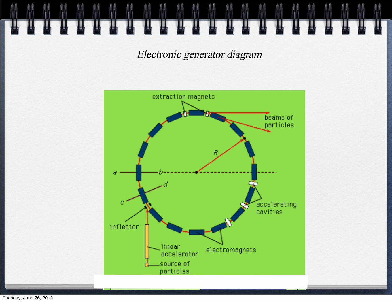
Electronic generator diagram
Tuesday, June 26, 2012
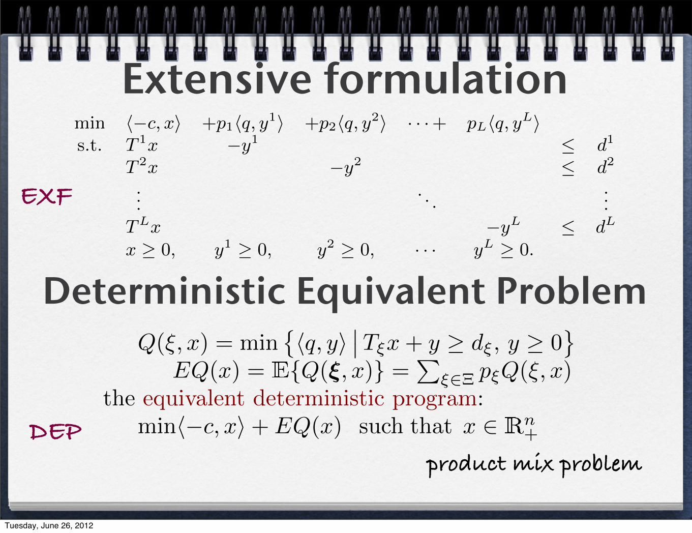
Extensive formulationmin �−c, x� +p1�q, y1� +p2�q, y2� · · ·+ pL�q, yL�s.t. T 1x −y1 ≤ d1
T 2x −y2 ≤ d2
.... . .
...TLx −yL ≤ dL
x ≥ 0, y1 ≥ 0, y2 ≥ 0, · · · yL ≥ 0.
Deterministic Equivalent ProblemQ(ξ, x) = min
��q, y�
��Tξx+ y ≥ dξ, y ≥ 0�
EQ(x) = {Q(ξ, x)} =�
ξ∈Ξ pξQ(ξ, x)the equivalent deterministic program:
min�−c, x�+ EQ(x) such that x ∈ n+
EXF
DEPproduct mix problem
Tuesday, June 26, 2012

Closed Loop vs Open LoopClosed Loop:Observation of state s → control function u(s) (optimal ±)∀s.Stochastic Optimal Control: state s(ξt), control function u(s( ξ
→t))
Hopefully, u( · ) is simple, manageable, . . . , (maybe) time continuous
Open Loop:
Observation of state s → control function u(s) (optimal ±)∀s.Decision Process: from state s(ξt) to decision u(s( ξ
→t))
usually no ‘closed form’ expression
may involve solving an optim. problem
essentially ‘closed loop’ if decision occurs at t+∆t, ∆t small
Tuesday, June 26, 2012

RHS: random right-hand sidesdeterministic version:
min �c, x� such that Ax = b, Tx = ξ, x ≥ 0
stochastic program with simple recourse RHS:
minx �c, x�+�Q(ξ, x)
�such that Ax = b, x ≥ 0
Deterministic Equivalent Problem:
minx �c, x�+ EQ(x) such that Ax = b, x ≥ 0
• f0 = �c, x� is linear;• S =
�x ∈ n
+
��Ax = b�is a polyhedral set, A is m1 × n;
• Q(ξ, x) = q(ξ − Tx), T a non-random m2 × n matrix;• the recourse cost function q : m2 → is convex;• the expectation functional EQ(x) =
�Ξq(ξ − Tx)P (dξ).
(SPwSR)
Tuesday, June 26, 2012

Convex optim., linear constraintsP: f0 : n → convex, X polyhedral,
min f0(x), x ∈ X ⊂ n
such that �Ai, x� ≥ bi, i = 1, . . . , s,
�Ai, x� = bi, i = s+ 1, . . . ,m,
x∗ is an optimal solution of (P) ⇐⇒ ∃, KKT-multipliers y ∈ m:(a) �Ai, x∗� ≥ bi, i = 1, . . . , s, �Ai, x∗� = bi, i = s+ 1, . . . ,m,(b) for i = 1, . . . , s: yi ≥ 0, yi(�Ai, x∗� − bi) = 0,(c) x∗ ∈ argmin
�f0(x)− �A�y, x�
��x ∈ X�.
∼ version of (c): ∃ −v ∈ NX(x∗) =�u�� �u, x− x∗� ≤ 0, ∀x ∈ X
�
Tuesday, June 26, 2012

Optimality: Simple RecourseSuppose EQ finite-valued, x∗ solves SP-simple recourse
⇐⇒ one can find KKT-multipliers u ∈ m1
& summable KKT-multipliers v : Ξ → m2 :
1. x∗ ≥ 0, Ax∗ = b;
2. for all ξ ∈ Ξ: v(ξ) ∈ ∂q(ξ − Tx∗);
3. x∗ ∈ argmin��c−A�u− T�v, x�
��x ∈ n+
�
where v = E{v(ξ)}.
(SPwSR)
Tuesday, June 26, 2012

Reformulation: ... with TendersChange of variables (tenders): χ = Tx
minx,χ �c, x�+ {ψ(ξ,χ)} s.t. Ax = b, Tx = χ, x ≥ 0ψ(ξ,χ) = q(ξ − χ), with Eψ(χ) =
�Ξ ψ(ξ,χ)P (dξ)
Deterministic equivalent problem:minx,χ �c, x�+ Eψ(χ) s.t. Ax = b, Tx− χ = 0, x ≥ 0
Eψ & EQ same properties & ∂Eψ(χ) = − {∂q(ξ − χ)}Usually, ψ, Eψ, are separable while EQ is not,
ψ(ξ,χ) =�m2
i=1 ψi(ξi,χi),=�m2
i=1 qi(ξi − χi)Eψ(χ) =
�m2
i=1 Eψi(χi)
Tuesday, June 26, 2012
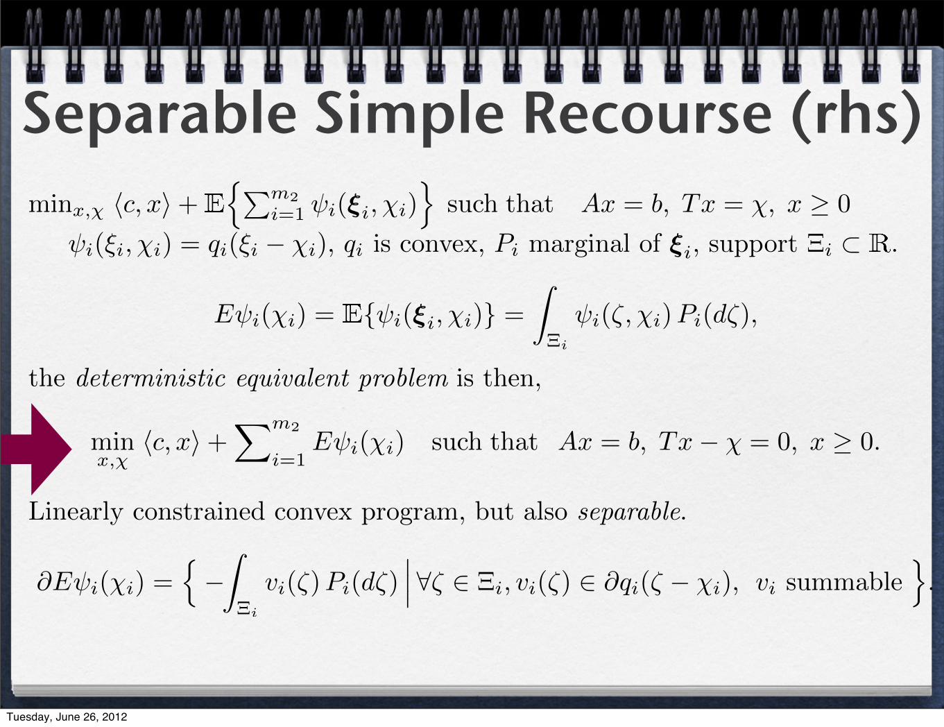
Separable Simple Recourse (rhs)minx,χ �c, x�+
��m2
i=1 ψi(ξi,χi)�
such that Ax = b, Tx = χ, x ≥ 0
ψi(ξi,χi) = qi(ξi − χi), qi is convex, Pi marginal of ξi, support Ξi ⊂ .
Eψi(χi) = {ψi(ξi,χi)} =
�
Ξi
ψi(ζ,χi)Pi(dζ),
the deterministic equivalent problem is then,
minx,χ
�c, x�+�m2
i=1Eψi(χi) such that Ax = b, Tx− χ = 0, x ≥ 0.
Linearly constrained convex program, but also separable.
∂Eψi(χi) =�−�
Ξi
vi(ζ)Pi(dζ)��� ∀ζ ∈ Ξi, vi(ζ) ∈ ∂qi(ζ − χi), vi summable
�.
Tuesday, June 26, 2012
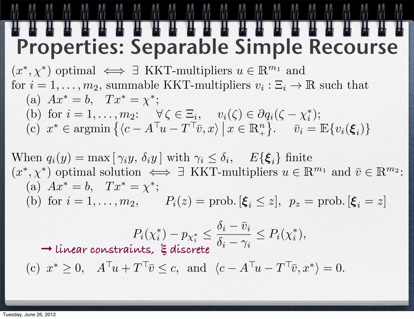
Properties: Separable Simple Recourse
➞ linear constraints, ξ discrete
(x∗,χ∗) optimal ⇐⇒ ∃ KKT-multipliers u ∈ m1 andfor i = 1, . . . ,m2, summable KKT-multipliers vi : Ξi → such that
(a) Ax∗ = b, Tx∗ = χ∗;(b) for i = 1, . . . ,m2: ∀ ζ ∈ Ξi, vi(ζ) ∈ ∂qi(ζ − χ∗
i );(c) x∗ ∈ argmin
��c−A�u− T�v, x�
��x ∈ n+
�. vi = {vi(ξi)}
When qi(y) = max [ γiy, δiy ] with γi ≤ δi, E{ξi} finite(x∗,χ∗) optimal solution ⇐⇒ ∃ KKT-multipliers u ∈ m1 and v ∈ m2 :
(a) Ax∗ = b, Tx∗ = χ∗;(b) for i = 1, . . . ,m2, Pi(z) = prob. [ξi ≤ z], pz = prob. [ξi = z]
Pi(χ∗i )− pχ∗
i≤ δi − vi
δi − γi≤ Pi(χ
∗i ),
(c) x∗ ≥ 0, A�u+ T�v ≤ c, and �c−A�u− T�v, x∗� = 0.
Tuesday, June 26, 2012

Approximation
1
l
l
P
Q
Let P : → [0, 1] continuous, increasing on interval Ξ,
Eψ(χ) = δ(ξ − χ) + (δ − γ)�χP (χ)−
� χ
−∞ζ P (dζ)
�;
Hence,
P (χ∗) =
δ − v
δ − γ=: κ, χ∗
= P−1(κ).
When Q has the same κ-quantile, Q−1(κ) = P−1
(κ), same optimal sol’n.
=⇒ choose Q is ‘quantile close’ to P
Tuesday, June 26, 2012

Lagrangian Dualitymin f0(x), x ∈ X ⊂ n polyhedral
�Ai, x� ≥ bi, i = 1, . . . , s, �Ai, x� = bi, i = s+ 1, . . . ,mThe Lagrangian:
L(x, y) = f0(x) + �y, b−Ax� on X × Y, Y = s+ × m−s.
x∗optimal ⇐⇒ ∃ a pair (x∗, y∗) that satisfies:x∗ ∈ argminx∈ n L(x, y∗), y∗ ∈ argmaxy∈Y L(x∗, y).
primal & dual problems:linear programs: min�c, x�, Ax = b, x ≥ 0 & max�b, y�, A�y ≤ 0quadratic programs: min�c, x�+ 1
2 �x,Qx�, Ax ≥ b, x ∈ n
maxα+ �d, y� − 12 �y, Py�, y ∈ m
+
α = − 12 �c, Q−1c�, d = b+AQ−1c and P = AQ−1A�.
Tuesday, June 26, 2012

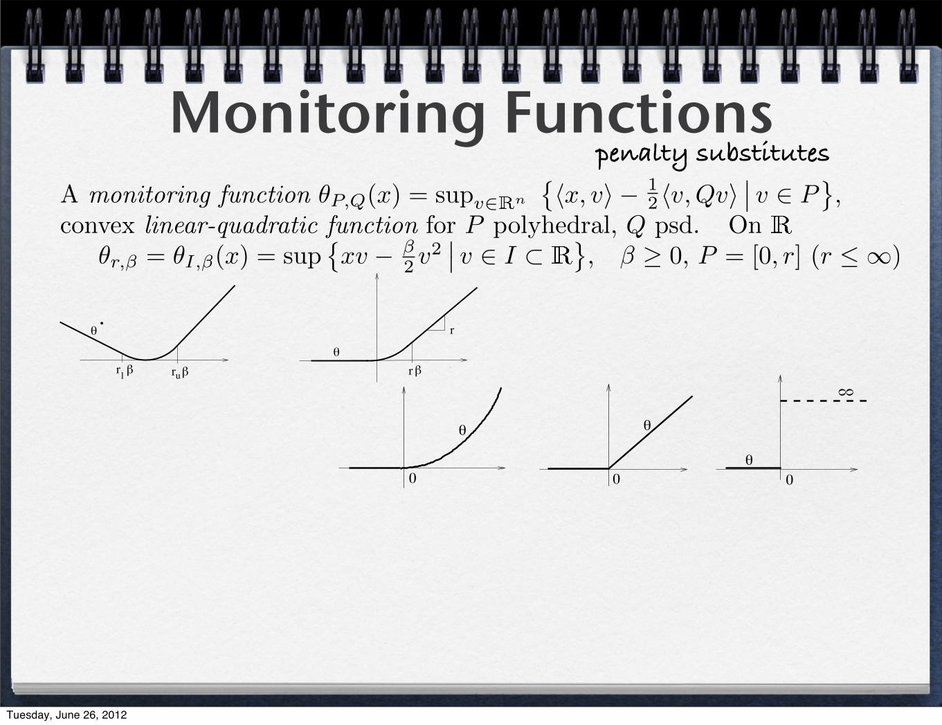
Monitoring Functionspenalty substitutes
A monitoring function θP,Q(x) = supv∈ n
��x, v� − 1
2 �v,Qv��� v ∈ P
�,
convex linear-quadratic function for P polyhedral, Q psd. On
θr,β = θI,β(x) = sup�xv − β
2 v2�� v ∈ I ⊂
�, β ≥ 0, P = [0, r] (r ≤ ∞)
.
Tuesday, June 26, 2012
Monitoring Functionspenalty substitutes
A monitoring function θP,Q(x) = supv∈ n
��x, v� − 1
2 �v,Qv��� v ∈ P
�,
convex linear-quadratic function for P polyhedral, Q psd. On
θr,β = θI,β(x) = sup�xv − β
2 v2�� v ∈ I ⊂
�, β ≥ 0, P = [0, r] (r ≤ ∞)
.r
rr rl u
oo
0 00
Tuesday, June 26, 2012
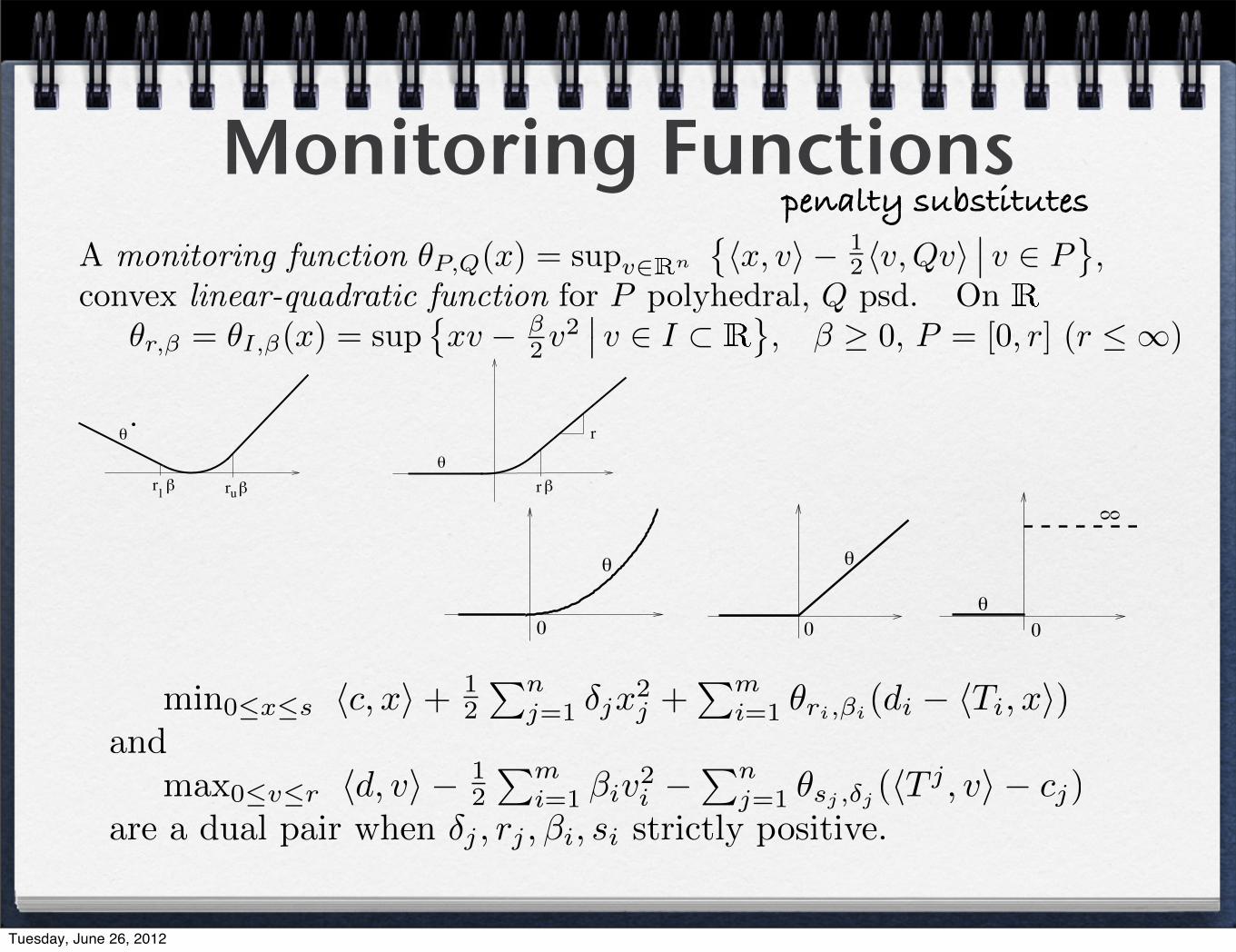
Monitoring Functionspenalty substitutes
A monitoring function θP,Q(x) = supv∈ n
��x, v� − 1
2 �v,Qv��� v ∈ P
�,
convex linear-quadratic function for P polyhedral, Q psd. On
θr,β = θI,β(x) = sup�xv − β
2 v2�� v ∈ I ⊂
�, β ≥ 0, P = [0, r] (r ≤ ∞)
.
min0≤x≤s �c, x�+ 12
�nj=1 δjx
2j +
�mi=1 θri,βi(di − �Ti, x�)
andmax0≤v≤r �d, v� − 1
2
�mi=1 βiv2i −
�nj=1 θsj ,δj (�T j , v� − cj)
are a dual pair when δj , rj ,βi, si strictly positive.
r
rr rl u
oo
0 00
Tuesday, June 26, 2012
Lake Stoöpt
I
II
III
IV
Treatment plant
Reed basin
i
iexcellent acceptable unacceptable
i
i
r
r
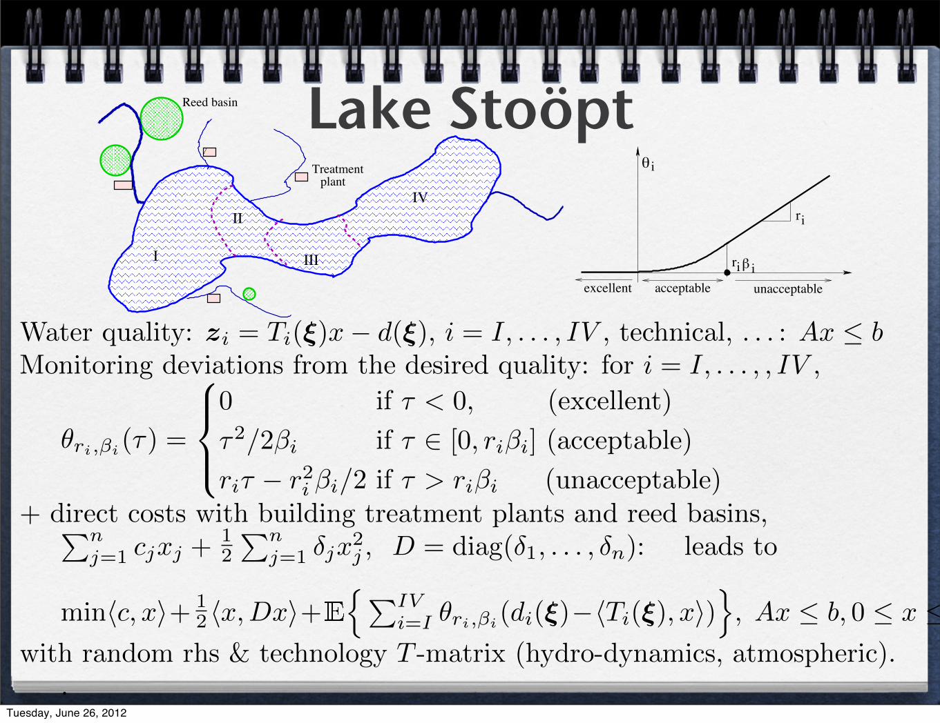
Water quality: zi = Ti(ξ)x− d(ξ), i = I, . . . , IV , technical, . . . : Ax ≤ bMonitoring deviations from the desired quality: for i = I, . . . , , IV ,
θri,βi(τ) =
0 if τ < 0, (excellent)
τ2/2βi if τ ∈ [0, riβi] (acceptable)
riτ − r2i βi/2 if τ > riβi (unacceptable)+ direct costs with building treatment plants and reed basins,�n
j=1 cjxj +12
�nj=1 δjx
2j , D = diag(δ1, . . . , δn): leads to
min�c, x�+ 12 �x,Dx�+
��IVi=I θri,βi(di(ξ)−�Ti(ξ), x�)
�, Ax ≤ b, 0 ≤ x ≤ s
with random rhs & technology T -matrix (hydro-dynamics, atmospheric)..
Tuesday, June 26, 2012

Exploiting dualitymin �c, x�+ 1
2 �x,Dx�+�m2
i=1
i{θri,βi(wi)}, Ax ≥ b, w = d−Tx, 0 ≤ x ≤ s
for all i, ξi = (ri,βi,di, ti1, . . . , tin), w and, later, v as very long vectors.
The dual takes on the form, with u ≥ 0, 0 ≤ vi ≤ ri, ∀ i
max �b, u� −n�
j=1
θsj ,δj (zj) +m2�
i=1
Ei{divi − 12βiv
2i }
such that zj = �Aj , u�+m2�
i=1
Ei{tijvi}− cj , j = 1, . . . , n,
Only “simple” stochastic box constraints: 0 ≤ vi ≤ ri, i = 1, . . . ,m2.Lake Stoopt: r and β are non-random.
.
Tuesday, June 26, 2012

Lagrangian Finite Generation
Step 0. V ν = [v1, . . . ,vν ], vki : Ξi → [0, ri], ∀i
Step 1. Compute dν = E{V �ν d}, Bν = E{V �
ν BV ν}, T�ν = E{T�V ν}
Step 2. Solve the (deterministic) approximating dual program:max �b, u�+ �dν ,λ� − 1
2 �λ, Bνλ� −�n
j=1 θsj ,δj (zj)
s.t A�u+ T�ν λ− z = c,
�νk=1 λk = 1, u ≥ 0, λ ≥ 0
(uν ,λν , zν) optimal, and xν KKT-multipliers of equality constraints.set vν = V νλν , wν
i = di − �T i, xν�, i = 1, . . . ,m2
Step 3 (saddle point check) Stop, if for each i,vνi ∈ argmaxvi∈[0,ri] �w
νi ,vi� − 1
2βiv2i ,
otherwise, for i = 1, . . . ,m2 and every ζ ∈ Ξi, definevν+1i (ζ) ∈ argmax 0≤υ≤ri [w
νi (ζ)υ − 1
2βiυ2] with value θri,βi(wν
i (ζ))Augment V ν+1 = [V vν+1], set ν ← ν + 1, return to Step 1.
r2
r10
v
v
v
v
v
+1
2
1
Tuesday, June 26, 2012