stochastic processes and their applications in computer … · 2006-06-23 · continuous...
TRANSCRIPT

1
Bi04a_1
© Copyright W. Schreiner 2005
StochasticStochastic ProcessesProcesses and and theirtheir ApplicationsApplicationsin Computer in Computer SimulationsSimulations
forfor BioinformaticsBioinformatics
Unit 04a:
Bi04a_2
© Copyright W. Schreiner 2005
StochasticStochastic ProcessesProcesses and and theirtheir ApplicationsApplications in in Computer Computer SimulationsSimulations forfor BioinformaticsBioinformatics
Basic Probability Concepts revisitedCrude Monte CarloMarkov-Chain Monte Carlo
a) Metropolis-Hastingsb) Gibbs-Sampling
Real Example: How to find the Consensus Sequence (Unit 4c, Start)
Simulated Annealing using Markov-Chain-Monte CarloReal Example: How to find the Consensus Sequence (Unit 4c, ctd)
Genetic Algorithmsa) General applications used to optimize structure of multidimensional
objects: molecule conformations, sequence alignments, etc.Real example: Multiple sequence alignment by GA Program SAGA
b) Genetic Computing: Genetic Algorithms used to optimize computerprograms

2
Bi04a_3
© Copyright W. Schreiner 2005
Basic Basic ProbabilityProbability ConceptsConcepts revisitedrevisited
Discrete distributionsabsolute frequenciesrelative frequencieslimiting behaviours as N ∞probabilites & cumulative probabilities
Continuous distributionsabsolute frequenciesrelative frequencieslimiting behaviours as N ∞probabilites & cumulative probabilities
Bi04a_4
© Copyright W. Schreiner 2005
{ }1 2 3 4 5 6
6
1
61 21 2 6
6
1
, , , , , ,
, ,...
1
"
=
=
=
⎧ ⎫= = =⎨ ⎬⎩ ⎭
=
∑
∑
ii
ii
H H H H H H absolute Frequences
H N Summation Condition for absolute Frequences
HH Hh h h relative frequencesN N N
h Normalization Condition for relative Frequences
irgendein Wert muß ..."ja schließlich auftreten
Basic Basic ConceptsConcepts revisitedrevisited
1. Discrete Distributionsrandom variable takes only a few possible values
H3-times dice shows „3“
example: ξ ∈ {1, 2, 3, 4, 5, 6} for (normal) diceN-times throwing a dice:
3
Bi04a_5
© Copyright W. Schreiner 2005
Basic Basic ConceptsConcepts revisitedrevisited
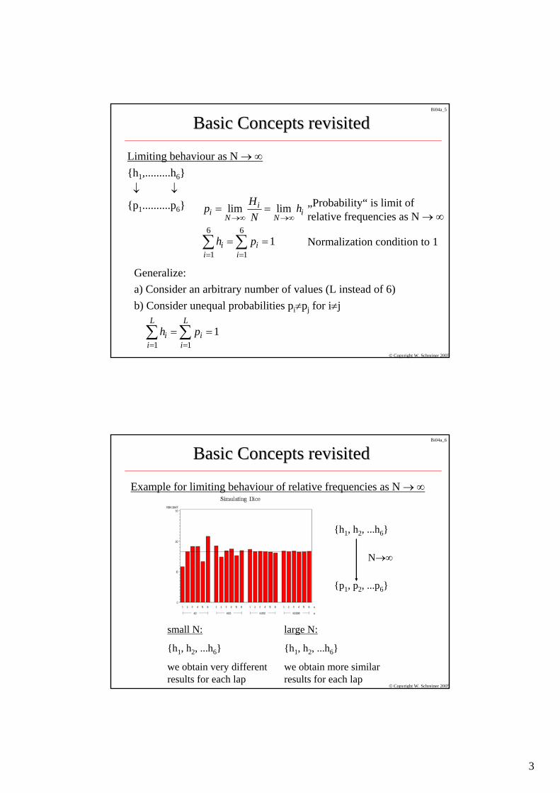
Limiting behaviour as N →∞
Generalize:a) Consider an arbitrary number of values (L instead of 6)b) Consider unequal probabilities pi≠pj for i≠j
{h1,.........h6}↓ ↓
{p1..........p6} „Probability“ is limit of relative frequencies as N →∞
Normalization condition to 16 6
1 1
lim lim
1
→∞ →∞
= =
= =
= =∑ ∑
ii iN N
i ii i
Hp hN
h p
1 11
= == =∑ ∑
L L
i ii i
h p
Bi04a_6
© Copyright W. Schreiner 2005
Basic Basic ConceptsConcepts revisitedrevisited
Example for limiting behaviour of relative frequencies as N →∞
small N:
{h1, h2, ...h6}
we obtain very different results for each lap
large N:
{h1, h2, ...h6}
we obtain more similarresults for each lap
{h1, h2, ...h6}
N→∞
{p1, p2, ...p6}

4
Bi04a_7
© Copyright W. Schreiner 2005
Basic Basic ConceptsConcepts revisitedrevisited
“cumulative probability”
“probability distribution”
p(i) = Pr(ξ=i)
F(i) = Pr(ξ≤i)
( ) ( )1=
=∑i
lF i p i
Bi04a_8
© Copyright W. Schreiner 2005
Basic Basic ConceptsConcepts revisitedrevisited
A simple example:
normal dice
“Mafia” dice
0 1 2 3 4 5 6
1/6
1
p
F
0 1 2 3
p F1
1/6
( )
( ) ( )
1
1
1=
=
=
=
∑
∑
L
li
l
p l
F i p l

5
Bi04a_9
© Copyright W. Schreiner 2005
Basic Basic ConceptsConcepts revisitedrevisited
2. Continuous Distributionsrandom variable takes arbitrary (real) values within given intervallex.: ξ ∈ , 0 ≤ ξ ≤ 1
-2 ≤ ξ ≤ 50 ≤ ξ ≤ ∞
-∞ ≤ ξ ≤ ∞
finite intervals
infinite intervals
Bi04a_10
© Copyright W. Schreiner 2005
p(x) is defined such that
Pr(x ≤ ξ ≤ x + dx) = p(x)dx dx ... infinitesimally small interval
shaded area
[a,b] ... “real” intervall Normalization for probability density function (p.d.f.)“irgendwo muß ξ ja liegen”
( ) ( )Pr 1∞
−∞
−∞ ≤ ≤ ∞ = =∫ p dξ ξ ξ( ) ( )Pr ≤ ≤ = ∫b
a
a b p dξ ξ ξ
Basic Basic ConceptsConcepts revisitedrevisitedContinuous Distributions, ctd.
Since the random variable can take any (in between) value, the concept of
discrete probability values
must be generalized to a
continuous probability distribution function
uniform distributionp(x)1
x x+dx1
ξ

6
Bi04a_11
© Copyright W. Schreiner 2005
Basic Basic ConceptsConcepts revisitedrevisited
Continuous Distributions, ctd.specifically consider interval [-∞,x]
P(-∞ ≤ ξ ≤ x ) =
probabilitydensityfunction(p.d.f.)
cumulativedistribution
function
if this holds, we know from calculus:
F(-∞) = 0F(+∞) = 1F(x) is increasing since p(x)≥0
F(x)p
x 1ξ
1p(x)
( ) ( ) ( )Pr= = ≤∫x
p d F x xξ ξ ξ
( ) ( )=dp x F xdx
Bi04a_12
© Copyright W. Schreiner 2005
( )
( )
11 2
0 0
2 2
00
2 1 0 12
= = − =
= =
∫
∫x
x
xp x dx
p d xξ ξ ξ
Basic Basic ConceptsConcepts revisitedrevisited
Example: linearly increasing p.d.f. on [0,1]:p(x) = 2x
Normalization:
Cumulativedistribution function:p(x)
F(x)
7
Bi04a_13
© Copyright W. Schreiner 2005
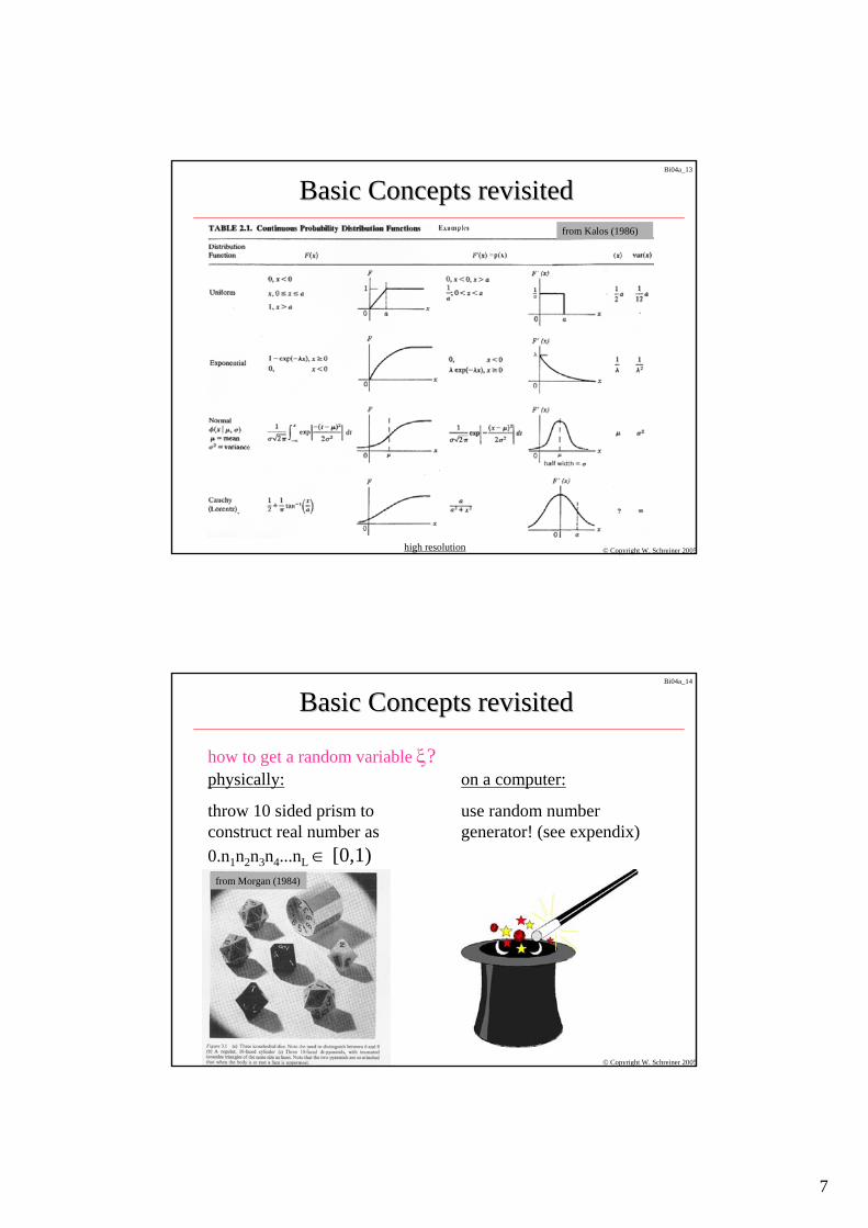
Basic Basic ConceptsConcepts revisitedrevisited
high resolution
from Kalos (1986)
Bi04a_14
© Copyright W. Schreiner 2005
Basic Basic ConceptsConcepts revisitedrevisited
how to get a random variable ξ?physically:
throw 10 sided prism to construct real number as 0.n1n2n3n4...nL ∈ [0,1)
on a computer:
use random numbergenerator! (see expendix)
from Morgan (1984)

8
Bi04a_15
© Copyright W. Schreiner 2005
ExpendixExpendix 1: 1: HowHow to to generategenerate randomrandom numbersnumbers
„Real“ random numbers (fromnature, i.e. physical process)
„Pseudo“ random numbers (PRNs) (from computer programs)
xn+1=a•xn+b (mod m)„congruential method“e.g. a = 1573, b = 19, m = 1000, x0 =89
seed
from Morgan (1984)
[0,1]= ∈nn
x uniform distributedm
ξ
Bi04a_16
© Copyright W. Schreiner 2005
ReallyReally randomrandom versus versus PseudoPseudo randomrandom..
„Real“ random numbers (fromnature, i.e. physical process)
„Pseudo“ random numbers (PRNs) (from computer programs)
no prediction possiblerandomness (of e.g. dice) due to uncertaincy principle of quantum physics
strictly predictable“randomness” due to algorithm, its parameters & seed
statistical tests will not reveal systematic predictabilityawkward for simulation
statistical tests will not easily reveal systematic predictabilityhowever: beware of loopshandy for simulation

9
Bi04a_17
© Copyright W. Schreiner 2005
ExpendixExpendix 1: 1: PRNsPRNs QualityQuality
„Bad Generator“ „Improved Generator“
high resolution high resolution
from Morgan (1984)
Bi04a_18
© Copyright W. Schreiner 2005
ExpendixExpendix 1: 1: PRNsPRNs fromfrom mostmost commoncommondistributionsdistributions
ξ ∈ [0,1] uniformly distributed is available in (almost) every programinglanguage (library)
ξ ∈ N(µ,σ) normal (Gaussian) distribution
is available in many programing language (libraries)mean standard deviation
high resolution
high resolutionfrom Kalos (1986)
from Kalos (1986)

10
Bi04a_19
© Copyright W. Schreiner 2005
ExpendixExpendix 1:1:Ho to Ho to getget PRNsPRNs fromfrom otherother distributionsdistributions
statistical and mathematical program librariesderiving desired distribution from uniform PRNs on [0,1]:
inversion methodother, even more sophisticated methods ...rejection method (works for arbitrary distributions wanted!)table lookup-method
Bi04a_20
© Copyright W. Schreiner 2005
ExpendixExpendix 1: Linear 1: Linear transformationstransformations of of PRNsPRNsuniform PRNs → uniform PRNsGaussian PRNs → Gaussian PRNsarbitrary distributed PRNs → (? not generally predictable)
ξ →N. ξ ∈[0,N]
ξ →2 ξ-1 ∈[-1,+1]
ξ →A+(B-A) ξ ∈[A,B]
CAUTION:what happens at start & end of interval!
!
10
0 N
trafo
A B-
0 1
trafo
-1
1
+1
0
0
trafo

11
Bi04a_21
© Copyright W. Schreiner 2005
( ) ( ) ( ) ( )
( ) ( )
( ) ( )
( )1
Pr
−
= ≤ = ≤ =
= ⋅
= ⋅
⎛ ⎞= ⎜ ⎟⎝ ⎠
y x
xy
y x
dF y Y y X x F Xdy
d F x dxf ydx dy
dxf y f xdy
dyf xdx
ExpendixExpendix 1: General 1: General transformationstransformations of of PRNsPRNs
considercumulativedistribution
functionfor
argumentation
And for details: see Morgan (1984), p.29 or Kalos (1986), p.40
taking absolute values | | will make formulavalid for decreasing and increasingtransformation functions!
high resolution
from Morgan (1984)
Apply differentiatiation operator to both sides of equation!
Use chain-rule for differentiation
Bi04a_22
© Copyright W. Schreiner 2005
ExpendixExpendix 1: General 1: General transformationstransformations of of PRNsPRNs
An illustration of thetransformationy = √x
relating the densities
fX(x) = e-x, fY (y) = 2ye-y2.
The shaded regions haveequal areas.
high resolution
from Morgan (1984)
12
Bi04a_23
© Copyright W. Schreiner 2005
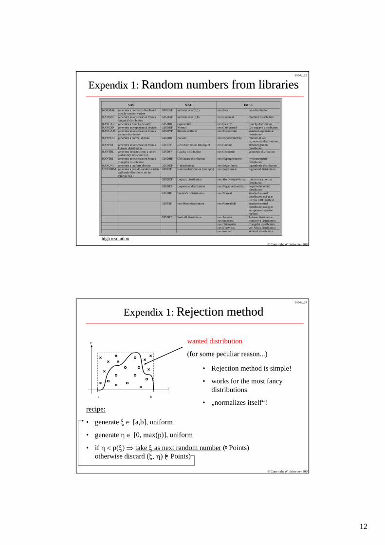
ExpendixExpendix 1: 1: RandomRandom numbersnumbers fromfrom librarieslibraries
high resolution
SAS NAG IMSLNORMAL generates a normally distributed
pseudo-random variateG05CAF uniform over (0,1) nextBeta beta distribution
RANBIN generates an observation from abinomial distribution
G05DAF uniform over (a,b) nextBinomial binomial distribution
RANCAU generates a Cauchy deviate G05DBF exponential nextCauchy Cauchy distributionRANEXP generates an exponential deviate G05DDF Normal nextChiSquared Chi-squared distributionRANGAM generates an observation from a
gamma distributionG05DYF discrete uniform nextExponential standard exponential
distributionRANNOR generates a normal deviate G05DRF Poisson nextExponentialMix mixture of two
exponential distributionsRANPOI generates an observation from a
Poisson distributionG05FEF Beta distribution (multiple) nextGamma standard gamma
distributionRANTBL generates deviates from a tabled
probability mass functionG05DFF Cauchy distribution nextGeometric geometric distribution
RANTRI generates an observation from atriangular distribution
G05DHF Chi-square distribution nextHypergeometric hypergeometricdistribution
RANUNI generates a uniform deviate G05DKF F-distribution nextLogarithmic logarithmic distributionUNIFORM generates a pseudo-random variate
uniformly distributed on theinterval (0,1)
G05FFF Gamma distribution (multiple) nextLogNormal lognormal distribution
G05DCF Logistic distribution nextMultivariateNormal multivariate normaldistribution
G05DEF Lognormal distribution nextNegativeBinomial negative binomialdistribution
G05DJF Student's t-distribution nextNormal standard normaldistribution using aninverse CDF method
G05FSF von Mises distribution nextNormalAR standard normaldistribution using anacceptance/rejectionmethod
G05DPF Weibull distribution nextPoisson Poisson distributionnextStudentsT Student's t distributionnext Triangular triangular distributionnextVonMises von Mises distributionnextWeibull Weibull distribution
Bi04a_24
© Copyright W. Schreiner 2005
ExpendixExpendix 1: 1: RejectionRejection methodmethod
wanted distribution
(for some peculiar reason...)
a
ξ
p
b
• Rejection method is simple!
• works for the most fancydistributions
• „normalizes itself“!recipe:
• generate ξ ∈ [a,b], uniform
• generate η ∈ [0, max(p)], uniform
• if η < p(ξ) ⇒ take ξ as next random number ( Points)otherwise discard (ξ, η) ( Points)

13
Bi04a_25
© Copyright W. Schreiner 2005
ExpendixExpendix 1: 1: RejectionRejection methodmethod, , ctdctd..rejection method is simple but:
may be inefficient: „Simple but dead slow!“
Bi04a_26
© Copyright W. Schreiner 2005
ExpendixExpendix 1: 1: SelectSelect randomlyrandomly fromfrom a a groupgroup of n of n individualsindividuals accordingaccording to to weightsweights ((probabilitiesprobabilities))
(„table lookup method for a discrete random variable“)
1) Case 1: equal probabilities (=weights)
equidistant intervals
individual #
ξ
0 1/n 2/n 3/n . . . . . . . . . . . . . . .(n-1)/n n/n = 1
1 2 3 n
recipe:
• draw pseudo random number ξ from uniform distribution over [0,1]
• individual selected: ( )int 1, min ,1/⎡ ⎤= + =⎢ ⎥⎣ ⎦
i i i nnξ

14
Bi04a_27
© Copyright W. Schreiner 2005
( ) ( )1
/ /
1 1: 1
−− −
= =
⎡ ⎤= =⎢ ⎥⎢ ⎥⎣ ⎦∑ ∑i in n
E s E si i
i ip e e Normalization pτ τ
ExpendixExpendix 1: 1: SelectSelect randomlyrandomly fromfrom a a groupgroup of n of n individualsindividuals accordingaccording to to weightsweights ((probabilitiesprobabilities))
2) Case 2: different probabilities (=weights), e.g. pi proportional e-E(si)/τ
recipe:
• draw pseudo random number ξ from uniform distribution over [0,1]
• individual i selected so that:
ξ
equidistant intervals
individual # 1 2 3 4 5 6 7 . . . n
0 1
(„table lookup method for a discrete random variable“)
1
1 1
−
= =
< ≤∑ ∑i i
l ll l
p pξ
Bi04a_28
© Copyright W. Schreiner 2005
LiteratureLiterature on on RandomRandom NumbersNumbers
Morgan,B.J.T. 1984. Elements of Simulation. Chapman and Hall, New York.
Rosanow,J.A. 1974. Wahrscheinlichkeitstheorie. Rowohlt Taschenbuch Verlag, Hamburg.
Kalos,M.H. and P.A.Whitlock 1986. Monte Carlo methods. Wiley, New York.
SAS Institute. 1985. SAS User's Guide: Basics. Cary.
NAg. 1993. Fortran Library Mark 16. Oxford.
JMSL Reference Manual. 2002. Visual Numerics, San Ramon. http://www.vni.com/books/docs/