Stochastic Programming in Transportation

and Logistics

Warren B. Powell and Huseyin Topaloglu

Department of Operations Research and Financial Engineering, PrincetonUniversity, Princeton, NJ 08544

Abstract

Freight transportation is characterized by highly dynamic information processes:customers call in orders over time to move freight; the movement of freight overlong distances is subject to random delays; equipment failures require last minutechanges; and decisions are not always executed in the field according to plan. Thehigh-dimensionality of the decisions involved has made transportation a naturalapplication for the techniques of mathematical programming, but the challenge ofmodeling dynamic information processes has limited their success. In this chapter,we explore the use of concepts from stochastic programming in the context of re-source allocation problems that arise in freight transportation. Since transportationproblems are often quite large, we focus on the degree to which some techniquesexploit the natural structure of these problems. Experimental work in the contextof these applications is quite limited, so we highlight the techniques that appear tobe the most promising.

Preprint submitted to Elsevier Preprint 8 January 2003

Contents

1 Introduction 1

2 Applications and issues 2

2.1 Some sample problems 2

2.2 Sources of uncertainty 5

2.3 Special modeling issues in transportation 7

2.4 Why do we need stochastic programming? 8

3 Modeling framework 9

3.1 Resources 10

3.2 Processes 12

3.3 Controls 16

3.4 Modeling state variables 17

3.5 The optimization problem 18

3.6 A brief taxonomy of problems 19

4 A case study: freight car distribution 22

5 The two-stage resource allocation problem 25

5.1 Notational style 26

5.2 Modeling the car distribution problem 28

5.3 Engineering practice - Myopic and deterministic models 30

5.4 No substitution - a simple recourse model 33

5.5 Shipping to regional depots - a separable recourse model 35

5.6 Shipping to classification yards - a network recourse model 45

5.7 Extension to large attribute spaces 55

i

6 Multistage resource allocation problems 56

6.1 Formulation 57

6.2 Our algorithmic strategy 59

6.3 Single commodity problems 65

6.4 Multicommodity problems 66

6.5 The problem of travel times 69

7 Some experimental results 71

7.1 Experimental results for two-stage problems 72

7.2 Experimental results for multistage problems 73

8 A list of extensions 77

9 Implementing stochastic programming models in the real world 78

10 Bibliographic notes 80

ii

1 Introduction

Operational models of problems in transportation and logistics offer a ripe set of applica-tions for stochastic programming since they are typically characterized by highly dynamicinformation processes. In freight transportation, it is the norm to call a carrier the daybefore, or sometimes the same day, to request that a shipment be moved. In truckloadtrucking, last minute phone calls are combined with requests that can be made a few daysin advance, putting carriers in the position of committing to move loads without knowingthe last minute demands that will be made of them (sometimes by their most importantcustomers). In railroads, requests to move freight might be made a week in the future, butit can take a week to move a freight car to a customer. The effect is the same.

The goal of this chapter is to provide some examples of problems, drawn from the arenaof freight transportation, that appear to provide a natural application of stochastic pro-gramming. Optimization models in transportation and logistics, as they are applied inpractice, are almost always formulated based on deterministic models. Our intent is toshow where deterministic models can exhibit fundamental weaknesses, not from the per-spective of academic theory, but in terms of practical limitations as perceived by peoplein industry. At the same time, we want to use the richness of real problems to raise issuesthat may not have been addressed by the stochastic programming community. We wantto highlight what works, what does not, and where there are rich areas for new research.

We do not make any effort to provide a comprehensive treatment of stochastic optimiza-tion problems in transportation and logistics. First, we consider only problems in freighttransportation (for the uninitiated, “transportation and logistics” refers to the operationalproblems surrounding the movement of goods). These problems are inherently discrete,giving rise to stochastic, integer programming problems, but we focus on problems wherelinear programming formulations represent a good starting point. We completely avoid thegeneral area of stochastic vehicle routing or the types of batch processes that often arisein the movement of smaller shipments, and focus instead on problems that can be broadlydescribed as dynamic resource allocation problems.

Our presentation begins in section 2 with an overview of different classes of applications.This section provides a summary of the different types of uncertainty that arise, and ad-dresses the fundamental question of why stochastic programming is a promising technologyfor freight transportation. Section 3 provides a general modeling framework that representsa bridge between linear programming formulations and a representation that more explic-itly captures the dimensions of transportation applications. In section 4 we present a casestudy based on the distribution of freight cars for a railroad. This case study provides uswith a problem context where dynamic information processes play an important role. We

1

use this case study in the remainder of the chapter to keep our discussions grounded inthe context of a real application.

We approach the stochastic modeling of our freight car problem in two steps. First, wediscuss in section 5 the basic two-stage resource allocation problem. This problem is partic-ularly relevant to the car distribution problem. The characteristics of the car distributionproblem nicely illustrate different types of recourse strategies that can arise in practice.Specialized strategies give way to approximations which exploit the underlying networkstructure. For the most general case (network recourse) we briefly review a broad rangeof stochastic programming strategies, focusing on their ability to handle the stucture oftransportation problems.

Section 6 addresses multistage problems. Our approach toward multistage problems is thatthey can and should be solved as sequences of two-stage problems. As a result, we solvemultistage problems by building on the theory of two-stage problems.

Transportation problems offer far more richness than can be covered in a single chapter.Section 8 provides a hint of the topics that we do not attempt to cover. We close withsection 9 that discusses some of the challenges of actually implementing stochastic modelsin an operational setting.

2 Applications and issues

It is important to have in mind a set of real problems that arise in transportation andlogistics. We begin our discussion of applications by listing some sample problems thatarise in practice, and then use these problems a) to discuss sources of uncertainty, b) toraise special modeling problems that arise in transportation applications, and finally c) tohighlight, from a practical perspective, the limitations of deterministic models and howstochastic programming can improve the quality of our models from a practical perspective.

2.1 Some sample problems

Transportation, fundamentally, is the business of moving things so that they are moreuseful. If there is a resource at a location i, it may be more useful at another location j.Within this simple framework, there is a tremendous variety of problems that pose specialmodeling and algorithmic issues. Below is a short list of problems that helps to highlightsome of the modeling issues that we will have to grapple with.

2

1) Product distribution - Perhaps one of the oldest and most practical problems is thedetermination of how much product to ship from a plant to intermediate warehousesbefore finally shipping to the retailer (or customer). The decision of how much and whereto ship and where must be made before we know the customer demand. There are anumber of important variations of this problem, including:

a) Separability of the distribution process - It is often the case that each customer willbe served by a unique warehouse, but substitution among warehouses may be allowed.

b) Multiple product types with substitution - A company may make multiple producttypes (for example, different types of salty food snacks) for a market that is willingto purchase different products when one is sold out. For the basic single period dis-tribution problem, substitution between products at different locations is the same assubstitution across different types of products, as long as the substitution cost is known(when the cost is a transportation cost, this is known, whereas when it represents thecost of substituting for different product types, it is usually unknown).

c) Demand backlogging - In multiperiod problems, if demand is not satisfied in one timeperiod, we may assume the demand is lost or backlogged to the next time period. Wemight add that the same issue arises in the product being managed; highly perishableproducts vanish if not used at a point in time, whereas nonperishable products stayaround.

2) Container management - Often referred to as fleet management in the literature, “con-tainers” represent boxes of various forms that hold freight. These might be trailers,boxcars, or the intermodal containers that are used to move goods across the oceans(and then by truck and rail to inland customers). Containers represent a reusable re-source where the act of satisfying a customer demand (moving freight from i to j) alsohas the effect of changing the state of the system (the container is moved from i and j).The customer demand vanishes from the system, but the container does not. Importantproblem variations include:

a) Single commodity problems - These arise when all the containers are the same, orwhen there are different container types with no substitution between different typesof demands. When there is no substitution, the problem decomposes into a series ofsingle commodity problems for each product type.

b) Multicommodity problems - There may be different container types, and the customersmay be willing to substitute between them. For example, they may accept a biggercontainer, or be willing to move their dry goods in a refrigerated trailer (although norefrigeration is necessary).

c) Time windows and demand backlogging - The most common model represents cus-tomer demands at a point in time, where they are lost if they are not served at thatpoint in time. In practice, it is usually the case that customer orders can be delayed.

d) Transshipment and relay points - The simplest models represent a demand as the needto move from i to j, and where the movement is represented as a single decision. More

3

complex operations have to model transportation legs (ocean or rail movements) withrelays or transshipment points (ports, rail yards) where the containers move from onemode to the next. A major element of complexity is when capacity constraints areimposed on the transportation legs.

3) Managing complex equipment - The major railroads in North America need to managefleets of several thousand locomotives. The air mobility command has to move freightand people on a global scale using different types of aircraft. Recently formed companiesservice a high end market with personal jet service using jets in which the customers owna fraction. These problems have been modeled in the past using the same framework ascontainer management problems with multiple container types. These complex pieces ofequipment require something more. For example, there are four major classes of locomo-tive, reflecting whether they are high or low “adhesion” (a technology that determinesthe slippage of the wheels on a rail), and whether they are four axle or six axle units (sixaxle locomotives are more powerful). On closer inspection, we find that the horsepowerrating of a locomotive can be divided into 10 or 12 reasonable divisions. It matters ifthe locomotive has its home shop in Chicago, Atlanta or southern California. Since lo-comotives may move from the tracks of one railroad to another, it matters who owns thelocomotive. And it matters if the locomotive is due into the shop in 1, 2, . . . , 10 days,or more than 10 days. In short, complex equipment is complex, and does not lend itselfeasily to a multicommodity formulation. As we show later, this characteristic determineswhether the size of the attribute space of a resource is small enough to enumerate theentire space, or too large to enumerate.

4) People and crews - Trucks, trains and planes move because people operate them. Notsurprisingly, the modeling of the people is not only important, but requires a set ofattributes that makes complex equipment look simple. A truck driver, for example,might be characterized by his current location, his home base, his skill level, whether hehas experience driving into Mexico or Canada, how many hours he has driven in the lasteight days, how many consecutive hours he has been “on duty” today, and how manyhours he has been actively driving during his current duty period. Production systemshave to cover these and many other issues.

These problems are all examples of resource allocation problems where, with few excep-tions, a single “resource” serves a single “demand.” “Bundling” arises when, for example,you need several locomotives to pull a single train, or two drivers (a sleeper team) tooperate a single truck. “Layering” arises when you need an aircraft, a pilot, fuel and spe-cial loading equipment to move a load from one airbase to another. In some cases, theresource/task dichotomy breaks down. For example, we may be managing locomotives,crews and boxcars. The boxcar needs to go from A to B. We need the crew to move thetrain, but the crew needs to get back to its home domicile at C. And the locomotive needs

4

to get to shop at D. We would refer to the locomotives, crew and boxcars as three resourcelayers, since the locomotives, crew and boxcars are all needed to move the train. In fact,for more complex problems, we refer to the objects being managed as resource layers (orsometimes, resource classes), where one layer is almost always one that would be referredto as a customer, or job, or task.

2.2 Sources of uncertainty

Uncertainty arises whenever we need to make a decision based on information that is notfully known. We are aware of three scenarios under which this can arise:

1) The information is not yet known, but will become known at some point in the future.This is the standard model of uncertainty.

2) Information is known to someone (or something), but is not known to the decision-maker. We would generally say that this information is knowable but for various reasons(most commonly, it is simply too expensive) has not been properly communicated towhere the information is needed for a decision.

3) The information will never be known (optimization under incomplete information). Forany of a variety of economic or technical reasons, an unknown variable is never measured,even though it would help improve decisions. Since the information is never known, weare not able to develop a probability distribution for it.

Cases (2) and (3) above both represent instances where decisions have to be made withoutinformation, but we assume that case (3) represents information that never becomes knownexplicitly, whereas (2) represents the case where someone knows the information, raisingthe possibility that the information could be shared (at a cost) or at a minimum, where aprobability distribution might be constructed after the fact and shared with others.

Classical uncertainty arises because information arrives over time. It is possible to di-vide the different types of dynamic information processes into three basic classes: the “re-sources” being managed (including customer demands), the physical processes that governthe evolution of the system over time, and the decisions that are actually implemented todrive the system. This division reflects our modeling framework, presented in section 3.Since the focus of this volume is on modeling uncertainty, it is useful to give each of theseat least a brief discussion.

Resources:Under the heading of “resources” we include all the information classes that we are activelymanaging. More formally, these are “endogenously controllable information classes whichconstrain the system,” a definition that includes not just the trucks, trains and planes that

5

we normally think of as resources, but also the customer orders that these resources arenormally serving). Dynamic information processes for resources may include:

a) Information about new (exogenous) arrivals to the system - This normally includes thearrival of customer orders, but may also include the arrivals of the product, equipmentor people required to satisfy the customer order. For example, a trucking company isconstantly hiring new drivers (there is a lot of turnover) so the arrival of new drivers tothe fleet is a dynamic information process. Similarly, a railroad has to manage boxcars,and the process of boxcars becoming empty turns out to be a highly stochastic process(far more uncertain than the customer orders).

b) Information about resources leaving the system - Drivers may quit, locomotives maybe retired from service, product can perish. The challenge of modeling departures isthat they depend on the state of the system, whereas exogenous arrivals are normallymodeled as being independent of the state of the system.

c) Information about the state of a resource - An aircraft may break down or a driver maycall in sick.

An important dimension of the modeling of resources is the concept of knowability andactionability. It is not uncommon for a customer to call in and book an order in advance.Thus, the order becomes known right now (time t) but actionable when it actually arrivesto the system at some point in the future (at time t′ ≥ t). Most stochastic models implicitlyassume that a customer demand is not known until it actually arrives. By contrast, mostdeterministic models assume that we know all orders in advance (or more precisely, that wedo not want to make a decision taking into account any order that is not already known).In practice, both extremes arise, as well as the case of prebooking where customers call atleast some of their orders in advance.

Processes:Under this category, we include information about parameters that govern the evolutionof the system over time. The most important classes include:

a) The time required to complete a decision - In most areas of transportation, travel timesare random, and sometimes highly so (although applications vary in the degree to whichrandom arrival times actually matter). In air traffic control problems, planes may landat two minute intervals. Flights of several hours can easily vary in duration by 10 or20 minutes, so they have to maintain a short backlog of flights to ensure that there isalways an aircraft available to land when the runway has the capacity to handle anotherarrival. In railroads, it is not unusual for the travel time between two points to takeanywhere from five to eight days.

b) The cost of a decision - This is often the least uncertain parameter, but there are anumber of reasons why we might not know the cost of a decision until after the fact. Costs

6

which are typically not fully known in advance include tolls, transportation accidents,and processing costs that are not always easy to allocate to a particular activity. Evenmore uncertain is the revenue that might be received from satisfying a customer whichmight arise as a result of complex accounting procedures.

c) Parameters that determine the attributes of a resource after a decision - Examplesmight include the fuel consumption of an aircraft or locomotive (which determines thefuel level), or the maintenance status of the equipment at the end of a trip.

Controls:In real problems, there is a difference between the decisions that we are planning to make,and the decisions that are actually made. The flow of actual decisions is an importantexogenous information process. There are several reasons why an actual physical systemdoes not evolve as planned:

1) The decisions made by a model are not as detailed as what is actually needed in opera-tions. The user has to take a plan developed by the model and convert it into somethingimplementable.

2) The user has information not available to the model.3) The user simply prefers to use a different problem solving approach (possibly suboptimal,

but this assumes the solution provided by the model is in some way optimal).

When there is a difference between what a model recommends and the decisions that areactually made, we encounter an instance of the user noncompliance problem. This is asource of uncertainty that is often overlooked.

2.3 Special modeling issues in transportation

Transportation problems introduce an array of issues that provide special modeling andalgorithmic challenges. These include:

a) Time staging of information - In freight transportation, information arrives over time.This is the heart of any stochastic model.

b) The lagging of information - Often, a customer will call at time t to place an order to beserved at time t′ > t. The same lagging of information may apply to the vehicles used toserve customers. Since we have information about the future, it is tempting to assumethat we can make plans about the future, even before new information becomes known.

c) Complex resource attributes - It is often assumed that the number of different types ofresources is “not too large.” The number of resource types determines the number ofconstraints. In practice, the attributes of resources can be surprisingly complex, creatingproblems where the number of constraints can number in the millions. This is a challenge

7

even for deterministic models, but poses special difficulties in the context of stochasticproblems.

d) Integrality - Many transportation problems exhibit network structure that makes itmuch easier to obtain integer or near-integer solutions. This structure can be easilydestroyed when uncertainty is introduced.

e) Travel times - The common behavior in transportation problems that it takes time tomove from one location to the next is generally a minor issue in deterministic models.In stochastic models, it can introduce major complications. If the travel times are deter-ministic, the result can be a dramatic growth in the size of the state space. However, itis often the case that travel times not only are stochastic, they are not even measurablewhen the trip is initiated.

f) Multi-agent control - Large transportation systems might be controlled by differentagents who control specific dimensions of the system. The decisions of other agents canappear as random variables to a particular agent.

g) Implementation - What we plan may not be the same as what actually happens. Anoverlooked source of uncertainty is the difference between planned and executed deci-sions.

2.4 Why do we need stochastic programming?

There are two types of modeling technologies that are widely used in practice: simulationmodels, which are used almost entirely for planning purposes where there is a need tounderstand the behavior of a system that evolves over time, and deterministic optimizationmodels and algorithms, when there is a need for the computer to recommend what actionshould be taken. Stochastic programming brings the modeling of uncertainty explicitlyinto the process of making a decision (using an optimization algorithm). But, there isa large community of both academic researchers and consultants who feel that they arebeing quite productive with the algorithms that they are developing based on deterministicmodels.

There is a broad perception, in both the academic research community and in engineeringpractice, that deterministic optimization algorithms are “good enough.” In part this canbe attributed to both the mathematical maturity that has been required to understandstochastic models, and the lack of practical, problem-solving tools. But equally important,we need to understand the ways in which stochastic models can provide solutions thatare not just better, but noticeably better in a way that would attract the attention ofindustry. An understanding of these issues will also indicate where stochastic models arenot necessarily appropriate. A partial list of motivations for stochastic models shouldinclude:

8

1) The newsvendor effect - Providing the right amount of resource to meet demand giventhe uncertainty in demand and the relative costs of providing too much or too little. Adeterministic model will never allocate more than the point forecast, even when thereare excess resources. Stochastic models can overallocate or underallocate depending onthe overall availability of resources to meet forecasted demands.

2) Robust allocation - We might need the container in city A or city C, but we are notsure, so we send the truck halfway in between to city B where it can wait and respondto the demand at the last minute. A deterministic model will never send capacity to alocation that does not need it.

3) The value of advance information - Stochastic models can explicit model the stagingof information over time. A carrier might want to know the value of having customersbook orders farther in advance. A proper analysis of this question needs to consider thevalue of reducing the uncertainty in a forecast.

4) Forecasts of discrete items - Sometimes it is necessary to forecast low volume demands;for example, orders might be 1 with probability 0.20 and 0 with probability 0.80. Apoint forecast would produce a demand of 0.20, but a routing and scheduling model isunable to assign 0.20 trucks to the order (the algorithm routes a single truck). Integerrounding amounts to little more than Monte Carlo sampling (simple rounding producesbiases - it is necessary to round based on a random sample whose expectation is thesame).

5) The algorithmic challenge of solving problems over extended planning horizons - Clas-sical optimization algorithms struggle with optimization problems defined over longhorizons, typically as a result of degeneracy. Formulations based on a stochastic “view”of the world produces time-staged problems that are much easier to solve. Sequences oftwo-stage problems are much easier to solve than a single, large integer program.

6) Overoptimizing problems with imperfect data - A deterministic view of the world canproduce problems that are larger and more complex than necessary. An appreciation ofuncertainty, not only of the future but also of the “here and now” data (which in practiceis a major form of uncertainty) produces models that are smaller and more compact.

3 Modeling framework

The first chapter of this handbook provides a basic mathematical framework for multi-stage stochastic programming problems. The problem with these abstract formulations isspanning the gap between generic mathematical formulations and real problems. In thissection, we offer a notational framework that helps to bridge the gap between real-worlddynamic resource allocation problems, and the basic framework of math programming ingeneral, and stochastic programming in particular.

9

We divide our modeling framework between three fundamental dimensions: the resourcesbeing managed, the processes that govern the dynamics of the system, and the structureand organization of controls which manage the system. Our presentation is not the mostgeneral, but allows us to focus on the dimensions that are important for modeling theorganization and flow of information.

3.1 Resources

To help formalize the discussion, we offer the following definition:

Definition 1 A resource is an endogenously controllable information class that constrainsthe system.

From a math programming perspective, a resource is anything that shows up as a righthand side of a constraint (no surprise that these are often referred to as “resource con-straints”). For transportation, resources include trucks, trains, planes, boxcars, containers,drivers/crews, and special equipment that may be needed to complete a trip. Sometimes,but not always, the “demands” being served also meet this definition. For example, theload of freight that we are moving from one location to the next is both endogenouslycontrollable (we often have to determine when to move the load, and sometimes how it isrouted) and it constrains the system.

We describe resources using the following:

CR = The set of resource classes (e.g. tractors, trailers, drivers, freight).Rc = The set of (discrete) resources in class c ∈ CR.ar = The attributes of resource r ∈ Rc, c ∈ CR.Ac = The space of attributes for resource class c ∈ CR, with element ac ∈ Ac. We often use

A to represent the attribute space of a generic resource.

The attribute vector is a very flexible device for describing the characteristics of a resource.In truckload trucking, it might be the case that all trucks are the same, in which case theattribute vector consists only of the location of the truck. In rail car distribution, theattribute vector can be the type of car as well as the location. If the resource is a humanoperator, the vector can grow to include attributes such as the home domicile, days awayfrom home, hours of service, and skill sets.

The definition of the attribute space requires an understanding of how a resource evolvesover time, and in particular the flow of information. For example, an air cargo carrierworking for the military airlift command might have to move a load of cargo from the

10

eastern United States to southeast Asia. This trip might require midair refueling, as wellas stops at several intermediate airbases. Is it necessary to represent the aircraft at each ofthese intermediate points, or is it enough to assign the aircraft to move a load, and thenmodel its status at the destination? The answer depends on the evolution of informationand decisions. For example, if we can completely model all the steps of a trip using theinformation available when the aircraft first takes off from the origin, then there is noneed to model the intermediate points. But we might wish to model the possibility of afailure in the midair refueling, or the failure of the aircraft itself at any of the intermediateairbases. Both of these represent examples of new information arriving to the system,which requires modeling the status of the aircraft just before the new information arrives.The new information may produce new decisions (we may wish to reroute the aircraft) ora change in the dynamics (the aircraft may be unexpectedly delayed at an airbase).

The need to model our aircraft at intermediate points raises a new and even more complexissue. An aircraft that is fully loaded with freight takes on the characteristics of a layered(or composite) resource. That is, we have not only the characteristics of the aircraft, butalso the characteristics of the freight on the aircraft. This sort of layering arises frequentlyin transportation operations. Another example arises in the management of locomotives.A locomotive may be sitting idle at a rail yard, or it may be attached to an inbound train(which is making an intermediate stop). If the locomotive is attached to an inbound train,then we have not only the attributes of the locomotive, but also of the train itself (suchas its final destination).

We handle this behavior by defining layered attribute vectors. For example, let:

aA = The attributes of an aircraft.aR = The attributes of a load of freight being moved (known as requirements).aC = The attributes of the crew piloting the aircraft.

When an aircraft is loaded and making a set of stops, then the attributes of the compositeresource at the intermediate stops would be represented using:

a(A) = The attributes of the aircraft layer.= aA|aR|aC , where aA, aR and aC are the attributes of the primitive aircraft, requirement

and crew resources.

A layer is a concatenation of attributes. An aircraft which is currently sitting idle (aprimitive resource) would have the attribute a(A) = aA|aφ|aφ.

In more complex problems, we may encounter three, four or even five layers. For theseproblems, we have to define in advance how resources may be combined.

11

Regardless of our problem class, we let:

Rt,a = The number of resources with attribute a ∈ A at time t.Rt = (Rt,a)a∈A.

One issue that often arises in transportation is the concept of knowability and actionability.We may know of a resource r with attribute ar at time t which is not actionable until sometime t′ > t. This can arise when a customer calls in an order in advance, or when a planetakes off from airport i at time t but will not arrive at airport j until time t′. Actionabilitycan arise as an “estimated time of arrival,” an order pickup time, or the time when a task(such as maintenance) will be finished. Actionability can be viewed as being simply anattribute of a resource, and therefore part of the vector a. But often, the actionable timeis sufficiently important that it needs to be represented explicitly. In this case, we write:

Rt,at′ = Number of resources that we know about with attribute a at time t that will not beactionable until time t′ ≥ t.

Rtt′ = (Rt,at′)a∈A.Rt = (Rtt′)t′≥t.

Thus, we can continue to use the vector Rt as our general state vector, recognizing that itmay be divided into elements Rtt′ .

This discussion illustrates a division in the operations research community on the meaningof a time index. Deterministic models of time-staged processes always use time to referto when an action will happen (“actionability”). Stochastic models almost always usetime to refer to the information content of a variable (“knowability” or, in formal terms,“measurability”). In general problems, it is necessary to use both, but this can sometimesbe clumsy. We use the double time index (t, t′) when we want to explicitly refer to theinformation content of a variable (“t”), and when an activity actually takes place (“t′”).Whenver we use a single time index, such as Rt, we will always intend the time index torefer to the information content.

3.2 Processes

A dynamic process evolves because of two types of information processes: exogeneousinformation processes, that arrive as a series of events which update the state of thesystem, and endogenous information processes, otherwise known as decisions. Followingthe conventions described in the first chapter of this volume, we let:

ξt = The information arriving in time period t. ξ can represent new information about

12

customer demands, new equipment entering the system, equipment breakdowns, andtravel delays.

ξ = (ξt)t∈T .= The information process over the model horizon represented by the set of time periodsT .

In general, new information arriving from external sources is captured in a knowledge basewhich summarizes all the information known at time t. Following standard convention, welet Ft be the σ−algebra generated by the vector (ξ0, . . . , ξt).

The standard representation of information in real problems does not always follow stan-dard assumptions. To illustrate, let:

Kt = Our (data) knowledge base at time t.UK = The knowledge updating function which updates Kt−1 using new information ξt.

We would representing our updating process as:

Kt←UK(Kt−1, ξt)

Realizing that Ft−1 ⊆ Ft, one would expect that σ(Kt) (the σ−algebra generated bythe random variable Kt) would satisfy σ(Kt−1) ⊆ σ(Kt). This assumes that computerdatabases do not “forget” information. But this is not always the case. It is not ourintent to raise this as a serious issue, but just as a reminder to the reader that standardmathematical assumptions do not always apply to the real world.

For our problems, we can typically divide new information into two classes: the arrivals ofnew resources (including new customer demands, as well as new equipment or new drivers),and information about model parameters (such as costs and times). This distinction isimportant in our problem representation, so we define:

ρt = Updates to model parameters arriving in time period t.Rtt′ = The vector of new resources arriving in time period t that become actionable at time

t′ ≥ t.Rt = (Rtt′)t′≥t.

Thus, we would write ξt = (ρt, Rt) with sample realization ωt = ξt(ω) = (ρt(ω), Rt(ω)).

We represent decisions using:

CD = The set of decision classes (move empty, move loaded, refuel, maintain the equipment,have a driver go on rest, etc.)

13

Dc = The set of discrete decisions in decision class c ∈ CD.D = ∪c∈CDDc

We use D to refer to the complete set of decisions. In most transportation applications, itis useful to capture the fact that the set of decisions also depends on the attribute of theresource being acted on. For this purpose we define:

Da = The set of decisions that can be used to act on a resource with attribute a ∈ A.

For the purposes of our presentation, we consider only direct decisions that act on theattributes of a resource (this would exclude, for example, decisions about pricing or whatspeed to fly an aircraft). For transportation problems, if d ∈ D is an instance of a deci-sion, then the impact of the decision is captured through the modify function, which is amapping:

M(Kt, a, d)→ (a′, c, τ) (1)

where d is a decision acting on a (possibly layered) resource with attribute a at time t,producing a resource with attribute a′, generating a contribution c and requiring time τ tocomplete the action. a′, c and τ are all functions, which we can represent using the triplet(aM(t, a, d), cM(t, a, d), τM(t, a, d)) (for notational compactness, we index these functionsby time t instead of modeling the explicit dependence on Kt). We call aM(t, a, d) theterminal attribute function. Normally, we represent the costs and times using the vectorsctad = cM(t, a, d) and τtad = τM(t, a, d). We note as an aside that while we will usuallymodel (aM(t, a, d), cM(t, a, d), τM(t, a, d)) as Ft−measurable, this is certainly not alwaysthe case. For example, section 4 describes an application in rail car distribution. In thisapplication, empty freight cars are moved to customers to move loads of freight. Thedestination of a load is typically not known until the car is released loaded back to therailroad. The travel time of the movement is not known until the car actually reaches thedestination.

The set D is the set of types of decisions we make. The decision vector itself is representedusing:

xtad = The number of times that we act on a resource with attribute a using decision d attime t.

xt = (xtad)a∈A,d∈D.= The vector of decisions at time t.

Letting ct similarly represent the vector of contributions at time t provides for a compactrepresentation that matches standard modeling notation. Most transportation costs are

14

linear in the decision variables, and as a result, the total contribution at time t can bewritten as:

Ct(xt) =∑a∈A

∑d∈D

ctadxtad

= ctxt

It is important to realize that our notation for stochastic problems is different in a subtlebut important way than the notation conventionally used in deterministic transporationmodels. For example, it is normal to let xijt be the flow from location i to location jdeparting at time t. The index j effectively presumes a deterministic outcome of thedecision (the notation xijt(ω) does not fix the problem; we would have to write xi,j(ω),t

which is quite ugly). We might not question the outcome of a decision to send a truck orplane from i to j (frequent fliers will remember at least one occasion when the plane didnot arrive at the proper destination as a result of weather problems). But in more complexproblems where we are capturing a larger vector of attributes, the terminal attributefunction aM(t, a, d) cannot in general be assumed to be a deterministic function of (t, a, d).The representation of a decision using xtad is important for stochastic problems since thevariable is indexed only by information available when the decision is made.

For algebraic purposes, it is useful to define:

δt′,a′(t, a, d) = Change in the system at time t′ given a decision executed at time t.

=

1 if Mt(t, a, d) = (a′, ·, t′ − t)

0 otherwise

We note that if d represents a decision to couple two resources, then a is the attributes ofthe resource, d contains the information about the resource being coupled with, and a′ isthe concatenation of two attribute vectors.

Using this notation, we can now write the dynamics of our resource variable (incorporatingthe time-lagging of information):

Rt+1,a′t′ =Rt,a′t′ + Rt+1,a′t′(ω) +∑d∈D

∑a∈A

δt′,a′(t, a, d)xtad a′ ∈ A, t′ > t (2)

15

3.3 Controls

It is common in transportation problems to focus on decisions that move resources fromone location to the next. While this is the most obvious dimension, it is important tocapture other types of decisions.

Our notation for representing decisions offers considerable flexibility. It is a common mis-conception in the modeling of transportation systems that decisions always represent move-ments from one location to another. Examples of different classes of decisions other thanspatial movements include: cleaning dirty vehicles, repairing or maintaining equipment,sending a driver off-duty, using outside contractors to perform a task, transferring railcars from one shipper pool to another (this is a form of classification, and does not meanmoving from one location to another), buying/selling/leasing equipment, and hiring/firingdrivers.

In deterministic problems, decisions are made by solving a particular instance of an opti-mization problem. In stochastic problems, we have to capture the time staging of decisionsand information. We represent the process of making decisions at time t using:

It = The set of information available for making a decision.Xπ

t (It) = The decision function of policy π ∈ Π which returns a vector xt given the informationset It.

In section 3.6, we describe different classes of information, and the types of decision func-tions these produce.

For our problems, the decision function will be some sort of mathematical program, sincethe decisions typically are vectors, possibly of fairly high dimensionality. Later we pro-vide specific examples of decision functions, but for now, we simply assume that theyproduce feasible solutions. The most important constraint that must be satisfied is flowconservation:

∑d∈D

xtad =Rta ∀a ∈ A

In addition, the flows must be nonnegative and, in many applications (virtually all involv-ing operational problems in transportation) integer.

16

3.4 Modeling state variables

It is useful at this point to make a brief comment about “state variables,” since these takeon different meanings in different communities. In our modeling framework, the attributevector a captures the “state” of a particular resource. Rt = (Rta)a∈A is the “state” of thevector of resources. It (which we have not completely defined) is the “information state” ofthe system. In some subcommunities (notably, people who solve crew scheduling problemsusing column generation techniques), the management of multiple resources is decomposedinto subproblems involving the optimization of a single resource. In this context, someonemight talk about a large “state space” but refer to the attribute space of a single resource.

It is very common in the operations research literature (most commonly in the contextof dynamic programming and Markov decision processes) to talk about the “state” ofthe system, where the state variable captures the amount of product being stored or thecustomer demands that have been backlogged. In this setting, the “state” of the systemrefers to the resource state variable, Rt. Even recently, discrete dynamic programmingmodels have been proposed using Rt as the state variable. Not surprisingly, the number ofpossible realizations of Rt (assuming it is discrete) will be huge even for toy problems.

Of course, the real state variable must be what we know or, literally, the state of ourknowledge, which we denote by Kt. Other authors refer to this as the information state.We let It be the information state, but claim that there are potentially four classes ofinformation:

a) Knowledge - This is the data in the vector Kt, capturing the exogenous data that hasbeen provided to the system.

b) Forecasts of exogenous processes - This is information from a forecasting model, rep-resenting projects of what might happen in the future. If we are making a decision attime t, this would be a projection of (ξt+1, ξt+2, . . . , ξT ). We may use a point forecastof future events, or forecast a set of future scenarios which would be represented usingthe set Ωt (the set of future events forecasted at time t). If |Ω| = 1, then we are using atraditional point forecast.

c) Forecasts of the impact of decisions now on the future. In this chapter, this dimensionwill be captured through the recourse function and hence we denote the set of possiblerecourse functions, estimated at time t (but capturing the impact on the future) by Qt.

d) Plans - These are projections of decisions to be made in the future, which can be ex-pressed in a variety of ways (it is useful to think of these as forecasts of future decisions).A convenient way is to represent them as a vector of decisions xp

t = (xptt′)t′≥t, where xp

tt′

is the plan for time t′ using the information available at time t. We note that plans arealmost always expressed at some level of aggregation. Normally, we use plans as a guide

17

and penalize deviations from a plan.

The last three classes of information are all forms of forecasts. We assume that these aregenerated from data that is a function of Kt. However, while a forecast is generated fromknowledge, they do not represent knowledge itself. All companies seek to improve decision-making by improving the knowledge base Kt, but they also consider the value of includingforecasts (many transportation companies do not perform short term operational forecasts,and most research into problems such as dynamic vehicle routing does not use forecasts)or future plans. Companies make explicit decisions to add these classes of information totheir decision making process (and adjust the process accordingly).

Using this definition of information, the information state can come in a variety of forms,such as It = (Kt), It = (Kt, Ωt), It = (Kt, x

pt ) and It = (Kt, Qt). Later we show that

different classes of information give rise to the major classes of algorithms known in theoperations research community. For the moment, it is necessary only to understand thedifferent ways of representing the “state” of the system. Our notation contrasts with thestandard notation St for a state variable. The problem is that St is not very explicit aboutwhat is comprising the state variable. We suggest using St when we want to refer to ageneric “state,” and use a, Rt, Kt or It when we want to express explicit dependenceon, respectively, the attribute of a single resource, the resource state vector, the entireknowledge base, or a broader information set.

Using these notions of state variables, it is useful to revisit how we write our cost anddecision functions. The representation of costs and decisions using the notation ctad andxtad suggests that both the costs and decisions are a function only of the attribute vector ofthe resource, although this does not have to be the case. We may write the decision functionas Xπ(Rt) if all other types of information are static. The reader may write Xπ(Kt) toexpress the explicit dependence on the larger knowledge base, but this generality shouldbe reserved for problems where there are parameters which are evolving over time, andwhose values affect the forward evolution of the system.

3.5 The optimization problem

Our problem is to find a decision function Xπ that solves the following expression:

F ∗ = supπ∈ΠEFπ (3)

= supπ∈ΠE

∑t∈T

Ct(Xπt (It))

(4)

18

The system has to respect the following equations governing the physical and informationdynamics:

Physical dynamics:

Rt+1,a′t′(ω) =Rt,a′t′(ω) + Rt+1,a′t′(ω) +∑d∈D

∑a∈A

δt′,a′(t, a, d)xtad a′ ∈ A, t′ > t (5)

Informational dynamics:

Kt+1 =UK(Kt, ξt+1) (6)

The decision function Xπt is assumed to produce a feasible decision. For this reason, flow

conservation constraints and upper bounds are not included in this formulation.

The optimization problem is one of choosing a function. The structure of the decisionfunction depends on the information available. Within an information class, a decisionfunction is typically characterized by a family of parameters and we have to choose thebest value for these parameters.

3.6 A brief taxonomy of problems

Using our modeling framework, we can provide a brief taxonomy of major problem classesthat arise in transportation. We divide our taxonomy along the three major dimensions ofresources, processes and controls.

Resources

By just using the attribute vector a notation, we can describe six major problem classesin terms of the resources being managed:

1) Basic inventory problems - a = (no attributes). This is the classical single productinventory problem.

2) Multiproduct inventory problems - a = k where k ∈ K is a product type.3) Single commodity flow problems - a = i where i ∈ I is a state variable (such as a city

or geographical location).4) Multicommodity flow problems - a = i, k where i ∈ I is a state variable (such as a

location) and k ∈ K is a commodity class.5) Heterogeneous resource allocation problem - a = a1, a2, . . . , aN. In these more complex

problems, it is possible to divide the attribute vector into static attributes, as, which do

19

not change over time, and dynamic attributes, ad, which do change. Writing a = as, ad,we can think of ad as a resource state variable, and as as a resource type variable.

6) The multilayered resource allocation problem - a = a1|a2| · · · |aL where ac is theattributes of resource class c. Here, a is a concatenation of attribute vectors.

Although the sixth class opens the door to multilayered problems, it is useful to divideresource allocations between single layer problems, two layer problems (which most ofteninvolve an active resource layer representing people or equipment, and a passive layerrepresenting customer requests), and multilayer problems.

We focus on single layer problems in this chapter, which include the first five types ofattribute vectors. Of these, the first four are typically characterized by small attributespaces, where it is possible to enumerate all the elements inA, while heterogeneous resourceallocation problems are typically characterized by an attribute space that is too large toenumerate. As we point out later, this creates special problems in the context of stochasticresource allocation problems.

System dynamics

Under the heading of system dynamics, we divide problems along three major dimensions:

1) The time staging of information - The two major problem classes are:a) Two-stage problems.b) Multistage problems.

2) Travel times (or more general, decision completion times). We define two major classes:a) Single-period times - τtad = 1 for all a ∈ A, d ∈ D.b) Multiperiod times - 1 ≤ τtad ≤ τmax. We assume that τtad ≥ 1 but we can relax this

requirement and model problems where τtad = 0.3) Measurability of the modify function. We again define two major classes:

a) The function M(t, a, d) is Ft−measurable. This means that (aM(t, a, d), cM(t, a, d),τM(t, a, d)) is deterministic given a, d and other parameters that are known at timeperiod t.

b) The function M(t, a, d) is not Ft−measurable. This is common, although we are notaware of any research addressing this issue.

Controls

We first divide problems into two broad classes based on control structure:

1) Single agent control structure - The entire company is modeled as being controlled bya single agent.

2) Multiagent control structure - We model the division of control between multiple agents.

20

Starting with the single agent control structure, we can organize problems based on theinformation available to make a decision. Earlier, we described four classes of information.We can now describe four classes of algorithms built around these information sets:

a) It = (Kt) - This is our classic myopic algorithm, widely used in simulations. This isalso the standard formulation used (both in practice and in the research community)for dynamic vehicle routing problems, and other on-line scheduling problems.

b) It = (Kt, Ωt) - If |Ωt| = 1, this is our classical rolling horizon procedure using a pointforecast of the future. This represents standard engineering practice for fleet managementproblems and other dynamic resource allocation problems. If |Ωt| > 1, then we wouldobtain a scenario-based stochastic programming model. The use of these formulationsfor multistage problems in transportation and logistics is very limited.

c) It = (Kt, xpt ) - Here we are making decisions reflecting what we know now, but using

plans to help guide decisions. This information set typically gives rise to proximal pointalgorithms, where the proximal point term penalizes deviations from plan.

d) It = (Kt, Qt) - This information set gives rise to dynamic programming formulations,Bender’s decomposition and other methods for approximating the future. Typically, therecourse function Qt is itself a function of a distributional forecast Ωt, so it is appropriateto write Qt(Ωt) to express this dependence.

This breakdown of different types of decision functions, each based on different types ofinformation, nicely distinguishes engineering practice (It = (Kt) or It = (Kt, Ωt) with|Ω| = 1) from the stochastic programming literature (It = (Kt, Ωt) with |Ω| > 1 orIt = (Kt, Qt)). The use of proximal point algorithms has been studied in the stochasticprogramming literature, but the use of plans (generated from prior data) to help guidefuture decisions is often overlooked in the modeling and algorithmic community. If stochas-tic programming is to gain a foothold in engineering practice (within the transportationand logistics community), it will be necessary to find the problem classes where the moreadvanced decision sets add value.

Complex problems in transportation, such as railroads, large trucking companies and theair traffic control system, are characterized by multiple decision-making agents. We wouldrepresent this structure by defining:

Dq = The subset of decisions over which agent q has control.Itq = The information available to agent q at time t.

Then Xπtq(Itq) is the decision function for agent q given information Itq at time t.

Multiagent systems capture the organization of information. By contrast, classical stochas-tic programming models focus on the flow of information. In transportation, modeling in-formation is important, but we typically have to capture both the organization and flow.

21

We also find that in a multiagent system, we may have to forecast the behavior of anotheragent (who may work within the same company). This can be an important source ofuncertainty in large operations.

4 A case study: freight car distribution

When moving freight by rail (for the purposes of this discussion, we exclude the movementof intermodal freight such as trailers and containers on flatcars), a shipper requests oneor more cars, of a particular type, at his dock for a particular day. The request may befor one or two cars, or as many as 100 or more. The railroad identifies specific cars thatcan be assigned to the request, and issues a “car movement order” to get the car to theshipper. The car may be in a nearby yard, requiring only the movement of a “local” trainto get the car to the shipper. Just as easily, the car may have to move from a much fartherlocation through a sequence of several trains before arriving at the final destination.

Freight cars come in many types, often looking the same to the untrained eye but appearingvery different to the shipper. For example, there are 30 types of open top gondola cars(“gons” in the industry). When a railroad cannot provide the exact type of car from theclosest depot on the correct day, it may resort to three types of substitution:

1) Geographic substitution - The railroad may look at different sources of cars and choosea car that is farther away.

2) Temporal substitution - The railroad may provide a car that arrives on a different day.3) Car type substitution - The railroad may try to satisfy the order using a slightly different

car type.

Once the decision has been made to assign a car to a customer request, the railroad beginsthe process of moving a car to the destination. If the car is far away, this may requiremovements on several trains, passing through one or more intermediate classification yardswhich handle the sorting process. Travel times are long, and highly variable. It can takethree weeks to move an empty car to a customer, wait for it to load, move it loaded, andthen wait for it to unload (known as a car cycle). Travel times typically range betweenfour to ten days or more. Travel times between a pair of locations that averages six dayscan see actual transit times between four and eight days.

From the perspective of car distribution, there are three important classes of dynamicinformation: the flow of customer requests for capacity, the process of cars becoming empty(either because a shipper has emptied and released the car or because another railroad hasreturned the car empty), and the travel times for cars moving from one location to another.

22

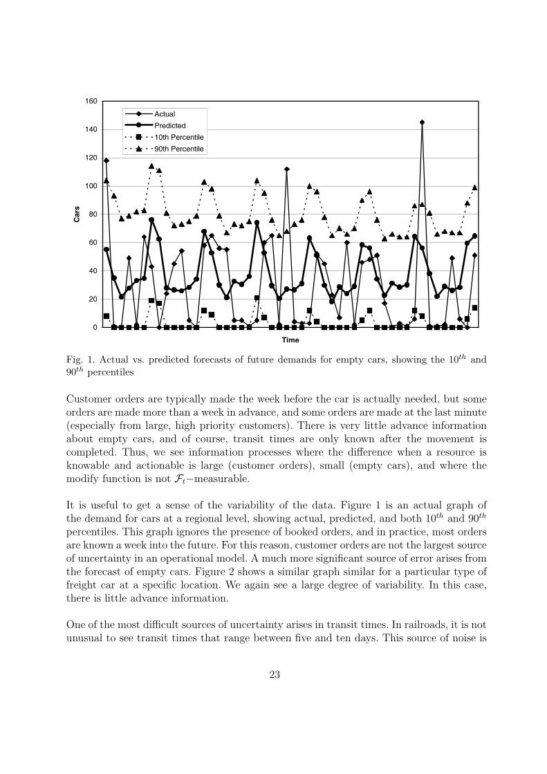
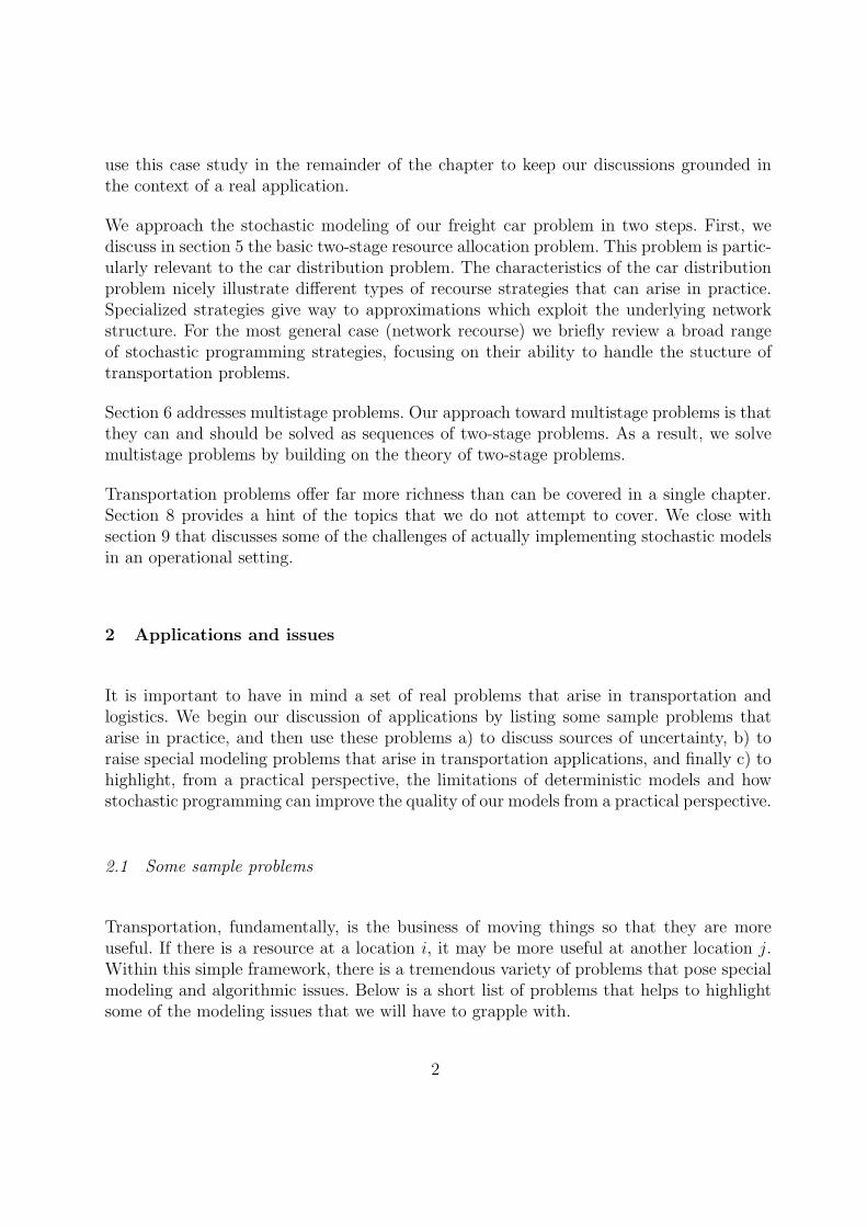
Fig. 1. Actual vs. predicted forecasts of future demands for empty cars, showing the 10th and90th percentiles

Customer orders are typically made the week before the car is actually needed, but someorders are made more than a week in advance, and some orders are made at the last minute(especially from large, high priority customers). There is very little advance informationabout empty cars, and of course, transit times are only known after the movement iscompleted. Thus, we see information processes where the difference when a resource isknowable and actionable is large (customer orders), small (empty cars), and where themodify function is not Ft−measurable.

It is useful to get a sense of the variability of the data. Figure 1 is an actual graph ofthe demand for cars at a regional level, showing actual, predicted, and both 10th and 90th

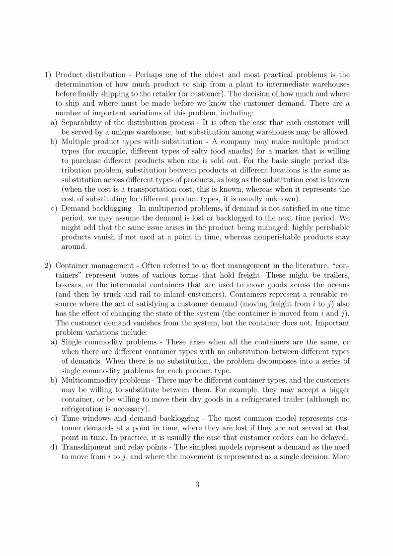
percentiles. This graph ignores the presence of booked orders, and in practice, most ordersare known a week into the future. For this reason, customer orders are not the largest sourceof uncertainty in an operational model. A much more significant source of error arises fromthe forecast of empty cars. Figure 2 shows a similar graph similar for a particular type offreight car at a specific location. We again see a large degree of variability. In this case,there is little advance information.

One of the most difficult sources of uncertainty arises in transit times. In railroads, it is notunusual to see transit times that range between five and ten days. This source of noise is

23

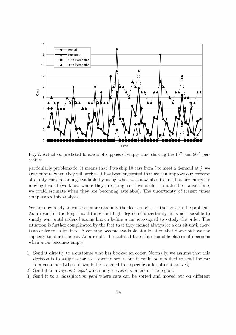
Fig. 2. Actual vs. predicted forecasts of supplies of empty cars, showing the 10th and 90th per-centiles

particularly problematic. It means that if we ship 10 cars from i to meet a demand at j, weare not sure when they will arrive. It has been suggested that we can improve our forecastof empty cars becoming available by using what we know about cars that are currentlymoving loaded (we know where they are going, so if we could estimate the transit time,we could estimate when they are becoming available). The uncertainty of transit timescomplicates this analysis.

We are now ready to consider more carefully the decision classes that govern the problem.As a result of the long travel times and high degree of uncertainty, it is not possible tosimply wait until orders become known before a car is assigned to satisfy the order. Thesituation is further complicated by the fact that they cannot always let a car sit until thereis an order to assign it to. A car may become available at a location that does not have thecapacity to store the car. As a result, the railroad faces four possible classes of decisionswhen a car becomes empty:

1) Send it directly to a customer who has booked an order. Normally, we assume that thisdecision is to assign a car to a specific order, but it could be modified to send the carto a customer (where it would be assigned to a specific order after it arrives).

2) Send it to a regional depot which only serves customers in the region.3) Send it to a classification yard where cars can be sorted and moved out on different

24

trains. A classification yard at a railroad is a major facility and represents a point whereit is easiest to make a decision about a car. From a classification yard, a car may be sentto another classification yard, a regional depot or directly to a customer.

4) Do nothing. This means storing the car at its current location. This is generally notpossible if it just became available at a customer, but is possible if it is at a storagedepot.

Not every car can be immediately assigned to an order, partly because some orders simplyhave not been booked yet, and possibly because there are times of the year when thereare simply more cars than we need. At the same time, one would expect that we do notalways assign a car to a particular order, because not all the available cars are known rightnow. However, there is a strong bias to find an available car that we know about rightnow (even if it is a longer distance from the order) than to use a car that might becomeavailable later.

5 The two-stage resource allocation problem

We start with the two-stage problem because it is fundamental to multistage problems,and because some important algorithmic issues can be illustrated with minimum complex-ity. It should not be surprising that we are going to solve multistage problems basicallyby applying our two-stage logic over and over again. For this reason, it is particularlyimportant that we be able to understand the two-stage problem very well.

We begin our presentation in section 5.1 with a brief discussion of our notational style.Two-stage problems are relatively simple, and it is common to use notational shortcuts totake advantage of this simplicity. The result, however, is a formulation that is difficult togeneralize to harder problems. 5.2 summarizes some of the basic notation used specificallyfor the car distribution problem. We introduce our first model in section 5.3 which presentsmodels that are in practice today. We then provide three levels of generalization on thisbasic model. The first (section 5.4) introduces uncertainty without any form of substitution,producing the classical “stochastic programming with simple recourse” formulation. Thesecond models the effect of regional depots (section 5.5), which produces a separable two-stage problem which can be solved using specialized techniques. The last model considersclassification yards which requires modeling general substitution (section 5.6), and bringsinto play general two-stage stochastic programming, although we take special advantageof the underlying network structure. Finally, section 5.7 discusses some of the issues thatarise for problems with large attribute spaces.

25

5.1 Notational style

One of the more subtle modeling challenges is the indexing of time. In a two stage prob-lem, this is quite simple. Often, we will let x denote an initial decision, followed by newinformation (say, ξ), after which there is a second decision (perhaps denoted by y) that isallowed to use the information in the random variable ξ.

This is very simple notation, but does not generalize to multistage problems. Unfortu-nately, there is not a completely standard notation for indexing activities over time. Theproblem arises because there are two processes: the information process, and the physicalprocess. Within the information process, there is exogenous information, and the processof making decisions (which can be viewed as endogenously controllable information). Inmany problems, and especially true of transportation, there is often a lag between theinformation process (when we know about an activity) and the physical process (when ithappens). (We ignore a third process, which is the flow of financial rewards, such as billinga customer for an activity at the end of a month.)

In the operations research literature, it is common to use notation such as xt to representthe vector of flows occurring (or initiating) in time t. This is virtually always the casein a deterministic model (which ignores completely the time staging of information). Instochastic models, it is more common (although not entirely consistent) to index a variablebased on the information content. In our presentation, we uniformly adopt the notationthat any variable indexed by time t is able to use the exogenous information up throughand including time t (that is, ξ0, ξ1, . . . , ξt). If xt is a decision made in time t, then itis also allowed to see the information up through time t. It is often useful to think ofξt as information arriving “during time period t” whereas the decision xt is a functiondetermined at the end of time period t.

We treat t = 0 as the starting point in time. The discrete time t = 1 refers to the timeinterval between 0 and 1. As a result, the first set of new information would be ξ1. If we letS0 be our initial state variable, we can make an initial decision using only this information,which would be designated x0. A decision made using ξ1 would be designated x1.

There may be a lag between when the information arrives about an activity and whenthe activity happens. It is tempting, for example, to let Dt be the demands that arrivein period t, but we would let Dt be the orders that become known in time period t. Ifa customer calls in an order during time interval t which has to be served during timeinterval t′, then we would denote this variable by Dtt′ . Similarly, we might make a decisionin time period t to serve an order in time period t′; such an activity would be indexed byxtt′ .

26

A more subtle notational issue arises in the representation of state variables. Here wedepart from standard notation in stochastic programming which typically avoids an explicitdefinition of a state variable (the “state” of the system going into time t is the vector ofdecisions made in the previous period xt−1). In resource allocation problems, vectors such asxt can have a very large number of dimensions. These decisions produce future inventoriesof resources which can be represented using much lower dimensional state variables. Inpractice, these are much easier to work with.

It is common in multistage problems to let St be the state of the system at the beginningof time period t, after which a decision is made, followed by new information. Followingour convention, St would represent the state after the new information becomes knownin period t, but it is ambiguous whether this represents the state of the system before orafter a decision has been made. It is most common in the writing of optimality equationsto define the state of the system to be all the information needed to make the decisionxt. However, for computational reasons, it is often useful to work in terms of the state ofthe system immediately after a decision has been made. If we let S+

t be the complete statevariable, giving all the information needed to make a decision, and let St be the state ofthe system immediately after a decision is made, the history of states, information anddecisions up through time t would be written:

ht = S+0 , x0, S0, ξ1, S

+1 , x1, S1, ξ2, S

+2 , x2, S2, . . . , ξt, S

+t , xt, St, . . . (7)

We sometimes refer to St as the incomplete state variable, because it does not includethe information ξt+1 needed to determine the decision xt+1. For reasons that are madeclear later (see section 6.2), we find it more useful to work in terms of the incompletestate variable St (and hence use the more cumbersome notation S+

t for the complete statevariable).

In this section, we are going to focus on two-stage problems, which consist of two sets ofdecision vectors (the initial decision, and the one after new information becomes known).We do not want to use two different variables (say, x and y) since this does not generalizeto multistage problems. It is tempting to want to use x1 and x2 for the first and secondstage, but we find that the sequencing in equation (7) better communicates the flow ofdecisions and information. As a result, x0 is our “first” stage decision while x1 is our secondstage decision.

27

5.2 Modeling the car distribution problem

Given the complexity of the problem, the simplicity of the models in engineering practiceis amazing. As of this writing, we are aware of two basic classes of models in use in NorthAmerica: myopic models, which match available cars to orders that have already beenbooked into the system, and models with deterministic forecasts, which add to the setof known orders additional orders that have been forecasted. We note that the railroadthat uses a purely myopic model is also characterized by long distances, and probablyhas customers which, in response to the long travel times, book farther in advance (bycontrast, there is no evidence that even a railroad with long transit times has any moreadvance information on the availability of empty cars). These models, then, are basicallytransportation problems, with available cars on the left side of the network and known(and possibly forecasted) orders on the right side.

The freight division of the Swedish National Railroad uses a deterministic time-space net-work to model the flows of loaded and empty cars and explicitly models the capacitiesof trains. However, it appears that the train capacity constraints are not very tight, sim-plifying the problem of forecasting the flows of loaded movements. Also, since the modelis a standard, deterministic optimization formulation, a careful model of the dynamics ofinformation has not been presented, nor has this data been analyzed.

The car distribution problem involves moving cars between the locations that handle cars,store cars and serve customers. We represent these using:

Ic = Set of locations representing customers.Ird = Set of locations representing regional depots.Icl = Set of locations representing classification yards.

It is common to represent the “state” of a car by its location, but we use our more generalattribute vector notation since it allows us to handle issues that arise in practice (andwhich create special algorithmic challenges for the stochastic programming community):

Ac = The set of attributes of the cars.Ao = The set of attributes of an order, including the number of days into the future on

which the order should be served (in our vocabulary, its actionable time).Rc

t,at′ = The number of cars with attribute a that we know about at time t that will be availableat time t′. The attribute vector includes the location of the car (at time t′) as well asits characteristics.

Rot,at′ = The vector of car orders with attribute a ∈ Ao that we know about at time t which

are needed at time t′.

28

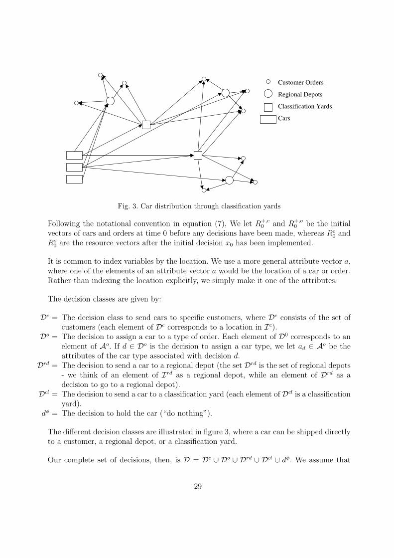
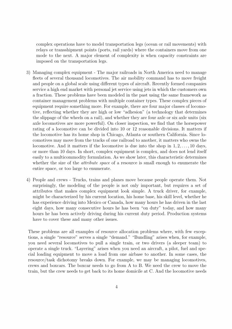
Fig. 3. Car distribution through classification yards

Following the notational convention in equation (7), We let R+,c0 and R+,o

0 be the initialvectors of cars and orders at time 0 before any decisions have been made, whereas Rc

0 andRo

0 are the resource vectors after the initial decision x0 has been implemented.

It is common to index variables by the location. We use a more general attribute vector a,where one of the elements of an attribute vector a would be the location of a car or order.Rather than indexing the location explicitly, we simply make it one of the attributes.

The decision classes are given by:

Dc = The decision class to send cars to specific customers, where Dc consists of the set ofcustomers (each element of Dc corresponds to a location in Ic).

Do = The decision to assign a car to a type of order. Each element of D0 corresponds to anelement of Ao. If d ∈ Do is the decision to assign a car type, we let ad ∈ Ao be theattributes of the car type associated with decision d.

Drd = The decision to send a car to a regional depot (the set Drd is the set of regional depots- we think of an element of Ird as a regional depot, while an element of Drd as adecision to go to a regional depot).

Dcl = The decision to send a car to a classification yard (each element of Dcl is a classificationyard).

dφ = The decision to hold the car (“do nothing”).

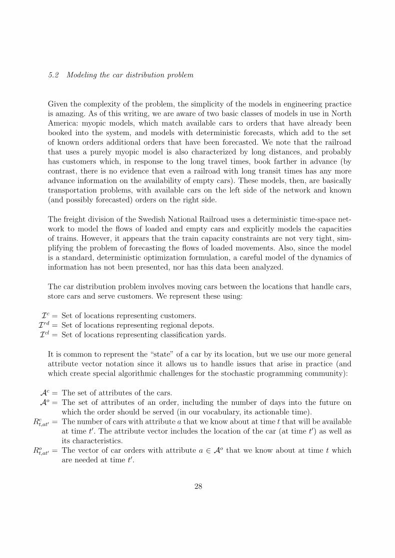
The different decision classes are illustrated in figure 3, where a car can be shipped directlyto a customer, a regional depot, or a classification yard.

Our complete set of decisions, then, is D = Dc ∪ Do ∪ Drd ∪ Dcl ∪ dφ. We assume that

29

we only act on cars (cars are the only active resource class, whereas orders are referredto as a passive resource class). We could turn orders into an active resource class if weallowed them to move without a car (this would arise in practice through outsourcing oftransportation). Of these, decisions in Do are constrained by the number of orders thatare actually available. As before, we let xtad be the number of times that we apply decisiond to a car with attribute a given what we know at time t.

The contribution function is:

ctad = The contribution from assigning a car with attribute a to an order for cars of typed ∈ Do, given what we know at time t. If d ∈ Do, then we assume that the contributionis a “reward” for satisfying a customer order, minus the costs of getting the car tothe order. For all other decision classes, the contributions are the negative costs fromcarrying out the decision.

Since all orders have to be satisfied, it is customary to formulate these models in termsof minimizing costs: the cost of moving a car from its current location to the customer,and the “cost” of assigning a particular type of car to satisfy the order. Since rail costsare extremely complex (what is the marginal cost of moving an additional empty car ona train?), all costs are basically surrogates. The transportation cost could be a time ordistance measurement. If we satisfy the customer order with the correct car type, thenthe car type cost might be zero, with higher costs (basically, penalties) for substitutingdifferent car types to satisfy an order. Just the same, we retain our maximization frameworkbecause this is more natural as we progress to more general models (where we maximize“profits” rather than minimize costs).

5.3 Engineering practice - Myopic and deterministic models

The most basic model used in engineering practice is a myopic model, which means thatwe only act on the vectors Rc

0t′ and Ro0t′ (we believe that in practice, it is likely that

companies even restrict the vector of cars to those that are actionable now, which meansRc

00). We only consider decisions based on what we know now (x0ad), and costs that canbe computed based on what we know now (c0ad). This produces the following optimizationproblem:

minx

∑a∈A

∑d∈D

c0adx0ad (8)

subject to:

30

∑d∈D

x0ad =Rc0a a ∈ A (9)

∑a∈A

x0ad≤Ro0ad

d ∈ Do (10)

x0ad ∈ Z+ (11)

Equation (10) restricts the total assignment of all car types to a demand type ad, d ∈ Do,by the total known demand for that car type across all actionable times. The model allowsa car to be assigned to a demand, even though the car may arrive after the time that theorder should have been served. Penalties for late service are assumed to be captured inc0ad.

It is easy to pick this model apart. First, the model will never send a car to a regionaldepot or classification yard (unless there happens to be a customer order at precisely thatlocation). Second, the model will only send a car to an order that is known. Thus, wewould not take a car that otherwise has nothing to do and begin moving to a locationwhich is going to need the car with a high probability. Even worse, the model may move acar to an order which has been booked, when it could have been moved to a much closerlocation where there probably will be an order (but one has not been booked as yet). Ifthere are more cars than orders, then the model provides almost no guidance as to wherecars should be moved in anticipation of future orders,

Amidst these weaknesses are some notable strengths. First, the model is simple to for-mulate and solve using commercial solvers. Second, the model handles all three types ofsubstitution extremely easily (especially important is substitution across time, somethingthat models often struggle with). But, perhaps the most important feature is that the so-lution is easy to understand. The most overlooked limitation of more sophisticated modelsis that their solutions are hard to understand. If the data were perfect, then we wouldargue that the user should simply trust the model, but the limitations of the data precludesuch a casual response.

The first generalization used in practice is to include forecasts of future orders, which wewould represent using the vector Ro

tt′ for t ∈ T ph, where T ph is the set of time periods inour planning horizon. The details of the process of forecasting future orders are, of course,not documented. The process of forecasting would generally have to be made at some levelof aggregation (daily/weekly, customer level or regionl, and the car class). Particularlytricky is handling the time staging of orders. If a forecast is generated for a particular timet′ in the future (using, for example, standard time series forecasting techniques applied toa historical dataset showing customer orders by time period), then we would be forecastingthe total orders for time t′, and then adding in the orders to be satisfied at time t′ that areknown now. We assume that we have a forecast Ro

tt′ representing the orders that would beplaced at time t to be satisfied at time t′.

31

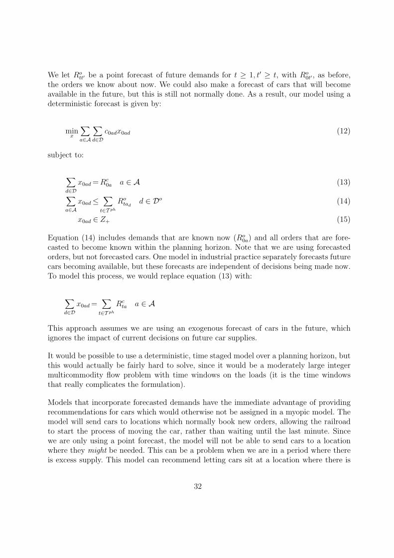
We let Rott′ be a point forecast of future demands for t ≥ 1, t′ ≥ t, with Ro

0t′ , as before,the orders we know about now. We could also make a forecast of cars that will becomeavailable in the future, but this is still not normally done. As a result, our model using adeterministic forecast is given by:

minx

∑a∈A

∑d∈D

c0adx0ad (12)

subject to:

∑d∈D

x0ad =Rc0a a ∈ A (13)

∑a∈A

x0ad≤∑

t∈T ph

Rotad

d ∈ Do (14)

x0ad ∈ Z+ (15)

Equation (14) includes demands that are known now (Ro0a) and all orders that are fore-

casted to become known within the planning horizon. Note that we are using forecastedorders, but not forecasted cars. One model in industrial practice separately forecasts futurecars becoming available, but these forecasts are independent of decisions being made now.To model this process, we would replace equation (13) with:

∑d∈D

x0ad =∑

t∈T ph

Rcta a ∈ A

This approach assumes we are using an exogenous forecast of cars in the future, whichignores the impact of current decisions on future car supplies.

It would be possible to use a deterministic, time staged model over a planning horizon, butthis would actually be fairly hard to solve, since it would be a moderately large integermulticommodity flow problem with time windows on the loads (it is the time windowsthat really complicates the formulation).

Models that incorporate forecasted demands have the immediate advantage of providingrecommendations for cars which would otherwise not be assigned in a myopic model. Themodel will send cars to locations which normally book new orders, allowing the railroadto start the process of moving the car, rather than waiting until the last minute. Sincewe are only using a point forecast, the model will not be able to send cars to a locationwhere they might be needed. This can be a problem when we are in a period where thereis excess supply. This model can recommend letting cars sit at a location where there is

32

absolutely no chance of them being used, rather than moving them to a location wherethey might be used.

Our model does not include forecasts of empty cars. The common rationale for leavingthese forecasts out is that they are so uncertain (it is not unusual for practitioners toignore information which cannot be reasonably approximated by a point forecast). It alsoignores many other operational issues such as train capacities (which we have alreadyidentified to be highly uncertain), yard capacities (which determines how many cars canbe stored at a location) or the value of cars at the end of the horizon (which we couldovercome with a multistage model).

There are a number of limitations of these simple models, but we would argue that a seriouspractical limitation is that the model will never recommend sending a car to a regionaldepot or classification yard. In one application with which we are familiar, the model willrecommend sending a car to a particular customer (perhaps to serve a forecasted order).In the process of routing the car to the customer, the car will have to go through a regionaldepot. The railroad will then route the car to the depot, reoptimizing the assignment ofthe car to new orders as they become available. This is a highly heuristic way of accountingfor uncertainty.

5.4 No substitution - a simple recourse model

Our first effort o incorporate uncertainty is a simple recourse model where we replace thedecision class to assign cars to a specific order and instead allow us to send cars to aparticular customer (or equivalently, to a customer location). The difference is that if acustomer only places one order, then in the first model we can only send him one car. Inour simple recourse model, we may send more cars to the customer location at time t thanhas been ordered at time t′ in the hopes that new orders will come in later. For this case,we define:

Rot,ct′ = The number of orders for customer c that we first learn about at time t that are

actionable (must be served) at time t′.Ro

t,c = All the orders for customer c known at time t.= (Ro

t,ct′)t′≥t.

Of course, Ro0 are the orders we know about now, while (Ro

t )t>0 are the forecasted ordersfor the future. Unlike our first models, we are now going to explicitly model the uncertaintyin the forecast of future orders. Looking at equation (14), we see that we only need thetotal forecast of future demands. For this reason, it is simpler to define:

33

Ro1,c =

∑t∈T ph\0

∑t′∈T ph\0

Rot,ct′

Ro1c is a random variable representing all “future” demands, which would be derived from a

forecasting model. Note that we have aggregated not only on all orders that would becomeknown in the future (t), but we have also aggregated across the dates when the orderswould need to be satisfied (t′). Let:

Rc0,id

= The number of cars (indicated by the superscript c) sent to customer id, d ∈ Dc, wherethe decision is made at time 0 but the cars can be used at time 1 (the second stage).

=∑

a∈A x0ad

The decisions x0ad must be made before the orders (Roti)t>0 become known. In our simple

recourse model, we assume that a car sent to customer c cannot then, at a later time, besent to another customer. It is either used to satisfy an order (within our planning horizon)or it sits idle. Let:

coi = The (positive) contribution from satisfying an order for customer i ∈ Ic.chi = The contribution (typically negative) from sending a car to customer i and then having

it sit.

Now let:

xo1i = The number of cars assigned to serve an order (after they arrive at customer i).xh

1i = The number of cars that are held at customer i.

xo1 and xh

1 are random variables defined by:

xo1c(R

c0,c, R

o1c(ω)) = minRc

0,c, Ro1c(ω)

xh1c(R

c0,c, R

o1c(ω)) = max0, Rc

0,c − Ro1c(ω)

We should note that our choices for xo1c(R

c0,c, R

o1c(ω)) and xh

1c(Rc0,c, R

o1c(ω)) seem a bit

obvious, but they are in fact the result of a trivial optimization problem.

Rc0,c1 is a function of the first stage decisions x0. Given x0, the expected second stage

reward is given by:

34

C0,1(Rc0(x0)) = Expected costs using the information available in time period 0

that would be incurred in time period 1.

=E

∑c∈Ic

(cocx

o1c(R

c0c(x0), R

o1c) + chcx

h1c(R

c0c, R

o1c)

)

=∑c∈Ic

(C0,c1(R

c0c(x0))

)The functions C0,c1(R

c0c) are concave. If the random demands are discrete, then it is also

possible to show that C0,c1(Rc0c) is piecewise linear, concave, with the breakpoints at in-

teger values of Rc0c. Since these functions are computed as expectations of scalar random

variables, computing them is quite easy once the distribution of demands is known. Ofcourse, forecasting future demands is in practice fairly tricky, primarily because of theprocess of customers booking orders in advance.

We can now formulate our problem as follows:

minx0

c0x0 + C0,1(R

c0(x0))

(16)

subject to:

∑d∈D

x0ad =R+,c0a a ∈ A (17)

∑a∈A

x0ad≤R+,o0ad

d ∈ Do (18)

x0ad ∈ Z+ (19)

This is a convex nonlinear programming problem with network constraints. If the demandsare discrete, producing piecewise-linear concave reward functions for each shipper, thenwe can use a standard trick for converting these problems into pure networks, as shown infigure 4.

5.5 Shipping to regional depots - a separable recourse model

The major weakness of the simple recourse model is that it does not capture the ability ofthe railroad to send cars to a regional depot, and then wait until the last minute to sendcars from the depot to the customer. In fact, it is generally not possible to send a car toa customer unless the customer has specifically asked for the car. A more realistic modelis to assume that the car has been sent to a local yard (which we refer to as a regionaldepot) where it is stored waiting for customers.

35

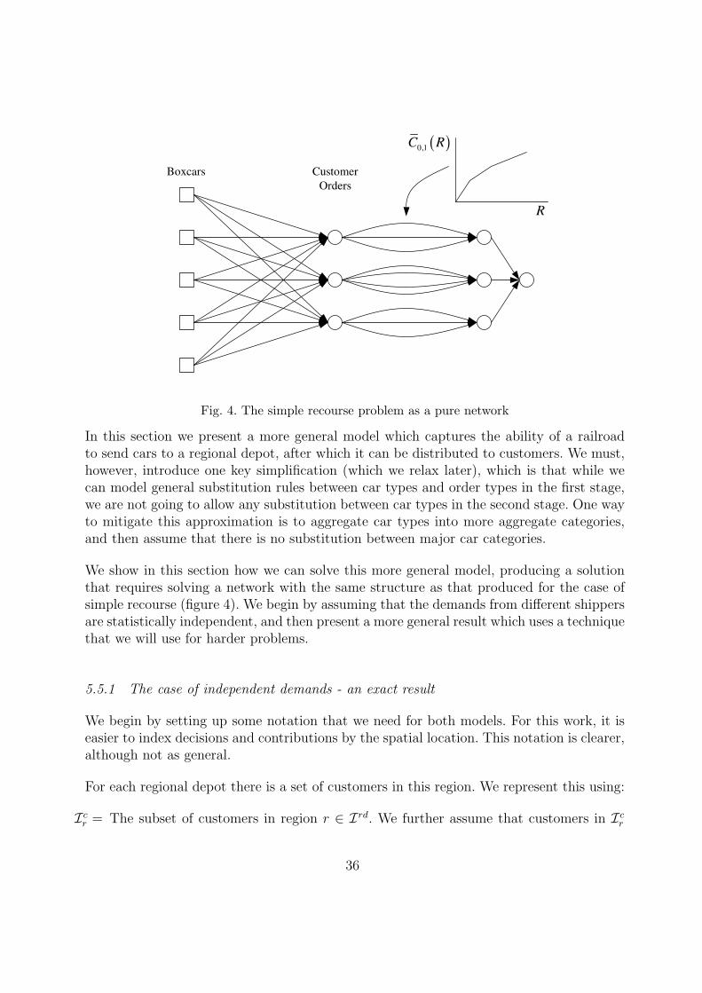
Fig. 4. The simple recourse problem as a pure network

In this section we present a more general model which captures the ability of a railroadto send cars to a regional depot, after which it can be distributed to customers. We must,however, introduce one key simplification (which we relax later), which is that while wecan model general substitution rules between car types and order types in the first stage,we are not going to allow any substitution between car types in the second stage. One wayto mitigate this approximation is to aggregate car types into more aggregate categories,and then assume that there is no substitution between major car categories.

We show in this section how we can solve this more general model, producing a solutionthat requires solving a network with the same structure as that produced for the case ofsimple recourse (figure 4). We begin by assuming that the demands from different shippersare statistically independent, and then present a more general result which uses a techniquethat we will use for harder problems.

5.5.1 The case of independent demands - an exact result

We begin by setting up some notation that we need for both models. For this work, it iseasier to index decisions and contributions by the spatial location. This notation is clearer,although not as general.

For each regional depot there is a set of customers in this region. We represent this using:

Icr = The subset of customers in region r ∈ Ird. We further assume that customers in Ic

r

36

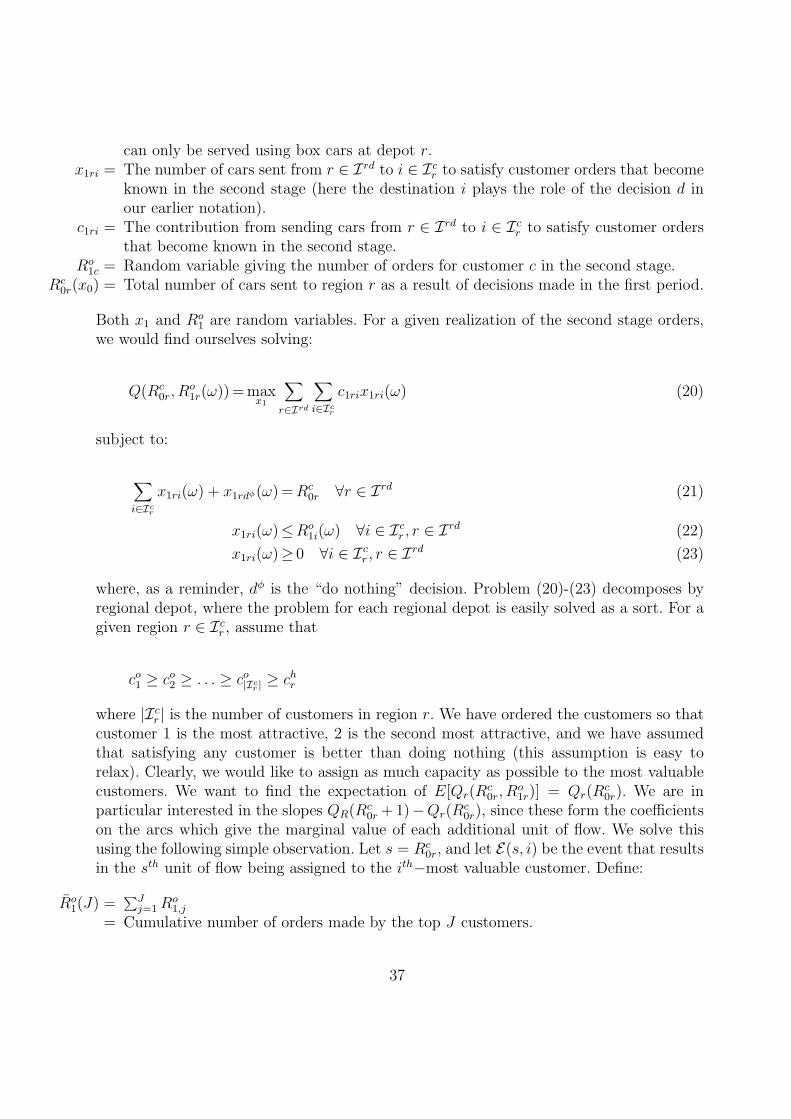
can only be served using box cars at depot r.x1ri = The number of cars sent from r ∈ Ird to i ∈ Ic

r to satisfy customer orders that becomeknown in the second stage (here the destination i plays the role of the decision d inour earlier notation).

c1ri = The contribution from sending cars from r ∈ Ird to i ∈ Icr to satisfy customer orders

that become known in the second stage.Ro

1c = Random variable giving the number of orders for customer c in the second stage.Rc

0r(x0) = Total number of cars sent to region r as a result of decisions made in the first period.

Both x1 and Ro1 are random variables. For a given realization of the second stage orders,

we would find ourselves solving:

Q(Rc0r, R

o1r(ω)) = max

x1

∑r∈Ird

∑i∈Ic

r

c1rix1ri(ω) (20)

subject to:

∑i∈Ic

r

x1ri(ω) + x1rdφ(ω) =Rc0r ∀r ∈ Ird (21)

x1ri(ω)≤Ro1i(ω) ∀i ∈ Ic

r , r ∈ Ird (22)

x1ri(ω)≥ 0 ∀i ∈ Icr , r ∈ Ird (23)

where, as a reminder, dφ is the “do nothing” decision. Problem (20)-(23) decomposes byregional depot, where the problem for each regional depot is easily solved as a sort. For agiven region r ∈ Ic

r , assume that

co1 ≥ co2 ≥ . . . ≥ co|Icr | ≥ chr

where |Icr | is the number of customers in region r. We have ordered the customers so that

customer 1 is the most attractive, 2 is the second most attractive, and we have assumedthat satisfying any customer is better than doing nothing (this assumption is easy torelax). Clearly, we would like to assign as much capacity as possible to the most valuablecustomers. We want to find the expectation of E[Qr(R

c0r, R

o1r)] = Qr(R

c0r). We are in

particular interested in the slopes QR(Rc0r + 1)−Qr(R

c0r), since these form the coefficients

on the arcs which give the marginal value of each additional unit of flow. We solve thisusing the following simple observation. Let s = Rc

0r, and let E(s, i) be the event that resultsin the sth unit of flow being assigned to the ith−most valuable customer. Define:

Ro1(J) =

∑Jj=1R

o1,j

= Cumulative number of orders made by the top J customers.

37

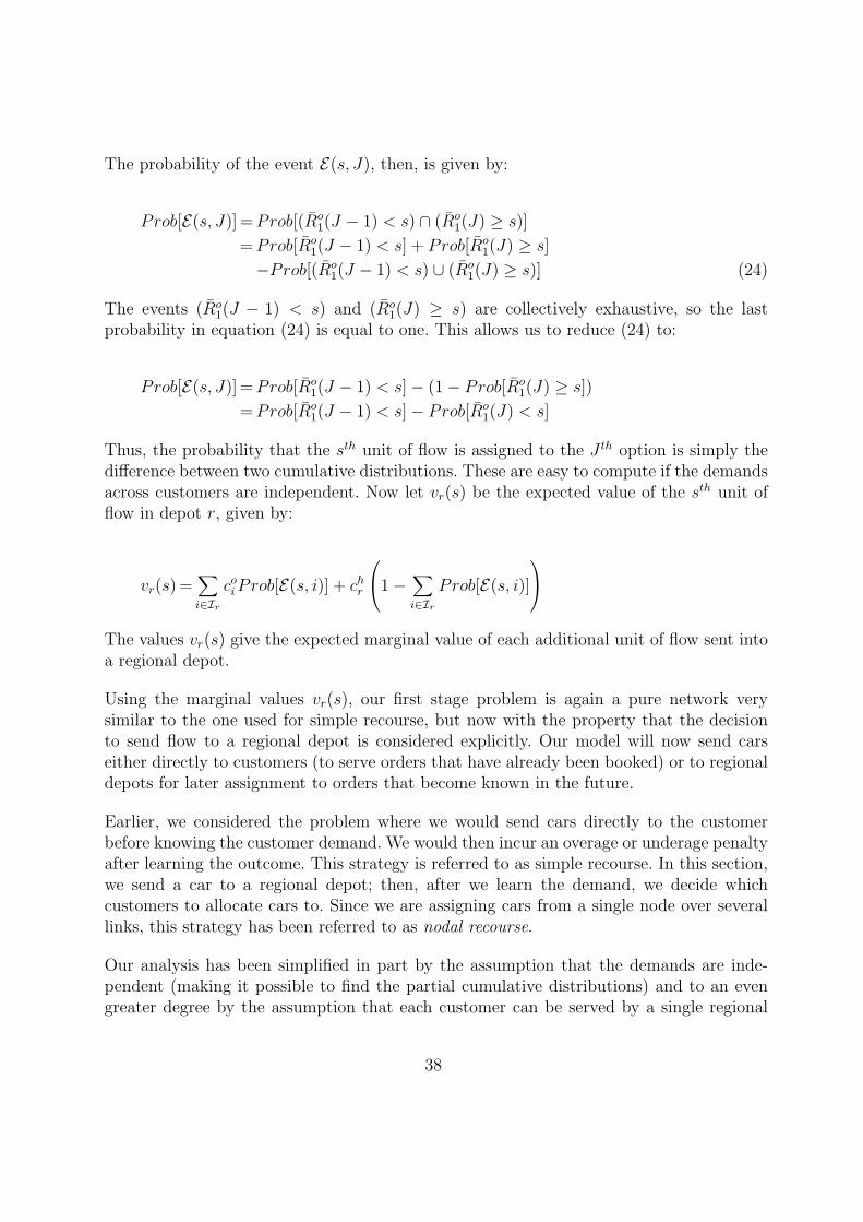
The probability of the event E(s, J), then, is given by:

Prob[E(s, J)] =Prob[(Ro1(J − 1) < s) ∩ (Ro

1(J) ≥ s)]

=Prob[Ro1(J − 1) < s] + Prob[Ro

1(J) ≥ s]

−Prob[(Ro1(J − 1) < s) ∪ (Ro

1(J) ≥ s)] (24)

The events (Ro1(J − 1) < s) and (Ro

1(J) ≥ s) are collectively exhaustive, so the lastprobability in equation (24) is equal to one. This allows us to reduce (24) to:

Prob[E(s, J)] =Prob[Ro1(J − 1) < s]− (1− Prob[Ro

1(J) ≥ s])

=Prob[Ro1(J − 1) < s]− Prob[Ro

1(J) < s]

Thus, the probability that the sth unit of flow is assigned to the J th option is simply thedifference between two cumulative distributions. These are easy to compute if the demandsacross customers are independent. Now let vr(s) be the expected value of the sth unit offlow in depot r, given by:

vr(s) =∑i∈Ir

coiProb[E(s, i)] + chr

1−∑i∈Ir

Prob[E(s, i)]

The values vr(s) give the expected marginal value of each additional unit of flow sent intoa regional depot.

Using the marginal values vr(s), our first stage problem is again a pure network verysimilar to the one used for simple recourse, but now with the property that the decisionto send flow to a regional depot is considered explicitly. Our model will now send carseither directly to customers (to serve orders that have already been booked) or to regionaldepots for later assignment to orders that become known in the future.

Earlier, we considered the problem where we would send cars directly to the customerbefore knowing the customer demand. We would then incur an overage or underage penaltyafter learning the outcome. This strategy is referred to as simple recourse. In this section,we send a car to a regional depot; then, after we learn the demand, we decide whichcustomers to allocate cars to. Since we are assigning cars from a single node over severallinks, this strategy has been referred to as nodal recourse.

Our analysis has been simplified in part by the assumption that the demands are inde-pendent (making it possible to find the partial cumulative distributions) and to an evengreater degree by the assumption that each customer can be served by a single regional

38

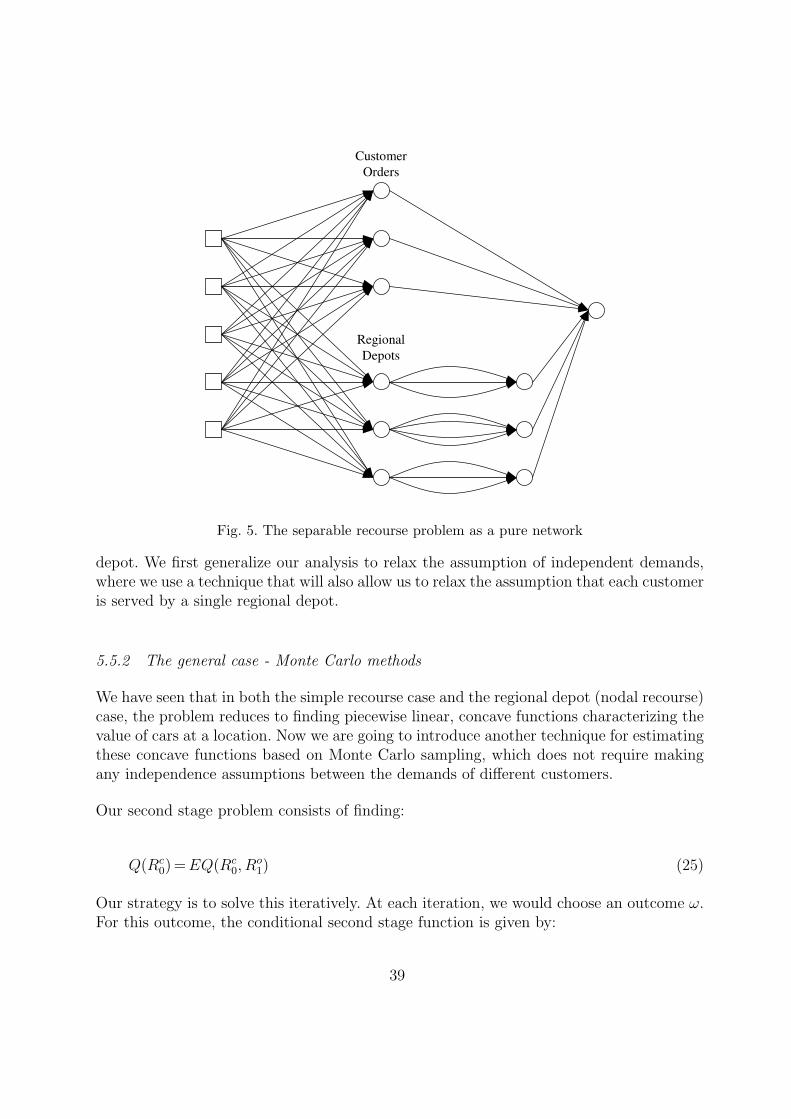
Fig. 5. The separable recourse problem as a pure network

depot. We first generalize our analysis to relax the assumption of independent demands,where we use a technique that will also allow us to relax the assumption that each customeris served by a single regional depot.

5.5.2 The general case - Monte Carlo methods

We have seen that in both the simple recourse case and the regional depot (nodal recourse)case, the problem reduces to finding piecewise linear, concave functions characterizing thevalue of cars at a location. Now we are going to introduce another technique for estimatingthese concave functions based on Monte Carlo sampling, which does not require makingany independence assumptions between the demands of different customers.

Our second stage problem consists of finding:

Q(Rc0) =EQ(Rc

0, Ro1) (25)

Our strategy is to solve this iteratively. At each iteration, we would choose an outcome ω.For this outcome, the conditional second stage function is given by:

39

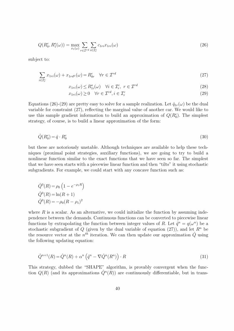
Q(Rc0, R

o1(ω)) = max

x1(ω)

∑r∈Ird

∑i∈Ic

r

c1rix1ri(ω) (26)

subject to:

∑i∈Ic

r

x1ri(ω) + x1rdφ(ω) =Rc0r ∀r ∈ Ird (27)

x1ri(ω)≤Ro1i(ω) ∀i ∈ Ic

r , r ∈ Ird (28)

x1ri(ω)≥ 0 ∀r ∈ Ird, i ∈ Icr (29)

Equations (26)-(29) are pretty easy to solve for a sample realization. Let q1r(ω) be the dualvariable for constraint (27), reflecting the marginal value of another car. We would like touse this sample gradient information to build an approximation of Q(Rc

0). The simpleststrategy, of course, is to build a linear approximation of the form:

Q(Rc0) = q ·Rc

0 (30)

but these are notoriously unstable. Although techniques are available to help these tech-niques (proximal point strategies, auxiliary functions), we are going to try to build anonlinear function similar to the exact functions that we have seen so far. The simplestthat we have seen starts with a piecewise linear function and then “tilts” it using stochasticsubgradients. For example, we could start with any concave function such as:

Q0(R) = ρ0

(1− e−ρ1R

)Q0(R) = ln(R + 1)

Q0(R) =−ρ0(R− ρ1)2

where R is a scalar. As an alternative, we could initialize the function by assuming inde-pendence between the demands. Continuous functions can be converted to piecewise linearfunctions by extrapolating the function between integer values of R. Let qn = q(ωn) be astochastic subgradient of Q (given by the dual variable of equation (27)), and let Rn bethe resource vector at the nth iteration. We can then update our approximation Q usingthe following updating equation:

Qn+1(R) = Qn(R) + αn(qn −∇Qn(Rn)

)·R (31)

This strategy, dubbed the “SHAPE” algorithm, is provably convergent when the func-tion Q(R) (and its approximations Qn(R)) are continuously differentiable, but in trans-

40

portation, we are typically managing discrete resources, and we are interested in integersolutions.

When we are using piecewise linear functions, we can get an even better estimate by usingleft and right gradients of Q(Rc

0, Ro1(ω)) rather than a simple subgradient. Let qn+ and

qn− be the right and left gradients, respectively, of Q(Rc0, R

o1(ω)). Then we can perform a

two-sided update using:

Qn+1(R) =

Qn(R) + αn(qn+ −∇Qn(Rn)

)·R R ≥ Rn

Qn(R) + αn(qn− −∇Qn(Rn)

)·R R < Rn

(32)

There is another class of strategies that we refer to broadly as structured adaptive func-tional estimators (or “SAFE” algorithms). In our problem, we are trying to estimatepiecewise linear, concave functions which can be represented by a sequence of slopes thatare decreasing monotonically. At each iteration, we obtain stochastic gradients that allowus to update estimates of these slopes, but it is important to maintain the concavity ofour function or, equivalently, the monotonicity of the slopes. We briefly review two strate-gies for performing this estimation. The first is referred to as a leveling technique sinceviolations of concavity are fixed by leveling the estimates of the slopes (see below). Thesecond is called a separable, projective approximation routine (SPAR), since we maintainmonotonicity in the slopes by performing a projection of the updated function onto thespace of concave functions.

Both approaches begin by representing the piecewise linear function Q(R) by its slopes asfollows. Let:

qr =Q(r + 1)−Q(r)

be the right derivative of Q(R) at R = r. We can then write:

Q(R) =Q(0) +R−1∑r=0

qr

Let qnr be an estimate of qr at iteration n. As before, let qn be a stochastic gradient of

Q at iteration n, and assume they have the property that E[qnr ] = qr. Assume that at

iteration n we sample r = Rn(ω). We could estimate the slopes using the simple updatingequations:

41

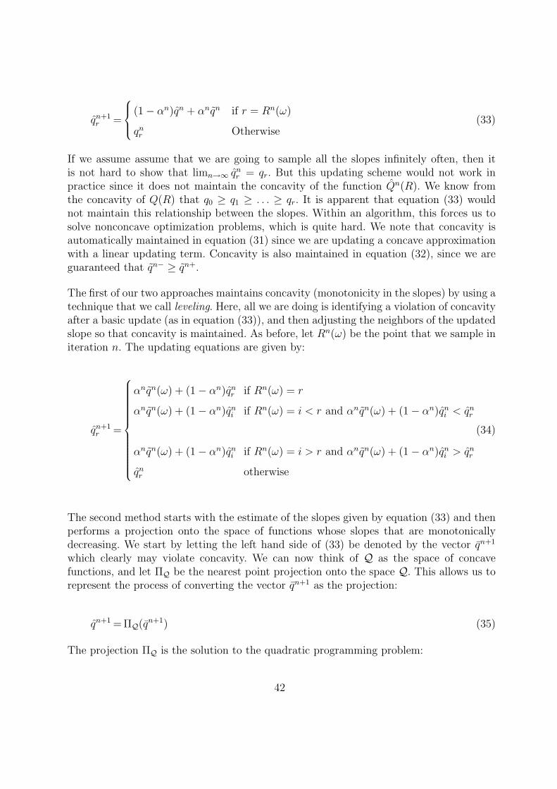
qn+1r =

(1− αn)qn + αnqn if r = Rn(ω)

qnr Otherwise

(33)

If we assume assume that we are going to sample all the slopes infinitely often, then itis not hard to show that limn→∞ qn

r = qr. But this updating scheme would not work inpractice since it does not maintain the concavity of the function Qn(R). We know fromthe concavity of Q(R) that q0 ≥ q1 ≥ . . . ≥ qr. It is apparent that equation (33) wouldnot maintain this relationship between the slopes. Within an algorithm, this forces us tosolve nonconcave optimization problems, which is quite hard. We note that concavity isautomatically maintained in equation (31) since we are updating a concave approximationwith a linear updating term. Concavity is also maintained in equation (32), since we areguaranteed that qn− ≥ qn+.

The first of our two approaches maintains concavity (monotonicity in the slopes) by using atechnique that we call leveling. Here, all we are doing is identifying a violation of concavityafter a basic update (as in equation (33)), and then adjusting the neighbors of the updatedslope so that concavity is maintained. As before, let Rn(ω) be the point that we sample initeration n. The updating equations are given by:

qn+1r =

αnqn(ω) + (1− αn)qnr if Rn(ω) = r

αnqn(ω) + (1− αn)qni if Rn(ω) = i < r and αnqn(ω) + (1− αn)qn

i < qnr

αnqn(ω) + (1− αn)qni if Rn(ω) = i > r and αnqn(ω) + (1− αn)qn

i > qnr

qnr otherwise

(34)

The second method starts with the estimate of the slopes given by equation (33) and thenperforms a projection onto the space of functions whose slopes that are monotonicallydecreasing. We start by letting the left hand side of (33) be denoted by the vector qn+1

which clearly may violate concavity. We can now think of Q as the space of concavefunctions, and let ΠQ be the nearest point projection onto the space Q. This allows us torepresent the process of converting the vector qn+1 as the projection:

qn+1 = ΠQ(qn+1) (35)

The projection ΠQ is the solution to the quadratic programming problem:

42

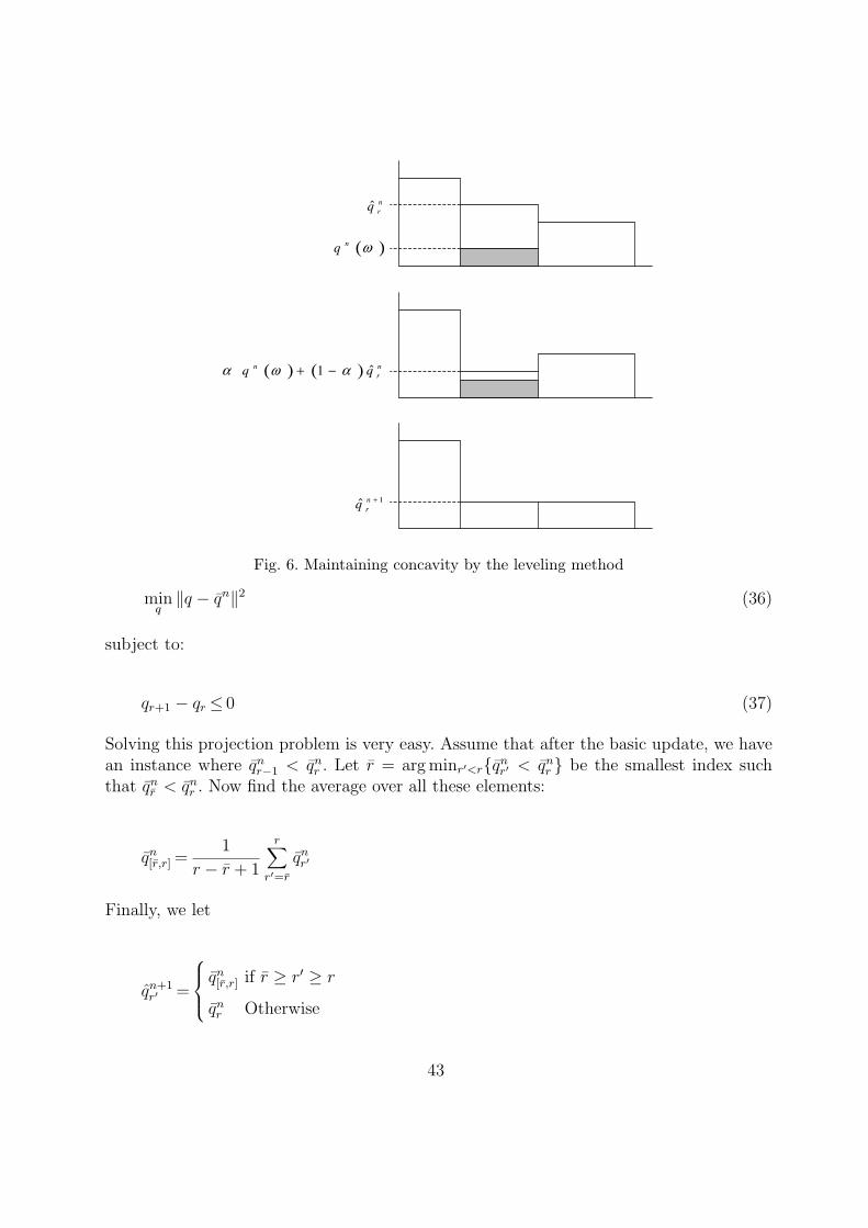
Fig. 6. Maintaining concavity by the leveling method

minq‖q − qn‖2 (36)

subject to:

qr+1 − qr≤ 0 (37)

Solving this projection problem is very easy. Assume that after the basic update, we havean instance where qn

r−1 < qnr . Let r = arg minr′<rqn

r′ < qnr be the smallest index such

that qnr < qn

r . Now find the average over all these elements:

qn[r,r] =

1

r − r + 1

r∑r′=r

qnr′

Finally, we let

qn+1r′ =

qn[r,r] if r ≥ r′ ≥ r

qnr Otherwise

43

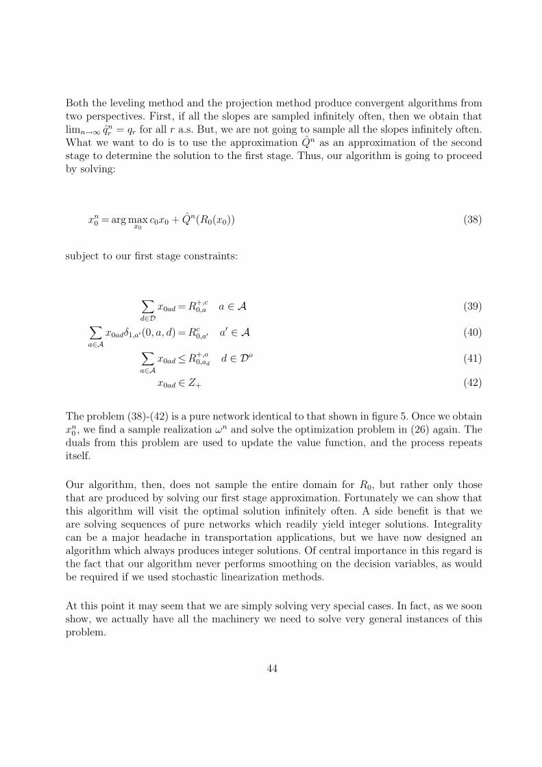
Both the leveling method and the projection method produce convergent algorithms fromtwo perspectives. First, if all the slopes are sampled infinitely often, then we obtain thatlimn→∞ qn

r = qr for all r a.s. But, we are not going to sample all the slopes infinitely often.What we want to do is to use the approximation Qn as an approximation of the secondstage to determine the solution to the first stage. Thus, our algorithm is going to proceedby solving:

xn0 = arg max

x0c0x0 + Qn(R0(x0)) (38)

subject to our first stage constraints:

∑d∈D

x0ad =R+,c0,a a ∈ A (39)

∑a∈A

x0adδ1,a′(0, a, d) =Rc0,a′ a′ ∈ A (40)∑

a∈Ax0ad≤R+,o

0,add ∈ Do (41)

x0ad ∈ Z+ (42)

The problem (38)-(42) is a pure network identical to that shown in figure 5. Once we obtainxn

0 , we find a sample realization ωn and solve the optimization problem in (26) again. Theduals from this problem are used to update the value function, and the process repeatsitself.

Our algorithm, then, does not sample the entire domain for R0, but rather only thosethat are produced by solving our first stage approximation. Fortunately we can show thatthis algorithm will visit the optimal solution infinitely often. A side benefit is that weare solving sequences of pure networks which readily yield integer solutions. Integralitycan be a major headache in transportation applications, but we have now designed analgorithm which always produces integer solutions. Of central importance in this regard isthe fact that our algorithm never performs smoothing on the decision variables, as wouldbe required if we used stochastic linearization methods.

At this point it may seem that we are simply solving very special cases. In fact, as we soonshow, we actually have all the machinery we need to solve very general instances of thisproblem.

44

5.6 Shipping to classification yards - a network recourse model

The next level of generalization is the challenge of working with what we call “classificationyards.” For the purpose of this presentation, we are going to assume that we can send carsfrom classification yards to any customers in the network (for the moment, we are notgoing to allow ourselves to send cars to regional depots, since this would take us past ourbasic two-stage model). For the moment, we are going to continue to assume that once carsreach a classification yard that there is no substitution between car types: if a customerorder is for car type k, then we must provide car type k. But we are going to assume thata single customer can be served from more than one depot.

This problem is known to the stochastic programming community as a two-stage stochasticprogram with network recourse. The reason is that, unlike our previous models, the secondstage is now a general network problem (as opposed to the much simpler problems posedby simple or nodal recourse). Solving a network problem in the second stage is almostas difficult as solving a general linear program, which means that we should consideralgorithms designed for general two-stage stochastic linear programs.

The research community has developed a number of algorithmic strategies over the years.The question of whether an algorithmic strategy works has to be answered in three levels: 1)Does the algorithm appear to work in theory? Does it capture the mathematical propertiesof the problem? 2) Does it produce reasonable numerical results in laboratory experiments?For example, using datasets reflecting specific classes of problems, we would like to know ifit converges quickly, producing stable, high quality solutions. 3) Does it work in practice,producing recommendations that are acceptable to those who have to implement them?

As of the writing of this chapter, there is a strong handle on the theory, but numericaltesting is extremely limited (given the broad diversity of problems). For example, showingthat it works well on car distribution problems for one railroad will not always convinceanother railroad that it will work on their network! Container management problems (intrucking, rail and intermodal applications) come in a variety of sizes and characteristics.The dynamics of short-haul regional truckload carriers are completely different from thoseof long-haul national carriers. Experiments in pure transportation applications do nottell us whether it would work in other resource allocation settings such as supply chainmanagement and distribution problems. And we are not even talking about applicationsoutside of transportation and logistics. In short, each subcommunity (and these can be veryspecialized) needs to see numerical work to demonstrate effectiveness on its own problemclass.

Given the very limited amount of laboratory testing of the different algorithmic strategies(even within general transportation problems), our discussion focuses on the qualities of

45

different algorithms and their potential strengths and weaknesses for our problem. Wecannot definitively state what will and will not work for our problem class, but we candiscuss the qualities of different approaches. In particular, we are interested in the degreeto which a technique allows us to exploit the underlying structure of the transportationproblem. Many transportation problems require integer solutions, and also exhibit near-network structure. Algorithms which allow us to exploit this network structure are morelikely to yield integer solutions from LP relaxations, or at least provide tight LP relaxations.

5.6.1 Scenario methods

Perhaps the best known algorithmic strategy in stochastic programming is scenario pro-gramming, popular because of its conceptual simplicity, generality, and use of general-purpose optimization algorithms. But, its effectiveness for transportation applications isdoubtful.

Let Ω be a (not too large) sample of outcomes (future car orders, future car supplies,as well as travel times). Further let p(ω) be the probability of outcome ω ∈ Ω. We canapproximate our original problem using the method of scenarios:

maxx0,x1

c0x0 +∑ω∈Ω

p(ω)c1x1(ω) (43)

subject to:

First-stage constraints:

∑d∈D

x0ad =Rc0a a ∈ A (44)

∑a∈A

x0ad≤Ro0ad

d ∈ Do (45)∑a∈A

∑d∈Da

x0adδ1,a′(0, a, d)−Rc0,a′1 = 0 a′ ∈ A (46)

x0ad ∈ Z+ a ∈ A, d ∈ D (47)

Second-stage constraints:

46

∑d∈Dc

a

x1ad(ω) + x1adφ(ω) =Rc0,a ∀a ∈ A, ∀ω ∈ Ω (48)

∑a∈A

x1ad(ω)≤Ro1cd

(ω) d ∈ Dc, ∀ω ∈ Ω (49)

x1ad(ω)≥ 0 ∀a ∈ A, d ∈ Dca, ∀ω ∈ Ω (50)

We note that our decision class D only allows us to assign cars to a known order, or toreposition cars to a general or regional depot. As a result, the second stage problem isprimarily one of assigning cars from the general and regional depots to orders that becameknown in the second stage.

Scenario methods have been very popular in financial applications, but we feel that thereare specific characteristics of financial applications that are not shared in transportationapplications, and vice versa. Financial applications are characterized by very complexstochastic processes with high levels of interdependence reflecting the dependence of ran-dom outcomes on a relatively smaller number of common factors. It is easier, then, toreasonably approximate the future with a smaller number of scenarios. Also, financialapplications typically do not have integer variables.

Transportation applications, on the other hand, are characterized by a large number ofrelatively independent random variables. The optimization problems, which are typicallyinteger, are often so large that deterministic problems are hard (although they often haveimbedded network structures). The formulation in (43)-(50) has the effect of taking acomputationally intractable problem and blowing it up into a problem that is many timeslarger. Furthermore, many transportation problems exhibit a natural network structurethat is destroyed by the representation of the second stage problem.

5.6.2 Benders decomposition

Benders decomposition is an appealing algorithm that replaces the very large problemsposed in scenario optimization with sequences of relatively small problems of the form(which we state here as a minimization problem as is standard practice in the literature):

minx0

c0x0 + z (51)

subject to the first stage constraints (44)-(47) which we represent compactly using:

A0x0 =R0 (52)

x0≥ 0 (53)

47

and the constraints:

z − βix0≥αi, ∀ i = 1, ..., n (54)

where βi and αi are generated by solving the dual of the second stage problem, which forcompactness we can write as:

minx1

c1x1(ω)

subject to:

A1x1(ω) =R1(ω) +B0x0

x1(ω)≥ 0

Different algorithms have been proposed for generating cuts. The first algorithm of thisclass is the so-called “L-shaped” decomposition, which works on a finite set of outcomes(which cannot be too large, since we have to solve a linear program for each outcome). Thisconcept was generalized by the stochastic decomposition algorithm which generates cutsfrom a potentially infinite sample space. A sketch of the algorithm is given in figure 7. Thisalgorithm converges almost surely to the optimal solution, but the rate of convergence onpractical applications remains an open question.

The CUPPS algorithm (outlined in figure 8) requires a finite sample space which can bequite large (for example, thousands or tens of thousands of scenarios). The critical step inthe stochastic decomposition is equation (56) which requires smoothing on the coefficientsof the cuts. The critical step in the CUPPS algorithm is equation (57) which requires asimple arithmetic calculation over the entire sample space. Since equation (57) is quitesimple, it is not hard to execute even for tens of thousands of scenarios, but it preventsthe algorithm from ever being applied rigorously to complete sample spaces (for realisticproblems) which can be of the order 1010 or even 10100. From a practical perspective, it isnot clear if this is useful.

We need to keep in mind that Benders decomposition is probably limited (in transportationapplications) to the types of resource allocation problems that we have been considering(since these can be reasonably approximated as continuous linear programs). However,there are unanswered experimental questions even for this special problem class. First,there is the usual issue of rate of convergence. Real car distribution problems may haveover 100 regional depots and thousands of customers (for our model, it is the number ofregional depots that really impacts the second stage problem). If there are 50 car types (aconservative estimate) and 100 depots, then (realizing that we do not have all car types at

48

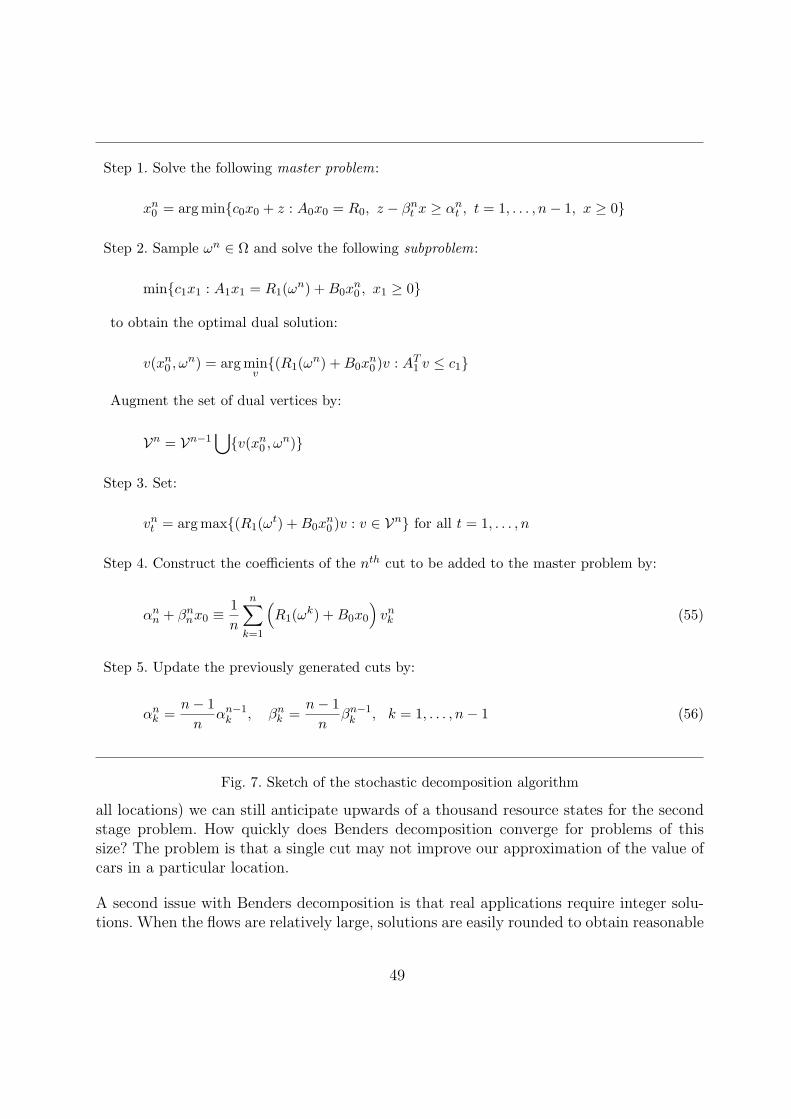
Step 1. Solve the following master problem:

xn0 = arg minc0x0 + z : A0x0 = R0, z − βn

t x ≥ αnt , t = 1, . . . , n− 1, x ≥ 0

Step 2. Sample ωn ∈ Ω and solve the following subproblem:

minc1x1 : A1x1 = R1(ωn) + B0xn0 , x1 ≥ 0

to obtain the optimal dual solution:

v(xn0 , ωn) = arg min

v(R1(ωn) + B0x

n0 )v : AT

1 v ≤ c1

Augment the set of dual vertices by:

Vn = Vn−1⋃v(xn

0 , ωn)

Step 3. Set:

vnt = arg max(R1(ωt) + B0x

n0 )v : v ∈ Vn for all t = 1, . . . , n

Step 4. Construct the coefficients of the nth cut to be added to the master problem by:

αnn + βn

nx0 ≡1n

n∑k=1

(R1(ωk) + B0x0

)vnk (55)

Step 5. Update the previously generated cuts by:

αnk =

n− 1n

αn−1k , βn

k =n− 1

nβn−1

k , k = 1, . . . , n− 1 (56)

Fig. 7. Sketch of the stochastic decomposition algorithm

all locations) we can still anticipate upwards of a thousand resource states for the secondstage problem. How quickly does Benders decomposition converge for problems of thissize? The problem is that a single cut may not improve our approximation of the value ofcars in a particular location.

A second issue with Benders decomposition is that real applications require integer solu-tions. When the flows are relatively large, solutions are easily rounded to obtain reasonable

49

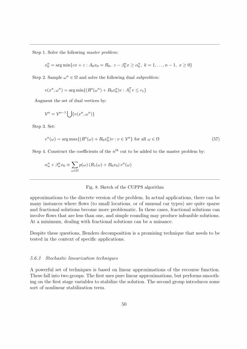
Step 1. Solve the following master problem:

xn0 = arg mincx + z : A0x0 = R0, z − βn

k x ≥ αnk , k = 1, . . . , n− 1, x ≥ 0

Step 2. Sample ωn ∈ Ω and solve the following dual subproblem:

v(xn, ωn) = arg min(Ro(ωn) + B0xn0 )v : AT

1 v ≤ c1

Augment the set of dual vertices by:

Vn = Vn−1⋃v(xn, ωn)

Step 3. Set:

vn(ω) = arg max(Ro(ω) + B0xn0 )v : v ∈ Vn for all ω ∈ Ω (57)

Step 4. Construct the coefficients of the nth cut to be added to the master problem by:

αnn + βn

nx0 ≡∑ω∈Ω

p(ω) (R1(ω) + B0x0) vn(ω)

Fig. 8. Sketch of the CUPPS algorithm

approximations to the discrete version of the problem. In actual applications, there can bemany instances where flows (to small locations, or of unusual car types) are quite sparseand fractional solutions become more problematic. In these cases, fractional solutions caninvolve flows that are less than one, and simple rounding may produce infeasible solutions.At a minimum, dealing with fractional solutions can be a nuisance.

Despite these questions, Benders decomposition is a promising technique that needs to betested in the context of specific applications.

5.6.3 Stochastic linearization techniques

A powerful set of techniques is based on linear approximations of the recourse function.These fall into two groups. The first uses pure linear approximations, but performs smooth-ing on the first stage variables to stabilize the solution. The second group introduces somesort of nonlinear stabilization term.

50

The pure linearization strategy solves sequences of problems of the form:

xn0 = arg min

x0c0x0 + qn−1 ·R1(x0) (58)

To calculate qn, let qn as before be our stochastic gradient obtained as the dual variableof the resource constraint from the second stage using a Monte Carlo realization ωn. Wethen smooth these gradients to obtain:

qn = (1− αn)qn−1 + αnqn (59)

Having obtained the solution xn1 , we then smooth this as well:

xn1 = (1− βn)xn−1

1 + βnxn1 (60)

For both equations (59) and (60), we would normally require the usual conditions onthe stepsizes for stochastic problems, namely that

∑∞n=0 α

n = ∞ and∑∞

n=0(αn)2 < ∞,

although we note in passing that this is not normally satisfied by the stepsize rules usedin practice.

Stochastic linearization techniques are clearly the simplest to use, but are unlikely towork in practice simply because of the lack of stability. Stability is imposed on the so-lution primarily through the use of declining stepsizes, but this is an artificial form ofstability. Furthermore, the smoothing on the first stage variables performed in (60) is aserious practical problem because it completely destroys integrality. Rounding is hard forlarge problems because it can be difficult ensuring conservation of flow in the presence ofsubstitutable resources.

Despite these weaknesses, techniques based on linear approximations are attractive fortransportation applications since they retain the structure of the original problem. If thefirst stage is a network problem, then adding a linear adjustment term retains this property.Linear approximations are also easy to compute and store. We may be able to overcomethe instability of pure linearization techniques by employing any of a variety of nonlin-ear stabilization terms. One notable example is proximal point algorithms, which solvesequences of problems of the form:

xn0 = arg min

x0c0x0 + qn−1 ·R1(x0) + θψ(x0, x

n−10 )

where ψ(x, xn−1) is a distance metric such as ψ(x, xn−1) = ‖x − xn−1‖2. xn is computedusing:

51

xn = (1− βn)xn−1 + βnxn

Note that at the last iteration, the final solution is xn, not xn. xn is used only to stabilizethe solution.

In engineering practice, we can be creative in the construction of the distance metricψ(x, xn−1). If it is separable in x, then we may find ourselves solving a separable, convexoptimization problem. If we are particularly interested in integer solutions, we can con-struct a piecewise linear function defined on discrete values of x (even if xn−1 is fractional).

A second type of nonlinear stabilization strategy is the SHAPE algorithm first presented insection 5.5.2. This is a type of auxiliary function algorithm where we start with an artificialauxiliary function Q0(R), and then update it using stochastic gradients as demonstratedin equation (31). An attractive feature of this algorithm is that the auxiliary functioncan (and should) be chosen to retain the structure of the first stage problem as muchas possible. For our car distribution problem (and similar applications), piecewise linear,separable approximations are particularly attractive.

5.6.4 Nonlinear functional approximations

Our last class of strategies tries to explicitly approximate the recourse function, withoutany guarantee of convergence to the exact function. We do not include algorithms suchas the one-sided SHAPE algorithm (equation (31)) in this group because there is noexplicit attempt to approximate the recourse function. We also do not include Bendersdecomposition simply because we feel that this strategy is in a class by itself. But we doinclude both the two-sided SHAPE algorithm (equation (32)) and the structured adaptivefunctional estimators.

We first introduced these algorithms in the context of a recourse function Q(R) whichcould be written as a separable function of the resource vector R. Now consider whatwould happen if we apply the exact same algorithms to a nonseparable problem. We stillproduce a separable approximation of Q, and we still solve sequences of networks that areidentical to figure 5. The important difference is that we are solving sequences of sepa-rable approximations of otherwise nonseparable functions. For continuously differentiableproblems, this can be an optimal strategy (in the limit). For nondifferentiable problems(as we are considering) the result is an algorithm that is very near optimal with a muchfaster rate of convergence than has been achieved using Benders decomposition.

52

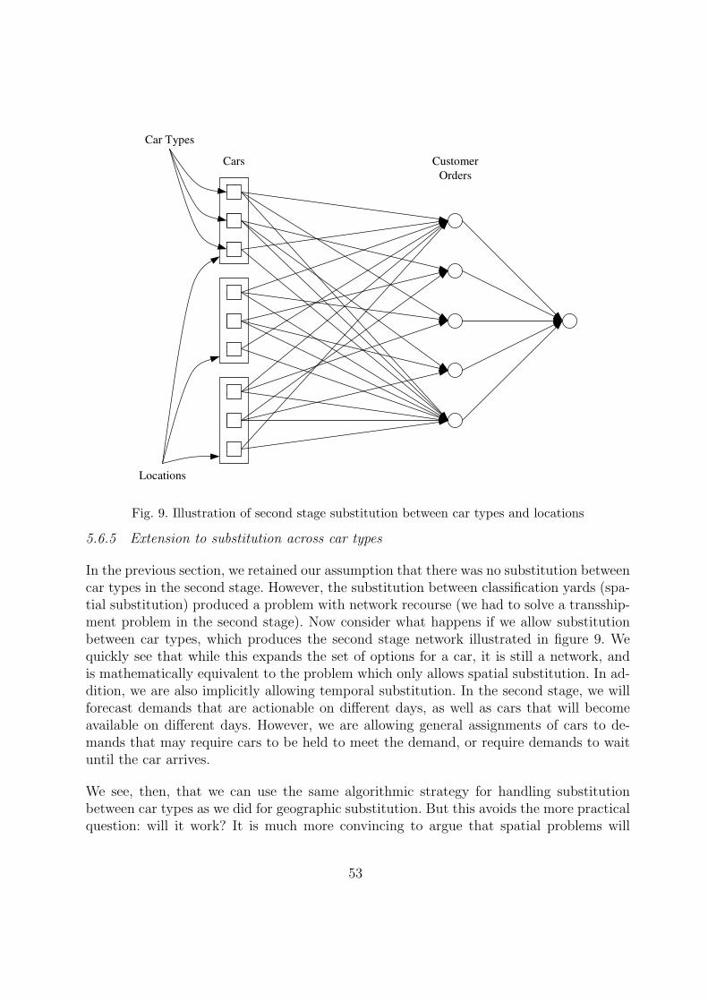
Fig. 9. Illustration of second stage substitution between car types and locations

5.6.5 Extension to substitution across car types

In the previous section, we retained our assumption that there was no substitution betweencar types in the second stage. However, the substitution between classification yards (spa-tial substitution) produced a problem with network recourse (we had to solve a transship-ment problem in the second stage). Now consider what happens if we allow substitutionbetween car types, which produces the second stage network illustrated in figure 9. Wequickly see that while this expands the set of options for a car, it is still a network, andis mathematically equivalent to the problem which only allows spatial substitution. In ad-dition, we are also implicitly allowing temporal substitution. In the second stage, we willforecast demands that are actionable on different days, as well as cars that will becomeavailable on different days. However, we are allowing general assignments of cars to de-mands that may require cars to be held to meet the demand, or require demands to waituntil the car arrives.

We see, then, that we can use the same algorithmic strategy for handling substitutionbetween car types as we did for geographic substitution. But this avoids the more practicalquestion: will it work? It is much more convincing to argue that spatial problems will

53

produce approximately separable recourse functions than would arise in the case withother forms of substitution. For example, it is quite likely that the cost of substitutingother box cars in the same car group is quite small. In fact, this is the reason that arailroad might reasonably ignore car subgroups and just model car groups.

For two-stage problems, there is a strong reason to believe that separable approximationswill work well, even when the recourse function is not even approximately separable. Thelogic behind this argument is that for n sufficiently large, Qn will stabilize, and therefore sowill xn

0 . As xn0 (approximately) approaches a limit point, Rn

1 (xn0 ) will approach a limit point,

allowing us to produce an accurate (but not perfect) piecewise linear approximation Qnj (Rj)

of the jth dimension of Q(R), at the point R = Rn1 (xn

0 ). Thus, a separable approximationonly needs to be a good local approximation to provide good results.

5.6.6 Summary

The choice of the best algorithm for two-stage resource allocation problems remains anopen question. Two-stage problems are an important foundational problem, but in trans-portation applications, the usual goal is to solve multistage problems. However, it is im-portant to study the performance of an algorithm in a two-stage setting first, and it isdifficult to believe that an algorithm that does not work well for two-stage problems wouldturn out to work well in a multistage application. But the converse may not be true; analgorithm that does work well for a two-stage problem may not work well in a multistagesetting. It is possible for an algorithm (such as the separable, nonlinear functional approx-imations) to exploit the limiting behavior of the first stage decisions, a property that welose immediately in the context of multistage problems.

Our belief is that while scenario methods are unlikely to prove attractive in practice, theother three major classes of techniques (Benders decomposition, stochastic linearizationwith nonlinear stabilization strategies, or nonlinear functional approximations) all deserveserious study. We believe that nonlinear functional approximations are going to work thebest for two-stage problems because a) they attempt to explicitly approximate the re-course function and b) they exploit the structure of problems that arise in transportation.However, we have not yet addressed some of the more difficult dimensions of transporta-tion applications (some of which are touched on below). Nonlinear approximations canwork the best in laboratory experiments, but are much more difficult to use than linearapproximations. Pure linear approximations are too unstable, but linear approximationswith nonlinear stabilization terms (proximal point algorithms or auxiliary functions) mayoffer an attractive alternative. All of these approximations are separable, and it is simplynot clear how well these will work in multistage applications.

54

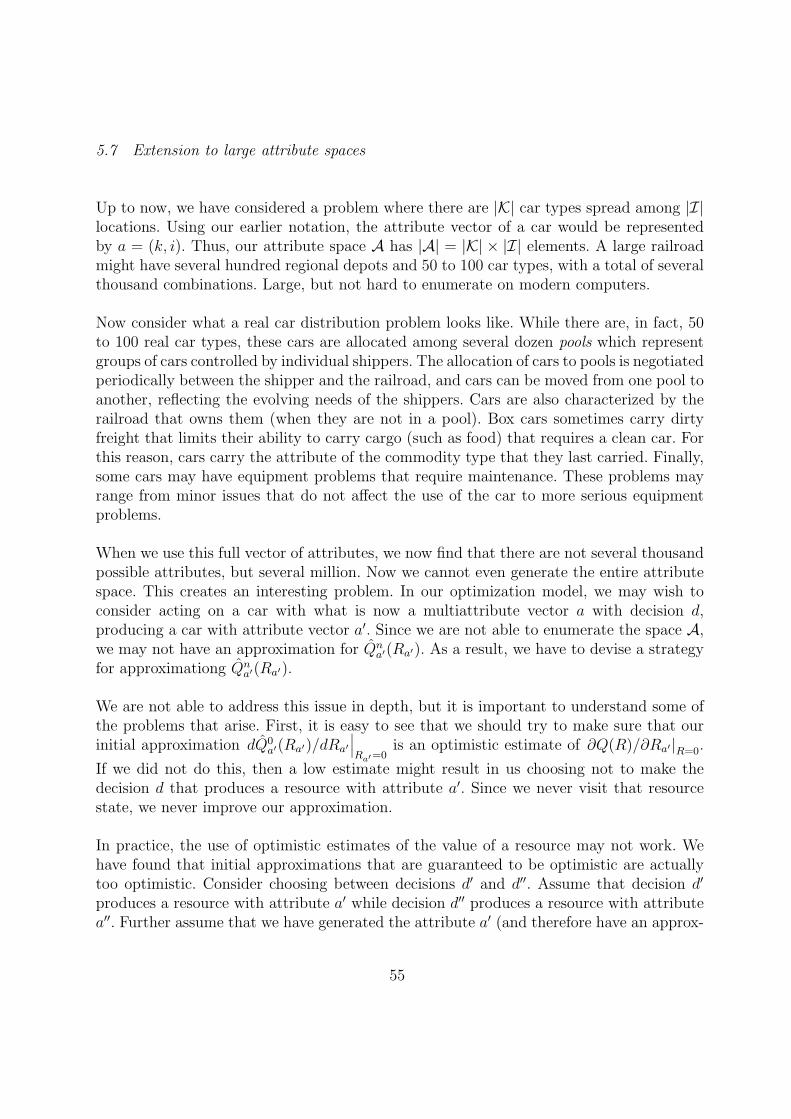
5.7 Extension to large attribute spaces

Up to now, we have considered a problem where there are |K| car types spread among |I|locations. Using our earlier notation, the attribute vector of a car would be representedby a = (k, i). Thus, our attribute space A has |A| = |K| × |I| elements. A large railroadmight have several hundred regional depots and 50 to 100 car types, with a total of severalthousand combinations. Large, but not hard to enumerate on modern computers.

Now consider what a real car distribution problem looks like. While there are, in fact, 50to 100 real car types, these cars are allocated among several dozen pools which representgroups of cars controlled by individual shippers. The allocation of cars to pools is negotiatedperiodically between the shipper and the railroad, and cars can be moved from one pool toanother, reflecting the evolving needs of the shippers. Cars are also characterized by therailroad that owns them (when they are not in a pool). Box cars sometimes carry dirtyfreight that limits their ability to carry cargo (such as food) that requires a clean car. Forthis reason, cars carry the attribute of the commodity type that they last carried. Finally,some cars may have equipment problems that require maintenance. These problems mayrange from minor issues that do not affect the use of the car to more serious equipmentproblems.

When we use this full vector of attributes, we now find that there are not several thousandpossible attributes, but several million. Now we cannot even generate the entire attributespace. This creates an interesting problem. In our optimization model, we may wish toconsider acting on a car with what is now a multiattribute vector a with decision d,producing a car with attribute vector a′. Since we are not able to enumerate the space A,we may not have an approximation for Qn

a′(Ra′). As a result, we have to devise a strategyfor approximationg Qn

a′(Ra′).

We are not able to address this issue in depth, but it is important to understand some ofthe problems that arise. First, it is easy to see that we should try to make sure that ourinitial approximation dQ0

a′(Ra′)/dRa′

∣∣∣Ra′=0

is an optimistic estimate of ∂Q(R)/∂Ra′|R=0.

If we did not do this, then a low estimate might result in us choosing not to make thedecision d that produces a resource with attribute a′. Since we never visit that resourcestate, we never improve our approximation.

In practice, the use of optimistic estimates of the value of a resource may not work. Wehave found that initial approximations that are guaranteed to be optimistic are actuallytoo optimistic. Consider choosing between decisions d′ and d′′. Assume that decision d′

produces a resource with attribute a′ while decision d′′ produces a resource with attributea′′. Further assume that we have generated the attribute a′ (and therefore have an approx-

55

imation Qna′(Ra′)), but we have never generated the attribute a′′. If we use an optimistic

approximation for Qna′′(Ra′′), then we would choose d′′ just because we have never tried

it before. The result is the steady exploration of every possible decision, and a virtualenumeration of the attribute space A.

A more practical approach is to assume that we have access to an aggregation functionG(a) 7→ a where a ∈ A is an aggregation of the original attribute space. We assume thatA is not too large and can be enumerated. We further assume that Qn

a(Ra) is a “good”approximation of Qn

a(Ra) when G(a) = a. We then make sure that we repeatedly samplegradients and update Qn

a(Ra) for all a ∈ A.

We are not aware of any formal convergence theory for this approach (or for any otheralgorithm for this problem class). But real problems in transportation are characterized bya much richer vector of attributes than is normally considered by the academic community.

6 Multistage resource allocation problems

We now turn to the challenge of solving multistage problems. In multistage problems,we have to capture the sequential decision-making process as information (and decisions)evolve over time. For transportation problems, we encounter the reusability of resources;once a vehicle moves a load, it is available to be used again.

We could motivate our multistage problem using our rail car distribution example, but itis useful to bring other applications into the picture. Examples include:

1) Fleet management for truckload trucking - In truckload trucking, a truck moves an entireload of freight from origin to destination. Uncertainty plays a major role in the long haultruckload market, where loads can take between one and four days to deliver. Customerssometimes request trucks the same day the order is made, but more often call in oneor two days in advance. In sharp contrast with the rail industry, the truckload carrierdoes not have to accept every load, and this is one of the major challenges. Emergingelectronic market places, where loads are posted on web sites, open the possibility oftaking loads that do not have to move for several days. This is a classic problem ofdecision-making under uncertainty.

2) Driver management for long-haul less-than-truckload motor carriers - LTL carriers facethe problem of timing the movement of loads over the network, requiring the carefulmanagement of drivers.

3) Management of jets in the fractional ownership industry - In this business, high networth individuals and business executives will own a fraction of a jet. This gives them

56

access to the entire fleet of jets. They may call the company with as little as eight hoursnotice and request that a jet move them from a local airport to any other airport. Afterthe move, the fleet operator will move the jet to another location.

4) Routing and scheduling transport aircraft for the air mobility command - The AMCworks like a large trucking company, moving freight for the military using large transportaircraft. They are typically used in support of emergency situations where requests forfreight movement arise dynamically.

Compared to our rail car distribution problem, these applications are characterized byrelatively shorter travel times and less flexibility to satisfy customer orders at times otherthan when they were requested.

Multistage problems are, of course, much harder than two-stage problems, but we are goingto approach them by building on the tools we have already introduced. Our strategy forsolving multistage problems is to solve them as sequences of two-stage problems. Studentsof dynamic programming will see strong similarities in our modeling approach. But mul-tistage problems do introduce a fresh set of modeling and algorithmic issues that simplydo not arise in two-stage problems.

We start in section 6.1 with a formulation of the problem. Then, Section 6.2 outlines thegeneral algorithmic strategy. Section 6.3 describes the implementation in the context ofsingle commodity flow problems. Section 6.4 outlines the challenges that arise when wesolve multicommodity problems in a multistage setting. Finally, section 6.5 describes thecomplications that are introduced when we model the property that it takes more thanone time period to go from one location to another.

6.1 Formulation

We present the basic multistage problem with somewhat more generality than we haveused previously. We first define the exogenous information arriving to our system:

Rt = Vector of new arrivals in period t, where Rt = (Rot , R

ct).

ξt = Complete vector of new information arriving in period t, including both Rt as wellas other information about system parameters (travel times, costs, and parametersgoverning the physics of the problem).

For our purposes, we are only interested in the resource state Rt, and the only informationprocess we are modeling at the moment is the arrival of new resources, Rt. Using thisnotation, our history of states, information and decisions (given earlier in equation (7))would look like:

57

ht = R+0 , x0, R0, R1, R

+1 , x1, R1, R2, R

+2 , x2, R2, . . . , Rt, R

+t , xt, Rt, . . . (61)

There are three perspectives of the state of our system:

Rt = Vector of resources available in period t after decisions xt have been made.Kt = What is known at time t after the new information ξt has been incorporated. Kt

includes Rt plus what we know about parameters that govern the dynamics of thesystem.

It = Set of information available at time t for making a decision. It includes Kt, but itmight also include forecasts of future activities (activities which are not “known” now,but are the result of a forecasting exercise).

Our process is controlled by the decisions we make:

xt = Decisions which are made after new information in period t has become known.Xπ

t (It) = The decision function of policy π.

Our decisions are chosen to maximize the expected total contribution over a planninghorizon. Our contribution function is expressed as:

ct(xt, Kt) = The contribution generated in period t given decision xt, and what is known, Kt.

When resources are allocated in time t, they have to satisfy flow conservation equations ofthe form:

∑d∈D

xtad =Rt−1,at + Rt,at

where we assume that we can only act on resources that are actionable now (Rtt). Thephysical dynamics of the system are given by:

Rt,a′t′ =Rt−1,a′t′ +∑a∈A

∑d∈Da

δt′,a′(t, a, d)xtad ∀a′ ∈ A, t′ ≥ t+ 1. (62)

It is often useful to express flow conservation and system dynamics in matrix form, whichwe do using:

Atxt =Rt−1 + Rt (63)

Rt −Btxt = 0 (64)

58

For reasons that are made clear in section 6.2, we have written our equations directlyin terms of the incomplete resource vector Rt. The complete resource vector is simplyR+

t = Rt−1 + Rt.

The informational dynamics can be written generally as:

Kt+1 =UK(Kt, ξt+1) (65)

which is how we would represent the process of updating demand forecasting equations,parameter estimation equations, and the storage of other types of information.

The basic statement of the multistage problem is now given by:

maxπ∈Π

E

∑t∈T

ct(Xπ(It), Kt)

subject to flow conservation (equation (63)), resource dynamics (equation (64)) and infor-mational dynamics (equation (65)). There may also be upper bounds on flows representingphysical constraints.

The challenge, now, is choosing a function Xπ(It). Popular choices include myopic policies(It = Kt), or rolling horizon procedures, where It = (Kt, Ωt) where Ωt represents a forecastof future events made with the information known at time t. If |Ωt| = 1 then we are usinga point estimate of the future and we obtain classical deterministic methods for handlingthe future. In the next section, we discuss how adaptive dynamic programming methodscan be used.

6.2 Our algorithmic strategy

Our strategy for solving multistage problems is based on techniques from approximatedynamic programming. Since this approach is not familiar to the stochastic programmingcommunity, some background presentation is useful. Recall from section 6.1 (and in par-ticular equation (61) that we can measure the state of our system before or after we makea decision. It is common in the dynamic programming and control community to writethe optimality equations using the state before we make a decision, producing optimalityequations of the form:

Q+t (R+

t ) = arg maxxt

ct(Xπ(It), R

+t ) + E

Q+

t+1(R+t+1)|R+

t

(66)

59

Classical dynamic programming techniques are computationally intractable for this prob-lem class. Solving equation (66) using classical discrete dynamic programming techniquesencounters three “curses of dimensionality”: the state space, the outcome space and theaction space. Each of these variables are vectors (and potentially vectors of high dimen-sionality). Computing the value functions using a backward recursion requires computingequation (66) for each possible value of the state variable. Computing the expectationrequires summing over all the outcomes in the outcome space. Finally, since the expectedvalue function may not have any special structure, solving the optimization problem re-quires evaluating all possible values of the decision vector xt.

We overcome this problem using the following strategy. First, recognizing that we do notknowQ+

t+1, we replace it with an appropriate approximation that for the moment we denote

by Q+t+1(R

+t+1). Next, we recognize that we cannot compute the expectation in (66). The

common strategy is to replace the expectation with an approximation based on a sampletaking from the outcome space:

Q+t (R+

t ) = arg maxxt

ct(Xπ(It), R

+t ) +

∑ω∈Ω

p(ω)Q+t+1(R

+t+1(ω)) (67)

Equation (67) can be exceptionally difficult to solve for the types of high dimensional, dis-crete resource allocation problems that arise in transportation. It is particularly inelegantwhen we realize that it is often the case that the myopic problem (maximizing ctxt) is apure network, which means the introduction of the approximate value function is makinga trivial integer program quite difficult (the LP relaxation is not a good approximation).

Equation (67) is quite easy to solve if we use a linear approximation for Qt+1. In this case:

Q+t+1(R

+t+1) = q+

t+1 ·R+t+1

= q+t+1 · (Rt + Atxt + Rt+1) (68)

Taking conditional expectations of both sides of (68) gives:

EQ+t+1(R

+t+1)|R+

t =Eq+t+1 · (Rt + Atxt + Rt+1)|R+

t = q+

t+1Rt + q+t+1Atxt + Eq+

t+1Rt+1|R+t (69)

The only term on the right hand side of (69) involving the expectation is not a function ofxt, so it is only a constant term and can be dropped. The resulting optimization problem isidentical to the original myopic optimization problem with a linear adjustment term whichwould never destroy any nice structural properties of the original problem (for example,network structure).

60

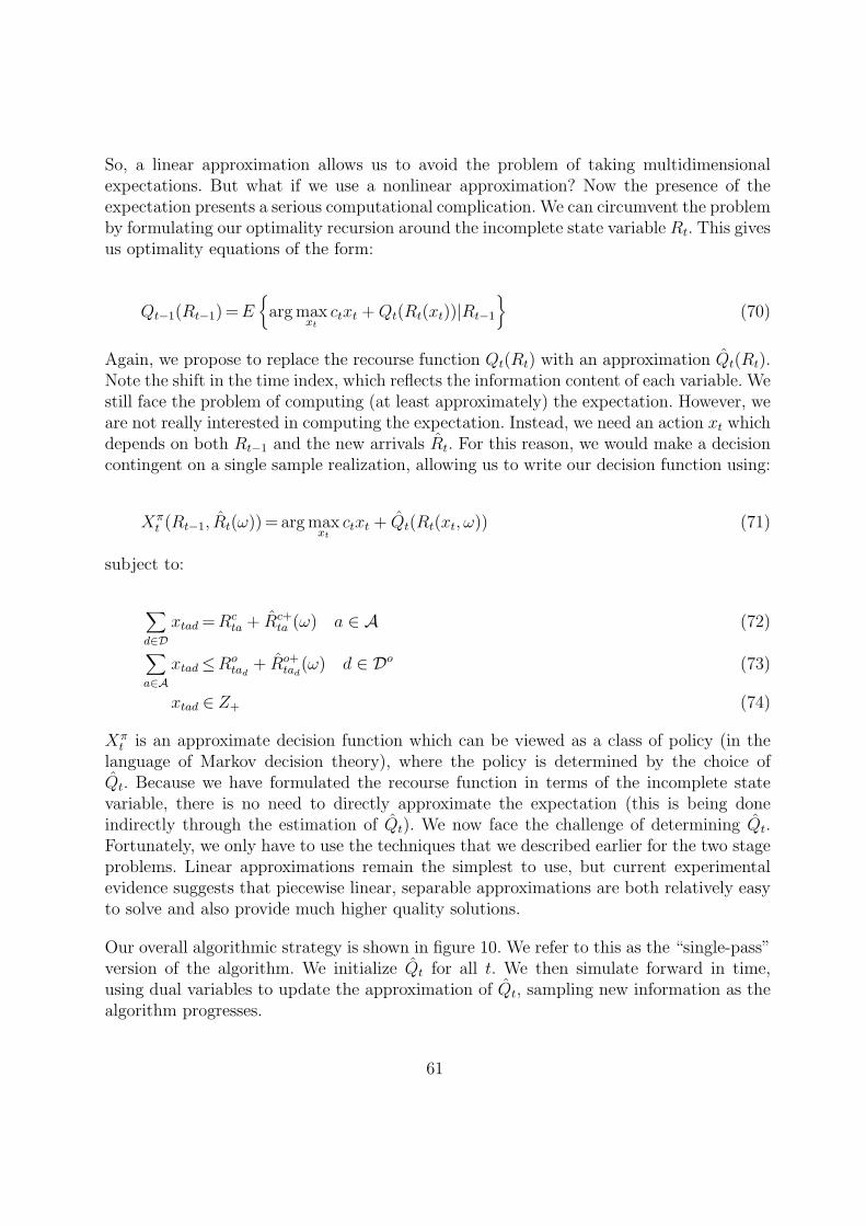
So, a linear approximation allows us to avoid the problem of taking multidimensionalexpectations. But what if we use a nonlinear approximation? Now the presence of theexpectation presents a serious computational complication. We can circumvent the problemby formulating our optimality recursion around the incomplete state variable Rt. This givesus optimality equations of the form:

Qt−1(Rt−1) =Earg max

xtctxt +Qt(Rt(xt))|Rt−1

(70)

Again, we propose to replace the recourse function Qt(Rt) with an approximation Qt(Rt).Note the shift in the time index, which reflects the information content of each variable. Westill face the problem of computing (at least approximately) the expectation. However, weare not really interested in computing the expectation. Instead, we need an action xt whichdepends on both Rt−1 and the new arrivals Rt. For this reason, we would make a decisioncontingent on a single sample realization, allowing us to write our decision function using:

Xπt (Rt−1, Rt(ω)) = arg max

xtctxt + Qt(Rt(xt, ω)) (71)

subject to:

∑d∈D

xtad =Rcta + Rc+

ta (ω) a ∈ A (72)

∑a∈A

xtad≤Rotad

+ Ro+tad

(ω) d ∈ Do (73)

xtad ∈ Z+ (74)

Xπt is an approximate decision function which can be viewed as a class of policy (in the

language of Markov decision theory), where the policy is determined by the choice ofQt. Because we have formulated the recourse function in terms of the incomplete statevariable, there is no need to directly approximate the expectation (this is being doneindirectly through the estimation of Qt). We now face the challenge of determining Qt.Fortunately, we only have to use the techniques that we described earlier for the two stageproblems. Linear approximations remain the simplest to use, but current experimentalevidence suggests that piecewise linear, separable approximations are both relatively easyto solve and also provide much higher quality solutions.

Our overall algorithmic strategy is shown in figure 10. We refer to this as the “single-pass”version of the algorithm. We initialize Qt for all t. We then simulate forward in time,using dual variables to update the approximation of Qt, sampling new information as thealgorithm progresses.

61

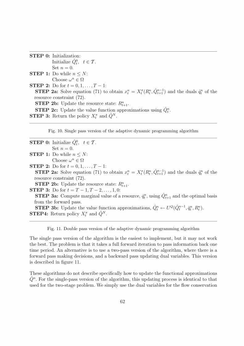
STEP 0: Initialization:Initialize Q0

t , t ∈ T .Set n = 0.

STEP 1: Do while n ≤ N :Choose ωn ∈ Ω

STEP 2: Do for t = 0, 1, . . . , T − 1:STEP 2a: Solve equation (71) to obtain xn

t = Xπt (Rn

t , Qn−1t+1 ) and the duals qn

t of theresource constraint (72).STEP 2b: Update the resource state: Rn

t+1.

STEP 2c: Update the value function approximations using Qnt .

STEP 3: Return the policy Xπt and QN .

Fig. 10. Single pass version of the adaptive dynamic programming algorithm

STEP 0: Initialize Q0t , t ∈ T .

Set n = 0.STEP 1: Do while n ≤ N :

Choose ωn ∈ ΩSTEP 2: Do for t = 0, 1, . . . , T − 1:

STEP 2a: Solve equation (71) to obtain xnt = Xπ

t (Rnt , Q

n−1t+1 ) and the duals qn

t of theresource constraint (72).STEP 2b: Update the resource state: Rn

t+1.STEP 3: Do for t = T − 1, T − 2, . . . , 1, 0:

STEP 3a: Compute marginal value of a resource, qnt , using Qn

t+1 and the optimal basisfrom the forward pass.STEP 3b: Update the value function approximations, Qn

t ← UQ(Qn−1t , qn

t , Rnt ).

STEP4: Return policy Xπt and QN .

Fig. 11. Double pass version of the adaptive dynamic programming algorithm

The single pass version of the algorithm is the easiest to implement, but it may not workthe best. The problem is that it takes a full forward iteration to pass information back onetime period. An alternative is to use a two-pass version of the algorithm, where there is aforward pass making decisions, and a backward pass updating dual variables. This versionis described in figure 11.

These algorithms do not describe specifically how to update the functional approximationsQn. For the single-pass version of the algorithm, this updating process is identical to thatused for the two-stage problem. We simply use the dual variables for the flow conservation

62

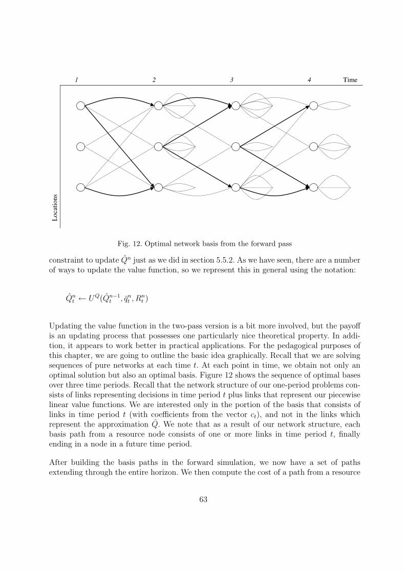
Fig. 12. Optimal network basis from the forward pass

constraint to update Qn just as we did in section 5.5.2. As we have seen, there are a numberof ways to update the value function, so we represent this in general using the notation:

Qnt ← UQ(Qn−1

t , qnt , R

nt )

Updating the value function in the two-pass version is a bit more involved, but the payoffis an updating process that possesses one particularly nice theoretical property. In addi-tion, it appears to work better in practical applications. For the pedagogical purposes ofthis chapter, we are going to outline the basic idea graphically. Recall that we are solvingsequences of pure networks at each time t. At each point in time, we obtain not only anoptimal solution but also an optimal basis. Figure 12 shows the sequence of optimal basesover three time periods. Recall that the network structure of our one-period problems con-sists of links representing decisions in time period t plus links that represent our piecewiselinear value functions. We are interested only in the portion of the basis that consists oflinks in time period t (with coefficients from the vector ct), and not in the links whichrepresent the approximation Q. We note that as a result of our network structure, eachbasis path from a resource node consists of one or more links in time period t, finallyending in a node in a future time period.

After building the basis paths in the forward simulation, we now have a set of pathsextending through the entire horizon. We then compute the cost of a path from a resource

63

node t for attribute vector a until the end of the horizon. Let qnta be the cost of the path

from resource node a at time t until the end of the horizon along this basis path. Thesepath costs have a very nice property. Let:

F πt (Rt, ω

n) =T∑

t′=t

ctXπt (It(ω

n)) (75)

be the costs of a policy π (determined by the functional approximation Qn) for outcomeωn in iteration n, starting in time period t. Then we have:

Theorem 2 Let qnt = (qn

ta)a∈A be the vector of path costs from time t to the end of the hori-zon, given outcome ωn and functional approximations Qn

t t∈T computed from a backwardpass. Then qt satisfies:

F πt (Rt, ω

n)− F πt (R′

t, ωn) ≤ qn

t · (Rt −R′t)

Furthermore, if the basis paths in each period t are flow augmenting paths into the super-sink, then qn

t is a right gradient of F πt (Rt, ω

n).

This is a very nice result. These paths are not too hard to compute and provide accurateestimates of the future value of a resource. It turns out that the ability to compute rightderivatives is very important. If we just use the dual variables, we overestimate the valueof a resource in the future, producing unwanted empty moves.

With our ability to compute valid stochastic gradients of the cost function, we are readyto apply all the tricks we learned for two-stage problems for computing the approximatevalue functions, Qn

t . The forward pass/backward pass logic is easy to execute and compu-tationally tractable. The Monte Carlo sampling logic avoids problems with expectations.This almost looks too good to be true.

Multistage problems, however, have a few more surprises for us. We begin by discussingthe problem of computing expectations, even when we use approximations of the recoursefunction. We next focus on the issue of problem structure. Keep in mind that transporta-tion problems can be very large, and we are still interested in integer solutions. The firstchallenge that arises in multistage problems is that resources are reusable (box cars do notsimply vanish after we use them). This introduces structural problems that did not occurwith two-stage problems, which we review in the context of both single and multicom-modity flow problems. We then briefly discuss one of the more annoying, but unavoidable,features of transportation problems: multiperiod travel times.

64

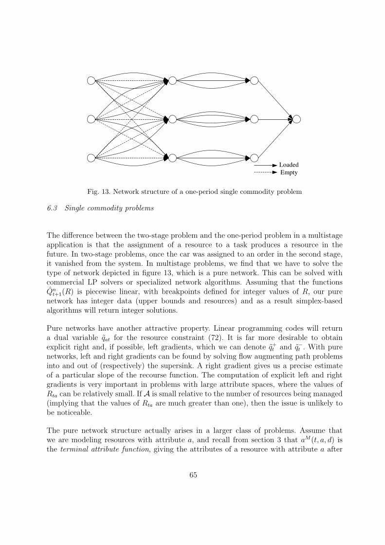
Fig. 13. Network structure of a one-period single commodity problem

6.3 Single commodity problems

The difference between the two-stage problem and the one-period problem in a multistageapplication is that the assignment of a resource to a task produces a resource in thefuture. In two-stage problems, once the car was assigned to an order in the second stage,it vanished from the system. In multistage problems, we find that we have to solve thetype of network depicted in figure 13, which is a pure network. This can be solved withcommercial LP solvers or specialized network algorithms. Assuming that the functionsQn

t+1(R) is piecewise linear, with breakpoints defined for integer values of R, our purenetwork has integer data (upper bounds and resources) and as a result simplex-basedalgorithms will return integer solutions.

Pure networks have another attractive property. Linear programming codes will returna dual variable qat for the resource constraint (72). It is far more desirable to obtainexplicit right and, if possible, left gradients, which we can denote q+

t and q−t . With purenetworks, left and right gradients can be found by solving flow augmenting path problemsinto and out of (respectively) the supersink. A right gradient gives us a precise estimateof a particular slope of the recourse function. The computation of explicit left and rightgradients is very important in problems with large attribute spaces, where the values ofRta can be relatively small. If A is small relative to the number of resources being managed(implying that the values of Rta are much greater than one), then the issue is unlikely tobe noticeable.

The pure network structure actually arises in a larger class of problems. Assume thatwe are modeling resources with attribute a, and recall from section 3 that aM(t, a, d) isthe terminal attribute function, giving the attributes of a resource with attribute a after

65

decision d has been applied to it. Now define:

Definition 3 A resource allocation problem has the Markov property if aM(t, a, d) =aM(t, a′, d), ∀a, a′ ∈ A.

The Markov property for resource allocation problems implies that the attributes of aresource after it has been acted on is purely a function of the decision. Classical singlecommodity flow problems exhibit this property because a truck in location i which is thenassigned to move a load from i to j, is now a truck at location j. If all the trucks are thesame, then the attribute of the truck (its location) is purely a function of the attribute ofthe decision which was to move a load to j. If there were different types of trucks that couldserve the load (a multicommodity problem), then the attribute of the truck after movingthe load continues to have the attribute of the truck before the load (a characteristic thathas nothing to do with the decision).

It is apparent that classical multicommodity problems which allow substitution of differentcommodity types for the same task will never have the Markov property, but multiattributeproblems (where the attribute vector a consists purely of dynamic attributes), can possessthis property. Consider a chemical trailer that can move basic argon gas or purified argongas. Only “clean” trailers can move purified argon gas. A clean trailer can move basicgas, but then it is no longer clean. There is no substitution for purified argon gas, andany truck moving basic argon gas is no longer clean (although it can be put through acleansing process). Thus, the attributes of the truck after a trip are determined completelyby the characteristics of the trip.

6.4 Multicommodity problems

When we encountered single commodity problems, we found that the single period prob-lems were pure networks if the approximation of the recourse function were linear, orpiecewise linear, separable. Now we consider what happens when we try to solve mul-ticommodity problems. Recall that we let I be a set of locations and K be the set ofcommodities. We follow the standard notation of multicommodity flow problems and letRk

ti be the number of resources of type k in location i, and let xktdi be the number of

resources of type k in location i that we act on with decision d at time t.

Section 6.4.1 shows that multistage, multicommodity problems are especially easy to solveif we use linear approximations for the recourse function. The only issue is that the solutionquality is not that high. Then, section 6.4.2 outlines the complications that arise when weuse piecewise linear, separable approximations.

66

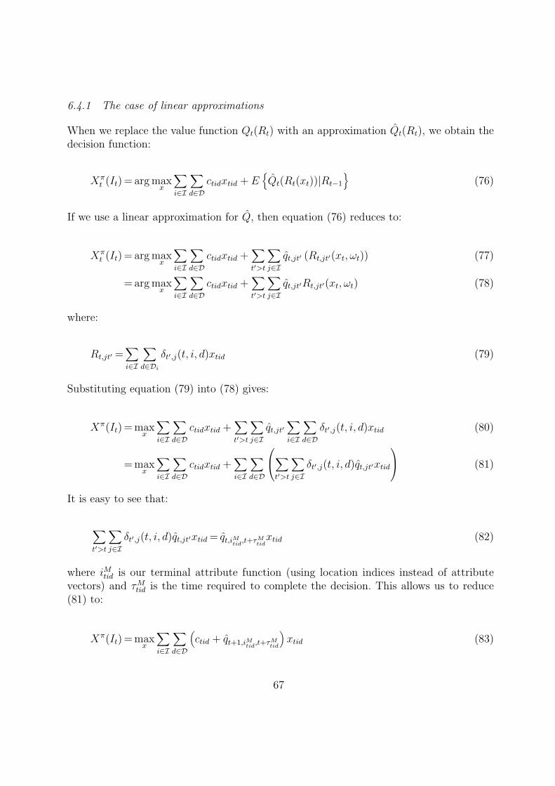
6.4.1 The case of linear approximations

When we replace the value function Qt(Rt) with an approximation Qt(Rt), we obtain thedecision function:

Xπt (It) = arg max

x

∑i∈I

∑d∈D

ctidxtid + EQt(Rt(xt))|Rt−1

(76)

If we use a linear approximation for Q, then equation (76) reduces to:

Xπt (It) = arg max

x

∑i∈I

∑d∈D

ctidxtid +∑t′>t

∑j∈I

qt,jt′ (Rt,jt′(xt, ωt)) (77)

= arg maxx

∑i∈I

∑d∈D

ctidxtid +∑t′>t

∑j∈I

qt,jt′Rt,jt′(xt, ωt) (78)

where:

Rt,jt′ =∑i∈I

∑d∈Di

δt′,j(t, i, d)xtid (79)

Substituting equation (79) into (78) gives:

Xπ(It) = maxx

∑i∈I

∑d∈D

ctidxtid +∑t′>t

∑j∈I

qt,jt′∑i∈I

∑d∈D

δt′,j(t, i, d)xtid (80)

= maxx

∑i∈I

∑d∈D

ctidxtid +∑i∈I

∑d∈D

∑t′>t

∑j∈I

δt′,j(t, i, d)qt,jt′xtid

(81)

It is easy to see that:

∑t′>t

∑j∈I

δt′,j(t, i, d)qt,jt′xtid = qt,iMtid

,t+τMtidxtid (82)

where iMtid is our terminal attribute function (using location indices instead of attributevectors) and τM

tid is the time required to complete the decision. This allows us to reduce(81) to:

Xπ(It) = maxx

∑i∈I

∑d∈D

(ctid + qt+1,iM

tid,t+τM

tid

)xtid (83)

67

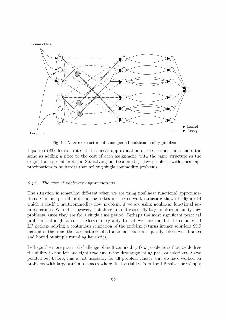
Fig. 14. Network structure of a one-period multicommodity problem

Equation (83) demonstrates that a linear approximation of the recourse function is thesame as adding a price to the cost of each assignment, with the same structure as theoriginal one-period problem. So, solving multicommodity flow problems with linear ap-proximations is no harder than solving single commodity problems.

6.4.2 The case of nonlinear approximations

The situation is somewhat different when we are using nonlinear functional approxima-tions. Our one-period problem now takes on the network structure shown in figure 14which is itself a multicommodity flow problem, if we are using nonlinear functional ap-proximations. We note, however, that these are not especially large multicommodity flowproblems, since they are for a single time period. Perhaps the most significant practicalproblem that might arise is the loss of integrality. In fact, we have found that a commercialLP package solving a continuous relaxation of the problem returns integer solutions 99.9percent of the time (the rare instance of a fractional solution is quickly solved with branchand bound or simple rounding heuristics).

Perhaps the more practical challenge of multicommodity flow problems is that we do losethe ability to find left and right gradients using flow augmenting path calculations. As wepointed out before, this is not necessary for all problem classes, but we have worked onproblems with large attribute spaces where dual variables from the LP solver are simply

68

not good enough. In this case, we are resorting to performing numerical derivatives (in-crementing the right hand side and solving the problem again). Since the optimal basis isoften optimal for the perturbed problem, this procedure can be quite fast.

6.5 The problem of travel times

One of the most annoying characteristics of transportation is the property that it takestime to complete a decision. Using the vocabulary of discrete time models, we refer tothese problems as having “multiperiod” travel times. More generally, we would refer tothese as “multiperiod transfer times,” since there are many activities in transportationthat do not actually involve moving from one location to another (drivers have to go onrest, trailers have to be cleaned, locomotives have to be maintained). But, the concept oftraveling between locations is easy to visualize.

The implication of multiperiod travel times is that after acting on a resource at time t,the resource is committed to an activity in time period t+ 1 and we cannot act on it. Atthe same time, we cannot ignore it, because it will eventually complete its movement, andwe have to take this into account when we make decisions in time period t + 1. Figure15 illustrates the issue in the context of fleet management. Assume that we will needcontainers at location c at time t = 6, and we can move them there from either a, whichis five time periods away, or from d, which is only two time periods away. Because a isfarther away, we will first look at the problem of the shortage of containers at c for timet = 6 at time t = 1. At this point, we would not have considered moving containers fromlocation d, since this decision would not be made until t = 4. Seeing the shortage, wemight move containers the longer distance from a to c, rather than waiting until timet = 4 and moving them from the closer location at d.

The modeling of multiperiod travel times is the same as the modeling of lagged informationprocesses. Earlier in the chapter, we introduced the notation Rtt′ which gives the vector ofresources that we know about at time t which become actionable at time t′. The differencebetween t′ and t is the information lag. Lags can arise when customers call in orders inadvance. In the case of our rail car distribution problem, it can arise when a shipper tellsthe carrier that a freight car will become empty in three days. Information lags also arisewhenever the travel time from one location to another is more than one time period.

The problem of multiperiod travel times is unique to multistage stochastic models, andfurthermore it is unique to the usage of nonlinear functional approximations. With anonlinear function, location a “sees” the steeper part of the slope of the function at c,since we have not yet made the decision to move cars from d. The result is somethingthat we call the “long haul bias,” which arises in any application where resources can be

69

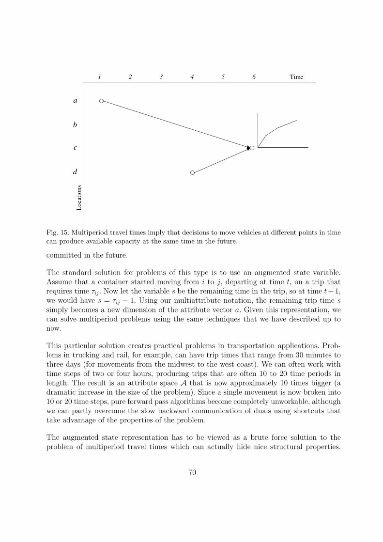
Fig. 15. Multiperiod travel times imply that decisions to move vehicles at different points in timecan produce available capacity at the same time in the future.

committed in the future.

The standard solution for problems of this type is to use an augmented state variable.Assume that a container started moving from i to j, departing at time t, on a trip thatrequires time τij. Now let the variable s be the remaining time in the trip, so at time t+1,we would have s = τij − 1. Using our multiattribute notation, the remaining trip time ssimply becomes a new dimension of the attribute vector a. Given this representation, wecan solve multiperiod problems using the same techniques that we have described up tonow.

This particular solution creates practical problems in transportation applications. Prob-lems in trucking and rail, for example, can have trip times that range from 30 minutes tothree days (for movements from the midwest to the west coast). We can often work withtime steps of two or four hours, producing trips that are often 10 to 20 time periods inlength. The result is an attribute space A that is now approximately 10 times bigger (adramatic increase in the size of the problem). Since a single movement is now broken into10 or 20 time steps, pure forward pass algorithms become completely unworkable, althoughwe can partly overcome the slow backward communication of duals using shortcuts thattake advantage of the properties of the problem.

The augmented state representation has to be viewed as a brute force solution to theproblem of multiperiod travel times which can actually hide nice structural properties.

70

For example, it is not readily apparent using this representation that the problem ofmultiperiod travel times vanishes when we use linear functional approximations. WhenQC,t+6 is a linear function, both locations a and d “see” the same slope. If they both sendcontainers in response to an attractive slope, then the sample gradient of the function atlocation c will be reduced, and the location will become less attractive. Over sufficientiterations, the model should discover the slope that attracts capacity from closer locationsbut not farther ones.

It is beyond the scope of our presentation to fully describe the solution to the “multiperiodtravel time” problem when using nonlinear functional approximations, but we note that itinvolves replacing the single functional approximation Qt′ with a family of functions Qtt′

which are used to describe the impact of decisions made at time t on future points in timet′ > t. This approach produces solutions that are comparable in quality to those obtainedusing nonlinear approximations with single-period travel times, but as of this writing, thetheory behind this approach is immature.

We again see that linear approximations avoid complexities that arise in the context of non-linear approximations. But, the jury is still out regarding the approach that will producethe best results in the laboratory, and implementable results in the field.

7 Some experimental results

There is surprisingly little work comparing different stochastic programming approaches.This is especially true of multistage problems, but it is even true of the much more ma-ture two-stage problem. Furthermore, the work on two-stage problems has not been doneexplicitly in the context of resource allocation problems (they are simply characterizedas two-stage linear programs) which makes it difficult to generate a library of datasetswhich focus on the specific dimensions of resource allocation problems (such as numberof locations, number of commodity types, repositioning costs in the second stage, and soon). As a result, we do not have a standard library of test datasets for either two-stage ormultistage resource allocation problems.

This chapter has described the use of a relatively new class of approximation strategiesthat are especially well suited to resource allocation problems. These approximations fo-cus on using linear or separable, nonlinear approximations of the recourse function. Manyresource allocation problems require integer solutions. Separable, nonlinear functions canbe constructed as piecewise linear approximations which produces first stage problemsthat are either pure networks, or integer multicommodity flow problems with very tightLP relaxations. In this section, we provide some preliminary comparisons between these

71

approximation strategies and a variant of Benders decomposition called the CUPPS algo-rithm.

Section 7.1 describes some experiments that were performed in the context of two-stageproblems. Section 7.2 then presents some results for multistage problems.

7.1 Experimental results for two-stage problems

Virtually all problems in transportation and logistics involve multistage problems, but asour discussion has demonstrated, multistage problems are typically solved as sequences oftwo-stage problems. As a result, we have to begin with an understanding of how well wecan solve two-stage problems.

We undertook a series of preliminary experiments focusing on questions regarding rate ofconvergence, scalability and solution quality. We used a randomly generated dataset (whichallowed us control over its characteristics), and compared SPAR (which uses separable,piecewise linear approximations) and CUPPS (based on Benders decomposition). Ourevaluation strategy consisted of running each algorithm for a fixed number of trainingiterations, and then comparing solution quality over a series of testing iterations.

Our datasets were created very simply. N locations were uniformly generated over a 100× 100 square. Initial supplies of resources were randomly generated and spread aroundthese locations. The resources and demands were generated in such a way that ensuredthat the expected number of resources equaled the expected number of demands (our workhas shown that this is when the problems are the most difficult, the most interesting andthe most realistic). Demands (in the form of loads of freight to be moved) were randomlygenerated with both an origin and a destination, where the contribution from covering ademand was set at $1.5 per mile, where the length of the load is given by the distance fromthe origin to the destination. Transportation costs in the first stage are fixed at $1 permile, while transportation costs in the second stage are fixed at $2 per mile. This providesan incentive to reposition in the first stage before we know what the demands are.

Our first experiments studied the rate of convergence of each algorithm on a datasetwith 30 locations. Figure 16 shows the objective function for SPAR and CUPPS averagedover 50 testing iterations, as a function of the number of training iterations. With 950training iterations, the methods are virtually identical. However, as the number of trainingiterations diminishes, SPAR seems to perform better, suggesting that it has a faster rateof convergence.

This conclusion is supported in figure 17 which compares SPAR and CUPPS as a function

72

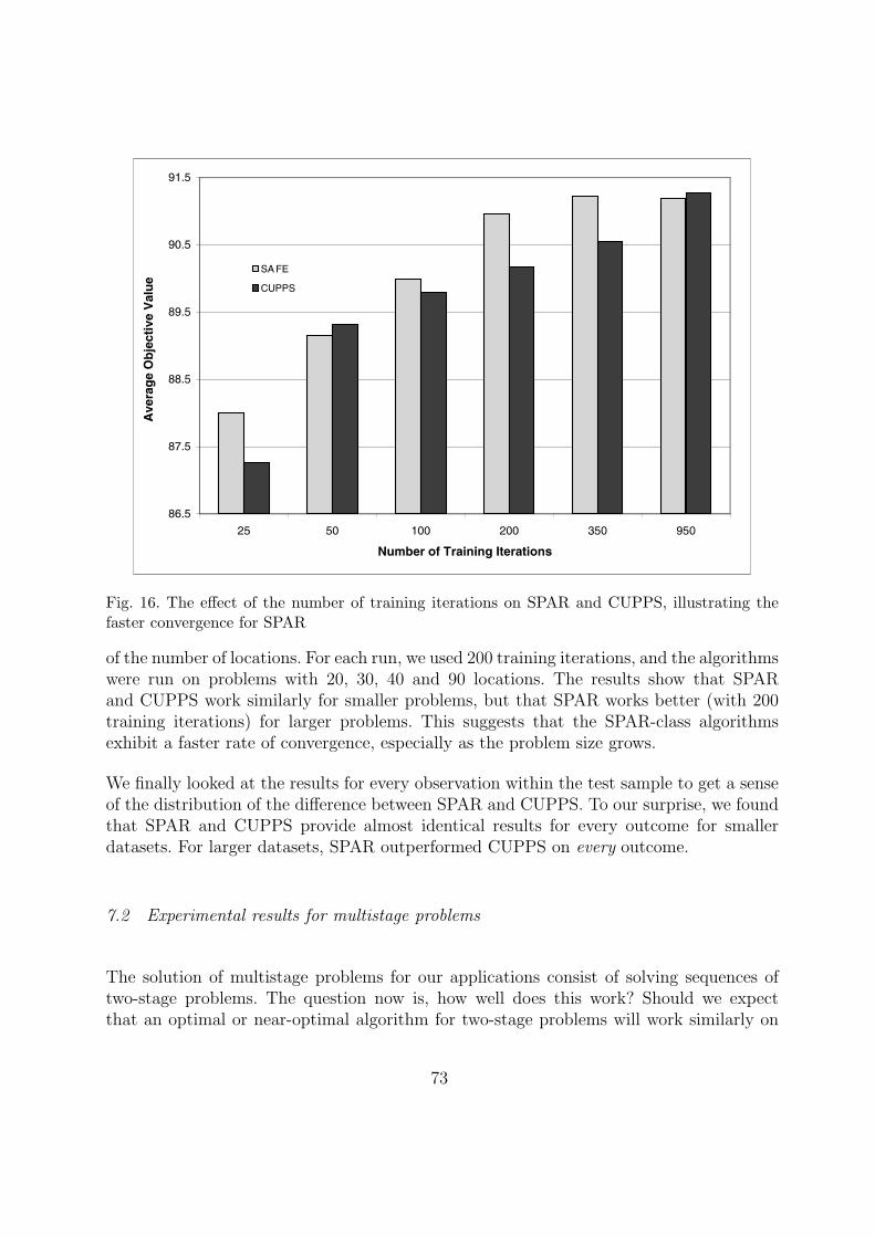
Fig. 16. The effect of the number of training iterations on SPAR and CUPPS, illustrating thefaster convergence for SPAR

of the number of locations. For each run, we used 200 training iterations, and the algorithmswere run on problems with 20, 30, 40 and 90 locations. The results show that SPARand CUPPS work similarly for smaller problems, but that SPAR works better (with 200training iterations) for larger problems. This suggests that the SPAR-class algorithmsexhibit a faster rate of convergence, especially as the problem size grows.

We finally looked at the results for every observation within the test sample to get a senseof the distribution of the difference between SPAR and CUPPS. To our surprise, we foundthat SPAR and CUPPS provide almost identical results for every outcome for smallerdatasets. For larger datasets, SPAR outperformed CUPPS on every outcome.

7.2 Experimental results for multistage problems

The solution of multistage problems for our applications consist of solving sequences oftwo-stage problems. The question now is, how well does this work? Should we expectthat an optimal or near-optimal algorithm for two-stage problems will work similarly on

73

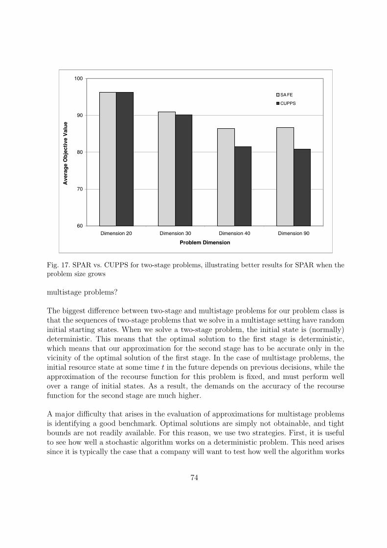
Fig. 17. SPAR vs. CUPPS for two-stage problems, illustrating better results for SPAR when theproblem size grows

multistage problems?

The biggest difference between two-stage and multistage problems for our problem class isthat the sequences of two-stage problems that we solve in a multistage setting have randominitial starting states. When we solve a two-stage problem, the initial state is (normally)deterministic. This means that the optimal solution to the first stage is deterministic,which means that our approximation for the second stage has to be accurate only in thevicinity of the optimal solution of the first stage. In the case of multistage problems, theinitial resource state at some time t in the future depends on previous decisions, while theapproximation of the recourse function for this problem is fixed, and must perform wellover a range of initial states. As a result, the demands on the accuracy of the recoursefunction for the second stage are much higher.

A major difficulty that arises in the evaluation of approximations for multistage problemsis identifying a good benchmark. Optimal solutions are simply not obtainable, and tightbounds are not readily available. For this reason, we use two strategies. First, it is usefulto see how well a stochastic algorithm works on a deterministic problem. This need arisessince it is typically the case that a company will want to test how well the algorithm works

74

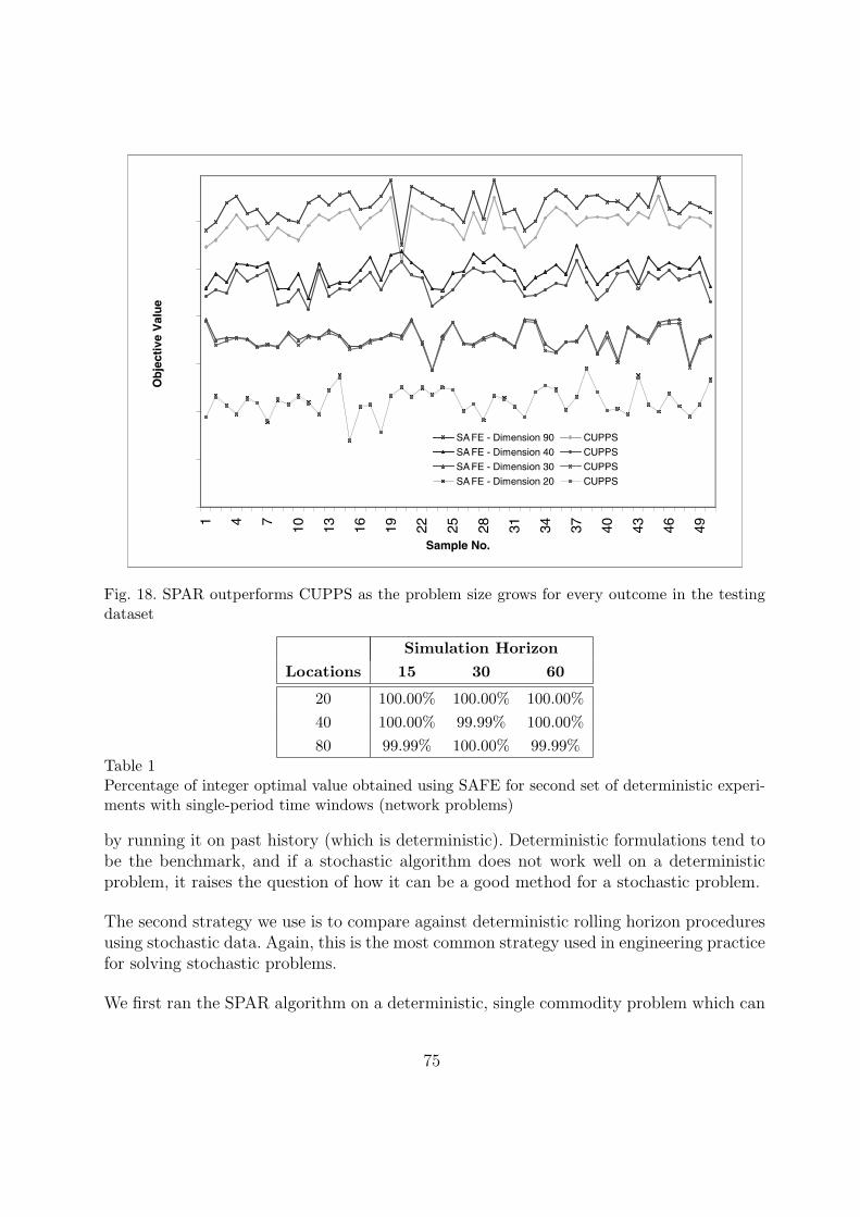
Fig. 18. SPAR outperforms CUPPS as the problem size grows for every outcome in the testingdataset

Simulation HorizonLocations 15 30 60

20 100.00% 100.00% 100.00%40 100.00% 99.99% 100.00%80 99.99% 100.00% 99.99%

Table 1Percentage of integer optimal value obtained using SAFE for second set of deterministic experi-ments with single-period time windows (network problems)

by running it on past history (which is deterministic). Deterministic formulations tend tobe the benchmark, and if a stochastic algorithm does not work well on a deterministicproblem, it raises the question of how it can be a good method for a stochastic problem.

The second strategy we use is to compare against deterministic rolling horizon proceduresusing stochastic data. Again, this is the most common strategy used in engineering practicefor solving stochastic problems.

We first ran the SPAR algorithm on a deterministic, single commodity problem which can

75

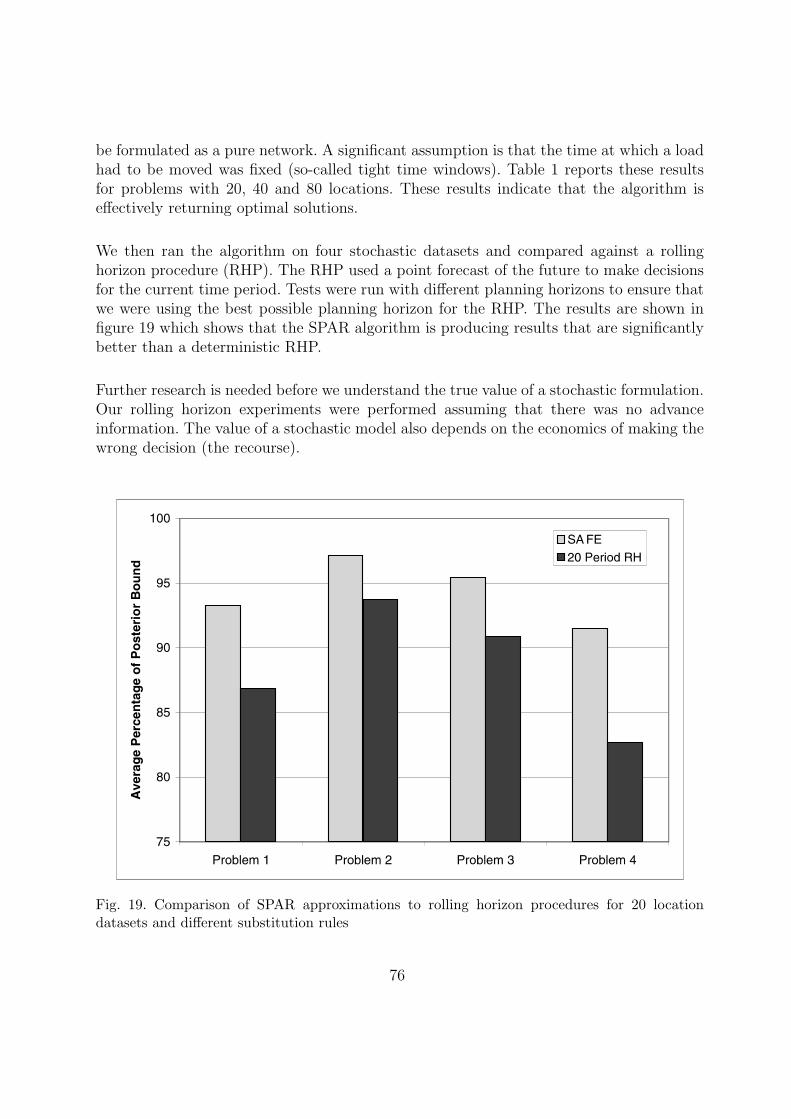
be formulated as a pure network. A significant assumption is that the time at which a loadhad to be moved was fixed (so-called tight time windows). Table 1 reports these resultsfor problems with 20, 40 and 80 locations. These results indicate that the algorithm iseffectively returning optimal solutions.

We then ran the algorithm on four stochastic datasets and compared against a rollinghorizon procedure (RHP). The RHP used a point forecast of the future to make decisionsfor the current time period. Tests were run with different planning horizons to ensure thatwe were using the best possible planning horizon for the RHP. The results are shown infigure 19 which shows that the SPAR algorithm is producing results that are significantlybetter than a deterministic RHP.

Further research is needed before we understand the true value of a stochastic formulation.Our rolling horizon experiments were performed assuming that there was no advanceinformation. The value of a stochastic model also depends on the economics of making thewrong decision (the recourse).

Fig. 19. Comparison of SPAR approximations to rolling horizon procedures for 20 locationdatasets and different substitution rules

76

8 A list of extensions

This chapter has introduced a basic problem class, discussing along the way practical algo-rithmic strategies, but steadily introducing issues that address the richness of transporta-tion problems. Our notational framework, which at first may seem clumsy to researchersaccustomed to even simpler notation, is designed to provide a natural bridge between theclassical notation of mathematical and stochastic programming, but provide for some ofthe issues that arise in practice. Our progression of problems, from two-stage to multistage,from single commodity with no substitution through multicommodity and heterogeneousresource allocation problems, was designed to bring the reader through a list of issues thatadd to the realism of the model being considered.

We have brought the reader to the edge of realistic problems that rise in practice, butreal problems of the type that arise in freight transportation have even more surprises todelight and frustrate the research community. In this section, we provide a hint of problemsthat remain to be addressed. All of the issues listed below represent forms of inaccurateinformation.

a) Random travel times - Not only are there multiperiod travel times, it is normally thecase that the travel time is random. A travel time may be uncertain even when a decisionis made.

b) Advance information - Customers place orders in advance. Railroads might let you knowthat they will give you empty cars in three days. A driver might tell you that he willstart in a week. We need to model the presence of information that is known, but notactionable.

c) Demand backlogging and the “now vs. later” problem - If we do not serve the customerrequest now, we may be able to serve it later (at a price). We can assign a driver toa distant load now, or wait for a closer load to be called in later. We need to identifywhen we should make a decision now (to serve a request) or wait until later.

d) Multiple, reusable layers - Perhaps the most challenging problem is the presence ofmultiple resource layers. (Recall that customer demands can also represent a kind ofresource layer). The simplest example arises with backlogging demands: if we do not servea demand now, it is still in the system in the next time period. In freight transportation,we may have to manage drivers, tractors and trailers, or locomotives, boxcars and crews.It is possible to model some freight transportation operations with four or five layers,and most of them are reusable.

e) User noncompliance - An overlooked dimension of most models is that what the modelis recommending is not what is being implemented. So the costs and contributions thatwe are adding up in the computer are not the costs and contributions we are getting inthe field. The difference between what a model recommends and what is implemented

77

in the field is a source of randomness that draws into question the value of so-calledoptimal solutions that ignore this source of randomness.

f) Multiagent control - Large problems are typically broken into smaller problems which aremanaged by different people. Decisions made by one person need to anticipate the impacton another. But it is impossible to predict what someone else will do with certainty. Thisis not the same as the user compliance problem, but it is another instance of solving aproblem where the randomness is in predicting what someone will do.

g) Data errors - We all know about data problems and recognize that we have to fix them,but we overlook the fact that the presence of data errors is again a source of noise.If data errors are going to require humans to override model recommendations, thenso-called “optimal” solutions are no longer optimal (even within a single stage).

h) Incomplete information - Random variables arise when we have information that isnot known now, but can be measured later. There are problems where information isunknown but can never be measured directly, which means we could never estimate aprobability distribution. But the missing information is captured in historical databasesof past decisions.

9 Implementing stochastic programming models in the real world

We close our discussion of stochastic problems by raising some of the issues that arisewhen we try to implement stochastic programming models in practice. In the beginningof this chapter, we made the argument that explicit models of uncertainty produce morerealistic behaviors, often exactly the behaviors that humans will mimic (perhaps with lessprecision) but deterministic models will overlook.

Humans have an innate ability to deal with imperfect information and noise. We allowmore time to make an appointment. We provide slack time in airline schedules to allowfor possible delays. We own extra trucks and locomotives to account for breakdowns,congestion and spikes in demand. Trucking companies have large rooms of people planningoperations who spend 90 percent of their time collecting and verifying data, and only 10percent actually making decisions. We would expect that planners would quickly embracemodels which capture the uncertainty that they spend so much time dealing with.

Surprisingly, this is not the case. Stochastic models arise because of the need to forecastan activity in the future, a forecast that is made with uncertainty. And yet in the businessworld, the word “forecast” is synonymous with the concept of a “point forecast.” Whenwe ask for a forecast of the number of box cars needed in a region next week, we do notwant to be told “somewhere between 70 and 100.” When we ask for a forecast, we expectan answer such as “85.”

78

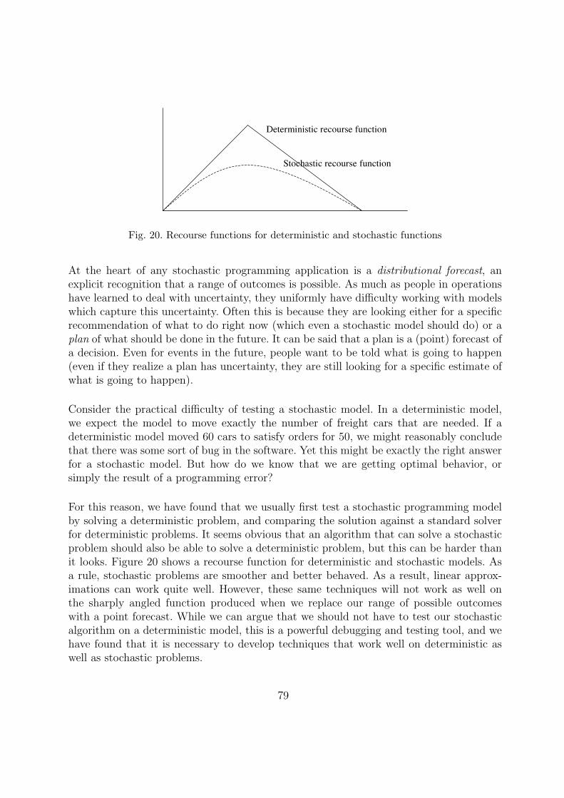
Fig. 20. Recourse functions for deterministic and stochastic functions

At the heart of any stochastic programming application is a distributional forecast, anexplicit recognition that a range of outcomes is possible. As much as people in operationshave learned to deal with uncertainty, they uniformly have difficulty working with modelswhich capture this uncertainty. Often this is because they are looking either for a specificrecommendation of what to do right now (which even a stochastic model should do) or aplan of what should be done in the future. It can be said that a plan is a (point) forecast ofa decision. Even for events in the future, people want to be told what is going to happen(even if they realize a plan has uncertainty, they are still looking for a specific estimate ofwhat is going to happen).

Consider the practical difficulty of testing a stochastic model. In a deterministic model,we expect the model to move exactly the number of freight cars that are needed. If adeterministic model moved 60 cars to satisfy orders for 50, we might reasonably concludethat there was some sort of bug in the software. Yet this might be exactly the right answerfor a stochastic model. But how do we know that we are getting optimal behavior, orsimply the result of a programming error?

For this reason, we have found that we usually first test a stochastic programming modelby solving a deterministic problem, and comparing the solution against a standard solverfor deterministic problems. It seems obvious that an algorithm that can solve a stochasticproblem should also be able to solve a deterministic problem, but this can be harder thanit looks. Figure 20 shows a recourse function for deterministic and stochastic models. Asa rule, stochastic problems are smoother and better behaved. As a result, linear approx-imations can work quite well. However, these same techniques will not work as well onthe sharply angled function produced when we replace our range of possible outcomeswith a point forecast. While we can argue that we should not have to test our stochasticalgorithm on a deterministic model, this is a powerful debugging and testing tool, and wehave found that it is necessary to develop techniques that work well on deterministic aswell as stochastic problems.

79

10 Bibliographic notes

The techniques in this chapter have their roots in stochastic approximation methods (Rob-bins & Monro (1951), Blum (1954), Dvoretzky (1956), Gladyshev (1965)), stochastic gradi-ent methods (Ermoliev (1988)), general stochastic linear programming (Birge & Louveaux(1997), Infanger (1994), Kall & Wallace (1994)) and dynamic programming (both classicalmethods, reviewed in Puterman (1994), and approximate methods, such as those coveredin Bertsekas & Tsitsiklis (1996), Sutton & Barto (1998)). For reviews of these topics, thereader is referred to the introductory chapters in this volume.

Applications in transportation and logistics represented some of the earliest motivationsfor stochastic programming. Dantzig (1955) used fleet management (in an airline setting)as an early motivation for stochastic programming. Ermoliev et al. (1976) formulated theplanning of empty shipping containers as a stochastic program.

There has been a rich history of research in fleet management in the context of the “cardistribution problem” of railroads. Most of this work consists of deterministic linear pro-gramming models (Feeney (1957), Leddon & Wrathall (1967), Gorenstein et al. (1971),Misra (1972), White (1972), Herren (1973), Herren (1977), White & Bomberault (1969),Haghani (1989), Mendiratta (1981), Mendiratta & Turnquist (1982)). Dejax & Crainic(1987) provide a thorough review of the research in fleet management at the time, cover-ing both rail and intermodal container applications. Crainic et al. (1993) provide a generalstochastic, dynamic model for container distribution.

Jordan & Turnquist (1983) provide a stochastic formulation of the empty car distributionproblem. In their model, a car could be assigned to at most one demand, and cars could notbe repositioned more than once. This structure allowed the problem to be formulated asa nonlinear programming problem. Powell (1986) extended this methodological approach,using the trucking industry as the context, to multistage problems with reusable resources.This formulation involved forming deterministic decision variables which specified the per-centage of the supply of trucks at a node that would be moved loaded or empty fromone location to another. This line of research, however, was unable to properly model therecourse strategy where a truck might be assigned to choose from a set of loads going outof a location to various destinations.

Powell (1987) solved this problem in a way that produced a pure network formulationfor the first stage subproblem (see Powell (1988) for an overview of different ways offormulating the problem). A major strength of the technique was that it produced nonlinearfunctions of the value of vehicles in the future. The ideas behind this research produceda series of articles that approximated the recourse function by using the structure ofthe underlying recourse function (Powell & Frantzeskakis (1992), Frantzeskakis & Powell

80

(1990), Powell & Cheung (1994b), Powell & Cheung (1994a), Cheung & Powell (1996)).These papers introduced concepts such as nodal recourse (the recourse is to allocate flowover different links out of a node), tree recourse (the recourse is to optimize flows overa tree) and other restricted recourse strategies aimed at approximating more complexproblems. Although the results were promising, this line of research required approximatingthe future in a way that prevented the techniques from being applied to the most general(and realistic) problems.

Powell & A. (1998) (see also Carvalho & Powell (2000)) took a different tact and solved theproblem as a sequence of network problems, using linear approximations of the value of thefuture. This approach was computationally quite easy, and scaled to much harder problems.Powell et al. (2002b) showed how the technique could be applied to the heterogeneousresource allocation problem, which is a more general problem than the multicommodityflow problem (the resource attribute space is much larger). The use of linear approximationsto represent the future, however, produced instabilities that were solved by the use ofcontrol variables that limited the amount of flow that could be moved from one locationto another. This worked very well for single commodity problems, but did not scale wellto multicommodity or heterogeneous resource allocation problems.

Godfrey & Powell (2001) introduce an adaptive sampling technique, dubbed the CAVEalgorithm, that produces nonlinear approximations of a recourse function using stochasticgradients. The method is easy to apply and produces piecewise linear, separable approx-imations of a recourse function. Furthermore, all it requires is the dual variable from asecond stage problem, and does not require that the problem have any particular structure.Experimental work suggested that the algorithm might be optimal for two-stage problems,but at a minimum it produced results that were extremely close to optimal for both de-terministic and specially structured stochastic problems. Godfrey & Powell (2002a) applyit to stochastic, multistage problems and demonstrate very good results relative to rollinghorizon procedures. Godfrey & Powell (2002b) investigated the case of resource alloca-tion where the travel time from one location to another can be multiple periods. A naiveapplication of the CAVE algorithm produced extremely poor results, and a variation issuggested that provides results that are comparable to the single period travel time case.

Topaloglu & Powell (2002) applies similar techniques to stochastic multicommodity flowproblems. This problem class introduces the additional complexity that multicommodityproblems, combined with nonlinear approximations of the future, produce sequences of(usually integer) multicommodity flow problems. The method appears to work well onboth both deterministic and multistage stochastic integer multicommodity flow problems.

The SPAR algorithm is part of a broader class of algorithms that use stochastic gradientsbut maintain structural properties such as concavity. This strategy was first suggested in

81

Godfrey & Powell (2001) as the CAVE algorithm, but the SPAR algorithm, introduced byPowell et al. (2002a), offers several provable convergence results and appears to also workbetter experimentally (see Topaloglu & Powell (2002) for the use of these techniques formultistage problems). Auxiliary function methods (Culioli & Cohen (1990) and Cheung &Powell (2000)) maintain concavity by starting with a concave function and using stochasticgradients to update the function (effectively tilting it).

References

Bertsekas, D. & Tsitsiklis, J. (1996), Neuro-Dynamic Programming, Athena Scientific,Belmont, MA.

Birge, J. & Louveaux, F. (1997), Introduction to Stochastic Programming, Springer-Verlag,New York.

Blum, J. (1954), ‘Multidimensional stochastic approximation methods’, Annals of Mathe-matical Statistics 25, 737–744.

Carvalho, T. A. & Powell, W. B. (2000), ‘A multiplier adjustment method for dynamicresource allocation problems’, Transportation Science 34, 150–164.

Cheung, R. & Powell, W. B. (1996), ‘An algorithm for multistage dynamic networks withrandom arc capacities, with an application to dynamic fleet management’, OperationsResearch 44(6), 951–963.

Cheung, R. K.-M. & Powell, W. B. (2000), ‘SHAPE: A stochastic hybrid approximationprocedure for two-stage stochastic programs’, Operations Research 48(1), 73–79.

Crainic, T., Gendreau, M. & Dejax, P. (1993), ‘Dynamic stochastic models for the alloca-tion of empty containers’, Operations Research 41, 102–126.

Culioli, J.-C. & Cohen, G. (1990), ‘Decomposition/coordination algorithms in stochasticoptimization’, SIAM Journal of Control and Optimization 28, 1372–1403.

Dantzig, G. (1955), ‘Linear programming under uncertainty’, Management Science 1, 197–206.

Dejax, P. & Crainic, T. (1987), ‘A review of empty flows and fleet management models infreight transportation’, Transportation Science 21, 227–247.

Dvoretzky, A. (1956), On stochastic approximation, in J. Neyman, ed., ‘Proc. 3rd BerkeleySym. on Math. Stat. and Prob.’, Berkeley: University of California Press, pp. 39–55.

Ermoliev, Y. (1988), Stochastic quasigradient methods, in Y. Ermoliev & R. Wets, eds,‘Numerical Techniques for Stochastic Optimization’, Springer-Verlag, Berlin.

Ermoliev, Y., Krivets, T. & Petukhov, V. (1976), ‘Planning of shipping empty seabornecontainers’, Cybernetics 12, 664.

Feeney, G. (1957), Controlling the distribution of empty cars, in ‘Proc. 10th NationalMeeting, Operations Research Society of America’.

Frantzeskakis, L. & Powell, W. B. (1990), ‘A successive linear approximation procedure forstochastic dynamic vehicle allocation problems’, Transportation Science 24(1), 40–57.

Gladyshev, E. G. (1965), ‘On stochastic approximation’, Theory of Prob. and its Appl.10, 275–278.

Godfrey, G. & Powell, W. B. (2002a), ‘An adaptive, dynamic programming algorithm forstochastic resource allocation problems I: Single period travel times’, TransportationScience 36(1), 21–39.

82

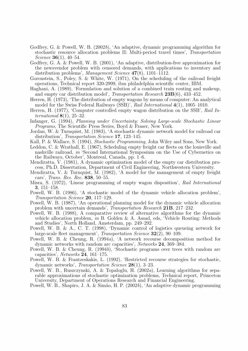
Godfrey, G. & Powell, W. B. (2002b), ‘An adaptive, dynamic programming algorithm forstochastic resource allocation problems II: Multi-period travel times’, TransportationScience 36(1), 40–54.

Godfrey, G. A. & Powell, W. B. (2001), ‘An adaptive, distribution-free approximation forthe newsvendor problem with censored demands, with applications to inventory anddistribution problems’, Management Science 47(8), 1101–1112.

Gorenstein, S., Poley, S. & White, W. (1971), On the scheduling of the railroad freightoperations, Technical report 320-2999, ibm philadelphia scientific center, IBM.

Haghani, A. (1989), ‘Formulation and solution of a combined train routing and makeup,and empty car distribution model’, Transportation Research 23B(6), 433–452.

Herren, H. (1973), ‘The distribution of empty wagons by means of computer: An analyticalmodel for the Swiss Federal Railways (SSB)’, Rail International 4(1), 1005–1010.

Herren, H. (1977), ‘Computer controlled empty wagon distribution on the SSB’, Rail In-ternational 8(1), 25–32.

Infanger, G. (1994), Planning under Uncertainty: Solving Large-scale Stochastic LinearPrograms, The Scientific Press Series, Boyd & Fraser, New York.

Jordan, W. & Turnquist, M. (1983), ‘A stochastic dynamic network model for railroad cardistribution’, Transportation Science 17, 123–145.

Kall, P. & Wallace, S. (1994), Stochastic Programming, John Wiley and Sons, New York.Leddon, C. & Wrathall, E. (1967), Scheduling empty freight car fleets on the louisville and

nashville railroad, in ‘Second International Symposium on the Use of Cybernetics onthe Railways, October’, Montreal, Canada, pp. 1–6.

Mendiratta, V. (1981), A dynamic optimization model of the empty car distribution pro-cess, Ph.D. Dissertation, Department of Civil Engineering, Northwestern University.

Mendiratta, V. & Turnquist, M. (1982), ‘A model for the management of empty freightcars’, Trans. Res. Rec. 838, 50–55.

Misra, S. (1972), ‘Linear programming of empty wagon disposition’, Rail International3, 151–158.

Powell, W. B. (1986), ‘A stochastic model of the dynamic vehicle allocation problem’,Transportation Science 20, 117–129.

Powell, W. B. (1987), ‘An operational planning model for the dynamic vehicle allocationproblem with uncertain demands’, Transportation Research 21B, 217–232.

Powell, W. B. (1988), A comparative review of alternative algorithms for the dynamicvehicle allocation problem, in B. Golden & A. Assad, eds, ‘Vehicle Routing: Methodsand Studies’, North Holland, Amsterdam, pp. 249–292.

Powell, W. B. & A., C. T. (1998), ‘Dynamic control of logistics queueing network forlarge-scale fleet management’, Transportation Science 32(2), 90–109.

Powell, W. B. & Cheung, R. (1994a), ‘A network recourse decomposition method fordynamic networks with random arc capacities’, Networks 24, 369–384.

Powell, W. B. & Cheung, R. (1994b), ‘Stochastic programs over trees with random arccapacities’, Networks 24, 161–175.

Powell, W. B. & Frantzeskakis, L. (1992), ‘Restricted recourse strategies for stochastic,dynamic networks’, Transportation Science 28(1), 3–23.

Powell, W. B., Ruszczynski, A. & Topaloglu, H. (2002a), Learning algorithms for sepa-rable approximations of stochastic optimization problems, Technical report, PrincetonUniversity, Department of Operations Research and Financial Engineering.

Powell, W. B., Shapiro, J. A. & Simao, H. P. (2002b), ‘An adaptive dynamic programming

83

algorithm for the heterogeneous resource allocation problem’, Transportation Science36(2), 231–249.

Puterman, M. L. (1994), Markov Decision Processes, John Wiley and Sons, Inc., NewYork.

Robbins, H. & Monro, S. (1951), ‘A stochastic approximation method’, Annals of Math.Stat. 22, 400–407.

Sutton, R. & Barto, A. (1998), Reinforcement Learning, The MIT Press, Cambridge, Mas-sachusetts.

Topaloglu, H. & Powell, W. B. (2002), Dynamic programming approximations for stochas-tic, time-staged integer multicommodity flow problems, Technical report, Princeton Uni-versity, Department of Operations Research and Financial Engineering.

White, W. (1972), ‘Dynamic transshipment networks: An algorithm and its application tothe distribution of empty containers’, Networks 2(3), 211–236.

White, W. & Bomberault, A. (1969), ‘A network algorithm for empty freight car alloca-tion’, IBM Systems Journal 8(2), 147–171.

84