stock evaluation of giant scallop (placopecten
TRANSCRIPT
Fisheries Research 60 (2003) 479–492
Stock evaluation of giant scallop (Placopecten magellanicus) usinghigh-resolution acoustics for seabed mapping
Vladimir E. Kostyleva,∗, Robert C. Courtneya, Ginette Robertb, Brian J. Toddaa Geological Survey of Canada (Atlantic), Bedford Institute of Oceanography, 1 Challenger Drive,
P.O. Box 1006, Dartmouth, NS, Canada B2Y 4A2b Invertebrate Fisheries Division, Bedford Institute of Oceanography, 1 Challenger Drive,
P.O. Box 1006, Dartmouth, NS, Canada B2Y 4A2
Received 6 March 2001; received in revised form 24 April 2002; accepted 9 May 2002
Abstract
Survey designs in use for the evaluation of sea scallop stocks do not consider the variability of sediment type, despite strongevidence of its importance for the recruitment and survival of scallops on the sea floor. This study examines the distributionof scallops on Browns Bank, Scotian Shelf, at two test sites, in comparison to sea floor sediment distribution, with particularattention to the effects of small-scale sediment variability on the abundance of the commercially exploited scallop. Importantlinks between scallop abundance, sediment type and habitat structure are described. Scallops are strongly associated withgravel lag deposits, which are readily distinguishable from sand-covered terrain through the use of multibeam backscatterdata. There exists a highly significant correlation between scallop survey catch rates and backscatter intensity which can beused for the prediction of scallop stock abundance. Developments in underwater acoustics enable for more precise sea floormapping and contribute to better estimates of scallop abundance.Crown Copyright © 2002 Published by Elsevier Science B.V. All rights reserved.
Keywords: Multibeam backscatter; Scallops;Placopecten magellanicus; Habitat; Benthos; Mapping
1. Introduction
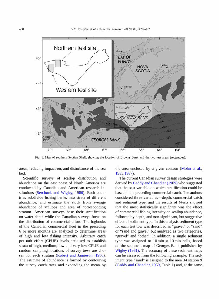
The Browns Bank sea scallop (Placopecten mag-ellanicus) fishery is one of the major Canadian scal-lop fisheries on the east coast, in operation sincethe early 1970s and continuing today. Currently, thelanded value of giant scallops constitutes one thirdof the total value of shellfish landed in the region.During the last three decades, the fishery has ex-ploited different parts of Browns Bank (Fig. 1) withan inconsistent rate of success. It is suspected that
∗ Corresponding author. Tel.:+1-902-426-8319;fax: +1-902-426-4104.E-mail address: [email protected] (V.E. Kostylev).
variable survival of juvenile scallops is responsiblefor considerable year-to-year changes in populationsize and landings. While recruitment into scalloppopulations cannot be controlled, accurate mappingof the distribution of commercial scallops can re-duce fishing effort and increase yield. The distribu-tion of adult scallops and recruitment of juvenileson the bank is very patchy. A better identificationof habitats suitable for scallop populations wouldlikely explain the patchy distribution of this bivalve.Increasing the accuracy of scallop distribution anddensity estimates based on maps of bottom habitatsmay lead to reducing effort in scallop fisheries andcould allow for better management of the resource,including planning of seed areas, marine protected
0165-7836/02/$ – see front matter. Crown Copyright © 2002 Published by Elsevier Science B.V. All rights reserved.PII: S0165-7836(02)00100-5
480 V.E. Kostylev et al. / Fisheries Research 60 (2003) 479–492
Fig. 1. Map of southern Scotian Shelf, showing the location of Browns Bank and the two test areas (rectangles).
areas, reducing impact on, and disturbance of the seabed.
Scientific surveys of scallop distribution andabundance on the east coast of North America areconducted by Canadian and American research in-stitutions (Serchuck and Wigley, 1986). Both coun-tries subdivide fishing banks into strata of differentabundance, and estimate the stock from averageabundance of scallops and area of correspondingstratum. American surveys base their stratificationon water depth while the Canadian surveys focus onthe distribution of commercial effort. The logbooksof the Canadian commercial fleet in the preceding6 or more months are analyzed to determine areasof high and low fishing intensity. Arbitrary catchper unit effort (CPUE) levels are used to establishstrata of high, medium, low and very low CPUE andrandom sampling locations of survey tows are cho-sen for each stratum (Robert and Jamieson, 1986).The estimate of abundance is formed by contouringthe survey catch rates and expanding the mean by
the area enclosed by a given contour (Mohn et al.,1985,1987).
The current Canadian survey design strategies werederived byCaddy and Chandler (1969)who suggestedthat the best variable on which stratification could bebased is the preceding commercial catch. The authorsconsidered three variables—depth, commercial catchand sediment type, and the results oft-tests showedthat the most statistically significant was the effectof commercial fishing intensity on scallop abundance,followed by depth, and non-significant, but suggestiveeffect of sediment type. In this analysis sediment typefor each test tow was described as “gravel” or “sand”or “sand and gravel” but analyzed as two categories,“gravel” and “other”. In addition, a single sedimenttype was assigned to 10 min× 10 min cells, basedon the sediment map of Georges Bank published byWigley (1961). The accuracy of these sediment mapscan be assessed from the following example. The sed-iment type “sand” is assigned to the area 34 station 9(Caddy and Chandler, 1969, Table 1) and, at the same
V.E. Kostylev et al. / Fisheries Research 60 (2003) 479–492 481
time, the comment for this station is “too rocky tofish” (Caddy and Chandler, 1969, Table 3).
Comparison of American and Canadian surveydesigns has shown that they are relatively equal in per-formance (Serchuck and Wigley, 1986). Evaluation ofthe relative ability of these designs to estimate the ac-tual scallop abundance would necessitate developmentof a third technique against which these two designscould be evaluated (Robert and Jamieson, 1986).
General knowledge about scallop ecology and dis-tribution matches the occurrence of scallops withsand and gravel sediments (e.g.Bousfield, 1960). Thestudy of benthic habitats on Browns Bank (Kostylevet al., 2001), based on the analysis of underwaterphotographs similarly showed that scallops dwell ingravelly areas, with a smooth seabed and higher thanaverage current speeds.Smith and Robert (1998)sug-gested that allocation of sediment type strata withineach of the commercial catch strata would likelyprovide some gains in precision of stock estimatescompared to random sampling design. The resultswere based on the analysis of Georges Bank scallopcatches, and simplified map of surficial sedimentsfrom Thouseau et al. (1991). The term “surficial”means “pertaining to, situated at, or formed or occur-ring on a surface, especially the surface of the earth”(Gary et al., 1977).
New research evolving out of the application ofmultibeam bathymetric systems (Todd et al., 1999)has shown that the surficial sediment distributionon Browns Bank is more complex than previouslymapped and that overly generalized maps of sedi-ments distribution were not suitable for correlationwith fishery catch statistics. Geological mapping ofBrowns Bank, performed by Geological Survey ofCanada (Atlantic) on the basis of multibeam imageryand a suite of ground truthing methods, has been usedto identify areas of sand cover and gravel lag. Themapping was carried out to an areal resolution gener-ally less than 10 m× 10 m, an increase in resolutionby a factor greater than 1000 compared to existingmaps. Considering the previous knowledge about theeffects of sediment type on recruitment and survivalof sea scallops, it seems appropriate to re-evaluate thecurrent survey techniques, given the new sedimentinformation.
The current study examines the distribution of scal-lops in comparison to sea floor sediment distribu-
tion, as predicted using an acoustic backscatter proxy,with particular attention focussed on the effects ofsmall-scale sediment variability on the estimation ofscallop abundance. We describe links between scallopabundance, sediment type and habitat structure, andpropose that sediment type should be the dominant fac-tor in the design of research surveys of scallop stocks.
2. Methods
Multibeam bathymetric data were collected by theCanadian Hydrographic Service on Browns Bank in1996 and 1997 using the CCGS Frederick G. Creedequipped with a 95 kHz Simrad EM1000 multibeambathymetric system. This system produces 60 narrowbeams with average rate of 5 pings per second fan-ning over an arc of 150◦ and operates by ensonifyinga narrow strip of sea floor across the beam of the sur-vey vessel and detecting the bottom echo with narrow,across-track listening beams. The swath of sea floorimaged on each survey line is typically 5–6 times thewater depth in 100 m water depth. In the Browns Banksurveys, line spacing was about 3–4 times water depthto provide complete ensonification overlap betweenadjacent lines. Navigation was by Differential GlobalPositioning System, providing positional accuracy of±3 m. Survey speeds averaged 14 knots resulting inan average data collection rate of about 5.0 km2/h inwater depths of 35–70 m.
During the survey, water depth values were in-spected and erroneous values were removed usingCARIS/Hydrographic Information Processing System(HIPS) software from Universal Systems Limited,Fredericton, NB. Within HIPS, the data were adjustedfor tidal variation using tidal predictions from theCanadian Hydrographic Service. Multibeam bathy-metric data were gridded in 5–10 m (horizontal) binsand shaded with artificial illumination using softwaredeveloped by the Ocean Mapping Group at the Ge-ological Survey of Canada (Atlantic). Relief maps,color-coded to depth were developed and displayedon a Hewlett-Packard workstation using GRASS(Geographic Resources Analysis Support System)developed at the US Army Construction EngineeringResearch Laboratories.
In addition to the bathymetric data, calibratedacoustic backscatter data can be logged by the Simrad
482 V.E. Kostylev et al. / Fisheries Research 60 (2003) 479–492
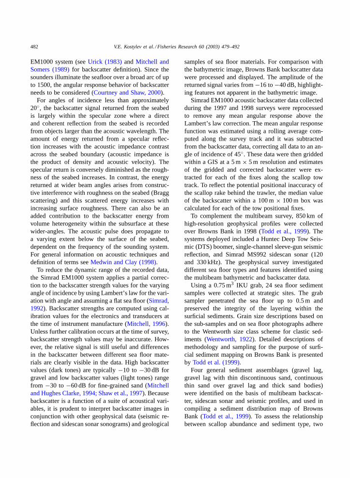
EM1000 system (seeUrick (1983)andMitchell andSomers (1989)for backscatter definition). Since thesounders illuminate the seafloor over a broad arc of upto 1500, the angular response behavior of backscatterneeds to be considered (Courtney and Shaw, 2000).
For angles of incidence less than approximately20◦, the backscatter signal returned from the seabedis largely within the specular zone where a directand coherent reflection from the seabed is recordedfrom objects larger than the acoustic wavelength. Theamount of energy returned from a specular reflec-tion increases with the acoustic impedance contrastacross the seabed boundary (acoustic impedance isthe product of density and acoustic velocity). Thespecular return is conversely diminished as the rough-ness of the seabed increases. In contrast, the energyreturned at wider beam angles arises from construc-tive interference with roughness on the seabed (Braggscattering) and this scattered energy increases withincreasing surface roughness. There can also be anadded contribution to the backscatter energy fromvolume heterogeneity within the subsurface at thesewider-angles. The acoustic pulse does propagate toa varying extent below the surface of the seabed,dependent on the frequency of the sounding system.For general information on acoustic techniques anddefinition of terms seeMedwin and Clay (1998).
To reduce the dynamic range of the recorded data,the Simrad EM1000 system applies a partial correc-tion to the backscatter strength values for the varyingangle of incidence by using Lambert’s law for the vari-ation with angle and assuming a flat sea floor (Simrad,1992). Backscatter strengths are computed using cal-ibration values for the electronics and transducers atthe time of instrument manufacture (Mitchell, 1996).Unless further calibration occurs at the time of survey,backscatter strength values may be inaccurate. How-ever, the relative signal is still useful and differencesin the backscatter between different sea floor mate-rials are clearly visible in the data. High backscattervalues (dark tones) are typically−10 to −30 dB forgravel and low backscatter values (light tones) rangefrom −30 to −60 dB for fine-grained sand (Mitchelland Hughes Clarke, 1994; Shaw et al., 1997). Becausebackscatter is a function of a suite of acoustical vari-ables, it is prudent to interpret backscatter images inconjunction with other geophysical data (seismic re-flection and sidescan sonar sonograms) and geological
samples of sea floor materials. For comparison withthe bathymetric image, Browns Bank backscatter datawere processed and displayed. The amplitude of thereturned signal varies from−16 to−40 dB, highlight-ing features not apparent in the bathymetric image.
Simrad EM1000 acoustic backscatter data collectedduring the 1997 and 1998 surveys were reprocessedto remove any mean angular response above theLambert’s law correction. The mean angular responsefunction was estimated using a rolling average com-puted along the survey track and it was subtractedfrom the backscatter data, correcting all data to an an-gle of incidence of 45◦. These data were then griddedwithin a GIS at a 5 m× 5 m resolution and estimatesof the gridded and corrected backscatter were ex-tracted for each of the fixes along the scallop towtrack. To reflect the potential positional inaccuracy ofthe scallop rake behind the trawler, the median valueof the backscatter within a 100 m× 100 m box wascalculated for each of the tow positional fixes.
To complement the multibeam survey, 850 km ofhigh-resolution geophysical profiles were collectedover Browns Bank in 1998 (Todd et al., 1999). Thesystems deployed included a Huntec Deep Tow Seis-mic (DTS) boomer, single-channel sleeve-gun seismicreflection, and Simrad MS992 sidescan sonar (120and 330 kHz). The geophysical survey investigateddifferent sea floor types and features identified usingthe multibeam bathymetric and backscatter data.
Using a 0.75 m3 IKU grab, 24 sea floor sedimentsamples were collected at strategic sites. The grabsampler penetrated the sea floor up to 0.5 m andpreserved the integrity of the layering within thesurficial sediments. Grain size descriptions based onthe sub-samples and on sea floor photographs adhereto the Wentworth size class scheme for clastic sed-iments (Wentworth, 1922). Detailed descriptions ofmethodology and sampling for the purpose of surfi-cial sediment mapping on Browns Bank is presentedby Todd et al. (1999).
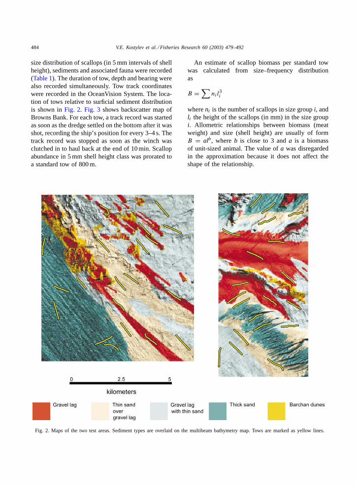
Four general sediment assemblages (gravel lag,gravel lag with thin discontinuous sand, continuousthin sand over gravel lag and thick sand bodies)were identified on the basis of multibeam backscat-ter, sidescan sonar and seismic profiles, and used incompiling a sediment distribution map of BrownsBank (Todd et al., 1999). To assess the relationshipbetween scallop abundance and sediment type, two
V.E. Kostylev et al. / Fisheries Research 60 (2003) 479–492 483
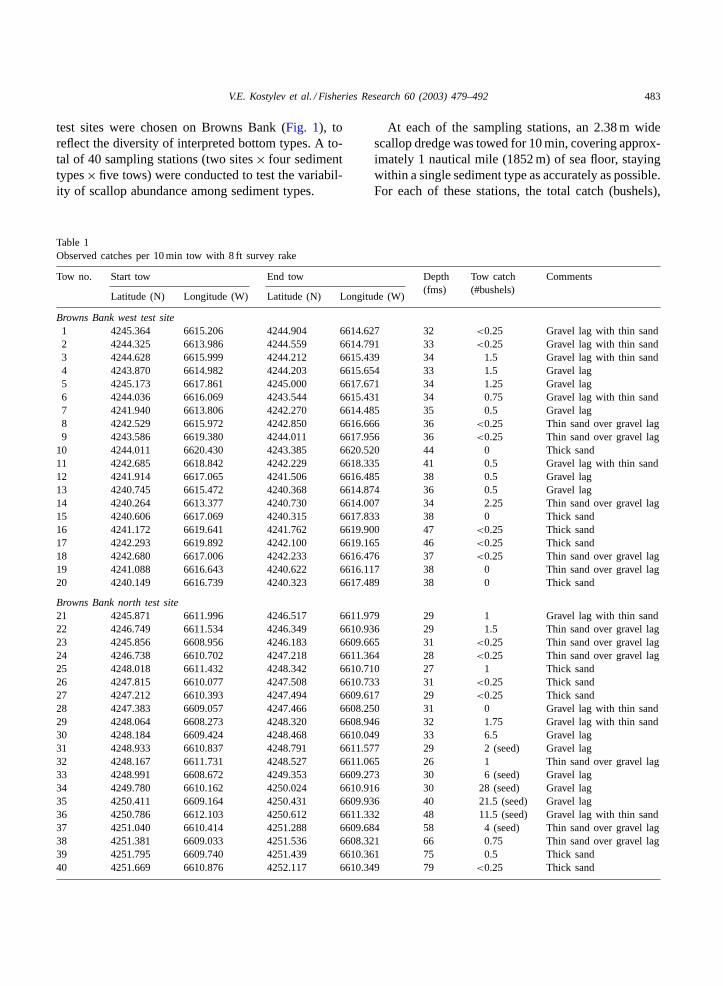
test sites were chosen on Browns Bank (Fig. 1), toreflect the diversity of interpreted bottom types. A to-tal of 40 sampling stations (two sites× four sedimenttypes× five tows) were conducted to test the variabil-ity of scallop abundance among sediment types.
Table 1Observed catches per 10 min tow with 8 ft survey rake
Tow no. Start tow End tow Depth(fms)
Tow catch(#bushels)
Comments
Latitude (N) Longitude (W) Latitude (N) Longitude (W)
Browns Bank west test site1 4245.364 6615.206 4244.904 6614.627 32 <0.25 Gravel lag with thin sand2 4244.325 6613.986 4244.559 6614.791 33 <0.25 Gravel lag with thin sand3 4244.628 6615.999 4244.212 6615.439 34 1.5 Gravel lag with thin sand4 4243.870 6614.982 4244.203 6615.654 33 1.5 Gravel lag5 4245.173 6617.861 4245.000 6617.671 34 1.25 Gravel lag6 4244.036 6616.069 4243.544 6615.431 34 0.75 Gravel lag with thin sand7 4241.940 6613.806 4242.270 6614.485 35 0.5 Gravel lag8 4242.529 6615.972 4242.850 6616.666 36 <0.25 Thin sand over gravel lag9 4243.586 6619.380 4244.011 6617.956 36 <0.25 Thin sand over gravel lag
10 4244.011 6620.430 4243.385 6620.520 44 0 Thick sand11 4242.685 6618.842 4242.229 6618.335 41 0.5 Gravel lag with thin sand12 4241.914 6617.065 4241.506 6616.485 38 0.5 Gravel lag13 4240.745 6615.472 4240.368 6614.874 36 0.5 Gravel lag14 4240.264 6613.377 4240.730 6614.007 34 2.25 Thin sand over gravel lag15 4240.606 6617.069 4240.315 6617.833 38 0 Thick sand16 4241.172 6619.641 4241.762 6619.900 47 <0.25 Thick sand17 4242.293 6619.892 4242.100 6619.165 46 <0.25 Thick sand18 4242.680 6617.006 4242.233 6616.476 37 <0.25 Thin sand over gravel lag19 4241.088 6616.643 4240.622 6616.117 38 0 Thin sand over gravel lag20 4240.149 6616.739 4240.323 6617.489 38 0 Thick sand
Browns Bank north test site21 4245.871 6611.996 4246.517 6611.979 29 1 Gravel lag with thin sand22 4246.749 6611.534 4246.349 6610.936 29 1.5 Thin sand over gravel lag23 4245.856 6608.956 4246.183 6609.665 31 <0.25 Thin sand over gravel lag24 4246.738 6610.702 4247.218 6611.364 28 <0.25 Thin sand over gravel lag25 4248.018 6611.432 4248.342 6610.710 27 1 Thick sand26 4247.815 6610.077 4247.508 6610.733 31 <0.25 Thick sand27 4247.212 6610.393 4247.494 6609.617 29 <0.25 Thick sand28 4247.383 6609.057 4247.466 6608.250 31 0 Gravel lag with thin sand29 4248.064 6608.273 4248.320 6608.946 32 1.75 Gravel lag with thin sand30 4248.184 6609.424 4248.468 6610.049 33 6.5 Gravel lag31 4248.933 6610.837 4248.791 6611.577 29 2 (seed) Gravel lag32 4248.167 6611.731 4248.527 6611.065 26 1 Thin sand over gravel lag33 4248.991 6608.672 4249.353 6609.273 30 6 (seed) Gravel lag34 4249.780 6610.162 4250.024 6610.916 30 28 (seed) Gravel lag35 4250.411 6609.164 4250.431 6609.936 40 21.5 (seed) Gravel lag36 4250.786 6612.103 4250.612 6611.332 48 11.5 (seed) Gravel lag with thin sand37 4251.040 6610.414 4251.288 6609.684 58 4 (seed) Thin sand over gravel lag38 4251.381 6609.033 4251.536 6608.321 66 0.75 Thin sand over gravel lag39 4251.795 6609.740 4251.439 6610.361 75 0.5 Thick sand40 4251.669 6610.876 4252.117 6610.349 79 <0.25 Thick sand
At each of the sampling stations, an 2.38 m widescallop dredge was towed for 10 min, covering approx-imately 1 nautical mile (1852 m) of sea floor, stayingwithin a single sediment type as accurately as possible.For each of these stations, the total catch (bushels),
484 V.E. Kostylev et al. / Fisheries Research 60 (2003) 479–492
size distribution of scallops (in 5 mm intervals of shellheight), sediments and associated fauna were recorded(Table 1). The duration of tow, depth and bearing werealso recorded simultaneously. Tow track coordinateswere recorded in the OceanVision System. The loca-tion of tows relative to surficial sediment distributionis shown inFig. 2. Fig. 3 shows backscatter map ofBrowns Bank. For each tow, a track record was startedas soon as the dredge settled on the bottom after it wasshot, recording the ship’s position for every 3–4 s. Thetrack record was stopped as soon as the winch wasclutched in to haul back at the end of 10 min. Scallopabundance in 5 mm shell height class was prorated toa standard tow of 800 m.
Fig. 2. Maps of the two test areas. Sediment types are overlaid on the multibeam bathymetry map. Tows are marked as yellow lines.
An estimate of scallop biomass per standard towwas calculated from size–frequency distributionas
B =∑
nil3i
whereni is the number of scallops in size groupi, andli the height of the scallops (in mm) in the size groupi. Allometric relationships between biomass (meatweight) and size (shell height) are usually of formB = alb, whereb is close to 3 anda is a biomassof unit-sized animal. The value ofa was disregardedin the approximation because it does not affect theshape of the relationship.
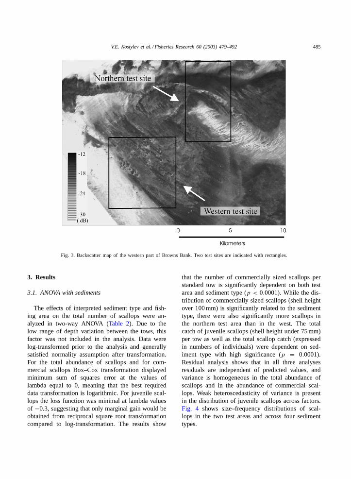
V.E. Kostylev et al. / Fisheries Research 60 (2003) 479–492 485
Fig. 3. Backscatter map of the western part of Browns Bank. Two test sites are indicated with rectangles.
3. Results
3.1. ANOVA with sediments
The effects of interpreted sediment type and fish-ing area on the total number of scallops were an-alyzed in two-way ANOVA (Table 2). Due to thelow range of depth variation between the tows, thisfactor was not included in the analysis. Data werelog-transformed prior to the analysis and generallysatisfied normality assumption after transformation.For the total abundance of scallops and for com-mercial scallops Box–Cox transformation displayedminimum sum of squares error at the values oflambda equal to 0, meaning that the best requireddata transformation is logarithmic. For juvenile scal-lops the loss function was minimal at lambda valuesof −0.3, suggesting that only marginal gain would beobtained from reciprocal square root transformationcompared to log-transformation. The results show
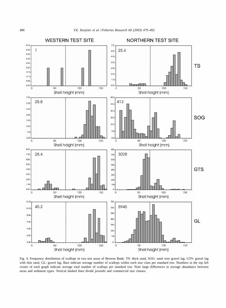
that the number of commercially sized scallops perstandard tow is significantly dependent on both testarea and sediment type (p < 0.0001). While the dis-tribution of commercially sized scallops (shell heightover 100 mm) is significantly related to the sedimenttype, there were also significantly more scallops inthe northern test area than in the west. The totalcatch of juvenile scallops (shell height under 75 mm)per tow as well as the total scallop catch (expressedin numbers of individuals) were dependent on sed-iment type with high significance (p = 0.0001).Residual analysis shows that in all three analysesresiduals are independent of predicted values, andvariance is homogeneous in the total abundance ofscallops and in the abundance of commercial scal-lops. Weak heteroscedasticity of variance is presentin the distribution of juvenile scallops across factors.Fig. 4 shows size–frequency distributions of scal-lops in the two test areas and across four sedimenttypes.
486 V.E. Kostylev et al. / Fisheries Research 60 (2003) 479–492
Fig. 4. Frequency distribution of scallops in two test areas of Browns Bank. TS: thick sand, SOG: sand over gravel lag, GTS: gravel lagwith thin sand, GL: gravel lag. Bars indicate average number of scallops within each size class per standard tow. Numbers in the top leftcorner of each graph indicate average total number of scallops per standard tow. Note large differences in average abundance betweenareas and sediment types. Vertical dashed lines divide juvenile and commercial size classes.
V.E. Kostylev et al. / Fisheries Research 60 (2003) 479–492 487
Table 2Summary of all effects of ANOVA, performed on abundances of size groups in the total catcha
d.f. effect MS effect d.f. error MS error F p-level
Total number of scallops per standard towTest site 1 12.6801633 32 0.6537382 19.396392 0.000111Sediment 3 6.32045412 32 0.6537382 9.6681728 0.000107Interaction 3 1.00208318 32 0.6537382 1.5328508 0.224910
Number of commercial size scallops per standard towTest site 1 8.25006294 32 0.5114458 16.130863 0.000334Sediment 3 5.34637737 32 0.5114458 10.453456 0.000059Interaction 3 0.72987085 32 0.5114458 1.4270734 0.253019
Number of juvenile scallops per standard towTest site 1 18.4019241 32 0.7148605 25.741977 0.000015Sediment 3 4.07664299 32 0.7148605 5.7027106 0.003031Interaction 3 2.64774751 32 0.7148605 3.7038657 0.021479
a The ANOVA model accounted for 62.4% variability in total catch of scallops, 61.8% in abundance of commercial scallops and62.8% in abundance of juvenile scallops. Sediment type explained 34% of variance in total abundance of scallops, 38% in abundance ofcommercial scallops and 20% in juvenile scallops.
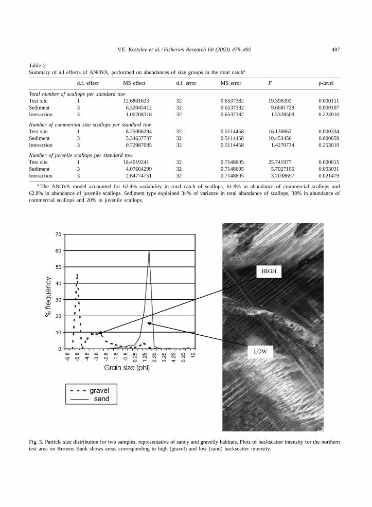
Fig. 5. Particle size distribution for two samples, representative of sandy and gravelly habitats. Plots of backscatter intensity for the northerntest area on Browns Bank shows areas corresponding to high (gravel) and low (sand) backscatter intensity.
488 V.E. Kostylev et al. / Fisheries Research 60 (2003) 479–492
3.2. Backscatter and sediment particle size
The sediment distribution mapping was largelybased on the acoustic backscatter of sea floor, whichmakes it possible, among other things, to distinguishbetween coarse-grained and fine-grained sediment.Seafloor sediment samples allowed the correlation ofparticle size distribution to backscatter values.Fig. 5shows typical particle size distributions for graveland sandy habitats and their relation to backscat-ter intensity. The dark tones inFig. 5 correspondto high backscatter (gravel) and the light tonesto low backscatter (sand). We interpret backscat-ter maps to represent continuous variation in sed-iment structure, and the current study is the firstprecedent of the use of backscatter values for nu-merical analysis of scallop distribution. The useof backscatter strength for correlation with scallopcatch allowed to avoid unaccounted variability in
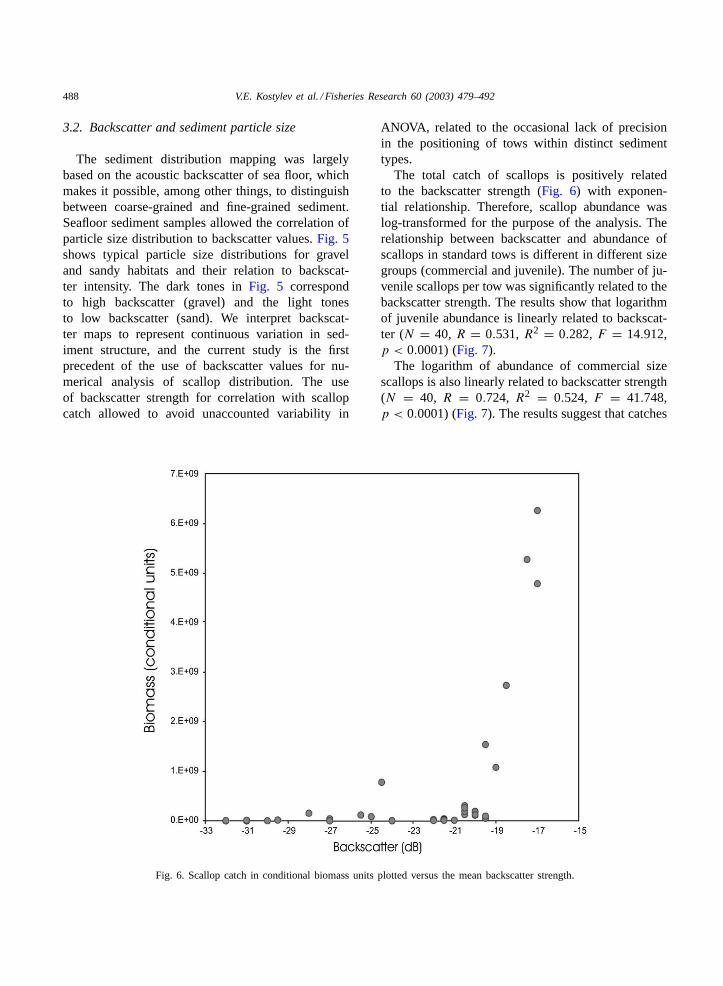
Fig. 6. Scallop catch in conditional biomass units plotted versus the mean backscatter strength.
ANOVA, related to the occasional lack of precisionin the positioning of tows within distinct sedimenttypes.
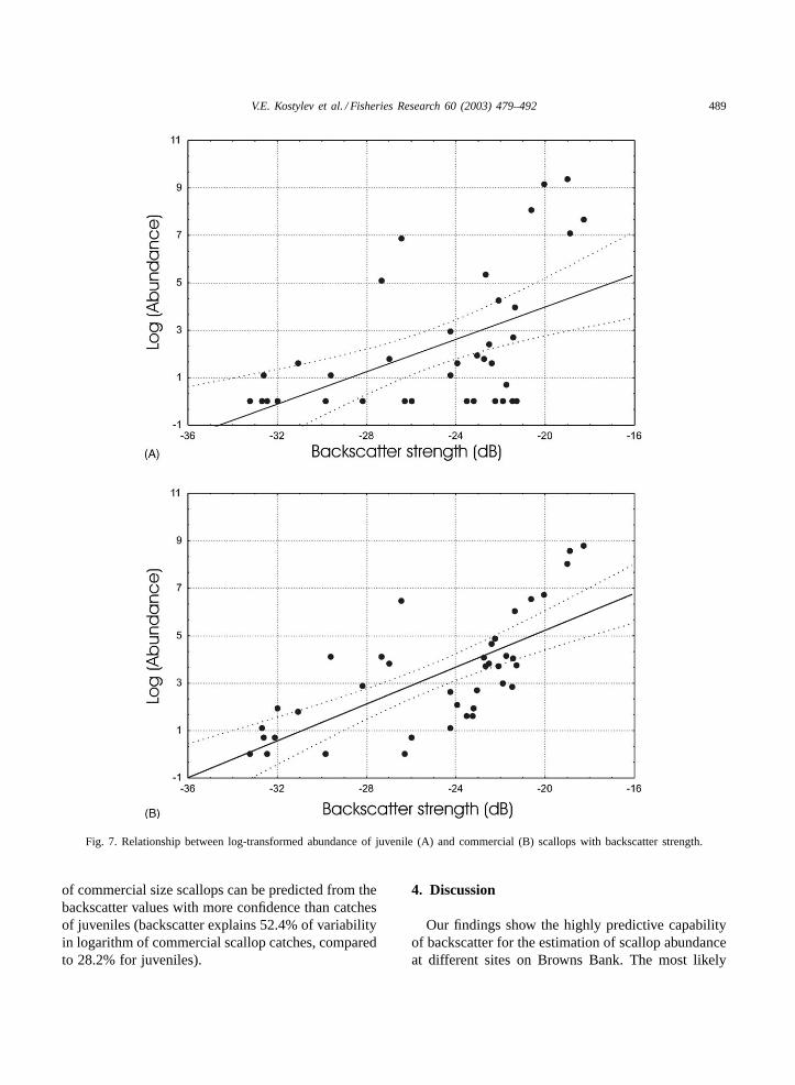
The total catch of scallops is positively relatedto the backscatter strength (Fig. 6) with exponen-tial relationship. Therefore, scallop abundance waslog-transformed for the purpose of the analysis. Therelationship between backscatter and abundance ofscallops in standard tows is different in different sizegroups (commercial and juvenile). The number of ju-venile scallops per tow was significantly related to thebackscatter strength. The results show that logarithmof juvenile abundance is linearly related to backscat-ter (N = 40, R = 0.531,R2 = 0.282,F = 14.912,p < 0.0001) (Fig. 7).
The logarithm of abundance of commercial sizescallops is also linearly related to backscatter strength(N = 40, R = 0.724, R2 = 0.524, F = 41.748,p < 0.0001) (Fig. 7). The results suggest that catches
V.E. Kostylev et al. / Fisheries Research 60 (2003) 479–492 489
Fig. 7. Relationship between log-transformed abundance of juvenile (A) and commercial (B) scallops with backscatter strength.
of commercial size scallops can be predicted from thebackscatter values with more confidence than catchesof juveniles (backscatter explains 52.4% of variabilityin logarithm of commercial scallop catches, comparedto 28.2% for juveniles).
4. Discussion
Our findings show the highly predictive capabilityof backscatter for the estimation of scallop abundanceat different sites on Browns Bank. The most likely
490 V.E. Kostylev et al. / Fisheries Research 60 (2003) 479–492
reason of this high correlation is the life historytraits of juvenile scallops, namely the requirements ofscallop larvae for metamorphosis, which is a criticalevent in a molluscan life history. The transition froma pelagic to a benthic existence is accompanied bychanges in diet and morphology (disappearance ofthe velum and attachment by byssus). Settlement isa pre-requisite for metamorphosis and if a suitablesubstrate is not found then the larva may die. Scalloplarvae have a strong tendency to settle on the under-side of pebbles and shell hash (Culliney, 1974). Set-tling under such conditions would offer some safetyfor the larva against predators. Scallop also settle onbiogenic structures such as red algae, hydrozoa andbryozoa. The shallow part of Browns Bank is pri-marily a lag gravel, often covered with hydroids andbryozoans (Kostylev et al., 2001), making this habitatparticularly suitable for juvenile scallops.
The relative proportion of commercial scallops washigher in the western test site, where the recruitment isimpeded by the lack of available substrate. It is likelythat a large area with sandy substrates makes it diffi-cult for seed to attach. On thick sand, in the northerntest site, the commercial size scallops are more abun-dant than juveniles. This may be explained by the verystrong current in this area, which could sweep away orbury the smaller scallops in the sand. While the adultscallops are also found mostly on gravel, they are prob-ably able to disperse to a certain extent and survive insandy habitats better than juveniles are. Thus, changesin relative proportions of juvenile and commercialscallops can be easily explained by the preference ofjuvenile scallops to settle on gravelly sediments.
The scallop habitat of Browns Bank is generallypoor in other megafauna species. Typical species as-sociated with scallops are hydroidea, especiallySer-tularella sp., which is common and often attached toscallop shells (Kostylev et al., 2001). Carnivores suchas whelks and hermit crabs are common and probablyderive food supply from damage to benthic speciesdamaged by scallop dredging (Caddy, 1970).
The wide applicability of the relationship betweenbackscatter and scallop abundance has to be tested inconsideration to other important environmental factorsthat would certainly influence scallops distribution.Water depth, food supply, temperature range, preda-tion pressure, disturbance by fishing activities—allcan influence the resulting pattern of scallop distribu-
tion. On Browns Bank, scallops were found in highestdensities on gravel substrate on the western part ofthe bank. The presence of strong currents for larvaldispersion and gravel for larval settlement (Bousfield,1960), combined with optimum shallow water depths(Miner, 1950), make this area ideal for scallop recruit-ment. Water masses over the western part of the bankprovide scallops with abundant phytoplankton, whichis a primary source of scallop food (Cranford andGrant, 1990). In contrast, the deeper eastern part ofthe bank, with the presence of fine-grained sedimentsand possibly periodic resuspension of detritus is lesssuitable for scallop recruitment and establishment oflarge populations. Scallop spat is highly susceptibleto siltation (Dickie and Medcof, 1956) and silt cancause adult mortality, in part through the cloggingof cilia on the gills (Larsen and Lee, 1978; Cranfordand Gordon, 1992). In addition, inorganic sedimentreduces the energetic quality of ingested food thuslimiting productivity of the population. The maxi-mum densities of scallops on the bank were generallyfound at depths of 70–90 m on gravel lag or gravellag with thin, discontinuous sand (Kostylev et al.,2001).
There exists no direct and simple relationship be-tween the backscatter amplitude and surficial sedimenttexture. Generally for angles outside the specularrange, there does exist a general correspondence be-tween backscatter amplitudes and surficial sedimentroughness that can be used for cursory mapping andsediment identification. Coarse gravels and cobblestend to be locally rough and return high-amplitude,wide-angle backscatter signals, whereas sands andfine-grained materials can be locally smooth with amuch lower backscatter. Care must be taken to lookat the complete angular response of backscatter insome cases. Flat or polished bedrock, e.g., is locallysmooth and thus can have a very low wide-anglebackscatter response, which could be confused withclay or other smooth, fine-grained deposits. The nearnadir response would, in this instance, be needed todifferentiate the two possibilities. Coincident seismicdata and seabed samples are often collected to aidthe backscatter interpretation. Meanwhile, backscatterstrength may serve as a proxy for a variety of dy-namic factors taking place at seabed surface. Indeed,the sediments are often indicative of the dynamics ofnear-bottom flows, which may define both sediment
V.E. Kostylev et al. / Fisheries Research 60 (2003) 479–492 491
grain size and benthic community structure (Jumars,1993; Wildish and Kristmanson, 1997).
Current stock assessment techniques underestimatespatial trends in environmental variables, such assediment type. In Canadian scallop surveys samplingintensity is disproportionate, and presumed areas ofhigh scallop abundance are sampled with very highintensity (Serchuck and Wigley, 1986). It appearedthat in CPUE-based stratified sampling 40% of the to-tal samples were taken within 12% of the total surveyarea (Robert and Jamieson, 1986). Additionally, thedistribution pattern of CPUE indicates the contigu-ous distribution pattern of commercial size scallops,and raises questions as to the usefulness of an aver-age value for any extensive standardized area (e.g.10 min2) of the bank (Robert and Jamieson, 1986).
Scallop stock evaluation through research surveyscould be significantly improved by the use of sedi-ment or backscatter maps. Instead of averaging scal-lops abundance over a total area of a bank, the knowndistribution of sediment types should be taken intoaccount, and the stock recalculated correspondingly,thus avoiding unnecessary and often unrealistic inter-polations. Our results suggest that survey design strat-ification based on areas of different sediment typeswould reduce the inherent variances of abundanceestimates.
5. Conclusion
This work shows that sediments exert a strong influ-ence on the distribution of scallops. Maps of surficialsediment distribution have traditionally been producedfrom widely spaced geophysical and ground truth dataand, therefore, could not delineate the small-scale vari-ability in sediment type. Since the geology of BrownsBank is relatively simple, comprising an underlyinggravel lag deposit covered with varying thicknesses ofsand, multibeam backscatter data can be used to ef-fectively produce complete coverage, high-resolutionmaps of seafloor sediment variability. The new mapshave enough detail to provide meaningful correlationswith scallop abundance data.
Results of this study open new perspectives forthe scallop fishery. The most important finding isthat scallop abundance and fishing success can beconfidently predicted from the multibeam backscatter
data. The high correlation between survey catch andbackscatter values can serve as a firm foundation formanagement decisions both in fisheries and habitatprotection. Equipped with precise information onscallop habitats, the commercial fishery may focus itsharvesting of the resource over a smaller area of thefishing bank. It is good fishery management strategy tolimit dredging activities to the most productive areaswhile saving on gear and fuel costs. At the same time,the new fishery operations allow for some ecosystemconsiderations. The better selection of areas to fishfor scallops will decrease the adverse impacts on by-stander and bycatch species. Gravel lag habitat is alsoimportant for spawning of cod and herring (Austeret al., 1996). Mapping of such habitats can onlybenefit all the species that share a common ground.
Information about scallop density per unit areaserves as a main guideline for establishing fishingquotes and, consequently, sustainable long-term fish-ery. The strong links between bottom type and scallopabundance reported here would permit the develop-ment of more precise ways to estimate scallop stock,and will require re-evaluation of old survey designsand implementation of new ones that will account forclose habitat–animal relationship.
Acknowledgements
We would like to thank the Masters and crews ofthe Anne S. Pierce, Ernest Pierce, CCGS FrederickG. Creed and the CCGS Hudson for help in datacollection. G. Costello of the Canadian HydrographicService (CHS) organized the Browns Bank multi-beam bathymetric survey and provided the raw datafor processing. We are thankful to Dr. S.J. Smith(DFO) for his helpful suggestions on manuscript.This project was made possible by financial supportfrom Clearwater Fine Foods Incorporated.
References
Auster, P.J., Malatesta, R.J., Langton, R.W., Watling, L., Valentine,P.C., Donaldson, C.L., Langton, E.W., Shepard, A.N., Babb, I.,1996. The impacts of mobile fishing gear on sea floor habitatsin the Gulf of Maine (Northwest Atlantic): implications forconservation of fish populations. Rev. Fish. Sci. 4, 185–202.
Bousfield, E.L., 1960. Canadian Atlantic Sea Shells. NationalMuseum of Canada.
492 V.E. Kostylev et al. / Fisheries Research 60 (2003) 479–492
Caddy, J.F., 1970. Records of associated fauna in scallop dredgehauls from the Bay of Fundy. Fish Res. Board Can. Technol.Rep. 225, 11.
Caddy, J.F., Chandler, R.A., 1969. Georges Bank scallop survey,August 1966: a preliminary study of the relationship betweenresearch vessel catch, depth, and commercial effort. Fish. Res.Board Can. MS Rep. 1054, 15.
Courtney, R.C., Shaw, J., 2000. Multibeam bathymetry and back-scatter imaging of the Canadian Continental Shelf. Geosci. Can.27 (1), 31–42.
Cranford, P.J., Gordon, D.C., 1992. The influence of dilute claysuspensions on sea scallop (Placopecten magellanicus) feedingactivity and tissue growth. Netherlands J. Sea Res. 30, 107–120.
Cranford, P.J., Grant, J., 1990. Particle clearance and absorptionof phytoplankton and detritus by the sea scallopPlacopectenmagellanicus (Gmelin). J. Exp. Mar. Biol. Ecol. 137, 105–121.
Culliney, J.L., 1974. Larval development of the giant scallopPlacopecten magellanicus (Gmelin). Biol. Bull. 147, 321–332.
Dickie, L.M., Medcof, J.C., 1956. Environment and the scallopfishery. Can. Fish. 9, 7–9.
Gary, M., McAfee Jr., R., Wolf, C.L. (Eds.), 1977. Glossary ofGeology. American Geological Institute, Washington, DC.
Jumars, P., 1993. Concepts in Biological Oceanography: AnInterdisciplinary Approach. Oxford University Press, UK.
Kostylev, V.E., Todd, B.J., Fader, G.B.J., Courtney, R.C., Cameron,G.D.M., Pickrill, R.A., 2001. Benthic habitat mapping on theScotian Shelf based on multibeam bathymetry, surficial geologyand sea floor photographs. Mar. Ecol. Prog. Ser. 219, 121–137.
Larsen, P.F., Lee, R.M., 1978. Observations on the abundance,distribution and growth of post-larval sea scallopsPlacopectenmagellanicus, on Georges Bank. Nautilus 92 (3), 112–116.
Medwin, H., Clay, C.S., 1998. Fundamentals of AcousticalOceanography. Academic Press, San Diego.
Miner, R.W., 1950. Field Book of Seashore Life. Putnam andSons, New York.
Mitchell, N.C., 1996. Processing and analysis of Simrad multibeamsonar data. In: Pratson, L.F., Edwards, M.H. (Eds.), Advancesin Sea Floor Mapping Using Sidescan Sonar and MultibeamBathymetry Data. Mar. Geophys. Res. 18, 729–739.
Mitchell, N.C., Hughes Clarke, J.E., 1994. Classification of seafloor geology using multibeam sonar data from the ScotianShelf. Mar. Geol. 121, 143–160.
Mitchell, N.C., Somers, M.L., 1989. Quantitative backscattermeasurements with a long-range side-scan sonar. IEEE J.Oceanic Eng. 14, 368–374.
Mohn, R.K., Robert, G., Roddick, D.L., 1985. Georges Bankscallop stock assessment. Can. Atl. Fish. Sci. Adv. Comm. Res.Doc. 36.
Mohn, R.K., Robert, G., Roddick, D.L., 1987. Research samplingand survey design of Georges Bank scallops (Placopectenmagellanicus). J. Northwest Atl. Fish. Sci. 7, 117–122.
Robert, G., Jamieson, G.S., 1986. Commercial fishery data iso-pleths and their use in offshore sea scallop (Placopectenmagellanicus) stock evaluations. In: Jamieson, G.S., Bourne,N. (Eds.), Proceedings of the North Pacific Workshop on StockAssessment and Management of Invertebrates. Can. Spec. Publ.Fish. Aquat. Sci. 92, 76–82.
Serchuck, F.M., Wigley, S.E., 1986. Evaluation of USA andCanadian research vessel surveys for sea scallops (Placopectenmagellanicus) on Georges Bank. J. Northwest Atl. Fish. Sci.7, 1–13.
Shaw, J., Courtney, R.C., Currie, J.R., 1997. The marine geology ofSt. George’s Bay, Newfoundland, as interpreted from multibeambathymetry and back-scatter data. Geomarine Lett. 17, 188–194.
Simrad, 1992. SIMRAD EM 1000 Hydrographic Echo Sounder,Product Description. Simrad Subsea A/S, Horten, Norway,#P2415E.
Smith, S.J., Robert, G., 1998. Getting more out of your surveydesigns: an application to Georges Bank scallops (Placopectenmagellanicus). In: Jamieson, G.S., Campbell, A. (Eds.), Procee-dings of the North Pacific Symposium on Invertebrate StockAssessment and Management. Can. Spec. Publ. Fish Aquat.Sci. 125, 3–13.
Thouseau, G., Robert, G., Ugarte, R., 1991. Faunal assemblages ofbenthic megainvertebrates inhabiting sea scallop grounds fromeastern Georges Bank in relation to environmental factors. Mar.Ecol. Prog. Ser. 74, 205–218.
Todd, B.J., Fader, G.B.J., Courtney, R.C., Pickrill, R.A., 1999.Quaternary geology and surficial sediment processes, BrownsBank, Scotian Shelf, based on multibeam bathymetry. Mar.Geol. 162, 167–216.
Urick, R.J., 1983. Principles of Underwater Sound, 3rd ed.McGraw-Hill, New York.
Wentworth, C.K., 1922. A scale of grade and class terms for clasticsediments. J. Geol. 30, 377–392.
Wigley, R.L., 1961. Bottom sediments of Georges Bank. J.Sediment. Petrol. 31 (2), 165–188.
Wildish, D.J., Kristmanson, D., 1997. Benthic Suspension Feedersand Flow. Cambridge University Press, Cambridge.