stock price fluctuations and productivity growth
TRANSCRIPT

Stock price fluctuations and
Productivity growth1
Diego Comin
Dartmouth, NBER, and CEPR
Mark Gertler
NYU and NBER
Phuong Ngo
Cleveland State University
Ana Maria Santacreu
Federal Reserve Bank of St. Louis
March 2016
1This paper supercedes a prior working paper circulated by the title ”Technology Inno-vation and Diffusion as Sources of Output and Asset Price Fluctuations.” We appreciatethe helpful comments of Marianne Baxter, Paul Beaudry, John Campbell, John Cochrane,Larry Christiano, Jordi Gali, Bob King, John Leahy, Martin Lettau, Sydney Ludvingson,Martin Lettau, Monika Piazzesi, Lukas Schmid, Martin Schneider, Luis Viceira and sem-inar participants at the Boston Fed, Brown, Boston University, NBER Summer Institute,University of Valencia, University of Houston, University of Pittsburg, Harvard BusinessSchool, Swiss National Bank, ESSIM, CEPR-CREI and NBER-EFG meeting. We appreci-ate the excellent research assistance of Yang Du and Albert Queralto. Financial assistancefrom the C.V. Starr Center, the NSF and the INET Foundation is greatly appreciated.

Abstract
This paper studies the relationship between stock prices and fluctuations in TFP.
We document a strong predictability of lagged stock price growth on future TFP
growth at medium horizons. To explore the sources of this co-movement, we develop
a one-sector real business model augmented to allow for (i) endogenous technology
through R&D and adoption, and (ii) exogenous shocks to the risk premium. Model
simulations produce predictability patterns quantitatively similar to the data. A
version of the model with exogenous technology produces no predictability of TFP
growth. Decomposing historical TFP, we show that the predictability uncovered in
the data is fully driven by the endogenous component of TFP. This finding suggests
that fluctuations in risk premia impact TFP growth through their effect on the speed
of technology diffusion instead of responding to exogenous fluctuations in future TFP.
Keywords: Endogenous Technology, Risk Premium Shocks, Stock Market, Business
Cycles.
JEL Classification: E3, O3.

1 Motivation
There is a long tradition both in macroeconomics and finance exploring the empirical
relationships between stock prices and economic activity.1 Going back to Fama (1981,
1990), Barro (1990) and Cochrane (1991), the literature has observed that both stock
returns and the growth in stock prices predict future investment and GDP growth at
short horizons.2
In this paper, we present new evidence on the co-movement between stock prices
and future economic activity. Specifically, we show that stock prices growth over the
previous 20, 12 and 4 quarters predict future total factor productivity (TFP) growth.3
The predictive power of stock prices over TFP increases with the horizon peaking at
approximately 25 quarters and remaining large and significant even after 40 quarters.
This co-movement between stock prices and future TFP growth may admit various
interpretations. One possibility is that it is just a manifestation of standard q-theory.
Specifically, current investment in physical capital responds to future TFP growth
and, due to adjustment costs, it may lead to higher current prices of installed capital.
A second hypothesis is that exogenous shocks to future TFP cause current risk
premia rather than the other way around. Under this interpretation, agents demand
a higher premium to hold risky assets when they expect future TFP to grow more
slowly for exogenous reasons.
A third hypothesis is that stock prices are impacted by shocks that also drive
the firms’ incentives to develop and adopt new technologies. Because, it takes time
for new technologies to be incorporated into production processes, shocks that drive
current stock prices affect productivity measures over long-horizons.4
1See for example, Campbell (2003) and Cochrane (2008) for surveys that cover both directionsof causation.
2This evidence is related to tests of Tobin’s q theory of investment. See Tobin (1969), Hayashi(1982) and Abel and Blanchard (1986).
3Our measure of TFP growth comes from Fernald (2014) who purges the Solow residual frompro-cyclical biases due to increasing returns in production driven by imperfect competition, sunkcosts and variable capacity utilization. Fernald interprets this corrected measure of TFP as truetechnology.
4Cochrane (1991) poses a related interpretation from a very different empirical exercise. Specifi-cally, he studies how dividend-price ratios forecast future stock and investment returns. He finds thatdividend price ratios forecast differentially stock versus investment return and interprets this findingas evidence that ”this component of stock returns may reflect long-run movement in productivity,which is kept constant in [his] setting.”
1

We investigate the sources of co-movement between stock prices and TFP with
the help of a dynamic stochastic general equilibrium (DSGE) model. Ours is a one-
sector, real business cycle model with adjustment costs to investment to allow for
the q-theory mechanism. The model is extended with an endogenous determination
of the evolution of technology and exogenous fluctuations in the risk premium.5 We
endogenize technology by introducing research and development activities that lead
to the creation of new intermediate goods. Once intermediate goods are invented,
they can be adopted and used in production raising total factor productivity.
Making technology endogenous leads to a richer notion of the stock market than
in standard macro models where stock prices just reflect the value of physical capi-
tal.6 In our setting, the market also prices in the value of the technologies developed
and adopted. Increases in the market value of adopted technologies raise the return
to adoption investments inducing companies to devote more resources to adoption
activities which result in a faster diffusion of new technologies. Similarly, exogenous
increases in the value of unadopted technologies induce agents to devote more re-
sources to R&D activities leading to a faster rate of creation of intermediate goods.7
These responses of R&D and adoption cause pro-cyclical movements in the growth
rate of TFP which have (nearly) permanent effects in TFP levels. In this way, our
model can account qualitatively for the co-movement patterns between stock prices
and future TFP growth we document.
To investigate the source of the predictability of TFP growth we simulate our model
and a neoclassical version that excludes the endogenous technology mechanism. In
both cases, we use as exogenous disturbances shocks to TFP and to the risk premium
that are calibrated to match their empirical volatility and autocorrelation.8 The series
5See Comin and Gertler (2006) for a formulation that includes both of these margins. Theprevious version of this manuscript (Comin et al. (2009), and Iraola and Santos (2007) only haveendogenous adoption.
6See for example Blanchard (1981). See Laitner and Stolyarov (2003, 2014) for models whereknowledge embodied in corporations is also priced by the market.
7The pro-cyclicality of R&D and diffusion is consistent with the evidence. See Geroski andWalters (1995), Comin and Gertler (2006), Barlevy (2007) and Comin (2009). Broda and Weinstein(2010) also document the pro-cyclicality of a measure of new goods adoption by households. Inparticular they study new grocery, drugstore and mass merchandise goods.
8Following a common approach in finance (see, e.g., Cochrane, 1991, Campbell and Shiller(1988a,b) and Campbell (2008)) we construct measures of teh ex-ante risk premium by regress-ing excess returns on the lagged (log) dividend-price ratio.
2

simulated from the endogenous technology model produce predictability patterns of
future TFP growth based on lagged stock price growth and lagged growth in the risk
premium that are quantiattively similar to those observed in the data. In contrast,
we find no predictability of future TFP growth in the exogenous technology model.
Using our model to decompose historical TFP into the endogenous and exoge-
nous components, we study their contribution to the predictability of TFP growth
documented in the data. Consistent with the endogenous technology mechanism,
we find that the predictability of TFP growth is entirely driven by the endogenous
component of TFP. Instead, we find no evidence of predictability of future exogenous
TFP growth by lagged stock price or risk premia growth. Furthermore, our model
simulations produce a predictability of the future growth of endogenous TFP that
quantatively resembles the estimates from the data.
This evidence suggests that the predictability of TFP does not result from q-theory
mechanisms or by endogenous risk premia movements that respond to expectations
about future TFP growth. Instead, the evidence suggest that the development and
adoption of new technologies respond to movements in risk premia and stock prices
leading to protracted flcutuations in future productivity growth.
We conclude our analysis by exploring the historical relevance of this mechanism
for the evolution of TFP in the U.S. over the period 1970-2008. We find that the high
risk premium from the mid 1970s to the mid 1980s reduced the speed of diffusion
of new technologies causing a decline in the endogenous component of TFP that
fully accounts for the productivity slowdown from 1975 to 1990. Reassuringly, the
elasticity of the speed of diffusion with respect to output induced by our model is in
line with estimates from microeconomic studies.9
In addition to the papers cited above, there are various papers related to ours.
The literature on general purpose technologies (GPTs)10 has linked productivity dy-
namics to the adoption of new technologies. However, in contrast to our model, the
GPT theories argue that the implementation of new technologies caused a decline in
measured output and hence a productivity slowdown. The empirical evidence seems
more in line with our model than with GPT theories of the productivity slowdown.
9See Anzoategui et al. (2015).10See for example, Greenwood and Yorukoglu (1997), and Helpman and Trajtenberg (1996).
3

The speed of diffusion of technologies in the data is pro-cyclical.11 Cross-sectional
evidence is also consistent with our model since sectors that invested more intensively
in adopting computers in the 60s and 70s experienced higher productivity growth in
the 70s, as well as higher increases in productivity from the 60s to the 70s.12
Another related strand of work has studied how the exogenous arrival of new
technologies affects stock prices. Iraola and Santos (2007, 2009) use a simplified
version of Comin and Gertler (2006) with only technology adoption to study through
simulation exercises the role of TFP, price markups and shocks to the arrival of
technologies in producing stock price fluctuations. However, Iraola and Santos do
not study productivity dynamics and do not have a risk premium. In the context
of GPT frameworks, Hobijn and Jovanovic (2001) and Laitner and Stolyarov (2003)
have argued that personal computers lowered the market value of incumbents during
the 1970s. This approach is silent about why in the 1990s we did not see a similar
pattern with the arrival of another disruptive technology, the internet. Motivated by
the boom and bust in stock prices during the late 90s and early 2000s, Pastor and
Veronesi (2009) build a model where the wide-spread adoption of a new technology
enhances aggregate risk leading to a decline in stock prices. The argument posed by
Pastor and Veronesi that technology adoption positively drives risk seems inconsistent
with our estimates of a strong negative co-movement between the risk premium and
the adoption rate.
The asset pricing literature has developed models to endogenize the risk premium
that, in our model, is exogenous.13 A recent strand on this literature has combined
some of the preferences used in the asset pricing literature (e.g., Epstein-Zin, habit
formation) with endogenous technology to produce sizable risk premia (see, Kung and
Schmid (2015), Garleanu et al. (2012)). These papers are complementary to ours in
the emphasis of endogenous technology mechanisms and risk premia for both macroe-
conomic and finance variables. However, rather than trying to explain the existence
of some components of the risk premium, our goal is to explore the consequences of
fluctuations in the ex-ante risk premium for the economy, regardless of its nature.14
11See Comin (2009) and Anzoategui et al. (2015).12See Comin (2000).13See, for example, Epstein and Zin (1989), Weil (1990), Constantinides and Duffie (1996), Camp-
bell and Cochrane (1999), Bansal and Yaron (2004), Verdelhan (2010), and Bianchi et al. (2014).14Additionally, our paper differs from this stream of work in the details of the endogenous tech-
4

Our analysis shows that the effect of risk premia on future TFP growth (also present
in these papers) suffices to explain the predictability of future TFP growth docu-
mented in the data. This finding suggests a limited role for the feedback from future
TFP growth on current risk premia towards explaining the predictability patterns in
the data.
The rest of the paper is organized as follows. Section 2 documents the predictive
power of stock prices and the risk premium over TFP future growth. Section 3
presents the model. Section 4 presents the exploration of the sources of predictability.
Section 5 concludes.
2 Stock prices and future TFP
What is the relationship between stock prices and future TFP growth? Do stock
prices forecast productivity growth? We start exploring these questions by plotting
the evolution of the average (annual) growth rate of the S&P index deflated by the
GDP deflator over the previous twenty quarters and the average (annual) TFP growth
rate over the next 25 quarters (see Figure 1). The TFP measure comes from Fernald
(2014) and removes the effects of cyclical capacity utilization and increasing returns
in production. Basu et al. (2006) interpret this TFP measure as a proxy for true
technology. Figure 1 shows a strong correlation (0.53) between lagged stock prices
and future TFP. This correlation is significant at the 1% level.
We assess more generally the predictive power of stock prices on TFP by estimating
the following specification:
TFPt,t+p = α + γ ∗ Stockt−q,t + εt, (1)
where Stockt−q,t is the average annual growth rate of real stock market value for the
q quarters that precede period t; TFPt,t+p is the average annual growth rate of TFP
between t and t+ p.
Table 1 reports the estimates of coefficient γ for various horizons p (expressed in
nology mechanisms. In particular, they do not incorporate endogenous adoption of disembodiedtechnologies which we find to be the critical channel to explain the co-movement between stockprices/risk premia and TFP documented in section 2.
5

quarters). The standard errors are constructed using a Monte Carlo procedure.15 We
also report the R2 of each regression as a measure of the predictive power of lagged
stock prices growth over future TFP growth.
The main finding from Table 1 is that past growth in stock prices forecasts pos-
itively future TFP growth.16 The estimate for γ becomes statistically significant as
we increase the forecasting horizon. The predictive power of stock prices over TFP
at medium term horizons is high. For example, the estimate of γ when considering a
horizon for TFP of 5 quarters and when computing stock market growth over the last
5 years is an insignificant 3.3% which accounts for 2% of the variance in TFP growth.
As we increase the horizon for TFP growth (i.e., p) the estimate of γ increases and
becomes significant, and the R2 of the regression rises. For example, over a horizon
of 25 quarters, γ is a significant 5.4%, with a R2 of 28%.
These magnitudes are quantitatively important. They imply that an increase in
lagged stock market growth by one standard deviation is associated with an increase
in average TFP growth over the next 25 quarters by four tenths of one percentage
point. That represents half of the average annual growth in TFP over our sample
and half of one standard deviation in TFP growth. The estimated coefficients remain
statistically and economically significant over horizons of up to 40 quarters.
15Specifically, the steps are: 1. estimate univariate AR(1) processes for TFP and stock prices;2. simulate 10,000 time series, each 259 periods long; 3. compute the dependent and independentvariables; 5. run regression (1); 6. compute the standard deviation of the 10,000 estimates of γ, γ.
16We have obtained very similar results using (log) price-dividend ratios as forecasting variablesas well as using future (log) TFP levels as dependent variables after controlling for initial (log) TFP.
6

-.2
-.1
0.1
.2
-.02
-.01
5-.
01-.
005
0.0
05.0
1.0
15.0
2
1950q1 1960q1 1970q1 1980q1 1990q1 2000q1 2010q1
Quarter
Premium growth past 3 yearsTFP growth following 25 quarters
Stock price growth past 5 years -- Right Axis
Figure 1: Past Stock Market Growth, Past Risk Premium Growth, andFuture TFP Growth
7

Tab
le1:
ForecastabilityofTFP
withStock
Prices1947-2013
Dep
enden
tIn
dep
enden
tH
oriz
on(p
)va
riab
leva
riab
le5
1015
2025
3035
40TFPt,t+p
Stock
t−20,t
0.03
30.
048
0.04
60.
051∗
0.05
4∗∗∗
0.04
9∗∗∗
0.04
6∗∗∗
0.04
2∗∗∗
s.e.
0.03
40.
032
0.03
0.02
70.
025
0.02
30.
021
0.01
9R
20.
020.
110.
150.
210.
280.
280.
280.
26
TFPt,t+p
Stock
t−12,t
0.01
70.
025
0.02
50.
030∗
0.03
1∗∗
0.03
4∗∗
0.03
3∗∗
0.02
9∗∗
s.e.
0.02
40.
021
0.01
90.
016
0.01
50.
013
0.01
20.
011
R2
0.01
0.05
0.06
0.10
0.14
0.19
0.22
0.19
TFPt,t+p
Stock
t−4,t
-0.0
140.
002
0.00
40.
004
0.00
70.
007∗
0.00
8∗∗
0.01
0∗∗
s.e.
0.01
10.
008
0.00
60.
005
0.00
50.
004
0.00
40.
004
R2
0.02
0.00
0.00
60.
005
0.02
0.03
0.04
0.07
TFPt,t+p
Premiumt−
13,t−
1-0
.54
-0.5
8−
0.64∗∗−
0.58∗∗∗−
0.48∗∗−
0.41∗−
0.32∗
−0.
19s.
e.0.
390.
350.
310.
270.
240.
220.
200.
19R
20.
060.
160.
280.
290.
270.
280.
230.
10
Not
e:(i
)Sta
ndar
der
rors
(s.e
.)ar
eco
mpute
dby
aM
onte
Car
lopro
cedure
asex
pla
ined
inth
ete
xt.R
2is
the
R-s
quar
edfr
omth
ere
gres
sion
.P
erio
dis
1947
-201
3fo
rSto
ckpri
ces
and
1970
-201
3fo
rri
skpre
miu
m;
(ii)
TF
Pis
corr
ecte
dfr
omva
riat
ion
inca
pit
aluti
liza
tion
,in
crea
sing
retu
rns
and
imp
erfe
ctco
mp
etit
ion
asin
Bas
uet
al.
(200
6);
(iii)
Sto
ckis
the
valu
eof
the
stock
and
bon
ds
ofth
eco
mpan
ies
inth
eS&
P50
0defl
ated
by
the
GD
Pdefl
ator
;(i
v)TFPt,t+p
isth
eav
erag
egr
owth
rate
ofT
FP
bet
wee
nquar
ters
tan
dt+
p;
(v)Stock
t−20,t
isth
ean
nual
grow
thra
tein
the
stock
mar
ket
bet
wee
nquar
ters
t-20
and
t;(v
i)TFPt+p
islinea
rly
det
rended
TF
P.
***
den
otes
sign
ifica
nt
atth
e1%
leve
l,**
atth
e5%
leve
l,an
d*
atth
e10
%le
vel;
(vi)
Row
2an
d3
contr
ols
for
init
ial
TF
P(i
.e.TFPt)
8

As we reduce the window over which we compute lagged stock growth, the esti-
mates for γ and the predictive power of the regression decline. When using stock
price growth over the last three years the highest R2 of the regressions is 22% (found
for a TFP growth horizon of 35 quarters). For the growth in stocks over the last year
the highest R2 is 7% (at a 40 quarter horizon).
There is wide consensus in finance that a key driver of stock returns and stock
price growth is the (ex-ante) risk premium (see e.g., Campbell and Shiller 88, 89).
We explore the robustness of our predictability results to using as predicting variable
a more fundamental proxy for stock price growth such as the growth in the risk
premium. Figure 1 plots the evolution of the growth in the risk premium over the
previous three years.17 Lagged growth in the risk premium is negatively correlated
with TFP growth over the next 5 years (-0.52) and with stock price growth over the
past 5 years (-0.76). Both of these correlations are statistically significant.
The bottom panel of Table 1 shows that future TFP growth is also predictable
with the growth in the lagged risk premium. The predictive power peaks around 20
quarters and the R2 is 29%. Therefore, the risk premium and stock price growth have
a similar predicting power over future TFP growth.
The statistical relationships we have uncovered are reminiscent of those found by
Fama (1981), Barro (1990) and Cochrane (1991). These authors document that lagged
stock price growth and stock returns predict positively investment and GDP growth
over the next year. They interpret these relationships in the context of neoclassical
investment theory in the presence of adjustment costs (see, e.g., Cochrane (1991)).
Despite the similarity, we consider that the patterns we have uncovered are distinct
from those documented by Fama (1981), Barro (1990) and Cochrane (1991). First, the
17We construct the ex-ante risk premium series as a two-stage forecast of ex-post excess returnsto corporate debt and equity based on the two regressions reported in Table 8. In the first stage weforecast excess equity returns with lagged price-dividend ratios (see Campbell and Cochrane (1999),Campbell (2008), and Cochrane (1991)). In the second stage, we forecast excess equity and bondreturns. This two-stage procedure takes advantage of the longer time series of excess equity returnsand log-dividend price ratios.
Excess equity returns are calculated as the difference between real quarterly returns to equity inthe S&P 500 companies and the real quarterly yields of 3-month Bills. We compute returns usingmonthly data on stock prices and use the timing convention adopted by Cochrane (1991). The stockprice and dividend data comes from Shiller’s web-page. Price-dividend ratios are constructed asthe log ratio of stock prices at t − 1 over the average dividends over the previous year. From 1969onwards when data on corporate debt is widely available, we compute a measure of quarterly excessreturns that also includes the value of corporate and the associated interest payments.
9

effect of investment in productivity growth (through capital accumulation) is removed
from TFP growth measures by construction.18 Second, the co-movement between last
year’s growth in stock prices and next year growth in real investment and output are
high-frequency phenomena.19 Instead, the co-movement we have uncovered operates
at significantly lower frequencies and manifests itself more strongly over horizons of
20-35 quarters. Therefore, the underlying mechanisms that drive it are likely to be
more persistent than those responsible for the short run predictability of investment
growth identified by the finance literature.
One possible way to rationalize the source of the co-movement in Table 1 is by
considering a Campbell-Shiller decomposition of the log dividend-price ratio. Camp-
bell and Shiller (1988, 1989) show that the log-price dividend ratio can be expressed
as
pt − dt−1 '∞∑j=0
ρj (4dt+j − rt+j) + k/(1− ρ) (2)
where pt is log stock prices, dt are log dividends, 4 denotes the first difference oper-
ator, rt is the (log) gross stock return, and ρ and k are two constants.
By construction, the log price-dividend ratio is a linear transformation of our
measure of the ex-ante risk premium, which in turn is highly correlated with stock
price growth. Therefore, it might be possible that the estimates in Table 1 reflected
the co-movement between future TFP growth and dividend growth which according
to the accounting identity (2) should be related to the past price dividend ratio.
Some indirect evidence against this hypothesis comes from Campbell and Shiller
(1988, 1989). They use VARS to estimate an expectational version of (2). Their
estimates imply that revisions in expectations about future dividend growth account
only for a small fraction of the observed variation in price-dividend ratios. That im-
plies that the majority of the variation in the forecasting variable in (1) is not related
to future divdiend growth. Therefore, it is not very likely that the co-movement
documented in Table 1 is mediated by future dividend growth.
18Basu et al. (2006) procedure, in principle, removes cyclical variation in utilization and increasingreturns that may pollute the Solow residual.
19We confirm this co-movement in our data. The coefficient of stock price growth over the lastyear on output growth over the next five quarters is 0.04 and is statistical significant.
10

Tab
le2:
ForecastabilityofOutput,Dividendsand
EarningswithStock
Prices1947-2013
Dep
enden
tva
riab
leIn
dep
enden
tva
riab
leH
oriz
on(p
)5
1015
2025
3035
40
Dividendt,t+p
Stock
t−20,t
0.05
-0.0
5-0
.05
00.
050.
060.
050.
03s.
e.0.
090.
080.
080.
080.
070.
070.
060.
06R
20
00.
010
0.03
0.05
0.04
0.02
Earning t,t
+p
Stock
t−20,t
-0.8
1-0
.52
-0.2
-0.0
50.
140.
080.
020.
02s.
e.0.
510.
480.
440.
410.
370.
340.
320.
29R
20.
040.
040.
010
0.04
0.02
00
GDP/cap t,t
+p
Stock
t−20,t
0.04
0.02
0.03
0.03
0.03
0.02
0.01
0.01
s.e.
0.13
0.13
0.12
0.12
0.12
0.12
0.12
0.12
R2
0.01
00.
030.
060.
060.
040.
020.
02
Dividendt,t+p
Premiumt−
13,t−
1-0
.11
1.53
1.57
0.7
-0.3
7-0
.56
-0.2
0.14
s.e.
0.78
0.72
0.66
0.60
0.55
0.52
0.50
0.47
R2
00.
040.
080.
030.
020.
080.
010.
01Earning t,t
+p
Premiumt−
13,t−
112
.67*
**10
.07*
**5.
961.
67-2
.51
-0.6
51.
180.
71s.
e.4.
754.
293.
823.
423.
092.
832.
632.
45R
20.
050.
080.
070.
010.
070.
010.
020.
01GDP/cap t,t
+p
Premiumt−
13,t−
1-0
.05
-0.0
9-0
.01
-0.1
5-0
.13
0.1
0.39
0.41
s.e.
1.11
1.09
1.08
1.06
1.04
1.03
1.02
1.01
R2
00
00.
010.
010.
010.
150.
27
Not
e:(i
)Sta
ndar
der
rors
(s.e
.)ar
eco
mpute
dby
aM
onte
Car
lopro
cedure
asex
pla
ined
inth
ete
xt.R
2is
the
R-s
quar
edfr
omth
ere
gres
sion
.P
erio
dis
1947
-201
3fo
rSto
ckpri
ces
and
1970
-201
3fo
rri
skpre
miu
m;
(ii)
TF
Pis
corr
ecte
dfr
omva
riat
ion
inca
pit
aluti
liza
tion
,in
crea
sing
retu
rns
and
imp
erfe
ctco
mp
etit
ion
asin
Bas
uet
al.
(200
6);
(iii)
Sto
ckis
the
valu
eof
the
stock
and
bon
ds
ofth
eco
mpan
ies
inth
eS&
P50
0defl
ated
by
the
GD
Pdefl
ator
;(i
v)TFPt,t+p
isth
eav
erag
egr
owth
rate
ofT
FP
bet
wee
nquar
ters
tan
dt+
p;
(v)Stock
t−20,t
isth
ean
nual
grow
thra
tein
the
stock
mar
ket
bet
wee
nquar
ters
t-20
and
t;(v
i)TFPt+p
islinea
rly
det
rended
TF
P.
***
den
otes
sign
ifica
nt
atth
e1%
leve
l,**
atth
e5%
leve
l,an
d*
atth
e10
%le
vel;
(vi)
All
regr
essi
ons
inle
vels
(row
s2
and
3)co
ntr
olling
for
init
ial
TF
P(i
.e.TFPt)
11

-.05
0.0
5P
rem
ium
gro
wth
pas
t 3 y
ears
--
Rig
ht a
xis
-.3
-.25
-.2
-.15
-.1
-.05
0.0
5.1
.15
.2
1970 1980 1990 2000 2010Year
Stock price growth past 5 years Adoption rate
NSF private R&D, linearly detrended
Figure 2: Evolution of Diffusion, R&D, and Risk Premium
To test more directly this hypothesis, we estimate a variation of our baseline re-
gression (1) where the dependent variables are the growth in dividends, earnings and
output instead of TFP growth. Table 2 presents the estimates from this exercise. The
predictive power of lagged stock price growth and premium growth for the growth
of earnings, dividends and output are very limited. In particular, the R2’s are much
smaller than for TFP growth, and the point estimates are not significant.20 The con-
trast between Tables 1 and 2 suggests that the reason why stock price growth predicts
20In the few instances that they are significant or the R2 is significant, the sign is the opposite ofwhat would be expected to explain the resulst from Table 1.
12
future TFP is not because it predicts the growth in earnings/dividends/output which
happen to be contemporaneously correlated with TFP growth.
A different rationalization of Table 1 is that growth in stock prices (or factors that
drive stock price growth such as growth in the risk premium) affect the incentives of
companies to invest in developing and adopting new technologies. Movements in TFP
growth (especially at long horizons) reflect improvements in production technology.
Because, on average, it takes time for new technologies to be brought in production,
measures of TFP growth over longer horizons will reflect better the actual variation
in technology experienced by companies.21
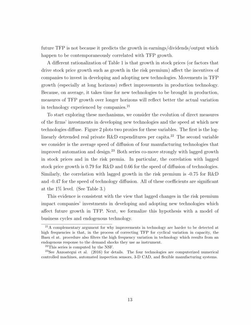
To start exploring these mechanisms, we consider the evolution of direct measures
of the firms’ investments in developing new technologies and the speed at which new
technologies diffuse. Figure 2 plots two proxies for these variables. The first is the log-
linearly detrended real private R&D expenditures per capita.22 The second variable
we consider is the average speed of diffusion of four manufacturing technologies that
improved automation and design.23 Both series co-move strongly with lagged growth
in stock prices and in the risk premia. In particular, the correlation with lagged
stock price growth is 0.79 for R&D and 0.66 for the speed of diffusion of technologies.
Similarly, the correlation with lagged growth in the risk premium is -0.75 for R&D
and -0.47 for the speed of technology diffusion. All of these coefficients are significant
at the 1% level. (See Table 3.)
This evidence is consistent with the view that lagged changes in the risk premium
impact companies’ investments in developing and adopting new technologies which
affect future growth in TFP. Next, we formalize this hypothesis with a model of
business cycles and endogenous technology.
21A complementary argument for why improvements in technology are harder to be detected athigh frequencies is that, in the process of correcting TFP for cyclical variation in capacity, theBasu el at. procedure also filters the high frequency variation in technology which results from anendogenous response to the demand shocks they use as instrument.
22This series is computed by the NSF.23See Anzoategui et al. (2016) for details. The four technologies are computerized numerical
controlled machines, automated inspection sensors, 3-D CAD, and flexible manufacturing systems.
13

Table 3: Stock Prices and Endogenous Technology Correlation
Private R&D Speed of Technology Diffusion
Stockt−20,t 0.79*** 0.66***
Premiumt−13,t−1 -0.75*** -0.47**
Note: (i) Stock is the value of the stock and bonds of the companies in the S&P 500deflated by the GDP deflator; (ii) Stockt−20,t is the annualized growth rate in thestock market past five years; (iii) Premiumt−13,t−1 is the annualized growth rate inrisk premium past three years; (iv) Private R&D is the the log-linearly detrendedreal private R&D expenditures per capita, which is computed by the NSF; (v)Speed of Technology Diffusion is the average speed of diffusion of four manufacturingtechnologies that improved automation and design. See Anzoategui et al. (2015)for details. The four technologies are computerized numerical controlled machines,automated inspection sensors, 3-D CAD, and flexible manufacturing systems.
3 Model
Our model is a one-sector, real business cycle model extended to allow for endogenous
development and adoption of new technologies and for exogenous fluctuations in risk
premia. We introduce a (time-varying) risk-premium by assuming that consumers
dislike holding stocks and their aversion to stocks fluctuates stochastically. We endo-
genize technology by allowing agents to engage in research activities that result in the
development of new intermediate goods. Invented, intermediate goods are adopted
at an endogenous rate leading to higher total factor productivity. For simplicity, we
abstract from many other mechanisms that are standard in business cycle and asset
pricing models but that are not critical to explore our hypothesis on the co-movemnet
between stock prices and future TFP growth.
3.1 Consumers
Consumers consume, supply labor and decide how to allocate their wealth. Each
consumers supplies two types of labor: skilled, Lst, and unskilled, Lut. The former is
used in R&D and technology adoption activities, while the latter is used in produc-
14

tion.24 Agents hold two types of securities: risk-free bonds, Bt, that are in zero net
supply, and claims to the portfolio composed by all the companies in the economy
(i.e. the market portfolio). Each claim has a price of 1. So, the value of the claims
held by the representative consumer is equal to the number of claims they demand,
Qdt . Let Rf
t denote the gross return on risk-free bonds and Rt the gross return on a
claim to the stock market. To introduce a risk premium, we assume that consumers
derive disutility from holding claims to the market portfolio. In particular the flow
of utility is
ut = log(Ct − ψhCt−1)−
[µw
L1+ϕuut
1 + ϕu+ µs
L1+ϕsst
1 + ϕs
]− ζtQd
t , (3)
where ζt captures the stochastic disutility from holding stocks, µw is the disutility
from supplying unskilled labor and µs is the disutility from supplying skilled labor.
The representative consumer maximizes the present discounted flow of utility given
by equation (4), subject to the budget constraint (5) and a No-Ponzi game condition.
Max{Ct+i, Lt+i, Lst+i, Bt+i, Qdt+i}∞i=0
Et
∞∑i=0
βi {ut+i} (4)
Bt+i+1 +Qdt+i+1 + Ct+i + Tt+i =
∑v∈{u,s}
W vt+iLvt+i +Rf
t+iBt+i +Rt+iQdt+i (5)
The first order conditions that characterize the solution to the consumers problem
are:
υtWut = µwL
ϕuut (6)
υtWst = µsL
ϕsst (7)
Et
[βΛt,t+1R
ft+1
]= 1 (8)
Et[βΛt,t+1
(Rt+1 − ψt+1
)]= 1 (9)
24For the time being we treat workers as homogeneous. When estimating the model we introducewage rigidities as in Erceg et al. (2000). This variation requires assuming that labor is differentiated,see the appendix for more details.
15

where the stochastic discount factor, Λt,t+1, is given by
Λt,t+1 =υt+1
υt(10)
υt =1
Ct − ψhCt−1
− β ∗ ψhCt+1 − ψhCt
(11)
and
ψt+1 = ζt+1 ∗ υt+1
Combining equations (8) and (9), we obtain the following expression for the risk
premium (Rt−Rft ) in which it is clear that, to a first order, the risk premium is equal
to ψt+1.
Et
[βΛt,t+1
(Rt+1 −Rf
t+1
)]= Et
[βΛt,t+1ψt+1
](12)
3.2 Production
There is a continuum At of intermediate goods available for production. Each interme-
diate good is produced by one producer with the following Cobb-Douglas production
function:
Yit = χtKαit (Luit)
1−α , (13)
where Yit denotes the amount of the ith intermediate good produced, χt is an aggregate
productivity shock, Kit is the capital rented by the ith producer, and Luit the amount
of unskilled labor hired.
Let ηit be the marginal cost of production of the ith intermediate good producer,
W ut the unskilled wage rate, DK
t the rental rate of capital net of depreciation, δ the
depreciation rate and PKt the cost of replacing one unit of capital. Cost minimization
implies:
ηitαYitKit
= [DKt + δPK
t ] (14)
ηit(1− α)YitLuit
= W ut (15)
Intermediate goods are bought by a competitive firm that combines them to produce
16

aggregate output as follows:
Yt =
(∫ At
0
Y1/ϑit di
)ϑ, ϑ > 1. (16)
Normalizing the price of aggregate output to 1, we can express the demand faced by
a intermediate good producer as
Yit = Yt (Pit)− ϑϑ−1 . (17)
Given this demand function, if intermediate producers were unconstrained, the prices
would be a constant gross markup, ϑ, times the marginal cost of production, ηit..
Following Jones and Williams (2000) and Aghion and Howitt (1997), we disentangle
markups from the elasticity of substitution among intermediate goods by recognizing
that the threat of imitation by competitors may limit the mark up they can charge
to µ. The equilibrium markup charged by intermediate goods producers , µ, is then
given by
µ = min {ϑ, µ} . (18)
This yields the following expression for the profits of an intermediate good producer
πt = (µ− 1)ηitYit (19)
Using the normalization of the price of output, the demand functions, pricing rules
for intermediate and the intermediate production functions, we can derive expressions
for the aggregate production function, aggregate factor demands and profit flows in
the symmetric equilibrium. In particular, aggregate output is equal to
Yt = θtKαt (Lut )
1−α (20)
where Kt =∫ At
0Kitdi is the aggregate capital stock, Lut =
∫ At0Luitdi is the number
of unskilled hours employed in the economy and θt is the TFP level. As shown in
equation (21) TFP has two components. The exogenous aggregate shock, χt, and the
17

endogenous productivity gains associated with the adoption of new technologies, At.
θt = χtAϑ−1t (21)
The aggregate demands for capital and labor are
αYtKt
= µ[DKt + δPK
t+1] (22)
(1− α)YtLut
= µW ut . (23)
And the equilibrium profit flows for the representative producer of an adopted
intermediate good are
πt =(µ− 1)YtµAt
. (24)
3.3 Capital producers
Capital is produced competitively by transforming final output into new investment.
In particular, it takes one unit of output to produce one unit of capital. As in
Gertler and Karadi (2011), we assume that the production of net investment is subject
to flow adjustment costs. Specifically, capital goods producers solve the following
maximization problem:
max{Int+τ}
Et
∞∑τ=0
Λt,τ
{(P I
t+τ − 1)Int+τ − f(
Int+τ + It+τγy(Int+τ−1 + It+τ−1)
)(Int+τ + It+τ )
}
where P It+τ denotes the price of installed capital, It is the steady state level of
(gross) investment in period t, γy is the gross growth rate of output in the steady
state, and Int is net investment:
Int = It − δKt (25)
Furthermore, we assume that f(1) = f ′(1) = 0, and f ′′(1) > 0.
Optimal production of investment is given by the following condition:
18

P It = 1 + f (.) +
Int + Itγy(Int−1 + It−1)
f ′(.)− Et
[Λt,t+1
(Int+1 + It+1
γy(Int+ + It)
)2
f ′(.)
](26)
The law of motion for the capital stock in the economy is
Kt+1 = Kt + Int. (27)
3.4 Technology
Technology is not manna from Heaven. Agents invest resources to develop and adopt
new technologies that enhance the productive possibilities of the economy (At). Tech-
nology diffusion and development are not instantaneous processes. As in Comin and
Gertler (2006), we capture the slow diffusion of technology by introducing two se-
quential investments. Agents first develop new prototypes through R&D. Then they
engage in stochastic investments that, if successful, make the resulting intermediate
good usable for production. The stochastic nature of this second investment implies
that, on average, there is a lag between the time of invention of the technology and
the time in which it is used in production.
Formally, individual researchers perceive that a unit of skilled labor produces κt
new technologies, where
κt =κZt
S1−ρt
. (28)
κ pins down the productivity of R&D activities, St is total amount of research services
employed in the economy, Zt is the stock of all intermediate goods developed and
ρ ∈ (0, 1) . This formulation captures diminishing returns to aggregate R&D, and
knowledge spillovers that ensure the existence of a balanced growth path.
A fraction (1 − φ) of developed technologies becomes obsolete every period. The
resulting law of motion for the technologies developed by researcher p, Zpt , is:
Zpt+1 = φκtS
pt + φZp
t (29)
Aggregating equation (29) among all researchers, we obtain the following law of
19

motion for the stock of technologies is:
Zt+1 = (φκSρt + φ)Zt. (30)
Before being used in production, intermediate goods need to be adopted. Potential
adoption firms competitively bid for the right to adopt each intermediate good. After
gaining the right to adopt an intermediate good, an adoption firm, hires ht hours of
skilled labor to face a probability λt that the prototype is usable for production at
time t+ 1. In particular,
λt = λ(Ztht) (31)
with λ′ > 0, λ′′ < 0.25 This formulation assumes that past experience with technology,
measured by the total number of intermediate goods developed Zt, facilitates the
adoption of new technologies. This assumption ensures the existence of a balanced
growth path where the speed of adoption is λ, and the average delay between the
development and adoption of technologies (i.e., the adoption lag) is 1/λ.
The law of motion for the aggregate number of adopted intermediate goods in the
symmetric equilibrium is:
At+1 = φAt + φλt(Zt − At). (32)
The adoption and R&D intensities are driven by the value of adopted and un-
adopted intermediate goods. The value of an adopted intermediate good, vt, is given
by the present value of profits from commercializing the technology. Formally, vt is
defined recursively by the Bellman equation
vt = πt + Et [φvt+1/Rt+1] , (33)
where 1/Rt+1 is the discount factor applied by intermediate good producers between
t and t+ 1.
Adopters are willing to bid for prototypes up to the value of the option to adopt
25In particular, we assume thatλ(Z ∗ h) = λ(Zh)ζ
20

them, jt, which is given by
jt = maxht−W s
t ∗ ht + Et{φ[λtvt+1 + (1− λt)jt+1]/Rt+1}, (34)
where W st is the wage rate of skilled labor.
Free entry into R&D implies that the discounted value of intermediate goods cre-
ated every period equals the cost of skilled labor engaged in R&D (35).
W st St = Et
[R−1t+1(Zt+1 − Zt)jt+1
]. (35)
Optimal investment in adopting a new technology requires that the marginal cost
of adoption services equals their expected marginal benefit (36).
W st = Et
[R−1t+1Ztφλ
′ (Ztht) (vt+1 − jt+1)]
(36)
A market clearing condition ensures that the supply of research labor equals its
demand for R&D and adoption activities.
Lst = St + ht ∗ (Zt − At) (37)
Equations (35) and (36) illustrate the cyclical properties of aggregate R&D and
adoption expenditures. In general, there are two sources of cyclicality. On the one
hand, the pro-cyclicality of profits accrued by intermediate goods producers (19)
makes both the value of unadopted goods (jt+1) and the capital gains from adoption
(vt+1 − jt+1) pro-cyclical. On the other, the cyclicality of the research wage rate
makes the cost of R&D and adoption pro-cyclical. These two forces have opposing
effects on the cyclicality of R&D and adoption. The first force tends to make them
pro-cyclial while the second tends to make them counter-cyclical. Thus, in principle,
the sign of the co-movement between output and adoption and R&D investments is
ambiguous.26 Empirically, however, wages are significantly less pro-cyclical that what
26The literature on endogenous growth has struggled to reconcile the labor intensity of R&D withthe pro-cyclicality of R&D investments (see, e.g., Aghion and Saint-Paul (1994), Aghion and Howitt(1992). Other approaches to reconcile these two facts are to introduce financial frictions (Aghionet al. (2011) and short term biases of innovators (Barlevy (2007)). To the best of our knowledge,the first model that resorted to wage rigidities to produce pro-cyclical R&D in a setting with laborintensive R&D was Anzoategui et al. (2015).
21

the flexible wage model predicts. To match the cyclicality of wages, we will introduce
wage rigidities when we estimate the model. Once we have a realistic wage profile,
the pro-cyclicality of the value of unadopted technologies and the capital gains from
adoption dominates leading to pro-cyclical adoption and R&D investments as we shall
see below.
In addition to these two channels, risk premium shocks affect the R&D and adop-
tion decisions through two additional ones. For a given flow of profits, risk premium
shocks affect the rate at which future profits are discounted and hence the value of
adopted and unadopted technologies (See equations 33 and 34). Furthermore, for a
given jt+1 and on (vt+1 − jt+1), risk premium shocks affect the return required by
researchers and adopters from their investments. (See equations 35 and 36.) These
two forces strengthen the cyclicality of R&D and adoption when the economy is hit
by risk premium shocks.27
3.5 The value of corporations
The market value corporations, Qt, reflects the value of all their assets. This includes
physical assets such as capital, as well as intangible assets such as the right to produce
adopted intermediate goods and the option to adopt developed intermediate goods.
Formally,
Qt =
Value of installed capital︷ ︸︸ ︷P It Kt +
Value of adopted technologies︷ ︸︸ ︷At(vt − πt) +
Value of unadopted technologies︷ ︸︸ ︷(Zt − At)(jt + ht ∗W s
t ) (38)
It is important to note that the stock market value is quite different in our model
from standard macro models. In models where technology is exogenous, the only
asset corporations own is their physical capital. Therefore, the stock market value is
just given by the first term in equation (38). In contrast, in our model, stock prices
are affected by factors that impact the stream of profits from commercializing new
technologies (and the rates at which those are discounted). In addition to providing
a richer theory of stock price fluctuations, recognizing the market value of technology
allows us to account for the significant wedge that exists between stock prices and
27Indeed, these investments are always pro-cyclical with risk premium shocks even in the absenceof wage rigidities as we shall see below.
22

the book value of capital (see, e.g., Hall (2001), McGrattan and Prescott (2001)).
Another feature of equation (38) that is worth noting is that Qt does not include
the value of technologies that have not been developed yet. This is the case because
the arrival of intermediate goods in the future is not a free lunch. The free entry
condition (35), implies that, in equilibrium, the expected present discounted value
of profits accrued by the producers of future intermediate goods equals the cost of
developing them. Therefore, their net value is zero.28
We can also compute the aggregate dividends distributed in the economy, Dt as
Dt =
Rental of K︷ ︸︸ ︷DKt Kt +
Profits from A︷︸︸︷Atπt −
Adoption costs︷ ︸︸ ︷(Zt − At) ∗ ht ∗W s
t (39)
Akin to the expression for stock prices, dividends have three components. The
first is the revenues from renting capital. The second corresponds to the operating
profits from commercializing intermediate goods. The third, are the costs of adopting
intermediate goods.
Without loss of generality, we assume that the price of a claim on the stock market
is equal to one. Therefore, the number of claims held by the households, Qdt , is equal
to the stock market value, Qt.
Qdt = Qt (40)
The realized return from holding stocks is then given by:
Rt =Dt +Qt
Qt−1
(41)
3.6 Government
To match the model production structure to the National Income and Product Ac-
counts we introduce a passive government that finances an exogenous expenditure
flow, Gt, with lump sum taxes, Tt, levied on households. We assume that the govern-
28Conversely, if new technologies arrive exogenously as in Comin et al. (2009) and Iraola andSantos (2007), the expression for the stock market has an additional term that captures the valueof all technologies that will arrive in the future to the economy.
23

ment runs a balanced budget every period:
Gt = Tt (42)
3.7 Equilibrium
The economy has a symmetric sequence of markets equilibrium. The equilibrium is
characterized by the following conditions:
1. Consumers optimally supply both types of labor and determine their consump-
tion and portfolio allocation as described in equations (6-9).
2. Intermediate goods producers demand capital and labor optimally according to
equations (22) and (23), and charge a markup given by (18).
3. Investment in physical capital satisfies the optimality condition (26).
4. R&D expenditures satisfy the free entry condition (35).
5. Adoption expenditures maximize the expected value of adopters by satisfying
equation (36).
6. The endogenous state variables, Kt, Zt and At evolve according to equations
(27), (30) and (32).
7. The resource constraint of the economy is:
Yt = Ct +Gt + It
8. The markets for skilled (37) and unskilled labor (equations 23 and 6) clear.
9. The market for claims on stocks clears (40).
4 Empirical evaluation
We next evaluate the model’s ability to produce the predictability patterns unocov-
ered in section 2. To this end, we conduct two types of exercises. The first uses data
24

simulated from the model after calibrating the volatility of risk premium and exoge-
nous TFP shocks to their empirical volatilities. The second uses the historical series
of TFP and risk premium to identify the model-consistent shocks series. With the
simulated data we evaluate the model’s ability to produce the predictability of TFP
growth observed in the data. The historical analysis of the sources of predictability
provides further evidence to identify our mechanisms from others. In particular, it
allows to explore whether stock prices and risk premia growth predict the historical
endogenous or exogenous components of TFP growth. Before presenting these exer-
cises, we describe the model calibration and present its impulse response functions
and theoretical moments.
4.1 Calibration
Table 4 presents the calibrated parameters and their values. There are four types
of parameters. Those that parameterize (i) the preferences, (ii) the production and
markups, (iii) the endogenous technology mechanisms, and (iv) the shocks. Since
first two types of parameters are fairly standard in the literature, we postpone the
dicussion of their calibration to the Appendix. Here we mostly focus on explaining
the calibration for the endogenous technology parameters and the processes followed
by the shocks.
Five parameters pin down the endogenous technology mechanisms. The value of
κ is set to match the long-run growth rate of the economy which we assume it to
be 2% per year. The elasticity of the number of intermediate goods with respect to
R&D labor, ρ, is set to 0.35 following the estimates of Anzoategui et al. (2015).29
λ is set to produce an average adoption lag of 7 years which is consistent with the
estimates in Comin and Hobjin (2010) and Cox and Alm (1996). The elasticity of λ
with respect to adoption efforts, ζ, is set to 0.85 to induce a ratio of private R&D to
GDP consistent with the U.S. post-1970 experience (of approximately 1.5% of GDP).
Finally, the obsolescence rate (1 − φ) is set to 4% annual following the estimate of
Caballero and Jaffe (1993). Section 4.7 conducts a robustness analysis to alternative
calibrations of the values of ρ and ζ.
29Unlike the rest of the literature, this paper estimates the curvature of R&D in the context ofa quarterly model like ours. Because of greater diminishing returns in R&D at the high frequency,the point estimate of ρ is lower than in the rest of the literature (e.g., Griliches, 1990).
25

Table 4: Calibrated parameters
Parameter Description Value
Preferencesβ Discount factor 0.995ψh Habit formation 0.7ϕs Inverse labor supply elasticity for skilled workers 0.5ϕu Inverse labor supply elasticity for unskilled workers 0.5ψ Steady state risk premium 0.07/4
Production/markupα Share of capital in GDP 0.33δ Depreciation rate 0.02f ′′(1) Investment adjustment cost parameter 3ϑ Gross markup for differentiated intermediate goods 1.5µ Constrained gross markup 1.25G/Y Government spending-output ratio 0.16
Endogenous technologyκ The average productivity of R&D, set to match the steady
state growth rate of 2% per yearλ Set to produce the average adoption rate of 0.15 annuallyρ Elasticity of succesfully developing a new tech
wrt the stock of developed intermediate goods 0.35ζ Elasticity of adoption 0.85φ Survival probability for intermediate goods 0.99
Shocksσ2ψ Variance of risk premium shocks 0.1582
σ2χ Variance of exogenous TFP shocks 0.812
ρψ Persistence of risk premium shocks 0.987ρχ Persistence of exogenous TFP shocks 0.92
26

There are two parameters that measure markups and elasticities of substitution.
We set the elasticity of substitution between intermediate goods to 3 so that the
unconstrained gross markup ϑ is 1.5, which is consistent with the estimates of Broda
and Weinstein (2010). We set the constrained gross markup charged by intermediate
goods producers, µ, to 1.25 as suggested by the estimates of Norrbin (1993) and Basu
and Fernald (1997). This calibration yields a share of physical capital value in the
total stock market value of 45% which virtually coincides with the average for the
S&P 500 over our sample period of 42%.30 The value of adopted technologies account
for 52% of stock prices in steady state, while unadopted technologies account for the
remaining 3%.
In our model we restrict exogenous disturbances to only the risk premium and the
exogenous TFP shocks. With this strategy we do not intend to disregard the relevance
of other shocks but rather to focus on the minimal set of shocks that allows us to
study meaningfully the co-movement between stock prices and TFP. This perspective
also guides our approach to calibrate the volatility and persistence of our two shocks.
We set the standard deviation and autocorrelation of the risk premium shock to
match those of the proxy we have built by forecasting the ex-post excess return by
the lagged log-price-dividend ratio (See section 2). To calibrate the parameters in
the exogenous TFP process, we first identify the actual realizations of this shock
necessary to generate the TFP growth series (1970:I - 2008:III) from Fernald (2014)
with our model. Then we set the autocorrelation of exogenous TFP (χt) and the
standard deviation of its innovations to match those in the identified exogenous TFP
series.
4.2 Impulse response functions
To gain a better understanding of the workings of our model, we next study its impulse
response functions. Figure 3 plots the impulse response functions to a one standard
deviation positive shock to the risk premium. For comparison purposes, we also plot
(in dashed red) the response of a version of the model with the same parameter values
but without adoption and R&D (i.e. with exogenous technology).
30Note that, counter-factually, the value of installed capital fully accounts for stock prices instandard macro models with exogenous technology.
27

0 5 10 15 20 25 30 35 40-2.5
-2
-1.5
-1
-0.5
01. Output
Endogenous TechnologyExogenous Technology
0 10 20 30 40-0.8
-0.6
-0.4
-0.2
02. Unskilled hours
0 10 20 30 40-1.5
-1
-0.5
0
0.53. Consumption
0 5 10 15 20 25 30 35 40-10
-8
-6
-4
-2
04. Investment
0 10 20 30 40-3.5
-3
-2.5
-2
-1.5
-15. Value of installed capital
0 10 20 30 40-7
-6
-5
-4
-3
-26. Value of technologies
Unadopted technologiesAdopted technologies
Period0 5 10 15 20 25 30 35 40
-3.5
-3
-2.5
-2
-1.5
-17. Stock market
0 10 20 30 40-7
-6
-5
-4
-3
-2
-18. λ and S
λ: speed of diffusionS: R&D
Period0 10 20 30 40
-0.8
-0.6
-0.4
-0.2
0
0.29. Endogenous TFP
Period0 10 20 30 40
0.08
0.1
0.12
0.14
0.1610. Risk premium shock
Figure 3: Impulse Response Functions to a Risk Premium Shock
The risk premium shock raises the rate of return required to invest in physical
capital causing a decline in investment. Consumption, instead, increases slightly. As
a result, the risk premium shock causes an initial decline in output.
The higher premium causes an immediate drop in the value of adopted and un-
adopted technologies (see panel 6). Potential adopters and intermediate good devel-
opers respond to this decline in the value of technologies by cutting the number of
skilled hours devoted to R&D and adoption. Hence, the large drop in S and λ (see
panel 8). The slowdown in R&D and adoption causes a gradual decline (relative to
trend) in the number of adopted intermediate goods, and hence in the endogenous
component of TFP (i.e., At∗(ϑ−1)). This protracted effect is mirowed by output (and
28

capital). Forty quarters after the shock, output has dropped by almost 3 percentage
points and the endogenous component of TFP has declined by almost 1 percentage
point.
In the short term, output evolves very similarly in the endogenous and exogenous
technology models sugegsting that the endogenous technology mechanisms do not
produce much amplification of business cycle shocks. Over time, our model produces
a significantly larger drop in output. Note that the response of investment is very
similar in the endogenous and exogenous technology models throughout. Therefore,
the gap in output is driven by the effect of the premium shock on the stock of adopted
technologies.
Stock prices drop by almost three percentage points upon the increase in the
risk premium (by one standard deviation). This drop is nearly 50% larger than
in the model with exogenous technology. This wedge reflects the different notions
of the stock market in both models. While stock prices just reflect the value of
installed capital in the exogenous technology model, once technology is endogenized,
the value of corporations also includes the value of the technology they develop and
adopt. Because the risk premium affects more the values of adopted and unadopted
technologies than the installed price of capital (see panels 5 and 6), stock prices drop
more in the endogenous technology model. The gradual drop in the stock of adopted
and developed technologies, together with the decline in the capital stock, lead to a
subsequent decline in stock prices which level of at around 4%.
The evolution of stock prices in our model contrast with that in Pastor and Veronesi
(2009). In their model, once a revolutionary technology reaches a certain diffusion
level, it moves from being an idiosyncratic to being an aggregate risk causing a collapse
in stock prices. In our model, instead, the risk premium shock contemporaneously
impacts the diffusion rate pro-cyclically. This co-negative movement pattern between
risk premia and speed of technology diffusion is consistent with the evidence presented
in section 2.
The response of the speed of technology diffusion and R&D to the premium shock
cause a pro-cyclical evolution in the growth rate of TFP which results in a perma-
nent shift in the level of TFP. These dynamics are consistent with the predictability
patterns documented in section 2.
Figure 4 plots the impulse response function to one standard deviation increase
29

0 10 20 30 400.1
0.2
0.3
0.4
0.5
0.6
0.71. Output
Endogenous TechnologyExogenous Technology
0 10 20 30 40-0.4
-0.3
-0.2
-0.1
0
0.12. Unskilled hours
0 10 20 30 400
0.2
0.4
0.6
0.8
13. Consumption
0 10 20 30 400
0.5
1
1.54. Investment
0 10 20 30 400.2
0.4
0.6
0.8
15. Value of installed capital
0 10 20 30 400
0.5
1
1.56. Value of technologies
Unadopted technologiesAdopted technologies
Period0 10 20 30 40
0
0.5
1
1.57. Stock market
0 10 20 30 40-0.04
-0.02
0
0.02
0.04
0.068. λ and S
λ: speed of diffusionS: R&D
Period0 10 20 30 40
×10-3
-1
0
1
2
3
49. Endogenous TFP
Period0 10 20 30 40
0
0.2
0.4
0.6
0.8
110. Exogenous TFP shock
Figure 4: Impulse Response Functions to a TFP Shock
30

in exogenous TFP. The higher productivity immediately raises output, consumption
and investment. Hours worked decline because the income effect dominates the sub-
stitution.31 Stock prices increase reflecting the greater value of installed capital and
of newly developed and adopted technologies. The greater value of technologies tends
to induce greater investments in adoption and R&D. These are partially mitigated by
the increase in the wage for skilled workers. Upon impact, the value effect dominates
the wage effect for R&D. For adoption they nearly cancel out. As a result the number
of adopted technologies does not increase initially. Slowly the effect on the value of
adopted technologies dominates the increase in skilled wages, leading to a gradual
increase in the number of adopted technologies and in the endogenous component
of TFP. This effect is considerable smaller than the effect induced by the premium
shock.
Figure 4 also illustrates the inconsistency of exogenous TFP with the predictability
patterns uncovered in section 2. As mentioned above, stock prices increase upon
impact of a positive TFP shock. After that moment, the mean reversion of the shock
leads to a decline in TFP that the endogenous TFP component cannot mitigate.
Therefore, exogenous TFP shocks cause a negative predictability of lagged stock price
growth on future TFP growth. Furthermore, because in our model risk premia are
exogenous, TFP shocks do not play any role in the predictability reported in Table
(1) of risk premia on future TFP growth.
4.3 Theoretical moments
Before evaluating the predictability of TFP growth in the model, we explore the
theoretical moments it produces (see Table 5).32 Columns 1 and 2 report the standard
deviation of variables relative to the standard deviation of output (in the model and
the data).33 The relative volatility of stock prices, dividends and the speed of adoption
31This is the case because of the habit and the higher persistence induced by the endogenoustechnology mechanisms. The effect of TFP shocks on hours worked is consistent with teh VARevidence from Gali (1999).
32All variables are HP filtered.33We try to preserve the simplicity of our model by limiting the number of shocks and propagation
mechanisms. The standard deviation of HP-filtered output in the model is 0.8 while in the data itis 1.55.
31

is in the ballpark of the data.34 The most significant deviation from the data is that
the model greatly overpredicts the volatility of R&D expenditures.35 This surely
reflects the lack of adjustment costs in the R&D employment decision in the model.
In reality, the volatility of R&D expenditures is lower than what our model predict
due to the presence of planning costs and labor hoarding.36 In section 4.6, we present
evidence that suggests that the excess volatility of R&D in the model is not key for
the predictability of TFP.
Table 5: Theoretical moments
Variable Standard deviation Autocorrelation Variance DecomposisionData Model Data Model Risk premium TFP
Y 1 1 0.83 0.90 31.84 68.16(0.73, 0.92)
St 4.92 4.15 0.77 0.63 77.64 22.36(0.66, 0.89)
Dt 1.74 2.83 0.94 0.69 85.71 14.29(0.87 , 1)
Adoption rate* 5.68 4.02 -0.46 0.16 99.89 0.11(-0.78, -0.14)
RD expenditure* 3.05 9.60 0.91 0.14 99.99 0.01(.74, 1.08)
Note: All variables are HP filtered. Standard deviations are relative to output.* Annual Data
The autocorrelation and cyclicality of the variables is roughly in line with the
data. The main deviation is the speed of adoption which in our series appears mean
34The discrepancy in the relative volatility of dividends is magnified by the measures of dividendsused in the data and in the model. The empirical measure of dividends is real quarterly S&Pdividends per capita from Shiller. An alternative measure of profitability is earnings which aresignificantly more volatile than dividends.
The reported dividend measure in the model is given by equation (39) and is net of adoption costs.If adoption costs are not netted, the relative volatility of dividends in the model is 1.31. In reality,we do not know how much of the costs of adopting new technologies are passed to shareholders inthe form of lower dividends. But it is reassuring that the empirical volatility of dividends falls withinthe model volatilities in the two polar cases.
35We compute R&D expenditures as R&D labor times the skilled wage rate (i.e., St ∗WSt ).
36The greater volatility of non-labor than labor costs in R&D suggests the prevalence of laborhoarding in R&D.
32

reverting at the high frequency due to the small sample of technologies we use to
construct it.
Columns 7 and 8 of Table 5 decompose the variance of the HP-filtered variable
between the contribution of risk premium and TFP shocks. TFP shocks account for
approximately twice as much variance of output as risk premium shocks. For the rest
of the variables, the risk premium shock accounts for a much greater variance than
the TFP shock. In particular, the variance share attributable to risk premium shocks
are 78% for stock prices,37′38 88% for dividends, 100% for the adoption rate and
97% for R&D expenditures. The importance of risk premium shocks in the volatility
of adoption and R&D is a consequence of the dual effect of the risk premium on
the marginal benefit from developing and adopting a technology. While the effect
of standard macro shocks is mostly operating through their impact on the profit
flows, risk premium shocks have an additional effect through the rate at which these
profit flows are discounted. This second effect makes risk premia a powerful driver of
fluctuations in the technology upgrading margins.
4.4 Predictability
We can now proceed to evaluate the model’s ability to account for the predictability
of future TFP growth with lagged stock price growth uncovered in the data. To this
end, we simulate 10,000 times the model and, for each one, we run the predictability
regressions (1).39
37This finding is consistent with the estimates in Campbell and Shiller (1988a).38For comparison purposes, we have conducted a similar decomposition in a version of our model
with the same parameter values and shocks but without the endogenous technology mechanisms.The risk premium shock accounts for 57% of the stock market variance.
39Each run is 556 periods long, and we discard the first 400 periods before running the regressions.
33

Tab
le6:
PredictabilityofTFP
withStock
Pricesand
Risk
Premia:Modelvs.
Data
Dep
enden
tIn
dep
enden
tH
oriz
on(p
)va
riab
leva
riab
le5
1015
2025
3035
40TFPt,t+p
Stock
t−20,t
Dat
a0.
033
0.04
80.
046
0.05
1∗0.
054∗∗∗
0.04
9∗∗∗
0.04
6∗∗∗
0.04
2∗∗∗
s.e.
0.03
40.
0316
0.02
940.
0271
0.02
470.
0226
0.02
080.
0192
R2
0.02
0.11
0.15
0.21
0.28
0.28
0.28
0.26
Model
0.05
70.
055
0.05
20.
047
0.04
10.
035
0.02
80.
022
R2
0.09
40.
182
0.25
70.
321
0.37
30.
418
0.45
80.
495
Exog
enou
sT
echnol
ogy
Model
-0.0
94-0
.078
-0.0
65-0
.054
-0.0
46-0
.040
-0.0
35-0
.032
R2
0.03
00.
057
0.08
40.
112
0.13
90.
167
0.19
50.
223
TFPt,t+p
Premiumt−
13,t−
1D
ata
-0.5
4-0
.58−
0.64∗∗−
0.58∗∗∗−
0.48∗∗−
0.41∗−
0.32∗
-0.1
9s.
e.0.
390.
350.
310.
270.
240.
220.
200.
19R
20.
060.
160.
280.
290.
270.
280.
230.
1
Model
-0.8
94-0
.830
-0.7
77-0
.724
-0.6
68-0
.608
-0.5
46-0
.484
R2
0.09
0.18
0.25
0.30
0.35
0.39
0.43
0.47
Exog
enou
sT
echnol
ogy
Model
0.03
90.
036
0.02
30.
012
0.00
3-0
.001
-0.0
010.
002
R2
0.02
80.
053
0.06
90.
082
0.09
40.
108
0.12
40.
140
Not
e:(i
)Sta
ndar
der
rors
(s.e
.)ar
eco
mpute
dby
aM
onte
Car
lopro
cedure
asex
pla
ined
inth
ete
xt.R
2is
the
R-s
quar
edfr
omth
ere
gres
sion
.P
erio
dis
1947
-201
3fo
rSto
ckpri
ces
and
1970
-201
3fo
rri
skpre
miu
m;
(ii)
TF
Pis
corr
ecte
dfr
omva
riat
ion
inca
pit
aluti
liza
tion
,in
crea
sing
retu
rns
and
imp
erfe
ctco
mp
etit
ion
asin
Bas
uet
al.
(200
6);
(iii)
Sto
ckis
the
valu
eof
the
stock
and
bon
ds
ofth
eco
mpan
ies
inth
eS&
P50
0defl
ated
by
the
GD
Pdefl
ator
;(i
v)TFPt,t+p
isth
eav
erag
egr
owth
rate
ofT
FP
bet
wee
nquar
ters
tan
dt+
p;
(v)Stock
t−20,t
isth
ean
nual
grow
thra
tein
the
stock
mar
ket
bet
wee
nquar
ters
t-20
and
t;(v
i)TFPt+p
islinea
rly
det
rended
TF
P.
***
den
otes
sign
ifica
nt
atth
e1%
leve
l,**
atth
e5%
leve
l,an
d*
atth
e10
%le
vel.
34

Table 6 reports the average point estimates of the predictability regressions in the
simulated data and compares them with those in the actual data. 40 The top panel
uses lagged growth in stock prices over the last 5 years as forecasting variable. Our
main finding is that the predictability of TFP growth by lagged stock price growth
in the model is very similar to what we have found in the data. For example, the
coefficient of lagged stock price growth (over five years) on future TFP growth over a
20 quarter horizon is 0.047 in the model and 0.051 in the data. When increasing the
TFP horizon to 35 quarters the model’s estimate is 0.028 while the data counterpart
is 0.046. Over short horizons, the model produces higher estimates than the data
although the difference is not statistically significant. In terms of predictive power,
the model matches the high predictability observed in the data of lagged growth in
both stock rices and risk premia on future TFP growth.
The bottom panel of Table 6 uses the growth in the risk premium over the previous
three years as forecasting variable. We find that in the model the lagged premium
growth also predicts future TFP growth. In particular, both the average coefficient
and predictive power from the simulated data are in line with the data. For example,
at a 20 quarter horizon, the coefficient of lagged premium growth on future TFP
growth is -0.58 in the actual data vs. -0.72 in the model-simulated data. The respec-
tive R2s are 0.29 vs. 0.3.41 We conclude from these exercises that our model accounts
quantitatively for the predictability of TFP growth documented in section 2.
For comparison purposes, we study the predictability of TFP in a version of our
model with exogenous technology.42 This exercise allows us to evaluate whether ex-
ogenous TFP shocks in a q-theory model of investment can produce the co-movement
patterns between stock prices and TFP growth documented in the data.
One immediate limitation of neoclassical investment models is that they cannot
produce any TFP growth predictability with risk premia. This follows from the
fact that, in q-theory models, both TFP and risk premia are exogenous independent
processes that, by construction are independent. Therefore in the simulated data
40Given the sample size, the precision of the average point estimate is very high (and we do notreport it).
41All estimates are statistically significant.42The model parameters and shocks processes are set to the same values as in the estimated
endogenous technology model.
35

there will be no co-movement between TFP growth and risk premia.43
Accordingly, we focus on the power of the exogenous technology model to produce
the TFP-growth predictability with lagged stock price growth over the past 5 years as
predicting variable. The sixth row in Table 6 presents the average point estimates. In
contrast to the empirical evidence, in the simulations from the exogenous technology
model, lagged stock price growth is associated with lower future TFP growth. The
intuition behind this result is as follows. A positive TFP shock leads to higher
future dividends and, therefore, to higher stock prices. Because TFP shocks are mean
reverting, an increase in stock prices triggered by a positive TFP shock is associated
with negative TFP growth in the future. Hence the impossibility of the exogenous
technology model to account for the empirical predictability of future TFP growth.
Another way to interpret the estimates in Table 6 are in terms of the sources of
TFP growth that cause the predictability. Equation (21) implies that TFP can be
decomposed between endogenous and exogenous components. This decomposition
motivates the question of which of the two components is actually predictable by lag
growth in stock prices and risk premium. To answer this question, we can compare
the estimates from the forecasting regressions run on the simulations from the models
with only exogenous TFP and our model that has both exogenous and endogenous
TFP components. Because only in our model we find TFP predictability patterns
similar to those in the data, we conclude that it is the endogenous TFP component
the one that allows our model to produce the right co-movement patterns between
TFP and stock price growth.
4.5 Sources of predictability
The simulations of the model with exogenous TFP from section 4.4 have shown that
the neoclassical model is unable to account for the predictability patterns uncovered in
section 2. There may be, however, other mechanisms by which exogenous movements
in TFP might drive the co-movement between TFP and risk premia observed in the
data. Consider, for example, that agents demanded a higher premium on risky assets
when they expected exogenous declines of TFP in the future as in long-run risk models
(e.g., Bansal and Yaron, 2004). This mechanism might rationalize the predictability
43This claim is confirmed in the last row of Table 6.
36

of future TFP growth by the risk premia.44 Furthermore, the increase in risk premia
will reduce current stock prices generating a positive co-movement between current
stock price growth and future TFP growth.
These dynamics differ in two important respects from our model. First, the di-
rection of causation runs from exogenous TFP growth to the risk premium (or stock
prices) and not the other way around. Second, the TFP component that is relevant
for predictability regressions is the exogenous component. In contrast, our model
only produces predictability of endogenous future TFP growth. This stark difference
provides a testable prediction. Next, we use the historical evolution of the endogenous
and exogenous TFP components to investigate which of the two have co-moved with
lagged risk premia and stock prices.
44One theory that could produce a risk premium that was linked to expectations about futureTFP growth is the long-run risk of Bansal and Yaron (2004).
37

Tab
le7:
ForecastabilityofEndogenousand
ExogenousTFP
Dep
enden
tva
riab
leIn
dep
enden
tva
riab
leH
oriz
on(p
)5
1015
2025
3035
40EndogenousTFPt,t+p
Stock
t−20,t
0.03
70.
037
0.04
10.
044∗∗
0.04
7∗∗∗
0.04
6∗∗∗
0.04
6∗∗∗
0.04
8∗∗∗
s.e.
0.03
40.
032
0.02
90.
027
0.02
50.
023
0.02
10.
019
R2
0.35
0.38
0.45
0.55
0.64
0.65
0.65
0.63
ExogenousTFPt,t+p
Stock
t−20,t
0.00
50.
011
0.00
4-0
.008
-0.0
10-0
.017
-0.0
17-0
.019
s.e.
0.02
40.
021
0.01
90.
016
0.01
50.
013
0.01
20.
011
R2
00.
010
00.
040.
150.
180.
31
EndogenousTFPt,t+p
Premiumt−
13,t−
1-0
.410
-0.4
30−
0.46∗∗−
0.51∗∗∗−
0.56∗∗−
0.52∗−
0.49∗
-0.4
60s.
e.0.
011
0.00
80.
006
0.00
50.
005
0.00
40.
004
0.00
4R
20.
230.
270.
380.
450.
430.
430.
370.
31
ExogenousTFPt,t+p
Premiumt−
13,t−
1-0
.240
-0.4
00-0
.390
-0.1
90-0
.150
0.10
00.
140
0.19
0s.
e.0.
388
0.35
00.
307
0.27
20.
245
0.22
30.
205
0.18
9R
20.
010.
090.
160.
060
0.03
0.07
0.19
Not
e:(i
)Sta
ndar
der
rors
(s.e
.)ar
eco
mpute
dby
aM
onte
Car
lopro
cedure
asex
pla
ined
inth
ete
xt.R
2is
the
R-s
quar
edfr
omth
ere
gres
sion
.P
erio
dis
1947
-201
3fo
rSto
ckpri
ces
and
1970
-201
3fo
rri
skpre
miu
m;
(ii)
TF
Pis
corr
ecte
dfr
omva
riat
ion
inca
pit
aluti
liza
tion
,in
crea
sing
retu
rns
and
imp
erfe
ctco
mp
etit
ion
asin
Bas
uet
al.
(200
6);
(iii)
Sto
ckis
the
valu
eof
the
stock
and
bon
ds
ofth
eco
mpan
ies
inth
eS&
P50
0defl
ated
by
the
GD
Pdefl
ator
;(i
v)TFPt,t+p
isth
eav
erag
egr
owth
rate
ofT
FP
bet
wee
nquar
ters
tan
dt+
p;
(v)Stock
t−20,t
isth
ean
nual
grow
thra
tein
the
stock
mar
ket
bet
wee
nquar
ters
t-20
and
t;(v
i)TFPt+p
islinea
rly
det
rended
TF
P.
***
den
otes
sign
ifica
nt
atth
e1%
leve
l,**
atth
e5%
leve
l,an
d*
atth
e10
%le
vel.
38

Table 7 shows that the predictability of TFP growth is entirely driven by the
endogenous component of TFP. This finding is consistent with the hypothesis that
risk premia drive endogenous TFP fluctuations. Conversely, the estimates in rows
2 and 4 of Table 7 are inconsistent with the alternative hypothesis that exogenous
movements in future TFP growth drive current risk premia.
Kung and Schmid (2015) develop a version of the long-run risk theory where exoge-
nous TFP shocks drive endogenous fluctuations in TFP as well as in risk premia.45
Because fluctuations are driven by TFP shocks, this theory still implies that risk
premia should predict future exogenous TFP growth, and hence would not be consis-
tent with Table 7. In more general models, shocks other than exogenous TFP could
trigger endogenous TFP mechanisms and create a feed back from endogenous TFP
to the risk premium. This mechanism would work in addition to our effect of the
(now endogenous) risk premium on endogenous TFP. Note that, both of these mech-
anisms contribute to the predictability of future TFP growth. However, the fact that
the amount of co-movement in our model (with an exogenous premium) is already
in the ballpark of the estimate in the data may suggest that this feed back (from
TFP to the risk premium) is not quantitatively important. A formal assessment of
this hypothesis requires the use of a model that both endogenizes the risk premium
and incorporates the endogenous technology mechanisms. Exploring this avenue goes
beyond the scope of this paper.
4.6 Evolution of TFP
We continue our analysis of the relationship between risk premia and TFP growth by
exploring its historical relevance for the evolution of TFP and stock prices over the
period 1970:I to 2008:III.
Figure 5 plots the evolution of TFP detrended with a linear trend of 1.33% (con-
sistent with a steady state growth of output of 2% per year). TFP has fluctuated
quite significantly over the last 40 years. The most significant development was the
productivity which supposed a decline in TFP (relative to trend) of ten percentage
45In particular, the model in Kung and Schmid (2015) features endogenous R&D. Both the anal-yses in this paper and in Anzoategui et al. (2015) suggests that once adoption lags are properlyaccounted for, exogenous TFP shocks do not produce significant propagation through endogenoustechnology mechanisms.
39

-12
-8-4
04
Per
cent
1970q1 1980q1 1990q1 2000q1 2010q1Quarter
Endogenous TFP Exogenous TFPTotal TFP
Figure 5: TFP: Total, Endogenous, and Exogenous
points from 1975 until 1990. During the second half of the 1990s and early 2000s,
TFP recovered by 4 percentage points but during the second half of the 2000s, it
deteriorated again.46
Figure 5 also decomposes the evolution of TFP into the endogenous and exogenous
components. The two components are not only distinct in nature but evolve very dif-
ferently. The exogenous component of TFP fluctuates significantly over the business
cycle with drops during the 1973, 1980, 1982, and 2008 recessions.47 While the en-
46See Fernald (2014).47There is also a drop in the initial stages of the 2008 recession for the three quarters covered by
our sample.
40

dogenous component is smoother and does not fluctuate much at high frequencies but
fluctuates very significnatly over the medium term. For example, endogenous TFP
declined by 10 percentage points between the first quarter of 1975 and the first quar-
ter of 1990. This magnitude represents the overall decline in total TFP. Exogenous
productivity instead shows no trend over this fifteen years-period. The endogenous
component is also relevant for the TFP acceleration during the second half of the 90s
and the mid 2000s. In particular, between 1995 and the end of 2004, it increased
by 3.8 percentage points which represents roughly half of the increase in total TFP
over this period. However, the decline in detrended productivity between 2005 and
the end of our sample is due to exogenous TFP.48 This conclusion is a consequence
of the limited type of shocks considered in our analysis. Anzoategui et al. (2015)
introduce shocks to liquidity and to the productivity of R&D in a model with similar
endogenous technology mechanisms to ours. They show that the endogenous TFP
dynamics produced by these shocks accounts for much of the evolution of total TFP
between 2004 and 2013.
Next, we explore the channel responsible for the fluctuations in endogenous pro-
ductivity growth. From equation (32), we derive the following expression for the
log-linear gross growth of A:
gAt+1 = λt ∗ φλ (Z/A− 1) /(1 + gA) +(Zt − At
)∗ φλZ/A/(1 + gA), (43)
where x denotes the log-deviation of x from the steady state, and x is the value of
x in steady state. Equation (43) shows that fluctuations in endogenous TFP growth
may originate from fluctuations in the speed of adoption (λt) and in the ratio of total
technologies to unadopted technologies (Zt/At). Note that the stock of unadopted
technologies grows when R&D accelerates and declines when the rate of technology
adoption acclerates.
Figure ?? plots the evolution of the growth of At and its two components. Our
first observation is that the growth rate of A fluctuates pro-cyclically, something that
was not evident from the evolution of endogenous TFP in Figure 5. In particular,
we find large drops in the growth rate of A in each of the recessions that hit the
48This may be a consequence of the shocks introduced in our analysis. Anzoategui et al. (2015)introduce liquidity shocks in a model similar to ours and show that they can account for much ofthe endogenous evolution of TFP between 2004 and 2012.
41

-.8
-.6
-.4
-.2
0.2
.4.6
Per
cent
1970q1 1980q1 1990q1 2000q1 2010q1
Quarter
Stock of unadopt technologiesSpeed of diffusion
Endogenous TFP growth
Figure 6: Decomposition of endogenous TFP Gowth by Speed of adop-tion vs. Stock of Unadopted Technologies Components
42

U.S. economy during our sample period. Figure ?? clearly shows that the channel
responsible for the cyclical variation in the growth of A is the speed of technology
diffusion.
The relevance of the speed of diffusion for fluctuations in the growth of endogenous
TFP is not circumscribed to high frequencies. For example, the decline in the speed
of diffusion contributed to a decline in endogenous TFP between 1975 and 1990
that fully accounts for the productivity slowdown. Conversely, variation in the stock
of unadopted technologies (and hence its main driver: R&D) played no role in the
slowdown of endogenous TFP. This conclusion is consistent with Griliches (1988) who
denoted R&D as a “non-explanation” for the puzzling productivity slowdown of the
70s and 80s. Our analysis not only confirms Griliches’ conclusion but it resolves the
long-standing puzzle. The slowdown was the result of a protracted reduction in the
speed of diffusion of technologies.
The increase in the speed of diffusion of technologies was also responsible for the
acceleration of TFP during the second half of the 90s. Starting in 2000, its contribu-
tion to TFP growth declined but it was not until the 2008 recession that it led to a
decline in TFP. In contrast, variation in the stock of unadopted technologies led to
almost no movements in TFP during the 2000s.
The importance our historical analysis attributes to the speed of diffusion of new
technologies begs for the question of whether the fluctuations in the speed of adoption,
λt, induced by our model are realistic. The empirical evidence on the cyclicality of
the speed of diffusion suggests that, indeed, it is reasonable. Anzoategui et al. (2015)
studies the cyclicality of the diffusion of 26 specific technologies in the UK and U.S.
over the post-war period.49,50 They find that the speed of diffusion of technologies is
49The sample of technologies includes special presses, foils, wet suction boxes, gibberellic acid, au-tomatic size boxes, accelerated drying hoods, basic oxygen process, vacuum degassing, vacuum melt-ing, continuous casting, tunnel kilns, process control by computer, tufted carpets, computer type-setting, photo-electrically controlled cutting, shuttleless looms, numerical control printing presses,numerical control turning machines, numerical control turbines, CT scanners, computerized nu-merical controlled machines, automated inspection sensors, 3-D CAD, and flexible manufacturingsystems.
50Specifically, they introduce a term that that captures the economic conditions of the economy ina standard specification of the speed of diffusion of technologies as in Mansfield (1961). Our interesthere is just to establish the volatility and co-movement between diffusion and the cycle. However,one may think that, because the technologies in the sample are not general purpose, the potentialfor reverse causality is negligible.
43

pro-cyclical and that its elasticity with respect to medium term fluctuations in GDP
is four. The relative theoretical volatilities of diffusion and output presented in Table
6 is consistent with this estimate.
To ascertain the plausibility of the historical evolution of the adoption rate in our
model, we plot the series of the adoption rate in the model and for the sample of four
U.S. technologies (see Figure 7).51 The correlation between the model and historical
series is 0.6. The speed of diffusion was low during the 80s in both model and data.
It gradually increased, peaked around 2000 and declined until the end of the series in
2003. This pattern is captured by both model and data. The two main discrepancies
between the series are that the empirical measure of the speed of diffusion is less
smooth and that the 2000 peak in the model is higher than in the data. Overall, the
speed of diffusion series produced by the model are empirically plausible.
Figure 8 presents the historical decomposition of the adoption rate. The figure
confirms that risk premium shocks are the fundamental driver of fluctuations in the
rate at which new tecnologies diffuse in the economy.52 The significance of the risk
premium shock for productivity dynamics opens a new channel by which risk premia
drive output. Previous research on the business cycle consequences of risk premia
(e.g., Cochrane (1991)) has emphasized the investment channel as a potential mecha-
nism by which fluctuations in risk premia may affect output. This channel is present
in our analysis and is responsible for 31% of the fluctuations in HP-filtered output
produced by our model. Through its effect on the firms’ decisions to develop and
especially to adopt new technologies, risk premium shocks drive the evolution of out-
51Specifically, we plot the log-deviations from steady state of λt in the model vs. the log-deviationsfrom the (technology-specific) average diffusion rate in the data. See Anzoategui et al. (2015) fordetails on the data series.
52For completeness, Figure A1 in the Appendix plots the historical evolution of R&D expendituresin the model and the data. The model does a poor job in reproducing the evolution of R&D. Itfails to account for the strong upward trend in private R&D that occurred in the 70s and early 80s.Furthermore, despite the strong co-movement between model and data, the actual R&D expenditureseries are less volatile than in the model. This may partly reflect the possibility of labor hoarding inR&D activities as suggested by the greater cyclicality of non-labor than labor R&D expenditures.It may also be indicative of the relevance of other shocks to explain R&D investments. For example,Anzoategui et al. (2015) show the importance of shocks to the productivity of R&D. Despitethis excessive volatility of R&D in the model, Figure 6 has shown that it plays a minor role inexplaining the dynamics of TFP and its endogenous component. Figure A2 presents the historicaldecomposition of R&D expenditures. As for the speed of diffusion, premium shocks are responsiblefor all variation in R&D in our model.
44

-40
-30
-20
-10
010
2030
40
1980 1985 1990 1995 2000 2005
Year
Data Model
Figure 7: Evolution of Speed of Diffusion
45

put at lower frequencies. This channel is quantitatively more important for output
volatility than the traditional investment channel.
4.7 Robustness
To be added
5 Conclusions
In this paper, we have uncovered a strong empirical relationship between lagged stock
price growth and future TFP growth over medium-term horizons (25-40 quarters).
To explore the nature of this relationship, we have developed a DSGE model. The
model features endogenous technology through R&D and adoption as in Comin and
Gertler (2006), and introduces shocks to risk premia.
Simulations from our model produce TFP growth predictability from lagged stock
price growth and premium growth similar to those documented in the data both in
terms of the magnitude of the coefficients and its R2. A version of the model with
exogenous technology fails to replicate the empirical predictability of TFP growth.
Furthermore, using the historical decomposition of TFP, we have documented that
the empirical association between TFP growth and lagged stock price growth fully
operates through the endogenous component of TFP. We conclude from this analysis
that the predictability of TFP growth is a consequence of the effect that risk premium
shocks have on stock prices, the speed diffusion of technologies and TFP growth,
instead of a manifestation of the q-theory of investment or a feed-back from exogenous
future TFP shocks to current risk premia.
We have also documented the historical relevance of the mechanisms in our model.
Risk premium shocks have been the main driver of fluctuations in technology adoption
investments and R&D over the period 1970-2008. In particular, the high risk premia
of the second half of the 1970s and 1980s reduced the speed of diffusion of technologies
causing the productivity slowdown. It was not until the second half of the 1990s, when
the decline in the risk premia led to an acceleration in R&D and adoption that also
caused the productivity revival of the late 1990s and early 2000s.
46

Future work may explore the possibility for further amplification of our mechanisms
by making the risk premium (partly) endogenous.
47

References
Abel, B. A. and O. J. Blanchard (1986). The present value of profits and the cyclical
variability of investment. Econometrica 54 (2), 249–273.
Aghion, P., M. Angeletos, A. Banerjee, and K. Manova (2011). Volatility and growth:
Financial development and the cyclical composition of investment. Journal of Mon-
etary Economics .
Aghion, P. and P. Howitt (1992). A model of growth through creative destruction.
Econometrica 60 (2), 323–351.
Aghion, P. and P. Howitt (1997). Endogenous Growth Theory. MIT Press.
Aghion, P. and G. Saint-Paul (1994). Uncovering some casual relationships between
productivity growth and the structure of economic fluctuations. NBER and Labor .
Anzoategui, D., D. Comin, M. Gertler, and J. Martinez (2015). Endogenous technol-
ogy adoption and r&d as sources of business cycle persistence. Working Paper .
Bansal, R. and A. Yaron (2004). Risks for the long run: A potential resolution of
asset pricing puzzles. Journal of Finance 59 (4), 1481–1509.
Barlevy, G. (2007). On the cyclicality of research and development. American Eco-
nomic Review 97 (4), 1131–1164.
Barro, J. R. (1990). The stock market and investment. Review of Financial Studies 3
(1), 115–131.
Basu, S. and J. G. Fernald (1997). Returns to scale in u.s. production: Estimates
and implications. Journal of Political Economy 105 (2), 249–283.
Basu, S., M. S. Kimball, and J. G. Fernald (2006). Are technology improvements
contractionary? American Economic Review 96, 1418–1448.
Bianchi, F., C. Ilut, and M. Schneider (2014). Uncertainty shocks, asset supply and
pricing over the business cycle. Working Paper .
48

Blanchard, J. O. (1981). Output, the stock market, and interest rates. American
Economic Review 71 (1), 132–143.
Broda, C. and D. E. Weinstein (2010). Product creation and destruction: Evidence
and price implications. American Economic Review 100 (3), 691–723.
Caballero, J. R. and A. B. Jaffe (1993). How high are the giants’ shoulders: An
empirical assessment of knowledge spillovers and creative destruction in a model of
economic growth. NBER Macroeconomics Annual 8, 15–86.
Campbell, Y. J. (2003). Consumption-based asset pricing. Handbook of Economics
of Finance, Chapter 13, Edited by G.M. Constantinides, M. Harris and R.Stulz ,
801–885.
Campbell, Y. J. (2008). Viewpoint: Estimating the equity premium. The Canadian
Journal of Economics 41 (1), 1–21.
Campbell, Y. J. and J. H. Cochrane (1999). By force of habit: A consumption-based
explanation of aggregate stock market behavior. Journal of Political Economy 107
(2), 205–251.
Campbell, Y. J. and R. J. Shiller (1988a). The dividend-price ratio and expectations
of future dividends and discount factors. The Review of Financial Studies 1 (3),
195–228.
Campbell, Y. J. and R. J. Shiller (1988b). Stock prices, earnings, and expected
dividends. The Journal of Finance, Papers and Proceedings of the Forty-Seventh
Annual Meeting of the American Fnanance Associations December 28-30, 1987 43
(3), 661–676.
Cochrane, H. J. (1991). Production-based asset pricing and the link between stock
returns and economic fluctuations. Journal of Finance 46 (1), 209–237.
Cochrane, H. J. (2008). Financial markets and the real economcy. Handbook of the
Equity Risk Premium, Chapter 7 , 237–330.
Comin, D. (2000). An uncertainty-driven theory of the productivity slowdown: Man-
ufacturing. Working Paper .
49

Comin, D. (2009). On the integration of growth and business cycles. Empirica 36,
165–176.
Comin, D. and M. Gertler (2006). Medium-term business cycles. American Economic
Review 96 (3), 523–551.
Comin, D., M. Gertler, and A. M. Santacreu (2009). Technology innovationt and
diffusion as sources of output and asset price fluctuations. Working Paper, Harvard
University .
Comin, D. and B. Hobjin (2010). An exploration of technology diffusion. American
Economic Review 100 (5), 2031–2059.
Constantinides, M. G. and D. Duffie (1996). Asset pricing with heterogeneous con-
sumers. Journal of Political Economy 104 (2), 219–240.
Cox, W. M. and R. Alm (1996). The economy at light speed: Technology and growth
in the information age and beyond. Federal Reserve Bank of Dallas Annual Report ,
2–17.
Epstein, G. L. and S. E. Zin (1989). Substitution, risk aversion, and the temporal
behavior of consumption and asset returns: A theoretical framework. Economet-
rica 57 (4), 937–969.
Erceg, J. C., D. W. Henderson, and A. T. Levin (2000). Optimal monetary policy with
staggered wage and price contracts. Journal of Monetary Economics 46, 281–313.
Fama, F. E. (1981). Stock returns, real activity, inflation, and money. American
Economic Review 71 (4), 545–565.
Fama, F. E. (1990). Stock returns, expected returns, and real activity. Journal of
Finance 45 (4), 1089–1108.
Fernald, G. J. (2014). Productivity and potential output before, during, and after
the great recession. Working Paper .
Garleanu, B. N., S. Panageas, and J. Yu (2012). Technological growth and asset
pricing. Journal of Finance LXVII (4), 1265–1293.
50

Geroski, P. A. and C. F. Walters (1995). Innovative activity over the business cycles.
Economic Journal 105 (431), 916–928.
Gertler, M. and P. Karadi (2011). A model of unconvetional monetary policy. Journal
of Monetary Economics 57, 17–34.
Greenwood, J. and M. Yorukoglu (1997). 1974. Carnegie-Rochester Conference Series
on Public Policy 46, 49–95.
Griliches, Z. (1988). Productivity puzzles and r&d: Another nonexplanation. Journal
of Economic Perspective 2 (4), 9–21.
Hall, E. R. (2001). Stock market and capital accumulation. American Economic
Review 91 (5), 1185–1202.
Hayashi, F. (1982). Tobin’s marginal q and average a: A neoclassical interpretation.
Econometrica 50 (1), 213–224.
Helpman, E. and M. Trajtenberg (1996). Diffusion of general purpose technologies.
NBER Working Paper N. 5773 .
Hobijn, B. and B. Jovanovic (2001). The information-technology revolution and the
stock market: Evidence. American Economic Review 91 (5), 1203–1220.
Iraola, A. M. and M. Santos (2007). Productivity and stock returns. Work in progress .
Iraola, A. M. and M. Santos (2009). Long-term asset price volatility and macroeco-
nomic fluctuations. ITAM Working Paper .
Jones, I. C. and J. C. Williams (2000). Too much of a good thing? the economics of
investment in r&d. Journal of Economic Growth 5, 65–85.
Kung, H. and L. Schmid (2015). Innovation, growth, and asset prices. Journal of
Finance 70 (3), 73–1037.
Laitner, J. and D. Stolyarov (2003). Technological change and the stock market.
American Economic Review 93 (4), 1240–1267.
51

Laitner, J. and D. Stolyarov (2014). Low-frequency technology shocks, creative de-
struction, and the equity premium. Working Paper .
McGrattan, E. and E. Prescott (2001). Taxes, regulations, and asset prices. NBER
Working Paper No. 8623 .
Norrbin, C. S. (1993). The relation between price and marginal cost in u.s. industry:
A contradiction. Journal of Political Economy 101 (6), 1149–1164.
Pastor, L. and P. Veronesi (2009). Technological revolutions and stock prices. Amer-
ican Economic Review 99 (4), 1451–1483.
Tobin, J. (1969). A general equilibrium approach to monetary theory. Journal of
Money, Credit, and Banking 1 (1), 15–29.
Verdelhan, A. (2010). A habit-based explanation of the exchange rate risk premium.
Journal of Finance 65 (1), 123–146.
Weil, P. (1990). Nonexpected utility in macroeconomics. Quarterly Journal of Eco-
nomics 105 (1), 29–42.
52

6 Appendix
6.1 Construction of risk premia series
In section 2, we report two measures of the ex-ante risk premium. The first follows
Campbell and Cochrane (1999), Campbell (2008), and Cochrane (1991) and is com-
puted by regressing excess stock returns on (lagged) log price-dividend ratios. Excess
stock returns are calculated as the difference between real quarterly returns to equity
in the S&P 500 companies and the real quarterly yields of 3-month Bills. We compute
returns using monthly data on stock prices and use the timing convention adopted by
Cochrane (1991). The stock price and dividend data comes from Shiller’s web-page.
Price-dividend ratios are constructed as the log ratio of stock prices at t− 1 over the
average dividends over the previous year.
Column I of Table 8 reports our estimate over the sample period 1932:I to 2008:IV.
The coefficient on the price-dividend ratio is negative (and significant at the 1% level)
indicating the presence of mean reversion in stock prices.53
The second measure of the risk premium incorporates corporate debt in the value
of corporations. Specifically, from 1969 onwards, we compute a measure of quarterly
excess returns that also includes the value of corporate debt and the associated interest
payments.54 Column II of Table ?? shows the relation between the excess returns of
debt and equity and the excess return of equity. As one would expect, the two are
highly correlated with R2 of 0.93, but including debt reduces the volatility of excess
returns.
We construct the ex-ante equity premium series as a two-stage forecast of ex-post
excess returns to corporate debt and equity based on the two regressions reported
in Table ??. In the first stage we forecast excess equity returns with lagged price-
dividend ratios, and in the second stage, we forecast excess equity and bond returns.
This two-stage procedure takes advantage of the longer time series of excess equity
returns and log-dividend price ratios. The resulting series for the risk premium is the
observable used in the estimation of the model.
53Standard errors are corrected using the Newey-West method with four lags.54The data on corporate data is only widely reported after 1969.
53

Table 8: Forecasting Excess Returns
I IIExcess Equity Excess Equity andReturn t,t+1 Debt Return t,t+1
log P-D(t-1) -0.029***(0.01)
Excess Equity Return t,t+1 0.726***(0.02)
Number of observations 300 157R2 0.03 0.93Note: (i) Standard errors computed using Newey-West method with 4 lags; (ii)Excess Equity return is the difference between real return on equity and real 3month T-Bill yields; (iii) Excess Equity and Debt is the difference between thereal return to the combined value of equity and corporate debt and real 3 monthT-Bill yields; (iv) Log P-D(t-1) is the (log of) stock prices at (t-1) over the averagereal dividend over the previous year.
6.2 Calibration
The discount factor, β, and the average aversion to risky assets, ψ, are set so that the
annual riskless rate is 2% and the risk premium is 7%. These values are consistent
with the estimates in Cochrane (2001), Campbell, Lo and MacKinlay (1996), and
Campbell (2008). The habit formation parameter, ψh, is set to 0.3 following the
macro estimates of Anzoategui et al. (2015). This is consistent with the micro
estimates of Durham and Dale (1991). We set the inverse labor supply elasticities for
skilled and unskilled labor, ϕs and ϕu, to 0.5 following Kydland and Prescott (1978)
and Kydland (2004). The capital share and depreciation rate are, respectively, set
to standard values of 1/3 and 0.02 (quarterly). The government spending to output
ratio is set to the post-war average of 16%. The magnitude of the adjustment costs
to investment (f”(1)) is set to 3 following the estimates of Christiano, Eichenbaum,
and Evans (2005) who estimate a value of 3.1 in a flexible price model.
6.3 Appendix exhibits
54

-100
-50
050
100
150
200
1970 1980 1990 2000 2010Year
Model NSF
Figure 8: Evolution of R&D expenditure
55