Strategic bidding in electricity markets: An

agent-based simulator with game theory for

scenario analysis

Tiago Pinto, Isabel Praça, Zita Vale, Hugo Morais and Tiago M. Sousa

Abstract

Electricity markets are complex environments, involving a large number of different entities, with specific character- istics

and objectives, making their decisions and interacting in a dynamic scene. Game-theory has been widely used to support

decisions in competitive environments; therefore its application in electricity markets can prove to be a high potential tool. This

paper proposes a new scenario analysis algorithm, which includes the application of game-theory, to evaluate and preview dif-

ferent scenarios and provide players with the ability to strategically react in order to exhibit the behavior that better fits their

objectives. This model includes forecasts of competitor players’ actions, to build models of their behavior, in order to define the

most probable expected scenarios. Once the scenarios are defined, game theory is applied to support the choice of the action

to be performed. Our use of game theory is intended for supporting one specific agent and not for achieving the equilibrium in

the market. MASCEM (Multi-Agent System for Competitive Electricity Markets) is a multi-agent electricity market simulator

that models market players and simulates their operation in the market. The scenario analysis algorithm has been tested within

MASCEM and our experimental findings with a case study based on real data from the Iberian Electricity Market are presented

and discussed.

Keywords

Decision making, electricity markets, intelligent agents, game theory, multiagent systems, scenario analysis

1. Introduction

All over the world electricity restructuring placed

several challenges to governments and to the com-

panies that are involved in generation, transmission

and distribution of electrical energy. Potential benefits,

however, depend on the efficient operation of the mar-

ket. The definition of the market structure implies a set

of complex rules and regulations that should prevent

strategic behaviors [31]. Several market models exists,

with different rules and performances creating the need

to foresee market behavior, regulators want to test the

rules before they are implemented and market players

need to understand the market so they may reap the

benefits of a well-planned action [3,21].

Usually, electricity market players use rather simple

strategic behaviors. Most entities keep their biddings

constant along the time, while others base their pro-

posed prices in the generation costs of their installa-

tions. The most elaborated strategic behaviors go no

further than performing simple averages or regressions

of the historic market prices. This matter, a highly

unexplored and unimplemented issue, of huge impor-

tance for the maximization of players profits, supports

the need for the development of proper market acting

strategies.

The main contribution of this work is to comple-

ment the Multi-Agent Simulator for Electricity Mar-

kets (MASCEM) [26,33] simulator. MASCEM is a

modeling and simulation tool that has been developed

by this team for the purpose of studying complex re-

structured electricity markets operation. MASCEM’s

ability to model the most relevant market players and

negotiation mechanisms provides the means for an ad-

equate development and study of models and tech-

niques to support market players’ actions in the best

possible way. It provides market players with simula-

tion and decision-support resources, being able to give

them competitive advantage in the market.

The contribution is provided through the develop-

ment of a new computational model, implemented to

support the development of dynamic pricing strategies,

taking advantage of the interactive environment be-

tween market agents and on the gathered knowledge

during market participation. The methodology is char-

acterized as a scenario analysis algorithm able to sup-

port players’ strategic behavior. The proposed model

includes four innovative components which arise as

separate, however, complementary contributions: (i)

scenarios definition, concerning the automatic creation

of distinct market scenarios based on different perspec-

tives and potential states of the electricity market evo-

lution along the time; (ii) players profiles definition,

which is an independent computational model directed

to the creation of competitor players’ models, in what

concerns their characteristics and expected behavior,

performing analysis and forecasts of their current and

past observed actions and continuously gathered infor-

mation; (iii) possible actions definition, aiming at es-

tablishing a set of coherent and realistic possibilities of

actions for the supported player to take on an electric-

ity market environment, taking into account each cur-

rent context (concerning market and competitor play-

ers’ states at each point in time); (iv) adaptation of

the game-theory concept [6,23] to the electricity mar-

ket negotiation environment, both concerning bi-lateral

and multi-lateral negotiations, which is a major contri-

bution by itself, in a sense that this adaptation concerns

such a dynamic and specific context, with so many par-

ticularities and constraints. Notice however, that the

use of game theory is to support the decisions of the

agents and not to reach equilibrium in the market.

After this introductory section, Section 2 introduces

the theme of multi-agent simulation in electricity mar-

kets, outlining the main features of MASCEM, pro-

viding an essential insight of this simulator, contribut-

ing to an adequate understanding of the simulated

multi-agent environment, in order to properly expose

the advantages of the proposed work; Section 3 ex-

plores the proposed computational model, including

the game theory approach for scenario analysis; Sec-

tion 4 presents a case study based on real electricity

market data, testing the proposed models and compar-

ing its results with the results for the same scenario us-

ing other two well established methodologies for deci-

sion support of players acting in electricity markets. Fi-

nally Section 5 presents the most relevant conclusions

and contributions of this paper.

2. Multi-agent simulation of competitive electricity

markets

Simulation tools are very suitable to find market in-

efficiencies or to provide support for market players’

decision. Multi-agent based simulation is particularly

well fitted to analyze dynamic and adaptive systems

with complex interactions among constituents [2,7,8,

15,22,27,29]. With multi-agent simulation tools the in-

dividual behaviors may be studied, as well as the sys-

tem behavior and how the individual behaviors may af-

fect its performance. Another very relevant issue is that

the multi-agent model may be dynamically enlarged to

accomplish new rules or participants.

Indeed several multi-agent tools have been fruitfully

applied to the study of restructured wholesale power

markets [2,8,19,20,26,27]. Some of the most relevant

tools in this domain are the Electricity Market Com-

plex Adaptive System (EMCAS) [19] and Agent-based

Modelling of Electricity Systems (AMES) [20].

Within EMCAS software agents have negotiation

competences and use strategies based on machine-

learning and adaptation to simulate Electricity Mar-

kets. AMES is an open-source computational labora-

tory for studying wholesale power markets, restruc-

tured in accordance with U.S. Federal Energy Regu-

latory Commission (FERC). It uses an agent-base test

bed with strategically learning electric power traders

to experimentally test the extent to which commonly

used seller market power and market efficiency mea-

sures are informative for restructured wholesale power

markets.

MASCEM was presented to the scientific commu-

nity in 2003 [26], combining agent based-modeling

and simulation. In its initial form MASCEM provided

the modeling of the most relevant entities that partici-

pate in electricity markets, as well as some of the most

common market mechanism found worldwide. One of

MASCEM’s objectives is to be able to simulate as

many market models and players types as possible so

it can reproduce in a realistic way the operation of real

electricity markets. This enables it to be used as a simu-

lation and decision-support tool for short/medium term

purposes but also as a tool to support long-term deci-

sions, such as the ones taken by regulators. MASCEM

includes several negotiation mechanisms usually found

in electricity markets [30]. It can simulate several types

of markets, namely: day-ahead markets, bilateral con-

tracts, balancing markets and forward markets. This

implies that each agent must decide whether to, and

how to, participate in each market type.

In 2011 a new enhanced version of MASCEM

arose [33], where agents use several distinct strategies

when negotiating in the market and learning mecha-

nisms in order to best fulfill their objectives. Although

MASCEM’s purpose is not to explicitly search for

equilibrium points, but to help understand the complex

and aggregate system behaviors that emerge from the

interactions of heterogeneous individuals, agents learn

and adapt their strategies during a simulation, thus pos-

sibly converging toward equilibrium.

There are also several entities involved in the nego-

tiations in the scope of electricity markets; MASCEM

multi-agent model represents all the involved entities

and their relationships. MASCEM model includes: a

Market Facilitator Agent, Seller Agents, Buyer Agents,

Virtual Power Producer (VPP) [34] Agents, VPP Facil-

itator Agents, a Market Operator Agent and a System

Operator Agent.

2.1. MASCEM strategies for competitor players

profiles definition

In order to build suitable profiles of competitor

agents, it is essential to provide players with strate-

gies capable of dealing with the constant changes in

competitors’ behavior, allowing adaptation to their ac-

tions and reactions. For that, it is necessary to have

adequate forecasting techniques to analyze the data

properly, namely the historic of other agents past ac-

tions. The way each agent bid is predicted can be ap-

proached in several ways, namely through the use of

statistical methods, data mining techniques [9,28,32],

neural networks (NN) [1,14], support vector machines

(SVM) [35], or several other methods [5,13,16,17].

But since the other agents can be gifted with intelli-

gent behavior as well, and able to adapt to the circum-

stances, there is no method that can be said to be the

best for every situation, only the best for one or other

particular case.

To take advantage of the best characteristics of each

technique, we decided to create a method that inte-

grates several distinct technologies and approaches.

The method consists of the use of several forecast-

ing algorithms, all providing their predictions, and, on

top of that, a reinforcement learning algorithm that

chooses the one that is most likely to present the best

answer. This choice is done according to the past expe-

rience of their responses and also to the present char-

acteristics of each situation, such as the week day, the

period, and the particular market context in which the

players are acting.

The main reinforcement algorithm presents a dis-

tinct set of statistics for each acting agent, for their ac-

tions to be predicted independently from each other,

and also for each period. This means that an algorithm

that may be presenting good results for a certain agent

in a given period, with its output chosen more often

when bidding for this period, may possibly never be

chosen as the answer for another period. The tenden-

cies observed when looking at the historic of negotia-

tion periods independently from each other show that

they vary much from each other, what suggests that

distinct algorithms can present distinct levels of results

when dealing with such different tendencies.

All forecasting algorithms may be weighted to de-

fine its importance to the system. This means that a

strategy that has a higher weight value will detach

faster from the rest in case of either success or failure.

The way the statistics are updated, and consequently

the best answer chosen, can be defined by the user.

MASCEM provides three alternative reinforcement

learning algorithms, all having in common the starting

point. All the algorithms start with the same value of

confidence, and then, according to their particular per-

formance, that value is updated.

The three algorithms are: a simple reinforcement

learning algorithm; the revised Roth-Erev reinforce-

ment learning algorithm; and a learning algorithm

based on the Bayes theorem of probability. These three

algorithms are detailed in [33].

Concerning the simple reinforcement learning algo-

rithm, the updating of the values is done through a di-

rect decrement of the confidence value C in the time

t, according to the absolute value of the difference be-

tween the prediction P and the real value R. The up-

dating of the values is expressed by Eq. (1).

Ct+1 = Ct − |(R − P )| (1)

The revised Roth-Erev reinforcement learning algo-

rithm [17], besides the features of the previous algo-

rithm, also includes a weight value W , ranging from 0

to 1, for the definition of the importance of past expe-

riences. This version is expressed as in Eq. (2).

| |

Ct+1 = Ct × W − |(R − P )|× (1 − W ) (2)

In the learning algorithm based on the Bayes theorem

of probability [10], the updating of the values is done

through the propagation of the probability of each al-

gorithm being successful given the facts of its past per-

formance. The expected utility, or expected success of

each algorithm is given by Eq. (3), being E the avail-

able evidences, A an action with possible outcomes

Oi, U (Oi A) the utility of each of the outcome states

given that action A is taken, P (Oi E, A) the condi-

tional probability distribution over the possible out-

come states, given that evidence E is observed and ac-

tion A taken.

The algorithms used for the predictions are based on

neural networks, several statistical approaches, pattern

analysis, history matching, second-guessing and self

model predictions.

One of the algorithms is based on a feed-forward

neural network trained with the historic market prices,

with an input layer of eight units, regarding the prices

and powers of the same period of the previous day, and

the same week days of the previous three weeks. The

intermediate hidden layer has four units and the output

has one unit – the predicted bid price of the analyzed

agent for the period in question.

There are five forecasting strategies based on statis-

tical approaches, using average values or regressions

from previous days. Even though this type of strate-

gies, especially those based on averages, may seem

too simple, they present good results when forecasting

players’ behaviors, taking only a small amount of time

for their execution. These strategies consider different

time horizons, such as:

– Average of prices and powers from the agents’

past actions database, using the data from the 30

days prior to the current simulation day, consid-

ering only the same period as the current case, of

the same week day;

– Average of the agent’s bid prices considering the

data from one week prior to the current simula-

tion day, considering only business days, and only

the same period as the current case. This strat-

egy is only performed when the simulation is at

a business day. This approach, considering only

the most recent days and ignoring the distant past,

gives us a proposal that can very quickly adapt to

the most recent changes in this agent’s behavior.

It is also a good strategy for agents that tend to

perform similar actions along the week;

– Average of the data from the four months prior to

the current simulation day, considering only the

same period as the current case. This offers an ap-

proach based on a longer term analysis;

– Regression on the data from the four months prior

to the current simulation day, considering only the

same period of the day;

– Regression on the data of the last week, consider-

ing only business days. This strategy is only per-

formed when the simulation is at a business day.

About pattern analysis there are three algorithms

concerning: the most repeated sequence along the his-

toric of actions of the player; the most recent sequence

among all the found ones; sequences in the past match-

ing the last few actions. In the latter approach the se-

quences of at least 3 actions found along the historic of

actions of the player are considered. The sequences are

treated depending on their size. The longer matches to

the recent history are attributed a higher importance.

There is also an algorithm based on history match-

ing, regarding not only the player actions, but also the

results obtained. This algorithm finds the previous time

that the last result happened, i.e., what the player did,

or how he reacted, the last time he performed the same

action and got the same result.

Another simple but efficient method for players that

tend to perform recurrent actions, is an algorithm re-

turning the most repeated action of the player.

Finally, we have second-Guessing the predictions.

Assuming that the players whose actions we are pre-

dicting are gifted with intelligent behavior, it is essen-

tial to shield this system, avoiding being predictable as

well. So this method aims to be prepared to situations

when the competitors are expecting the actions that the

system is performing. We consider second and third-

guesses.

Second-Guess, if the prediction on a player action is

P , and it is expecting the system to perform an action

P 1 that will overcome its expected action, so in fact

the player will perform an action P 2 that overcomes

the system’s expected P 1. This algorithm prediction

is the P 2 action, in order for the system to expect the

player’s prediction.

Third-Guess is one step above the previous algo-

rithm. If a player already understood the system’s sec-

ond guess and is expecting the system to perform an

action that overcomes the P 2 action, than it will per-

form an action P 3 that overcomes the system predic-

tion, and so, this strategy returns P 3 as the predicted

player action.

Concerning Self Model prediction, once again if a

player is gifted with intelligent behavior, it can perform

the same historical analysis on the system’s behavior

as the system performs on the others. This strategy per-

forms an analysis on its own historic of actions, to pre-

dict what itself is expected to do next. From that the

system can change its predicted action, to overcome

the players that may be expecting it to perform that

same predicted action.

In the Second-Guess/Self Model prediction, the

same logic is applied as before, this time considering

the expected play resulting from the Self Model pre-

diction.

3. Game theory based scenario analysis

The scenario analysis algorithm supports strategic

behavior with the aim of providing complex support to

develop and implement dynamic pricing strategies.

Each agent develops a strategic bid, taking into ac-

count not only its previous results but also other play-

ers’ bids and results and expected future reactions. This

is particularly suitable for markets based on a pool or

for hybrid markets, to support Sellers and Buyers de-

cisions for proposing bids to the pool and accepting or

not a bilateral agreement. The algorithm is based on the

analysis of several bids under different scenarios. The

analysis results are used to build a matrix which sup-

ports the application of a decision method to select the

bid to propose. Each agent has historical information

about market behavior and about other agents’ charac-

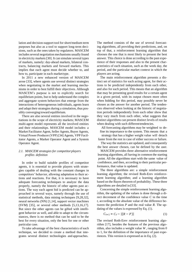
teristics and past actions. This algorithm’s organization

is presented in Fig. 1.

To get warrantable data, agents using this method

perform an analysis of the historical data. With the

gathered information, agents can build a profile of

other agents including information about their ex-

pected proposed prices, limit prices, and capacities.

With these profiles, and based on the agent own objec-

tives, several scenarios, and the possible advantageous

bids for each one, are defined.

Seller and Buyer agents interact with each other, in

MASCEM environment, taking into account that their

results are influenced by competitor’s decisions. Game

theory is well suited for analyzing these kinds of situ-

ations [6,23].

3.1. Scenario definition

MASCEM is implemented as a Decision Support

tool, so the user should have the flexibility to decide

Fig. 1. Scenario analysis algorithm. (Colours are visible in the online

version of the article; http://dx.doi.org/10.3233/ICA-130438)

how many and which scenarios should be analyzed. To

do so, the user must define the scenarios to be sim-

ulated by specifying the price that competitor agents

will propose Eq. (4):

where λ and ϕ are scaling factors that can be different

for each agent and for each scenario.

The Probable_Price is a predicted value concerning

the expected bidding price of each competitor player.

This prediction is reached by using the players’ pro-

files definition mechanism, presented in section 2. This

prediction allows the proposed method to use adequate

and realistic values when considering other players’

actions.

The Limit_Price corresponds to maximum price that

can be bided by a seller agent, or the minimum price

that can be bided by a buyer agent.

Equation (4) is used to provide the definition of al-

ternative scenarios, concerning agents may define bids

between their limit and probable prices.

Let us suppose that the user selects λ = 0 and ϕ = 1

for every Seller and λ = 1 and ϕ = 0 for every Buyer;

this means an analysis of a pessimistic scenario. If the

user selects λ = 1 and ϕ = 0 for every agent, then

the most probable scenario will be analyzed. Using this

formula the user can define for each agent the proposed

prices for every scenario that it desires to consider.

o

scenarios areThe

Each scenario considers a fixed number of players,

each with constant amounts of power. Only the bidding

prices for each player vary from scenario to scenario.

3.2. Bid definition

An agent should analyze the income that results

from bidding its limit, desired, and competitive prices –

those that are just slightly lower (or higher, in the buy-

ers’ case) than its competitors’ prices.

A play is defined as a pair of bid – scenario, so,

the total number of plays to analyze for each player is

Eq. (5):

and the maximum value it can achieve is Eq. (6):

considering that agents only bid their limit or expected

prices. However, an agent may bid prices between its

limit and expected prices, or even above that limit

price. If we consider each agent may bid numprices

prices, the number of scenarios becomes equal to npn,

and the number of plays to analyze is Eq. (7).

The user is also allowed to choose the number of bids

that will be considered as possibilities for the final bid.

In this case, the value of the bids is calculated depend-

ing on an interval of values that can also be defined by

the user. That interval is always centered on a trusted

value, the value of the market price of the same pe-

riod of the previous day. In this way the considered

possible bids are always around that reference value,

and their range of variance depends on the bigger or

smaller value of the user defined interval.

So, being nb the number of bids defined by the user,

int the value defining the interval to be considered, and

mp the market price from the same period of the previ-

ous day, the possible bids b1...nb are defined as Eqs (8)

and (9):

strategy two-player game, assuming each player seeks

to minimize the maximum possible loss or maximize

the minimum possible gain.

After each negotiation period, an agent may in-

crease, decrease or maintain its bid, increasing the

number of scenarios to analyze. So, after k periods,

considering only three possible bid updates, the num-

ber of plays to analyze becomes Eq. (10):

3.3. Game theory for scenario analysis

A seller, like an offensive player, will try to maxi-

mize the minimum possible gain by using the MaxiMin

decision method. A buyer, like a defensive player, will

select the strategy with the smallest maximum payoff

by using the MiniMax decision method.

Buyers’ matrix analysis leads to the selection of only

those situations in which all the consumption needs are

fulfilled. This avoids situations in which agents have

reduced expenses but cannot satisfy their consumption

needs completely.

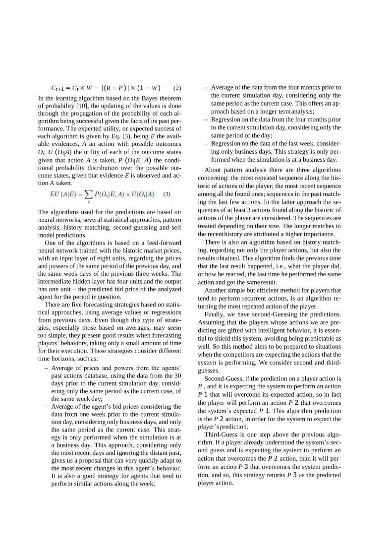
The state space to be searched is related to the possi-

ble plays of other agents, regarding possible bids from

one agent. Figure 2 illustrates this procedure.

Fig. 2. Game theory for scenario-space search. (Colours are vis-

ible in the online version of the article; http://dx.doi.org/10.3233/

ICA-130438)

Each bid of a specific agent (e.g. Agi) is analyzed

by considering several possible scenari s, in order to

After defining all the scenarios and bids, market sim-

ulation is applied to build a matrix with the expected

results for each play.

The matrix analysis with the simulated plays’ results

is inspired on the game theory concepts for a pure-

evaluated by considering the prices other agents may

propose, regarding the previous proposed prices. It is

also considered that each agent may change its price: increasing a lot (↑↑), increasing a little (↑), maintaining

(-), decreasing a little (↓), or decreasing a lot (↓↓) its

support the decision of this agent.

support the decision of this agent.

bid price (A little means from 0 to 10% and a lot from

10% to 30%). Here the concepts of little and lot will

consider the historic data of agents’ bids and will be

converted to variations in cents. It is important to ob-

serve that it is impossible to consider all kind of varia-

tions, due to the complexity of the problem, as we have

seen before. The required time for solving the problem

with a large set of combinations would be impractical

since a complete market simulation is required for each

scenario.

Each leaf node of the tree in Fig. 2 corresponds to

a possible scenario. The idea is to evaluate each one

of these scenarios and apply a MiniMax or MaxiMin

based algorithm to select the safest bid to be offered by

agent Agi.

Notice that our use of game theory is intended for

supporting one specific agent and not for achieving the

equilibrium in the market. The idea of the methodology

proposed in this paper is to provide a specific agent

with decision support.

For each simulated scenario (leaf of Fig. 2) we will

calculate the price Pmarket for each MW.h (Megawatt

hour), defined as the result of the simulated market.

For the support of seller agents the evaluation of the

scenario (in profits, F ) is made by the product of the

energy sold by the supported agent Agi, Energy_Soldi,

by the profit, obtained from the difference between

Pmarket and the cost associated to each MW.h sold by

Agi, Costi, according to Eq. (11):

Notice that the part of this formula that demands the

higher processing cost is the calculation of the value

Pmarket, since it implies to run the simulation of the

scenario in order to determine the market clearing

price.

Additionally, there are two methods for solving

problems of equality in the evaluation of scenarios. In

case of a seller, the MaxiMin algorithm chooses the bid

that offers the maximum gain, from the worst possible

scenario. In case of more than one scenario being eval-

uated with equal value as worst scenario, the options

for choosing among them are:

– a greedy approach, choosing the scenario, among

the equally worst ones, that presents the bid that

allows the higher payoff from all the possible

bids;

– an average of the results of all possible bids for

these scenarios, choosing the one that gets the

worst average as the worst possible scenario.

The user is able to choose among these two meth-

ods for solving the problems of equality. He can also

choose a third option that is a mechanism that chooses

automatically among these two options, accordingly to

the success that each of them is presenting. This mech-

anism uses a reinforcement learning algorithm, with

initial equal values of confidence for the two options.

As the time evolves, the values of success of each op-

tion are updated, and the one that presents the best con-

fidence in each run, is the one chosen.

The updating of these confidence values is per-

formed by running the two options and saving the an-

swer proposed by each one. Later, after the bid is cho-

sen as the agent’s action for the actual market, this

method analyzes the market values and checks which

of the outputs proposed by each method would have

led to the best results.

This procedure is similar to the one used for updat-

ing the values of the players’ profile definition method-

ology, by comparing the values proposed by each of the

algorithms used for forecasting with the actual actions

the each player performed in the market.

The scenario analysis algorithm is implemented in

JAVA,1 for a smoother integration with MASCEM sim-

ulator. However, for efficiency issues, the majority of

data analysis methods, namely the pattern analysis and

history matching algorithms for players’ profiles def-

inition, are implemented in LPA Prolog.2 The neural

network was developed in MatLab.3

4. Experimental findings

This section presents a case study with two main ob-

jectives: (i) understand how to use the proposed ap-

proach, by comparing the performance of different pa-

rameterizations; (ii) compare the results that can be

achieved with the proposed approach and with other

reference decision support strategies.

The results are evaluated by comparing the incomes

that are achieved in an electricity market simulation,

using the different approaches and parameterizations.

4.1. Case study characterization

This case study concerns three simulations under-

taken using MASCEM, referring to the same 16 con-

1http://www.java.com/. 2http://www.lpa.co.uk/. 3http://www.mathworks.com/products/matlab.

secutive days, starting from Friday, 15th October,

2010. The data used in this case study has been based

on real data extracted from the Iberian market – Iberial

Electricity Market – MIBEL [24].

These simulations involve 7 buyers and 5 sellers (3

regular sellers and 2 VPPs). This group of agents was

created with the intention of representing the Iberian

reality, reduced to a smaller group, containing the es-

sential aspects of different parts of the market, al-

lowing a better individual analysis and study of the

interactions and potentiality of each of those actors.

This group of agents results from the studies presented

in [33].

4.1.1. Simulated agents strategic behavior

For these simulations we will consider different bid-

dings for each agent. Seller 2, which will be our test

reference, will use the proposed method with different

parameters in each of the three simulations. This al-

lows comparing the performance of this method when

using distinct parameterizations and taking conclu-

sions on its suitability and the influence of the differ-

ent parameters presented in Section 3. This section ad-

ditionally presents the comparison between the results

obtained by each of the three considered parameteriza-

tions and the results obtained by using two other strate-

gies which are well established and with verified per-

formance and results, in order to determine in what de-

gree the proposed game theory based strategy is best

or worst suited for providing decision support to mar-

ket players. These strategies are: (i) the AMES strat-

egy [20]; (ii) the SA-QL strategy [32].

The AMES strategy is used by the AMES electricity

markets simulator [20] to provide support to the mod-

elled players when bidding in the market. This strat-

egy is based on a study of the efficiency and reliabil-

ity of the Wholesale Power Market Platform (WPMP),

a market design proposed by the U.S. Federal Energy

Regulatory Commission for common adoption by all

U.S. wholesale power markets [11,12]. The AMES

strategy was adapted by the authors of this paper in a

previous work [25], to suit it to the purposes of asym-

metrical and symmetrical pool markets, such as the

Iberian Electricity market – MIBEL [24]. This strategy

uses a reinforcement learning algorithm – the Roth-

Erev algorithm [17] to choose from a set of the pos-

sible actions (or Action Domain) which is based on

the companies’ production costs analysis. Addition-

ally, the Simulated Annealing heuristic [4] is imple-

mented to accelerate the convergence process.

The SA-QL strategy [32] is similar to the AMES

strategy in its fundamentals: the use of a reinforce-

ment learning algorithm to choose the best from a set

of possible actions. The differences concern two main

aspects: the used reinforcement learning algorithm is

the Q-Learning [18] algorithm; and the set of differ-

ent possible bids to be used by the market negotiat-

ing agent is determined by a focus on the most prob-

able points of success (in the area surrounding the ex-

pected market price). This strategy also uses the Sim-

ulated Annealing heuristic to accelerate the process of

convergence.

The other simulated players’ bids are defined as fol-

lows:

– Buyer 1 – This buyer buys power independently

of the market price. The offer price is 18.30

c /kWh (this value is much higher than average

market price).

– Buyer 2 – This buyer bid price varies between two

fixed prices, depending on the periods when it re-

ally needs to buy, and the ones in which the need

is lower. The two variations are 10.00 and 8.00

c /kWh.

– Buyer 3 – This buyer bid price is fixed at 4.90

c /kWh.

– Buyer 4 – This buyer bid considers the average

prices of the last 4 Wednesdays.

– Buyer 5 – This buyer bid considers the average

prices of the last 4 months.

– Buyer 6 – This buyer bid considers the average

prices of the last week (considering only business

days).

– Buyer 7 – This buyer only buys power if market

prices are lower than average market price.

– Seller 1 – This seller needs to sell all the power

that he produces. The offer price is 0.00 c /kWh.

– Seller 3 – This seller bid considers the average

prices of the last 4 months with an increment of

0.5 c /kWh.

– VPP 1 – Includes 4 wind farms and offers a

fixed value along the day. The offer price is 3.50

c /kWh.

– VPP 2 – Includes 1 photovoltaic, 1 co-generation

and 1 mini-hydro plants; the offer price is based

on the costs of co-generation and the total fore-

casted production.

4.1.2. Parameterization

The common parameters in all the simulations using

the game theory strategy are: the selection of the auto-

matic mechanism for solving the problems of equality

among scenarios; for all seller agents the limit price is

fixed as 0 c /kWh, for it does not make sense to bid

Fig. 3. Incomes obtained by Seller 2 in the first period of the

considered 16 days, using: A) the first parameterization, B) the

second parameterization, C) the third parameterization. (Colours

are visible in the online version of the article; http://dx.doi.org/

10.3233/ICA-130438)

negative values; for all buyer agents the limit price is

20 c /kWh, a high value for allowing the players to

consider a good margin of prices. Also, the selected

reinforcement learning algorithm for the players’ pro-

files definition has been the revised Roth-Erev, with

equal value of the algorithms weight. The past expe-

rience weight W value is set to 0.4, a small value to

grant higher influence to the most recent results, so that

it can quickly learn and catch new tendencies in play-

ers’ actions. For each scenario the scaling factors for

competitors’ probable price λ and limit price ϕ, will be

equal for every competitor agent, in order to give the

same importance to the price forecast of each agent.

These scaling factors will only vary from scenario to

scenario, but always maintaining the equality among

agents.

The variations introduced in each simulation are as

follows.

In the first simulation Seller 2 will use the scenario analysis method with a small number of considered

scenarios and possible bids. This test will allow us to perceive if a restrict group of scenarios, and conse-

quent advantage in processing speed, will be reflected

on a big difference in the results quality. For this sim- ulation the number of considered scenarios is 3, the

number of considered bids is 5, and the interval for the possible bids definition is 8. Considering the 3 scenar-

ios, the first will attribute to all agents λ = 1 and ϕ = 0; the second λ = 0,95 and ϕ = 0,05; and the third

λ = 0,9 and ϕ = 0,1. These values give higher impor- tance to the most probable prices, in order to consider

the most realistic scenarios.

In the second simulation Seller 2 will use the sce- nario analysis method with an intermediate number of considered scenarios and possible bids. The number of considered scenarios is 5, the number of considered bids is 7, and the interval for the possible bids defini- tion is 8. Considering the 5 scenarios, the first will at-

tribute to all agents λ = 1 and ϕ = 0; the second λ = 0,95 and ϕ = 0,05; the third λ = 0,9 and ϕ = 0,1; the

fourth λ = 0,8 and ϕ = 0,2; and the fifth λ = 0,7 and

ϕ = 0,3.

Finally, in the third simulation Seller 2 will use the method with a higher number of considered scenarios and possible bids, in order to obtain a more detailed analysis. The number of considered scenarios is 7, the number of considered bids is 10, and the interval for the possible bids definition is 10, granting also a bigger interval for considered bids. Considering the 7 scenar-

ios, the first will attribute to all agents λ = 1 and ϕ = 0; the second λ = 0,95 and ϕ = 0,05; the third λ = 0,9 and ϕ = 0,1; the fourth λ = 0,8 and ϕ = 0,2; the

fifth λ = 0,7 and ϕ = 0,3; the sixth λ = 0,5 and ϕ = 0,5; and the seventh λ = 0,2 and ϕ = 0,8.

After the simulations, the incomes obtained by

Seller 2 using the proposed method with each of the

three combinations of parameters can be compared.

This agent’s power production to be negotiated in the

market will remain constant at 50 MW for each pe-

riod throughout the simulations. Regarding the costs of

all players, they are defined as null, for facilitating the

comparison of the results.

4.2. Results

Since the reinforcement learning algorithm for the

players’ profiles definition treats each period of the day

C

B

A

A

B

comes in the first period of each considered day, along

the 16 days, using each of the three considered combi-

nations of parameters.

Figure 4 Presents the results of Seller 2 in the twelfth

period of each considered day.

Figure 5 presents the comparison between the three

parameterizations of the game theory strategy and the

other two strategies’ performance: The AMES strat-

egy, and the SA-QL.

4.3. Discussion of the results

C

Fig. 4. Incomes obtained by Seller 2 in the twelfth period of the

considered 16 days, using: A) the first parameterization, B) the

second parameterization, C) the third parameterization. (Colours

are visible in the online version of the article; http://dx.doi.org/

10.3233/ICA-130438)

Fig. 5. Total incomes obtained by Seller 2 for the considered 16 days.

as a distinct case, the analysis of the development of

the performance must be done for each period individ-

ually. Figure 3 presents the evolution of Seller 2 in-

Comparing the graphs presented in Fig. 3, it can be

concluded that the first simulation was clearly the most

disadvantageous for Seller 2 for this period. The sec-

ond and third simulations present very similar results

in what concerns the incomes obtained by this agent in

the first period.

The results of the twelfth period (Fig. 4) show the

first parameterization worst results when compared

with the other two. However, in this case, the third pa-

rameterization clearly obtained better results than the

second one. The global results for all periods of the

considered 16 days, presented in Fig. 5, support this

tendency.

From Fig. 5 it is visible that the first parameteriza-

tion presents a large difference from the other two, and

a smaller difference between the results achieved by

the second and third parameterizations can be clearly

seen. The comparison of the different parameteriza-

tions’ performances allows taking an important con-

clusion: when it is required for the simulations to im-

prove the processing times, a criterious reduction of the

search space may not represent a significant decrease

of the method’s effectiveness. As proven by simulation

2, which even though considering fewer scenarios and

possible bids than the parameterization of simulation 3,

its results were still acceptable for situations for which

the method’s processing time is crucial.

Regarding the comparison between the use of the

game theory strategy and the other two comparing

strategies, it is visible that the first parameterization

of the proposed strategy achieves lower results than

the two reference strategies. This was expected and it

is easily justified by the low number of scenarios and

possible bids that this parameterization concerned. The

second parameterization achieves very similar results

to the ones obtained by the two reference strategies.

This means that, even using an intermediate number of

scenarios and bids, the proposed game theory strategy

is capable of achieving levels of performance that are

similar to the results of reference and well established

strategies. In what concerns to the third parameteriza-

tion, it is capable of achieving best results than any of

the other strategies, for the considered days. This is a

motivating result, suggesting that the proposed method

is able to provide better results to a market negotiat-

ing player’s actions, when the parameters are suitably

defined.

5. Conclusions and future work

This paper proposed a computational model for bid

definition in electricity markets. The proposed model

comprises the definition of markets scenarios, concern-

ing different perspectives and the electricity markets

evolution; other players profiles definitions, based on

the analysis of the gathered information through pre-

diction algorithms; the establishment of a set of pos-

sible actions taking into account each current context

and the adaptation of the game theory concept to the

electricity market negotiation environment, intended

for supporting one specific agent and not for achieving

the equilibrium in the market. The proposed method

was integrated in MASCEM, an electricity market sim-

ulator developed by the authors’ research centre.

The model proves to be adequate for providing deci-

sion support to electricity markets players, allowing an

analysis of different scenarios, taking into account the

predictions of competitor players’ actions.

The results presented in the experimental findings

section show that it can achieve good results when

using suitable parameterizations, as in simulation 3.

These good results are also shown not to be directly

proportional to the scenarios search space, which is a

relevant aspect when dealing with timely exigent sim- ulations. This conclusion facilitates the adaptability of

analysis in the neighborhood of the scenario selected

by the algorithm. To achieve this, an evolutionary ap-

proach will be included and combined with the game

theory.

Acknowledgments

This work is supported by FEDER Funds through

COMPETE program and by National Funds through

FCT under the projects FCOMP-01-0124-FEDER:

PEst-OE/EEI/UI0760/2011, PTDC/EEA-EEL/099832

/2008, PTDC/SEN-ENR/099844/2008, PTDC/SEN-E

NR/122174/2010 and PTDC/EEA-EEL/122988/2010.

References

[1] M. Ahmadlou and H. Adeli, Enhanced Probabilistic Neural

Network with Local Decision Circles: A Robust Classifier,

Integrated Computer-Aided Engineering 17(3) (2010), 197–

210.

[2] R. Badaway, B. Hirch and S. Albayrak, Agent-Based Co-

ordination Techniques for Matching Supply and Demand in

Energy Networks, Integrated Computer-Aided Engineering

17(4) (2010), 373–382.

[3] R. Badawy, A. Yassine, A. Heßler, B. Hirsch and S. Albayrak,

A Novel Multi-Agent System Utilizing Quantum-Inspired

Evolution for Demand Side Management in the Future Smart

Grid, Integrated Computer-Aided Engineering 20(2) (2013),

127–141.

[4] S. Bandyopadhyay, Multiobjective Simulated Annealing for

Fuzzy Clustering With Stability and Validity, IEEE Transac-

tions on Systems, Man, and Cybernetics, Part C: Applications

and Reviews 41(5) (2011), 682–691.

[5] P. Baraldi, R. Canesi, E. Zio, R. Seraoui and R. Chevalier, Ge-

netic algorithm-based wrapper approach for grouping condi-

tion monitoring signals of nuclear power plant components,

Integrated Computer-Aided Engineering 18(3) (2011), 221–

234.

[6] S. Ceppi and N. Gatti, An algorithmic game theory study of

wholesale electricity markets based on central auction, Inte-

the decision making process regarding the method’s ef-

ficiency and effectiveness.

Additionally, when comparing the results of the pro- posed game theory strategy with the performance of

[7]

grated Computer-Aided Engineering 17(1) (2010), 273–290.

B. Chen and W. Liu, Mobile Agent Computing Paradigm for

Building a Flexible Structural Health Monitoring Sensor Net-

work, Computer-Aided Civil and Infrastructure Engineering

25(7) (2010), 504–516.

two other well documented and reference strategies, it

was found that this strategy is capable of achieving best

results when the parameters are defined correctly. In

fact, even when opting by a faster but less broad ap-

proach (parameterization with less considered scenar-

ios and a smaller action domain), the game theory strat-

egy was still able to achieve results in the same range

as the reference strategies.

Considering the improvement of this method, fur-

ther work will be done in what concerns a detailed

[8] L. Cristaldi, F. Ponci, M. Faifer and M. Riva, Multi-agent Sys-

tems: an Example of Power System Dynamic Reconfigura-

tion, Integrated Computer-Aided Engineering 17(4) (2010),

359–372.

[9] A. Dahabiah, J. Pontes and B. Solaiman, Fusion of possibilis-

tic sources of evidences for pattern recognition, Integrated

Computer-Aided Engineering 17(2) (2010), 117–130.

[10] A. Dore and C. Regazzoni, Interaction Analysis with a

Bayesian Trajectory Model, IEEE Intelligent Systems 25(3)

(2010), 32–40.

[11] Federal Energy Regulatory Commission, Notice of White

Paper, U.S. Federal Energy Regulatory Commission 4(28)

(2003).

[12] Federal Energy Regulatory Commission, Report to Congress

on competition in the wholesale and retail markets for elec-

tric energy, U.S. Federal Energy Regulatory Commission.

Available: http://www.ferc.gov/legal/maj-ord-reg/fed-sta/ene-

pol-act/epact-final-rpt.pdf.

[13] A.J. Fougères and E. Ostrosi, Fuzzy agent-based approach

for consensual design synthesis in product configuration, Inte-

grated Computer-Aided Engineering 20(3) (2013), 259–274.

[14] S. Freitag, W. Graf and M. Kaliske, Recurrent neural networks

for fuzzy data, Integrated Computer-Aided Engineering 18(1)

(2011), 265–280.

[15] J.O. Gutierrez-Garcia and K.M. Sim, Agent-based Cloud

Workflow Execution, Integrated Computer-Aided Engineer-

ing 19(1) (2012), 39–56.

[16] B. Heilmann, N.E. El Faouzi, O. de Mouzon, N. Hainitz,

H. Koller, D. Bauder and C. Antoniou, Predicting Motorway

Traffic Performance by Data Fusion of Local Sensor Data and

Electronic Toll Collection Data, Computer-Aided Civil and

Infrastructure Engineering 26(6) (2011), 451–463.

[17] Z. Jing, H.W. Ngan, Y.P. Wang, Y. Zhang and J.H. Wang,

Study on the convergence property of re learning model in

electricity market simulation, Advances in Power System

Control, Operation and Man-agement, 2009.

[18] C. Juang and C. Lu, Ant Colony Optimization Incor-porated

With Fuzzy Q-Learning for Reinforcement Fuzzy Control,

IEEE Transactions on Systems, Man and Cybernetics, Part A:

Systems and Humans 39(3) (2009), 597–608.

[19] V. Koritarov, Real-World Market Representation with Agents:

Modeling the Electricity Market as a Complex Adaptive Sys-

tem with an Agent-Based Approach, IEEE Power and Energy

magazine (2004), 39–46.

[20] H. Li and L. Tesfatsion, Development of Open Source Soft-

ware for Power Market Research: The AMES Test Bed, Jour-

nal of Energy Markets 2(2) (2009), 111–128.

[21] Y. Lim, H.M. Kim, S. Kang and T. Kim, Vehicle-to-Grid

Communication System for Electric Vehicle Charging, Inte-

grated Computer-Aided Engineering 19(1) (2012), 57–65.

[22] A. Nejat and I. Damnjanovic, Agent-based Modeling of Be-

havioral Housing Recovery Following Disasters, Computer-

Aided Civil and Infrastructure Engineering 27(10) (2012),

748–763.

[23] J. Neumann, The essence of game theory, IEEE Potentials

22(2) (2003).

[24] Operador del Mercado Ibérico de Energia, Polo Español –

homepage, http://www.omie.es, accessed on December 2011.

[25] T. Pinto, Z. Vale, F. Rodrigues, I. Praca and H. Morais, Cost

Dependent Strategy for Electricity Markets Bidding Based on

Adaptive Reinforcement Learning, International Conference

on Intelligent System Application on Power Systems – ISAP,

2011.

[26] I. Praça, C. Ramos, Z. Vale and M. Cordeiro, MASCEM: A

Multi-Agent System that Simulates Competitive Electricity

Markets, IEEE Intelligent Systems – Special Issue on Agents

and Markets 18(6) (2003), 54–60.

[27] M. Prymek and A. Horak, Multi-agent Approach to Power

Distribution Network Modelling, Integrated Computer-Aided

Engineering 17(4) (2010), 291–303.

[28] U. Reuter, A Fuzzy Approach for Modelling Non-stochastic

Heterogeneous Data in Engineering Based on Cluster Anal-

ysis, Integrated Computer-Aided En-gineering 18(3) (2011),

281–289.

[29] E.J. Rodrıguez-Seda, D.M. Stipanovic and M.W. Sponga,

Teleoperation of Multi-Agent Systems with Nonuniform Con-

trol Input Delays, Integrated Computer-Aided Engineering

19(2) (2012), 125–136.

[30] G. Santos, T. Pinto, H. Morais, I. Praca and Z. Vale, Complex

Market integration in MASCEM electricity market simulator,

International Conference on the European Energy Market 11 –

EEM, 2011.

[31] M. Shahidehpour, H. Yamin and Z. Li, Market Operations in

Electric Power Systems: Forecasting, Scheduling, and Risk

Management, Wiley-IEEE Press, 2002, pp. 233–274.

[32] A. Tellidou and A. Bakirtzis, Agent-Based Analysis of

Monopoly Power in Electricity Markets’, International Con-

ference on Intelligent Systems Applications to Power Sys-

tems, 2007.

[33] Z. Vale, T. Pinto, I. Praça and H. Morais, MASCEM – Elec-

tricity markets simulation with strategic players, IEEE Intel-

ligent Systems – Special Issue on AI in Power Systems and

Energy Markets 26(2) (2011), 54–60.

[34] Z. Vale, T. Pinto, H. Morais, I. Praça and P. Faria, VPP’s

Multi-Level Negotiation in Smart Grids and Competitive

Electricity Markets, IEEE PES General Meeting – PES-GM,

2011.

[35] E. Wandekokem, E. Mendel, F. Fabris, M. Valentim, R.

Batista, F. Varejão and T. Rauber, Diagnosing multiple faults

in oil rig motor pumps using support vector machine classifier

ensembles, Integrated Computer-Aided Engineering 18(1)

(2011), 61–74.