strategic jet engine system design in light of …eprints.soton.ac.uk/196689/1/atio_paper.pdf ·...

American Institute of Aeronautics and Astronautics

1

Strategic Jet Engine System Design in Light of Uncertain

Fuel and Carbon Prices

Stephan Langmaak1, James Scanlan2, and András Sóbester3 University of Southampton, Southampton, SO17 1BJ, United Kingdom

Stephen Wiseall4 Rolls-Royce plc, Derby, DE24 8BJ, United Kingdom

This paper presents a project that is investigating which cruise speed the next generation

of short-haul aircraft with 150 seats should fly at and which combination of advanced engine

technologies should be employed in order to make the profit generated by the aircraft robust

to uncertain fuel and carbon prices in Europe in 2030. To answer this question, an

optimization loop is being set up in MATLAB consisting of five modules, including an

aircraft design, a travel demand, a modal shift, a flight profile, and an engine design

element. The first three modules were tested in a preliminary study that analyzed the effect

of high and low fuel and carbon prices on the optimum aircraft design and its ideal cruise

speed. The results indicate that if oil and CO2 prices were to rise significantly, a slower

turboprop aircraft would be more profitable in terms of Surplus Value in comparison to a

conventional turbofan design. If prices were to reduce, however, a faster turbofan aircraft

would offer a superior business case. The study also showed that making realistic Surplus

Value predictions is more difficult than forecasting costs.

Nomenclature

CD = drag coefficient D = drag, N S = wing reference area, m2

s = distance, m

V = velocity, m/s W = work done, J ρ = density, kg/m3

I. Introduction

A. Project Incentive t takes around 5 years to develop a jet engine, which then usually remains in production for more than two decades1,2. Similar to the rest of the aerospace industry, gas turbine makers therefore have to make multi-billion investments into these large and long-term projects and it normally takes at least 15 years until the costs are

recuperated1. Consequently, the strategic design team must make a sound prediction 30 years into the future and optimize the product in such a way that it remains competitive throughout that period.

When optimizing a design, its performance should not simply be maximized by taking the product to its limits where a slight perturbation could lead to a significant loss in performance. Instead, the design should be made more

1 EngD Research Engineer, Computational Engineering and Design, Faculty of Engineering and the Environment, Student Member. 2 Professor of Design, Computational Engineering and Design, Faculty of Engineering and the Environment, AIAA Member. 3 Lecturer, Computational Engineering and Design, Faculty of Engineering and the Environment, AIAA Member. 4 Team Leader, Product Cost Systems, PO Box 31.

I


2

robust by placing it on a performance plateau within the design space where the variability has a minimum effect on the performance3.

In 2008, Flightglobal* reported that: Rolls-Royce [an aircraft engine manufacturer] is talking up the possibility of a new generation of turboprop-powered aircraft replacing a substantial proportion of today’s narrowbody jets. The manufacturer believes high oil prices are likely to drive airframers to sacrifice cruise speed for economics. “The TP400 engine [for the Airbus A400M military transport] is a very efficient propulsion system,” R-R Director Engineering and Technology, Colin Smith, says. “There is a very sound argument to be made for the majority of the 150-seat market, which flies mostly for less than 1.5h [being turboprop-powered]...”

Thus, this project will use Robust Design theory to find the ideal cruise speed and the optimum combination of various advanced jet engine technologies to maximize the profitability of the next generation of short-range 150-seater aircraft in light of uncertain oil and carbon prices in Europe in 2030.

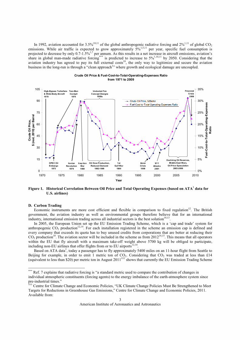
B. Fuel Price Variability Between 1971 and 2009, the 12-month average oil price fluctuated between $15 and over $90 per barrel in 2010

prices, which in turn caused the fuel cost fraction to vary between 10% and over 30% of the total operating expenses of U.S. airlines†, as Fig. 1 shows.

Although less than half of the planet’s crude oil reserves have been used up, the remaining oil will be more difficult and expensive to extract, which will slow production, increase oil prices and have controversial environmental and social impacts‡,§. Various independent sources forecast that maximum oil extraction will occur between 2009 and 2031 and there is a significant risk that it will happen before 2020**,††,‡‡,1. Although the decline will not be sudden, the equivalent of a new Saudi Arabia has to be tapped every three years and more than two thirds of the current oil production capacity has to be replaced by 20304. Sir Richard Branson, the founder of the Virgin Group, expects that “the next five years will see us face another crunch: the oil crunch§§.”

In July 2008, jet fuel prices peaked at $4.33 per U.S. gallon, but plummeted to $1.28 by late December that year5. Although historically that is an extreme example, the previous paragraph explained why high and erratic oil prices‡ will become more common in the future. After the current recession, fuel cost is therefore likely to represent the biggest part of the total operating expenses of U.S. airlines again, as between 2006 and 2008. Although “air ticket prices have reached their lowest level and will never be as low again1,” air cargo is even more affected by fuel prices because there are no additional passenger-related costs5.

Due to the lack of data transparency, oil price projection is a matter of debate rather than science**. It is therefore not surprising that various institutions predict significantly different oil prices, even in the short term. Consequently, the forecasts various sources make for 2030 vary between $55 and $305 per barrel in 2008 prices6-9.

C. Aircraft Emissions

According to Ref. 1, global CO2 equivalent emissions have to drop by 50-85% by 2050 relative to the year 2000

to ensure that pre-industrial temperatures are not exceeded by more than 2.0 to 2.4 °C on average. In order to meet this target, “all industry sectors, including aviation, need to contribute their share of emissions reduction1.”

* Daly, K., “Rolls-Royce Promotes Turboprop Solution for New Civil Airliners,” Flightglobal, 2008. Available from: http://www.flightglobal.com/articles/2008/07/01/224987/rolls-royce-promotes-turboprop-solution-for-new-civil.html † Air Transport Association (ATA) Quarterly Cost Index for U.S. Passenger Airlines. Available from: http://www.airlines.org/Economics/DataAnalysis/Pages/QuarterlyCostIndex.aspx ‡ Guardian.co.uk, “Peak Oil Could Hit Soon, Report Says,” The Guardian, 2009. Available from: http://www.guardian.co.uk/environment/2009/oct/08/peak-oil-could-hit-soon § Saven, J., “Peak Oil Predictions,” The Guardian, 2010. Available from: http://www.guardian.co.uk/commentisfree/2010/apr/23/peak-oil-energy-recession ** Porter, A., “’Peak Oil’ Enters Mainstream Debate,” BBC News, 2005. Available from: http://news.bbc.co.uk/1/hi/4077802.stm †† Schultz, S., “Military Study Warns of a Potentially Drastic Oil Crisis,” Spiegel Online International, 2010. Available from: http://www.spiegel.de/international/germany/0,1518,715138,00.html ‡‡ Connor, S., “Warning: Oil Supplies Are Running Out Fast,” The Independent, 2009. Available from: http://www.independent.co.uk/news/science/warning-oil-supplies-are-running-out-fast-1766585.html §§ Guardian.co.uk, “Energy Minister Will Hold Summit to Calm Rising Fears Over Peak Oil,” The Guardian, 2010. Available from: http://www.guardian.co.uk/business/2010/mar/21/peak-oil-summit


3

In 1992, aviation accounted for 3.5%10,11 of the global anthropogenic radiative forcing and 2%1,11 of global CO2 emissions. While air traffic is expected to grow approximately 5%1,5,11 per year, specific fuel consumption is projected to decrease by only 0.7-1.5%1,7 per annum. As this results in a net increase in aircraft emissions, aviation’s share in global man-made radiative forcing*** is predicted to increase to 5%1,10,11 by 2050. Considering that the aviation industry has agreed to pay its full external costs10, the only way to legitimize and secure the aviation business in the long-run is through a “clean approach1” where growth and ecological damage are uncoupled.

D. Carbon Trading Economic instruments are more cost efficient and flexible in comparison to fixed regulation12. The British

government, the aviation industry as well as environmental groups therefore believe that for an international industry, international emission trading across all industrial sectors is the best solution10,13.

In 2005, the European Union set up the EU Emission Trading Scheme, which is a ‘cap and trade’ system for anthropogenic CO2 production

12,14. For each installation registered in the scheme an emission cap is defined and every company that exceeds its quota has to buy unused credits from corporations that are better at reducing their CO2 production

10. The aviation sector will be included in the scheme as from 201214,15. This means that all operators within the EU that fly aircraft with a maximum take-off weight above 5700 kg will be obliged to participate, including non-EU airlines that offer flights from or to EU airports12,14.

Based on ATA data†, today a passenger has to fly approximately 5400 miles on an 11-hour flight from Seattle to Beijing for example, in order to emit 1 metric ton of CO2. Considering that CO2 was traded at less than £14 (equivalent to less than $20) per metric ton in August 2011††† shows that currently the EU Emission Trading Scheme

*** Ref. 7 explains that radiative forcing is “a standard metric used to compare the contribution of changes in individual atmospheric constituents (forcing agents) to the energy imbalance of the earth-atmosphere system since pre-industrial times.” ††† Centre for Climate Change and Economic Policies, “UK Climate Change Policies Must Be Strengthened to Meet Targets for Reductions in Greenhouse Gas Emissions,” Centre for Climate Change and Economic Policies, 2011. Available from:

Crude Oil Price & Fuel-Cost-to-Total-Operating-Expenses Ratio

from 1971 to 2009

0

15

30

45

60

75

90

105

1970 1975 1980 1985 1990 1995 2000 2005 2010

Year

Crude Oil Price,

$ (real, 2010) per Barrel

0%

5%

10%

15%

20%

25%

30%

35%

Fuel-Cost-to-Total-Operating-Expenses

Ratio

OPEC Oil

Embargo

1973

Iranian

Revolution

1979

1st

Gulf War

1990

Financial

Crisis

2008

Unducted Fan

Concept Designs

1980s

Oil Over-Production,

Reduced Demand

1982-1988

Declining Oil Reserves,

Middle East Wars,

Oil Price Speculation

2003-2008

High-Bypass Turbofans

& Wide-Body Aircraft

1970

Two-Man

Cockpit

1974

Asian

Crisis

1998

9/11

Attacks

2001

Iraq-Iran

War

1980

Figure 1. Historical Correlation Between Oil Price and Total Operating Expenses (based on ATA

† data for

U.S. airlines)


4

would have a relatively small impact on ticket prices in comparison to the predicted increases in fuel cost15. In order to achieve significant emission reductions and encourage airlines to operate the latest generation of aircraft, 1 metric ton of CO2 would have to cost between €100 and €300

15, i.e. between $140 and $420 using the average exchange rate for August 2011. The independent UK Committee on Climate Change7 predicts that 1 metric ton of CO2 will cost between £35 and £105 in 2030 (approximately $60 to $180 using the exchange rate for August 2011).

E. Uncertain Future The Advisory Council for Aeronautics Research in Europe (ACARE) states: “The future is uncertain, except that

changes will be rapid and marked, especially in the price of resources, and this scenario will become a normal phenomenon1.” Based on the maximum and minimum oil and carbon price estimates for 2030 mentioned previously and a fuel efficiency improvement of 1.0% per annum, the pessimistic total operating expenses prediction for U.S. airlines for 2030 in Fig. 2 is twice as high as the optimistic one. This implies that it is extremely difficult for jet engine manufacturers to design a product that is guaranteed to still be successful several decades later. This challenge could be met with the aid of a jet engine design tool that takes the underlying uncertainty of future oil and carbon prices into account.

http://www.cccep.ac.uk/newsAndMedia/Releases/2011/MR180811_uk-climate-change-policies.aspx

Total Operating Expenses Breakdown for 2008

in ¢ (real, 2010) per Available Seat Mile (ASM)

Other:

6.85 ¢/ASM

44% of total

Ow nership:

0.90 ¢/ASM

6% of total

Labour:

3.08 ¢/ASM

20% of total

Fuel:

4.73 ¢/ASM

30% of total

Total:

15.57 ¢/ASM

Pessimistic Total Operating Expenses Breakdown Prediction for 2030


Other:

6.25 ¢/ASM

24% of total

Ow nership:

0.95 ¢/ASM

4% of total

Labour:

3.28 ¢/ASM

13% of total

Carbon:

2.00 ¢/ASM

8% of total

Fuel:

13.36 ¢/ASM

51% of total

- crude oil price assumption: 305 $/Barrel (real, 2010)

- carbon price assumption: 105 £/tCO2 (real, 2010)

- other operating expenses extrapolated

- technology improvement taken into account

- total cost increase (compared to 2008): 66%

Total:

25.84 ¢/ASM

Optimistic Total Operating Expenses Breakdown Prediction for 2030


Fuel:

2.42 ¢/ASM

18% of total

Carbon:

0.67 ¢/ASM

5% of total

Labour:

3.28 ¢/ASM

24% of total

Ow nership:

0.95 ¢/ASM

7% of total

Other:

6.25 ¢/ASM

46% of total

Total:

13.57 ¢/ASM

- crude oil price assumption: 55 $/Barrel (real, 2010)

- carbon price assumption: 35 £/tCO2 (real, 2010)

- other operating expenses extrapolated

- technology improvement taken into account

- total cost reduction (compared to 2008): 13%

Figure 2. Total Operating Expenses Pie Charts for 2008 and a Pessimistic and Optimistic Prediction for

2030 (based on ATA† data for U.S. airlines and other sources

6,7)


5

II. Advanced Jet Engine Technologies

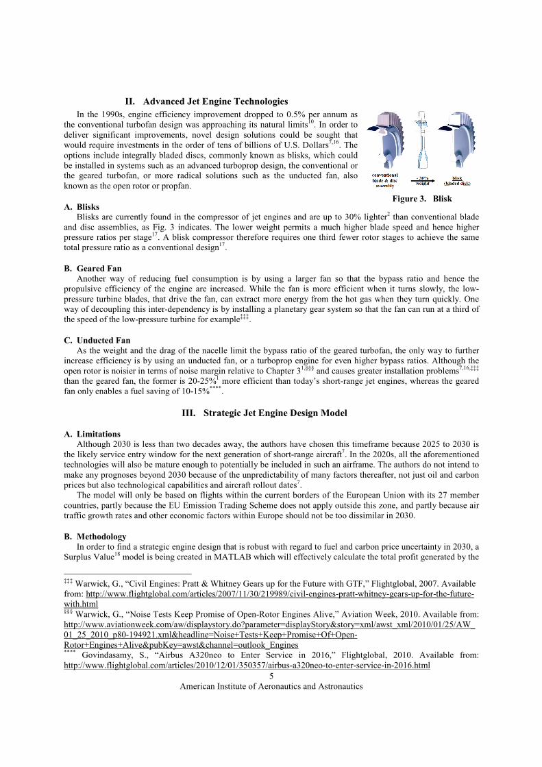
In the 1990s, engine efficiency improvement dropped to 0.5% per annum as the conventional turbofan design was approaching its natural limits10. In order to deliver significant improvements, novel design solutions could be sought that would require investments in the order of tens of billions of U.S. Dollars7,16. The options include integrally bladed discs, commonly known as blisks, which could be installed in systems such as an advanced turboprop design, the conventional or the geared turbofan, or more radical solutions such as the unducted fan, also known as the open rotor or propfan.

A. Blisks Blisks are currently found in the compressor of jet engines and are up to 30% lighter2 than conventional blade

and disc assemblies, as Fig. 3 indicates. The lower weight permits a much higher blade speed and hence higher pressure ratios per stage17. A blisk compressor therefore requires one third fewer rotor stages to achieve the same total pressure ratio as a conventional design17.

B. Geared Fan

Another way of reducing fuel consumption is by using a larger fan so that the bypass ratio and hence the propulsive efficiency of the engine are increased. While the fan is more efficient when it turns slowly, the low-pressure turbine blades, that drive the fan, can extract more energy from the hot gas when they turn quickly. One way of decoupling this inter-dependency is by installing a planetary gear system so that the fan can run at a third of the speed of the low-pressure turbine for example‡‡‡.

C. Unducted Fan As the weight and the drag of the nacelle limit the bypass ratio of the geared turbofan, the only way to further

increase efficiency is by using an unducted fan, or a turboprop engine for even higher bypass ratios. Although the open rotor is noisier in terms of noise margin relative to Chapter 31,§§§ and causes greater installation problems7,16,‡‡‡ than the geared fan, the former is 20-25%1 more efficient than today’s short-range jet engines, whereas the geared fan only enables a fuel saving of 10-15%****.

III. Strategic Jet Engine Design Model

A. Limitations

Although 2030 is less than two decades away, the authors have chosen this timeframe because 2025 to 2030 is the likely service entry window for the next generation of short-range aircraft7. In the 2020s, all the aforementioned technologies will also be mature enough to potentially be included in such an airframe. The authors do not intend to make any prognoses beyond 2030 because of the unpredictability of many factors thereafter, not just oil and carbon prices but also technological capabilities and aircraft rollout dates7.

The model will only be based on flights within the current borders of the European Union with its 27 member countries, partly because the EU Emission Trading Scheme does not apply outside this zone, and partly because air traffic growth rates and other economic factors within Europe should not be too dissimilar in 2030.

B. Methodology

In order to find a strategic engine design that is robust with regard to fuel and carbon price uncertainty in 2030, a Surplus Value18 model is being created in MATLAB which will effectively calculate the total profit generated by the

‡‡‡ Warwick, G., “Civil Engines: Pratt & Whitney Gears up for the Future with GTF,” Flightglobal, 2007. Available from: http://www.flightglobal.com/articles/2007/11/30/219989/civil-engines-pratt-whitney-gears-up-for-the-future-with.html §§§ Warwick, G., “Noise Tests Keep Promise of Open-Rotor Engines Alive,” Aviation Week, 2010. Available from: http://www.aviationweek.com/aw/displaystory.do?parameter=displayStory&story=xml/awst_xml/2010/01/25/AW_01_25_2010_p80-194921.xml&headline=Noise+Tests+Keep+Promise+Of+Open-Rotor+Engines+Alive&pubKey=awst&channel=outlook_Engines **** Govindasamy, S., “Airbus A320neo to Enter Service in 2016,” Flightglobal, 2010. Available from: http://www.flightglobal.com/articles/2010/12/01/350357/airbus-a320neo-to-enter-service-in-2016.html

Figure 3. Blisk


6

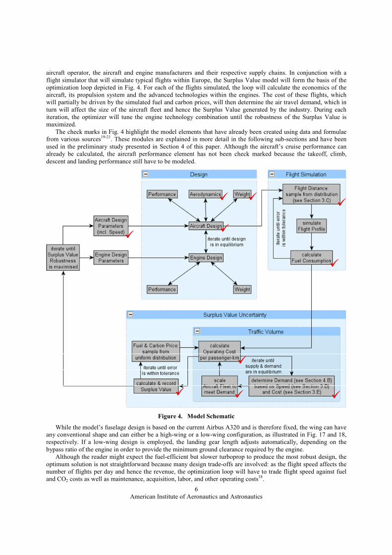
aircraft operator, the aircraft and engine manufacturers and their respective supply chains. In conjunction with a flight simulator that will simulate typical flights within Europe, the Surplus Value model will form the basis of the optimization loop depicted in Fig. 4. For each of the flights simulated, the loop will calculate the economics of the aircraft, its propulsion system and the advanced technologies within the engines. The cost of these flights, which will partially be driven by the simulated fuel and carbon prices, will then determine the air travel demand, which in turn will affect the size of the aircraft fleet and hence the Surplus Value generated by the industry. During each iteration, the optimizer will tune the engine technology combination until the robustness of the Surplus Value is maximized.

The check marks in Fig. 4 highlight the model elements that have already been created using data and formulae from various sources19-21. These modules are explained in more detail in the following sub-sections and have been used in the preliminary study presented in Section 4 of this paper. Although the aircraft’s cruise performance can already be calculated, the aircraft performance element has not been check marked because the takeoff, climb, descent and landing performance still have to be modeled.

While the model’s fuselage design is based on the current Airbus A320 and is therefore fixed, the wing can have

any conventional shape and can either be a high-wing or a low-wing configuration, as illustrated in Fig. 17 and 18, respectively. If a low-wing design is employed, the landing gear length adjusts automatically, depending on the bypass ratio of the engine in order to provide the minimum ground clearance required by the engine.

Although the reader might expect the fuel-efficient but slower turboprop to produce the most robust design, the optimum solution is not straightforward because many design trade-offs are involved: as the flight speed affects the number of flights per day and hence the revenue, the optimization loop will have to trade flight speed against fuel and CO2 costs as well as maintenance, acquisition, labor, and other operating costs

18.

�

��

�

��

�

�

��

��

�

��

�

�

�

Figure 4. Model Schematic


7

C. Air Traffic Model

The flight distances simulated will be sampled from the lognormal distribution shown in Fig. 5. It is based on the direct distances between 30 representative European cities, which are displayed in Fig. 6, and weighting each city pair according to the number of inhabitants. Assuming that that by 2030, flights per capita will be similar throughout Europe, this means that a connection London-Madrid with a combined population of 10.5 million is sampled more often than Luxembourg-Edinburgh with 0.5 million for example.

The maximum flight distance within Europe is 3350 km between Helsinki/Finland and Lisbon/Portugal but the current Airbus A320 is capable of flying almost twice the distance22. Figure 5’s 70th percentile of 1550 km therefore agrees reasonably well with Airbus’ general prediction that “single-aisle aircraft will be overwhelmingly flown on short flights and by 2028, 70% of them will be used on flights of 1850 kilometers or less5.”

D. Modal Shift

Ignoring slow methods of passenger trans-port, including ships, busses, and conventional trains, that barely compete with air travel, the remaining options are: the car, the high-speed train, and the plane itself. Figure 7 shows how the traveling times of these three modes of transport are affected by the direct travel distance.

The graphs for the train and the plane (with an average cruise speed of 812 km/h) are linear regressions of the official travel times obtained from airline and train operator websites that offer transport services between the 40 city pairs in Fig. 6 that have a high-speed rail con-nection. In order to account for actual door-to-door times, 75 minutes†††† were added to the train times and 3 hours‡‡‡‡ to the flight times. The traveling times by car are based on the routes recommended by Google Maps§§§§ which are on average 25% further than the direct distance. The driving times were then calculated by assuming that it takes 7.5 minutes to get to the car, load it, and exit the parking place, and the same time for the reverse process at the final destination. Further assumptions include that the first and the last 12.5 km are done at 50 km/h and the remaining distance at 100 km/h, while having a 15-minute break every 2 hours.

†††† 30 minutes to get to the train, 15 minutes to buy a ticket and board the train, and 30 minutes to travel to the final destination. ‡‡‡‡ 1 hour to get to the airport, 1 hour to check in and board the aircraft, and 1 hour to travel to the final destination. §§§§ Google, “Google Maps,” Google Inc., 2011. Available from: http://maps.google.co.uk

Figure 5. Flight Distance Distribution

Figure 6. Simulated Flight Network

0

2

4

6

8

10

12

14

0 100 200 300 400 500 600 700 800 900

Direct Distance, km

Travelling Tim

e, hours

Plane (812 km/h)

Plane (765 km/h)

Train

Car

Figure 7. Travelling Time Vs. Distance for Different Modes

of Transport


8

Figure 7 indicates that the high-speed train first outpaces the car at distances above 160 km, before the plane first overtakes the car after 237 km and then the train after 273 km. The modal shift illustrated in Fig. 8, which is based on a similar diagram in Ref. 20, lags be-hind these travel time trends, however. The reason the market shares of the train and the plane only start to increase after they outrun the car is because the mobility and flexibility offered by the car gives it a natural advantage in terms of market dominance. Figure 8 would of course look very different for city pairs that do not have a high-speed rail connection. The authors assume, however, that by 2030 many European metropolises will have access to the European high-speed rail network as planned by the European Commission23.

In order to include the effect of the modal shift on the air travel demand in 2030, the authors assumed that the market share of the plane is dependent on the average speed from door to door. For short-haul flights, the average speed is primarily determined by the flight distance and to a lesser extent by the cruise speed, as the graphs for today’s cruise speed of 812 km/h and a potential future cruise speed of 765 km/h in Fig. 9 show. Although Fig. 8 confirms that reducing the cruise speed to 765 km/h has a negligible impact on the market share, the effect becomes more signifi-cant if the cruise speed is reduced below 500 km/h.

E. Demand Elasticity and Air Traffic Growth Scenarios

According to Airbus5, the demand elasti-city of domestic European air travel is -0.96, which means that the demand decreases by ap-proximately 0.96% if prices increase by 1% for example, as Fig. 10 explains.

In their Long-Term Forecast24, the Euro-pean Organisation for the Safety of Air Navi-gation, EUROCONTROL, presents five dif-ferent growth scenarios for the European air traffic between the year 2010 and 2030. Two of these, the best-case scenario ‘A’ and the worst-case scenario ‘E’, which are defined in Table 1, were used in conjunction with Fig. 10’s demand elasticity function to con-figure the authors’ traffic demand module shown in Fig. 4 and Fig. 11.

0%

10%

20%

30%

40%

50%

60%

70%

80%

90%

100%

0 100 200 300 400 500 600 700 800 900

Direct Distance, km

Market Share (in term

s of total trips) Plane (812 km/h)

Plane (765 km/h)

Train

Car

Figure 8. Market Share Vs. Distance for Different Modes of

Transport

0

20

40

60

80

100

120

140

160

180

200

0 100 200 300 400 500 600 700 800 900

Direct Distance, km

Average Speed, km/h

Plane (812 km/h)

Plane (765 km/h)

Train

Car

Figure 9. Average Speed Vs. Distance for Different Modes of

Transport

0%

50%

100%

150%

200%

250%

0% 50% 100% 150% 200% 250%

Relative Price

Relative Demand

Elasticity of -0.96 means:1% increase in price ~ 0.96% decrease in demand

50% reduction in price = 95% increase in demand

100% increase in price = 49% reduction in demand

ln(demand)

ln(price)Elasticity =

Figure 10. Price Elasticity of Demand


9

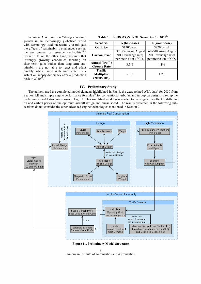
Scenario A is based on “strong economic growth in an increasingly globalised world with technology used successfully to mitigate the effects of sustainability challenges such as the environment or resource availability24.” Scenario E, on the other hand, assumes that “strongly growing economies focusing on short-term gains rather than long-term sus-tainability are not able to react and adapt quickly when faced with unexpected per-sistent oil supply deficiency after a production peak in 202024.”

IV. Preliminary Study

The authors used the completed model elements highlighted in Fig. 4, the extrapolated ATA data† for 2030 from Section 1.E and simple engine performance formulae21 for conventional turbofan and turboprop designs to set up the preliminary model structure shown in Fig. 11. This simplified model was needed to investigate the effect of different oil and carbon prices on the optimum aircraft design and cruise speed. The results presented in the following sub-sections do not consider the other advanced engine technologies mentioned in Section 2.

Figure 11. Preliminary Model Structure

Table 1. EUROCONTROL Scenarios for 203024

Scenario A (best-case) E (worst-case)

Oil Price $130/barrel $220/barrel

Carbon Price

€37 ($52 using August 2011 exchange rate) per metric ton of CO2

€60 ($84 using August 2011 exchange rate) per metric ton of CO2

Annual Traffic

Growth Rate 3.5% 1.1%

Traffic

Multiplier

(2030/2008)

2.13 1.27


10

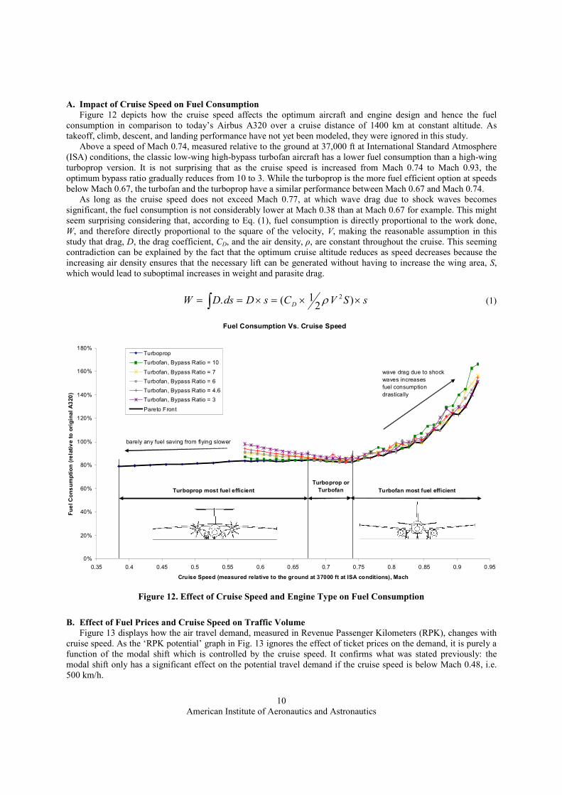
A. Impact of Cruise Speed on Fuel Consumption

Figure 12 depicts how the cruise speed affects the optimum aircraft and engine design and hence the fuel consumption in comparison to today’s Airbus A320 over a cruise distance of 1400 km at constant altitude. As takeoff, climb, descent, and landing performance have not yet been modeled, they were ignored in this study.

Above a speed of Mach 0.74, measured relative to the ground at 37,000 ft at International Standard Atmosphere (ISA) conditions, the classic low-wing high-bypass turbofan aircraft has a lower fuel consumption than a high-wing turboprop version. It is not surprising that as the cruise speed is increased from Mach 0.74 to Mach 0.93, the optimum bypass ratio gradually reduces from 10 to 3. While the turboprop is the more fuel efficient option at speeds below Mach 0.67, the turbofan and the turboprop have a similar performance between Mach 0.67 and Mach 0.74.

As long as the cruise speed does not exceed Mach 0.77, at which wave drag due to shock waves becomes significant, the fuel consumption is not considerably lower at Mach 0.38 than at Mach 0.67 for example. This might seem surprising considering that, according to Eq. (1), fuel consumption is directly proportional to the work done, W, and therefore directly proportional to the square of the velocity, V, making the reasonable assumption in this study that drag, D, the drag coefficient, CD, and the air density, ρ, are constant throughout the cruise. This seeming contradiction can be explained by the fact that the optimum cruise altitude reduces as speed decreases because the increasing air density ensures that the necessary lift can be generated without having to increase the wing area, S, which would lead to suboptimal increases in weight and parasite drag.

sSVCsDdsDW D ××=×== ∫ )21(. 2ρ (1)

B. Effect of Fuel Prices and Cruise Speed on Traffic Volume

Figure 13 displays how the air travel demand, measured in Revenue Passenger Kilometers (RPK), changes with cruise speed. As the ‘RPK potential’ graph in Fig. 13 ignores the effect of ticket prices on the demand, it is purely a function of the modal shift which is controlled by the cruise speed. It confirms what was stated previously: the modal shift only has a significant effect on the potential travel demand if the cruise speed is below Mach 0.48, i.e. 500 km/h.

Fuel Consumption Vs. Cruise Speed

0%

20%

40%

60%

80%

100%

120%

140%

160%

180%

0.35 0.4 0.45 0.5 0.55 0.6 0.65 0.7 0.75 0.8 0.85 0.9 0.95

Cruise Speed (measured relative to the ground at 37000 ft at ISA conditions), Mach

Fuel Consumption (relative to original A320)

.

Turboprop

Turbofan, Bypass Ratio = 10



Turbofan, Bypass Ratio = 4.6


Pareto Front

Turboprop most fuel efficient Turbofan most fuel efficient

Turboprop or

Turbofan

barely any fuel saving from flying slower

wave drag due to shock

waves increases

fuel consumption

drastically

Figure 12. Effect of Cruise Speed and Engine Type on Fuel Consumption


11

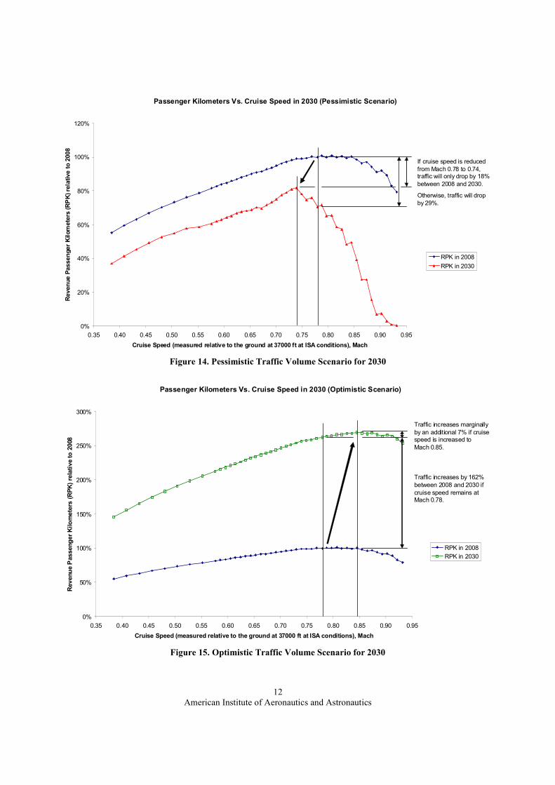
Using that graph as a baseline, the pessimistic and the optimistic traffic scenarios display how the traffic volume is affected by the fuel price as well as the cruise speed. Both graphs show that there is an optimum cruise speed at which the incentive to fly faster in order to utilize the aircraft more effectively balances the increase in fuel cost. The two scenarios assume the same oil and carbon prices as Section 1.E, i.e. $305/barrel and $180/metric ton CO2 in the pessimistic scenario and $55/barrel and $60/metric ton CO2 in the optimistic scenario. As these prices are more extreme than those assumed by EUROCONTROL in Table 1, it is not surprising that the traffic volume predictions in Fig. 13 are also more extreme: at the current A320’s cruise speed22 of Mach 0.78, the traffic multiplier reduces to 0.71 in the pessimistic scenario, but in the optimistic scenario it increases to 2.63.

If the cruise speed is reduced from Mach 0.78 to Mach 0.74 in the pessimistic scenario, Fig. 14 indicates that the

fuel saving outweighs the increase in the other operating costs. The overall cost reduction consequently ensures that the traffic only reduces by 18% instead of 29% in comparison to 2008. In the optimistic scenario, however, the low fuel and carbon prices lead to an operating cost saving if the cruise speed is increased to Mach 0.85. This way, Fig. 15 highlights that the traffic increases by an additional 7% in comparison to 2008.

Passenger Kilometers Vs. Cruise Speed in 2030 (Scenario Range)

0%

50%

100%

150%

200%

250%

300%

0.35 0.40 0.45 0.50 0.55 0.60 0.65 0.70 0.75 0.80 0.85 0.90 0.95


Revenue Passenger Kilometers (RPK) relative to 2008

RPK potential

pessimistic RPK

optimistic RPK

traffic volume

depends on fuel

price and cruise

speed

increase in traffic due to

reduced cost (fewer

aircraft)

RPK potential due to speed

(ignoring prices)

graph flattens off due to

rapidly rising fuel con-

sumption

increase in traffic due to

reduced cost (fewer

aircraft)

traffic reduces due to

rapidly rising fuel

consumption

Figure 13. Traffic Volume Scenario Range for 2030


12

Passenger Kilometers Vs. Cruise Speed in 2030 (Pessimistic Scenario)

0%

20%

40%

60%

80%

100%

120%

0.35 0.40 0.45 0.50 0.55 0.60 0.65 0.70 0.75 0.80 0.85 0.90 0.95



RPK in 2008

RPK in 2030

If cruise speed is reduced

from Mach 0.78 to 0.74, traffic will only drop by 18%

between 2008 and 2030.

Otherwise, traffic will drop

by 29%.

Figure 14. Pessimistic Traffic Volume Scenario for 2030

Passenger Kilometers Vs. Cruise Speed in 2030 (Optimistic Scenario)

0%

50%

100%

150%

200%

250%

300%

0.35 0.40 0.45 0.50 0.55 0.60 0.65 0.70 0.75 0.80 0.85 0.90 0.95



RPK in 2008

RPK in 2030

Traffic increases marginally

by an additional 7% if cruise speed is increased to

Mach 0.85.

Traffic increases by 162%

between 2008 and 2030 if

cruise speed remains atMach 0.78.

Figure 15. Optimistic Traffic Volume Scenario for 2030


13

C. Surplus Value Scenarios As the optimum design in terms of Surplus Value is not only affected by the cost function but also by the

revenue function, it is important to build a model that can not only predict the costs accurately, but also the revenue. Although there is a significant amount of uncertainty in forecasting aircraft operating costs in 2030, the predictabili-ty of revenue, and hence profit (i.e. Surplus Value), is even lower due to the underlying complexity in the airlines’ pricing strategies that depend on many factors, including the competitiveness in the market as well as the operating costs and the air travel demand.

The authors therefore assume that in 2030, the only constant will be the aim of the airlines to generate an operating margin of at least 10% as recommended by Ref. 25. Operating margin is defined in Eq. (2), and Eq. (3) shows how it can be used to calculate the operating profit (referred to as profit for simplicity) based on the costs. As Eq. (3) wrongly implies that high costs are beneficial because they lead to a higher profit, the model calculates the actual profit using Eq. (4). This latter formula assumes that one of the aircraft manufacturers will always offer an aircraft that is designed to fly at the optimum speed in terms of cost and that the airlines operating that aircraft will be able to price the tickets so that they can generate a 10% operating margin. As the other airlines will generally not be able to charge higher prices, their profit is equal to the fixed price minus their actual costs, as defined in Eq. (4).

operating margin = 10% = profit/revenue = (revenue – cost)/revenue (2)

profit = revenue – cost = 0.1 × revenue ⇒ revenue = cost/0.9 ⇒ profit = 0.1/0.9 × cost (3)

actual profit = minimum profit + minimum cost – actual cost = (0.1/0.9 + 1) × minimum cost – actual cost (4)

Figure 16 indicates that Eq. (4) generates the same optimum cruise speeds as Fig. 14 and Fig. 15. Apart from that, Fig. 16 highlights that a low fuel price gives the aircraft manufacturers and the airlines a larger margin of error in terms of cruise speed over which a profit can be generated, because a low fuel price has less of an impact on the total costs. Although the maximum traffic demand in the optimistic scenario is 3.3 times higher than in the pessimis-tic scenario, the maximum profit is slightly higher in the pessimistic scenario, surprisingly. This can be explained by the fact that the ticket prices in the pessimistic scenario are 3.4 times higher than in the optimistic scenario, which overcompensates for the lower demand.

Operating Profit Vs. Cruise Speed in 2030 (Scenario Range)

-300%

-200%

-100%

0%

100%

200%

300%

0.65 0.70 0.75 0.80 0.85 0.90 0.95

Cruise Speed*, Mach

Operating Profit relative to 2008

pessimistic RPK

optimistic RPK

- profit based on an operating profit margin of 10%, i.e. (1+0.1/0.9) x minimum cost achievable - actual cost

- speeds for maximum profit identical to speeds for minimum cost and maximum traffic

small margin of

error when fuel

prices are high

larger margin of error

when fuel prices are low

* measured relative to the ground

at 37000 ft at ISA conditions

Figure 16. Profit Scenario Range for 2030


14

D. Optimum Aircraft Designs

The designer can choose from an optimum turboprop as well as an optimum turbofan aircraft design for the pessimistic scenario’s ideal cruise speed of Mach 0.74, which are displayed in Fig. 17 and 18, respectively. The reason there are two optimum designs is because Fig. 12 shows that between Mach 0.67 and Mach 0.74 both the turboprop and the high-bypass turbofan have a similar fuel consumption at cruise conditions. The turboprop aircraft, represented by solid lines in Fig. 17, is based on the current Airbus A320 fuselage26, the Airbus A400M engines and wing fairing27, and the Avro RJ landing gear28. The turbofan aircraft, which is also represented by solid lines in Fig. 18, is entirely scaled off today’s A320, however. In both figures the dashed lines reflect the original dimensions. The comparison of the solid and the dashed lines shows that, due to the reduced cruise speed, both new designs have a greater wing span and less wing sweep than the current A320.

It might sound unrealistic that a future turboprop could fly at Mach 0.74, but today the A400M already cruises at an equivalent speed27. If the preliminary model was able to simulate takeoff and landing as well, it is likely that the turboprop aircraft would have a superior fuel efficiency because turboprops generally require less fuel to climb to their lower cruise altitudes in comparison to turbofan aircraft29.

a) Plan View

b) Front View

Figure 17. Turboprop Aircraft Optimized for a

Cruise Speed of Mach 0.74

a) Plan View

b) Front View

Figure 18. Turbofan Aircraft Optimized for a



15

In the optimistic scenario, the ideal cruise speed of Mach 0.85 produces the optimum turbofan aircraft design illustrated in Fig. 19. Unsurprisingly, the higher cruise speed leads to a higher wing sweep and a reduced wing span with respect to today’s A320.

V. Conclusion and Future Work

The fundamental question raised by this project and partially answered by the preliminary study presented in Section 4 is: Is there a business case to change the cruise

speed of today’s short-haul 150-seater aircraft and select

an advanced engine technology combination that

produces an engine design that is more robust to

uncertain fuel and carbon prices in 2030 than current

turbofans? As the entire aircraft design module is based on

preliminary design information and formulas, it cannot provide the model fidelty and accuracy achieved using Computational Fluid Dynamics codes or Finite Element Analysis models for example. Considering that future growth and fuel price scenarios are by definition educa-ted guesses, the precision gained by inserting higher fidelity codes into Fig. 4’s model framework is probably not worth the additional computational expense required.

Creating a Surplus Value formula that makes realistic profit predictions for 2030 is inherently difficult, as the preliminary study showed. Considering that the formula also produced the same optimum cruise speeds as the minimization of operating cost, it might be easier to focus on the latter metric. The pros and cons of the two metrics will be further investigated once the model envisaged in Fig. 4 has been completed.

Acknowledgments

The authors are very grateful for the intellectual contributions made by John Whurr, Alasdair Gardner, and Peter Swann at Rolls-Royce plc, a power systems provider. This project is funded by Rolls-Royce plc and the United Kingdom’s Engineering and Physical Sciences Research Council (EPSRC).

References 1Advisory Council for Aeronautics Research in Europe (ACARE), “Aeronautics and Air Transport: Beyond Vision 2020

(Towards 2050),” ACARE, 2010. 2Rolls-Royce, The Jet Engine, 6th ed., Rolls-Royce plc, London, 2005, pp. 266, 268, 275. 3Keane, A. J., Nair, P. B., Computational Approaches for Aerospace Design, 1st ed., John Wiley & Sons, Chichester, UK,

2005, Chaps. 1, 8. 4Sorrell, S., Speirs, J., Bentley, R., Brandt, A., Miller, R., “Global Oil Depletion,” United Kingdom Energy Research Centre

(UKERC), 2009. 5Airbus, “Global Market Forecast 2009-2028,” Airbus S.A.S., 2009. 6Donovan, S., Petrenas, B., Leyland, G., Caldwell, S., Barker, A., Chan, A., Dempsey, L., “Price Forecasts for Transport

Fuels and Other Delivered Energy Forms,” Auckland Regional Council, 2009. 7Committee on Climate Change (CCC), “Meeting the UK Aviation Target – Options for Reducing Emissions to 2050,” CCC,

2009. 8Rehrl, T., Friedrich, R., “Modelling Long-Term Oil Price and Extraction with a Hubbert Approach: The LOPEX Model,”

Energy Policy, Vol. 34, No. 15, 2006, pp. 2413-2428. 9United States Energy Information Administration (EIA), “Annual Energy Outlook 2010,” EIA, 2010.

a) Plan View

b) Front View

Figure 19. Turbofan Aircraft Optimized for a



16

10Anastasi, L., Dickinson, H., Kass, G., Smith, K., Stein, C., “Aviation and the Environment,” Parliamentary Office of Science and Technology (POST), 2003.

11Bower, C. G., Kroo, I. M., “Multi-Objective Aircraft Optimization for Minimum Cost and Emissions over Specific Route Networks,” International Congress of the Aeronautical Sciences (ICAS), AIAA, Reston, USA, 2008.

12Scheelhaase, J. D., Grimme, W. G., “Emissions Trading for International Aviation – An Estimation of the Economic Impact on Selected European Airlines,” Journal of Air Transport Management, Vol. 13, No. 5, 2007, pp. 253-263.

13Department for Transport (DfT), “The Future of Air Transport,” DfT, 2003. 14Van Hasselt, M., Van der Zwan, F., Ghijs, S., Santema, S., “Developing a Strategic Framework for an Airline Dealing with

the EU Emission Trading Scheme,” AIAA Aviation Technology, Integration and Operations Conference (ATIO), AIAA, Reston, USA, 2009.

15House of Commons Transport Committee, “The Future of Aviation,” House of Commons Transport Committee, 2009. 16Schimming, P., “Counter Rotating Fans – An Aircraft Propulsion for the Future,” Journal of Thermal Science, Vol. 12,

No. 2, 2003, pp. 97-103. 17Steffens, K., “Advanced Compressor Technology – Key Success Factor for Competitiveness in Modern Aero Engines,”

International Symposium on Air Breathing Engines (ISABE), AIAA, Reston, USA, 2001. 18Collopy, P. D., “Surplus Value in Propulsion System Design Optimization,” AIAA Paper, 97-3159, 1997. 19Raymer, D. P., Aircraft Design: A Conceptual Approach, 4th ed., American Institute of Aeronautics and Astronautics,

Reston, USA, 2006. 20Jenkinson, L. R., Simpkin, P., and Rhodes, D., Civil Jet Aircraft Design, 1st ed., Butterworth-Heinemann, Oxford, UK,

1999. 21Howe, D., Aircraft Conceptual Design Synthesis, 1st ed., Professional Engineering Publishing Limited, London, UK, 2000. 22Jackson, P. A., Jane’s All the World’s Aircraft 2006-2007, Jane’s Information Group Limited, Coulsdon, UK, 2006, pp.

262. 23Directorate-General for Mobility and Transport, “High-Speed Europe,” European Commission, 2010. 24EUROCONTROL, “Long-Term Forecast: IFR Flight Movements 2010-2030,” EUROCONTROL, 2010. 25Morrell, P. S. , Airline Finance, 3rd ed., Ashgate Publishing Ltd., Aldershot, UK, 2007, pp. 56. 26Airbus, A320 Airplane Characteristics for Airport Planning, Airbus S.A.S., Blagnac, France, 2005, p. 72. 27Jackson, P. A., Jane’s All the World’s Aircraft 2011-2012, Jane’s Information Group Limited, Coulsdon, UK, 2011, pp.

308. 28Jackson, P. A., Jane’s All the World’s Aircraft 1997-98, Jane’s Information Group Limited, Coulsdon, UK, 1997, pp. 528. 29Babikian, R., Lukachko, S. P., Waitz, I. A., “The Historical Fuel Efficiency Characteristics of Regional Aircraft from

Technological, Operational and Cost Perspectives,” Journal of Air Transport Management, Vol. 8, No. 6, 2002, pp.389-400.

strategic jet engine system design in light of …eprints.soton.ac.uk/196689/1/atio_paper.pdf ·...

Documents