Eindhoven, April 2016

by

R.C.M. Soetekouw

B.Sc. Industrial Engineering & Management Science Student Identity Number 0678784

in partial fulfilment of the requirements for the degree of

Master of Science in Operations Management and Logistics

Supervisors: dr. A. Chockalingam, TU/e, OPAC dr. S.S. Dabadghao, TU/e, OPAC R.J. Voster, KPMG, ITA FS S. Seijmonsbergen, KPMG, FRM

Economic capital for strategic risk in financial institutions

1

TUE. School of Industrial Engineering. Series Master Theses Operations Management and Logistics Subject headings: Strategic risk, Economic capital, Value at risk, Risk managements

2

Abstract

Strategic risk has caused failures during the latest financial crisis (Basel Committee on Banking Supervision, 2015); however, little is known about this risk type. We focus on the clarification of this subject by assessing the definition and the quantification of strategic risk. In this thesis, we discuss literature and legislation and use these insights to provide a comprehensive definition and model to quantify strategic risk. The definition is validated after conducting interviews with various experts in the field. The model is applied in a case study with public data from ABN AMRO. We compute the value at risk for strategic risk and compare it with the reported amount of strategic risk by the bank. We conclude that strategic risk can be quantified and that the model is a simple tool for banks to assess strategic risk. In addition, the model can be used by (small) banks in discussions with the supervisor. Furthermore, our findings can contribute to future regulation regarding strategic risk, since the current regulation regarding this topic lacks clear definitions and models.

3

Preface and acknowledgements

This report is the result of my master thesis commissioned by KPMG, which is the last requirement in the fulfillment of the master Operations Management and Logistics. I conducted this research with the guidance of many great people who I would like to thank explicitly in this word of gratitude.

I would like to thank Rob Voster from KPMG for guiding me in into the world of financial regulation and supporting me in all important decisions. Although the subject was risky to choose given the scarcity of literature and the contradictions in regulations and annual reports, you did not try to convince me of choosing a safe topic which I am very grateful for. After many doubts, the project turned out to be very interesting and that helped me to be motivated throughout the entire project. Furthermore, I would like to thanks Steven Seijmonsbergen for supporting me in the last two months of the project. I like the way you challenged me on the topic and the very detailed feedback you provided. Next to my supervisors at KPMG, I want to thank all my colleagues from the business units ITA FS and FRM. I had a great time and specially the ski trip will probably be an everlasting memory.

Many words of thanks to my supervisors at the TU/e dr. A. (Arun) Chockalingam and dr. S.S. (Shaunak) Dabadghao. I liked your openness towards the project and the way I could discuss my ideas with both of you. You provided me much freedom to come up with a creative solution and many guidance to conduct a proper research. I enjoyed working with both of you. Arun, thanks for supporting me throughout the project and all the time you spent to make this a success.

This master thesis is not only the end of my study, it is also the end of a wonderful time thanks to my fellow board members, all my friends, the rehousing committee and many more. I cannot even memorize all the activities and great moment I had with you. Thanks to all of you I have enough anecdotes to share for a very long time and I am sure that many more will follow.

I would also like to take the opportunity to thank my family. My brothers, for reminding me to graduate from the first day in college by asking “Aren’t you finished yet?” on a regular basis. And my parents for providing me the possibility to study and for supporting me in every possible way. Last but not least, Marloes thanks for always supporting me. We will have a great future together.

4

Executive summary

Background

Strategic risk, sometimes referred to as business risk, can be defined as the risk that earnings decline due to a changing business environment, for example new competitors or changing demand of customers. Threats from the business environment can seriously affect the profitability of banks and should therefore require significant attention from banks’ management and regulatory entities. Although qualitative assessment of strategic risk by management and supervisors is beginning to become common practice, a comprehensive definition and models to quantify this risk type could significantly contribute to better risk assessments and to literature.

Compared to credit risk, market risk, and operational risk, which are very standardized and well-researched risk types, strategic risk is underexposed. Currently, there does not exist a single definition of strategic risk in literature, legislation or in practice. Furthermore, literature on the topic is scarce and only a few theoretical models to quantify strategic risk exist.

Purpose

We aim to clarify the topic strategic risk by constructing a comprehensive definition and propose a model to quantify strategic risk. The objective is to gain more insight into this risk type that can help managers as a starting point in formalize them into governing processes, such as, frameworks and risk appetite limits; These insights can serve as a contribution to regulatory entities responsible for legislation and supervisors. Therefore, the following research questions are answered in the thesis.

The main question ‘Can economic capital for strategic risk be calculated?’

Sub question one ‘What is a quantifiable definition of strategic risk for financial institutions?’.

Sub question two ‘What is a suitable model to calculate economic capital for strategic risk?’.

Sub question three ‘Can these calculations help to set risk appetite limits in order to monitor strategic risk?’.

Method

This research uses the recommendations of Bertrand and Fransoo (2002) for operations management research. This model consist of four stages: conceptualization of the reality or problem, building a quantitative model, solving the model, followed by implementation. The conceptualization phase consists of a literature review and an in-depth analysis of definitions used by banks in practice. Furthermore, it assess regulatory documents to the use of strategic risk. The conceptualization phase ends with a definition for strategic risk, which is validated by experts in the field. The modelling phase introduces a model to quantify strategic risk. After this phase, the model is tested and used to obtain a solution for one particular case. The implementation is not part of this project.

5

Results

The first result is the answer on sub question one. After conducting extensive research in regulatory documents, literature and annual statements a definition was constructed and validated, by experts in the field with interviews. The definition is:

‘The risk of decline in net income due to unforeseeable changes in either revenues or fixed cost that are caused by external trends in the bank’s competitive environment or the extent to which the organization could timely adapt to these trends. These external trends in the competitive environment are: (one-of-a-kind) competitors, technology shift, customer priority shift, new-project failure, market stagnation, changes in regulation, industry margin squeeze and brand erosion. This risk increasingly extends beyond balance-sheet items to income generating activities, which are not attributable to position taking, credit losses or operational events. Income generating activities are: selling loans, origination, cash management, asset management, securities underwriting, payment services and client advisory services.’

Although all considered definitions, including this definition, overlap, this definition contributes in particular on two aspects. First, we established that strategic risk is the decline of net income. In other definitions, it was often defined as loss, volatility, or deviation from expectation. Second, it states a comprehensive range of external trend and events, in contrary to many definitions in which only some examples of external trends are mentioned.

Sub question 2 was answered by introducing a model to calculate economic capital for strategic risk. Without going into details in this summary, the model projects future net incomes on a strategy horizon of three years using a Brownian motion. In addition, a profitability limit was defined that serves as a threshold for the net income. The economic capital was then defined as the maximum of the limit minus the net income value and zero. By using simulation, a density function of the economic capital was obtained. Finally, strategic risk was expressed as the 99.95% upper limit of this distribution, also known as the value at risk. The results can be found in Figure 1.

The value at risk was first calculated for the case in which all parameters were assumed constant, this amount was 961 million. Second, an improvement to the model was made by allowing the profitability limit, in this case the absolute cost of equity, to increase over time. This resulted in a slightly higher value

0

200

400

600

800

1000

1200

Annual report Constant parameters Increasing COE

Economic capital

Figure 1 Results

6

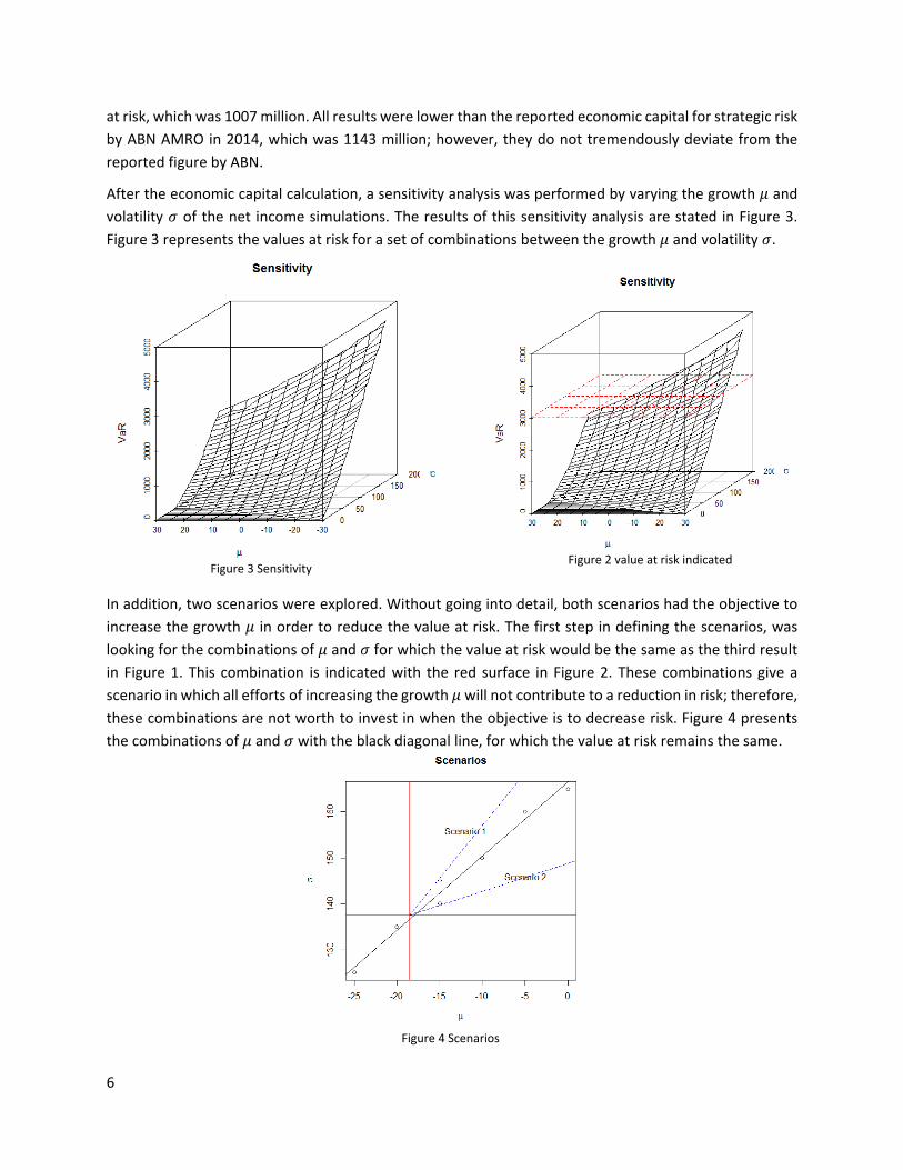
at risk, which was 1007 million. All results were lower than the reported economic capital for strategic risk by ABN AMRO in 2014, which was 1143 million; however, they do not tremendously deviate from the reported figure by ABN.

After the economic capital calculation, a sensitivity analysis was performed by varying the growth 𝜇𝜇 and volatility 𝜎𝜎 of the net income simulations. The results of this sensitivity analysis are stated in Figure 3. Figure 3 represents the values at risk for a set of combinations between the growth 𝜇𝜇 and volatility 𝜎𝜎.

In addition, two scenarios were explored. Without going into detail, both scenarios had the objective to increase the growth 𝜇𝜇 in order to reduce the value at risk. The first step in defining the scenarios, was looking for the combinations of 𝜇𝜇 and 𝜎𝜎 for which the value at risk would be the same as the third result in Figure 1. This combination is indicated with the red surface in Figure 2. These combinations give a scenario in which all efforts of increasing the growth 𝜇𝜇 will not contribute to a reduction in risk; therefore, these combinations are not worth to invest in when the objective is to decrease risk. Figure 4 presents the combinations of 𝜇𝜇 and 𝜎𝜎 with the black diagonal line, for which the value at risk remains the same.

Figure 2 value at risk indicated

Figure 3 Sensitivity

Figure 4 Scenarios

7

The cross point of the two red lines in Figure 4 indicate the values of the Brownian motion used in the second and third results of Figure 1. The objective was to increase 𝜇𝜇 from that point in order to decrease risk. It was assumed that the volatility would increase aswell since a change in strategy would increase the volatility of the income. In the first scenario, 𝜎𝜎 increased more rapidly than in the second scenario and they are separated by the combinations of 𝜇𝜇 and 𝜎𝜎 for which the value at risk would remain the same; this is all indicated in Figure 4.

The two scenarios generated some interesting results. The first scenario leads to an increase in the value at risk, while the second scenario leads to a decrease in the value at risk. Although the analysis is somewhat abstract, it showed how some strategies, even when growth is increased, will not help to decrease the amount of risk. These kinds of analysis could be used to set up frameworks for better decision making or to identify good or bad strategies. Even when it is impossible to get exact outcomes of these analyses, they can be very useful in providing qualitative insights to managers. These last results were gained to answer sub question 3. Although the results generated some useful insights that can be used for risk appetite limits of frameworks, it is worthwhile to note that the results do not provide strict limits to monitor strategic risk on an ongoing basis. Furthermore, it depends heavily on the data and the model assumptions. Therefore, hard objective monitoring cannot yet be done based on these simulations. However, more case studies might provide insight in the usefulness of this model when defining risk appetite limits.

Conclusion

Concluding, the model seems a surprisingly simple but effective tool to use in the assessment of strategic risk. So, to the best of our knowledge and based on the results of this thesis, the main question: ‘Can economic capital for strategic risk be calculated?’, can positively be confirmed.

8

Content

Abstract ......................................................................................................................................................... 2

Preface and acknowledgements ................................................................................................................... 3

Executive summary ....................................................................................................................................... 4

Content ......................................................................................................................................................... 8

Chapter 1: Introduction ........................................................................................................................ 10

Chapter 2: Research Questions ............................................................................................................. 13

2.1 Problem description .................................................................................................................... 13

2.2 Research questions ..................................................................................................................... 14

2.3 Research design .......................................................................................................................... 15

Chapter 3: Literature review ................................................................................................................. 16

3.1 Definition of strategic risk ........................................................................................................... 16

3.1.1 Definitions used in literature .................................................................................................. 16

3.1.2 Definitions used in practice .................................................................................................... 20

3.2 Definition of economic capital .................................................................................................... 22

3.3 Risk measures ............................................................................................................................. 25

Chapter 4: Definition of strategic risk ................................................................................................... 27

4.1 Interviews .................................................................................................................................... 27

4.2 Definition .................................................................................................................................... 29

Chapter 5: Modelling economic capital for strategic risk ..................................................................... 30

5.1 Introduction ................................................................................................................................ 30

5.2 Profitability limit ......................................................................................................................... 30

5.3 Stochastic process for net cash flows ......................................................................................... 32

5.3.1 Brownian motion with drift .................................................................................................... 33

5.3.2 The role of drift ....................................................................................................................... 33

5.3.3 Probability distribution of net cash flow ................................................................................. 33

5.3.4 Definition ................................................................................................................................ 34

5.3.5 Risk measure ........................................................................................................................... 34

Chapter 6: Simulation example ............................................................................................................. 36

6.1 Data ............................................................................................................................................. 36

9

6.1.1 Parameters for the Brownian motion ..................................................................................... 38

6.1.2 Estimating the Cost of Equity .................................................................................................. 39

6.2 Simulation ................................................................................................................................... 41

6.2.1 Simulation procedure ............................................................................................................. 41

6.2.2 Validation ................................................................................................................................ 42

6.3 Results ......................................................................................................................................... 43

6.4 Simulation accuracy .................................................................................................................... 46

6.5 Sensitivity .................................................................................................................................... 47

Chapter 7: Conclusion ........................................................................................................................... 54

7.1 Research conclusion .................................................................................................................... 54

7.2 Practical insights ......................................................................................................................... 55

7.3 Future research ........................................................................................................................... 55

7.4 Rigor and relevance .................................................................................................................... 56

Chapter 8: References .......................................................................................................................... 57

Chapter 9: List of abbreviations ............................................................................................................ 60

Chapter 10: Appendices .......................................................................................................................... 61

10

Chapter 1: Introduction

Considering the devastating effects of the latest financial crisis the overall objectives of this Regulation are to encourage economically useful banking activities that serve the general interest and to discourage unsustainable financial speculation without real added value. This implies a comprehensive reform of the ways savings are channelled into productive investments (European parliament, 2013a).

As can be seen in the citation above, the global financial crisis of 2007 was one of the main reasons to tighten the legislation for financial firms. Banks form a constant threat to the economy (European Parliament, 2013a), given the potential danger when they go bankrupt. Controlling risks and risk regulation are therefore major topics that have dominated financial institutions in the recent years.

Market risk, credit risk, and operational risk are by far the most well known risk types in regulation and literature. However, risk resulting from strategy and the business environment (e.g. competitors that enter the marker or changing customer demand) do not seem to get significant attention by regulation and literature. A new competitor entering the market can be a serious threat to the profitability of a bank; however, it is not required to hold capital buffers for strategic risk. Strategic risk can be defined as the risk that earnings decline due to a changing business environment, for example new competitors or changing demand of customers. It seems to be, more or less, the risk of being in business. So, can or should you mitigate against strategic risk at all? In the CAPM theory, volatility in earnings caused by the business environment is seen as firm specific risk. Firm specific risk can be neglected from a shareholders perspective, since shareholders can diversify this risk in their portfolio. So, why should banks be required to account for strategic risk when it is theoretically negligible from a shareholders perspective? This question can easily be answered with observations from the latest financial crisis. As the latest crisis revealed, when a bank defaults there is a large probability that they will be saved by governments with tax money. During the financial crisis, this was often indicated as ‘too big to fail’. ABN AMRO is one example of a bank that was acquired during the crisis by the Dutch government with tax money and will probably not generate a positive return on investment. Next to saving banks, governments interfere with financial institutions on other subjects; for instance, payment insurance or deposit guarantees (Berger, Hering, & Giorgio, 1995). This interference is referred to as the safety net by Berger et al. (1995). The society has every right to demand minimization of risk taking by banks, which includes risk resulting from the business environment, since taxpayers cannot diversify or interfere with business decisions as can shareholders. Regulators and authorities have a key role in protecting the society from risk taking by banks. This can be done by requiring banks to hold capital in order to mitigate against risk, as can be seen in following citation of the European Parliament:

Authorities are expected to impose higher own funds requirements on global systemically important institutions (G-SIIs) in order to compensate for the higher risk that G-SIIs represent for the financial system and the potential impact of their failure on taxpayers (European Parliament, 2013b).

Next to that, supervisors can even interfere with a bank’s management when necessary.

11

Since strategic risk has caused failures in the latest financial crisis (Basel Committee on Banking Supervision, 2015) it can be argued that strategic risk requires significant attention by banks’ management and regulatory entities. Although the business models and strategy are currently assessed by supervisors and have gain more weight in the latest regulations, the assessment is primarily done in a qualitative fashion and not quantified as credit risk, market risk, and operational risk are.

It can be stated that the risk resulting from the business environment on the profitability of a bank has increasingly gained more relevance since the 2007 crisis. Although in the past banks had little competition, the evolution in technology has opened the market for non-banking firms to participate in the banking industry by providing platforms and other services. These firms often do not need a banking permit but still have the ability to compete significantly with profitable activities of regular banks. This competition directly results in lower revenues and forces banks to lower prices resulting in thinner margins. Next to increasing competition, bank margins are already under tremendous pressure due to the low interest rates and the capital requirements that were introduced after the financial crisis. In a recent report, McKinsey&Company (2015) recognize the potential danger of non-banks attacking banking activities and they point out that the return on equity in the banking sector has not been above the cost of equity since the latest financial crisis. This report indicates that the banking industry struggles to stay profitable under the current business environment.

Taking all these developments into account, it can be concluded that banks operate in a more dynamic business environment than before, resulting in the need to better understand strategic risk, and specially the size of it. When future revenues of banks are threatened by strategic risk, mitigation with capital might be a necessity. Moreover, even when mitigation with capital buffers is not desirable, it might be very useful to have an idea of the size of strategic risk and how it differs among firms. This could help banks to benchmark their strategic risk in relation to competitors. Furthermore, having an idea of the size can help to set risk appetite limits to objectively control strategic risk, which can be an effective way to mitigate against risk. Risk appetite limits are widely used as a method to control risk and therefore mitigate against unwanted effects. Although most annual report use the term risk appetite intuitively without proper definition, Deutsche bank (2016) provides a clear definition:

‘Risk appetite expresses the level of risk that we are willing to assume within our risk capacity in order to achieve our business objectives, as defined by a set of minimum quantitative metrics and qualitative standards (Deutsche Bank, 2016).’

Risk appetite limits for strategic risk seems to be a challenge since it contains many qualitative aspects and quantification of this risk type is considered hard. Therefore, more research into quantification of strategic risk can contribute to define risk appetite limits and can help to set or support qualitative standards. These limits, when they can be defined, will eventually help to mitigate against the unwanted effects of strategic risk.

Concluding, there is a need for models to quantify strategic risk. First, quantification of strategic risk could help a board of directors to assess their current business models and make a comparison to other types of risks. In addition, quantifying strategic risk could help to set risk limits in order to take corrective actions when needed. Second, banks can be forced by their supervisors to retain additional own funds to cover for strategic risk (European Banking Authority, 2014). However, supervisors do not have models to

12

calculate strategic risk which makes the required amount of additional own funds arbitrary. Third, literature regarding strategic risk and specially the quantification of it is scarce. Research on quantitative models to calculate strategic risk would significantly contribute to literature.

The rest of the thesis will be structured as follows. Chapter 2 will provide the problem description and will address the relevance of this research in more detail. Next to the problem description, the main and sub question are presented followed by the research design. Roughly the research will cover two aspects of strategic risk, which are issues regarding the definition and a quantitative model to calculate strategic risk.

After the research questions and design, the literature review in chapter 3 will provide sufficient background information needed throughout the thesis in order to answer the research questions. Chapter 3 will first address the definition of strategic risk in literature and in practice. In addition, the concept of economic capital will be introduced in which risks are often expressed.

Part of the research design in chapter 2 is an interview regarding the definition of strategic risk. As already mentioned, literature on strategic risk is scarce resulting in a wide variety of definitions in literature and in practice. Chapter 4 presents the results of this interview regarding the definition of strategic risk and will propose a detailed definition on which the quantitative model can be based.

Chapter 5 elaborates on the model to calculate strategic risk. The model will be based on the definition obtained in chapter 4 and will be built up systematically.

After the model has been defined, chapter 6 will provide a simulation example including a sensitivity analysis. The example will be based on public data of ABN AMRO. Followed by the conclusion in chapter 7. In which an extensive conclusion and recommendations for future research will be provided.

13

Chapter 2: Research Questions

2.1 Problem description

As stated in chapter 1, banks are currently more exposed to strategic risk. According to the BCBS (2015) strategic risk and non-viable business models have shown to cause failures during the financial crisis from 2007 to 2009, which emphasize the need to understand and control strategic risk. To contribute to a better understanding of strategic risk there are two main issues that have to be addressed; that are the definition and the quantification of strategic risk. Since many parts of the thesis will refer to legislation, Appendix A provides a short overview of regulatory entities.

First, strategic risk has a wide variety of definitions in literature and in practice. Literature is scarce and does not provide consistency. The annual statements of most banks report on strategic risk and provide the definition that they use; however, these definitions differ significantly. When comparing the definitions among banks and in literature, it becomes clear that a single comprehensive definition could contribute to a better understanding of this risk type.

Second, a good model would definitely contribute to a more accurate estimation of strategic risk. Many banks include strategic risk in the economic capital in addition to credit risk, market risk, and operational risk; however, models to support these measures of economic capital for strategic risk are lacking. Economic capital is a measure of risk exposure often used by banks to express the amount of risk at exposure. Next to banks, supervisors will also profit from a good model for strategic risk. Currently, supervisors assess banks on strategic risk with business model analysis (European Banking Authority, 2014). Business model analysis (BMA) is part of the procedures and methodologies for the supervisory review and evaluation process. The supervisory review and evaluation process (SREP) provides guidelines to supervisors of how they should conduct the BMA. The BMA assess two main questions regarding strategic and business risk by grading them on a scale from 1 (no risk) to 4 (high risk). First, the viability of the business model to generate admissible returns in a 12 month period is assessed by the supervisor. Second, supervisors must assess the sustainability of the strategy on being able to generate admissible returns on a 3-year forward-looking period based on the strategic plans and financial forecast. However, the criteria for admissible returns, viability and sustainability are mostly qualitative; apart from some performance metrics. Without a proper method to quantify strategic risk, it will be difficult to compare institutions on an equal base since there is no single metric supported by a model that estimates or expresses the size of strategic risk. So, regulatory entities could also benefit from a model that quantifies strategic risk because it makes the BMA less qualitative and it will allow for an equal assessment among banks. Literature only provides a few papers that discuss models for strategic risk. More research on this topic will contribute to a more extensive perception on strategic risk.

Summarizing, threats from the business environment can seriously affect the profitability of banks and should therefore require significant attention from banks’ management and regulatory entities. Although qualitative assessment of strategic risk by management and supervisors is beginning to become common

14

practice, a comprehensive definition and models to quantify this risk type could significantly contribute to better assessments and to literature.

2.2 Research questions

To assess the size and to get managerial insights on the relevance of strategic risk, a quantitative risk assessment should be in place. Therefore, strategic risk should be captured in the economic capital as it is also recognized by the Basel Committee on Banking Supervision (2009) and done in practice by many banks. Although the relevance of strategic risk seems to be accepted by banks and regulatory institutions, the definition is still unclear as are the underlying quantification models. Therefore, the main research question is:

Main research question:

Can economic capital for strategic risk be calculated?

The first question that must be addressed is ‘What is the definition of strategic risk?’. There are many definitions available in literature and provided in annual statements and in legislation. Most of them have some overlap; some of them are very short, while others include a more in-depth explanation of strategic risk. Nevertheless, a single industry standard should be the ultimate goal. Furthermore, in order to model strategic risk a proper definition should be formed to support the model. The first sub- question is therefore:

Sub question 1:

What is a quantifiable definition of strategic risk for financial institutions?

After the definition is set, a suitable model must be developed that can calculate economic capital for strategic risk. When a model can be defined, this will lead to a major step in answering the main question. Although literature on this topic is scarce, when the definition is properly set we might succeed in modelling strategic risk by combining different models from literature or legislation. The second sub question that must be addressed to answer the main question can be found below. Typical topics that should be addressed to answer this question are: What are the input parameters and variables? What is a suitable model? Which aspects of strategic risk are material? Which strategic events have to be included? And of course, the model must be validated. Furthermore, the model must be applied on a case study to confirm its usefulness and to test whether it provides reasonable outcomes.

Sub question 2:

What is a suitable model to calculate economic capital for strategic risk?

The model obtained from sub question 2 can be used to calculate the magnitude of strategic risk. Insights into the size of this risk type can help to set risk appetite limits to control strategic risk. These risk appetite limits form the core of the last research sub question. Risk appetite limits are essential when governing strategic risk. If strategic risk can be properly calculated, these insights can be formalized into frameworks

15

that define a tolerable limit to which a bank is willing to accept risk and a non-tolerable limit. The last research question will explore whether the model can be used to define risk appetite limits.

Sub question 3:

Can these calculations help to set risk appetite limits in order to monitor strategic risk?

2.3 Research design

The research design will follow the recommendations of Bertrand and Fransoo (2002) for operations management research, which is indicated in Figure 5. This model consist of four stages: conceptualization of the reality or problem, building a quantitative model, solving the model, followed by implementation. This thesis will assess all research question by following these steps.

Figure 5 Research model (Bertrand & Fransoo, 2002)

The conceptualization phase will consist of a literature review and an in-depth analysis of definitions used by banks in practice. Furthermore, it will assess regulatory documents to the use of strategic risk. The conceptualization phase will end with a definition for strategic risk, which will be validated by experts in the field. The modelling phase will introduce a model to quantify strategic risk. After this phase, the model is tested and used to obtain a solution for one particular case. The implementation will not be part of this project.

16

Chapter 3: Literature review

The literature section will elaborate on three topics, which are: the definition of strategic risk, the definition of economic capital, and risk measures. As already stated in section 2.2, there are many definitions regarding strategic risk in literature and in practice. Some use the term business risk instead of strategic risk and the content of the same definitions differ significant across literature and in practice. To address the inconsistency and to answer sub question 1, section 3.1 will provide an overview of definitions in literature and in annual statements. After the definition of strategic risk has been set, section 3.2 will elaborate on the definition of economic capital. This section will provide an overview of definitions used by banks and will elaborate on the importance of economic capital in the risk assessment process. Last, section 5.3.5 will state the most commonly used risk measures to express risks, which are crucial to answer sub question two, three and the main research question.

3.1 Definition of strategic risk

The terms business risk and strategic risk are used interchangeably across literature and in practice and the content of the definitions is often the same. Therefore, both terms were taken into consideration during the literature review to obtain a full scope of definitions. This section starts with the definitions in academic literature and in regulatory documents. Next, the definitions in annual statements are provided followed by a complete definition validated by the interviews.

3.1.1 Definitions used in literature

Before presenting the relevant literature on strategic risk, it is important to consider how strategic risk relates to credit risk, market risk, and operational risk. In order to indicate the difference, losses are divided into assets losses and income losses. An overview is presented in Table 1.

Risk type

Loss

type

Credit Risk Market risk

Strategic risk Operational risk

Assets

Income Table 1 classifications of risk types

As can be seen in Table 1, credit and market risk are related to asset losses; such as, losses on loans and on positions in the market. Whereas strategic risk and operational risk are related to decline of income due to strategic or operational events; such as, losses that affect the profit and loss statement due to fraud in the case of operational risk or losses due to a disruptive competitor in the case of strategic risk.

17

The first classification given by Schroeck (2002) places business risk in a broad perspective, which can be seen in the schematic overview in Figure 6. In this framework, business risk and event risk are part of operational risk. Schroeck (2002) defines operational risk as:

The risk of experiencing unexpected (financial) losses due to failures in people, processes or systems and their (internal) controls or from external (nonmarket or non-credit-risk) events and a bank’s business strategy/business environment. These risks are common to all companies, not just banks, and can lead to a bank’s default at any time between now (t = 0) and a predetermined period of time ending at time horizon H. (Schroeck, 2002)

The definition of operational risk used by Schroeck (2002) differs from the definition of operational risk as it is currently used in banks. To be more specific, operational risk as it is known nowadays equals the event risk in the classification of Schroeck (2002) in Figure 6.

Business risk in Figure 6 is defined as the loss of unforeseeable changes in either revenues or fixed cost that are caused by changes in the bank’s competitive environment. These changes in the competitive environment are for example, price wars, new market entrants or changes in regulation.

Schroeck (2002) defines event risk as losses due to processes failures, systems failures, fraud, legal claims or external disruptions that are caused by a rare event. Which is in essence the definition for operational risk (Basel Committee on Banking Supervision, 2006; Basel Committee on Banking Supervision, 2009; European Parliament, 2013a; Sweeting, 2011).

Figure 6 Overview of operational risk according to Schroeck (2002)

It should be mentioned that the European Parliament (2013a) does not include external events resulting from strategic risk in operational risk. So in essence, they only use half the definition of operational risk from Schroeck (2002). The Basel Committee on Banking Supervision (2011) even explicitly exclude strategic risk from operational risk:

Operational risk is defined as the risk of loss resulting from inadequate or failed internal processes, people and systems or from external events. This definition includes legal risk, but excludes strategic and reputational risk. (Basel Committee on Banking Supervision, 2011)

Although the European Parliament (2013a) does not include the events from business risk in operational risk, the definition of Schroeck (2002) seems more comprehensive since external business or strategic

Operational risk

Event risk Business risk

18

events can have large effects as well. Concluding, the classification in Figure 6 can be very useful when analyzing strategic risk. It implies an overlap between operational risk and business risk/strategic risk. Since more research is conducted on operational risk, some of these findings or models might be useful when analyzing strategic risk.

The next definition is provided by the Basel Committee On banking Supervision (2009):

Business risk is more clearly defined as the risk that volumes may decline or margins may shrink, with no opportunity to offset the revenue declines with a reduction in costs. For example, business risk measures the risk that a business may lose value because its customers sharply curtail their activities during a market down-turn or because a new entrant takes market share away from the bank. Moreover, this risk increasingly extends beyond balance-sheet items to fee-generating services, such as origination, cash management, asset management, securities underwriting and client advisory services.

This definition is used in the economic capital framework that is proposed by the BCBS (2009). First, this definitions states that strategic risk has an effect on the profit and loss statement since it addresses declines in revenues, which is amplified later on by stating that strategic risk extends beyond balance sheet items. This differs from market and credit risk that focus only on the balance sheet. For instance, credit risk is obviously related to balance sheet items like loans. A defaulting loan will affect the balance sheet because chances are high that deductions on the loan have to be made. Strategic risk, however, affects future income. For instance, when customer needs are changing this will result in lower volumes and might cause reduced income in a particular year. So, strategic risk needs a forward-looking approach and depends on future cash flows. The definition of the BCBS (2009) further states two examples of strategic risks, which are changing customer activities and the entrance of a competitor. This definition, however, does not include a wide range of external events apart from some examples. A comprehensive set of external events can be found in the following definition of Slywotzky & Drzik (2005).

A broad risk governance framework, which breaks down strategic risk in workable determinants, is proposed by Slywotzky & Drzik (2005). Slywotzky & Drzik (2005) define strategic risk as the risk of external trends or events that can influence a company’s growth or value (Slywotzky & Drzik, 2005). The external trends or events are the determinants of strategic risk and are covered by: Industry margin squeeze, technology shift, brand erosion, one-of-a-kind competitor, customer priority shift, new-project failure, and market stagnation. The framework to address these trends and events is built on the steps presented in Figure 7.

19

Figure 7 strategic risk management framework (Slywotzky & Drzik, 2005)

Doff (2008) attempts to provide a definition for the term business risk and identifies whether business risk can be calculated within an economic capital framework. Doff (2008) focusses on addressing business risk in a banking environment and answers the question in which situations economic capital is a suitable solution to absorb losses caused by strategic/business risk. Doff (2008) defines business risk as:

The risk of financial loss due to changes in the competitive environment or the extent to which the organization could timely adapt to these changes (Doff, 2008).

Two determinants; ‘adaption to changes’ and ‘competitive environment’ from the above definition are used by Doff (2008) to classify different combinations of adaption and environment into: low, medium or high business risk. Table 2 provides the result of this classification.

Internal organization

Com

petit

ive

En

viro

nmen

t

Adapt quickly Adapt slowly

Dynamic Business risk Medium

Business risk High

Stable Business risk Low

Business risk Medium

Table 2 Components of business risk (Doff, 2008)

Furthermore, Doff (2008) distinguishes two components of changes in the competitive environment. First, changes can occur abrupt or gradually. Second, changes may be permanent or temporally. The author argues that only the combination ‘abrupt temporary changes’ and ‘abrupt permanent changes’ are worthwhile to mitigate with an economic capital buffer. There is no use in mitigate the other two combinations with an economic capital buffer. The logic behind this claim is intuitively simple. When changes occur gradually, it is better to adapt the organization. Doff (2008) therefore concludes that economic capital can be used to absorb loss in the following situations:

• A short crisis in case of an abrupt temporary change • The time lag between an event and successful management interaction • The initial investment of a change in the organizations and other unavoidable costs

1. Identify and assess strategic

events and trends

2. Map risks

3. Quantify risks

4. Identify the potential

upside

5. Develop mitigation

action plans

20

Doff (2008) provides a graphical representation of the loss that must be absorbed and the structure of revenue evolution after a strategic event. This graphical representation can be found in Figure 8.

Figure 8 Revenue evolution after a strategic event Doff (2008)

It can be derived from all the definitions mentioned in this section that strategic events affects the profit and loss statement and that the absence or delay of a good strategy to offset the business change can cause declining revenues or even loss.

3.1.2 Definitions used in practice

In addition to the literature, eight banks that operate in the Netherlands were examined on reporting on strategic risk in the annual reports. These banks include: ABN Amro, ING, Binckbank, Deutche Bank, Rabobank, Van Lanschot, SNS, and RBS. The reports are all publicly available and reporting on the fiscal year 2014. In every annual report the words ”business risk” and “strategic risk” was searched and the corresponding definition was documented. Furthermore, the economic capital amount, when provided for strategic/business risk in the annual report, was included in an overview. Table 10, Table 11, Table 12 show the results of these findings and are stated in Appendix C.

Table 10 displays the use of the term business risk. As can be seen, four banks use the term business risk and three of these banks allocated economic capital to mitigate against its effects. It is worthwhile to note that Binckbank does not allocate economic capital to business risk; however, Binckbank does spend a significant amount of attention to business risk in the annual report. Binckbank, which is mostly known for providing an online approachable trading platform to consumers, operates within a highly competitive market niche. Their income heavily depends on transaction fees. From the total net income of 132,321 million euros in 2014, 79,631 million euros was generated from transaction fees. It can be stated that the activities of Binckbank are not very diversified making it vulnerable for competitors and changing consumer preferences. The following citation from the annual report stresses this statement:

21

‘The executive board considers that business risk (earnings volatility) is too high, since BinckBank is still too dependent on income from securities transactions. Over the longer term therefore, BinckBank wishes to create a more stable earnings flow and to become less dependent on transaction-related income. (…) The desired risk profile for business risk has therefore not been realised. (Binckbank, 2014)’

Although Binckbank does not allocate economic capital to business risk, it recognize the potential danger of the risk and the material impact. One example from Table 10 that does allocate economic capital to business risk is Deutsche Bank. As can be seen in Table 10, in total 3,084 billion euros was allocated to their economic capital to cover business risk. It is claimed by Deutsche bank that the most material part of business risk is strategic risk as can be seen in following citation:

‘The most material aspect of business risk is ‘strategic risk’, which represents the risk of suffering unexpected operating losses due to decreases in operating revenues which cannot be compensated by cost reductions within the respective time horizon. (Deutsche Bank, 2014)’

This statement of the Deutsche Bank corresponds with the definition of ING, which also explicitly mention the inclusion of strategic risk in the business risk definition.

ABN AMRO does not mention strategic risk as part of business risk. However, the description: ‘(…) the risk that earnings will fall below the fixed cost base, due to changes in margins and volumes’, more or less equals the strategic risk definition of Deutsche Bank and ING. It can therefore be argued that the definition of business risk equals the definition of strategic risk used by Deutsche bank and ING.

RBS uses business risk more as a collection of different external risk types as can be seen in the definition. However, RBS does disclose strategic risk separately which is discussed later on in Table 12.

Table 11 shows the annual report in which the term strategic risk is used. It can be derived from Table 11 that two out of three banks, which are SNS and RBS, do not allocate economic capital to strategic risk. Van Lanschot does allocate economic capital. As can be seen in the description of strategic risk at Van Lanschot, the term business risk is sometimes used to indicate strategic risk. It can be stated that both terms have the same meaning in the annual report of Van Lanschot; taking into account that Van Lanschot did not give a separate explanation of the term business risk as it did for strategic risk, and given the context in which the term business risk was used, The three banks in Table 11 use in essence the same definition. Generally, it includes the components: late anticipation on future changes in environment, and incorrect strategic decisions.

The last table shows the use of strategic and/or business risk as part of operational risk. As can be seen in Table 12, NIBC introduces a new term “strategic business risk”. Rabobank does mention it in the report next to operational risk, but does not give a definition in the report. It is worthwhile to note that Table 12 does not report on the economic capital amounts, because the annual statements mix it with operational risk and therefore do not provide an objective measurement.

It should be noted that the literature often refers to loss as strategic risk; however, some of the definitions used by banks in Appendix C are more subtle. The citations below indicate that with the terms: ‘decline in

22

earnings’, ‘lower income’, and ‘deviate from expectations’. This suggests that considering only losses as strategic risk might be an underestimation.

‘The risk that business earnings and franchise value decline and/or deviate from expectations’ (ABN AMRO,2014)

‘Strategic risk is the risk of lower income due to a change in the bank’s environment and its activities.’ (Van Lanschot, 2014)

The issue whether to consider loss or deviations/declines in income is addressed in the interviews since it is of vital information in a quantifiable definition. This topic will be addressed in the next section.

Concluding, it seems obvious that there is not one single definition among banks regarding strategic risk. In some cases, strategic risk is treated as part of business risk and in other cases strategic risk is treated as a standalone risk. Furthermore, it can be stated that not every bank allocates economic capital to business risk or strategic risk; however, when economic capital is allocated, it is mostly allocated to strategic risk. Strategic risk is predominantly seen as material by banks. Regarding the economic capital allocation for business risk and strategic risk, most banks do provide a definition of the measurement; however, none of them disclose usable models in their reports. It is therefore hard to benchmark the different definitions and the economic capital levels for an outsider. More information is needed to objectively compare banks. Although not emphasized in the definitions stated above, most banks have governance structures and have defined risk appetite levels to monitor and evaluate business and/or strategic risks. This is important to note because this indicates that next to the quantitative economic capital measure, banks also qualitatively assess business and strategic risk.

3.2 Definition of economic capital

Economic capital has many definitions in literature. Sweeting (2011) states that economic capital refers to a surplus of assets or cash flows to deal with an unforeseeable decrease in assets or rise in liabilities over a predefined period within specific risk limits. The Bank of International Settlements (2009) defines economic capital as procedures or routines of banks to evaluate risk and cover the financial impact due to banks risky activities. The definition of the Bank of International Settlements (2009) differs from the definition of Sweeting (2011) in a way that economic capital can be seen as a banks’ measurement of overall risk or risk across business units and not as a capital buffer. Economic capital in the context of a banks risk management is not a mandatory capital buffer as is the regulatory capital under pillar 1 of the Basel framework.

In practice, there is not a single methodology for banks to assess the economic capital; therefore, banks use different internal models and processes in their internal risk assessment (K. Aas, G.Puccetti, 2014). The concept, however, is the same across banks:

ING BANK (2014) - EC is defined as the amount of capital that a transaction or business unit requires in order to support the economic risks it takes. In general, EC is measured as the unexpected loss above the expected loss at a given confidence level

23

ABN AMRO (2014) – Economic capital is the amount of capital ABN AMRO needs to hold in order to achieve a sufficient level of protection against large unexpected losses that could result from extreme market conditions or events.

DEUTSCHE BANK (2014)- Economic capital measures the amount of capital we need to absorb very severe unexpected losses arising from our exposures. “Very severe” in this context means that economic capital is set at a level to cover with a probability of 99.98 % the aggregated unexpected losses within one year. We calculate economic capital for credit risk, for market risk including trading default risk, for operational risk and for business risk. RABOBANK (2014) - Economic capital refers to the minimum capital buffer required in order to offset all unexpected losses caused by the various risks to which a bank is exposed during a specific time period (one year), assuming a specific reliability interval.

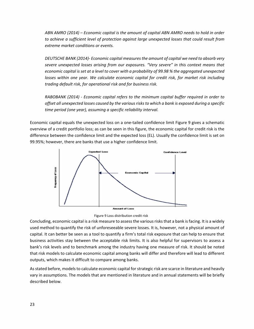
Economic capital equals the unexpected loss on a one-tailed confidence limit Figure 9 gives a schematic overview of a credit portfolio loss; as can be seen in this figure, the economic capital for credit risk is the difference between the confidence limit and the expected loss (EL). Usually the confidence limit is set on 99.95%; however, there are banks that use a higher confidence limit.

Concluding, economic capital is a risk measure to assess the various risks that a bank is facing. It is a widely used method to quantify the risk of unforeseeable severe losses. It is, however, not a physical amount of capital. It can better be seen as a tool to quantify a firm’s total risk exposure that can help to ensure that business activities stay between the acceptable risk limits. It is also helpful for supervisors to assess a bank’s risk levels and to benchmark among the industry having one measure of risk. It should be noted that risk models to calculate economic capital among banks will differ and therefore will lead to different outputs, which makes it difficult to compare among banks.

As stated before, models to calculate economic capital for strategic risk are scarce in literature and heavily vary in assumptions. The models that are mentioned in literature and in annual statements will be briefly described below.

Figure 9 Loss distribution credit risk

24

• At the moment, there are no regulations or guidelines from regulatory entities that addresses the quantification of strategic risk. Although the Basel Committee on Banking Supervision (2009) argues that strategic risk should be part of the economic capital assessment, it does not provide any guidelines to quantify it.

• Doff (2008) reports three commonly used methods to calculate the economic capital for strategic risk: Analogue company approach/peer group analysis, statistical analysis and scenario analysis. These methods are not funded on literature but rather on his own experience with banks.

• Schroek (2002) proposed two methods to calculate the economic capital for business risk, which are:

historical accounting based-Approach and Monte Carlo Simulation. The first one uses historical cost and revenue time series in which all trading and credit related cost and revenues are subtracted. These figures can then be used to calculate the expected revenue and the sigma of volatility after which the economic capital for business risk can be calculated. The second approach, Monte Carlo simulation, also depends on historical data. It does, however, not depend on adjusted profit and loss data. Schroeck (2002) proposed that the Monte Carlo simulation could be done by linking the drivers to a suitable macro-economic model. It should be noted that the last model is only abstractly described by the author. Lastly, Schroeck (2002) argues that economic capital can be modelled at a corporate level or at a business-line level. The last one should include correlations to consider the diversification benefits.

• A more detailed model can be obtained by calculating the discounted cash flows in a continuous time model (Böcker, 2008). Böcker (2008) projects discounted future cash flows by using Brownian Motions to calculate the capital at risk (CaR).

• Chaffai et al. (2015) use a directional distance function to calculate the difference between the current profit and an efficient frontier. The difference is considered as profit inefficiency, which they see as unexpected loss. Business risk is defined here as changes in profit due to a bank’s activities.

• Last, the ABN AMRO bank mentioned their method briefly in the annual statement, which can be seen

in following citation: ‘Economic capital for business risk is defined as the maximum downward deviation of net operating profit from the expected net operating profit.’ (ABN AMRO, 2014)

As can be seen, the models differ highly in approach. Furthermore, it is worthwhile to note that most models in literature only consider losses (negative income) as part of economic capital, while annual statements often refer to loss as deviation from expectation or budgets. Next to ABN AMRO in the citation above, Deutsche Banks (2016) defined in their latest report: ´Strategic Risk is the risk of a potential earnings downside due to revenues and/or costs underperforming plan targets’ (Deutsche Bank, 2016).

Whether negative earnings or deviation from budget should be used is not clear from literature. Chapter 4 will elaborate on this topic by addressing it in the interviews.

25

3.3 Risk measures

Quantification is one of the most challenging aspects of risks. Risk measures should be used to calculate the amount economic capital and to internally assess the effects or magnitude of risk types (Basel Committee on Banking Supervision, 2009). To be more concrete, considering Figure 9 and the economic capital for credit risk. The idea of economic capital is in this case straightforward; it is the difference between the expected and the upper limit of the distribution. The question that remains is: ‘How to set this limit?’. This section will present various measures to answer this question.

There are many standard risk measures and derivations of these risk measures discussed in literature and used in practice. Before presenting the most commonly used risk measures, it is important to note that the BCBS (2009) provides characteristics to which a risk measure should comply. These characteristics are:

1. Intuitive, there should be a clear intuition of a risk measure.

2. Stable, Small changes in the model parameters or in the assumptions of the model should not lead to

large changes in a risk measure.

3. Easy to compute, calculations of a risk measures are preferably easy. Complexity should weigh against

the cost.

4. Easy to understand, management should no wat the risk measures mean.

5. Simple and meaningful risk decomposition, risk should simple to be decomposed to business lines or

individual exposures.

6. Coherent:

a) Monotonicity: 𝑋𝑋,𝑌𝑌 ∈ 𝑉𝑉,𝑌𝑌 ≥ 𝑋𝑋 → 𝜌𝜌(𝑌𝑌) ≤ 𝜌𝜌(𝑋𝑋)

The monotonicity axiom states that if a portfolio Y drawn from the same set of random values V as portfolio X, always has at least a higher value than X, The risk of X cannot be higher than the risk of Y.

b) Positive homogeneity: 𝑋𝑋 ∈ 𝑉𝑉, ℎ > 0, ℎ𝑋𝑋 ∈ 𝑉𝑉, 𝜌𝜌(ℎ𝑋𝑋) = ℎ𝜌𝜌(𝑋𝑋)

When exposures are multiplied with a factor, the risk measure is multiplied with that same factor.

c) Translation invariance: 𝑋𝑋 ∈ 𝑉𝑉,𝑎𝑎 ∈ ℝ, 𝜌𝜌(𝑋𝑋 + 𝑎𝑎) = 𝜌𝜌(𝑋𝑋) − 𝑎𝑎

If a risk free asset is included in a portfolio, the risk measure should decline with the same amount.

d) Subadditivity: 𝑋𝑋,𝑌𝑌,𝑋𝑋 + 𝑌𝑌 ∈ 𝑉𝑉 → 𝜌𝜌(𝑋𝑋 + 𝑌𝑌) ≤ 𝜌𝜌(𝑋𝑋) + 𝜌𝜌(𝑌𝑌)

The risk measure of two combined portfolios is always smaller than the separate sum of both portfolios, this reflects the diversification of risk.

26

There are a number of well-known risk measures to calculate economic capital. The Basel Committee on banking supervision defines standard deviation, value at risk, expected shortfall, spectral risk measures, and distortion risk measures. A clarification per risk type will be provided below:

The first risk measure is standard deviation. This risk measure is, for instance, used in the mean-variance theory (Guégan & Hassini, 2015). This risk measure, however, assumes symmetrical return distribution, which is hardly true in practice (Guégan & Hassini, 2015). Next to that, standard deviation as a risk measure is not coherent because it violates the monotonicity constraint (Basel Committee on Banking Supervision, 2009).

The second risk measure, value at risk 𝑉𝑉𝑎𝑎𝑅𝑅𝛼𝛼, is widely used in practice and represents a confidence interval of the loss distribution. The 𝑉𝑉𝑎𝑎𝑅𝑅𝛼𝛼 put all the weight on the 𝛼𝛼-quantile (Dowd, Cotter, & Sorwar, 2008). The value at risk can be represented by (Guégan & Hassini, 2015):

𝑉𝑉𝑎𝑎𝑅𝑅𝛼𝛼(𝑋𝑋) = inf{𝑥𝑥|𝑃𝑃[𝑋𝑋 > 𝑥𝑥] ≤ 1 − 𝛼𝛼}

The value at risk measure, also called the unexpected loss, is intuitively simple; however, it does violate the sub-additive property (Basel Committee on Banking Supervision, 2009; Guégan & Hassini, 2015). Next to that, the value at risk does not take losses into account beyond the confidence value.

The third risk measure expected shortfall (ES), does comply with the coherency properties and goes beyond the value at risk. It is defined as the average of losses that are greater than the value at risk. It is, therefore, classified as a more conservative risk measure (Guégan & Hassini, 2015).

The fourth risk measure is the spectral risk measures, which gives a weighted average to the expected shortfalls at different levels. The weight function that is included in this risk type reflects ones risk-aversion (Guégan & Hassini, 2015; Dowd, Cotter, & Sorwar, 2008; Acerbi, 2002). This type of risk has recently gained more importance and is not frequently used in practice. It is also not intuitively simple as the other risk measures.

The last risk measure is distortion risk measures. These risk measures transform the loss distribution to account for extreme values. Guégan et al. 2015, apply this model for several distributions. This risk measure is not intuitively nor can it easily be understand (Basel Committee on Banking Supervision, 2009).

27

Chapter 4: Definition of strategic risk

As clearly indicated in section 3.1.1 and 3.1.2, the definition of strategic risk is far from consistent across literature and in practice. Even the phenomena itself is referred to in different terms. Sub question 1 was: ‘what is a quantifiable definition of strategic risk?’. The literature and annual statements provide many definitions that contain overlapping elements and variations. Although definitions vary highly, they can be used to construct a quantifiable definition by combining useful elements. This chapter will first address the interview that was conducted and after that the definition will be presented together with important arguments why this definition is comprehensive and why it contributes to literature.

4.1 Interviews

In order to come up with a comprehensive definition of strategic risk, a definition was constructed by using the literature and annual statements from section 3.1.1 and 3.1.2, after which it was discussed and validated with interviews. These interviews were conducted with four experts on high managerial levels, which where: a CFO and Managing Director Risk Management of an investment bank, and two partners of an accountancy firm specialized in the banking sector and in risk management. The interviewees where first asked to provide a definition of strategic risk on their own after which they had to respond on the definition that was constructed by using elements from literature and annual statements. The interviewees were further asked to come up with additional trends or events of strategic risk that were not mentioned in the provided definition. Furthermore, interviewees were asked how economic capital for strategic risk should be defined. The discussion regarding economic capital for strategic risk was whether strategic risk only covers loss or the deviation from budgets or expectations. The remaining questions covered some general topics regarding the relevance of strategic risk, the way it is dealt with within banks nowadays, and whether strategic risk should be part of the regulatory capital. The whole interview can be found in Appendix D. It might be worthwhile to note that question one to four are the main questions and were discussed in every interview. The remaining questions served as an addition to obtain more background information and useful insights. Not all these questions were discussed in detail; however, these questions did provide some useful insights that will be discussed later on in this section.

Emphasize was put throughout the interviews on a few important topics and issues that were extracted from the literature review and that were of importance to answer the research questions. The first topic was how strategic risk affects a company. Which activities are of interest? Second, the external trends and events were an important part of the interviews; most definitions only provided examples of strategic risk and lack to provide a complete overview. Third, the quantification aspect was of importance. In other words, how strategic risk should be expressed in terms of a capital buffer.

28

The interviews generated some general useful remarks and insights regarding strategic risk, which are worth mentioning. The remarks regarding the definition will be summarized in the next section.

• The relevance of strategic risk and the changing business landscape were part of all interviews. Specially the rise of fintechs and other non-banks that do not have to comply with regulations since they often only provide platforms but do compete with profitable activities. The expectation is that banks will increasingly face competition that will lead to decreasing profitability. Furthermore, these new competitors seem to understand customer needs better than large banks and have significant lower cost structures. Other treats that were discussed were the low interest rates, inefficiency of operations, upcoming technology like block chain, and demographic threats that implies that banks will sell less loans in the future considering the decreasing size of the population.

• The quantification of strategic risk was obviously also point of discussion on which some interesting remarks were made. It can be concluded from the interviews that strategic risk is primary qualitatively assessed. When banks include economic capital for strategic risk in the annual reports, this figure is more likely based on peer reviews or a rough estimation; it is, however, unlikely that there will be detailed models behind it. The interviewees from the investment banks recently had a discussion with the supervisor about the economic capital for strategic risk that they calculated in their internal capital adequacy assessment (ICAAP), from which a template can be found in Appendix B. The banks opinion was that the economic capital for strategic risk equals the cost of liquidation. The supervisor did not agree with this statement and raised the amount of economic capital, which resulted in a higher required capital buffer. It can be concluded from the interviews that quantification of strategic risk is subject to discussions with the supervisors and that most banks will not use detailed models to calculate the risk exposure.

• Another interesting topic was the capital buffer for strategic risk. All interviewees agreed that it is useful to have an idea of the size; however, a capital buffer to cover for strategic risk might be a bad idea since these can increase the exposure of strategic risk. The reasoning is that a capital buffer cannot be used for investments in new strategic plans, making it hard to offset yourself against unwanted external trend or events. In other words, holding capital for strategic risk might lead to a negative spiral.

A sample of four and the qualitative nature of the interview questions are obviously not enough to statistically support any conclusions. However, the interviews can considered representative given the expert level of the interviewees. Unfortunately, we were not able to contact someone from one of the regulatory entities; this would have given a more detailed view on the subject. Furthermore, the interviews provided a more practical view on the matter. Regulations are open to interpretation so it is interesting to see how strategic risk is handled in practice.

29

4.2 Definition

By using the literature, annual statements, and the interviews, the following definition is proposed:

The risk of decline in net income due to unforeseeable changes in either revenues or fixed cost that are caused by external trends in the bank’s competitive environment or the extent to which the organization could timely adapt to these trends. These external trends in the competitive environment are: (one-of-a-kind) competitors, technology shift, customer priority shift, new-project failure, market stagnation, changes in regulation, industry margin squeeze and brand erosion. This risk increasingly extends beyond balance-sheet items to income generating activities, which are not attributable to position taking, credit losses or operational events. Income generating activities are: selling loans, origination, cash management, asset management, securities underwriting, payment services and client advisory services.’

The definition roughly consists of three parts, which are: the decline of net income, external trends, and the type of activities affected. How this definition was constructed is explained below.

• All definitions include some terminology such as, income volatility, changes in cost or revenues, decline in income, or decline in margins. So, it roughly comes down to loss or a decline in profit. The first point of debate is the loss or decline, since there is a significant difference between these two. Some definition state that only loss should be considered in strategic risk, while other definitions use decline or deviation from expectation. The interviewees unanimously agreed that strategic risk should be something like decline or deviation from expectation instead of loss. The reason behind this claim is that deviation from expectation, for instance, lower than average or below budget can already be alarming for shareholders, for rating agencies, and can bring bad publicity. Since results below budget are a clear indicator that the profitability of a certain period was less than expected. So instead of loss, we argue that decline in net income is a better statement.

• Although every definition mentions the term external trends or changes in the business environment, none of them include an overview of what these trends or changes are exactly. Some of them include examples; however, these examples are not an extensive range of possibilities. As shown in the literature review, Slywotzky & Drzik (2005) provide an thorough range of external trends and events that are included in strategic risk. These are: (one-of-a-kind) competitors, technology shift, customer priority shift, new-project failure, market stagnation, changes in regulation, industry margin squeeze and brand erosion. All interviewees agreed that this is a complete list of events and trends, of which some are more relevant than others are. All examples that were generated during the interviews could be assigned to these concepts. For instance, the new technology block chain is obviously part of technology shift, decline in population size leading to a smaller market for loans can be part of market stagnation since new ways to earn money should be found, and the rise of fintechs are clearly part of competitors.

• Furthermore, it should include the net income of all income generating activities that are not attributable to market risk, credit risk or operational risk. For instance, impairment on loans can affect the net income, but these should not be included in any analysis for strategic risk. Filtering these kinds of costs out of the data is one major issue given the complex operations of banks.

30

Chapter 5: Modelling economic capital for strategic

risk

5.1 Introduction

As can be derived from the definition in chapter 4, decreases in net income caused by strategic events form the core element of strategic risk. It can be argued that the main challenge is to be and stay profitable in a changing business environment by setting a sustainable strategy that result in a viable business model. However, ‘being profitable’ is a rather broad statement, which deserves more attention since it can be interpreted in many ways. First, the trivial case in which an activity suffers a loss. This situation can clearly be indicated as non-profitable. Second, profitability can also refer to a degree of ‘acceptable’ returns. For instance, consider an activity that has a 100M revenue in the last three years, which is good since shareholders require a revenue of at least 50M. This year revenues have fallen to 20M. Although 20M still is a positive return, it can be stated that the activity was not profitable according to the shareholders standards. Therefore, modelling economic capital for strategic risk will have two objectives. First, modelling or forecasting net cash flows including future uncertainty regarding the business environment. The second objective is to define a profitability limit that provides an acceptable and non-acceptable profitability outcome space. Section 5.2 will elaborate on the profitability limit and section 5.3 will propose a model to simulate future cash flows.

5.2 Profitability limit

The same discussion applies for the economic capital for strategic risk. One major assumption when considering the literature on models for economic capital of strategic risk, is to consider only loss as part of strategic risk. Stated differently, economic capital for strategic risk is mostly defined as earnings fall below costs. In this case, any profit will not contribute to the level of economic capital. However, the conducted interviews and regulation indicate that problems already arise before realizing losses. For instance, the Basel Committee on Banking Supervision (2015) argues that the lack of profitability is considered a major symptom in the assessment of weak banks. In the guidelines of identifying and dealing with weak banks, the BCBS (2015) provides guidelines to the supervisory community in which they provide symptoms and causes of bank problems. They argue that supervisors should assess profitability on a forward-looking basis and should include early warnings in the assessment of the business model. The guidelines of the BCBS (2015) clearly imply that the limit of profitability is a value above zero. Setting an early warning limit on zero will lead to losses before action is taken.

in addition to the implications of the BCBS (2015), there is another explanation why the profitability risk limit should be higher than zero. When banks are not performing according to budgets or underperform in comparison to peers, the banks’ supervisors are allowed to take corrective actions. These actions can

31

have tremendous effect on an organization, since the supervisors have profound powers to interfere with the business. When a scenario in which supervisors are forced to take corrective actions towards a bank becomes reality, these actions will influence the bank ratings and attitude of shareholders. In essence, when a bank underperforms, supervisors will raise red flags that in turn will increase the level of perceived risk by shareholders and other stakeholders. This increased risk perception will result in higher capital costs, since shareholders will require a higher rate of return and acquiring credit will be more costly as well. Concluding, even when a bank or activities generate a profit it can still lead to a situation in which the company or certain activities are in ‘the danger zone’, suggesting that the profitability limit will have a value higher than zero.

Although the arguments to consider a profitability limit above zero, seem clear. The question that remains is what this limit should be. McKinsey (2015) assesses the profitability of banks by comparing the return on equity with the cost of equity. The objective of this comparison is that when return on equity falls below the cost of equity a company will be less attractive for shareholders. Return on equity (ROE) is a common ratio in financial management and can be defined as the net income after taxes divided by the total amount of shareholders equity. ROE reflects the degree of a company’s ability to generate revenues for the shareholders. Shareholders can use ROE to assess the return on an investment. Cost of equity (COE) can be interpreted as the required ROE by shareholders. If ROE falls below COE, it will lead to a situation in which shareholders are not willing to invest because the required ROE is not reached.

So, COE seems to be a useful profitability limit to define the acceptable a non-acceptable net income space. In order to calculate the COE, the capital asses pricing model (CAPM) can be used (Luenberger, 1998). The CAPM reflects the relation between the risk of an asset or portfolio and the required or expected return. Equation (1) shows the CAPM formula. The COE equals the required rate of return 𝑟𝑟.

𝑟𝑟 = 𝑟𝑟𝑓𝑓 + 𝛽𝛽�𝑟𝑟𝑚𝑚 − 𝑟𝑟𝑓𝑓� 𝑟𝑟 = 𝐶𝐶𝐶𝐶𝐶𝐶𝐶𝐶 𝐶𝐶𝑜𝑜 𝑒𝑒𝑒𝑒𝑒𝑒𝑒𝑒𝐶𝐶𝑒𝑒 𝑟𝑟𝑓𝑓 = 𝑅𝑅𝑒𝑒𝐶𝐶𝑅𝑅 𝑜𝑜𝑟𝑟𝑒𝑒𝑒𝑒 𝑟𝑟𝑎𝑎𝐶𝐶𝑒𝑒 𝑟𝑟𝑚𝑚 = 𝑀𝑀𝑎𝑎𝑟𝑟𝑅𝑅𝑒𝑒𝐶𝐶 𝑟𝑟𝑒𝑒𝐶𝐶𝑒𝑒𝑟𝑟𝑟𝑟 𝑟𝑟𝑎𝑎𝐶𝐶𝑒𝑒 𝛽𝛽 = 𝑅𝑅𝑒𝑒𝐶𝐶𝑅𝑅 𝑜𝑜𝑎𝑎𝑓𝑓𝐶𝐶𝐶𝐶𝑟𝑟

(1)

The risk free rate can be obtained using the return of a risk-free asset. This risk free asset can be the return of an US Treasury bill (Luenberger, 1998). The market rate of return can be estimated using historical returns of stock indexes like S&P, Dow Jones, or the AEX index. The beta can be calculated by using equation (2). Next to these calculations a company’s beta can easily be looked up by using, for instance, google finance.

𝛽𝛽 =

𝑓𝑓𝐶𝐶𝑐𝑐(𝑟𝑟, 𝑟𝑟𝑚𝑚)𝑐𝑐𝑎𝑎𝑟𝑟(𝑟𝑟𝑚𝑚) (2)

Given the results of CAPM, an estimation of the absolute value of the COE for a company can easily be obtained by multiplying 𝑟𝑟 with the amount of equity. Economic capital for strategic risk should represent the value of net income below this absolute value of the COE. This will be explained in detail in section 5.3.5. Equation (3) provides an expression of the absolute value of the cost of equity.

32

𝐶𝐶𝐶𝐶𝐸𝐸𝑡𝑡 = 𝑟𝑟 ∗ Ê𝑡𝑡 (3)

Equation (3), shows that there has to be an estimation of the equity amount Ê𝑡𝑡 on every time step 𝐶𝐶. It should further be noted that value of 𝑟𝑟 can vary over time when the variables of the CAPM change. Although all variables of the CAPM can change during the future, this will probably not have a large influence in the time small time horizon that is considered for strategic risk. Unless a disruption takes place, the return on the market and the risk free rate will be assumed stable over a three years horizon. The beta of the company will in theory be much more volatile and subjected to strategy and changes in business environments; however, beta is calculated using historical data, therefore, always lag behind the ‘real’ beta since it does not reflect the real time situation.

5.3 Stochastic process for net cash flows

Economic capital for strategic risk can be derived from the profit and loss statement since a good strategy or the absence of one in a changing business environment immediately effects the profitability of a company. Therefore, net income will be used to model economic capital for strategic risk. The general idea is that strategy has a certain horizon. The board of directors is responsible for a longer-term strategy, which typically has a horizon of three to five years. Future performance of a strategy is uncertain, since it can hardly be predicted how the business environment is changing and whether the strategy fits. The following characteristics of net income should be used:

1. Level

When considering cash flows of an existing company, they will all have a certain level or starting value, which is higher or lower than zero and can be based on historical realizations.

2. Volatility

Second, there will be a random component in the behavior of net cash flows. Whether this volatility is constant or evolving over time will be cash flow specific.

3. Growth

Third, it can reasonably be assumed that net cash flows are supposed to grow over time. The model should, therefore, include a growth function. Analysis of real data should provide the structure of the growth, which will be highly specific. It might be worthwhile to note that it is easy to set growth to zero in the model when there is no growth. The growth is assumed to be influenced by the business environment. When a firm is confronted with changing business environment, the growth of the company will be affected. Therefore, the model should include the possibility to vary the growth factor over time.

To simulate future cash flows, a stochastic process will be used. Following the model of Böcker (2008) to calculate economic capital for business risk and best practices in financial modelling, the use of Brownian motions to model future cash flows might be highly suitable. Brownian motions allow for the inclusion of a trend and volatility and have a continuous outcome and time space. Furthermore, Brownian motions are heavily discussed in literature, easy to interpret, and applied in many research fields.

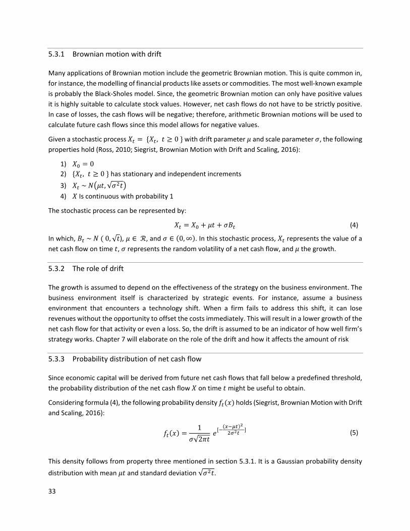
33

5.3.1 Brownian motion with drift

Many applications of Brownian motion include the geometric Brownian motion. This is quite common in, for instance, the modelling of financial products like assets or commodities. The most well-known example is probably the Black-Sholes model. Since, the geometric Brownian motion can only have positive values it is highly suitable to calculate stock values. However, net cash flows do not have to be strictly positive. In case of losses, the cash flows will be negative; therefore, arithmetic Brownian motions will be used to calculate future cash flows since this model allows for negative values.

Given a stochastic process 𝑋𝑋𝑡𝑡 = {𝑋𝑋𝑡𝑡 , 𝐶𝐶 ≥ 0 } with drift parameter 𝜇𝜇 and scale parameter 𝜎𝜎, the following properties hold (Ross, 2010; Siegrist, Brownian Motion with Drift and Scaling, 2016):

1) 𝑋𝑋0 = 0 2) {𝑋𝑋𝑡𝑡 , 𝐶𝐶 ≥ 0 } has stationary and independent increments

3) 𝑋𝑋𝑡𝑡 ~ 𝑁𝑁�𝜇𝜇𝐶𝐶,√𝜎𝜎2𝐶𝐶� 4) 𝑋𝑋 Is continuous with probability 1

The stochastic process can be represented by:

𝑋𝑋𝑡𝑡 = 𝑋𝑋0 + 𝜇𝜇𝐶𝐶 + 𝜎𝜎𝐵𝐵𝑡𝑡 (4)

In which, 𝐵𝐵𝑡𝑡 ~ 𝑁𝑁 ( 0,√𝐶𝐶), 𝜇𝜇 ∈ ℛ, and 𝜎𝜎 ∈ (0,∞). In this stochastic process, 𝑋𝑋𝑡𝑡 represents the value of a net cash flow on time 𝐶𝐶, 𝜎𝜎 represents the random volatility of a net cash flow, and 𝜇𝜇 the growth.

5.3.2 The role of drift

The growth is assumed to depend on the effectiveness of the strategy on the business environment. The business environment itself is characterized by strategic events. For instance, assume a business environment that encounters a technology shift. When a firm fails to address this shift, it can lose revenues without the opportunity to offset the costs immediately. This will result in a lower growth of the net cash flow for that activity or even a loss. So, the drift is assumed to be an indicator of how well firm’s strategy works. Chapter 7 will elaborate on the role of the drift and how it affects the amount of risk

5.3.3 Probability distribution of net cash flow

Since economic capital will be derived from future net cash flows that fall below a predefined threshold, the probability distribution of the net cash flow 𝑋𝑋 on time 𝐶𝐶 might be useful to obtain.

Considering formula (4), the following probability density 𝑜𝑜𝑡𝑡(𝑥𝑥) holds (Siegrist, Brownian Motion with Drift and Scaling, 2016):

𝑜𝑜𝑡𝑡(𝑥𝑥) =

1𝜎𝜎√2𝜋𝜋𝐶𝐶

𝑒𝑒[−(𝑥𝑥−𝜇𝜇𝑡𝑡)2 2𝜎𝜎2𝑡𝑡 ] (5)

This density follows from property three mentioned in section 5.3.1. It is a Gaussian probability density

distribution with mean 𝜇𝜇𝐶𝐶 and standard deviation √𝜎𝜎2𝐶𝐶.

34

5.3.4 Definition

Economic capital for strategic risk, as defined in section 5.2, is a risk measure of earnings falling below a threshold. This threshold is argued to be a firms cost of equity.

Figure 10 illustrates this idea. First, as can be seen in Figure 10, future net cash flows 𝑋𝑋 on time 𝐶𝐶 can take different future paths. In this example, three possible future cash flows are drawn by using the stochastic process from section 5.3. Second, the red dashed line represents the absolute value of the cost of equity. When a net cash flow falls below the red dashed cost of equity line, it is assumed to be in the dangerous zone. It might be worthwhile to note that the red dashed line is just an increasing function served as an example. It is not claimed that the profitability limit have to be a linear increasing line, section 6.3 will elaborate on that.

Figure 10 Examples of possible future net cash flows

When considering the example paths in Figure 10 it could be argued that economic capital in this case should be the amount of capital needed to raise the net income above the red dashed line in any case. Since future earnings are considered, every realization can have a different size of economic capital. This can also be seen in Figure 10, there is one realization that does not come below the red line, and two that do come below the red line. However, those that come below the red line need different amounts of capital to raise the net cash flow above the acceptable limit. In other words, the amount of economic capital needed will be stochastic, since the amount will differ in each possible future scenario. In some cases, zero capital is needed while more in other cases. Therefore, a risk measure is needed to express an acceptable level of economic capital with a single value. Section 3.3, already stated the most common risk measures. Section 5.3.5 will use this theory to define a risk measure for strategic risk.

5.3.5 Risk measure

The objective now is to define a suitable risk measure for the economic capital. Section 5.3.5 in the literature review discusses properties and different types of risk measures defined by the Basel Committee on Banking Supervision (2009). Risk measures that are suitable to use are: value-at-risk,

35

expected shortfall, or spectral risk measures. Since value-at-risk and expected shortfall are the most well-known risk measures in practice and easy to interpret (Basel Committee on Banking Supervision, 2009), the focus will be on those two measures.

As stated in section 5.3.5 the value-at-risk can be defined as the 𝛼𝛼-quantile upper limit of the loss distribution in which alpha is typically a value close to 1. The loss distribution can be obtained by simulation, which will be shown in next chapter. Equation (6), shows the formula for economic capital for one run.

𝐸𝐸𝐶𝐶𝑛𝑛 = �𝑚𝑚𝑎𝑎𝑥𝑥(𝑙𝑙𝑒𝑒𝑚𝑚𝑒𝑒𝐶𝐶 − 𝑥𝑥𝑡𝑡,𝑛𝑛; 0)

𝑡𝑡∈𝑇𝑇

(6)

This can be described as the summation during a specific horizon of all the differences between the profitability limit and the net income. When the net income falls below the limit, the difference equals the gap between the net income and the limit and when it is above that limit, the difference equals zero. It should be noted that the time space is considered to be discreet. This is a legitimate consideration since financial statements will be released in discreet time intervals, such as yearly or quarterly. Therefore, a summation instead of an integral is used in equation (6).

When generating multiple runs, the values of 𝐸𝐸𝐶𝐶 can be used to form a distribution function of economic capital, 𝑜𝑜(𝐸𝐸𝐶𝐶). This distribution function can then be used to find the value at risk by using formula (7) (Righi & Ceretta, 2015; Guégan & Hassini, 2015)

𝑉𝑉𝑎𝑎𝑅𝑅𝛼𝛼(𝐸𝐸𝐶𝐶) = sup{𝑥𝑥|𝐹𝐹(𝐸𝐸𝐶𝐶 < 𝑥𝑥) ≤ 𝛼𝛼}

(7)

Formula (7) gives the value of EC for which holds that the probability of EC being larger than this value equals 1 − 𝛼𝛼. Since 𝛼𝛼 is chosen close to one, for instance, 0.9995; the probability that the EC will be higher than the value at risk is extremely small.

Next to the value-at-risk, the expected shortfall is considered as a measure of risk. As defined in section 5.3.5, the expected shortfall is the average of the tail values beyond the value of risk. In this case, it is the average of the net income values lower than the value-at-risk. Equation 8 shows the equation for the expected shortfall (Righi & Ceretta, 2015).

𝐸𝐸𝑆𝑆𝛼𝛼(𝐸𝐸𝐶𝐶) = 𝐸𝐸[𝐸𝐸𝐶𝐶|𝐸𝐸𝐶𝐶 > 𝑉𝑉𝑎𝑎𝑅𝑅𝛼𝛼(𝐸𝐸𝐶𝐶) =1𝛼𝛼� 𝑉𝑉𝑎𝑎𝑅𝑅𝑠𝑠(𝐸𝐸𝐶𝐶)𝑑𝑑𝐶𝐶1

𝛼𝛼 (8)

As can be seen in formula 8, the expected shortfall is the expectation of all the values higher than the value at risk.

36

Chapter 6: Simulation example

This chapter provides a simulation example of the models discussed in Chapter 5. The objective is to go over the simulation systematically in order to use it as a blue print for other practical implementations. First, section 3.1 elaborates on the data used to calibrate the model. Second, the simulation will be explained. Followed by the result section and sensitivity analysis in which the growth and the cost of equity will be varied.

6.1 Data

The ABN AMRO quarterly reports from 2012 to 2015 were used to obtain the required data (ABN AMRO, 2016). Since these reports are publicly available, confidentiality issues were avoided. The data can be found in Table 13 in Appendix E. As can be seen in Table 13, for each quarter the underlying net profit, equity amount, the return on equity, loan impairments are provided. This data serves as input for the simulations.

The first issue that must be addressed regarding the data are the loan impairments. As discussed in Chapter 5, economic capital for strategic risk is formulated as net profit falling below the profitability limit, in this case the cost of equity. However, the use of net income can have some downsides since it is an accounting value and not a cash flow. More concrete, the goal is to have a figure that reflects the strategy of a business, using net income seems to make sense since this reflect the profitability of a company; however, this should be the net income before any abnormal costs or revenues. For instance, when a company is fined or has to pay legal claims this will affect the profitability of the company; nonetheless, these costs do not have anything to do with the strategic risk as defined in chapter 4. Therefore, it can be argued that the data should be free from abnormal costs or returns. Whether the data from Table 13 is polluted by these abnormal cost or revenues is hard to argue since these are obtained from an annual report on which only consolidated levels of data are provided; for instance, you cannot easily see whether claims are paid unless it is stated in the textual explanations or in secondary sources like newspapers. Since it hard to filter this data with the information we have, this issue of pollution will not be addressed in this example except for one item on the profit and loss statement that is impairment charges on loans and other receivables. Impairments on loans are charges to cover possible loan losses. Although these charges are not related to strategic risk, they significantly affect the result of a bank’s annual statement. This can also be seen in Figure 11, which shows the net underlying profit and the impairments added to the net underlying profit. It can immediately conducted that the blue line is less volatile and contains less outliers than the net profit line. Furthermore, the predicted lines for each time series, which were obtained by simple linear regression, show that the trend of net profit seems to disappear when impairments are added to the series. It can be stated that the positive trend of the net profit is caused by a decrease in impairments over time. This might be due to better processes or stricter rules when providing loans or due to a better economy with a decrease in defaulting obligors. Above all, the trend of the underlying profit seems not to be caused by a better strategy. Furthermore, it could be argued that

37

loan impairments are captured in the regulatory capital for credit risk, include them in the analysis for strategic risk will definitively lead to double counting of risk.

Figure 11 Net Profit v.s. Impairment Charges ABN 2012-2015

Concluding, the data should be free from any expenses or revenues that have no correlation with strategic risk as defined in section 4.2, such as, impairments on loans or operational losses like claims or fines. In other words, net profit before unusual expenses are considered in the assessment of strategic risk. Throughout the rest of this thesis, the term net income will reflect the net profit plus impairments. The data mentioned in Table 13 will be used for model calibration. In particular, the drift and volatility of the Brownian motion must be extracted and the cost of equity must be derived. The drift and volatility will be part of section 6.1.1 and the cost of equity will be dealt with in section 6.1.2.

-100

0

100

200

300

400

500

600

700

800

900

Q1 Q2 Q3 Q4 Q1 Q2 Q3 Q4 Q1 Q2 Q3 Q4 Q1 Q2 Q3 Q4

2012 2012 2012 2012 2013 2013 2013 2013 2014 2014 2014 2014 2015 2015 2015 2015

Net Profit v.s. Net Profit + Impairment Charges

Net Profit + Impairment Net Profit Predicted Net Profit Predicted Net profit + Impairment

38

6.1.1 Parameters for the Brownian motion

The first objective is to estimate the drift and volatility of the Brownian motion stated in equation (4). In order to do that maximum likelihood estimation will be used. Maximum likelihood is a common way to estimate the parameters of time series models (Montgomery & Kulahci, 2008). The maximum likelihood method provides a point estimation of the parameters from an underlying distribution of observations from a random experiment. In other words, an observable random variable 𝑋𝑋 has a density function 𝑜𝑜(. ) with unknown distribution parameter 𝜃𝜃. The maximum likelihood method tries to find a value for 𝜃𝜃 in which the underlying distribution fits the observed values the best.

An assumption for the maximum likelihood method is that all observations have the same density

function. However, when considering formula (5), which was: 𝑜𝑜𝑡𝑡(𝑥𝑥) = 1𝜎𝜎√2𝜋𝜋𝑡𝑡

𝑒𝑒[−(𝑥𝑥−𝜇𝜇𝜇𝜇)2 2𝜎𝜎2𝜇𝜇

], it becomes clear

that this distribution is different for every realization since it depends on the value of 𝐶𝐶. So, every observation 𝑥𝑥𝑡𝑡 is drawn from a different distribution and there is only one observation per time unit. In order to estimate the parameters of the Brownian motion, a joint probability 𝑜𝑜𝑡𝑡1,𝑡𝑡2…,𝑡𝑡𝑛𝑛(𝑥𝑥1, 𝑥𝑥2, … 𝑥𝑥𝑛𝑛) is needed. Fortunately the characteristics of Brownian motions allow to form a joint probability that can be used to estimate the parameters 𝜇𝜇 and 𝜎𝜎.

The joint probability distribution of a Brownian motion with drift is defined as (Siegrist, Maximum Likelihood, 2016):

𝑜𝑜𝑡𝑡1,𝑡𝑡2…,𝑡𝑡𝑛𝑛(𝑥𝑥1, 𝑥𝑥2, … 𝑥𝑥𝑛𝑛) = 𝑜𝑜𝑡𝑡1(𝑥𝑥1) ∗ 𝑜𝑜𝑡𝑡2−𝑡𝑡1(𝑥𝑥2 − 𝑥𝑥1) ∗ … ∗ 𝑜𝑜𝑡𝑡𝑛𝑛−𝑡𝑡𝑛𝑛−1(𝑥𝑥𝑛𝑛 − 𝑥𝑥𝑛𝑛−1) (9)

The joint probability in equation (9) can be proved by using the properties stated in section 5.3.1, which are: stationary and independent increments. Independent means that the increments, 𝑋𝑋𝑡𝑡 − 𝑋𝑋𝑠𝑠 and 𝑋𝑋𝑡𝑡+1 − 𝑋𝑋𝑠𝑠+1 are independent. Stationarity implies that the distribution of 𝑋𝑋𝑡𝑡 − 𝑋𝑋𝑠𝑠 equals the distribution of 𝑋𝑋𝑡𝑡−𝑠𝑠 which is again a Brownian motion with parameters 𝜇𝜇(𝐶𝐶 − 𝐶𝐶) and 𝜎𝜎√𝐶𝐶 − 𝐶𝐶.

When a new time series 𝑒𝑒𝑡𝑡 is created, in which 𝑒𝑒𝑡𝑡 = 𝑥𝑥𝑡𝑡 − 𝑥𝑥𝑡𝑡−1 and 𝑥𝑥𝑡𝑡 is assumed to be an observation of a Brownian stochastic process, 𝑒𝑒𝑡𝑡 is also an observation of the same Brownian stochastic process. Since we use quarterly data the time steps can be valued as: 𝐶𝐶1 = 1, 𝐶𝐶2 = 2 … 𝐶𝐶𝑛𝑛 = 𝑟𝑟. So, the time difference between two subsequent time points equals one. Meaning that the parameters of the stochastic process 𝑌𝑌 equals 𝜇𝜇 and 𝜎𝜎.

Simplifying equation (9) into:

𝑜𝑜(𝑒𝑒1,𝑒𝑒2, … , 𝑒𝑒𝑛𝑛) = 𝑜𝑜(𝑒𝑒1) ∗ 𝑜𝑜(𝑒𝑒) ∗ … ∗ 𝑜𝑜(𝑒𝑒𝑛𝑛) (10)

With,

𝑜𝑜(𝑒𝑒𝑡𝑡) = 1𝜎𝜎√2𝜋𝜋

𝑒𝑒[−(𝑦𝑦𝜇𝜇−𝜇𝜇)2 2𝜎𝜎2

]

Which is a normal distribution. In other words, every observation 𝑒𝑒𝑡𝑡 is a draw from a normal distribution with parameter 𝜇𝜇 and 𝜎𝜎. Which equals the parameter 𝜇𝜇 and 𝜎𝜎 in equation (4), because of the stationary independent increments. Since all observations 𝑒𝑒𝑡𝑡 are now independent and identical distributed, maximum likelihood can be applied. Because 𝑜𝑜(𝑒𝑒𝑡𝑡) is a normal distribution, the maximum likelihood

39

estimation of 𝜇𝜇 and 𝜎𝜎 equals the first and second moment of the normal distribution (Montgomery & Runger, 2002). Resulting in the following estimates:

�̂�𝜇 = 𝑒𝑒� (11)

𝜎𝜎2� =1𝑟𝑟� (𝑒𝑒𝑖𝑖 − �̂�𝜇)2

𝑛𝑛

𝑡𝑡=1 (12)

Concluding, the following steps must be performed on the data to obtain the parameter estimates of the Brownian motion described in equation (4):

1. Create a new time series 𝑒𝑒𝑡𝑡 = 𝑥𝑥𝑡𝑡 − 𝑥𝑥𝑡𝑡−1, with 𝐶𝐶 = {1, . . ,𝑟𝑟}

2. Calculate 𝑒𝑒� = 1𝑛𝑛∑ 𝑒𝑒𝑡𝑡𝑛𝑛𝑡𝑡=1 = �̂�𝜇

3. Calculate 𝜎𝜎2� = 1𝑛𝑛∑ (𝑒𝑒𝑖𝑖 − �̂�𝜇)2𝑛𝑛𝑡𝑡=1

The application of the three steps to obtain the estimations can be found in Appendix F.

Since it is assumed that the variable 𝑌𝑌 has a normal density function, the observations 𝑒𝑒𝑡𝑡 in Appendix F should be tested on normality. This is done in R with a Shapiro-Wilks test of normality, which resulted in a P value of 0.1839. The null-hypotheses that the underlying distribution has a normal distribution can be accepted.

6.1.2 Estimating the Cost of Equity

Next to the values of 𝜇𝜇 and 𝜎𝜎, the cost of equity has to be estimated. In order to obtain the profitability limit. As discussed in 5.2 the cost of equity equals the required rate of return, which can be extracted from the CAPM formula. With the rate or return, an absolute value of the cost of equity can be obtained by multiplying the rate of return with the average amount of equity, as also stated in formula (3). Since we are dealing with quarterly data, the average equity is calculated as the total equity in a specific quarter divided by four. It might be worthwhile to note that the net income is increased with the loan impairments, resulting in a higher figure then only considering net income without impairments. This implicates that the economic capital will be lower since the probability of falling below the cost of equity will be reduced, which is a desired effect because impairments (and other unusual credit or operational costs) should not have any effect on the economic capital for strategic risk.

The first objective is to determine the required rate of return. By using the company beta of ABN AMRO, the expected market return and the risk free rate. However, ABN AMRO recently had their IPO that makes it hard to estimate the beta of the company. To deal with this, a range of betas will be considered varying between 0,8 and 1,5. This range is based on the beta’s of comparable banks. Section 6.3 will deal with the varying beta and the effect it has on the economic capital. Next to data issues, it is interesting to look to a changing level of the cost of equity since the beta is based on historical data, meaning that it always lags behind the ‘real’ beta. For now, it is assumed that ABN AMRO has a beta of 1.15, which equals the beta of ING bank.

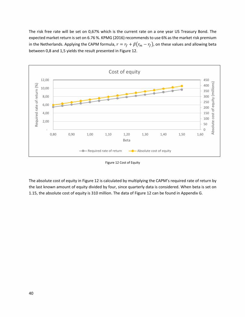
40

The risk free rate will be set on 0,67% which is the current rate on a one year US Treasury Bond. The expected market return is set on 6.76 %. KPMG (2016) recommends to use 6% as the market risk premium in the Netherlands. Applying the CAPM formula, 𝑟𝑟 = 𝑟𝑟𝑓𝑓 + 𝛽𝛽�𝑟𝑟𝑚𝑚 − 𝑟𝑟𝑓𝑓�, on these values and allowing beta between 0,8 and 1,5 yields the result presented in Figure 12.

Figure 12 Cost of Equity

The absolute cost of equity in Figure 12 is calculated by multiplying the CAPM’s required rate of return by the last known amount of equity divided by four, since quarterly data is considered. When beta is set on 1.15, the absolute cost of equity is 310 million. The data of Figure 12 can be found in Appendix G.

050100150200250300350400450

-

2,00

4,00

6,00

8,00

10,00

12,00

0,80 0,90 1,00 1,10 1,20 1,30 1,40 1,50 1,60 Abso

lute

cos

t of e

quity

(mill

ions

)

Requ

ired

rate

of r

etur

n (%

)

Beta

Cost of equity

Required rate of return Absolute cost of equity

41

6.2 Simulation

6.2.1 Simulation procedure

This section elaborates on the simulation. First, the content of the simulation will be briefly discussed by commenting on the code in Appendix H page 71. Second, this section will validate that the outcome of the simulation equals the theoretical results that can be obtained by using the probability distributions of the Brownian motion. The first simulation will assume all parameters to be constant.

As discussed in section 5.3.5, the objective is to find the distribution of the economic capital 𝑜𝑜(𝐸𝐸𝐶𝐶). The economic capital per run was given by:

𝐸𝐸𝐶𝐶𝑛𝑛 = �𝑚𝑚𝑎𝑎𝑥𝑥(𝑙𝑙𝑒𝑒𝑚𝑚𝑒𝑒𝐶𝐶 − 𝑥𝑥𝑡𝑡,𝑛𝑛; 0)𝑡𝑡∈𝑇𝑇

The simulation, which can be found in Appendix H, roughly entails the following steps.

• First, a matrix is created containing Brownian paths {𝑥𝑥0, . . , 𝑥𝑥𝑇𝑇} on the rows; in which, 𝑥𝑥0 is assumed to be the last known value available, and {𝑥𝑥1, … , 𝑥𝑥𝑇𝑇} are the results of the Brownian motion. Furthermore, each column in the matrix represents one run.

• Second, every value in this matrix is checked to be under or above the cost of equity. If it falls above the cost of equity, the value in the matrix is neglected. If the value falls below the cost of equity, then this value is subtracted from the cost of equity to obtain the difference between the realization and the cost of equity. The result of this subtraction is added up per run for every 𝐶𝐶. The table below shows a schematic overview of this procedure. Since economic capital for strategic risk is evaluated over a certain strategy horizon, all the rows per column are added up to obtain a vector with the length that equals the number of runs and each entry representing the economic capital needed for the time horizon of that run.

Run 1 Run 2 …. …. …. Run n t=1 0 150 …. …. …. 80 …. …. …. …. …. …. …. t=T 200 0 …. …. …. 20 �

𝑡𝑡∈𝑇𝑇

� 𝑡𝑡∈𝑇𝑇

…. …. …. � 𝑡𝑡∈𝑇𝑇

• Last, this vector is sorted in ascending order to easily obtain the value at risk. This can be done by multiplying the length of the vector with alpha. For instance, when the length of the vector equals 10.000 and alpha is 0.95, the value at risk is the 9.500th element in the vector.

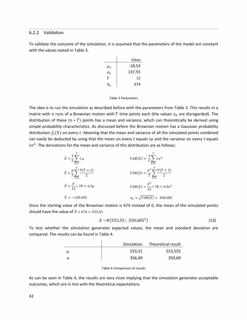
42

6.2.2 Validation

To validate the outcome of the simulation, it is assumed that the parameters of the model are constant with the values stated in Table 3.

Value

𝜇𝜇𝑋𝑋 -18,53 𝜎𝜎𝑋𝑋 137,55 𝑇𝑇 12 𝑋𝑋0 674

Table 3 Parameters

The idea is to run the simulation as described before with the parameters from Table 3. This results in a matrix with 𝑟𝑟 runs of a Brownian motion with 𝑇𝑇 time points each (the values 𝑥𝑥0 are disregarded). The distribution of these (𝑟𝑟 ∗ 𝑇𝑇) points has a mean and variance, which can theoretically be derived using simple probability characteristics. As discussed before the Brownian motion has a Gaussian probability distribution 𝑜𝑜𝑡𝑡(𝑋𝑋) on every 𝐶𝐶. Meaning that the mean and variance of all the simulated points combined can easily be deducted by using that the mean on every 𝐶𝐶 equals 𝐶𝐶𝜇𝜇 and the variance on every 𝐶𝐶 equals 𝐶𝐶𝜎𝜎2. The derivations for the mean and variance of this distribution are as follows:

𝑋𝑋� =1𝑇𝑇�𝐶𝐶

𝑇𝑇

𝑡𝑡=1

𝜇𝜇 𝑉𝑉𝑉𝑉𝑅𝑅(𝑋𝑋) = 1𝑇𝑇�𝐶𝐶

𝑇𝑇

𝑡𝑡=1

𝜎𝜎2

𝑋𝑋� =𝜇𝜇𝑇𝑇�

𝑇𝑇(𝑇𝑇 + 1)2

𝑇𝑇

𝑡𝑡=1

𝑉𝑉𝑉𝑉𝑅𝑅(𝑋𝑋) =𝜎𝜎2

𝑇𝑇 �𝑇𝑇(𝑇𝑇 + 1)

2 𝑇𝑇

𝑡𝑡=1

𝑋𝑋� =𝜇𝜇

12 ∗ 78 = 6.5𝜇𝜇 𝑉𝑉𝑉𝑉𝑅𝑅(𝑋𝑋) =𝜎𝜎2

12 ∗ 78 = 6.5𝜎𝜎2

𝑋𝑋� = −120.445 𝜎𝜎𝑋𝑋 = �𝑉𝑉𝑉𝑉𝑅𝑅(𝑋𝑋) = 350.685

Since the starting value of the Brownian motion is 674 instead of 0, the mean of the simulated points should have the value of 𝑋𝑋� + 674 = 553,55.

𝑋𝑋 ~𝑁𝑁(553,55 ; 350.6852) (13)

To test whether the simulation generates expected values, the mean and standard deviation are compared. The results can be found in Table 4.

Simulation Theoretical result

𝜇𝜇 553,31 553,555 𝜎𝜎 356,49 350,69

Table 4 Comparison of results

As can be seen in Table 4, the results are very close implying that the simulation generates acceptable outcomes, which are in line with the theoretical expectations.

43

6.3 Results

To start off, the simulation described in section 6.2 is performed with the constant parameters stated in Table 5.

Parameter value 𝜇𝜇 -18,53 𝜎𝜎 137,55 𝑥𝑥0 674 𝐿𝐿𝑒𝑒𝑚𝑚𝑒𝑒𝐶𝐶 310 𝑇𝑇 12 𝛼𝛼 0,9995 Table 5 Parameter values

The code of this simulation can be found on page 71 in Appendix H. The first result that must be discussed is the density of the net income. Figure 13 shows the histogram of the net income values that were generated in the simulation with 1 million runs. These values include all realizations of quarterly net income on all values of 𝐶𝐶. In other words, it is the density of a value of net income on a random point in time.

Next to the net income, the distribution of economic capital is obtained. Per run, the economic capital amount is defined as ∑ 𝑚𝑚𝑒𝑒𝑟𝑟(𝑙𝑙𝑒𝑒𝑚𝑚𝑒𝑒𝐶𝐶 − 𝑥𝑥𝑡𝑡; 0)𝑡𝑡∈𝑡𝑡 for 𝐶𝐶 = 1, … ,𝑇𝑇. With the parameters from Table 5, this results in the capital needed per run to cover for strategic risk over a three years horizon. The density of economic capital is given in Figure 14. The 99.95% upper limit of this distribution is the value at risk (VaR) as defined in section 5.3.5 and indicated with the red line in Figure 14.

Figure 13 Density of net income

44

As can be seen, the VaR for a three years horizon equals 2,882 billion euros, which equals 0,961 billion euros per year. In 2014, ABN AMRO reported 1,143 billion euros economic capital for strategic risk. Which is slightly more than the result in Figure 14.

In the previous simulations, the cost of equity is assumed to be a constant value. However, this might not be a reasonable assumption. Although a constant threshold might be a defendable assumption given the short time range of the simulation, it is likely that the amount of equity will change over time. The equity amount in banking firms is already increasing due to legislation requirements. Furthermore, many banks have internal goals to increase the equity amount to have a more sustainable capital base. To test the effect of a changing cost of equity over time, the simulation will be adapted and allow the profitability limit to increase over time. Before the simulation can be adapted, it is first tested whether the hypotheses of an increasing equity amount holds for ABN AMRO. To test this, simple linear regression represented in equation (14) is applied to the equity data in Table 13.

𝑒𝑒𝑡𝑡 = 𝛽𝛽0 + 𝑥𝑥𝑡𝑡𝛽𝛽𝑡𝑡 + 𝜖𝜖 (14)

Equation (14) tests whether a trend exists in the data. Variable 𝑒𝑒𝑡𝑡 represents the quarterly equity amount on 𝐶𝐶 = {1,2,3, . . . ,𝑇𝑇} and variable 𝑥𝑥𝑡𝑡 represents the number of the quarter 𝑥𝑥𝑡𝑡 = {1,2, … ,𝑇𝑇}. Furthermore, 𝛽𝛽0 is the intercept of the model and 𝛽𝛽1the coefficient, which equals the increase in equity per quarter. The results of the regression are stated in Table 6.

Coefficient P-value 𝑉𝑉𝑑𝑑𝐴𝐴.𝑅𝑅2

Intercept (𝛽𝛽0) 12697,25 1,00483E-16

COE (𝛽𝛽1) 187,7721 1,13894E-05

Model statistic 0,741 Table 6 Regression output for the equity amount

As can be seen in Table 6, the hypotheses that the equity amount is increasing over time can be accepted. The model has a significant predictability with the adjusted 𝑅𝑅2 equals 0,741. Furthermore, all variables in the model are significant with p-values far below the 0,05 limit.

Figure 14 Density of economic capital

45

The objective is now to include the results in the simulation. Since it is established that the equity amount has a trend. The profitability limit will be changed in a linear function of time. Again 𝛽𝛽 is assumed to be 1,15 as also argued in section 6.1.2. The corresponding required rate of return, which was 7,57%, is multiplied with the last known equity amount of the fourth quarter in 2015, yielding a profitability limit of 310 million. This will be the intercept of the linear function stated in equation (15) and is indicated as 𝑙𝑙𝑒𝑒𝑚𝑚𝑒𝑒𝐶𝐶0. Next to that, the quarterly increase is calculated as the increase in equity, 𝛽𝛽1 in Table 6, multiplied with the required rate of return, which is 3,553 and indicated as 𝛽𝛽1 ∗ 𝑟𝑟 in equation (15).

𝑙𝑙𝑒𝑒𝑚𝑚𝑒𝑒𝐶𝐶𝑡𝑡 = 𝑙𝑙𝑒𝑒𝑚𝑚𝑒𝑒𝐶𝐶0 + 𝐶𝐶 ∗ 𝛽𝛽1 ∗ 𝑟𝑟 (15)

When equation (15) is applied in the simulation with 1 million runs, the value at risk increases to 3022,37. The result of the simulation can be found in Figure 15. Furthermore, the code of this simulation can be found in Appendix H on page 72.

As can be seen in Figure 15, the density of economic capital differs with the density in Figure 14. The highest point has slightly moved to right, which is a logic result since an increase in the profitability limit will lead to higher demands in the future and therefore result in higher values of economic capital. However, the value at risk is not tremendously higher than the value reported in Figure 14. So, the effect of the model improvement has no surprising effects. The results of this section are graphically represented in Figure 16.

Figure 15 Economic capital with increasing COE

46

Concluding, this section resulted in three values of economic capital for strategic risk. First, economic capital was calculated for the case in which all parameters were assumed to be constant. Second, an improvement to the model was made by allowing the absolute cost of equity to increase over time. This resulted in a slightly higher value at risk, which was 1007,45 million with the increasing cost of equity and 960,995 million without. All results were slightly lower than the reported economic capital for strategic risk by ABN AMRO in 2014; however, they do not tremendously deviate from the reported figure by ABN.

6.4 Simulation accuracy

In the above simulation, one million runs are performed to obtain the value at risks in Figure 16. This section will address the accuracy of these values.

To assess the accuracy of one million runs, the simulation was broken down into 100 blocks with each block containing 10.000 runs. For every block, the value at risk was calculated. Figure 17 shows the results of these simulations. Furthermore, the code of this simulation can be found on page 73 in Appendix H.

Figure 17 simulation accuracy

0

200

400

600

800

1000

1200

Annual report Constantparameters

Increasing COE

Economic capital

Figure 16 Economic capital comparison

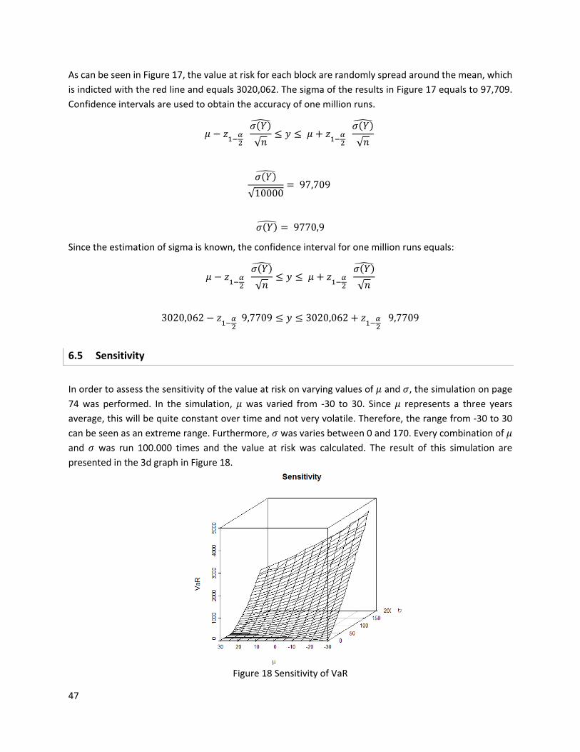
47

As can be seen in Figure 17, the value at risk for each block are randomly spread around the mean, which is indicted with the red line and equals 3020,062. The sigma of the results in Figure 17 equals to 97,709. Confidence intervals are used to obtain the accuracy of one million runs.

𝜇𝜇 − 𝑧𝑧1−𝛼𝛼2 𝜎𝜎(𝑌𝑌)�

√𝑟𝑟≤ 𝑒𝑒 ≤ 𝜇𝜇 + 𝑧𝑧1−𝛼𝛼2

𝜎𝜎(𝑌𝑌)�

√𝑟𝑟

𝜎𝜎(𝑌𝑌)�

√10000= 97,709

𝜎𝜎(𝑌𝑌)� = 9770,9

Since the estimation of sigma is known, the confidence interval for one million runs equals:

𝜇𝜇 − 𝑧𝑧1−𝛼𝛼2 𝜎𝜎(𝑌𝑌)�

√𝑟𝑟≤ 𝑒𝑒 ≤ 𝜇𝜇 + 𝑧𝑧1−𝛼𝛼2

𝜎𝜎(𝑌𝑌)�

√𝑟𝑟

3020,062 − 𝑧𝑧1−𝛼𝛼2

9,7709 ≤ 𝑒𝑒 ≤ 3020,062 + 𝑧𝑧1−𝛼𝛼2 9,7709

6.5 Sensitivity

In order to assess the sensitivity of the value at risk on varying values of 𝜇𝜇 and 𝜎𝜎, the simulation on page 74 was performed. In the simulation, 𝜇𝜇 was varied from -30 to 30. Since 𝜇𝜇 represents a three years average, this will be quite constant over time and not very volatile. Therefore, the range from -30 to 30 can be seen as an extreme range. Furthermore, 𝜎𝜎 was varies between 0 and 170. Every combination of 𝜇𝜇 and 𝜎𝜎 was run 100.000 times and the value at risk was calculated. The result of this simulation are presented in the 3d graph in Figure 18.

Figure 18 Sensitivity of VaR

48

As can be seen in Figure 18, the relation between value at risk, 𝜇𝜇, and 𝜎𝜎 forms a 3d surface. The results seems straightforward, when 𝜇𝜇 is high the value at risk will increase with a lower rate compared to lower values of 𝜇𝜇. The same logic holds for 𝜎𝜎.

An important implication of this sensitivity graph is the relation between 𝜇𝜇 and 𝜎𝜎. It can be argued that an attempt to increase 𝜇𝜇 during a strategic horizon will lead to higher amounts of risk in the nearby future. Therefore, it is important to know how the value at risk will change when the parameter of the models change. To assess the impact of changes in 𝜇𝜇 and 𝜎𝜎 on a more detailed level than presented in Figure 18, the first objective will be to search for the combinations of 𝜇𝜇 and 𝜎𝜎 in which the value at risk remains the same. This will lead to a scenario in which an attempt to increase 𝜇𝜇 will change 𝜎𝜎 and the combination of those two will not lead to a decrease in the value at risk. In other words, it is not viable to invest since it will not pay off in terms of risk.

Previous chapter established that the mean value at risk for the given model parameters equals 3020,062. When this value is plotted as a surface in Figure 18, the intersection with the graph would provide all combination of 𝜇𝜇 and 𝜎𝜎 for which the value at risk is 3020,062. This idea is graphically shown in Figure 19.

Figure 19 Sensitivity of VaR

To find the combinations for which the value at risk remains the same, the simulation started on page 74 looks for the values at risk that are between the confidence interval:

020,062 − 1.96 ∗9770,9�(105)

≤ 𝑒𝑒 ≤ 3020,062 + 1.96 ∗ 9770,9�(105)

49

And returns the corresponding values of 𝜇𝜇 and 𝜎𝜎 on which the graph in Figure 19 intersects the red surface. The resulting combinations are presented in Figure 20.

As can be seen in Figure 20, the combinations of 𝜇𝜇 and 𝜎𝜎 have a linear relation. Which is also indicated in the right graph in which the fitted line is plotted. The fitted line is obtained by simple linear regression from which the statistics can be found in Table 7. It can be conducted from Table 7, that there is a strong linear relation between 𝜇𝜇 and 𝜎𝜎 when the value at risk remains the same.

Coefficient P-value 𝑉𝑉𝑑𝑑𝐴𝐴.𝑅𝑅2 Intercept 166,452 8,37E-10

𝜇𝜇 1,613 1,20E-05 Model 0,9802

Table 7 Regression statistics

The results in Figure 20 and Table 7 can be used to further assess the sensitivity of the value at risk. When the objective is to increase 𝜇𝜇, it might be interesting to know how the value at risk changes. However as discussed before, it can be assumed that 𝜎𝜎 will increase as well. To assess the effect on the value at risk, two scenarios will be discussed. These scenarios are indicated in Figure 21. The fitted line will represent the base scenario in which the value at risk will remain the same, regardless of the values of 𝜇𝜇.

Figure 20 Relation of 𝜇𝜇 and 𝜎𝜎 for which the value at risk remains 3020.062

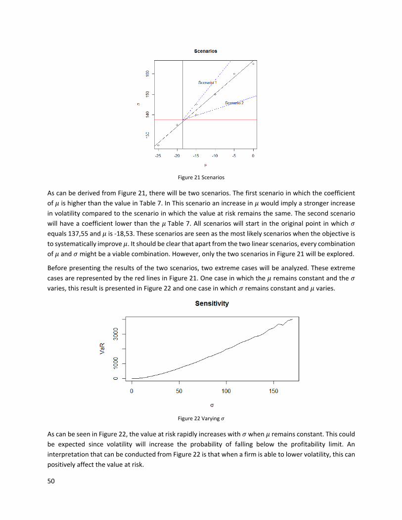
50

Figure 21 Scenarios

As can be derived from Figure 21, there will be two scenarios. The first scenario in which the coefficient of 𝜇𝜇 is higher than the value in Table 7. In This scenario an increase in 𝜇𝜇 would imply a stronger increase in volatility compared to the scenario in which the value at risk remains the same. The second scenario will have a coefficient lower than the 𝜇𝜇 Table 7. All scenarios will start in the original point in which 𝜎𝜎 equals 137,55 and 𝜇𝜇 is -18,53. These scenarios are seen as the most likely scenarios when the objective is to systematically improve 𝜇𝜇. It should be clear that apart from the two linear scenarios, every combination of 𝜇𝜇 and 𝜎𝜎 might be a viable combination. However, only the two scenarios in Figure 21 will be explored.

Before presenting the results of the two scenarios, two extreme cases will be analyzed. These extreme cases are represented by the red lines in Figure 21. One case in which the 𝜇𝜇 remains constant and the 𝜎𝜎 varies, this result is presented in Figure 22 and one case in which 𝜎𝜎 remains constant and 𝜇𝜇 varies.

Figure 22 Varying 𝜎𝜎

As can be seen in Figure 22, the value at risk rapidly increases with 𝜎𝜎 when 𝜇𝜇 remains constant. This could be expected since volatility will increase the probability of falling below the profitability limit. An interpretation that can be conducted from Figure 22 is that when a firm is able to lower volatility, this can positively affect the value at risk.

51

Figure 23 Varying 𝜇𝜇

As can be seen in Figure 23 the value at risk declines rapidly when mu is changed. Meaning that a small effort to increase growth can have a large influence on the value at risk for strategic risk. Although the decline is rapid for lower levels of 𝜇𝜇, it can be conducted from Figure 23 that the decline is less for higher values for 𝜇𝜇. This can easily be explained since economic capital can only have positive values, there will be an asymptotic decay on zero when 𝜇𝜇 increases since the probability of falling below the profitability limit will decrease. The interpretation to strategic risk might be that not every investment to raise the value of 𝜇𝜇 is worthwhile to consider, since it can have a smaller effect on the value at risk than the amount of the investment.

To evaluate the sensitivity on the value at risk of the scenarios described in Figure 21, the script on page 76 in Appendix H was used. The script is roughly the same as used before. In these simulations, however, first two vectors of the same length containing either values for 𝜇𝜇 or 𝜎𝜎 were defined to obtain the linear combination of 𝜇𝜇 and 𝜎𝜎. After that, all combinations where run 10^5 times. For every combinations of 𝜇𝜇 and 𝜎𝜎 a value at risks was obtained. Both scenarios started in the points 𝜎𝜎 = 137,55 and 𝜇𝜇 = -18,53. The coefficient of 𝜇𝜇 in Table 7 equals 3 in the first scenario and 0.5 in the second. These values, which are stated in Table 8, were taken arbitrary. The exact linear combinations of 𝜇𝜇 and 𝜎𝜎 for both scenarios can be found in Appendix I on page 77.

Scenario 1 Scenario 2 𝜎𝜎𝑠𝑠𝑡𝑡𝑠𝑠𝑠𝑠𝑡𝑡 137,55 137,55 𝜇𝜇𝑠𝑠𝑡𝑡𝑠𝑠𝑠𝑠𝑡𝑡 -18,53 -18,53 𝜇𝜇𝑐𝑐𝑐𝑐𝑐𝑐𝑓𝑓 3 0,5

Table 8 Scenario values

The result of the first scenario can be found in Figure 24. The left graph shows the result in a 3d graph and can be interpreted as the path of the linear combinations between 𝜇𝜇 and 𝜎𝜎 on the surface in Figure 19. The right path shows the result in 2d the exact combinations of 𝜇𝜇 and 𝜎𝜎 can be found in Appendix I.

52

As can be seen in Figure 24, the value at risk increases in scenario 1. This could be expected since the sigma increases rapidly compared to the base scenario in which the value at risk remains the same. It should again be noted that 𝜇𝜇 is a long term average, meaning that a change of 𝜇𝜇 from -18,53 to 30 is not likely to occur. Scenario 1 can be interpreted as a strategy scenario in which 𝜇𝜇 can be increased, however, the activities to increase 𝜇𝜇 will lead to a higher risk. It is therefore, important that the risk will decrease again after some period. Otherwise, 𝜇𝜇 has increased but not contributed to lower risk.

The results of the second scenario are stated in Figure 25, again in a 3d and 2d graph. The second scenario, as indicated in Figure 21, also aims to increase 𝜇𝜇; however, the growth of sigma is lower than the base scenario. It might be important to note that 𝜎𝜎 still increases when 𝜇𝜇 increases only with a lower growth rate.

Figure 24 Result scenario 1

Figure 25 Result scenario 2

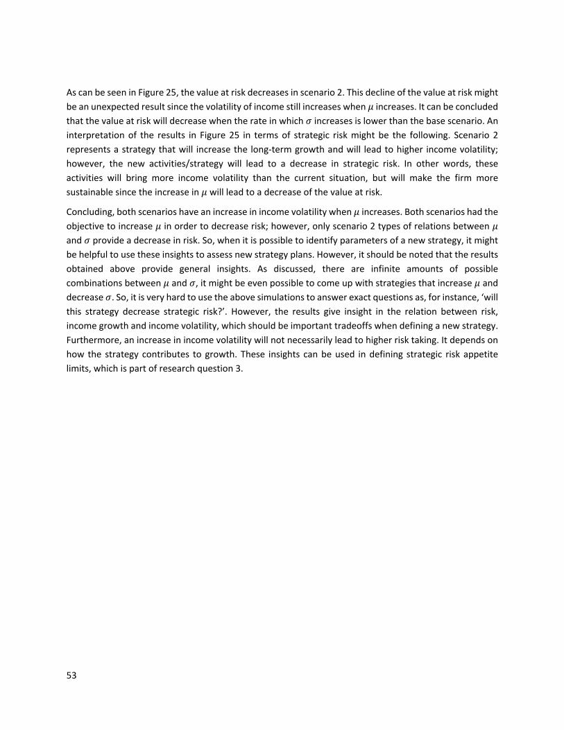
53

As can be seen in Figure 25, the value at risk decreases in scenario 2. This decline of the value at risk might be an unexpected result since the volatility of income still increases when 𝜇𝜇 increases. It can be concluded that the value at risk will decrease when the rate in which 𝜎𝜎 increases is lower than the base scenario. An interpretation of the results in Figure 25 in terms of strategic risk might be the following. Scenario 2 represents a strategy that will increase the long-term growth and will lead to higher income volatility; however, the new activities/strategy will lead to a decrease in strategic risk. In other words, these activities will bring more income volatility than the current situation, but will make the firm more sustainable since the increase in 𝜇𝜇 will lead to a decrease of the value at risk.

Concluding, both scenarios have an increase in income volatility when 𝜇𝜇 increases. Both scenarios had the objective to increase 𝜇𝜇 in order to decrease risk; however, only scenario 2 types of relations between 𝜇𝜇 and 𝜎𝜎 provide a decrease in risk. So, when it is possible to identify parameters of a new strategy, it might be helpful to use these insights to assess new strategy plans. However, it should be noted that the results obtained above provide general insights. As discussed, there are infinite amounts of possible combinations between 𝜇𝜇 and 𝜎𝜎, it might be even possible to come up with strategies that increase 𝜇𝜇 and decrease 𝜎𝜎. So, it is very hard to use the above simulations to answer exact questions as, for instance, ‘will this strategy decrease strategic risk?’. However, the results give insight in the relation between risk, income growth and income volatility, which should be important tradeoffs when defining a new strategy. Furthermore, an increase in income volatility will not necessarily lead to higher risk taking. It depends on how the strategy contributes to growth. These insights can be used in defining strategic risk appetite limits, which is part of research question 3.

54

Chapter 7: Conclusion

This chapter will conclude the insights of these master thesis. Section 7.1 will provide a recap of the research questions and answers that were obtained. Furthermore, it will discuss the relevance and contribution to literature and its shortcomings. Section 7.2 will address the practical insights that were obtained. Section 7.3 will discuss some recommendation for future research. Last, section 7.4 will address the rigor and relevance of this thesis.

7.1 Research conclusion

The first sub question, ‘What is a quantifiable definition of strategic risk for financial institutions?’, was answered in chapter 4. After conducting extensive research to definitions in literature, regulations and in annual statements a definitions was constructed and validated with interviews among experts in the field. Definitions of the BCBS (2009), Slywotzky and Drzik (2005), Schroeck (2002), and Doff (2009) served as an important input for the definitions. Specially Slywotzky and Drzik (2005), who provided clear external trends and events of strategic risk that were: Industry margin squeeze, technology shift, brand erosion, one-of-a-kind competitor, customer priority shift, new-project failure, and market stagnation. Furthermore, an important contribution to literature is the position regarding income volatility. In literature, strategic risk was seen as loss due to income volatility; whereas some annual statements referred to strategic risk with deviation from expected income. After the interviews, we established the position that deviation from expected income is more suitable than only consider loss.

The second sub question, ‘What is a suitable model to calculate economic capital for strategic risk?’, was answered in chapter 5. We proposed to model net income as a stochastic process and to see net income as a performance measure of strategy, since a good strategy will lead to higher incomes. Following the model of Böcker (2008), an arithmetic Brownian motion with drift and volatility was introduced as a suitable stochastic process for future net income values. Furthermore, CAPM was used to estimate the profitability limit of net income by calculating the absolute cost of equity. All realization below the cost of equity imply an underperformance in terms of return. Last, economic capital and risk measures (value at risk and expected shortfall) were defined using the theory and best practices on risk measures from the BCBS (2009). The model was applied to data from ABN AMRO, to check whether the results make sense. Since ABN AMRO reported economic capital on strategic risk in the annual reports, we were able to compare the model results with the reported amount. It was concluded that the result were very close and that the model obtained a slightly lower amount of economic capital. Using ABN as a case study, was somewhat challenging since ABN just recently had an IPO making it hard to estimate the company’s beta. Furthermore, only aggregated data from the publicly available reports were used making it difficult to identify outliers or unusual expenses that should be corrected for in the income figures. However, the result was surprisingly close to the reported amount making it arguable that the model generates useful output.

55

The last sub question, ‘Can these calculations help to set risk appetite limits in order to monitor strategic risk?’, can partially be answered. The sensitivity results provide some insights how risk changes when parameters are being adjusted. The insights of these sensitivity analyses can be used by managers; however, the results do not provide strict limits to monitor strategic risk on an ongoing basis. Furthermore, it depends heavily on the data and the model assumptions. Therefore, hard objective monitoring cannot yet be done based on these simulations. However, more case studies might provide insight in the usefulness of this model when defining risk appetite limits.

Concluding, the model seems a surprisingly simple but effective tool to use in the assessment of strategic risk. So, to the best of our knowledge and based on the results of this thesis, the main question: ‘Can economic capital for strategic risk be calculated?’, can positively be confirmed. Furthermore, the model provided useful practical insights that will be referred to in next section.

7.2 Practical insights

The first practical insight can be obtained from the definition. It is clearly indicated throughout the thesis, that banks use different definitions in annual statements. In addition to that, regulation does not provide clarity of definitions either. The definition obtained in this report is extensive and useful to practitioners. It is our opinion that the definition gives many details regarding, for instance, the external trends and events, and the activities that are affected by it.

Next to the definition, the model has proven to generate an acceptable outcome. In the example of ABN AMRO the result was surprisingly close to the reported amount making it arguable that the model can be used for other, may be smaller banks. It is at least an effective and simple model to discus with the supervisors when addressing strategic risk under the pillar 2 regulations. It was concluded from the interviews that the Dutch supervisor can arbitrary assign amounts of capital to strategic risk without support of models. The model in this thesis could be help in these discussions for both supervisors as for banks.

Furthermore, the sensitivity analysis of the model generated some interesting results. Although the analysis is somewhat abstract, it showed how some strategies, even when they increase growth, will not help to decrease the amount of risk. These kinds of analysis could be used to set up frameworks for better decision making or to identify good or bad strategies. Even when it is impossible to get exact outcomes of these analyses, they can be very useful in providing qualitative insights to managers.

7.3 Future research

Future research regarding strategic risk should first focus on converging contents. One important observation from the thesis is that the content of strategic risk, such as definitions or models, highly vary. A future objective would be to agree upon and standardize this content. It is our opinion that legislation can play a major role in this objective

56

Furthermore, much attention should be given to the practical aspects of strategic risk. It is important that results from future research contribute to relevant insights. It should help managers in creating risk frameworks, so future research should contribute to that. There is much literature regarding strategy; however, strategic risk frameworks based on quantitative models are rare. This thesis can give a starting point in this direction. Next to that, it can be interesting to apply this model on a business unit level to identify weak business parts or to prioritize strategy activities to those business units that need it the most. Last, this thesis used net income plus impairments as a measure of strategy performance. This measure might be majorly improved by research into relevant costs and incomes. However, more detailed knowledge and practical experience into accounting for banks is required for this.

7.4 Rigor and relevance

We want to address the rigor and relevance debate in order to clarify the position of the thesis. In managements science there is an ongoing discussion between rigor and practical usefulness of research (Shrivastava, 1987). This discussion also applies to this research and should therefore shortly be addressed, since this research uses formal models to design a solution for the research problem. It is important to note that the modelling in this thesis uses idealizations in terms of which aspects are modelled and which not, mathematical assumptions, and generalizations. Therefore, cautiousness should be in place when applying these models in practice, since the models cannot be seen as hard science; such as, law of gravity in physics. The aim of this thesis was to both address rigor on relevance. Since the thesis was commissioned by KPMG, relevance is important to be able to use the results in practice. However, rigor is an important aspect as well since the master thesis should contribute to literature and to standards in operations management. Our opinion is that the gap between rigor and relevance is minimized as much as possible. We argue that the thesis is sufficiently rigor to the type of research conducted. The research can be framed as axiomatic research which Bertrand and Fransoo (2002) define as: the research in which solutions give insight to the problem as defined within the idealized model. The thesis uses a sufficient amount of formal models, methods and techniques within mathematics and statistics; furthermore, the thesis manipulates parameters to obtain useful insights in the sensitivity section and it provides a solution to the research problem. The thesis can also considered relevant according to criteria mentioned by Bertrand and Fransoo (2002), since it can assist managers in calculating the value at risk for strategic risk. This could help small firms and large firms in the discussion with the supervisor. Furthermore, strategic risk increasingly gets attention in regulation; therefore, the results in this thesis might be useful for both regulators as practitioners.

57

Chapter 8: References

ABN AMRO. (2016, March 4). Financiele resultaten. Retrieved from ABN AMRO: https://www.abnamro.com/nl/images/Documents/050_Investor_Relations/2015/ABN_AMRO_Q4_2015_factsheet.xlsx

Acerbi. (2002). Spectral measures of risk: A coherent representation of subjective risk aversion. Journal of Banking & Finance, 1505-1518.

al., M. e. (2008). Introduction to Time Series Analysis and Forecasting. New Jersey: John Wiley & Sons.

Bank of International Settlements. (2013). Charter. Basel: Bank of International Settlements.

Bank of international Settlements. (2014, 10 17). About BIS. Retrieved from The Bank of International Settlements: https://www.bis.org/about/index.htm

Basel Committee on Banking Supervision. (2006). International Convergence of Capital Measurement and Capital Standards. Basel: Bank for International Settlements.

Basel Committee on Banking Supervision. (2009). Range of practices and issues in economic capital frameworks. Basel: Bank of International Settlements.

Basel Committee on Banking Supervision. (2011). Principles for the Sound Management of Operational Risk. Basel: BIS.

Basel Committee on Banking Supervision. (2015). Guidelines for identifying and dealing with weak banks. Bank For International Settlements.

Berger, A., Hering, R., & Giorgio, P. (1995). The role of capital in financial firms. Jornal of banking & finance, 393-430.

Bertrand, J., & Fransoo, J. (2002). Operations management research methodologies using quantitative modeling. International Journal of Operations & Production Management, 241-264.

Böcker, K. (2008). Modelling and Measuring Business Risk. In A. Resti, Pillar II in the New Basel Accord–The Challenge of Economic Capital (pp. 179-200). New York: Risk Books.

Brockwell, P. (2009). Handbook of Financial Time Series. In T. Andersen et al., An Overview of Asset-Price Models (pp. 403-419). Berlin: Springer.

Damodaran, A. (2016, March 7). Annual Returns on Stock, T.Bonds and T.Bills: 1928 - Current. Retrieved from NYU Stern school of business: http://pages.stern.nyu.edu/~adamodar/New_Home_Page/datafile/histretSP.html

De Nederlandsche Bank. (2007). Supervisor’s Manual to the Supervisory Review & Evaluation Process (SREP). DNB. Retrieved from http://www.toezicht.dnb.nl/binaries/50-212123.pdf

Deutsche Bank. (2016). Annual report 2015. Retrieved from https://annualreport.deutsche-bank.com/2015/ar/servicepages/downloads/files/dbfy2015_entire.pdf

58

Doff, R. (2008). Defining and measuring business risk in an economic-capital framework. The Journal of Risk Finance, 9(4), 317-333.

Dowd, K., Cotter, J., & Sorwar, G. (2008). Spectral Risk Measures: Properties and Limitations. Journal of Financial services, 61-75.

European Banking Authority. (2014). on common procedures and methodologies for the supervisory review and evaluation process (SREP).

European Commission. (2015, 09 30). Prudential requirements. Retrieved from European Commission: http://ec.europa.eu/finance/bank/regcapital/index_en.htm

European Parliament. (2013a). Regulation (EU) No 575/2013. Official Journal of the European Union, 1-338.

European Parliament. (2013b). Directive 2013/36/EU. Official Journal of the European Union, 338-436.

European Union. (2015, 09 15). EU-instellingen en -organen. Retrieved from European Union: http://europa.eu/about-eu/institutions-bodies/index_nl.htm

Guégan, D., & Hassini, B. (2015). Distortion Risk Measure or the Transformation of Unimodal Distributions into Multimodal Functions. In A. Bensoussan, D. Guegan, & C. Tapiero, Future Perspectives in Risk Model and Finance (pp. 71-88). Berlin: Springer.

Harchol-Balter, M. (2013). Performance Modeling and Design of Computer Systems: Queueing Theory in Action. New York: Cambridge university press.

KPMG. (2016, January 7). Retrieved from https://www.kpmg.com/NL/nl/IssuesAndInsights/ArticlesPublications/Documents/PDF/Transactions-Restructuring/MRP-Summary-7-Jan-2016.pdf

Luenberger, D. (1998). Investment Science. New York: Oxford Unitversity press.

Maller et al., R. (2008, May). GARCH modelling in continuous time for irregular spaced time series data. Bernoulli, pp. 519-542.

McKinsey & company. (2015). The fight for the customer: McKinsey Global Banking Annual Review 2015.

Montgomery, D., & Kulahci, M. (2008). Introduction to Time Series Analysis and Forecasting. New York: John Wiley And Sons.

Montgomery, D., & Runger, G. (2002). Applied Statistics and Probability for Engineers. New York: John Wiley .

Righi, M. B., & Ceretta, P. S. (2015). A comparison of Expected Shortfall estimation models. Journal of Economics and Business, 14-47.

Ross, S. (2010). Introduction to Probability Models. Amsterdam: Elsevier.

Schroeck, G. (2002). Risk management and value creation in financial institutions. New Jersey: John Wiley & Sons, Inc.

59

Shrivastava, P. (1987). Rigor and Practical Usefulness of Research in Strategic Management. Strategic Management Journal, 77-92.

Siegrist, K. (2016, January 18). Brownian Motion with Drift and Scaling. Retrieved from Random: http://www.math.uah.edu/stat/brown/Drift.html

Siegrist, K. (2016, March 9). Maximum Likelihood. Retrieved from Random: Probability, Mathematical Statistics, Stochastic Processe: http://www.math.uah.edu/stat/point/Likelihood.html

Slywotzky, A., & Drzik, J. (2005, April). Countering the biggest risk of all. Harvard Business Review.

Steina, W., & Keblis, M. (2009). A new method to simulate the triangular distribution. Mathematical and Computer Modelling, 1143–1147.

Sweeting, P. (2011). Financial Enterprise Risk Management. Cambridge University Press.

U.S. Department of the Treasury. (2016, march 7). Daily Treasury Bill Rates Data. Retrieved from U.S. Department of the Treasury: https://www.treasury.gov/resource-center/data-chart-center/interest-rates/Pages/TextView.aspx?data=billrates

Yahoo Finance. (2016, 3 7). Bonds Center. Retrieved from Yahoo Finance: http://finance.yahoo.com/bonds

60

Chapter 9: List of abbreviations

BCBS Basel Committee on Banking Supervision

BIS Bank of International Settlements

BMA Business Model Analysis

CEBS Commission of European Banking Supervisors

CRD Capital Requirements Directive

CRR Capital Requirements Regulation

EBA European Banking Authority (former CEBS)

EC Economic capital

ES Expected Shortfall

ICAAP Internal Capital Adequacy Assessment Process

RC Regulatory Capital

SREP Supervisory Review and Evaluation Process

VaR Value at Risk

Chapter 10: Appendices

Appendix A Regulatory entities

There are many types of entities involved in creating and controlling the financial legislation in Europe. In order to structure the references in this master thesis and to provide clarity in the word of financial regulation, a brief summary of important regulatory entities is provided to get a notice of power, roles, and importance of each entity.

The European Commission, the European Council and the European Parliament are the main legislative entities in Europe (European Union, 2015). The roles of each entity are roughly as follows:

• The European Commission is responsible for the governing and initiation of new legislation. These initiations are the input to the European Council and the European Commission.

• The European Council is the driving force which gives direction and priorities to objectives The Council consists of the heads of governments and the president of the European Commission.

• The European Parliament is responsible for approving legislation proposed by the European Commission.

The relevant European financial legislation regarding risk for banks is captured in the Capital Requirements Regulation (CRR) and the Capital Requirements Directive (CRD). The last version, better known as CRR/CRD IV, is into force since 1 January 2014 (European Commission, 2015). These documents form the basis regarding the legislation for financial firms.

The CRR and the CRD IV heavily depend the input of the Bank of International Settlements (BIS), based in Basel. The Bank of International Settlements was founded in 17 May 1930 and is the oldest global financial organization (Bank of international Settlements, 2014). The BIS provides international committees to support central banks in their tasks, these committees are :

• Basel Committee on Banking Supervision • Committee on the Global Financial System • Committee on Payments and Market Infrastructures • Markets Committee • Central Bank Governance Forum • Irving Fisher Committee on Central Bank Statistics

The Basel Committee on Banking Supervision (BCBS) sets worldwide standards on banking regulations and its goal is to increase financial stability by establish supervisory and regulatory practices (Bank of International Settlements, 2013). It is therefore a major key player in the financial legislation process and have provided the input to CRR and CRD IV. The BCBS introduced the well-known Basel II and Basel III frameworks. It should be clear that the BCBS has no legal mandates, as for instance the European

62

Parliament; instead, they provide recommendations and are not responsible for implementation. It should be noted though that the BCBS is very influential when it comes to financial legislation.

The European Banking Authority (EBA) is, among other tasks, charged with convergence of supervisory practices regarding the application of regulations for financial institutions. The EBA elaborate on legislation from the European Parliament by creating guidelines and technical standards.

The domestic financial supervisors and the European Central Bank are responsible for controlling the financial institutions on the compliance with regulation. Those supervisors are also allowed to intervene in cases of misconduct or non-compliance.

Appendix B Template quantitative analysis ICAAP form the Dutch supervisor

Table 9 ICAAP template from DNB (De Nederlandsche Bank, 2007)

Appendix C Definitions of strategic risk in annual statements

Table 10 'business risk' in annual reports

Bank Description of business risk in Annual report 2014 Economic Capital

ABN AMRO Business risk is the risk that business earnings and franchise value decline and/or deviate from expectations because of uncertainty in business income or in the expenses incurred to generate business income. The key criteria for classifying a risk as a business risk are: event outcome leads to uncertainty in present or future business earnings and/or franchise value and, drivers are uncertainty in volumes, margins, fee and commission rates and/or business expenses. Sensitivity to business risk drivers is mitigated by management practices that effectively and timely address developments in business risk drivers. A basic view of business risk mitigation is to address the risk that earnings will fall below the fixed cost base, due to changes in margins and volumes. The higher the variable part of the total costs, the better the ability to continue making a profit in the event of falling revenues. In addition to these management practices, business risk is mitigated by a capital buffer.

1.143M

ING The exposure to value loss due to fluctuations in volumes, margins and costs, as well as customer behavior risk. These fluctuations can occur because of internal, industry, or wider market factors. It is the risk inherent to strategy decisions and internal efficiency, and as such strategic risk is included in business risk.

1.561M

Binckbank International economic and cyclical factors and political conditions influence financial markets around the world, and consequently also affect the operating result of BinckBank. In addition, there are various factors such as loss of customers, fluctuating trading volumes and order values and price pressure due to competition, that could result in a fall in income for BinckBank. BinckBank operates in a highly competitive environment in which its competitors, often large financial institutions, have well-established brands and greater financial resources. BinckBank is also seeing further increasing competition from smaller online brokers which compete aggressively on price. BinckBank makes great efforts and substantial investments in its ICT platform and its products and services in order to attract new customers and retain existing customers. BinckBank’s financial position and result can also be adversely affected by unfortunate business decisions, poor execution of business decisions or inadequate response to changes in the business climate in general or in the markets relevant to the company in particular.

-

65

DEUTSCHE BANK

Business risk describes the risk we assume due to potential changes in general business conditions, such as our market environment, client behaviour and technological progress, as these can affect DB’s results if we fail to adjust quickly to these changing conditions. The most material aspect of business risk is ‘strategic risk’, which represents the risk of suffering unexpected operating losses due to decreases in operating revenues which cannot be compensated by cost reductions within the respective time horizon. Strategic risk only covers revenue or cost volatility which are not attributable to position taking (market risk), credit losses (credit risk) and operational events (operational risk).

3.084M

RBS Business risk is the risk that RBS suffers losses as a result of adverse variances in its revenues, costs or both as a result of its business plan and strategy. Such variances may be caused by a variety of specific factors such as volatility in pricing, sales volumes, and input costs as well as more general factors such as exposure to macroeconomic, regulatory and industry risks.

Table 11 'strategic risk' in annual reports

Bank Description of strategic risk in Annual report 2014 Economic Capital

VAN LANSCHOT

Strategic risk is the risk of lower income due to a change in the bank’s environment and its activities. We define strategic risk as the existing or future threat to the bank’s results or equity resulting from failure to (fully) anticipate changes in the environment and/or from incorrect strategic decisions. Strategic risk arises due to changes in prices, margins and/or volumes. It comprises external influences such as market circumstances, reputation and regulations, and how well Van Lanschot’s management anticipates them. Van Lanschot uses the terms business and strategic risk interchangeably in the annual report.

59M

SNS The risk that strategic objectives are not achieved due to the company’s lack of response or inadequate or late response to changes in the environment and the business climate.

Treated as non-financial risk

RBS Strategic risk arises from strategic decisions that fail to reflect the operating environment, or which do not take adequate account of execution challenges. These include decisions related to RBS products and services which have implications for profitability, risk, the customer base, and for business growth.

66

Table 12 strategic/business risk as part of operational risk

Bank Description of business/strategic risk in Annual report 2014 NIBC Operational risk is the risk of direct or indirect loss resulting from inadequate or

failed processes or systems, from human error, fraud, or external events including legal risk. NIBC also includes reputation, regulatory, compliance and strategic business risk as operational risks.

RABOBANK Does not provide a definition in the annual report. It only states that it is taken in the economic capital together with operational risk

67

Appendix D Interview Questions

1. How would you define strategic risk?

2. Do you agree with the following definition?

The risk of financial loss due to unforeseeable changes in either revenues or fixed cost that are caused by external trends in the bank’s competitive environment or the extent to which the organization could timely adapt to these trends. These external trends in the competitive environment are: industry margin squeeze, technology shift, brand erosion, (one-of-a-kind) competitor, customer priority shift, new-project failure, and market stagnation, and changes in regulation. Moreover, this risk increasingly extends beyond balance-sheet items to fee-generating services, such as origination, cash management, asset management, securities underwriting and client advisory services.

3. What is missing in the above definition?

Do you agree with the determinants stated in the definition, which are: Industry margin squeeze, technology shift, brand erosion, (one-of-a-kind competitor), customer priority shift, new-project failure, and market stagnation. If not, what is missing?

4. How would you define economic capital for strategic risk?

5. Apart from qualitative assessments and business model analysis, do banks quantitatively assess their strategic risk to the best of your knowledge? • If yes, how is it quantitatively assessed by banks? • If no, do you think it is important for them to do so?

6. Which cash flows on a banks’ profit and loss statement are relevant to consider? Do they interfere with

other types of risk?

7. Do you think it is relevant to calculate economic capital for strategic risk?

8. Should capital for strategic risk be included in capital buffers as is required by law for credit risk, market risk, and operational risk?

Appendix E Data ABN AMRO

2015 2015 2015 2015 2014 2014 2014 2014 2013 2013 2013 2013 2012 2012 2012 2012

Q4 Q3 Q2 Q1 Q4 Q3 Q2 Q1 Q4 Q3 Q2 Q1 Q4 Q3 Q2 Q1

EQUITY

16.369

16.033

15.671

15.364

14.682

14.200

13.964

13.845

13.745

13.698

13.725

13.186

13.126

14.031

13.802

13.252

UNDERLYING PROFIT 272 509 600 543 400 450 322 378 - 47 289 220 290 5 312 308 487

ROE 7% 13% 15% 14% 11% 13% 9% 11% -1% 8% 6% 9% 0% 9% 9% 15%

IMPAIRMENT 124 94 34 252 181 287 342 361 555 347 506 259 544 332 368 187

PROFIT + IMPAIRMENT 396 603 634 795 581 737 664 739 508 636 726 549 549 644 676 674

Table 13 Quarterly financials ABN AMRO 2012-2015 (ABN AMRO, 2016)

16.ABN AMRO’s underlying profit for the fourth quarter of 2015 amounted to EUR 272 million, a decrease of EUR 128 million compared with the fourth quarter of 2014, reflecting a EUR 99 million (net-of-tax) increase of regulatory levies, a provision for the Euribor mortgages legal claim and an additional provision for an identified group of SMEs with possible derivative-related issues.

Appendix F Estimation 𝜇𝜇 and 𝜎𝜎

Year Quarter 𝐶𝐶 Net Profit + Impairment (𝑥𝑥𝑡𝑡) 𝑒𝑒𝑡𝑡 2012 Q1 0 674 2012 Q2 1 676 2 2012 Q3 2 644 -32 2012 Q4 3 549 -95 2013 Q1 4 549 - 2013 Q2 5 726 177

2013 Q3 6 636 -90 2013 Q4 7 508 -128 2014 Q1 8 739 231 2014 Q2 9 664 -75 2014 Q3 10 737 73 2014 Q4 11 581 -156 2015 Q1 12 795 214 2015 Q2 13 634 -161 2015 Q3 14 603 -31 2015 Q4 15 396 -207 -18,53 Mean 137,55 Standard dev.

70

Appendix G CAPM results

Beta Rf (%) Rm (%)

Required rate of return

(%)

Absolute cost of equity

(Millions)

0,80 0,67 6,67

5,47 224

0,85 0,67 6,67

5,77 236

0,90 0,67 6,67

6,07 248

0,95 0,67 6,67

6,37 261

1,00 0,67 6,67

6,67 273

1,05 0,67 6,67

6,97 285

1,10 0,67 6,67

7,27 298

1,15 0,67 6,67

7,57 310

1,20 0,67 6,67

7,87 322

1,25 0,67 6,67

8,17 334

1,30 0,67 6,67

8,47 347

1,35 0,67 6,67

8,77 359

1,40 0,67 6,67

9,07 371

1,45 0,67 6,67

9,37 383

1,50 0,67 6,67

9,67 396

71

Appendix H R code simulation Simulation with constant parameters

#Variables sigma <- 137.55 #Volatility of BM mu <- -18.53 #Drift of BM x0 <- 674 #start value of BM limit <- 612 #Cost of equity alpha <- 0.9995 #Alpha confidence interval of VAR T <- 12 #Time horizon nruns <- 10000 #number of runs X <- matrix(0,(T+1),nruns) #matrix of simulated net income starting at t=0 Y <- matrix(0,T,nruns) #matrix of sumulated net income starting at t=1 EC <- vector() #vector containing the economic capital per run #for loop for Brownian motions for(n in 1:nruns) #Number of runs { EC[n] <- 0 X[1,n] <- x0 for(t in 1:T) #for each run T values are generated { X[t+1,n] <- x0 + mu*t + sigma*rnorm(1,0,sqrt(t)) #BM Y[t,n] <- X[t+1,n] #saving all values for t > 1 dummy <- EC[n] + max(c(0,(limit - X[t+1,n]))) #calculate the EC for every t in every run EC[n] <- dummy #Adds all the EC values per run } } EC <- sort(EC) #Sort the vector in ascending order VAR_ALPHA <- EC[length(EC)*alpha] #Generates the value at risk.

72

Simulation with the profitability limit as a linear function of time. #Variables sigma <- 137.55 #Volatility of BM mu <- -18.53 #Drift of BM x0 <- 674 #start value of BM limit_const<- 310 #limit on t=0 limit_coef <- 3.553 #limit increase per time unit alpha <- 0.9995 #Alpha confidence interval of VAR T <- 12 #Time horizon nruns <- 1*10^6 #number of runs X <- matrix(0,(T+1),nruns) #matrix of simulated net income starting at t=0 Y <- matrix(0,T,nruns) #matrix of sumulated net income starting at t=1 EC <- vector() #vector containing the economic capital per run #for loop for Brownian motions for(n in 1:nruns) #Number of runs { EC[n] <- 0 X[1,n] <- x0 for(t in 1:T) #for each run T values are generated { X[t+1,n] <- x0 + mu*t + sigma*rnorm(1,0,sqrt(t)) #BM Y[t,n] <- X[t+1,n] #saving all values for t > 1 dummy <- EC[n] +

max(c(0,((limit_constant+t*limit_coef) - X[t+1,n]))) #limit is changed in linear function

EC[n] <- dummy #Adds all the EC values per run } } EC <- sort(EC) #Sort the vector in ascending order VAR_ALPHA <- EC[length(EC)*alpha] #vector containing de VaR for every 𝜇𝜇 in vector MU

73

Simulation accuracy #Variables sigma <- 137.55 #Volatility of BM mu <- -18.53 #Drift of BM x0 <- 674 #start value of BM limit_const<- 310 #limit on t=0 limit_coef <- 3.553 #limit increase per time unit alpha <- 0.9995 #Alpha confidence interval of VAR T <- 12 #Time horizon block <- 1*10^2 #number of blocks nruns <- 1*10^4 #number of runs VAR_ALPHA <- c() for(k in 1:block) { X <- matrix(0,(T+1),nruns) #matrix of simulated net income starting at t=0 Y <- matrix(0,T,nruns) #matrix of sumulated net income starting at t=1 EC <- vector() #vector containing the economic capital per run #for loop for Brownian motions for(n in 1:nruns) #Number of runs { EC[n] <- 0 X[1,n] <- x0 for(t in 1:T) #for each run T values are generated { X[t+1,n] <- x0 + mu*t + sigma*rnorm(1,0,sqrt(t)) #BM Y[t,n] <- X[t+1,n] #saving all values for t > 1 dummy <- EC[n] + max(c(0,((limit_constant+t*limit_coef) - X[t+1,n]))) #limit is changed in linear function EC[n] <- dummy #Adds all the EC values per run } } EC <- sort(EC) #Sort the vector in ascending order VAR_ALPHA[k] <- EC[length(EC)*alpha] #vector containing de VaR for every μ in vector MU }

74

Sensitivity simulation #Variables Sigma <- seq(0,170,5) #Volatility of BM Mu <- seq(-30,30,5) #Drift of BM x0 <- 674 #start value of BM limit_constant<- 310 #limit on t=0 limit_coef <- 3.553 #limit increase per time unit alpha <- 0.9995 #Alpha confidence interval of VAR T <- 12 #Time horizon nruns <- 1*10^5 #number of runs VAR_ALPHA <- matrix(,length(Sigma),length(Mu)) for( j in 1:length(Sigma)) { sigma <- Sigma[j] for(k in 1:length(Mu)) { mu <- Mu[k] X <- matrix(0,(T+1),nruns) #matrix of simulated net income starting at t=0 Y <- matrix(0,T,nruns) #matrix of sumulated net income starting at t=1 EC <- vector() #vector containing the economic capital per run #for loop for Brownian motions for(n in 1:nruns) #Number of runs { EC[n] <- 0 X[1,n] <- x0 for(t in 1:T) #for each run T values are generated { X[t+1,n] <- x0 + mu*t + sigma*rnorm(1,0,sqrt(t)) #BM Y[t,n] <- X[t+1,n] #saving all values for t > 1 dummy <- EC[n] + max(c(0,((limit_constant+t*limit_coef) - X[t+1,n]))) #limit is changed in linear function EC[n] <- dummy #Adds all the EC values per run } } EC <- sort(EC) #Sort the vector in ascending order VAR_ALPHA[j,k] <- EC[length(EC)*alpha] #vector containing de VaR for every µ in vector MU } } install.packages('scatterplot3d')

75

#code for graphics library('scatterplot3d') s3d <- scatterplot3d(Sigma,seq(min(Mu),max(Mu) ,length=length(Sigma)),seq(min(VAR_ALPHA) ,max(VAR_ALPHA),length=length(Sigma)),type="n" ,xlab = expression(sigma), ylab = expression(mu), zlab="VaR", main="Sensitivity" ,angle=210) s3d$plane3d(3020.062,0,0,col="red") for(i in 1:length(Sigma)) { s3d$points3d(rep(Sigma[i],length(Mu)),Mu,VAR_ALPHA[i,],type="l") } for(i in 1:length(Mu)) { s3d$points3d(Sigma, rep(Mu[i],length(Sigma)),VAR_ALPHA[,i],type="l") } Z <- which(VAR_ALPHA > (3020.062 - 1.96*9770.9/sqrt(1*10^5)) & VAR_ALPHA < (3020.062 + 1.96*9770.9/sqrt(1*10^5)), arr.ind=TRUE) plot(Mu[Z[,2]],Sigma[Z[,1]], main= "VaR=3020.062", xlab= expression(mu), ylab= expression(sigma)) model <- lm(Sigma[Z[,1]] ~ Mu[Z[,2]]) summary(model) abline(model) abline(h=137.55,v=-18.53,col="red")

76

Simulation scenario 1 and 2 #Variables maxMu <- minMu <- - minSigma <- intercept_sigma <- coef_sigma <- Sigma <- seq(minSigma,intercept_sigma+maxMu*coef_sigma,5) #Volatility of BM Mu <- seq(minMu,maxMu,along.with=Sigma) #Drift of BM x0 <- 674 #start value of BM limit_constant<- 310 #limit on t=0 limit_coef <- 3.553 #limit increase per time unit alpha <- 0.9995 #Alpha confidence interval of VAR T <- 12 #Time horizon nruns <- 1*10^4 #number of runs VAR_ALPHA <- c() for(k in 1:length(Mu)) { sigma <- Sigma[k] mu <- Mu[k] X <- matrix(0,(T+1),nruns) #matrix of simulated net income starting at t=0 Y <- matrix(0,T,nruns) #matrix of sumulated net income starting at t=1 EC <- vector() #vector containing the economic capital per run #for loop for Brownian motions for(n in 1:nruns) #Number of runs { EC[n] <- 0 X[1,n] <- x0 for(t in 1:T) #for each run T values are generated { X[t+1,n] <- x0 + mu*t + sigma*rnorm(1,0,sqrt(t)) #BM Y[t,n] <- X[t+1,n] #saving all values for t > 1 dummy <- EC[n] + max(c(0,((limit_constant+t*limit_coef) - X[t+1,n]))) #limit is changed in linear function EC[n] <- dummy #Adds all the EC values per run } } EC <- sort(EC) #Sort the vector in ascending order VAR_ALPHA[k] <- EC[length(EC)*alpha] #vector containing de VaR for every µ in vector

MU }

77

Appendix I Combinations 𝜇𝜇 and 𝜎𝜎

maxMu <- 30 minMu <- -18.53 minSigma <- 137.55 coef_sigma <- 3

maxMu <- 30 minMu <- -18.53 minSigma <- 137.55 coef_sigma <- 0.5

𝜎𝜎 𝜇𝜇 [1,] 137.55 -18.530000 [2,] 142.55 -16.856552 [3,] 147.55 -15.183103 [4,] 152.55 -13.509655 [5,] 157.55 -11.836207 [6,] 162.55 -10.162759 [7,] 167.55 -8.489310 [8,] 172.55 -6.815862 [9,] 177.55 -5.142414 [10,] 182.55 -3.468966 [11,] 187.55 -1.795517 [12,] 192.55 -0.122069 [13,] 197.55 1.551379 [14,] 202.55 3.224828 [15,] 207.55 4.898276 [16,] 212.55 6.571724 [17,] 217.55 8.245172 [18,] 222.55 9.918621 [19,] 227.55 11.592069 [20,] 232.55 13.265517 [21,] 237.55 14.938966 [22,] 242.55 16.612414 [23,] 247.55 18.285862 [24,] 252.55 19.959310 [25,] 257.55 21.632759 [26,] 262.55 23.306207 [27,] 267.55 24.979655 [28,] 272.55 26.653103 [29,] 277.55 28.326552 [30,] 282.55 30.000000

𝜎𝜎 𝜇𝜇 [1,] 137.55 -18.530000 [2,] 138.55 -16.507917 [3,] 139.55 -14.485833 [4,] 140.55 -12.463750 [5,] 141.55 -10.441667 [6,] 142.55 -8.419583 [7,] 143.55 -6.397500 [8,] 144.55 -4.375417 [9,] 145.55 -2.353333 [10,] 146.55 -0.331250 [11,] 147.55 1.690833 [12,] 148.55 3.712917 [13,] 149.55 5.735000 [14,] 150.55 7.757083 [15,] 151.55 9.779167 [16,] 152.55 11.801250 [17,] 153.55 13.823333 [18,] 154.55 15.845417 [19,] 155.55 17.867500 [20,] 156.55 19.889583 [21,] 157.55 21.911667 [22,] 158.55 23.933750 [23,] 159.55 25.955833 [24,] 160.55 27.977917 [25,] 161.55 30.000000