105

5Stratigraphic modelling using CHILD

5.1 Triangular irregular network

Surface process models are widely used in geomorphology and geology, and the developments in

the field follow each other rapidly. Much of the progress consists of the improvement of existing

models, such as the addition of new surface processes (Densmore et al., 1998), new sediment

transport algorithms (Gasparini et al., 1999), the recording of stratigraphy (Johnson and Beaumont,

1995) or complex scenarios such as stochastic rainfall (Tucker, 2000; Karssenberg, 2002).

Alternatively, effort is put in changing the backbone of the surface process model by changing the

spatial discretization of the model landscape and the method by which water and sediment are

routed downward over the surface. This resulted in a new generation of models based on a self-

adapting irregular triangular network (TIN) instead of the commonly used static rectangular grid.

Two notable examples applicable on the geologic timescale are CASCADE (Braun and Sambridge,

1997) and CHILD (Tucker et al., 2002). In these models the nodes representing the landscape

surface are connected to each other using Delauney triangulation (Fortune, 1995) (Figure 5.1).

Delauney triangulation itself is not a new technique; it is applied in modelling of solid objects, fault

surfaces and drainage basins. However, all these applications apply triangulation in a rather static

way, in a sense that the object of interest is discretisised only once or a limited number of times

during a simulation. This is not the case in the two surface process models referred to here. They

constantly update their landscape representation over geologic time by active remeshing. The

triangulated landscape representation and the remeshing technique have several advantages above

the ‘classical’ rectangular grid (Braun and Sambridge, 1997):

1) Reduction of the artificial symmetry in stream networks

2) Easy discretisation of complex geometries

3) Handling horizontal translation

106

Chapter 5

5.1.1 Reduction of artificial symmetry in stream networks

A routing scheme for water and sediment on a rectangular grid always involves 8 potential flow

directions. Consequently, inter-node drainage paths make angles of 45 degrees, which is of course

not realistic considering natural drainage situations. Commonly modelled drainage networks suffer

from this geometrical bias, dictated by the rectangular grid, by showing an artificial symmetry in

their organization. This does not affect models using a self-adapting triangular mesh, because their

nodes have no fixed positions and nodes can be added anywhere during a simulation. The number

of drainage directions is unlimited due to the ability of the model to ‘remesh’ by adding, deleting or

re-locating individual nodes in between surface process timesteps.

5.1.2 Representation of complex geometries

The flexibility to add nodes at any position facilitates an improved representation of complex surface

geometries by locally using a higher density of nodes. This is memory efficient in contrast to the

classic rectangular grid models were resolution improvement is only achieved by increasing the

number of nodes over the entire surface. In the TIN models a simple flat surface is adequately

represented with a few widely-spaced nodes, whereas a more complex geometry such as a dendritic

drainage network or a fault front is represented by a higher density of nodes.

5.1.3 Horizontal translation

An important advantage of moving nodes and remeshing is the capability to model complex

geological problems that demand a high degree of geometrical flexibility, such as horizontal tectonic

transport (thrusting and strike-slip) and river meandering. One of the first examples of thrusting

simulated by a TIN based model is given by van der Beek et al. (2002) . In this study the drainage

development in response to active fault-propagation folding and variable detachment dip in the

Himalayan foreland is addressed using CASCADE (Braun and Sambridge, 1997).

Flow lines

Voronoi cell

Figure 5.1 Illustration of the TINframework used in the CHILD model.Indicated are the steepest descent flowrouting over the nodes and the Voronoiareas represented by the nodes.

107

CHILD

5.2 Channel Hillslope Integrated Landscape Development model, CHILD

Fascinated by these capabilities of the new meshing technique I visited Dr. Greg Tucker’s group at

MIT in the autumn of 1999 in order to work with their recently developed CHILD model (see the

CHILD website: http://platte.mit.edu/~child/). CHILD (Channel Hillslope Integrated Landscape

Development) is a unique triangular mesh-based surface process model, due to its modular design

and the range of geomorphic processes that can be modelled (Tucker et al., 2002). It addresses

drainage basin evolution at different spatial scales, incorporates groundwater flow, transports and

sorts multiple grainsize fractions, performs meandering and is capable of accumulating stratigraphy.

Initially I intended to use CHILD as a basis for modelling foreland basins, but unfortunately this

turned out to be practically impossible due to the complexity of CHILD and the long computer run-

time involved for long geological scenarios. Part of the functions demonstrated in this thesis such

as thrusting, 3D flexure and perfect sorting are already coded into CHILD, but wait on a computer

potent enough to allow for geological timescale sensitivity analysis. It is to be expected that due to

the steady increase in available computer power, TIN-based models will become the future standard

for geologic time-scale modelling presented in this thesis. In order to illustrate the versatility and

potential of CHILD, three examples of stratigraphic modelling using CHILD are shown at different

temporal and spatial scales: 1) Alluvial Fans, 2) River Meandering, and 3) Basin Fill.

5.2.1 Alluvial fans

The alluvial fans modelled with CHILD (Figure 5.2) differ in three aspects from the fans shown in

previous chapters. They are based on the irregular triangular mesh, use solely steepest descent flow

paths on the alluvial fan surfaces (no bifurcation flow) and size-selective sediment transport along

these stream paths is performed using a shear stress-based technique (Wilcock, 1998; Gasparini et

al., 1999). Within the simulation a fault block is uplifted at a steady rate, eroded by bedrock incision

and the debris is deposited as alluvial fan cones. The exhumed bedrock is instructed to produce

sediment with a composition of 50 % gravel (> 2mm) and 50 % sand (< 2mm). The sediment

fractions are transported downstream according to individual transport rates of the two grainsizes

( )

4.51.5

_11

w g crit gravelgravel

C fq

s g

ττρ τ

= − −

(5.1)

( )

4.51.5

_11

crit sandw ssand

C fq

s g

ττρ τ

= − −

(5.2)

where qgravel

and qsand

are the transport rates of gravel and sand (kg/ms), Cw a constant, f

g and f

s are

the fractions gravel and sand in the stratigraphic toplayer, τ the bed shear stress, ρ the density of

water and τcrit_gravel

,τcrit_sand

the critical entrainment shear stresses for gravel and sand. The sorting

method is computationally very demanding because it requires very small timesteps (~1 yr) in

order to maintain numerical stability. Therefore the simulation presented and the corresponding

108

Chapter 5

fence-diagram only represents a timespan of 60 kyrs. The fence diagram shows a gradual progradation

of the coarse gravel fraction deposited by the alluvial fans as the result of steady uplift of the

hangingwall block, subsequent erosion and steepening of the fan profile. Baselevel is kept at a

constant level at all grid boundaries bounding the alluvial plain. TIN-based remeshing is not exploited

in this example, but could be used to differentiate between floodplain and alluvial fan, or to study

whether fan avulsion frequency is affected by differences in feeder stream and inactive fan cone

resolution.

5.2.2 River meandering

The main process responsible for the morphology of a meandering river is gradual channel migration

by erosion of the outer banks and deposition in the inner part of the channel loops (Allen, 1965).

This process is appropriately simulated using the remeshing technique present in CHILD (Lancaster,

1998). For example, nodes representing the main thalweg channel are shifted gradually to shape

meander bends, and obstructing outer bank nodes are deleted while additional nodes are created to

form point bars. The rate at which the main channel is allowed to migrate (Rmigration

) is defined by

F-Gravelfraction gravel1.0

0.5

0.0

a

b

1 km

Figure 5.2 (a) Perspective view of TIN-based alluvial fans. Material for the aggradation of the fans is suppliedby a set of switching feeder channels. The surface of the fans is coloured according to the fraction of gravel inthe top layer of the stratigraphy. (b) Stratigraphic fence diagram trough the alluvial fans after 0.6 Myr ofaggradation. Timelines (black) represent 0.1 Myr each. Gradual progradation of the coarse gravel is the resultof constant hangingwall uplift and erosion and steepening of the fan profile.

109

CHILD

the rate of bank erosion as function of the bank shear stress (Ikeda et al., 1981; Odgaard, 1986;

Lancaster, 1998):

ˆmigration wR E nτ= (5.3)

where E is the bank erodability coefficient, τ the bank shear stress and n̂ the unit vector perpendicular

to the downstream direction. Besides active channel meandering, CHILD simulates a second process

characteristic for the fluvial system, i.e. floodplain deposition (equation 5.4). The modelling method

applied for floodplain deposition is geometrical and based on the observation that floodplain

sedimentation rate decreases exponentially with distance from the main channel (Mackey and Bridge,

1995; Howard, 1996).

( ) ( )max expbfc fp

dh dH H Rdt λ

−= − (5.4)

The change in elevation of a single floodplain node is a function of the difference in elevation

between the floodplain node (Hfp) and the bankful channel height (H

bfc), its distance to the main

channel (d), a maximum sedimentation rate at the levees close to the channel (Rmax

), and the decay

distance (λ) at which the sedimentation rate decreases to zero.

Figure 5.3 shows the evolution of a meandering river, encased in a narrow valley, during a period of

5000 yrs. The river is subjected to a general trend of baselevel rise, interrupted by two phases of

baselevel lowering, the first at t=2000 yrs and the second at t=4000 yrs. During the simulation the

baselevel rise is responded by alluviation of the valley by the combined effect of channel aggradation

and floodplain deposition. Such phase of alluviation is associated with unrestricted meandering of

the channel in the valley. An encounter of the channel with a valley wall results in carving out the

meander bends and widening of the valley. During events of baselevel fall the river straightens by

incision into its own floodplain. The resulting stratigraphy at the end of the simulation is illustrated

in figure 5.4. The stratigraphy is visible through the transparent floodplain surface as three parallel

sections, coloured according to the deposition age of the sediment. The oldest sediment occupies

the margins of the floodplain as terraces (blue), while valley centre is dominated by younger sediment

positioned upon older channel lags (red).

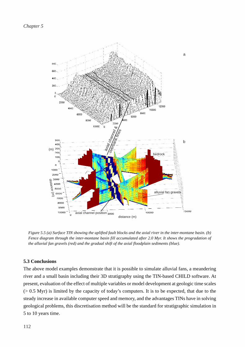
5.2.3 Basin fill

The last example of a modelled stratigraphy is of relatively large temporal and spatial scale for a

CHILD simulation (10 x 10 km, 40 x 40 nodes, simulation time ~ 2.0 Myr, Figure 5.5). The modelled

setting consists of a depositional basin confined by two uplifting fault blocks. The fault blocks are

eroded and deliver two grainsize fractions to the small inter-montane basin. During the steepest

descent routing of the sediment into the basin the sediment carried by the flow is sorted using the

two-fraction model of Wilcock (1998). An extra sediment source is entering the basin in the form of

an axial flowing river, which is instructed to spread fine-grained floodplain sediments (blue). Initially

the river occupies the centre of the intermontane basin, but its position gradually shifts by the

progradation of the right-hand side alluvial fans (Figure 5.5).

110

Chapter 5

T = 500 yr

T = 1000 yr

T = 1500 yr

T = 2000 yr

T = 2500 yr

T = 3000 yr

T = 3500 yr

T = 4000 yr

T = 4500 yr

T = 5000 yr

base levellowering

base levellowering

Figure 5.3 Simulation of a meandering river depicted in successive timesteps of 500 yrs. Intervals of meanderingand alluviation of the valley correspond to phases of base-level rise, while straightening by incision occurduring base-level fall (t=2000 and t=4000 yrs).

111

CHILD

deposit age (yrs)

fluvial path

4500

4000

3500

3000

2500

2000

1500

1000

500

0

60

40

20

0

elev

atio

n(m

)

100 200 300 400500 600 700 800 900 1000distance (m)

10

5

0

-5

800

600

550

500

450distance (m)

Figure 5.4 TIN representation the floodplain occupied by the meandering channel. The TIN is made transparentin order to visualize three stratigraphic sections of the floodplain subsurface. The sections are coloured accordingto the depositional age of the strata, showing older sediment at the sides of the valley as fluvial terraces, andyounger strata occupying the valley centre.

112

Chapter 5

5.3 Conclusions

The above model examples demonstrate that it is possible to simulate alluvial fans, a meandering

river and a small basin including their 3D stratigraphy using the TIN-based CHILD software. At

present, evaluation of the effect of multiple variables or model development at geologic time scales

(> 0.5 Myr) is limited by the capacity of today’s computers. It is to be expected, that due to the

steady increase in available computer speed and memory, and the advantages TINs have in solving

geological problems, this discretisation method will be the standard for stratigraphic simulation in

5 to 10 years time.

Figure 5.5 (a) Surface TIN showing the uplifted fault blocks and the axial river in the inter-montane basin. (b)Fence diagram through the inter-montane basin fill accumulated after 2.0 Myr. It shows the progradation ofthe alluvial fan gravels (red) and the gradual shift of the axial floodplain sediments (blue).

axia

l cha

nnel

&

over

bank

fine

s

alluvial fan gravels

bedrock

a

b

distance (m)

distance (m)

(m)

axial channel position