1

Stratospheric ozone and Southern

Hemisphere climate change:

Impacts and robustness in CMIP5 models

Helen Sanderson

MSc Research Project

A dissertation submitted to Lancaster University for the degree Master of Science (by

research) in Environmental Science within the Lancaster Environment Centre.

2

Acknowledgments

I wish to thank my supervisor Paul for all his advice and always responding to my queries even if he

was on the other side of the Atlantic. I would also like to thank my friends and family, especially to

Nickie, Nando and Hasifah in the office for their guidance and coding advice, to Leyla and Adam their

encouragement and to Ollie for his support and endless patience. This accomplishment would not

have been possible without them.

3

Abstract

Stratospheric ozone depletion is thought to be the dominant cause of recent observed southern

hemisphere (SH) circulation changes during austral summer, along with the consequential impacts

on tropospheric climate conditions. Links between ozone depletion and the positive phase of the

dominant mode of variability of the southern annular mode (SAM) have been found, which in turn

are linked to changes in precipitation, atmospheric temperatures and winds. This dissertation

investigates how well the models from the most recent Coupled Model Intercomparison Project

(CMIP5) represent these changes and searches for consistencies and differences across the models.

Comparisons are made with the reanalysis data set ERA-Interim. It is found that the magnitudes of

the model trends vary dramatically across the CMIP5 ensemble, although between 1960-2000 all

models have decreasing austral spring stratospheric ozone and November temperatures and

increasing austral summer SAM trends. Across the CMIP5 models, the strength of the SAM trend is

only loosely related to the strength of the stratospheric ozone trend, and this relationship does not

always hold. There are changes in precipitation and surface temperatures that are significantly

related to the SAM, with bands of increasing and decreasing trends across the SH, likely as a result of

the poleward shift in storm tracks. However the magnitude and location of regional changes in

surface climate that can be attributed to the SAM differ considerably across the models. For

correlations of the SAM with both precipitation and surface temperatures, the models under-

estimate the correlation over southern Africa and are relatively good representations of Antarctica

when compared to reanalysis data.

4

Table of Contents

1. Introduction ....................................................................................................................... 5

1.1 Stratospheric ozone ............................................................................................. 5

1.2 Changes in circulation ..........................................................................................

1.3 Changes in climate ...............................................................................................

2. Data and Methodology.......................................................................................................

2.1 CMIP5 models ......................................................................................................

2.2 ERA-Interim ..........................................................................................................

2.3 Variables investigated in this study ......................................................................

3. Trends in stratospheric ozone and direct consequences ...................................................

3.1 Stratospheric ozone, temperature and SAM trends .............................................

3.2 Comparing trends ................................................................................................

4. Trends in Southern Hemisphere tropospheric climate ......................................................

4.1 Correlations between the SAM and climate variables ..........................................

4.2 Impacts on precipitation and surface temperature ..............................................

5. Is the SAM in CMIP5 models and ERA-Interim statistically indistinguishable? ...................

5.1 Creating rank histograms .....................................................................................

5.2 CHEM model rank histograms ..............................................................................

5.3 CMIP5 model rank histograms .............................................................................

6. Discussion ...........................................................................................................................

7. Summary and Conclusions .................................................................................................

Appendix ................................................................................................................................

References .............................................................................................................................

5

5

8

9

13

13

16

17

19

19

22

26

27

29

37

37

39

41

44

49

53

55

5

Chapter 1: Introduction

Observations of stratospheric ozone levels show a clear decrease in total ozone abundance from

around the 1970s to the early 2000s, driven by anthropogenic emissions of ozone depleting

substances (ODSs) such as chlorofluorocarbons (CFCs) [Solomon 1999, WMO 2014]. A strongly

seasonal ozone hole (an area of substantial decreases in ozone) has formed in the stratosphere over

Antarctica every austral spring, first reported by Farman et al [1985]. Stratospheric ozone depletion

is thought to be the dominant cause of recent observed changes to stratospheric temperatures and

tropospheric circulation in austral summer in the southern hemisphere (SH), a poleward shift and

strengthening of the SH mid-latitude jet stream and the positive trend in the southern annular mode

(SAM, which describes the north-south movement of the westerly wind belt) during austral summer

[Son et al. 2010, Polvani et al. 2011, IPCC 2013, Bandoro et al. 2014, Previdi & Polvani 2014, WMO

2014, Young et al. 2014]. These shifts in the jet stream have led to changes in tropospheric climate in

the SH during austral summer [Hendon et al. 2007, Thompson et al. 2011, Purich and Son 2012,

Gonzalez et al. 2013, Previdi & Polvani 2014, WMO 2014]. Observational [Hendon et al. 2007,

Thompson et al. 2011, Bandoro et al. 2014] and model studies [Kang et al. 2011, Fyfe et al. 2012,

Purich and Son 2012, Gonzalez et al. 2013] have explored how stratospheric ozone depletion and

recent changes in SH climate are linked. There have been multi-model studies covering all of the SH

[Fyfe et al. 2012, Purich and Son 2012], and regional scale studies with only a few models [Kang et al.

2011], but few multi-model studies on regional scales. As a result, this project has the central aim of

investigating how robust climate models are in showing how stratospheric ozone depletion relates

to regional changes in surface climate in the SH, exploring model differences.

1.1 Stratospheric ozone

The stratosphere, where the vast majority of ozone depletion has occurred, describes the region of

the atmosphere from approximately 12km up to 50km, where - in contrast to the troposphere below

- temperatures increase with height due to ozone absorbing incoming solar radiation. As ozone

concentrations peak in the stratosphere, the absorption of solar radiation in the stratosphere

prevents ultraviolet (UV) radiation reaching the Earth's surface [Jacob 1999]; excessive doses of UV

in the troposphere can be harmful and cause skin damage [EEAP 2014]. Ozone is also present in the

troposphere, where its capacity as a greenhouse gas (GHG) peaks and where it is a harmful pollutant

for humans, animals and plants [Finlayson-Pitts and Pitts 1997, Karnosky et al 2006].

6

Figure 1: How ozone levels change with altitude in the tropics. From WMO's twenty questions and

answers about the ozone layer (2014, their figure for Q1-2)

During the second half of the twentieth century, rapid stratospheric ozone depletion was detected in

observations [reviewed by Solomon 1999]. The most extreme depletion occurs in austral spring

(September, October, November, or SON) in the Antarctic stratosphere, where the particular

chemical and meteorological conditions can result in near total depletion at some altitudes, forming

the ozone hole [Farman et al. 1985, Solomon 1999, WMO 2011, Previdi and Polvani 2014, Solomon

et al 2014]. The lack of land mass in the SH leads to a more constant, stable jet as land-ocean

temperature contrasts are less and there are fewer mountains (which can deflect energy, causing

the jet stream to meander). These conditions encourage a cold isolated polar vortex to form over

the Antarctic, which allows for the formation of polar stratospheric clouds (PSCs), which greatly

accelerate ozone destruction at polar sunrise in the austral spring [Solomon 1999]. Greater ozone

depletion is seen in years with a colder, longer lasting vortex [Parrondo et al. 2014, Solomon et al.

2014], linked to the ability of ozone destruction itself to cool the stratosphere and prolong the

vortex lifetime [Waugh et al. 1999]. Temperatures in the Arctic stratosphere do not generally reach

the same low levels and hence ozone depletion is not as great [Solomon 1999].

7

Figure 2: The vertical distribution of Antarctic and Arctic ozone for years with and without strong

stratospheric ozone depletion. The total ozone values can be seen in the parentheses. From WMO's

twenty questions and answers about the ozone layer (2014, their figure for Q12-3)

The issue of decreasing stratospheric ozone levels is important as there is evidence that human

emissions of ODSs is the main driver of this depletion [Solomon 1999]. ODSs such as CFCs are long-

lived compounds that only break down when they reach the stratosphere, where they are

photolysed by high energy UV photons releasing chlorine atoms, which catalytically destroy

stratospheric ozone [reviewed by Solomon 1999]. Less ozone in the stratosphere means more UV

radiation reaches the Earth's surface [WMO 2011], leading to damage to ecosystems [EEAP 2014] as

well as impacting on the climate.

Another impact of this loss of ozone is a resultant stratospheric cooling trend (as ozone heats the

stratosphere) particularly in the lower stratosphere [Shine et al. 2003, Randel et al. 2009, WMO

2011, IPCC 2013]. This cooling has been observed over much of the globe, with around a 0.5 K/dec

cooling in the stratosphere between 1979 and 2007 [Randel et al. 2009]. The largest cooling has

been observed in austral spring and summer in the Antarctic lower stratosphere (up to 3.5 K/dec)

[Randel et al. 2009, Young et al. 2013], with model simulations representing this trend well [Shine et

8

al. 2003, Young et al. 2013]. While increases in GHGs have also contributed to stratospheric cooling

[Polvani et al. 2011, Fyfe et al. 2012], this large, seasonal Antarctic cooling is primarily a result of

ozone depletion [Randel et al. 2009].

1.2 Changes in circulation

Comparatively recently, observation [e.g. Thompson and Solomon, 2002] and model [Gillett and

Thompson 2003, Polvani et al. 2012] studies have shown that changes in temperature and ozone

levels in the Antarctic stratosphere are a major driver of SH tropospheric climate change. These

changes in climate result from changes in circulation [Gerber and Polvani 2009, Previdi and Polvani

2014], although the exact driving mechanism is as yet unknown [WMO 2014]. It is known that as

Antarctic polar vortices are very cold, a latitudinal pressure gradient that forms between the pole

and mid-latitudes; along with the Earth's rotation, this creates a belt of westerly winds. Wind speeds

can exceed 100 ms-1 [Schoeberl and Hartmann 1991, Solomon 1999, Previdi and Polvani 2014].

Cooler stratospheric temperatures as a result of ozone depletion coincide with increases in the

meridional temperature gradient between the pole and mid-latitudes and an increase in the vertical

changes of atmospheric winds, which in turn manifests as a strengthening of the band of westerly

winds encircling the pole [reviewed by Previdi and Polvani 2014]. There has also been a significant

strengthening of the SH Brewer-Dobson circulation (tropics to pole circulation in the stratosphere)

during August through to the mid-stratosphere, although it is not clear if this is linked to the ozone

hole [Young et al. 2012].

Poleward shifts in the tropospheric jet are also associated with a stronger polar vortex [Thompson

and Solomon 2002, Gerber and Polvani 2009]. Changes in the strength of the SH polar vortex are

followed by similarly signed changes in the tropospheric circulation that can last for more than two

months [Thompson et al. 2005]. Observations and model studies show that there has been a

poleward shift and strengthening of the SH mid-latitude jet stream in response to changes in the

stratosphere related to ozone depletion [McLandress et al. 2011, IPCC 2013, Gerber and Son 2014,

Previdi and Polvani 2014]. The impact of the poleward jet shifts may also be seen in the widening of

the SH branch of the Hadley circulation (equator to sub-tropics circulation in the troposphere),

extending the ozone hole's climate impacts into the subtropics [Polvani et al. 2011]. The largest

tropospheric response, for example the largest shifts in the jet stream, are in the austral summer

[McLandress et al. 2011, Barnes et al. 2014].

9

These stratospheric ozone driven changes in circulation reflect the positive phase of the SAM

[Thompson et al. 2005], which is the major mode of climate variability in the SH [Thompson and

Wallace 2000]. The phases of the SAM describe the north–south movement of the westerly wind

belt around Antarctica, with a positive phase illustrating a poleward shift in the wind belt. Over the

latter half of the twentieth century, it has been found that changes in stratospheric ozone levels is

the most significant driver of shift in the SAM, with the strongest correlations occurring during

austral summer and autumn [Arblaster and Meehl 2006, Roscoe and Haigh 2007].

Observational [Thompson and Solomon 2002, Marshall 2003] and model studies that examined the

climate role of the ozone hole [Polvani et al. 2011, Gillett and Fyfe 2013] all point to a positive trend

in the SAM since approximately the 1960s, which begins to level off in the last decade, likely due to

less stratospheric ozone depletion occurring around this time [Fyfe et al. 2012]. In addition to the

relationships between stratospheric ozone loss and the SAM on long time scales, more recent

studies have suggested that the magnitude of the ozone hole could be used for seasonal prediction,

since there is a relationship between September ozone concentrations and the subsequent October

SAM index [Son et al. 2013, Bandoro et al. 2014].

1.3 Changes in climate

The SAM also impacts many climate parameters in the SH. Several model [Kang et al. 2011, Fyfe et

al. 2012, Purich and Son 2012, Gonzalez et al. 2013], reanalysis [Manatsa et al. 2013, Bandoro et al.

2014] and observational [Hendon et al. 2007, Thompson et al. 2011, Bandoro et al. 2014] studies

have suggested that Antarctic ozone depletion may have impacted recent regional surface climate

change in austral summer (December-February, which will be referred to as DJF in this study),

implying that stratospheric variability is a driver of surface climate variability [Thompson et al. 2005].

Climate impacts of the SAM are also consistent with and follow variations in the stratospheric polar

vortex, for example changes in surface temperatures throughout much of Antarctica [Thompson et

al. 2005].

Studies have shown that there have been changes in austral summer precipitation most likely to do

with anthropogenic rather than natural forcings, especially as a result of stratospheric ozone

depletion [Timbal et al. 2006, Kang et al. 2011, Fyfe et al. 2012, Purich and Son 2012, Gonzalez et al.

10

2013]. In general, there has been drying in the mid-latitudes and increased precipitation in the high-

latitudes and the sub-tropics of the SH, over a time period of around 1960 to 2010 [Kang et al. 2011,

Fyfe et al. 2012, Purich and Son 2012, Previdi and Polvani 2014]. This zonal structure of precipitation

can at least in part be explained by circulation changes in the atmosphere (for example the SAM)

and is most likely a result of the poleward shift of the tropospheric mid-latitude jet and storm tracks

[Gillett et al 2006, Previdi and Polvani 2014]. Observations of precipitation near 10oS are not well

reproduced by stratospheric ozone forced models, so it is likely that the strong decreases in

precipitation here are not a result of ozone forcing [Previdi and Polvani 2014].

Distribution and strength of rainfall proves to be complex in terms of prediction as precipitation

changes are often sporadic due to the nature of how precipitation forms, and it is well known that

precipitation can be highly model dependent. Purich and Son [2012] found that whilst extreme

precipitation events are not sensitive to ozone depletion, DJF precipitation trends (light precipitation

1-10mm day-1) in the SH extra-tropics are significantly affected by Antarctic ozone forcings.

Trends in precipitation related to changes in the SAM are also highly regional. Observed austral

summer precipitation trends over much of Australia include increases for the south-east coast and

drying in the west of Tasmania [Gillett et al. 2006, Hendon et al. 2007], with changes in the SAM

accounting for around 15% of the 1979-2005 trend [Hendon et al. 2007]. Timbal et al. [2006] found

that the observed drying in south-west Australia since the mid-1960s was best explained by trends in

GHGs and aerosols, and stratospheric ozone depletion. For New Zealand, it is thought that the

trends in the SAM account for 80% of the observed austral summer precipitation [Gillett et al. 2006,

Ummenhofer et al. 2009], which include drying of both islands in the south and west, and increased

precipitation in the east, related to the shifting storm track associated with the SAM. Ozone

depletion-driven trends in the SAM have also been implicated in DJF rainfall increases in south-east

South America [Gonzalez et al., 2013], as well as drying over southern South America and increased

rainfall over South Africa [Gillett et al., 2006].

Ozone hole driven trends in austral summer surface temperatures also vary from region to region. In

general, austral summer tropospheric cooling over the Antarctic has been observed [Thompson and

Solomon 2002, Gillett et al. 2006, Johanson and Fu 2007] in late twentieth century, which has been

reproduced in climate models [McLandress et al. 2011]. More specifically, there have been increases

in surface temperature over the Antarctic Peninsula, with similar strength cooling over parts of East

Antarctica [Thompson and Solomon 2002, Previdi and Polvani 2014], with around half of this

11

warming in the Antarctic Peninsula and most of the cooling over East Antarctica congruent to the

SAM [Thompson and Solomon, 2002]. Model simulations forced only by stratospheric ozone

depletion represent observations of warming and cooling over Antarctic regions well [McLandress et

al. 2011].

Cooler summer temperatures have been observed over the southeast and south-central Australia

[Bandoro et al. 2014], along with cooler maximum summer temperatures for central and eastern

subtropical Australia associated with the positive phase of the SAM [Hendon et al. 2007]. Austral

summertime warming in Tasmania and in the south of New Zealand are also thought to be linked to

the SAM [Gillett et al. 2006, Hendon et al. 2007]. Southern America has seen warming over

Patagonia and Argentina, of which much can be explained by the SAM [Gillett et al. 2006, Thompson

et al. 2011, Previdi and Polvani 2014]. Areas of Africa where the SAM coincided with the Angola low

have more pronounced links between the ozone hole and surface air temperatures, with austral

summer cooling in the south west of southern Africa and warming further north in southern Africa

[Manatsa et al. 2013]. Yet station and reanalysis data point towards decreasing surface

temperatures in austral summer over inland areas of the southern tip of Africa [Bandoro et al. 2014].

Figure 3: (Left) Trends from December to May; (right) the contribution of the SAM to the trends.

Coloured circles represent linear trends from 1969 to 2000 of surface temperature, with a contour

interval of 0.5 K per 30 years. Vectors represent linear trends from 1979 to 2000 of 925 hPa winds,

with the longest vector corresponding to around 4 ms−1. From Thompson and Solomon (2002; part

of their Figure 6)

12

There are also SAM driven trends outside of austral summer, such as observed changes in austral

winter precipitation in the last 50 years over parts of Australia, including dryer conditions over parts

of southern Australia associated with the SAM [Meneghini et al. 2007, Delworth and Zeng 2014].

Also, austral winter and spring surface warming of a larger scale over Antarctica have been observed

[Johanson and Fu 2007], which along with observed austral summer and autumn cooling over the

Antarctic indicates that there are seasonal changes in tropospheric circulation, reflecting the

seasonality of stratospheric ozone depletion [Previdi and Polvani 2014]. However this dissertation

only explores austral spring and summer tropospheric relationships with the SAM as the impact of

ozone depletion is considered strongest in austral summer.

In general, it must be remembered that changes in surface temperature and precipitation in the SH

cannot all be attributed to the ozone hole as several other factors, such as the El Niño-Southern

Oscillation (ENSO) and increases in GHGs, influence regional climate change. It is suggested that

changes in circulation are a dominant driver of climate change in some areas of the SH, but other

factors do also influence changes in the atmosphere [Previdi and Polvani 2014].

In this study, output from a large ensemble of climate models is used with the aim of exploring the

robustness of historical simulations of stratospheric and tropospheric conditions in the SH before

2005. Historical studies are useful as they can be compared with observations, unlike projections

into the future, and although there will always be errors in climate model output, they are useful in

gaining understanding of climate systems. It is also advantageous to use a large number of models

so that their similarities and differences can be explored, which is useful in evaluating how much

faith should be put into regional studies only using a small number of climate models.

This study builds on previous multi-model studies [Fyfe et al. 2012, Eyring et al. 2013, Gillett and Fyfe

2013, Young et al. 2014] by investigating the robustness of ozone-driven regional climate changes

across CMIP5 models (with a focus on several chemistry-climate models) [Son et al. 2013, Bandoro

et al. 2014]. These models are also compared to the reanalysis data set ERA-Interim. The climate

models and data analysis methods are described in Section 2. Section 3 reports the trends in

stratospheric ozone, stratospheric temperatures and the SAM across the CMIP5 models, as well as

discussing model differences, Section 4 presents analysis of regional trends in tropospheric climate

related to the SAM, and Section 5 uses rank histograms to determine how well the models portray

changes in the SH. These results are discussed in Section 6 and the overall conclusions are

summarised in Section 7.

13

Chapter 2: Data and Methodology

2.1 CMIP5 models

This study investigates historical simulation output from models used in the CMIP5 (Coupled Model

Intercomparison Project phase 5) experiment [Taylor et al. 2012], in support of the

Intergovernmental Panel on Climate Change (IPCC) in the Fifth Assessment Report (AR5) in 2013

[IPCC 2013]. The Working Group on Coupled Modelling (WGCM) of the World Climate Research

Programme (WCRP) endorsed CMIP5, and for model development there was a focus on improving

knowledge of areas of past and future climate changes that are less understood [Taylor et al. 2012].

Previously, there have been multi-model studies that have analysed hemisphere scale changes, and

single model studies assessing regional changes, but how robust these changes are in climate model

ensembles on regional scales has not yet been thoroughly explored, which creates a focus for this

study.

Whilst these CMIP5 historical simulations cover the period 1850-2005, the analysis focuses on the

years between 1960-2000, similar to the work of Previdi and Polvani [2014]. The greatest change in

stratospheric ozone levels occurred during this time period, and stratospheric chlorine levels peaked

in 2000 [Newman et al. 2007]. This analysis is confined to the SH as it is concerned with the climate

impacts of the Antarctic ozone hole.

The CMIP5 models used in this study are stated in Table 1 [using information from Eyring et al.

2013]. Some of the CMIP5 simulations have more than one realisation of the historic climate, and in

these cases the first ensemble member is taken, so as not to bias the results to a particular model.

Further individual model details can be found in Eyring et al. [2013, and references therein] and

Shindell et al. [2013] for the GISS models.

As ozone is included in CMIP5 models in different ways, ozone depletion will vary from model to

model, as will climate impacts. A grouping system is used to segregate output from models with and

without interactive chemistry. Those with interactive chemistry are referred to as 'CHEM' models.

Another group is 'semi-offline', which use prescribed ozone data sets that are calculated by a

related CMIP5 chemistry-climate model, with stratospheric ozone responding to changes in GHG

concentrations [Eyring et al. 2013]. The final group is 'prescribed', which refers to those models

using prescribed ozone data sets. Many in this group use a time-varying ozone database, without

14

interactive chemistry, known as the AC&C/SPARC (Atmospheric Chemistry and Climate/Stratospheric

Processes and their Role in Climate) ozone database [Cionni et al. 2011], which shall be referred to

as 'SPARC' for the remainder of this study. The store of data used did not have any saved ozone data

for some of these SPARC models, despite Eyring et al. [2013] stating that they used ozone data from

this database. As a result, for the SPARC models that did not have their ozone data archived, the

ozone output from BCC-CSM1-1 (the model with data closest to the mean and median of the saved

SPARC ozone data) was used.

Table 1. Details of the CMIP5 models and their ozone. Models are split into groups of how ozone is included:

chemically interactive (CHEM), semi-offline, and prescribed ozone data sets (PS, PG and PM). Abbreviations are

described in the table endnotes.

Modelling Centre and address Model Group

Centre for Australian Weather and Climate

Research, Australia

ACCESS1-0

ACCESS1-3

PS

PS

Beijing Climate Centre, China

Meteorological Administration, China

BCC-CSM1-1

BCC-CSM1-1-m

PS

PS

College of Global Change and Earth system

Science, Beijing Normal University, China

BNU-ESM

Semi-offline

National Centre for Atmospheric

Research, USA

CCSM4

Semi-offline

Community Earth System Model

Contributors

CESM1-BGC

CESM1-CAM5

CESM1-FASTCHEM

CESM1-WACCM

Semi-offline

Semi-offline

CHEM

CHEM

Centro Euro-Mediterraneo per I

Cambiamenti Climatici, Italy

CMCC-CM

PS

Centre National de Recherches

Meteorologiques, France

CNRM-CM5

CHEM

15

Commonwealth Scientific and Industrial

Research Organization in collaboration with

Queensland Climate Change Centre of

Excellence, Australia

CSIRO-Mk3-6-0

PS

EC-EARTH consortium, Europe EC-EARTH PS

LASG, Institute of Atmospheric Physics,

Chinese Academy of Sciences and CESS,

Tsinghua University, China

FGOALS-g2

PS

NOAA Geophysical Fluid Dynamics

Laboratory, USA

GFDL-CM3

GFDL-ESM2G

GFDL-ESM2M

CHEM

PS

PS

NASA Goddard Institute for Space Studies,

USA

GISS-E2-H

GISS-E2-H-CC

GISS-E2-H-p2

GISS-E2-H-p3

GISS-E2-R

GISS-E2-R-CC

GISS-E2-R-p2

GISS-E2-R-p3

PG

PG

CHEM

CHEM

PG

PG

CHEM

CHEM

Met Office Hadley Centre, UK

HadCM3

HadGEM2-CC

HadGEM2-ES

PS

PS

PS

National Institute of Meteorological

Research, Korea Meteorological

Administration, Korea

HadGEM2-AO

PS

Russian Institute for Numerical

Mathematics, Russia

INMCM4

PS

16

Institut Pierre Simon Laplace, France

IPSL-CM5A-LR

IPSL-CM5A-MR

IPSL-CM5B-LR

Semi-offline

Semi-offline

Semi-offline

Japan Agency for Marine-Earth Science and

Technology, Atmosphere and Ocean

Research Institute (The University of

Tokyo), and National Institute for

Environmental Studies, Japan

MIROC4h

MIROC5

MIROC-ESM

MIROC-ESM-CHEM

PM

PM

PM

CHEM

Max Planck Institute for Meteorology,

Germany

MPI-ESM-LR

MPI-ESM-P

PS

PS

Meteorological Research Institute, Japan

MRI-CGCM3

PS

Norwegian Climate Centre, Norway

NorESM1-M

NorESM1-ME

Semi-offline

Semi-offline

PS: AC&C/SPARC [Cionni et al. 2011]; PG: data set described by Hansen et al. [2007]; PM: data set described by Kawase et al.

[2011].

2.2 ERA-Interim

To ground the CMIP5 historic simulation outputs, ERA-Interim reanalysis data is used. This is a global

atmospheric data set starting from 1979 - due to vast improvements in satellite data collection - that

is continuously updated. As a result, ERA-Interim data used in this study covers the years 1979 to

2000. This data set uses both forecast models and data assimilation where the atmosphere, ocean

waves and land-surface are included and there is a spatial resolution of approximately 80 km on 60

vertical levels (ranging from the surface to 0.1 hPa) [more details can be found in Dee et al. 2011]. It

is assumed that this data set is closer to reality than that of the models.

Merits of ERA-Interim (when compared to ERA-40 which was completed in 2002) include improved

representation of stratospheric circulation and the hydrological cycle, although there is still room for

further progress [Dee et al. 2011]. Although ERA-Interim may under-estimate Antarctic lower

17

stratospheric cooling as a result of ozone depletion by a factor of 2 compared to IGRA (Integrated

Global Radiosonde Archive) radiosonde observations, the inter-annual variability of these

temperatures is large enough that the differences between the trends are still within statistical

uncertainty [Calvo et al. 2012]. Also, ERA-Interim climatology has been found to be very similar to

radiosonde climatology [Wenzel et al. 2015], hence the use of this re-analysis data set as a basis for

'real life' in this study.

2.3 Variables investigated in this study

The relationship between stratospheric ozone depletion and climate change is examined in this

study using CMIP5 models and ERA-Interim data. For the following analysis, the term 'column ozone'

refers to the zonal mean of column ozone (1000-10hPa) over the polar cap (65°S to 90°S). This will

be seasonal data, refined to the austral spring months September, October and November (SON)

due to the greatest ozone depletion being observed during austral spring every year [Son et al. 2008,

Previdi and Polvani 2014]. The column ozone data is in Dobson Units and often was normalised to

1980 so that different initial values between the models have less of an impact on trend

comparisons.

Another variable used is stratospheric temperature. This is taken at 70hPa as the greatest trends

from 1960 to 2000 can be seen here in the CMIP5 data. November has been shown in studies [Young

et al. 2013] to be the month with the greatest decrease in stratospheric temperature, hence

stratospheric temperature data is restricted to this month only, and has units of degrees Kelvin.

The SAM index can be calculated in various ways, including using sea level pressure as in Gong and

Wang [1999], Marshall [2003] and Gillett and Fyfe [2013], which is the method used in this study.

The pressure at sea level (PSL) at 40°S and 65°S are imputed into the equation

SAM index = (PSL40S - 40S) - (PSL65S -

65S)

with units of hPa, where PSL40S and PSL65S are the PSL measurements at their given latitude, and

stands for the zonal mean at a given latitude. This is a straightforward and physically meaningful way

to calculate the SAM compared to other methods [Previdi and Polvani 2014]. Gong and Wang [1999]

chose these latitudes because of the statistical significance and the strength of the correlation

18

coefficient between them. The SAM index has been calculated for the austral summer months (DJF)

as impacts on SH climate have been found to be most pronounced here [Gillett and Fyfe 2013],

meaning there is a delay between stratospheric ozone depletion and climate impacts. All the SAM

data has been normalised to 1980.

Throughout this study when any of tropospheric climate variables studied (sea level pressure, mid-

tropospheric winds, temperature and precipitation) are analysed, they will be averaged for DJF

(unless otherwise stated). When column ozone data is compared to the SAM, the DJF will be taken

directly after the relevant SON, so for example 1980 SON data will be compared to 1980 December

and 1981 January and February data.

19

Chapter 3: Trends in stratospheric ozone and direct consequences

This section will present analysis of stratospheric ozone, stratospheric temperature and SAM trends

between 1960 and 2000 using output from the 43 CMIP5 models, with a particular emphasis on how

robust the findings are across the models. Stratospheric ozone depletion is known to cause

stratospheric temperature decreases, which is thought to be related to positive trends in the SAM

index. The results in this section confirm the work of others [such as Previdi and Polvani 2014] and

are to provide context for later sections of this study.

3.1 Stratospheric ozone, temperature and SAM trends

Figure 4 shows the time series of SON column ozone, November stratospheric temperature and the

DJF SAM for all the CMIP5 models used, with the multi-model means marked in blue and red. The

multi-model mean trend of ozone levels has the highest significance, with stratospheric temperature

slightly weaker and the SAM having the lowest significance. However all three multi-model mean

trends are significant at the 5% level, which is not unexpected as noise in the results is likely to be

cancelled out by studying such a large model ensemble. As multi-model means can mask key

features of individual model trends, especially in such a large group of models, the maximum and

minimum values out of all the models for each year are plotted. This illustrates the spread of the

model output.

Figure 4(a) illustrates how the dramatic decrease in stratospheric ozone above the Antarctic that has

been observed in the last few decades, especially between 1960 and 2000 [Solomon 1999, Parrondo

et al. 2014] is present in the CMIP5 models. The multi-model mean is significant at the 1% level with

a drop of nearly 150DU between 1960 and 2000 and a trend of -40.5 DU/decade. Hence the models

exemplify how remarkable the decline in stratospheric ozone has been, which inspires further

exploration of this data set. This figure also indicates that after the year 2000, stratospheric ozone

levels appear to level out. Hence this study will limit the time period explored to 1960-2000 when

stratospheric ozone depletion was at its greatest.

Despite a 100DU difference between the minimum and maximum points each year in Figure 4(a),

the decline in column ozone between 1960 and 2000 is clearly visible and significant at the 5% level

20

Figure 4: Time series of CMIP5 historical simulation outputs of (a) SON SH polar cap (65oS-90

oS) column

ozone from September 1850 to November 2005 (and the red line spans 1960 to 2000); (b) November polar

cap (65oS-90

oS) stratospheric temperatures at 70hPa between 1960 and 2000; (c) DJF SAM index. All plots

show anomalous results as they are normalised to 1980, and in all plots the shaded region indicates the full

model spread with the multi-model mean in blue.

21

at these extremes. There are many fluctuations in column ozone levels before 1960, but these are

small in comparison to the strong negative trend modelled and observed in recent years.

Stratospheric ozone depletion is associated with stratospheric cooling [Shine et al 2003, Randel et al

2009, Bandoro et al 2014, Previdi and Polvani 2014] and so zonal mean polar cap stratospheric

temperature changes from November 1960 to 2000 are plotted in Figure 4(b). November

temperatures show the maximum cooling in observations at 70 hPa [Young et al. 2012], hence the

use of this pressure here. The significant decrease in the multi-model mean temperature signifies a

cooling in the lower stratosphere between 1960-2000, with a trend of -1.9 K/decade, most likely

caused by stratospheric ozone depletion. This trend is comparable to that found from observations

analysed by Randel et al. [2009] who found that the strongest Antarctic cooling trends over late

austral spring and austral summer to be around -1.0 to -1.5 K/decade between 1979 and 2007 at

similar altitudes. Randel et al. [2009] used a later period which included times when stratospheric

ozone levels had begun to level off, which could explain why these trends were weaker than those

found in this dissertation. Figure 4(b) also shows a model spread of around 10 to 20K throughout the

years studied. In general both the maximum and minimum results from the CMIP5 models show

decreasing trends in stratospheric temperature.

Alongside these decreases in stratospheric ozone levels and temperature, a strong positive trend can

be seen in the time series for the SAM index (Figure 4(c)) which is significant at the 5% level. The

SAM multi-model mean has a trend of 1.0 hPa/decade, which is comparable to the analysis by

Marshall et al. [2003] on observational data between 1958 and 2000, who found a positive SAM

trend of 1.05 hPa/decade in DJF with a 95% confidence interval of ±1.35 hPa/decade (which is very

large and includes negative trends). The SAM has the smallest trend when compared to modelled

stratospheric ozone and temperature changes, but this is not surprising as there are other influences

on the SAM other than changes in the stratosphere. Still, the positive SAM trend corresponds with

the declines in stratospheric ozone and temperature, consistent with the idea that changes in the

SAM have been driven by stratospheric ozone depletion suggested by many others [Thompson et al.

2011, Son et al. 2013, Previdi and Polvani 2014]. There is a wide range of results in Figure 4(c), as

shown by the maxima and minima. Although the models maximum and minimum for each year

generally show a positive trend, the annual variations are large - often with a difference of over 20

hPa.

22

3.2 Comparing trends

As these finding are well supported by other studies [Solomon 1999, Son et al. 2013, Bandoro et al.

2014, Previdi and Polvani 2014], discovering how differences in the models affect these results is of

interest. Using averages, maximums and minimums can limit key features in the data being

considered, so by looking at smaller groups of the CMIP5 models a clearer view of the data can be

found. As a result, the models are grouped with respect to how ozone is included in the model - as

how climate models are created clearly has a large impact on the output they create and, in this

study, ozone levels are of special importance. The groups made using this approach are those that

use interactive chemistry (CHEM), those that use prescribed ozone data sets where the data is

calculated entirely offline and 'semi-offline' models (similar to the work of Eyring et al. [2013] as

stated in Section 2).

For the following results the CMIP5 models have been split into these three groups. Comparisons of

CHEM, semi-offline and prescribed models are made to investigate any influence how ozone is

included in the models could have on model output, as how stratospheric ozone changes are

represented in the models can impact on climate sensitivity [Nowak et al. 2015]. Figure 5 shows the

range of trends of SON stratospheric ozone levels, November stratospheric temperatures and DJF

SAM for the CMIP5 models. Again the results are from 1960 to 2000, with austral spring or summer

data used due to the seasonal nature of these changes in the atmosphere.

Despite the prescribed model group being relatively large (25 members compared to the 9 in both

CHEM and semi-offline), many in this group used the SPARC data set, which results in many similar

ozone values. It can be seen from Figure 5 that the prescribed models have a very small inter-

quartile range for ozone trend data as the majority of the models use SPARC data, with the outliers

being the models using different prescribed ozone data sets. The CHEM models have stronger trends

of ozone depletion than those with prescribed or semi-offline data. This group has the largest

median (-53.4 DU/dec) and a range that covers mostly the larger trends, with the boxplot skewed

towards the larger values. Semi-offline models have the smallest median ozone trend (-26.8

DU/dec), still with a skewed range towards larger trends of ozone depletion.

23

Figure 5: Boxplots showing the spread of the CMIP5 historical simulation trends in both SH polar cap SON

column ozone 1959-1999, November stratospheric temperature at 70hPa 1959-1999 and DJF SAM from

1960-2000, indicating how ozone is included in the models: with interactive chemistry (CHEM), prescribed

and semi-offline ozone.

Similar to changes in stratospheric ozone levels, November stratospheric temperatures only have

decreasing trends between 1960-2000, and this positive relationship between the two variables has

been explored in other studies [Shine et al. 2003, Randel et al. 2009, Son et al. 2008, Young et al.

2014]. CHEM models again have the largest median of -2.12 K/dec and a large range of 8.08 K/dec

covering the largest trends, with two extreme outliers (models CESM1-FASTCHEM and CESM1-

WACCM have much larger negative temperature trends). Semi-offline models form a near symmetric

boxplot with a relatively strong median trend of -1.85 K/dec. Despite semi-offline models having the

smallest stratospheric ozone trends, the prescribed models have the smallest stratospheric

temperature trends. However semi-offline and prescribed models have a very similar range of

stratospheric temperature trends (1.84 and 2.07 K/dec respectively), with the prescribed models

skewed towards smaller trends.

The DJF SAM trends for CHEM and semi-offline models are over a similar range to that of

stratospheric temperatures, both skewed towards smaller trends, with semi-offline models giving

the largest median of the three groups. Here the CHEM models have the weakest median trend of

0.82 hPa/dec, despite having the strongest stratospheric ozone and temperature trends. Although

the prescribed models do not have the smallest median, the group's range covers much lower trend

24

values than the other two groups, including near zero results. Despite the different ranges of SAM

trends for each group, the median values are all very similar.

Comparing the boxplots in Figure 5 shows that the CHEM group contains the models with the largest

stratospheric ozone and temperature trends. Prescribed models have the smallest stratospheric

temperature and SAM trends but no extreme ozone trends. Semi-offline models have in general

weaker ozone trends and yet relatively strong SAM trends.

Figure 6: Scatter plot of the trends of CMIP5 historical simulation output of both stratospheric polar cap

column ozone (SON 1959-1999) and SAM (DJF 1960-2000).

Figure 6 investigates these trends further, showing individual model trends for both SAM and

column ozone. Again, as seen in Figure 5, all CMIP5 SON ozone trends are negative and DJF SAM

trends positive between 1960-2000, supporting the work of a previous multi-model study by Son et

al. [2013], which found a significant negative correlation between observed September ozone

concentration and the October SAM index. Most notably, despite the CMIP5 models that used

prescribed ozone data having similar column ozone trends to each other (as most use the SPARC

ozone data set), there is a wide range of SAM trends for this group. Hence it can be seen that the

strength of the relationship between SAM and ozone trends varies dramatically from model to

model.

25

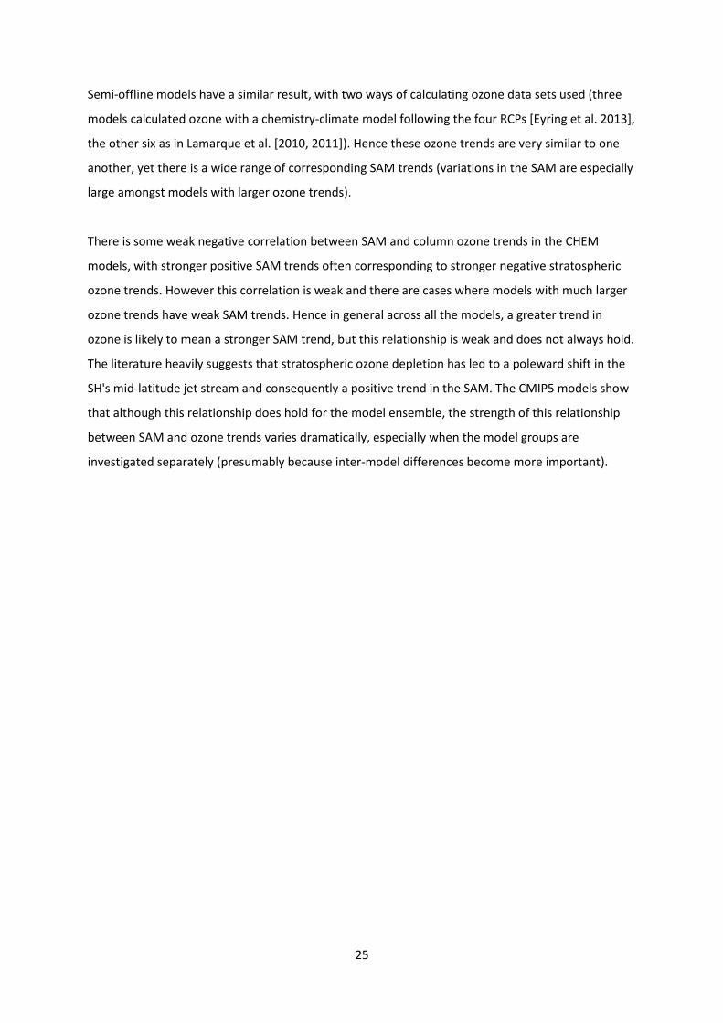
Semi-offline models have a similar result, with two ways of calculating ozone data sets used (three

models calculated ozone with a chemistry-climate model following the four RCPs [Eyring et al. 2013],

the other six as in Lamarque et al. [2010, 2011]). Hence these ozone trends are very similar to one

another, yet there is a wide range of corresponding SAM trends (variations in the SAM are especially

large amongst models with larger ozone trends).

There is some weak negative correlation between SAM and column ozone trends in the CHEM

models, with stronger positive SAM trends often corresponding to stronger negative stratospheric

ozone trends. However this correlation is weak and there are cases where models with much larger

ozone trends have weak SAM trends. Hence in general across all the models, a greater trend in

ozone is likely to mean a stronger SAM trend, but this relationship is weak and does not always hold.

The literature heavily suggests that stratospheric ozone depletion has led to a poleward shift in the

SH's mid-latitude jet stream and consequently a positive trend in the SAM. The CMIP5 models show

that although this relationship does hold for the model ensemble, the strength of this relationship

between SAM and ozone trends varies dramatically, especially when the model groups are

investigated separately (presumably because inter-model differences become more important).

26

Chapter 4: Trends in Southern Hemisphere tropospheric climate

To provide a focus for this project, only the nine CHEM CMIP5 models will be investigated for this

section of the study. Although CMIP5 models in general include higher spatial resolution than CMIP3

and other older models [Taylor et al. 2012], they often still do not include processes such as

atmospheric chemical feedback that is important for representing the climate accurately [Nowak et

al. 2015]. The inclusion of interactive chemistry in the models allows ozone in the models to respond

to climate changes, which is an important step in climate model development as suggested by

Nowak et al. [2015]. This makes them a closer representation of what really happens in the

atmosphere. In contrast, in both prescribed and semi-offline data sets, ozone levels are already set

before the model is run, and so impacts on the current ozone level by atmospheric processes

calculated in the model are not considered.

To help ground CMIP5 model findings, ERA-Interim data is included in this section, covering the

period of 1979-2000. Using reanalysis data alongside the CMIP5 models is useful due to differences

in the models; for example there is a wide spread in DJF austral jet position trends in CMIP5

historical simulations [Gerber and Son 2014]. However as this reanalysis data set begins in 1979 (due

to the use of satellite data) and CMIP5 model analysis will continue to use a time period between

1960 and 2000, when making comparisons with the CMIP5 results, it must always be remembered

that trends from 1960 to 2000 will differ from those from 1979 to 2000. It is assumed that the

relationships between the SAM and tropospheric climate variables are very similar in both time-

scales (as stratospheric ozone declined linearly during both periods of time), but clearly there will be

some differences.

Section 3 discussed hemispheric-scale trends, and to develop these ideas this section investigates

regional-scale trends to see where in the SH is affected. The analysis focuses on how changes in SAM

might affect zonal mid-tropospheric eastward wind (MTW), sea level pressure (PSL), surface

temperature (TAS) and total precipitation rate, firstly at different latitudes due to the zonal nature of

the SAM and then by looking at the entire SH.

27

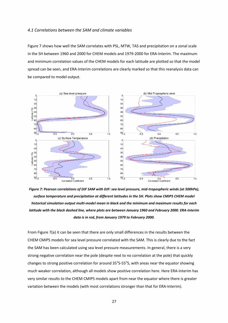
4.1 Correlations between the SAM and climate variables

Figure 7 shows how well the SAM correlates with PSL, MTW, TAS and precipitation on a zonal scale

in the SH between 1960 and 2000 for CHEM models and 1979-2000 for ERA-Interim. The maximum

and minimum correlation values of the CHEM models for each latitude are plotted so that the model

spread can be seen, and ERA-Interim correlations are clearly marked so that this reanalysis data can

be compared to model output.

Figure 7: Pearson correlations of DJF SAM with DJF: sea level pressure, mid-tropospheric winds (at 500hPa),

surface temperature and precipitation at different latitudes in the SH. Plots show CMIP5 CHEM model

historical simulation output multi-model mean in black and the minimum and maximum results for each

latitude with the black dashed line, where plots are between January 1960 and February 2000. ERA-Interim

data is in red, from January 1979 to February 2000.

From Figure 7(a) it can be seen that there are only small differences in the results between the

CHEM CMIP5 models for sea level pressure correlated with the SAM. This is clearly due to the fact

the SAM has been calculated using sea level pressure measurements. In general, there is a very

strong negative correlation near the pole (despite next to no correlation at the pole) that quickly

changes to strong positive correlation for around 35oS-55oS, with areas near the equator showing

much weaker correlation, although all models show positive correlation here. Here ERA-Interim has

very similar results to the CHEM CMIP5 models apart from near the equator where there is greater

variation between the models (with most correlations stronger than that for ERA-Interim).

28

In contrast, the relationship between MTW and the SAM is close to the inverse of that between sea

level pressure and the SAM. Figure 7(b) shows various results in the CHEM models near the pole

(though predominantly negative correlation), very strong positive correlation between 55oS-70oS

which becomes fairly strong negative correlation around 30oS-40oS, with a wide variety of results

near the equator. ERA-Interim in general has a correlation coefficient of 0.5 less than the CHEM

models from the pole to around 40oS, where ERA-Interim data has a peak of negative correlation and

from there to the equator a correlation of around -0.5, becoming weaker nearer the equator. The

changes between positive and negative correlations reflect the poleward shift in the jet stream.

Precipitation and the SAM results from the CHEM models have comparable zonal correlations with

MTW and the SAM, as the shapes of Figures 4(b) and (d) are very similar. There is quite a clear

increasingly positive correlation when moving from the pole to 60oS, strong negative correlation

around 40oS-50oS and a wide range of results towards the equator. The changes between positive

and negative correlations here reflect the poleward shift in the storm tracks. The changes in

correlation are shifted down by around 10oS for correlations with precipitation, at the Earth's

surface, than those for MTW at 500 hPa. There are great similarities between results of ERA-Interim

and CHEM models from the pole to around 50oS, with ERA-Interim showing greater extreme

correlations than the CHEM multi-model mean between 50oS and the equator (especially around

10oS where ERA-Interim has a correlation coefficient of roughly -0.5 and the CHEM multi-model

mean is close to zero). Comparing ERA-Interim MTW and precipitation correlations with the SAM

shows that there is no corresponding positive correlation peak between 20oS-30oS of precipitation in

the MTW. Hence between 40oS and the equator there is no clear pattern between mid-tropospheric

winds and precipitation.

The largest variations between the models are for correlations between TAS and the SAM, with

many changes in correlation of the multi-model mean, hence there is much less confidence in these

results than in the other plots. However Figure 7(c) shows there is the general trend in the CHEM

models of negative correlation from 50oS to the pole, with some positive correlation around 35oS-

45oS, then some negative to no correlation towards the pole. Between 40oS and the pole, these

trends are roughly the inverse of correlations between precipitation and SAM for the same latitudes.

In general, ERA-Interim results have stronger negative correlations and weaker positive correlations

for TAS than the CHEM models multi-model mean, but follow a similar shape across the latitudes.

29

Overall, ERA-Interim results mostly lie within the CHEM CMIP5 model maxima and minima, with the

exception of results for mid-tropospheric wind and near the equator in all plots except Figure 7(a).

There is the least variation between CHEM models in sea level pressure and the most in surface

temperature, with mid-tropospheric winds and precipitation having similar results. Due to

precipitation and surface temperatures having direct impacts on the Earth's surface, they are

investigated further.

4.2 Impacts on precipitation and surface temperature

How these changes in atmospheric composition and properties caused by stratospheric ozone

depletion might be affecting surface climate is an important question. This section will look into

changes in precipitation and TAS, investigating the effect of stratospheric ozone depletion, between

1960-2000, on these surface climate conditions in the SH. Clearly other factors directly impact SH

surface climate as well as stratospheric ozone depletion, such as El Nino and anthropogenic

increases of GHGs, hence it is difficult to distinguish those surface climate changes that are primarily

due to changes in stratospheric ozone levels. As the previous section in this study showed that

decreasing column ozone trends coincide with a positive phase of the SAM - which is also supported

by the literature [Thompson et al. 2005, Previdi and Polvani 2014, WMO 2014] - the relationship

between TAS and precipitation with the SAM is investigated. There are other factors that affect the

phase of the SAM, but stratospheric ozone depletion is thought to be the predominant driver of

shifts in the SAM during this time period. Also, as the SAM is directly linked to changes in the

troposphere, it will have had more direct impact on surface climate than changes in stratospheric

ozone levels.

For further investigation, linearly congruent trends are found, using a similar method to that used in

Thompson and Solomon [2002] and Bandoro et al. [2014]. This is a technique that uses de-trended

signals to find the trend of one variable whilst considering the data of another variable, to create a

more in-depth approach than just comparing the trends of two variables. For the purpose of

explanation, the term TAS is used here although the process is also repeated for precipitation in the

following analysis; both climate variables are restricted to DJF at each location available in the SH.

Following the idea that changes in TAS are due to many factors such as the SAM, GHGs, El Nino and

other natural changes in the atmosphere, how much TAS changes just as a result of the SAM is

30

estimated. To do this, SAM and TAS data are first de-trended, then the trend between SAM and TAS

is multiplied by the SAM trend, using the equation:

where dTASv stands for the estimated change in TAS as a result of changes in the SAM. Plotting these

results shows where the SAM is most likely affecting changes in TAS. To limit correlations occurring

just by chance, the only linearly congruent trends shown are in areas of the SH where the regression

of TAS and SAM is significant at the 5% level. Here the time period used to investigate relationships

of stratospheric ozone depletion and climate change is again between 1960 and 2000 for CHEM

CMIP5 models and 1979-2000 for ERA-Interim data.

Precipitation

Changes in the SAM can alter local precipitation distributions and concentrations. Figure 8 explores

where austral summer precipitation is likely to be increasing and decreasing in the SH, linked to

changes in the SAM. It can be seen that precipitation changes in ERA-Interim are weaker than the

CHEM CMIP5 models in general in the SH. Most of the strong precipitation trends for all of the

models are near the equator and are chaotic. There are little to no trends towards the Antarctic,

with weaker but more consistent trends with a zonal structure of decreasing precipitation trends

north of increasing trends between 30oS to 75oS in general in the CHEM models. ERA-Interim shows

little to no trends in precipitation south of 45oS. In comparison, Kang et al. [2011] used climate

models with reduced polar ozone concentrations and found significant increases in austral summer

precipitation in the southern subtropics (including parts southern Africa, Australia and south eastern

South America) which the study links to a poleward shift of the extratropical westerly jet. They also

found that climate model subtropical precipitation changes between 1979 and 2000 were very

similar to observed patterns.

These findings are supported by Figure 8(b) which shows precipitation changes linearly congruent to

the SAM, where the regression between precipitation and SAM is significant at the 5% level. In

general these plots all show weaker trends than in Figure 8(a), as only the trends likely linked to the

SAM are plotted. The most striking difference between Figures 5(a) and 5(b) is the lack of

precipitation trends near the equator in Figure 8(b). There are still some significant trends in the

tropics, but these are not consistent across the models. Most consistent across the models are the

31

bands of increased and decreased precipitation in the mid to high latitudes, with the increased

precipitation band south of the drying band. These bands reflect the poleward shift in the jet stream.

Figure 8: CMIP5 historical simulation outputs of (a) Trends of austral summer precipitation in the SH; (b)

Trends of austral summer precipitation in the SH with respect to DJF SAM; (c) the correlation between (a)

and (b) just looking at latitudes. All CMIP5 model plots are between January 1960 and February 2000 and

ERA-Interim from January 1979 to February 2000.

32

More specifically, there are few similarities amongst the models and ERA-interim when looking at

the results for the land masses. ERA-Interim only has significant precipitation trends linearly

congruent to the SAM over the west Pacific (as well as very weak increases in precipitation in

southern Africa and decreases over southern South America) but no significant trends in the form of

bands of increased and decreased precipitation across the SH. Most of the CHEM models do show

these bands, but these trends have various strengths across the models. Over Antarctica there is

mostly no change in precipitation linked to the SAM across the models and ERA-Interim, apart from

slight increases in precipitation and decreases associated with SAM on the Antarctic peninsula in a

few of the CHEM models. Some of the CHEM models show increased precipitation over southern

Africa, others have no significant change and one shows a patch of drying in the north of this region.

There are significant changes in Australian rainfall congruent to the SAM, but the strength, location

and sign of these changes varies. Mostly increased trends related to the SAM are in the north, east

and south west, but the exact location of these precipitation increases varies from model to model,

and a few models show drying the north west, over Tasmania and New Zealand. South America has

relatively consistent drying over the southern tip of South America, with generally small areas of

wetter conditions linked to the SAM inland further north.

The latitudinal correlation plots, Figure 8(c), are all very varied with few similarities and many

changes in positive and negative correlation with latitude. Generally the models have the strongest

positive correlations near the pole, or at latitudes corresponding to the bands of increased and

decreased precipitation congruent to the SAM, with most correlations between -0.5 and +0.5 in

strength. ERA-Interim in fact has negative correlation between precipitation trends and precipitation

trends congruent with the SAM at the pole, though it also has its strongest positive correlations just

north of the pole (around 70oS). These positive correlations provide evidence that the modelled and

reanalysis precipitation trends are spatially congruent with the SAM trend zonally near, or just north

of, the pole. The reverse holds such that where there are negative correlations there is evidence that

the changes modelled and reanalysis precipitation are not predominantly due to changes in the SAM

trend for these latitudes (including near the pole in some models), there are most likely other factors

causing these precipitation changes. The correlations get weaker and close to zero near the equator,

suggesting there is no relationship between precipitation changes and the SAM here. These

relationships are in general, with many fluctuations with small changes in latitude.

33

Surface temperature

Figure 9 shows the relationships between austral summer TAS and SAM across the SH from 1960 to

2000 for CHEM models and 1979 to 2000 for ERA-Interim. ERA-Interim uses the temperature 2m

above the surface due to observation methods, and the surface temperature data from the CHEM

models is likely be from equivalent altitudes to that used in ERA-Interim. Overall, ERA-Interim shows

much stronger, predominantly negative changes in temperature, possibly partly because of these

differences, as well as because of differences between modelled and reanalysis data.

Figure 9 shows the relationships between austral summer TAS and SAM across the SH from 1960 to

2000 for CHEM models and 1979 to 2000 for ERA-Interim. ERA-Interim uses the temperature 2m

above the surface due to observation methods, and the surface temperature data from the CHEM

models is likely be from equivalent altitudes to that used in ERA-Interim. Overall, ERA-Interim shows

much stronger, predominantly negative changes in temperature, possibly partly because of these

differences, as well as because of differences between modelled and reanalysis data.

Figure 9(a) shows that in the CHEM CMIP5 models, the majority of the SH has increasing

temperature trends, though again the strength of these positive trends varies dramatically from

model to model. In contrast, ERA-Interim results show mostly cooling temperature trends at 2m

above the surface, with patches of warming such as over the Antarctic Peninsula (which almost

consistently has increasing trends across the nine plots). Thompson and Solomon [2002] also found

warming over the Antarctic Peninsula between 1969 and 2000, with around 0.7 of the ~1.4 K per 32

years warming linearly congruent with the SAM.

If only landmasses are considered, then the models show fairly inconsistent trends in TAS. For

example, GISS-E2-R-p2 shows decreasing TAS trends over much of Antarctica, whereas many other

CHEM models show warming in the similar areas. ERA-Interim results show much more intense

cooling trends over most of Antarctica (apart from the Antarctic Peninsula) which contrasts most of

the CHEM models but supports GISS-E2-R-p2 results over much of Antarctica.

In general, Figure 9(a) shows cooling over parts of southern Africa and warming trends over the rest

of Africa, but the exact location, strength and size of the area that has decreasing TAS trends varies

dramatically. The CHEM models show majority warming trends over almost all of Africa in the SH,

but ERA-Interim only shows warming trends in coastal areas and in the northwest.

34

Figure 9: CMIP5 historical simulation outputs of (a) Trends of austral summer surface temperatures in the

SH; (b) Trends in austral summer surface temperature in the SH linearly congruent with DJF SAM; (c) the

correlation between (a) and (b) just looking at latitudes. All CMIP5 model plots are between January 1960

and February 2000 and ERA-Interim from January 1979 to February 2000.

Trends in TAS over Australia give perhaps the most changeable results across the models, with some

CHEM models showing warming or cooling across the entire country, with most models showing a

mixture of warming and cooling. ERA-Interim shows more intense cooling over most of the country

35

with warming trends in the far west and a band of warming or no change in trends down the centre

of the island. In general, ERA-Interim shows cooling in the south and warming in the north of South

America and the CHEM models have inconsistent cooling and warming across the continent (mostly

warming with small areas of cooling on the central western coast).

Figure 9(b) uses de-trended signals from austral summer SAM and TAS data to find linearly

congruent trends, or in other words the trends in TAS that can be attributed to changes in the SAM.

Only the areas where the regression between TAS and SAM is significant at the 5% level are plotted.

It can be seen that the CHEM models mostly show patches of subtropical warming related to the

SAM over SH oceans with cooling to the north and south of this, with different models portraying

different strength trends. The strongest cooling across the models occurred over parts of Antarctica,

with few to no trends (where the regression of the SAM and TAS is significant at the 5% level) near

the equator. For these general patterns, ERA-Interim results are similar to the models, although the

trends are often much stronger.

There are some regional differences between the reanalysis and model data. Some of the CHEM

models show cooling over southern Africa, whereas ERA-Interim also has warming along the west

coast as well as cooling in the south east of southern Africa. Models show cooling over patches of

eastern and northern Australia and weaker but still significant cooling in the south west, with some

warming seen over New Zealand and south eastern Australia, similar to ERA-Interim results,

although the reanalysis data does show some strong cooling over south west Australia. Patches of

warming, and some cooling, can be seen over southern South America across models and reanalysis

data studied.

Figure 9(c) shows the zonal correlations between Figures 6(a) and (b) for each model and ERA-

Interim data. Most models show little to no correlation at the equator, negative correlation at and

near the pole and mostly weak but positive correlation in between the equator and pole. ERA-

Interim shows near zero correlation at the pole and the equator, weak negative correlation at

around 35°S and positive correlation for the other latitudes, peaking at 65°S with the strongest

correlation seen here. This implies that the modelled and reanalysis TAS trends could be spatially

congruent with the SAM trend zonally between (but not including) the equator and pole. At the pole

for CHEM models and at around 35°S for ERA-Interim, the negative correlation between Figures 6(a)

and (b) suggest that the modelled and reanalysis TAS trends are not due to changes in the SAM (or

other factors over power the effect of the SAM) for these latitudes. When there is near zero

36

correlation showed in Figure 9(c), it implies that these latitudes are not spatially congruent with the

SAM trend here.

37

Chapter 5: Is the SAM in CMIP5 models and ERA-Interim statistically

indistinguishable?

No model is an exact replica of the natural world, but they can still be useful, especially large climate

model ensembles which present a range of outcomes. Model ensembles are said to be truth centred

if reality corresponds to the mean of the model output, such that the model outputs are randomly

distributed with the true climate falling in the centre of the distribution. Alternatively, reality is said

to be statistically indistinguishable from the models if reality could lie anywhere within the model

distribution, and no statistical conclusions could be reliably made. Either way, model ensembles are

useful in determining a spectrum of what has happened in the atmosphere and what is likely to

happen.

5.1 Creating rank histograms

Considering this, it is interesting to explore where the reanalysis data (which uses some

observational data) lies within the CMIP5 model outputs, to determine how well these models

represent the climate. There are drawbacks of comparing CMIP5 models with reanalysis data, such

as the reanalysis data set begins in 1979 and so does not cover the whole time period (1960-2000)

used for CMIP5 data. Similarly to the work of Yokohata et al. [2013], the ERA-Interim data was re-

gridded to the same grid for each of the CMIP5 models for the following analysis.

One way to evaluate and visualise how well the models represent observations (or in this case ERA-

Interim reanalysis data) is to use rank histograms, also known as Talagrand diagrams. This analysis

method has recently been performed with CMIP5 models [Yokohata et al. 2013], where it was

shown that the ensemble represented a range of observations, including surface temperature and

precipitation, relatively well. A model ensemble is considered perfect if the model data is statistically

indistinguishable from the true observed climate variable. However if model data (or reanalysis data)

is consistently either larger or smaller than true observations, then the models are biased away from

reality. If the model data is both generally larger and smaller than observations, the ensemble

spread is too large and the models are said to be over-dispersed (with outputs covering a much

wider range of possible climates than those that actually occur).

38

This section investigates whether the modelled and reanalysis relationships between the SAM and

precipitation or TAS are statistically indistinguishable by using rank histograms (similar to the work

of Annan and Hargreaves [2010] and Yokohata et al. [2013]). This is quantified by comparing the

absolute value of the correlation coefficient between precipitation (or TAS) and the SAM over given

regions of the SH, determining the rank of the ERA-Interim correlation coefficient in a list of CMIP5

plus ERA-Interim data on a grid point by grid point basis. There are limitations of doing this as using

the absolute value doesn't show if the correlation is positive or negative, however if just the

correlation coefficient was calculated and it was a negative value, the smallest value (or any positive

values) would be ranked highest. P-values were also not used as the ERA-Interim data set is over a

smaller number of years, which makes all the p-values larger than those of the CMIP5 models and so

they cannot be compared fairly.

The model (or ERA-Interim) with the weakest correlation coefficient value (not considering whether

this is positive or negative correlation) is given a rank of 1, and the model (or ERA-Interim) with the

largest correlation coefficient has the highest rank. By giving each model and the reanalysis data a

rank, and then plotting ERA-Interim ranks for a set location in the SH gives a visual aid on how well

the models represent the reanalysis data. The shape of these rank histograms can show if the CMIP5

models over-estimate or under-estimate ERA-Interim, and also if the CMIP5 models represent the

reanalysis data well or whether the ensemble is overly broad in contrast to statistically

indistinguishable results.

If ERA-Interim has mostly low ranks, then the rank histogram is skewed (forming an L-shaped

distribution) which means that the CMIP5 models are over-estimating the strength of the

relationship between precipitation or TAS with the SAM. If ERA-Interim has mostly high ranks, then

the CMIP5 models are under-estimating the relationship (forming a reversed L-shaped distribution).

If the models predominantly over-estimate and under-estimate the strength of the relationship

between these climate variables, then a U-shaped distribution forms. If ERA-Interim has a mix of

ranks, mostly of medium strength, then CMIP5 models are said to be over-dispersed (forming a

domed-shaped distribution). If ERA-Interim has an equal share of each rank, then the CMIP5 models

fit the reanalysis data well (forming a uniform, flat distribution) and the two are statistically

indistinguishable.

The following regions are investigated because they are relatively well populated and had the

greatest precipitation and surface temperature changes associated with the SAM in the ERA-Interim

39

data in Figures 5 and 6. Southern Africa is defined to be 15°S-35°S and 10°E-40°E, Australia and New

Zealand as 10°S-50°S and 110°E-180°E, Southern South America as 25°S-55°S and 50°W-75°W and

finally Antarctica as 65°S-90°S and all longitudes.

5.2 CHEM model rank histograms

In Figure 10, only the CHEM CMIP5 models are plotted, as in Section 4. These models are taken to be

the most realistic models so investigating how well they represent ERA-Interim is of interest. The

rank of ERA-Interim's (compared to the CHEM models) absolute values of the correlation coefficients

of the SAM with precipitation and TAS in various areas of the SH can be seen. The ranks of

correlations with the SAM are in blue for precipitation and red for TAS.

Most notably, the CHEM models under-estimate the correlation between SAM and both

precipitation and TAS for Southern Africa. This under-estimation is greater for precipitation, but is

still considerable for TAS. This suggests that the CHEM models do not simulate the influence of the

SAM on precipitation and TAS to the same extent as in the reanalysis data. For Southern South

America, the CHEM models slightly over-estimate the climate variables relationship between TAS

and the SAM, and potentially under-estimate the relationship between precipitation and the SAM,

but this is not as clear as the result of Southern Africa. Hence the CHEM models could exaggerate

the relationship between the SAM and climate variables here, but this is weaker pattern found only

using a small model ensemble size.

Over Antarctica, Australia and New Zealand the CHEM models fit the ERA-Interim correlations

between precipitation and the SAM fairly well, and also between TAS and the SAM over Australia

and New Zealand (it is close to impossible to have an perfectly uniform histogram). This suggests

that the CHEM models represent ERA-Interim data well for these regions of the SH. There could

potentially be some over or under-estimation for Australia and New Zealand, but this would be very

weak and the slightly skewed shapes could well have just arisen from studying a relatively small

amount of models. For TAS and the SAM over Antarctica, there is over-dispersion of the CHEM

models. Although this too suggests good model representation of the reanalysis, it suggests that the

models form a truth centred distribution rather than the reanalysis data being statistically

indistinguishable.

40

Figure 10: Rank histograms for ERA-Interim data with CHEM CMIP5 historical simulations finding the correlations

between SAM with precipitation (blue) or surface temperature (red) trends for various areas of the SH. All CMIP5

model plots are between January 1960 and February 2000 and ERA-Interim from January 1979 to February 2000.

41

5.3 CMIP5 model rank histograms

For Figure 11 the above process is repeated, this time using all 43 of the CMIP5 models. This creates

a larger sample group of models to see if the patterns found for the CHEM models hold across all the

CMIP5 models investigated in this study. Also, using more models gives the results from rank

histograms greater statistical significance. Again ERA-Interim's rank amongst the CMIP5 models for

the absolute values of the correlation coefficients of the SAM with precipitation (blue) and TAS (red)

are plotted.

Yokohata et al. [2013] found that the CMIP5 data set are generally over-dispersed for the 9 climate

variables studied (including precipitation, TAS and sea level pressure), with the observations used in

the study generally having middle ranks. This suggests that in general these models do represent

observations well, and Figure 11 investigates how well these models represent reanalysis regionally.

Due to problems in the data store, there are less models investigated for TAS than precipitation in

Figure 11. If only a few grid points were incorrect, those points in space were not included so as not

to lessen the amount of possible ranks. However if too many grid points were unusable, the models

were not included for this part of the study. Five models had corrupt data that would disrupt the

ranking process if plotted, so they are not included in the TAS rank histograms.

Again the relationship between the SAM and both precipitation and TAS is consistently under-

estimated by the CMIP5 models for Southern Africa. The semi-offline and prescribed models

therefore show similar strength correlations of SAM and these two climate variables to the CHEM

models. For TAS in Southern South America, Australia and New Zealand, there is again a slight over-

estimation of the relationship to the SAM by the CMIP5 models, stronger for Southern South

America, but these patterns are much weaker than for Southern Africa. For precipitation in these

regions there is a much better representation of ERA-Interim in the CMIP5 models, potentially with

some under-estimation. These weak patterns of over or under-estimation by the CMIP5 models

could just be due to chance, or due to how these models portray the impacts of changes in the SAM.

The models represent Antarctica well, especially for correlations between the SAM and

precipitation, with the Antarctic correlations between the SAM and TAS slightly over-dispersed. This

suggests that for the CMIP5 models, the relationship of precipitation to the SAM over Antarctica is

statistically indistinguishable, whereas the relationship between TAS and the SAM in the model

42

Figure 11: Rank histograms for ERA-Interim data with CMIP5 historical simulations finding the correlations

between SAM with precipitation (blue) or surface temperature (red) trends for various areas of the SH. All CMIP5

model plots are between January 1960 and February 2000 and ERA-Interim from January 1979 to February 2000.

43

output is excessively broad. In general, apart from Southern Africa, all regions are relatively well

represented by the CMIP5 models compared to the reanalysis data for climate variable relations to

the SAM, but no region gives a perfect uniform distribution.

By comparing these results from the rank histograms to Figures 5(b) and 6(b), some general

conclusions can be made. There is dramatic under-estimation of the relationship between both

precipitation and TAS with the SAM for Southern African in the CMIP5 models. This can be seen in

Figure 9(b) where the models in general show weaker cooling in Southern Africa, where ERA-Interim

shows larger cooling in the south east of Southern Africa and warming off the west coast. However

Figure 8(b) shows smaller precipitation increases in Southern Africa by ERA-Interim than in some of

the CHEM models, which would suggest over-estimation by the models, however as all correlations

are considered in the rank histograms, not just those significant at the 5% level, this could be causing

the biased histogram. Slight over-estimation of the models on the correlation between the SAM and

TAS is likely to be due to over-estimating the area warmed due to this change in climate.

44

Chapter 6: Discussion

In the SH, there are other key factors that cause climate change other than increases in GHGs, such

as stratospheric ozone depletion. This study looked into the effect of the positive phase of the SAM

on tropospheric climate as this change in phase is thought to be largely due to ozone depletion and

it has more direct impacts in the troposphere than stratospheric ozone levels. CMIP5 models and

ERA-Interim data showed that although there have been changes in precipitation and TAS most

likely as a result of changes in phase of the SAM, the extent and location of these changes in trend

vary regionally across the models and reanalysis data.

Various analytical techniques were used in this study as each method has disadvantages. Just

studying the multi-model mean can lead to limitations such as averaging a diverse range of models

can lead to over- or under-estimations [Purich and Son 2012]. Also in this study the many

discrepancies in CMIP5 models can cause multi-model means to misrepresent the data, for example

varying the level of ozone depletion can lead to very different climate responses [Young et al. 2014].

However the multi-model mean is still useful, especially if reality falls in the centre of the

distribution of model ensemble output and observations (or reanalysis data in this study), and here

the CMIP5 multi-model means represented observations well. This is encouraging and inspired

further investigation into climate impacts of stratospheric ozone depletion. However the large

spread of the data created by looking at the maxima and minima of all the models (despite these

extremes also following the general increasing or decreasing trends of variables investigated) shows

that the models create a large range of outputs - so many models must be far from the truth.

In Section 3 it was found that the multi-model mean of stratospheric ozone levels had the highest

significance, followed by stratospheric temperature change, with the SAM multi-model mean with

the weakest trend (although all three multi-model mean trends are significant at the 5% level). This

makes logical sense as the main cause of these changes is thought to be stratospheric ozone

depletion, with temperatures in the stratosphere more directly linked to stratospheric ozone levels

than the SAM in the troposphere. This also suggests that further from the stratosphere, impacts of

ozone depletion lessen, although they are still significant in the troposphere (as seen by changes in

the SAM).

The CMIP5 models were then broken up into three groups: those with interactive chemistry, semi-

offline models and those with prescribed ozone. These groups could have been broken down further

45

as there are many other differentiating factors between the models, for example there are different

types of prescribed data sets, which could help identify where certain differences in the model

output arise. However in this study the models are only divided into three groups for simplicity. For

greater understanding of model output, more knowledge about how each model is made would be

beneficial, but climate models are often considered too complex for this to be done, and as a major

aim of this study was to investigate model robustness rather than look into impacts of different

model inputs and structures, deeper investigation into how the models were made was deemed

unnecessary.

A key finding of this study, when looking at these three groups separately, was that although in

general stronger ozone trends coincide with stronger SAM trends in the CMIP5 models, this is an

unreliable relationship. This could well be due to the fact that although stratospheric ozone

depletion is thought to be the most significant driver of a shift in the SAM for the second half of the

twentieth century [Arblaster and Meehl 2006, Roscoe and Haigh 2007], changes in the SAM are still

susceptible to factors that are unrelated to stratospheric ozone levels.

Only using CHEM models when investigating the entire SH did limit the amount of data analysed, but

this was useful in focusing the study and made it possible to look at individual models separately.

This group was chosen to focus the study because using interactive chemistry is arguably more

realistic than using a prescribed data set. This group in general also has the largest trends of SON

stratospheric ozone, November stratospheric temperatures and DJF SAM, so any impacts of the SAM

on tropospheric climate variables would presumably be larger for the CHEM models (although this is

clearly not necessarily the case). To investigate further, repeating the analysis in Sections 4 and 5

with prescribed or semi-offline models could show which group represents ERA-Interim data the

best when looking at the SAMs effect on surface climate.

In Section 4 it was found that some tropospheric climate variables correlate well with the SAM.

Despite all the variables (sea-level pressure, mid-tropospheric winds, TAS and precipitation) having

convincing correlations with the SAM between 1960 and 2000, this does not mean that SAM was the

cause of these changes. However in an interactive climate system, it is very likely that these factors

were linked, and this is also supported by other studies. These correlations were found zonally,

whereas when regions in the SH are considered separately there are more discrepancies between

the models. For example, the rank histograms in Section 5 show that the models do not represent

46

reanalysis data well over southern Africa for correlations between TAS or precipitations and the

SAM.

In the analysis of both precipitation and TAS attributed to the SAM in the SH, bands of increased and

decreased trends could be seen. Locating these areas in the SH could suggest the location of the

shifting storm tracks in each model and the reanalysis data. From this it is suggested that there are

dryer, warmer conditions just south of the main landmasses in the SH, and colder, wetter conditions

to the north and south of this. If this structure held in reality, it could have been useful in

determining where was most likely to be affected by stratospheric ozone depletion, which would

have been especially helpful for warnings of extreme weather such as droughts and flooding that

may have occurred in effected regions. Although this data is historic and, due to the Montreal

Protocol, stratospheric ozone depletion will hopefully not be such an issue in the future, these

results could still be useful in providing evidence that anthropogenic climate change can create

predictable patterns, and so warnings could be put in place for regions most likely to be effected.

Caution should be taken when interpreting regional trends from only one or a small number of

models. By looking at the differences between plots investigating areas in the SH made by different

models it is clear to see that vastly different conclusions could be made if only one model was

studied as opposed to another. Due to the unreliable relationship between stratospheric ozone and

SAM trends, it cannot be assumed that models with stronger SAM trends have stronger ozone

trends, and also that models with high correlations between the SAM and changes in tropospheric

climate also contain strong ozone depletion. As this study showed that regional trends in the CMIP5

models are variable, improving the consistency of regional changes in climate models is desirable,

especially if the models are to be used to warn people of coming climate change or possible extreme

weather events in the future.

Overall it can be seen that whilst the CMIP5 models on average represent reanalysis data well, there

are many discrepancies between the models. The models are often over-dispersed or form close to a

uniform distribution - whilst none of the rank histograms have a uniform distribution, many are close

to this shape or have uneven shapes that suggest the models and reanalysis data could be

statistically indistinguishable. This encourages future model studies to use a relatively large

ensemble of models, especially for regional studies as one CMIP5 model on its own may not

represent observations well. For Antarctica, the models are said to be over dispersed, and relatively

truth centred, for correlations between TAS and the SAM, and to have a uniform distribution for

47

correlations between precipitation and the SAM, both of which are considered to fit the reanalysis

data well. Whether the relationship between precipitation and the SAM is better represented by the

models than that between TAS and the SAM is debatable, depending on whether a truth centred

distribution or statistically indistinguishable results are desired. It is commonly accepted that over

dispersed models are superior to biased models (for both under- or over-estimation of the data).

Linking together results from Sections 4 and 5 can help give further insight into findings from the

rank histograms. Large areas of the SH were studied to increase the significance of the results and to

limit outcomes occurring just by chance. Also, any bias present would have been easier to see.

However, these areas included regions of increasing and decreasing precipitation and TAS trends

associated with the SAM, which confuses the results of the rank histograms as these plots did not

consider the sign of the correlations. For example, ERA-Interim showed warming over parts of

southern Australia and New Zealand, whereas the CHEM models often showed cooling in northern

Australia. Both the models and reanalysis data had strong trends, but some of these were opposite

to each other and in different parts of the region. Hence the likelihood is that they cancelled each

other out, which caused the rank histogram to be relatively flattened out, whereas the models may

not fit the reanalysis data as well as it first appears.

Having discovered that the CMIP5 models underestimate the relationship between precipitation and

TAS with the SAM over southern Africa, it might be interesting to investigate this region further to

discover why these discrepancies arise. Manatsa et al. [2013] found, using reanalysis data, that in

1993 changes in the SAM coincided with a strengthening of the Angola Low, which resulted in an

increase in temperatures in areas of southern Africa. Hence how well processes like the Angola Low

are accounted for in models will affect how well the models represent observations.

As stratospheric ozone levels are expected to level off, and perhaps return to higher amounts this

century, the response of atmospheric circulation to this ozone recovery is likely to be the opposite of

that seen during years of stratospheric ozone depletion [WMO 2014]. If the SAM were to shift away

from favouring its positive phase in coming years, temperature and precipitation trends are likely to

change in response. However the effect of other anthropogenic forcings, such as increases in GHGs,

will likely have large impacts on SH climate this century. Increases in stratospheric ozone and GHGs

are simulated to cause surface climate warming in the SH, especially in the Antarctic [Shindell and

Schmidt 2004]. Increases in GHGs have opposing impacts on circulation to increases in stratospheric

ozone levels, which would limit changes in the SAM in coming years [Shindell and Schmidt 2004].

48

Further studies into this area of research could include using the seasonality of stratospheric ozone

depletion to try and predict the coming summers weather and climate, as discussed in Son et al.

[2013]. These predictions would be useful in determining which regions are likely to experience

unusual weather and so help those countries prepare as needed. Also, for studies investigating the

SAM's impacts on tropospheric climate, removing signals such as ENSO could be beneficial, to have

greater understanding of the role of the SAM between 1960 and 2000 - and hence the importance of

the SAM in coming years.

49

Chapter 7: Summary and Conclusions

In this study, the robustness of CMIP5 model output is investigated by looking into stratospheric

ozone depletion and its effect on the SAM and surface climate, and these findings were grounded

with reanalysis data from ERA-Interim. Firstly, it was shown that the observed decreasing trends of

SON stratospheric ozone levels and November stratospheric temperatures, as well as the positive

trend in the SAM, which corresponds to poleward shifts in the jet stream and storm tracks, are well

represented in the CMIP5 models. The multi-model means for each of these variables are similar to

those found by others in previous studies, with multi-model mean trends of -40.5 DU/decade for

column ozone levels, -1.9 K/decade for stratospheric temperatures and 1.0 hPa/decade for the SAM.

However the range of results created by the models is large. The strongest trend between 1960 and

2000 was for ozone levels, and the weakest for the SAM (although all were statistically significant).

The overall features of this work are summarised below.

When the models were grouped together in terms of how ozone is included in the models, those

with interactive chemistry had larger stratospheric ozone and temperature decreases (both medians

and ranges) than semi-offline and prescribed models. However there was little difference in the

range of SAM trends for CHEM and semi-offline models, with prescribed models showing the

weakest trends in general. Also, prescribed ozone models had the smallest median trend of

stratospheric temperature, yet had a surprisingly large median trend of stratospheric ozone

depletion compared to semi-offline models (which had a larger median stratospheric temperature

trend than prescribed models). As a result it is important to be aware - especially in model studies

that only involve CHEM, semi-offline or prescribed models - that the way in which stratospheric

ozone is included in models could influence the strength of other climate variable trends. All CMIP5

SON stratospheric ozone trends are negative and DJF SAM trends positive between 1960-2000.

A weak relationship between column ozone and SAM trends is found in Section 3 (with stronger

ozone trends correlating with stronger SAM trends in general) that does not hold for all models.

Most notably this is seen in the prescribed and semi-offline models where despite the models having

similar ozone trends, there was a wide range in SAM trends. CHEM models have a stronger

relationship between SAM and stratospheric ozone trends as a result of this, with stronger ozone

trends often corresponding to stronger SAM trends, but again this does not always hold, with the

strength of the relationship between SAM and ozone trends varying dramatically from model to

50

model. Hence in the CMIP5 models the strength of the SAM trend is difficult to predict by strength

of trend of stratospheric ozone.

The CHEM CMIP5 model output and ERA-Interim data in the SH were then investigated. For latitudes

in the SH, correlations of each of the climate variables sea level pressure (PSL), mid-tropospheric

winds, TAS and precipitation with DJF SAM were calculated. Clear shifts between positive and

negative correlations could be seen, with the location of these shifts dependent on the climate

variable. Wind and precipitation create similar shapes, but precipitation is shifted south by around

10oS. As precipitation is measured at the Earth's surface and mid-tropospheric winds at 500hPa, it is

possible the difference in altitude causes this shift. CHEM multi-model means give near zero

correlations for wind, precipitation and TAS at the equator, with the greatest correlations are in the

mid to high latitudes due to the nature of the SAM. As SON stratospheric ozone depletion is most

severe over the SH polar region, one might assume that climate impacts of this lessen to a greater

extent further away from the pole, hence the lack of correlations near the equator. Between 40°S

and the South Pole, correlations between the SAM and both TAS and precipitation appear to roughly

be the inverse of one other.

The CMIP5 models agree most strongly within the SAM correlations to PSL, which is expected as the

SAM is calculated from PSL readings. The models agree relatively well for correlations between the

SAM and both mid-tropospheric winds and precipitation, and least well for the SAM with TAS. This

suggests that changes in the SAM have more pronounced impacts on mid-tropospheric wind and

precipitation, whereas the relationship between changes in the SAM and TAS is more complicated.

ERA-Interim analysis falls within the maxima and minima for all CHEM models results except for mid-

tropospheric winds and near the equator for TAS and precipitation, suggesting that the CHEM

models represent the correlations well zonally for most of the SH for PSL, TAS and precipitation. The

mid-tropospheric wind correlations to the SAM are weaker in the mid to high latitudes and stronger

in the polar region in ERA-Interim data, latitude dependent. This suggests there is a higher

correlation between SAM and mid-tropospheric conditions at the pole than the CHEM models

suggest, and less further north in the SH hemisphere (although all extreme correlation coefficient

values are between -0.5 and 0.5 instead of near -1 and 1 like the CHEM models suggest). This

disagreement between the model ensemble and ERA-Interim on the relationship between the SAM

and mid-tropospheric winds at certain latitudes could be investigated further to uncover why these

differences arise.

51

Further investigation into the relationships between TAS and precipitation with the SAM in the SH

showed the following. Precipitation trends related to the SAM often form bands in the mid to high

latitudes in the CMIP5 models that reflect the poleward shift in the storm tracks, but ERA-Interim

data shows little significant areas of correlation in the SH. Generally there are weak to no trends in

precipitation linked to the SAM near the equator or the pole. Hence the possible major impact of a

changing SAM on precipitation is a shift in storm tracks, as seen by bands of increasing and

decreasing rainfall, although why these patterns do not appear in ERA-Interim is unclear.

The TAS trends associated with the SAM are generally stronger but more isolated for ERA-Interim

than for the CHEM models, in contrast to the results for precipitation. There is a band of warming in

the subtropics (often this appears broken and patchy) and cooling further south. Cooling occurred

over Antarctica, southern Africa and parts of Australia, with warming over southern South America

and other areas of Australia, with the strength and location of these changes model dependent. The

models and ERA-Interim agree that a changing SAM is connected to warming and cooling in the SH,

but the locations and strengths of these temperature changes are uncertain. Finding the locations of

these TAS changes is important, especially of prominent Antarctic cooling that could damage

ecosystems that rely on seasonal melting of sea ice. There were few to no trends near the equator.

Correlating zonally climate variable trends with trends that could be attributed to the SAM, for both

precipitation and TAS, gives very varied results with many changes in positive and negative

correlation with latitude. There is little to no correlation at the equator for models and the reanalysis

data, with very variable correlations at the pole (mostly negative for precipitation). For precipitation

and TAS, the strongest positive correlations occur near the pole, or at latitudes corresponding to the

bands of increased and decreased precipitation congruent to the SAM. Positive correlations are

evidence that the modelled and reanalysis precipitation and TAS trends could be spatially congruent

with the SAM trend; negative or no correlation implies that changes in precipitation or TAS are

either not related to the SAM or another factor over powers the effect of the SAM. The strong

positive correlations between the pole and mid-latitudes imply that the SAM, and hence

stratospheric ozone depletion, has influenced changes in surface climate across certain latitudes in

the SH. However the many regions of very weak or negative correlation suggest that the SAM in

CHEM CMIP5 models is not the major driver of these surface climate changes (especially near the

equator) and that other factors that can influence climate are involved.

52

Rank histograms analysis was mostly inconclusive in discovering whether the SAM is statistically

indistinguishable in CMIP5 models and ERA-Interim for many regions in the SH, with the most likely

region for this to hold being Antarctica for correlations between the SAM and precipitation. This

result encourages the use of CMIP5 models in studies linked to consequences of stratospheric ozone

depletion over Antarctica. There was under-estimation of precipitation and TAS correlations with the

SAM in Southern Africa, and potentially some slight over-estimation for TAS in Southern South

America, Australia and New Zealand and some slight under-estimation for precipitation in these two

regions (however these patterns could just appear due to chance). The rank histograms with the

CHEM models were similar to those with all the CMIP5 models studied, although studying all 43

CMIP5 models did cause some histograms to be flatter than those made using only the CHEM

models (as expected when using a larger sample size).

A major finding from the rank histograms was the clear under-estimation of precipitation and TAS

correlations with the SAM in Southern Africa, when the CMIP5 models where compared to ERA-

Interim. It is unclear whether the models are consistently under-estimating the relationship between

the SAM and surface climate variables, if ERA-Interim over-estimates the correlations, or if

something else causing the discrepancies. This disagreement between CMIP5 models and ERA-

Interim warrants further investigation into the region.

This century, stratospheric ozone levels are expected to begin to recover, and as a result circulation

changes are unlikely to follow the patterns discussed in this study. Therefore changes in SH climate

are also unlikely to continue the trends discussed here, but these historic results are still useful in

developing understanding of climate change. The CMIP5 models often give reasonable

representations of observations when the models in the ensemble are studied together, and so are

often reliable tools for investigating this area of climate change. However, when compared to

reanalysis data, the models are not always reliable when investigating regional surface climate

changes.

53

Appendix

For data analysis and the creation of plots in this study, the programming language Python was used.

The code quoted below is an example of that used in this dissertation and is included to show

calculation methods.

For the majority of the work, the data was manipulated to find the correct time period, region and

units (for precipitation). For example:

Linearly congruent plots in Section 4:

Firstly, TAS and precipitation trends were found for the reanalysis data and each model in the SH.

Then the TAS and precipitation trends linearly congruent to the SAM were calculated, using the

following:

54

Finally the correlation coefficient between the climate variable trend and that congruent to the SAM

was found.

Rank histograms in Section 5:

For each model and ERA-Interim the precipitation or TAS data was put through the following loop.

Once my_list contained correlations for all the models and reanalysis data, ERA-Interim ranks were

found (first the list needed to be transposed) and added to another list, which was then plotted.

55

References

Annan, J. D. and J. C. Hargreaves 2010: Reliability of the CMIP3 ensemble. Geophys. Res. Lett., 37,

L02703, doi:10.1029/2009GL041994

Arblaster, J. M. and G. A. Meehl 2006: Contributions of External Forcings to Southern Annular Mode

Trends. J. Climate, 19, 2896-2905, doi: 10.1175/JCLI3774.1

Bandoro, J. et al. 2014: Influences of the Antarctic Ozone Hole on Southern Hemispheric Summer

Climate Change. J. Climate 08/2014; 27(16):6245-6264. DOI:10.1175/JCLI-D-13-00698.1

Barnes, E. A. et al. 2014: Delayed Southern Hemisphere Climate Change Induced by Stratospheric

Ozone Recovery, as Projected by the CMIP5 Models. J. Climate, 27, 853-867, dio:10.1175/

JCLI-D-13-00246.1

Calvo, N. et al. 2012: Reconciling modelled and observed temperature trends over Antarctica.

Geophys. Res. Lett., 39, 618, doi:10.1029/2012GL052526.

Cionni, L. et al. 2011: Ozone database in support of CMIP5 simulations: results and corresponding

radiative forcing. Atmos. Chem. Phys., 11, 11267–11292, 2011, doi:10.5194/acp-11-11267-

2011

Dee, D. P. et al. 2011: The ERA-Interim reanalysis: configuration and performance of the data

assimilation system. Q. J. R. Meteorol. Soc., 137, 553–59, doi: 10.1002/qj.828

Delworth, T. L., and F. Zeng, 2014: Regional rainfall decline in Australia attributed to anthropogenic

greenhouse gases and ozone levels.

Environmental Effects Assessment Panel (EEAP) 2014: United Nations Environment Programme,

Environmental Effects of Ozone Depletion and its interactions with Climate Change: 2014

Assessment.

Eyring, V. et al. 2013: Long-term ozone changes and associated climate impacts in CMIP5

simulations. J. Geophys. Res. Atmos., 118, no. 10, 5029-5060, doi:10.1002/jgrd.50316

Farman, J. C., B. G. Gardiner and J. D. Shanklin, 1985: Large losses of total ozone in Antarctica reveal

seasonal ClOx/NOx interaction. Nature 315, 207−210

Finlayson-Pitts, B. J. and J. N. Pitts 1997: Tropospheric Air Pollution: Ozone, Airborne Toxics,

Polycyclic Aromatic Hydrocarbons, and Particles. Science, 276, 5315, 1045-1051,

doi:10.1126/science.276.5315.1045

Fyfe, J. C., N. P. Gillett, and G. J. Marshall, et al. 2012: Human influence on extratropical Southern

Hemisphere summer precipitation. Geophys. Res. Lett., 39, L23711, doi:10.1029/2012GL054

199.

56

Gerber, E. P. and L. M. Polvani 2009: Stratosphere–Troposphere coupling in a relatively simple

AGCM: The importance of stratospheric variability. J. Climate, 22, 1920-1933,

dio:10.1175/2008JCLI2548.1

Gerber, E. P. and S-W Son 2014: Quantifying the Summertime Response of the Austral Jet Stream

and Hadley Cell to Stratospheric Ozone and Greenhouse Gases. J. Climate, 27, 5538-5559,

doi: 10.1175/JCLI-D-13-00539.1

Gillett, N. P. and D. W. J. Thompson 2003: Simulation of Recent Southern Hemisphere Climate

Change. Science, 302, 5643, 273-275, doi: 10.1126/science.1087440

Gillett, N. P., T. D. Kell, and P. D. Jones, 2006: Regional climate impacts of the Southern Annular

Mode. Geophys. Res. Lett, 33, L23704, doi:10.1029/2006GL027721

Gillett, N. P. and J. C. Fyfe 2013: Annular mode changes in the CMIP5 simulations. Geophys. Res.

Lett, 40, 1189–1193, doi:10.1002/grl.50249

Gong, D. and S. Wang 1999: Definition of Antarctic oscillation index. Geophys. Res. Lett, 26, 4, 459-

462, doi: 10.1029/1999GL900003

Gonzalez, P. M. et al. 2013: Stratospheric ozone depletion: A key driver of recent precipitation trends

in South Eastern South America. Clim. Dyn., 1775-1792, doi:10.1007/s00382-013-1777-x

Hansen, J. et al. 2007: Climate simulations for 1880–2003 with GISS modelE, Clim. Dyn., 29(7–8),

661–696, doi:10.1007/s00382-007-0255-8.

Hendon, H. H., D. W. J. Thompson, and M. C. Wheeler, 2007: Australian rainfall and surface

temperature variations associated with the Southern Hemisphere annular mode. J. Climate,

20, 2452–2467, doi:10.1175/JCLI4134.1.

IPCC, 2013: Climate Change 2013: The Physical Science Basis. Contribution of Working Group I to the

Fifth Assessment Report of the Intergovernmental Panel on Climate Change. Cambridge

University Press, Cambridge, United Kingdom and New York, NY, USA, 1535 pp,

doi:10.1017/CBO9781107415324.

Jacob, D. J. 1999: Introduction to Atmospheric Chemistry. Princeton University Press, ISBN: 978-

0691001852

Johanson, C. M. and Q. Fu 2007: Antarctic atmospheric temperature trend patterns from satellite

observations. Geophys. Res. Lett., 34, L12703, doi:10.1029/2006GL029108,

Kang, S. M. et al. 2011: Impact of polar ozone depletion on subtropical precipitation. Science, 332,

951–954, doi:10.1126/science.1202131.

Karnosky, D. F. et al 2006: Perspectives regarding 50 years of research on effects of tropospheric

ozone air pollution on US forests. Environmental Pollution, 147, 489-506, doi:10.1016/j.env

pol.2006.08.043

57

Kawase, H. et al. 2011: Future changes in tropospheric ozone under representative concentration

pathways (RCPs). Geophys. Res. Lett., 38, L05801, doi:10.1029/2010GL046402.

Lamarque J. F. et al. 2010: Historical (1850–2000) gridded anthropogenic and biomass burning

emissions of reactive gases and aerosols: Methodology and application, Atmos. Chem. Phys.,

10(15), 7017–7039, doi: 10.5194/acp-10-7017-2010.

Lamarque J. F. et al. 2011: Global and regional evolution of short-lived radiatively-active gases and

aerosols in the Representative Concentration Pathways, Clim. Chang., 109(1–2), 191–212,

doi:10.1007/s10584-011-0155-0

Manatsa, D. et al. 2013: Link between Antarctic ozone depletion and summer warming over

southern Africa. Nat. Geosci., 6, 934–939, doi:10.1038/ngeo1968.

Marshall, G. J. 2003: Trends in the Southern Annular Mode from observations and reanalyses. J.

Clim., 16, 4134–4143, doi: 10.1175/1520-0442

McLandress, C. et al. 2011: Separating the dynamical effects of climate change and ozone depletion.

Part II: Southern Hemisphere troposphere. J. Clim., 24, 1850–1868, doi:10.1175/2010JCLI395

8.1

Meneghini, B., 2007: Association between Australian rainfall and the southern annular mode. Int. J.

Climatol., 27, 109–121, doi:10.1002/joc.1370.

Newman, P. A. et al 2007: A new formulation of equivalent effective stratospheric chlorine (EESC).

Atmos. Chem. Phys., 7, 4537–4552, doi: 10.5194/acp-7-4537-2007

Nowak, P. J. et al. 2015: A large ozone-circulation feedback and its implications for global warming

assessments. Nat. Clim. Change, 5, 41-45, doi: 10.1038/NCLIMATE2451

Parrondo, M. C. et al 2014: Antarctic ozone variability inside the polar vortex estimated from

balloon measurements. Atmos. Chem. Phys., 14, 217–229, doi:10.5194/acp-14-217-2014

Polvani, L. M. et al. 2011: Stratospheric ozone depletion: The main driver of twentieth-century

atmospheric circulation changes in the Southern Hemisphere. J. Climate, 24, 795–812,

doi:10.1175/2010JCLI3772.1

Previdi, M. and L. M. Polvani 2014: Review article: Climate system response to stratospheric ozone

depletion and recovery. Q. J. R. Meteorol. Soc., 140, 2401-2419, doi:10.1002/qj.2330

Purich, A. and S-W Son 2012:Impact of Antarctic Ozone Depletion and Recovery on Southern

Hemisphere Precipitation, Evaporation, and Extreme Changes. J. Climate, 25, 3145–3154.

doi: 10.1175/JCLI-D-11- 00383.1

Randel, W. J. et al 2009: An update of observed stratospheric temperature trends. J. Geophys. Res.,

114, D02107, doi:10.1029/2008JD010421, 2009

Roscoe, H. K. and J. D. Haigh 2007: Influences of ozone depletion, the solar cycle and the QBO

58

on the Southern Annular Mode. Q. J. R. Meteorol. Soc., 133, 1855–1864, doi: 10.1002/qj.153

Schoeberl, M. R., and D. L. Hartmann, 1991: The dynamics of the stratospheric polar vortex and its

relation to springtime ozone depletions. Science, 251, 46–52, doi:10.1126/science.251.4989.

46.

Shindell, D. T. et al. 2013: Interactive ozone and methane chemistry in GISS-E2 historical and

future climate simulations. Atmos. Chem. Phys., 13, 2653–2689, doi:10.5194/acp-13-2653-

2013

Shindell, D.T. and G. A. Schmidt 2004: Southern Hemisphere climate response to ozone changes and

greenhouse gas increases. Geophys. Res. Lett, 31, L18209, doi:10.1029/2004GL020724

Shine, K. P. et al 2003: A comparison of model-simulated trends in stratospheric temperatures. Q. J.

R. Meteorol. Soc., 129, 1565–1588, doi: 10.1256/qj.02.186

Solomon, S., 1999: Stratospheric ozone depletion: A review of concepts and history. Rev. Geophys.,

37, 275–316, doi:10.1029/1999RG900008.

Solomon, S. et al 2014: Fundamental differences between Arctic and Antarctic ozone depletion.

PNAS, 111, 17, 6220-6225, doi: 10.1073/pnas.1319307111

Son, S.-W. et al. 2008: The impact of stratospheric ozone recovery on the Southern Hemisphere

westerly jet. Science, 320, 1486–1489, doi: 10.1126/science.1155939

Son, S.-W. et al 2010: The impact of stratospheric ozone on Southern Hemisphere circulation

changes: A multimodel assessment. J. Geophys. Res., 115, D00M07, doi:10.1029/2010JD01

4271.

Son, S.-W. et al 2013: Improved seasonal forecast using ozone hole variability? Geophys. Res.

Letters, 40, 6231–6235, doi:10.1002/2013GL057731, 2013

Taylor, K. E., R. J. Stouffer, and G. A. Meehl, 2012: An overview of CMIP5 and the experiment design.

B. Am. Meteorol. Soc., 93(4),485–498, doi:10.1175/BAMS-D-11-00094.1

Thompson, D. W. J., and J. M. Wallace 2000: Annular Modes in the Extratropical Circulation. Part I:

Month-to-Month Variability. J. Climate, 13, 1000-1016, doi: 10.1175/1520-

0442(2000)01360;1000:amitec62;2.0.co;2

Thompson, D. W. J., and S. Solomon, 2002: Interpretation of recent Southern Hemisphere climate c

hange. Science, 296, 895–899, doi:10.1126/science.1069270.

Thompson, D. W. J, M. P. Baldwin and S. Solomon 2005: Stratosphere–Troposphere Coupling in the

Southern Hemisphere. J. Atmos. Sci., 62, 708-715, doi: 10.1175/JAS-3321.1

Thompson, D. W. J. et al. 2011: Signatures of the Antarctic ozone hole in Southern Hemisphere

surface climate change. Nat. Geosci., 4, 741–749, doi:10.1038/ngeo1296.

59

Timbal, B., J. M. Arblaster, and S. Power 2006: Attribution of the Late-Twentieth-Century Rainfall

Decline in Southwest Australia. J. Climate, 19, 2046–2062, doi: 10.1175/JCLI3817.1.

Ummenhofer, C.C., A. S. Gupta, and M. H. England 2009: Causes of Late Twentieth-Century Trends in

New Zealand Precipitation. J. Climate, 22, 3–19, doi: 10.1175/2008JCLI2323.1.

Wenzel, S. et al. 2015: Constraining Future Summer Austral Jet Stream Positions in the CMIP5

Ensemble by Process-oriented Multiple Diagnostic Regression. J. Climate, doi: 10.1175/JCLI-

D-15-0412.1, in press

Waugh, D.W. et al. 1999: Persistence of the Lower Stratospheric Polar Vortices. J. Geophys. Res, 104,

27191– 27201, doi: 10.1029/1999JD900795

WMO (World Meteorological Organization), 2011: Scientific Assessment of Ozone Depletion: 2010,

Global Ozone Research and Monitoring Project-Report No. 52, 516 pp., Geneva, Switzerland.

WMO, 2014: Scientific Assessment of Ozone Depletion: 2014, WMO, Global Ozone Research and

Monitoring Project-Report No. 55, 416 pp., Geneva, Switzerland.

Yokohata, T. et al 2013: Reliability and importance of structural diversity of climate model

ensembles. Clim. Dyn., 41, 9, 2745-2763, doi: 10.1007/s00382-013-1733-9

Young, P. J. et al. 2012: Changes in Stratospheric Temperatures and Their Implications for Changes in

the Brewer–Dobson Circulation, 1979–2005. J. Climate, 25, 1759–1772, doi: 10.1175/2011JC

LI4048.1.

Young, P. J. et al. 2013: Agreement in late twentieth century Southern Hemisphere stratospheric

temperature trends in observations and CCMVal-2,CMIP3, and CMIP5 models. J. Geophys

Res., 118, 1–9, doi:10.1002/jgrd.50126

Young, P. J. et al. 2014: Modelling the climate impact of Southern Hemisphere ozone depletion: The

importance of the ozone data set. Geophys. Res. Lett., 41, 9033-9039, doi:10.1002/2014GL0

61738