stream dynamics in the headwaters of post-glacial
TRANSCRIPT
The University of MaineDigitalCommons@UMaine
Electronic Theses and Dissertations Fogler Library
Fall 12-21-2018
Stream Dynamics in the Headwaters of Post-Glacial Watershed SystemsBrett GerardUniversity of Maine, [email protected]
Follow this and additional works at: https://digitalcommons.library.umaine.edu/etd
Part of the Geomorphology Commons, Hydrology Commons, and the Water ResourceManagement Commons
This Open-Access Thesis is brought to you for free and open access by DigitalCommons@UMaine. It has been accepted for inclusion in ElectronicTheses and Dissertations by an authorized administrator of DigitalCommons@UMaine. For more information, please [email protected].
Recommended CitationGerard, Brett, "Stream Dynamics in the Headwaters of Post-Glacial Watershed Systems" (2018). Electronic Theses and Dissertations.2948.https://digitalcommons.library.umaine.edu/etd/2948

STREAM DYNAMICS IN THE HEADWATERS OF POST-GLACIAL
WATERSHED SYSTEMS
By
Brett R. Gerard
B.S. Texas State University, 2010
M.S. Texas State University, 2012
A DISSERTATION
Submitted in Partial Fulfillment of the
Requirements for the Degree of
Doctor of Philosophy
(in Earth and Climate Sciences)
The Graduate School
The University of Maine
December 2018
Advisory Committee:
Sean Smith, Associate Professor of Earth and Climate Sciences, Advisor
Damian Brady, Assistant Professor of Marine Sciences
Hamish Greig, Assistant Professor of Biology and Ecology
Shaleen Jain, Associate Professor of Civil and Environmental Engineering
Bod Prucha, Principal, Integrated Hydro Systems
Andrew Reeve, Professor of Earth and Climate Sciences
STREAM DYNAMICS IN THE HEADWATERS OF POSTGLACIAL
WATERSHED SYSTEMS
By Brett R. Gerard
Dissertation Advisor: Dr. Sean M.C. Smith
An Abstract of the Dissertation Presented
in Partial Fulfillment of the Requirements for the
Degree of Doctor of Philosophy
(in Earth and Climate Sciences)
December 2018
This dissertation summarizes research examining watershed processes across Northern
New England, with an emphasis on the Central and Coastal regions of Maine. The
research presented here focuses on the linkages between watershed geomorphic
conditions, climate, and surface flow regimes driving stream channel hydraulic
conditions and bed dynamics governing channel geometry. The geologic and human
history of the landscape provides the context in which earth surface processes are
examined within the dominant physiographic settings in Maine to describe vulnerabilities
to climate change. Results are summarized to support the development of sustainability
solutions for forecasted watershed management problems by natural resource
management agencies and communities.
The research components of this dissertation were developed through stakeholder
engagement to identify regional water resource sustainability problems. Physical
watershed processes affecting stream flow and sediment transport conditions are
fundamental to stakeholder concerns. This research examines the influence from human
activities, climate, and earth surface processes associated with erosion from ice and water
flows on modern surface hydrology and fluvial geomorphology in the region. Research
targets are organized relative to scientific principles and contemporary watershed
management approaches relevant to stakeholder interests related to water quality, aquatic
habitat, recreation, and coastal fisheries.
This research is framed by geo-spatial analyses organized to examine Northern New
England landscape conditions linked to patterns of surface water flow. The approach
uses dominant geologic, soil, topographic, and land cover conditions as independent
variables, providing a tool for scaling observations in reference watersheds and
evaluating the transferability of information guiding selection of watershed management
practices across the region. River discharge measurement data within representative
assemblages are analyzed to evaluate the implications of varied landscape conditions to
surface water flow regimes. Stream channel hydraulic geometry is quantified to relate
surface flows, stream channel conditions, and the history of glaciation and human
activities affecting watershed processes.
Flow regime responses to forecasted climate change in varied landscape settings are
estimated using numerical watershed hydrologic simulations. Modeling results suggest
that changes to annual snow pack conditions will have the most substantial influence on
surface flows. Base, mid-range, and peak flows have varied responses governed by
surface water storage, snow pack dynamics, and rainfall patterns. The impact of the
predicted surface flow changes on stream channel sedimentary environments are
quantified by coupling simulated flow time series with a sediment transport model.
Results indicate that changes to sediment dynamics affecting stream hydraulics and
channel stability may result from forecasted climate changes in the region.

Research objectives and outcomes are framed to support the development of
sustainability solutions to watershed management challenges related to public safety,
water quality, and aquatic habitat conservation. The process of designing the project
approach with input from stakeholders and evaluating outcomes from quantitative
analyses improves understanding of how multiple factors governing earth surface
processes operating over varied time scales combine to create varied hydrologic and
geomorphic responses to watershed land use and climate changes in the Northern New
England region. The prediction of measurable alterations to streams in evaluated settings
provide rationale for development of watershed management strategies in response to
future land use and climate changes. Varied vulnerabilities to changes suggest that
customized management approaches will be necessary as some stream systems will be
more responsive than others. The development of an approach for parsing the landscape
into Geomorphic Response Units (GRUs) demonstrated by this research provides a basis
for designing a statewide approach for implementing strategies for watershed
management that considers varied vulnerabilities to land use and climate changes in the
region. This work provides tools for the stakeholder community to evaluate the
applicability of management techniques across the region and knowledge of water
resource vulnerabilities as they relate to landscape conditions and climate.

ii
DEDICATION
To Dad, for the inspiration to learn.
iii
ACKNOWLEDGEMENTS
Each chapter of this dissertation was supported by the assistance of multiple individuals
who are acknowledge accordingly at the end of each chapter. There are many individuals,
however, that have provided continuous support throughout this project that deserve
special mention. First, I would like to thank my advisor, Sean Smith, and my committee
members for their guidance throughout my time as a Ph.D. student. I would also like to
thank David Hart and members of the Mitchell Center for Sustainability Solutions who
provided the initial infrastructure for this project and continuous support.
Multiple collaborators have provided guidance and technical support throughout this
work, none more than Ying Qiao. She has been a tremendous help and has provided
considerable insight and experience related to watershed modeling. Thank you also to the
students and faculty within the School of Earth and Climate Sciences who have provided
constant insight and stimulating conversations.
I would also like to thank many outside collaborators, land owners, and members of the
stakeholder community with which I’ve had the pleasure to work. I would especially like
to thank members of the Maine Lakes Science Center who provided support and shared
their valuable knowledge and experience of the region.
Most especially, I would like to thank my family. Without you none of this would be
possible. Mom and Dad, thank you. I am forever grateful for all you’ve done and the
example you have provided. To my wife, Adele, thank you for your unwavering support
during this long journey. To the newest member of our family, Braxton, thank you as well
and welcome to the world!

iv
ATTRIBUTIONS
This dissertation is composed of chapters which have been compiled from manuscripts,
with the exception of chapter one which presents a review of introductory material
relevant to the core of this research. Some information, primarily introductory and
discussion material, may appear repetitious because of this structure. Pagination, figure
and table labels, and the bibliography have all been formatted to conform to the
University of Maine Graduate School dissertation guidelines.

v
TABLE OF CONTENTS
DEDICATION ....................................................................................................................ii
ACKNOWLEDGEMENTS .............................................................................................. iii
ATTRIBUTION ................................................................................................................ iv
LIST OF TABLES ...........................................................................................................viii
LIST OF FIGURES .......................................................................................................... ix
LIST OF EQUATIONS ....................................................................................................xiii
LIST OF ABBREVIATIONS AND NOTATIONS ........................................................ xviii
CHAPTER ONE: INTRODUCTION .................................................................................1
1.1 Research Questions ...........................................................................................1
1.2 The Sediment-Water Proportionality ................................................................1
1.3 Background: Sustainability Solutions Research in Maine ................................5
1.4 Study Region .....................................................................................................8
1.5 Reference Watersheds ..................................................................................... 10
1.6 Research Summary ........................................................................................ 12
CHAPTER TWO: HEADWATER DRAINAGE AREA SETTINGS IN
MAINE ............................................................................................................................. 13
2.1 Chapter Abstract.............................................................................................. 13
2.2 Introduction ..................................................................................................... 15
2.3 Methods........................................................................................................... 17
2.4 Results and Discussion ................................................................................... 24
2.5 Conclusions ..................................................................................................... 30

vi
2.6 Acknowledgements ......................................................................................... 31
CHAPTER THREE: THE HYDROLOGIC SIGNATURE OF
NORTHEASTERN HEADWATER BASINS .................................................................. 33
3.1 Chapter Abstract.............................................................................................. 33
3.2 Introduction ..................................................................................................... 34
3.3 Methods........................................................................................................... 36
3.4 Results and Discussion ................................................................................... 47
3.5 Conclusions ..................................................................................................... 55
3.6 Acknowledgements ......................................................................................... 59
CHAPTER FOUR: NORTHEASTERN HEADWATER STREAM BED
DYNAMICS UNDER VARIED CLIMATE CONDITIONS ........................................... 60
4.1 Chapter Abstract.............................................................................................. 60
4.2 Introduction ..................................................................................................... 62
4.3 Methods........................................................................................................... 65
4.4 Results and Discussion ................................................................................... 69
4.5 Conclusions ..................................................................................................... 76
4.6 Acknowledgements ......................................................................................... 78
CHAPTER FIVE: SUSTAINABILITY SOLUTIONS LINKED TO
SURFACE WATER FLOWS ............................................................................................ 79
5.1 Chapter Abstract.............................................................................................. 79
5.2 Research Development ................................................................................... 80
5.3 Place-Based Research ..................................................................................... 82
5.4 Surface Water Flow Regimes .......................................................................... 84
vii
5.5 Channel Dynamics .......................................................................................... 86
5.6 Water Resource Sustainability Solutions and Future Work ............................ 87
REFERENCES ................................................................................................................. 92
APPENDIX A: CHAPTER TWO SUPPLEMENTAL MATERIAL ...............................100
APPENDIX B: CHAPTER THREE SUPPLEMENTAL MATERIAL ...........................118
APPENDIX C: CHAPTER FOUR SUPPLEMENTAL MATERIAL .............................126
BIOGRAPHY OF THE AUTHOR ..................................................................................127
viii
LIST OF TABLES
Table 1: Variables used to characterize Maine’s landscape for PCA and
cluster analysis. ............................................................................................................. 17
Table 2: USGS monitoring stations from which hydrograph analyses were
performed and the corresponding sensitivity function results. ..................................... 22
Table 3: Attributes defining each Geomorphic Response Unit. ................................... 27
Table 4: Data sources for watershed model parameters. .............................................. 45
Table 5: Summary of scenario conditions developed from CMIP5 projections
used in the hydrologic simulations. .............................................................................. 47
Table 6: Calibration statistics for the modeled watersheds. ......................................... 48
Table 7: Predicted percent change in the frequency of bed material
entrainment relative to current conditions. Dash indicates mobilization not
estimated under current conditions. .............................................................................. 76
Table 8: The primary sources of uncertainty associated with each component
of the dissertation research. ........................................................................................... 90
Table 9: Pre-analysis categorization of surficial geology units used in the PCA
and cluster analysis. .................................................................................................... 100
Table 10: Pre-analysis categorization of land cover types used in the PCA and
cluster analysis. ........................................................................................................... 100
Table 11: Variables and corresponding PC loadings for each of the retained
PCs used in the cluster analysis. ................................................................................. 101
Table 12: Variable means for the Maine clusters/GRUs. ........................................... 102
Table 13: Z-scored variable means for the Maine clusters/GRUs. ............................. 103

ix
LIST OF FIGURES
Figure 1:The Lane/Borland channel stability relation. Adapted from Lane
(1955). ............................................................................................................................. 4
Figure 2: Study region site map. ..................................................................................... 9
Figure 3: Example of the iterative procedure for a k-means cluster analysis in
two dimensions, where k equals 3 user specified clusters. A through D are
sequential representations of iterations. ........................................................................ 21
Figure 4: Characteristic hydrographs of a "flashier" system with a high
sensitivity function (red) and a watershed with a lower sensitivity function
(black). Adapted from Gupta (2008). ........................................................................... 25
Figure 5: BCSS/TSS results plotted against the number of clusters for each
analysis. ......................................................................................................................... 28
Figure 6: Sensitivity function values for Maine USGS watersheds plotted
across GRUs.................................................................................................................. 32
Figure 7: Location map of watersheds respective of Maine GRUs. ............................. 40
Figure 8: Hydrologic signature for the Northwest River. This presents the
characteristic flow regime structure for the river system over the ten-year
period of “current conditions.” ..................................................................................... 41
Figure 9: Diagram of the MIKE SHE model platform and the associated
principles used to calculate the movement of water for various process. ..................... 46
Figure 10: CMIP5 projections of Maine’s future climate conditions,
comparing current modeled conditions (1985 – 2015) to future modeled
conditions (2070- 2100). ............................................................................................... 52
Figure 11: Flow duration curve percent change comparisons between current
conditions and Scenario 1 (median change in temperature and precipitation)
x
for the Webhannet River, Depot Brook, the Northwest River, and Cromwell
Brook............................................................................................................................. 53
Figure 12: Box and whisker plot presenting the yearly change in total snow
water equivalent. ........................................................................................................... 54
Figure 13: Box and whisker plot presenting the change in timing of yearly
snow termination. .......................................................................................................... 56
Figure 14: Hydrologic signature for Northwest River representing the change
in timing and magnitude of flow between current conditions and Scenario 1
(median precipitation and temperature change). ........................................................... 57
Figure 15: Channel slope plotted against drainage area for study sites
investigated in this research and locations from previous channel research in
the Central and Coastal Maine region (Dudley 2004). ................................................. 71
Figure 16: Downstream hydraulic geometry relations from this study, in blue,
plotted against previous results from the region, in black (Dudley 2004). ................... 72
Figure 17: Rate of increase in channel width relative to increasing depth (y-
axis) plotted against drainage area. ............................................................................... 73
Figure 18: Source, delivery, and routing ternary diagram with end member
examples. ...................................................................................................................... 82
Figure 19: Summary of headwater stream sustainability solutions research and
applications across spatial scales in post-glacial landscapes of the Northeast
USA............................................................................................................................... 91
Figure 20: Drainage divide averages for the percent occupied by bedrock
geology (top) and surficial geology (bottom) categories. ........................................... 104
Figure 21: Drainage divide averages for the percent occupied by land cover
(top) and hydrologic soil group (bottom) categories. ................................................. 105

xi
Figure 22: Histograms for the frequency of percent cover across all Maine
drainage divides for each of the bedrock geology categories. .................................... 106
Figure 23: Histograms for the frequency of percent cover across all Maine
drainage divides for each of the land cover categories. .............................................. 107
Figure 24: Histograms for the frequency of percent cover across all Maine
drainage divides for each of the hydrologic soil group categories. ............................ 108
Figure 25: Histograms for the frequency of percent cover across all Maine
drainage divides for each of the surficial geology categories. .................................... 109
Figure 26: Maine GRUs derived from PCA and cluster analysis. .............................. 110
Figure 27: Maine GRUs averaged across HUC-12 watersheds. ................................. 111
Figure 28: Maine GRUs averaged across HUC-10 watersheds. ................................. 112
Figure 29: Maine GRUs averaged across HUC-8 watersheds. ................................... 113
Figure 30: Sensitivity function plots for selected USGS monitoring stations.
The x-axis is drainage area normalized discharge during periods of receding
flows. The y-axis represents the rate (slope) of flow decrease at each instance. ........ 114
Figure 31: Modeled (blue) and observed (black) discharge and snow depth (in
water equivalence) for the Northwest River Watershed. ............................................ 118
Figure 32: Modeled (blue) and observed (black) discharge and snow depth (in
water equivalence) for the Webhannet River Watershed. .......................................... 119
Figure 33: Modeled (blue) and observed (black) discharge and snow depth (in
water equivalence) for the Cromwell Brook Watershed. ............................................ 120
Figure 34: Observed precipitation (gray) and temperature (black) measured in
Augusta, ME. The range of modifications to these variables for climate
xii
scenarios based on CMIP5 data are plotted in red (temperature) and blue
(precipitation). ............................................................................................................. 121
Figure 35: Flow duration curves for the Northwest River, the Webhannet
River, and Cromwell Brook under the five scenario conditions compared to
current climate conditions. .......................................................................................... 122
Figure 36: Box and whisker plot of bankfull area vs channel order. .......................... 126
xiii
LIST OF EQUATIONS
Chapter One:
Equation 1: Discharge as a function of drainage area.
𝑄𝑄 = 𝑓𝑓(𝐷𝐷𝐷𝐷)
Equation 2: Sediment transport per unit width of stream channel as a function of shear
stress, flow depth, sediment grain size, sediment density, fluid viscosity, and gravity.
𝑞𝑞𝑠𝑠 = 𝑓𝑓(𝜏𝜏,ℎ,𝐷𝐷,𝜌𝜌𝑠𝑠 ,𝜌𝜌, 𝜇𝜇,𝑔𝑔)
Equation 3: Proportionality between the supply of water, the supply of sediment, and
channel slope (Lane 1955).
𝑄𝑄𝑠𝑠𝐷𝐷 ~ 𝑄𝑄𝑄𝑄
Chapter Two:
Equation 4: Principal component analysis equation.
𝑃𝑃𝑃𝑃1 = 𝑙𝑙1,1𝑋𝑋1 + 𝑙𝑙1,2𝑋𝑋2+…+𝑙𝑙1,𝑛𝑛𝑋𝑋𝑛𝑛=𝑋𝑋𝑙𝑙1
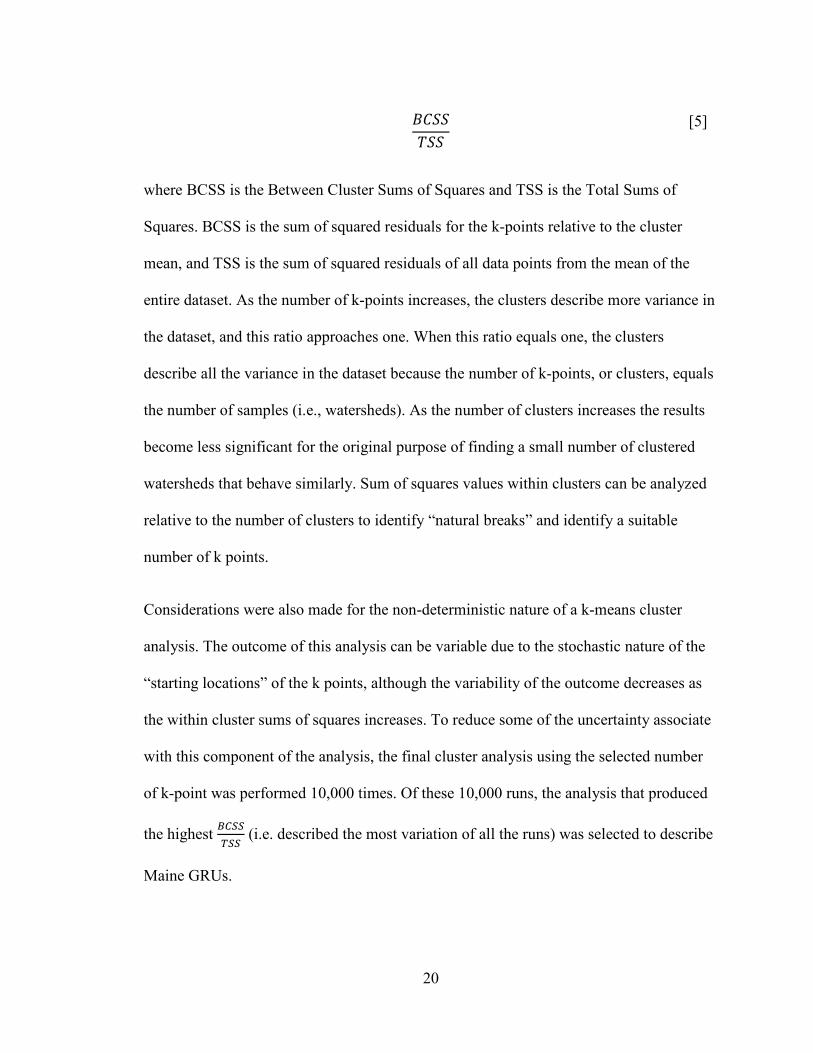
Equation 5: Percent of data variability described by clustering.
𝐵𝐵𝑃𝑃𝑄𝑄𝑄𝑄𝑇𝑇𝑄𝑄𝑄𝑄
xiv
Equation 6: Water balance equation.
𝑑𝑑𝑑𝑑𝑑𝑑𝑑𝑑
= 𝑃𝑃 − 𝐸𝐸𝑇𝑇 − 𝑄𝑄
Equation 7: Discharge as a function of storage.
𝑄𝑄 = 𝑓𝑓(𝑑𝑑)
Equation 8: Change in discharge over time as a function of system storage and water
budget parameters.
𝑑𝑑𝑑𝑑𝑑𝑑𝑑𝑑
= 𝑑𝑑𝑑𝑑𝑑𝑑𝑑𝑑
𝑑𝑑𝑑𝑑𝑑𝑑𝑑𝑑
= 𝑑𝑑𝑑𝑑𝑑𝑑𝑑𝑑
(𝑃𝑃 − 𝐸𝐸𝑇𝑇 − 𝑄𝑄)
Equation 9: Equation for the hydrograph sensitivity function.
𝑘𝑘 = 𝑑𝑑𝑑𝑑𝑑𝑑𝑑𝑑
= 𝑑𝑑𝑑𝑑𝑑𝑑𝑑𝑑𝑑𝑑𝑑𝑑𝑑𝑑𝑑𝑑
= 𝑑𝑑𝑑𝑑𝑑𝑑𝑑𝑑
𝑃𝑃−𝐸𝐸𝐸𝐸−𝑑𝑑=
−𝑑𝑑𝑑𝑑𝑑𝑑𝑑𝑑𝑑𝑑�𝑃𝑃≪𝑑𝑑,𝐸𝐸𝐸𝐸≪𝑑𝑑
Chapter Three:
Equation 10: Equation for the Nash-Sutcliffe Efficiency criteria (Nash and Sutcliffe
1970).
𝑁𝑁𝑄𝑄𝐸𝐸 = 1 −∑ (𝑂𝑂𝑑𝑑 − 𝐸𝐸𝑑𝑑)2𝑛𝑛𝑑𝑑=1
∑ (𝑂𝑂𝑑𝑑 − 𝑂𝑂�)2𝑛𝑛𝑑𝑑=1
Equation 11: Equation for percent bias.
𝑃𝑃𝐵𝐵𝑃𝑃𝐷𝐷𝑄𝑄 = ∑ (𝑂𝑂𝑑𝑑−𝐸𝐸𝑑𝑑)∗100𝑛𝑛𝑑𝑑=1
∑ (𝑂𝑂𝑑𝑑)𝑛𝑛𝑑𝑑=1
xv
Equation 12: Equation for root square residual.
𝑅𝑅𝑄𝑄𝑅𝑅 = 𝑅𝑅𝑅𝑅𝑅𝑅𝐸𝐸𝑅𝑅𝐸𝐸𝑆𝑆𝐸𝐸𝑆𝑆𝑜𝑜𝑜𝑜𝑜𝑜
= �∑ (𝑂𝑂𝑑𝑑−𝐸𝐸𝑑𝑑)2𝑛𝑛
𝑑𝑑=1
�∑ (𝑂𝑂𝑑𝑑−𝑂𝑂�)2𝑛𝑛𝑑𝑑=1
Equation B.1: Equation solving for the overland flow discharge per unit area along a cell
boundary in the x direction.
𝑣𝑣𝑥𝑥ℎ = 𝐾𝐾𝑥𝑥(−𝜕𝜕𝜕𝜕𝜕𝜕𝜕𝜕
)12ℎ
53
Equation B.2: Equation solving for the overland flow discharge per unit area along a cell
boundary in the y direction.
𝑣𝑣𝑦𝑦ℎ = 𝐾𝐾𝑦𝑦(−𝜕𝜕𝜕𝜕𝜕𝜕𝜕𝜕
)12ℎ
53
Equation B.3: Equation for total evapotranspiration using the two-layer water balance
method.
𝐸𝐸𝑇𝑇 = 𝐸𝐸𝑇𝑇𝑐𝑐𝑐𝑐𝑛𝑛 + 𝐸𝐸𝑇𝑇𝑝𝑝𝑝𝑝𝑛𝑛 + 𝐸𝐸𝑇𝑇𝑢𝑢𝑢𝑢 + 𝐸𝐸𝑇𝑇𝑠𝑠𝑢𝑢 + 𝐸𝐸𝑇𝑇𝑠𝑠𝑛𝑛𝑝𝑝𝑠𝑠
Equation B.4: Equation for determining infiltration using the two-layer water balance
method.
𝑃𝑃 = 𝑚𝑚𝑚𝑚𝑚𝑚 (𝑃𝑃𝑏𝑏 ,𝐾𝐾𝑠𝑠 ∗ ∆𝑑𝑑, (𝑉𝑉𝑠𝑠 − 𝜃𝜃) ∗ (𝜕𝜕 − ℎ)
Equation B.5: Linear reservoir method equation for the storage of a reservoir.
𝑑𝑑 = 𝑘𝑘 ∗ 𝑄𝑄
xvi
Equation B.6: The vertically integrated equation of the conservation of mass.
𝜕𝜕𝑄𝑄𝜕𝜕𝜕𝜕
+𝜕𝜕𝐷𝐷𝜕𝜕𝑑𝑑
= 𝑞𝑞
Equation B.7: The vertically integrated equation of the conservation of momentum.
𝜕𝜕𝑄𝑄𝜕𝜕𝑑𝑑
+𝜕𝜕(∝ 𝑄𝑄2
𝐷𝐷 )𝜕𝜕𝜕𝜕
+ 𝑔𝑔𝐷𝐷𝜕𝜕ℎ𝜕𝜕𝜕𝜕
+𝑔𝑔𝑄𝑄|𝑄𝑄|𝑃𝑃2𝐷𝐷𝑅𝑅
= 0
Equation B.8: Equation for temperature melting of snow.
𝑀𝑀𝐸𝐸 = 𝐽𝐽𝐸𝐸(𝑇𝑇 − 𝑇𝑇0)
Equation B.9: Equation for radiation melting of snow.
𝑀𝑀𝑅𝑅 = −𝐽𝐽𝑅𝑅𝑐𝑐𝑑𝑑𝑅𝑅𝑠𝑠𝑠𝑠
Equation B.10: Equation for energy melting of snow.
𝑀𝑀𝐸𝐸 = 𝐽𝐽𝐸𝐸𝑃𝑃(𝑇𝑇 − 𝑇𝑇0)
Chapter Four:
Equation 13: Sediment transport proportionality proposed by Henderson (1989).
𝑞𝑞𝑠𝑠𝐷𝐷32 ∝ (𝑞𝑞𝑄𝑄)2

xvii
Equation 14: A rearrangement of Equation 13 solving for the change in channel slope
over time.
𝑅𝑅1𝑅𝑅2
= (𝑞𝑞𝑜𝑜2𝑞𝑞𝑜𝑜1
)12(𝑞𝑞1𝑞𝑞2
)(𝑆𝑆2𝑆𝑆1
)34
Equation 15: Hydraulic geometry expression for channel width.
𝑤𝑤 = 𝑎𝑎𝑄𝑄𝑏𝑏
Equation 16: Hydraulic geometry expression for channel depth.
𝑑𝑑 = 𝑐𝑐𝑄𝑄𝑓𝑓
Equation 17: Hydraulic geometry expression for cross section averaged channel velocity.
𝑣𝑣 = 𝑘𝑘𝑄𝑄𝑚𝑚
Equation 18: Modified at-a-station hydraulic geometry relation.
𝑤𝑤𝑑𝑑
= 𝑗𝑗(𝐷𝐷𝐷𝐷)𝑟𝑟
Equation 19: Surface based sediment transport equation presented by Wilcock and Crowe
(2003).
𝑑𝑑𝑖𝑖 =𝜏𝜏𝑔𝑔𝜏𝜏𝑟𝑟𝑠𝑠𝑔𝑔
(𝐷𝐷𝑠𝑠𝑔𝑔𝐷𝐷𝑖𝑖
)𝑋𝑋
xviii
LIST OF ABBREVIATIONS AND NOTATIONS
∝ Momentum distribution coefficient
a, c, j Denotes variable coefficients
b, f, m, r Denotes variable exponents
A Cross sectional area
BCSS Between Cluster Sums of Squares
C Chezy’s resistance coefficient
Conc. Constituent concentration
CCSM Community Climate Systems Model
D Grain size
d Channel depth
DA Drainage Area
Et Expected (Modelled) discharge at time t
NSE Nash-Sutcliffe Efficiency criteria
EPA Environmental Protection Agency
EPSCoR Established Program to Stimulate Competitive Research
ET Evapotranspiration
ETcan Evapotranspiration from the vegetation canopy
ETpon Evapotranspiration from ponds and other sources of surface water storage
ETsnow Evapotranspiration from snow
ETsz Evapotranspiration from the saturated zone
ETuz Evapotranspiration from the unsaturated zone
g Acceleration due to gravity
GIS Geographic Information System
GRU Geomorphic Response Unit
h Hydraulic head
I Infiltration
IPCC Intergovernmental Panel on Climate Change
JT Degree-day factor for snow melt
JRad Radiation melting factor for snow melt
JE Energy snow melting coefficient for the energy of liquid rain
K Hydraulic conductivity
k Sensitivity Parameter (Chp. 2), variable coefficient (Chp. 4)
Ks Saturated hydraulic conductivity
l Variable loading
LAI Leaf Area Index
LGM Last Glacial Maximum
LULC Land Use/ Land Cover
xix
MT Temperature snow melting
MR Radiation snow melting
ME Energy snow melting
MeSSI Maine’s Sustainability Solutions Initiative
µ Fluid viscosity
n Manning’s roughness coefficient
nD The partitioned Manning’s roughness coefficient for sediment
NOAA National Oceanographic and Atmospheric Administration
O� Observed average discharge
Ot Observed discharge at time t
P Precipitation
Pb Surface ponding
PC Principal Component
PBIAS Percent Bias
Q Discharge
Qs Sediment transport rate
QLoad Mass flux of constituent
q Discharge per unit width
qs Sediment transport rate per unit width
qs∗ Dimensionless sediment transport rate
R Hydraulic radius
Rsw Incoming solar radiation
RD Rooting Depth
ρf Density (fluid)
ρs Density (sediment)
RMSE Root Mean Square Error
S Slope
s Relative grain density (ρs ρf� )
STDEV Standard Deviation
T Temperature
T0 Freezing temperature of snow
t Time
θ Soil water content
TSS Total Sums of Squares
τ Shear stress
τ∗ Dimensionless shear stress
τc Critical shear stress
τc∗ Dimensionless critical shear stress
τci Critical shear stress for sediment of size i
τg Partitioned shear stress acting on sediment, or grain shear stress
U Reach segment averaged velocity
Vs Volume of water at saturation
v Velocity

xx
W Water storage
w Channel width
X Denotes a variable
x, y, z Denotes cartesian coordinates
WCSS Within Cluster Sums of Squares
1
CHAPTER ONE
INTRODUCTION
1.1 Research Questions
The rates and magnitudes of watershed hydrologic processes in Northern New England
are dominantly influenced by climate, the post-glacial terrain, and landscape
modifications by humans following European colonization of the area in the early 1600’s
(Maine Historical Society 2014). The influence that human activities, climatic conditions,
and past glaciation exert on surface hydrology and fluvial geomorphology in the region is
the focus of this research. This dissertation summarizes analyses that identify and
quantify watershed geomorphology, climate conditions, surface flow regimes, and stream
channel dynamics. The study area extends through Central and Coastal Maine where
local economies and cultural identities have close ties to surface water resources and
water quality conditions affecting rivers, lakes, and coastal estuaries.
The core components of this dissertation were developed with input and collaborative
interactions with local stakeholder communities to define research objectives relevant to
water resource sustainability in the region. Three research questions framed around
processes governing water resource conditions in the study region are pursued using a
combination of field measurements, spatial data analysis, and numerical watershed
modeling. These research questions provide the organizational structure for the
dissertation:
2
1. How do watershed geomorphic conditions vary (e.g. geology, soils, relief, and
land cover) and how do the dissimilarities relate to stream flow
characteristics?
2. What are the implications of climate change to the surface flow regimes of
headwater stream systems in the region?
3. How do watershed conditions and flow regime alterations from climate
change affect stream channel dynamics?
Observations and research results are summarized throughout this document to address
the watershed management and sustainability challenges described by local communities,
environmental organizations, and government agencies charged with managing
environmental conditions and natural resources in Maine.
1.2 The Sediment-Water Proportionality
The research questions inspiring this project are related to watershed management and
fundamentally framed around relations between the availability of mobile sediment and
the capacity of surface flows to transport this sediment supply through and from
headwater streams (Wilcock et al. 2009). The fundamental proportionality between water
and sediment is an important consideration linked to management of nonpoint source
pollution, aquatic habitat, and drinking water supplies, particularly as it relates to
watershed and stream conditions, surface water discharge, and climate. The relation
between water discharge, sediment supply, and sediment transport provides an underlying
3
basis because of the direct associations with watershed alterations, human activities,
climate changes, and stakeholder water resource interests and concerns.
The transport of sediment in the modern Maine landscape is driven by surface water
discharge (Q), which is a function of watershed drainage area (DA):
𝑄𝑄 = 𝑓𝑓(𝐷𝐷𝐷𝐷) [1]
The rate at which sediment is transported (per unit width of stream) is a function of flow
strength (𝜏𝜏, i.e. shear stress), depth (ℎ), sediment grain size (𝐷𝐷), the density of the
sediment (𝜌𝜌𝑠𝑠) and water (ρ), fluid viscosity (𝜇𝜇), and gravity (𝑔𝑔):
𝑞𝑞𝑠𝑠 = 𝑓𝑓(𝜏𝜏,ℎ,𝐷𝐷,𝜌𝜌𝑠𝑠, 𝜌𝜌, 𝜇𝜇,𝑔𝑔) [2]
Stream channel dynamics are governed by the relation between components of equation
2, with channel cross section area and bottom substrate conditions responding to
alterations in water and sediment supplies. This proportionality between sediment and
water is conventionally framed by the Lane/Borland Balance in figure 1 (Borland 1960)
and the sediment-water proportionality:
𝑄𝑄𝑠𝑠𝐷𝐷 ~ 𝑄𝑄𝑄𝑄 [3]
where 𝑄𝑄𝑠𝑠 is the sediment transport rate and S is the channel slope. Changes to terms on
either side of the proportionality function produce a change in channel conditions.

4
Figure 1:The Lane/Borland channel stability relation. Adapted from Lane (1955).
The sediment-water proportionality in Maine’s deglaciated landscape presents a
condition of relatively low watershed sediment supply compared to locations south of the
limit of glaciation (USDA 2009). Sediment inputs from upland areas to streams are low
with the exception of locations where glacial features such as eskers and moraines are
present and in close proximity to waterways (Snyder et al. 2009). The historic glacial
activity in this landscape “reset” the geomorphology ~15 Kya as the Laurentide Ice Sheet
retreated from the region (Borns Jr. et al. 2004). The relatively thin veneer of young soils
and regolith present over bedrock today is an artifact of mechanical work by the
overburden of ice during glaciation and outwash during retreat. The glacial history
produced a limited modern supply of sediment, particularly grain sizes smaller than sand,
in large areas of the state with the exception of coastal areas that have fine-grained
5
sediments on the surface deposited during the transgression of the Atlantic Ocean prior to
isostatic rebound of the region.
The right-hand side of the sediment-water proportionality (Equation 3), transport
capacity, is influenced by all components of watershed hydrologic systems, including
types of precipitation, timing and rates of runoff production, and pathways of routing
through drainage networks. Although Maine has an average annual precipitation depth
(114 cm, NOAA 2007) similar to the Mid-Atlantic, the monthly hydrologic budget is very
different due to climate effects on snowfall and snowpack, vegetation, and
evapotranspiration. Surface routing pathways conveying excess precipitation as runoff
are also substantially modified by a multitude of lakes, ponds, and wetlands that were
created from glacial ice sheet dynamics. These reservoir features store surface water and
regulate the downstream movement of both water and sediment. Northern New England
is forecast to become increasingly wetter due to climate changes (Fernandez et al. 2015).
The effects of the hydrologic changes in the region on sediment transport competence and
capacity in headwater stream channels have not been quantified in most of the settings in
the region. The implications to stakeholder interests related to water resources and
aquatic habitat are therefore poorly understood, limiting the development of responsive
watershed management strategies for sustainability solutions.
1.3 Background: Sustainability Solutions Research in Maine
This research project grew out of two National Science Foundation (NSF) projects as part
of the Established Program to Stimulate Competitive Research (EPSCoR). The projects
focused on connecting knowledge with action, bridging the gap between academic
6
research and sustainability solutions through stakeholder-driven and scientifically
defensible management strategies. The project initially began in 2013 as part of research
activities included in the project portfolio of Maine’s Sustainability Solutions Initiative
(MeSSI) (National Science Foundation award EPS-0904155). A component of the MeSSI
project focused on the Sebago Lake watershed in southern Maine, inspired by concerns
around the vulnerability of the lake to future watershed modifications from land
development. This project sought to develop decision support tools for water resource
sustainability in this and other Northern New England lake systems. Much of the
landscape in the Sebago Lake watershed is dominated by private forestland, but socio-
economic projections have indicated increased land cover alterations in the region.
Projected regional population growth and the transition of the landscape to include more
suburban development over the next thirty years (U.S. EPA 2009) may have adverse
impacts on downstream water quality. These pressures and the use of Sebago Lake as a
drinking water resource for much of southern Maine’s population has made the watershed
one of the most at risk in the northeastern United States (Barnes 2009).
The geographic scale of the sustainability-focused research was expanded in 2015 as part
of the New England Sustainability Consortium (NEST) (National Science Foundation
award IIA-1330691). This project was centered on strengthening the link between science
and decision making, primarily as related to rules for beach closures to shellfish
harvesting areas in response to pollution problems. Many coastal Maine community
economies are linked to tourism, aquaculture, industrial fishing, and shellfish harvesting
industries that are dependent on good water quality in nontidal streams and rivers, tidal
estuaries, and coastal beach areas. Community culture and wellbeing are in many ways
7
connected to near and offshore water quality. Degradation in water quality has begun to
threaten these communities as the population along Maine’s coastline increases and the
effects from climate change become more prevalent (Evans et al. 2016; Taylor 2018;
Fernandez et al. 2015). Quantification of land-sea connections was at the heart of the
NEST research effort, with the goal of comparing the vulnerability of varied coastal
Maine landscape settings to water pollution problems.
The research summarized in this dissertation is an extension of these two projects focused
on sustainability solutions to water resource and aquatic habitat problems, examining
coupled social-biophysical systems in the Central and Coastal Maine region. The earth
science questions examined were inspired by stakeholder engagement, primarily state and
regional resource management agencies (e.g., Maine Department of Marine Resources
and the Portland Water District) during the MeSSI and NEST projects. This research
seeks to address research gaps related to management that are directly related to
sustainability solution goals. The research uses information gathered from previous
research and monitoring activities, knowledge of stakeholders, and data collected during
these projects to advance analyses of watersheds draining Maine’s landscape to support
management needs linked to water resources. The MeSSI and NEST project activities
included deployment and operation of a stream monitoring network. The NEST project
also synthesized new coastal Maine watershed delineations derived from high resolution
topographic (LiDAR) datasets that have only recently become available for the coastal
Maine region.

8
1.4 Study Region
The region of focus for this dissertation is Central and Coastal Maine. For the purposes of
this dissertation, the extent of Central and Coastal Maine will be broadly defined by the
White Mountains and the Piscataqua River to the south, the “Maine Highlands” to the
west, the Maine coastline to the east, and the Saint Croix River to the north/northeast
(Figure 2). The study region spans a range of elevations and geologic conditions. The
areas of highest relief and elevation are found along the Appalachian Range to the west,
and the landscape generally loses elevation and relief moving eastward. An exception to
this general trend is the coastline of Mid-Coast Maine where the expression of the
Acadian Orogeny produces some of the highest relief in the state. The entire region is
predominantly underlain by schistose bedrock with increasing metamorphism from south
to north (Osberg et al. 1985). However, several granitic plutons are present, most notably
throughout the high relief regions around the Mid-Coast and the Sebago Pluton that
underlies Sebago Lake and much of its contributing rim watershed.
A well-documented geomorphic boundary approximating the separation of Maine’s
Central and Coastal sub-regions is the demarcation of the extent of marine transgression
following the retreat of the Laurentide Ice Sheet (Woodrow and Borns 1985). West of the
marine transgression the surficial geology is mostly dominated by till with a scattered
mix of wetland, glacio-fluvial, and glacio-marine deposits. East of the marine
transgression the surface is largely dominated by fine grained marine deposits, although
the deposit thickness is relatively small or absent in portions of the Mid-Coast and
Downeast areas.

9
Figure 2: Study region site map.
10
Climatically, the coastal regions experience some moderating effects from the Gulf of
Maine relative to the central regions of the state. However, these difference between
regions is minimal. Averaged between 1895 and 2007, yearly temperature in the Central
and Coastal Maine region was ~6 °C and the region received approximately 114 cm of
precipitation (NOAA 2007). This precipitation falls as snow in winter months, producing
median seasonal snowpack depths between 500 and 800 mm (Cember and Wilks 1993).
The melting of this snow often results in large runoff events and seasonally high spring
stream flows (Dudley and Hodgkins 2002; Dudley and Hodgkins 2005).
Phase three of the Coupled Model Intercomparison Project (CMIP3) indicates an increase
in regional temperatures of around 6-7 °C over the next 100 years, with the largest
increase occurring during winter months (Jacobson et al. 2009). Over this same period,
precipitation is expected to increase. These simulations indicate an increase in winter
precipitation of approximately 8-14%, a 9-10% increase in spring precipitation, and an
increase of about 6% in the fall. Summer precipitation is forecasted to experience
minimal change.
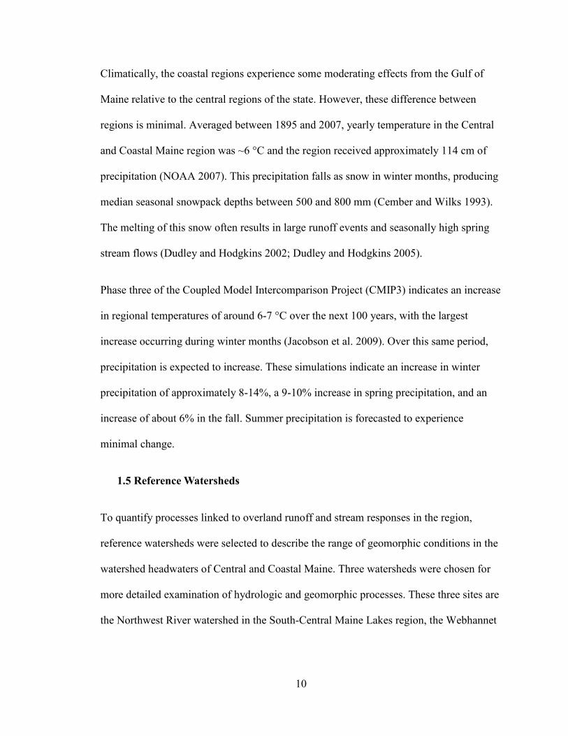
1.5 Reference Watersheds
To quantify processes linked to overland runoff and stream responses in the region,
reference watersheds were selected to describe the range of geomorphic conditions in the
watershed headwaters of Central and Coastal Maine. Three watersheds were chosen for
more detailed examination of hydrologic and geomorphic processes. These three sites are
the Northwest River watershed in the South-Central Maine Lakes region, the Webhannet
11
River watershed along the Southern Coast, and the Cromwell Brook watershed in Mid-
Coast Maine.
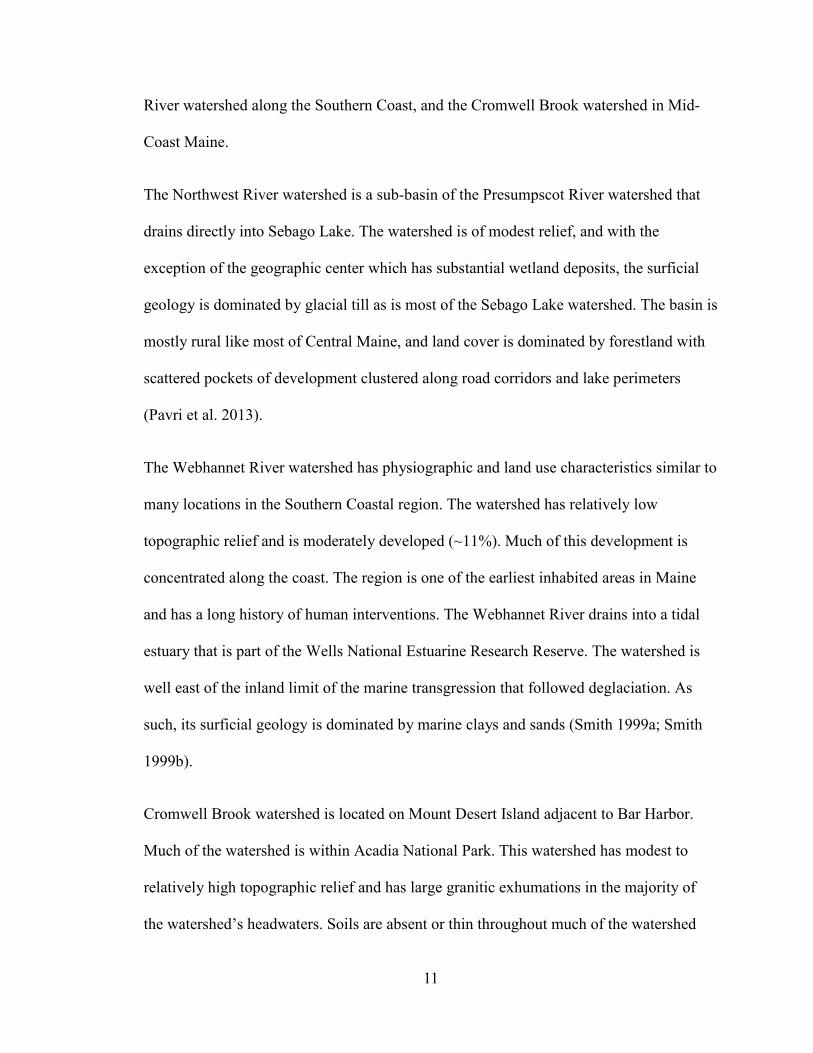
The Northwest River watershed is a sub-basin of the Presumpscot River watershed that
drains directly into Sebago Lake. The watershed is of modest relief, and with the
exception of the geographic center which has substantial wetland deposits, the surficial
geology is dominated by glacial till as is most of the Sebago Lake watershed. The basin is
mostly rural like most of Central Maine, and land cover is dominated by forestland with
scattered pockets of development clustered along road corridors and lake perimeters
(Pavri et al. 2013).
The Webhannet River watershed has physiographic and land use characteristics similar to
many locations in the Southern Coastal region. The watershed has relatively low
topographic relief and is moderately developed (~11%). Much of this development is
concentrated along the coast. The region is one of the earliest inhabited areas in Maine
and has a long history of human interventions. The Webhannet River drains into a tidal
estuary that is part of the Wells National Estuarine Research Reserve. The watershed is
well east of the inland limit of the marine transgression that followed deglaciation. As
such, its surficial geology is dominated by marine clays and sands (Smith 1999a; Smith
1999b).
Cromwell Brook watershed is located on Mount Desert Island adjacent to Bar Harbor.
Much of the watershed is within Acadia National Park. This watershed has modest to
relatively high topographic relief and has large granitic exhumations in the majority of
the watershed’s headwaters. Soils are absent or thin throughout much of the watershed

12
except for areas within the lowland valleys where the lowermost reaches of the waterway
traverse a landscape mostly covered by fined grained marine deposits, including clay
layers (NRCS 2016). The watershed is moderately developed, approximately 19%, much
of which is within Bar Harbor at the downstream end of the watershed.
1.6 Research Summary
This dissertation examines watershed dynamics across a range of spatial and temporal
scales within the study region. Primary data was collected between 2013 and 2017. In a
general order of succession, data were collected from the Sebago Lake, the Webhannet
River, and the Cromwell Brook watersheds. The structure of data collection and analysis
activities matches the progression of the project as described in Section 1.3. The
following chapters address the three research questions outlined above using a
combination of first-person observations, statistical techniques, and numerical modeling.
13
CHAPTER TWO
HEADWATER DRAINAGE AREA SETTINGS IN MAINE
2.1 Chapter Abstract
Watershed hydrology across Northern New England is responsive to the region’s history
of glaciation and human activities. Knowledge of surface flow characteristics and the
extent to which geomorphic features in a landscape influence watershed hydrology is
important for the development of sustainable water resource management strategies
across the region. This research evaluates landscape conditions relative to surface flow
characteristics in Maine to provide a basis for examining the transferability of water
resource management strategies in the state’s varied physiographic settings. A high
density of watershed measurements is ideal for adaptive management, but the capacity
for data collection is limited. A solution to the problem presented by the limited capacity
for continuous monitoring of surface water conditions in all places is to prescribe
management strategies relative to watershed settings defined by landscape conditions
affecting surface water hydrology and stream channel dynamics. The approach focuses
on landscape attributes governing the generation of excess precipitation and the routing
of runoff through watershed drainage networks. While not every relevant characteristic
driving watershed hydrology is captured at high resolution, watershed attributes most
prominently affecting surface water flow regimes and fluvial processes in headwater
stream drainage networks are considered. The watershed scale of evaluation is
conceptually similar to the “statistical and essential realism” examples of landscape

14
modeling presented by Dietrich et al. (2003), placing focus on prominent characteristics
that relate to contemporary earth surface processes.
Geomorphic characteristics of Maine’s landscape are examined, and dominant attributes
are grouped at the grain scale of moderately sized (third order) watersheds to describe
and compare landscape conditions with a focus on hydrologic variability in headwater
stream systems. The approach considers a range of time scales and processes affecting
contemporary landscape conditions, ranging from modern hydrology and surface erosion,
to deposits formed during deglaciation ~15 Kya, to continental scale processes shaping
the terrain millions of years ago.
Watershed conditions influencing surface water flows and stream dynamics in Maine are
grouped into nine statistically definable clusters referred to as Geomorphic Response
Units (GRUs) using geospatial data analysis. The clusters are assembled from a set of
attributes that govern headwater stream flows and morpho-dynamics. Analysis of flow
time series from USGS river gauging stations across the region are used to compare
hydrograph characteristics across GRUs. The comparisons provide a basis to quantify
surface hydrology and correlate them with geomorphic settings defined by the GRUs.
These analyses identify watershed “types” based on the collection of attributes and
establish a framework to evaluate the responses and vulnerabilities of varied watershed
settings to land use and climate changes in the region.
15
2.2 Introduction
The retreat of the Laurentide Ice Sheet ~15 Kya from the Northern New England region
exposed a landscape sculpted and carved by glacial process (Borns Jr. et al. 2004). The
landscape’s generally thin soils, till dominated surficial geology, and numerous lakes
were produced from the advancement and retreat of the ice sheet. These conditions which
describe the fundamental properties of the regional sediment-water proportionality
(Equation 3), produced a drainage network with a relatively small sediment supply and a
large volume of surface water storage as compared to other parts of North America below
the southern extent of glaciation (Kelley et al. 2011; Smith and Wilcock 2015). While
sediment transport is small compared to non-glacial environments, variability from the
regional conditions of the sediment-water proportionality are present where high
sediment supply exist from glacial deposits (e.g. eskers) in close proximity to stream
channels (Snyder et al. 2009).
While extensive investigation of runoff, stream conditions, and nonpoint source pollution
have been conducted in other regions in the Eastern USA, glaciated regions of the
Northeastern USA have received less examination (Leopold et al. 1964). The modern
drainage network in this deglaciated landscape has not been described in terms of its
morphometry or process of development by mechanical erosion driven by ice and surface
water flows. Locations and alignments of large rivers in the region are known to
correspond to prominent geologic features; however, the influence of Maine’s glacial
history on the characteristics of upland drainage networks is not well understood. This
information gap exists despite the fact that headwater streams are the most extensive
components of watershed drainage networks and are important to the sustainability of
16
public water supplies and aquatic habitat in the region. More information is necessary to
identify and clarify the processes that influence tributary water flow regimes, as well as
the physical and chemical connections between the upland landscape and downstream
rivers, lakes, and estuaries. The information gap related to headwater drainage networks
limits the ability for natural resource managers and environmental regulators to develop
strategies to respond to water quality, aquatic habitat, and safety problems linked to
watershed land use and climate changes.
This research provides a foundation to address this knowledge gap by focusing on
headwater watershed conditions that govern surface water hydrology, quantifying
watershed variability and relating identified watershed types to surface flow regime
characteristics. Clustering of headwater basins based on landscape characteristics provide
a means to identify settings more vulnerable to land use and climate changes and develop
decision tools for adaptive watershed management strategies.
Delineations of physiographic regions have been previously completed at various scales
to include the continental United States and Maine (Fenneman 1938; Toppan 1935).
Researchers in other regions of the United States have used similar approaches to guide
hydro-chemical sampling, interpretation of water quality information, and classify
hydrologic flow regimes for public policy claims (Preston 2001; Lipscomb 1998). Within
the study region, previous work has been performed to identify both biophysical and
climatic regions for natural resource management purposes (Briggs and Cornelius 1998;
Krohn, et al. 1999). This research expands these previous efforts, focusing on
geomorphic variables influencing surface water flows, stream channel conditions, and
related to water resource sustainability concerns.

17
2.3 Methods
2.3.1 Watershed Characterization
Data Collection: 8,274 drainage divides are delineated within the State of Maine by the
Maine Geologic Survey. These basins are sub-units of HUC-12 watersheds that have
been delineated based on USGS 1:24,000 scale topographic maps, averaging ~ 10 km2 in
size. Geospatial data for each watershed were assembled from GIS Databases available
through the Maine Office of GIS (http://www.maine.gov/megis/) and the USDA
(https://datagateway.nrcs.usda.gov/). Variables considered in the analysis were selected
based on their relevance to watershed hydrology, geomorphic watershed properties, and
data availability (Table 1).
Table 1: Variables used to characterize Maine’s landscape for PCA and cluster analysis. Variable Description Bedrock Geology
Percent of watershed underlain by Granoblastic, Metasedimentary, Chemical, Melange, Carbonate, Clastic, Volcanic, Plutonic, Magmatic, or Metaigneous bedrock.
Surficial Geology
Percent of watershed surficial geology that is Bedrock (Exposed), Gaciofluvial, Glaciomarine, Moraine, Till, Alluvium, Beach, Eolian, or Lake Bottom.
Land Cover/Use
Percent of watershed that is Developed, Agricultural Land, Forested, Storage, or Low Vegetation.
Hydrologic Soil Group
Percent of watershed that is classified as either A, B, C, or D soils by the State Soil Geographic database (STATSGO) (NRCS 2016).
Representative Slope
The estimated slope from STATSGO soil data.
Bedrock geology units, surficial geology units, and land cover types were grouped into
categories and the percent cover of each category was defined for the 8,274 watersheds.
Tables 8 and 9 in Appendix A summarize the categorization of surface geology and land
cover types. Information for bedrock geology classification and grouping is provided by

18
the USGS Mineral Resources On-Line Spatial Database, https://mrdata.usgs.gov.
Variable selection and categorization produced a dataset of 8,274 samples (watersheds)
by 34 variables.
Analysis: A Principle Component Analysis (PCA) was performed to find linear
combinations of variables that captured the maximum variation across Maine watersheds
(Harris 2001). The methodology of a PCA can be represented as:
𝑃𝑃𝑃𝑃1 = 𝑙𝑙1,1𝑋𝑋1 + 𝑙𝑙1,2𝑋𝑋2+…+𝑙𝑙1,𝑛𝑛𝑋𝑋𝑛𝑛=𝑿𝑿𝑿𝑿𝟏𝟏 𝑃𝑃𝑃𝑃2 = 𝑙𝑙2,1𝑋𝑋1 + 𝑙𝑙2,2𝑋𝑋2+…+𝑙𝑙2,𝑛𝑛𝑋𝑋𝑛𝑛=𝑿𝑿𝑿𝑿𝟐𝟐
: : : : : :
𝑃𝑃𝑃𝑃𝑛𝑛 = 𝑙𝑙𝑛𝑛,1𝑋𝑋1 + 𝑙𝑙𝑛𝑛,2𝑋𝑋2+…+𝑙𝑙𝑛𝑛,𝑛𝑛𝑋𝑋𝑛𝑛=𝑿𝑿𝑿𝑿𝒏𝒏
[4]
where PC is a principal component, X is a variable, and l is a loading or weight applied to
a variable as a coefficient when calculating the principal component. Weights are defined
for each variable in order to maximize the total variation while requiring that the squares
of the coefficients involved in any PC sum to one. As PCs are defined for as many
variables as are used in the analysis, each successive PC explains less variation in the
dataset.
In finding principal components which maximize variation, the analysis is sensitive to
differences of scale between variables. Variables with larger values are more likely to be
identified as principal components. For this reason, variables were translated to
normalized z-scores (each data point was transformed to represent the number of standard
deviations it appeared from the mean value of the variable). Following PCA analysis, the
Rule N-criterion was used to determine which principle components to retain (Lipscomb
1998; Preisendorfer et al. 1981). This technique compares the resulting PC eigenvalues,

19
which define the variance described by each principal component, to PC eigenvalues
derived from analysis of a random data matrix of equal dimensions (i.e. the 8,274
samples by 34 variables). Principal components are only retained if the ratio of 𝑃𝑃𝑃𝑃𝑎𝑎𝑎𝑎𝑑𝑑𝑎𝑎𝑎𝑎𝑎𝑎𝑃𝑃𝑃𝑃𝑟𝑟𝑎𝑎𝑛𝑛𝑑𝑑𝑜𝑜𝑟𝑟
exceeds one, that is, the PCs are only retained if they describe more variance in the actual
dataset than they would in a random dataset.
A k-means cluster analysis was performed to identify GRUs across the study region. A k-
means cluster analysis is an iterative multivariate technique used to identify natural
groupings in data by minimizing Within Cluster Sums of Squares (WCSS) relative to k
user specified points (Crawley 2012; Harris 2001; SAS Institute Inc. 1985; Sokal and
Rohlf 1995) (Figure 3). The principal components retained based on the Rule-N criterion,
and their scores, were used in the analysis to describe watershed characteristics in place
of the original variables.
Identification of the most suitable k user specified points often relies on a priori
knowledge of the dataset population and/or underlying causes that might drive natural
groupings within the data. The associated complexity of geomorphic data defining
watershed conditions causes ambiguity for determining the number of k points used in
this cluster analysis. Therefore, to identify the most suitable number of k points for
categorizing these watersheds, cluster analyses were run with a range of k points from
two to fifty. For each of these analyses the variation in the data explained by clustering
was analyzed (Equation 5):
20
𝐵𝐵𝑃𝑃𝑄𝑄𝑄𝑄𝑇𝑇𝑄𝑄𝑄𝑄
[5]
where BCSS is the Between Cluster Sums of Squares and TSS is the Total Sums of
Squares. BCSS is the sum of squared residuals for the k-points relative to the cluster
mean, and TSS is the sum of squared residuals of all data points from the mean of the
entire dataset. As the number of k-points increases, the clusters describe more variance in
the dataset, and this ratio approaches one. When this ratio equals one, the clusters
describe all the variance in the dataset because the number of k-points, or clusters, equals
the number of samples (i.e., watersheds). As the number of clusters increases the results
become less significant for the original purpose of finding a small number of clustered
watersheds that behave similarly. Sum of squares values within clusters can be analyzed
relative to the number of clusters to identify “natural breaks” and identify a suitable
number of k points.
Considerations were also made for the non-deterministic nature of a k-means cluster
analysis. The outcome of this analysis can be variable due to the stochastic nature of the
“starting locations” of the k points, although the variability of the outcome decreases as
the within cluster sums of squares increases. To reduce some of the uncertainty associate
with this component of the analysis, the final cluster analysis using the selected number
of k-point was performed 10,000 times. Of these 10,000 runs, the analysis that produced
the highest 𝐵𝐵𝑃𝑃𝑅𝑅𝑅𝑅𝐸𝐸𝑅𝑅𝑅𝑅
(i.e. described the most variation of all the runs) was selected to describe
Maine GRUs.

21
Figure 3: Example of the iterative procedure for a k-means cluster analysis in two dimensions, where k equals 3 user specified clusters. A through D are sequential representations of iterations.
22
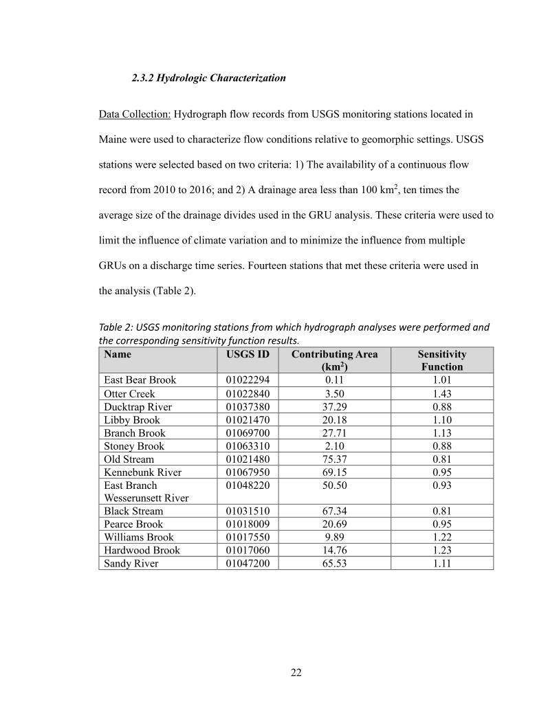
2.3.2 Hydrologic Characterization
Data Collection: Hydrograph flow records from USGS monitoring stations located in
Maine were used to characterize flow conditions relative to geomorphic settings. USGS
stations were selected based on two criteria: 1) The availability of a continuous flow
record from 2010 to 2016; and 2) A drainage area less than 100 km2, ten times the
average size of the drainage divides used in the GRU analysis. These criteria were used to
limit the influence of climate variation and to minimize the influence from multiple
GRUs on a discharge time series. Fourteen stations that met these criteria were used in
the analysis (Table 2).
Table 2: USGS monitoring stations from which hydrograph analyses were performed and the corresponding sensitivity function results. Name USGS ID Contributing Area
(km2) Sensitivity Function
East Bear Brook 01022294 0.11 1.01 Otter Creek 01022840 3.50 1.43 Ducktrap River 01037380 37.29 0.88 Libby Brook 01021470 20.18 1.10 Branch Brook 01069700 27.71 1.13 Stoney Brook 01063310 2.10 0.88 Old Stream 01021480 75.37 0.81 Kennebunk River 01067950 69.15 0.95 East Branch Wesserunsett River
01048220 50.50 0.93
Black Stream 01031510 67.34 0.81 Pearce Brook 01018009 20.69 0.95 Williams Brook 01017550 9.89 1.22 Hardwood Brook 01017060 14.76 1.23 Sandy River 01047200 65.53 1.11

23
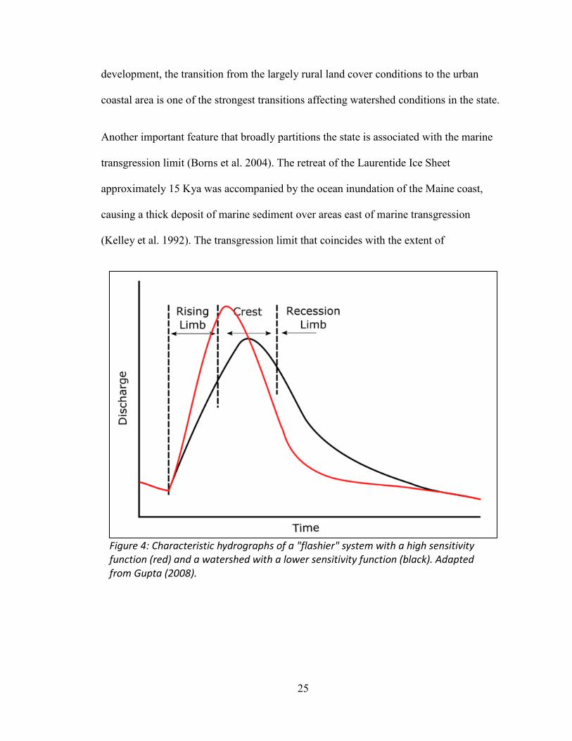
Analysis: Analysis focused on the sensitivity parameter, k, that describes the sensitivity
of discharge in a stream to changes in storage within a landscape (Kirchner 2009). A
large k indicates less storage and a smaller k indicates more storage. An example of this
is shown in Figure 4. The steeper recession limb associated with watershed A (red),
indicates that this watershed has less storage than watershed B (black).
The sensitivity parameter can be solved for by starting with a simple water balance:
𝑑𝑑𝑑𝑑𝑑𝑑𝑑𝑑
= 𝑃𝑃 − 𝐸𝐸𝑇𝑇 − 𝑄𝑄 [6]
where W is storage, t is time, P is precipitation, ET is evapotranspiration, and Q is
discharge. Using the linear reservoir theory, discharge can be defined as a function of
storage.
𝑄𝑄 = 𝑓𝑓(𝑑𝑑) [7]
Through differentiation and substitution, we can define discharge over time as:
𝑑𝑑𝑄𝑄𝑑𝑑𝑑𝑑
=𝑑𝑑𝑄𝑄𝑑𝑑𝑑𝑑
𝑑𝑑𝑑𝑑𝑑𝑑𝑑𝑑
=𝑑𝑑𝑄𝑄𝑑𝑑𝑑𝑑
(𝑃𝑃 − 𝐸𝐸𝑇𝑇 − 𝑄𝑄) [8]
The relation can then be rearranged to derive the sensitivity parameter using only the
discharge hydrograph when precipitation and evapotranspiration are relatively small.
That is, we can estimate the amount of storage in the watershed using only the
hydrograph.

24
𝑘𝑘 =
𝑑𝑑𝑄𝑄𝑑𝑑𝑑𝑑
= 𝑑𝑑𝑄𝑄𝑑𝑑𝑑𝑑𝑑𝑑𝑑𝑑𝑑𝑑𝑑𝑑
= 𝑑𝑑𝑄𝑄𝑑𝑑𝑑𝑑
𝑃𝑃 − 𝐸𝐸𝑇𝑇 − 𝑄𝑄= −𝑑𝑑𝑄𝑄𝑑𝑑𝑑𝑑𝑄𝑄
�
𝑃𝑃≪𝑑𝑑,𝐸𝐸𝐸𝐸≪𝑑𝑑
[9]
Periods of the hydrograph during which precipitation and evapotranspiration terms are
small were selected by this method. Conditions were assumed to be adequately met when
the slope of the hydrograph was negative, an assumption considered reasonable based on
the relatively small size of the watershed systems. Through trial and error, averaging the
data over a three-hour time step was found to best fit the measurement resolution of the
gauge data. Hydrograph slope and discharge at a three-hour time-step were calculated
and a power function was fit through the relation. The slope of the power function is the
sensitivity parameter describing the water storage properties.
2.4 Results and Discussion
2.4.1 Watershed Characterization
Rule-N criterion of the Principal Component Analysis resulted in the retainment of the
first ten principal components. Loadings for PC1, which describe the most variation, are
dominated by the contrast between developed and forested landscapes, glaciomarine and
till dominated surficial geologies, and well drained soils versus those which are more
moderate to poorly drained. These results conform with estimated outcomes based on
observations across this landscape. Maine is a predominantly rural state with isolated
developed zones along the southern coast near Portland, ME, the largest city in the state.
Unlike more populated parts of the U.S.A. that have extensively distributed urban
25
development, the transition from the largely rural land cover conditions to the urban
coastal area is one of the strongest transitions affecting watershed conditions in the state.
Another important feature that broadly partitions the state is associated with the marine
transgression limit (Borns et al. 2004). The retreat of the Laurentide Ice Sheet
approximately 15 Kya was accompanied by the ocean inundation of the Maine coast,
causing a thick deposit of marine sediment over areas east of marine transgression
(Kelley et al. 1992). The transgression limit that coincides with the extent of
Figure 4: Characteristic hydrographs of a "flashier" system with a high sensitivity function (red) and a watershed with a lower sensitivity function (black). Adapted from Gupta (2008).
26
widespread marine deposits runs perpendicular to the coast and partitions the state into
two distinct regions. In contrast to the coastal marine deposits, regions northwest of the
marine transgression limit are predominantly covered by glacial till deposits (Thompson
1985). These distinct surficial geologic conditions provide varied environments for the
development of soil conditions, producing extensive distributions of well drained soils in
the northwest regions of the state and more poorly drained soils in coastal areas.
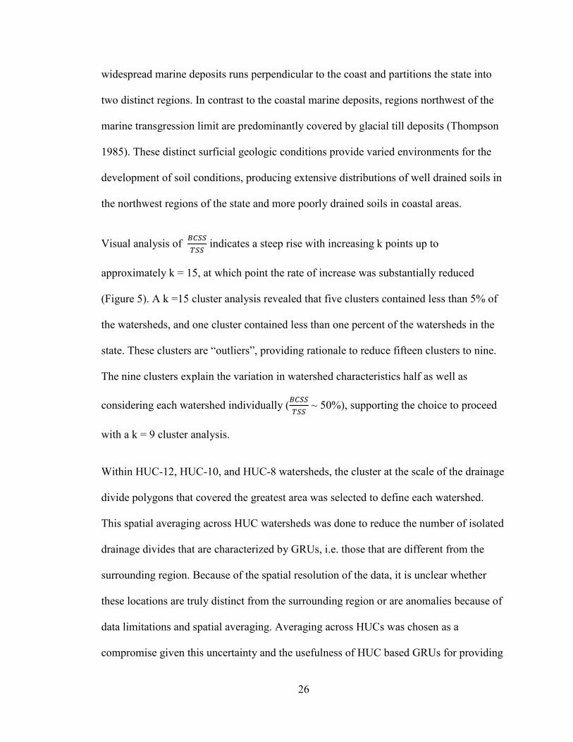
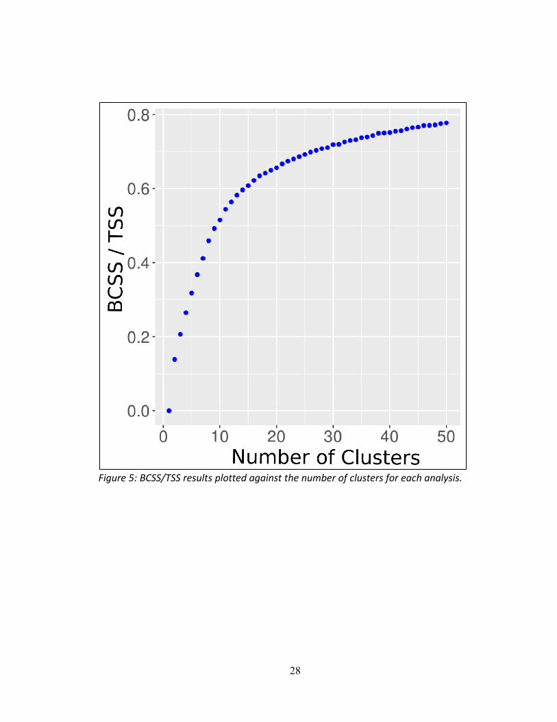
Visual analysis of 𝐵𝐵𝑃𝑃𝑅𝑅𝑅𝑅𝐸𝐸𝑅𝑅𝑅𝑅
indicates a steep rise with increasing k points up to
approximately k = 15, at which point the rate of increase was substantially reduced
(Figure 5). A k =15 cluster analysis revealed that five clusters contained less than 5% of
the watersheds, and one cluster contained less than one percent of the watersheds in the
state. These clusters are “outliers”, providing rationale to reduce fifteen clusters to nine.
The nine clusters explain the variation in watershed characteristics half as well as
considering each watershed individually (𝐵𝐵𝑃𝑃𝑅𝑅𝑅𝑅𝐸𝐸𝑅𝑅𝑅𝑅
~ 50%), supporting the choice to proceed
with a k = 9 cluster analysis.
Within HUC-12, HUC-10, and HUC-8 watersheds, the cluster at the scale of the drainage
divide polygons that covered the greatest area was selected to define each watershed.
This spatial averaging across HUC watersheds was done to reduce the number of isolated
drainage divides that are characterized by GRUs, i.e. those that are different from the
surrounding region. Because of the spatial resolution of the data, it is unclear whether
these locations are truly distinct from the surrounding region or are anomalies because of
data limitations and spatial averaging. Averaging across HUCs was chosen as a
compromise given this uncertainty and the usefulness of HUC based GRUs for providing

27
a more workable framework for watershed management applications. Based on visual
analysis and field observations, averaging drainage divide clusters into HUC-10 based
GRUs was found to be the most appropriate “grain scale” for identifying GRUs in the
state. Averaging into HUC-12 watersheds produced little change, and details from the
drainage basins were lost when averaging across the large HUC-8.
The nine defined GRUs across HUC-10 watersheds span a range of conditions that can be
broadly categorized by the dominant variables in each unit (Table 3).
Table 3: Attributes defining each Geomorphic Response Unit. Geomorphic
Response Unit Primary Location Dominant Attributes
GRU 1 Mid-Coast and Central Region Metasedimentary bedrock, C soils (poorly drained), and a
surficial till
GRU 2 Northern Maine Clastic bedrock and surficial till
GRU 3 Inland southern Maine A soils (well drained) and glaciofluvial deposits
GRU 4 Downeast Region Poorly drained soils
GRU 5 Kathadin Region C soils (poorly drained) and a moraines
GRU 6 Inland Downeast Region, Lakes
Region, and the Appalachian Mountains of Southern Maine
High relief, till, and plutonic bedrock
GRU 7 Mount Desert Island and surrounding area
High relief and exposed bedrock
GRU 8 St. John watershed in Northeastern Maine
B soils (moderately well drained), carbonate bedrock,
and agriculture
GRU 9 Southern Coast Urban development and glaciomarine clay
28
Figure 5: BCSS/TSS results plotted against the number of clusters for each analysis.
29
2.4.2 Hydrologic Characterization
Hydrograph analysis of the fourteen USGS gauge stations across Maine suggests a
quantifiable geospatial relation between flow characteristics and watershed settings
defined by GRUs. Monitoring stations along the coast that are within more poorly
drained, developed, and/or higher relief GRUs have higher sensitivity parameter values.
These geomorphic settings are more conducive to increased surface runoff, producing
flashier flow regimes. These flashier systems are more responsive to precipitation, with
quickly increasing flows as rain falls within the drainage area. This contrasts with
hydrographs analyzed throughout the central region that have lower sensitivity parameter
values. These monitoring stations are situated in GRUs with surficial geologies
dominated by till. Till throughout the region is generally well drained, resulting in higher
infiltration, less surface runoff, and more storage throughout the watershed system.
Transitioning further west, monitoring station hydrographs begin to have sensitivity
parameter values more consistent with those along the coast. These monitoring stations
have higher relief than the central locations and more agricultural land cover.
These results provide support for the defined GRUs through a quantifiable relation
between hydrographs and the watershed characteristics that govern the surface flow of
water through these systems. Within the limited extent of Maine, this analysis displays
the variability of current flow conditions due to a combination of historic and ongoing
landscape modification by humans and geologic processes, both glacial processes on the
order of ~15 Kya and endogenic processes on the order 50 to 350 Mya.

30
2.5 Conclusions
Results indicate that variation across Maine watersheds is most prominently represented
by the contrast between developed and forested landscapes, followed by the division
between the glaciomarine and the till dominated surficial geology. Watersheds with
extensive urban development in Maine’s mostly rural landscape are unique and the
dissimilarities impact the surface watershed hydrology. Landscape dynamics driven by
Maine’s glacial history also creates a notable geologic partition along the marine
transgression limit. The boundary coincides with a change in the dominant surface
materials with well drained till to the Northwest and poorly drained marine deposits
along the coast. The partition is the cause of substantial variation in watershed conditions
driving surface water flows in the state.
This analysis led to the division of HUC-10 watersheds across Maine’s post-glacial
landscape into nine statistically distinct GRUs with predictable variations in stream flow
conditions. The objective of this research was developed around regional stakeholder
concerns about water resource sustainability and vulnerabilities. The quantification and
classification of watershed conditions presented here through GRU development provides
a basis for stakeholder communities to customize regional watershed management
strategies in response to land use and climate changes affecting water quality, aquatic
habitat, and other ecosystem services provided by nontidal headwater streams. This
information also provides groundwork and an organizing framework for investigations of
surface runoff, nonpoint source pollution, and stream channel dynamics that can inform
adaptive strategies for water resource sustainability solutions in Maine.

31
2.6 Acknowledgements
The research described in this chapter was funded by the Maine Water Resources
Research Grants Program (Project Number: 5406025) and two National Science
Foundation EPSCoR projects: 1) Maine’s Sustainability Solutions Initiative (National
Science Foundation award EPS-0904155); and 2) New England Sustainability
Consortium (National Science Foundation award IIA-1330691). In addition to review
and input from committee members, I’d like to thank Kate Beard and Aaron Weiskittel
for help regarding clustering and PCA methodology. Thanks also to Lindsey White for
help coordinating and organizing the GIS data used in these analyses.

32
Figure 6: Sensitivity function values for Maine USGS watersheds plotted across GRUs.
33
CHAPTER THREE
THE HYDROLOGIC SIGNATURE OF NORTHEASTERN HEADWATER
BASINS
3.1 Chapter Abstract
This research uses watershed simulations to evaluate the impact of projected climate
modifications on hydrologic conditions in three Central and Coastal Maine watersheds,
quantifying surface flows in three dominant physiographic settings in the region. A series
of watershed hydrology scenarios were developed using climate information derived
from the Coupled Model Intercomparison Project (CMIP5) to examine the effects of
climate change on snow melt, watershed hydrology, and surface flow regimes within
settings represented by the study watersheds. Research objectives were defined through
engagement with regional stakeholders and identification of concerns related to water
resource sustainability in the region and capacity to respond to problems from forecasted
land use and climate changes. Results are framed to address these concerns and to
provide information relevant to water resource planning in the post-glacial Northeast
(USA) region.
Scenario simulation results indicate a substantial decrease in total snow water equivalent
across all watersheds and a shift in the seasonal termination of snow melt ranging from
ten to twenty days. The snowpack changes produce alterations in the timing and
magnitude of surface flows dominated by snow melt contributions in late winter and
early spring months. Surface flow rates during the remainder of the year are generally
predicted to increase except where low flows are dominantly regulated by outflows from
34
surface water storage locations in ponds or wetlands. Low (base) flows are predicted to
decrease slightly in locations with relatively high storage capacity due to increased
evapotranspiration rates in response to forecasted temperature increases. These modeling
outcomes present the range and variability of flow condition modifications the region
may experience over the next century. Results from this research provide a basis for
regionally and locally focused climate change adaptation strategies in varied post-glacial
settings defined by topography, surface geology, land cover, surface water storage, and
local climatic conditions.
3.2 Introduction
A river’s flow regime is described by patterns of discharge over time, including the
magnitude, frequency, duration, timing, and rate of flow change over annual periods of
record (Poff et al. 1997). These patterns are governed by the climate, biota, surface
geology, and landscape history that govern runoff production (e.g., infiltration rates) and
surface flow hydraulic conditions (e.g., hydraulic roughness and surface water storage in
ponds and wetlands). Alterations to these conditions produces flow regime modifications,
which directly impacts a system’s sediment-water proportionality. Increases or decreases
in the magnitude or frequency of moderate to high flows can alter sediment transport,
leading to channel adjustment and changes in the transport rate of constituents
downstream. These modifications present major challenges to water resource
sustainability because of the water budget implications to the water supply, the impact of
altered transport of constituents to water quality, and the effect of channel morphology
dynamics that affect aquatic habitat (Sparks 1995; Ward and Stanford 1995; Poff et al.
1997).

35
Humans commonly modify flow regimes through direct and indirect changes to drainage
patterns and watershed conditions (Poff et al. 1997). Direct modifications include channel
straightening, dredging, channelization, damming, and network expansion through the
connection of urban storm drain systems to the “natural” drainage system. Indirect
hydrologic modifications are produced by land use and cover (LULC) changes,
topographic modifications (Jones 2013), and the effects of climate change on stream
flows.
Knowledge of the associations between physiographic settings defined by climate and
watershed characteristics and surface flow regimes can provide a basis for forecasting the
effects of land use and climate changes on aquatic habitat and pollution related to
watershed runoff. This research defines these associations to address stakeholder
concerns related to instream habitat and downstream water quality. Stakeholders groups
engaged within the Lakes Region, Southern Coast, and Mid-Coast settings of Maine
(Toppan 1935) highlighted the strong tie between socio-economic conditions and the
sustainability of these resources. Increasing development pressure (U.S. EPA 2009)
within the predominantly rural and forested Lakes Region is a concern for downstream
water quality, particularly in the Sebago Lake watershed that provides municipal water
for 200,000 Maine residents (Portland Water District 2012). Within the Southern Coast
and Mid-Coast regions, both similar in the greater extent of urban development compared
to other parts of the state, the demand to address water resources sustainability is derived
primarily from tourism and seafood industries. These industries and local communities
are adversely affected by beach closures and water quality problems related to non-point
source pollution that result in shellfishing area closures. The demands on these water
36
resources and the uncertainty of non-point source pollution makes these systems high
priority locations for coupled climate-landscape-hydrology research in the New England
region.
This research supplements previous documentation of decadal time scale changes in
surface water resources in the region (Collins 2009). Building on this work, stakeholder
concerns are addressed using a distributed numerical watershed model to examine the
regional associations of climate, landscape, and watershed hydrology at the century time
scale. This approach has previously been utilized in a range of geographic conditions and
scales to examine the outcomes of multiple watershed processes and to evaluate a variety
of watershed conditions affecting surface water flows (Chu et al. 2013; Sahoo et al. 2006;
Wijesekara et al. 2012). The simulations of hydrologic processes governing surface flow
rates provides a basis to compare the effects of predicted climate change modifications to
aquatic habitat and water quality among dominant watershed settings in Maine.
3.3 Methods
3.3.1 Study Sites
Areas selected for evaluations were chosen based on geomorphic setting and watershed
size. Emphasis was focused on quantifying hydrologic conditions in three watersheds that
span a range of conditions but are comparable in size. All of the watersheds were modest
in size, reducing variability of physiographic and land use conditions, allowing
calibration with limited weather data, and requiring decreasing computational
requirements over the multiple calibration, validation, and scenario runs.

37
The Northwest River watershed was selected to represent landscape conditions in the
Lakes Region. The Northwest River is a sub-basin of the Sebago Lake watershed. This
watershed is the largest of the three study sites with a drainage area of 58 km2. Like much
of the Sebago Region, relief in the watershed is modest, and the bedrock is predominantly
associated with the Sebago pluton. The watershed’s surficial geology is dominated by till
deposits, although wetland deposits cover large areas in the center of the watershed
(Thompson et al. 1985). Characteristic of the region, numerous lakes and ponds are
present, producing a large storage signature in the hydrology and water budget. Land
cover throughout the watershed is predominantly rural with pockets of higher
development along the lake perimeter.
The Webhannet River watershed sits along the Southern Maine Coast, covering 27 km2
of mostly low relief terrain. The area is moderately developed (~11%), much of which is
concentrated along the coast, and has a long history of human interventions. The surficial
geology of the watershed is predominantly composed of marine clays and sands (Smith
1999a; Smith 1999b) corresponding to its location east of the line of marine
transgression.
The Cromwell Brook watershed is in Mid-Coast Maine on Mount Desert Island, just
outside of Acadia National Park. The watershed is ~18 km2 and has moderate to high
relief. The location is dominated by the presence of shallow granites with thin or absent
soils. It is moderately developed (19%, mostly outside of Acadia National Park), and
much like the Webhannet River watershed this development is concentrated along the
coast.
38
Climatic conditions in the three watersheds are similar, although coastal areas are
affected by maritime climate conditions (Jacobson et al. 2009; Vose et al. 2014). Between
1895 and 2007 the central Maine region received an average of 114 cm of precipitation
annually and the average annual temperature was 6.19 °C (National Climate and Data
Center). The Coastal Region received slightly more precipitation during this period, 118
cm annually, and was slightly warmer, 6.83 °C. In the winter months most precipitation
falls as snow in all physiographic sub-settings. Southern regions experience earlier
seasonal melts and generally smaller total annual snow water equivalent. Snowpack
melting in the late winter and early spring month produces seasonally predictable and
sustained high flow conditions called the “freshet” (Hodgkins et al. 2003).
3.3.2 Model Parameterization and Calibration
The distributed watershed modeling platform, MIKE SHE, was parameterized for all
three watersheds using a combination of literature, spatial data, and field measurements
(Table 4). The computational approaches for various phases of the water cycle included
lumped and distributed approaches based on available data, data quality, and data
resolution. These approaches are standardized for all watershed simulations (Figure 9).
Domain resolutions were variable and based on the contributing areas for the basin
monitoring sites. The resolution of both the Cromwell Brook and Webhannet River
watershed models was 30m2 while the Northwest River model resolution was 50m2.
Models were calibrated using a multi-objective approach; The primary objective was the
matching of observed and modeled discharge, the secondary objective was the matching
of observed and modeled snow water equivalent, and the third objective was to evaluate
modeled water budget components relative to expected values.
39
Observed flow data in the Northwest River watershed was recorded by collaborators near
the confluence of the Northwest River and Sebago Lake (Reeve et al. 2013). A pressure
sensor was deployed to continuously measure water flow stage at 15-minute intervals that
was converted to a surface flow time series based on a rating curve assembled from
periodic manual discharge measurements (Rantz 1982a, 1982b). The rating curve derived
for the site was tested and verified by the deployment of an Acoustic Doppler Profiler
(Sontek-IQ) from mid-2015 to mid-2016. This instrumentation provided continuous
automatic discharge measurement comparison with recorded stage measurements from
the deployed pressure transducer. These methods produced nearly five years of flow data
from mid-2011 to early 2017.
Acoustic sensors (Teledyne ISCO, Submerged Probe Flow Module 720) were deployed
within the Cromwell Brook mainstem from mid-2015 through 2016. Construction
activities in Cromwell Brook in mid-summer 2016 disturbed the latter portion of the
dataset. Data was recorded at 10-minute intervals and coupled with periodic manual flow
measurements to develop rating curves, the same methodological approach that was
applied at the Northwest River.
The third study location, the Webhannet River watershed, was also monitored using
instrumentation deployed in the Webhannet River and a tributary, Depot Brook. Periodic
flow measurements were collected to construct rating curves. Hydraulic measurements
and time series data indicate that flows at these two locations can be correlated with a

40
Figure 7: Location map of watersheds respective of Maine GRUs.

41
Figure 8: Hydrologic signature for the Northwest River. This presents the characteristic flow regime structure for the river system over the ten-year period of “current conditions.”
nearby USGS gauge station (Kennebunk River, USGS 01067950) using standard
approaches for flow normalization by drainage area (Gupta 2008). This approach
produced continuous flow time series for the Webhannet River and Depot Brook from
2012 through 2016.
All watersheds and river monitoring sites were dominated by ice over conditions in
winter months. These conditions limited flow measurements for approximately three
months each year, resulting in less reliable flow data between December and March.
Observed flow datasets were omitted from the datasets during this time from all
monitoring stations for this reason.
42
Evaluation of model accuracy relied on multiple lines of evidence from a combination of
statistical measures to include the Nash-Suttcliffe Efficiency criteria (NSE), Percent Bias
(PBIAS), and the Root Mean Square Residual (RSR). NSE is a dimensionless,
normalized statistic that compares the residual variance of a simulation dataset relative to
the observed (measured) data variance (Moriasi et al. 2007; Nash and Sutcliffe 1970).
NSE values vary between negative infinity and one, with lower values indicating a poorer
fit, zero indicating a fit that would be achieved through assuming the average observed
value at each time step of the dataset, and a value of one indicating a perfect fit between
the model and observed data. NSE can be expressed as:
𝑁𝑁𝑄𝑄𝐸𝐸 = 1 −
∑ (𝑂𝑂𝑑𝑑 − 𝐸𝐸𝑑𝑑)2𝑛𝑛𝑑𝑑=1
∑ (𝑂𝑂𝑑𝑑 − 𝑂𝑂�)2𝑛𝑛𝑑𝑑=1
[10]
where 𝑂𝑂𝑑𝑑 and 𝐸𝐸𝑑𝑑 are the observed and predicted discharge at time t, respectively, and 𝑂𝑂� is
the average observed discharge.
PBIAS is an error index which measures the tendency of a model to over or underpredict
relative to the observed dataset (Gupta et al. 1999; Moriasi et al. 2007). A PBIAS of zero
indicates no bias in the modeled data set, while negative values indicate persistent over
prediction and positive values indicate underprediction. PBIAS is expressed as:
𝑃𝑃𝐵𝐵𝑃𝑃𝐷𝐷𝑄𝑄 =
∑ (𝑂𝑂𝑑𝑑 − 𝐸𝐸𝑑𝑑) ∗ 100𝑛𝑛𝑑𝑑=1
∑ (𝑂𝑂𝑑𝑑)𝑛𝑛𝑑𝑑=1
[11]

43
RSR is the ratio of the Root Mean Square Error (RMSE) to the standard deviation of the
observed data (𝑄𝑄𝑇𝑇𝐷𝐷𝐸𝐸𝑉𝑉𝑝𝑝𝑏𝑏𝑠𝑠). The form of this statistic differs from the NSE only in that the
square root of both the numerator and denominator are taken, making the RSR less
influenced by the correct or incorrect prediction of large values in the time series. The
RSR ranges from 0, which is optimal, to positive infinity. RSR is expressed as:
𝑅𝑅𝑄𝑄𝑅𝑅 = 𝑅𝑅𝑅𝑅𝑅𝑅𝐸𝐸
𝑅𝑅𝐸𝐸𝑆𝑆𝐸𝐸𝑆𝑆𝑜𝑜𝑜𝑜𝑜𝑜 =
�∑ (𝑂𝑂𝑑𝑑−𝐸𝐸𝑑𝑑)2𝑛𝑛𝑑𝑑=1
�∑ (𝑂𝑂𝑑𝑑−𝑂𝑂�)2𝑛𝑛𝑑𝑑=1
[12]
Acceptable values for these parameters vary relative to the research objective, but
generally NSE > 0.5, RSR < 0.6, and PBIAS < ± 15 are considered satisfactory (Moriasi
et al. 2007). Depending on the ultimate use of the model as well as data availability and
associated uncertainties, higher values may be necessary or lower values may be
acceptable.
Total snow water equivalent was evaluated using the same objective parameters.
Simulated snow pack was evaluated in comparison to observed measurements made by
the Maine Cooperative Snow Survey (Maine River Flow Commission), which takes
monthly measurements at stations across the state. Point measurements made within the
study watersheds were averaged over the entire domain of the corresponding watershed.
Simulated water budget values were also compared to statewide estimates derived in
previous investigations (Caswell 1987; Dudley, Hodgkins, and Nielsen 2001; Gupta
2008; NOAA; Stewart et al. 2004).
44
3.3.3 Climate Scenarios
Future climate scenarios were based on projections from Phase 5 simulations of the
Coupled Model Intercomparison Project (CMIP5) using the Intergovernmental Panel on
Climate Change’s (IPCC) A1B conditions (IPCC 2007a, 2007b; WCRP 2014). The A1B
emission scenario represents rapid economic growth with the global population peaking
mid-century and declining thereafter. This scenario includes rapid introduction of new
and more efficient technologies balanced across all sources.
For each of the twenty CMIP5 simulations, precipitation and temperature were averaged
across the state. Simulated monthly conditions during the last 30 years (1987- 2017) were
compared to simulated monthly conditions between 2070 and 2100. Using the minimum,
median, and maximum simulated monthly changes, five scenarios were created utilizing
a “delta method” approach (Hamlet et al. 2010; Prucha et al. 2011). This method
evaluates the range of possible climate change scenarios. However, it is limited in that it
does not account for modifications in storm frequency or duration, nor does it account for
any changes to the sequence of weather patterns in the study area. The “control”
condition representative of the current climate was based on observed precipitation and
temperature in Augusta, Maine (44.3188° N, 69.7955° W). This location was selected
based on its approximately central location to all three study watersheds. The “delta
method” scenarios involved systematic adjustment of this precipitation and temperature
data for each month of record.
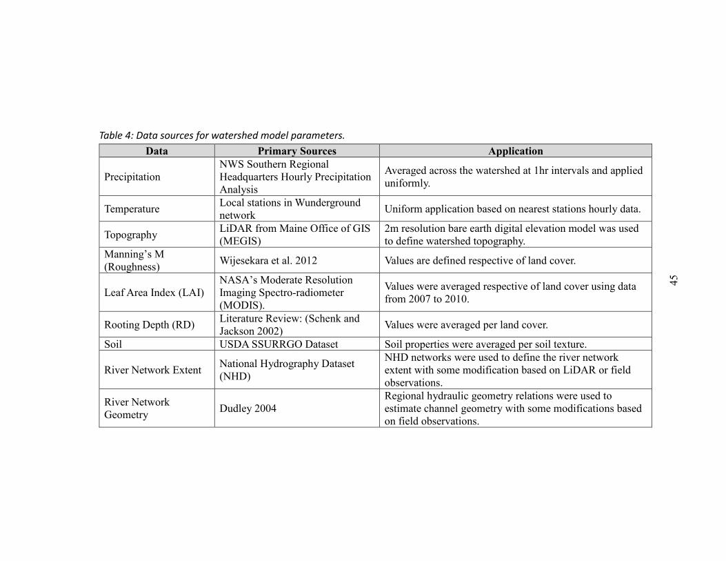
45
Table 4: Data sources for watershed model parameters. Data Primary Sources Application
Precipitation NWS Southern Regional Headquarters Hourly Precipitation Analysis
Averaged across the watershed at 1hr intervals and applied uniformly.
Temperature Local stations in Wunderground network Uniform application based on nearest stations hourly data.
Topography LiDAR from Maine Office of GIS (MEGIS)
2m resolution bare earth digital elevation model was used to define watershed topography.
Manning’s M (Roughness) Wijesekara et al. 2012 Values are defined respective of land cover.
Leaf Area Index (LAI) NASA’s Moderate Resolution Imaging Spectro-radiometer (MODIS).
Values were averaged respective of land cover using data from 2007 to 2010.
Rooting Depth (RD) Literature Review: (Schenk and Jackson 2002) Values were averaged per land cover.
Soil USDA SSURRGO Dataset Soil properties were averaged per soil texture.
River Network Extent National Hydrography Dataset (NHD)
NHD networks were used to define the river network extent with some modification based on LiDAR or field observations.
River Network Geometry Dudley 2004
Regional hydraulic geometry relations were used to estimate channel geometry with some modifications based on field observations.

46
Figure 9: Diagram of the MIKE SHE model platform and the associated principles used to calculate the movement of water for various process.
x
y
Overland Flow: Two-dimensional diffusive wave approximation of the Saint Venant equations (Equations B.1 and B.2)
Saturated Zone: Linear reservoir method (Equation B.5)
Channelized Flow: Fully dynamic Saint Venant equations (Equations B.6 and B.7)
Snow Melt: Degree day melting method (Equations B.8, B.9, and B.10)
Unsaturated Zone: Two-layer water balance method (Yan and Smith 1994) (Equations B.3 and B.4)
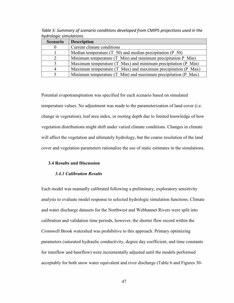
47
Table 5: Summary of scenario conditions developed from CMIP5 projections used in the hydrologic simulations.
Scenario Description 0 Current climate conditions 1 Median temperature (T_50) and median precipitation (P_50) 2 Minimum temperature (T_Min) and minimum precipitation P_Min) 3 Maximum temperature (T_Max) and minimum precipitation (P_Min) 4 Maximum temperature (T_Max) and maximum precipitation (P_Max) 5 Minimum temperature (T_Min) and maximum precipitation (P_Max)
Potential evapotranspiration was specified for each scenario based on simulated
temperature values. No adjustment was made to the parameterization of land cover (i.e.
change in vegetation), leaf area index, or rooting depth due to limited knowledge of how
vegetation distributions might shift under varied climate conditions. Changes in climate
will affect the vegetation and ultimately hydrology, but the coarse resolution of the land
cover and vegetation parameters rationalize the use of static estimates in the simulations.
3.4 Results and Discussion
3.4.1 Calibration Results
Each model was manually calibrated following a preliminary, exploratory sensitivity
analysis to evaluate model response to selected hydrologic simulation functions. Climate
and water discharge datasets for the Northwest and Webhannet Rivers were split into
calibration and validation time periods, however, the shorter flow record within the
Cromwell Brook watershed was prohibitive to this approach. Primary optimizing
parameters (saturated hydraulic conductivity, degree day coefficient, and time constants
for interflow and baseflow) were incrementally adjusted until the models performed
acceptably for both snow water equivalent and river discharge (Table 6 and Figures 30-
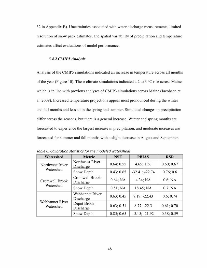
48
32 in Appendix B). Uncertainties associated with water discharge measurements, limited
resolution of snow pack estimates, and spatial variability of precipitation and temperature
estimates affect evaluations of model performance.
3.4.2 CMIP5 Analysis
Analysis of the CMIP5 simulations indicated an increase in temperature across all months
of the year (Figure 10). These climate simulations indicated a 2 to 3 °C rise across Maine,
which is in line with previous analyses of CMIP3 simulations across Maine (Jacobson et
al. 2009). Increased temperature projections appear most pronounced during the winter
and fall months and less so in the spring and summer. Simulated changes in precipitation
differ across the seasons, but there is a general increase. Winter and spring months are
forecasted to experience the largest increase in precipitation, and moderate increases are
forecasted for summer and fall months with a slight decrease in August and September.
Table 6: Calibration statistics for the modeled watersheds. Watershed Metric NSE PBIAS RSR
Northwest River Watershed
Northwest River Discharge 0.64; 0.55 4.65; 1.56 0.60; 0.67
Snow Depth 0.43; 0.65 -32.41; -22.74 0.76; 0.6
Cromwell Brook Watershed
Cromwell Brook Discharge 0.64; NA 4.34; NA 0.6; NA
Snow Depth 0.51; NA 18.45; NA 0.7; NA
Webhannet River Watershed
Webhannet River Discharge 0.63; 0.45 8.19; -22.43 0.6; 0.74
Depot Brook Discharge 0.63; 0.51 8.77; -22.3 0.61; 0.70
Snow Depth 0.85; 0.65 -5.15; -21.92 0.38; 0.59
49
3.4.3 Watershed Scenario Analysis
Flow duration curves were used to compare simulated scenarios for each monitoring site
(Figure 34 in Appendix B). Subtracting the current surface flow rate values from flow
rate values produced by Scenario 1 illustrates patterns of response to climate change
forecasts in the region (Figure 11). Surface water flow changes can be partitioned into
low flow (80- 100% exceedance probability), moderate flow (20- 80% exceedance
probability), and high flow (0- 20% exceedance probability) adjustments.
Simulated low flow discharge rates are predicted to increase within the Webhannet River
and Depot Brook watersheds. The simulated increase in baseflow is a direct result of the
scenario-imposed precipitation increase. This increased precipitation is accompanied by
increases in temperature and evapotranspiration, which leads to a slight decrease in the
very low flow conditions within Northwest River and Cromwell Brook. The effects of
increased evapotranspiration are more pronounced within these systems because of the
greater volume of surface water storage. Examining the water balance reveals that
scenario 1 predicts a 2.5% increase in evapotranspiration within the Webhannet River,
7.5% increase in the Northwest River, and 6.5% increase in Cromwell Brook. In the
Webhannet River watershed, low flows are dominantly supplied by groundwater and not
as effected by the predicted increase in evapotranspiration.
Moderate flows within all three systems are predicted to increase as a results of Scenario
1 climate change conditions. These predicted increases in moderate flow rates are
produced by rainfall events that are modest in depth and intensity compared to historic
records. During these events, precipitation outpaces evapotranspiration and the effect of
50
increased temperature is minimal. The magnitude of change is greatest in Cromwell
Brook, followed by the Northwest and Webhannet Rivers and Depot Brook. This order
correlates with the total surface water storage in each system. These lakes and ponds are
continuously at or near capacity and have limited ability to dampen downstream flows,
acting instead as flow through systems able to sustain these simulated moderate flows. As
these medium sized storms move through the watershed systems, the Great Meadow in
the Cromwell Brook Watershed and the many lakes and ponds throughout the Northwest
River fill above capacity and then slowly drain, producing these moderate flows at that
increase in magnitude with increasing storm intensity.
High flow conditions in all three systems are driven by spring snow melt and/or large,
intense summer storms. CMIP5 analysis predicts that summer precipitation will
minimally increase and simulations in all three watersheds indicate a consistent and
substantial decrease in total snow water equivalent. Accordingly, high flow conditions
appear to remain the same in the Webhannet River watershed, and slightly decrease in the
Northwest River watershed and the Cromwell Brook watershed.
Simulations of snow water equivalent in the Webhannet River produced a unique result
as compared to the Northwest River and Cromwell Brook watersheds. Observed snow
water equivalent in the Webhannet River watershed was comparably less and melted
earlier in the year, likely influenced by the Southern Coastal Maine setting. The
calibration procedure and observed snow dynamics indicate a lower significance of snow
melt contributions to surface flows. Instead, high flows are more related to summer
storms compared to the other watersheds. High flows in the Webhannet River and Depot
Brook are predicted to experience less change under simulated climate conditions for this

51
reason. The effects from climate change remain important in those settings, however,
because small changes to the flow regimes can result in large changes in stream water
discharge volumes and sediment transport.
The Northwest River watershed and the Cromwell Brook watershed experience a some
decrease in peak flows under Scenario 1, a result coupled with reduced snow pack and
warmer weather. However, simultaneous increases in coastal low-pressure systems
resulting from climate change conditions could alter this outcome. A limitation of the
CMIP5 simulations is that they do not account for changes in the frequency of these low-
pressure storm systems moving into the study region from the Mid-Atlantic or Northern
Atlantic Ocean. These weather systems can produce thunderstorms, tropical depressions,
tropical storms, and hurricanes that produce high stream discharge events.
All of the examined watersheds are predicted to experience a decrease in total snow water
equivalent (Figure 12). The magnitude of change is larger for the Webhannet River
watershed, but the pattern of snowpack depletion is similar across all three locations with
a median change for Scenario 1 between 60- 70% of current conditions. This is a
substantial change in total snow water equivalent resulting from increased temperatures
expected through CMIP5 simulations. It should be noted that the delta method does not
account for any change in temperature variance (e.g. warmer days but nighttime
temperature remaining nearly unchanged) which may change total snow water
equivalent.
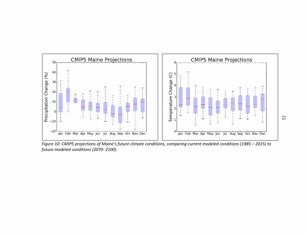
52
Figure 10: CMIP5 projections of Maine’s future climate conditions, comparing current modeled conditions (1985 – 2015) to future modeled conditions (2070- 2100).
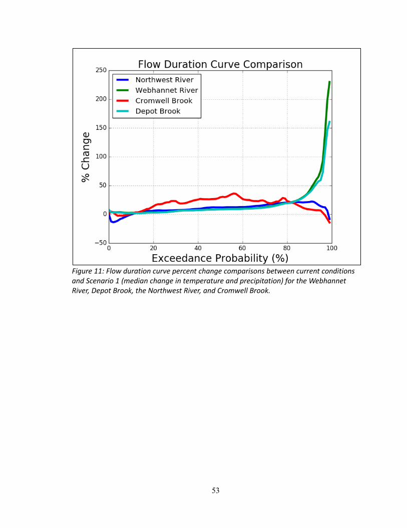
53
Figure 11: Flow duration curve percent change comparisons between current conditions and Scenario 1 (median change in temperature and precipitation) for the Webhannet River, Depot Brook, the Northwest River, and Cromwell Brook.

54
Figure 12: Box and whisker plot presenting the yearly change in total snow water equivalent.

55
Reduced total snow water equivalent is accompanied by a reduction in the number of
days snow is present in the landscape, and the timing of the freshet is consistently earlier
in the year (Figure 13). The simulated increases in temperatures produce similar patterns
in snow melt timing across all three watersheds, with the largest change occurring in the
Webhannet River watershed. Once again, this is a result of the differing snow conditions
along the southern coast of Maine in comparison to the Lakes Region and Mid-Coast.
Based on the median expected shift in temperature and precipitation from CMIP5
simulations, these model results indicate a potential shift in the timing of snow melt
termination of between 10 and 20 days for the Central and Coastal Maine region.
The combined outcome of the projected climate conditions is a shift in the characteristic
flow regime for the three watersheds (Figure 14). The most prominent change to the flow
regime is a shift in the seasonally high flows resulting from the melting of the winter
snow pack. Scenario 1 climate conditions result in these seasonally high flows occurring
earlier in the year, and throughout the remainder of the year we see less change, although
some decreases in flow are more notable in the Northwest River system (Figure 14).
3.5 Conclusions
The parameterization and calibration of three Coastal and Central Maine watershed
models provided a tool for the examination and comparison of climate change conditions
in varied watershed settings. Although hydrologic simulation results have limited ability
to predict future conditions with high accuracy, the results describe the magnitude and
characteristics of stream flow regime alterations linked to climate conditions. The
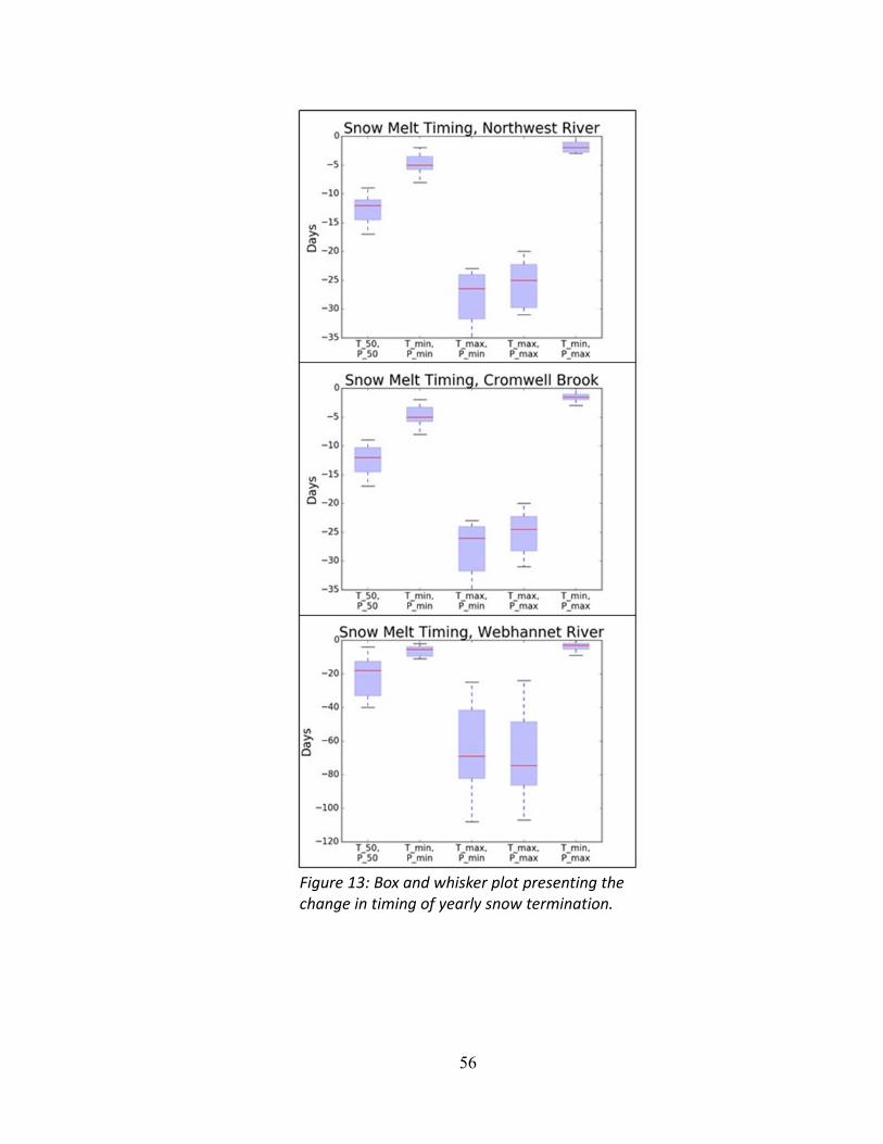
56
Figure 13: Box and whisker plot presenting the change in timing of yearly snow termination.

57
analytical outcomes quantify how surface flow patterns associated with climate change
forecasts vary relative to the collection of watershed processes controlling watershed
runoff production and routing. Although some generalizations can be made in the region,
the varied responses predicted from the simulations show how the effects from climate
change effects will differ relative to local watershed conditions in the Northeast. The
observations highlight the varied vulnerability of stream system and associated
biophysical-ecological processes to the effects of climate change. Localized responses of
stream systems will be dependent on the physiography, landscape history, human
activities, surface water resource management activities, and modern land uses.
Figure 14: Hydrologic signature for Northwest River representing the change in timing and magnitude of flow between current conditions and Scenario 1 (median precipitation and temperature change).
58
CMIP5 climate simulations indicate a continuing increase in annual temperature and
increases in winter, spring, and fall precipitation over the next century. The forecast
conditions shift the total average snow water equivalent and snow melt timing. Total
snow water equivalent decreases and the timing of snow melt occurs ten to twenty days
earlier in the year. This causes the characteristically high spring flows to change in terms
of timing (earlier) and magnitude (lower), supporting similar results found through
historical analysis by Hodgkins and Dudley (2006). Other flow regime modifications
resulted from increased precipitation and evapotranspiration with variability related to
upland water storage capacity.
The findings suggest that biophysical-ecological process closely tied to snowpack and
snowmelt processes are the most vulnerable to climate change in the region. The
observed relevance of surface water storage to stream flow conditions highlights that
drainage routing dynamics in lakes and ponds should be an important consideration when
deciding where and how water resource sustainability efforts should be focused. The
potential effects of surface water storage in the landscape increases moderate flows but
appear to “buffer” the highest of flows, suggesting that locations downstream of these
features may be less vulnerable to scour from high flow events resulting from projected
increases in runoff from altered precipitation and snowpack inputs.
The research outcomes provide a foundation for identifying a strategy for surface water
resource management in the post-glaciated Northeast region. The predicted changes to
flow regime have important implications to ecosystem services provided by natural
waterways that govern water quality conditions (Arthington et al. 2010). Changes to
surface flow regime will alter terms in the sediment-water proportionality governing
59
stream system dynamics and nonpoint source pollutant transport into large rivers, lakes,
and estuaries in Maine. Results from this work suggest that water resource management
strategies should consider the local physiographic and land use conditions.
3.6 Acknowledgements
The research described in this chapter was funded by the Maine Water Resources
Research Grants Program (Project Number: 5406025) and two National Science
Foundation EPSCoR projects: 1) Maine’s Sustainability Solutions Initiative (National
Science Foundation award EPS-0904155); and 2) New England Sustainability
Consortium (National Science Foundation award IIA-1330691). In addition to review
and input from committee members, I’d like to thank Ying Qiao. She was instrumental in
assisting with the parameterization and calibration of these models. I’d also like to thank
Shaleen Jain and Sean Birkel for their help and guidance evaluating climate change
projections. Thank you also to the many students who provided constant support through
field data collection and various GIS analyses.
60
CHAPTER FOUR
NORTHEASTERN HEADWATER STREAM BED DYNAMICS UNDER VARIED
CLIMATE CONDITIONS
4.1 Chapter Abstract
The geomorphology of Northern New England is a product of geologic, glacial, and
anthropogenic processes operating over a range of time scales. Better knowledge and
information about the impact of these processes, particularly the effects of human
activities, on the physical condition of modern stream systems is necessary for the
development of watershed management and restoration strategies. Research on coupled
human-climate-stream systems in the region is limited despite the importance to
sustainability solutions for surface water quality and aquatic habitat problems.
Information gaps persist on headwater stream channel dimensions and dynamics in varied
settings of Maine even though they compose the majority of drainage network lengths.
This project responded to the information gap by focusing on headwater stream
hydraulics and geomorphology in fluvial systems of variable landscape characteristics
across Central and Coastal Maine to support the development of watershed management
decision tools. Research results improve characterization of upland stream channel
dimensions and expand the capacity to predict stream responses to physiography, land
use, and climate changes. Comparison of upland channels to those in lowland “alluvial”
valley settings improves information customizing management responses to multi-
objective stream management and engineering problems.

61
The analyses describe and quantify regional relations between in-channel conditions and
watershed processes linked to deglaciation processes, land cover, and human activities in
the region. The approach combines field measurements of stream channel dimensions
with surface flow time series derived from watershed hydrologic simulations in multiple
settings defined by relief, surficial geology, and land uses. Hydraulic geometry
measurements describing upland channel dimensions are compared to predictive
geometry measurements derived from previous measurements of lowland stream
channels in the region (Dudley 2004).
The analysis shows relatively greater variability in upland channel dimensions compared
to streams in lowland valleys that were measured by others to develop predictive
relations. Predictive hydraulic geometry relations developed from streams set in lowland
valleys differ minimally from those in upland settings but do generally under-predict the
dimensions of upland streams surveyed as part of this project. The difference in the
hydraulic geometry relations indicates the operation of a unique set of processes
governing stream dimensions in modern upland and lowland settings.
Analyses of channel bed sediment transport using sediment grain size measurements,
upland stream channel dimension data, and surface flow time series derived from
watershed simulations provide another means to evaluate stream responses to watershed
and climate conditions. Watershed hydrology simulations included climate change
scenarios to compare stream responses to forecasted conditions impacting stream flows in
the region. Sediment bedload transport analyses indicated changes which varied across
watershed settings and climate conditions. Streams receiving flows from watersheds with
relatively low surface water storage capacity responded with a measurable increase in
62
sediment mobility, and a decrease in mobility was detected in stream reaches downstream
from locations with relatively large amounts of surface water storage capacity. Overall,
the results present the range of stream system responses to forecasted climate changes
and demonstrate the relevance of watershed conditions to those responses.
4.2 Introduction
Surface runoff dynamics and the supply of sediment in the modern topography of Maine
are influenced by the historical advance and retreat of the Laurentide Ice Sheet
approximately 15 Kya (Borns Jr et al. 2004). The conditions of the modern landscape
partly defined by this glacial history govern the sediment-water proportionality within
watersheds across the region. The competence of surface flows to transport the relatively
large clast sizes deposited during deglaciation of the region and now observed in stream
channels is inadequate, resulting in a low frequency of sediment transport events in many
drainage network locations (Snyder et al. 2009). The capacity of headwater stream flows
is also often high relative to the supply of fine sediment in the landscape due to
mechanical erosion of regolith by glacial processes. Local conditions exhibit some
inconsistencies with these regional characteristics where glacially derived landforms such
as eskers produce locations of elevated sediment supply. The region also exhibits a
prominent transition in surficial geology related to the submergence of the eastern portion
of Maine as the Laurentide Ice Sheet retreated (Borns et al. 2004). This marine
transgression produced a till dominated surficial geology in central and inland portions of
the state and a marine dominated surficial geology with finer grained sediment along the
coast. These conditions have created both localized and regional variations in the supply
of sediment to streams.

63
Modern drainage network conditions in the region are additionally a product of
subsequent European colonization of the region starting in the early 1600’s (Maine
Historical Society 2014). Colonization introduced large-scale and small-scale industrial
activities (e.g. agriculture, forestry, mills, etc.) that involved physical alterations to
streams and river valleys (e.g. run-of-the-river dams, splash dams, and channelization of
stream channels, etc.) (Allen 2013). These activities further impacted Maine’s watershed
systems by indirectly changing the supply of water and sediment. Many of the physical
effects from these activities are less apparent today, but their impacts on the modern
drainage network persist.
These activities occurring over a range of time scales define the sediment-water dynamics
of the landscape and govern modern stream dimensions, slope, water discharge, and
sediment load. Channel conditions are responding to the balance between the sediment
supply and stream flow capacity to transport that supply through a reach given the
associated hydraulic conditions (Lane 1955) (Figure 1 and Equation 3). This relation is
described by the proportionality given by Henderson (1989):
𝑞𝑞𝑠𝑠𝐷𝐷32 ∝ (𝑞𝑞𝑄𝑄)2 [13]
where D is sediment size, S is channel slope, and 𝑞𝑞𝑠𝑠 and 𝑞𝑞 are the sediment transport rate
per unit width and discharge per unit width, respectively. Rearranging Equation 13
expresses the relation of 𝑞𝑞𝑠𝑠, 𝑞𝑞, and 𝐷𝐷 to changes in channel dimensions through
aggradation or degradation over time (𝑅𝑅1𝑅𝑅2
) (Wilcock et al. 2009):

64
𝑄𝑄1𝑄𝑄2
= (𝑞𝑞𝑠𝑠2𝑞𝑞𝑠𝑠1
)12(𝑞𝑞1𝑞𝑞2
)(𝐷𝐷2𝐷𝐷1
)34 [14]
Stream dynamics driven by the sediment-water proportionality are of significant interest
to multiple stakeholders in the region, particularly as they relate to future conditions and
responses to watershed land use and climate changes. A prominent focus is the
sustainability of in-stream habitat and downstream water quality because of the
association with ecosystem services. Examples of sustainability solutions to related
problems include stream restoration projects, multi-objective stream culvert designs,
stormwater management for control of surface water discharge rates, and the
management of nonpoint source pollutants such as sediment and nutrients.
The research summarized here examines the modern sediment-water dynamics governing
stream channel conditions and evaluates the effects of forecasted climate changes to
provide information and decision tools in support of modern stream system management
challenges in the Northeast. This research leverages the conventions developed to
quantify channel hydraulic geometry (Leopold and Maddock 1953) and builds on more
recent regional observations describing channel conditions in Coastal and Central Maine
watersheds by Dudley (2004). Existing channel geometry information derived from
measurements by Dudley (2004) in lowland streams is compared to new measurements
collected from headwater streams, providing valuable information for water resource
management applications such as stream restoration and culvert design in upland
headwater drainage networks. Sediment dynamics within headwater stream systems
under projected climate conditions are examined to quantify the impact of altered flow

65
conditions on channel hydraulics and dynamics. The analyses of dynamics focuses on
sediment transport in varied landscape settings, examining the magnitude and spatial
variability of future adjustment to predicted discharge time series. The outcomes inform
and guide implementation of water resource management strategies in locations that have
been impacted by modern human interventions or that are vulnerable to forecasted
climate change effects on watershed surface runoff.
4.3 Methods
4.3.1 Data Collection
Geospatial data was assembled, and channel measurements were collected from 45
stream reaches within five watersheds in Central and Coastal Maine. These watersheds
are the Sebago Lake watershed in the Maine Lakes Region (n = 34), the Webhannet River
watershed along the Southern Coast (n = 6), the Cromwell Brook watershed in Mid-Coast
Maine (n = 3), the Damariscotta Estuary watershed between the Southern Coast and Mid-
Coast (n = 1), and the Bear Brook watershed in the Downeast Region of Maine (n = 1).
Stream measurements included topographic surveys of channel cross sections and water
surface slopes at baseflow conditions. Pebble counts were conducted to estimate bed
grain size distributions (Wolman 1954) and corresponding watershed drainage areas were
estimated using digital elevation data from available online sources (Maine Office of GIS
2017).
Headwater stream reaches in the study watersheds were selected to consider a range of
stream conditions described by channel dimension (size), profile (slope), bottom
sediment composition (grain size), riparian corridor conditions (vegetation), watershed
conditions (land cover, soils, and topography), and history of disturbance from humans
66
(e.g., presence of dams and culverts). These primary data collection sites were coupled
and compared to information from previous investigations by the USGS (Dudley 2004)
and results from the Instream Flow Incremental Methodology (IFIM) evaluations in the
region (Kleinschmidt 1999a, 1999b).
4.3.2 Hydraulic Geometry
Hydraulic geometry addresses the fundamental relations between discharge, flow
velocity, and channel dimensions in alluvial settings (Leopold and Maddock 1953). The
relations can be expressed for a single station over a range of discharge rates (and
corresponding flow stages) with an “at-a-station” geometry approach; or, for multiple
stations representing upstream to downstream increases in bankfull discharge and
corresponding flow dimensions with progressively larger contributing drainage area. The
relations are expressed as the following functions with either approach:
𝑤𝑤 = 𝑎𝑎𝑄𝑄𝑏𝑏 [15]
𝑑𝑑 = 𝑐𝑐𝑄𝑄𝑓𝑓 [16]
𝑣𝑣 = 𝑘𝑘𝑄𝑄𝑚𝑚 [17]
where Q is streamflow, w is channel width, d is channel depth, v is flow velocity, and a,
c, and k are derived coefficients, while b, f, and m are derived exponents. Because
discharge is a function of cross section area (depth × width) and velocity, the exponents
of these relations sum to one and the product of the coefficients equal one.
Downstream hydraulic geometry was evaluated relative to the channel bankfull
dimensions, boundaries of which are determined in the field using features such as the

67
top of the bank, outer edges of point bars, depositional deposits (benches), and/or changes
in substrate and vegetation (Williams 1978; Harrelson et al. 1994). The relations were
evaluated longitudinally in portions of drainage networks traversing through upland
hillslopes sculpted by glacial processes and lowland alluvial valleys with floodplain
deposits. At-a-station relations were defined using a meta-data analysis incorporating
primary survey sites and four IFIM study sites from larger streams. Because of
incomplete flow records for many of these locations, this research used a modified
approach to examine at-a-station geometry focused on the ratio of the channel width to
depth as a function of discharge or drainage area (DA).
𝑤𝑤𝑑𝑑
= 𝑗𝑗(𝐷𝐷𝐷𝐷)𝑟𝑟 [18]
While this relation does not fully express how a channel accommodates increasing flows
at a given cross-section, principally because it does not consider stream flow velocity, it
does provide useful information regarding channel shape, dimensions, and the relative
change in channel width and depth as flows increase at a cross-section.
4.3.3 Sediment Entrainment Frequency
Observations suggest that rates of sediment transport in the study region are generally
low compared to non-glacial landscapes of the U.S.A. (Leopold et al. 1995; Snyder et al.
2009; Wilcock et al. 2009). Much of the sediment that is transported in the Central and
Coastal Maine landscape is dominated by bedload with a majority of the grains moving
along or near the streambed. Suspended and wash loads transported within the water

68
column are a less significant portion of the total load in the region (Leopold et al. 1995;
Wilcock 2009). The dominance of bed-material transport is largely driven by the limited
supply of fine material resulting from limited fine-grained regolith in the landscape
following the most recent advance and retreat of the Laurentide ice sheet (Ferwerda et al.
1997). For this reason, this research focuses specifically on bed-material transport.
Channel bed dynamics in coarse-bedded stream systems similar to those in Maine are
largely controlled by the initiation of motion of the surface layer (Wilcock and Crowe
2003). This is because the vertical sorting of bed sediments produces a surface layer
coarser than the substrate, causing high rates of transport be associated with movement in
the surface layer. The approach used here is thereby focused on the flow competence
problem to evaluate the frequency of bed material motion.
Incipient motion conditions, at which bed material becomes mobile, was evaluated from
sediment transport calculations. Incipient motion conditions were considered to have
been met once a small fraction, 1%, of the sediment quantile’s mass was transported in
one unit (minute) of time. The discharge at which these conditions were met or exceeded
was compared to current and projected flow conditions from previous research (Chapter
3). Calculations were made for the Northwest River, Webhannet River, Cromwell Brook,
and Depot Brook.
At each location and for each climate scenario flow condition, fractional transport rates of
sediment within each grain size range (phi interval) were calculated using the surface-
based Wilcock and Crowe (2003) (Equation 19) transport model implemented through
the Bedload Assessment in Gravel-bedded Streams (BAGS) program:

69
𝑑𝑑𝑖𝑖 =
𝜏𝜏𝑔𝑔𝜏𝜏𝑟𝑟𝑠𝑠𝑔𝑔
(𝐷𝐷𝑠𝑠𝑔𝑔𝐷𝐷𝑖𝑖
)χ [19]
where 𝑑𝑑𝑖𝑖 is the dimensionless fractional transport rate, 𝜏𝜏𝑟𝑟𝑠𝑠𝑔𝑔 is the reference shear stress
for the mean grain size, 𝐷𝐷𝑠𝑠𝑔𝑔 is the mean grain size for the gravel portion of the bed, and χ
varies relative to grain size ratio 𝐷𝐷𝑖𝑖/𝐷𝐷𝑠𝑠𝑔𝑔. The use of this surface-based model decreased
the logistical difficulties of sub-surface sampling, particularly in deeper rivers, and its
explicit treatment of sand is well suited for the sandy nature of many streams throughout
the study region.
Calculated transport rates were compared to channel geometry measurements,
measurements of channel bed sediment composition, and modeled flow conditions to
estimate the frequency at which the D50 (median), D16, and D84 grain sizes in each stream
are mobile, the latter two of which represents the smallest and largest portions of the
measured grain size distributions. The mass of each sediment quantile (i.e. D16, D50, and
D84) was estimated within a unit length of each stream using the observed channel width,
the sediment distribution, an estimated depth equal to the sediment quantile’s value, and
the density of granite (2.65g/cm3).
4.4 Results and Discussion
4.4.1 Hydraulic Geometry
A log-log plot of drainage area versus channel slope shows a visual inflection of the
relation at approximately 1 km2 for primary and secondary study sites (Figure 15).
Montgomery and Buffington (1997) presented a similar inflection in this relation at
70
approximately the same drainage area for mountain streams of the western USA,
suggesting that this presented the transition from threshold to alluvial channels. Field
observations generally support the occurrence of stream channel transitions from
threshold to alluvial channels at drainage areas of approximately 1 km2 in Maine.
However, the primary driver of the relation and inflection in the trend may be unique to
the Maine landscape and related to processes associated with landforms created by glacial
advance and retreat in the region.
Field measurements of bankfull channel dimensions generally conform to downstream
geometry relations developed on larger, lowland channels in the Central and Coastal
Maine region (Dudley 2004). However, while the previously published relations provide
reasonably accurate predictions of geometry in the largest channels of our dataset, the
relations result in progressively greater under-prediction of channel width and depth with
smaller contributing drainage areas. Under-prediction is most observed for channel depth
(Figure 16). Observations of low sediment supply in the landscape lead to the assumption
that the hydraulic geometry of the upland headwater channels can be attributed to the
imbalance between sediment supply and flow capacity, producing incised channels that
do not recover from erosion events through subsequent infill with new sediment from
upslope sources.
At-a-station geometry calculations reveal a gradual transition from more confined, v-
shaped channel conditions to more unconfined, rectangular shaped channels with
increasing drainage area (Figure 17). Results also indicate that headwater streams exhibit
much greater variability in channel shape. Localized structural (geologic) controls and
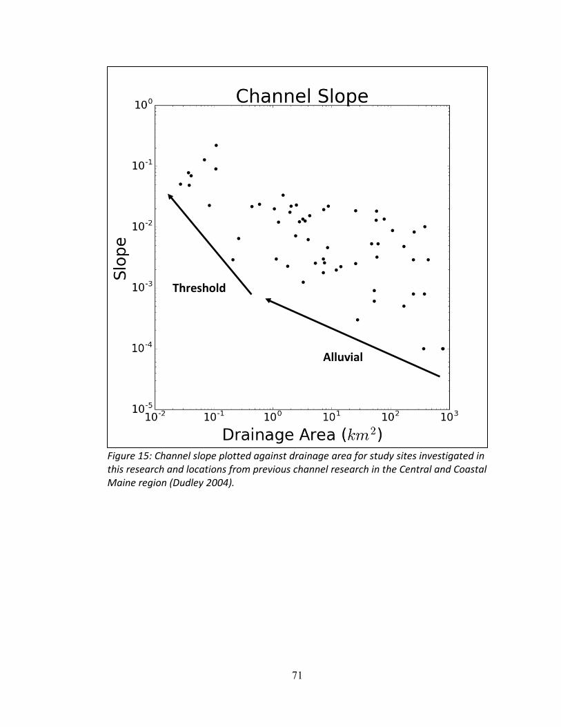
71
Figure 15: Channel slope plotted against drainage area for study sites investigated in this research and locations from previous channel research in the Central and Coastal Maine region (Dudley 2004).
Alluvial
Threshold

72
Figure 16: Downstream hydraulic geometry relations from this study, in blue, plotted against previous results from the region, in black (Dudley 2004).
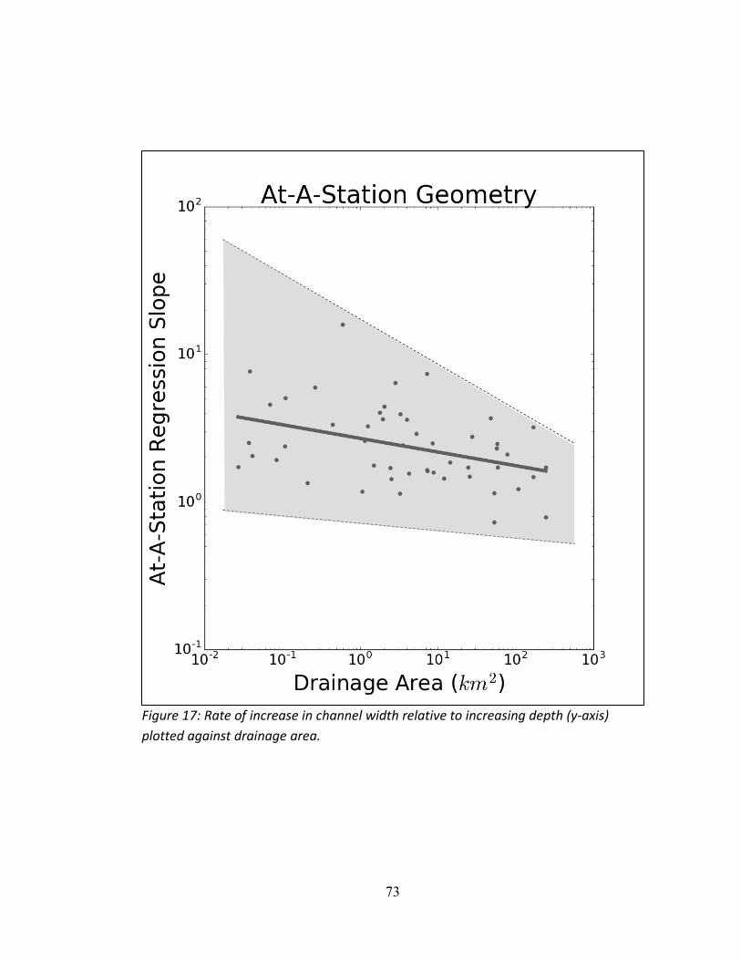
73
Figure 17: Rate of increase in channel width relative to increasing depth (y-axis) plotted against drainage area.
74
changes to channels and their contributing drainage areas by humans offer plausible
explanations for the observed inconsistencies in the dimensions and shapes. Field and
watershed reconnaissance observations support the conclusion that localized features and
disturbances have considerable influence on modern headwater stream conditions.
4.4.2 Sediment Entrainment and Load Estimation
Estimated changes in the frequency of bed sediment entrainment generally align with the
imposed climate conditions used to derive the flow regime scenarios (Table 7; Where
Scenario 1 represents the median forecasted changes in temperature and precipitation;
Scenario 2 represents the minimum forecasted changes in temperature and precipitation;
Scenario 3 represents the maximum forecasted changes in temperature and minimum
forecasted changes in precipitation; Scenario 4 represents the maximum forecasted
changes in temperature and precipitation; Scenario 5 represents the minimum forecasted
changes in temperature and maximum forecasted changes in precipitation). Across all
four locations, Scenarios 2 and 3 produce a substantial decrease in the frequency of
sediment mobility. These scenarios were developed using the lowest forecasted monthly
average precipitation from CMIP5 ensembles. Across all months, the minimum projected
precipitation was lower than current conditions, resulting in lower simulated stream
flows. Scenarios 4 and 5, which forecast the maximum average monthly precipitation
from CMIP5 projections, produced a significant increase in the frequency of sediment
transport across all four locations. Precipitation in these scenarios is substantially higher
than current conditions and this effect is propagated to the sediment entrainment
estimates.
75
Scenario 1 flow conditions, produced from the median forecasted precipitation and
temperature changes indicated by the CMIP5 ensemble, results in varied outcomes across
the study sites. Predicted increases in precipitation drives greater frequency of bed
material mobilization for all size classes at Depot Brook and the Webhannet River. More
variable outcomes were observed in the Northwest River and Cromwell Brook locations.
Flow conditions that initiate particle motion of smaller grain sizes (represented by D16
sizes) remain nearly unchanged in the Northwest River and decrease slightly for
Cromwell Brook. The D50 sediment particle sizes show a slight decrease and no change
for the Northwest River and Cromwell Brook, respectively (movement of the 𝐷𝐷80 in the
Northwest River is very small in comparison to other size classes, and the increase in
Table 7 would have relatively little effect on channel bottom conditions). These
observations in the mobilization frequency for the Northwest River and Cromwell Brook
are likely a function of decreasing snow melt contributions to flow and related to the
substantial surface water storage in these watersheds. Watershed model calibration
procedures and observed snow dynamics indicated a higher significance of snow melt
contributions to surface flows at these watersheds as compared to the Webhannet River
watershed. Furthermore, both locations have substantial surface water storage in wetlands
and ponds that may moderate surface flow rates produced from increases in precipitation
and temperature. Increased temperatures drive up evapotranspiration, which increases
available storage capacity and may buffers storm flows. However, observations of static
or decreases in transport frequency may be affected by weaknesses in the climate change
scenarios. Climate change scenarios were developed using the delta method in
conjunction with projected shifts in temperature and precipitation from CMIP5

76
projections. This method uses historical climate data and adds or subtracts the projected
change in each variable, it does not factor into account possible changes in the frequency
of rainfall events. Furthermore, CMIP5 projections are limited in their representation of
tropical storm events, which could influence future summer climate conditions in the
study region. Those locations and size classes most frequently mobilized during summer
storm events are not well represented by the climate scenarios used for the hydrologic
simulations.
Table 7: Predicted percent change in the frequency of bed material entrainment relative to current conditions. Dash indicates mobilization not estimated under current conditions.
4.5 Conclusions
Downstream hydraulic geometry relations constructed from upland headwater steams in
the study region are generally similar to those developed from larger regional lowland
river channels, with the primary exception of channel depth. The relation developed by
Dudley (2004) under-predicts channel depth for the smallest streams measured in this
study, likely due to the low sediment supply relative to the transport capacity in these
headwater upland stream channels. As in other physiographic settings, headwater
channels in Maine do not recover from scour events because of inadequate upstream
sediment supply. This contrasts with stream channels within lowland alluvial valleys,
D16 D50 D84 D16 D50 D84 D16 D50 D84 D16 D50 D84
Grain Size (mm) 50 114 256 2 30 91 8 20 40 4 42 82Scenario 1 0% -33% 80% 11% 7% - -17% 0% - 5% 25% 100%Scenario 2 -43% -61% -100% -39% -52% - -75% -100% - -40% -75% -100%Scenario 3 -60% -81% -100% -43% -50% - -75% -100% - -42% -63% -100%Scenario 4 61% 29% 600% 110% 117% - 208% 350% - 109% 163% 300%Scenario 5 89% 85% 1020% 117% 124% - 233% 400% - 107% 200% 200%
Northwest River Cromwell BrookWebhannet River Depot Brook
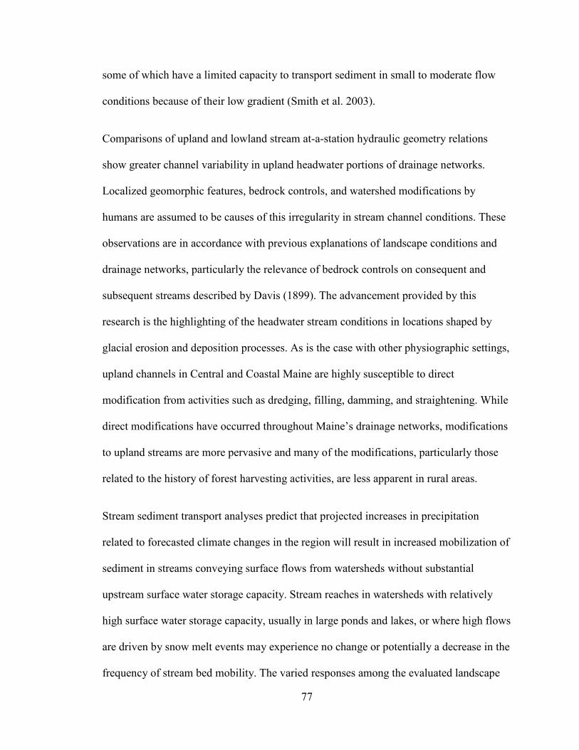
77
some of which have a limited capacity to transport sediment in small to moderate flow
conditions because of their low gradient (Smith et al. 2003).
Comparisons of upland and lowland stream at-a-station hydraulic geometry relations
show greater channel variability in upland headwater portions of drainage networks.
Localized geomorphic features, bedrock controls, and watershed modifications by
humans are assumed to be causes of this irregularity in stream channel conditions. These
observations are in accordance with previous explanations of landscape conditions and
drainage networks, particularly the relevance of bedrock controls on consequent and
subsequent streams described by Davis (1899). The advancement provided by this
research is the highlighting of the headwater stream conditions in locations shaped by
glacial erosion and deposition processes. As is the case with other physiographic settings,
upland channels in Central and Coastal Maine are highly susceptible to direct
modification from activities such as dredging, filling, damming, and straightening. While
direct modifications have occurred throughout Maine’s drainage networks, modifications
to upland streams are more pervasive and many of the modifications, particularly those
related to the history of forest harvesting activities, are less apparent in rural areas.
Stream sediment transport analyses predict that projected increases in precipitation
related to forecasted climate changes in the region will result in increased mobilization of
sediment in streams conveying surface flows from watersheds without substantial
upstream surface water storage capacity. Stream reaches in watersheds with relatively
high surface water storage capacity, usually in large ponds and lakes, or where high flows
are driven by snow melt events may experience no change or potentially a decrease in the
frequency of stream bed mobility. The varied responses among the evaluated landscape
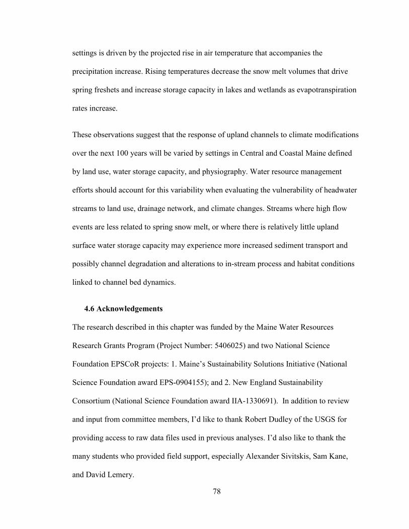
78
settings is driven by the projected rise in air temperature that accompanies the
precipitation increase. Rising temperatures decrease the snow melt volumes that drive
spring freshets and increase storage capacity in lakes and wetlands as evapotranspiration
rates increase.
These observations suggest that the response of upland channels to climate modifications
over the next 100 years will be varied by settings in Central and Coastal Maine defined
by land use, water storage capacity, and physiography. Water resource management
efforts should account for this variability when evaluating the vulnerability of headwater
streams to land use, drainage network, and climate changes. Streams where high flow
events are less related to spring snow melt, or where there is relatively little upland
surface water storage capacity may experience more increased sediment transport and
possibly channel degradation and alterations to in-stream process and habitat conditions
linked to channel bed dynamics.
4.6 Acknowledgements
The research described in this chapter was funded by the Maine Water Resources
Research Grants Program (Project Number: 5406025) and two National Science
Foundation EPSCoR projects: 1. Maine’s Sustainability Solutions Initiative (National
Science Foundation award EPS-0904155); and 2. New England Sustainability
Consortium (National Science Foundation award IIA-1330691). In addition to review
and input from committee members, I’d like to thank Robert Dudley of the USGS for
providing access to raw data files used in previous analyses. I’d also like to thank the
many students who provided field support, especially Alexander Sivitskis, Sam Kane,
and David Lemery.

79
CHAPTER FIVE
DECISION SUPPORT FOR SURFACE WATER RESOURCE SUSTAINABILITY
IN POST-GLACIAL LANDSCAPES
5.1 Chapter Abstract
The implementation of adaptive management strategies for water resource sustainability
in the Northeastern USA requires an understanding of the dynamic interactions between
the region’s post-glacial landscape and headwater stream systems. The majority of
stream network length is comprised of these headwater systems that provide important
ecological functions and govern the conditions in downstream lowland rivers, lakes, and
estuaries. Regional stakeholder concerns focused on the sustainability of potable drinking
water quality, safe civil infrastructure, economically important recreation and tourism
activities, resilient aquatic habitat conditions, and viable coastal fisheries are ultimately
influenced by the inseparable and dynamic interactions between the landscape and upland
surface flows and stream bed conditions. Accordingly, this research targeted hydrologic
and sediment dynamics governing headwater stream conditions to provide information to
guide the development and implementation of adaptive management strategies.
The questions and objectives of this research, which have been addressed as individual
research components relating to watershed conditions, channel hydrology, and channel
morphology, were organized to provide a framework to support water resource
sustainability solutions. The organization of this research was developed through the
identification of problems and co-generation of knowledge with stakeholder
communities, reviews of a diverse collection of background information, and assembly of
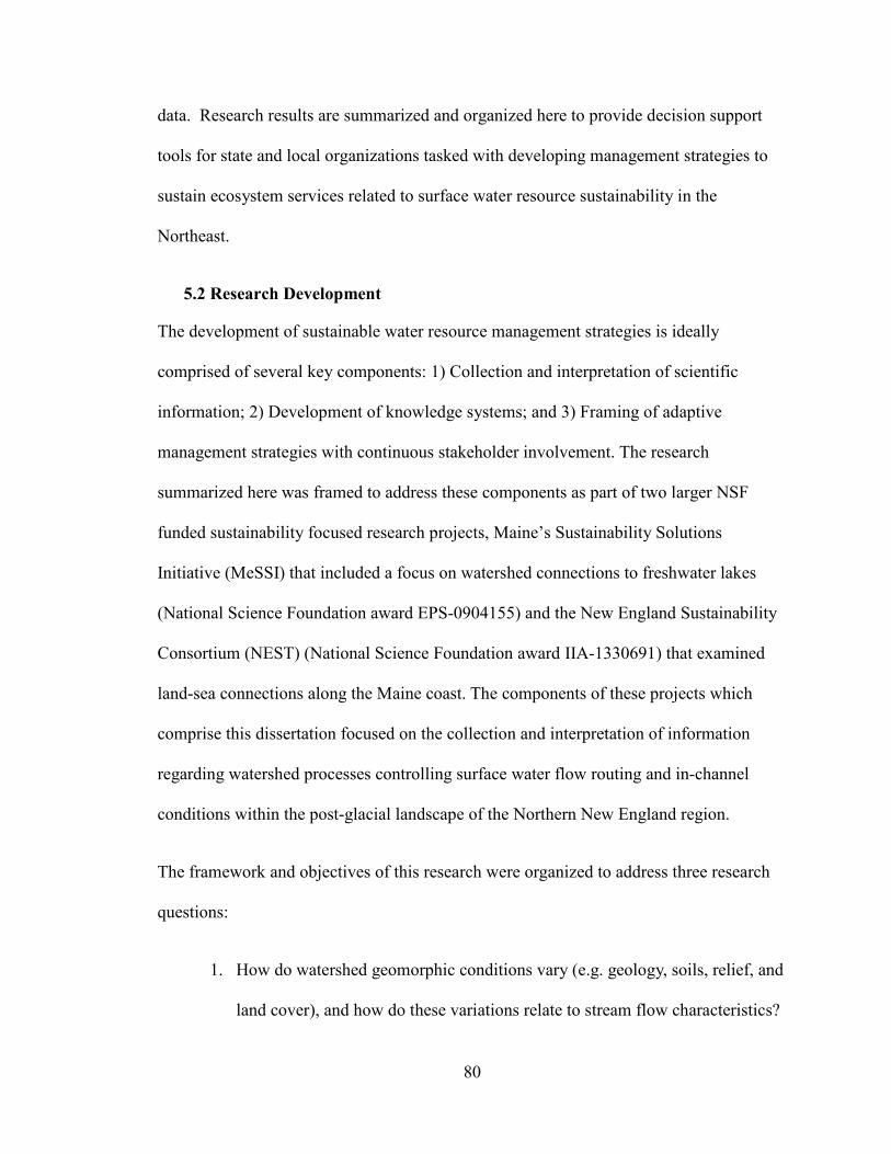
80
data. Research results are summarized and organized here to provide decision support
tools for state and local organizations tasked with developing management strategies to
sustain ecosystem services related to surface water resource sustainability in the
Northeast.
5.2 Research Development
The development of sustainable water resource management strategies is ideally
comprised of several key components: 1) Collection and interpretation of scientific
information; 2) Development of knowledge systems; and 3) Framing of adaptive
management strategies with continuous stakeholder involvement. The research
summarized here was framed to address these components as part of two larger NSF
funded sustainability focused research projects, Maine’s Sustainability Solutions
Initiative (MeSSI) that included a focus on watershed connections to freshwater lakes
(National Science Foundation award EPS-0904155) and the New England Sustainability
Consortium (NEST) (National Science Foundation award IIA-1330691) that examined
land-sea connections along the Maine coast. The components of these projects which
comprise this dissertation focused on the collection and interpretation of information
regarding watershed processes controlling surface water flow routing and in-channel
conditions within the post-glacial landscape of the Northern New England region.
The framework and objectives of this research were organized to address three research
questions:
1. How do watershed geomorphic conditions vary (e.g. geology, soils, relief, and
land cover), and how do these variations relate to stream flow characteristics?
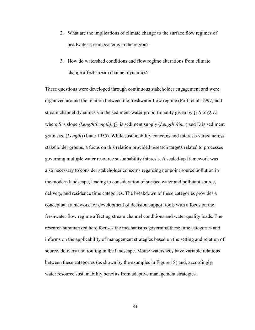
81
2. What are the implications of climate change to the surface flow regimes of
headwater stream systems in the region?
3. How do watershed conditions and flow regime alterations from climate
change affect stream channel dynamics?
These questions were developed through continuous stakeholder engagement and were
organized around the relation between the freshwater flow regime (Poff, et al. 1997) and
stream channel dynamics via the sediment-water proportionality given by Q S ∝ Qs D,
where S is slope (Length/Length), Qs is sediment supply (Length3/time) and D is sediment
grain size (Length) (Lane 1955). While sustainability concerns and interests varied across
stakeholder groups, a focus on this relation provided research targets related to processes
governing multiple water resource sustainability interests. A scaled-up framework was
also necessary to consider stakeholder concerns regarding nonpoint source pollution in
the modern landscape, leading to consideration of surface water and pollutant source,
delivery, and residence time categories. The breakdown of these categories provides a
conceptual framework for development of decision support tools with a focus on the
freshwater flow regime affecting stream channel conditions and water quality loads. The
research summarized here focuses the mechanisms governing these time categories and
informs on the applicability of management strategies based on the setting and relation of
source, delivery and routing in the landscape. Maine watersheds have variable relations
between these categories (as shown by the examples in Figure 18) and, accordingly,
water resource sustainability benefits from adaptive management strategies.
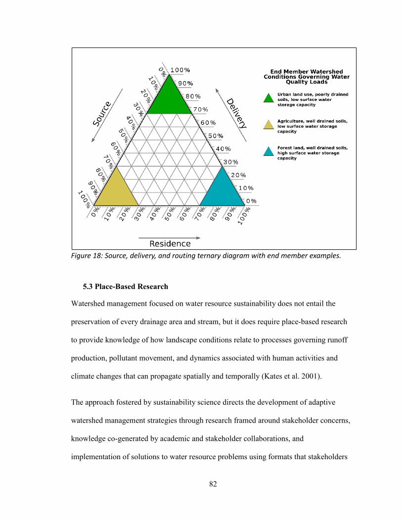
82
Figure 18: Source, delivery, and routing ternary diagram with end member examples.
5.3 Place-Based Research
Watershed management focused on water resource sustainability does not entail the
preservation of every drainage area and stream, but it does require place-based research
to provide knowledge of how landscape conditions relate to processes governing runoff
production, pollutant movement, and dynamics associated with human activities and
climate changes that can propagate spatially and temporally (Kates et al. 2001).
The approach fostered by sustainability science directs the development of adaptive
watershed management strategies through research framed around stakeholder concerns,
knowledge co-generated by academic and stakeholder collaborations, and
implementation of solutions to water resource problems using formats that stakeholders

83
are comfortable using. Clearly parsing problems into relevant spatial and temporal scales
and evaluating vulnerability relative to that organizational structure is a substantial front
end of water resource sustainability solutions work. The initial question guiding this
research address the place-based aspect of sustainability research by examining landscape
heterogeneity related to the mechanics of runoff production and routing in headwater
drainage networks.
The region’s geomorphology and history of alteration by humans has created a complex
array of watershed conditions and settings in which communities, environmental
organizations, and government organizations such as the Portland Water District (PWD)
and the Maine Department of Marine Resources (MEDMR) implement water resource
management strategies targeting stream ecosystem services. Stakeholder engagement at
the beginning of this project guided a systematic delineation of locations with relatively
high susceptibility to water resource problems linked to stream flows, hydraulics, and
sediment-water dynamics.
While there is a general interest in watershed management strategies customized relative
to specific conditions and settings, two groups of stakeholders had substantial influence
on the approach. Communities and organizations concerned with Maine’s largest public
drinking water supply, Sebago Lake, inspired the examination of locations in the
Presumpscot River watershed with relatively greater vulnerability to climate and land use
changes affecting in-stream processes linked to surface water quality conditions.
Communities, industries, and government agencies along the coast similarly expressed
interest in identifying locations with elevated vulnerability to pollution; however, the
concern was associated with the movement of bacteria from land areas into tidal estuaries
84
that host shellfishing industries important to the state’s economy. Connections between
climate, landscape conditions, surface water flows, channel hydraulics, and pollution are
the heart of the natural resource problem in each case. Both require the simultaneous
consideration of multiple watershed factors influencing surface water flows.
Research and stakeholder engagement resulted in the decision to design a strategy based
on Geomorphic Response Units (GRUs) delineated at an intermediate watershed scale
(~3rd to 4th order) to provide stakeholders with a framework to identify unique settings
relevant to watershed processes and evaluate vulnerability to modern and future
watershed conditions. The approach framed around GRUs provides a tool for developing
research targets to expand the knowledge base related to surface water hydrology, stream
hydraulics, and nonpoint source pollution. It provides a basis for planning monitoring of
surface flows, transferring information among similar settings, and avoiding
inappropriate extrapolations to dissimilar settings. Outcomes from the research also
advance the capacity to customize watershed management strategies relative to the
localized processes governing runoff production and stream dynamics. The analysis
identified nine defined settings delineated at the scale of the HUC-10 watersheds
standardized by the USGS in Maine.
5.4 Surface Water Flow Regimes
Quantification and characterization of a stream’s flow regime, defined by patterns of
discharge over time (Poff et al. 1997), is a consideration fundamental to the sustainability
of water supply, water quality, and aquatic habitat conditions in modern lotic systems
(Sparks 1995; Ward and Stanford 1995; Poff et al. 1997). Observations suggest that
regional surface flow patterns are changing due to shifting climatic conditions (Collins

85
2009) and forecasts predict an increasingly wetter and warmer climate which may further
alter regional flow regimes. These observations and projections are a primary concern for
many of the stakeholder groups that were engaged in the development of this research,
including the Maine Lakes Environmental Association, Acadia National Park, and the
Maine Department of Transportation. The interests of these stakeholders are inspired by
concerns related to water quality and instream habitat conditions, both of which are
governed by processes described by the sediment-water proportionality and the coupled
dynamics of the channel bed, sediment transport, and nutrient flux in modern streams.
The second component of this research summarized in Chapter 3 of this dissertation
addresses stakeholder concerns related to regional flow regime characteristics and
modifications from climate change. This research focuses on runoff production and
watershed drainage patterns relevant to surface water routing and storage to estimate the
magnitude and regional variability of flow regime modifications from projected climate
conditions. Results suggest that stream flows produced from the spring snow melt are
most substantially impacted in terms of timing and magnitude. Modeling results show
that surface watershed storage, which is substantial in Maine’s drainage networks,
impacts the stream flow regime response to climate changes. Simulations provide
estimates of the relative magnitudes of surface flow responses to forecast climate
changes, indicating that surface water storage will likely impact climate change response
in headwater drainage basins in the region. The research outcomes provide a basis for
identifying the watershed systems most vulnerable to land use and climate changes and
clarify the role of background and human-augmented surface water storage within
modern drainage networks in regulating increases in excess precipitation in varied
86
landscape settings. The importance of these findings is relevant to the prediction of civil
infrastructure performance (e.g. road culverts and dams), aquatic habitat, and water
quality loads because of the association of all of the related ecosystems services to
surface water flow rates.
5.5 Channel Dynamics
Channel geometry and channel bed sediment conditions are a product of the sediment-
water proportionality, and modifications to surface water flows or sediment supply can
result in aggradation, degradation, and/or changes in the bed-surface sediment
composition (Surian and Cisotto 2007; Wolman and Schick 1967, Wilcock et al. 2009).
These changes can produce deleterious effects to downstream water quality and directly
impact instream ecological conditions through development of channel instabilities or
indirectly through alterations to hyporheic exchange, the exchange of water between the
stream and a fluctuating layer of unconsolidated sediment beneath or adjacent to the
stream (Arntzen et al. 2006; Boulton et al. 1998; Buffington and Tonina 2009; Hatch et
al. 2010; Kasahara and Wondzell 2003; Mutiti and Levy 2010; Packman and Salehin
2003; Triska et al. 1993; Westhoff et al. 2011).
The focus of this research on quantification of stream channel conditions and dynamics
related to the sediment-water proportionality was inspired by discussions with
stakeholder groups, including the Maine Department of Inland Fisheries and Wildlife and
local Trout Unlimited and Salmon Clubs concerned about channel bottom conditions for
the sustainability of recreationally, economically, and culturally significant fisheries in
the region (Southwick 2014).
Stream channel hydraulic geometry surveys conducted as part of this project extend the

87
domain of predictive relations that relate stream flows to channel dimensions in the
deglaciated drainage networks of the Northern New England (Dudley 2004). The domain
extension is relevant to headwater portions of the networks, primarily streams of 1st
through 3rd order. The headwater stream channel measurements are important to the
development of criteria for engineering streams, culverts, and bridges in the most
substantial and spatially varied portion of modern drainage networks in Maine’s
landscape.
The analysis of stream channel hydraulic geometry was coupled with results that show
the spatial heterogeneity of climate change effects on channel bottom conditions.
Headwater channels where high flow events are less related to spring snow melt and that
had limited surface water storage capacity will experience increased perturbations to
channel bottom sediment over the next 100 years in response to the predicted climate
changes. Important to stakeholders concerned about the sustainability of stream channel
conditions in diverse and ecologically valuable headwater channels, the research
outcomes suggest increased management focus on locations with limited surface water
storage.
5.6 Water Resource Sustainability Solutions and Future Work
Traditional water resource management strategies generally seek to “control” major
changes to water quality through end-of-pipe solutions (Pahl-Wostl et al. 2008). These
point source solutions are not able to address many of the stakeholder concerns and
research results show that a “one size fits all” approach to watershed management can
have uncertainty in Maine’s complicated landscape. Water resource sustainability
solutions framed relative to first principles and the physical system are essential even at
88
the watershed scale resolution (Portland Water District 2012). The results compare
watersheds affected by mechanical sculpting by glacial processes, human interventions,
and climate changes. Research summarized by this dissertation creates a workbench for
environmental and natural resources managers to further develop adaptive management
strategies to protect water quality and aquatic habitat in the region (Figure 19).
The link between landscape conditions, freshwater flows, and water quality loads is at the
root of many stakeholder concerns in Maine. This dissertation research focused on the
physical processes governing freshwater flows as they relate to stakeholder interests, all
of which were fundamentally connected to the proportionality between water and
sediment in streams. The results close knowledge gaps related to coupled watershed-
hydrology-stream systems in regions with a history of glaciation by evaluating multiple
factors affecting surface flows and stream channel responses. The observations and
outcomes provide a basis for developing watershed management approaches tailored to
the region’s physiographic settings related to glaciation, climate, and direct human
perturbations.
These measurements, simulations, and spatial data analyses have uncertainties, but
relative comparisons provide a basis for designing and implementing responses to land
use and climate changes to protect water resources and related ecosystem services (Table
8). Quantification and prioritization of uncertainty analyses will advance knowledge
supporting future management approaches. In evaluating and characterizing
physiographic settings, limitations exist due to the granularity and inconsistencies of
sourced spatial data, some of which is estimated over broad regions based on sampling
and transects (e.g. soil data). The analysis and results are delineated at a scale (HUC-10)

89
which minimizes some of these issues, but the use of GRUs should consider unique local
conditions not represented in the data sets assembled for this research.
In examining surface flow regimes by numeric simulations, uncertainties associated with
spatial data are also present. The coarse resolution of some spatial data (up to 30m2)
coupled with computational limitations requires that simulations be carried out at a
resolution of 30 to 50 m2. Additional limitations are caused by uncertainties in the
weather and discharge data used to parameterize and calibrate the watershed hydrology
models. The lack of proximal weather stations during the period of study and error
associated with stage-discharge measurements in reference watersheds, particularly
during high flow events, limits the capacity to calibrate the watershed models used to
evaluate the flow regime characteristics. Interpretation of the analytical outcomes for
climate change scenarios tested also requires review of uncertainty associated with the
CMIP5 projections. One important consideration is the limited accountability for changes
in the frequency of precipitation events or low-pressure storm systems from the Mid-
Atlantic or Northern Atlantic Ocean.
Uncertainties associated with the watershed model output and field measurements
propagate to the predictions of sediment transport and inferred stream bed dynamics.
Furthermore, while commonly used by geomorphologists, sediment distributions derived
from pebble counts and estimates of Manning’s roughness from field observations are
imperfect summaries of channel conditions. Limitations of sediment transport estimates
would benefit from field measurements of sediment transport (i.e, bedload and suspended
load) in representative headwater streams.

90
Table 8: The primary sources of uncertainty associated with each component of the dissertation research.
Future research building on the work presented here should be guided towards
quantification and characterization of the following: 1) Impacts of direct human
modifications to hydrologic conditions in modern terrain and drainage networks to
quantify the cumulative impact of small privately-owned dams on regional flow regime
conditions; 2) Relations between glacial processes, bedrock conditions, and other
watershed process on upland channel dynamics; and 3) Implications of changes in bed
sediment dynamics on hyporheic exchange and water quality. The work presented here
provides a foundation to address these topics and additional knowledge gaps related to
sediment-water dynamics underlying stakeholder concerns throughout Maine’s post-
glacial landscape.
Chapter 2: Headwater Drainage Area Settings in Maine
Chapter 3: The Hydrologic Signature of Northeastern Headwater Basins
Chapter 4: Northeastern Headwater Stream Bed Dynamics Under Varied Climate Conditions
Primary Sources of Uncertainty
▪ Uncertainties associated with pebble count sampling to estimate sediment distribution▪ Uncertainties associated with estimates of channel roughness conditions▪ Limited/absent field observations of sediment transport
▪ Coarse model resolutions used due to data limitations and computational capacities▪ Uncertainties associated with stage-discharge relationships used to estimate observed discharge▪ Limited weather data in close proximity to modeled watersheds
▪ Coarse reslolution of some landscape attributes (e.g. land cover at 30m2)▪ Inconsistencies in attributes mapped through sampling (e.g. soil data mapped by transecting or sampling efforts across multiple agencies)
▪ Associated uncertainties from CMIP5 climate projections and limitations to incorporate changes in precipitation frequency

91
Figure 19: Summary of headwater stream sustainability solutions research and applications across spatial scales in post-glacial landscapes of the Northeast USA.
Geospatial clustering of watersheds based on characteristics that influence components of the sediment water
Guiding Questions: What areas are most vulnerable?; Where should we protect?
StakeholdersLakes Environmental Association; Department of Marine Resources
Approach
Approach
Application
Guiding Question: What are the flow regime implications of projected climate change?
StakeholdersMaine Lakes Environmental Association; Acadia National Park; Maine Department of Transporation
Increased frequency of sediment transport where high flow events are less related to spring snow melt and in locations with limited surface water storage capacity
Stakeholders
Hydrologic modeling across varied watershed conditions using forecasted climate change parameters
Spring snow melt flows will be substantially impacted while changes across the landscape will be variable based on watershed storage conditions
Application
Ecologically sensitive stream reaches indentified above should be a focus area for mitigating the impact of changes in climate on channel bed conditions
Decreasing Geographic Scale
Implications/ResultsResearch results provide 9 statistically distinct Geomorphic Response Units (GRUs)
Implications/Results
GRUs provide a tool for scaling research and management practices. Process research at the watershed or reach scale related to water quality vulnerability can be applied across GRUs
Resource management efforts would be best directed towards mitigating the impact of changes to the spring snow melt component of the flow regime
Guiding Questions: How will flow modifications impact channel dynamics?; Which streams are most vulnerable?
Application
Maine Department of Inland Fisheries and Wildlife; Local Trout Unlimited and Salmon Clubs
ApproachSediment transport modeling using flow regimes derived above
Implications/Results
92
REFERENCES
Allen, Ned. 2013. The Sebago Lakes Region: A Brief History. Charleston, SC: History Press.
Arthington, Ángela H., Robert J. Naiman, Michael E. Mcclain, and Christer Nilsson. 2010. Preserving the Biodiversity and Ecological Services of Rivers: New Challenges and Research Opportunities. Freshwater Biology. 55(1), 1-16.
Arntzen, Evan V., David R. Geist, and P. Evan Dresel. 2006. Effects of Fluctuating River Flow on Groundwater/Surface Water Mixing in the Hyporheic Zone of a Regulated, Large Cobble Bed River. River Research and Applications. 22 (8), 937–46
Aulenbach, Brent, Herbert Buxton, Willian Battaglin, and Richard Coupe. 2007. Streamflow and Nutrient Fluxes of the Mississippi-Atchafalaya River Basin and Sub-Basins for the Period of Record Through 2005. 2007-1080
Barnes, Martina C. 2009. Forests, Water and People: Drinking Water Supply and Forest Lands in the Northeast and Midwest United States. US Department of Agriculture, Forest Service, Northeastern Area State and Private Forestry.
Borland, W. M. 1960. Stream Channel Stability. United States Bureau of Reclamation. Denver.
Borns Jr, Harold W., Lisa A. Doner, Christopher C. Dorion, George L. Jacobson Jr, Michael R. Kaplan, Karl J. Kreutz, Thomas V. Lowell, Woodrow B. Thompson, and Thomas K. Weddle. 2004. The Deglaciation of Maine, USA. Developments in Quaternary Sciences. 2, 89–109.
Boulton, Andrew J., Stuart Findlay, Pierre Marmonier, Emily H. Stanley, and H. Maurice Valett. 1998. The Functional Significance of the Hyporheic Zone in Streams and Rivers.” Annual Review of Ecology and Systematics. 59–81.
Briggs, Mark K., and Steve Cornelius. 1998. Opportunities for Ecological Improvement along the Lower Colorado River and Delta. Wetlands 18 (4), 513–529.
Buffington, John M., and Daniele Tonina. 2009. Hyporheic Exchange in Mountain Rivers II: Effects of Channel Morphology on Mechanics, Scales, and Rates of Exchange. Geography Compass. (3), 1038–62.
Caswell, William Bradford. 1987. Ground Water Handbook for the State of Maine. Vol. 39. Maine Geological Survey, Department of Conservation.
Cember, Richard P., and Daniel S. Wilks. 1993. Climatological Atlas of Snowfall and Snow Depth for the Northeastern United States and Southeastern Canada. Northeast Regional Climate Center, Cornell University.
Chu, M. L., J. H. Knouft, Abduwasit Ghulam, J. A. Guzman, and Zaitao Pan. 2013. Impacts of Urbanization on River Flow Frequency: A Controlled Experimental Modeling-
93
Based Evaluation Approach. Journal of Hydrology. 495, 1–12.
Collins, M. J. 2009. Evidence for Changing Flood Risk in New England Since the Late 20th Century 1. JAWRA Journal of the American Water Resources Association. 45(2), 279-290.
Crawley, Michael J. 2012. The R Book. John Wiley & Sons.
Davis, William. 1899. The Geograhical Cycle. The Geographical Journal. 14(5) 481-504
DHI. 2012. MIKE SHE User Manual, Volume 1: User Guide.
Dietrich, William E., Dino Bellugi, Leonard Sklar, and Jonathan Stock. 2003. Geomorphic Transport Laws for Predicting Landscape Form and Dynamics. Prediction in Geomorphology. 135, 103-132.
Diplas, Panayiotis, Clint L. Dancey, Ahmet O. Celik, Manousos Valyrakis, Krista Greer, and Tanju Akar. 2008. The Role of Impulse on the Initiation of Particle Movement under Turbulent Flow Conditions. Science. 322(5902), 717–720.
Dudley, Robert W. 2004. Hydraulic-Geometry Relations for Rivers in Coastal and Central Maine. US Department of the Interior, US Geological Survey.
Dudley, Robert W., G.A. Hodgkins. 2002. Trends in Streamflow, River Ice, and Snowpack for Coastal River Basins in Maine During the 20th Century. Water Resources Investigations Report. United States Geological Survey. No. 02-4245.
Dudley, Robert W., G.A. Hodgkins. 2005. Trends in Timing, Magnitude, and Duration of Summer and Fall/Winter Streamflows for Unregulated Coastal River Basins in Maine During the 20th Century. Water Resources Investigations Report. United States Geological Survey. No. 2005-5021.
Dudley, Robert W., G. A. Hodgkins, and Joseph P. Nielsen. 2001. Water Budget for Sebago Lake, Maine, 1996-99. Water Resources Investigations Report. United States Geological Survey. No. 4235: 28.
Evans, Keith S., Kevin Athearn, Xuan Chen, Kathleen P. Bell, and Tora Johnson. 2016. Measuring the Impact of Pollution Closures on Commercial Shellfish Harvest: The Case of Soft-Shell Clams in Machias Bay, Maine. Ocean & Coastal Management. 130, 196-204.
Fernandez, I.J., C.V. Schmitt, S.D. Birkel, E. Stancioff, A.J. Pershing, J.T. Kelley, J.A. Runge, G.L. Jacobson, and P.A. Mayewski. 2015. Maine’s Climate Future: 2015 Update. Orono, ME: University of Maine, pp. 24.
Ferwerda, J.A., K.J. LaFlamme, N.R. Kalloch, Jr., and R.V. Rourke. 1997. The Soils of Maine. Misc. Report 402. Maine Agricultural and Forest Experiment Station. University of Maine.
94
Hamlet, A. F., P. Carrasco, J. Deems, M. M. Elsner, T. Kamstra, C. Lee, S. Y. Lee, et al. 2010. Final Project Report for the Columbia Basin Climate Change Scenarios Project. Report, University of Washington, Seattle, WA.
Harrelson, Cheryl C; Rawlins, C. L.; Potyondy, John P. 1994. Stream channel reference sites: an illustrated guide to field technique. Gen. Tech. Rep. RM-245. Fort Collins, CO: U.S. Department of Agriculture, Forest Service, Rocky Mountain Forest and Range Experiment Station. 61 p.
Harris, Richard J. 2001. A Primer of Multivariate Statistics. Psychology Press.
Hatch, Christine E., Andrew T. Fisher, Chris R. Ruehl, and Greg Stemler. 2010. Spatial and Temporal Variations in Streambed Hydraulic Conductivity Quantified with Time-Series Thermal Methods. Journal of Hydrology. 389 (3), 276–88.
Henderson, Francis Martin. 1989. Open Channel Flow. Macmillan.
Hodgkins, G. A., R.W. Dudley, and T.G. Huntington, T. G. 2003. Changes in the timing of high river flows in New England over the 20th century. Journal of Hydrology. 278(1-4), 244-252.
Hodgkins, G.A. and R.W. Dudley. 2006. Changes in the Timing of Winter-Spring Streamflows in Eastern North America, 1913-2002. Geophysical Research Letters. 33(6).
IPCC. 2007a. Climate Change 2007: Impacts, Adaptation and Vulnerability. Contribution of Working Group II to the Fourth Assessment Report of the Intergovernmental Panel on Climate Change. Cambridge, UK: Cambridge University Press.
IPCC. 2007b. Climate Change 2007: The Physical Science Basis. Contribution of Working Group I to the Fourth Assessment Report of the Intergovernmental Panel on Climate Change. Cambridge, UK: Cambridge University Press.
Jacobson, George L., Ivan J. Fernandez, Paul Andrew Mayewski, and Catherine V. Schmitt. 2009. Maine’s Climate Future: An Initial Assessment.
Jones, Dan. 2013. Examining development-induced geomorphic change using multi-temporal lidar-derived digital elevation models. MS Thesis. University of Maryland Baltimore County.
Kasahara, Tamao, and Steven M. Wondzell. 2003. Geomorphic Controls on Hyporheic Exchange Flow in Mountain Streams. Water Resources Research. 39 (1): SBH – 3
Kates, Robert W., William C. Clark, Robert Corell, J. Michael Hall, Carlo C. Jaeger, Ian Lowe, James J. McCarthy, et al. 2001. Sustainability Science of Local Communities. Science. 641, 642.
Kirchner, James W. 2009. Catchments as Simple Dynamical Systems: Catchment Characterization, Rainfall-Runoff Modeling, and Doing Hydrology Backward. Water Resources Research. 45(2).

95
Kleinschmidt. 1999a. Maine Atlantic Salmon Conservation Plan- Report on Instream Flow Studies- Volume II- Narraguagus River and Mopang Stream.
Kleinschmidt. 1999b. Maine Atlantic Salmon Conservation Plan-Report on Instream Flows-Volume I-Pleasant River.
Krohn, William B., Randall B. Boone, and Stephanie L. Painton. 1999. Quantitative Delineation and Characterization of Hierarchical Biophysical Regions of Maine. Northeastern Naturalist. 139–164.
Lane, Emory Wilson. 1955. Importance of Fluvial Morphology in Hydraulic Engineering. Proceedings of the American Society of Civil Engineers. 81, No. 745.
Leopold, Luna B., and Thomas Maddock. 1953. The Hydraulic Geometry of Stream Channels and Some Physiographic Implications.
Leopold, Luna B., M. Gordon Wolman, and John Miller. 1964. Fluvial Processes in Geomorphology. Courier Dover Publications.
Lipscomb, Stephen W. 1998. Hydrologic Classification and Estimation of Basin and Hydrologic Characteristics of Sub-basins in Central Idaho.
Loucks, Daniel P. 2000. Sustainable Water Resources Management. Water International. 25(1), 3–10.
Maine Historical Society. 2014. 1500-1667 Contact and Conflict. Maine History Online. Accessed July 2017. www.mainememory.net
Maine Office of GIS. 2017. Data Catalog. Accessed July 2017. http://www.maine.gov/megis
Maine River Flow Commission. 2017. The Maine Cooperative Snow Survey. Accessed July 2017. www.maine.gov/rfac
Meyer-Peter, Eugen, and R. Müller. 1948. Formulas for Bed-Load Transport. In Proceedings of the 2nd Meeting of the International Association for Hydraulic Structures Research. International Association of Hydraulic Research Delft.
Montgomery, David R., and John M. Buffington. 1997. Channel-Reach Morphology in Mountain Drainage Basins. Geological Society of America Bulletin. 109 (5), 596–611.
Moriasi, D. N., J. G. Arnold, M. W. Van Liew, R. L. Bingner, R. D. Harmel, and T. L. Veith. 2007. Model Evaluation Guidelines for Systematic Quantification of Accuracy in Watershed Simulations. Trans. Asabe. 50 (3), 885–900.
Mutiti, Samuel, and Jonathan Levy. 2010. Using Temperature Modeling to Investigate the Temporal Variability of Riverbed Hydraulic Conductivity during Storm Events. Journal of Hydrology, 388 (3), 321–34.

96
Nash, Jea, and J. V. Sutcliffe. 1970. River Flow Forecasting through Conceptual Models Part I—A Discussion of Principles. Journal of Hydrology. 10 (3), 282–290.
NOAA. 2017. National Centers for Environmental Information. Accessed July 2017. www.ncei.noaa.gov
NRCS. 2017. Web Soil Survey. Soil Survey Staff, Natural Resources Conservation Service, United States Department of Agriculture. Accessed July 2017. websoilsurvey.nrcs.usda.gov
NWS Southern Regional Headquarters. 2017. Hourly Precipitation Analysis. Accessed July 2017. www.srh.noaa.gov/ridge2
Osberg, Philip H., Arthur Hussey II, and Gary Boone. 1985. Bedrock geologic map of Maine. Maine Geological Survey.
Packman, Aaron I., and Mashfiqus Salehin. 2003. Relative Roles of Stream Flow and Sedimentary Conditions in Controlling Hyporheic Exchange. The Interactions between Sediments and Water. 291–97.
Palmer, Margaret A., Dennis P. Lettenmaier, N. LeRoy Poff, Sandra L. Postel, Brian Richter, and Richard Warner. 2009. Climate Change and River Ecosystems: Protection and Adaptation Options. Environmental Management. 44(6), 1053-1068.
Pavri, Firooza, Anna Springsteen, Abraham Dailey, and Jean D. MacRae. 2013. Land Use and Socioeconomic Influences on a Vulnerable Freshwater Resource in Northern New England, United States. Environment, Development and Sustainability. 1–19.
Peckenham, J., D. Hart, S.M.C Smith, and S. Jain. 2012. The Path to Water Resource Solutions. Maine Policy Review Water Resources. SSI 7
Poff, N. LeRoy, J. David Allan, Mark B. Bain, James R. Karr, Karen L. Prestegaard, Brian D. Richter, Richard E. Sparks, and Julie C. Stromberg. 1997. The Natural Flow Regime. BioScience. 47 (11), 769–784.
Portland Water District. 2012. Sebago Lake State of the Lake: 2012 Report. Portland Water District.
Preisendorfer, Rudolph W., F. W. Zwiers, and T. P. Barnett. 1981. Foundations of Principal Component Selection Rules. SIO Reference Series. 192, 37.
Preston, Stephen D. 2000. Statistical Identification of Hydrochemical Response Units for Hydrologic Monitoring and Modeling in Maryland. Maryland. No. 2000-4232.
Prucha, Robert H., Jason Leppi, Stephanie McAfee, and Wendy Loya. 2011. Integrated Hydrologic Effects of Climate Change in the Chuitna Watershed, Alaska.
Rantz, S.E. 1982a. Measurement and Computation of Streamflow: volume 1, Measurement of Stage and Discharge. United States Geological Survey Water Supply

97
Paper 2175.
Rantz, S.E. 1982b. Measurement and Computation of Streamflow: volume 1, Measurement of Stage and Discharge. United States Geological Survey Water Supply Paper 2175.
Reeve, Andrew, Danielle Martin, and Sean Smith. 2013. Measurement of Hydrologic Streamflow Metrics and Estimation of Streamflow with Lumped Parameter Models in a Manager Lake System, Sebago Lake, Maine.
Sahoo, G. B., C. Ray, and E. H. De Carlo. 2006. Calibration and Validation of a Physically Distributed Hydrological Model, MIKE SHE, to Predict Streamflow at High Frequency in a Flashy Mountainous Hawaii Stream. Journal of Hydrology. 327 (1), 94–109.
SAS Institute Inc. 1985. SAS User’s Guide Statistics, Version 5 Edition.
Schenk, H. Jochen, and Robert B. Jackson. 2002. The Global Biogeography of Roots. Ecological Monographs. 72 (3), 311–328.
Langland M., and R. Edwards. 2003. Watershed Sediment Transport. A Summary Report of Sediment Processes in the Chesapeake Bay and Watershed. US Geological Survey. Water Resources Investigations Report. 03-4213.
Smith, S.M.C., P. Belmont, and P.R. Wilcock. 2011. Closing the Gap Between Sediment Budgeting, Watershed Modeling and Stream Restoration. In: Simon, A., S.J. Bennett, and J.M. Castro (eds.). Stream Restoration in Dynamic Systems: Scientific Approaches, Analyses, and Tools. Water Resources Monograph. American Geophysical Union. Washington, D.C
Smith S., and P.R. Wilcock. 2015. Upland Sediment Supply and its Relation to Watershed Sediment Delivery in the Contemporary Mid-Atlantic Piedmont (USA). Geomorphology. 232, 33-46.
Snyder, Noah P., Michael R. Castele, and Jed R. Wright. 2009. Bedload Entrainment in Low-Gradient Paraglacial Coastal Rivers of Maine, USA: Implications for Habitat Restoration. Geomorphology. 103 (3), 430–446.
Sokal, R. R., and F. J. Rohlf. 1995. Biometry. NY: WH Freeman.
Southwick Associates. 2014. Fishing in Maine 2013: A Statewide and Regional Analysis of Participation and Economic Contribution. Prepared for the Maine Office of Tourism and the Maine Department of Inland Fisheries and Wildlife.
Sparks, Richard E. 1995. Need for Ecosystem Management of Large Rivers and Their Floodplains. BioScience. 45 (3), 168–182.
98
Stewart, G, J Caldwell, and A Cloutier. 2004. Water Resource Data Maine Water Year 2003. USGS. Water Data Report ME-03-01.
Taylor, Peter. 2018. Safe Beaches and Shellfish Project Decision Support Toolkit (DST) Development Plan. Waterview Consulting.
Thompson, Woodrow B., and Harold Borns Jr. 1985. Surficial Geologic Map of Maine. Maine Geologic Survey.
Toppan, F. W. 1935. The Physiography of Maine. The Journal of Geology. 43(1), 76-87
Triska, Frank J., John H. Duff, and Ronald J. Avanzino. 1993. The Role of Water Exchange between a Stream Channel and Its Hyporheic Zone in Nitrogen Cycling at the Terrestrial-Aquatic Interface. Nutrient Dynamics and Retention in Land/Water Ecotones of Lowland, Temperate Lakes and Rivers. 167–84.
USDA. 2009. Summary Report: 2007 National Resources Inventory. Natural Resources Conservation Service and Center for Survey Statistics and Methodology.
Vose, R.S., Applequist, S., Durre, I., Menne, M.J., Williams, C.N., Fenimore, C., Gleason, K., Arndt, D. 2014. Improved Historical Temperature and Precipitation Time Series for U.S. Climate Divisions. Journal of Applied Meteorology and Climatology.
Ward, James V., and J. A. Stanford. 1995. Ecological Connectivity in Alluvial River Ecosystems and Its Disruption by Flow Regulation. Regulated Rivers: Research & Management. 11 (1), 105–119.
Westhoff, M. C., M. N. Gooseff, T. A. Bogaard, and H. H. G. Savenije. 2011. Quantifying Hyporheic Exchange at High Spatial Resolution Using Natural Temperature Variations along a First-Order Stream. Water Resources Research. 47 (10).
World Climate Research Programme. 2014. CMIP5- Coupled Model Intercomparison Project Phase 5.
Wijesekara, G. N., A. Gupta, C. Valeo, J.-G. Hasbani, Y. Qiao, P. Delaney, and D. J. Marceau. 2012. Assessing the Impact of Future Land-Use Changes on Hydrological Processes in the Elbow River Watershed in Southern Alberta, Canada. Journal of Hydrology. 412, 220–232.
Wilcock, Peter R., and Joanna C. Crowe. 2003. Surface-Based Transport Model for Mixed-Size Sediment. Journal of Hydraulic Engineering. 129 (2), 120–128.
Wilcock, Peter R., John Pitlick, Yantao Cui. 2009. Sediment Transport Primer: Estimating Bed-Material Transport in Gravel-Bed Rivers. Gen. Tech. Rep. RMRS-GTR-226. Fort Collins, CO: US Department of Agriculture, Forest Service, Rocky Mountain Research Station.
Williams, Garnett P. 1978. Bank-Full Discharge of Rivers. Water Resources Research. 14 (6), 1141–1154.

99
Wolman, M.G. 1954. A Method of Sampling Coarse River-Bed Material. American Geophysical Union.
Thompson, Woodrow B., and Borns, Harold W., Jr. (editors). 1985. Surficial geologic map of Maine: Maine Geological Survey.
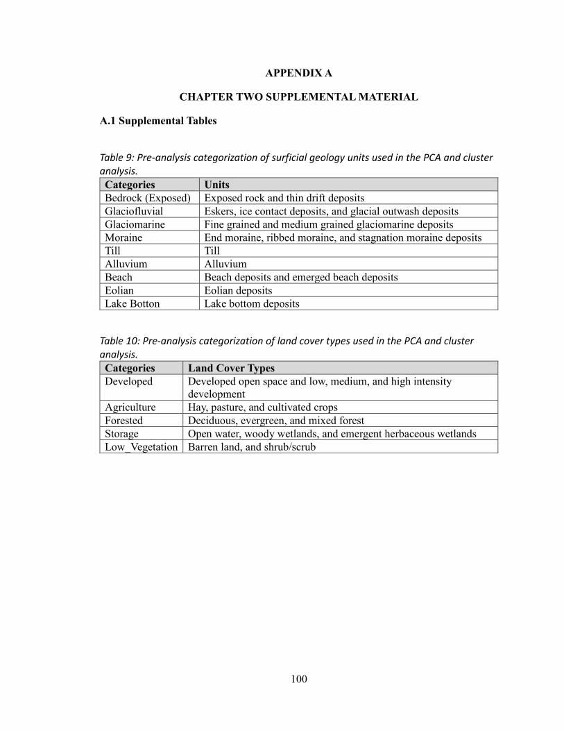
100
APPENDIX A
CHAPTER TWO SUPPLEMENTAL MATERIAL
A.1 Supplemental Tables
Table 9: Pre-analysis categorization of surficial geology units used in the PCA and cluster analysis. Categories Units Bedrock (Exposed) Exposed rock and thin drift deposits Glaciofluvial Eskers, ice contact deposits, and glacial outwash deposits Glaciomarine Fine grained and medium grained glaciomarine deposits Moraine End moraine, ribbed moraine, and stagnation moraine deposits Till Till Alluvium Alluvium Beach Beach deposits and emerged beach deposits Eolian Eolian deposits Lake Botton Lake bottom deposits
Table 10: Pre-analysis categorization of land cover types used in the PCA and cluster analysis. Categories Land Cover Types Developed Developed open space and low, medium, and high intensity
development Agriculture Hay, pasture, and cultivated crops Forested Deciduous, evergreen, and mixed forest Storage Open water, woody wetlands, and emergent herbaceous wetlands Low_Vegetation Barren land, and shrub/scrub
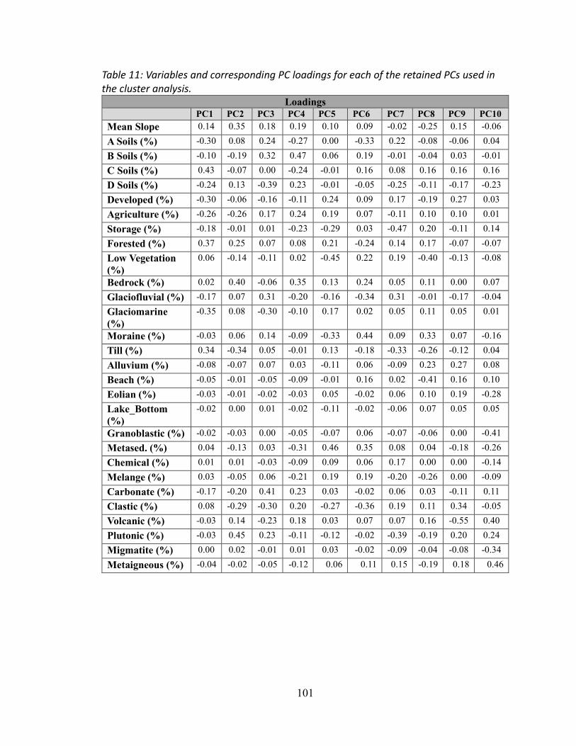
101
Table 11: Variables and corresponding PC loadings for each of the retained PCs used in the cluster analysis.
Loadings PC1 PC2 PC3 PC4 PC5 PC6 PC7 PC8 PC9 PC10 Mean Slope 0.14 0.35 0.18 0.19 0.10 0.09 -0.02 -0.25 0.15 -0.06 A Soils (%) -0.30 0.08 0.24 -0.27 0.00 -0.33 0.22 -0.08 -0.06 0.04 B Soils (%) -0.10 -0.19 0.32 0.47 0.06 0.19 -0.01 -0.04 0.03 -0.01 C Soils (%) 0.43 -0.07 0.00 -0.24 -0.01 0.16 0.08 0.16 0.16 0.16 D Soils (%) -0.24 0.13 -0.39 0.23 -0.01 -0.05 -0.25 -0.11 -0.17 -0.23 Developed (%) -0.30 -0.06 -0.16 -0.11 0.24 0.09 0.17 -0.19 0.27 0.03 Agriculture (%) -0.26 -0.26 0.17 0.24 0.19 0.07 -0.11 0.10 0.10 0.01 Storage (%) -0.18 -0.01 0.01 -0.23 -0.29 0.03 -0.47 0.20 -0.11 0.14 Forested (%) 0.37 0.25 0.07 0.08 0.21 -0.24 0.14 0.17 -0.07 -0.07 Low Vegetation (%)
0.06 -0.14 -0.11 0.02 -0.45 0.22 0.19 -0.40 -0.13 -0.08
Bedrock (%) 0.02 0.40 -0.06 0.35 0.13 0.24 0.05 0.11 0.00 0.07 Glaciofluvial (%) -0.17 0.07 0.31 -0.20 -0.16 -0.34 0.31 -0.01 -0.17 -0.04 Glaciomarine (%)
-0.35 0.08 -0.30 -0.10 0.17 0.02 0.05 0.11 0.05 0.01
Moraine (%) -0.03 0.06 0.14 -0.09 -0.33 0.44 0.09 0.33 0.07 -0.16 Till (%) 0.34 -0.34 0.05 -0.01 0.13 -0.18 -0.33 -0.26 -0.12 0.04 Alluvium (%) -0.08 -0.07 0.07 0.03 -0.11 0.06 -0.09 0.23 0.27 0.08 Beach (%) -0.05 -0.01 -0.05 -0.09 -0.01 0.16 0.02 -0.41 0.16 0.10 Eolian (%) -0.03 -0.01 -0.02 -0.03 0.05 -0.02 0.06 0.10 0.19 -0.28 Lake_Bottom (%)
-0.02 0.00 0.01 -0.02 -0.11 -0.02 -0.06 0.07 0.05 0.05
Granoblastic (%) -0.02 -0.03 0.00 -0.05 -0.07 0.06 -0.07 -0.06 0.00 -0.41 Metased. (%) 0.04 -0.13 0.03 -0.31 0.46 0.35 0.08 0.04 -0.18 -0.26 Chemical (%) 0.01 0.01 -0.03 -0.09 0.09 0.06 0.17 0.00 0.00 -0.14 Melange (%) 0.03 -0.05 0.06 -0.21 0.19 0.19 -0.20 -0.26 0.00 -0.09 Carbonate (%) -0.17 -0.20 0.41 0.23 0.03 -0.02 0.06 0.03 -0.11 0.11 Clastic (%) 0.08 -0.29 -0.30 0.20 -0.27 -0.36 0.19 0.11 0.34 -0.05 Volcanic (%) -0.03 0.14 -0.23 0.18 0.03 0.07 0.07 0.16 -0.55 0.40 Plutonic (%) -0.03 0.45 0.23 -0.11 -0.12 -0.02 -0.39 -0.19 0.20 0.24 Migmatite (%) 0.00 0.02 -0.01 0.01 0.03 -0.02 -0.09 -0.04 -0.08 -0.34 Metaigneous (%) -0.04 -0.02 -0.05 -0.12 0.06 0.11 0.15 -0.19 0.18 0.46
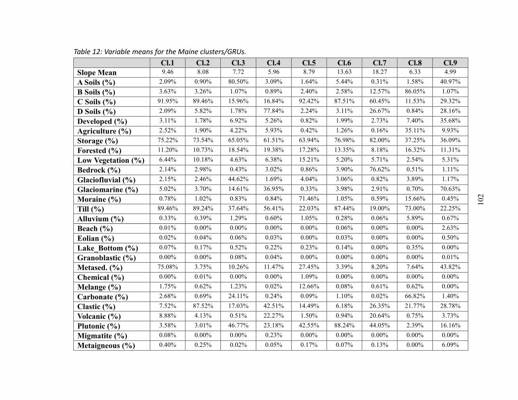
102
Table 12: Variable means for the Maine clusters/GRUs. Cl.1 Cl.2 Cl.3 Cl.4 Cl.5 Cl.6 Cl.7 Cl.8 Cl.9 Slope Mean 9.46 8.08 7.72 5.96 8.79 13.63 18.27 6.33 4.99
A Soils (%) 2.09% 0.90% 80.50% 3.09% 1.64% 5.44% 0.31% 1.58% 40.97%
B Soils (%) 3.63% 3.26% 1.07% 0.89% 2.40% 2.58% 12.57% 86.05% 1.07%
C Soils (%) 91.95% 89.46% 15.96% 16.84% 92.42% 87.51% 60.45% 11.53% 29.32%
D Soils (%) 2.09% 5.82% 1.78% 77.84% 2.24% 3.11% 26.67% 0.84% 28.16%
Developed (%) 3.11% 1.78% 6.92% 5.26% 0.82% 1.99% 2.73% 7.40% 35.68%
Agriculture (%) 2.52% 1.90% 4.22% 5.93% 0.42% 1.26% 0.16% 35.11% 9.93%
Storage (%) 75.22% 73.54% 65.05% 61.51% 63.94% 76.98% 82.00% 37.25% 36.09%
Forested (%) 11.20% 10.73% 18.54% 19.38% 17.28% 13.35% 8.18% 16.32% 11.31%
Low Vegetation (%) 6.44% 10.18% 4.63% 6.38% 15.21% 5.20% 5.71% 2.54% 5.31%
Bedrock (%) 2.14% 2.98% 0.43% 3.02% 0.86% 3.90% 76.62% 0.51% 1.11%
Glaciofluvial (%) 2.15% 2.46% 44.62% 1.69% 4.04% 3.06% 0.82% 3.89% 1.17%
Glaciomarine (%) 5.02% 3.70% 14.61% 36.95% 0.33% 3.98% 2.91% 0.70% 70.63%
Moraine (%) 0.78% 1.02% 0.83% 0.84% 71.46% 1.05% 0.59% 15.66% 0.45%
Till (%) 89.46% 89.24% 37.64% 56.41% 22.03% 87.44% 19.00% 73.00% 22.25%
Alluvium (%) 0.33% 0.39% 1.29% 0.60% 1.05% 0.28% 0.06% 5.89% 0.67%
Beach (%) 0.01% 0.00% 0.00% 0.00% 0.00% 0.06% 0.00% 0.00% 2.63%
Eolian (%) 0.02% 0.04% 0.06% 0.03% 0.00% 0.03% 0.00% 0.00% 0.50%
Lake_Bottom (%) 0.07% 0.17% 0.52% 0.22% 0.23% 0.14% 0.00% 0.35% 0.00%
Granoblastic (%) 0.00% 0.00% 0.08% 0.04% 0.00% 0.00% 0.00% 0.00% 0.01%
Metased. (%) 75.08% 3.75% 10.26% 11.47% 27.45% 3.39% 8.20% 7.64% 43.82%
Chemical (%) 0.00% 0.01% 0.00% 0.00% 1.09% 0.00% 0.00% 0.00% 0.00%
Melange (%) 1.75% 0.62% 1.23% 0.02% 12.66% 0.08% 0.61% 0.62% 0.00%
Carbonate (%) 2.68% 0.69% 24.11% 0.24% 0.09% 1.10% 0.02% 66.82% 1.40%
Clastic (%) 7.52% 87.52% 17.03% 42.51% 14.49% 6.18% 26.35% 21.77% 28.78%
Volcanic (%) 8.88% 4.13% 0.51% 22.27% 1.50% 0.94% 20.64% 0.75% 3.73%
Plutonic (%) 3.58% 3.01% 46.77% 23.18% 42.55% 88.24% 44.05% 2.39% 16.16%
Migmatite (%) 0.08% 0.00% 0.00% 0.23% 0.00% 0.00% 0.00% 0.00% 0.00%
Metaigneous (%) 0.40% 0.25% 0.02% 0.05% 0.17% 0.07% 0.13% 0.00% 6.09%

103
Table 13: Z-scored variable means for the Maine clusters/GRUs. Cl.1 Cl.2 Cl.3 Cl.4 Cl.5 Cl.6 Cl.7 Cl.8 Cl.9 Slope Mean 0.05 -0.28 -0.36 -0.78 -0.11 1.04 2.14 -0.69 -1.01
A Soils (%) -0.47 -0.52 2.36 -0.44 -0.49 -0.35 -0.54 -0.49 0.93
B Soils (%) -0.32 -0.34 -0.42 -0.42 -0.37 -0.36 0.00 2.64 -0.42
C Soils (%) 1.02 0.95 -1.08 -1.05 1.03 0.89 0.15 -1.20 -0.71
D Soils (%) -0.57 -0.42 -0.58 2.41 -0.56 -0.53 0.40 -0.62 0.46
Developed (%) -0.38 -0.51 -0.03 -0.19 -0.60 -0.49 -0.42 0.01 2.61
Agriculture (%) -0.39 -0.45 -0.24 -0.08 -0.58 -0.50 -0.60 2.56 0.28
Storage (%) 0.70 0.60 0.09 -0.12 0.03 0.81 1.11 -1.58 -1.65
Forested (%) -0.71 -0.83 1.14 1.35 0.82 -0.17 -1.48 0.58 -0.69
Low Vegetation (%) -0.11 0.89 -0.59 -0.13 2.24 -0.44 -0.30 -1.15 -0.41
Bedrock (%) -0.32 -0.29 -0.39 -0.29 -0.37 -0.25 2.66 -0.39 -0.36
Glaciofluvial (%) -0.35 -0.33 2.66 -0.38 -0.22 -0.29 -0.44 -0.23 -0.42
Glaciomarine (%) -0.44 -0.50 -0.03 0.91 -0.64 -0.48 -0.53 -0.62 2.33
Moraine (%) -0.41 -0.40 -0.40 -0.40 2.61 -0.39 -0.41 0.23 -0.42
Till (%) 1.12 1.11 -0.57 0.04 -1.08 1.05 -1.18 0.58 -1.08
Alluvium (%) -0.47 -0.43 0.06 -0.32 -0.07 -0.49 -0.61 2.61 -0.28
Beach (%) -0.33 -0.34 -0.34 -0.34 -0.34 -0.28 -0.34 -0.34 2.67
Eolian (%) -0.35 -0.22 -0.12 -0.26 -0.47 -0.29 -0.47 -0.47 2.65
Lake_Bottom (%) -0.70 -0.10 1.95 0.21 0.26 -0.29 -1.14 0.96 -1.14
Granoblastic (%) -0.52 -0.52 2.29 1.04 -0.52 -0.52 -0.52 -0.52 -0.19
Metased. (%) 2.24 -0.73 -0.46 -0.41 0.26 -0.74 -0.54 -0.56 0.94
Chemical (%) -0.34 -0.31 -0.34 -0.34 2.67 -0.33 -0.34 -0.34 -0.34
Melange (%) -0.05 -0.33 -0.18 -0.48 2.64 -0.46 -0.33 -0.33 -0.48
Carbonate (%) -0.36 -0.45 0.59 -0.47 -0.48 -0.43 -0.48 2.50 -0.42
Clastic (%) -0.82 2.38 -0.44 0.58 -0.54 -0.87 -0.07 -0.25 0.03
Volcanic (%) 0.21 -0.34 -0.76 1.77 -0.64 -0.71 1.58 -0.73 -0.39
Plutonic (%) -0.93 -0.95 0.59 -0.24 0.44 2.05 0.49 -0.97 -0.49
Migmatite (%) 0.58 -0.45 -0.45 2.51 -0.45 -0.41 -0.45 -0.45 -0.45
Metaigneous (%) -0.20 -0.28 -0.39 -0.38 -0.31 -0.37 -0.34 -0.40 2.66
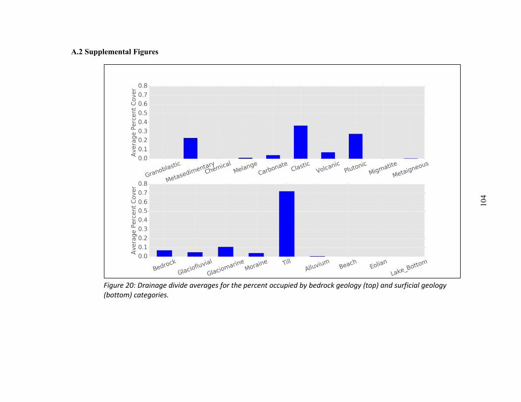
104
A.2 Supplemental Figures
Figure 20: Drainage divide averages for the percent occupied by bedrock geology (top) and surficial geology (bottom) categories.
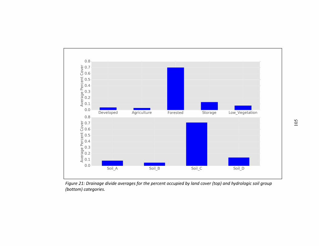
105
Figure 21: Drainage divide averages for the percent occupied by land cover (top) and hydrologic soil group (bottom) categories.
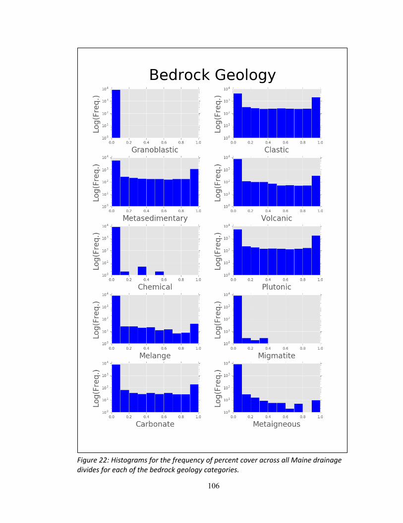
106
Figure 22: Histograms for the frequency of percent cover across all Maine drainage divides for each of the bedrock geology categories.
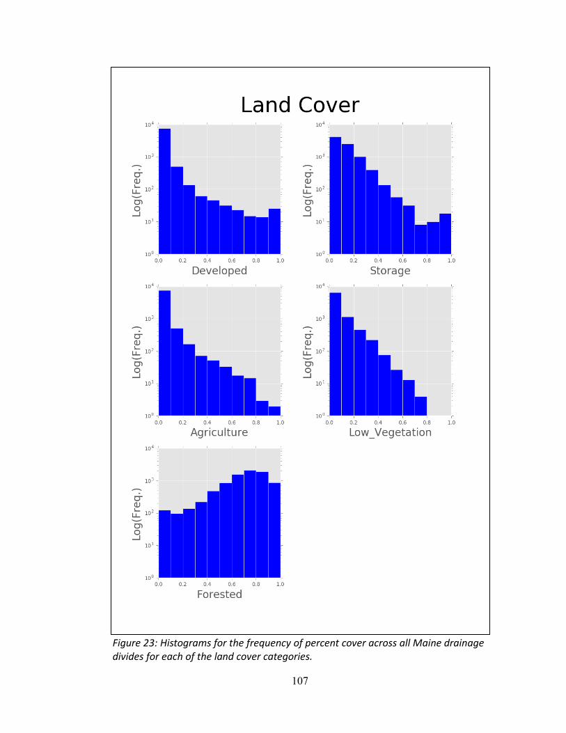
107
Figure 23: Histograms for the frequency of percent cover across all Maine drainage divides for each of the land cover categories.
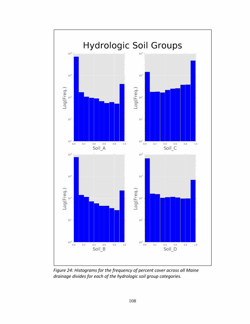
108
Figure 24: Histograms for the frequency of percent cover across all Maine drainage divides for each of the hydrologic soil group categories.

109
Figure 25: Histograms for the frequency of percent cover across all Maine drainage divides for each of the surficial geology categories.

110
Figure 26: Maine GRUs derived from PCA and cluster analysis.
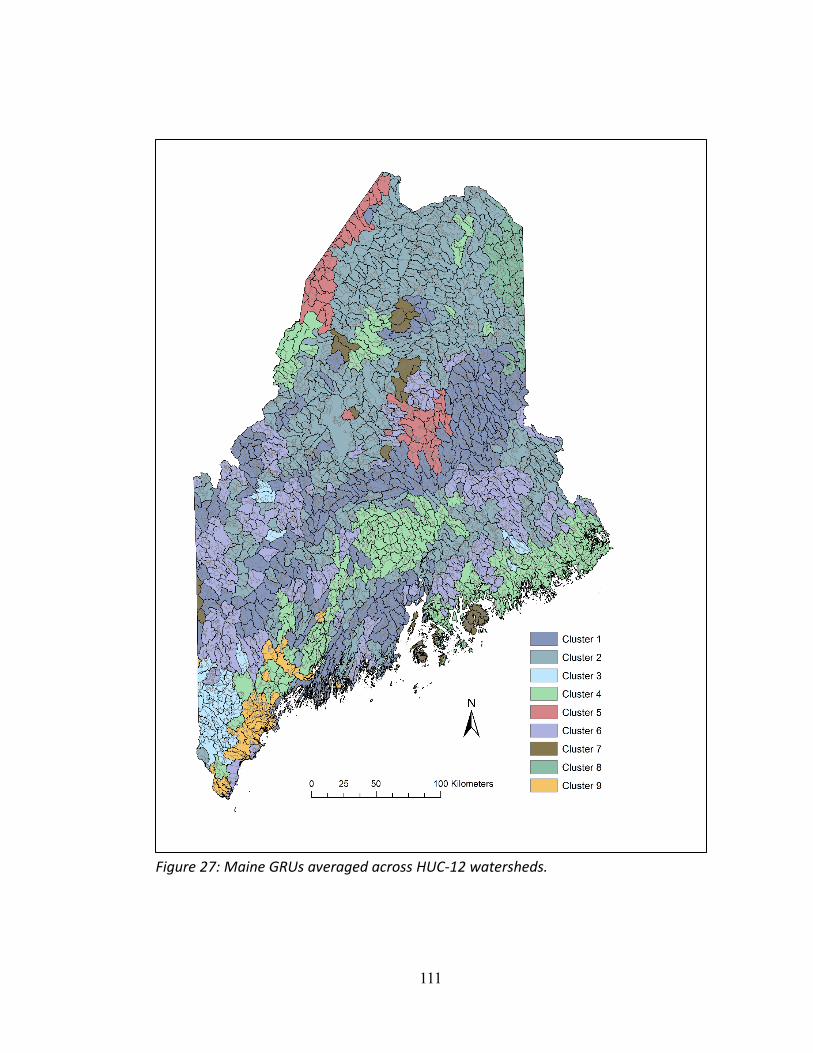
111
Figure 27: Maine GRUs averaged across HUC-12 watersheds.
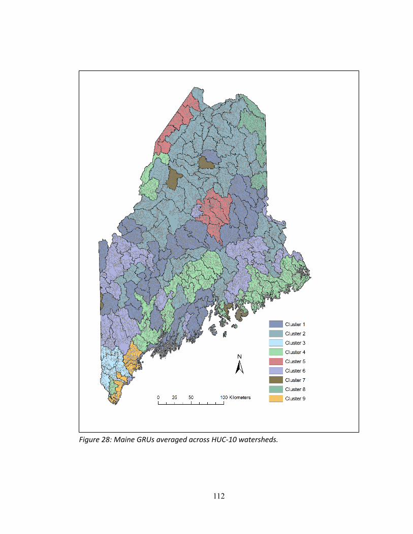
112
Figure 28: Maine GRUs averaged across HUC-10 watersheds.
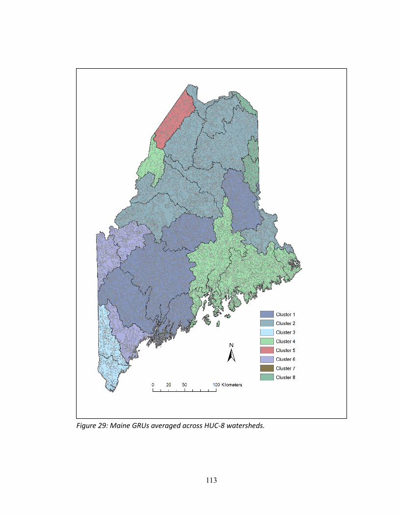
113
Figure 29: Maine GRUs averaged across HUC-8 watersheds.

114
Figure 30-A: Sensitivity function plots for selected USGS monitoring stations. The x-axis is drainage area normalized discharge during periods of receding flows. The y-axis represents the rate (slope) of flow decrease at each instance.

115
Figure 30-B: Sensitivity function plots for selected USGS monitoring stations. The x-axis is drainage area normalized discharge during periods of receding flows. The y-axis represents the rate (slope) of flow decrease at each instance.
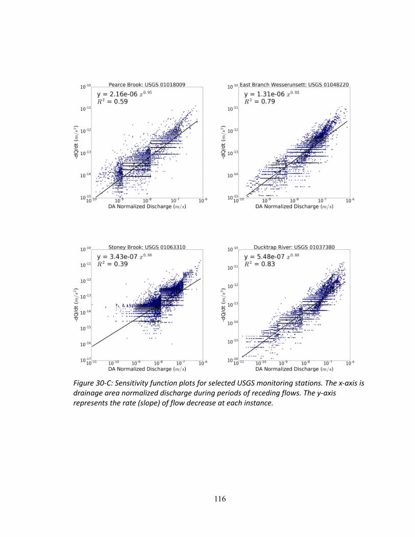
116
Figure 30-C: Sensitivity function plots for selected USGS monitoring stations. The x-axis is drainage area normalized discharge during periods of receding flows. The y-axis represents the rate (slope) of flow decrease at each instance.
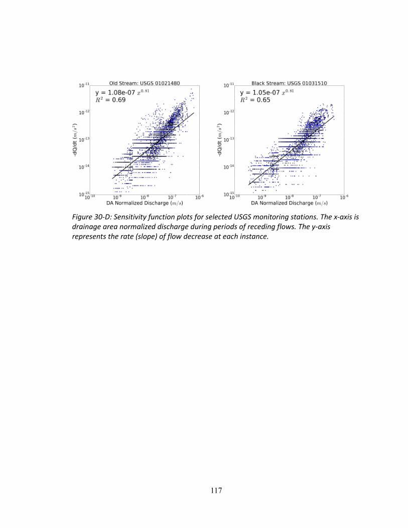
117
Figure 30-D: Sensitivity function plots for selected USGS monitoring stations. The x-axis is drainage area normalized discharge during periods of receding flows. The y-axis represents the rate (slope) of flow decrease at each instance.
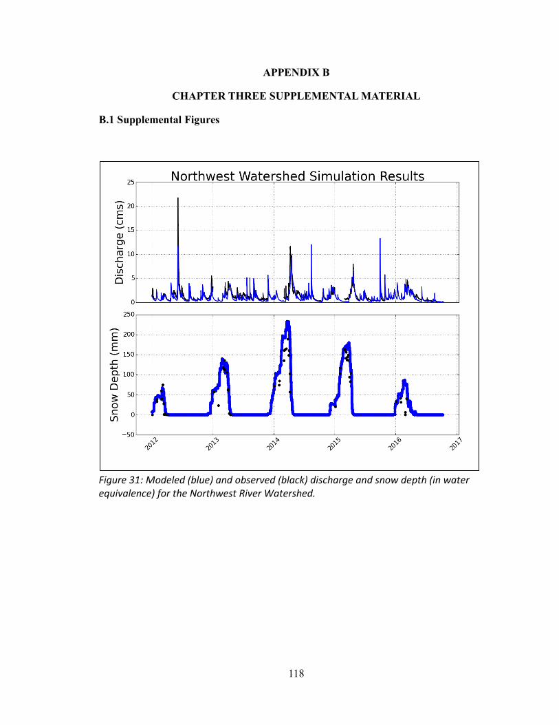
118
APPENDIX B
CHAPTER THREE SUPPLEMENTAL MATERIAL
B.1 Supplemental Figures
Figure 31: Modeled (blue) and observed (black) discharge and snow depth (in water equivalence) for the Northwest River Watershed.

119
Figure 32: Modeled (blue) and observed (black) discharge and snow depth (in water equivalence) for the Webhannet River Watershed.
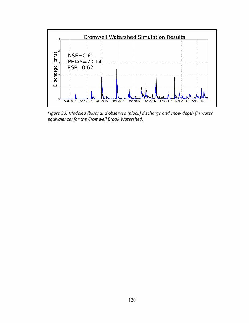
120
Figure 33: Modeled (blue) and observed (black) discharge and snow depth (in water equivalence) for the Cromwell Brook Watershed.

121
Figure 34: Observed precipitation (gray) and temperature (black) measured in Augusta, ME. The range of modifications to these variables for climate scenarios based on CMIP5 data are plotted in red (temperature) and blue (precipitation).

122
Figure 35: Flow duration curves for the Northwest River, the Webhannet River, and Cromwell Brook under the five scenario conditions compared to current climate conditions.
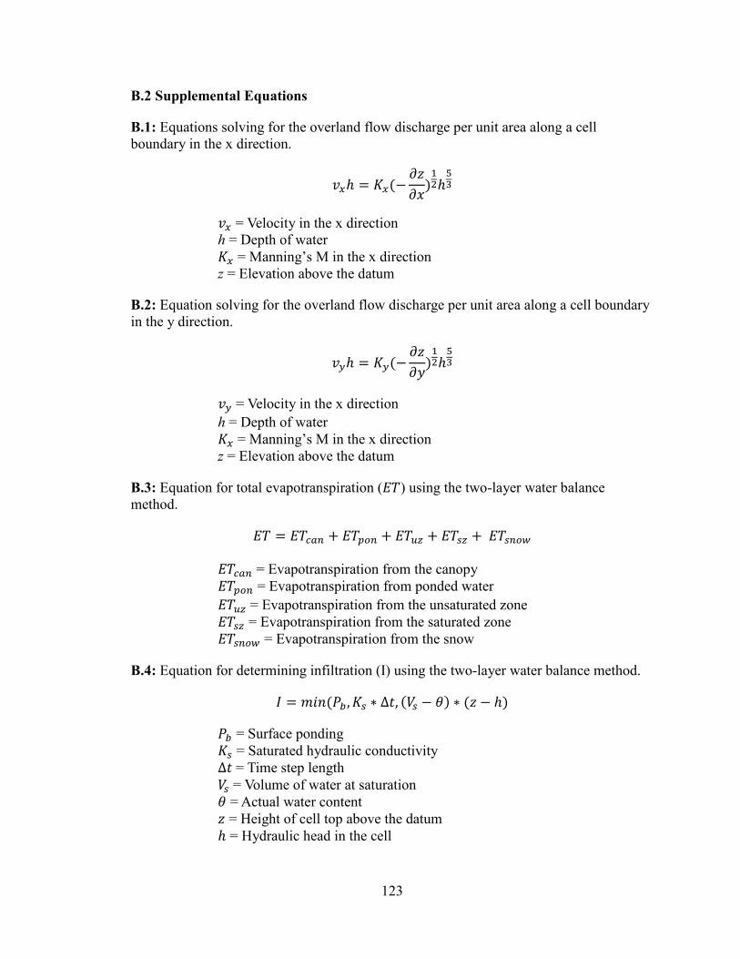
123
B.2 Supplemental Equations
B.1: Equations solving for the overland flow discharge per unit area along a cell boundary in the x direction.
𝑣𝑣𝑥𝑥ℎ = 𝐾𝐾𝑥𝑥(−𝜕𝜕𝜕𝜕𝜕𝜕𝜕𝜕
)12ℎ
53
𝑣𝑣𝑥𝑥 = Velocity in the x direction h = Depth of water 𝐾𝐾𝑥𝑥 = Manning’s M in the x direction z = Elevation above the datum
B.2: Equation solving for the overland flow discharge per unit area along a cell boundary in the y direction.
𝑣𝑣𝑦𝑦ℎ = 𝐾𝐾𝑦𝑦(−𝜕𝜕𝜕𝜕𝜕𝜕𝜕𝜕
)12ℎ
53
𝑣𝑣𝑦𝑦 = Velocity in the x direction h = Depth of water 𝐾𝐾𝑥𝑥 = Manning’s M in the x direction z = Elevation above the datum
B.3: Equation for total evapotranspiration (𝐸𝐸𝑇𝑇) using the two-layer water balance method.
𝐸𝐸𝑇𝑇 = 𝐸𝐸𝑇𝑇𝑐𝑐𝑐𝑐𝑛𝑛 + 𝐸𝐸𝑇𝑇𝑝𝑝𝑝𝑝𝑛𝑛 + 𝐸𝐸𝑇𝑇𝑢𝑢𝑢𝑢 + 𝐸𝐸𝑇𝑇𝑠𝑠𝑢𝑢 + 𝐸𝐸𝑇𝑇𝑠𝑠𝑛𝑛𝑝𝑝𝑠𝑠
𝐸𝐸𝑇𝑇𝑐𝑐𝑐𝑐𝑛𝑛 = Evapotranspiration from the canopy 𝐸𝐸𝑇𝑇𝑝𝑝𝑝𝑝𝑛𝑛 = Evapotranspiration from ponded water 𝐸𝐸𝑇𝑇𝑢𝑢𝑢𝑢 = Evapotranspiration from the unsaturated zone 𝐸𝐸𝑇𝑇𝑠𝑠𝑢𝑢 = Evapotranspiration from the saturated zone 𝐸𝐸𝑇𝑇𝑠𝑠𝑛𝑛𝑝𝑝𝑠𝑠 = Evapotranspiration from the snow
B.4: Equation for determining infiltration (I) using the two-layer water balance method.
𝑃𝑃 = 𝑚𝑚𝑚𝑚𝑚𝑚 (𝑃𝑃𝑏𝑏 ,𝐾𝐾𝑠𝑠 ∗ ∆𝑑𝑑, (𝑉𝑉𝑠𝑠 − 𝜃𝜃) ∗ (𝜕𝜕 − ℎ)
𝑃𝑃𝑏𝑏 = Surface ponding 𝐾𝐾𝑠𝑠 = Saturated hydraulic conductivity ∆𝑑𝑑 = Time step length 𝑉𝑉𝑠𝑠 = Volume of water at saturation 𝜃𝜃 = Actual water content 𝜕𝜕 = Height of cell top above the datum ℎ = Hydraulic head in the cell

124
B.5: Linear reservoir method equation for the storage of a reservoir (W).
𝑑𝑑 = 𝑘𝑘 ∗ 𝑄𝑄
𝑘𝑘 = Storage constant 𝑄𝑄 = Discharge outputs (i.e. interflow and baseflow)
B.6: The vertically integrated equation of the conservation of mass.
𝜕𝜕𝑄𝑄𝜕𝜕𝜕𝜕
+𝜕𝜕𝐷𝐷𝜕𝜕𝑑𝑑
= 𝑞𝑞
Q = Discharge A = Flow area t = Time q = Later inflows
B.7: The vertically integrated equation of the conservation of momentum.
𝜕𝜕𝑄𝑄𝜕𝜕𝑑𝑑
+𝜕𝜕(∝ 𝑄𝑄2
𝐷𝐷 )𝜕𝜕𝜕𝜕
+ 𝑔𝑔𝐷𝐷𝜕𝜕ℎ𝜕𝜕𝜕𝜕
+𝑔𝑔𝑄𝑄|𝑄𝑄|𝑃𝑃2𝐷𝐷𝑅𝑅
= 0
Q = Discharge A = Flow area t = Time q = Later inflows C = Chezy’s resistance coefficient R = Hydraulic radius g = Acceleration due to gravity ∝ = Momentum distribution coefficient
B.8: Equation for temperature melting of snow (𝑀𝑀𝐸𝐸).
𝑀𝑀𝐸𝐸 = 𝐽𝐽𝐸𝐸(𝑇𝑇 − 𝑇𝑇0)
𝐽𝐽𝐸𝐸 = Degree-day factor for snow melt T = Air temperature 𝑇𝑇0 = Freezing temperature of snow
B.9: Equation for radiation melting of snow (𝑀𝑀𝑅𝑅).
𝑀𝑀𝑅𝑅 = −𝐽𝐽𝑅𝑅𝑐𝑐𝑑𝑑𝑅𝑅𝑠𝑠𝑠𝑠
𝐽𝐽𝑅𝑅𝑐𝑐𝑑𝑑 = Radiation melting factor for snow melt 𝑅𝑅𝑠𝑠𝑠𝑠 = Incoming solar radiation
125
B.10: Equation for energy melting of snow (𝑀𝑀𝐸𝐸).
𝑀𝑀𝐸𝐸 = 𝐽𝐽𝐸𝐸𝑃𝑃(𝑇𝑇 − 𝑇𝑇0)
𝐽𝐽𝐸𝐸 = Energy snow melting coefficient for the energy of liquid rain P = Precipitation T = Air temperature 𝑇𝑇0 = Freezing temperature of snow

126
APPENDIX C
CHAPTER FOUR SUPPLEMENTAL MATERIAL
C.1 Supplemental Figures
Figure 36: Box and whisker plot of bankfull area vs channel order.

127
BIOGRAPHY OF THE AUTHOR
Brett Gerard was born in Lafayette, Louisiana. He is the son of Brian and Terrell Gerard.
Brett graduated of The Woodlands High School (2005) and Texas State University (B.S.
in 2010; M.S. in 2012). He began pursuit of a Ph.D. at the University of Maine in January
2013.
In 2004 he met the woman that in now his wife, Adele Gerard. On November 29, 2016
they welcomed Braxton Raymond Gerard into their family.
He is a candidate for a Doctor of Philosophy degree in Earth and Climate Science from
the University of Maine in December 2018.