stream processing in the cloud
TRANSCRIPT
Imperial College of Science, Technology and Medicine
Department of Computing
Stream Processing in the Cloud
Wilhelm Kleiminger
Submitted in part fulfilment of the requirements for theMEng Honours degree in Computing of Imperial College, June 2010
1

2
Abstract
Stock exchanges, sensor networks and other publish/subscribe systems need to deal with high-volume streams of real-time data. Especially financial data has to be processed with low latencyin order to cater for high-frequency trading algorithms. In order to deal with the large amountsof incoming data, the stream processing task has to be distributed. Traditionally, distributedstream processing systems balanced their load over a static number of nodes using operatorplacement or pipelining.
In this report we propose a novel way of doing stream processing by exploiting scalable clusterarchitectures as provided by IaaS/cloud solutions such as Amazon’s EC2. We show how toimplement a cloud-centric stream processor based on the MapReduce framework. We will thendesign a load balancing algorithm which allows a local stream processor to request additionalresources from the cloud when its capacity to handle the input stream becomes insufficient .
i

ii
Acknowledgements
I would like to thank:
• My supervisor Peter Pietzuch for the project proposal and his great support and encour-agement throughout the project.
• My second supervisor Alexander Wolf for the insightful discussions on MapReduce.
• Eva Kalyvianaki for her help throughout the project and all the great suggestions leadingto this report.
• Nicholas Ng, for proof-reading the script and coming up with the ingenious acronymM.A.P.S. for the custom Python MapReduce implementation. M.A.P.S. stands for “MyAwesome Python Script”.
• My sister Lisa for proof-reading and my parents Elke and Jurgen for their great supportthroughout school and university. Vielen Dank!
iii

iv
Contents
Abstract i
Acknowledgements iii
1 Introduction 1
1.1 Contributions . . . . . . . . . . . . . . . . . . . . . . . . . . . . . . . . . . . . . . 3
1.2 Outline of this report . . . . . . . . . . . . . . . . . . . . . . . . . . . . . . . . . . 3
2 Background 5
2.1 Financial Algorithms . . . . . . . . . . . . . . . . . . . . . . . . . . . . . . . . . . 5
2.1.1 Foundations . . . . . . . . . . . . . . . . . . . . . . . . . . . . . . . . . . . 6
2.1.2 Put and call options . . . . . . . . . . . . . . . . . . . . . . . . . . . . . . 6
2.1.3 Arbitrage opportunities . . . . . . . . . . . . . . . . . . . . . . . . . . . . 7
2.2 Cloud computing . . . . . . . . . . . . . . . . . . . . . . . . . . . . . . . . . . . . 8
2.2.1 MapReduce . . . . . . . . . . . . . . . . . . . . . . . . . . . . . . . . . . . 8
2.2.2 Sawzall . . . . . . . . . . . . . . . . . . . . . . . . . . . . . . . . . . . . . 10
2.2.3 Hadoop . . . . . . . . . . . . . . . . . . . . . . . . . . . . . . . . . . . . . 11
2.2.4 Remote Procedure Calls . . . . . . . . . . . . . . . . . . . . . . . . . . . . 12
2.2.5 Amazon EC2 . . . . . . . . . . . . . . . . . . . . . . . . . . . . . . . . . . 13
2.3 Stream processing . . . . . . . . . . . . . . . . . . . . . . . . . . . . . . . . . . . 14
2.3.1 Mortar . . . . . . . . . . . . . . . . . . . . . . . . . . . . . . . . . . . . . . 14
2.3.2 STREAM . . . . . . . . . . . . . . . . . . . . . . . . . . . . . . . . . . . . 15
2.3.3 Cayuga . . . . . . . . . . . . . . . . . . . . . . . . . . . . . . . . . . . . . 16
2.3.4 MapReduce Online . . . . . . . . . . . . . . . . . . . . . . . . . . . . . . . 18
2.4 Load balancing . . . . . . . . . . . . . . . . . . . . . . . . . . . . . . . . . . . . . 19
v
vi CONTENTS
2.4.1 Load-balancing in distributed web-servers . . . . . . . . . . . . . . . . . . 19
2.4.2 Locally aware request distribution . . . . . . . . . . . . . . . . . . . . . . 20
2.4.3 TCP Splicing . . . . . . . . . . . . . . . . . . . . . . . . . . . . . . . . . . 21
2.5 Summary . . . . . . . . . . . . . . . . . . . . . . . . . . . . . . . . . . . . . . . . 21
3 Stream Processing With Hadoop 23
3.1 From batch to stream processing . . . . . . . . . . . . . . . . . . . . . . . . . . . 23
3.2 Network I/O . . . . . . . . . . . . . . . . . . . . . . . . . . . . . . . . . . . . . . 24
3.2.1 Implementation of the changes . . . . . . . . . . . . . . . . . . . . . . . . 25
3.3 Persistent queries . . . . . . . . . . . . . . . . . . . . . . . . . . . . . . . . . . . . 27
3.3.1 Restarting jobs . . . . . . . . . . . . . . . . . . . . . . . . . . . . . . . . . 28
3.3.2 Optimisation attempts . . . . . . . . . . . . . . . . . . . . . . . . . . . . . 28
3.3.3 Hadoop overhead problems . . . . . . . . . . . . . . . . . . . . . . . . . . 29
3.4 Lessons learnt . . . . . . . . . . . . . . . . . . . . . . . . . . . . . . . . . . . . . . 31
4 MAPS: An Alternative Streaming MapReduce Framework 33
4.1 Motivation for Python as implementation language . . . . . . . . . . . . . . . . . 34
4.2 Design decisions . . . . . . . . . . . . . . . . . . . . . . . . . . . . . . . . . . . . 34
4.2.1 Role of the JobTracker . . . . . . . . . . . . . . . . . . . . . . . . . . . . . 35
4.2.2 Role of the TaskTrackers . . . . . . . . . . . . . . . . . . . . . . . . . . . 36
4.2.3 Possible extensions . . . . . . . . . . . . . . . . . . . . . . . . . . . . . . . 36
4.3 Components to be implemented . . . . . . . . . . . . . . . . . . . . . . . . . . . . 36
4.3.1 Master node . . . . . . . . . . . . . . . . . . . . . . . . . . . . . . . . . . 37
4.3.2 Slave nodes . . . . . . . . . . . . . . . . . . . . . . . . . . . . . . . . . . . 38
4.4 Implementation . . . . . . . . . . . . . . . . . . . . . . . . . . . . . . . . . . . . . 38
4.4.1 Helper threads . . . . . . . . . . . . . . . . . . . . . . . . . . . . . . . . . 38
4.4.2 Inter-node communication - Python Remote Objects . . . . . . . . . . . . 38
4.4.3 Dynamic loading of modules . . . . . . . . . . . . . . . . . . . . . . . . . 39
4.4.4 Query validation . . . . . . . . . . . . . . . . . . . . . . . . . . . . . . . . 40
4.5 Discussion . . . . . . . . . . . . . . . . . . . . . . . . . . . . . . . . . . . . . . . . 41
CONTENTS vii
5 Load Balancing Into The Cloud 43
5.1 Local stream processor . . . . . . . . . . . . . . . . . . . . . . . . . . . . . . . . . 43
5.1.1 Simplifications . . . . . . . . . . . . . . . . . . . . . . . . . . . . . . . . . 44
5.1.2 Query invocation . . . . . . . . . . . . . . . . . . . . . . . . . . . . . . . . 44
5.2 Design . . . . . . . . . . . . . . . . . . . . . . . . . . . . . . . . . . . . . . . . . . 44
5.2.1 Always-on load balancing . . . . . . . . . . . . . . . . . . . . . . . . . . . 45
5.2.2 Adaptive load balancing . . . . . . . . . . . . . . . . . . . . . . . . . . . . 46
5.3 Implementation . . . . . . . . . . . . . . . . . . . . . . . . . . . . . . . . . . . . . 50
5.3.1 Concurrent data structures . . . . . . . . . . . . . . . . . . . . . . . . . . 50
5.3.2 Logging . . . . . . . . . . . . . . . . . . . . . . . . . . . . . . . . . . . . . 50
5.3.3 Components to be implemented . . . . . . . . . . . . . . . . . . . . . . . . 50
5.4 Discussion . . . . . . . . . . . . . . . . . . . . . . . . . . . . . . . . . . . . . . . . 53
6 Evaluation 55
6.1 Stream processing in the cloud . . . . . . . . . . . . . . . . . . . . . . . . . . . . 56
6.1.1 The Put/Call parity problem . . . . . . . . . . . . . . . . . . . . . . . . . 56
6.1.2 Theoretical analysis of the parallel algorithm . . . . . . . . . . . . . . . . 57
6.1.3 Hadoop vs Python MapReduce . . . . . . . . . . . . . . . . . . . . . . . . 59
6.1.4 Conclusion . . . . . . . . . . . . . . . . . . . . . . . . . . . . . . . . . . . 63
6.2 Loadbalancing into the cloud . . . . . . . . . . . . . . . . . . . . . . . . . . . . . 64
6.2.1 Experimental setup . . . . . . . . . . . . . . . . . . . . . . . . . . . . . . . 64
6.2.2 Analysis of the data set . . . . . . . . . . . . . . . . . . . . . . . . . . . . 64
6.2.3 Input parameters . . . . . . . . . . . . . . . . . . . . . . . . . . . . . . . . 65
6.2.4 Measured properties . . . . . . . . . . . . . . . . . . . . . . . . . . . . . . 66
6.2.5 Always-on: Finding the best split . . . . . . . . . . . . . . . . . . . . . . . 66
6.2.6 Adaptive load balancing . . . . . . . . . . . . . . . . . . . . . . . . . . . . 67
6.2.7 Conclusion . . . . . . . . . . . . . . . . . . . . . . . . . . . . . . . . . . . 72
7 Conclusion 75
7.1 Project review . . . . . . . . . . . . . . . . . . . . . . . . . . . . . . . . . . . . . 75
7.1.1 Contributions . . . . . . . . . . . . . . . . . . . . . . . . . . . . . . . . . . 75
7.2 Future work . . . . . . . . . . . . . . . . . . . . . . . . . . . . . . . . . . . . . . . 76
viii CONTENTS
7.2.1 Improving the efficiency of the MapReduce framework . . . . . . . . . . . 76
7.2.2 Pipelined MapReduce jobs . . . . . . . . . . . . . . . . . . . . . . . . . . 76
7.2.3 MAPS scaling . . . . . . . . . . . . . . . . . . . . . . . . . . . . . . . . . . 76
7.2.4 Adapting Cayuga to scale on a cloud infrastructure . . . . . . . . . . . . . 77
7.2.5 Eliminating communication bottlenecks . . . . . . . . . . . . . . . . . . . 77
7.2.6 Parallel programming with language support - F# . . . . . . . . . . . . . 77
7.2.7 Cost-benefit analysis . . . . . . . . . . . . . . . . . . . . . . . . . . . . . . 77
Bibliography 78
Chapter 1
Introduction
Today’s information processing systems face formidable challenges as they are presented withnew data at ever-increasing rates [19]. In response, processing architectures have changed witha new emphasis on parallel architectures at the on-chip level. However, research has shownthat an increase in the number of cores cannot be seen as a panacea. As cores increase innumber and speed, communication becomes increasingly a bottleneck [4]. Alternative solutionslike clusters are still preferred for high performance applications. So while the traditional PChas seen advances in multi-core architectures, much of this effort is complemented by a movefrom local to cloud processing. Cloud-based computing seeks to address the issue that while inmost cases today’s computational resources are idling, they may still not be adequate in peakload situations. By sharing resources and requesting more power when needed, we can overcomethese bottlenecks. The result should improve both latency and reduce the cost to the user. Thisprojects seeks to evaluate a novel way of load balancing data intensive stream processing queriesinto a scalable cluster. The goal is to exploit the scalability of a cloud environment in order dealwith peaks in the input stream.
Cloud computing has certainly been one of the most hyped trends of the last few years. Theresult is that companies of tacked this name to a variety of different service offerings. Thismakes it difficult to come up with a single, concise definition. Kunze and Baun [27] have deriveda good definition from Ian Foster’s definition of grid computing [24]:
Cloud computing uses virtualised processing and storage resources in conjunctionwith modern web-technologies to deliver abstract, scalable platforms and applicationsas ondemand services. The billing of these services is directly tied to usage statistics.
We can distinguish between three applications of Cloud Computing: Infrastructure as a service(IaaS), Platform as a service (PaaS) and Software as a service (SaaS) [27]. IaaS describes aservice that offers computational resources for distributed applications. The infrastructure isflexible enough for the user to run his own operating system and applications. The adminis-tration of the system lies mostly with the user. PaaS takes some of the administration awayfrom the user and allows some (limited) programming of the resources. An example for this isGoogle’s App Engine. Finally, and probably most exposed to the general public are SaaS appli-cations. These are offerings such as Apples MobileMe and Google’s email and text processingapplications. They offer little to no customisation but the convenience of storing data off-site.We are interested in applying IaaS services to the computation of financial algorithms.
Recent years have seen a massive increase in algorithmic trading. Billions of pounds are traded bysoftware [40]. More than a quarter of all equity trades at Wall Street come down to algorithms
1
2 Chapter 1. Introduction
with little to no human intervention [21]. Financial markets emit hundreds of thousands ofmessages per second [31]. The exchanges have responded to the demand. The delay betweenthe time a trade is placed and filed at the Singapoore exchange for example has dropped toaround 15 milliseconds and other exchanges are following suit [33]. An algorithmic tradingsystems must therefore process real time data streams with very low latency to in order to staycompetitive. The arms-race over ever faster responses to changing market conditions necessitateshighly scalable stream processing systems.
Stream processing systems are fundamentally different to ordinary data processing systems.Streams are often too large, too numerous or the important events too sparse [29]. This meansdata has to be processed on the fly by pre-installed queries. In most cases only a small numberof tuples is interesting to the trader. The job of a stream processing system is to find these andmake them available in a manner similar to traditional publish/subscribe systems.
A number of systems have emerged to deal with these problems. The distributed systems com-munity coined the term Complex Event Stream Processing for evaluating the output of sensornetworks. A similar approach taken by database vendors such as Oracle is simply called EventStream Processing. The difference between the two is that the former advocates a publish/-subscribe approach [20], whereas the database vendors promote SQL and distributed databases.Current systems distribute the query over a number of nodes [13], thus focussing on the com-plexity of the query itself. We feel that these techniques are too rigid to dynamically scale ina cloud environment. Instead we have chosen to extend the MapReduce paradigm to enablestreaming queries.
MapReduce is based on ideas from functional programming. Two functions, map and reducetake over the task of implementing the query. This technology has been successfully employedby Google [19] and others [10] [25] [35] and is supported in by various IaaS providers [5] [6] [7].As MapReduce has orginally been designed for batch-processing, it will have to undergo somechanges to be applied to stream processing. Recently, a first step towards streaming MapReducehas been made with the Hadoop Online Prototype (HOP) [18]. We will build on this work toshow how a MapReduce stream processor can be implemented.
The choice to use the MapReduce framework is motivitated by our goal to provide efficient loadbalancing into the cloud. As we will show later in this report, the data rate of a stream islikely to vary a lot. From our data set, we found the highest demand on the stream processoroccurs in the morning, presumably as many trades are carried over from the previous day. Thewhole trading session lasts 6.5 hours. This is only just over a quarter of a day. Most tradingis done on work days. To provide resources 24/7 would not be economical [16]. Instead weopt to design a load balancing algorithm which dynamically responds to bursts in the inputstream and relieves the strain on a small-scale, local stream processor by out-sourcing some ofthe computation to the cloud. The MapReduce implementation on the cloud should then scaleas more computational power is required.
1.1. Contributions 3
1.1 Contributions
In this report we seek to complement the current state of the art in stream processing techniqueswith the following contributions:
1. Streaming extension for the Hadoop framework We will design and implement thenetwork components necessary to run a streaming MapReduce query on top of the Hadoopframework.
2. MAPS: A Lightweight MapReduce framework written in Python. Starting fromthe origins of MapReduce in functional programming, we describe the design and imple-mentation of a simple MapReduce stream processor written in Python. The design drawsfrom the lessons learned while working on the Hadoop framework.
3. Loadbalancing strategies to use the cloud in an existing stream processing setup. Weshow the design and implementation of a minimal version of a single node MapReducestream processor and how its resources can be complimented by our cloud implementationwith two load balancing strategies.
(a) Always-on approach: The cloud’s resources are always used to complement the localstream processor.
(b) Adaptive approach: The cloud’s resources are used on-demand to assisst the localstream processor.
4. We will evaluate the benefits and limitations of MapReduce for stream processingapplications. We will compare our two cloud-based stream processing solutions. Takingthe results into account, we will conclude by evaluating our loadbalancing techniques withrespect to their ability to assist a local stream processor.
1.2 Outline of this report
In Chapter 2 we will look at existing stream processing solutions, cover the background for ourMapReduce implementation and discuss some existing load balancing strategies. We will finishwith a short introduction to the financial concepts behind our streaming queries. Having laidthe theoretical foundations, Chapter 3 shows how the HOP/Hadoop framework can be extendedto process streaming queries. Building on the experiences from the Hadoop stream processor,Chapter 4 focuses on the design and implementation of a custom prototype for a MapReducestream processor. With a cloud-based solution in place, Chapter 5 focuses on the design ofsuitable load-balancing algorithms. In Chapter 6, we will evaluate the MapReduce paradigm inthe context of financial queries. We will conclude this report by looking at the performance ofthe load balancing algorithms designed in Chapter 5.

4 Chapter 1. Introduction
Chapter 2
Background
The goal of this project is to enable stream processing in the cloud by using a scalable MapReduceframework. In addition, we are going to evaluate a load balancing algorithm which allows usto utilise the resources of an IaaS provider on-demand. For the purpose of implementation andevaluation we will use a set of local nodes in the college’s datacentre. However, since this is ahomogeneous cluster, the results should be easily transferable to a real IaaS service. In order tointroduce this ultimate goal of running the MapReduce stream processor with an IaaS provider,we introduce Amazon’s EC2 offering in §2.2.5.
We will start this chapter with a short detour into finance to gain an insight into possible areasof applications of a stream processor and to explain the reasoning behind Put/Call parities -our chosen test query.
After this, we will formally introduce the MapReduce algorithm as designed by Google [19]. TheMapReduce algorithm enables data processing on a large number of off-the-shelf nodes. Thismeans that it has now become a focal point of any discussion on cloud computing in general. Wewill discuss its limitations and why we have initially chosen one of its variations (see §2.3.4) tobe part of our implementation. We will then introduce Sawzall, an effort by Google to create adomain specific language for MapReduce and proceed to Hadoop, an open-source implementationof the MapReduce framework. After having laid the algorithmic foundations, we will discussthe underlying infrastructure. Having covered the basics of MapReduce and the underlyingplatforms, we will concentrate on the current state of the art in stream processing systems anddiscuss why we have chosen to follow the rather novel path of utilising the MapReduce paradigm.We will conclude this chapter by looking at techniques currently employed in load-balancing andexplain how these are applicable to our problem.
2.1 Financial Algorithms
As laid out in the introduction, the financial services industry constitutes a major area ofapplication for stream processing. In our tests we are planning to use stream processing in thecloud to compute financial equations. We have a set of financial data available. This set containsthe quotes for options at various stock exchanges for a single day. In order to formulate a sensiblequery, we must understand the rationale behind the financial data given. In the following we willdiscuss the concepts behind put and call options as well as the concept of futures trading. At themoment, we are aiming to deploy a single query over the MapReduce network. We must thusformulate a query which makes sense both under the MapReduce as well as financial paradigms.
5
6 Chapter 2. Background
2.1.1 Foundations
Options An options contract can be described as follows. Farmer Enno sells investor Antjethe right to buy next year’s harvest at a specific strike price. Obviously, neither knows theactual value of the harvest. Enno produces biofuel. Now say the economy dips into recessionthe following year and substitute goods such as oil become cheaper. Then Enno’s biofuel willdrop in price as well and Antje is going to drop her option. She has lost the commission andany other associated fees. However, if the economy is well and Enno has an exceptional harvest,Antje will exercise her option. The price of the option is below the actual market price. Antjewill be able to sell the fuel at a premium.
Futures In contrast to options, futures are binding contracts over the purchase of a good.If Antje buys a futures contract on Enno’s harvest, she is obliged to buy it at the spot price.This guarantees Enno a specific price for his harvest and insures Antje against rising costs. Ourdataset only includes options data and thus we will not discuss futures any further. Below wedefine a few financial terms necessary for the further discussion.
Short selling A buyer borrows a position (eg. shares) from a broker, betting its price willfall. The broker receives a commission. The buyer immediately sells the position (going short).With prices falling, the buyer can now re-acquire the position and return it to the broker. Thebuyer has made a profit of the difference between the initial sell and final buy actions minus thecommission. The buyer makes a loss if prices rise as he has to buy at a premium to his initialsell price.
Long buying This is the opposite to short selling and describes buying positions and bettingthat prices will rise in future.
Bonds Bonds are similar to shares. Shareholders are owners of the company and shares canbe held indefinitely. Bondholders are creditors of the company and bonds are usually associatedwith a due date. This time period is called maturity. As shares usually pay dividends, bondshave an associated interest rate called coupon.
2.1.2 Put and call options
In options trading we distinguish two types of financial produces. Put and Call options. Put andcall options are short selling and long buying applied to options. If Antje thinks that the priceof Enno’s harvest will decrease in future, she can buy a put. A put means that Antje is goingshort on the right to buy Enno’s harvest. Should the weather outlook dictate a higher pricefor the option, Antje will have to buy back the option at a premium and therefore lose money.However, if prices of biofuel seem likely to fall, Antje is most likely to be able to buy back theoption at a cheaper price and return it to the broker at a premium. In options trading, the seller,previously referred to as broker is called writer. Obviously, the writer’s profit is maximised ifthe buyer chooses not to exercise the option.
A call option is the name for acquiring the right to buy shares of stock at a specific strike pricein the future. In the above paragraph on options, we have described this simple case of optionsalready.
2.1. Financial Algorithms 7
2.1.3 Arbitrage opportunities
Put-call parity
Put-Call parity is a relationship between put and call options which mainly applies to Euro-pean options1 [12]. This concept is important for valuing options but can provide a arbitrageopportunity.
Portfolio A We define the following variables for the put:
• K Strike price at time T
• S Share price on day of expiry (unknown constant at time T)
Now, assume we have a portfolio with a single put position at strike price K (short option) anda single share at time T . Should the (unknown) share price S, be the same or exceed K, thevalue of our portfolio is S as we do not wish to exercise the option. Should the strike price,however, be greater than S we would like to exercise the option and our portfolio is worth thevalue of the put, K − S plus the value of the share S: K − S + S = K.
Portfolio B For the call we define the following variables:
• K K bonds each worth 1 unit (constant value)
• S Share price on day of expiry (unknown constant at time T)
A portfolio with a single call position (normal option) and K bonds (each worth 1) is worth thesame as A if their strike price and expiry are the same. K always remains the same. Like aboveif at time T , the strike price K is less than the (unknown) share price S, we wish to exercisethe right to buy stock at K and make a profit of S −K. The total value of our portfolio in thiscase is S. If the strike price K is greater than S, we will chose not to exercise the option andtherefore have a portfolio worth K. This shows that at time T , both portfolios have the samevalue regardless of the relationship between T and S.
If one of the portfolios was cheaper than the other, then there would be an arbitrage opportunitysince we could go long on the cheaper one and go short on the more expensive one. At theexpiration T the portfolio will have zero value. But any profit made before is kept.
Relation to our project For our purposes, when we talk about ”put-call parity”, we simplywish to find out if we can find two markets with a put and a call options at the same strike priceand with the same expiry date. As we do not have any information about the rest of the market,we cannot evaluate the financial formulae using prices for bonds, shares and dividend/couponpayments. We envisage that the full implementation will be possible in a system using multiplequeries.
1option cannot be exercised before expiration
8 Chapter 2. Background
2.2 Cloud computing
2.2.1 MapReduce
MapReduce was first introduced by Google in 2004 [19]. It is a framework designed to abstractthe details of a large cluster of machines to facilitate computation on large datasets. Theinspiration for the MapReduce concept was taken from functional programming languages suchas Haskell. Nowadays, many companies have implemented their own MapReduce frameworks.Open source implementations exist. In the following we will describe how MapReduce worksand how it can be applied to our task.
Google File System (GFS) MapReduce works by distributing tasks over a large numberof individual nodes. Therefore, the implementation is often accompanied by a distributed filesystem. In the original Google implementation this is GFS [19], the Google File System. GFSis particularly suited for MapReduce as the framework assumes that files are large and updatedthrough concatenation rather than modification. In GFS, files are divided into chunks of 64MBeach and then distributed across several chunk servers [39]. Replication is used so that we canrecover from failures such as a machine becoming disconnected from the network.
How it works The main goal of MapReduce is to prevent the user from creating a solution thatrequires a lot of synchronisation. All synchronisation is done within the MapReduce framework.This way we avoid the pitfalls induced from race conditions and deadlocks. We can focus on theactual computation of values. In order to simplify data handling, the programming model alsospecifies the input and output as sets of key/value pairs.
The MapReduce algorithm then follows a divide and conquer approach to compute a set ofoutput pairs for a given set of input pairs. This is done through two functions: Map andReduce. Using the divide and conquer approach, the master node distributes the input tuplesover the set of worker nodes by splitting the problem into a smaller sub problems. The mapphase can form a tree structure in which problems are recursively split into smaller sub-problemsbefore being passed to the reduce phase. Similarly, the output of the reduce phase can be fedback into the system and start another map reduce iteration. The necessary work is done withinthe MapReduce library.
In Haskell notation, one would describe the map and reduce functions in the following way:
map :: (key_1, value_1) -> [(key_2, value_2)]
reduce :: (key_2, [value_2]) -> [value_3]
The map function takes a (key, value) pair and produces a list of pairs in a different domain.The framework takes these pairs and collates values under the same key. The resulting pairof (key, [value]) is then processed by the reduce function to produce output values in a(possibly) different domain. The original C++ implementation uses string inputs and outputsand leaves it to the user to convert to the appropriate types. The following map and reducefunctions illustrate how the MapReduce framework can be used to count the occurrences of eachword in a large set of documents.
This example mirrors the working of the map and reduce functions. For each word, the mapfunction emits a tuple with the word as the key and the number 1 as its value. As the reduce
2.2. Cloud computing 9
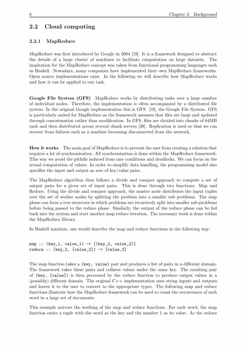
1 def map (name , document ) :2 for word in document do3 EmitIntermediate (w, 1)4
5 def reduce (word , par t ia lCount s ) :6 r e s = 07 for pc in par t ia lCount s :8 r e s = r e s + pc9 Emit ( r e s )
Listing 2.1: MapReduce Example
function is operating on all values of a single key, it just sums up the 1’s from each individualword and returns the total number of appearances. The partialCounts variable is an iteratorwhich walks over the output from the map function as written to the distributed file system.
Besides the map and reduce functions we further have an input reader which reads from thefile system and produces the input tuples for the map function. These tuples are split into aset of M splits and processed in parallel by the worker nodes. The partitioning for the reducenodes is similar. We specify a partitioning function like hash(key) mod R to do this. Thepartitioning function is used to split the data into R regions when buffered data from the maptasks is written to stable storage. The master is notified and then notifies the reduce tasks tostart working. Because the hash function can map multiple keys to one region, we need to sortthe data at the reduce node before we can process region R. Finally an output writer takesthe output of the reduce function and writes it to stable storage.
In some cases it is advisable to put a combiner function in between the map and reduce stages tolimit the amount of data passed on to the network layer. This can be seen in the word countingexample, where given the input language of the documents is English, there will be a lot of("the", 1) pairs emitted. The combiner function acts like the reduce step, the difference beingthat the algorithm writes its output to an intermediate file, whereas the output of the reducestep is written to the final output file.
As is tradition with Google, MapReduce clusters typically consist of large clusters of commodityPCs networked via ordinary switched Ethernet. Network failures are common, therefore, thealgorithm has to be very failure tolerant. By ensuring that individual operations are independent,it is easy to reschedule map operations in case of failure. However, we must be more carefulwhen output of a failed map has already been partially consumed by a reduce operation. In thiscase the reduce has to be aborted and rescheduled, too.
So far we have assumed that the map and reduce operations are independent. This restrictionallows us to make full use of the distributed system as these operations can all be executed inparallel without any significant locking overhead. The restriction is that the data has to beavailable to the processing units without any significant delay. In the original implementation,a reduce task for example needs all the data for a particular key to be presented at the sametime. To be able to process streams efficiently, we need to get rid of this restriction. As thisrestriction was implemented using a write to the distributed file system GFS, we need to streamdata from mappers to reducers instead. The details of this are discussed in §2.3.4.
Criticism / Evaluation Our choice in favour of MapReduce is motivated by the ease of useof its programming model and the tight integration with the cloud paradigm. The MapReducedesign provides natural support for scalability with its mappers and reducers. However, therehas been some criticism voiced over its implementation. Notably, David DeWitt and Michael
10 Chapter 2. Background
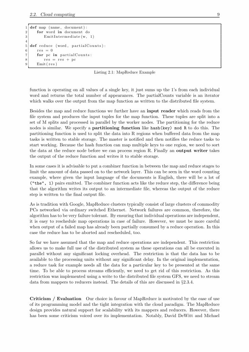
1 count : t ab l e sum of i n t ;2 t o t a l : t ab l e sum of f l o a t ;3 sum of square s : t ab l e sum of f l o a t ;4 x : f l o a t = input ;5 emit count <− 1 ;6 emit t o t a l <− x ;7 emit sum of square s <− x ∗ x ;
Listing 2.2: Sawzall Example
Stonebraker, two proponents of distributed databases have criticised MapReduce for its lack ofexpressiveness [22]. They argue that the programming model is outdated and not able to utiliseany of the performance improvements known from traditional databases such as indexing. Weargue that although DeWitt and Stonebraker are right on the limited expressiveness, they missthe point on the purpose of MapReduce. MapReduce is an excellent way to process a largeamount of data that comes in a relatively unstructured form. Once we have processed the data,we can store it in relational tuples and evaluate it further using a traditional database approach.The two approaches are therefore complimentary, a result that Stonebraker et al. acknowledgein a later paper [36]. They refer to the pre-processing stage as extract-transform-load tasksand call them a MapReduce speciality. In our project we will evaluate relational tuples as weexpect the difference between MapReduce and distributed database systems to be negligible insingle-query environments.
2.2.2 Sawzall
DeWitt and Stonebraker also criticised MapReduce for its lack of high level query language.Recently, there have been several efforts to remedy this. Sawzall is a domain specific procedurallanguage developed by Google to lie on top of the MapReduce framework. This language takesthe MapReduce approach further to make sure that its programmers write parallel code. It uses aset of aggregators “to capture many common data processing and data reduction problems” [34].As Sawzall is an interpreted language, we might think this would pose a significant constraint ina high performance environment. However, as the algorithms mainly spend time on I/O and theunderlying methods are implemented natively, this does not incur any significant penalty. Theincrease in performance when adding machines is almost linear. As we need more control overthe communication between the hosts to implement our stream processing paradigm, we cannotuse Sawzall to program the cloud infrastructure. However, this is an interesting approach andit might be considered to extend Sawzall to enable stream processing as the authors suggest.
The following simple Sawzall program (Listing 2.2) takes as input a set of records containingone floating point number each. It then produces three results. The total number of records,the sum of all the floating point values and the sum of the squares of the floating point numbers.
This looks very similar to the map phase as we have seen in the discussion of MapReducein §2.2.1. Here we define three aggregators: count, total and sum of squares. By definingthese aggregators as sum tables we tell Sawzall what the reduce part of MapReduce should bedoing. By pre-defining the aggregators, Sawzall relieves the programmer of the reduce taskbut also somewhat limits the expressiveness of map reduce. However, the upside is that theaggregators can now be implemented natively. Furthermore, the parallelism is hidden from theuser. Aggregators have to be commutative, associative and efficient for distributed programming.Extending the set of aggregators is therefore difficult.
2.2. Cloud computing 11
Evaluation Sawzall is a very interesting approach to take MapReduce more en par withtraditional database systems. By designing a domain specific language it is possible to furtherabstract and simplify parallel programming. At this stage, Sawzall is not yet able to expressstreaming queries. However, we will keep MapReduce DSL approaches in mind for furtherprojects.
2.2.3 Hadoop
Hadoop is the umbrella project for several Apache projects which have the aim to provide areliable platform for distributed computing. The Hadoop project can be split into two parts.The first is an implementation of MapReduce. Although the framework is written in Java, itaccepts MapReduce tasks written in other languages [1]. Similarly to Google’s Sawzall effort,the Hadoop project also includes Pig [28], a high level data-flow language to describe parallelprocesses. Pig’s compiler produces a chain of MapReduce operations. The language layer iscalled Pig-latin. The second part of the Hadoop implementation is the Hadoop Distributed FileSystem (HDFS), a file system, similar to GFS as employed in MapReduce [19]. Both HDFS andGFS are optimised for batch processing.
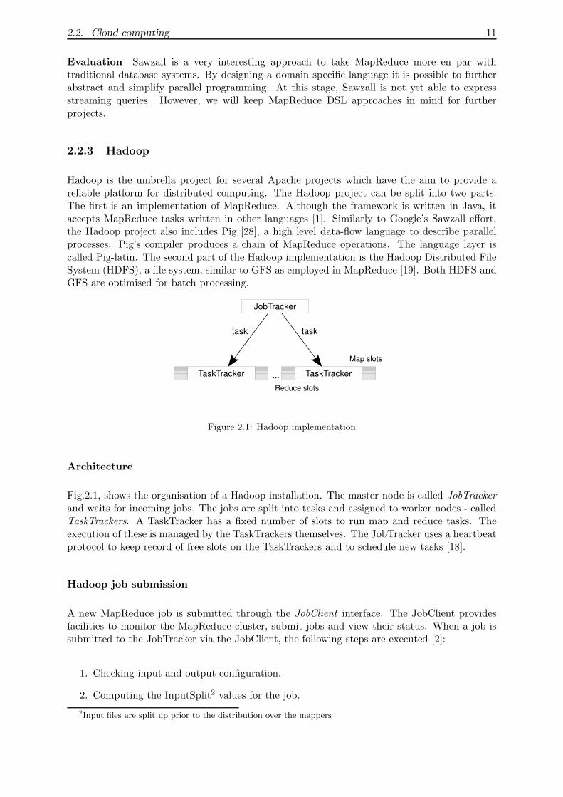
Figure 2.1: Hadoop implementation
Architecture
Fig.2.1, shows the organisation of a Hadoop installation. The master node is called JobTrackerand waits for incoming jobs. The jobs are split into tasks and assigned to worker nodes - calledTaskTrackers. A TaskTracker has a fixed number of slots to run map and reduce tasks. Theexecution of these is managed by the TaskTrackers themselves. The JobTracker uses a heartbeatprotocol to keep record of free slots on the TaskTrackers and to schedule new tasks [18].
Hadoop job submission
A new MapReduce job is submitted through the JobClient interface. The JobClient providesfacilities to monitor the MapReduce cluster, submit jobs and view their status. When a job issubmitted to the JobTracker via the JobClient, the following steps are executed [2]:
1. Checking input and output configuration.
2. Computing the InputSplit2 values for the job.
2Input files are split up prior to the distribution over the mappers
12 Chapter 2. Background
3. Copying the job’s jar and configuration to the MapReduce system directory on the filesystem.
4. Submitting the job to the JobTracker and monitoring its status.
Evaluation Hadoop is available on as cloud images and a standalone application and thereforeinteresting to our project. This and the amount of supporting tutorial material for Hadoopconvinced us to choose it for the MapReduce implementation. In its original design it does notallow for streaming MapReduce. This limitation is covered in §2.3.4.
2.2.4 Remote Procedure Calls
As distributed systems like Hadoop have to communicate intermediate results and to coordinatetheir behaviour, they need a reliable way to communicate. In Hadoop, a lot of inter-processcommunication is done using RMI, the Java version of a Remote Procedure Call (RPC). RPCis a technology to lookup functions outside the address space of the current process [30]. Thiscould mean a function on the same node, implemented by a class running in a different process,or code running on a different machine altogether. In either case, once the function has beenbound by the RPC framework on the local machine, a call behaves (almost) exactly like youwould expect it to on a local machine.
Implementation
A remote procedure call initialised and executed through message-passing [39]. The client nodefirst sends a request to the server process containing a unique identifier for the function to becalled. In order to find the server implementing the function, the calling process might eitherbroadcast a message on the local network or request a list of implementations from a well knownname server. In the latter case, it is necessary for the server process to register its implementationfirst. Once the client has completed the lookup phase for the particular function, it is bound toa local stub and can be used by the rest of the program. On the server side, a daemon ensuresthat all communication request are dealt with by either spawning a new thread or picking onefrom a pre-initialised thread pool.
Serialisation
RPC libraries can easily deal with most basic data types such as integers and strings. However,if we wish to call methods on complicated objects by reference, we need to make sure that theremote host is aware of these objects first. We need to serialise the object [39]. Serialisationof an object such as a linked list means traversing all the pointers and essentially flatteningthe datastructure such that it can be either saved to disk or transmitted over the network.Flatting complex datastructures is not always an easy task as we must follow all referenceswithout looping forever due to back edges in the graph. Furthermore, we cannot merely sendthe contents of the objects over the network as any pointer variables will not have the samemeaning on a remote host. The solution to this problem is called pointer swizzling. In ourexample of a linked list, we would for example introduce a new field to every node holding aunique identifier. We can then set the pointer to the next node to its identifier rather thanthe address in memory. This process can be easily reversed at the other side. However, thereis an cost associated with this operation. Thus, serialisation should not be used extensively
2.2. Cloud computing 13
when communicating in an environment where runtime is critical. When applicable, simplerdatastructures should be used.
Java RMI
Remote method invocation (RMI) is Java’s implementation of the RPC protocol. Instead ofpublishing information on a single method with a nameserver, the callee registers its remoteobject with the RMI-Registry under a unique identifier [37]. The client program can now querythe RMI-Registry with this identifier to get a reference to the remote object. This reference hasto be an implementation of its remote interface. The remote interface defines the methods thatare guaranteed to be implemented by the remote object. The client can now call the methodson the remote object as published by the remote interface. It is possible for the method headersof the remote object to contain references to interfaces. Any class implementing these interfacesmay then be used on the remote host including class definitions from the caller. This meansthat Java gives the user the opportunity to dynamically load new code as part of a RMI call.In order to make sure that this is not exploited for malicious use, a security manager is alwaysinstalled as part of the RMI implementation. Any special requests have first to be granted bythe designer of the server application.
2.2.5 Amazon EC2
Despite having chosen to implement our stream processor on cluster nodes in the college, ourultimate aim is to run stream processing on an IaaS platform such as Amazon EC2. The decisionto develop and test locally has been purely a development one. However, as all our machinesare single-purpose and only used for this project, our setup is not too dissimilar to a “cloud”.The participating nodes are running the same specifications. In fact, the EC2 technology isavailable as part of the Ubuntu Eucalyptus packages and can be integrated into an Ubuntuserver installation. It could thus be easily installed on our test cluster.
Amazon’s EC2 offering, introduced in 2006 [11], was one of the first commercial cloud infras-tructures. EC stands for Elastic Cloud. Customers are allowed to create an Amazon MachineImage. This image is used to start a virtual machine on the Amazon cluster. The infrastructureallows customers to start and terminate new virtual machines as required by the application,hence the term elastic. Additional nodes can be accessed within minutes. This ease of usemakes it very interesting for our purposes of load balancing. Amazon charges by the hour orthe data transfer rate. Further charges are possible. The various virtual machines instances asof December 2009 are shown below. These instances are based on the notion of EC2 ComputeUnits. The units mirror equivalent capacity of physical hardware. It is possible to specify thegeographical location of the servers in order to optimize network latency and fault tolerance.
1. Small Instance (Default) 1.7 GB of memory, 1 EC2 Compute Unit (1 virtual core with1 EC2 Compute Unit), 160 GB of local instance storage, 32-bit platform
2. Large Instance 7.5 GB of memory, 4 EC2 Compute Units (2 virtual cores with 2 EC2Compute Units each), 850 GB of local instance storage, 64-bit platform
3. Extra Large Instance 15 GB of memory, 8 EC2 Compute Units (4 virtual cores with 2EC2 Compute Units each), 1690 GB of local instance storage, 64-bit platform
14 Chapter 2. Background
The Amazon CloudWatch service gives information about the current load on the system. Thisinformation can be accessed via a web service or web APIs. Unfortunately, this service incursa charge for the number of monitoring instances used. However, the CloudWatch service isnecessary for using the auto scaling feature of EC2. Auto-scaling enables us to specify triggerswhich cause Amazon to add or remove instances automatically.
Persistent storage on EC2 systems is provided using the Amazon Simple Storage (S3) service.The EC2 implementation itself only stores temporary data. If an instance is rebooted, this datais lost. As this can happen explicit via an API call or a failure in the system, we cannot ensurefault-tolerance without a form of persistent storage. Google’s MapReduce algorithm requires adistributed file system to store the intermediate results. The S3 service makes data availabledirectly to the EC2 instances and over the network via http. This makes it suitable for ordinaryMapReduce. For low latency access, we must use S3 and EC2 services in the same area. Thereis no extra cost for S3 to EC2 bandwidth. Despite its advantages and close link to the originalMapReduce idea, the distributed file system is more of an obstacle towards efficient streamprocessing as both input and output should be written to sockets rather than to stable storage.
2.3 Stream processing
In this section we are covering several research prototypes of stream processing, ranging fromsingle node implementations to distributed versions. The goal of the project is to focus on theload-balancing between the front-end node and the processing power of the cloud. In this light,we will evaluate the state of the art and rationalise our decision to use a MapReduce frameworkto do stream processing in a cloud environment.
2.3.1 Mortar
Logothethis and Yocum have developed Mortar - “A distributed stream processing platform forbuilding very large queries” [29]. The Mortar platform focuses on applications with thousandsof distributed sources. It takes into account unreliable sources and adverse network connections.Mortar is designed to manage streaming queries across large federated systems3. The Mortarinfrastructure takes over the task of creating and removing operators as well as organising thedata flow between them. For this reason, one of the main contributions of the above paper isto provide robust overlay networks to run queries. Mortar also addresses the problem of timesynchronisation between the different nodes. Stream processing cannot work without reliabletime information as the timestamps used for windows become useless. Mortar differentiatesitself from the other approaches shown here, as not only are the data-supplying nodes involvedin the processing, but the designers want them to be the only ones to do the work. Logothetisand Yocum speak of scoped queries in this context. We now discuss the overlay networks androuting algorithm employed by Mortar.
Overlay network The overlay networks in Mortar are static. The authors justify this bythe claim that in federated systems, machines are rarely added or removed. They can onlybecome unavailable for a short time. It is assumed that there is personnel in charge of thesites which quickly rectifies any problems. However, in order to deal with failures, multiplestatic trees are created and operators are connected across them. The static aggregation treesin the Mortar framework are build such that the majority of nodes is close to the root node.
3Federated systems typically include heterogeneous hardware and different authorities
2.3. Stream processing 15
This is necessary to ensure the latency bounds required by streaming applications. Once theprimary tree is built, the sibling trees are derived through successive random rotations of internalsubtrees. The authors have confirmed by empirical observation, that this is unlikely to changethe clustering.
Dynamic tuple striping The routing scheme proposed by Logothetis and Yocum is calleddynamic tuple striping. Dynamic striping is a multi-path routing scheme. Routing is done upthe trees towards the root. Since scoped queries are used, each node needs to know about alllive parents for locally installed queries. These are found using a heartbeat protocol. Childrenare updated in the same way. Tuples are routed through a parent only if this moves them closerto the root. The algorithm first tries to use the parent on the tree on which the tuple arrived.If this fails, it tries a parent on a different tree which must not be further away from the root asthe current tree. This avoids cycles. However, if no further progress could be made, a tuple isallowed to move down to a child and try a different path. As this now introduces the possibilityto incur cycles, a time to live field is introduced (TTL) to restrict the number of tries.
Evaluation Mortar has somewhat limited applicability to our cloud approach. As our chosenplatform is homogeneous and under a single administration we have eliminated most of theproblems stemming from federated systems. Indeed, the implementation of our chosen streamprocessor should be modifiable to run on virtual machines which might be added or removedduring the computation. This form of scalability is not what the authors of Mortar envisaged.Mortar is a very reliable platform for applications such as sensor networks with a large numberof data providing nodes. In these cases an overlay network is justified. In our case, however, itviolates the low latency requirements. Applying Mortar to stream processing in a cloud settingwould require too many modifications.
2.3.2 STREAM
STREAM is a data stream management system (DSMS) developed by the University of Stan-ford [9]. Ordinary database management systems (DBMS) deal with one-time queries. Networkmonitoring, financial analysis and sensor networks, however, emit a continuous stream of data.Thus in addition to ordinary relations, we have bags of tuple, timestamp pairs, called streams.Streams can only be handled by continuous queries. The STREAM project aims to fill thisgap. The prototype DSMS [9], supports a “large class of declarative continuous queries overcontinuous streams”. It evaluates the queries by translating the declarative queries into a phys-ical query plan. This plan is then processed by the DSMS. A query plan consists of operators,queues and synopses.
Operators Arasu et al. have developed the Continuous Query Language (CQL) [9]. CQLlooks very much like an extension to SQL. There are three types of operators: relation-to-relation, relation-to-stream and stream-to-relation. The relation-to-relation operators are thewell-known SQL operators. The stream-to-relation operators are more interesting. They offerthe ability to turn the continuous stream into a relation which can be modified by ordinaryrelational algebra. The stream-to-relation operators are following the sliding window concept.A tuple-based sliding window is expressed using [ROWS N] after the steam identifier. This returnsa relation with the last N tuples/rows in the stream. The [Range N] parameter gives a time-based sliding window. The relation returned includes all tuples with more than N timesteps in
16 Chapter 2. Background
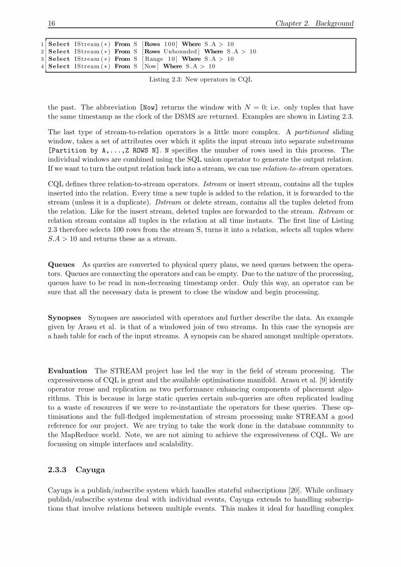
1 Select IStream (∗ ) From S [Rows 100 ] Where S .A > 102 Select IStream (∗ ) From S [Rows Unbounded ] Where S .A > 103 Select IStream (∗ ) From S [ Range 10 ] Where S .A > 104 Select IStream (∗ ) From S [Now] Where S .A > 10
Listing 2.3: New operators in CQL
the past. The abbreviation [Now] returns the window with N = 0; i.e. only tuples that havethe same timestamp as the clock of the DSMS are returned. Examples are shown in Listing 2.3.
The last type of stream-to-relation operators is a little more complex. A partitioned slidingwindow, takes a set of attributes over which it splits the input stream into separate substreams[Partition by A,...,Z ROWS N]. N specifies the number of rows used in this process. Theindividual windows are combined using the SQL union operator to generate the output relation.If we want to turn the output relation back into a stream, we can use relation-to-stream operators.
CQL defines three relation-to-stream operators. Istream or insert stream, contains all the tuplesinserted into the relation. Every time a new tuple is added to the relation, it is forwarded to thestream (unless it is a duplicate). Dstream or delete stream, contains all the tuples deleted fromthe relation. Like for the insert stream, deleted tuples are forwarded to the stream. Rstream orrelation stream contains all tuples in the relation at all time instants. The first line of Listing2.3 therefore selects 100 rows from the stream S, turns it into a relation, selects all tuples whereS.A > 10 and returns these as a stream.
Queues As queries are converted to physical query plans, we need queues between the opera-tors. Queues are connecting the operators and can be empty. Due to the nature of the processing,queues have to be read in non-decreasing timestamp order. Only this way, an operator can besure that all the necessary data is present to close the window and begin processing.
Synopses Synopses are associated with operators and further describe the data. An examplegiven by Arasu et al. is that of a windowed join of two streams. In this case the synopsis area hash table for each of the input streams. A synopsis can be shared amongst multiple operators.
Evaluation The STREAM project has led the way in the field of stream processing. Theexpressiveness of CQL is great and the available optimisations manifold. Arasu et al. [9] identifyoperator reuse and replication as two performance enhancing components of placement algo-rithms. This is because in large static queries certain sub-queries are often replicated leadingto a waste of resources if we were to re-instantiate the operators for these queries. These op-timisations and the full-fledged implementation of stream processing make STREAM a goodreference for our project. We are trying to take the work done in the database community tothe MapReduce world. Note, we are not aiming to achieve the expressiveness of CQL. We arefocussing on simple interfaces and scalability.
2.3.3 Cayuga
Cayuga is a publish/subscribe system which handles stateful subscriptions [20]. While ordinarypublish/subscribe systems deal with individual events, Cayuga extends to handling subscrip-tions that involve relations between multiple events. This makes it ideal for handling complex
2.3. Stream processing 17
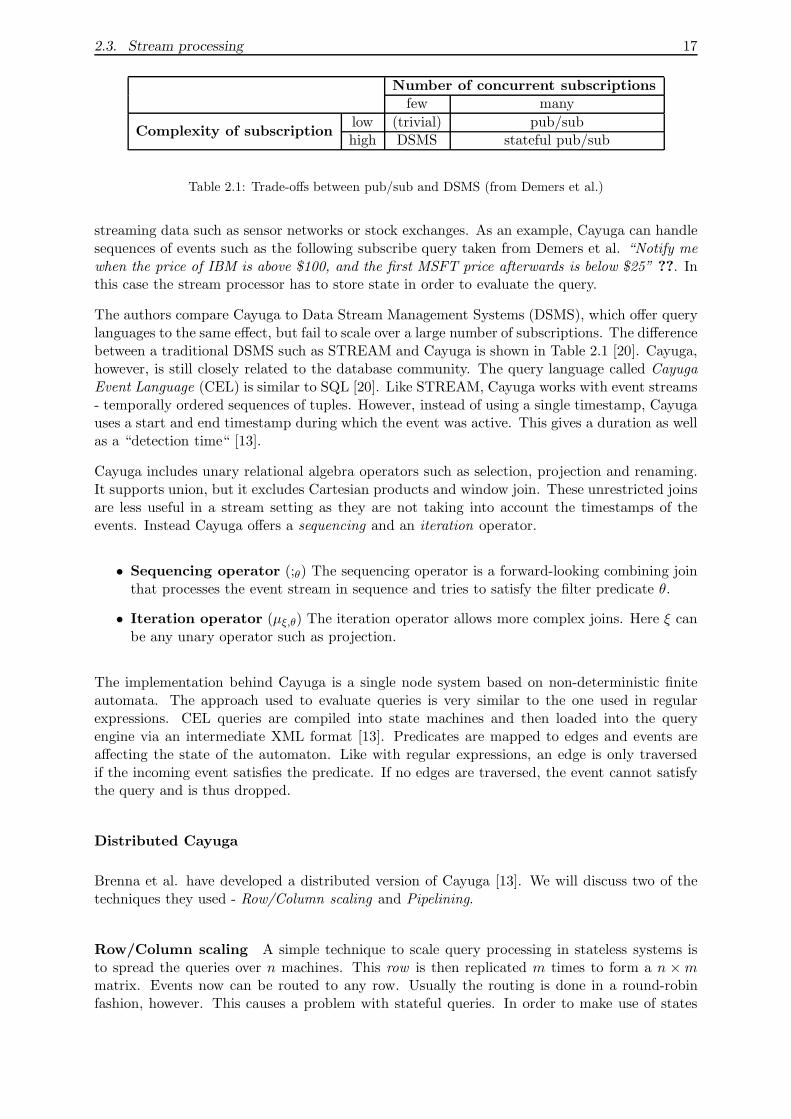
Number of concurrent subscriptionsfew many
Complexity of subscriptionlow (trivial) pub/subhigh DSMS stateful pub/sub
Table 2.1: Trade-offs between pub/sub and DSMS (from Demers et al.)
streaming data such as sensor networks or stock exchanges. As an example, Cayuga can handlesequences of events such as the following subscribe query taken from Demers et al. “Notify mewhen the price of IBM is above $100, and the first MSFT price afterwards is below $25” ??. Inthis case the stream processor has to store state in order to evaluate the query.
The authors compare Cayuga to Data Stream Management Systems (DSMS), which offer querylanguages to the same effect, but fail to scale over a large number of subscriptions. The differencebetween a traditional DSMS such as STREAM and Cayuga is shown in Table 2.1 [20]. Cayuga,however, is still closely related to the database community. The query language called CayugaEvent Language (CEL) is similar to SQL [20]. Like STREAM, Cayuga works with event streams- temporally ordered sequences of tuples. However, instead of using a single timestamp, Cayugauses a start and end timestamp during which the event was active. This gives a duration as wellas a “detection time“ [13].
Cayuga includes unary relational algebra operators such as selection, projection and renaming.It supports union, but it excludes Cartesian products and window join. These unrestricted joinsare less useful in a stream setting as they are not taking into account the timestamps of theevents. Instead Cayuga offers a sequencing and an iteration operator.
• Sequencing operator (;θ) The sequencing operator is a forward-looking combining jointhat processes the event stream in sequence and tries to satisfy the filter predicate θ.
• Iteration operator (µξ,θ) The iteration operator allows more complex joins. Here ξ canbe any unary operator such as projection.
The implementation behind Cayuga is a single node system based on non-deterministic finiteautomata. The approach used to evaluate queries is very similar to the one used in regularexpressions. CEL queries are compiled into state machines and then loaded into the queryengine via an intermediate XML format [13]. Predicates are mapped to edges and events areaffecting the state of the automaton. Like with regular expressions, an edge is only traversedif the incoming event satisfies the predicate. If no edges are traversed, the event cannot satisfythe query and is thus dropped.
Distributed Cayuga
Brenna et al. have developed a distributed version of Cayuga [13]. We will discuss two of thetechniques they used - Row/Column scaling and Pipelining.
Row/Column scaling A simple technique to scale query processing in stateless systems isto spread the queries over n machines. This row is then replicated m times to form a n × mmatrix. Events now can be routed to any row. Usually the routing is done in a round-robinfashion, however. This causes a problem with stateful queries. In order to make use of states
18 Chapter 2. Background
we must route events to the same row. This is infeasible. Brenna et al. [13] propose two waysof partitioning the workload.
The first technique is to partition the input event stream into several substreams of relatedevents. These substreams are then assigned to rows and processed individually. The partitioningitself can be expressed as a Cayuga query and done by a separate machine.
The second technique is to partition the query workload. Thus instead of sending substreamsto the rows, each row receives a full copy of the input stream.
Pipelining Cayuga provides the possibility for queries to be split into sub-queries if the formercan not be run on a single machine. The output of one subquery to another is controlled via afeature called re-subscription [13].
Evaluation Cayuga and the effort to run it over large distributed networks are two interestingapproaches. In the single node implementation Cayuga with its very expressive CEL languagemakes a lot of sense. However, in the distributed case, the situation is more complicated. Forour project we are planning to start with a single query which means that the ideas concerningrow/column scaling are currently not applicable.
2.3.4 MapReduce Online
MapReduce Online enables ”MapReduce programs to be written for applications such as eventmonitoring and stream processing“; it has been proposed in a technical report by Condie et al.in 2009 [18]. In contrast to the original Google implementation of MapReduce [19], Condie et al.propose a pipelined version in which the intermediate data is not written to disk. The prototypefor this concept is a modification of the Hadoop framework and called Hadoop Online Prototype(HOP).
The first change the authors introduced into stock Hadoop is pipelining. Instead of writing datato disk, it is now delivered straight from the producers (map tasks) to consumers (reduce tasks)via TCP sockets. If a reduce task has not been scheduled yet, the data can be written to disk asin plain Hadoop. The number of connections is also bounded to prevent creating too many TCPconnections. Combiners are facilitated by waiting for the map-side buffers to fill before they aresent to the reducers. This enables us to pre-process the data before it is sent to the reducers.The processed data is written to a spill file which is monitored by a separate thread. Thisthread transmits the data to the reducers. The spill files enable simple load balancing betweenthe mappers and reducers as their size and number reflects the load difference in the system. Ifspill files grow, we can adaptively invoke a combiner function on the side of the mapper to eventhe load.
The Hadoop Online Prototype further allows for inter-job pipelining. It must be noted that itis impossible to overlap the previous reduce with the current map function as the former has tocomplete before the latter can start. However, pipelining reduces the necessity to store interme-diate result in stable storage which could be costly. Condie et al. have extended Hadoop to beable to insert jobs ”in order“. This helps to preserve dataflow dependencies. The introductionof pipelining into Hadoop makes the system ready for running streaming applications.
2.4. Load balancing 19
Evaluation The Hadoop Online Prototype is a very interesting approach for stream process-ing. The changes over ordinary MapReduce implementations are subtle but powerful. However,like all other technologies visited in this section, HOP does not automatically scale during run-time. The number of map and reduce tasks is fixed. This impairs the ability of the MapReduceimplementation to cope with varying load. We have chosen to use Hadoop as a starting pointto design a stream processor utilising the MapReduce paradigm.
2.4 Load balancing
Load balancing is an integral part of our system’s design. A single stream processing nodeshould automatically move computation to the cloud when its own resources are not sufficientanymore. In this project we aim to do this in a way which avoids an increase in latency and givesa guarantee on QoS properties of the system. To find possible strategies to achieve this, we havestudied several load balancing strategies for webservers. First there are client side policies inwhich the client decides which server to use. Client-side policies include NRT (network round-trip-time) and latency estimated from historical data [14]. Selection algorithms are also basedon hop count or geographical distance. We are also interested in server side policies which use aload index to determine how to route requests. Both are applicable as we run the local streamprocessor and evaluate its load on the same machine. However, none of the research mentionedin this section is 100 percent applicable to our situation. We are not aware of a load-balancingsolution that evaluates computational load at a single front-end node and moves the overheadinto a scalable cluster.
2.4.1 Load-balancing in distributed web-servers
Cardellini et al. discussed the state of the art in locally distributed web-server systems [15].While our load-balancing or load-sharing algorithm is located at layer 7 (i.e. application layer ofthe OSI model) this paper gives insights into routing at all layers. We are especially interestedin the discussion of a proxy for routing the requests (TCP gateway) and the discussion aboutdispatching algorithms. In our use-case we are looking for a load sharing algorithm that smoothsout transient peak overload. This algorithm must be dynamic as we require it to have informationabout the state of the system. Finally, we must decide between centralised and distributedalgorithms. As we will do the load balancing on the single machine serving as a controller tothe cloud computations and the initial worker node, we opt for a centralised algorithm here.
As mentioned in the article, fundamental questions are which server load index to use, when tocompute it and how this index is shared with the orchestrating server. Ferrari and Zhou foundthat load indices based on queue length perform better than load indices based on resourceutilisation [23]. They define the load index as a positive integer variable. It is 0 if the resource isidle and increases with more load. We must further acknowledge that there is no general notionof load. For example the CPU might be idle in a heavily I/O bound process, while in other casesprocesses are competing for CPU time. To summarise, the following load indices are mentionedin Ferrari and Zhou [23].
• CPU queue length
• CPU utilisation
• Normalised response time4
4response time of job on loaded machine / response time on idle machine
20 Chapter 2. Background
Evaluation Our load balancing exercise will mainly concentrate on the local node as forthe cloud this should be done by the MapReduce framework. This means that we can easilycalculate the normalised response time. If this time exceeds a certain threshold we can startmoving computational load to the cloud. Queue length is also a good indicator of load. In theevaluation chapter of this report we shall look at both response time and queue length.
2.4.2 Locally aware request distribution
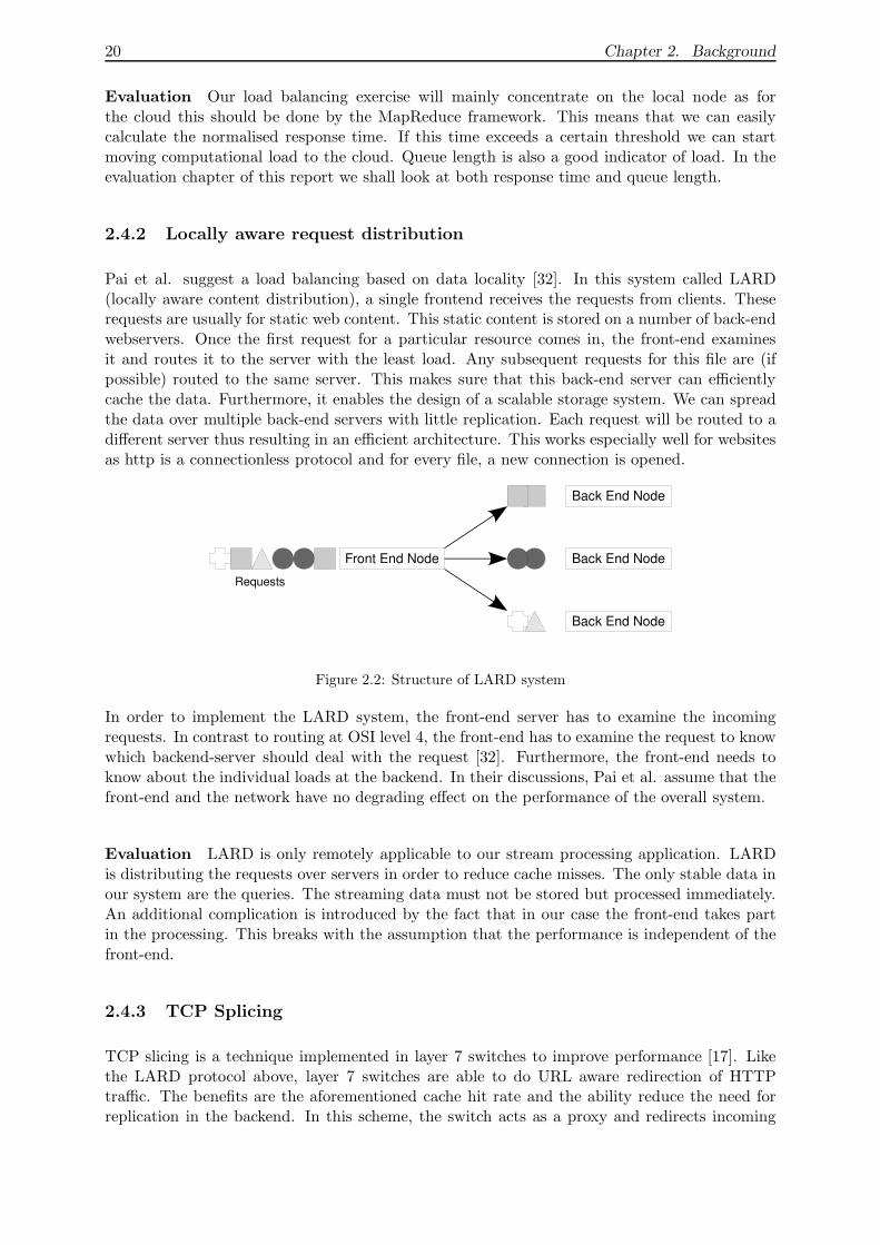
Pai et al. suggest a load balancing based on data locality [32]. In this system called LARD(locally aware content distribution), a single frontend receives the requests from clients. Theserequests are usually for static web content. This static content is stored on a number of back-endwebservers. Once the first request for a particular resource comes in, the front-end examinesit and routes it to the server with the least load. Any subsequent requests for this file are (ifpossible) routed to the same server. This makes sure that this back-end server can efficientlycache the data. Furthermore, it enables the design of a scalable storage system. We can spreadthe data over multiple back-end servers with little replication. Each request will be routed to adifferent server thus resulting in an efficient architecture. This works especially well for websitesas http is a connectionless protocol and for every file, a new connection is opened.
Figure 2.2: Structure of LARD system
In order to implement the LARD system, the front-end server has to examine the incomingrequests. In contrast to routing at OSI level 4, the front-end has to examine the request to knowwhich backend-server should deal with the request [32]. Furthermore, the front-end needs toknow about the individual loads at the backend. In their discussions, Pai et al. assume that thefront-end and the network have no degrading effect on the performance of the overall system.
Evaluation LARD is only remotely applicable to our stream processing application. LARDis distributing the requests over servers in order to reduce cache misses. The only stable data inour system are the queries. The streaming data must not be stored but processed immediately.An additional complication is introduced by the fact that in our case the front-end takes partin the processing. This breaks with the assumption that the performance is independent of thefront-end.
2.4.3 TCP Splicing
TCP slicing is a technique implemented in layer 7 switches to improve performance [17]. Likethe LARD protocol above, layer 7 switches are able to do URL aware redirection of HTTPtraffic. The benefits are the aforementioned cache hit rate and the ability reduce the need forreplication in the backend. In this scheme, the switch acts as a proxy and redirects incoming
2.5. Summary 21
HTTP requests based on the URI in the GET request. Incoming requests are examined andand the switch queries the right backend server for the response.
While layer 4 switching is based on port and IP, layer 7 switches work at the application layer.As application data is only transferred once the connection has been established we cannot doURI aware routing without first establishing a connection between the client and the switch.This means that we need to establish two connections. The first connection is between theclient and the switch. The second connection is between the switch and the backend server.The most common form of handling this problem is called TCP gateway. The TCP gatewaysolution simply forwards the packets from the backend over the switch at the application layer.However, this is unnecessary. Once we have established the connection between the client andthe switch and located the right backend server, any subsequent reply from the backend canbe forwarded over layer 4. This technique is called TCP splicing. Packets from the server tothe switch are translated to look as if they had passed through the application layer in theTCP gateway protocol. As we do not have to examine the content but only to rewrite sequencenumber addresses, this is relatively simple and can be done with little to no overhead. TCPslicing is very effective for large files as the number of outgoing packets is much greater than theincoming requests. But even for data as small as 1Kb, significant performance benefits can beobtained [17].
Evaluation TCP slicing only concerns how the data is being handled by the switch. Theactual load balancing is not affected. This technique is very interesting for us as we will need toredirect the output from the cloud to the clients. However, the response is likely to be shorterthan the incoming data (as discussed above). Furthermore, we cannot afford to create too muchoverhead in the local server as we would like to use it for processing as well. An interesting casearises when the amount of work done in the cloud eclipses the work done locally by a few times.In this case, the local machine may become merely a coordinator and the TCP slicing solutionviable.
2.5 Summary
In this chapter we have covered the design principles of the MapReduce framework. We havediscussed the original paper by Google [19] and a streaming variant called HOP based on theHadoop framework [18]. We will be using the MapReduce paradigm to design a scalable streamprocessor. The discussion on remote procedure calls (RPC) serves to give the necessary back-ground for the custom MapReduce prototype introduced in Chapter 4. The short introductionto Amazon’s EC2 should remind us of the ultimate goal which is to move the auxiliary streamprocessor to an IaaS provider. We have reviewed the current state of the art in stream processingand hinted why none of the existing systems are designed to be used on a cloud infrastructure.This chapter was concluded with an overview of some existing load balancing techniques andtheir limitations when applied to our specific situation. We are not aware of a load-balancing so-lution which supports a single-node stream processor through an auxiliary, scalable, cloud-basedstream processor.

22 Chapter 2. Background
Chapter 3
Stream Processing With Hadoop
In this chapter we will discuss our efforts to extend the MapReduce paradigm to continuousqueries. We will show the design and implementation process leading to a MapReduce streamprocessor which can be run on a cloud infrastructure. We will start by showing how we canextend Hadoop to accept a TCP stream as a data source. We will then discuss how the conceptof jobs can be extended to continuous queries. This chapter will be concluded with a discussionon the architectural limitations of Hadoop as a stream processor. The evaluation of our resultswill follow in Chapter 6.
3.1 From batch to stream processing
We have chosen Hadoop as the basis for our streaming MapReduce as it has already been adoptedin a range of industry projects [10] [25] [35]. The main advantage of this is that the acceptanceof a streaming solution is likely to be greater with this already proved software. Hadoop isopen-source software and therefore amenable for extensions and modifications.
The key to our evaluation of the MapReduce framework will be the guarantees given on latencyand the capability to scale efficiently as the load is increased.
Hadoop is designed for batch-processing. A typical Hadoop job takes hours and is run ondozens of machines [19]. A query in a stream processing system must typically be executed inseconds or milliseconds. Therefore, some modifications are necessary to adopt Hadoop for streamprocessing. As discussed in the background section (see §2.2.3 and §2.3.4), we shall be using amodified version of Hadoop, the Hadoop Online Prototype [18] (HOP), for our experiments.
There are two main tasks, we need to achieve before we can use Hadoop to process continuousdata streams:
1. Network I/O Hadoop needs to be able to forgo the distributed file system and read itsdata straight from a network socket. Likewise, the output of the MapReduce operationhas to be written to a socket for delivery to the client.
2. Persistent queries Hadoop is designed to accept one job per input directory. We cansubmit many jobs in succession, but there it is currently impossible to install a persistentquery.
23
24 Chapter 3. Stream Processing With Hadoop
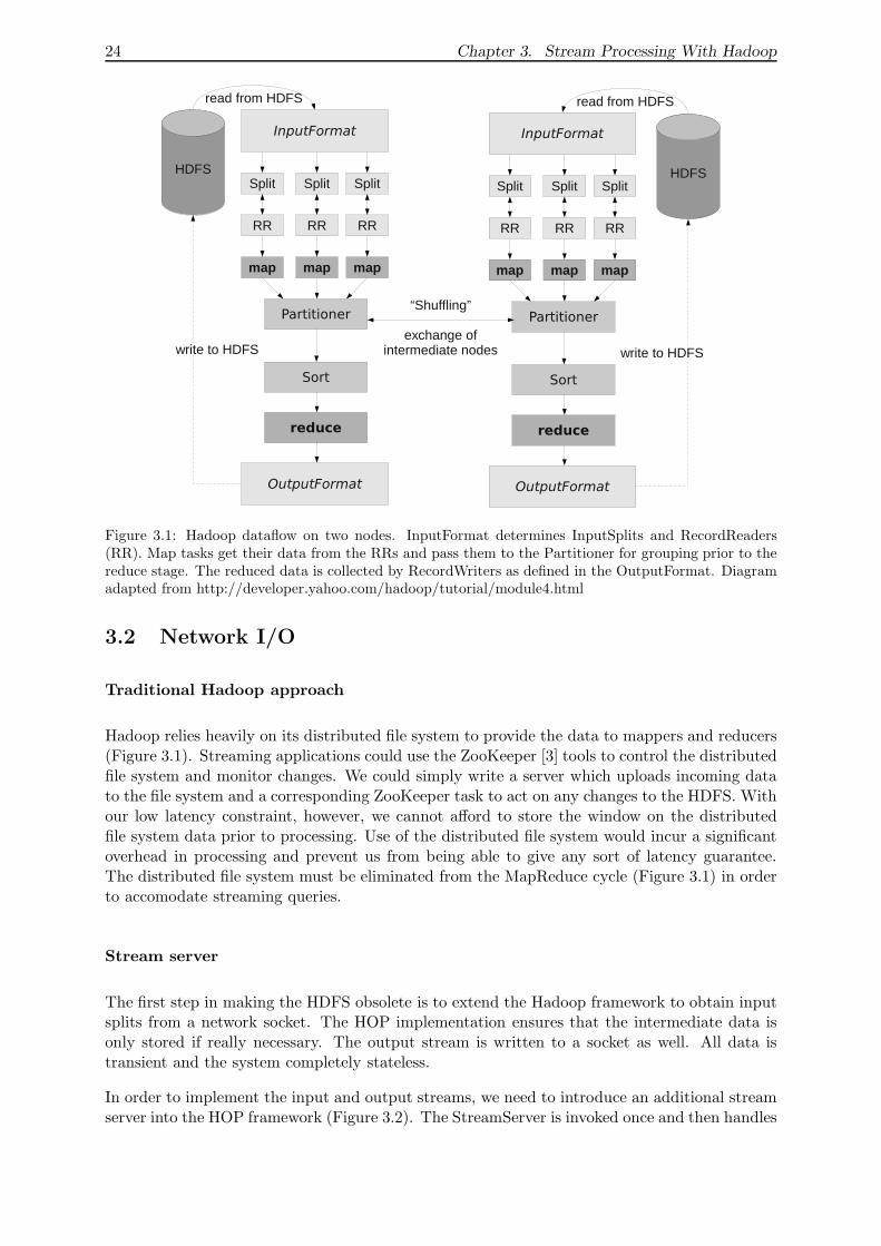
Figure 3.1: Hadoop dataflow on two nodes. InputFormat determines InputSplits and RecordReaders(RR). Map tasks get their data from the RRs and pass them to the Partitioner for grouping prior to thereduce stage. The reduced data is collected by RecordWriters as defined in the OutputFormat. Diagramadapted from http://developer.yahoo.com/hadoop/tutorial/module4.html
3.2 Network I/O
Traditional Hadoop approach
Hadoop relies heavily on its distributed file system to provide the data to mappers and reducers(Figure 3.1). Streaming applications could use the ZooKeeper [3] tools to control the distributedfile system and monitor changes. We could simply write a server which uploads incoming datato the file system and a corresponding ZooKeeper task to act on any changes to the HDFS. Withour low latency constraint, however, we cannot afford to store the window on the distributedfile system data prior to processing. Use of the distributed file system would incur a significantoverhead in processing and prevent us from being able to give any sort of latency guarantee.The distributed file system must be eliminated from the MapReduce cycle (Figure 3.1) in orderto accomodate streaming queries.
Stream server
The first step in making the HDFS obsolete is to extend the Hadoop framework to obtain inputsplits from a network socket. The HOP implementation ensures that the intermediate data isonly stored if really necessary. The output stream is written to a socket as well. All data istransient and the system completely stateless.
In order to implement the input and output streams, we need to introduce an additional streamserver into the HOP framework (Figure 3.2). The StreamServer is invoked once and then handles
3.2. Network I/O 25
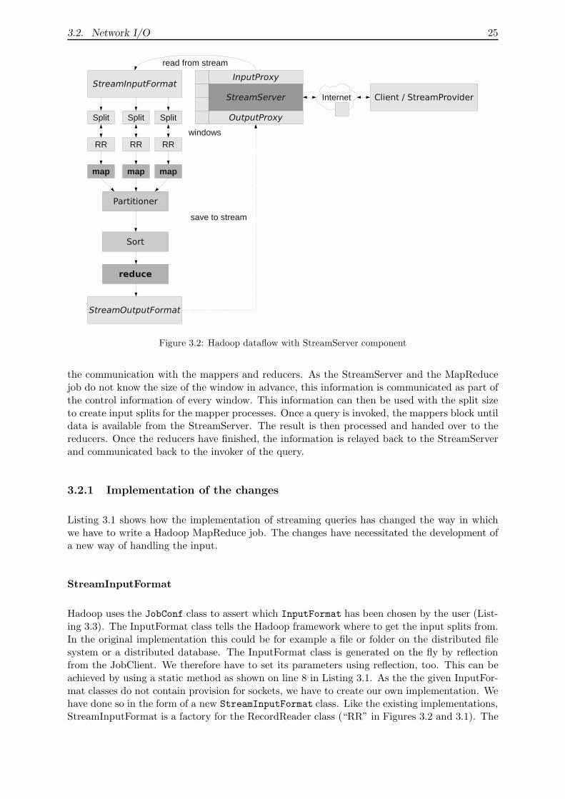
Figure 3.2: Hadoop dataflow with StreamServer component
the communication with the mappers and reducers. As the StreamServer and the MapReducejob do not know the size of the window in advance, this information is communicated as part ofthe control information of every window. This information can then be used with the split sizeto create input splits for the mapper processes. Once a query is invoked, the mappers block untildata is available from the StreamServer. The result is then processed and handed over to thereducers. Once the reducers have finished, the information is relayed back to the StreamServerand communicated back to the invoker of the query.
3.2.1 Implementation of the changes
Listing 3.1 shows how the implementation of streaming queries has changed the way in whichwe have to write a Hadoop MapReduce job. The changes have necessitated the development ofa new way of handling the input.
StreamInputFormat
Hadoop uses the JobConf class to assert which InputFormat has been chosen by the user (List-ing 3.3). The InputFormat class tells the Hadoop framework where to get the input splits from.In the original implementation this could be for example a file or folder on the distributed filesystem or a distributed database. The InputFormat class is generated on the fly by reflectionfrom the JobClient. We therefore have to set its parameters using reflection, too. This can beachieved by using a static method as shown on line 8 in Listing 3.1. As the the given InputFor-mat classes do not contain provision for sockets, we have to create our own implementation. Wehave done so in the form of a new StreamInputFormat class. Like the existing implementations,StreamInputFormat is a factory for the RecordReader class (“RR” in Figures 3.2 and 3.1). The
26 Chapter 3. Stream Processing With Hadoop
1 StreamServer . s t a r t S e rv e r (50002) ;2 // Create a new job /query con f i gu r a t i on3 JobConf conf = new JobConf ( StreamDriver . class ) ;4 // Set the input to a stream5 conf . setInputFormat ( StreamInputFormat . class ) ;6 conf . setOutputFormat ( StreamOutputFormat . class ) ;7 // Connect the stream to the StreamServer8 StreamInputFormat . setInputStream ( conf , ” l o c a l h o s t ” , 50002 , 10000) ;9 StreamOutputFormat . setOutputStream ( conf , ” l o c a l h o s t ” , 50001) ;
10 // Set the query11 conf . setMapperClass ( StreamMapper . class ) ;12 conf . setReducerClass ( StreamReducer . class ) ;13 try {14 JobCl ient . runJob ( conf ) ;15 } catch ( Exception e ) {16 e . pr intStackTrace ( ) ;17 }
Listing 3.1: Driver method: The StreamServer component listens on a user-defined port. Instead of theusual input format, based on the distributed file system, we introduce a new StreamInputFormat classthat handles the provision of key/value pairs to the mappers. As the mappers are dynamically requestingthe information, we cannot connect them directly to the input stream. Instead they are connected tothe StreamServer proxy, which handles the connection to the client. This is similar to the way in whichHadoop handles input from a database system.
RecordReader gives the mappers access to the input data. In the original implementations, atypical return value of the RecordReader’s next() method could be a line of output. For eachMapTask, we have a separate RecordReader.
StreamRecordReader
Our StreamInputFormat class returns a StreamRecordReader. The StreamRecordReader usesa socket to connect to the StreamServer’s output proxy. This is done as soon as the Stream-RecordReader is initialised. A call to the next() function will then return a tuple from the inputbuffer. If the input buffer is empty, the call blocks. The StreamRecordReader stops providingdata once the current window has been exhausted. The MapTask is notified. Hadoop uses aDataInput object to wrap around the InputStream. The DataInput class is used to tell theRecordReader about the size of the next input. This is not necessary in our case as we controlthe size of the output from the StreamServer’s output proxy ourselves. Once the MapTaskhas received the data, the operation is the same as in the stock HOP/Hadoop implementation.The output from the MapTasks is collected by an OutputCollector and distributed for the re-duce phase. Once the reducers have finished their task, the data needs to be send back to theStreamServer.
StreamOutputFormat
The StreamOutputFormat class is very similar in style to the StreamInputFormat. Instead ofa RecordReader, it contains a factory method to create a RecordWriter. Again, no provisionis given in the original implementation of Hadoop for writing output to a socket. We haveimplemented a new class StreamOutputFormat which handles this. The StreamOutputFormatprovides a StreamRecordWriter which like the reader connects to a proxy at the StreamServerto deliver its data. The data is then routed via the StreamServer back to the client. The param-
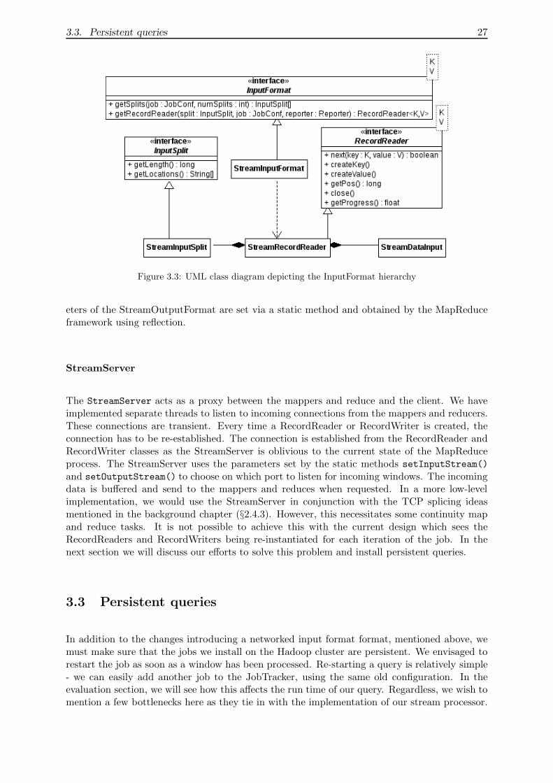
3.3. Persistent queries 27
Figure 3.3: UML class diagram depicting the InputFormat hierarchy
eters of the StreamOutputFormat are set via a static method and obtained by the MapReduceframework using reflection.
StreamServer
The StreamServer acts as a proxy between the mappers and reduce and the client. We haveimplemented separate threads to listen to incoming connections from the mappers and reducers.These connections are transient. Every time a RecordReader or RecordWriter is created, theconnection has to be re-established. The connection is established from the RecordReader andRecordWriter classes as the StreamServer is oblivious to the current state of the MapReduceprocess. The StreamServer uses the parameters set by the static methods setInputStream()
and setOutputStream() to choose on which port to listen for incoming windows. The incomingdata is buffered and send to the mappers and reduces when requested. In a more low-levelimplementation, we would use the StreamServer in conjunction with the TCP splicing ideasmentioned in the background chapter (§2.4.3). However, this necessitates some continuity mapand reduce tasks. It is not possible to achieve this with the current design which sees theRecordReaders and RecordWriters being re-instantiated for each iteration of the job. In thenext section we will discuss our efforts to solve this problem and install persistent queries.
3.3 Persistent queries
In addition to the changes introducing a networked input format format, mentioned above, wemust make sure that the jobs we install on the Hadoop cluster are persistent. We envisaged torestart the job as soon as a window has been processed. Re-starting a query is relatively simple- we can easily add another job to the JobTracker, using the same old configuration. In theevaluation section, we will see how this affects the run time of our query. Regardless, we wish tomention a few bottlenecks here as they tie in with the implementation of our stream processor.
28 Chapter 3. Stream Processing With Hadoop
3.3.1 Restarting jobs
A persistent query can be constructed by continuously filing new jobs with the JobTracker.This is very straightforwardly done in the Driver class of our MapReduce implementation. Asour StreamProcessor component stays running in the background, the mappers and reducerssimply continue querying it using the proxies as before. There are no changes needed in the I/Odesign to accommodate persistent queries.
However, there is a certain penalty incurred by this operation. Even though we can re-usethe old job configuration, it has to go through the entire validation stage of the JobTracker.Furthermore, we cannot permanently install queries on the TaskTrackers. This means that theJobTracker will have to re-install the map and reduce tasks on the TaskTrackers with all theadministrative overhead of consulting the distributed file system. The problems associated withthis become more clear when we discuss the overhead of the Hadoop infrastructure.
3.3.2 Optimisation attempts
Central to the operation of the Hadoop MapReduce framework is the interface TaskUmbilicalProtocol.This interface is implemented by the TaskTracker classes and used by the JobTracker to estab-lish a remote connection. The protocol describes a daemon which polls a master node for newmap and reduce tasks. The TaskTrackers are thus transient in their operation. In the currentconfiguration, they need to ask for new map and reduce tasks using the protocol. This com-munication is unnecessary in a stream processor, as queries are persistent. In order to optimisethe run time of the Hadoop framework for streaming queries, we needed to profile the operationof running queries in a distributed environment. Hadoop offers the possibility to debug queriesin a single node environment using a LocalJobRunner. However, profiling the single node runwould not give us any insight in the distributed operation of the MapReduce framework.
Profiling and structural analysis
In order to obtain information on the bottlenecks, we extended Hadoop’s own logging mecha-nism to show more detailed information on individual run times. Several runs with identicalconfigurations (10,000 identical tuples) showed huge discrepancies in runtime. While the ma-jority of runs resulted in a runtime of approximately 10 seconds, approximately one in ten runsshowed a runtime of over 20 seconds. We were unable to exactly pinpoint the source of theseproblems but we assume they are closely linked to the distributed file system.
With no reliable profiling information, we used code analysis tools to gain more insight into thestructure of the Hadoop project. As mentioned above, the task submission is done partly by JavaRMI calls. We hoped to identify the extend of the linkage between the different components.The goal was to identify breaking points to separate out some of the book-keeping and to installpersistent queries on the TaskTrackers.
Unfortunately, Conventional source code analysis tools like STAN [8] did not help. The problemwith the Hadoop source code is that although structural analysis showed little entanglementbetween classes, this is because of the fact that most communication is done via Java RMIand the distributed file system. This meant that even though almost 11% of the source codeis concentrated in four files (Table 3.1), it is near impossible to find the real dependencies.Consequently, any small change to the way in which jobs were handled ended in some othercomponent flagging an error. A lot of these dependencies are linked to the various monitoring
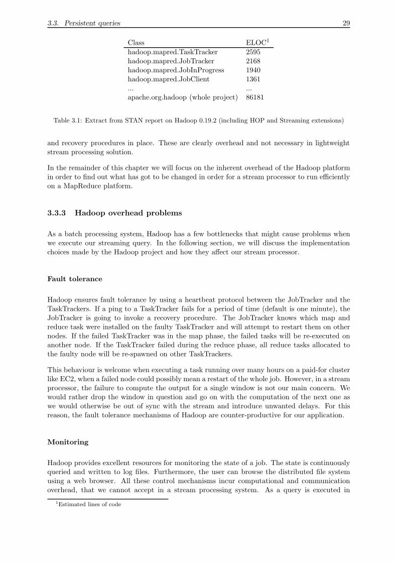
3.3. Persistent queries 29
Class ELOC1
hadoop.mapred.TaskTracker 2595hadoop.mapred.JobTracker 2168hadoop.mapred.JobInProgress 1940hadoop.mapred.JobClient 1361... ...apache.org.hadoop (whole project) 86181
Table 3.1: Extract from STAN report on Hadoop 0.19.2 (including HOP and Streaming extensions)
and recovery procedures in place. These are clearly overhead and not necessary in lightweightstream processing solution.
In the remainder of this chapter we will focus on the inherent overhead of the Hadoop platformin order to find out what has got to be changed in order for a stream processor to run efficientlyon a MapReduce platform.
3.3.3 Hadoop overhead problems
As a batch processing system, Hadoop has a few bottlenecks that might cause problems whenwe execute our streaming query. In the following section, we will discuss the implementationchoices made by the Hadoop project and how they affect our stream processor.
Fault tolerance
Hadoop ensures fault tolerance by using a heartbeat protocol between the JobTracker and theTaskTrackers. If a ping to a TaskTracker fails for a period of time (default is one minute), theJobTracker is going to invoke a recovery procedure. The JobTracker knows which map andreduce task were installed on the faulty TaskTracker and will attempt to restart them on othernodes. If the failed TaskTracker was in the map phase, the failed tasks will be re-executed onanother node. If the TaskTracker failed during the reduce phase, all reduce tasks allocated tothe faulty node will be re-spawned on other TaskTrackers.
This behaviour is welcome when executing a task running over many hours on a paid-for clusterlike EC2, when a failed node could possibly mean a restart of the whole job. However, in a streamprocessor, the failure to compute the output for a single window is not our main concern. Wewould rather drop the window in question and go on with the computation of the next one aswe would otherwise be out of sync with the stream and introduce unwanted delays. For thisreason, the fault tolerance mechanisms of Hadoop are counter-productive for our application.
Monitoring
Hadoop provides excellent resources for monitoring the state of a job. The state is continuouslyqueried and written to log files. Furthermore, the user can browse the distributed file systemusing a web browser. All these control mechanisms incur computational and communicationoverhead, that we cannot accept in a stream processing system. As a query is executed in
1Estimated lines of code
30 Chapter 3. Stream Processing With Hadoop
seconds, or milliseconds, we do not need any information on its completion. This informationcan be gathered by the client software.
The distributed file system is not envisaged to play a role in our stream processing system.Therefore, any overhead due to its operation has to be deemed unnecessary. We will discussthe impact of the remnants of the distributed file system in the next section. At this point wemust conclude that the monitoring as done by the Hadoop framework run against our ideas ofa stream processing system.
Interoperability
Hadoop allows running non-Java code instead of the mapper and reducer functions. This featureis accessed using the Hadoop “Streaming” component - which unfortunately does not bear anyrelation to the concepts discussed in this report. Ensuring compatibility with other languagesincurs overhead penalty on the start up of jobs and is likely to interfere with our low latencyguarantee.
Another aspect of compatibility is the fact that even though we can remove the distributed filesystem from the data processing stage, we cannot entirely drop it due to the fact that it is alsoused as a communication medium between the JobTracker and TaskTrackers for exchanging con-figuration settings and the MapReduce code. Changes to the distributed file system architectureare therefore only going to be possible with a near complete re-write of the Hadoop code base.However, accepting the overhead of the distributed file system for these is difficult to justifywhen we want to optimise the system for minimum delay. We must thus conclude that it willbe a major obstacle in using the Hadoop framework for stream processing applications.
Automatic scaling
Hadoop’s automatic scaling of map and reduce tasks is not build for the data common in streamprocessing systems. A typical window in our financial data set contains only 10,000 tuples andis worth about 800 kilobytes of data. The scaling process in Hadoop is relatively coarse-grainedand will thus result in queries where only a single TaskTracker is utilised. The problem withthe standard allocation is that it is exactly what the Hadoop creators have found to deliverthe best balance taking into account the overhead from the monitoring and fault toleranceprocedures mentioned above. Significantly lowering the split size in our model is likely to resultin a slowdown rather than a speedup. This could only be improved by increasing the complexityof the map and reduce tasks. The MapReduce approach is to split more complicated tasksinto multiple chained MapReduce jobs. This, however, goes against our idea of decreasing theoverhead.
JVM management
Somewhat linked to Hadoop’s scaling mechanism is its management of JVMs2. With the defaultsetting, Hadoop starts a new JVM for every task. A configuration parameter can be used toenable re-usage of JVMs for multiple tasks. However, JVMs are still spawned with every newjob submitted to the JobTracker. This introduces a considerable non-deterministic overhead. Ina stream processing system, the execution of a query must usually be completed in a fraction ofthe time needed to spawn a new JVM. However, as the JVMs are central to the design of the
2Java Virtual Machine
3.4. Lessons learnt 31
Hadoop framework, it is again difficult to remove them without upsetting the other componentsof the system.
3.4 Lessons learnt
The extension of Hadoop has shown us that it is possible to use a MapReduce system to runstreaming queries. However, the legacy of the batch processing framework is to great to efficientlyimplement a stream processor on top of the Hadoop framework. In order to install persistentqueries, that run without the overhead of the distributed file system and Hadoop’s monitoringand recovery facilities, we would have to completely re-write the core of the Hadoop framework.As the whole framework is build on the idea of distributing all data by utilising the distributedfile system, we have opted for another solution. In the next chapter we will show how wehave used the lessons learnt from implementing stream processing on Hadoop to build our owndistributed MapReduce stream processor.

32 Chapter 3. Stream Processing With Hadoop
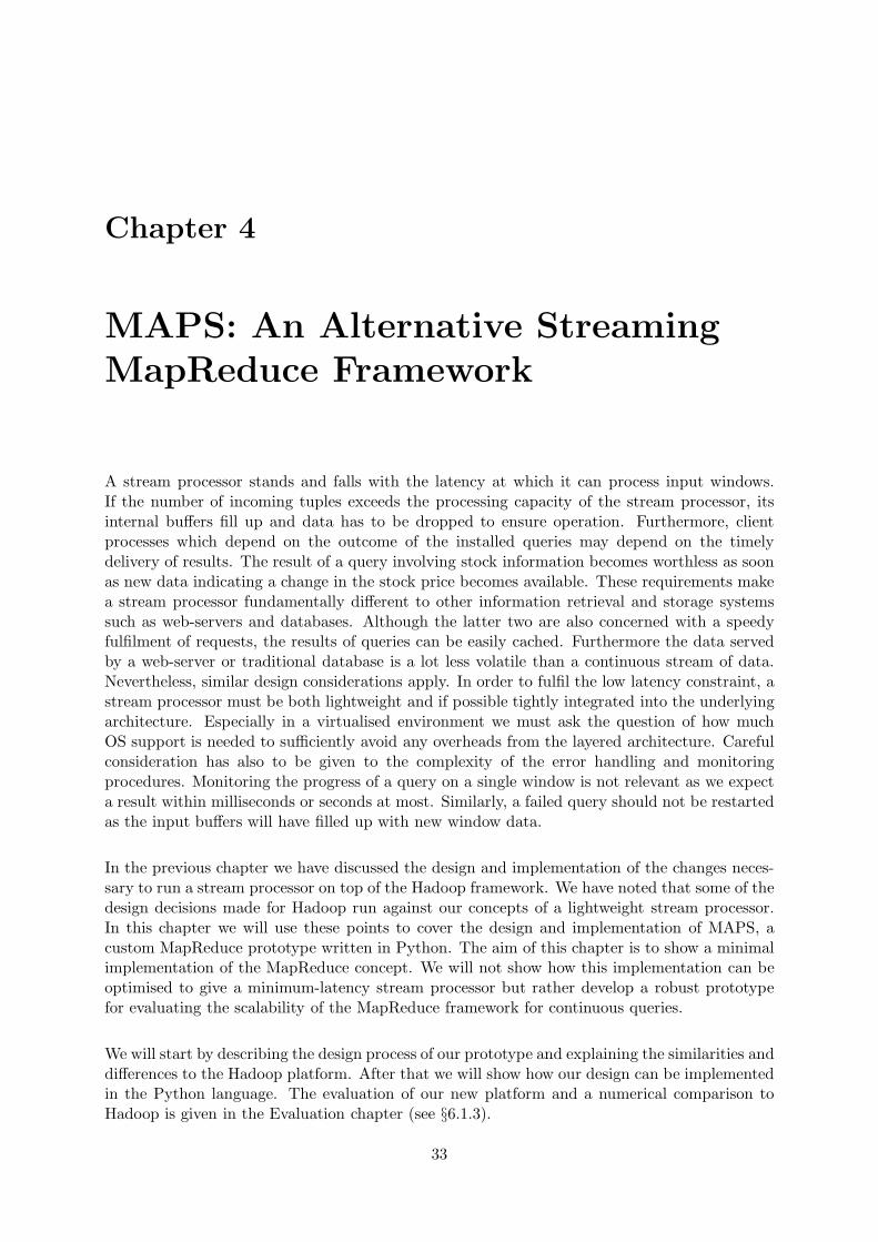
Chapter 4
MAPS: An Alternative StreamingMapReduce Framework
A stream processor stands and falls with the latency at which it can process input windows.If the number of incoming tuples exceeds the processing capacity of the stream processor, itsinternal buffers fill up and data has to be dropped to ensure operation. Furthermore, clientprocesses which depend on the outcome of the installed queries may depend on the timelydelivery of results. The result of a query involving stock information becomes worthless as soonas new data indicating a change in the stock price becomes available. These requirements makea stream processor fundamentally different to other information retrieval and storage systemssuch as web-servers and databases. Although the latter two are also concerned with a speedyfulfilment of requests, the results of queries can be easily cached. Furthermore the data servedby a web-server or traditional database is a lot less volatile than a continuous stream of data.Nevertheless, similar design considerations apply. In order to fulfil the low latency constraint, astream processor must be both lightweight and if possible tightly integrated into the underlyingarchitecture. Especially in a virtualised environment we must ask the question of how muchOS support is needed to sufficiently avoid any overheads from the layered architecture. Carefulconsideration has also to be given to the complexity of the error handling and monitoringprocedures. Monitoring the progress of a query on a single window is not relevant as we expecta result within milliseconds or seconds at most. Similarly, a failed query should not be restartedas the input buffers will have filled up with new window data.
In the previous chapter we have discussed the design and implementation of the changes neces-sary to run a stream processor on top of the Hadoop framework. We have noted that some of thedesign decisions made for Hadoop run against our concepts of a lightweight stream processor.In this chapter we will use these points to cover the design and implementation of MAPS, acustom MapReduce prototype written in Python. The aim of this chapter is to show a minimalimplementation of the MapReduce concept. We will not show how this implementation can beoptimised to give a minimum-latency stream processor but rather develop a robust prototypefor evaluating the scalability of the MapReduce framework for continuous queries.
We will start by describing the design process of our prototype and explaining the similarities anddifferences to the Hadoop platform. After that we will show how our design can be implementedin the Python language. The evaluation of our new platform and a numerical comparison toHadoop is given in the Evaluation chapter (see §6.1.3).
33
34 Chapter 4. MAPS: An Alternative Streaming MapReduce Framework
4.1 Motivation for Python as implementation language
Python cannot be regarded as being among the fastest programming languages in use today. Itis not even one of the faster interpreted languages. In fact, its performance is quite dismal whencompared to code compiled in C or even Java1. Nevertheless, it makes a lot of practical sense toimplement our MapReduce prototype in Python. An obvious point is the ease of developmentand the ability to quickly change the structure of the framework to evaluate alternative ap-proaches. It is very straightforward to exchange a module for another without having to worrystrict type hierarchies. Of course this might result in a run time error every now and then, butfor a system that is merely designed to evaluate a concept, this is acceptable. This is even lessof a problem as small modules can be quickly tested and deployed without having to implementthe whole application - a reason that is further aided by the fact that no compilation is needed toexecute the code. Python gives us a simple way to express the parts of the system that matter.Whereas in Java we would need generics to express the fact that different formats are possible forkey/value pairs, the dynamical type system in Python relieves us of this task. We are thus ableto focus on the control flow among the modules on the master and slave nodes without having toworry much about the format of the data exchanged. Above all other reasons, however, we havechosen Python for its proximity to the functional programming paradigm behind MapReduce.It makes sense to operate on lists rather than arrays when we discuss map and reduce functions.In the background section, we have discussed how languages like Pig and Sawzall (§2.2.2) wereintroduced to simply the developer’s task of writing MapReduce jobs. We feel that there is noneed for any of these if queries can be expressed in functional languages whose concepts lie atthe heart of MapReduce. Last but not least we wish to conclude this discussion by highlightinga quote from Google’s Sawzall paper [34]:
It may seem paradoxical to use an interpreted language in a high-throughput en-vironment, but we have found that the CPU time is rarely the limiting factor; theexpressiveness of the language means that most programs are small and spend mostof their time in I/O and native run-time code.
As the paper suggests, the complexity of our MapReduce framework lies not within its imple-mentation but rather with the choices made with regards to data distribution, load balancingand inter-process communication. Most time-critical libraries exhibited by the Python languageare written in C and do therefore merely involve a small marshaling overhead.
4.2 Design decisions
When designing our MAPS prototype we will focus on rebuilding the essential parts of theHadoop MapReduce system while leaving the non-essential overhead out. We will be re-implementing the core MapReduce logic and forgoing any sort of reporting and advanced errorhandling. For a discussion on the overheads of the Hadoop MapReduce implementation withregards to stream processing consult the previous chapter.
To honour Hadoop’s division into JobTrackers and TaskTrackers, we will split the design into twoparts. First we will discuss the requirements for our master node, containing the StreamServerand the job logic. Then we will go on to describe the implementation of our slave or workernodes. The master node will handle the incoming data and the load balancing over the worker
1http://shootout.alioth.debian.org/u32/benchmark.php?test=nbody&lang=all
4.2. Design decisions 35
nodes. It will further deal with the addition and removal of slave nodes. There will be noprovision for re-starting failed jobs. All the communication with the client is done through themaster node. The worker nodes contain merely the logic needed to run the map and reducefunctions and to participate in the distributed sort in between the two phases.
4.2.1 Role of the JobTracker
Polling vs central allocation of input splits
In Hadoop, the role of the JobTracker is merely to accept incoming jobs, to distribute them overthe TaskTrackers and to provide accounting information to the calling process. Even thoughthe JobTracker is still somewhat involved in a mediating role, it is not directly involved in thecomputation of the results. The job is set up using the JobClient and then send to the JobTrackerfor distribution. Neither class is directly involved in the gathering of input data, the processing ofintermediate data and the output of the final result. In Hadoop, the data source is completelydecoupled from the actual computation. This has allowed us to quickly extend the existingparadigm to allow streaming queries. However, it has also introduced additional overhead dueto the introduction of additional proxies to connect the InputReaders and OutputReaders to theStreamServer. The upside of this distribution of control is an increased parallelism in the dataallocation to the TaskTrackers. The downside is additional control logic in both the StreamServercomponent and the TaskTrackers. For our design, we have chosen to slightly modify the roleof the JobTracker. As shown in Figure 4.2, the JobTracker now deals with the splitting of theinput stream. The QueryHandler sub-module of the JobTracker then allocates the splits to theTaskTrackers and calls their map and reduce functions.
Query installation
Instead of the TaskTrackers polling the JobTracker for new tasks, we have chosen to push thequery to all available TaskTrackers from the JobTracker. We have chosen this option as we aredealing with continuous queries. It is unlikely that a query is changed during the run time ofour stream processor.
When we spawn a new TaskTracker, it remains idle until it receives a request from a JobTracker.The first request by the JobTracker is a call to assert that the TaskTracker is live. It will thenattempt to move the code for the map and reduce functions over the network and install themwithin the TaskTracker. This setup must take place before the first window arrives on the streamprocessor. We do not at this stage plan to introduce functionality that enables changing thequeries in a running system. However, adding a new vanilla TaskTracker to the running systemshould cause the JobTracker to install the query on this node to make it available for processingas the next window comes in.
Query validation
Ideally, the JobTracker should validate the query before installing it on the TaskTrackers. Themap and reduce function must fit the interface with the TaskTracker (i.e. accept key/value pairs)and each other (i.e. provide compatible key/value pairs). This concept is shown in Figure 4.1.As we have chosen not to implement any error handling during the execution of queries, it isparamount to make sure that only valid queries are installed on the TaskTrackers in the first
36 Chapter 4. MAPS: An Alternative Streaming MapReduce Framework
Figure 4.1: Query validation. A functions have to fit to their partner and the framework.
place. To achieve this, the JobTracker checks if the supplied code correctly defines the mapperand reduce functions as required by the TaskTrackers.
4.2.2 Role of the TaskTrackers
A TaskTracker’s main responsibility in our architecture is to compute the results for the appli-cation of the map and reduce on its input split. In addition, it is involved in the partitioningof the results for the reduce phase by sorting the output of its map function. However, theTaskTracker is always passive in its behaviour. The query and its invocations are pushed fromtasks in the JobTracker. The TaskTrackers contain no error handling and expect the query fromthe JobTracker to have been validated. As their map and reduce tasks are invoked from theJobTracker, they are also oblivious to the structure of the map reduce process. They are merelywork horses, designed to quickly return a result to the master for processing.
4.2.3 Possible extensions
The system is designed to easily cope with additions such as a variation in which the masternode handles the map tasks as well. This could be interesting when there is a big discrepancybetween the work done during the map and reduce phases. This shall, however, not be partof our original design as distributing the input data helps us to conduct the necessary sortin a distributed merge-sort fashion. Currently, we have only installed a single query on theTaskTrackers. The architecture can be easily extended to allow for multiple, pipelined queries.This can be interesting when a single MapReduce task is not expressive enough anymore. Wehave ignored this for now due to the added overhead in communication. In Chapter 6, we willdiscuss the parallel overhead in detail.
4.3 Components to be implemented
In this section we will describe the components which need to be implemented for our MAPSframework. Figure 4.2 gives an overview of the components involved in a complete MapReducecycle. The JobTracker handles the distribution of the query. The QueryHandler is a subordinateof the JobTracker which deals with creating the input splits and connecting to the TaskTrackersto spawn the map functions. The OutputCollector takes the partial lists from the mappers and
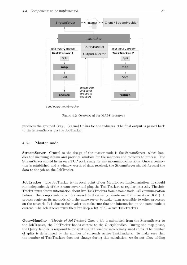
4.3. Components to be implemented 37
Figure 4.2: Overview of our MAPS prototype
produces the grouped (key, [value]) pairs for the reducers. The final output is passed backto the StreamServer via the JobTracker.
4.3.1 Master node
StreamServer Central to the design of the master node is the StreamServer, which han-dles the incoming stream and provides windows for the mappers and reducers to process. TheStreamServer should listen on a TCP port, ready for any incoming connections. Once a connec-tion is established and a window worth of data received, the StreamServer should forward thedata to the job on the JobTracker.
JobTracker The JobTracker is the focal point of our MapReduce implementation. It shouldrun independently of the stream server and ping the TaskTrackers at regular intervals. The Job-Tracker must obtain information about live TaskTrackers from a name node. All communicationbetween the components of our framework is done using remote method invocation (RMI). Aprocess registers its methods with the name server to make them accessible to other processeson the network. It is due to the invoker to make sure that the information on the name node iscurrent. The JobTracker must therefore keep a list of all active TaskTrackers.
QueryHandler (Module of JobTracker) Once a job is submitted from the StreamServer tothe JobTracker, the JobTracker hands control to the QueryHandler. During the map phase,the QueryHandler is responsible for splitting the window into equally sized splits. The numberof splits is determined by the number of currently active TaskTrackers. To make sure thatthe number of TaskTrackers does not change during this calculation, we do not allow adding
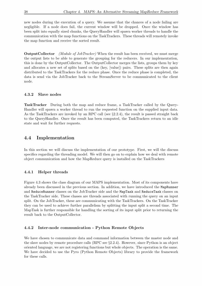
38 Chapter 4. MAPS: An Alternative Streaming MapReduce Framework
new nodes during the execution of a query. We assume that the chances of a node failing arenegligible. If a node does fail, the current window will be dropped. Once the window hasbeen split into equally sized chunks, the QueryHandler will spawn worker threads to handle thecommunication with the map functions on the TaskTrackers. These threads will remotely invokethe map function and receive the sorted result.
OutputCollector (Module of JobTracker) When the result has been received, we must mergethe output lists to be able to generate the grouping for the reducers. In our implementation,this is done by the OutputCollector. The OutputCollector merges the lists, groups them by keyand allocates a new set of splits based on the (key, [value]) pairs. These splits are then againdistributed to the TaskTrackers for the reduce phase. Once the reduce phase is completed, thedata is send via the JobTracker back to the StreamServer to be communicated to the clientnode.
4.3.2 Slave nodes
TaskTracker During both the map and reduce frame, a TaskTracker called by the Query-Handler will spawn a worker thread to run the requested function on the supplied input data.As the TaskTrackers are invoked by an RPC call (see §2.2.4), the result is passed straight backto the QueryHandler. Once the result has been computed, the TaskTrackers return to an idlestate and wait for further requests.
4.4 Implementation
In this section we will discuss the implementation of our prototype. First, we will the discussspecifics regarding the threading model. We will then go on to explain how we deal with remoteobject communication and how the MapReduce query is installed on the TaskTrackers
4.4.1 Helper threads
Figure 4.3 shows the class diagram of our MAPS implementation. Most of its components havealready been discussed in the previous section. In addition, we have introduced the MapRunner
and ReduceRunner classes on the JobTracker side and the MapTask and ReduceTask classes onthe TaskTracker side. These classes are threads associated with running the query on an inputsplit. On the JobTracker, these are communicating with the TaskTrackers. On the TaskTrackerthey can be used to achieve further parallelism by splitting the input split a second time. TheMapTask is further responsible for handling the sorting of its input split prior to returning theresult back to the OutputCollector.
4.4.2 Inter-node communication - Python Remote Objects
We have chosen to communicate data and command information between the master node andthe slave nodes by remote procedure calls (RPC see §2.2.4). However, since Python is an objectoriented language, we are not registering functions but whole objects. The operation is the same.We have decided to use the Pyro (Python Remote Objects) library to provide the frameworkfor these calls.
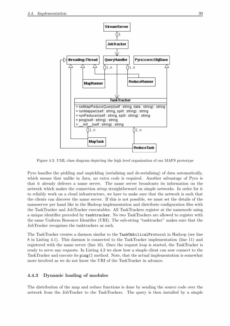
4.4. Implementation 39
Figure 4.3: UML class diagram depicting the high level organisation of our MAPS prototype
Pyro handles the pickling and unpickling (serialising and de-serialising) of data automatically,which means that unlike in Java, no extra code is required. Another advantage of Pyro isthat it already delivers a name server. The name server broadcasts its information on thenetwork which makes the connection setup straightforward on simple networks. In order for itto reliably work on a cloud infrastructure, we have to make sure that the network is such thatthe clients can discover the name server. If this is not possible, we must set the details of thenameserver per hand like in the Hadoop implementation and distribute configuration files withthe TaskTracker and JobTracker executables. All TaskTrackers register at the namenode usinga unique identifier preceded by tasktracker. No two TaskTrackers are allowed to register withthe same Uniform Resource Identifier (URI). The sub-string “tasktracker” makes sure that theJobTracker recognises the tasktrackers as such.
The TaskTracker creates a daemon similar to the TaskUmbilicalProtocol in Hadoop (see line8 in Listing 4.1). This daemon is connected to the TaskTracker implementation (line 11) andregistered with the name server (line 10). Once the request loop is started, the TaskTracker isready to serve any requests. In Listing 4.2 we show how a simple client can now connect to theTaskTracker and execute its ping() method. Note, that the actual implementation is somewhatmore involved as we do not know the URI of the TaskTracker in advance.
4.4.3 Dynamic loading of modules
The distribution of the map and reduce functions is done by sending the source code over thenetwork from the JobTracker to the TaskTrackers. The query is then installed by a simple
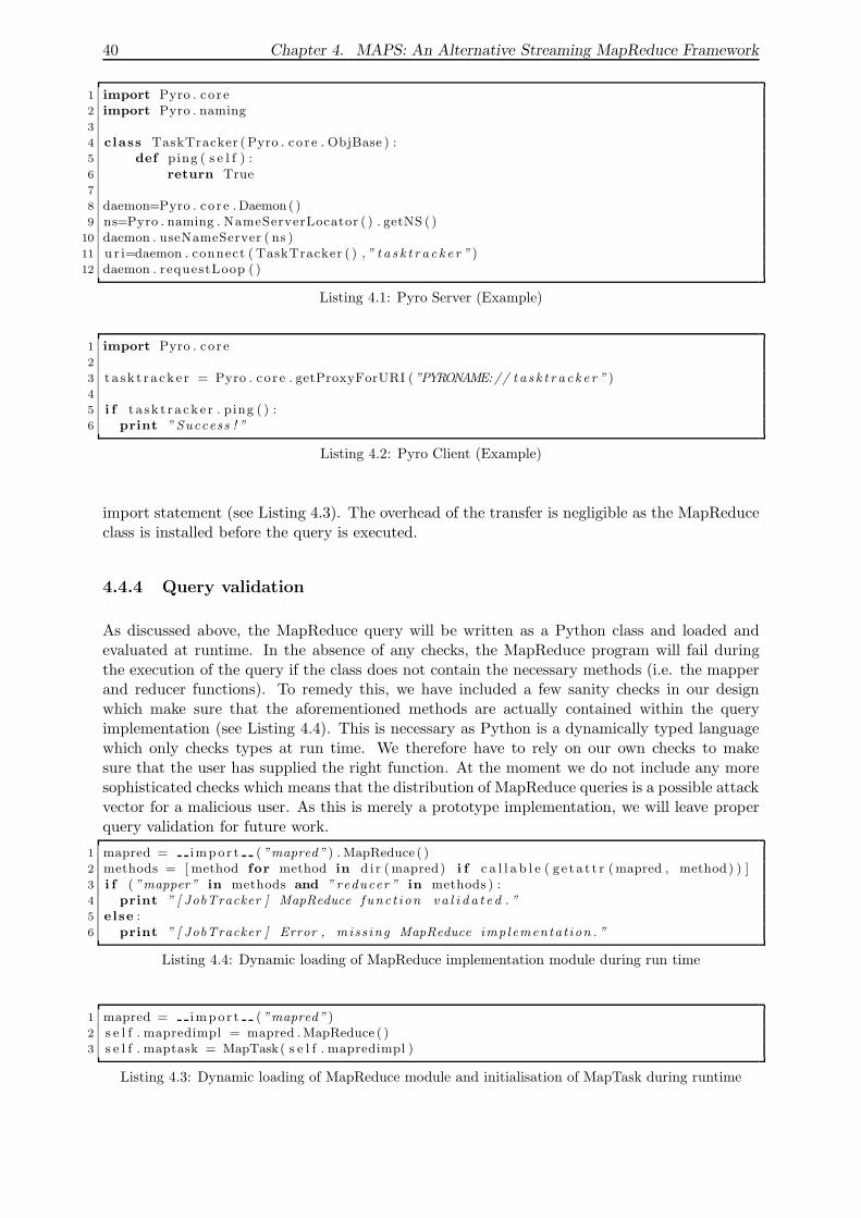
40 Chapter 4. MAPS: An Alternative Streaming MapReduce Framework
1 import Pyro . core2 import Pyro . naming3
4 class TaskTracker ( Pyro . core . ObjBase ) :5 def ping ( s e l f ) :6 return True7
8 daemon=Pyro . core .Daemon ( )9 ns=Pyro . naming . NameServerLocator ( ) . getNS ( )
10 daemon . useNameServer ( ns )11 u r i=daemon . connect ( TaskTracker ( ) ,” t a s k t r a c k e r ” )12 daemon . requestLoop ( )
Listing 4.1: Pyro Server (Example)
1 import Pyro . core2
3 t a sk t r a ck e r = Pyro . core . getProxyForURI (”PYRONAME:// t a s k t r a c k e r ” )4
5 i f t a sk t r a ck e r . ping ( ) :6 print ” Success ! ”
Listing 4.2: Pyro Client (Example)
import statement (see Listing 4.3). The overhead of the transfer is negligible as the MapReduceclass is installed before the query is executed.
4.4.4 Query validation
As discussed above, the MapReduce query will be written as a Python class and loaded andevaluated at runtime. In the absence of any checks, the MapReduce program will fail duringthe execution of the query if the class does not contain the necessary methods (i.e. the mapperand reducer functions). To remedy this, we have included a few sanity checks in our designwhich make sure that the aforementioned methods are actually contained within the queryimplementation (see Listing 4.4). This is necessary as Python is a dynamically typed languagewhich only checks types at run time. We therefore have to rely on our own checks to makesure that the user has supplied the right function. At the moment we do not include any moresophisticated checks which means that the distribution of MapReduce queries is a possible attackvector for a malicious user. As this is merely a prototype implementation, we will leave properquery validation for future work.
1 mapred = impor t (”mapred” ) . MapReduce ( )2 methods = [ method for method in d i r (mapred) i f c a l l a b l e ( g e t a t t r (mapred , method) ) ]3 i f (”mapper” in methods and ” reducer ” in methods ) :4 print ” [ JobTracker ] MapReduce func t i on v a l i d a t e d . ”5 else :6 print ” [ JobTracker ] Error , miss ing MapReduce implementat ion . ”
Listing 4.4: Dynamic loading of MapReduce implementation module during run time
1 mapred = impor t (”mapred” )2 s e l f . mapredimpl = mapred . MapReduce ( )3 s e l f . maptask = MapTask( s e l f . mapredimpl )
Listing 4.3: Dynamic loading of MapReduce module and initialisation of MapTask during runtime
4.5. Discussion 41
4.5 Discussion
When we designed MAPS, the goal was to remove some of the overhead introduced by theHadoop framework (§3.3.3). Our design is not based on a distributed file system while stillenabling the user to distribute the map and reduce functions through a single point of entry.We have compromised on speed by using remote procedure calls, staying true to the Hadoopframework. For a more efficient implementation we would consider use a technology like MPI [26]for distributing the data.
Besides the communication overhead, we acknowledge that the choice of the implementationlanguage has reduced the efficiency of our stream processor. The significance of this overheadis set into perspective when we compare the run time of our custom implementation to Hadoopin Chapter 6.
The evaluation must further show if our decision to centralise the distribution of input splitshas worked. We deem it to be unnecessary to have the TaskTrackers polling for new data. InHadoop, one of the reasons why this is done is because idle TaskTrackers can do speculativeexecution of tasks, thereby avoiding the situation in which all TaskTrackers wait for the outputof a single one. The MapReduce algorithm has to synchronise the TaskTrackers in betweenthe map and reduce phases to do the grouping. With speculative execution, the impact of anunresponsive TaskTracker could be remedied. In our implementation we will immediately see ifa TaskTracker is unresponsive. The window is dropped and the TaskTracker removed from thepool for the next iteration. Speculative execution only introduces an additional overhead thatwe cannot be prepared to take if we want to achieve a low latency response.

42 Chapter 4. MAPS: An Alternative Streaming MapReduce Framework
Chapter 5
Load Balancing Into The Cloud
The second part of our project focuses on a solution to enable a local stream processor to utilisethe cloud infrastructure to guarantee a latency bound on the computation time. In this chapterwe will first describe the design and implementation of simple local MapReduce style streamprocessor. We will then go on to design two load balancing strategies. First we will consideran always-on approach in which the load is balanced between the local node and the cloud inorder to achieve a higher throughput overall. The always-on approach is not economical. Infact, it raises the question why we would not move all processing to the cloud in the first place,thereby eliminating the need for both the load balancer and the local processor. However, thealways-on load balancer can be used to find the best split between cloud processor and the localnode with respect to network bandwidth and the scalability of the query. A higher bandwidthbetween the load balancer and the cloud or a more complex query will result in more windowsbeing processed by the cloud.
Building on these ideas we will introduce an alternative approach. In adaptive-load balancing,the cloud is used as a backup system to deal with peaks in the load. We expect the local streamprocessor to deal with the stream most of the time. However, when the incoming data exceedsa certain rate, it has to begin to drop windows. At this point the adaptive load balancingalgorithm should begin to move computation to the cloud, thereby lowering the number ofwindows dropped while ensuring the latency constraints are met. By only utilising the cloudinfrastructure to support the local processor on-demand, we can keep costs at a minimum.
5.1 Local stream processor
In the last chapter, we have described a distributed MapReduce framework written in Python.This framework may be simplified to run on a single node. It is clear that any of the otherstream processors described in the background section are equally applicable here. However, animplementation similar to our cloud architecture will result in more seamless load balancing aswe can standardise the input and output formats. In fact, we could simply re-use MAPS anddeploy it on a single node. Performance figures for this approach are given in the next chapter.We have chosen to simplify our existing Python solution to accommodate the need for the loadbalancer to run on the same node. We shall now describe how we simplified the design and theeffects of these changes on the processing of a single MapReduce query.
43
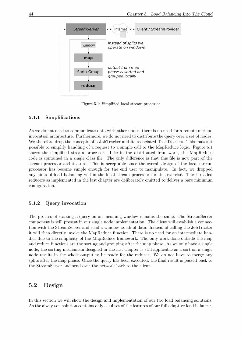
44 Chapter 5. Load Balancing Into The Cloud
Figure 5.1: Simplified local stream processor
5.1.1 Simplifications
As we do not need to communicate data with other nodes, there is no need for a remote methodinvocation architecture. Furthermore, we do not need to distribute the query over a set of nodes.We therefore drop the concepts of a JobTracker and its associated TaskTrackers. This makes itpossible to simplify handling of a request to a simple call to the MapReduce logic. Figure 5.1shows the simplified stream processor. Like in the distributed framework, the MapReducecode is contained in a single class file. The only difference is that this file is now part of thestream processor architecture. This is acceptable since the overall design of the local streamprocessor has become simple enough for the end user to manipulate. In fact, we droppedany hints of load balancing within the local stream processor for this exercise. The threadedreducers as implemented in the last chapter are deliberately omitted to deliver a bare minimumconfiguration.
5.1.2 Query invocation
The process of starting a query on an incoming window remains the same. The StreamServercomponent is still present in our single node implementation. The client will establish a connec-tion with the StreamServer and send a window worth of data. Instead of calling the JobTrackerit will then directly invoke the MapReduce function. There is no need for an intermediate han-dler due to the simplicity of the MapReduce framework. The only work done outside the mapand reduce functions are the sorting and grouping after the map phase. As we only have a singlenode, the sorting mechanism designed in the last chapter is still applicable as a sort on a singlenode results in the whole output to be ready for the reducer. We do not have to merge anysplits after the map phase. Once the query has been executed, the final result is passed back tothe StreamServer and send over the network back to the client.
5.2 Design
In this section we will show the design and implementation of our two load balancing solutions.As the always-on solution contains only a subset of the features of our full adaptive load balancer,
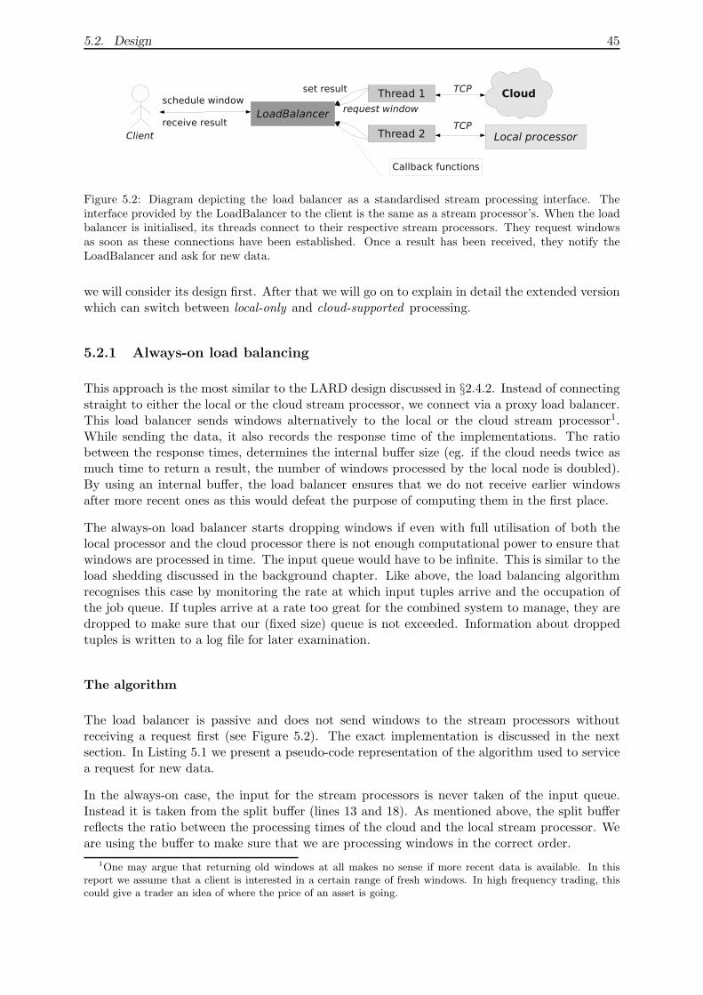
5.2. Design 45
Figure 5.2: Diagram depicting the load balancer as a standardised stream processing interface. Theinterface provided by the LoadBalancer to the client is the same as a stream processor’s. When the loadbalancer is initialised, its threads connect to their respective stream processors. They request windowsas soon as these connections have been established. Once a result has been received, they notify theLoadBalancer and ask for new data.
we will consider its design first. After that we will go on to explain in detail the extended versionwhich can switch between local-only and cloud-supported processing.
5.2.1 Always-on load balancing
This approach is the most similar to the LARD design discussed in §2.4.2. Instead of connectingstraight to either the local or the cloud stream processor, we connect via a proxy load balancer.This load balancer sends windows alternatively to the local or the cloud stream processor1.While sending the data, it also records the response time of the implementations. The ratiobetween the response times, determines the internal buffer size (eg. if the cloud needs twice asmuch time to return a result, the number of windows processed by the local node is doubled).By using an internal buffer, the load balancer ensures that we do not receive earlier windowsafter more recent ones as this would defeat the purpose of computing them in the first place.
The always-on load balancer starts dropping windows if even with full utilisation of both thelocal processor and the cloud processor there is not enough computational power to ensure thatwindows are processed in time. The input queue would have to be infinite. This is similar to theload shedding discussed in the background chapter. Like above, the load balancing algorithmrecognises this case by monitoring the rate at which input tuples arrive and the occupation ofthe job queue. If tuples arrive at a rate too great for the combined system to manage, they aredropped to make sure that our (fixed size) queue is not exceeded. Information about droppedtuples is written to a log file for later examination.
The algorithm
The load balancer is passive and does not send windows to the stream processors withoutreceiving a request first (see Figure 5.2). The exact implementation is discussed in the nextsection. In Listing 5.1 we present a pseudo-code representation of the algorithm used to servicea request for new data.
In the always-on case, the input for the stream processors is never taken of the input queue.Instead it is taken from the split buffer (lines 13 and 18). As mentioned above, the split bufferreflects the ratio between the processing times of the cloud and the local stream processor. Weare using the buffer to make sure that we are processing windows in the correct order.
1One may argue that returning old windows at all makes no sense if more recent data is available. In thisreport we assume that a client is interested in a certain range of fresh windows. In high frequency trading, thiscould give a trader an idea of where the price of an asset is going.
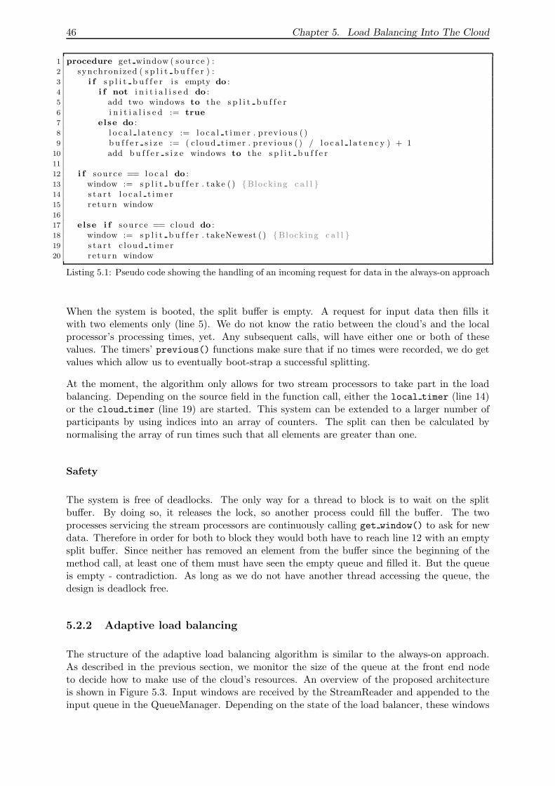
46 Chapter 5. Load Balancing Into The Cloud
1 procedure get window ( source ) :2 synchron ized ( s p l i t b u f f e r ) :3 i f s p l i t b u f f e r i s empty do :4 i f not i n i t i a l i s e d do :5 add two windows to the s p l i t b u f f e r6 i n i t i a l i s e d := true
7 else do :8 l o c a l l a t e n c y := l o c a l t im e r . p rev iou s ( )9 b u f f e r s i z e := ( c loud t imer . p rev iou s ( ) / l o c a l l a t e n c y ) + 1
10 add b u f f e r s i z e windows to the s p l i t b u f f e r11
12 i f sou rce == l o c a l do :13 window := s p l i t b u f f e r . take ( ) {Block ing c a l l }14 s t a r t l o c a l t im e r15 r e tu rn window16
17 else i f sou rce == cloud do :18 window := s p l i t b u f f e r . takeNewest ( ) {Block ing c a l l }19 s t a r t c loud t imer20 r e tu rn window
Listing 5.1: Pseudo code showing the handling of an incoming request for data in the always-on approach
When the system is booted, the split buffer is empty. A request for input data then fills itwith two elements only (line 5). We do not know the ratio between the cloud’s and the localprocessor’s processing times, yet. Any subsequent calls, will have either one or both of thesevalues. The timers’ previous() functions make sure that if no times were recorded, we do getvalues which allow us to eventually boot-strap a successful splitting.
At the moment, the algorithm only allows for two stream processors to take part in the loadbalancing. Depending on the source field in the function call, either the local timer (line 14)or the cloud timer (line 19) are started. This system can be extended to a larger number ofparticipants by using indices into an array of counters. The split can then be calculated bynormalising the array of run times such that all elements are greater than one.
Safety
The system is free of deadlocks. The only way for a thread to block is to wait on the splitbuffer. By doing so, it releases the lock, so another process could fill the buffer. The twoprocesses servicing the stream processors are continuously calling get window() to ask for newdata. Therefore in order for both to block they would both have to reach line 12 with an emptysplit buffer. Since neither has removed an element from the buffer since the beginning of themethod call, at least one of them must have seen the empty queue and filled it. But the queueis empty - contradiction. As long as we do not have another thread accessing the queue, thedesign is deadlock free.
5.2.2 Adaptive load balancing
The structure of the adaptive load balancing algorithm is similar to the always-on approach.As described in the previous section, we monitor the size of the queue at the front end nodeto decide how to make use of the cloud’s resources. An overview of the proposed architectureis shown in Figure 5.3. Input windows are received by the StreamReader and appended to theinput queue in the QueueManager. Depending on the state of the load balancer, these windows
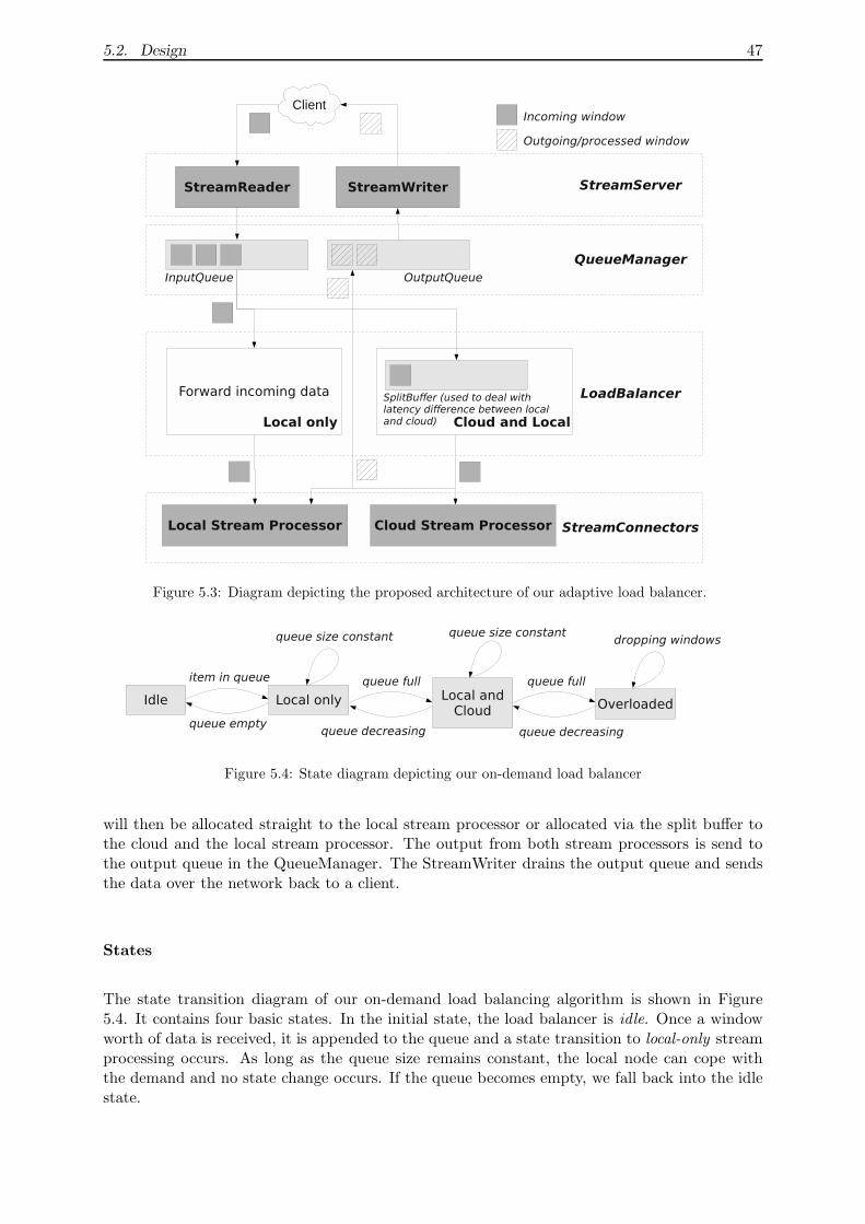
5.2. Design 47
Figure 5.3: Diagram depicting the proposed architecture of our adaptive load balancer.
Figure 5.4: State diagram depicting our on-demand load balancer
will then be allocated straight to the local stream processor or allocated via the split buffer tothe cloud and the local stream processor. The output from both stream processors is send tothe output queue in the QueueManager. The StreamWriter drains the output queue and sendsthe data over the network back to a client.
States
The state transition diagram of our on-demand load balancing algorithm is shown in Figure5.4. It contains four basic states. In the initial state, the load balancer is idle. Once a windowworth of data is received, it is appended to the queue and a state transition to local-only streamprocessing occurs. As long as the queue size remains constant, the local node can cope withthe demand and no state change occurs. If the queue becomes empty, we fall back into the idlestate.
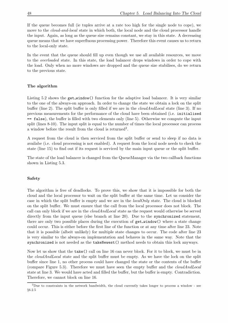
48 Chapter 5. Load Balancing Into The Cloud
If the queue becomes full (ie tuples arrive at a rate too high for the single node to cope), wemove to the cloud-and-local state in which both, the local node and the cloud processor handlethe input. Again, as long as the queue size remains constant, we stay in this state. A decreasingqueue means that we have superfluous processing power. Therefore this event causes us to returnto the local-only state.
In the event that the queue should fill up even though we use all available resources, we moveto the overloaded state. In this state, the load balancer drops windows in order to cope withthe load. Only when no more windows are dropped and the queue size stabilises, do we returnto the previous state.
The algorithm
Listing 5.2 shows the get window() function for the adaptive load balancer. It is very similarto the one of the always-on approach. In order to change the state we obtain a lock on the splitbuffer (line 2). The split buffer is only filled if we are in the cloudAndLocal state (line 3). If noprevious measurements for the performance of the cloud have been obtained (i.e. initialised== false), the buffer is filled with two elements only (line 5). Otherwise we compute the inputsplit (lines 8-10). The input split is equal to the number of times the local processor can processa window before the result from the cloud is returned2.
A request from the cloud is then serviced from the split buffer or send to sleep if no data isavailabe (i.e. cloud processing is not enabled). A request from the local node needs to check thestate (line 15) to find out if its request is serviced by the main input queue or the split buffer.
The state of the load balancer is changed from the QueueManager via the two callback functionsshown in Listing 5.3.
Safety
The algorithm is free of deadlocks. To prove this, we show that it is impossible for both thecloud and the local processor to wait on the split buffer at the same time. Let us consider thecase in which the split buffer is empty and we are in the localOnly state. The cloud is blockedon the split buffer. We must ensure that the call from the local processor does not block. Thecall can only block if we are in the cloudAndLocal state as the request would otherwise be serveddirectly from the input queue (else branch at line 20). Due to the synchronized statement,there are only two possible places during the execution of get window() where a state changecould occur. This is either before the first line of the function or at any time after line 23. Notethat it is possible (albeit unlikely) for multiple state changes to occur. The code after line 23is very similar to the always-on implementation and behaves in the same way. Note that thesynchronized is not needed as the takeNewest() method needs to obtain this lock anyways.
Now let us show that the take() call on line 16 can never block. For it to block, we must be inthe cloudAndLocal state and the split buffer must be empty. As we have the lock on the splitbuffer since line 1, no other process could have changed the state or the contents of the buffer(compare Figure 5.3). Therefore we must have seen the empty buffer and the cloudAndLocalstate at line 3. We would have acted and filled the buffer, but the buffer is empty. Contradiction.Therefore, we cannot block on line 16.
2Due to constraints in the network bandwidth, the cloud currently takes longer to process a window - see§6.2.5
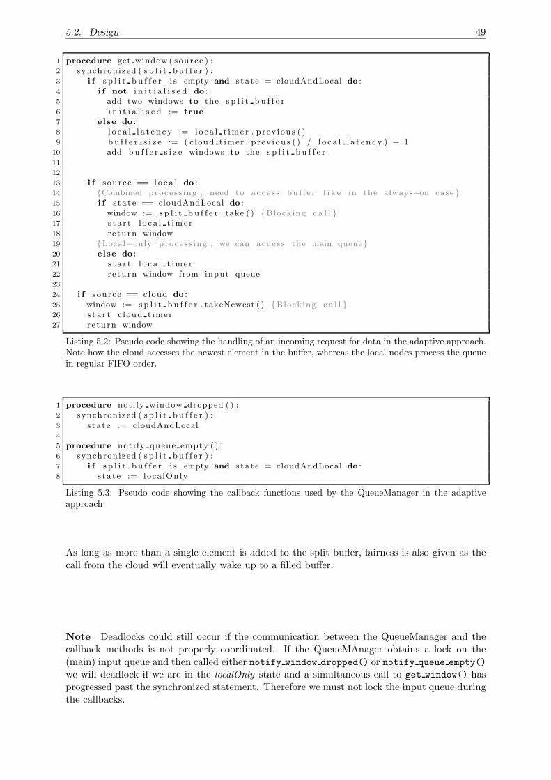
5.2. Design 49
1 procedure get window ( source ) :2 synchron ized ( s p l i t b u f f e r ) :3 i f s p l i t b u f f e r i s empty and s t a t e = cloudAndLocal do :4 i f not i n i t i a l i s e d do :5 add two windows to the s p l i t b u f f e r6 i n i t i a l i s e d := true
7 else do :8 l o c a l l a t e n c y := l o c a l t im e r . p rev iou s ( )9 b u f f e r s i z e := ( c loud t imer . p rev iou s ( ) / l o c a l l a t e n c y ) + 1
10 add b u f f e r s i z e windows to the s p l i t b u f f e r11
12
13 i f sou rce == l o c a l do :14 {Combined proce s s ing , need to ac c e s s bu f f e r l i k e in the always−on case }15 i f s t a t e == cloudAndLocal do :16 window := s p l i t b u f f e r . take ( ) {Block ing c a l l }17 s t a r t l o c a l t im e r18 r e tu rn window19 {Local−only proce s s ing , we can ac c e s s the main queue}20 else do :21 s t a r t l o c a l t im e r22 r e tu rn window from input queue23
24 i f sou rce == cloud do :25 window := s p l i t b u f f e r . takeNewest ( ) {Block ing c a l l }26 s t a r t c loud t imer27 r e tu rn window
Listing 5.2: Pseudo code showing the handling of an incoming request for data in the adaptive approach.Note how the cloud accesses the newest element in the buffer, whereas the local nodes process the queuein regular FIFO order.
1 procedure notify window dropped ( ) :2 synchron ized ( s p l i t b u f f e r ) :3 s t a t e := cloudAndLocal4
5 procedure not i fy queue empty ( ) :6 synchron ized ( s p l i t b u f f e r ) :7 i f s p l i t b u f f e r i s empty and s t a t e = cloudAndLocal do :8 s t a t e := loca lOn ly
Listing 5.3: Pseudo code showing the callback functions used by the QueueManager in the adaptiveapproach
As long as more than a single element is added to the split buffer, fairness is also given as thecall from the cloud will eventually wake up to a filled buffer.
Note Deadlocks could still occur if the communication between the QueueManager and thecallback methods is not properly coordinated. If the QueueMAnager obtains a lock on the(main) input queue and then called either notify window dropped() or notify queue empty()
we will deadlock if we are in the localOnly state and a simultaneous call to get window() hasprogressed past the synchronized statement. Therefore we must not lock the input queue duringthe callbacks.
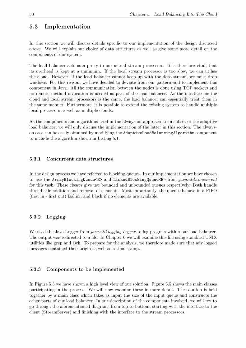
50 Chapter 5. Load Balancing Into The Cloud
5.3 Implementation
In this section we will discuss details specific to our implementation of the design discussedabove. We will explain our choice of data structures as well as give some more detail on thecomponents of our system.
The load balancer acts as a proxy to our actual stream processors. It is therefore vital, thatits overhead is kept at a minimum. If the local stream processor is too slow, we can utilisethe cloud. However, if the load balancer cannot keep up with the data stream, we must dropwindows. For this reason, we have decided to deviate from our pattern and to implement thiscomponent in Java. All the communication between the nodes is done using TCP sockets andno remote method invocation is needed as part of the load balancer. As the interface for thecloud and local stream processors is the same, the load balancer can essentially treat them inthe same manner. Furthermore, it is possible to extend the existing system to handle multiplelocal processors as well as multiple clouds.
As the components and algorithms used in the always-on approach are a subset of the adaptiveload balancer, we will only discuss the implementation of the latter in this section. The always-on case can be easily obtained by modifying the AdaptiveLoadBalancingAlgorithm componentto include the algorithm shown in Listing 5.1.
5.3.1 Concurrent data structures
In the design process we have referred to blocking queues. In our implementation we have chosento use the ArrayBlockingQueue<E> and LinkedBlockingQueue<E> from java.util.concurrentfor this task. These classes give use bounded and unbounded queues respectively. Both handlethread safe addition and removal of elements. Most importantly, the queues behave in a FIFO(first in - first out) fashion and block if no elements are available.
5.3.2 Logging
We used the Java Logger from java.util.logging.Logger to log progress within our load balancer.The output was redirected to a file. In Chapter 6 we will examine this file using standard UNIXutilities like grep and awk. To prepare for the analysis, we therefore made sure that any loggedmessages contained their origin as well as a time stamp.
5.3.3 Components to be implemented
In Figure 5.3 we have shown a high level view of our solution. Figure 5.5 shows the main classesparticipating in the process. We will now examine these in more detail. The solution is heldtogether by a main class which takes as input the size of the input queue and constructs theother parts of our load balancer. In our description of the components involved, we will try togo through the aforementioned diagrams from top to bottom, starting with the interface to theclient (StreamServer) and finishing with the interface to the stream processors.
5.3. Implementation 51
Figure 5.5: Class diagram depicting the organisation of our load balancing solution
StreamServer
The StreamServer component can be compared to its namesake in the Python and Hadoopstream processor implementations. It is responsible for managing the connection to the client.In order to fulfil this task, it creates two threads - StreamReader and StreamWriter - to servethe input and output streams respectively.
StreamReader The StreamReader is a thread which listens for incoming tuples. Once awindow of data has been collected, it is send to the QueueManager. It is the responsibilityof the QueueManager to decide how to deal with it. The StreamReader does not wait on theQueueManager and returns immediately to servicing the input stream.
StreamWriter The StreamWriter is a thread which allows the client to connect on a differentport. We have separated the handling of input and output for the load balancer such that itbecomes possible for the output of the loadbalancer to be forwarded to a different host. Weassume that the originator of the stream is not necessarily the same as the subscriber (eg. astock exchange and a bank respectively). The StreamWriter calls the QueueManager and blockson the OutputQueue if no data is available.
QueueManager
The QueueManager has jurisdiction about the input and output queues. It handles the droppingof windows if the size of the input queue is about to be exceeded. The oldest window is droppedfrom the queue and the new window appended. The QueueManager uses the callback function
52 Chapter 5. Load Balancing Into The Cloud
notify window dropped() defined in the QueueEventsListener interface (see below) to makethe algorithm aware of this event. Likewise, the notify queue empty() callback is used whenthe input queue has been exhausted. This enables the load balancing algorithm to evaluate thepossibility of scaling back to local-only processing. The QueueManager gives the algorithm thepossibility to obtain a single window from the input queue. Alternatively, it is possible to requesta list of n windows. In the latter case, the QueueManager will return min(size(inputQueue), n)windows. This call is used when the algorithm tries to fill its split buffer.
The QueueManager also deals with the output queue. The collect() method from the loadbalancing algorithm is re-directed here. As mentioned above, the output queue is read by theStreamWriter and forwarded back to the client.
LoadBalancingAlgorithm
LoadBalancingAlgorithm is the interface describing the responsibilities of our algorithm. It ex-tends QueueEventsListener, OutputCollector and StreamProvider. The QueueEventsListener
describes callback methods which can be used by the QueueManager to inform the algorithm ifwindows have been dropped or the queue has been drained empty. This information is neededby the LoadBalancingAlgorithm to make decisions about the next state. The OutputCollectorand StreamProvider interfaces are linked to the callbacks from the classes implementing theStreamConnector interface (see below discussion). They allow the stream server to query thealgorithm for windows to process and to contact it with the output data.
LoadCoordinator The LoadCoordinator class connects to the QueueManager and creates theinstance of the load balancing algorithm to deal with the callbacks from the stream processors.It connects the callback from the QueueManager to the LoadBalancingAlgorithm.
AdaptiveLoadBalancingAlgorithm This is a concrete implementation of the LoadBalancingAlgorithm interface and the algorithm shown in Listing 5.2 and the callbacks of Listing 5.3.The state is implemented using an enum type. The internal buffer is constructed from aArrayBlockingQueue<E> as mentioned previously. It is using the WindowDelayTimer customtimer implementation to compute the size of the internal buffer.
WindowDelayTimer The WindowDelayTimer class is used by the load balancing algorithmto get information about the latency of our stream server implementations. When we startprocessing on either the cloud or the local node, we start the timer using its start() method.A call to the stop() method returns the time spent processing. The time is obtained using theSystem.nanoseconds() method. The class further delivers the time previously recorded usingthe previous() method. An average of the last 5 (a different number can be specified in theconstructor) times can be obtained by the average() method. We prefer this to the previous()implementation as it gives us a better estimate on the latency of the next window.
Stream connectors
The StreamConnector interface describes a thread to handle the connection to a stream server.We have two concrete implementations: PersistentStreamConnector and TransientStreamCon-nector. As mentioned previously, these threads connect to the stream server and then call uponthe load balancing algorithm to provide input data.
5.4. Discussion 53
PersistentStreamConnector This class maintains a single connection to the StreamServerof our stream processors (cloud or local). This connection is kept alive for as long as the loadbalancer is running. This is the most efficient way to connect the load balancer to the streamprocessors in a connection-oriented protocol.
TransientStreamConnector This class can be used to connect to a stream processor whichends the connection after the computation of a single window. It automatically re-connects tobe ready for the transmission of the next window.
5.4 Discussion
In this chapter we have shown how to design an adaptive load balancing algorithm to handle thedistribution of work between a local stream processor and the cloud implementations describedin the previous chapters. We have chosen Java as our implementation language to make surethat the overhead from the load balancer is as small as possible. We have deliberately movedthe control flow of load balancing to the stream connectors. Their calls to the get window()
function drive the computation of results. This allows us to extend the algorithm to run onmore than a single cloud and local node.
We have shown how our always-on and adaptive algorithms are safe with respect to deadlocks.It remains to be seen if the coarse locking had an impact on the performance. As we notedduring the discussion of the safety of the adaptive algorithm, we must add at least 2 windowsto the split buffer in order for the cloud to have the chance of getting a window to process. Itwill be interesting to see how the sizes of both the input queue and the split buffer behave.
In the next chapter we will assess the performance of our load balancing solution in regard toits ability to reduce the number of windows dropped as well as its impact on the latency of thecombined system.

54 Chapter 5. Load Balancing Into The Cloud
Chapter 6
Evaluation
In this chapter, we will start by evaluating our MapReduce implementations for stream pro-cessing on a cloud infrastructure. We will be looking at the theoretical foundations of parallelalgorithm design and show measurements for both Hadoop and MAPS.
We will evaluate our two load balancing solutions. First, we will try to understand how we canutilise the cloud’s resources to give an always-on enhancement to the local stream processor.We will then go on to test our dynamic load-balancer and its capabilities to amortise peaks inthe load on the local machine.
Notation
In our evaluation of the algorithms, we will make use of the big-oh notation to provide an upperand lower bound on their sequential and parallel run time. We shall use Θ(g(n)) such that forany f(n) ∈ Θ(g(n)), f is bounded both above and below by g asymptotically. Furthermore, weshall use the following formula to calculate the speedup of a parallel computation, where Sp isthe speedup of the parallel implementation over the sequential one. T1 denotes the time spendby the sequential algorithm. T2 denotes the time spend by the parallel algorithm on p machines.
Sp =T1
Tp
From the above equation, it becomes obvious, that the best possible speedup is Sp = p/(1+pδ),where δ stands for the the communication overhead per processor. We will assume super-linearspeedup is not possible in our implementation. Following from this assumption, we will try toignore where possible, the impact the memory hierachy has on our simulations.
We will measure the efficiency of our parallel/MapReduce implementation by the followingfunction, where p denotes the number of processors:
Ep =Sp
p=
T1
pTp
The efficiency of the parallel algorithm shows how well we utilise the extra resources. Normally,we are not able to obtain a speedup equal to p when using p processors due to δ, the communi-cation overhead per processor. The efficiency measures the fraction of time a processing unit isusefully employed [26].
55
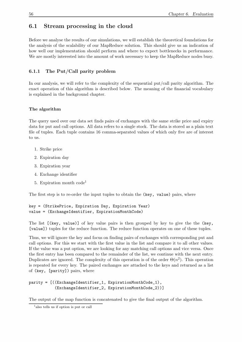
56 Chapter 6. Evaluation
6.1 Stream processing in the cloud
Before we analyse the results of our simulations, we will establish the theoretical foundations forthe analysis of the scalability of our MapReduce solution. This should give us an indication ofhow well our implementation should perform and where to expect bottlenecks in performance.We are mostly interested into the amount of work necessary to keep the MapReduce nodes busy.
6.1.1 The Put/Call parity problem
In our analysis, we will refer to the complexity of the sequential put/call parity algorithm. Theexact operation of this algorithm is described below. The meaning of the financial vocabularyis explained in the background chapter.
The algorithm
The query used over our data set finds pairs of exchanges with the same strike price and expirydata for put and call options. All data refers to a single stock. The data is stored as a plain textfile of tuples. Each tuple contains 16 comma-separated values of which only five are of interestto us.
1. Strike price
2. Expiration day
3. Expiration year
4. Exchange identifier
5. Expiration month code1
The first step is to re-order the input tuples to obtain the (key, value) pairs, where
key = (StrikePrice, Expiration Day, Expiration Year)
value = (ExchangeIdentifier, ExpirationMonthCode)
The list [(key, value)] of key value pairs is then grouped by key to give the the (key,
[value]) tuples for the reduce function. The reduce function operates on one of these tuples.
Thus, we will ignore the key and focus on finding pairs of exchanges with corresponding put andcall options. For this we start with the first value in the list and compare it to all other values.If the value was a put option, we are looking for any matching call options and vice versa. Oncethe first entry has been compared to the remainder of the list, we continue with the next entry.Duplicates are ignored. The complexity of this operation is of the order Θ(n2). This operationis repeated for every key. The paired exchanges are attached to the keys and returned as a listof (key, [parity]) pairs, where
parity = [((ExchangeIdentifier_1, ExpirationMonthCode_1),
(ExchangeIdentifier_2, ExpirationMonthCode_2))]
The output of the map function is concatenated to give the final output of the algorithm.
1also tells us if option is put or call
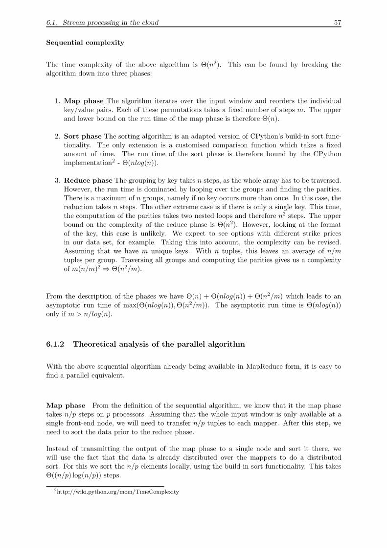
6.1. Stream processing in the cloud 57
Sequential complexity
The time complexity of the above algorithm is Θ(n2). This can be found by breaking thealgorithm down into three phases:
1. Map phase The algorithm iterates over the input window and reorders the individualkey/value pairs. Each of these permutations takes a fixed number of steps m. The upperand lower bound on the run time of the map phase is therefore Θ(n).
2. Sort phase The sorting algorithm is an adapted version of CPython’s build-in sort func-tionality. The only extension is a customised comparison function which takes a fixedamount of time. The run time of the sort phase is therefore bound by the CPythonimplementation2 - Θ(nlog(n)).
3. Reduce phase The grouping by key takes n steps, as the whole array has to be traversed.However, the run time is dominated by looping over the groups and finding the parities.There is a maximum of n groups, namely if no key occurs more than once. In this case, thereduction takes n steps. The other extreme case is if there is only a single key. This time,the computation of the parities takes two nested loops and therefore n2 steps. The upperbound on the complexity of the reduce phase is Θ(n2). However, looking at the formatof the key, this case is unlikely. We expect to see options with different strike pricesin our data set, for example. Taking this into account, the complexity can be revised.Assuming that we have m unique keys. With n tuples, this leaves an average of n/mtuples per group. Traversing all groups and computing the parities gives us a complexityof m(n/m)2 ⇒ Θ(n2/m).
From the description of the phases we have Θ(n) + Θ(nlog(n)) + Θ(n2/m) which leads to anasymptotic run time of max(Θ(nlog(n)),Θ(n2/m)). The asymptotic run time is Θ(nlog(n))only if m > n/log(n).
6.1.2 Theoretical analysis of the parallel algorithm
With the above sequential algorithm already being available in MapReduce form, it is easy tofind a parallel equivalent.
Map phase From the definition of the sequential algorithm, we know that it the map phasetakes n/p steps on p processors. Assuming that the whole input window is only available at asingle front-end node, we will need to transfer n/p tuples to each mapper. After this step, weneed to sort the data prior to the reduce phase.
Instead of transmitting the output of the map phase to a single node and sort it there, wewill use the fact that the data is already distributed over the mappers to do a distributedsort. For this we sort the n/p elements locally, using the build-in sort functionality. This takesΘ((n/p) log(n/p)) steps.
2http://wiki.python.org/moin/TimeComplexity
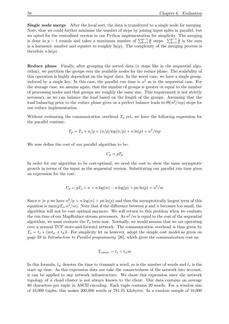
58 Chapter 6. Evaluation
Single node merge After the local sort, the data is transferred to a single node for merging.Note, that we could further minimise the number of steps by joining input splits in parallel, butwe opted for the centralised version in our Python implementation for simplicity. The mergingis done in p − 1 rounds and takes a maximum number of
∑p−1
k=1
nk
steps.∑p−1
k=1
1
kis the sum
is a harmonic number and equates to roughly ln(p). The complexity of the merging process istherefore n ln(p).
Reduce phase Finally, after grouping the sorted data (n steps like in the sequential algo-rithm), we partition the groups over the available nodes for the reduce phase. The scalability ofthis operation is highly dependent on the input data. In the worst case, we have a single group,induced by a single key. In this case, the parallel run time is n2 as in the sequential case. Forthe average case, we assume again, that the number of groups is greater or equal to the numberof processing nodes and that groups are roughly the same size. This requirement is not strictlynecessary, as we can balance the load based on the length of the groups. Assuming that theload balancing prior to the reduce phase gives us a perfect balance leads to Θ(n2/mp) steps forour reduce implementation.
Without evaluating the communication overhead To yet, we have the following expression forthe parallel runtime:
Tp = To + n/p + (n/p) log(n/p) + n ln(p) + n2/mp
We now define the cost of our parallel algorithm to be:
Cp = pTp
In order for our algorithm to be cost-optimal, we need the cost to show the same asymptoticgrowth in terms of the input as the sequential version. Substituting our parallel run time givesan expression for the cost:
Cp = pTo + n + n log(n) − n log(p) + pn ln(p) + n2/m
Since n ≫ p we have n2/p > n log(n) > pn ln(p) and thus the asymptotically largest term of thisequation is max(pTo, n
2/m). Note that if the difference between p and n becomes too small, thealgorithm will not be cost optimal anymore. We will return to this problem when we evaluatethe run time of our MapReduce stream processors. As n2/m is equal to the cost of the sequentialalgorithm, we must evaluate the To term now. Normally, we would assume that we are operatingover a normal TCP store-and-forward network. The communication overhead is thus given byTo = ts + (mtw + th)l. For simplicity let us however, adopt the simple cost model as given onpage 59 in Introduction to Parallel programming [26], which gives the communication cost as:
Tcomm = ts + twm
In this formula, tw denotes the time to transmit a word, m is the number of words and ts is thestart up time. As this expression does not take the connectedness of the network into account,it can be applied to any network infrastructure. We chose this expression since the networktopology of a cloud cluster is not always known to the client. Our data contains on average80 characters per tuple in ASCII encoding. Each tuple contains 20 words. For a window sizeof 10,000 tuples, this makes 200,000 words or 781.25 kilobytes. In a random sample of 10,000
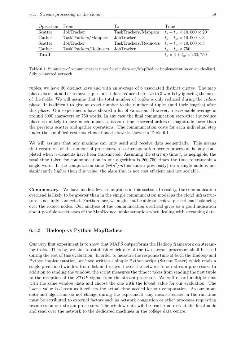
6.1. Stream processing in the cloud 59
Operation From To Time
Scatter JobTracker TaskTrackers/Mappers ts + tw × 10, 000 × 20Gather TaskTrackers/Mappers JobTracker ts + tw × 10, 000 × 3Scatter JobTracker TaskTrackers/Reducers ts + tw × 10, 000 × 3Gather TaskTrackers/Reducers JobTracker ts + tw × 750
Total ts × 4 + tw × 260, 750
Table 6.1: Summary of communication times for our data set/MapReduce implementation on an idealised,fully connected network
tuples, we have 30 distinct keys and with an average of 6 associated distinct quotes. The mapphase does not add or remove tuples but it does reduce their size to 3 words by ignoring the mostof the fields. We will assume that the total number of tuples is only reduced during the reducephase. It is difficult to give an exact number to the number of tuples (and their lengths) afterthis phase. Our experiments have showed a lot of variation. However, a reasonable average isaround 3000 characters or 750 words. In any case the final communication step after the reducephase is unlikely to have much impact as its run time is several orders of magnitude lower thanthe previous scatter and gather operations. The communication costs for each individual stepunder the simplified cost model mentioned above is shown in Table 6.1.
We will assume that any machine can only send and receive data sequentially. This meansthat regardless of the number of processors, a scatter operation over p processors is only com-pleted when n elements have been transmitted. Assuming the start up time ts is negligible, thetotal time taken for communication in our algorithm is 260,750 times the time to transmit asingle word. If the computation time (Θ(n2/m) as shown previously) on a single node is notsignificantly higher than this value, the algorithm is not cost efficient and not scalable.
Commentary We have made a few assumptions in this section. In reality, the communicationoverhead is likely to be greater than in the simple communication model as the cloud infrastruc-ture is not fully connected. Furthermore, we might not be able to achieve perfect load-balancingover the reduce nodes. Our analysis of the communication overhead gives us a good indicationabout possible weaknesses of the MapReduce implementation when dealing with streaming data.
6.1.3 Hadoop vs Python MapReduce
Our very first experiment is to show that MAPS outperforms the Hadoop framework on stream-ing tasks. Thereby, we aim to establish which one of the two stream processors shall be usedduring the rest of this evaluation. In order to measure the response time of both the Hadoop andPython implementation, we have written a simple Python script (StreamTester) which reads asingle predefined window from disk and relays it over the network to our stream processors. Inaddition to sending the window, the script measures the time it takes from sending the first tupleto the reception of the STOP signal from the stream processor. We will record multiple runswith the same window data and choose the one with the lowest value for our evaluation. Thelowest value is chosen as it reflects the actual time needed for our computation. As our inputdata and algorithm do not change during the experiment, any inconsistencies in the run timemust be attributed to external factors such as network congestion or other processes requestingresources on our stream processors. The window data will be read from disk at the local nodeand send over the network to the dedicated machines in the college data centre.
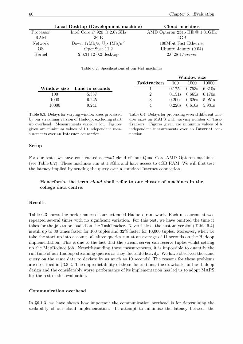
60 Chapter 6. Evaluation
Local Desktop (Development machine) Cloud machines
Processor Intel Core i7 920 @ 2.67GHz AMD Opteron 2346 HE @ 1.81GHzRAM 3GB 4GB
Network Down 17Mb/s, Up 1Mb/s 3 100Mbit Fast EthernetOS OpenSuse 11.2 Ubuntu Jaunty (9.04)
Kernel 2.6.31.12-0.2-desktop 2.6.28-17-server
Table 6.2: Specifications of our test machines
Window size Time in seconds
100 5.3871000 6.22510000 9.241
Table 6.3: Delays for varying window sizes processedby our streaming version of Hadoop, excluding startup overhead. Measurements varied a lot. Figuresgiven are minimum values of 10 independent mea-surements over an Internet connection.
Window sizeTasktrackers 100 1000 10000
1 0.175s 0.753s 6.310s2 0.151s 0.665s 6.170s3 0.200s 0.626s 5.951s4 0.220s 0.610s 5.931s
Table 6.4: Delays for processing several different win-dow sizes on MAPS with varying number of Task-Trackers. Figures given are minimum values of 5independent measurements over an Internet con-nection.
Setup
For our tests, we have constructed a small cloud of four Quad-Core AMD Opteron machines(see Table 6.2). These machines run at 1.8Ghz and have access to 4GB RAM. We will first testthe latency implied by sending the query over a standard Internet connection.
Henceforth, the term cloud shall refer to our cluster of machines in thecollege data centre.
Results
Table 6.3 shows the performance of our extended Hadoop framework. Each measurement wasrepeated several times with no significant variation. For this test, we have omitted the time ittakes for the job to be loaded on the TaskTracker. Nevertheless, the custom version (Table 6.4)is still up to 30 times faster for 100 tuples and 32% faster for 10,000 tuples. Moreover, when wetake the start up into account, all three queries run at an average of 11 seconds on the Hadoopimplementation. This is due to the fact that the stream server can receive tuples whilst settingup the MapReduce job. Notwithstanding these measurements, it is impossible to quantify therun time of our Hadoop streaming queries as they fluctuate heavily. We have observed the samequery on the same data to deviate by as much as 10 seconds! The reasons for these problemsare described in §3.3.3. The unpredictability of these fluctuations, the drawbacks in the Hadoopdesign and the considerably worse performance of its implementation has led us to adopt MAPSfor the rest of this evaluation.
Communication overhead
In §6.1.3, we have shown how important the communication overhead is for determining thescalability of our cloud implementation. In attempt to minimise the latency between the
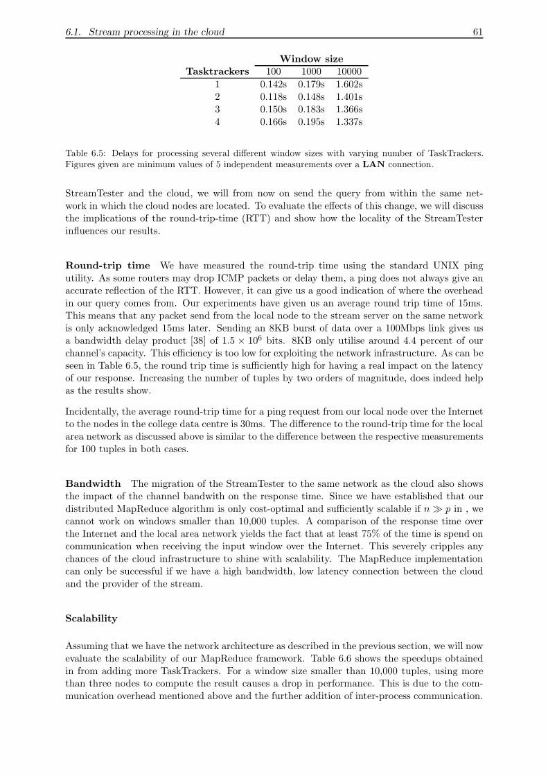
6.1. Stream processing in the cloud 61
Window sizeTasktrackers 100 1000 10000
1 0.142s 0.179s 1.602s2 0.118s 0.148s 1.401s3 0.150s 0.183s 1.366s4 0.166s 0.195s 1.337s
Table 6.5: Delays for processing several different window sizes with varying number of TaskTrackers.Figures given are minimum values of 5 independent measurements over a LAN connection.
StreamTester and the cloud, we will from now on send the query from within the same net-work in which the cloud nodes are located. To evaluate the effects of this change, we will discussthe implications of the round-trip-time (RTT) and show how the locality of the StreamTesterinfluences our results.
Round-trip time We have measured the round-trip time using the standard UNIX pingutility. As some routers may drop ICMP packets or delay them, a ping does not always give anaccurate reflection of the RTT. However, it can give us a good indication of where the overheadin our query comes from. Our experiments have given us an average round trip time of 15ms.This means that any packet send from the local node to the stream server on the same networkis only acknowledged 15ms later. Sending an 8KB burst of data over a 100Mbps link gives usa bandwidth delay product [38] of 1.5 × 106 bits. 8KB only utilise around 4.4 percent of ourchannel’s capacity. This efficiency is too low for exploiting the network infrastructure. As can beseen in Table 6.5, the round trip time is sufficiently high for having a real impact on the latencyof our response. Increasing the number of tuples by two orders of magnitude, does indeed helpas the results show.
Incidentally, the average round-trip time for a ping request from our local node over the Internetto the nodes in the college data centre is 30ms. The difference to the round-trip time for the localarea network as discussed above is similar to the difference between the respective measurementsfor 100 tuples in both cases.
Bandwidth The migration of the StreamTester to the same network as the cloud also showsthe impact of the channel bandwith on the response time. Since we have established that ourdistributed MapReduce algorithm is only cost-optimal and sufficiently scalable if n ≫ p in , wecannot work on windows smaller than 10,000 tuples. A comparison of the response time overthe Internet and the local area network yields the fact that at least 75% of the time is spend oncommunication when receiving the input window over the Internet. This severely cripples anychances of the cloud infrastructure to shine with scalability. The MapReduce implementationcan only be successful if we have a high bandwidth, low latency connection between the cloudand the provider of the stream.
Scalability
Assuming that we have the network architecture as described in the previous section, we will nowevaluate the scalability of our MapReduce framework. Table 6.6 shows the speedups obtainedin from adding more TaskTrackers. For a window size smaller than 10,000 tuples, using morethan three nodes to compute the result causes a drop in performance. This is due to the com-munication overhead mentioned above and the further addition of inter-process communication.
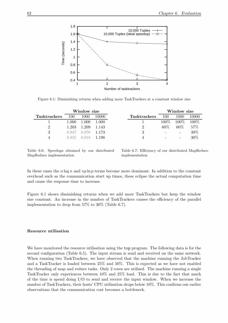
62 Chapter 6. Evaluation
0.4
0.6
0.8
1
1.2
1.4
1.6
1.8
1 2 3 4
Tim
e (s
econ
ds)
Number of tasktrackers
10,000 Tuples10,000 Tuples (ideal speedup)
Figure 6.1: Diminishing returns when adding more TaskTrackers at a constant window size
Window sizeTasktrackers 100 1000 10000
1 1.000 1.000 1.0002 1.203 1.209 1.1433 0.947 0.978 1.1734 0.855 0.918 1.198
Table 6.6: Speedups obtained by our distributedMapReduce implementation
Window sizeTasktrackers 100 1000 10000
1 100% 100% 100%2 60% 60% 57%3 - - 39%4 - - 30%
Table 6.7: Efficiency of our distributed MapReduceimplementation
In these cases the n log n and np ln p terms become more dominant. In addition to the constantoverhead such as the communication start up times, these eclipse the actual computation timeand cause the response time to increase.
Figure 6.1 shows diminishing returns when we add more TaskTrackers but keep the windowsize constant. An increase in the number of TaskTrackers causes the efficiency of the parallelimplementation to drop from 57% to 30% (Table 6.7).
Resource utilisation
We have monitored the resource utilisation using the top program. The following data is for thesecond configuration (Table 6.5). The input stream is send and received on the same network.When running two TaskTrackers, we have observed that the machine running the JobTrackerand a TaskTracker is loaded between 25% and 50%. This is expected as we have not enabledthe threading of map and reduce tasks. Only 2 cores are utilised. The machine running a singleTaskTracker only experiences between 10% and 25% load. This is due to the fact that muchof the time is spend doing I/O to send and receive the input window. When we increase thenumber of TaskTrackers, their hosts’ CPU utilisation drops below 10%. This confirms our earlierobservations that the communication cost becomes a bottleneck.
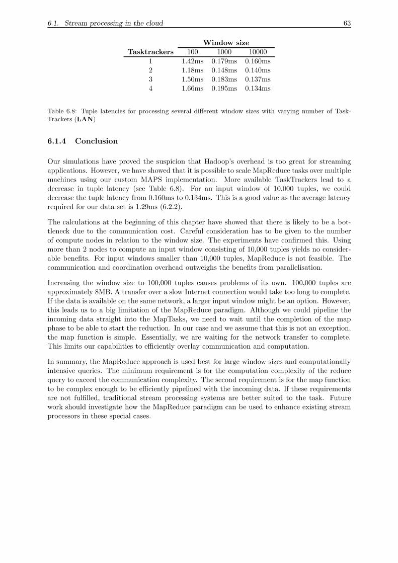
6.1. Stream processing in the cloud 63
Window sizeTasktrackers 100 1000 10000
1 1.42ms 0.179ms 0.160ms2 1.18ms 0.148ms 0.140ms3 1.50ms 0.183ms 0.137ms4 1.66ms 0.195ms 0.134ms
Table 6.8: Tuple latencies for processing several different window sizes with varying number of Task-Trackers (LAN)
6.1.4 Conclusion
Our simulations have proved the suspicion that Hadoop’s overhead is too great for streamingapplications. However, we have showed that it is possible to scale MapReduce tasks over multiplemachines using our custom MAPS implementation. More available TaskTrackers lead to adecrease in tuple latency (see Table 6.8). For an input window of 10,000 tuples, we coulddecrease the tuple latency from 0.160ms to 0.134ms. This is a good value as the average latencyrequired for our data set is 1.29ms (6.2.2).
The calculations at the beginning of this chapter have showed that there is likely to be a bot-tleneck due to the communication cost. Careful consideration has to be given to the numberof compute nodes in relation to the window size. The experiments have confirmed this. Usingmore than 2 nodes to compute an input window consisting of 10,000 tuples yields no consider-able benefits. For input windows smaller than 10,000 tuples, MapReduce is not feasible. Thecommunication and coordination overhead outweighs the benefits from parallelisation.
Increasing the window size to 100,000 tuples causes problems of its own. 100,000 tuples areapproximately 8MB. A transfer over a slow Internet connection would take too long to complete.If the data is available on the same network, a larger input window might be an option. However,this leads us to a big limitation of the MapReduce paradigm. Although we could pipeline theincoming data straight into the MapTasks, we need to wait until the completion of the mapphase to be able to start the reduction. In our case and we assume that this is not an exception,the map function is simple. Essentially, we are waiting for the network transfer to complete.This limits our capabilities to efficiently overlay communication and computation.
In summary, the MapReduce approach is used best for large window sizes and computationallyintensive queries. The minimum requirement is for the computation complexity of the reducequery to exceed the communication complexity. The second requirement is for the map functionto be complex enough to be efficiently pipelined with the incoming data. If these requirementsare not fulfilled, traditional stream processing systems are better suited to the task. Futurework should investigate how the MapReduce paradigm can be used to enhance existing streamprocessors in these special cases.
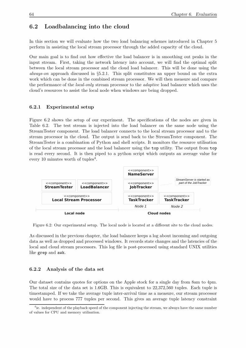
64 Chapter 6. Evaluation
6.2 Loadbalancing into the cloud
In this section we will evaluate how the two load balancing schemes introduced in Chapter 5perform in assisting the local stream processor through the added capacity of the cloud.
Our main goal is to find out how effective the load balancer is in smoothing out peaks in theinput stream. First, taking the network latency into account, we will find the optimal splitbetween the local stream processor and the cloud load balancer. This will be done using thealways-on approach discussed in §5.2.1. This split constitutes an upper bound on the extrawork which can be done in the combined stream processor. We will then measure and comparethe performance of the local-only stream processor to the adaptive load balancer which uses thecloud’s resources to assist the local node when windows are being dropped.
6.2.1 Experimental setup
Figure 6.2 shows the setup of our experiment. The specifications of the nodes are given inTable 6.2. The test stream is injected into the load balancer on the same node using theStreamTester component. The load balancer connects to the local stream processor and to thestream processor in the cloud. The output is send back to the StreamTester component. TheStreamTester is a combination of Python and shell scripts. It monitors the resource utilisationof the local stream processor and the load balancer using the top utility. The output from top
is read every second. It is then piped to a python script which outputs an average value forevery 10 minutes worth of tuples4.
Figure 6.2: Our experimental setup. The local node is located at a different site to the cloud nodes.
As discussed in the previous chapter, the load balancer keeps a log about incoming and outgoingdata as well as dropped and processed windows. It records state changes and the latencies of thelocal and cloud stream processors. This log file is post-processed using standard UNIX utilitieslike grep and awk.
6.2.2 Analysis of the data set
Our dataset contains quotes for options on the Apple stock for a single day from 8am to 4pm.The total size of the data set is 1.6GB. This is equivalent to 22,372,560 tuples. Each tuple istimestamped. If we take the average tuple inter-arrival time as a measure, our stream processorwould have to process 777 tuples per second. This gives an average tuple latency constraint
4ie. independent of the playback speed of the component injecting the stream, we always have the same numberof values for CPU and memory utilisation.
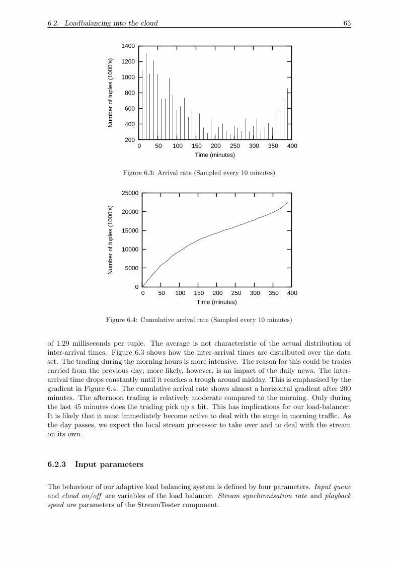
6.2. Loadbalancing into the cloud 65
200
400
600
800
1000
1200
1400
0 50 100 150 200 250 300 350 400
Num
ber
of tu
ples
(10
00’s
)
Time (minutes)
Figure 6.3: Arrival rate (Sampled every 10 minutes)
0
5000
10000
15000
20000
25000
0 50 100 150 200 250 300 350 400
Num
ber
of tu
ples
(10
00’s
)
Time (minutes)
Figure 6.4: Cumulative arrival rate (Sampled every 10 minutes)
of 1.29 milliseconds per tuple. The average is not characteristic of the actual distribution ofinter-arrival times. Figure 6.3 shows how the inter-arrival times are distributed over the dataset. The trading during the morning hours is more intensive. The reason for this could be tradescarried from the previous day; more likely, however, is an impact of the daily news. The inter-arrival time drops constantly until it reaches a trough around midday. This is emphasised by thegradient in Figure 6.4. The cumulative arrival rate shows almost a horizontal gradient after 200minutes. The afternoon trading is relatively moderate compared to the morning. Only duringthe last 45 minutes does the trading pick up a bit. This has implications for our load-balancer.It is likely that it must immediately become active to deal with the surge in morning traffic. Asthe day passes, we expect the local stream processor to take over and to deal with the streamon its own.
6.2.3 Input parameters
The behaviour of our adaptive load balancing system is defined by four parameters. Input queueand cloud on/off are variables of the load balancer. Stream synchronisation rate and playbackspeed are parameters of the StreamTester component.
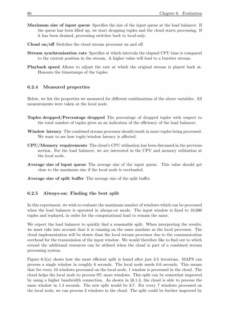
66 Chapter 6. Evaluation
Maximum size of input queue Specifies the size of the input queue at the load balancer. Ifthe queue has been filled up, we start dropping tuples and the cloud starts processing. Ifit has been drained, processing switches back to local-only.
Cloud on/off Switches the cloud stream processor on and off.
Stream synchronisation rate Specifies at which intervals the elapsed CPU time is comparedto the current position in the stream. A higher value will lead to a burstier stream.
Playback speed Allows to adjust the rate at which the original stream is played back at.Honours the timestamps of the tuples.
6.2.4 Measured properties
Below, we list the properties we measured for different combinations of the above variables. Allmeasurements were taken at the local node.
Tuples dropped/Percentage dropped The percentage of dropped tuples with respect tothe total number of tuples gives us an indication of the efficiency of the load balancer.
Window latency The combined stream processor should result in more tuples being processed.We want to see how tuple/window latency is affected.
CPU/Memory requirements The cloud’s CPU utilisation has been discussed in the previoussection. For the load balancer, we are interested in the CPU and memory utilisation atthe local node.
Average size of input queue The average size of the input queue. This value should getclose to the maximum size if the local node is overloaded.
Average size of split buffer The average size of the split buffer.
6.2.5 Always-on: Finding the best split
In this experiment, we wish to evaluate the maximum number of windows which can be processedwhen the load balancer is operated in always-on mode. The input window is fixed to 10,000tuples and replayed, in order for the computational load to remain the same.
We expect the load balancer to quickly find a reasonable split. When interpreting the results,we must take into account that it is running on the same machine as the local processor. Thecloud implementation will be slower than the local stream processor due to the communicationoverhead for the transmission of the input window. We would therefore like to find out to whichextend the additional resources can be utilised when the cloud is part of a combined streamprocessing system.
Figure 6.5(a) shows how the most efficient split is found after just 3-5 iterations. MAPS canprocess a single window in roughly 6 seconds. The local node needs 0.6 seconds. This meansthat for every 10 windows processed on the local node, 1 window is processed in the cloud. Thecloud helps the local node to process 9% more windows. This split can be somewhat improvedby using a higher bandwidth connection. As shown in §6.1.3, the cloud is able to process thesame window in 1.4 seconds. The new split would be 3-7. For every 7 windows processed onthe local node, we can process 3 windows in the cloud. The split could be further improved by
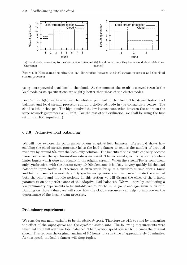
6.2. Loadbalancing into the cloud 67
0 2 4 6 8
10 12 14
1 2 3 4 5 6 7 8
Siz
e of
spl
it bu
ffer
Round
Local stream processorCloud
(a) Local node connecting to the cloud via an internet
connection
0
1
2
3
4
5
6
1 2 3
Siz
e of
spl
it bu
ffer
Round
Local stream processorCloud
(b) Local node connecting to the cloud via a LAN con-nection
Figure 6.5: Histograms depicting the load distribution between the local stream processor and the cloudstream processor
using more powerful machines in the cloud. At the moment the result is skewed towards thelocal node as its specifications are slightly better than those of the cluster nodes.
For Figure 6.5(b), we have moved the whole experiment to the cloud. The stream tester, loadbalancer and local stream processor run on a dedicated node in the college data centre. Thecloud is left unchanged. The high bandwidth, low latency connection between the nodes on thesame network guarantees a 1-1 split. For the rest of the evaluation, we shall be using the firstsetup (i.e. 10-1 input split).
6.2.6 Adaptive load balancing
We will now explore the performance of our adaptive load balancer. Figure 6.6 shows howenabling the cloud stream processor helps the load balancer to reduce the number of droppedwindows by around 8% over the local-only solution. The benefits of the cloud’s capacity becomemore clear when the synchronisation rate is increased. The increased synchronisation rate elim-inates bursts which were not present in the original stream. When the StreamTester componentonly synchronises with the stream every 10,000 elements, it is likely to very quickly fill the loadbalancer’s input buffer. Furthermore, it often waits for quite a substantial time after a burstand before it sends the next data. By synchronising more often, we can eliminate the effect ofboth the bursts and the idle periods. In this section we will discuss the effect of the 4 inputparameters on the performance of the adaptive load balancer. We will start by conducting afew preliminary experiments to fix suitable values for the input queue and synchronisation rate.Building on those values, we will show how the cloud’s resources can help to improve on theperformance of the local stream processor.
Preliminary experiments
We consider our main variable to be the playback speed. Therefore we wish to start by measuringthe effect of the input queue and the synchronisation rate. The following measurements weretaken with the full adaptive load balancer. The playback speed was set to 13 times the originalspeed. This reduces the original runtime of 6.5 hours to a run time of approximately 30 minutes.At this speed, the load balancer will drop tuples.
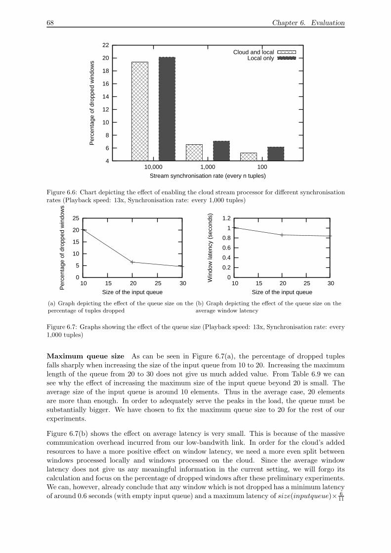
68 Chapter 6. Evaluation
4
6
8
10
12
14
16
18
20
22
10,000 1,000 100
Per
cent
age
of d
ropp
ed w
indo
ws
Stream synchronisation rate (every n tuples)
Cloud and localLocal only
Figure 6.6: Chart depicting the effect of enabling the cloud stream processor for different synchronisationrates (Playback speed: 13x, Synchronisation rate: every 1,000 tuples)
0
5
10
15
20
25
10 15 20 25 30
Per
cent
age
of d
ropp
ed w
indo
ws
Size of the input queue
(a) Graph depicting the effect of the queue size on thepercentage of tuples dropped
0
0.2
0.4
0.6
0.8
1
1.2
10 15 20 25 30Win
dow
late
ncy
(sec
onds
)
Size of the input queue
(b) Graph depicting the effect of the queue size on theaverage window latency
Figure 6.7: Graphs showing the effect of the queue size (Playback speed: 13x, Synchronisation rate: every1,000 tuples)
Maximum queue size As can be seen in Figure 6.7(a), the percentage of dropped tuplesfalls sharply when increasing the size of the input queue from 10 to 20. Increasing the maximumlength of the queue from 20 to 30 does not give us much added value. From Table 6.9 we cansee why the effect of increasing the maximum size of the input queue beyond 20 is small. Theaverage size of the input queue is around 10 elements. Thus in the average case, 20 elementsare more than enough. In order to adequately serve the peaks in the load, the queue must besubstantially bigger. We have chosen to fix the maximum queue size to 20 for the rest of ourexperiments.
Figure 6.7(b) shows the effect on average latency is very small. This is because of the massivecommunication overhead incurred from our low-bandwith link. In order for the cloud’s addedresources to have a more positive effect on window latency, we need a more even split betweenwindows processed locally and windows processed on the cloud. Since the average windowlatency does not give us any meaningful information in the current setting, we will forgo itscalculation and focus on the percentage of dropped windows after these preliminary experiments.We can, however, already conclude that any window which is not dropped has a minimum latencyof around 0.6 seconds (with empty input queue) and a maximum latency of size(inputqueue)× 6
11
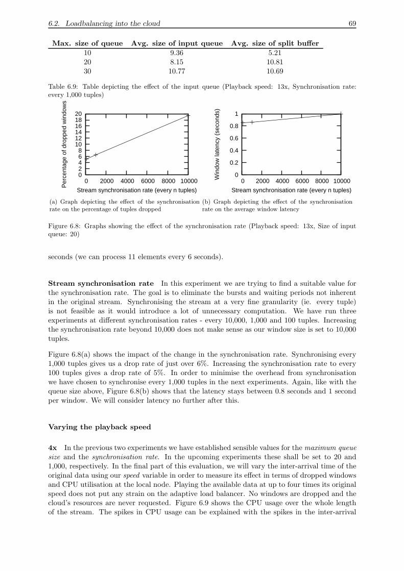
6.2. Loadbalancing into the cloud 69
Max. size of queue Avg. size of input queue Avg. size of split buffer
10 9.36 5.2120 8.15 10.8130 10.77 10.69
Table 6.9: Table depicting the effect of the input queue (Playback speed: 13x, Synchronisation rate:every 1,000 tuples)
0 2 4 6 8
10 12 14 16 18 20
0 2000 4000 6000 8000 10000
Per
cent
age
of d
ropp
ed w
indo
ws
Stream synchronisation rate (every n tuples)
(a) Graph depicting the effect of the synchronisationrate on the percentage of tuples dropped
0
0.2
0.4
0.6
0.8
1
0 2000 4000 6000 8000 10000Win
dow
late
ncy
(sec
onds
)
Stream synchronisation rate (every n tuples)
(b) Graph depicting the effect of the synchronisationrate on the average window latency
Figure 6.8: Graphs showing the effect of the synchronisation rate (Playback speed: 13x, Size of inputqueue: 20)
seconds (we can process 11 elements every 6 seconds).
Stream synchronisation rate In this experiment we are trying to find a suitable value forthe synchronisation rate. The goal is to eliminate the bursts and waiting periods not inherentin the original stream. Synchronising the stream at a very fine granularity (ie. every tuple)is not feasible as it would introduce a lot of unnecessary computation. We have run threeexperiments at different synchronisation rates - every 10,000, 1,000 and 100 tuples. Increasingthe synchronisation rate beyond 10,000 does not make sense as our window size is set to 10,000tuples.
Figure 6.8(a) shows the impact of the change in the synchronisation rate. Synchronising every1,000 tuples gives us a drop rate of just over 6%. Increasing the synchronisation rate to every100 tuples gives a drop rate of 5%. In order to minimise the overhead from synchronisationwe have chosen to synchronise every 1,000 tuples in the next experiments. Again, like with thequeue size above, Figure 6.8(b) shows that the latency stays between 0.8 seconds and 1 secondper window. We will consider latency no further after this.
Varying the playback speed
4x In the previous two experiments we have established sensible values for the maximum queuesize and the synchronisation rate. In the upcoming experiments these shall be set to 20 and1,000, respectively. In the final part of this evaluation, we will vary the inter-arrival time of theoriginal data using our speed variable in order to measure its effect in terms of dropped windowsand CPU utilisation at the local node. Playing the available data at up to four times its originalspeed does not put any strain on the adaptive load balancer. No windows are dropped and thecloud’s resources are never requested. Figure 6.9 shows the CPU usage over the whole lengthof the stream. The spikes in CPU usage can be explained with the spikes in the inter-arrival
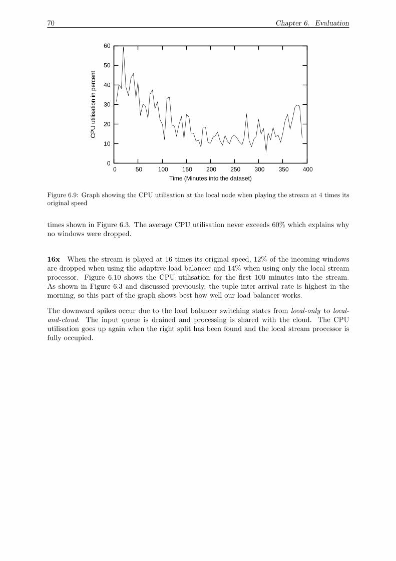
70 Chapter 6. Evaluation
0
10
20
30
40
50
60
0 50 100 150 200 250 300 350 400
CP
U u
tilis
atio
n in
per
cent
Time (Minutes into the dataset)
Figure 6.9: Graph showing the CPU utilisation at the local node when playing the stream at 4 times itsoriginal speed
times shown in Figure 6.3. The average CPU utilisation never exceeds 60% which explains whyno windows were dropped.
16x When the stream is played at 16 times its original speed, 12% of the incoming windowsare dropped when using the adaptive load balancer and 14% when using only the local streamprocessor. Figure 6.10 shows the CPU utilisation for the first 100 minutes into the stream.As shown in Figure 6.3 and discussed previously, the tuple inter-arrival rate is highest in themorning, so this part of the graph shows best how well our load balancer works.
The downward spikes occur due to the load balancer switching states from local-only to local-and-cloud. The input queue is drained and processing is shared with the cloud. The CPUutilisation goes up again when the right split has been found and the local stream processor isfully occupied.
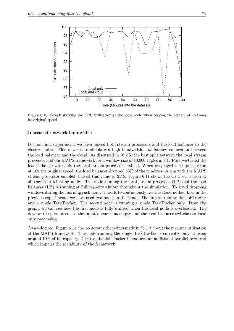
6.2. Loadbalancing into the cloud 71
84
86
88
90
92
94
96
98
100
10 20 30 40 50 60 70 80 90 100
CP
U u
tilis
atio
n in
per
cent
Time (Minutes into the dataset)
Local onlyLocal and cloud
Figure 6.10: Graph showing the CPU utilisation at the local node when playing the stream at 16 timesits original speed
Increased network bandwidth
For our final experiment, we have moved both stream processors and the load balancer to thecluster nodes. This move is to simulate a high bandwidth, low latency connection betweenthe load balancer and the cloud. As discussed in §6.2.5, the best split between the local streamprocessor and our MAPS framework for a window size of 10,000 tuples is 1-1. First we tested theload balancer with only the local stream processor enabled. When we played the input streamat 16x the original speed, the load balancer dropped 53% of the windows. A run with the MAPSstream processor enabled, halved this value to 25%. Figure 6.11 shows the CPU utilisation atall three participating nodes. The node running the local stream processor (LP) and the loadbalancer (LB) is running at full capacity almost throughout the simulation. To avoid droppingwindows during the morning rush hour, it needs to continuously use the cloud nodes. Like in theprevious experiments, we have used two nodes in the cloud. The first is running the JobTrackerand a single TaskTracker. The second node is running a single TaskTracker only. From thegraph, we can see how the first node is fully utilised when the local node is overloaded. Thedownward spikes occur as the input queue runs empty and the load balancer switches to localonly processing.
As a side note, Figure 6.11 also re-iterates the points made in §6.1.3 about the resource utilisationof the MAPS framework. The node running the single TaskTracker is currently only utilisingaround 10% of its capacity. Clearly, the JobTracker introduces an additional parallel overheadwhich impairs the scalability of the framework.
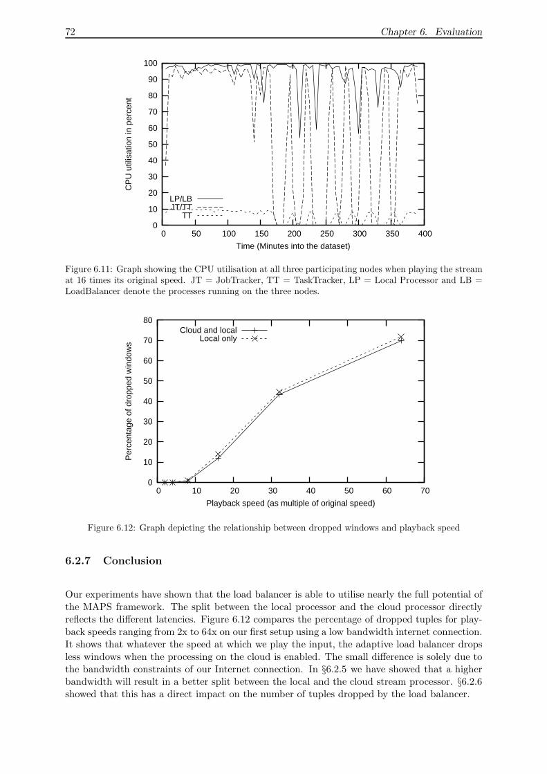
72 Chapter 6. Evaluation
0
10
20
30
40
50
60
70
80
90
100
0 50 100 150 200 250 300 350 400
CP
U u
tilis
atio
n in
per
cent
Time (Minutes into the dataset)
LP/LBJT/TT
TT
Figure 6.11: Graph showing the CPU utilisation at all three participating nodes when playing the streamat 16 times its original speed. JT = JobTracker, TT = TaskTracker, LP = Local Processor and LB =LoadBalancer denote the processes running on the three nodes.
0
10
20
30
40
50
60
70
80
0 10 20 30 40 50 60 70
Per
cent
age
of d
ropp
ed w
indo
ws
Playback speed (as multiple of original speed)
Cloud and localLocal only
Figure 6.12: Graph depicting the relationship between dropped windows and playback speed
6.2.7 Conclusion
Our experiments have shown that the load balancer is able to utilise nearly the full potential ofthe MAPS framework. The split between the local processor and the cloud processor directlyreflects the different latencies. Figure 6.12 compares the percentage of dropped tuples for play-back speeds ranging from 2x to 64x on our first setup using a low bandwidth internet connection.It shows that whatever the speed at which we play the input, the adaptive load balancer dropsless windows when the processing on the cloud is enabled. The small difference is solely due tothe bandwidth constraints of our Internet connection. In §6.2.5 we have showed that a higherbandwidth will result in a better split between the local and the cloud stream processor. §6.2.6showed that this has a direct impact on the number of tuples dropped by the load balancer.
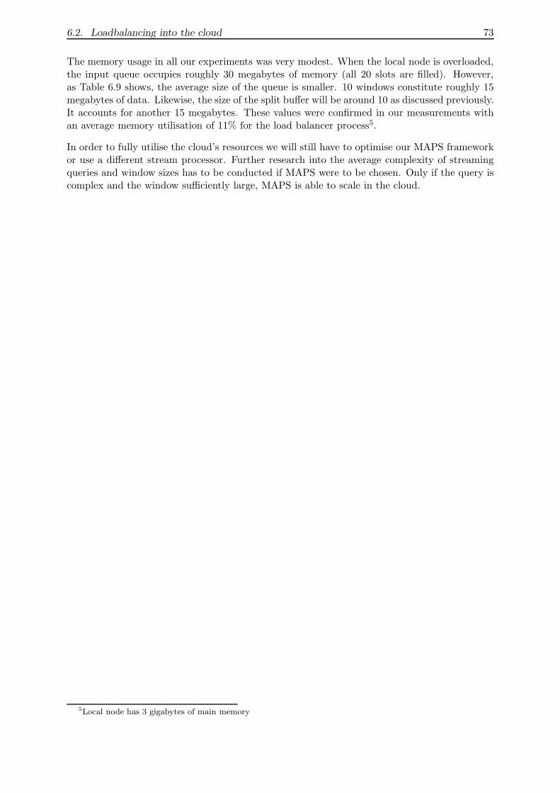
6.2. Loadbalancing into the cloud 73
The memory usage in all our experiments was very modest. When the local node is overloaded,the input queue occupies roughly 30 megabytes of memory (all 20 slots are filled). However,as Table 6.9 shows, the average size of the queue is smaller. 10 windows constitute roughly 15megabytes of data. Likewise, the size of the split buffer will be around 10 as discussed previously.It accounts for another 15 megabytes. These values were confirmed in our measurements withan average memory utilisation of 11% for the load balancer process5.
In order to fully utilise the cloud’s resources we will still have to optimise our MAPS frameworkor use a different stream processor. Further research into the average complexity of streamingqueries and window sizes has to be conducted if MAPS were to be chosen. Only if the query iscomplex and the window sufficiently large, MAPS is able to scale in the cloud.
5Local node has 3 gigabytes of main memory

74 Chapter 6. Evaluation
Chapter 7
Conclusion
In this report have used a cloud-based stream processor to investigate load balancing strategiesto efficiently handle bursts in the input stream. We claim that utilising the cloud to handle peakload situations can significantly reduce the costs of stream processing.
Previous stream processing systems have already discussed the parallelisation of queries [13] [29].Mortar uses an overlay network and distributes the operators over a tree [29]. This helps todeal with failures but does not make a distinction between normal and peak load. Cayuga’spublish subscribe system allows queries to be pipelined [13]. Pipelining is dependent on thequery and not very scalable. The row/column scaling approach also mentioned in Logothetisand Yocum [13] uses available resources in a round-robin fashion. This scales very well when thequeries are stateless. However, when queries are stateful, the input stream has to be split androuted to the correct node. In this report we have chosen to adopt the MapReduce programmingmodel for our cloud stream processor to investigate an alternative approach which scales thequery over a number of machines based on the size of the input.
7.1 Project review
In the first part of this report we have shown how a MapReduce stream processing system canbe implemented on a homogeneous cluster. In the second part we have shown how a local streamprocessor can utilise the cloud’s resources to deal with bursts in the input stream.
7.1.1 Contributions
Streaming extension for the Hadoop framework In §3 we have discussed the implemen-tation of the extensions necessary to receive input from a stream in the Hadoop framework.We have measured the performance of this solution and explained why its overheads currentlyprohibit efficient stream processing.
MAPS: A Lightweight MapReduce framework Building on the experience from extend-ing the Hadoop framework, we have designed and implemented MAPS, a lightweight MapReduceframework written in Python (§4). We have showed how the elimination of the distributed filesystem significantly reduces the parallel overhead and leads to a more stable run time. In ourevaluation of the system we have showed how the scalability of a query is closely linked to the
75
76 Chapter 7. Conclusion
complexity of its map and reduce functions as well as the size of the input window. These obser-vations confirm previous work on distributed stream processing as operator placement (Mortar)and pipelining (Cayuga) both depend on the query being split up for parallelisation.
Loadbalancing strategies In §5 we have discussed the design and implementation of tworelated load balancing solutions which make use of cloud resources to relieve a local streamprocessor.
By utilising our MAPS prototype on a cluster infrastructure, we have showed how our always-on loadbalancer can increase the total number of windows processed by combining the cloudand local stream processors. In the adaptive setting, our load balancer is able to utilise cloudresouces on-demand to reduce the number of windows dropped.
In §6.2.5 we have showed how the efficiency of the MAPS cloud processor varies with the band-width of the connection between the local node and the cloud. We have showed that thebandwidth between the local node and the cloud is a more decisive factor for the number ofwindows dropped than the latency of the connection.
7.2 Future work
7.2.1 Improving the efficiency of the MapReduce framework
In Chapter 4 we have motivated our choice for Python as implementation language. As ourMapReduce framework was merely a prototype, this choice was acceptable. In order to fullyutilise the potential of the cloud’s resources, we would develop a more efficient version in Java orC. Subject to the technology made available by the chosen cloud provider, it would be sensibleto use an efficient message-passing framework like MPI in order to minimise the communicationcost. This is especially important as computation time on the cloud has monetary implications.
7.2.2 Pipelined MapReduce jobs
Cayuga’s pipelining approach can be easily applied to our MapReduce framework by allowing formultiple, chained MapReduce jobs. Chaining multiple MapReduce jobs does not only potentiallyhelp with scaling the query; it also allows us to write more expressive queries. However, carefulattention must be paid to the complexity of the individual queries in order to make sure it isnot dropping below a threshold where communication becomes a bottleneck.
7.2.3 MAPS scaling
The best number of TaskTrackers to use for a certain window size should be found automatically.Currently, the MAPS framework uses as many TaskTrackers as are registered to the name server.A future version of this framework must take the cost of computing data on the cloud as well asthe scalability of the query into account and decide an optimum value for the number of nodesparticipating in the MapReduce process. MAPS supports threaded reduce tasks. Due to timeconstraints, we have left their evaluation for future work. The MapReduce framework shouldideally not only scale over nodes but utilise all available processing power on each one of themin an effort to reduce inter-node communication.
7.2. Future work 77
7.2.4 Adapting Cayuga to scale on a cloud infrastructure
The evaluation has showed that MapReduce does not efficiently scale when small windows andcomputationally less intensive queries are used. In order to make the best use of the cloud’scapacity, we suggest to adapt the distributed Cayuga implementation for a cloud infrastructure.Row/column scaling can be used to balance less complex queries. For more complex queriesand larger window sizes it may be considered to compile the CQL queries to MapReduce jobs.Fusing Cayuga and MapReduce technology could possibly help to overcome the performancebottlenecks arising from handling stateful queries.
7.2.5 Eliminating communication bottlenecks
Splitting the input stream Concerning the load balancer, further research into splitting thestream closer to the source or subscribing both the local node and the cloud to the same inputstream should be conducted. If we can find a way to forgo the copying of data between the localnode and the cloud, we can significantly reduce the latency. An interesting aspect of this willbe the control flow between the local node and the cloud to coordinate which windows shouldbe processed on the two stream processors.
Query-aware load balancing The communication between the local node and the cloudcould be reduced by a query-aware loadbalancer which only send the elements of the tuples tothe cloud which are necessary for the computation of the MapReduce query. Essentially, theload-balancer operates as a first instance map function to prepare the data for the cloud. Inour case the data is reduced from 20 to 3 words per tuple after the initial map function. If thishad been done by the load balancer, we could have significantly reduced the overhead from thecommunication.
Window compression In addition, we could have further reduced the communication over-head by compressing the input window. An input window may contain duplicates. More impor-tantly, however, we might be able to take advantage of the fact that most of the data is numericand rather short. Sending a 2 digit number over the network using 2 chars is not efficient.
7.2.6 Parallel programming with language support - F#
Our MAPS implementation has showed that it is possible to write a distributed MapReduceframework in a functional language. Microsoft’s F# programming language has parallel con-structs already built in. Further work could look directly at distributing functional programs inMapReduce style over a set of nodes. Tying in with the previous point, this could mean thatthe low level communication is handled by fast native code while at the same time retaining thebenefits of an expressive functional programming language for designing the query.
7.2.7 Cost-benefit analysis
It is very important to conduct a proper cost-benefit analysis before any computation is movedto the cloud. As mentioned in the introduction, it makes sense to use a cloud provider for streamprocessing tasks when the servers are only needed a maximum of 6 hours a day and are not usedon weekends. In addition, when trying to achieve low-latency responses to market conditions,

78 Chapter 7. Conclusion
the location of the cloud nodes becomes important. EC2 nodes in North America will not besuited to place trades at the HKEx in Hong Kong. However, if nodes in close proximity to thestock exchanges are available, the cloud based solution becomes very attractive. While buildinga new data centre in the vincinity of the market is infeasible, a cloud-based solution can beimplemented at a very small cost. Further research into the latency properties of existing cloudsolutions has to be conducted to quantify these benefits.
Bibliography
[1] Hadoop FAQ. URL http://wiki.apache.org/hadoop/FAQ. Accessed on 27/01/10.
[2] Hadoop MapReduce tutorial. URL http://hadoop.apache.org/common/docs/current/
mapred_tutorial.html. Accessed on 27/01/10.
[3] ZooKeeper. URL http://hadoop.apache.org/zookeeper. Accessed on 27/01/10.
[4] More chip cores can mean slower supercomputing, Sandia simulation shows, January 12,2009. URL http://www.physorg.com/news151158992.html. Accessed on 01/06/10.
[5] SalesForce (Cloud Provider). URL http://www.salesforce.com. Accessed on 05/06/10.
[6] Joyent (Cloud Provider). URL http://www.joyent.com/. Accessed on 05/06/10.
[7] RightScale Cloud Management Platform. URL http://www.rightscale.com. Accessedon 05/06/10.
[8] STAN - an eclipse based structural analysis tool. URL http://www.stan4j.com. Accessedon 15/03/10.
[9] A. Arasu, B. Babcock, S. Babu, J. Cieslewicz, M. Datar, K. Ito, R Motwani, U. Srivastava,and J. Widom. Stream: The stanford data stream management system. Technical Report2004-20, Stanford InfoLab, 2004. URL http://ilpubs.stanford.edu:8090/641/.
[10] Matt Asay. Q&A: Visa dips a toe into the Hadoop pool. Cnet.com - The Open Road,September 17, 2009. URL http://news.cnet.com/openroad/?keyword=Hadoop.
[11] Jeff Barr. Amazon EC2 Beta, August 2006. URL http://aws.typepad.com/aws/2006/
08/amazon_ec2_beta.html. Accessed on 13/01/10.
[12] Chris Bemis. Put-Call Parity, 2006. URL http://www.math.umn.edu/finmath/seminar/
bemisslidesB.pdf. Accessed on 20/12/09.
[13] Lars Brenna, Johannes Gehrke, Mingsheng Hong, and Dag Johansen. Distributed eventstream processing with non-deterministic finite automata. In DEBS ’09: Proceedings ofthe Third ACM International Conference on Distributed Event-Based Systems, pages 1–12,New York, NY, USA, 2009. ACM. ISBN 978-1-60558-665-6. doi: http://doi.acm.org/10.1145/1619258.1619263.
[14] H. Bryhni, E. Klovning, and O. Kure. A comparison of load balancing techniques forscalable web servers. IEEE Network, 14(4):58–64, 2000.
[15] Valeria Cardellini, Emiliano Casalicchio, Michele Colajanni, and Philip S. Yu. The stateof the art in locally distributed web-server systems. ACM Comput. Surv., 34(2):263–311,2002. ISSN 0360-0300. doi: http://doi.acm.org/10.1145/508352.508355.
79
80 BIBLIOGRAPHY
[16] Constantin Christmann, Juergen Falkner, Dietmar Kopperger, and Anette Weisbecker.Schein oder Sein: Kosten und Nutzen von Cloud Computing. iX Special 2/2010 - Cloud,Grid, Virtualisierung, pages 6–9, February 2010.
[17] Ariel Cohen, Sampath Rangarajan, and Hamilton Slye. On the performance of tcp splicingfor url-aware redirection. In USITS’99: Proceedings of the 2nd conference on USENIXSymposium on Internet Technologies and Systems, pages 11–11, Berkeley, CA, USA, 1999.USENIX Association.
[18] T. Condie et al. MapReduceOnline. Technical Report UCB/EECS-2009-136, UCB, 2009.
[19] Jeffrey Dean and Sanjay Ghemawat. Mapreduce: simplified data processing on large clus-ters. Commun. ACM, 51(1):107–113, 2008. ISSN 0001-0782. doi: http://doi.acm.org/10.1145/1327452.1327492.
[20] Alan Demers, Johannes Gehrke, Mingsheng Hong, Mirek Riedewald, and Walker White.Towards expressive publish/subscribe systems. In Advances in Database Technology - EDBT2006, volume 3896 of Lecture Notes in Computer Science, pages 627–644. Springer Berlin/ Heidelberg, 2006. ISBN 978-3-540-32960-2. doi: 10.1007/11687238 38. URL http:
//www.springerlink.com/content/y684305339173080/.
[21] Mara Der Hovanesian. Cracking The Street’s New Math. BusinessWeek, April 18, 2005.URL http://www.businessweek.com/magazine/content/05_16/b3929113_mz020.htm.
[22] David DeWitt and Michael Stonebraker. MapReduce: A major step back-wards. URL http://databasecolumn.vertica.com/database-innovation/
mapreduce-a-major-step-backwards/. Accessed on 14/12/09.
[23] Domenico Ferrari and Songnian Zhou. An empirical investigation of load indices for loadbalancing applications. In Performance ’87: Proceedings of the 12th IFIP WG 7.3 Inter-national Symposium on Computer Performance Modelling, Measurement and Evaluation,pages 515–528, Amsterdam, The Netherlands, The Netherlands, 1988. North-Holland Pub-lishing Co. ISBN 0-444-70347-0.
[24] Ian Foster, Carl Kesselman, and Steven Tuecke. The anatomy of the grid: Enabling scalablevirtual organizations. Int. J. High Perform. Comput. Appl., 15(3):200–222, 2001. ISSN1094-3420. doi: http://dx.doi.org/10.1177/109434200101500302.
[25] Charles Hayden. Announcing the Map/Reduce Toolkit. New York Times - Open Blog, May11, 2009. URL http://open.blogs.nytimes.com/tag/hadoop.
[26] Vipin Kumar. Introduction to Parallel Computing. Addison-Wesley Longman PublishingCo., Inc., Boston, MA, USA, 2002. ISBN 0201648652.
[27] Marcel Kunze and Christian Baun. Wolkige Zeiten, Cloud Computing: Hype vor derKonsolidierung. iX Special 1/2010 - Programmieren heute, pages 111–116, January 2010.
[28] S. Loebman, D. Nunley, Y.C. Kwon, B. Howe, M. Balazinska, and J.P. Gardner. AnalyzingMassive Astrophysical Datasets: Can Pig/Hadoop or a Relational DBMS Help?
[29] Dionysios Logothetis and Kenneth Yocum. Wide-scale data stream management. InATC’08: USENIX 2008 Annual Technical Conference on Annual Technical Conference,pages 405–418, Berkeley, CA, USA, 2008. USENIX Association.
[30] Sun Microsystems. RPC: Remote Procedure Call Protocol specification: Version 2. RFC1057 (Informational), June 1988. URL http://www.ietf.org/rfc/rfc1057.txt.
BIBLIOGRAPHY 81
[31] Nasdaq. Market Share Statistics. URL http://www.nasdaqtrader.com/trader.aspx?id=
marketshare. Accessed on 10/01/10.
[32] Vivek S. Pai, Mohit Aron, Gaurov Banga, Michael Svendsen, Peter Druschel, WillyZwaenepoel, and Erich Nahum. Locality-aware request distribution in cluster-based net-work servers. SIGPLAN Not., 33(11):205–216, 1998. ISSN 0362-1340. doi: http://doi.acm.org/10.1145/291006.291048.
[33] Aaron Pan. Algo-trading is a strategic focus, says Nomura. Asiamoney, 21, April 2010.
[34] Rob Pike, Sean Dorward, Robert Griesemer, and Sean Quinlan. Interpreting the data:Parallel analysis with sawzall. Sci. Program., 13(4):277–298, 2005. ISSN 1058-9244.
[35] Justin Smith. Facebook Using Hadoop for Large Scale Internal Analytics. In-side Facebook, June 6, 2008. URL http://www.insidefacebook.com/2008/06/06/
facebook-using-hadoop-for-large-scale-internal-analytics.
[36] Michael Stonebraker, Daniel Abadi, David J. DeWitt, Sam Madden, Erik Paulson, AndrewPavlo, and Alexander Rasin. Mapreduce and parallel dbmss: friends or foes? Com-mun. ACM, 53(1):64–71, 2010. ISSN 0001-0782. doi: http://doi.acm.org/10.1145/1629175.1629197.
[37] Sun Microsystems. Remote Method Invocation (RMI). URL http://java.sun.com/
javase/technologies/core/basic/rmi/index.jsp. Accessed on 17/05/10.
[38] Andrew S. Tanenbaum. Computer networks: 2nd edition. Prentice-Hall, Inc., Upper SaddleRiver, NJ, USA, 1988. ISBN 0-13-162959-X.
[39] Andrew S. Tanenbaum and Maarten van Steen. Distributed Systems: Principles andParadigms (2nd Edition). Prentice-Hall, Inc., Upper Saddle River, NJ, USA, 2006. ISBN0132392275.
[40] Heather Timmons. A London Hedge Fund That Opts for Engineers, Not M.B.A.’s. NewYork Times, August 18, 2006. URL http://www.nytimes.com/2006/08/18/business/
worldbusiness/18man.html?_r=1&ex=1313553600.