strength model of concrete using heat and microstructure ... · i strength model of concrete using...
TRANSCRIPT

i
Strength Model of Concrete Using Heat and Microstructure Developments
HAN Virak
A dissertation submitted to Kochi University of Technology
In partial fulfillment of the requirements for the degree of
Doctor of Engineering
Graduate School of Engineering Kochi University of Technology
Kochi, Japan
August 2006

ii
Strength Model of Concrete Using Heat and
Microstructure Developments
HAN Virak
B.Eng (Institute of Technology of Cambodia, Cambodia) 1998 M. Eng (Universite Libre de Bruxelles, Belgium) 2001
A dissertation submitted to Kochi University of Technology
In partial fulfillment of the requirements for the degree of
Doctor of Engineering
Special Course for International Students
Department of Engineering Graduate School of Engineering
Infrastructure System Engineering Kochi University of Technology
Kochi, Japan
Examination Committee: Professor SHIMA Hiroshi (advisor) Professor OKAMURA Hajime Professor KUSAYANAGI Shunji Professor FUJISAWA Nobumitsu Assoc. Professor OUCHI Masahiro
August 2006

iii
ACKNOWLEDGEMENTS
First of all, I would like to write down some of my gratitude owed to all persons who have offered directly or indirectly their useful helps for the completion of this thesis. The particular thanks are pronounced to my advisor, Prof. Hiroshi SHIMA for his advice in steering my studies of concerned theories as well as experimental works and for his opinions in discussion since the beginning of the research. Without his considerable contributions, this thesis can not be successfully published.
Thanks are not forgotten to Prof. Hajime OKAMURA for his important advice in establishing a strength model which is the target of the research and to Prof. Masahiro OUCHI for his useful suggestions for the research.
In my study, I have learned from the seminars which were held every week in a manner so friendly and educational that a diversity of ideas can be exchanged between researchers. Thanks are frankly expressed to all the concrete laboratory members.
It is really my great delight to have the jury board composed of Prof. Hiroshi SHIMA, Prof. Masahiro OUCHI, Prof. Hajime OKAMURA, Prof. Nobumitsu FUJISAWA and Prof. Shunji KUSAYANAGI. Their constructive suggestions and kindness made me not only write the names in this piece of paper but also engrave deeply in my heart forever.
The analysis in the research is concerned with strength, porosity and heat. I acknowledge the kindness of Prof. Toshiharu Kishi in providing the code written in Fortran with which the heat calculation was operated. Sincere thanks to Dr. Supakit Swatekititham and Dr. Ming-Hung Hsieh are kept in heart for their kind explanations in guiding me during when I was very new to the concrete laboratories of KUT. Thanks are also owed to Miss Sachie Kokubo for her helpful contributions during my study. The experimental works were conducted with help of my classmate Mr. VONG Seng, particularly when the work was hard and could not be conducted alone. His contribution was gratefully considered as an indispensable intervention.
I acknowledge the SSP scholarship of KUT with which I could live and study in Japan for 3 years. In addition, IRC (international relation center) members have undertaken very kind helps in solving living problems as well as in facilitating many administrative procedures. Without their effective interventions, life was not happy. They deserve my great gratitude.

iv
ABSTRACT
In concrete engineering, strength of concrete is one of the important indexes that concrete engineers should know. The strength has been found basing on some basic formula called the strength model which is usually used for the purpose of mix adjustment in the mix design method. In general, a number of trial mixes are always needed before obtaining a target mix proportion. According to the properties required, it takes at least one month or more in order to achieve enough satisfaction. Many researchers have made their efforts in creating strength models able to give more precise prediction with a reduced amount of trial mixes. Many models were proposed basing on some practical parameters which may not the determinant ones and the applications were limited. The main purpose of this research is to establish a strength model capable of estimating the strength of cement, mortar and concrete at any age without conducting any trial mixes and basing only on the provided data including composing powders, mix proportions, curing conditions and ages. The mechanism of strength development is very well concerned with an increase of hydration products accompanying the pore reduction. Recently the theories of microstructure development and multi-component hydration development were successfully proposed and were widely used in estimating concrete durability. With these theories, the porosities of any kinds and heat of hydration of any component powders as well as minerals can be accurately calculated only if the chemical and physical properties of materials used are known. So the attempt to create the strength model without trial mixes becomes a good challenge. The microstructure and heat models can give good results only when the proportion of good mixes is provided, too bad mixes are not recommended. The first work is then to find the simulated mixes that are not so much segregated or bleeded that the strength is affected. One remarkable property of cement that is contrary to the ideal property of the multi-component heal model is that when mixing the flocculation of particles occur unavoidably due to the absorption without dispersion however in the model, powder particles were considered as well dispersed in uniform spaces and hydration was uniform at each particles. The problem of particle flocculation can be solved by introducing dispersing agents known as super-plasticizers (SP) which are widely used in concrete production. Daimon et al. clarified that SP possesses principally 3 actions in dispersing cement particles. These actions are repulsive force due to the increase of zeta-energy, liquid-solid affinity and steric hindrance. The higher the dispersion, the more hydration products are precipitated the strength is then increased so the suitable mix which has the ideal dispersion is the mix of high strength among different mixes of the same mix proportion with variation of the dispersing SP dosages. Beside the dispersion

v
effect, other effects on strength played by aggregate content and mixing times were also studied. The authors made 3 main series of mortar mixes after which the SP dosage, sand content and mixing time could be decided. When the mixes were defined, more mixes were produced for the purpose of modeling. The modeling is conducted by formulating strength tested on cylindrical specimens as function of hydration heat of each compounds and effective porosity of mixes which are calculated. Different types of Portland cements were used and a wide range of w/c ratios with the wet and sealed curing conditions were considered. The results have shown that strength holds linear relations with the heat of each compound coupled with porosity. The combination of heat and pore as a single parameter is hereafter called as heat-pore component. It becomes clear that the strength can be modeled with a sum of each heat-pore component multiplied by strength contribution of each compound. Basing on the authors' experimental data, the strength contribution of each compound is determined. The strength model is created for wide application of Portland cements. The models for blended cements were also studied by introducing the powder contribution coefficients. The model applicable for blended cement is then proposed. The model was established with mixes free of sand content effect so when it is used for concrete, aggregate effect should be considered as another parameter.

vi
TABLE OF CONTENTS
Names Page numbers
ACKNOWLEDGEMENTS .................................................................................................iii ABSTRACT ......................................................................................................................... iv TABLE OF CONTENTS...................................................................................................... vi LIST OF TABLES..............................................................................................................viii LIST OF FIGURES.............................................................................................................. ix CHAPTER I: INTRODUCTIONS................................................................................... 1 I. Introductions................................................................................................................... 1 I.1. Research requirements ................................................................................................ 1 I.2. Strength model history ................................................................................................ 2 I.3. Research programs...................................................................................................... 6 CHAPTER II: LITERATURE ......................................................................................... 8 II. Literature Reviews ...................................................................................................... 8 II.1. Microstructure model .................................................................................................. 8 II.2. Multi-component heat model .................................................................................... 11 II.3. Porosity measurement and the disadvantages........................................................... 19 II.4. Integration of microstructure and multi-component heat model .............................. 21 CHAPTER III: METHODOLOGY .................................................................................. 23 III. Methodology ............................................................................................................. 23 III.1. Materials ................................................................................................................ 23 III.1.A. Admixtures......................................................................................................... 23 III.1.B. Cements.............................................................................................................. 24 III.1.C. Powders.............................................................................................................. 25 III.1.D. Sands .................................................................................................................. 26 III.2. Mixer and mixing .................................................................................................. 28 III.3. Curing conditions .................................................................................................. 29 III.4. Testing methods..................................................................................................... 30 III.4.A. Sampling, specimen size and age....................................................................... 30 III.4.B. Surfacing ............................................................................................................ 30 III.4.C. Compressive strength test .................................................................................. 31 CHAPTER IV: MIX PROPORTIONING ........................................................................ 33 IV. Mix proportioning ..................................................................................................... 33 IV.1. Fundamental proportioning ................................................................................... 33 IV.2. Mortar in concrete ................................................................................................. 35 CHAPTER V: DATA DISCUSSION .............................................................................. 38

vii
V. Data discussion............................................................................................................. 38 V.1. Strength and sand content ......................................................................................... 38 V.2. Strength and dosage of SP......................................................................................... 41 V.3. Strength and mixing times ........................................................................................ 44 V.4. Strength behavior when limestone powder is used................................................... 47 CHAPTER VI: MODELING............................................................................................ 52 VI. Modeling ................................................................................................................... 52 VI.1. Ideal mixes and their properties............................................................................. 52 VI.2. Strength with its determinant factors..................................................................... 54 VI.2.A. Strength mechanism........................................................................................... 54 VI.2.B. Strength with heat and porosity ......................................................................... 55 VI.3. Proposed model ..................................................................................................... 57
VI.3.A. Strength function with P
H i ............................................................................... 57
VI.3.B. Strength function with iHPI
PPI .− .................................................................... 60
VI.3.C. Contribution of compounds with age................................................................. 62 VI.4. Model with slag and fly ash replacement .............................................................. 64 VI.5. Model for mixes with LS....................................................................................... 64 VI.6. Two-compound modeling...................................................................................... 66 VI.6.A. Two-compound model for Portland cements ..................................................... 67 VI.6.B. Two-compound model for Powder replacement ................................................ 68 VI.7. Prediction for other sources of data....................................................................... 68 VI.8. Applicability of model........................................................................................... 70 CHAPTER VII: CONCLUSIONS.................................................................................... 71 VII. Conclusions............................................................................................................... 71 VII.1. General conclusions............................................................................................... 71 VII.2. Model improvement .............................................................................................. 72 CHAPTER VIII: APPENDIXES ...................................................................................... 74 VIII. Appendixes ............................................................................................................ 74 VIII.1. Preliminary mix data.......................................................................................... 74 VIII.2. Strength and porosity: Hi/P................................................................................ 81 VIII.3. Strength and porosity: Hi*(PI-EP)/PI ................................................................ 88 VIII.4. Data of Sumitomo Osaka and UBE-Mitsubishi cements................................... 96 VIII.5. Pore effects....................................................................................................... 100 REFERENCES .................................................................................................................. 104

viii
LIST OF TABLES Table II.2-1: Delaying effect corresponding to each type of admixtures ............................ 18 Table III.1.B-1: Cement compositions ................................................................................ 25 Table III.1.C-1: Powder properties...................................................................................... 26 Table III.1.D-1: Sand properties.......................................................................................... 26 Table V.2-1: SP maximum effect for different w/c.............................................................. 43 Table V.4-1: SP dosage with and without LS ...................................................................... 48 Table VI.1-1: Strength of ideal mixes with LH ................................................................... 52 Table VI.1-2: Strength of ideal mixes with OPC................................................................. 52 Table VI.1-3: Strength of ideal mixes with HES................................................................. 53 Table VI.3.C-1 Contributive coefficients of compounds as a function of age ................. 62 Table VI.7-1: Main differences of other sources of data ..................................................... 69 Table VI.8-1: Portland cements and CACs ......................................................................... 70 Table VIII.1-1: Mix properties w/c=0.3-(3 minute mixing times), sealed condition .......... 74 Table VIII.1-2: Mix properties w/c=0.6-(3 minute mixing times), sealed condition .......... 75 Table VIII.1-3: Mix properties w/c=0.3, seal condition...................................................... 76 Table VIII.1-4: Mix properties w/c=0.6, seal condition...................................................... 76 Table VIII.1-5: Mix proportion of mortars using low heat, OPC and high early
strength cements ...................................................................................... 77 Table VIII.1-6: Mix proportions with powders ................................................................... 78 Table VIII.1-7: Test results of mixes with limestone replacement...................................... 79 Table VIII.1-8: Dosage of SP for mixes with fly ash replacement...................................... 80 Table VIII.1-9 Strength of mortars with fly ash replacement.......................................... 80 Table VIII.1-10: SP dosage for slag replacement mixes ..................................................... 80 Table VIII.1-11: Strength for mixes with slag replacement ................................................ 80 Table VIII.2-1: Hi/EP for LH cement mortar ...................................................................... 81 Table VIII.2-2: Hi/EP for HES cement mortar.................................................................... 82 Table VIII.2-3: Hi/EP for OPC mortar ................................................................................ 83 Table VIII.3-1: Hi*(Vw-EP)/Vw for LH cement mortar .................................................... 88 Table VIII.3-2: Hi*(Vw-EP)/Vw for OPC and HES mortars.............................................. 89 Table VIII.3-3: Hi*(Vw-EP)/Vw for Limestone and slag mortars...................................... 90 Table VIII.3-4: Hi*(Vw-EP)/Vw for flyash mortar ............................................................ 91 Table VIII.4-1 Compositions of cements provided by Sumitomo Osaka cement ........... 96 Table VIII.4-2 Strength of standard mortars by Sumitomo Osaka cement ..................... 96 Table VIII.4-3 Cement composition of UBE-Mitsubishi corporation............................. 96 Table VIII.4-4 Strength of standard mortars by UBE-Mitsubishi corporation................ 97

ix
Table VIII.4-5 Mix proportions of normal concrete by UBE-MItsubishi ....................... 97 Table VIII.4-6 Strength of normal concrete provided by UBE-Mitsubishi..................... 98 Table VIII.4-7 Mix proportions of high strength concrete by UBE-Mitsubishi.............. 99 Table VIII.4-8 Strength of high strength concrete Provided by UBE-Mitsubishi ........... 99 Table VIII.5-1: Data for fictive porosity calculation for LH............................................. 101 Table VIII.5-2: Data for fictive porosity calculation for OPC .......................................... 102 Table VIII.5-3: Data for fictive porosity calculation for HES........................................... 103 LIST OF FIGURES Fig I.2-1: Mix design method development history .............................................................. 5 Fig I.3-1: research program ................................................................................................... 6 FigII.1-1: Dispersion of particles .......................................................................................... 8 FigII.1-2: Hydration of cement and pozzolans.................................................................... 10 FigII.1-3: Interlayer and gel pores....................................................................................... 10 FigII.2-1: Reference heat generation rate of cement and pozzolans ................................... 13 FigII.2-2: Modification factor for heat generation rate due to mineral composition .......... 14 FigII.2-3: Change of heat rates due to micro-filler effect ................................................... 14 FigII.2-4: Thermal activity (modified 2005) ....................................................................... 15 FigII.2-5: Inter-dependence effect....................................................................................... 16 FigII.2-6: Connection between heat rates of blast furnace slag and fly ash with OPC....... 17 FigII.2-7: Hydration heat calculation process ..................................................................... 19 FigII.3-1: Pore entry size distribution for pastes of composite cements using mercury
intrusion porosimetry............................................................................... 21 FigII.4-1: Integration of multi-component heat and microstructure models....................... 22 Fig III.1.D-1: Sieving curve of crushed sands..................................................................... 27 Fig III.1.D-2: Storage condition of sand ............................................................................. 27 Fig III.2-1: Mixer ................................................................................................................ 28 Fig III.3-1: Curing methods: wet curing and seal curing .................................................... 29 Fig III.4.B-1: Grinder machine............................................................................................ 31 Fig III.4.C-1: Universal testing machine............................................................................. 32 Fig IV.2-1: Representation of components of a pair concrete-mortar (C-M)...................... 36 Fig V.1-1 Sand volume with different effective thicknesses of paste.................................. 38 Fig V.1-2 Interfacial transition zone properties ................................................................... 39 Fig V.1-3: Strength behavior versus sand content at different dosage of SP....................... 40 Fig V.1-4: Strength behavior versus sand content at different dosage of SP....................... 40 Fig V.2-1: Status of cement particles in case of low and high dispersion ........................... 41

x
Fig V.2-2: Strength behavior versus dosages of SP (w/c=0.3) ............................................ 42 Fig V.2-3: Strength behavior versus dosages of SP (w/c=0.6) ............................................ 42 Fig V.2-4: Status of cement paste and sand particles in mixes with and without
segregation............................................................................................... 43 Fig V.3-1: Status of cement particles when the mixing time is increase ............................. 44 Fig V.3-2: Strength behavior versus mixing time and dosage of SP (w/c=0.3)................... 45 Fig V.3-3: Strength behavior versus mixing time and dosage of SP (w/c=0.6)................... 46 Fig V.3-4: Real w/c as function of mixing time (w/c=0.6).................................................. 47 Fig V.4-1: Strength behavior versus SP/P for 20% LS replacement ................................... 48 Fig V.4-2: Strength behavior versus SP/P for mixes with and without limestone
powder replacement................................................................................. 49 Fig V.4-3: Strength behavior versus SP/P for w/p=0.45 and 20% LS replacement ............ 50 Fig V.4-4: Strength behavior versus SP/P for w/p=0.6 and 20% LS replacement .............. 51 Fig VI.1-1: Development of tested strength ........................................................................ 53 Fig VI.1-2: Development of porosities................................................................................ 54 Fig VI.1-3: Development of hydrations .............................................................................. 54 Fig VI.2.A-1 Initialization and spread of cracks ................................................................. 55 Fig VI.2.B-1 Strength with heat of hydration of C2S and C3S........................................... 56 Fig VI.2.B-2 Strength with effective porosity..................................................................... 56 Fig VI.3.A-1: Strength Prediction by eq.66 ........................................................................ 59 Fig VI.3.B-1: Strength prediction for all mortar made with Portland cements (eq.70)....... 61 Fig VI.3.C-1 Reacting grain of cement ............................................................................... 62 Fig VI.3.C-2 Change of strength contributions ................................................................... 63 Fig VI.4-1: Strength prediction for slag and fly ash replacement case ............................... 64 Fig VI.5-1: Strength Prediction for LS without effect of LS............................................... 65 Fig VI.5-2: Strength Prediction for LS with effect of LS.................................................... 66 Fig VI.6-1 Strength of pure compounds (Bogue, 1955)...................................................... 67 Fig VI.6.A-1 Prediction for Portland cements by two-compound model ........................... 67 Fig VI.6.B-1 Prediction for powder replacement mixes by two compounds...................... 68 Fig VI.7-1: Strength Prediction for different data sources .................................................. 69 FigVIII.2-1: Strength behavior versus heat of each component divided by pore type
(Low heat Portland cement) .................................................................... 84 Fig VIII.2-2: Strength behavior versus heat of each component divided by pore type
(High early strength Portland cement)..................................................... 85 Fig VIII.2-3: Strength behavior versus heat of each component divided by pore type
(Slag replacement)................................................................................... 86 Fig VIII.2-4: Strength behavior versus heat of each component divided by pore type

xi
(Fly ash replacement) .............................................................................. 87
Fig VIII.3-1: Strength behavior versus iHPI
PPI .− (LH cements).................................... 92
Fig VIII.3-2: Strength behavior versus iHPI
PPI .− (HES cements).................................. 93
Fig VIII.3-3: Strength behavior versus iHPI
PPI .− (Slag replacement)............................ 94
Fig VIII.3-4: Strength behavior versus iHPI
PPI .− (Fly ash replacement) ....................... 95

Strength Model of Concrete Using Heat and Microstructure Developments HAN VIRAK. 2006
1
CHAPTER I: INTRODUCTIONS I. Introductions
It is clear that concrete has offered a lot of advantages including shaping flexibility due to its fresh workability, mechanical strength due to bonding of aggregate by cement paste and durability due to the resistance against natural and chemical attacks. This section reviews the reason why this research was proposed for investigation, how much it is required and how many researchers have already invested in this kind of research.
I.1. Research requirements
Concrete has been used as a main construction material in public works for centuries and is still keeping its importance in civil engineering. This material can effectively suit needs of construction design only when its properties are well predicted and produced. Many interesting and delicate properties are being investigated in different areas of the globe. Among these properties, compressive strength of concrete is an important one that concrete engineers must know as long as they are in charge of either concrete production or concrete structure. Strength is not only the identification for itself but also for other properties of concrete. It is used for the following purposes:
• Need for structural designs: once a concrete building of any kind is projected, concrete strength has to be known because it determines the feasibility of the project and the dimension designs. Furthermore, the corresponding mix proportions are the basic parameters in handling the quantity and cost estimation.
• Index to evaluate concrete performance including permeability and durability: it is common to hear someone say higher strength higher durability even though a durable concrete of low strength can be produced with some cement replaced by powders providing hydrates of sheet structures that can reduce permeability. In general, for the same type of materials, higher strength always leads to higher durability.
• Parameter in statistical data for ensuring the quality control system: one important attention is that concrete should be well placed and the quality should be satisfactorily guaranteed. According to the security importance of a project, construction can be stopped if compressive strength is found lower than the required one. In addition, the degree of variation of strength recorded for different parts can indicate how uniform the concrete production is and how well the delivery is qualified.

Strength Model of Concrete Using Heat and Microstructure Developments HAN VIRAK. 2006
2
The above-cited purposes are very relevant to concrete engineers however the only way to know the compressive strength is to conduct a strength test of some tried mix proportions before deciding a suitable mix. Until now, there is no prediction method that provides surely the strength without testing. The purpose of this research is to find a model able to tell strength of concrete without testing if material properties, curing conditions and ages are known. This purpose underlines the essence of strength prediction which is the main point treated in this research.
I.2. Strength model history
Many models have been proposed and used in concrete engineering for strength prediction since concrete was first used. Some models needed some experimental coefficients any time material properties changed and some other gave a prediction of high variation. Those models were normally employed by producing a series of trial mixes and then the target mix would be selected with the engineer's skillful experience.
Feret (1892) said the strength was proportional to [c/(c+w+a)]2, where c, w and a were the volumes of cement, water and air. The relation did not cover all relevant parameters and its use was limited. The coefficient of proportionality had to be determined with the available materials by trial mixes.
Powers (1962) found that the paste of various degrees of hydration and w/c ratio conformed to the following relation:
Ao X.σσ = .................................................................................................................eq. 1
where X was the gel/space ratio and equaled to the volume of hydration products divided by that of hydration product plus capillary porosity. The A value was 3 and typical values for
MPao 190130 −=σ . The model was used for general mixes but the parameters taken in account were not enough and the range of variation was very high.
Feret's formula has been used by some ready-made concrete plant as a basis to make some adjustments in trial mixes and made records. Some practical ready mix producers kept a large record of mixes with a gradual variation of cement, water and aggregate content. With that record, the mix proportion could be found by fitting the required strength and workability with the data listed. It is not surprising that one concrete producer can keep in a list as many as 5000 mix designs. Even this is very practical but not very systematic and the use is limited only to the producer himself.

Strength Model of Concrete Using Heat and Microstructure Developments HAN VIRAK. 2006
3
To create mix design methods which are widely applicable, some research establishments studied on a large tested data and proposed a set of tables and charts easy to find the mix proportions from the requirements imposed. These methods included DOE, ACI, Dreux-Gorisse, ConAd and others. According to the increase of computers available, many mix designers were interested in making their method computerized.
Until now, many mix design methods have been computerized and are potentially used in concrete engineering for example Dreux-Gorisse Method (in France), ConAd Method (in Australia) and some others currently used in some other places. Even these methods are different from each other but they have the two same purposes: slump and strength. The purposes can be obtained first by an approximation basing on the experimental charts or on a set of data programmed in software and finally some adjustments have to be operated with a few trial mixes.
Dreux-Gorisse Method ConAd Method (KEN W. DAY, 1999) 1. Determine the maximum size of
aggregate Basing on the rebar reinforcement and the concrete placement condition
2. Composition of sand and coarse aggregate Using the sieving curves of both materials
3. w/c
Using 2
2828
++
=vec
ccc VVV
VGf σ ,
G is a coefficient obtained experimentally and changing with an aggregate type.
4. Water and cement content Using workability charts
5. Mix proportion Using the equation of volume balance
1. SS (Specific surface) Basing on aggregate sizes and grading curves
2. MSF (Mix Suitability Factor), EWF (Equivalent Water Factor) MSF is obtained from the workability table then EWF can be calculated.
3. w/c
Using 8/
2528 −=
cwfc
4. Water and cement Using SS and MSF
5. Mix proportion Using SS, sand and aggregate proportions are determined.
Dreux-Gorisse was one of the methods that were easy and objective to use however KEN W. DAY claimed that ConAd was an easy method and needed less input data than others. The

Strength Model of Concrete Using Heat and Microstructure Developments HAN VIRAK. 2006
4
two different points interesting to the author are the objectivity and subjectivity of the methods. According to my own opinion, ConAd was subjective and without a lot of experience a young concrete producer can not become familiar.
The methods have just been described presented that the computerizing methods were already applied but the disadvantages that were not overcome were the adjustment by trial mixes. The question here is how a mix design method can be operated with computerization and without trial mixes. Answering to this question, two recent researches were already done: one by Kato Kishi (1994) and another by Otabe and Kishi. Kato and Kishi proposed a model relating the differential increase in the strength to the increase in the average degree of hydration of major components. It was expressed as:
FLSGSCSCc dQdQdQdQdf 4027402523
' +++= ...............................................................eq. 2
iii dwdQ α= ..............................................................................................................eq. 3
where iw is the weight ratio of the ith clinker mineral in powder to mix water and idα is the incremental increase in the degree of hydration of ith clinker mineral component. This model was created in an idea for general application without trial mixes to tell strength by knowing only the properties of the materials and curing conditions. The authors share this idea. Kato model showed the prediction values very different from the test values. According to Kato's model, the degree of hydration was considered as the main factor determining strength development. This may not always be true because the degree of hydration is just the ratio of heat hydrated at any time divided by the ultimate heat of hydration and two mixes of different w/c and of the same degree of hydration do not have the same strength. He should have included porosity and heat of hydration instead of using degree of hydration alone. Before Kato's works, Relis, M. (1988) made an attempt in generating strength prediction equations for mortar on the basis of parameters which include main compounds and some oxides and w/c ratio but the reliability was marginal. Odler, I. (1991) made an extensive review that a generally applicable strength prediction equation for commercial cement was not possible due to the interaction between compounds, the influence of the alkalis and of gypsum, the influence of particle size distribution and the presence of glass.
The very new research for strength prediction was just finished by Otabe and Kishi, they proposed a relation:

Strength Model of Concrete Using Heat and Microstructure Developments HAN VIRAK. 2006
5
−−= ∞
'.'exp1'
β
θα outhydr
cD
ff ...............................................................................eq. 4
where Dhyd.out is the ratio between the outside hydration volume and initial capillary pores. θ is related to initial capillary pores, 9.2',055.1' == βα and ∞'f is the contribution by ultimate strength of C2S and C3S.
According to their presentation, the model shows a good prediction. I have no experience using this model but on my own opinion, this model included both heat (hydration products) and microstructure (capillary pore). These parameters are also considered as important in this research. Differences of creative ways will be shown in the whole paper.
The above description of strength prediction in mix design can be summarized as shown in Fig.I.2-1. The mix design originated since the birth of concrete by trying many mixes and then the suitable mix was selected. According to the concrete market competition, the design strategy developed fast and nowadays' method is to use a mix design that can predict all properties without any trial mixes.
Fig I.2-1: Mix design method development history
The route to achieve this goal is to use the microstructure and the energy of hydrate formation. The lack in Kato's works may be the negligence of microstructure and his parameter that is degree of hydration was not direct and not unique for identifying strength. So in order to avoid the lack in Kato's works, the first task in this research is to find the very determinant and potential parameters and then study them with strength.
Many researchers have investigated in the effect of porosity on strength. In material science, materials of the same type have higher strength when porosity is lower. In concrete technology, it is well known that lower w/c will certainly lead to lower porosity and then
Trial mixes
Manual Systematical Mix design
Computerized Mix design
Numerical Mix design
Subjective, Trial mixes,
time-consuming, troublesome
Subjective, Trial mixes Objective, fast
and effective
Subjective, Trial mixes,
time-consuming

Strength Model of Concrete Using Heat and Microstructure Developments HAN VIRAK. 2006
6
higher strength. Mindess (1970) concluded that for a given porosity, the strength increased with the proportion of fine pores and Odler and Rossler (1985) concluded that while the main factor influencing strength was porosity, pores with a radius below 10 nm (10-8m) were of negligible importance. Their conclusions clarified that strength had close relation with porosity and porous structure even this relation was not unique.
In this research, strength was modeled with a new proposed formula relating two important parameters: total hydration heat and porosity of mix (see section II). Hydration heat was taken into account because heat was the energy of hydrate formation. As hydration processes, the strength increases as well due to the increase of hydrated products filling porous space and replacing un-hydrated particles and porosity was included in modeling because of its close effect on strength [1]. An appropriate type of porosity will be studied for modeling. The main idea of works was to create a model for strength prediction basing on mix proportion properties including: cement chemical compositions, curing methods and ages. This model would not be the time-consuming method which needed a long series of trial mixes.
I.3. Research programs The research program was established to show the general flow of work and the final
target (see Fig.I.3-1).
Fig I.3-1: research program
The research was started with many mixes of mortars in order to study factors playing the coherent effects on compressive strength. Among those mixes, some ideal mixes were selected because they show the same properties as those of the mixes in the microstructure
Ideal mix: simulatable mixes
Mortar
Prediction for data from different sources
• C2S • C3S • C3A • C4AF • Sand • Water • Powder • Curing • Age
INPUT
Model
Microstructure and Multi-component heat
Models
• Hydration degree • Porosity
Strength
OUTPUT
Mod
elin
g

Strength Model of Concrete Using Heat and Microstructure Developments HAN VIRAK. 2006
7
and multi-component heat models.
Once the ideal mixes were identified, their properties were calculated with the combined model of microstructure and multi-component heat theories by inputting cement compounds, mix compositions, curing method and age. Modeling was studied basing on the behavior of the tested strength of mortars investigated as function with the calculated properties. A general form of strength related to heat and effective porosity was discovered but the form still contained some unknown coefficients needing to be determined with experimental works. A model was then created after collecting experimental data. After the model was proposed, it would be refined with data from other sources and for different types of cements.

Strength Model of Concrete Using Heat and Microstructure Developments HAN VIRAK. 2006
8
CHAPTER II: LITERATURE II. Literature Reviews
In this research, the microstructure and heat development of hydration products were calculated using the microstructure model and the multi-component heat models which were proposed by Toshiharu Kishi et al. Their models were created with some suppositions which constituted the ideal conditions of cement particles and aggregate. The mix of the same ideal condition has to be defined and produced before modeling its strength with calculated heat and porosity. In this section, the models for calculating heat and porosity are reviewed as follows.
II.1. Microstructure model
When cement, powders and water are mixed continuously the particles are supposed to be dispersed uniformly and the reaction of the particles is all at the same degree of hydration (see Fig.II.1-1).
FigII.1-1: Dispersion of particles

Strength Model of Concrete Using Heat and Microstructure Developments HAN VIRAK. 2006
9
Fig.II.1-1 shows the particles are dispersed and the spaces between particles are available for the hydration growth. Each cement particle hydrates outwards as well as inwards. The outer hydration products are more porous than those of inner hydration. For a given w/p and a given type of cement or powder whose fineness modulus and specific gravity are known, the space between particles can be calculated. As the particles are in colloidal suspension, the volumetric concentration of powder is
30
0
)2/1( rsG
G+
= ...........................................................................................................eq. 5
G : average volumetric concentration. G0 : maximum volumetric concentration r0 : radius of particles. s : space of particles. G0=0.79(BF/350)0.1 and G0=<0.91. BF : Blaine fineness index. r0= 10µm and BF=340m2/kg. The particles' space is:
{ }[ ]1)1(2 3/1000 −+= wGrs pρ ......................................................................................eq. 6
ρp : average specific gravity. Each particle has a free cubic volume l3 to which corresponds a representative spherical cell of radius req.
llreq χπ
=
=
3/1
43 .......................................................................................................eq. 7
l : cubic side. χ : stereological factor. Maximum thickness of the expanding cluster is
{ }[ ]1)1(2 3/10000max −+=−= wGrrr peq ρχδ ..................................................................eq. 8
At any stage of hydration, the matrix contains hydrates and various compounds: gel, un-reacted powder particles, calcium hydroxide crystals, traces of other minerals and large void spaces filled with water. 3 porosities are found: interlayer pore (between layers of CSH or other hydrates), gel pore (inside gel but between groups of layers CSH) and capillary pore (between gels or groups of gels).
Strength Model of Concrete Using Heat and Microstructure Developments HAN VIRAK. 2006
10
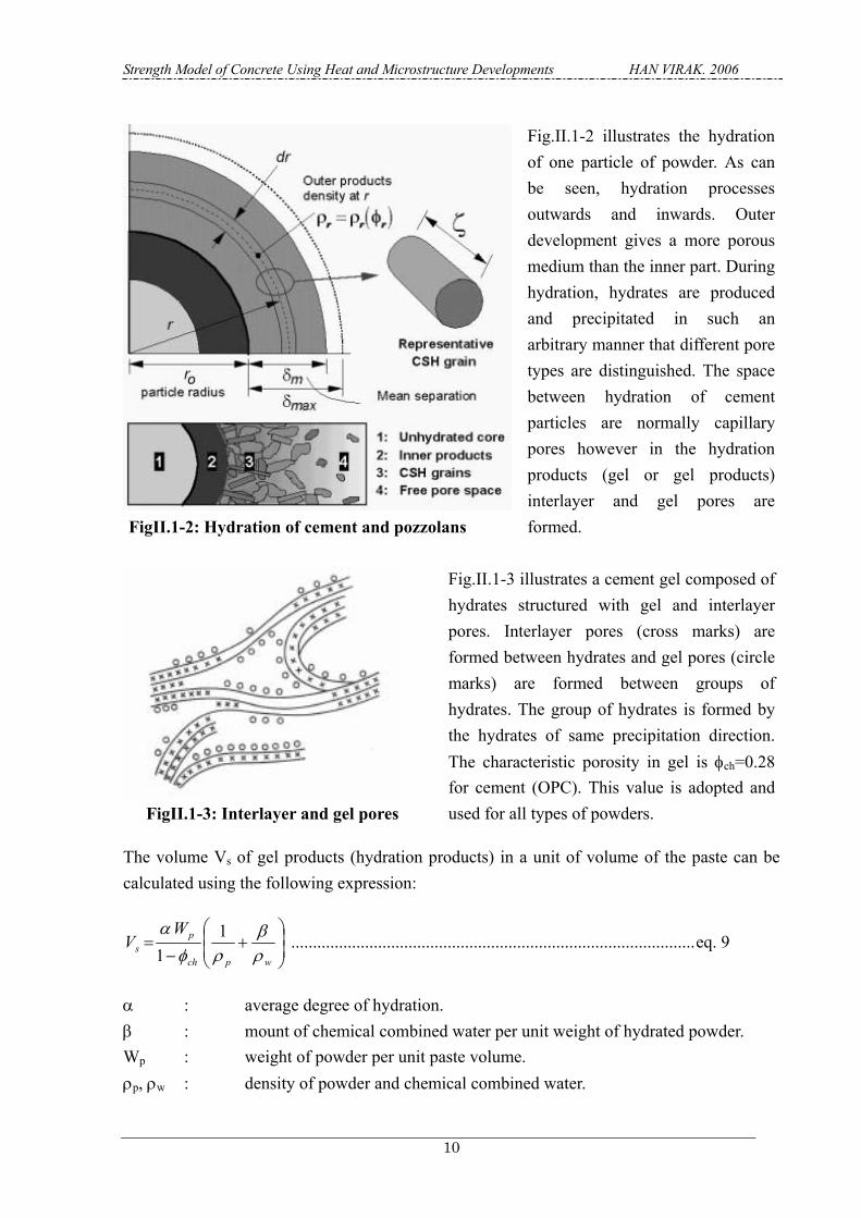
FigII.1-2: Hydration of cement and pozzolans
Fig.II.1-2 illustrates the hydration of one particle of powder. As can be seen, hydration processes outwards and inwards. Outer development gives a more porous medium than the inner part. During hydration, hydrates are produced and precipitated in such an arbitrary manner that different pore types are distinguished. The space between hydration of cement particles are normally capillary pores however in the hydration products (gel or gel products) interlayer and gel pores are formed.
FigII.1-3: Interlayer and gel pores
Fig.II.1-3 illustrates a cement gel composed of hydrates structured with gel and interlayer pores. Interlayer pores (cross marks) are formed between hydrates and gel pores (circle marks) are formed between groups of hydrates. The group of hydrates is formed by the hydrates of same precipitation direction. The characteristic porosity in gel is φch=0.28 for cement (OPC). This value is adopted and used for all types of powders.
The volume Vs of gel products (hydration products) in a unit of volume of the paste can be calculated using the following expression:
+
−=
wpch
ps
WV
ρβ
ρφα 11
.............................................................................................eq. 9
α : average degree of hydration. β : mount of chemical combined water per unit weight of hydrated powder. Wp : weight of powder per unit paste volume. ρp, ρw : density of powder and chemical combined water.

Strength Model of Concrete Using Heat and Microstructure Developments HAN VIRAK. 2006
11
The interlayer porosity (φl) and gel porosity (φg) are calculated by eq.10 and eq.13
2/)( glwl st ρφ = .......................................................................................................eq. 10
tw : interlayer thickness (=2.8 Ao)-(Anstrom = 10-10m). lφ : is interlayer porosity per volume of gel product.
sl : specific surface area in (m2/g) and is calculated by eq.11
fasgpcl fffs 31001500510 ++= ..............................................................................eq. 11
fpc, fsg, ffa : weight fractions of cement, slag and fly ash.
The dry density of gel products is given by eq.12.
)()1)(1(
pw
chwpg βρρ
φβρρρ
+
−+= .......................................................................................eq. 12
The gel porosity is then deduced with eq.13
lchsg V φφφ −= ..........................................................................................................eq. 13
Finally, the capillary porosity is calculated by
)/)(1(1 ppsc WV ραφ −−−= ...................................................................................eq. 14
α , which is the degree of hydration which will be reviewed in the next section.
Some parameters that derive from interlayer, gel and capillary porosity are effective porosity and total porosity. The effective porosity (EP) is the sum of gel and capillary porosity on the other hand the total porosity is the sum of interlayer, gel and capillary porosities.
cgEP φφ += .............................................................................................................eq. 15
II.2. Multi-component heat model
The heat of hydration of cement and pozzolanic materials were the main topics in concrete engineering in order to model the development of cementitious materials. Many of models were proposed by different researchers, some were totally empirical and some others were very scientific. The multi-component heat model used in this research was proposed by Kishi et al. The model was based on the fundamental values (Hi,To) of heat rate of each cement

Strength Model of Concrete Using Heat and Microstructure Developments HAN VIRAK. 2006
12
component obtained from experiments [9]. The reference heat rate is function of accumulated heat. The total heat rate can be calculated by eq.16.
FAFASGSGSCSCSCSC
AFCAFETCAFCACAETCAC
iic
HpHpHpHpHHpHHp
HpH
+++++++=
=∑
2233
444333 )()( ...........................................eq. 16
Hi : heat generation rate of mineral i per unit weight pi : weight composition ratio. HC3AET, HC4AFET : heat rates in formation of ettringite.
The heat generation rate of each mineral compound was calculated with the proposed equation eq.17 which depended on the actual temperature, delaying effect, water reduction effect, effect of Ca(OH)2 lack, mineral interaction effect and fineness effect.
−−=
0,
11exp)(TTR
EQHsH i
iTiiii λµγβ ............................................................eq. 17
∫= dtHQ ii ..............................................................................................................eq. 18
Ei : activation energy of component i. R : gas constant. Hi,To : reference heat rate of component i at constant temperature To. γ : coefficient expressing the delaying effect of admixtures. βI : reduction coefficient in heat generation rate due to availability of free water. λ : change coefficient of heat generation rate of blast furnace slag and fly ash
due to the lack of calcium hydroxide. µ : change coefficient of heat generation rate in term of the difference of
mineral composition of Portland cement. si=Si/Sio: change coefficient of reference heat rate according to the fineness of
powders. -Ei/R : thermal activity which is determined by the experimental works.
• Reference Heat generation rate and thermal activity
The heat generation rate is calculated based on the reference heat generation rate measured on the clinker minerals of OPC. In this proposed scheme, the reference heat rates are represented

Strength Model of Concrete Using Heat and Microstructure Developments HAN VIRAK. 2006
13
with multiple breaking lines divided into typical stages of hydration including: dormant period, control process and diffusion control.
FigII.2-1: Reference heat generation rate of cement and pozzolans
Fig.II.2-1 shows the heat generation rate of cement compounds and pozzolans and the thermal energy as function of accumulated heats. In the heat model 2005, the thermal activities showed in the Fig.II.2-1 are changed to be constant. When this is used for cement of different compositions, the effect of compound interaction and micro filler effect must be taken into account. The modification factors of C2S and C3S are shown in Fig.II.2-2 and are represented by CHr
−−=
C
SC
SCCH p
pbarr
2
3max exp ..............................................................................eq. 19
where, b and c are respectively equal to 0.025 and 7.0. rmax and a are respectively 1.05 and 0.9 for alite case and 1.3 and 1.0 for belite case.

Strength Model of Concrete Using Heat and Microstructure Developments HAN VIRAK. 2006
14
FigII.2-2: Modification factor for heat generation rate due to mineral composition
According to Fig.II.2-2, C3S is much affected by C2S however C3S is less affect by C2S. The heat rate of C2S is much different between when C3S content is low and when C3S content is high.
After the heat rate is modified with the mineral composition effect, it must be rectified with the micro-filling effect which is calculated in the following equations:
)53()1(' ≤≤+= jHSrsHS jj ................................................................................eq. 20
)64(1
' maxmax ≤≤
+
−−= j
rsQQ
QQ jj ......................................................................eq. 21
FigII.2-3: Change of heat rates due to micro-filler effect
Fig.II.2-3 shows the change of heat rate due to the fact that cement particles are so fine that the filling effect occurs.

Strength Model of Concrete Using Heat and Microstructure Developments HAN VIRAK. 2006
15
+
−−=e
SCSC
SC
ppp
drsrs23
2max exp1 ................................................................eq. 22
where, rsmax, d and e are respectively 1.2, 3.0 and 5.0.
FigII.2-4: Thermal activity (modified 2005)
• Free water-missing effect
−−=
s
ii
freei s
wr 2/1/
100exp1
ηβ ........................................................................ eq. 231
r = 5 and s = 2.4 : material constants.
CWW
w itotalfree
∑−= ................................................................................................eq. 24
3/1
,
11
−−=
∞i
ii Q
Qη ..................................................................................................eq. 25
Where Wtotal : unit water content. Wi : water consumed and fixed by the reaction of constituents.
1 reference:[17] and [18]

Strength Model of Concrete Using Heat and Microstructure Developments HAN VIRAK. 2006
16
C : unit cement content. Qi : accumulated heat of component i.
∞,iQ : final heat generation.
In case that slag or fly ash is used separately or in combination, the free water reduction due to a shortage of Ca(OH)2 was taken in account and treated by eq.26.
( )FAFASGSGPC
itotalfree pmpmpC
WWW
... ++
−= ∑ .......................................................................eq. 26
iim βλ /= ................................................................................................................eq. 27
• Inter-dependence coefficient.
The inter-mineral interaction effect was considered to depend on the percentage of C3S and C2S which were believed to play a role in both heat and strength developments. According to Fig.II.2-5, the hydration stages other than stage 3 are not affected.
FigII.2-5: Inter-dependence effect
The following equation was proposed for the inter-dependence effect:
1.0.48.0exp14.14.1
2
3 +
−−=
SC
SC
pp
µ .................................................................eq. 28
• Coefficient of left and need of Ca(OH)2.
The reaction of slag and fly ash was reported to take place only with sufficient supply of Ca(OH)2 left by cement reaction. The reaction of cement is accompanied with release of Ca(OH)2 which is consumed by slag, fly ash and some other pozzolans. This shows that the

Strength Model of Concrete Using Heat and Microstructure Developments HAN VIRAK. 2006
17
prediction of hydration of pozzolans must be concerned with the factor controlling the supply and consumption of Ca(OH)2. As can be illustrated in Fig.II.2-6, fly ash consumes Ca(OH)2 from cement and retards cement hydration however, slag consumes without retarding. In ternary case, fly ash keeps playing its role as retarding agent. This retarding effect is reckoned in with the coefficient γ. When the Ca(OH)2 supply is reduced in the reaction medium, water availability is also affected then the free water-missing effect is to recalculate as in the section free water-missing effect.
The lack and need of Ca(OH)2 for pozzolanic reaction was accounted for by using the following equation:
+
−−=0.5
0.2exp1FACHSGCH
CH
RRF
λ .....................................................................eq. 29
FCH : is the amount of Ca(OH)2 produced by C3S and C2S and not yet consumed by C4AF.
RSGCH and RFACH : is the amount of Ca(OH)2 necessary for reaction of slag and fly ash.
FigII.2-6: Connection between heat rates of blast furnace slag and fly ash with OPC
• Effective Delaying coefficient.
When a super-plasticizer (SP) was used, the delaying effect short or long was sure to occur.
Strength Model of Concrete Using Heat and Microstructure Developments HAN VIRAK. 2006
18
The effective SP was calculated by eq.31 then the delay coefficient was proposed by eq.30.
++
+−=
SGSGSCSCSCSC
FAefSPef
spspsp 5,2510)(1000
exp2233
ϑϑγ ....................................................eq. 30
γ : delaying coefficient of heat generation reduction in stage 1.
WasteSPSPSPef p υχυ −= . ............................................................................................eq. 31
)5416(2001
4433 FAFASGSGAFCAFCACACWaste spspspsp +++=ϑ ..................................eq. 32
Wasteϑ : Effect of chemical admixtures without influencing the delay.
efϑ : Effective delaying capability.
SPχ : Coefficient representing the delaying effect per unit weight of admixture.
Table II.2-1: Delaying effect corresponding to each type of admixtures
Main component of admixtures SPχ
Naphtalene sulfonate 1.2 Polycarboxilate 1.2 Air entraining agent 5
pSP : Dosage of organic admixture expressed as additive ratio to binder (Cx%)
FAFAFAef sp.2.0=ϑ ....................................................................................................eq. 33
After heat generation rate is calculated, the average degree of hydration is given by:
∑∞
=i i
ii Q
Qp .α ..........................................................................................................eq. 34
The process of calculation hydration heat on one age is to make summations of hydration of all time steps. As can be shown in Fig.II.2-7, the process begins with an initialization of accumulated heat. At zero time, accumulated heat is zero, but the reference heat rate is not
zero. Hi,To and REi are calculated from Fig.II.2-1 and at the same time ii s,,,, µλβγ can
be calculated. The heat rate is then calculated. By multiplying with the initial time step, the

Strength Model of Concrete Using Heat and Microstructure Developments HAN VIRAK. 2006
19
increase of heat can be known and the new heat is accumulated, this new accumulation of heat is used for determining the reference heat rate of the next loop.
FigII.2-7: Hydration heat calculation process
II.3. Porosity measurement and the disadvantages
Paste is hardened progressively with time during reaction of cement with water. At the same time that cement particles are reacted, the paste becomes compacted and strong by interlacing cement particles with outside hydrates. The structure of hardened pastes is complex because of the complexity of forms of different types of hydration products including CSH2, CH3, AFm (alumino-ferrite mono), AFt (alumino-ferrite tri) and others. Jennings et al. reported that CSH possessed 4 main forms including CSH type I, II, III and IV. These CSH types exist in cement paste in some stages of hydration and are foil-like and fibrillar. CH, AFm and AFt have similar layer structures. Pore structures are not of fixed forms but determined by the hydrate products which are foils and fibrillar and which are interlocked. The knowledge of porosity becomes interesting since it determines many properties of concrete. Porosity and porous structures were measured with several methods among which MIP (mercury intrusion porosimetry) meets wide applications. The microstructure development model used in calculating pores in this research was established basing on MIP. So it is essential to know how fine pores can be measured with MIP. The method was based on the fact that mercury does not wet a porous solid will enter pores only under pressures. Washburn assumed that pores are cylindrical and calculated the pressure p
2 Calcium silicate hydrate: tobermorite (C5S5.5H9), CSH type I (C5S5H6), Jennite ( C9S6H11) and CSH type II (C9S5H11). C=CaO; S=SiO2 and H=H2O. 3 Calcium hydroxide: Ca(OH)2 or Portlandite.
Initial step Qi = 0 Step = 0.015
Heat rate Hi Accumulated heat Qi
−−=
0,
11exp)(
TTRE
QHsH iiToiiii λµγβ
i represents the compound: C3A, C4AF, C2S, C3S, Slag and fly ash.
Degree of hydrationPorosity
ti+1 = ti + dt

Strength Model of Concrete Using Heat and Microstructure Developments HAN VIRAK. 2006
20
needed to place in pores of diameter d by /dcosθγ4p −= where θγ; are respectively the surface energy of liquid (Hg=0.483Nm-1) and the contact angle (117o-140o). Even MIP is widely applied; we should pay strict attentions to the disadvantages happening in some cases. The followings are some problems not resolved yet by researchers (Taylor. H. F. W, Cement Chemistry, 2nd edition, 1997, pp. 248-249).
1. The method does not measure the distribution of pore sizes, but that of pore-entry sizes (Dullien, 1979). If large pores can be entered only through small pores, they will be registered as small pores. Previous suspicions that this effect is of major significance with cement pastes were supported by the results of computer modeling of the entry of mercury into cement pastes (Garboczi, 1991).
2. The delicate pore structure of the paste is altered by the high stress needed to intrude the mercury. This effect was shown in studies on composite cements, in which mercury was intruded, removed and re-intruded into mature pastes. Contrary to earlier conclusions, it also occurs with pure Portland cement pastes (Feldman, 1991).
3. As with other methods in which the paste has first to be intensively dried, the pore structure is also altered by the removal of the water. Isopropanal replacement followed by immediate evacuation and heating at 100oC for 2h has been reported to cause the least damage (Feldman, 1991).
4. It is not clear whether the method registers the coarsest part of the porosity, intruded at low applied pressures.
5. The assumption of cylindrical pores and of a particular contact angle may be incorrect.
According to these above cited remarks, the real porosity is coarser than the one given by MIP.
When slag and fly ash are used, they can react with Ca(OH)2 released from cement hydration and the reaction leads in general to a low Ca/Si ratio and Ca(OH)2 are replaced with CSH. Harrison (1987), Regourd (1986) and Uchikawa (1986) concluded that the microstructures of slag cement pastes were similar to those of Portland cement paste apart from the lower CH content. Harrison continued that the similarity between slag cement pastes and Portland cement pastes were typical for fly ash-cement pastes. Basing on the TEM (Transmission Electron Microscope) these microstructures changed from fibrillar shapes to foil-like shapes which allowed slag-cement pastes to have lower permeability than cement paste (Regourd, 1992). Most researchers shared their opinion about the difficulties found in studying pore structures of composite cements using mercury intrusion due to the foil-like shapes with fine entry sizes of pore.
Strength Model of Concrete Using Heat and Microstructure Developments HAN VIRAK. 2006
21
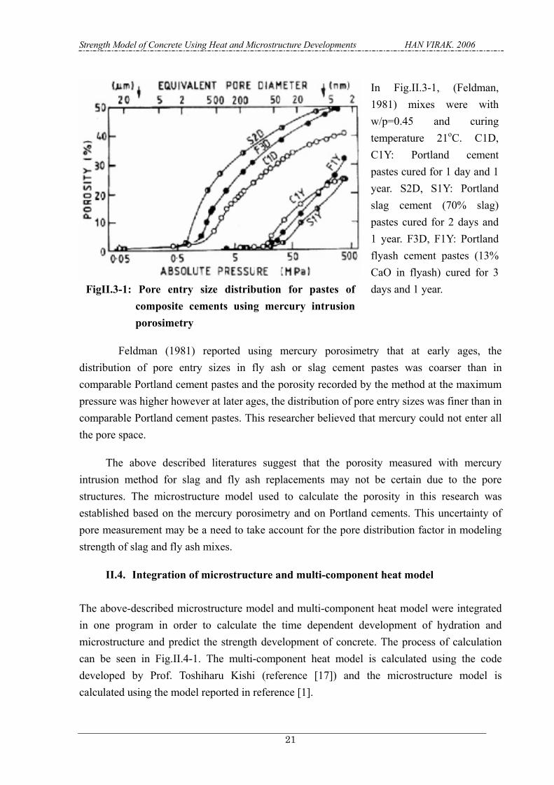
FigII.3-1: Pore entry size distribution for pastes of
composite cements using mercury intrusion porosimetry
In Fig.II.3-1, (Feldman, 1981) mixes were with w/p=0.45 and curing temperature 21oC. C1D, C1Y: Portland cement pastes cured for 1 day and 1 year. S2D, S1Y: Portland slag cement (70% slag) pastes cured for 2 days and 1 year. F3D, F1Y: Portland flyash cement pastes (13% CaO in flyash) cured for 3 days and 1 year.
Feldman (1981) reported using mercury porosimetry that at early ages, the distribution of pore entry sizes in fly ash or slag cement pastes was coarser than in comparable Portland cement pastes and the porosity recorded by the method at the maximum pressure was higher however at later ages, the distribution of pore entry sizes was finer than in comparable Portland cement pastes. This researcher believed that mercury could not enter all the pore space.
The above described literatures suggest that the porosity measured with mercury intrusion method for slag and fly ash replacements may not be certain due to the pore structures. The microstructure model used to calculate the porosity in this research was established based on the mercury porosimetry and on Portland cements. This uncertainty of pore measurement may be a need to take account for the pore distribution factor in modeling strength of slag and fly ash mixes.
II.4. Integration of microstructure and multi-component heat model The above-described microstructure model and multi-component heat model were integrated in one program in order to calculate the time dependent development of hydration and microstructure and predict the strength development of concrete. The process of calculation can be seen in Fig.II.4-1. The multi-component heat model is calculated using the code developed by Prof. Toshiharu Kishi (reference [17]) and the microstructure model is calculated using the model reported in reference [1].

Strength Model of Concrete Using Heat and Microstructure Developments HAN VIRAK. 2006
22
FigII.4-1: Integration of multi-component heat and
microstructure models
Microstructure Model
• Hydration Heat of C2S, C3S, C3A, C4AF, Slag, FA
• Degree of hydration
• Porosity: interlayer , gel and capillary porosity
• Effective porosity
Strength Prediction Model
Multi-component Heat Model

Strength Model of Concrete Using Heat and Microstructure Developments HAN VIRAK. 2006
23
CHAPTER III: METHODOLOGY III. Methodology
The main concern of research was strength which had to be tested for mixes whose properties were calculated. Many researchers believed that compressive strength of concrete depends on raw material compositions and strength testing. The latter is influenced by several operational factors such as the loading rate, moisture condition, curing conditions, specimen size, machine platen size and others. Consequently, the procedures were described in the following in order to specify what has been done and to assure the quality of the authors' results.
III.1. Materials
Raw materials used in mortar or concrete production can be found in many areas where the physical and mechanical properties are quite different. Natural, industrial materials and waste can be used as components of concrete. The natural materials are sand exploited from river, sea or mountains. The industrial materials are cement, produced ash and the waste materials are blast furnace slag, fly ash, plasticizers and super-plasticizers.
III.1.A. Admixtures
Admixtures are defined as materials added to concrete before, during mixing or immediately before placing in order to improve the physical and chemical properties of paste or concrete which eventually affects the mechanical property in both short and long-term durability. According to functions offered, admixtures are categorized in ASTM C494-98 into 7 types:
• A (water-reducing admixtures),
• B (retarding admixtures),
• C (accelerating admixtures),
• D (water-reducing and retarding admixtures),
• E (water-reducing and accelerating admixtures),
• F (water-reducing, high range admixtures) and
• G (water-reducing, high range and retarding admixtures).
Among these admixtures, super-plasticizers (SP) (types F and G) become very popular because it offers a variety of flexibility to settle many concrete problems ranging

Strength Model of Concrete Using Heat and Microstructure Developments HAN VIRAK. 2006
24
from fresh workability to long-term durability. An example of workability improvement was the production of self-compacting concrete and an example of long-term durability was the production of high performance concrete by incorporating silica fume. This very interesting capacity was due to its fundamental mechanism in dispersing cement particles by three ways such as an increase of ς -potential, an increase of solid-liquid affinity and steric hindrance (Daimon, 1978). These three effects can be high or low depending on the types of SP including sulfonated melamine formaldehyde polymers (poly(melamine sulfonate); MS), sulfonated naphthalene formaldehyde polymers (poly(naphtalene sulfonate); NS), lignosulfate materials and polycarboxylate based superplasticizers. The dispersing mechanism of the polycarboxylate types was reported based on the steric hindrance and the dispersion increased as the polymer length or the absorption thickness increased (Sakai, 2003). In this research, cement and other powders have to be well dispersed in order to simulate mixes as ideal as in the microstructure and multi-component heat models, therefore super-plasticizers were used as admixture. SP are not only good dispersing agents but are also set delayers and air-entrainers. According to Suzuki, the delaying effect varies according to the type of SP. SP used was RHEOBUILD SP8SB_Sx2 which was made of compounds of polycarboxylate ether with their cross-linked polymers. It had a density of 1.04 g/cm3 and a pH of 9. This type of SP was the same type used by Suzuki in his experiment and according to his report, the delaying effect was 1.2.
III.1.B. Cements
Cement is defined as hydraulic powder which can react with water and harden under water to form a hardened rock. Cement, according to its manufacturing process, is an expensive powder among powders used in concrete engineering. Cement compositions are not unique however are variable due to sources of raw materials and production purposes. In concrete, cement is the first component that reacts with water; its reaction is always accompanied with hydration heat whose value may be high or low according to the cement components mainly including: C2S, C3S, C3A, C4AF and gypsum. Strength of cement is of first importance because its role is to bond all aggregate together to form a unique rock. In Japan, low heat Portland cement is pure cement; it is selected for use in the first investigation to find the ideal mixes prescribed by the microstructure and multi-heat component models.
After determining some effective parameters which have a close influence on strength, these parameters have to be studied and modeled with the strength tested on the specimens. The model has to be applied with different types of cement characterized with the composition of C2S, C3S, C3A and C4AF. The properties and compositions of these cements were listed as following:

Strength Model of Concrete Using Heat and Microstructure Developments HAN VIRAK. 2006
25
Table III.1.B-1: Cement compositions
Percentage by weight Mineral types LH (Low
heat) HES (High
Early Strength) OPC (Ordinary
Portland Cement)C3S (tricalcium silicate or alite) 28 63 58 C2S (dicalcium silicate or belite) 53 11 15.5 C3A (tricalcium aluminate) 3 9 11.4 C4AF (tetracalcium ferro-aluminate
or ferrite) 10 8 7.6
Physical properties Specific gravity in g/cm3 3.24 3.13 3.13 Surface area in cm2/g 3280 4770 3400
III.1.C. Powders
Defined as powders, all materials finer than 0.075 mm they can be hydraulic, pozzolanic, latent hydraulic. Many powders are available for concrete production. They are used to enhance the fresh (flowability, bleeding retention) and hardened properties (strength, durability) of concrete. Powders excluding cement have been broadly categorized as pozzolanic or latent hydraulic. Neither type reacts significantly with water at ordinary temperature in absence of Ca(OH)2 supply. Pozzolanic powders are always low in CaO and high in Si2O or Al2O3, they react with water and CaO supplied by cement reaction and finally give hydration products of low Ca(OH)2 even the structure is almost the same as pure hydraulic cement products. Included in this type, are fly ash class F, natural pozzolana and silica fume. However, latent hydraulic powders have reaction property between hydraulic cements and pozzolanic materials and can react consuming a minimal amount of catalyst or activator. In general, latent hydraulic powders can be used in higher amount than pozzolanic powders to replace some cement. Considered as latent hydraulic, are slag and fly ash class C. Another powder which is neither pozzolanic nor latent hydraulic is finely ground limestone. This powder becomes now very interesting in concrete technology as cement replacement powder. In this paper, the authors also included the often-used powders in the investigation. Those powders are listed in Table III.1.C-1. The blast furnace slag is slag from factory it is not mixed with other compounds of clinker. All the powders are blended with low heat cement when batching. The replacement ratio of a powder is defined as the ratio of that powder weight to the total weight of all powders. This replacement ratio is used to identify a fraction of the powder in powder composition.

Strength Model of Concrete Using Heat and Microstructure Developments HAN VIRAK. 2006
26
Table III.1.C-1: Powder properties
Limestone Fly ash (II)4 Blast furnace slag Specific gravity (g/cm3) 2.7 2.36 2.91 Fineness modulus (g/m2) 3530 3410 3930
III.1.D. Sands
Sand is defined as an aggregate whose grain sizes ranges from 0.075 mm to 5 mm. These materials can be composed of various minerals which provide specifically a diversity of physical and mechanical properties. In concrete, despite of the reactivity of some minerals with cement, sand is considered as an inert component that may affect the resulted mix property by its texture, size, sieving distribution, strength and other secondary properties. In general, sand contains water some of which is absorbed inside and some other is attached to surface. The inside absorbed water content with dry surface is called SSD water content or water absorption content, on the other hand the water content attached to surface is called surface free water. The latter is a cause of variation of mix properties because of its downward movement which makes the water content non-uniform. In order to keep water content of sand uniform, sand need to be kept with water content the same as SSD water content. Of course, sand ordered from suppliers had water content variable and different from SSD water content, so the preparation of a large required quantity was indispensable.
Table III.1.D-1: Sand properties
First sand Second sand Bulk SSD specific gravity 2.57 2.59 Apparent specific gravity 2.64 2.67 Absorption 1.86 1.87 Fineness modulus 2.75 2.97
The preparations was really troublesome but was successfully managed using the following methods. First, sand was sampled and tested for SSD water content according to ASTM C-128-97. Second, an amount equal to the container volume was taken and stirred with a concrete mixer and then the actual water content was checked with a moisture meter. Third, if the actual water content was higher than the SSD water content, sand had to be dried. Fourth, if the actual water content was lower than the SSD water content, the amount of water needed to add in order to make the whole sand become at SSD condition was calculated and added and finally sand was uniformly stirred. Fifth, sand was inserted into the storage 4 Fly ash type II, Japanese product.

Strength Model of Concrete Using Heat and Microstructure Developments HAN VIRAK. 2006
27
container and kept in the control room with a regular check. The storage condition was shown in Fig.III.1.D-2.
Coarse sands' sieving curve
0%10%20%30%40%50%60%70%80%90%
100%
1 2 3 4 5 6 7 8 9 10 11 12 13 14 15 16 17
Nominal Sieve size
Pass
ing
First sand Second sand
0.075 0.3 1.2 5 15 25 40 60 100 0.15 0.6 2,5 10 20 30 50 80
Fig III.1.D-1: Sieving curve of crushed sands
In this experimental works, sand as well as other materials were prepared and kept in a room with well-controlled conditions. The room condition was always maintained at temperature 20oC and at RH=60%. In this condition, the remarkable problem was the early evaporation of water from sand at the top part of the storage containers and the non-uniform water content was observed between the top and the bottom of sand container.
Fig III.1.D-2: Storage condition of sand
Sand
Container
Wet cloths
Plastic sheets
Cover

Strength Model of Concrete Using Heat and Microstructure Developments HAN VIRAK. 2006
28
A solution was to put two separate sheets of plastic between which exist some wetted cloths at the top of sand. This solution allows keeping sand for a long time without changing its water content but cares had to be taken to prevent the wetted cloths from drying.
III.2. Mixer and mixing
Mixer is an apparatus in which materials of different types are uniformly mixed. The mixers are classified into 2 main types: batch mixers and continuous mixers. The first type produces concrete one batch at a time and the second type produces concrete at a constant rate. The mixer and mixing method are effective contributions to the concrete performance. Fig.III.2-1 shows the shape of the mixer used in this research. The mixer was a fixed cylinder inside which, there were 3 spatulas that turned around the axis of the cylinder. The maximum volume that can be mixed is 50 liters however all mixes were conducted with only 22 liters (for 12 specimens).
Fig III.2-1: Mixer
Mixing is an operation in which three stages including loading, mixing and discharging are successfully completed. In loading stage, some components are introduced in an order which is believed to affect good concrete properties. Mixing can be divided into dry mixing and wet mixing. Paillere (1990) concluded that the delayed addition of high range water reducer admixture (HRWRA) leads to a better dispersion of cement. So in order to achieve good dispersion, super-plasticizer was input one minute after water introduction. Cares should be taken during discharge in order to prevent segregation. Before mixing, all the necessary materials were correctly dosed and kept aside the mixer with covers to prevent eventual evaporation or desiccation. ASTM C192 suggests that a plastering mix of the same proportion as the main mix should be made in order to compensate the effect of material consumption by
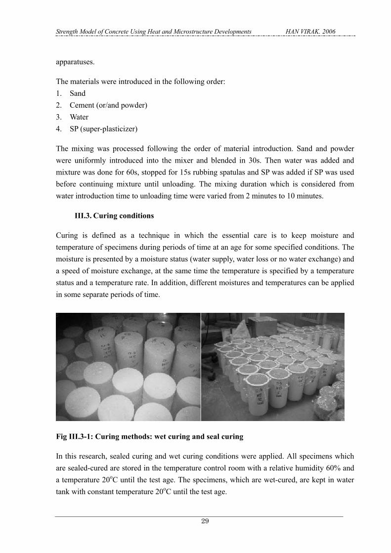
Strength Model of Concrete Using Heat and Microstructure Developments HAN VIRAK. 2006
29
apparatuses.
The materials were introduced in the following order: 1. Sand 2. Cement (or/and powder) 3. Water 4. SP (super-plasticizer)
The mixing was processed following the order of material introduction. Sand and powder were uniformly introduced into the mixer and blended in 30s. Then water was added and mixture was done for 60s, stopped for 15s rubbing spatulas and SP was added if SP was used before continuing mixture until unloading. The mixing duration which is considered from water introduction time to unloading time were varied from 2 minutes to 10 minutes.
III.3. Curing conditions
Curing is defined as a technique in which the essential care is to keep moisture and temperature of specimens during periods of time at an age for some specified conditions. The moisture is presented by a moisture status (water supply, water loss or no water exchange) and a speed of moisture exchange, at the same time the temperature is specified by a temperature status and a temperature rate. In addition, different moistures and temperatures can be applied in some separate periods of time.
Fig III.3-1: Curing methods: wet curing and seal curing
In this research, sealed curing and wet curing conditions were applied. All specimens which are sealed-cured are stored in the temperature control room with a relative humidity 60% and a temperature 20oC until the test age. The specimens, which are wet-cured, are kept in water tank with constant temperature 20oC until the test age.

Strength Model of Concrete Using Heat and Microstructure Developments HAN VIRAK. 2006
30
III.4. Testing methods
Real compressive strength is obtained when a specimen is ruptured under uniaxial loading and fracture types are columnar, this happens to the case of free effect of end restrain between specimen surfaces and the machine platens however in practices, the often rupture type is conical. This means that conventional strength tested is not real but lower compared to the real strength. The following shows how strength testing is affected by other factors.
III.4.A. Sampling, specimen size and age
After unloading mortar, slump or slump flow were measured then poured into moulds. The moulds were cylindrical of 100 mm diameter and 200 mm height and made of plastics.
Some researchers had investigated the effect of specimen size on strength and gave some useful conclusions. Gonnerman, H.F (1925) claimed that the compressive strength of concrete decreased with the increase of specimen size. Neville, A.M. (1987) identified rupture types affected by platen size and specimen size due to the platen restrain. The cylinder is a better specimen than a cube because of less end restrain and more uniform distribution of stress. According to some technical reports, the smaller specimen size would induce the higher platen restrain which increased the difference between the conventional strength and the real strength however the specimen of high strength must have a limited size because of limit of machine capacity. Owing to the restriction of machine capacity and the ability to obtain the least end restrain, the cylinder100x200 should be decided.
3 specimens were sampled for one age of strength test. The 7th day and 28th day ages were used for series of mixes conducted for investigating sand content effect, dispersion effect and mixing time effect. These series were fundamental experimental works because they were used to investigate the ideal condition of mixes and then to determine the mixes which had components dispersing almost in the same manner as assumed in the microstructure and multi-heat models. The ages 7th, 14th, 28th and 91st days were used for strength modeling whose purpose was to be able to predict both early and long-term strengths.
III.4.B. Surfacing
End surfaces of a specimen have to be horizontal and perpendicular to the axe of the specimen during strength testing. The inclination of end surfaces were believed to cause the deviation of strength values among a set of 3 specimens and give a value lower than the real one. Three methods have been often reported effective in avoiding the effect of friction between end surfaces and the platens. This effect affected the rupture type and strength. The first method is

Strength Model of Concrete Using Heat and Microstructure Developments HAN VIRAK. 2006
31
to use pure sulfur, a sulfur-sand mix or early strength mortar to cap both end surfaces of specimen. Due to the strength limit of capping materials, the method is suitable for normal strength testing. The second method is to use a bearing cap which can remove the friction by simply putting between the specimen surface and the platen. The third method in which a grinder machine is used to grind the end surfaces can be simply and reliably operated. According to some experienced engineers, the comparison among the 3 methods shows that the third one is the most reliable and suitable in this research. The grinder machine, as can be seen in Fig.III.4.B-1, can be used to grind three specimens at a time however in this experimental works, one specimen at a time was ground because some workers reported that grinding 3 specimens at a time would not offer a horizontal plane surface. Both top and bottom surfaces of specimens were ground.
Fig III.4.B-1: Grinder machine
III.4.C. Compressive strength test
Shimadzu Testing Machine was used to test compressive strength. The machine has a capacity of 1000 kN which corresponds to the possible maximum stress of 127 MPa as 100x200 cylinders were used. The test operation was ordered with an automatic mode and a constant stress speed of 0.21MPa/sec that was in the range recommended by ASTM-C39-96 standards. This stress speed was kept constant for all tests. Specimens were placed centrally onto the bottom plate carved with central guidelines. The top plate was then slowly moved downward to contact the specimen top surface. The specimen was covered with a security cylindrical cover to protect exploded debris. When preparation was ready, loading was started. One

Strength Model of Concrete Using Heat and Microstructure Developments HAN VIRAK. 2006
32
strength point was the average of three specimens which showed a small deviation.
Fig III.4.C-1: Universal testing machine

Strength Model of Concrete Using Heat and Microstructure Developments HAN VIRAK. 2006
33
CHAPTER IV: MIX PROPORTIONING IV. Mix proportioning
The mix proportion is the first operation taken in a mix design which is aimed to find a proportion correspondent to an imposed requirement including fresh properties (workability) and hardened properties (strength and durability). It is aimed only to calculate quantities of all components. Basing on one cubic volume balance, a mix proportion must respect to eq.35.
1VVVVV gSCWV =+++++ PV ..........................................................................eq. 35
Where the indexes V, W, C, P, S and g represent respectively void, water, cement, powder, sand and coarse aggregate.
IV.1. Fundamental proportioning
The mix proportion is defined in the manner that all components form one cubic meter, so the amount of a component depends on the others. If one component increases (decreases), another or others decrease (increase).
The following symbols are used for fundamental mix proportioning: a) w/c: this is believed to play an important role in strength development
and porosity. The higher w/c, the more porous and then the weaker strength. b) w/p: the water-powder ratio is used instead of w/c when powder other
than cement is used. Even powder is not reactive (latent-hydraulic or pozzolanic), the presence of powder increases degree of hydration by giving more surface area.
c) W: water content is an important index for workability, strength and durability.
d) s/a: this is a ratio of sand in volume compared to total aggregate volume (sand and coarse aggregate), it is defined basing either on strength or workability. This is equal to 0.45 for the best workability with Japanese materials. It can also be defined basing on many other methods including: Bolomey, Fuller, Faury…These methods aim to determine a ratio s/a with a proposed optimum line considering that sand-aggregate will give a mix with

Strength Model of Concrete Using Heat and Microstructure Developments HAN VIRAK. 2006
34
less porosity. s/a can be calculated numerically using packing density theory proposed by Francois De Larrard (1999) [3].
Symbols for Physical properties and compositions - ρc: specific gravity of cement in g/cm3. - ρs: specific gravity of sand in g/cm3. - ρg: specific gravity of coarse aggregate in g/cm3. - ρpi: specific gravity of powder i in g/cm3. - Rpi: replacement ratio of powder i in weight. - w/p: water-powder ratio in weight. - w/c: water-cement ratio in weight. - W: water content in kg. - C: cement weight in kg - P: total powder weight in kg including cement. - Pi: weight of powder i in kg excluding cement. - VPi: volume of powder i in m3. - S, G: sand and coarse aggregate weight respectively in kg - pa: assumed entrapped air in %. - s/a sand-aggregate ratio in volume.
Using the equation (35), the proportion is calculated either by weight or by volume; the following is given in weight:
In case that only cement is used as powder,
The known parameters are: W, w/c, s/a, pa, and physical properties of concerned materials. The unit of weight is in kg and that of volume is in m3.
)/(WC
cw= ; C)./(W cw= .....................................................................................eq. 36
−−−=
cs 1000.ρ
C1000
W100
1.ρ.1000)./(S apas .......................................................eq. 37
−−−−=
cg 1000.ρ
C1000
W100
1.ρ.1000))./(1(G apas ..............................................eq. 38
In case that other powders are used with cement,

Strength Model of Concrete Using Heat and Microstructure Developments HAN VIRAK. 2006
35
)/(WP
pw= ; P)./(W pw= ....................................................................................eq. 39
++
−−−= ∑∑ pw
pas a /
1000.ρR
1000.ρR1
.P100
1.ρ.1000)./(Spi
pi
C
pis .......................eq. 40
++
−−−−= ∑∑ pw
pas a /
1000.ρR
1000.ρR1
.P100
1.ρ.1000))./(1(Gpi
pi
C
pig ..............eq. 41
pii P.RP = ; pi
ipi 1000.ρ
PV = ......................................................................................eq. 42
∑−= iPPC ; C
piC 1000.ρ
R1P.V ∑−= ..........................................................................eq. 43
IV.2. Mortar in concrete
As coarse aggregate affects strength of concrete by its size, texture and strength so in order to avoid the coarse aggregate effect, it should be extracted, the mix becomes then a mortar. In this paper, mortar mixes which were used are all calculated by taking from concrete of normal ranges. A pair of concrete and mortar was defined basing on the same void percentage between concrete and mortar. To define a pair concrete-mortar, the composition diagram on Fig.IV.2-1 was drawn.
Symbols VC: unit volume of cement in concrete VS: unit volume of sand in concrete VG: unit volume of coarse aggregate in concrete C: unit weight of cement in concrete CM: unit weight of cement in mortar S: unit weight of sand in concrete SM: unit weight of sand in mortar Pi: unit weight of powder i in concrete PiM: unit weight of powder i in mortar VPi: unit volume of powder i in concrete VPiM: unit volume of powder i in mortar W: unit water in concrete WM: unit water in mortar

Strength Model of Concrete Using Heat and Microstructure Developments HAN VIRAK. 2006
36
Fig IV.2-1: Representation of components of a pair concrete-mortar (C-M)
In case that only cement is used From concrete to mortar, the following formulae are used:
100/V1100/1
VVCA
SSMa
a
pp−−
−= ...................................................................................eq. 44
100/V1100/1
VVCA
CCMa
a
pp−−
−= ...................................................................................eq. 45
From mortar to concrete, the following formulae are used:
1000W
1000.ρC
.1000(s/a)ρS
100/1VV
M
C
M
S
MCMC
++
−= ap
............................................................eq. 46
1000W
1000.ρC
.1000(s/a)ρS
100/1VV
M
C
M
S
MSMS
++
−= ap
.............................................................eq. 47
−−−−=
1000W
1000.ρC100/1)./(1V
CG apas .....................................................eq. 48
In case that powders other than cement are used
From concrete to mortar, the following formulae are used:
VG
VS
VP
VW
VV
VSx
VPx
VWx
VVx
pa=Vv pa=x
Vx
VV
pa=Vv
VSM
VPM
VWM
VV
Mortar Vx
Matrix Vmx C
oncr
ete
1m3
Mor
tar 1
m3

Strength Model of Concrete Using Heat and Microstructure Developments HAN VIRAK. 2006
37
100/V1100/1
VVCA
SSMa
a
pp−−
−= ...................................................................................eq. 49
100/V1100/1
VVCA
CCMa
a
pp−−
−= ...................................................................................eq. 50
100/V1100/1
VVCA
PiPiMa
a
pp−−
−= ..................................................................................eq. 51
From mortar to concrete, the following formulae are used:
1000W
1000.ρP
1000.ρC
.1000(s/a)ρS
100/1VV
M
Pi
iM
C
M
S
MCMC
+++
−=
∑ap
......................................eq. 52
1000W
1000.ρP
1000.ρC
.1000(s/a)ρS
100/1VV
M
Pi
iM
C
M
S
MPiMPi
+++
−=
∑ap
.....................................eq. 53
1000W
1000.ρP
1000.ρC
.1000(s/a)ρS
100/1VV
M
Pi
iM
C
M
S
MSMS
+++
−=
∑ap
......................................eq. 54
−−−−−= ∑ 1000
W1000.ρ
P1000.ρ
C100/1)./(1VPi
i
CG apas ..............................eq. 55
In the data discussion, the authors use the notation type xM-CWy-SPz which means the mortar taken (by calculation) from concrete of w/p=x, water content=y and SP dosage=z. For example, 0.3M-CW210-SP06 means the mortar in concrete of w/p=0.3, water content = 210 liters and SP dosage=0.6%.
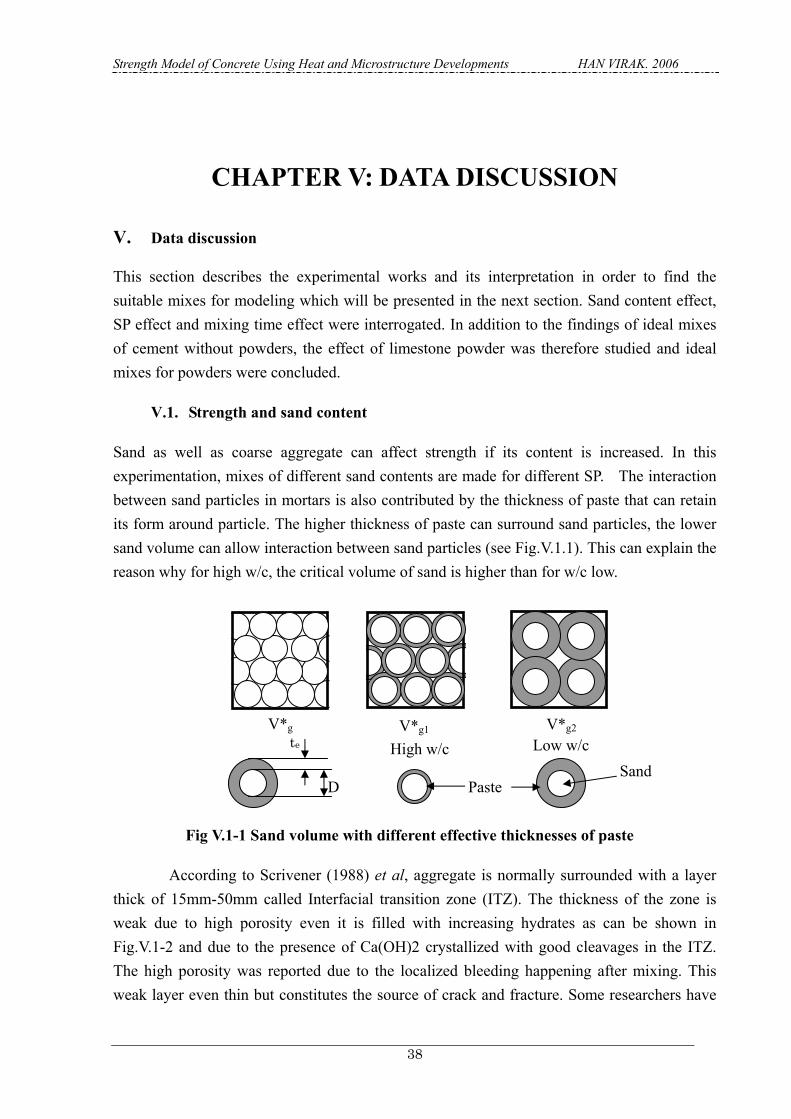
Strength Model of Concrete Using Heat and Microstructure Developments HAN VIRAK. 2006
38
CHAPTER V: DATA DISCUSSION V. Data discussion
This section describes the experimental works and its interpretation in order to find the suitable mixes for modeling which will be presented in the next section. Sand content effect, SP effect and mixing time effect were interrogated. In addition to the findings of ideal mixes of cement without powders, the effect of limestone powder was therefore studied and ideal mixes for powders were concluded.
V.1. Strength and sand content
Sand as well as coarse aggregate can affect strength if its content is increased. In this experimentation, mixes of different sand contents are made for different SP. The interaction between sand particles in mortars is also contributed by the thickness of paste that can retain its form around particle. The higher thickness of paste can surround sand particles, the lower sand volume can allow interaction between sand particles (see Fig.V.1.1). This can explain the reason why for high w/c, the critical volume of sand is higher than for w/c low.
Fig V.1-1 Sand volume with different effective thicknesses of paste
According to Scrivener (1988) et al, aggregate is normally surrounded with a layer thick of 15mm-50mm called Interfacial transition zone (ITZ). The thickness of the zone is weak due to high porosity even it is filled with increasing hydrates as can be shown in Fig.V.1-2 and due to the presence of Ca(OH)2 crystallized with good cleavages in the ITZ. The high porosity was reported due to the localized bleeding happening after mixing. This weak layer even thin but constitutes the source of crack and fracture. Some researchers have
Low w/c te
D
V*g V*g1 V*g2 High w/c
PasteSand

Strength Model of Concrete Using Heat and Microstructure Developments HAN VIRAK. 2006
39
been interested in producing high strength and durable concrete by improving the ITZ with incorporation of silica fume. Bentur (1988) concluded that partial replacement of cement by silica fume increases strength in concrete but not in pastes. This shows that the ITZ has certainly an effect on strength.
Fig V.1-2 Interfacial transition zone properties
As can be shown on Fig.V.1-3, two parts are distinguished, one is for sand volume less than 0.37 and another is for sand volume more than 0.37. Each line represents a series of mixes with one SP dosage corresponding to one level of dispersion. Sand effect plays different roles when the mix is at good dispersion, sand effect decreases strength however when the mix is at low dispersion, sand effect increases strength. This behavior is conserved by both 7 and 28 day strength.
With good dispersion (SP dosage=0.8%, see Fig.V.1-3), strength decreases as sand volume increases. This is explained by the presence of the interfacial zone around sand particles. The interfacial zone of 15-50 µm constitutes weak layers however cement matrix (in good dispersion) and sand are strong parts, so the increase of sand content will increases the amount of weak zones then implies the decrease of strength.
Contrarily, when the paste is not yet dispersed (SP dosage=0.3% and 0.6%, see Fig.V.1-3), the paste is a weak matrix and sand interfacial zones are weak as well, on the other hand, only sand is a strong part. So the increase of sand content will increase the strong parts in mix then strength increases.
As can be shown on Fig.V.1-4, the behavior of mixes with w/c=0.6 is the same as that of mixes with w/c=0.3. In order to find mixes free of sand content effect, for w/c=0.3, a mix of sand content equal to 0.38 should be used and for w/c=0.6, a mix of sand content equal to 0.52 should be used.

Strength Model of Concrete Using Heat and Microstructure Developments HAN VIRAK. 2006
40
Strength and Sand volume-w/c=0.3
46
48
50
52
54
56
58
0.30 0.35 0.40 0.45 0.50 0.55Sand volume % (sealed, 7th day)
Stre
ngth
in M
Pa
Mixture-SP0.3 Mixture-SP0.6Mixture-SP0.8
Strength and Sand volume
6264666870727476788082
0.30 0.35 0.40 0.45 0.50 0.55Sand volume % (w/c=0.3, sealed, 28th day)
Stre
ngth
in M
PaMixture-SP0.3 Mixture-SP0.6Mixture-SP0.8
Fig V.1-3: Strength behavior versus sand content at different dosage of SP
Strength and Sand volume-w/c=0.6
89
101112131415161718
0.45 0.50 0.55 0.60 0.65
Sand volume % (sealed, 7th day)
Stre
ngth
in M
Pa
Mixture-SP0.2 Mixture-SP0.8
Strength and Sand volume-w/c=0.6
28
30
32
34
36
38
40
42
44
0.45 0.50 0.55 0.60 0.65Sand volume % (sealed, 28th day)
Stre
ngth
in M
Pa
Mixture-SP0.2 Mixture-SP0.8
Fig V.1-4: Strength behavior versus sand content at different dosage of SP
The critical volume of sand that can affect strength is different for different w/c, this is due to the effective thickness of paste around sand particles are different (see Fig.V.1-1). For low w/c, the paste is stronger and then the effective thickness is thicker than for high w/c. As illustrated on Fig.V.1.1, critical volume of sand for low w/c is lower than for high w/c and the experimental results are confirmed.

Strength Model of Concrete Using Heat and Microstructure Developments HAN VIRAK. 2006
41
In conclusion, there existed a critical volume for a given w/c, and the increase of sand volume higher than Vcr, strength variation would be affected according to the dispersion levels. The critical volume were found 0.38 for w/c=0.3 and 0.52 for w/c=0.6.
V.2. Strength and dosage of SP
As dispersion is a status of well spaced particles of cement, this implies that higher dispersion (see Fig.V.2-1) will give higher hydration and then higher strength, so dispersion and strength are two parallel terms. In this study, for w/c=0.3 all mixes have the same sand content (0.38) and the degree of compaction are all the same range (0.99). For w/c=0.6, all mixes have the same sand content (0.52) and the degree of compaction are all the same range (0.99-1.00).
As can be seen on Fig.V.2-2 and V.2-3, strength shows a particular relation with dosage of SP. There exists an amount of SP which is absorbed by cement and it can not disperse cement. For the range of absorbed SP, strength does not increase. When SP is higher than the absorption amount, SP plays a role in dispersing cement particles and then increases strength of the mix, this increase continues until a maximum point where mix's particles are well dispersed and after which there is a tendency to segregation. The segregation is well shown by a fall in Fig.V.2-3 (data of mixes w/c=0.6).
From data shown on Fig.V.2-2 and V.2-3, the maximum dispersion should be obtained by mixing with SP 1.0% for both w/c=0.3 and w/c=0.6.
Fig V.2-1: Status of cement particles in case of low and high dispersion
The dosage of SP absorbed on cement particles is called non-effective SP (NESP) and it is equal to 0.3% (see Fig.V.2-2). This SP is not active in dispersing cement particles apart. This means that this dosage does not depend on cement compounds but powder content.
High dispersion Low dispersion
Cement
Water

Strength Model of Concrete Using Heat and Microstructure Developments HAN VIRAK. 2006
42
Strength vs SP dosage-w/c=0.3
464748495051525354555657
0.0% 0.2% 0.4% 0.6% 0.8% 1.0% 1.2%SP/C dosage in % (sealed, 7th day)
Stre
ngth
in M
Pa
Mean values
Strength vs SP dosage-w/c=0.3
626466687072747678808284
0.0% 0.2% 0.4% 0.6% 0.8% 1.0% 1.2%SP dosage in % (sealed, 28th day)
Stre
ngth
in M
PaMean values
Fig V.2-2: Strength behavior versus dosages of SP (w/c=0.3)
Strength vs SP dosage-w/c=0.6
89
101112131415161718
0.0% 0.2% 0.4% 0.6% 0.8% 1.0% 1.2%SP dosage in % (sealed, 7th day)
Stre
ngth
in M
Pa
Mean value
Strength vs SP dosage-w/c=0.6
28
30
32
34
36
38
40
42
44
0.0% 0.2% 0.4% 0.6% 0.8% 1.0% 1.2%SP dosage in % (sealed, 28th day)
Stre
ngth
in M
Pa
Mean values
Fig V.2-3: Strength behavior versus dosages of SP (w/c=0.6)
The difference of SP dosage between the absorbed SP and the SP of any mix is called effective SP (ESP) for that mix. This SP plays an active role in dispersing particles. The activity of SP is formed by the increase of electro-chemical surface charge on cement particles, ESP dosage depends only on chemical compounds. For example, the effective SP for maximum dispersion is equal to 0.7% (total SP=1.0% for maximum dispersion, see Fig.V.2-2).

Strength Model of Concrete Using Heat and Microstructure Developments HAN VIRAK. 2006
43
The non-effective was found the same for different w/c ratios and either is the effective SP for the maximum dispersion.
Table V.2-1: SP maximum effect for different w/c
w/c Strength in MPa on 7th day Strength in MPa on 28th day Min Max SP effect Min Max SP effect0.3 47.3 56.83 9.53 64.3 81.2 16.9 0.6 11.52 16.43 4.91 31.3 42.29 10.99
It is remarkable that for w/c=0.3, the increase of strength played by SP is 9.53 MPa (7th day), 16.9 MPa (28th day) and for w/c=0.6, 4.91 MPa (7th day), 10.99 MPa (28th day) (see table V.2-1). This means that the effect of SP depends on w/c, the lower w/c the higher dispersion effect. This may be explained that at high w/c, excessive water dispatches already some cement particles and at the same time reduces the effect of SP however at low w/c, water can not dispatches cement particles and much flocculation exists. If a lot of the flocculation is all dispersed, strength increase is high.
One often posed question is why the strength decreased after the maximum. The answer is based on the segregation caused by SP. SP can disperse cement particles but it will cause segregation if its dosage is higher than the optimum dosage. The manner how the segregation decreases strength can be illustrated in fig.V.2-4.
Fig V.2-4: Status of cement paste and sand particles in mixes with and without segregation
When the segregation does not occur, sand particles are uniformly surrounded and the inter-particle spaces are filled with cement paste however when the segregation occur, some inter-particle spaces are not filled and sand particles are not well surrounded with paste because sand particles are separated upwards from the cement paste settling downwards. The
Sand grains
Paste
Mortar not segregated Mortar segregated

Strength Model of Concrete Using Heat and Microstructure Developments HAN VIRAK. 2006
44
separation of sand and paste makes the strength decreased. The strength decrease can be observed with experimental data in Fig.V.2-2 and Fig.V.2-3.
In conclusion, the maximum strength can be obtained with SP dosage=1.0% and the SP dispersion effect is higher when w/c is lower. This means the dispersion depends on w/c.
V.3. Strength and mixing times
The mixing time is an index of mixing power as a longer mixing time provides a higher mixing power. This is a mechanical power able to separate particles apart so that one kind of dispersion is obtained. This dispersion can be called a mechanical dispersion however SP can disperse cement particles by its chemical activity and its thickness absorbed on cement surfaces. It was found that the dispersion is dependent of w/c when w/c is high the cement particles can not keep the distance equally due to bleeding. The bleeding is a phenomenon by which the particles settle downwards at the same time that water moves upwards reducing the w/c of the mix.
Fig V.3-1: Status of cement particles when the mixing time is increase
Fig.V.3-1 shows the situation of dispersed particles when the mixing time (MT) increases for low and high w/c. In case of low w/c, the particles that are already dispersed by SP do not show the change in its particle arrangement when MT increases. So the strength should not
No bleeding
w/c is uniform (real w/c)
Mixing power (mixing time)
Particles are dispersed by SP but w/c is not uniform (false w/c).
Bleeding water
Mixing power (mixing time)
Low w/c with SP
High w/c with SP
The increase of mixing time does not change the particle dispersion
No bleeding
The increase of mixing time changes the particle dispersion

Strength Model of Concrete Using Heat and Microstructure Developments HAN VIRAK. 2006
45
change before and after increasing MT. However in case of high w/c, the particles are already dispersed with the existence of bleeding water. The bleeding water does not take part in the reaction and does not constitute the real w/c. When more mechanical powder is applied by increasing MT, the distance of particles are more dispatched and then bleeding is reduced at the same time the real w/c increases. The increase of w/c (up to the mixing w/c) leads to the decrease of strength. This explanation is justified by the following data.
As can be shown in Fig.V.3-2 for w/c=0.3 and in Fig.V.3-3 for w/c=0.6, the behavior is contradictory. For w/c=0.3, strength increases until the optimum mixing time = 3 minutes after which strength is found constant however for w/c=0.6 the increase of mixing time longer than 3 minutes shows the decrease of strength.
Strength vs mixing time w/c=0.3
5052545658
2 4 6 8 10Mixing time in mn (sealed, 7th day)
Stre
ngth
inM
Pa
SP0.8 SP1.0 SP1.2
Strength vs SP dosage-w/c=0.3
626466687072747678808284
0.0% 0.2% 0.4% 0.6% 0.8% 1.0% 1.2%
SP dosage in % (sealed, 28th day)
Stre
ngth
in M
Pa
3min 2min5min 10min
Strength vs mixing time w/c=0.3
70758085
2 4 6 8 10Mixing time in mn (sealed, 28th day)
Stre
ngth
inM
Pa
SP0.8 SP1.0 SP1.2
Fig V.3-2: Strength behavior versus mixing time and dosage of SP (w/c=0.3)
The hydration reaction can be represented with the following chemical equations:
C3A+6H→C3AH6 ....................................................................................................eq. 56
C4AF+2CH+10H→C3AH6-C3FH6 ..........................................................................eq. 57
2C3S+6H→C3S2H3+3CH ........................................................................................eq. 58
2C2S+4H→C3S2H3+CH ..........................................................................................eq. 59
Using the above chemical reaction equations, the water required for cement reaction is 23% and the water un-reacted and integrated in the structures of hydrates is 15% so the total water enough to supply reaction with cement is 38%. Compared with the w/c of these two

Strength Model of Concrete Using Heat and Microstructure Developments HAN VIRAK. 2006
46
experimental works, w/c=0.3 is below the adequate amount of water, this means that there is no excess of water which may be a source of bleeding however w/c=0.6 is higher than the amount of water strictly needed by cement, this means some water is free from reaction and constitutes bleeding which may decrease the real w/c.
Strength vs mixing time-w/c=0.6
10
14
18
2 4 6 8 10Mixing time in mn (sealed, 7th day)
Stre
ngth
inM
Pa
SP0.8 SP1.0
Strength vs SP dosage-w/c=0.6
283032343638404244
0.0% 0.2% 0.4% 0.6% 0.8% 1.0% 1.2%
SP dosage in % (sealed, 28th day)
Stre
ngth
in M
Pa .
3min 2min5min 10min
Strength vs mixing time-w/c=0.6
30354045
2 4 6 8 10Mixing time in mn (sealed, 28th day)
Stre
ngth
in.
MPa
SP0.8 SP1.0
Fig V.3-3: Strength behavior versus mixing time and dosage of SP (w/c=0.6)
For w/c=0.3 at high SP dosage, the first increase of time below 3mn increases the strength, this may be explained that the presence of flocculation of cement at low mixing time is broken when the mixing time increases and that the water distributed to each cement particles becomes uniform at 3mn mixing time. After 3mn, the increase of mixing time does not increase strength this may be due to the uniformity of w/c that is kept even the mixing time is increased so strength is found constant as well, this can be seen on Fig.V.3-2.
For w/c=0.6 at high SP dosage, the range of mixing time 2-3mn gives strength nearly constant however, when mixing time increases strength is found decreased. The explanation is that the excessive water which bleeds at low mixing time and which does not bleed at high mixing time (see Fig.V.3-1) makes the real w/c different from the mixing w/c. As we know w/c=0.6 is higher than the required amount (0.38) for reaction, so ∆w/c=0.22 is the excessive amount which causes bleeding then the real w/c becomes lower than the mixing one. When the mixing time is prolonged, the water continues to uniformly surround particles and then the real w/c increases by reducing bleeding; this decreases strength, as can be seen on Fig.V.3-3. The values of real w/c increase with the mixing times as can be seen in Fig.V.3-4.

Strength Model of Concrete Using Heat and Microstructure Developments HAN VIRAK. 2006
47
Real w/c vs mixing time w/c=0.6
0.50
0.53
0.55
0.58
0.60
2 3 4 5 6 7 8 9 10
Mixing time in minute
Rea
l w/c
SP0.8 SP1.0
Fig V.3-4: Real w/c as function of mixing time (w/c=0.6)
In conclusion, the 10 min mixing time is the suitable for mixing due to its ability to reduce bleeding and to reach the real w/c. One more observation is that SP dosage=1.0% provides the maximum strength for different w/c and for different mixing times.
V.4. Strength behavior when limestone powder is used
A question was posed if dispersion of cement particles keeps the same when LS is used. LS is a powder of which very small amount can react with cement hydration products to give mono-carboaluminate (CaO)3(Al2O3).CaCO3.11H2O and mono-sulfoaluminate (CaO)3.(Al2O3).CaSO4.12H2O. LS can absorb some of SP even LS is believed not chemically reactive however according to recent research, LS was reported reacted with SP. The reaction mechanism was the absorption of SP on the surface of LS. Many engineers use LS as a filler that can replace un-hydrated particles.
The following experiments were mixes with limestone powder replacement ratio 20%. To study the strength behavior with different dispersing effect of SP, SP was calculated supposing that limestone powder reacted with SP by absorbing SP around itself. SP/P were 0.70%, 0.86%, 1.02%, 1.18% and 1.34%, these values were calculated from mixes without LS for SP/C=0.8% (ESP=0.5%), SP/C=1.0% (ESP=0.7%), SP/C=1.2% (ESP=0.9), SP/C=1.4% (ESP=1.1%) and SP/C=1.6% (ESP=1.3%) making assumption that LS absorb SP the same amount as cement (eq.60).
PCESPNESP
PSP .+= ..............................................................................................eq. 60

Strength Model of Concrete Using Heat and Microstructure Developments HAN VIRAK. 2006
48
In the formula, P is powder including cement and non-hydraulic powder and ESP and NESP (0.3%) are defined in Section V.2. The corresponding values of SP dosage with and without LS were listed in Tab.V.4-1.
Table V.4-1: SP dosage with and without LS
Mix type Dosage of SP/P in % SP/C (no LS) 0.8 1.0 1.2 1.4 1.6 ESP 0.5 0.7 0.9 1.1 1.3 SP/P (with LS) 0.7 0.86 1.02 1.18 1.34
Strength and SP when LS is used
4245485154
0.70% 0.86% 1.02% 1.18% 1.34%SP/P in %-(w/p=0.3, wet-7th day)
Stre
ngth
in M
Pa
Strength-SP
Strength and SP when LS is used
72
76
80
84
0.70% 0.86% 1.02% 1.18% 1.34%SP/P in %-(w/p=0.3, Wet-28th day)
Stre
ngth
in M
Pa
Strength-SP
Fig V.4-1: Strength behavior versus SP/P for 20% LS replacement
As can be seen on Fig.V.4-1, the maximum strength was reached with 1.18% of SP/P when limestone powder was used. This optimum dosage was higher than 1.0% in the case without limestone. This may be due to the reason that limestone powder absorbed some SP and made SP lacked for cement dispersion and when all LS particles absorb SP on their surface at SP/P=0.86% (inflexion point), more SP will disperse LS particles. This is the reason why when LS was used, SP dosage needed to increase to attain the maximum strength.

Strength Model of Concrete Using Heat and Microstructure Developments HAN VIRAK. 2006
49
The dispersion of cement and LS can be more explained in the following detail. The dosage SP/P=0.86% corresponded to SP/C=1.0% without LS, the case of maximum dispersion of cement. The increase of SP implied a decrease of strength in mixes without LS however in mixes with LS the increased SP dosages until 1.18% implied the increase of strength (see Fig. V.4-2). This may be explained with the filling of LS between cement particles after cement was well dispersed at SP/P=0.86%. At SP/P=0.86%, cement particles were dispersed with a limited space into which LS particles could not fill however when SP increased more than SP/P=0.86% (in case of LS replacement), cement particles (without LS) dispersed and tended to segregate and gave spaces for LS fillers. The filling of LS was confirmed until SP/P=1.18% where strength was found maximum after which the cement paste (without LS) was severely segregated and then LS powder (in case of LS replacement) was expulsed upwards and cement particles settled downwards, the strength were then reduced.
Fig V.4-2: Strength behavior versus SP/P for mixes with and without limestone powder
replacement
It was also shown on Fig.V.4-2 that the maximum strength for LS replacement case was comparable to the strength of mixes without LS and at SP/C less than 0.3% where the dispersion was not confirmed and the un-hydrated existed. This means that LS in well dispersed mixes could be used instead of some un-hydrated cement to save money spent for the same strength achievement. Bentz (2005) [15] concluded that LS powder could replace
Strength and SP when LS is used
42
45
48
51
54
0.70% 0.86% 1.02% 1.18% 1.34%
SP/P-(Wet-7th day)
Stre
ngth
in M
Pa
Strength-SP
Strength vs SP dosage w/p=0.3, no LS
4849505152535455565758596061
0.0% 0.2% 0.4% 0.6% 0.8% 1.0% 1.2%
SP dosage in % (Wet-7th day)
Stre
ngth
in M
Pa
No LS
Filling effect
Dispersion

Strength Model of Concrete Using Heat and Microstructure Developments HAN VIRAK. 2006
50
the coarse grains of cement in low w/p.
From this series of experiments, the mix 03M-CW210LS20SPP1.18 had the particles that were dispersed and was the ideal mix, so it would be used as a model mix in the microstructure and multi-component heat models.
More mixes were done for the same powder replacement ratio and different w/p (0.6 and 0.45). The results were illustrated on Fig.V.4-3 and V.4-4 (see table.VIII.1-6 and VIII.1-7). According to the data for w/p=0.3, the attempt in finding the mix of high dispersion was to add SP at dosages around the strength peak. For w/p=0.45, the dosages of SP/P were 0.86%%, 1.02% and 1.18%. The higher dosage of SP lead to a severe segregation and the mix was not practically handled. As can be seen in Fig.V.4-3, two mixes were found of similar strength, they were: the mix with SP/P=1.02 and the mix with SP/P1.18.
Strength vs SP when LS is used
18.0
19.0
20.0
21.0
22.0
0.70% 0.86% 1.02% 1.18% 1.34%SP/P in % (w/p=0.45-Wet 7day)
Stre
ngth
in M
Pa
045LS20
Strength vs SP when LS is used
43.0
44.0
45.0
46.0
47.0
0.70% 0.86% 1.02% 1.18% 1.34%
SP/P in % (w/p=0.45-Wet 28day)
Stre
ngth
in M
Pa
045LS20
Fig V.4-3: Strength behavior versus SP/P for w/p=0.45 and 20% LS replacement
The maximum strength was attained with SP dosage lower than the one required in case of

Strength Model of Concrete Using Heat and Microstructure Developments HAN VIRAK. 2006
51
w/p=0.3. So the model mix should be conducted with SP/P=1.02.
In case of a series of mixes w/p=0.6, SP/P were 1.02%, 1.18% and 1.34%, the strength was found maximum at the dosages SP of 1.18% and 1.34%. The same manner as for w/p=0.45 and w/p=0.3, the mix with SP/P=1.18% should be the model mix.
Strength vs SP when LS is used
9.010.011.012.013.0
0.70% 0.86% 1.02% 1.18% 1.34%
SP/P in % (w/p=0.6-Wet 7 day)
Stre
ngth
in M
Pa
06LS20
Strength vs SP when LS is used
23.024.025.026.027.0
0.70% 0.86% 1.02% 1.18% 1.34%
SP/P in % (w/p=0.6-Wet 28 day)
Stre
ngth
in M
Pa
06LS20
Fig V.4-4: Strength behavior versus SP/P for w/p=0.6 and 20% LS replacement
In conclusion, LS affected the requirement dosage of SP providing the maximum strength and that SP dosage is SP/P=1.18% for different w/p. LS was found able to absorb SP as have been reported by Sakai 2003.

Strength Model of Concrete Using Heat and Microstructure Developments HAN VIRAK. 2006
52
CHAPTER VI: MODELING VI. Modeling
In the previous section, mixes were conducted in order to find the mixes ideal to the microstructure and heat multi-component models. The porosity, heat developments of all ideal mixes were calculated with the formulae given in the microstructure and heat multi-component models which were combined and programmed in Fortran. In this section, the first task is to find reliable parameters determining strength development before taking the next step in proper modeling.
VI.1. Ideal mixes and their properties
After the investigation of sand content effect, SP dosage effect and mixing time effect, the ideal mixes were found for LH cements. More ideal mixes were made using HES cements and OPC cements for wet and seal curing conditions, the strength test results were shown in table VI.1-1, VI.1-2 and VI.1-3.
Table VI.1-1: Strength of ideal mixes with LH
Strength in MPa Mix name SP/C 7th day 14th day 28th day 91st day 045M-CW210-wet 1.0% 27.75 42.50 61.32 83.13 045M-CW210-seal 1.0% 33.89 45.33 56.53 78.14 06M-CW195-seal 1.0% 13.4 - 36.28 - 06M-CW195-wet 1.0% 13.90 23.40 38.73 50.30 03M-CW210-seal 1.0% 56.95 - 81.97 - 03M-CW210-wet 1.0% 59.02 77.33 100.19 116.35
Table VI.1-2: Strength of ideal mixes with OPC
Strength in MPa Mix name SP/C 7th day 14th day 28th day 91st day 06M-CW195-wet 1.0% 33.70 39.85 46.53 51.56 045M-CW210-wet 1.0% 54.90 62.48 71.98 77.05 03M-CW210-seal 1.0% 75.48 83.82 91.68 96.18 03M-CW210-wet 1.0% 84.25 91.74 100.42 108.32

Strength Model of Concrete Using Heat and Microstructure Developments HAN VIRAK. 2006
53
Table VI.1-3: Strength of ideal mixes with HES
Strength in MPa
Mix name SP/C 7th day 14th day 28th day 91st day 06M-CW195HES-seal 1.0% 36.78 40.62 44.42 47.20 045M-CW202HES-seal 1.0% 57.01 62.24 67.61 69.67 03M-CW210HES-seal 1.0% 85.60 92.95 96.90 97.67 03M-CW210HES-wet 1.0% 90.65 96.39 104.74 111.87
Some parameters including porosity (interlayer, gel, capillary and total porosity) and heat of hydration (C3S, C2S, C3A and C4AF) were calculated for all ideal mixes. The relations between strength and the couple of heat and porosity (Heat divided by porosity (Hi/P) or Heat multiplied by (PI-P)/PI are presented in figures shown in section VIII.2 and VIII.3.
Fig.VI.1-1 shows the strength tested for mortar w/c=0.3 and wet curing condition. Fig.VI.1-2 and Fig.VI.1-3 show respectively the porosities and hydration heats of each component for the case of LH cement. Heat of hydration is one source of microstructure development that can not be neglected for strength prediction. In addition, porosity is one characteristic of microstructure that should be coupled with heat. The questions are how the porosity affects strength and what type of porosity that gives close influence on strength. Some calculations are made to show the effect of each pore type and the manner in which pore and heat are coupled.
Development of strength, w/c=0.3-wet
0
40
80
120
0 7 14 21 28 35 42 49 56 63 70 77 84 91Age in day
Stre
ngth
in M
Pa
Tested
Fig VI.1-1: Development of tested strength
As can be seen in Fig.VI.1-1, strength increases even after 28th day. This is typical for strength development of other w/c (Low heat Portland cement). The strength developments for HES and for OPC are a little different and much different from LH particularly at early ages.

Strength Model of Concrete Using Heat and Microstructure Developments HAN VIRAK. 2006
54
Development of Porosity types, w/c=0.3, wet
0
0.05
0.1
0.15
0.2
0.25
0.3
0.35
0 7 14 21 28 35 42 49 56 63 70 77 84 91Age in day
Poro
sity
in m
3 .
Interlayer Gel
Capillary Effective
Total
Fig VI.1-2: Development of porosities
According to the behavior of porosity illustrated in Fig.VI.1-2, the interlayer and gel porosities increase and keep constant after 21st day however capillary, effective or total porosities show their continual decrease until 91st day. In general, Strength is inversely proportional to porosity. Capillary, gel and interlayer pores should be
combined in some manner in order that the determinant parameter is found.
Unit Heat of Mineral Compounds, w/c=0.3,wet
05
10152025303540
0 7 14 21 28 35 42 49 56 63 70 77 84 91Age in day
Mca
l/m3 C3A C4AF C2S C3S
Fig VI.1-3: Development of hydrations
As can be seen in Fig.VI.1-3, all components give heats of hydration that are not negligible. C3S and C2S show their heat increase until 91 however C3A and C4AF show their heat increase only before 7th day. This may explain their less important contribution to long-term strength.
VI.2. Strength with its determinant factors
VI.2.A. Strength mechanism
Concrete is composed of hydration structure, un-hydrated products, pores with more or less water and aggregate. Once concrete is compressed, hydrated and un-hydrated structure deforms by resisting at the same time, pores shrink and a disjoining pressure is then originated

Strength Model of Concrete Using Heat and Microstructure Developments HAN VIRAK. 2006
55
to some extent in saturated pores. In some pores, water moves to bigger pores through porous connectivity and then reduces the disjoining pressure but most of pores have narrow entrances which do not allow water to flow and this will increases the disjoining pressure. The latter depends much on permeability and a displacement rate of testing machine. Owing to permeability and testing displacement rate this pressure is not significantly reduced and initializes cracks. The cracks may be originated in some places where the pores are sharp even no water exists. Once cracks are formed, they spread to form a cracking network with other pores whose forms and positions are essential to the spreading. The spread of cracks depend on the pore connectivity and the cohesion of hydrate layers CHS that hold the particles together. The amount of hydrates can be expressed as proportioned to the heat of hydration. According to the strength mechanism, both porosities and heat of hydration are important for strength prediction.
Fig VI.2.A-1 Initialization and spread of cracks
VI.2.B. Strength with heat and porosity
Heat is the only source producing hydrates which constitute the solid parts of paste, mortar and concrete. A study was done to investigate the relation of strength with hydration heat of C2S and C3S; it was found that the scatters of data were not acceptable as can be shown in Fig.VI.2.B-1. This means that heat is not a unique parameter for strength prediction. On the other hand, another study was also conducted to find the relation between strength and porosity alone. As can be seen in Fig.VI.2.B-2, strength was found linear with effective porosity for the case of Portland cements but this linearity was not respected for the case of powder replacement mixes. This study shows that strength is not determined only by porosity but other further parameters may intervene in combination. According to the strength
P
σ
P
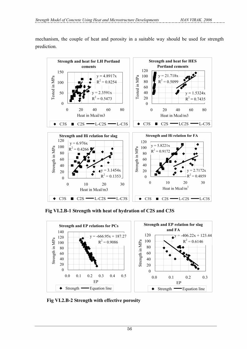
Strength Model of Concrete Using Heat and Microstructure Developments HAN VIRAK. 2006
56
mechanism, the couple of heat and porosity in a suitable way should be used for strength prediction.
Strength and heat for LH Portlandcements
y = 4.8917xR2 = 0.8254
y = 2.3591xR2 = 0.5473
0
50
100
150
0 20 40 60 80Heat in Mcal/m3
Test
ed in
MPa
C3S C2S L-C2S L-C3S
Strength and heat for HESPortland cements
y = 21.718xR2 = 0.5099
y = 1.5324xR2 = 0.7435
020406080
100120
0 20 40 60 80Heat in Mcal/m3
Test
ed in
MPa
C3S C2S LC2S L-C3S
Strength and Hi relation for slag
y = 6.976xR2 = 0.4266
y = 3.1454xR2 = 0.13530
20406080
100120
0 10 20 30Heat in Mcal/m3
Stre
ngth
in M
Pa
C3S C2S L-C2S L-C3S
Strength and Hi relation for FA
y = 5.8221xR2 = 0.9172
y = 2.7172xR2 = 0.48590
20406080
100120
0 10 20 30Heat in Mcal/m3
Stre
ngth
in M
Pa
C3S C2S L-C2S L-C3S
Fig VI.2.B-1 Strength with heat of hydration of C2S and C3S
Strength and EP relations for PCs
y = -666.95x + 187.27R2 = 0.9086
020406080
100120140
0.0 0.1 0.2 0.3 0.4 0.5EP
Stre
ngth
in M
Pa
Strength Equation line
Strength and EP relation for slagand FA
y = -406.22x + 123.44R2 = 0.6146
020406080
100120
0.0 0.1 0.2 0.3EP
Stre
ngth
in M
Pa
Strength Equation line
Fig VI.2.B-2 Strength with effective porosity

Strength Model of Concrete Using Heat and Microstructure Developments HAN VIRAK. 2006
57
The strength prediction should generally bear the form given as follows:
),( ic HPgf = ..........................................................................................................eq. 61
where cf is the strength of concrete, mortar or paste.
P, Hi are respectively porosity of mix and unit total heat of each compound. ),( iHPg is a function in which porosity and heat are coupled together.
The function ),( iHPg can be proposed in the following forms:
∑=
=compoundsAll
ndeachcompoui
iii P
HaHPg ),( ...................................................................................eq. 62
or
∑=
−=
compoundsAll
ndeachcompouiiii H
PIPPIaHPg .),( ........................................................................eq. 63
In these forms, P represents one pore type or a combination of pore type. It can be gel pore, capillary pore, effective pore, total pore or other combination. The following study will show which type of pore should be used for strength prediction.
VI.3. Proposed model
VI.3.A. Strength function with P
Hi
The study will be based on the relation between strength with Hi and P which can be in three cases (effective pore, capillary pore and total pore). Fig.VIII.2.-1 shows, for the case of low heat Portland cement, the linearity between strength fc with heat of each component divided by the following pore types:
• Effective porosity (EP): EPH i
• Total porosity (TP): TPHi and
• Capillary porosity (CP): CPH i .
As can be shown, fc has a better linearity with Hi/EP than with Hi/TP and much better than with Hi/CP.

Strength Model of Concrete Using Heat and Microstructure Developments HAN VIRAK. 2006
58
In addition, Fig.VIII.2-2 shows, for the case of high early strength Portland cement mortar, the linearity of strength fc with Hi/EP, Hi/TP and Hi/CP. As can be seen, fc with Hi/CP can not be related with linear function however strength gives a linear relation a little better for Hi/TP than for Hi/EP. LH and HES cements are two cements which contain the extreme amount of C2S and C3S for Portland cements. So from this viewpoint, the conclusion is that linearity of strength with Hi/EP and Hi/TP is better than with Hi/CP for the case of all Portland cements.
The same study is conducted for the case of slag and fly ash replacement. Fig.VIII.2-3 and VIII.2-4 show the relation between strength and Hi/EP and Hi/TP. All points (strength and Hi/P) are scattered but the relation of strength with Hi/EP gives smaller scatter than with Hi/TP. So the parameter that should be used in strength prediction model is probably Hi/EP.
In general, it is found that the regression coefficient is higher than 0.75 for all Portland cements when strength is related to Hi/EP by a linear function. The scatter seems high however this scatter is not the strength prediction problem as the strength model is going to be a sum of contribution of all compounds multiplied with Hi/EP so that the scatter would be changed and that the smaller scatter of the relation between fc and Hi/P the smaller the strength prediction scatter. So we are going now to establish the model and check if the scatter for strength prediction is acceptable. Finally the following expressions can be approximately written:
EPH
af iic = ...............................................................................................................eq. 64
In order to predict as function of compound composition, fc needs to be related to all compounds, the relation becomes:
( )∑ +++==i
AFCAFCACACSCSCSCSCi
ic HaHaHaHaEPEP
Haf 44333322
1 ...............eq. 65
AFCACSCSC aandaaa 4332 ,, are to be determined from the experimental data. Using the strength tested on Portland cement mortars, these coefficients are 0.33, 0.17, -0.032 and 0.43. So the equation eq.65 becomes:
( )AFCACSCSCc HHHHEP
f 4332 43.0032.017.033.01+−+= ..................................eq. 66
Eq.66 expresses that the contributions of all compounds are positive except that of C3A which is negative. According to Bogue, all contributions are individually positive however the contribution of C3A in the model is negative. This is because when all compounds are mixed

Strength Model of Concrete Using Heat and Microstructure Developments HAN VIRAK. 2006
59
their contributions are interacted to each other so that their contributions are different from the individual contribution. The compound C3A, which produces ettringite and monosulfate accompanying an expansion, may be a source of strength reduction as can be indicated by the equation its contribution is -0.032. Blaine R. L. (1968) and Von Euw M. (1970) et al. reported that C3A has a positive influence effect up to 7 or 28 days but negative influence later on.
Prediction for low heat cement
y = 0.9892xR2 = 0.9597
1030507090
110130
0 20 40 60 80 100 120Modeled strength in MPa
Test
ed st
reng
th in
MPa
.
Prediction regression line
Prediction for OPC cement
y = 0.9809xR2 = 0.8206
20406080
100120140
20 40 60 80 100 120 140
Modeled strength in MPaTe
sted
stre
ngth
in M
Pa.
Prediction regression line
Prediction for HES cement
y = 0.9944xR2 = 0.8192
20406080
100120140
20 40 60 80 100 120 140
Modeled strength in MPa
Test
ed st
reng
th in
MPa
.
Prediction regression line
All Portland Cement Prediction
y = 0.9884xR2 = 0.8995
20406080
100120140
20 40 60 80 100 120 140Modeled in MPa
Test
ed in
MPa
Predictions LPC
Fig VI.3.A-1: Strength Prediction by eq.66
Fig.VI.3.A-1 shows the prediction precision of each type of cement by eq.66. For LH cement, the prediction is very good with a regression coefficient of 0.96 however this regression decreases for OPC and HES cements. The reason may be the rapid hydration of OPC and HES cement which can modify the pore microstructure. Verbeck and Helmuth suggested that rapid hydration led to encapsulation of the cement grains by a product of low porosity which retarded or prevented further hydration. Another reason may be the change of fracture mechanism when strength is high.

Strength Model of Concrete Using Heat and Microstructure Developments HAN VIRAK. 2006
60
The relation between strength and ( ) bai PH / was also studied for the case of C2S and C3S
but the variations of a and b will just make the regression coefficients of a compound increase and another decrease. The same linearity for C2S and C3S is obtained with a=1 and b=1.
VI.3.B. Strength function with iHPI
PPI .−
In the previous section, the term 1/EP is the factor of sum of heat of compounds in powder. The problem that poses in the previous case is that when EP becomes very small or zero the strength predicted will be infinite. In an attempt that strength would be zero when P equals an initial value or one constant when P becomes zero, the strength expression should be the following:
∑−=
all
iiic Ha
PIPPIf ................................................................................................eq. 67
where
• PI is the initial porosity
• P is a current porosity and
• Other symbols are the same as in the previous section.
We are going to study which porosity should be determinant for strength prediction when eq.67 is used. PI is the porosity just before the hydration is started, so PI is equal to volume of water. Then eq.67 becomes:
∑=
−=
compoundsall
compoundeachiii
W
Wc Ha
VPV
f . ........................................................................................eq. 68
In this study, all portland cements including LH, OPC and HES are used. The w/c ranges from 0.3 to 0.6 with curing conditions alternatively wet and sealed. Fig.VIII.3-1 shows the relationship between strength and Hi*(Vw-P)/Vw for LH cement. It is found that strength is linear to Hi*(Vw-EP)/Vw, Hi*(Vw-TP)/Vw and Hi*(Vw-CP)/Vw with the same regression coefficient only the slopes of regression line are different. This may explains that either of these three parameters can be used in strength prediction modeling for LH cements. The same conclusion is found for HES cements as can be shown in Fig.VIII.3-2. However in case of slag replacement, only Hi*(Vw-EP)/Vw is a good linear relation with strength as can be seen

Strength Model of Concrete Using Heat and Microstructure Developments HAN VIRAK. 2006
61
in Fig.VIII.3-3. Contrary to the case of slag replacement, for fly ash replacement, strength is found having a good linear relation with all of three parameters described above. In conclusion, the parameter H*(Vw-EP)/Vw should be used in strength modeling because it can provide better linearity with strength than other parameters. The equation becomes:
∑=
−=
compoundsall
compoundeachiii
W
Wc Ha
VEPV
f . .....................................................................................eq. 69
Using the experimental data, eq.69 becomes:
( )AFCACSCSCW
Wc HHHH
VEPV
f 4332 1116.08.12. +−+−
= ......................................eq. 70
Portland Cement Model Prediction
y = 1.0094xR2 = 0.9317
10
30
50
70
90
110
130
10 30 50 70 90 110 130Modeled in MPa
Test
ed in
MPa
Predictions LPC
Fig VI.3.B-1: Strength prediction for all mortar made with Portland cements (eq.70)
The fig.VI.3.B-1 shows the strength tested and strength modeled with eq.70. As can be seen, the scatter of strength predicted starts when the strength of mortar is higher than 70-80 MPa and When strength is higher than 100MPa, the modeled strength has tendency to be lower than the tested strength. The reason may be the fracture mechanism which changes when strength is high.
When strength is low, it has been known that the fracture started from aggregate-paste interfaces and spread into the paste and adjacent interfaces until final rupture however when strength is high, fracture originated in the interfaces and spread by breaking the aggregate. As the fracture mechanism changes, the strength is not only affected by the cement paste but also by the surface texture and the mechanical strength of aggregate used which are not considered as the parameters in this research. These parameters should be studied more in future.
Comparing the model given by eq.66 and the one given by eq.70, it is found that eq.70 provides better prediction than eq.66 and that eq.70 gives the finite prediction in all cases however eq.66 gives the infinite value when porosity become too small or zero. So the model by eq.70 should be proposed for strength prediction. In next sections, we are going to treat the

Strength Model of Concrete Using Heat and Microstructure Developments HAN VIRAK. 2006
62
cases of powder replacement with eq.70.
VI.3.C. Contribution of compounds with age
It was reported that pure compounds of C2S, C3S, C3A and C4AF have strength positive as can be shown in fig VI.6-1 by Bogue (1955), however the compounds have interaction effect between themselves so that the contribution of each compound under interaction can be negative as can be shown by the model equation. One question have been posed was whether the contributive coefficient of compounds change with age. The calculation is made to find contributive coefficients for each compound with age. When a cement grain is reacted with water, reaction starts at the surface and then grows inwards at the same time that the particle expands outwards as can be illustrated in fig VI.3.C-1. This means that at an age of curing, old hydrates and young hydrates exist together.
Fig VI.3.C-1 Reacting grain of cement
The contributive coefficients are calculated and shown in Table VI.3.C-1. The change behaviors of contributions are illustrated in Fig VI.3.C-2. As can be seen, for C3A the contribution is positive for early ages and negative for longer ages however C2S and C3S have negative contributions for early ages and positive ones for longer ages.
Table VI.3.C-1 Contributive coefficients of compounds as a function of age
Age C3A C4Af C2S C3S 7 6.5 55.8 -32.0 -1.9 14 1.2 22.7 -6.1 1.0 28 -0.08 13.5 0.6 1.73 91 -0.16 11.2 2.1 1.8
Age
Expansion Younger
Unhydrated+ WATER = Oldly hydrated
Newly hydrated
Cement Expanding hydrates

Strength Model of Concrete Using Heat and Microstructure Developments HAN VIRAK. 2006
63
The reason why C3A has contribution which changes from positive to negative may be due to the hydrate fracture mechanism determining strength participation of compounds. As hydration progresses, hydrated structures are composed of Portlandite (CH) and calcium silicate hydrate of different types (CSH) with the presence of small amount of AFt and AFm.
Contribution of C3A
-101234567
0 20 40 60 80 100Age in day
Con
tribu
tion
coef
icie
nt .
C3A
Contribution of C4AF
0102030405060
0 14 28 42 56 70 84Age in day
Con
tribu
tion
coef
icie
nt .
C4AF
Contribution of C2S
-32
-24
-16
-8
0
8
0 14 28 42 56 70 84Age in day
Con
tribu
tion
coef
icie
nt .
C2S
Contribution of C3S
-2
-1
0
1
2
0 14 28 42 56 70 84Age in day
Con
tribu
tion
coef
icie
nt.
C3S
Fig VI.3.C-2 Change of strength contributions
According to fractographic studies of Dalgleish, B. J. about hydrated Portland cement, it was reported that in young pastes interparticle fracture occurs through the developing gel and around the rigid inclusions of CH with some AFt and AFm. As cement paste matures, CH crystals form a massive structure so that an interparticle crack path becomes too tortuous and the energy requirement exceeds that for CH cleavage. Alternatively, CSH becomes denser and develops strength so much that the fracturing energy becomes similar to that of CH cleavage. The failure in mature pastes occurs via a relatively straight path through extensive region of CH and dense massive CSH at the same time that AFt and AFm grows in isolated porosities. This suggests that for young paste, strength is strongly played by CH and AFt and AFm however the strength change to be played by CH and CSH when the paste ages. The growth of AFt and AFm in isolated porosities expresses the negative contribution of C3A. In addition

Strength Model of Concrete Using Heat and Microstructure Developments HAN VIRAK. 2006
64
to Dalgleish's report, Blaine R. L. (1968) and Von Euw M. (1970) et al. reported that C3A has a positive influence effect up to 7 or 28 days but negative influence later on. So the change of strength contribution as function of time agrees with other researchers' findings.
VI.4. Model with slag and fly ash replacement
When slag or fly ash is used, these materials can react with catalysts produced by cement and produce the similar hydration products (CSH) as pure cement paste and take part in strength the only difference between slag or fly ash paste from the pure cement paste is the content of Ca(OH)2 which high in cement paste. So slag and fly ash are also sources contributing to strength. In order to include slag and fly ash in the model, the contributions of slag and fly ash have to be determined. In case of slag, it was reported that the replacement ratio can reach 80% but in general, the maximum replacement ratio is reported 60% for low w/p. Two slag replacement ratios are used: 20% and 60% for w/p=0.3 however for w/p=0.45 and 0.6, only the slag replacement ratio equal to 20% is used. On the other hand, in case of Fly ash, the replacement ratio is 20% for w/p=0.3, 0.45 and 0.6. Using experimental data (see table.VIII.1-6, VIII.1-9 and VIII.1-11), their contributions are found and the model becomes:
)4.149.0
1116.08.12.( 4332
FASG
AFCACSCSCW
Wc
HH
HHHHV
EPVf
++
+−+−
=......................................eq. 71
Slag and flyash Model Prediction
y = 0.9957xR2 = 0.9391
1030507090
110130
10 30 50 70 90 110 130Modeled in MPa
Test
ed in
MPa
Predictions EQL
Fig VI.4-1: Strength prediction for slag and fly ash replacement case
Fig.VI.4-1 shows how much the tested strengths are different from the modeled ones in case of mixes with slag and fly ash replacements. The strength can be well predicted by the model eq.71. Comparing with the fig.VI.3.B-1, one observation is that for slag and FA mixes, even strength is high but the strength still can be predicted without fracture type effects.
VI.5. Model for mixes with LS
Limestone is not totally reactive but its physical and chemical properties allow this powder to

Strength Model of Concrete Using Heat and Microstructure Developments HAN VIRAK. 2006
65
affect the compressive strength. Physically, limestone plays a function as filler between the clinker grains. At the same time, the additional surface area provided by the limestone particles may provide sites for the nucleation and growth of hydration products, generally enhancing the achieved hydration. Both the increase of hydrates and the presence of LS as filler are contributive to strength. Chemically, when LS is used the presence of monosulfate is not observed because LS reacts with monosulfate to give mono-carboaluminate (CaO)3(Al2O3).CaCO3.11H2O and mono-sulfoaluminate (CaO)3.(Al2O3).CaSO4.12H2O. The reaction takes place to an extent depending on the dosage of LS itself. The phenomena in which the hydration products are modified when LS is used can affect strength to some extent. The question is how the two properties of LS can affect the strength model. Answering to this question, the prediction of strength of LS mixes with the proposed model should be studied. Using eq.70, the prediction for limestone replacement is shown in the following figure.
Prediction for LS
y = 1.4042xR2 = 0.9514
102030405060708090
10 20 30 40 50 60 70 80 90
Modeled strength in Mpa
Test
ed s
treng
th in
Mpa
.
Prediction regression line
fc = (Vw-EP)/Vw*(2 HC2S +1.8 HC3S- 0.16 HC3A+11 HC4AF)
In fig.VI.5-1, the strength predicted by the model is lower than the ones tested. Even the heat model takes already in account the effect, the LS effect on strength has to be regarded. The strength of the LS mixes depends of course on the strength of four compounds of cement and also on the LS effect in filling the porosity of paste and increasing the strength. This LS effect is found 1.4 as shown with the slope of prediction line.
Fig VI.5-1: Strength Prediction for LS without effect of LS
As can be seen in Fig.VI.5-1, the strength is 1.4 times higher than the predicted strength. This is to say that the LS effect is 1.4. The LS replacement is PLS = 20% so the LS effect (LSE) can be written as
LSE = 1 + 0.02 PLS.................................................................................................eq. 72
The equation becomes then
( ) )02.01(*1116.08.12. 4332 PLSHHHHV
EPVf AFCACSCSC
W
Wc ++−+
−= .............eq. 73
LSE is a coefficient which increases the contributions of compounds (C3S, C2S, C3A and C4AF) in cement. One question is whether LSE can be introduced as a heat rate accelerator

Strength Model of Concrete Using Heat and Microstructure Developments HAN VIRAK. 2006
66
into the multi-component heat model. Of course, LS can affect the heat of hydration but LSE coefficient expresses only the increase of strength contributions when LS is used. This can not express that heat can be increased by multiplying with LSE. The heat was not measured in the experiment however was just calculated with the model. There may be a need to make an investigation by measuring heat to see whether LSE can be integrated into the multi-component heat model.
Prediction for LS with LS effect
y = 1.003xR2 = 0.9514
102030405060708090
100
10 20 30 40 50 60 70 80 90 100
Modeled strength in MPa
Test
ed st
reng
th in
MPa
.
Prediction regression line
fc = (Vw-EP)/Vw*(2 HC2S+1.8 HC3S - 0.16 HC3A+11 HC5AF)*(1+0.02 PLS)
As can be seen in Fig.VI.5-2, the introduction of LS effect (LSE) in the model allows a good prediction. When the LS replacement is zero, the LSE becomes 1. The LS effect is determined by supposing that the effect is linear with the LS percentage. The proposed model can predict strength with LS for different w/c.
Fig VI.5-2: Strength Prediction for LS with effect of LS
According to the above illustrations concerning strength in function of heat and porosity for all cases including Portland cements, slag, flyash and limestone powder replacement, it was found that strength has a linear function with heat coupled with effective porosity.
VI.6. Two-compound modeling
According to Bogue (1955), each compound has its own strength as can be presented in Fig VI.6-1. The strengths of C3S and C2S are approximately the same for long time and are higher than strength of C3A and C4AF. The fact that strength of C3A and C4AF are very small can give an idea to neglect the contribution of these two compounds. In this section, an attempt is made to find a model of strength basing on two compounds including C2S and C3S.

Strength Model of Concrete Using Heat and Microstructure Developments HAN VIRAK. 2006
67
Fig VI.6-1 Strength of pure compounds (Bogue, 1955)
VI.6.A. Two-compound model for Portland cements
When only two compounds C2S and C3S are taken into account, the equation becomes:
( )SCSCW
Wc HH
VEPV
f 32 6.26.6. +−
= ........................................................................eq. 74
Portland Cement Strength Model Prediction
y = 0.9888xR2 = 0.9137
1030507090
110130
10 30 50 70 90 110 130Modeled
Test
ed
Predictions LPC
As can be shown in Fig VI.6.A-1, the strength can be predicted with two compounds for all Portland cements.
Fig VI.6.A-1 Prediction for Portland cements by two-compound model

Strength Model of Concrete Using Heat and Microstructure Developments HAN VIRAK. 2006
68
VI.6.B. Two-compound model for Powder replacement The model proposed with eq.74 is extended for cases of slag, fly ash and limestone replacement. The following equation:
[ ]FASGSCSCW
Wc HHPLSHH
VEPV
f 4.149.0)02.01(*)6.26.6. 32 ++++−
= .............eq. 75
Blended powder+ PC Model Prediction
y = 0.9991xR2 = 0.9386
10
30
50
70
90
110
130
10 30 50 70 90 110 130Modeled
Test
ed
Predictions EQL
Fig VI.6.B-1 Prediction for powder replacement mixes by two compounds
VI.7. Prediction for other sources of data
The preceding section has shown that the model can predict well the strength of mortar that have the ideal conditions as in microstructure and multi-component heat models. Now the prediction for other sources of data is going to be presented in this section. The data from UBE-Mitsubishi cement corporation contains standard mortars, normal strength concrete and high strength concrete using Portland cements including LH (low heat cement), OPC (ordinary Portland cement) MH (Medium heat cement) and HES (high early strength). In addition, the data from Sumitomo Osaka cement (Meca cements) contains standard mortars using 5 different LH cements and HES.
With the sources of data from Sumitomo Osaka and UBE-Mitsubishi, some main differences are:
• Dispersion which is probably much different. • Volume of aggregate • Aggregate type

Strength Model of Concrete Using Heat and Microstructure Developments HAN VIRAK. 2006
69
Table VI.7-1 shows quantitatively and qualitatively some differences between the data obtained by the authors' experimental works and the data from the external sources (Sumitomo Osaka and UBE-Mitsubishi cement Corporation).
Table VI.7-1: Main differences of other sources of data Own data External sources Dispersion Maximum dispersion Unknown dispersion
Aggregate volume (m3) • 0.37 (w/c=0.3) • 0.47 (w/c=0.45) • 0.52 (w/c=0.6)
• 0.567 (Standard mortar) • 0.7-0.71 (Normal concrete) • 0.63-0.67 (High strength
concrete) Aggregate type Mountainous Unknown Sand Specific gravity 2.59 2.63
Meca and UBE standard mortarstrength
y = 1.3148xR2 = 0.8901
01530456075
0 50Modeled in MPa
Test
ed in
MPa
Test Prediction slope
UBE-High Strength Concrete
y = 1.4627xR2 = 0.8584
020406080
100
0 20 40 60 80 100Modeled in MPa
Test
ed in
MPa
UBE Prediction slope
Normal concrete (UBE)
y = 1.4988xR2 = 0.8448
0
20
40
60
80
0 10 20 30 40 50 60 70
Modeled in MPa
Test
ed in
MPa
Normal Concrete Prediction slope
It is found that strength predicted for standard mortars and for normal and high strength concrete are linear with modeled strength. The slope of prediction is 1.3 for mortars and 1.46 for high strength concrete and 1.50 for normal concrete. This means that the predictions are lower than test results.
Fig VI.7-1: Strength Prediction for different data sources
Fig.VI.7-1 shows the strength of mortars and concrete predicted using the proposed model.

Strength Model of Concrete Using Heat and Microstructure Developments HAN VIRAK. 2006
70
The prediction indicates different slopes for different cases but the particularity is that all tested strength points are related to modeled ones by a line. This means that strength is linear to the couple of heat and effective porosity.
The reason why the prediction gives low values is that data from UBE and Sumitomo might be produced using different sand (see table VI.7-1). In addition, sand type and aggregate effects become the new factor that more research should be conducted.
VI.8. Applicability of model
The model was established to predict strength of Portland cements and some powder replacement such as slag, fly ash and limestone. The calculation tool is microstructure and multi-component heat development models which are applicable particularly only to Portland cements and blended powders.
The Portland cements are very often used due to their properties compatible with many purposes of civil engineering however CACs (Calcium Aluminate Cements) are also used in construction for some special treatment due to their properties including rapid strength development, good resistance to sulfate and many other forms of chemical attack and are good for making refractory concrete.
CACs have the composition quite different from those of Portland cements. CACs contain high amount of Al2O3 and very low amount of SiO2 however Portland cements contain low amount of Al2O3 and high amount of SiO2. Due to the difference of compositions, the hydration products are quite different:
Table VI.8-1: Portland cements and CACs
Portland cements CACs
Hydration Products CSH, CH CAH10, C2AH8, C3AH6, AH3
Multi-component heat model Applicable Not applicable
TableVI.8-1 shows some data that can explain that strength of Portland cements and CACs are affected with contributions made by other different compounds. In addition, the multi-component heat model can calculate only the heats of hydration of Portland cements. So this proposed model is applicable only to Portland cements.
Strength Model of Concrete Using Heat and Microstructure Developments HAN VIRAK. 2006
71
CHAPTER VII: CONCLUSIONS VII. Conclusions
VII.1. General conclusions
After a long and careful discussion based on the experimental data from different sources and with other researchers' findings, a model was successfully proposed. On the strategic way, the authors' experimental data showed some interesting findings among which some were confirmed by other researchers and some others were originally new. The whole research could be concluded in the following summary.
1. In common sense, strength of cementitious materials was essentially dependent of w/p. In this research, some more subsidiary parameters that could make the strength vary remarkably were presented and their effects on strength were clarified. The sand content showed its effect on strength by the existence of aggregate critical volume higher than which strength varied increasingly or decreasingly depending on the dispersion level. The critical volume was found 0.37 for w/c=0.3 and 0.52 for w/c=0.6. The lower w/c, the lower critical volume.
2. The super-plasticizer was found affecting strength with a non-negligible increase when it was increased higher than the amount of SP absorbed by the surface of powder. The absorbed SP was found 0.3% that was not effective in dispersing and the dispersion increased until SP dosage=1.0% where the strength was maximum for different w/c. The effect of SP was higher when the w/c was lower.
3. The mixing time was found playing a smaller influence on strength than the sand content and the SP dosage. The mixing time 3 min was found optimum for obtaining the maximum strength and with higher mixing times, strength was kept constant for low w/p however strength was decreased for high w/p. This was explained with the fact that the false and real w/p were different at high w/p. With different mixing times, the strength was optimum using SP=1.0%.
4. LS powder has become a material currently used to replace cement for effective cost savings without long-term deterioration. To obtain the maximum strength, the SP dosage (without LS) was found different when LS was used. By using the strength data, the

Strength Model of Concrete Using Heat and Microstructure Developments HAN VIRAK. 2006
72
discussion concluded that LS could absorb some SP and the dosage had to be increased in order to acquire the maximum strength or high dispersion. The strength of mix without LS at SP=0 was found comparable to the strength with 20% LS replacement at SP/P=1.18%.
5. Using the mixes of ideal conditions as described in the microstructure and multi-component heat models, it was clearly found that strength had a linear relation with the couple of heat of hydration with effective porosity of each compound. Strength can then be a summation of all heat-pore components.
6. The proposed model:
After the contribution coefficients of all compounds were determined, the model was proposed with:
)4.149.0
).02.01(*)1116.08.12(.( 4332
FASG
AFCACSCSCW
Wc
HH
PLSHHHHV
EPVf
++
++−+−
=
This was applicable to mixes made with Portland cements and powders including limestone powder, fly ash and slag for different w/c and different curing conditions.
7. If the model is simplified with the two compounds C2S and C3S, the model becomes:
)4.149.0).02.01(*)6.26.6(.( 32 FASGSCSCW
Wc HHPLSHH
VEPV
f ++++−
=
8. Using the data from different sources, the prediction still shows that the strength had a linear relation with hydration heat and effective porosity in all cases. Owing to some intervention of further parameters listed in table VI.7-1, the current model needed to be refined considering more parameters.
VII.2. Model improvement
Even with data provided by other sources, charts of tested strength-modeled strength explain that tested strength has relation linear with the modeled strength which is linear to the couple of heat and porosity. The tested-modeled line shows some slope expressing the intervention of some further effects. The model was created with the experimental data in which the dispersion was maximum (dispersion), mixes were free of sand content effect (aggregate volume), sand was the mountainous one (type of aggregate). So when the aggregate of different types, different contents are used, the effect of aggregate content and the effect of

Strength Model of Concrete Using Heat and Microstructure Developments HAN VIRAK. 2006
73
aggregate type play their roles in strength. In addition, when the SP of different types and different dosages are used, the dispersion effect becomes another factor affecting the strength. In order to improve the proposed model for wide application, the following should be included in the model:
1. Dispersion effect
• SP type: there are mainly 4 types of super-plasticizers which have different delaying effects due to its structure and its manner of adhering to cement particles.
• SP dosage: this parameter exercises a direct effect on strength. It was shown that there exist non-effective SP and effective SP which may vary with the type of SP.
2. Aggregate effect
• Aggregate type: different types of aggregate have different surface texture which affects the aggregate-paste bonding effect.
• Aggregate content: aggregate can interact and play an effect on strength when its content is higher than the critical volume.
• Aggregate size: aggregate is one source of local bleeding which is the weak part of concrete. The larger the size is, the more localized the weakness is. This is a source affecting strength.
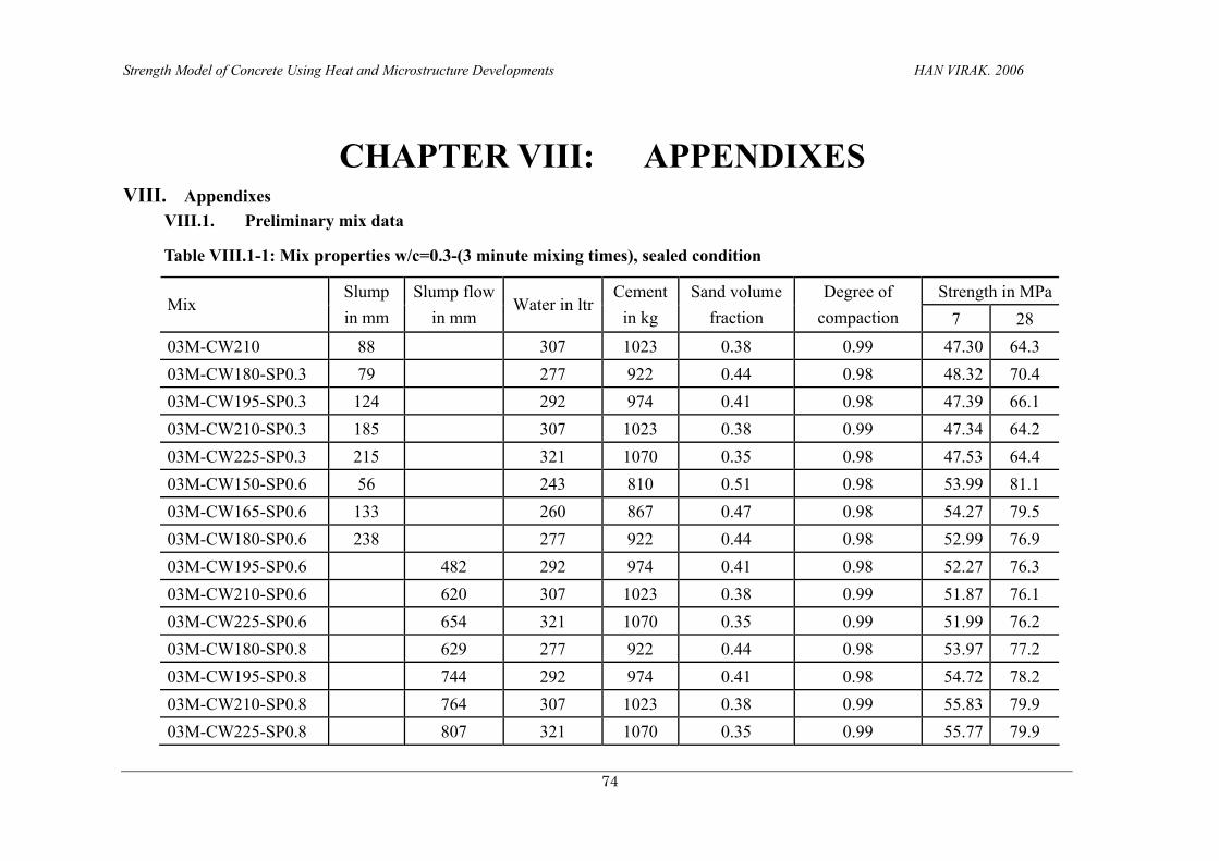
Strength Model of Concrete Using Heat and Microstructure Developments HAN VIRAK. 2006
74
CHAPTER VIII: APPENDIXES VIII. Appendixes
VIII.1. Preliminary mix data
Table VIII.1-1: Mix properties w/c=0.3-(3 minute mixing times), sealed condition
Strength in MPaMix
Slump in mm
Slump flow in mm
Water in ltrCement
in kg Sand volume
fraction Degree of
compaction 7 28 03M-CW210 88 307 1023 0.38 0.99 47.30 64.3 03M-CW180-SP0.3 79 277 922 0.44 0.98 48.32 70.4 03M-CW195-SP0.3 124 292 974 0.41 0.98 47.39 66.1 03M-CW210-SP0.3 185 307 1023 0.38 0.99 47.34 64.2 03M-CW225-SP0.3 215 321 1070 0.35 0.98 47.53 64.4 03M-CW150-SP0.6 56 243 810 0.51 0.98 53.99 81.1 03M-CW165-SP0.6 133 260 867 0.47 0.98 54.27 79.5 03M-CW180-SP0.6 238 277 922 0.44 0.98 52.99 76.9 03M-CW195-SP0.6 482 292 974 0.41 0.98 52.27 76.3 03M-CW210-SP0.6 620 307 1023 0.38 0.99 51.87 76.1 03M-CW225-SP0.6 654 321 1070 0.35 0.99 51.99 76.2 03M-CW180-SP0.8 629 277 922 0.44 0.98 53.97 77.2 03M-CW195-SP0.8 744 292 974 0.41 0.98 54.72 78.2 03M-CW210-SP0.8 764 307 1023 0.38 0.99 55.83 79.9 03M-CW225-SP0.8 807 321 1070 0.35 0.99 55.77 79.9

Strength Model of Concrete Using Heat and Microstructure Developments HAN VIRAK. 2006
75
03M-CW210-SP1.0 889 307 1023 0.38 0.99 56.83 81.2 03M-CW210-SP1.2 - 307 1023 0.38 1.00 56.03 81.5
Table VIII.1-2: Mix properties w/c=0.6-(3 minute mixing times), sealed condition
Strength in MPaMix
Slump in mm
Slump flow in mm
Water in ltr
Cement in kg
Sand volume fraction
Degree of compaction 7 28
06M-CW195 564 318 531 0.52 1.00 11.52 31.3006M-CW150-SP0.2 110 261 435 0.61 0.99 10.46 31.5706M-CW165-SP0.2 230 281 468 0.57 0.99 12.06 31.4106M-CW180-SP0.2 541 300 500 0.55 1.00 11.60 30.7306M-CW195-SP0.2 630 318 531 0.52 1.00 11.25 30.6706M-CW210-SP0.2 784 336 560 0.49 1.01 11.18 30.8606M-CW195-SP0.4 670 318 531 0.52 1.00 11.69 33.6206M-CW195-SP0.6 768 318 531 0.52 0.99 12.83 34.8406M-CW150-SP0.8 240 261 435 0.61 0.99 10.84 32.4106M-CW165-SP0.8 577 281 468 0.57 0.99 11.47 34.3306M-CW180-SP0.8 788 300 500 0.55 1.00 12.85 36.1106M-CW195-SP0.8 871 318 531 0.52 1.00 15.18 39.3806M-CW210-SP0.8 - 336 560 0.49 1.00 15.33 39.9906M-CW195-SP1.0 - 318 531 0.52 1.01 16.43 42.2906M-CW195-SP1.2 - 318 531 0.52 1.01 14.82 35.21

Strength Model of Concrete Using Heat and Microstructure Developments HAN VIRAK. 2006
76
Table VIII.1-3: Mix properties w/c=0.3, seal condition
Strength in MPaMix
Slump flow in mm
Degree of compaction 7th day 28th day
03M-CW210SP0.8-2mn 798 0.99 52.55 74.6103M-CW210SP1.0-2mn - 0.99 54.06 77.9903M-CW210SP1.2-2mn - 0.99 54.02 78.8903M-CW210SP0.8-5mn 810 0.99 55.83 79.5503M-CW210SP1.0-5mn - 0.99 56.82 81.3603M-CW210SP1.2-5mn - 0.99 56.71 82.0703M-CW210SP0.8-10mn 765 0.97 54.91 78.3403M-CW210SP1.0-10mn - 0.98 56.95 81.9703M-CW210SP1.2-10mn - 0.99 56.74 82.47
Table VIII.1-4: Mix properties w/c=0.6, seal condition
Strength in MPaMix
Slump flow in mm
Real w/cDegree of
compaction 7th day 28th day06M-CW195SP0.8-2mn 893 0.55 1.00 14.93 38.7106M-CW195SP1.0-2mn - 0.55 1.00 16.55 40.5306M-CW195SP1.2-2mn - 0.55 1.01 15.33 36.1206M-CW195SP0.8-5mn - 0.58 1.00 13.85 36.2106M-CW195SP1.0-5mn - 0.57 1.00 14.67 37.2306M-CW195SP0.8-10mn - 0.59 1.00 12.47 34.4806M-CW195SP1.0-10mn - 0.59 1.00 13.44 36.28

Strength Model of Concrete Using Heat and Microstructure Developments HAN VIRAK. 2006
77
Table VIII.1-5: Mix proportion of mortars using low heat, OPC and high early strength cements
Mix name w/p water Flow (small cone) in mm
PowderSand SSD
Sand volume
LH 03M-CW210SP1.0 0.3 307 300 1023 970 0.38 045M-CW202SP1.0 0.45 326 303 724 1159 0.45 06M-CW195SP1.0 0.6 318 290 531 1331 0.51 OPC 03MCW210SP1.0 0.3 306 250 1018 964 0.37 045M-CW202SP1.0 0.45 325 300 722 1158 0.45 06M-CW195SP1.0 0.6 318 243 529 1333 0.52 HES 03M-CW210SP1.0 0.3 305 180 1017 956 0.37 045M-CW202SP1.0 0.45 316 242 701 1192 0.46 06M-CW195SP1.0 0.6 317 240 529 1330 0.51

Strength Model of Concrete Using Heat and Microstructure Developments HAN VIRAK. 2006
78
Table VIII.1-6: Mix proportions with powders
Mix name w/p WaterFlow (small cone) in mm
Powder kg
Sand SSD in kg
Cement LH %
Powder replacement
ratio %
Sand volume
Limestone replacement 045M-CW202LS20 0.45 315 328 701 1190 80 20 0.46 06M-CW195LS20 0.6 317 305 529 1329 80 20 0.51 03M-CW210LS20 0.3 305 350 1016 949 80 20 0.37 Fly ash replacement 03M-CW210FA20 0.3 303 290 1010 938 80 20 0.36 045M-CW202FA20 0.45 314 300 699 1177 80 20 0.45 06M-CW195FA20 0.6 316 280 527 1318 80 20 0.51 Slag replacement 03M-CW210SL20 0.3 306 380 1019 965 80 20 0.37 03M-CW210SL60 0.3 303 350 1011 941 40 60 0.36 045M-CW202SL20 0.45 316 330 702 1197 80 20 0.46 06M-CW195SL20 0.6 318 360 530 1334 80 20 0.52

Strength Model of Concrete Using Heat and Microstructure Developments HAN VIRAK. 2006
79
Table VIII.1-7: Test results of mixes with limestone replacement
SP ratio in weight Strength (MPa) SP ratio in volume SP/P SP/C
Flow (small cone) in mm
D-ratio7 14 28 91 SP/C SP/P
0.70% 0.88% 220 0.97 43.85 - 74.66 - 5.2% 4.0% 0.86% 1.08% 250 0.97 44.47 - 75.62 - 2.7% 2.1% 1.02% 1.28% 300 0.98 46.49 - 80.40 - 3.3% 2.6% 1.18% 1.48% 350 0.99 51.35 - 84.35 - 4.6% 3.5%
03M-CW210LS20
1.34% 1.68% 405 1.00 49.35 - 82.09 - 5.2% 4.0% 0.86% 1.08% 301 1.00 20.37 - 44.81 - 3.3% 2.6% 1.02% 1.28% 328 1.00 20.67 33.15 45.73 69.24 40% 3.1%
045M-CW202LS20
1.18% 1.48% 380 1.00 20.64 - 46.05 - 4.6% 3.5% 1.02% 1.28% 267 1.00 9.67 - 24.24 - 4.0% 3.1% 1.18% 1.48% 305 1.00 12.06 16.24 26.26 42.78 4.6% 3.5%
06M-CW195LS20
1.34% 1.68% 333 1.00 11.89 - 26.65 - 5.2% 4.0%

Strength Model of Concrete Using Heat and Microstructure Developments HAN VIRAK. 2006
80
Table VIII.1-8: Dosage of SP for mixes with fly ash replacement
Dosage in weight Dosage in volume SP/P SP/C SP/P SP/C 045M-CW202FA20-wet 1.02% 1.28% 3.06% 3.97% 06M-CW195FA20-wet 1.18% 1.48% 3.53% 4.60% 03M-CW210FA20-seal 1.18% 1.48% 3.53% 4.60% 03M-CW210FA20-wet 1.18% 1.48% 3.53% 4.60%
Table VIII.1-9 Strength of mortars with fly ash replacement
7 day 14 day 28 day 91 day 045M-CW202FA20-wet 18.80 32.78 52.10 79.26 06M-CW195FA20-wet 7.94 13.94 27.79 52.05 03M-CW210FA20-seal 45.55 60.68 78.22 96.44 03M-CW210FA20-wet 40.90 58.14 79.92 111.19
Table VIII.1-10: SP dosage for slag replacement mixes
SP/P in weight SP ration in volume Mix type
SP/P SP/C SP/P SP/C 045M-CW202SL20-wet 1.02% 1.28% 3.06% 3.97% 06M-CW195SL20-seal 1.18% 1.48% 3.53% 4.60% 03M-CW210SL60-seal 0.74% 1.85% 2.06% 5.76% 03M-CW210SL20-seal 1.18% 1.48% 3.53% 4.60%
Table VIII.1-11: Strength for mixes with slag replacement
7 day 14 day 28 day 91 day 045M-CW202SL20-wet 22.0 38.5 59.9 83.94 06M-CW195SL20-seal 11.9 20.6 36.3 55.10 03M-CW210SL60-seal 40.7 53.4 66.0 77.48 03M-CW210SL20-seal 49.40 67.27 80.08 94.17

Strength Model of Concrete Using Heat and Microstructure Developments HAN VIRAK. 2006
81
VIII.2. Strength and porosity: Hi/P
Table VIII.2-1: Hi/EP for LH cement mortar
Age C2S/EP C3S/EP C3A/EP C4AF/EPTested (MPa)
7 43.61 156.84 27.65 42.09 59 14 76.35 186.88 33.72 53.29 77.33 28 112.05 215.49 39.55 63.70 100.2 91 159.94 253.92 47.60 78.04 116.35 7 42.54 144.16 25.55 38.87 57 28 87.49 180.86 32.59 51.41 81 7 24.64 95.52 16.69 24.76 27.75 14 41.12 107.12 19.89 31.66 42.5 28 63.09 117.35 22.53 37.30 61.32 91 106.28 134.12 26.28 44.56 83.13 7 24.55 93.68 16.41 24.57 33.89 14 40.90 105.07 19.30 30.71 45.33 28 62.02 115.42 21.80 35.76 56.53 91 93.88 128.87 24.94 41.82 78.14 7 17.01 67.15 11.62 17.11 13.9 14 27.74 73.12 13.75 21.75 23.4 28 41.44 77.35 15.09 25.23 38.73 91 72.19 85.36 16.80 28.69 50.31 7 17.00 66.84 11.60 17.10 13.44 28 41.43 77.27 15.00 25.00 36.28

Strength Model of Concrete Using Heat and Microstructure Developments HAN VIRAK. 2006
82
Table VIII.2-2: Hi/EP for HES cement mortar
Age C2S/EP C3S/EP C3A/EP C4AF/EPTested (MPa)
7 24.59 392.66 86.67 39.45 90.65 14 29.87 449.91 98.89 45.15 96.39 28 34.79 503.95 110.83 50.71 104.74 91 42.49 587.87 129.98 59.66 111.87 7 18.64 300.31 67.76 31.23 85.60 14 21.35 330.30 73.62 33.91 92.95 28 23.52 356.03 78.81 36.29 96.90 91 26.41 390.76 86.03 39.59 97.67 7 14.76 235.22 51.83 23.32 57.01 14 18.12 261.04 57.93 26.35 62.24 28 20.82 281.91 63.14 28.95 67.61 91 24.52 308.92 70.35 32.60 69.67 7 10.78 174.84 38.90 17.37 36.78 14 14.08 189.63 43.14 19.78 40.62 28 16.14 197.33 45.65 21.29 44.42 91 17.85 201.88 47.39 22.46 47.20

Strength Model of Concrete Using Heat and Microstructure Developments HAN VIRAK. 2006
83
Table VIII.2-3: Hi/EP for OPC mortar
Age C2S/EP C3S/EP C3A/EP C4AF/EPTested (MPa)
7 33.60 355.94 120.37 37.56 84.25 14 41.66 415.21 138.96 44.04 91.74 28 48.87 468.18 156.15 49.98 100.42 91 59.77 547.87 182.78 59.12 108.32 7 25.74 271.17 95.71 29.77 75.48 14 29.59 299.69 103.89 32.61 83.82 28 32.56 323.06 110.80 35.00 91.68 91 36.35 353.58 120.08 38.18 96.18 7 20.25 229.40 75.32 23.13 54.90 14 28.03 266.79 89.05 28.51 62.48 28 34.01 292.16 99.15 32.51 71.98 91 40.74 317.40 110.20 36.99 77.05 7 13.18 156.86 50.89 15.30 33.70 14 18.85 178.71 60.46 19.37 39.85 28 23.38 188.12 65.37 21.80 46.53 91 26.23 192.04 67.70 23.10 51.56

Strength Model of Concrete Using Heat and Microstructure Developments HAN VIRAK. 2006
84
y = 1.5271xR2 = 0.924
y = 2.4435xR2 = 0.8842
020406080
100120140
0 20 40 60 80 100H/EP (LH)
Stre
ngth
C4AF C3ALC4AF LC3A
y = 0.8621xR2 = 0.8548
y = 0.4489xR2 = 0.8382
0
50
100
150
0 100 200 300
H/EP (LH)
Stre
ngth
C2S C3SLC2S LC3S
y = 3.088xR2 = 0.8
y = 1.9378xR2 = 0.8546
020406080
100120140
0 10 20 30 40 50 60
H/TP (LH)
Stre
ngth
C3A C4AFLC3A LC4AF
y = 1.1302xR2 = 0.895
y = 0.5661xR2 = 0.7455
020406080
100120140
0 50 100 150 200
H/TP (LH)
Stre
ngth
C2S C3SLC2S LC3S
y = 1.5322xR2 = 0.7285
y = 0.9491xR2 = 0.7338
020406080
100120140160180
0 50 100 150 200
H/CP (LH)
Stre
ngth
C3A C4AFLC3A LC4AF
y = 0.5003xR2 = 0.4561
y = 0.2831xR2 = 0.7064
020406080
100120140160180
0 100 200 300 400 500 600
H/CP (LH)
Stre
ngth
C2S C3SLC2S LC3S
FigVIII.2-1: Strength behavior versus heat of each component divided by pore type (Low heat Portland cement)

Strength Model of Concrete Using Heat and Microstructure Developments HAN VIRAK. 2006
85
y = 2.241xR2 = 0.8352
y = 1.028xR2 = 0.8332
020406080
100120140160
0 50 100 150H/EP (HES)
Stre
ngth
C4AF C3ALC4AF LC3A
y = 3.2682xR2 = 0.6751
y = 0.2283xR2 = 0.8266
020406080
100120140160
0 100 200 300 400 500 600 700
H/EP (HES)
Stre
ngth
C2S C3SLC2S LC3S
y = 1.4243xR2 = 0.8827
y = 3.1042xR2 = 0.8826
020406080
100120140
0 25 50 75 100
H/TP (HES)
Stre
ngth
C3A C4AFLC3A LC4AF
y = 4.5289xR2 = 0.7205
y = 0.3171xR2 = 0.8941
020406080
100120140
0 100 200 300 400
H/TP (HES)
Stre
ngth
C2S C3SLC2S LC3S
y = 0.4379xR2 = -0.6499
y = 0.955xR2 = -0.6459
0
50
100
150
200
0 200 400 600
H/CP (HES)
Stre
ngth
C3A C4AFLC3A LC4AF
y = 1.3675xR2 = -0.8986
y = 0.0967xR2 = -0.6854
0
50
100
150
200
250
0 1000 2000 3000
H/CP (HES)
Stre
ngth
C2S C3SLC2S LC3S
Fig VIII.2-2: Strength behavior versus heat of each component divided by pore type (High early strength Portland cement)

Strength Model of Concrete Using Heat and Microstructure Developments HAN VIRAK. 2006
86
y = 1.5092xR2 = 0.8232
y = 2.3862xR2 = 0.7744
0
20
40
60
80
100
120
0 20 40 60 80
H/EP (LH+20% and 60% SG)
Stre
ngth
C4AF C3ALC4AF LC3A
y = 0.9381xR2 = 0.7599
y = 0.4479xR2 = 0.7493
0
20
40
60
80
100
120
0 100 200 300
H/EP (LH+20% and 60% SG)
Stre
ngth
C2S C3SLC2S LC3S
y = 3.8444xR2 = 0.5372
y = 2.4296xR2 = 0.5901
0
20
40
60
80
100
0 10 20 30 40
H/TP (LH+20% and 60% SG)
Stre
ngth
C3A C4AFLC3A LC4AF
y = 1.5438xR2 = 0.6407
y = 0.7156xR2 = 0.4756
0
20
40
60
80
100
120
0 25 50 75 100 125 150
H/TP (LH+20% and 60% SG)
Stre
ngth
C2S C3SLC2S LC3S
Fig VIII.2-3: Strength behavior versus heat of each component divided by pore type (Slag replacement)

Strength Model of Concrete Using Heat and Microstructure Developments HAN VIRAK. 2006
87
y = 1.4573xR2 = 0.8804
y = 2.3562xR2 = 0.8487
020406080
100120140
0 20 40 60 80 100
H/EP (LH+20%FA)
Stre
ngth
C4AF C3ALC4AF LC3A
y = 0.825xR2 = 0.8235
y = 0.4446xR2 = 0.8233
020406080
100120140160
0 100 200 300
H/EP (LH+20%FA)
Stre
ngth
C2S C3SLC2S LC3S
y = 3.6387xR2 = 0.6873
y = 2.2762xR2 = 0.7544
0
20
40
60
80
100
120
0 20 40 60
H/TP (LH+20%FA)
Stre
ngth
C3A C4AFLC3A LC4AF
y = 1.4012xR2 = 0.9501
y = 0.6821xR2 = 0.6421
020406080
100120140
0 25 50 75 100 125 150
H/TP (LH+20%FA)
Stre
ngth
C2S C3SLC2S LC3S
Fig VIII.2-4: Strength behavior versus heat of each component divided by pore type (Fly ash replacement)

Strength Model of Concrete Using Heat and Microstructure Developments HAN VIRAK. 2006
88
VIII.3. Strength and porosity: Hi*(PI-EP)/PI
The symbol Hi*(Vw-EP)/Vw is represented with ComHi (Component heat of i)
Table VIII.3-1: Hi*(Vw-EP)/Vw for LH cement mortar
Age ComHC2S ComHC3S ComHC3A ComHC4AF Tested (MPa)
7 3.15 11.32 2.00 3.04 59 14 5.81 14.23 2.57 4.06 77.33 28 8.62 16.59 3.04 4.90 100.2 91 12.05 19.13 3.59 5.88 116.35 7 3.02 10.22 1.81 2.75 57 28 6.69 13.83 2.49 3.93 81 7 1.56 6.05 1.06 1.57 27.75 14 2.91 7.58 1.41 2.24 42.5 28 4.80 8.93 1.71 2.84 61.32 91 8.59 10.84 2.12 3.60 83.13 7 1.55 5.90 1.03 1.55 33.89 14 2.87 7.38 1.36 2.16 45.33 28 4.69 8.73 1.65 2.71 56.53 91 7.51 10.30 1.99 3.34 78.14 7 0.87 3.43 0.59 0.87 13.9 14 1.62 4.26 0.80 1.27 23.4 28 2.67 4.97 0.97 1.62 38.73 91 5.23 6.19 1.22 2.08 50.31 7 0.87 3.41 0.59 0.87 13.44 28 2.66 4.96 0.96 1.61 36.28

Strength Model of Concrete Using Heat and Microstructure Developments HAN VIRAK. 2006
89
Table VIII.3-2: Hi*(Vw-EP)/Vw for OPC and HES mortars
Age ComHC2S ComHC3S ComHC3A ComHC4AF
Tested (MPa)
7 2.54 26.91 9.10 2.84 84.25 14 3.10 30.87 10.33 3.27 91.74 28 3.56 34.06 11.36 3.64 100.42 91 4.18 38.30 12.78 4.13 108.32 7 1.94 20.47 7.22 2.25 75.48 14 2.24 22.73 7.88 2.47 83.82 28 2.47 24.50 8.40 2.65 91.68 91 2.75 26.72 9.07 2.88 96.18 7 1.59 18.03 5.92 1.82 54.90 14 2.25 21.42 7.15 2.29 62.48 28 2.74 23.58 8.00 2.62 71.98 91 3.28 25.59 8.89 2.98 77.05 7 0.92 10.94 3.55 1.07 33.70 14 1.39 13.14 4.45 1.42 39.85 28 1.76 14.12 4.91 1.64 46.53
OPC
91 1.99 14.55 5.13 1.75 51.56 7 1.87 29.83 6.58 3.00 90.65 14 2.24 33.74 7.42 3.39 96.39 28 2.56 37.10 8.16 3.73 104.74 91 3.02 41.77 9.24 4.24 111.87 7 1.41 22.75 5.13 2.37 85.60 14 1.63 25.15 5.61 2.58 92.95 28 1.79 27.13 6.00 2.76 96.90 91 2.01 29.68 6.53 3.01 97.67 7 1.12 17.81 3.93 1.77 57.01 14 1.40 20.16 4.47 2.03 62.24 28 1.63 22.00 4.93 2.26 67.61 91 1.93 24.29 5.53 2.56 69.67 7 0.76 12.31 2.74 1.22 36.78 14 1.02 13.80 3.14 1.44 40.62 28 1.19 14.57 3.37 1.57 44.42
HES
91 1.33 15.05 3.53 1.67 47.20

Strength Model of Concrete Using Heat and Microstructure Developments HAN VIRAK. 2006
90
Table VIII.3-3: Hi*(Vw-EP)/Vw for Limestone and slag mortars
Age ComHC2S ComHC3S ComHC3A ComHC4AF Tested (MPa)
Limestone mortar 7 2.05 6.99 1.22 1.83 51.00 28 5.82 10.29 1.94 3.18 84.00 7 0.96 3.41 0.59 0.87 20.64 14 1.76 4.23 0.79 1.26 33.15 28 2.77 4.89 0.95 1.59 46.05 91 5.10 5.98 1.18 2.01 69.24 7 0.55 1.94 0.33 0.49 12.06 14 1.00 2.41 0.45 0.71 16.24 28 1.57 2.78 0.54 0.91 26.26 91 2.95 3.41 0.67 1.15 42.78
Slag mortar 7 2.47 9.47 1.73 2.63 49.40 14 4.52 11.64 2.14 3.33 67.27 28 6.04 13.04 2.40 3.79 80.08 91 7.61 14.51 2.69 4.29 94.17 7 1.31 6.31 1.21 1.83 40.66 14 2.76 7.68 1.47 2.28 53.41 28 3.85 8.55 1.63 2.56 65.96 91 4.84 9.43 1.80 2.86 77.48 7 1.23 5.42 0.97 1.44 22.04 14 2.47 7.09 1.33 2.11 38.47 28 4.22 8.50 1.63 2.69 59.90 91 7.48 10.04 1.96 3.32 83.94 7 0.70 3.14 0.56 0.82 11.93 14 1.41 4.11 0.77 1.23 20.64 28 2.42 4.91 0.95 1.59 36.31 91 4.61 5.83 1.15 1.95 55.10

Strength Model of Concrete Using Heat and Microstructure Developments HAN VIRAK. 2006
91
Table VIII.3-4: Hi*(Vw-EP)/Vw for flyash mortar
Age ComHC2S ComHC3S ComHC3A ComHC4AF Tested (MPa)
7 2.16 8.87 1.61 2.44 40.90 14 4.38 11.64 2.17 3.45 58.14 28 7.26 14.18 2.69 4.39 79.92 91 11.82 17.52 3.39 5.65 111.19 7 2.10 8.23 1.51 2.30 45.55 14 4.21 10.68 1.98 3.12 60.68 28 6.41 12.72 2.38 3.83 78.22 91 9.09 15.26 2.89 4.73 96.44 7 1.04 4.48 0.81 1.19 18.80 14 2.11 5.88 1.11 1.76 32.78 28 3.52 7.01 1.36 2.26 52.10 91 6.92 8.91 1.75 2.98 79.26 7 0.59 2.58 0.46 0.68 7.94 14 1.20 3.40 0.64 1.02 13.94 28 2.01 4.01 0.78 1.31 27.79 91 4.06 5.11 1.01 1.72 52.05

Strength Model of Concrete Using Heat and Microstructure Developments HAN VIRAK. 2006
92
y = 20.68xR2 = 0.9713
y = 33.244xR2 = 0.948
020406080
100120140
0 2 4 6 8
H*(Vw-EP)/Vw, (LH)
Stre
ngth
C4AF C3ALC4AF LC3A
y = 11.348xR2 = 0.8105
y = 6.1277xR2 = 0.9133
020406080
100120140160
0 4 8 12 16 20
H*(Vw-EP)/Vw, (LH)
Stre
ngth
C2S C3SLC2S LC3S
y = 51.912xR2 = 0.9481
y = 32.292xR2 = 0.9713
020406080
100120140
0 2 4 6
H*(Vw-TP)/Vw, (LH)
Stre
ngth
C3A C4AFLC3A LC4AF
y = 17.717xR2 = 0.8102
y = 9.5687xR2 = 0.9135
020406080
100120140160
0 2 4 6 8 10 12
H*(Vw-TP)/Vw, (LH)
Stre
ngth
C2S C3SLC2S LC3S
y = 23.772xR2 = 0.9479
y = 14.788xR2 = 0.9712
020406080
100120140
0 2 4 6 8 10
H*(Vw-CP)/Vw, (LH)
Stre
ngth
C3A C4AFLC3A LC4AF
y = 8.1142xR2 = 0.8104
y = 4.3818xR2 = 0.9133
020406080
100120140160
0 5 10 15 20 25 30
H*(Vw-CP)/Vw, (LH)
Stre
ngth
C2S C3SLC2S LC3S
Fig VIII.3-1: Strength behavior versus iHPI
PPI .− (LH cements)

Strength Model of Concrete Using Heat and Microstructure Developments HAN VIRAK. 2006
93
y = 30.055xR2 = 0.8804
y = 13.788xR2 = 0.8792
020406080
100120140
0 2 4 6 8 10H*(Vw-EP)/Vw, (HES)
Stre
ngth
C4AF C3ALC4AF LC3A
y = 43.88xR2 = 0.7273
y = 3.0633xR2 = 0.8748
020406080
100120140
0 10 20 30 40 50
H*(Vw-EP)/Vw, (HES)
Stre
ngth
C2S C3SLC2S LC3S
y = 20.938xR2 = 0.8791
y = 45.641xR2 = 0.8803
020406080
100120140
0 2 4 6 8
H*(Vw-TP)/Vw, (HES)
Stre
ngth
C3A C4AFLC3A LC4AF
y = 66.637xR2 = 0.7273
y = 4.6519xR2 = 0.8747
020406080
100120140
0 8 16 24 32 40
H*(Vw-TP)/Vw, (HES)
Stre
ngth
C2S C3SLC2S LC3S
y = 9.7936xR2 = 0.8792
y = 21.349xR2 = 0.8804
020406080
100120140
0 5 10 15
H*(Vw-CP)/Vw, (HES)
Stre
ngth
C3A C4AF
LC3A LC4AF
y = 31.169xR2 = 0.7274
y = 2.1759xR2 = 0.8748
020406080
100120140
0 10 20 30 40 50 60 70
H*(Vw-CP)/Vw, (HES)
Stre
ngth
C2S C3SLC2S LC3S
Fig VIII.3-2: Strength behavior versus iHPI
PPI .− (HES cements)
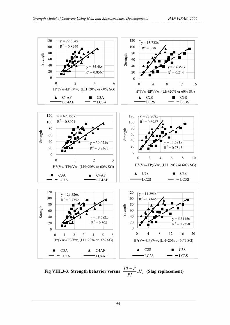
Strength Model of Concrete Using Heat and Microstructure Developments HAN VIRAK. 2006
94
y = 22.364xR2 = 0.8949
y = 35.48xR2 = 0.8567
020406080
100120
0 2 4 6H*(Vw-EP)/Vw, (LH+20% or 60% SG)
Stre
ngth
C4AF C3ALC4AF LC3A
y = 13.732xR2 = 0.781
y = 6.6351xR2 = 0.8144
0
20
40
60
80
100
120
0 4 8 12 16
H*(Vw-EP)/Vw, (LH+20% or 60% SG)
Stre
ngth
C2S C3SLC2S LC3S
y = 62.066xR2 = 0.8021
y = 39.074xR2 = 0.8361
0
20
40
60
80
100
120
0 1 2 3
H*(Vw-TP)/Vw, (LH+20% or 60% SG)
Stre
ngth
C3A C4AFLC3A LC4AF
y = 23.808xR2 = 0.6987
y = 11.591xR2 = 0.7543
020406080
100120
0 2 4 6 8 10
H*(Vw-TP)/Vw, (LH+20% or 60% SG)
Stre
ngth
C2S C3SLC2S LC3S
y = 29.526xR2 = 0.7752
y = 18.582xR2 = 0.808
0
20
40
60
80
100
120
0 1 2 3 4 5 6H*(Vw-CP)/Vw, (LH+20% or 60% SG)
Stre
ngth
C3A C4AFLC3A LC4AF
y = 11.295xR2 = 0.6645
y = 5.5115xR2 = 0.7258
020406080
100120
0 4 8 12 16 20
H*(Vw-CP)/Vw, (LH+20% or 60% SG)
Stre
ngth
C2S C3SLC2S LC3S
Fig VIII.3-3: Strength behavior versus iHPI
PPI .− (Slag replacement)

Strength Model of Concrete Using Heat and Microstructure Developments HAN VIRAK. 2006
95
y = 19.959xR2 = 0.9177
y = 32.308xR2 = 0.8898
020406080
100120
0 2 4 6H*(Vw-EP)/Vw, (LH+20%FA)
Stre
ngth
C4AF C3ALC4AF LC3A
y = 11.275xR2 = 0.8563
y = 6.0984xR2 = 0.8657
020406080
100120140
0 4 8 12 16 20
H*(Vw-EP)/Vw, (LH+20%FA)
Stre
ngth
C2S C3SLC2S LC3S
y = 72.045xR2 = 0.8896
y = 44.507xR2 = 0.9176
020406080
100120
0 0.5 1 1.5 2 2.5 3
H*(Vw-TP)/Vw, (LH+20%FA)
Stre
ngth
C3A C4AFLC3A LC4AF
y = 25.145xR2 = 0.8564
y = 13.599xR2 = 0.8655
020406080
100120140
0 2 4 6 8 10
H*(Vw-TP)/Vw, (LH+20%FA)
Stre
ngth
C2S C3SLC2S LC3S
y = 31.119xR2 = 0.8897
y = 19.224xR2 = 0.9176
020406080
100120
0 2 4 6 8
H*(Vw-CP)/Vw, (LH+20%FA)
Stre
ngth
C3A C4AFLC3A LC4AF
y = 10.861xR2 = 0.8563
y = 5.8739xR2 = 0.8656
020406080
100120140
0 4 8 12 16 20
H*(Vw-CP)/Vw, (LH+20%FA)
Stre
ngth
C2S C3SLC2S LC3S
Fig VIII.3-4: Strength behavior versus iHPI
PPI .− (Fly ash replacement)

Strength Model of Concrete Using Heat and Microstructure Developments HAN VIRAK. 2006
96
VIII.4. Data of Sumitomo Osaka and UBE-Mitsubishi cements
Table VIII.4-1 Compositions of cements provided by Sumitomo Osaka cement
Type C3S C2S C3A C4AF GypsumSpecific gravity
Fineness Modulus
LH-Used 28 53 3 10 5.0 3.24 3280 LHA 24 56 3 10 5.1 3.24 3410 LHB 25 55 3 10 5.3 3.24 3440 LHC 27 56 3 10 4.4 3.23 3380 LHD 28 54 2 10 4.6 3.24 3440 HES 63 11 9 8 6.8 3.13 4770
Table VIII.4-2 Strength of standard mortars by Sumitomo Osaka cement
Age Used A B C D HES
1 - - - - - 30.1 3 - - - - - 50.1 7 20.3 19.1 16.9 16.9 19.5 60.1 28 49.8 50.6 49.2 49.5 51 68.8 91 76.6 76.5 75.1 78.1 74.8 -
Table VIII.4-3 Cement composition of UBE-Mitsubishi corporation
C3S C2S C3A C4AF GypsumSpecific gravity
Fineness Modulus
OPC 57 17 10 8 4.6 3.16 3300 HES 66 9 9 8 6.8 3.14 4490 MH 38 42 4 10 5.2 3.21 3680 LH5 29 50 4 9 5.4 3.22 3610 LH 23 58 3 10 5.2 3.24 3470

Strength Model of Concrete Using Heat and Microstructure Developments HAN VIRAK. 2006
97
Table VIII.4-4 Strength of standard mortars by UBE-Mitsubishi corporation
Age OPC HES MH LH5 LH 1 - 27 - - - 3 28.7 47.3 20 15 10.1 7 44.8 57 28.9 22.4 13.6 28 61.8 66.2 60.5 59.3 49.7 91 66.5 - 75.1 79.3 80.1
Table VIII.4-5 Mix proportions of normal concrete by UBE-MItsubishi
Unit cement Sand Coarse aggregateCement w/c (%) Air %
kg/m3 m3/m3 m3/m3 kg/m3 m3/m3 kg/m3OPC 55 4 296 0.094 0.302 795.4 0.401 1062.4 HES 4 304 0.097 0.299 787.3 0.397 1051.6 MH 4 295 0.092 0.304 798.5 0.402 1066.6 LH5 4 293 0.091 0.304 800.7 0.404 1069.4 LH 4 291 0.090 0.305 803.1 0.405 1072.7 OPC 45 4 334.9 0.106 0.302 795.4 0.401 1062.4 HES 4 343.3 0.109 0.299 787.3 0.397 1051.6 MH 4 333.4 0.104 0.304 798.5 0.402 1066.6 LH5 4 331.3 0.103 0.304 800.7 0.404 1069.4 LH 4 329.3 0.102 0.305 803.1 0.405 1072.7 OPC 65 4 265.6 0.084 0.302 795.4 0.401 1062.4 HES 4 272.4 0.087 0.299 787.3 0.397 1051.6 MH 4 264.1 0.082 0.304 798.5 0.402 1066.6 LH5 4 262.3 0.081 0.304 800.7 0.404 1069.4 LH 4 260.6 0.080 0.305 803.1 0.405 1072.7

Strength Model of Concrete Using Heat and Microstructure Developments HAN VIRAK. 2006
98
Table VIII.4-6 Strength of normal concrete provided by UBE-Mitsubishi
Temperature 10oC 20oC 35oC Cement type w/c 45% 55% 65% 45% 55% 65% 45% 55% 65%OPC 3 15.5 11 7.36 23.5 16.6 12.4 27.2 19.8 14.1 7 31.3 22.5 16.8 37.5 26.5 20.1 41.6 29.7 23 28 43 32.1 23.7 48.3 35.7 28.2 48.5 36.8 28.2 56 49.2 38.1 29.4 50.1 37.7 29.8 49.4 37.8 28.7 91 52.5 40.7 32 51.2 39.5 30.7 50.9 38.7 29.6HES 1 14.4 8.22 4.07 21.2 13.7 7.68 28.7 19.9 13
3 31.2 21.4 15.1 38.7 26.8 19.5 43.7 32.2 23.57 41.8 30.3 22.9 46.2 34 26.7 47.4 35.7 26.614 47.5 35.3 27.2 49.9 37.2 29.3 50.6 37.9 29.1
(High Early strength)
28 51.6 39.5 30.4 52.1 39.1 30.9 51.3 38.3 29.8 91 54.1 42.3 32.8 54 40.7 32.7 51.8 39.1 30.1MH 3 10.6 6.62 4.19 15.7 10.5 7.02 18.7 13.1 8.74
7 20.2 13 7.53 24.4 16 9.76 27.2 18.4 11.8(Medium Heat) 28 36.2 24.1 14.6 43.2 30.1 21.5 43.5 31.9 23.2 56 50.7 38.2 28.4 52.7 39.8 30.4 52.6 41.4 31 91 59.5 46.7 36.8 60 47.2 37.5 59.9 47.7 37.8LH5 3 8.6 5.78 3.74 13 8.9 5.83 17.4 11.6 7.83
7 16.7 11.4 7.02 22.6 14.3 8.92 25.2 16.6 10.828 32.9 26.4 21.1 42.9 35.2 29.1 46.2 37.3 31.5
(Low Heat)
56 46.3 39.2 33.6 52.6 44.1 39 55 45.9 39.7 91 56.7 49.5 43.6 56.8 49.5 43.2 58.3 50 42.4LH 3 5.7 3.39 2.03 7.45 5.14 3.35 10.5 6.78 4.49 7 9.92 6.72 4.71 12 7.92 4.67 18.9 11.8 7.4 28 26.4 20.8 16.5 36.6 27.4 20.7 39 30.1 23.2 56 45 36.9 31.6 51.7 43.9 37.2 55 45.7 38.3 91 59.1 50.2 44 59.5 49.7 41.6 60.1 50.2 42.4

Strength Model of Concrete Using Heat and Microstructure Developments HAN VIRAK. 2006
99
Table VIII.4-7 Mix proportions of high strength concrete by UBE-Mitsubishi
Unit cement Sand Coarse aggregateCement w/c (%) Air %
kg/m3 m3/m3 m3/m3 kg/m3 m3/m3 kg/m3OPC 30 3.6 550.0 0.17 0.32 842.6 0.30 806.0 38 3.5 421.0 0.13 0.34 891.0 0.33 883.5 45 5.0 344.0 0.11 0.30 788.1 0.39 1023.0 LH5 30 3.6 550.0 0.17 0.32 852.8 0.30 806.0 38 3.6 421.0 0.13 0.34 894.5 0.33 883.5 45 5.0 344.0 0.11 0.30 794.5 0.39 1023.0 LH 30 3.7 550.0 0.17 0.32 852.8 0.30 806.0 38 3.7 421.0 0.13 0.34 894.5 0.33 883.5 45 5.1 344.0 0.11 0.30 794.5 0.39 1023.0
Table VIII.4-8 Strength of high strength concrete Provided by UBE-Mitsubishi
Temperature 10oC 20oC 35oC Cement type w/c 30% 30% 38% 45% 30% OPC 3 41.7 49.4 35.1 23.6 58 7 55.8 63.4 47.3 32.9 66.3 28 70 76.3 61.9 44.4 77.6 56 76.7 83.4 68.8 50 79.5 91 80.2 85.1 69.7 51.7 80.2 LH5 3 31.2 34 25.7 17.6 45.6 7 41.3 50.4 33.7 22.7 64.9 28 63.8 70.9 63 44.9 95.6 56 79.7 83.5 77.3 59.8 103 91 91.8 90.1 83 66.4 106 LH 3 24.5 25 22.4 17.3 37.6 7 34.3 34.6 25.7 20.6 55 28 58.9 62.8 49.4 38 92 56 77.8 78.8 70.2 57.3 98.2 91 92.9 92.5 85.3 70.5 103

Strength Model of Concrete Using Heat and Microstructure Developments HAN VIRAK. 2006
100
VIII.5. Pore effects
In section VI.3.B, the strength model was proposed with eq.70. One question is how much the gel pore and capillary pore share their effects in strength contribution.
)411316.038.121.2.( AFHCAHCSHCSHCVw
EPVwfc +−+
−
= .......................eq. 76
)411316.038.121.2( AFHCAHCSHCSHCHa ii +−+=∑ ................................eq. 77
Posing
CPGPEP ** βα += ..............................................................................................eq. 78
The equation becomes:
∑
+−
= iic HaVw
CPbGPaVwf .)**( .....................................................................eq. 79
∑−=+
ii
c
HafVwVwCPGP .** βα .........................................................................eq. 80
Using the calculated data listed in tables VIII.5-1, VIII.5-2 and VIII.5-3, the equation eq.78 is solved for α and β, we obtain:
99.000.1 == βα and .............................................................................................eq. 81
As can be seen with eq.79, the effective coefficients of GP and CP suggest that the EP is a good parameter for pore.

Strength Model of Concrete Using Heat and Microstructure Developments HAN VIRAK. 2006
101
Table VIII.5-1: Data for fictive porosity calculation for LH
Heat in Mcal/m3 Volume m3 LH Age C3A C4AF C2S C3S Water (Vw) Interlayer Gel Capillary Stregngth
w/c=0.3 7 5.044 7.672 8.398 28.456 0.308 0.040 0.044 0.153 57.0 28 5.455 8.606 14.645 30.277 0.308 0.051 0.056 0.111 81.0 7 5.326 8.106 8.399 30.207 0.308 0.042 0.046 0.147 59.0 14 5.719 9.038 12.950 31.694 0.308 0.050 0.055 0.115 77.3 28 5.976 9.625 16.930 32.560 0.308 0.057 0.063 0.089 100.2 91 6.268 10.277 21.065 33.442 0.308 0.063 0.070 0.062 116.4 w/c=0.45 7 3.978 5.957 5.952 22.707 0.328 0.031 0.034 0.209 33.9 14 4.350 6.921 9.219 23.683 0.328 0.037 0.041 0.185 45.3 28 4.552 7.466 12.949 24.100 0.328 0.043 0.047 0.162 56.5 91 4.711 7.900 17.735 24.344 0.328 0.050 0.055 0.134 78.1 7 4.031 5.982 5.952 23.078 0.328 0.031 0.034 0.207 27.8 14 4.459 7.099 9.219 24.016 0.328 0.037 0.041 0.183 42.5 28 4.668 7.728 13.072 24.315 0.328 0.043 0.048 0.159 61.3 91 4.784 8.110 19.343 24.409 0.328 0.052 0.058 0.124 83.1 w/c=0.6 7 2.983 4.397 4.372 17.191 0.321 0.023 0.025 0.232 13.4 28 3.479 5.799 9.607 17.918 0.321 0.032 0.035 0.197 36.3 7 2.986 4.397 4.372 17.259 0.321 0.023 0.025 0.232 13.9 14 3.356 5.309 6.772 17.848 0.321 0.028 0.031 0.214 23.4 28 3.498 5.849 9.607 17.929 0.321 0.032 0.036 0.196 38.7 91 3.530 6.028 15.166 17.934 0.321 0.040 0.044 0.166 50.3

Strength Model of Concrete Using Heat and Microstructure Developments HAN VIRAK. 2006
102
Table VIII.5-2: Data for fictive porosity calculation for OPC
Heat in Mcal/m3 Volume m3 Age C3A C4AF C2S C3S Water (Vw) Interlayer Gel Capillary Stregngth
w/c=0.3 7 15.562 4.840 4.185 44.092 0.304 0.047 0.057 0.106 75.48 14 16.083 5.048 4.580 46.392 0.304 0.050 0.060 0.095 83.82 28 16.509 5.215 4.851 48.136 0.304 0.052 0.063 0.086 91.68 91 17.051 5.421 5.162 50.209 0.304 0.054 0.065 0.077 96.18 7 17.153 5.352 4.789 50.722 0.304 0.054 0.065 0.077 84.25 14 18.107 5.738 5.428 54.102 0.304 0.058 0.070 0.060 91.74 28 18.894 6.048 5.914 56.649 0.304 0.061 0.074 0.047 100.42 91 19.959 6.456 6.527 59.827 0.304 0.065 0.079 0.031 108.32 w/c=0.45 7 14.145 4.344 3.803 43.082 0.323 0.045 0.055 0.133 54.90 14 15.441 4.944 4.860 46.261 0.323 0.050 0.061 0.113 62.48 28 16.301 5.344 5.591 48.030 0.323 0.053 0.064 0.100 71.98 91 17.180 5.766 6.351 49.483 0.323 0.056 0.068 0.088 77.05 w/c=0.6 7 10.823 3.253 2.803 33.365 0.317 0.035 0.042 0.171 33.70 14 12.104 3.877 3.774 35.779 0.317 0.039 0.047 0.153 39.85 28 12.676 4.227 4.534 36.476 0.317 0.041 0.050 0.144 46.53 91 12.918 4.408 5.005 36.642 0.317 0.042 0.051 0.140 51.56

Strength Model of Concrete Using Heat and Microstructure Developments HAN VIRAK. 2006
103
Table VIII.5-3: Data for fictive porosity calculation for HES
Heat in Mcal/m3 Volume m3 Age C3A C4AF C2S C3S Water (Vw) Interlayer Gel Capillary Stregngth
w/c=0.3 7 11.119 5.125 3.059 49.280 0.305 0.048 0.058 0.107 85.60 14 11.536 5.314 3.345 51.757 0.305 0.051 0.061 0.096 92.95 28 11.892 5.476 3.549 53.725 0.305 0.053 0.063 0.088 96.90 91 12.362 5.690 3.796 56.152 0.305 0.055 0.066 0.078 97.67 7 12.473 5.678 3.539 56.504 0.305 0.055 0.066 0.078 90.65 14 13.173 6.014 3.978 59.927 0.305 0.059 0.070 0.063 96.39 28 13.788 6.309 4.328 62.691 0.305 0.062 0.074 0.051 104.74 91 14.662 6.729 4.792 66.311 0.305 0.066 0.078 0.034 111.87 w/c=0.45 7 9.781 4.401 2.785 44.385 0.315 0.043 0.052 0.137 57.01 14 10.416 4.737 3.258 46.935 0.315 0.046 0.055 0.125 62.24 28 10.930 5.011 3.605 48.799 0.315 0.049 0.058 0.115 67.61 91 11.608 5.380 4.046 50.972 0.315 0.051 0.061 0.104 69.67 w/c=0.6 7 8.232 3.675 2.281 36.996 0.317 0.036 0.043 0.169 36.78 14 8.801 4.036 2.872 38.684 0.317 0.039 0.046 0.158 40.62 28 9.130 4.258 3.229 39.467 0.317 0.040 0.048 0.152 44.42 91 9.349 4.431 3.522 39.832 0.317 0.041 0.049 0.148 47.20

Strength Model of Concrete Using Heat and Microstructure Developments HAN VIRAK. 2006
104
REFERENCES [1]. Maekawa K., Chaube R. and Kishi T., Modelling of Concrete Performance, ISBN
0-419-24200-7, London and New York, 1999. [2]. Taylor H.F.W., Cement Chemistry, 2nd edition, 1997. [3]. De Larrard F. Concrete mixture proportioning, ISBN 0 419 23500 0, London and
New York, 1999. [4]. A. M. Neville CBE and J. J. Brooks, Concrete Technology, 1990. [5]. Dupain R., Lanchon R. and Saint-Arroman J.C. Granulats, sols, cements et betons,
ISBN 2-7135-2064-9, Paris, 2000. [6]. Lessard M. and Aitcin P.C. in Les betons a hautes performances, ISBN
2-85978-187-0, Paris, p.221-241, 1992. [7]. Bentz D.P., Modeling the Influence of Limestone Filler on Cement Hydration Using
CEMHYD3D, USA. [8]. Suzuki, Y., Harada, S., Maekawa, K. and Tsuji, Y., Evaluation of adiabatic
temperature rise of concrete measured with the new testing apparatus, Concrete Library of JSCE, 1989, No. 13, 71-83.
[9]. Suzuki, Y., Tsuji, Y., Maekawa, K. and Okamura, H., Quantification of hydration-heat generation process of cement in concrete, Concrete Library of JSCE, 1990, No. 16, 111-24.
[10]. Kishi. T and Maekawa. K, Multi-component model for hydration heating of blended cement with blast furnace slag and fly ash, Proceeding of JSCE, No. 550/Vol-33, 1996.
[11]. Neville, A. M., Properties of Concrete, ISBN 0-582-23070-5. [12]. Sakai. E.,Yamada. K and Ohta. A., Molecular Structure and Dispersion-Adsorption
Mechanisms of Comb-Type Superplasticizers Used in Japan, Journal of Advanced Concrete Technology Vol. 1, No.1, 16-25, April 2003.
[13]. Ferraris. F. Chiara, "Concrete Mixing Methods and Concrete Mixers: State of Art", Journal of Research of the National Institute of Standards and Technology, Vol. 106, No. 2, 391-399, March-April 2001.
[14]. Scrivener. K. L. and Gariner. E. M., "Microstructural gradients in cement paste around aggregate particles", Material Research Symposium Proc., 114, pp. 77-85 (1988).
[15]. Bentz. D. P, Replacement of "coarse" cement particles by inert fillers in low w/c ratio concretes II. Experimental validation, Cement Concrete Research, vol.35, No. 1, pp.185-188, 2005.
[16]. Bentur, A., Goldman, A. and Cohen, M.D. (1988). Mater. Res. Soc. Sym. Proc. 114, 97.

Strength Model of Concrete Using Heat and Microstructure Developments HAN VIRAK. 2006
105
[17]. Kishi, T et al, Multi-component heat calculation code: developed 2005. [18]. 小田部 裕一、複合水和発熱モデルの一般化と水和相識形成に着目した強度
発現モデルの開発。 [19]. Kishi, T. and Otabe, Y., Universal Modeling for Hydration Heat Generation of
Arbitrarily Blended Cementitious Materials Based on Multi-Component System, International RILEM-JCI Seminar on Concrete Durability and Service Life Planning, Concrete life'06, 14-16 March 2006, Ein-Brokek, Dead Sea, Israel.
[20]. 小田部裕一、岸利治、論文:初期空隙における水和物形成に基づいた強度発
現性の評価、コンクリート工学年次論文集、Vol. 27, No 1, 2005. [21]. 小田部 裕一、岸 利治、コンクリートの品質予測・施工管理支援に向けた
水和反応・強度発現モデルの開発、生産研究 第 57 巻 第二号抜刷、2005年 3 月。
[22]. KEN W. DAY, Concrete Mix Design, Quality Control and Specification, 2nd edition, ISBN 0-419-24330-5, 1999.
[23]. Dalgleish, B. J. and Pratt, P. L., Fractographic Studies of microstructural development in hydrated Portland cement, Journal of Material science, No 17, pp. 2199-2207, 1982.
[24]. Test records (of cement chemical compositions provided by manufacturers) [25]. UBE-Mitsubishi cement corporation, technical reports.
ASTM Standards:
[26]. C 29-97 Standard Test Method for Bulk Density ("Unit Weight") and Voids in Aggregate.
[27]. C172-97 Standard Test Method for Sampling Freshly Mixed Concrete. [28]. C 39-96 Standard Test Method for Compressive Strength of Cylindrical Concrete
Specimens. [29]. C109-98 Standard Test Method for Compressive Strength of Hydraulic-Cement
Mortars (Using 2-in. or [50-mm] Cube Specimens) [30]. C349-97 Standard Test Method for Compressive Strength of Hydraulic-Cement
Mortars (Using Portions of Prisms Broken in Flexure) [31]. C348-97 Standard Test Method for Flexural Strength of Hydraulic-Cement Mortars [32]. C128-97 Standard Test Method for Specific Gravity and Absorption of Fine
Aggregate. [33]. C 136-96a Standard Test Method for Sieve Analysis of Fine and Coarse
Aggregate. [34]. C 192-95 Standard Practice for Making and Curing Concrete Test Specimens in the
laboratory.

Strength Model of Concrete Using Heat and Microstructure Developments HAN VIRAK. 2006
106
[35]. C494-98 Standard Specification for Chemical Admixtures for Concrete [36]. C 171-97 Standard Specification for Sheet Materials for Curing Concrete. [37]. C 618-98 Standard Specification for Coal Fly Ash and Raw or Calcined Natural
Pozzolan for Use as a Mineral Admixture in Concrete. [38]. Standard Specification for Ground Granulated Blast-Furnace Slag for Use in
Concrete and Mortar