Strengthening farm operators’ capacity for climate change

adaptation

Armen R. Kemanian Associate Professor

The Pennsylvania State University

Agroclimatology Project Directors Meeting 18 December 2016

Foreword

It is March 25, 2012 in Central Pennsylvania. March has been unusually warm, and Jeanne the Farmer is getting ready for planting corn ahead of schedule. The soil condition is perfect, the planter is loaded with seed, the fertilizer is in the tank. Yet, Jeanne is pondering if planting corn this early risk exposing the crop to a late frost under the guise of an eventual bumper crop. Jeanne decides to go ahead and plant corn, after all she already paid for a long season hybrid. Four weeks later 60% of the crop is killed by a late frost. Jeanne needs to decide now if it is worth replanting corn, and if so if a short season hybrid should be used, to avoid late maturation and frost again, now in the fall. But, are seeds available? She also heard that climate forecasters predict a strong chance of a drier than usual summer. What does that mean for risk of drought or corn borer damage? There is also strong competition for machinery, and getting a good contractor for the planting timely is becoming challenging. There was a chance of losing that crop to a frost, there were other options - perhaps planting early only 50% of the area? Decision points, uncertainty. Can science and technology help Jeanne deal with the havoc brought up by climate variability? Can the losses be avoided or reduced with a strategy that recognize in advance the existing risks? We think so.

This project is about improving the capacity of farmers to deal with the uncertainty of climate change and variability in agricultural production.

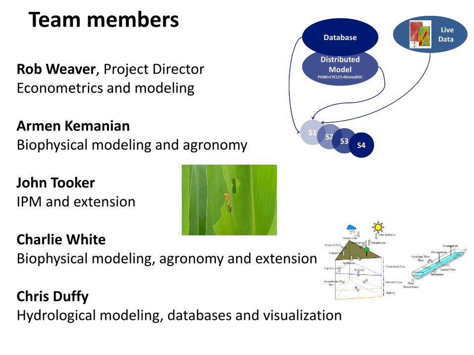
Team members

Rob Weaver, Project Director Econometrics and modeling Armen Kemanian Biophysical modeling and agronomy John Tooker IPM and extension Charlie White Biophysical modeling, agronomy and extension Chris Duffy Hydrological modeling, databases and visualization

Framework

Local CCR Realization

Events

CC Predictions & Scenarios Multiple Time Scales

Predictions & Scenarios

Materials & Supplies

Farm labor

Custom services

Predictions & Scenarios

Output prices Input prices

Local Supply

Realization Events

Local Price Realization

Events

Lon

g-term

/ Me

diu

m-term

/ Pre

-seaso

n / In

tra-seaso

n

Mu

ltiple

ne

sted

time

scale p

lann

ing &

action

Farm Options for Adaptation

Farm Actions: Adaptation

Strategic management problem: Multiple climate and market processes with feedback

Op

tion

s

Info

rma

tio

n Q

ua

lity

• Advanced planning for land use

• Adaptive capacity

– Short-run for field operation choice and timing

– Medium-term for shifts in long-term plans

• Market conditions reflect both realized and anticipated agroecosystem and climate conditions

• Market volatility spans quantity and prices

Farm level decision salient features

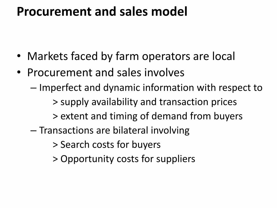
• Markets faced by farm operators are local

• Procurement and sales involves – Imperfect and dynamic information with respect to

> supply availability and transaction prices

> extent and timing of demand from buyers

– Transactions are bilateral involving

> Search costs for buyers

> Opportunity costs for suppliers

Procurement and sales model

• Developed to predict prices from bilateral transactions

• Provides basis for farm-level scenario analysis that incorporates salient features of farm-level procurement and sales settings.

Market level model

Provides production and environmental impacts data for econometrics and integrated models

Model helps managing complex reality

Ernst et al 2016 Field Crops Research 186, 107-116

Wh

eat

yie

ld, k

g h

a-1

Actual yield Attainable yield

Climatic Index

Climate, soil, genetics, management and

economic interactions

1. Water balance (includes irrigation, water potential based)

2. Crop growth (includes nutrient uptake, optimization theory)

3. Model plant communities (competition, polycultures)

4. Carbon and nutrient balance (saturation theory)

5. Apply management practices (tillage, fertilization, …)

Cycles notes

Inputs: database + conditioning of Meteorological data Soils data Management data

𝒘 =𝐴

𝐸=

λ 𝒄𝒂 − Γ∗ − 𝑹𝒅 𝒌

𝑟𝑔

1

𝐷

𝒘 ≈λ 𝒄𝒂 − Γ∗

𝒓𝒈

1

𝐷

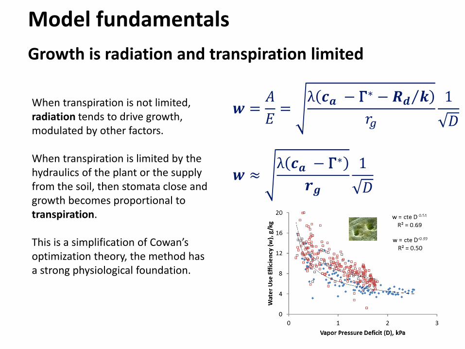
Model fundamentals

Growth is radiation and transpiration limited

When transpiration is not limited, radiation tends to drive growth, modulated by other factors. When transpiration is limited by the hydraulics of the plant or the supply from the soil, then stomata close and growth becomes proportional to transpiration. This is a simplification of Cowan’s optimization theory, the method has a strong physiological foundation.

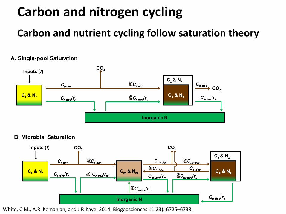
White, C.M., A.R. Kemanian, and J.P. Kaye. 2014. Biogeosciences 11(23): 6725–6738.

Carbon and nitrogen cycling

Carbon and nutrient cycling follow saturation theory

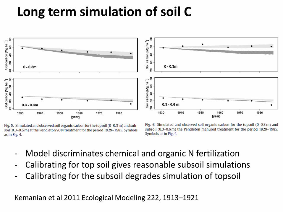
- Model discriminates chemical and organic N fertilization - Calibrating for top soil gives reasonable subsoil simulations - Calibrating for the subsoil degrades simulation of topsoil Kemanian et al 2011 Ecological Modeling 222, 1913–1921

Long term simulation of soil C

Corn Rye Soy Wheat Canola Corn Rye Soy Wheat Alfalfa Crop Rotation:

Compost/Fertilizer

0

20

40

60

80

100

1998 1999 2000 2001 2002 2003 2004

Soil

NO

3- a

t 5

-10

cm

(mg

N/k

g)

Inorganic Fertilizer

Compost

Compost/Fertilizer Compost/Fertilizer Compost/Fertilizer

0

0.1

0.2

0.3

1998 1999 2000 2001 2002 2003 2004

N2

O D

en

itri

fica

tio

n

(kg

N/h

a/d

ay)

Inorganic Fertilizer

Compost

0

0.2

0.4

0.6

0.8

1

1998 1999 2000 2001 2002 2003 2004

Nit

rate

Le

ach

ing

(kg

N/h

a/d

ay)

Inorganic Fertilizer Compost

Simulation of N dynamics

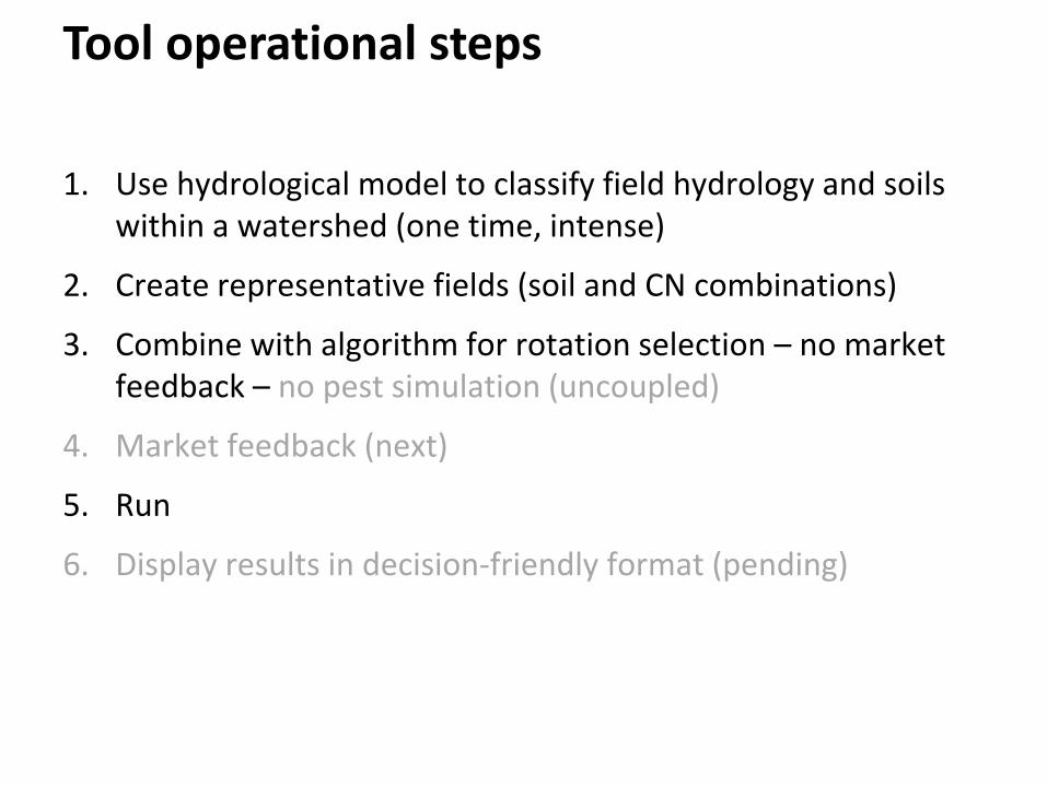
1. Use hydrological model to classify field hydrology and soils within a watershed (one time, intense)

2. Create representative fields (soil and CN combinations)

3. Combine with algorithm for rotation selection – no market feedback – no pest simulation (uncoupled)

4. Market feedback (next)

5. Run

6. Display results in decision-friendly format (pending)

Tool operational steps

Tools

GIS - Geographic Information System

TIN - Domain Decomposition: Triangular Irregular Net

FVM - Finite Volume Method

PDE - Partial Differential Equations

PDAE - Differential-Algebraic Equations

C. Duffy, L. Leonard and L. Shu

PIHM

Conestoga

Conestoga

DEM

DEM

Forcing data

Climate forcing

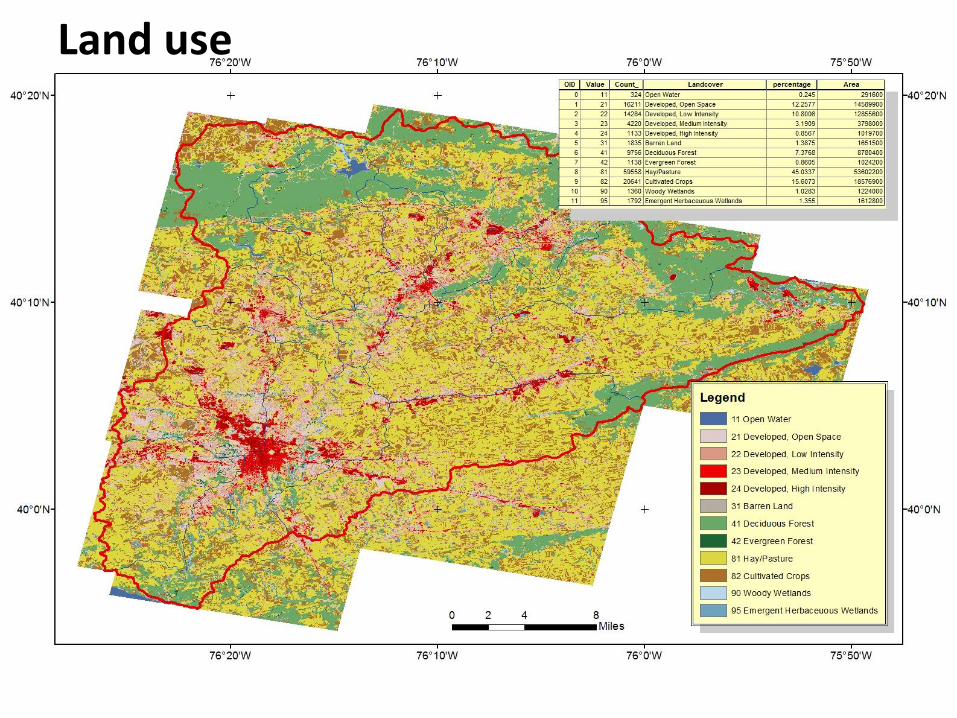
Land use

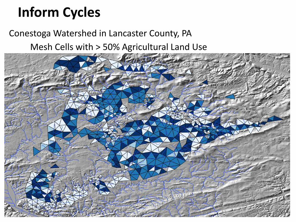
Conestoga Watershed in Lancaster County, PA

Mesh Cells with > 50% Agricultural Land Use

Inform Cycles

Interested in limitations to crop productivity, informed by PIHM • Interrogated average behavior of mesh cells by month • Focused on drivers of transpiration

0.00

0.50

1.00

1.50

2.00

2.50

3.00

3.50

0.00 5.00 10.00 15.00 20.00 25.00

Ave

rage

Tra

nsp

irat

ion

in A

ugu

st (

mm

/day

)

Average August Water Storage (Saturated + Unsaturated) m

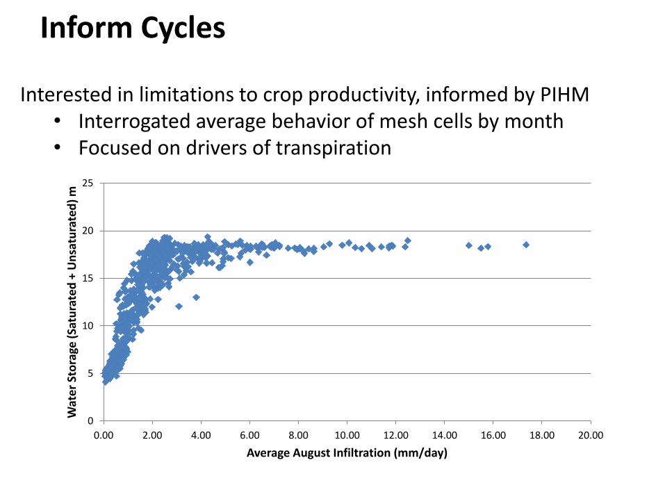
Inform Cycles

0

5

10

15

20

25

0.00 2.00 4.00 6.00 8.00 10.00 12.00 14.00 16.00 18.00 20.00

Wat

er

Sto

rage

(Sa

tura

ted

+ U

nsa

tura

ted

) m

Average August Infiltration (mm/day)

Interested in limitations to crop productivity, informed by PIHM • Interrogated average behavior of mesh cells by month • Focused on drivers of transpiration

Inform Cycles

0.00

0.50

1.00

1.50

2.00

2.50

3.00

3.50

0.00 2.00 4.00 6.00 8.00 10.00 12.00 14.00 16.00 18.00 20.00

Ave

rage

Au

gust

Tra

nsp

irat

ion

(m

m/d

ay)

Average August Infiltration (mm/day)

Interested in limitations to crop productivity, informed by PIHM • Interrogated average behavior of mesh cells by month • Focused on drivers of transpiration

Inform Cycles

Using CN to regulate infiltration rate and Cycles crop yield output

y = 0.975x

y = 0.8763x

y = 0.6795x

y = 0.5212x

y = 0.2683x

0

5

10

15

20

25

30

0 5 10 15 20 25 30

Cro

p B

iom

ass

wit

h N

ew C

urv

e N

um

be

r

(Mg/

ha)

Crop Biomass with Curve Number = 60 (Mg/ha)

CN = 89

CN = 95

CN = 97

CN = 98

CN = 99

0.00

0.50

1.00

1.50

2.00

2.50

3.00

3.50

0.00 1.00 2.00 3.00 4.00 5.00A

vera

ge A

ugu

st T

ran

spir

atio

n (

mm

/day

) Average August Infiltration (mm/day)

Curve Number 99 97 60

Use Cycles

Decision Support Tool Example

- Set up price series for winter wheat, maize and soybean - Establish planting time window for each crop - Establish soil condition for planting - Add rotational constrains Run (for two soils in this case)

Adding a biomass crop buffer strip greatly reduces N near stream

Why not C-PIHM? Computational demand Maize biomass and soil nitrate concentration in a 5 ha watershed Simulation of 10 years may take 4 to 6 hours

Next steps

1. Use hydrological model to classify field hydrology and soils within a watershed (one time, intense)

2. Create representative fields (soil and CN combinations)

3. Combine with algorithm for rotation selection – no market feedback – (add) pest simulation (currently uncoupled)

4. Market feedback (create “farms” with fields)

5. Run

6. Display results in decision-friendly format (pending)

7. Web-based prototype? This is the ultimate goal

Thank you!

NIFA award# 2014-68002-21768

(Most likely no time for questions)