strengthening the experimenters toolbox: statistical estimation of

Strengthening the Experimenter’s Toolbox: StatisticalEstimation of Internal Validity

Luke Keele Penn State UniversityCorrine McConnaughy Ohio State UniversityIsmail White Ohio State University

Experiments have become an increasingly common tool for political science researchers over the last decade, particularlylaboratory experiments performed on small convenience samples. We argue that the standard normal theory statisticalparadigm used in political science fails to meet the needs of these experimenters and outline an alternative approach tostatistical inference based on randomization of the treatment. The randomization inference approach not only providesdirect estimation of the experimenter’s quantity of interest—the certainty of the causal inference about the observed units—but also helps to deal with other challenges of small samples. We offer an introduction to the logic of randomization inference,a brief overview of its technical details, and guidance for political science experimenters about making analytic choiceswithin the randomization inference framework. Finally, we reanalyze data from two political science experiments usingrandomization tests to illustrate the inferential differences that choosing a randomization inference approach can make.

Experimentation has been a growth industry inpolitical science over the last decade or so. Thisgrowth reflects an interest in making valid causal

inferences about political phenomena. Randomly assign-ing subjects either to receive or not to receive a treat-ment that represents a causal factor of interest enables re-searchers to employ the assumption that they have equiv-alent groups, with the exception of the groups’ recep-tion of the treatment. Thus, the cause of any observeddifferences across the groups in the outcome of inter-est is validly ascribed to the treatment—but not withoutsome uncertainty. Because random assignment deliversequivalence in expectation, there remains a chance in anyone experiment that the groups were different on theoutcome of interest before treatment. Thus, the experi-menter is left with the question of how certain it is thatany observed difference is due to the treatment, and not

Luke Keele is Associate Professor, Department of Political Science, 211 Pond Lab, Penn State University, University Park, PA 16802([email protected]). Corrine McConnaughy is Assistant Professor, Department of Political Science, 2018 Derby Hall, Ohio State University,Columbus, OH 43210 ([email protected]). Ismail White is Assistant Professor, Department of Political Science, 2008 DerbyHall, Ohio State University, Columbus, OH 43210 ([email protected]).

Authors are in alphabetical order. For helpful comments and discussion, we thank Jake Bowers, Sanford Gordon, Kosuke Imai, CindyKam, Walter Mebane, David Nickerson, Jasjeet Sekhon, Nicholas Valentino, Lynn Vavrek, and seminar participants at the University ofMichigan, Columbia University, and Princeton University. We also thank James Fowler and Cindy Kam for generously sharing their data.For research assistance, we thank Kevin Duska. A previous version of this article was presented at the 2008 annual meeting of the MidwestPolitical Science Association, the 2008 annual meeting of the American Political Science Association, Boston, MA, and the 2010 Visions inMethodology Conference, Iowa City, IA. Replication materials are available at http://dvn.iq.harvard.edu/dvn/dv/ljk. An online supplementcontains further details about specific randomization tests as well as information about the data used.

to the chance of random assignment, itself. We engage inthis article the question of how to characterize this un-certainty through statistical tests and do so while payingattention to the frequency with which political science ex-periments rely upon small, nonrandom samples, typicallytermed convenience samples. We thus offer an overviewof the logic of randomization inference and its basic im-plementation, as well as guidance about when particularstatistical tools might be most helpful and appropriate.Randomization inference uses random assignment as thestatistical basis for inference to offer estimates of un-certainty about whether observed outcomes under onerandom treatment assignment might have been observedunder an alternative random allocation of the treatment.It is a departure from commonly used classical statis-tical tests in the frequentist framework, which typicallyrely on an assumption of random sampling and involve a

American Journal of Political Science, Vol. 56, No. 2, April 2012, Pp. 484–499

C© 2012, Midwest Political Science Association DOI: 10.1111/j.1540-5907.2011.00576.x

484

THE EXPERIMENTER’S TOOLBOX 485

p-value as an estimate of the uncertainty about whethera sample is representative of a population. Using classicalinference also relies on the assumption that the test statis-tic follows some parametric distribution such as the t orNormal. In political science applications where the cen-tral inferential task is connecting a sample to a specifiedpopulation, the classical approach makes sense. In the ex-perimental context, it very often does not.1 Classic infer-ential tools do not provide direct estimates of the experi-menter’s quantity of interest—uncertainty about internalvalidity—and their assumptions of random sampling andparametric distributions can seem unwarranted or eventroubling given the samples used in some experiments.The randomization inference approach enables the ex-perimenter to proceed without such assumptions. It alsooffers tests that can address a number of common ana-lytic challenges faced by political science experimenters.Yet, invoking the randomization inference frameworkdoes not necessarily entail the use of new statistical tech-niques. Indeed, a number of randomization tests can beapproximated by standard (normal theory) tests whensample (cell) sizes are large enough. A firm understand-ing of the randomization inference approach, however,clearly delineates which standard tests are appropriate andwhen.

Randomization inference is not new. In fact, the con-cept dates back to the basic theory of randomization for-mulated by Fisher (1935). These tests have been largelyabsent, however, from experimental methodology in po-litical science. We conducted a JSTOR search for all articlesthat contained the word “experiment” published between1995 and 2007 in the American Political Science Review,the American Journal of Political Science, and the Journal ofPolitics. This search returned 258 articles. We did not finda single example of randomization inference. We expect,however, that practitioners offered an informed choicebetween standard approaches and the randomization in-ference approach will find the latter useful.2

1 There are ways to recast experiments and randomization as sam-pling mechanisms to provide a basis for classical statistical infer-ence. The most coherent story is to treat the subjects as a populationand assume that random assignment of treatment forms a samplingmechanism for that population. Another possibility is to assumethat the convenience sample is a random sample from some un-known or hypothetical population (Lehmann and Romano 2005).

2 This is not to say that randomization tests are totally unknownto political scientists. Hansen and Bowers (2008) investigate andadvocate the utility of randomization tests using a political scienceapplication. Ho and Imai (2006) provide another example with apolitical application. These all appear in statistics journals, whichunderscores the rarity of these tests in political science. We knowof one article published in the main disciplinary journals that usesrandomization tests to analyze an experiment: Fowler and Kam

To convey the intuition of the randomization infer-ence framework, we walk the reader through a simpleexample before moving on to the technical details of theapproach. We cover not only the technicalities of simplehypothesis testing, but also the estimation of treatmenteffects and confidence intervals. We then illustrate theuse and implications of randomization inference withtwo published experiments highlighting the differencesbetween the inferences that would be made from thesedata using randomization inference rather than standardtests.

Principles of RandomizationInference: An Example

Before providing a formal description of randomizationtests, we start with an example to illustrate the logicand implementation of the randomization inference ap-proach. We introduce with this example both the gen-eral intuition of randomization inference and the use ofa rank-based test, which is possible but not necessarywithin the randomization framework. Consider an ex-periment where we select seven students to play a dictatorgame with a computer program which asks them to al-locate 100 dollars between themselves and a charitabledonation.3 Three of the students are randomly chosento receive the treatment, a prime expected to make themmore altruistic. If the treatment is effective, we wouldexpect that the students who receive it would give awaymore of their money. If there is no effect of the treatment,we would expect no such difference across the two sets ofstudents. In other words, we are interested in testing thefollowing null hypothesis:

H0: The prime has no effect on amount given,

against our alternative:

Ha: The prime has a positive effect on amount given.

Relying on the standard toolkit of the political scientist,we might translate these expectations into a t-test com-paring the observed mean difference in dollars given toa null of no mean difference. We would then calculatea p-value using the critical value from a t-distribution.Note this implies the assumption that the test statisticfollows a t-distribution. As an alternative, we can derivethe statistical test from the randomization of treatment

(2007), an article that fell just outside the time bounds of ourinitial JSTOR search.

3 This example is adapted from one in Sprent and Smeeton (2007).

486 LUKE KEELE, CORRINE MCCONNAUGHY, AND ISMAIL WHITE

TABLE 1 Possible Combinations of Ranks inTreatment Group

1,2,3 1,2,4 1,2,5 1,2,6 1,2,71,3,4 1,3,5 1,3,6 1,3,7 1,4,51,4,6, 1,4,7 1,5,6 1,5,7 1,6,72,3,4 2,3,5 2,3,6 2,3,7 2,4,52,4,6 2,4,7 2,5,6 2,5,7 2,6,73,4,5 3,4,6 3,4,7 3,5,6 3,5,73,6,7 4,5,6 4,5,7 4,6,7 5,6,7

assignment and avoid the parametric assumption entailedin the use of the t-distribution.

Our expectation in this example, again, is that treatedstudents should give away more than nontreated students.The best evidence that the prime increased altruistic be-havior would be if the three students who received thetreatment rank 1, 2, and 3 in terms of the amount givenaway. So we might ask: what is the probability that thethree students in the treatment group would happen torank 1, 2, and 3 in terms of the amount given away ifthe null hypothesis were true, and, in fact, there was noeffect of the prime? To develop a probability statementabout this hypothesis that hinges on the composition ofthe treatment and control groups—the feature that wasassigned by a random process—we turn to basic combi-natorics. Knowing that the number of ways of selecting robjects from a set of n is n!/[r !(n − r )!] tells us that thereare 35 ways to select three students from a set of seven.Table 1 contains all the possible combinations of ranksthat we could observe for our set of treated subjects, andrandom allocation of treatment determines the probabil-ity for each of these cell entries. Seeing in the table thatour best evidence outcome is 1 of 35 possible treatment-group compositions tells us that there is a 1/35 ≈ 0.0286chance that we would observe the best evidence case if thenull were true. That is, the chance that random assign-ment alone will produce this exact outcome is 1/35. Thisp-value indicates that the best evidence outcome enablesus to be fairly confident that the prime has an effect onstudent behavior in our divide-the-dollar game.4

We can make this approach to hypothesis testingmore general by introducing a summary statistic thatenables us to translate ranks into a single measurementof the outcome among the treatment subjects. One pos-sible statistic for this purpose is the sum of the ranksfor the treated subjects. This statistic will be lower if the

4 If we had a two-sided alternative hypothesis, we would doublethe resultant p-value. For details on other methods for calculatingtwo-sided p-values, see Lehmann (1975).

treated subjects are generally higher in their giving thanthe control subjects, and higher if they are not.5 Usingthis statistic, we can answer the question of what thechance is of observing an outcome of a specific degree (orsmaller/larger) among the treatment subjects. For exam-ple, suppose the outcome we observed among the treatedsubjects was the ranks 1, 2, and 7. Our summary statisticwould be 10 (1 + 2 + 7 = 10). This seems close to the“best evidence” outcome we just considered, where thesum of the ranks would be 1 + 2 + 3 = 6, but is it closeenough to be convincing evidence of a treatment effect?To answer this question, we work out the probability ofobserving a rank sum statistic of the same amount orless by returning to our enumeration of all 35 possiblecombinations of the three ranks and calculating the ranksum for each combination. Four of the 35 possible rankcombinations produce a sum of 10, three more producea sum of 9, two result in a sum of 8, one set sums to 7,and another to 6. Thus, under random assignment, thechance of observing an outcome like the one we did orsmaller would be p = 11/35 ≈ 0.314. Put another way,if the prime has no effect, we could expect to see a valuefor the summed ranks as low as or lower than the one weobserved 31 out of every 100 times we randomly assignedthe treatment to these particular subjects. Using the tradi-tional hypothesis testing threshold of .05, the p-value wecalculated would not allow us to reject the null hypothesis;the observed outcome did not provide sufficient evidencethat the prime had an effect on our subjects’ behavior.Thus, the p-value in a randomization test is calculated asthe probability of observing a test statistic as large as orlarger than the observed test statistic.

Note that the interpretation of the p-values in thisexample references the information we believe the po-litical science experimenter is after: the probability thatthe result observed among his or her specific set of ex-perimental subjects can be explained away by the chanceconstitution of the treatment groups under one allocationof treatment. Randomization inference explicitly focuseson local inference, endeavoring to compare the responsesthat the subjects studied exhibited under one randomallocation of treatment to the unobserved responses thesame individuals would have displayed under an alternaterandom allocation of treatment. We do not need to assertthese subjects are any sort of sample from any known pop-ulation. An inference of this type is valid for any type ofsample and may be particularly sensible for conveniencesamples. We are able to make statistical inferences because

5 Note the inverse relationship is due to the direction of ourranking—that those who gave away more were given lower val-ues for their ranks (highest giver being ranked 1, etc.). Havingdirectionality—and attending to it—is what is important here.


we can use the randomization of the treatment to create ameaningful probability distribution for the null hypoth-esis and can calculate a p-value for any combination ofvalues that we might observe in the experiment withoutever using a parametric distribution.

Principles of RandomizationInference: Formal Matters

In this section, we offer a formal outline of randomizationinference. We begin with the basic mechanics of testingthat the treatment is completely without effect, includingexplanations of exact tests and sharp null hypotheses.We discuss the process of choosing an appropriate teststatistic, including considerations about using rank-basedtests. Of course, calculating the p-value for rejecting thenull of no treatment effect is only one statistical quantityof interest, so we also discuss methods for generatingconfidence intervals and point estimates. And we discussthe possibility of approximating randomization inferencetests with standard parametric tests, including caveatsabout turning to these statistical tools.

The basic mechanics of a statistical test built on therandomization inference framework include the same el-ements as any statistical test: data, a null hypothesis, a teststatistic, and a distribution of the test statistic under thenull hypothesis. The derivation of the last element, thenull distribution, however, is unique to randomizationtests. To provide a formal derivation of the null distri-bution, we first define T as a random vector that assignssubjects to either the treatment or control group. To illus-trate, if the first, third, and fourth subjects out of sevensubjects are selected to receive the treatment, T wouldhave the following form: (1,0,1,1,0,0,0).

Next, we denote the quantity y as a vector of theoutcomes for the subjects, and we define the teststatisticas

S = f (y, T). (1)

That is, the test statistic, S, is the result of a function,f , that operates on both the observed outcomes and thetreatment assignment. In the example in the first section,S took the form of the summed ranks for the treatmentgroup. The function f and the test statistic S can take sev-eral possible forms; we discuss some of those possibilitiesin greater detail in following sections.

We further denote all possible responses under thetreatment as � with elements si . This � contains all out-comes under all possible realizations of T. In our earlierexample, summing each of the entries in Table 1 would

form � for the experiment. We use � to calculate theprobability of observing a value of S of a particular sizesi or larger (or smaller, depending on the direction ofour expectations) if the null hypothesis were true. Thisp-value is the sum of the randomization probabilities thatlead to those referenced values of S, relative to all possiblevalues of S:

p = P r (S ≥ si |H0) =∑

I (S ≥ si )

|�| , (2)

where I (·) is an indicator function, and | · | denotes thecardinality of a set. Generating p-values in this way im-plies that randomization tests are exact . A statistical testis exact when the p-value is an always exact calculation of�, where � is the probability of making a Type I error—rejecting the null hypothesis when it is true. � is, of course,an important piece of information in the decisions wemake about statistical evidence. Recall that using the con-ventional 0.05 significance level for hypothesis testing, forexample, reflects an intention to set � to 0.05. Exactnessis thus an attractive property of randomization tests. Incomparison, the actual probability of a Type I error willdiffer from � under a traditional parametric test if thetest statistic fails to meet any of the test assumptions. Forexample, if T , the test statistic in the t-test, diverges froma t-distribution, perhaps due to outliers in the data, theprobability of a Type I error using that test will differfrom �.6

As promising as the randomization inference ap-proach to hypothesis testing with experimental dataseems, there is one caveat, albeit a practical one. For largesamples, the number of possible outcomes can be quitelarge and, even with modern computing, the time re-quired to compute an exact p-value can be lengthy. Forsuch situations, we can simulate the distribution of nulloutcomes and derive approximate exact p-values. Withlarge samples, these simulated tests have been shown tovery closely approximate the exact tests. In fact, in exam-ples where the entire null distribution can be elaborated,approximate tests based on simulation produce accurateinferences even when the number of simulations is con-siderably smaller than the total number of permutations.7

6 The same logic holds for confidence intervals. We specify thecoverage for a confidence interval by selecting 1 − �. In parametrictests, a failure to meet the distributional assumption can cause thisto be untrue.

7 There are several exceptions. Fisher’s exact test for a binary out-come and a binary treatment has a closed-form solution, as thepermutation distribution follows a hypergeometric distribution.Other tests with closed-form solutions are the Mantel and Haen-szel test and the d statistic of Hansen and Bowers (2009).


The mechanics of randomization inference mecha-nism bear repeating. Probability enters our calculationsonly through randomization of the treatment and doesnot rely on any parametric probability distribution orsampling mechanism. That is, the inference is entirelydesign-based—assuming only random allocation of unitsto experimental conditions—and invokes no modelingassumptions external to the study design. Here, the nulldistribution is completely known. Moreover, the p-valuesdirectly translate into the experimenters’ original quan-tity of interest: the probability that what they observe asevidence of a treatment effect can be explained away bythe chance process that assigned their observed subjectsinto treatment and control groups.

The Sharp Null

The randomization inference paradigm we have outlinedwas developed by Fisher (1935), who advocated makinginferences about treatment effects through a test of thesharp null hypothesis. Under the sharp null hypothesis,we test whether the treatment effect is zero for all units.The potential outcomes framework helps clarify the dis-tinct nature of the sharp null hypothesis. First, we notethat for each unit i observed in the experiment, the in-dicator Ti = t, t ∈ {0, 1}, records the randomly assignedtreatment status. Each unit then has a potential outcomefor each treatment condition, which we denote as Yi (t).In potential outcomes notation, if the sharp null hypoth-esis holds, then Yi (1) = Yi (0). That is, treatment statusis irrelevant to each individual subject’s outcome; eachwould exhibit the exact same potential outcome underthe treatment as he or she would when not treated. Thisapproach is different from the approach developed byNeyman (1923), which tests hypotheses about the aver-age treatment effect (ATE). Under Neyman’s formula-tion, the null hypothesis is that the ATE is zero, whichmay occur even if the treatment effect is not zero for allsubjects—some subjects exhibiting a positive effect andothers a negative effect could produce an average of “nodifference” across the treated and control groups. Whilethe Neyman approach is certainly sensible and widelyembraced, there are compelling reasons to adopt Fisher’sapproach to hypothesis testing. Most notably, the p-valuefrom a test of the sharp null is accorded special status dueto its assumption-free nature. As Rosenbaum (2002b, 27)notes:

In the theory of experimental design, a specialplace is given to the test of the hypothesis thatthe treatment is entirely without effect. The rea-son is that, in a randomized experiment, this test

may be performed virtually without assumptionsof any kind, that is, relying on the random as-signment of treatments.

The experimenter need only assert about his or herdata that he or she did, in fact, perform a randomizedexperiment. It is unnecessary even to make what Rubin(1986) called the “stable unit-treatment value assump-tion” or SUTVA, which is commonly needed to pro-ceed with other tests. SUTVA asserts that the potentialoutcomes under treatment or control for each unit arefixed and notably do not depend on the treatment statusof other units. The test of the sharp null is valid evenif SUTVA is violated, which can easily occur throughinterference—when the outcome for one unit is affectedby the treatment status of other units (Rosenbaum 2007).8

And while Fisher’s approach enables the analyst to pro-ceed without assumptions, tests of average effects re-quire additional assumptions even for simple hypothesistesting.9

This does not mean that tests based on p-values areof greater practical importance than point estimates andconfidence intervals. Some, particularly Bayesians, havequestioned the value of hypothesis tests, sharp or oth-erwise, and p-values (Gill 1999) and have argued thatconfidence intervals and point estimates along with simu-lations and assessments of practical significance are morevaluable than a test of the null hypothesis (Gelman andHill 2006). Certainly it is true that many researchers willwish to know more about what their results suggest aboutthe substantive significance of their treatments. As wediscuss further below, estimates of this sort require addi-tional assumptions. When the researcher has any doubtabout those assumptions, testing the sharp null seemsall the more important and useful. Recent work does,however, allow one to retain the randomization infer-ence framework but relax the assumption that the treat-ment effect is the same for all units in the experiment(Rosenbaum 2003, 2007). We give a very brief introduc-tion to these techniques later. In what follows, then, whenwe refer to a hypothesis test, we mean Fisher’s versionof these tests. As we discuss later, in large samples thedistinction between the Fisher and Neyman approachesvanishes.

8 Note that Rubin (1986) argued that Fisher’s framework automati-cally implied a special form of SUTVA held, rather than that SUTVAcould be violated.

9 In brief, the Neyman approach involves first using the mean dif-ference as an unbiased estimator of the causal estimand. The analystnext finds an unbiased or upwardly biased estimator for the vari-ance of the average causal effect. An appeal to the central limittheorem allows the analyst to form a confidence interval for theaverage causal effect based on these estimated quantities.


Test Statistics

A range of valid test statistics is available to the exper-imenter within the randomization framework. That is,one has choices about f , the function that operates ontreatment assignment and observed outcomes to produceS, a test statistic. An ideal choice will produce a test statis-tic that distinguishes between the null and alternativehypothesis. In statistical terms, we want a powerful teststatistic, one that will have an extreme value if the nullhypothesis is false. It is difficult to offer a more specificgeneral recommendation for choosing a test statistic be-cause there are many alternative hypotheses, and no onetest statistic is powerful in reference to all of them. We thusreview here three test statistics that might be useful—eachof which compares how the distribution of the potentialoutcomes under the alternative hypothesis differs fromthe distribution under the null—and provide some com-mentary on why each might be chosen. Importantly, wediscuss the limitation of statistics as the basis for guidancein choosing a test statistic and the role that theory andsubstantive judgment must play.

Tests based on differences in means are a familiar toolfor comparisons across treated and control groups and areavailable within the randomization inference framework.We might choose the average difference across the treat-ment and control groups:

�A = 1

nT

∑Yi (1) − 1

nC

∑Yi (0) = y1 − y0 (3)

where nC is the number of units in the control group andnT is the number of units in the treatment group.10 Whilethis statistic is attractive for its ease of interpretation, itis sensitive to outliers and will have low power if thereare larger differences in the tails of the two distributions.Other similar test statistics are possible. For example, onemight use the test statistic from the t-test.

A transformation before comparing average levelsacross treatment and control can produce other usefulstatistics. For example, taking natural logarithms of theoutcomes and estimating as follows,

�M = 1

nT

∑ln(Yi (1)) − 1

nC

∑ln(Yi (0)) (4)

produces a statistic that we can interpret as a constantmultiplicative treatment effect (Imbens and Rubin 2008).Such a transformation might be especially attractive whena constant additive effect might (incorrectly) suggest po-tential outcomes for some units that are outside the sub-

10 Note this test statistic does not imply a test of an average treatmenteffect. It is still a test of the sharp null hypothesis, where it is assumedthe effect of the treatment is constant. Why this is true will be clearwhen we discuss point estimation.

stantively meaningful bounds of the outcome measure,as in a count of something like income or the number ofvotes cast.

Test statistics based on ranks of the outcome data arealso common. As we illustrated with our example in thefirst section, the outcomes are transformed to integersthat rank where they fall in the distribution of observedvalues, and the test statistic is the sum of these ranksin the treatment group. Examples of these tests includethe Wilcoxon rank-sum test for comparison of a controlgroup and a single treated group and the Kruskal-Wallistest for comparison of multiple treated groups.11 Ranktests are attractive for their ability to detect differenceseven in the presence of long-tails and/or outliers. Rank-based randomization tests are also convenient becausethey are widely available in statistical software.

Questions of how we might interpret differences be-tween a test using the test statistic based on means and thetest statistic based on ranks and how we choose the mostappropriate test statistic involve subtle issues worth ex-ploring. Suppose a researcher uses both the mean-basedand rank-based test statistic. She finds that the p-valuefor the mean-based test statistic is well above the standard0.05 threshold, while the rank-based statistic’s p-value isbelow 0.05. What does this imply, other than there aresome responses to treatment that are “unusual”? Answer-ing that question involves thinking through what “un-usual” means, which likely depends on the substance andtheory in question. First, suppose the experiment wasbased on a formal theory that predicted that all agentsshould behave the same, perhaps that all subjects shouldbe equally generous in a divide-the-dollar game. In the ob-served outcomes, however, a few subjects were unusuallygenerous. The question for the experimenter is whethershe believes a few instances of extreme generosity are dueto aberrant subject-level responses or should be treatedas particularly important information about the theory’svalidity. Perhaps she has some evidence to suggest thatthe extreme values were due to some subjects not fullyunderstanding the experiment’s instructions. In this case,she might choose a rank-based test, such that the extrem-ity of those values does not exert much influence on thetest of a treatment effect. If, however, she has nothing tosuggest that those observations were not “true” values,she might think that the mean-based test statistic bettercaptures what the data have to say about the theoreti-cal prediction. Similarly, think about the challenges facedby political psychology experimenters working on ques-tions of priming and accessibility. Many use the responsetime—the time in milliseconds it takes for a subject to

11 Details on both of these tests are available in the appendix.


perform a categorization task—as a measure of accessi-bility. When the treatment is a prime, it should make therelevant construct more accessible and reduce responsetimes to the corresponding items in the task. The difficultyis that any brief distraction can wildly inflate the responsetime since it is measured in milliseconds. One commonstrategy in the literature is to simply drop such obser-vations (see Nelson, Clawson, and Oxley 1997). A rank-based statistic provides the experimenter with a princi-pled method for dealing with the outliers that invariablyoccur when response times are the outcome of interest,enabling them to keep the observations but reduce theirinfluence on the test of the treatment’s effect. In gen-eral, we suggest that it can be useful to compare a statisticbased on means to one based on ranks. Differences suggesta need to make judgments about the nature of unusualobservations.

Estimation

Thus far, we have only discussed the calculation of anexact p-value for a test of the sharp null hypothesis. Ofcourse, many experimenters wish to say something aboutthe size of the treatment effect given the evidence in theirdata. That is, experimenters are likely to be interested ina point estimate for the treatment effect and a confidenceinterval for that point estimate. Both interval and pointestimation are both possible within the randomization in-ference framework. Both, however, require assumptionsthat were unnecessary for calculating the exact p-value inthe test of no effect.

Two additional assumptions are needed for inter-val and point estimation. First, we must assume SUTVAholds. Second, we must make an assumption about thenature of response to the treatment. Rosenbaum (2002b)refers to this second assumption as a model of effects.Rosenbaum (2002b, chap. 5) outlines a number of differ-ent models of effects, but the most widely used model ofeffects is that of a constant-additive effect, which is the ef-fect implied by a linear model. That is, we assume that thetreatment raises the response of each unit by a constantamount: Yi (1) = Yi (0) + � , where � is the treatmenteffect.12

A 100(1 − �)% confidence interval for the additivetreatment effect, � , is formed by “inverting” a series of100(1 − �)% level tests. In short, we conduct a seriesof hypothesis tests with nonzero values of �0 using the

12 The model of the effects may or may not correspond to the teststatistic. For example, the constant-additive model of effects maybe used with the average difference of means test statistic as well asthe rank-sum test statistic.

same method we outlined in the second section and keepthe values not rejected at the value of � we have cho-sen, typically 0.05. For each test, we exploit the fact thatYi (1) = Yi (0) + � under the null to adjust each observedoutcome by �0 and then conduct a test of the sharp null hy-pothesis. The calculated p-values enable us to specify thevalues at the endpoints of the 100(1 − �)% confidence in-terval. This method of interval estimation is perhaps bestunderstood with a simple example. Say we conduct anexperiment testing whether social pressure affects inten-tion to vote. We measure intention to vote with a 7-pointscale, with higher values indicating a higher propensity tovote. We observe 12 subjects, six of whom are randomlyexposed to a social pressure cue. We observe the followingoutcomes:

Treatment Group = (7, 7, 5, 4, 6, 5)Control Group = (1, 4, 5, 1, 5, 5).

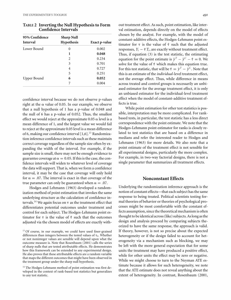
We use the absolute difference in means across the treatedand control units as our test statistic. Thus, our test statis-tic has a value of approximately 2.17. First, we test theusual sharp null hypothesis that the treatment effect iszero. To calculate an exact p-value, again, we comparethe number of times a test statistic value as large as orlarger than the one we observe occurs relative to the uni-verse of test statistic values computed from all possiblepermutations of the outcomes we observed. In this case,there are 924 possible ways to form a treatment group ofsix subjects from a pool of 12. Comparing the observedtest statistic value of 2.17 to the values from the 924 per-mutations, we find that the exact p-value is 0.002, andthus we reject the sharp null hypothesis that the treat-ment effect is zero. Next, to construct our confidenceinterval, we begin by assuming a model of constant ad-ditive effects. We use that model to test a series of sharpnull hypotheses, testing that �0 = 1 and then �0 = 2 andso on. In this example, we specify values of �0 in incre-ments of 1. We then compute adjusted responses accord-ing to our model of effects, using the equation Yi − �0Ti .Note that, here, adjustment is to the observed out-come, which is defined as Yi = Ti Yi (1) + (1 − Ti )Yi (0).In sum, we subtract the value of �0 for each null hy-pothesis from the treatment-group observations andthen calculate the test statistic and corresponding exactp-value in the same way we did with the observed data.We form the confidence interval from the hypothesis testsfor the values of �0 where we do not reject at a chosenlevel of �. The results from this iterative process are inTable 2.

We form a 95% confidence interval for our treatmenteffect, meaning we find the values of �0 where we rejectthe null at � = .05. Given the discrete nature of exactp-values, we may be unable to form a precise 100(1 − �)%


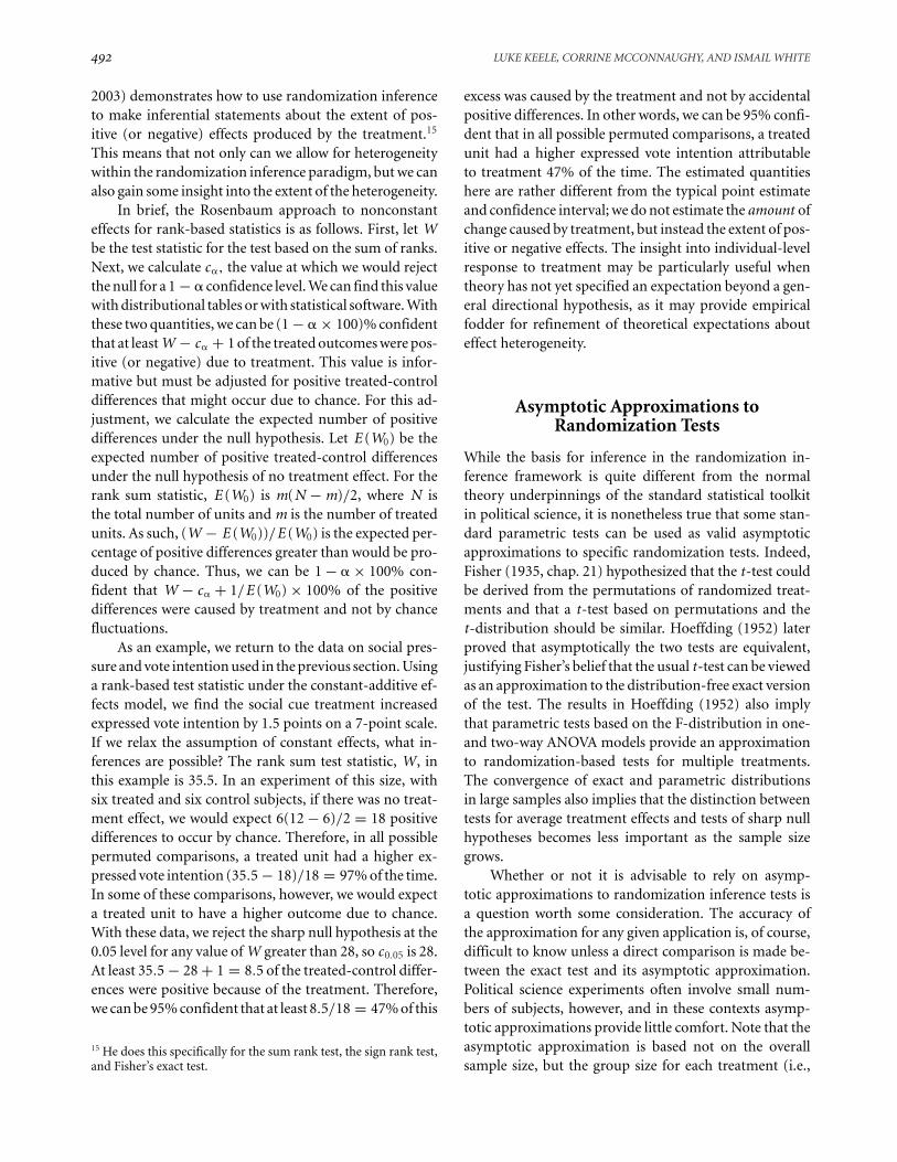
TABLE 2 Inverting the Null Hypothesis to FormConfidence Intervals

95% Confidence Sharp NullInterval Hypothesis Exact p-value

Lower Bound 0 0.0021 0.0482 0.2343 0.7014 0.7275 0.251

Upper Bound 6 0.0527 0.004

confidence interval because we do not observe p-valuesright at the � value of 0.05. In our example, we observethat a null hypothesis of 1 has a p-value of 0.048 andthe null of 6 has a p-value of 0.052. Thus, the smallesteffect we would reject at the approximate 0.05 � level is amean difference of 1, and the largest value we would failto reject at the approximate 0.05 level is a mean differenceof 6, making our confidence interval [1,6].13 Randomiza-tion inference confidence intervals such as these maintaincorrect coverage regardless of the sample size often by ex-panding the width of the interval. For example, if thesample size is small, there may not be enough evidence toguarantee coverage at � = 0.05. If this is the case, the con-fidence intervals will widen to whatever level of coveragethe data will support. That is, when we form a confidenceinterval, it may be the case that coverage will only holdfor � = .07. The interval is exact in that coverage of thetrue parameter can only be guaranteed when � = .07.

Hodges and Lehmann (1963) developed a random-ization method of point estimation that invokes the sameunderlying structure as the calculation of confidence in-tervals.14 We again focus on � as the treatment effect thatdifferentiates potential outcomes under treatment andcontrol for each subject. The Hodges-Lehmann point es-timator for � is the value of � such that the outcomesadjusted via the chosen model of effects are exactly with-

13 Of course, in our example, we could have used finer-graineddifferences than integers between the tested values of �0. Whetheror not noninteger values are sensible will depend upon what theoutcome measure is. Note that Rosenbaum (2001) calls the seriesof sharp nulls that are tested attributable effects. He demonstrateshow this framework can be extended to any experimental design.He also proves that these attributable effects are a random variablethat maps the different outcomes that might have been observed inthe treatment group under the sharp null hypothesis.

14 The Hodges-Lehmann method of point estimation was first de-veloped in the context of rank-based test statistics but generalizesto any test statistic.

out treatment effect. As such, point estimation, like inter-val estimation, depends directly on the model of effectschosen by the analyst. For example, with the model ofconstant-additive effects, the Hodges-Lehmann point es-timator for � is the value of � such that the adjustedresponses, Yi − � Ti , are exactly without treatment effect.Thus, if equation (3) is the test statistic, the estimatingequation for the point estimate is yT − yC − � = 0. Wesolve for the value of � which makes this equation true.For this test statistic, that will be � = yT − yC . Note thatthis is an estimate of the individual-level treatment effect,not the average effect. Thus, while difference in meansacross treated and control groups is necessarily an unbi-ased estimator for the average treatment effect, it is onlyan unbiased estimator for the individual-level treatmenteffect when the model of constant-additive treatment ef-fects is true.

While point estimation for other test statistics is pos-sible, interpretation may be more complicated. For rank-based tests, in particular, the test statistic has a less directcorrespondence with the point estimate. We note that theHodges-Lehmann point estimator for ranks is closely re-lated to test statistics that are based on a difference inmedians and refer the interested reader to Hodges andLehmann (1963) for more details. We also note that apoint estimate of the treatment effect is not sensible forall experimental designs, particularly the more complex.For example, in two-way factorial designs, there is not asingle parameter that summarizes all treatment effects.

Nonconstant Effects

Underlying the randomization inference approach is thenotion of constant effects—that each subject has the sameresponse to being treated. Political scientists testing for-mal theories of behavior or theories of psychological pro-cesses might be most comfortable with the constant ef-fects assumption, since the theoretical mechanism is oftenthought to be identical across (like) subjects. As long as thedesign and analysis proceed by comparing subjects the-orized to have the same response, the approach is valid.If theory, however, is not so precise about the expectedheterogeneity or if the design failed to account for het-erogeneity via a mechanism such as blocking, we maybe left with the more general expectation that for someunits the treatment may have produced a positive effect,while for other units the effect may be zero or negative.While we might choose to turn to the Neyman ATE es-timate because it allows for such heterogeneity, we notethat the ATE estimate does not reveal anything about theextent of heterogeneity. In contrast, Rosenbaum (2001,


2003) demonstrates how to use randomization inferenceto make inferential statements about the extent of pos-itive (or negative) effects produced by the treatment.15

This means that not only can we allow for heterogeneitywithin the randomization inference paradigm, but we canalso gain some insight into the extent of the heterogeneity.

In brief, the Rosenbaum approach to nonconstanteffects for rank-based statistics is as follows. First, let Wbe the test statistic for the test based on the sum of ranks.Next, we calculate c�, the value at which we would rejectthe null for a 1 − � confidence level. We can find this valuewith distributional tables or with statistical software. Withthese two quantities, we can be (1 − � × 100)% confidentthat at least W − c� + 1 of the treated outcomes were pos-itive (or negative) due to treatment. This value is infor-mative but must be adjusted for positive treated-controldifferences that might occur due to chance. For this ad-justment, we calculate the expected number of positivedifferences under the null hypothesis. Let E (W0) be theexpected number of positive treated-control differencesunder the null hypothesis of no treatment effect. For therank sum statistic, E (W0) is m(N − m)/2, where N isthe total number of units and m is the number of treatedunits. As such, (W − E (W0))/E (W0) is the expected per-centage of positive differences greater than would be pro-duced by chance. Thus, we can be 1 − � × 100% con-fident that W − c� + 1/E (W0) × 100% of the positivedifferences were caused by treatment and not by chancefluctuations.

As an example, we return to the data on social pres-sure and vote intention used in the previous section. Usinga rank-based test statistic under the constant-additive ef-fects model, we find the social cue treatment increasedexpressed vote intention by 1.5 points on a 7-point scale.If we relax the assumption of constant effects, what in-ferences are possible? The rank sum test statistic, W, inthis example is 35.5. In an experiment of this size, withsix treated and six control subjects, if there was no treat-ment effect, we would expect 6(12 − 6)/2 = 18 positivedifferences to occur by chance. Therefore, in all possiblepermuted comparisons, a treated unit had a higher ex-pressed vote intention (35.5 − 18)/18 = 97% of the time.In some of these comparisons, however, we would expecta treated unit to have a higher outcome due to chance.With these data, we reject the sharp null hypothesis at the0.05 level for any value of W greater than 28, so c0.05 is 28.At least 35.5 − 28 + 1 = 8.5 of the treated-control differ-ences were positive because of the treatment. Therefore,we can be 95% confident that at least 8.5/18 = 47% of this

15 He does this specifically for the sum rank test, the sign rank test,and Fisher’s exact test.

excess was caused by the treatment and not by accidentalpositive differences. In other words, we can be 95% confi-dent that in all possible permuted comparisons, a treatedunit had a higher expressed vote intention attributableto treatment 47% of the time. The estimated quantitieshere are rather different from the typical point estimateand confidence interval; we do not estimate the amount ofchange caused by treatment, but instead the extent of pos-itive or negative effects. The insight into individual-levelresponse to treatment may be particularly useful whentheory has not yet specified an expectation beyond a gen-eral directional hypothesis, as it may provide empiricalfodder for refinement of theoretical expectations abouteffect heterogeneity.

Asymptotic Approximations toRandomization Tests

While the basis for inference in the randomization in-ference framework is quite different from the normaltheory underpinnings of the standard statistical toolkitin political science, it is nonetheless true that some stan-dard parametric tests can be used as valid asymptoticapproximations to specific randomization tests. Indeed,Fisher (1935, chap. 21) hypothesized that the t-test couldbe derived from the permutations of randomized treat-ments and that a t-test based on permutations and thet-distribution should be similar. Hoeffding (1952) laterproved that asymptotically the two tests are equivalent,justifying Fisher’s belief that the usual t-test can be viewedas an approximation to the distribution-free exact versionof the test. The results in Hoeffding (1952) also implythat parametric tests based on the F-distribution in one-and two-way ANOVA models provide an approximationto randomization-based tests for multiple treatments.The convergence of exact and parametric distributionsin large samples also implies that the distinction betweentests for average treatment effects and tests of sharp nullhypotheses becomes less important as the sample sizegrows.

Whether or not it is advisable to rely on asymp-totic approximations to randomization inference tests isa question worth some consideration. The accuracy ofthe approximation for any given application is, of course,difficult to know unless a direct comparison is made be-tween the exact test and its asymptotic approximation.Political science experiments often involve small num-bers of subjects, however, and in these contexts asymp-totic approximations provide little comfort. Note that theasymptotic approximation is based not on the overallsample size, but the group size for each treatment (i.e.,


the cell size; Lehmann 1975). And while the impetus forasymptotic approximations stemmed from the practicalconstraints of exact calculations, modern computing en-ables relatively quick exact calculations for even largerexperiments.

We see one other more nuanced reason to approachasymptotic approximations with caution. While there arevalid asymptotic approximations for many randomiza-tion tests, simple alterations of the analysis can renderthese approximations incorrect. For example, a bivariateregression model with treatment status as the indepen-dent variable provides inferences about treatment effectsidentical to those from the t-distribution, which is anapproximation of the randomization distribution. Onemight suspect that a multivariate regression model withadded covariates therefore provides a similar approxima-tion. Freedman (2008a, 2008b) proves, however, that thisis not the case. He demonstrates that for the estimationof treatment effects, the multiple regression estimator isbiased. The bias goes to zero as the sample size increasesand is typically trivial. The bias arises from the fact thatthe linear model assumes treatment effects are constantacross units (Freedman 2008a, 2008b). The real concern,however, is that the multiple regression model may ei-ther overstate or understate the estimates’ precision bysurprisingly large amounts. Why should this be the case?Recall that the usual Gauss-Markov assumptions for thelinear regression model hold that the error terms are inde-pendent and identically distributed (IID). The difficultyis that this assumption is directly contradicted by thepotential outcomes model of an experiment used in ran-domization inference: the errors will vary with treatmentby definition, making the error variance nonconstant.This nonconstant error variance in a regression model isusually referred to as heteroskedasticity. Given that het-eroskedasticity is the barrier to using multivariate regres-sion to approximate the randomization distribution, onemight assume that the solution is some form of robuststandard errors or perhaps a multiplicative model of het-eroskedasticity. Neither of these options, however, is thesolution. Lin (2010) demonstrates that for the multivari-ate regression model to approximate the randomizationdistribution, one must use a fully saturated model. That is,one must include the full set of treatment-covariate inter-actions. So while one can use the multivariate regressionmodel to approximate the randomization distribution, itrequires alterations to the model that are not obvious.

A similar mistake can be made if logistic regressionis used to approximate the randomization distribution.For experiments with a binary treatment and outcome,randomization inference is possible with either Fisher’sexact test or the sign test based on binomial sampling.

One might assume that a logistic regression model is anappropriate approximation to the exact test. Freedman(2008c) demonstrates that this is not the case. Again, thedifficulty arises from the fact that only the treatment isstochastic, while the logistic regression model assumesthe outcome is a random binomial process.

Given the possible complications, we strongly em-phasize that care must be taken with asymptotic approxi-mations. While there are valid approximations available,subtle alterations in the mode of testing can result in teststhat are not approximations of the randomization distri-bution. We have outlined two examples where unless theanalyst is careful what may seem like a harmless asymp-totic approximation actually does not approximate theinference justified by randomization. If the asymptoticapproximation is used, however, randomization infer-ence brings greater clarity to the parametric test. Eventhough the distribution used is parametric, the justifica-tion for that distribution stems from random assignment.The inference remains local and is focused on uncertaintyabout the treatment, and not on sampling from a largerpopulation.

Parametric Assumptions and Power

Next, we use a comparison of nonparametric confidenceintervals with standard parametric confidence intervals toillustrate an important point about the way in which theapplication of randomization inference techniques canenable the data from an experiment to speak more clearlyabout the evidence produced by the experiment. To formparametric confidence intervals, one must assume thatthe data follow a particular distribution. When the sam-ple size is small, this essentially adds information to thedata, which will result in confidence intervals that may beoverly narrow and fail to maintain correct coverage (Im-bens and Rosenbaum 2005). The parametric assumptionis analogous to using an informative Bayesian prior withthe data, and informative priors are most likely to influ-ence our answer when sample sizes are small. In com-parison, the confidence intervals from Fisher-style ran-domization tests maintain correct coverage regardless ofhow many observations are used. The exact 100(1 − �)%confidence set for the treatment effect estimate will al-ways maintain its stated coverage of 100(1 − �)%. Thatincludes, importantly, that when the data do not con-tain enough information, the interval may achieve thiscoverage by becoming infinite in length (Imbens andRosenbaum 2005). That is, we may find that there areno values of the sharp null hypothesis where we are ableto reject at a chosen confidence level. This, we think, isan attractive feature of these nonparametric confidence


intervals: they reveal whether additional data are requiredto increase the power of the test in order to say somethingsubstantively meaningful.

Consider an example from an experiment we con-ducted. In the experiment, subjects in the treatment groupviewed a story from the local newspaper about a mugging.The control group was exposed to a story from the samelocal newspaper about changes to the iPhone. Subjectswere then asked to rate whites and African Americans on aset of stereotype items. The difference in subjects’ attribu-tion of stereotype traits to whites and African Americansmeasures whether the treatment caused subjects to rateAfrican Americans lower relative to whites when primedon the topic of crime. Our experiment had 19 subjectsin the control condition and 22 subjects in the treatmentcondition. If we proceed with a standard parametric anal-ysis based on the t-test, the difference in mean ratings is−1.3. That is, subjects in the treatment condition ratedAfrican Americans 1.3 points lower than whites on thestereotype scale. The normal theory confidence intervalfor this estimate is [−2.47, −0.19]. The point estimate forthe treatment effect from the rank sum test is seeminglysimilar in substantive terms, at−1.5, with an exact p-valueof 0.004. The confidence interval for the nonparametricestimate, however, is [−∞, 0]. Using the randomizationtest in this case reveals that there is not enough informa-tion in the data to say anything more about the treatmenteffect other than it is negative. To be more specific aboutthe treatment effect would require us to invoke a para-metric assumption or repeat the experiment with moresubjects.

This somewhat minor point raises controversial is-sues in statistical inference. A Bayesian might argue thatin small samples informative priors are necessary sincethe data have little to tell us. Better here to rely on sub-stantive knowledge and impose a prior. In fact, the para-metric t-test can be thought of as a Bayesian estimate withan uninformative prior. The difficulty is that, as we havedemonstrated in this example, this obscures important in-formation about statistical power. In our example, we seethat by assuming the data are distributed normally addsinformation to the data resulting in confidence intervalsthat are overly narrow unless the parametric assumptionis correct. With the nonparametric test, we observe thatthe treatment effect is clearly negative, and we can rejectthe null that the sharp null is zero, but we would concludethat to learn more about the treatment effect requires alarger sample size. While one might be willing to defend aflat prior, the parametric assumption, here, is troubling.We argue it is better to know that the experiment as con-ducted does not have enough power to rule out a varietyof null hypotheses and to know for future iterations of

the experiment that a larger number of subjects is neededfor more precise inferences.

Statistical Tests with RandomizationInference for Political Science

Given that a randomization test needs to be built from theprobability model used for treatment assignment, thereare a wide variety of tests to fit various experimental de-signs. Clearly we cannot review them all here. The inter-ested reader and practitioner will likely need to seek outvarious additional sources. Though texts on nonpara-metric statistics should cover many of the possible tests,they often fail to show the link between each test and therandomization mechanism in the experimental design.One notable exception is Lehmann (1975), who derivescommon rank-based nonparametric tests from randomassignment of treatment. Higgins (2003) is a recent textthat provides the randomization-based justification fortests in a wide variety of experimental designs, includingboth mean- and rank-based test statistics. In the statisticsliterature, the rank-based test statistics that we discussedearlier are quite popular, and thus many lucid discussionsof randomization inference there (see Rosenbaum 2002b,chap. 2) focus almost entirely on rank-based tests. Theappendix to this article contains a basic introduction torank-based tests, including those for two-way factorialdesigns. The latter may be of particular interest as wehave found that coverage of randomization tests for two-way factorial designs is quite rare, while such designs arerelatively common in the social sciences.

Examples from Political ScienceExperiments

Having laid out our case for randomization tests, we nowturn to applying these tests to two datasets from polit-ical science experiments. We use a dataset from Fowlerand Kam (2007), whose published results represent arare example of the use of randomization tests in po-litical science, and part of a dataset produced by White(2003) from which results have not been previously pub-lished. Both experiments were performed on conveniencesamples—one relying entirely on student subjects and theother recruiting both students and nonstudent adults. Wecompare the results from standard statistical tests to thosefrom randomization tests. In addition to offering a moredirect estimate of the type of uncertainty that concernsthe experimentalist, we find that randomization tests can


produce p-values that would lead to different substantiveconclusions.

Partisan Generosity

Fowler and Kam (2007) performed a series of experimentsto test a set of hypotheses about individuals’ propen-sity to give to others. The authors brought student sub-jects into a laboratory environment and asked them toplay a dictator game, wherein each subject was givena set of 10 lottery tickets and asked to divide the tick-ets between themselves and an anonymous recipient. Bymanipulating the identity of the anonymous recipient,Fowler and Kam intended to test for differences in givingthat could be attributed to the effects of social identities.Thus, three experimental conditions were employed, thetreatment being the identity of the recipient: no iden-tifying information, registered Democrat, or registeredRepublican.

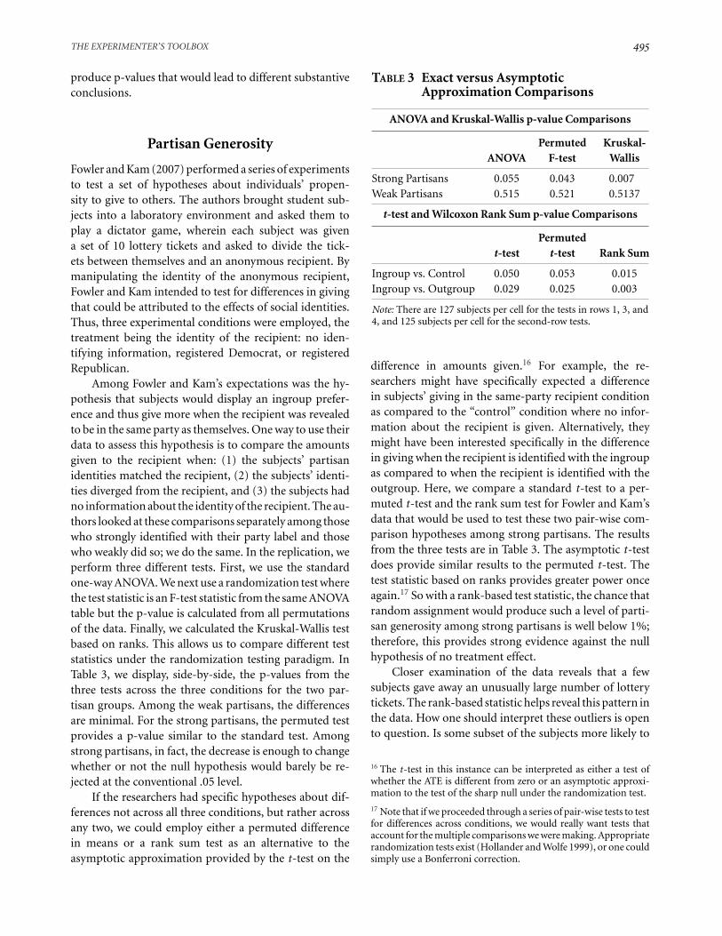
Among Fowler and Kam’s expectations was the hy-pothesis that subjects would display an ingroup prefer-ence and thus give more when the recipient was revealedto be in the same party as themselves. One way to use theirdata to assess this hypothesis is to compare the amountsgiven to the recipient when: (1) the subjects’ partisanidentities matched the recipient, (2) the subjects’ identi-ties diverged from the recipient, and (3) the subjects hadno information about the identity of the recipient. The au-thors looked at these comparisons separately among thosewho strongly identified with their party label and thosewho weakly did so; we do the same. In the replication, weperform three different tests. First, we use the standardone-way ANOVA. We next use a randomization test wherethe test statistic is an F-test statistic from the same ANOVAtable but the p-value is calculated from all permutationsof the data. Finally, we calculated the Kruskal-Wallis testbased on ranks. This allows us to compare different teststatistics under the randomization testing paradigm. InTable 3, we display, side-by-side, the p-values from thethree tests across the three conditions for the two par-tisan groups. Among the weak partisans, the differencesare minimal. For the strong partisans, the permuted testprovides a p-value similar to the standard test. Amongstrong partisans, in fact, the decrease is enough to changewhether or not the null hypothesis would barely be re-jected at the conventional .05 level.

If the researchers had specific hypotheses about dif-ferences not across all three conditions, but rather acrossany two, we could employ either a permuted differencein means or a rank sum test as an alternative to theasymptotic approximation provided by the t-test on the

TABLE 3 Exact versus AsymptoticApproximation Comparisons

ANOVA and Kruskal-Wallis p-value Comparisons

Permuted Kruskal-ANOVA F-test Wallis

Strong Partisans 0.055 0.043 0.007Weak Partisans 0.515 0.521 0.5137

t-test and Wilcoxon Rank Sum p-value Comparisons

Permutedt-test t-test Rank Sum

Ingroup vs. Control 0.050 0.053 0.015Ingroup vs. Outgroup 0.029 0.025 0.003

Note: There are 127 subjects per cell for the tests in rows 1, 3, and4, and 125 subjects per cell for the second-row tests.

difference in amounts given.16 For example, the re-searchers might have specifically expected a differencein subjects’ giving in the same-party recipient conditionas compared to the “control” condition where no infor-mation about the recipient is given. Alternatively, theymight have been interested specifically in the differencein giving when the recipient is identified with the ingroupas compared to when the recipient is identified with theoutgroup. Here, we compare a standard t-test to a per-muted t-test and the rank sum test for Fowler and Kam’sdata that would be used to test these two pair-wise com-parison hypotheses among strong partisans. The resultsfrom the three tests are in Table 3. The asymptotic t-testdoes provide similar results to the permuted t-test. Thetest statistic based on ranks provides greater power onceagain.17 So with a rank-based test statistic, the chance thatrandom assignment would produce such a level of parti-san generosity among strong partisans is well below 1%;therefore, this provides strong evidence against the nullhypothesis of no treatment effect.

Closer examination of the data reveals that a fewsubjects gave away an unusually large number of lotterytickets. The rank-based statistic helps reveal this pattern inthe data. How one should interpret these outliers is opento question. Is some subset of the subjects more likely to

16 The t-test in this instance can be interpreted as either a test ofwhether the ATE is different from zero or an asymptotic approxi-mation to the test of the sharp null under the randomization test.

17 Note that if we proceeded through a series of pair-wise tests to testfor differences across conditions, we would really want tests thataccount for the multiple comparisons we were making. Appropriaterandomization tests exist (Hollander and Wolfe 1999), or one couldsimply use a Bonferroni correction.


FIGURE 1 Attributable Effects Against Exact p-values forDictator Game

−10 −5 0 5 10

0.0

0.2

0.4

0.6

0.8

Null Hypotheses: Average Median Shift in Lottery Tickets

p−va

lue

91% Confidence Interval

be responsive to treatment, or is some subset always goingto be unusually generous in any dictator game scenario?These are not questions that can be answered here, butthe rank-based test does help bring attention to the factthat some subjects gave away unusually large amounts.

For one-way factorial designs such as used here, thereis not a summary statistic for the effect, just a p-value forthe test, which is often reported with treatment conditionmeans. Under the randomization inference framework,we can develop a more general point estimate with ap-propriate confidence intervals. We use the average me-dian difference across the three partisan categories as atest statistic for the one-way design. That is, we calculatethe median number of lottery tickets given away acrossthe three treatments and take the average. This providesus with a measure of how behavior changed across the ex-perimental conditions. The next step is to select a modelof effects. We adopt the usual constant-additive model ofeffects, assuming that the treatment effect is constant andadditive across each condition. We use the observed sum-mary statistic for the data as the point estimate, whichhere is 2: the average median difference across treatmentcategories was two lottery tickets. To form a confidenceinterval, we specified integers from −10 to 10 as the val-ues for A, the range of null hypothesis values. For eachvalue in the range of A, we subtracted this value from theoutcomes of the out-party condition, then calculated theapproximate exact p-value based on the true null distri-bution. We next construct a confidence interval for thisestimate. Given the discrete nature of exact p-values, wedo not observe a value at the point necessary to constructa 95% confidence interval; we draw the 91% confidenceinterval instead. In Figure 1, we plot the exact p-valueagainst the range of null hypotheses. Based on the ran-

domization null distribution, this point estimate has a91% confidence interval of [0, 5]. This example demon-strates how one can easily move beyond simply reportinga p-value for more complex designs and construct confi-dence intervals and point estimates for interesting featuresin the design.

Racial Cues

In our second example, we analyze data from White(2003). White designed an experiment to test the effectsof two types of racial cues in political communication: asource cue and a racial frame. The treatment received byall subjects was a news magazine article laying out argu-ments for opposition to the war in Iraq; the article wasmanipulated across conditions to vary both the frame ofthe opposition argument and the source of the article.Two frames were employed in the experiment: an explic-itly racial frame and an implicitly racial frame. Each ofthe frames was presented inside a news story appearingin either a black news magazine (Black Enterprise) or amainstream news magazine (Newsweek). Thus, the ex-periment is a 2 x 2 factorial design with a total of fourconditions, and subjects were randomly assigned to theconditions. Subjects were then asked to report their levelof belief, on a 1–7 scale, in three arguments about the war:that the United States should wait for UN Security Coun-cil approval, that Iraq had chemical weapons, and thatPresident Bush’s handling of Iraq was approvable. Theexperiment was run separately on both white and blacksubjects, as the theory implied that blacks and whiteswould respond differently to the treatments.

Among the expectations was the hypothesis thatblacks would be persuaded to be less supportive of the


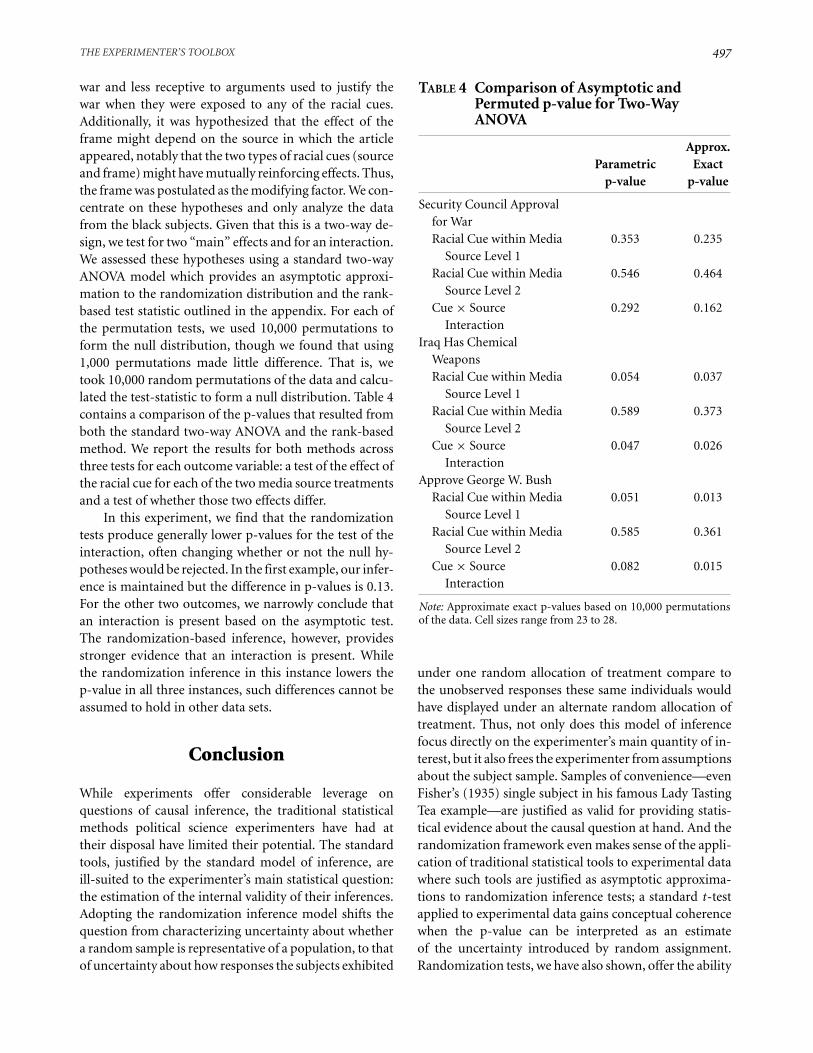
war and less receptive to arguments used to justify thewar when they were exposed to any of the racial cues.Additionally, it was hypothesized that the effect of theframe might depend on the source in which the articleappeared, notably that the two types of racial cues (sourceand frame) might have mutually reinforcing effects. Thus,the frame was postulated as the modifying factor. We con-centrate on these hypotheses and only analyze the datafrom the black subjects. Given that this is a two-way de-sign, we test for two “main” effects and for an interaction.We assessed these hypotheses using a standard two-wayANOVA model which provides an asymptotic approxi-mation to the randomization distribution and the rank-based test statistic outlined in the appendix. For each ofthe permutation tests, we used 10,000 permutations toform the null distribution, though we found that using1,000 permutations made little difference. That is, wetook 10,000 random permutations of the data and calcu-lated the test-statistic to form a null distribution. Table 4contains a comparison of the p-values that resulted fromboth the standard two-way ANOVA and the rank-basedmethod. We report the results for both methods acrossthree tests for each outcome variable: a test of the effect ofthe racial cue for each of the two media source treatmentsand a test of whether those two effects differ.

In this experiment, we find that the randomizationtests produce generally lower p-values for the test of theinteraction, often changing whether or not the null hy-potheses would be rejected. In the first example, our infer-ence is maintained but the difference in p-values is 0.13.For the other two outcomes, we narrowly conclude thatan interaction is present based on the asymptotic test.The randomization-based inference, however, providesstronger evidence that an interaction is present. Whilethe randomization inference in this instance lowers thep-value in all three instances, such differences cannot beassumed to hold in other data sets.

Conclusion

While experiments offer considerable leverage onquestions of causal inference, the traditional statisticalmethods political science experimenters have had attheir disposal have limited their potential. The standardtools, justified by the standard model of inference, areill-suited to the experimenter’s main statistical question:the estimation of the internal validity of their inferences.Adopting the randomization inference model shifts thequestion from characterizing uncertainty about whethera random sample is representative of a population, to thatof uncertainty about how responses the subjects exhibited

TABLE 4 Comparison of Asymptotic andPermuted p-value for Two-WayANOVA

Approx.Parametric Exact

p-value p-value

Security Council Approvalfor WarRacial Cue within Media

Source Level 10.353 0.235

Racial Cue within MediaSource Level 2

0.546 0.464

Cue × SourceInteraction

0.292 0.162

Iraq Has ChemicalWeaponsRacial Cue within Media



0.589 0.373


0.047 0.026

Approve George W. BushRacial Cue within Media



0.585 0.361


0.082 0.015

Note: Approximate exact p-values based on 10,000 permutationsof the data. Cell sizes range from 23 to 28.

under one random allocation of treatment compare tothe unobserved responses these same individuals wouldhave displayed under an alternate random allocation oftreatment. Thus, not only does this model of inferencefocus directly on the experimenter’s main quantity of in-terest, but it also frees the experimenter from assumptionsabout the subject sample. Samples of convenience—evenFisher’s (1935) single subject in his famous Lady TastingTea example—are justified as valid for providing statis-tical evidence about the causal question at hand. And therandomization framework even makes sense of the appli-cation of traditional statistical tools to experimental datawhere such tools are justified as asymptotic approxima-tions to randomization inference tests; a standard t-testapplied to experimental data gains conceptual coherencewhen the p-value can be interpreted as an estimateof the uncertainty introduced by random assignment.Randomization tests, we have also shown, offer the ability


to avoid parametric assumptions, confidence intervalsthat are informative about testing power, and a capacityto change substantive inferential conclusions.

The randomization inference framework can also beextended in many ways that we did not review here.Rosenbaum (2002a) outlines a method for covarianceadjustment that is fully integrated with randomizationtests and is easy to implement. Such covariate adjust-ment can be helpful for increasing the power of a test.There are also randomization tests for block designs andwithin-subjects experiments. Hansen and Bowers (2009)adapt the randomization framework to an experimentaldesign with clustering and noncompliance. Rosenbaum(2002b) uses randomization inference as a basis for sen-sitivity analysis in observational studies. As advances incomputing continue, randomization inference tools areincreasingly finding their way into common statisticalsoftware packages. Familiarity seems the only remainingimpediment to the integration of the randomization in-ference approach into the methodological toolkit of theexperimenter in political science.

References

Fisher, Ronald A. 1935. The Design of Experiments. London:Oliver and Boyd.

Fowler, James H., and Cindy D. Kam. 2007. “Beyond the Self:Social Identity, Altruism, and Political Participation.” Jour-nal of Politics 69(3): 813–27.

Freedman, David A. 2008a.“On Regression Adjustments in Ex-perimental Data.” Advances in Applied Mathematics 40(2):180–93.

Freedman, David A. 2008b. “On Regression Adjustments inExperiments with Several Treatments.” Annals of AppliedStatistics 2(1): 179–96.

Freedman, David A. 2008c. “Randomization Does Not JustifyLogistic Regression.” Statistical Science 23(2): 237–49.

Gelman, Andrew, and Jennifer Hill. 2006. Data Analysis UsingRegression and Multilevel/Hierarchical Models. Cambridge:Cambridge University Press.

Gill, Jeff. 1999. “The Insignificance of Null Hypothesis Signifi-cance Testing.” Political Research Quarterly 52(3): 647–74.

Hansen, Ben B., and Jake Bowers. 2008. “Covariate Balancein Simple, Stratified, and Clustered Comparative Studies.”Statistical Science 23(2): 219–36.

Hansen, Ben B., and Jake Bowers. 2009. “Attributing Effects to aClustered Randomized Get-Out-the-Vote Campaign.” Jour-nal of the American Statistical Association 104(487): 873–85.

Higgins, James J. 2003. Introduction to Modern NonparametricStatistics. Belmont, CA: Duxbury Press.

Ho, Daniel E., and Kosuke Imai. 2006. “Randomization Infer-ence with Natural Experiments: An Analysis of Ballot Effectsin the 2003 Election.” Journal of the American Statistical As-sociation 101(475): 888–900.

Hodges, J. L., and E. L. Lehmann. 1963. “Estimates of Loca-tion Based on Ranks.” The Annals of Mathematical Statistics34(2): 598–611.

Hoeffding, W. 1952. “The Large Sample Power of Tests Basedon Permutations of the Observations.” The Annals of Math-ematical Statistics 23(2): 169–92.

Hollander, Myles, and Douglas A. Wolfe. 1999. NonparametricStatistical Methods. 2nd ed. New York: John Wiley and Sons.

Imbens, Guido W., and Paul Rosenbaum. 2005. “Robust, Accu-rate Confidence Intervals with a Weak Instrument: Quarterof Birth and Education.” Journal of the Royal Statistical So-ciety Series A 168(1): 109–26.

Imbens, Guido W., and Donald B. Rubin. 2008. Causal Inferencein Statistics and the Medical and Social Sciences. Cambridge:Cambridge University Press.

Lehmann, E. L. 1975. Nonparametrics: Statistics Based on Ranks.San Francisco: Holden-Day.

Lehmann, E. L., and Joseph P. Romano. 2005. Testing StatisticalHypotheses. 3rd ed. New York: Springer.

Lin, Winston. 2010. “Agnostic Notes on Regression Adjustmentsto Experimental Data.” Unpublished manuscript. Universityof California, Berkeley.

Nelson, Thomas E., Rosalee Clawson, and Zoe M. Oxley. 1997.“Media Framing of a Civil Liberties Conflict and Its Effect onTolerance.” American Political Science Review 91(3): 567–83.

Neyman, Jerzy. 1923. “On the Application of Probability Theoryto Agricultural Experiments. Essay on Principles. Section 9.”Statistical Science 5(4): 465–72. Trans. Dorota M. Dabrowskaand Terence P. Speed (1990).

Rosenbaum, Paul R. 2001. “Effects Attributable to Treatment:Inference in Experiments and Observational Studies with aDiscrete Pivot.” Biometrika 88(1): 219–31.

Rosenbaum, Paul R. 2002a. “Covariance Adjustment in Ran-domized Experiments and Observational Studies.” Statisti-cal Science 17(3): 286–387.

Rosenbaum, Paul R. 2002b. Observational Studies. 2nd ed.New York: Springer.

Rosenbaum, Paul R. 2003. “Exact Confidence Intervals for Non-constant Effects by Inverting the Signed Rank Test.” TheAmerican Statistician 57(2): 132–38.

Rosenbaum, Paul R. 2007. “Interference between Units in Ran-domized Experiments.” Journal of the American StatisticalAssociation 102(477): 191–200.

Rubin, Donald B. 1986. “Which Ifs Have Causal Answers.” Jour-nal of the American Statistical Association 81(396): 961–62.

Sprent, Peter, and Nigel C. Smeeton. 2007. Applied Nonparamet-ric Statistical Methods. 4th ed. Boca Raton, FL: Chapman &Hall/CRC.

White, Ismail K. 2003. “Racial Perceptions of Support for theIraq War.” PhD dissertation. University of Michigan. Un-published data.

Supporting Information

Additional Supporting Information may be found in theonline version of this article:


Additional Information on Strengthening the Ex-perimenter’s Toolbox: Statistical Estimation of InternalValidity

Table A1: Asymptotic Relative Efficiency of RankSum Test and t-test

Please note: Wiley-Blackwell is not responsible for thecontent or functionality of any supporting materials sup-plied by the authors. Any queries (other than missingmaterial) should be directed to the corresponding authorfor the article.

strengthening the experimenters toolbox: statistical estimation of

Documents