stress projection, layerwise-equivalent,...
TRANSCRIPT

February 23, 2001 9:43 WSPC/156-IJCES 00003
International Journal of Computational Engineering ScienceVol. 1, No. 1 (2000) 91–138c© Imperial College Press
STRESS PROJECTION, LAYERWISE-EQUIVALENT,
FORMULATION FOR ACCURATE PREDICTIONS OF
TRANSVERSE STRESSES IN LAMINATED PLATES AND SHELLS
JAY Z. YUAN∗
Graduate Research Assistant, Department of Civil Engineering,The University of Akron, Akron, OH 44325, USA
ATEF F. SALEEB
Department of Civil Engineering, The University of Akron,Akron, OH 44325, USA
ATEF S. GENDY
Structural Engineering Department,Cairo University, Giza, Egypt
Received 16 August 1999Accepted 14 December 1999
A two-phase scheme for accurate predictions of interlaminar stresses in laminated plateand shell structures has been addressed in this study. A modified superconvergent patchrecovery (MSPR) technique has been utilized to obtain accurate nodal in-plane stresseswhich are subsequently used with the thickness integration of the three-dimensionalequilibrium equations to evaluate the transverse shear and normal stresses. Remarkably,the continuity of the resulting interlaminar stresses is automatically satisfied. Such atwo-phase scheme has been applied successfully to a simple smeared layer model (SLM),i.e., a low-order quadrilateral hybrid/mixed element (HMSH5). This simple procedureis found to be completely equivalent to the far more computationally expensive alterna-tive approaches, e.g., sophisticated layerwise approach, for flat geometry. A fairly largenumber of numerical examples have been solved and the results have shown that theproposed scheme is fairly reliable and computationally cost effective.
Keywords: Laminates; Transverse Stresses; Stress Recovery; Plates and Shells
1. Introduction
1.1. General
In a great variety of complex composite structural applications, plate and shell finite
element models are now almost invariably utilized in many phases of the analysis
∗Stress Engineering Services, Inc. 5380 Courseview Dr., Mason, OH 45040, USA.
91

February 23, 2001 9:43 WSPC/156-IJCES 00003
92 J. Z. Yuan, A. F. Saleeb & A. S. Gendy
and design processes. However, some of such complex applications, e.g., failure
studies and various damage mechanisms associated with composite materials, have
often posed great challenges for the analysts, in view of the fact that they are
beyond the capability of conventional shell element theory. Therefore, recent interest
has been focused on the theoretical developments and associated computational
algorithms for a number of refinements for the plate and shell models to be used in
the progressive failure analyses, design, and life predictions of composite laminated
structures. One of these refinements, which is addressed in this work, is associated
with the high gradients (or extreme discontinuity) of transverse shear strains in
highly-anisotropic composite laminates.
Being developed on the basis of hypotheses and assumptions, classical shell the-
ories and formulations are inherently approximate in nature. For instance, constant
transverse shear strains and zero normal stress in the thickness direction have been
often assumed. However, the transverse shear and normal stresses are usually non-
linear functions of thickness coordinates, due to dislike material in each of the layers.
By simply extending the ordinary shell formulations to laminated structures, only
the global responses; i.e., displacements, vibration frequencies, stress resultants,
and such, can be accurately captured. However, the local responses, such as inter-
laminar stresses, are only approximated in an integral sense. For instance, using
the kinematical assumptions of first-order, shear-deformable, shells, the resulting
interlaminar shear stresses become constant within each layer and the transverse
normal stress is implicitly taken to be zero through the whole thickness.
On the other hand, it is well known that laminated plate and shell structures
are more likely to fail due to “delamination”. Consequently, the determination of
“accurate” transverse shear stress variation through thickness, especially at lamina
interface and free edge, plays a vital role in the progressive failure study for such
structures.
To this end, since the classical single-layer shell theory is often inadequate to
determine the interlaminar stresses for the laminated plate and shell structures,
several refined laminate approaches have been proposed to date to extend the clas-
sical shell theory to account for such effects. As far as the shear deformations are
concerned, the “typical” kinematical assumptions for these extensions can be clas-
sified into several categories: (1) first-order (shear deformation) equivalent-single-
layer (FESL) approach; (2) higher-order (shear deformation) equivalent-single-layer
(HESL) approach; (3) layerwise approach. The spirit of these approaches is to re-
duce the three dimensional problem into a two-dimensional one, thereby reducing
the computational cost. A brief literature review of some of the research works
concerning these approaches is given in the sequel.
1.2. Literature review
Starting with the First-order (shear deformation) equivalent-single-layer (FESL)
approach, this approach extends the classical single-layer theory by accounting

February 23, 2001 9:43 WSPC/156-IJCES 00003
Transverse Stresses in Laminated Plates and Shells 93
for the varying layer thickness and material properties in an integral sense. For
many applications, the FESL approach provides a sufficiently accurate description
of the global laminate response (e.g., transverse deflection, fundamental vibration
frequency, critical buckling load, force and moment resultants, etc.). The main ad-
vantages of the FESL models are their inherent simplicity and low computational
cost due to the relatively small number of dependent variables that have to be
solved. However, the FESL models are often inadequate in determining the three-
dimensional field at the ply level. The major deficiency of the FESL models in
modeling composite laminates is that the accuracy of transverse stresses mainly
depends on the accuracy of corresponding in-plane stresses when the transverse
stresses are computed through stress equilibrium. For example, for a displacement-
based shell (plate) element, in order to get a linear distribution for transverse shear
stresses along the thickness direction (instead of constant distribution carried out
by constitutive equations), at least a linear distribution for in-plane stresses in mid-
surface is required. This means that one has to utilize quadratic or even higher-order
elements; e.g., 9-node or 16-node quadrilateral element, where the surface displace-
ment interpolations of which (i.e., second or higher order polynomials) may lead
to the requirements for linear distribution of the in-plane stresses. Actually, this
is one of the main motivations for using higher-order elements in early attempts;
e.g. Chaudhuri, (1986), Tocher and Hartz, (1967). However, these elements suffer
from the following major deficiencies: (1) computational expensiveness, (2) high
distortion sensitivity.
For the Higher-order (shear deformation) equivalent-single-layer (HESL)
approach, the transverse stresses can also be carried out through the constitutive
equations instead of using the equilibrium. This leads to a higher-order (shear de-
formation) equivalent-single-layer approach. In this approach, a higher-order kine-
matics is assumed in thickness direction in order to capture the complex shear
deformation of laminated structures. The varying layer thickness and material prop-
erties are still considered in an integral sense. Since a higher-order approximation is
made in shear deformation and transverse strains, more accurate transverse stresses
(compared with those of FESL) can be expected. However, this approach has its
own major deficiencies: (1) the variables associated with the higher-order terms
have no physical meaning, (2) complex derivation leads to implementation difficul-
ties, (3) almost inextendable to the non-linear plasticity analysis, (4) the continuity
of interlaminar stresses is still not satisfied, and (5) computationally expensive.
Both FESL and HESL approaches mentioned above belong to the so-called
“smeared layer model” (SLM), because in such a model the varying layer thickness
and material properties are only considered in an integral sense. On the other
hand, one can also consider each layer (or layer group) individually. This leads to
the so-called “discrete layer model” (DLM). The discrete layer model widely used in
current literature is the layerwise constant strain approach, layerwise approach in
short. In such approach, the transverse strains are discontinuous across the interface
of the layers, which leaves a room to satisfy the interlaminar continuity of transverse

February 23, 2001 9:43 WSPC/156-IJCES 00003
94 J. Z. Yuan, A. F. Saleeb & A. S. Gendy
shear stresses. Such a continuity condition is often enforced through the satisfaction
of equilibrium equations along the thickness directions. Unlike the smeared layer
models, the layerwise approach accounts for each layer individually which leads to
accurate transverse shear stresses. However, corresponding computational expense
is also greatly increased. Basically, an assembly process is required to form the
element, or laminate, stiffness from the individual layer stiffness. As pointed out
by Spilker, Jakobs and Engelmann (1985) the number of degree-of-freedom grows
rapidly as the number of layers increases and computer core storage may limit the
number of layers allowed. This has motivated a large number of efforts to modify
the “direct” layerwise approach, aiming at the reduction in computational expense;
e.g. see Averill and Reddy (1992), Reddy (1993), Barbero (1992) and Zinno and
Barbero (1994) among many others.
Because of their high computational cost, the layerwise and HESL approaches
are often applied in combination with less expensive schemes, such as FESL ap-
proach to reduce the total computational cost. In other words, since accurate trans-
verse shear stresses are often required only in a certain small region, the rest of the
problem domain can be analyzed by using less expensive approaches. The global-
local analysis technique [Ochoa and Reddy, 1992] and hierarchic models [Babuska
et al., 1992] are motivated by such a consideration. The global-local analysis refers to
the combination of layerwise approach and FESL approach in a practical problem.
This technique can be considered as an h-version refinement topology. In this, the
refinement is made in the thickness direction instead of in the in-plane dimensions.
However, transition elements or equivalent computational procedures are needed
to pass the variables from the global analysis to the local one. This often leads to
implementation complexity and application inconvenience. Parallel to the global-
local analysis, the hierarchic models have been proposed by Babuska and coworkers
(1992). The hierarchic models refer to the combination of HESL and FESL ap-
proaches. The hierarchic sequence of the models is classified based on the degree of
equilibrium equations satisfied by the model. Different from the global-local analy-
sis technique, for hierarchic models, in a particular application, the accuracy of the
region of most interest can be increased by choosing a high order model locally while
the whole mesh remains unchanged; thus transition elements are not needed. It is
specifically efficient for accounting for the boundary layer effects. This technique can
be considered as a p-version refinement topology. Again, in this case the refinement
is made in the thickness direction. However, this approach is somewhat restricted in
applications because some assumptions must be made to simplify the complicated
manual derivation; e.g., only a laminated strip is discussed in [Babuska et al., 1992].
1.3. Objective and outline
Based on the preceding literature review in the area of handling laminated struc-
tures by the two-dimensional analysis, it can be concluded that most, if not all, of
the proposed approaches are either too simple to capture the intrinsic behavior of

February 23, 2001 9:43 WSPC/156-IJCES 00003
Transverse Stresses in Laminated Plates and Shells 95
transverse shear and normal stresses at lamina interfaces and free edges (FESL)
or too expensive and/or restrictive to be applied independently (HESL, layerwise,
global-local technique and hierarchic models). The present effort focuses on the de-
velopment of a low-order quadrilateral model and layerwise equivalent finite element
approach for general laminate shell applications. As demonstrated in the applica-
tions section, the resulting model is not only computationally economical but also
capable of accurately predicting stress components at the layer level.
To this end, we are introducing a two-phase hierarchical approach to accurately
predict interlaminar stresses corresponding to localized regions of high transverse
strain fields across the thickness in laminates. In its first phase, a modified su-
per convergent patch recovery (MSPR) technique is utilized to obtain accurate,
through the thickness, distributions of nodal in-plane stresses. These are subse-
quently utilized, in the second phase, together with the thickness integration of the
three-dimensional (3D) equilibrium equations to evaluate the transverse shear and
normal stresses.
In summary, in our proposed methodology, the classical FESL approach has
been extended by exploiting an appropriate stress projection, i.e., modified super-
convergent patch recovery technique (MSPR), as post-processing. Since the super-
convergent property of in-plane stresses can be obtained by this MSPR technique,
the corresponding transverse stress can be carried out accurately by satisfying the
equilibrium through-the-thickness pointwise. The mathematical derivations prove
that such a simple approach is actually equivalent (in terms of the good quality and
accuracy of results) to the more sophisticated, layerwise, approach for the case of
plate structures. The proposed scheme is readily extendible to include both geomet-
ric and material nonlinear effects (since such an extension is made outside the main
finite element’s formulation). In addition, like the underlying FESL approach, it is
also applicable to thin as well as to moderately thick laminate plate- and shell-type
structures. The present methodology has been applied to a fairly large number of
sample problems using the modified HMSH5 quadrilateral element [Saleeb et al.,
1987, 1990] as a vehicle for analysis to assess its efficiency, accuracy and robustness.
2. Modified Superconvergent Patch Recovery (MSPR) Procedure
In this section, the Superconvergent Patch Recovery (SPR) scheme proposed by
Zienkiewicz and Zhu (1992 and 1994) is extended to the present Modified Super-
convergent Patch Recovery (MSPR). The major modification is that an isopara-
metric coordinates system is utilized in MSPR to perform the least square fitting.
Thus, MSPR can be applied to general curved shell applications, and the resulting
geometrical interpolatory scheme is thus completely devoid of any singularity in
general geometries of element patches, see also Sec. 7.1.2.
In the MSPR procedure, the nodal in-plane stress vector σ∗ is assumed to be a
polynomial expansion. Such a polynomial is valid over an element patch surrounding
the particular assembly node considered (see Fig. 1); where the element patch has

February 23, 2001 9:43 WSPC/156-IJCES 00003
96 J. Z. Yuan, A. F. Saleeb & A. S. Gendy
Fig. 1. A typical patch of HMSH5.
nine nodes defining its geometry of such a patch as shown in Fig. 1. The polynomial
expansion may be expressed for each ith component of σ∗, as
σ∗i = P a (1)
where P = [1, r, s, rs] and a is a set of unknown parameters. The polynomial
expansion in Eq. (1) is expressed in the isoparametric coordinate defined by the 9
nodes of the patch, that is
x(r, s, t) =
9∑k=1
Nkxk +t
2
9∑k=1
hkNkef(k)3 (2)
where x = (x, y, z) are the Cartesian coordinates of a point in the patch; xk is the
position vector of nodal point k on the reference surface; ef(k)3 are the components of
a unit vector emanating from node k in the fiber direction; hk is the fiber dimension
of shell thickness at node k; and Nk is the “familiar” two-dimensional Lagrangian
shape function in terms of (r, s) associated with node k.
The determination of the unknown parameters a of the expansion given in
Eq. (1) is best made by ensuring a least square fit of this to the set of superconvergent
(or at least high accuracy) sampling points existing in the patch considered, if such
points are available. Since the MSPR procedure is performed in an isoparametric
surface with constant thickness-coordinate t, it can be omitted in the following for
convenience. To perform the least square fit we minimize the following function:
F (a) =
4∑i=1
(σh(ri, si)− σ∗(r, s)
)2=
4∑i=1
(σh(ri, si)−P(r, s)a
)2(3)
where (ri, si) are the natural coordinates of a group of “optimal” sampling points,
σh(ri, si) are the components of the in-plane stress vectors calculated directly from
finite element analysis (where their components are resolved in the local coordi-
nates at centroid of each corresponding element). In addition to the basic form
of error terms in Eq. (3) above, several other modifications and enhancements
to the original SPR strategy have also been proposed in the literature; e.g., to

February 23, 2001 9:43 WSPC/156-IJCES 00003
Transverse Stresses in Laminated Plates and Shells 97
include tractions/displacement boundary terms, or to append additional, penatly-
like, curvature-control functions to achieve higher-order degrees of smoothing for
the recovered stress fields (Tessler, Riggs, and Macy, 1994).
The minimization condition of F (a) implies that the unknown parameter vector
a has to satisfy
4∑i=1
PT(ri, si)P(ri, si)a =
4∑i=1
PT(ri, si)σh(ri, si) . (4)
This can be solved in matrix form as
a = A−1 b (5)
where
A =
4∑i=1
PT(ri, si)P(ri, si) and b =
4∑i=1
PT(ri, si)σh(ri, si) . (6)
For boundary nodes, the patches are assembled and solved in the way shown in
Figs. 2 and 3, i.e., we simply recover the stresses at the edge and corner nodes for
the corresponding patch associated with the adjacent interior nodes. In addition to
its simplicity, this boundary treatment will also maintain the important property of
superconvergence for the present linear quadrilateral element. This latter property
has been confirmed in all our numerical experiments performed to date. The same
property was also demonstrated for the plane-stress/strain cases in Zienkiewicz and
Zhu (1992, 1994). See also related discussions in the later Sec. 7.1.2. Furthermore, we
have also performed a number of limited numerical experiments utilizing alternate
recovery schemes in which additional conditions are included; e.g., traction-free
conditions at free edges, specified boundary displacements, etc., but the results did
not exhibit any significant improvements. Extended work and results of this type
will be reserved for a future publication.
As in the SPR procedure precisely the same matrix A is needed for the solution
of each component of σ∗ and hence only a single evaluation of such a matrix is
necessary. Since only four equations need to be solved for each patch in the case
Fig. 2. Boundary nodal recovery (corner node).

February 23, 2001 9:43 WSPC/156-IJCES 00003
98 J. Z. Yuan, A. F. Saleeb & A. S. Gendy
Fig. 3. Boundary nodal recovery (edge node).
of the present linear quadrilateral element we considered, the whole procedure is
quite inexpensive. On the other hand, because the sample points are located in the
centroid of each element and the stress functions in Eq. (1) are complete bilinear
polynomials, the superconvergent property of recovered nodal stresses (both interior
and boundary) still remains.
It is also worthwhile repeating that the singularity problem in SPR is completely
eliminated here (see Sec. 7.1.2). This singularity problem, which is also noticed
by Zienkiewicz and Zhu (1994) is that the determinate of the matrix A defined
in Eq. (5) is not always nonzero if the recovery scheme is formed in the global
coordinate described in the SPR. Thus, the SPR will not be applicable for some
geometrical patch alignments (see Sec. 7.1.2).
The patch recovery technique provides not only the superconvergence of the in-
plane nodal stresses themselves but also their accurate (first) derivatives from the
bilinear polynomial assumptions on each patch. Therefore, the following step of ap-
plying 3D stress equilibrium equations becomes more straightforward. In addition,
applying the patch recovery technique to the hybrid/mixed formulation provides
the same superconvergent rate to all three in-plane stress components rather than
being treated differently in their original polynomial assumptions, i.e., linear as-
sumption for σx and σy, constant assumption for τxy; see references Saleeb et al.,
(1987, 1988, 1990). This equal importance of the rate of convergence of all three
recovered in-plane stresses benefits the following procedure of applying the equilib-
rium equations. In particular, the above three in-plane stresses have equal position
in equilibrium equations (see Sec. 3) and the final solutions for recovering inter-
laminar stresses can be disturbed by any lack of accuracy in any of the in-plane
components.
3. Transverse Stresses via Equilibrium Equations
The elasticity equilibrium equations for the ith layer of a multi-layered laminate
have the following general form
Divσ + ρb = 0 . (7)

February 23, 2001 9:43 WSPC/156-IJCES 00003
Transverse Stresses in Laminated Plates and Shells 99
Here, σ denotes the symmetric Cauchy stress tensor; and ρb are the body forces
(which will be neglected in the following equations), and Div is the divergence
operator.
The three differential equations of equilibrium, i.e, Eq. (7), give three relations,
namely,
∂τxz
∂z= −
(∂σx
∂x+∂τxy
∂y
)(8a)
∂τyz
∂z= −
(∂τxy
∂x+∂σy
∂y
)(8b)
and
∂2σz
∂z2=∂2σx
∂x2+∂2σy
∂y2+ 2
∂2τxy
∂x∂y(8c)
from which the transverse stresses τxz, τyz and σz can be evaluated through integra-
tion with respect to the laminate thickness z. As described previously, the in-plane
normal stresses σx and σy and the in-plane shear stress τxy utilized in Eq. (8) are
obtained by the modified superconvergent patch recovery scheme.
The final τxz and τyz for the ith layer whose z-dimension ranges between hi−1
at the bottom to hi at the top, of an N -layer laminated shell can be integrated
through the thickness either from the bottom surface, i.e.,
iτxz(z) = −i−1∑k=1
∫ hk
hk−1
(∂iσx
∂x+∂iτxy
∂y
)dζ −
∫ z
hi−1
(∂iσx
∂x+∂iτxy
∂y
)dζ (9a)
iτyz(z) = −i−1∑k=1
∫ hk
hk−1
(∂iσy
∂y+∂iτxy
∂x
)dζ −
∫ z
hi−1
(∂iσy
∂y+∂iτxy
∂x
)dζ (9b)
or, from the top surface, i.e.,
iτxz(z) = −N∑
k=i+1
∫ hk−1
hk
(∂iσx
∂x+∂iτxy
∂y
)dζ −
∫ z
hi
(∂iσx
∂x+∂iτxy
∂y
)dζ (9c)
iτyz(z) = −N∑
k=i+1
∫ hk−1
hk
(∂iσy
∂y+∂iτxy
∂x
)dζ −
∫ z
hi
(∂iσy
∂y+∂iτxy
∂x
)dζ . (9d)
Note that since ∂x, ∂y and τxy are linearly distributed along the thickness in each
layer, the transverse shear stresses computed from Eqs. (9) are quadratic variations
through the thickness.
February 23, 2001 9:43 WSPC/156-IJCES 00003
100 J. Z. Yuan, A. F. Saleeb & A. S. Gendy
4. Continuity of Interlaminar Transverse Shear Stresses
Integrating either Eqs. (9a) and (9b), starting from the bottom surface (or Eqs.
(9c) and (9d)), starting from the top surface) could, in principle, lead to different
values for transverse shear stresses at a given location, i.e., a nonunique solution
for transverse shear stresses can be obtained. However, it will be proved next that
the interlaminar continuity of the transverse shear stresses is actually automatically
satisfied utilizing the proposed approach.
In the regular finite element formulation, the equilibrium through the thickness
is satisfied in an integral sense, that is,∫ hN
h0
(∂σx
∂x+∂τxy
∂y+∂τxz
∂z
)dz = 0 (10a)
∫ hN
h0
(∂τxy
∂x+∂σy
∂y+∂τyz
∂z
)dz = 0 (10b)
In addition, the transverse shear stresses are usually known at the top and
bottom surfaces of the laminate (e.g., zero for no surface tractions), i.e.,
τxz(hN ) = τxz(h0) = 0 (11a)
τyz(hN ) = τyz(h0) = 0 (11b)
Substituting from Eqs. (11a) and (11b) into Eqs. (10a) and (10b) respectively,
and noting that in the modified superconvergent recovery technique the in-plane
stress components satisfy the in-plane equilibrium equations in each layer, i.e.,
Eqs. (8a), (8b) and (10a) can be integrated through the thickness utilizing the
proposed procedure as
N∑k=1
∫ hk
hk−1
(∂σx
∂x+∂τxy
∂y
)dζ = 0 . (12a)
This can be expressed as (after exchanging the integration limits)
i∑k=1
∫ hk
hk−1
(∂σx
∂x+∂τxy
∂y
)dζ =
N∑k=i+1
∫ hk−1
hk
(∂σx
∂x+∂τxy
∂y
)dζ . (13a)
Similarly, Eq. (10b) can be expressed as
i∑k=1
∫ hk
hk−1
(∂τxy
∂x+∂σy
∂y
)dζ =
N∑k=i+1
∫ hk−1
hk
(∂τxy
∂x+∂σy
∂y
)dζ . (13b)
From Eqs. (13a), (13b) and Eqs. (9a) and (9b), one concludes that the interlaminar
shear stresses are thus continuous across each layer, i.e., the continuity of interlam-
inar shear stress is satisfied.

February 23, 2001 9:43 WSPC/156-IJCES 00003
Transverse Stresses in Laminated Plates and Shells 101
Fig. 4. A typical layer i and its interfaces.
5. Equivalent Layerwise Linear Kinematics
We now focus on a typical layer (Fig. 4). The stress resultants of such typical layer
i can be expressed according to Fig. 4 as
inα =
∫ jh2
− ih2σ eαdζ ,
imα =
∫ jh2
− ih2
(ix− ix0
)⊗ σ eαdζ (14)
where n and m are the resultant vectors of normal forces and bending moments,
respectively; σ eα is Cauchy stress vector on the plane whose normal is defined
by eα; α = 1, 2 for plane x-z and y-z, respectively; and, the symbol (⊗) indicates
cross product of vectors. Integrate equilibrium equations, i.e., Eq. (7), through the
thickness of the layer i yields the following set of static field equations:
inα∣∣∣α
+ iq− i−1q = 0 (15a)
imα∣∣∣α
+ ix0,α × inα +ih
2ia3 ×
(iq + i−1q
)= 0 (15b)
and boundary conditions,
ναinα = 0 , να
imα = 0 on ∂Ωσ
iu = iu , ia3 = ia3 on ∂Ωu(15c)
where (.)α∣∣α
is the covariant derivative of the quantity (indicated in Eq. (15b)) with
respect to lamina direction α; i−1q and iq are the traction force vectors, and the
superscript i− 1 and i refer to the lower and upper surfaces of layer i, respectively;
να (α = 1, 2) are the components of the normal vector of boundary Ωσ; and iakis the orthonormal basis system describing the deformed cross-section of layer i.

February 23, 2001 9:43 WSPC/156-IJCES 00003
102 J. Z. Yuan, A. F. Saleeb & A. S. Gendy
Again, due to the effect of transverse shear strains, the “director” vector ia3 is
generally not normal to the current middle surface of the ith layer.
An equivalent discrete weak formulation can be obtained by weighting the field
equations with test functions δix0 and δiw, i.e.,∫Ω
N∑i=1
[inα∣∣α
+ iq− i−1q]· δix0
dΩ
+
∫Ω
N∑i=1
[imα
∣∣α
+ ix0,α × inα +ih
2ia3 ×
(iq + i−1q
)]· δiw
dΩ
+
∫∂Ωσ
N∑i=1
(να
inα)· δix0 +
(να
imα)· δiw
d∂Ω = 0 (16)
where δiw is the axial vector following the variation of the basis system iak in the
current configuration, i.e.,
δiak = δiw× iak . (17)
Assuming that the axial displacement is linearly distributed along the thickness
within each layer, i.e.,
δix = δix0 + iζδia3 −ih
2≤ ζ ≤
ih
2(18)
where the variable δia3 in general is different for different layers, our objective is
to prove that the axial displacement is actually continuous across the interface of
the layers. To this end, it is known that the contribution of the interlaminar stressiq (i = 0, 1, . . . , N) within the variational formulation has to vanish, i.e.,
0 =
∫Ω
N∑i=1
[(iq− i−1q
)· δix0 +
ih
2ia3 ×
(iq + i−1q
)· δiw
]dΩ
=
∫Ω
N∑i=1
[iq ·
(δix0 +
ih
2δia3
)− i−1q ·
(δix0 +
ih
2δia3
)]dΩ . (19)
Since 0q and Nq are equal to zero, Eq. (19) can be rewritten (after employing
Eq. (18)) as follows:
=
∫Ω
N−1∑i=1
[iq ·
(δix0 +
ih
2δia3
)]−
N∑i=2
[i−1q ·
(δix0 −
ih
2δia3
)]dΩ
=
∫Ω
N−1∑i=1
[iq ·
(δix0 +
ih
2δia3
)]−N−1∑i=1
[iq ·
(δi+1x0 −
i+1h
2δi+1a3
)]dΩ
=
∫Ω
N−1∑i=1
iq ·
[(δix0 +
ih
2δia3
)−(δi+1x0 −
i+1h
2δi+1a3
)]dΩ . (20)

February 23, 2001 9:43 WSPC/156-IJCES 00003
Transverse Stresses in Laminated Plates and Shells 103
Thus, one finally gets
δix0 +ih
2δia3 = δi+1x0 −
i+1h
2δi+1a3 for i = 1, 2, . . . , N − 1 , (21)
that is, the continuity of interlaminar kinematics condition is obtained. This shows
equivalency in the sense of layerwise-constant transverse shear strain distribution
as with more sophisticated layerwise kinematics models Babuska et al., (1992),
Kant and Manjunatha, (1988, 1994), Reddy, (1993), Ren, (1986,1987), Seide and
Chaudhuri, (1987), Sciuva, (1987), Spilker et al., (1977, 1985) among several others.
Remark 1:
The mathematical arguments and proofs given above for interlaminar-stress-
continuity and layerwise constant strain equivalency are based on the requirement
that in-plane equilibrium satisfaction is approached. For flat geometry, this fact is
met simply because the superconvergency of in-plane stresses is achieved “exactly”.
For general spatially-curved shells, however, since the element patches can not fully
match the curved geometry, the superconvergency of in-plane stresses is only ap-
proached asymptotically through mesh refinement.
Remark 2:
As a corollary to the above remark, the asymptotic property of superconvergence
must also carry over to the interpretation of all the “equivalency” results given.
That is, this latter equivalency does not imply “equality” or “identity” in the strict
mathematical sense, but rather it indicates comparable accuracy and good quality
of the results. In particular, in practice, where relatively coarse meshes are utilized,
results from the present approach and those from alternatives based on truly layer-
wise formulations, will be different in their details. For example, direct evaluation
of interlaminar stresses (i.e., from constitutive equations) will not guarantee their
continuity. Furthermore, the degree of approximations (in-plane discretizations) of
the underlying plate/shell formulations (e.g. 4-noded, 9-noded, etc.) will also impact
the accuracy of respective results in any of these latter schemes.
Remark 3:
Considering the important practical situations involving free edges in laminated
plate/shell problems, additional important factors will also come to play. Here, the
characteristic sharp variations (singularities, localizations, etc.) in the gradients of
the in-plane stress fields must be captured, through local in-plane mesh refinement
near these edges, before ensuring the prerequisite (close) satisfaction of equilibrium
conditions in the present approach (of course, accuracy considerations demand sim-
ilar mesh refinements in other alternative approaches, irrespective of the degree of
approximations utilized in the thickness direction). Although not specifically ad-
dressed here, our numerical experiments with such problems have yielded results

February 23, 2001 9:43 WSPC/156-IJCES 00003
104 J. Z. Yuan, A. F. Saleeb & A. S. Gendy
that are quite positive. In particular, the recovery scheme utilized was found very
effective in capturing nearly-singular variations in stresses at edges, and an im-
portant case to the point is included in Sec. 7.4 for a strongly-anisotropic beam
problem.
6. Interlaminar Transverse Normal Stress
The transverse normal stress can be obtained by integrating the second-order dif-
ferential equation, i.e., Eq. (8c), twice. Two constants of integration result for each
layer. Two described stress conditions on the top and bottom surfaces plus conti-
nuity conditions at layer interface are insufficient to define all those constants of
integration for laminate problems. However, in a thin plate/shell problem, such a
transverse normal stress can be approximated as
iσz(z) =
∫ih
∫ih
(∂2σx
∂x2+∂2σy
∂y2+∂2τxy
∂x∂y
)dzdz︸ ︷︷ ︸
Compute locally
+ C3z + C4︸ ︷︷ ︸Compute globally
(22)
where the constants C3 and C4 are obtained from the known values of σz at
z = ±H/2 (H is the total thickness of the laminate). It is worthwhile to men-
tion that unlike in Eqs. (9a) and (9b), the second derivatives of the in-plane stress
components appear in Eq. (22). Because of the bilinear assumption in Eq. (1), only
a constant results for the terms between the brackets in Eq. (22). Thus the trans-
verse normal stress is expected to be less accurate than the corresponding transverse
shear stresses; (e.g., a bi-quadratic polynomial assumption has to be introduced to
get the same or comparable accuracy). In addition, such a normal stress can also
be discontinuous across the interface of the layers. In fact, the continuity of inter-
laminar transverse normal stress can not be generally satisfied until the equality of
the derivatives of axial displacements at interfaces are enforced.
7. Numerical Examples
The solution scheme developed above has been implemented in conjunction with
a 5-noded mixed shell linear-quadrilateral element, designated here as HMSH5,
(i.e., with independently assumed displacement/rotation and strain fields within
the element) for the analysis of composite laminates; e.g. see Saleeb et al., (1987 &
1990). In this, the mixed element possesses a multi-layered capability (e.g., see Wilt,
Saleeb and Chang (1990) in which each layer contains (3×3) integration points in
the lamina plane in addition to two integration points in the thickness direction.
All numerical results reported here have been obtained using this model. These are
selected to demonstrate the capabilities, as well as various aspects, of the proposed
scheme; e.g., robustness, accuracy and computational efficiency. In particular, an
emphasis is placed on laminated plate/shell problems with relatively small thick-
ness aspect ratios (i.e., moderate and thick cases) where greater effects of trans-
verse shear deformations exist, together with complex distributions of interlaminar

February 23, 2001 9:43 WSPC/156-IJCES 00003
Transverse Stresses in Laminated Plates and Shells 105
stresses. However, for completeness, we have also included the results of a compos-
ite shell problem with a range of thicknesses (i.e., from thick to thin regimes). In
these numerical simulations, comparisons with available “exact” solutions as well
as other independent numerical schemes are also presented.
7.1. Convergence of nodal in-plane stresses obtained by MSPR
7.1.1. A square plate subjected to specified displacement field
A square plate with unit length is subjected to a specified displacement field as
u(x, y) = x(1− x)y(1− y)(1 + 2x+ 7y) (23)
where the origin of the x- and y-axes is located at the bottom left corner of this
plate, i.e., x and y range between 0 and 1. The displacement field u(x, y) vanish
along the plate boundary. The local error of the recovery stress σx is examined at a
nodal point with coordinates of (0.25, 0.25) where the exact solution has the values
of σx = 0.375. Uniform subdivisions 4×4, 8×8 and 16×16 meshes are used in the
finite element analysis. The results of σx obtained using the proposed scheme are
listed in Table 1 for different mesh size. The error of stress obtained from the MSPR
scheme is depicted in Fig. 5. As shown from this figure, the theoretically expected
superconvergent rate of 2 is reached here.
Fig. 5. Rate of convergence of error in stresses σx of present HMSH5 at the point (0.25, 0.25).

February 23, 2001 9:43 WSPC/156-IJCES 00003
106 J. Z. Yuan, A. F. Saleeb & A. S. Gendy
Table 1. σx of present HMSH5
evaluated at the point (0.25, 0.25).
mesh σx
4×4 0.3488×8 0.368
16×16 0.373Exact solution of σx 0.375
Fig. 6. Infinite plate with a central circular hole subjected to unidirectional tensile loads and theportion of the infinite plate analyzed.
7.1.2. Infinite plate with central circular hole
The problem considered here is a portion of an infinite plate with a central circular
hole subjected to a unidirectional tensile stress equal to unity as shown in Fig. 6.
Plane strain conditions are assumed with a Poisson’s ratio ν = 0.3 and Young’s
modulus E = 1000. A small portion of the plate near the hole is considered for
analysis. By making use of symmetry, only a quarter of such a portion is analyzed.
The boundary conditions are prescribed such that symmetry conditions are imposed
on edges AB and ED; and the plate is loaded by tractions given by an analytic

February 23, 2001 9:43 WSPC/156-IJCES 00003
Transverse Stresses in Laminated Plates and Shells 107
solution on edges BC and DC. Such tractions are expressed as
σx = 1− 1
r2
(3
2cos 2θ + cos 4θ
)+
3
2r4cos 4θ
σy = − 1
r2
(1
2cos 2θ − cos 4θ
)− 3
2r4cos 4θ (24)
τxy = − 1
r2
(1
2sin 2θ + sin 4θ
)+
3
2r4sin 4θ
where (r, θ) are the usual polar coordinates.
Three mesh sizes are used for the analysis, i.e., (12×6), (24×12) and (36×18).
The recovered stresses are examined at the nodal point (1.5, 450) where the exact so-
lution has the values of σx = 1.1481481, σy = −0.14814810 and τxy = −0.22222229.
Results from the finite elements are listed in Table 2 along with those from the an-
alytical solution. The errors in stresses are also depicted in Fig. 7 for different mesh
size. Again the numerical results show that the superconvergent property is fully
preserved in the proposed MSPR scheme.
Fig. 7. Convergence of the recovered in-plane stresses at the point (1.5, 450).

February 23, 2001 9:43 WSPC/156-IJCES 00003
108 J. Z. Yuan, A. F. Saleeb & A. S. Gendy
Table 2. In-plane stresses of present HMSH5 evaluated at the
point (1.5, 450).
mesh σx σy τxy
1 1.03843 −0.0371982 −0.2421572 1.09170 −0.0967173 −0.2280293 1.15910 −0.1542700 −0.225927
Exact solution 1.1481481 −0.1481481 −0.22222229
Remark 4:
It is of interest to note the patch surrounding the point (1.5, 450) (see Fig. 8). If the
patch recovery scheme is formed in the global coordinates, the matrix P in Eq. (1)
takes the following form
P =
1 a b ab
1 b a ab
1 c d cd
1 d c cd
. (25)
It is easy to verify that matrix P is singular and thus matrix A is also singular
(see Eq. (6)), which leads to non-unique solutions of the unknown parameters a.
However, if the original axes are rotated by an angle of 450 and the SPR is performed
in such a new coordinate system (x′, y′) (see Fig. 8), the matrix P becomes:
P =
1 a′ b′ a′b′
1 a′ −b′ −a′b′1 c′ d′ c′d′
1 c′ −d′ −c′d′
. (26)
This matrix P is non-singular unless a′ = c′. Such a singularity-free treat-
ment of rotating the axes is particularly important for most general cases involving
shells curved in space. Here, we completely by-pass the above singularity problem
and adopt surface-(lamina)-based components for the physical stresses in the shell
elements (see details in Saleeb et al. (1987 & 1990), with polynomial expansions in
terms of the natural/isoparametric coordinates, in Eqs. 1 and 26, when performing
the patch recovery scheme.
7.2. Accuracy and efficiency of the projection-layerwise-equivalent
approach
7.2.1. Cross-ply plates
Numerical results of the improved stress predictions by the present approach
for a group of cross-ply plates are presented in this section. The three-dimensional

February 23, 2001 9:43 WSPC/156-IJCES 00003
Transverse Stresses in Laminated Plates and Shells 109
(a) A patch leads to singularity of matrix A.
(b) The patch in the new co-ordinate system.
Fig. 8. Alternative coordinates for singularity-free patch recovery.
elasticity solutions of Pagano, (1970) for simply supported rectangular plates un-
der sinusoidal loading are used to assess the accuracy and reliability of the present
approach for different span to thickness ratios (a/h). In addition, results from two
different sophisticated layerwise approaches, by Reddy, (1993), Ren, (1987) as well
as one higher-order approach by Kant and Pandya, (1988) are also included for
comparison. The following four laminated plate problems are investigated: (1) Two
layers (0/90) square (b = a) laminate; (2) Three layers (0/90/0) square (b = a) lam-
inate; (3) Three layers (0/90/0) rectangular (b = 3a) laminate; and (4) Four layers
(0/90/90/0) square (b = a) laminate. The four problems are subjected transverse
loading defined as
q = q0 sinπx
asin
πy
b. (27)

February 23, 2001 9:43 WSPC/156-IJCES 00003
110 J. Z. Yuan, A. F. Saleeb & A. S. Gendy
The material coefficients for each layer are
EL = 25× 106 Et = 106
GLT = 0.5× 10⁶ GTT = 0.2× 10⁶
VLT = VTT = 0.25
(28)
where the subscripts L and T signify the parallel and transverse directions, respec-
tively, to the fiber. The following normalized quantities are defined with respect to
the data
(σx, σy, τxy
)=(σx, σy, τxy
)/(q0S
2)(
τyz, τxz)
=(τyz, τxz
)/(q0S)
σz = σz/q0
S = a/h z = z/h .
(29)
By making use of symmetry conditions, only a quarter of a plate has been used
for the analysis in which a mesh of 8×8 HMSH5 elements is utilized. Comparisons
of the stresses obtained using the MSPR approach with those provided either by
analytical solutions or numerical simulations, e.g., layerwise approach, are given in
Tables 3–8 for the four plate problems. Typical distributions for transverse stresses
over plate thickness are depicted in Figs. 9 and 10 for first plate problem and in
Figs. 11 and 12 for the third one. It is worthwhile to mention that the accurate
transverse stresses provided by the present scheme are based on the more accurate
in-plane stresses coming from the patch projection technique.
Remark 5:
All the transverse shear stresses reported are evaluated at the corner point of the
discretized model (due to symmetry considerations) for the four plate problems. The
worst approximation of the transverse stresses using the patch recovery scheme may
occur in such corner nodes since the in-plane stresses are extrapolated from a patch
similar to that shown in Fig. 3. In this case, the derivatives of these stresses with
respect to x and y are evaluated at the “dimensional limits” (i.e., x = a/2 and
y = b/2). To improve accuracy, the entire or half of the problem can be modeled
instead of its quarter. In this case the transverse stresses are still evaluated at the
boundaries, but they are away from the corners thus at least one of the derivatives
(with respect to x or y) is not in the dimension limit. Certainly, computational cost
will increase by such a solution. However, this is the case if there is no symmetrical
condition in the problem, such as the angle-ply plate examples illustrated in the
following section. It is also worthwhile to emphasize that the best approximation
would be inside element patch.

February 23, 2001 9:43 WSPC/156-IJCES 00003
Transverse Stresses in Laminated Plates and Shells 111
Table
3.
Str
esse
sin
square
lam
inate
pla
tew
itha/h
=4(0/90).
Pagano,
1970
Pre
sent
HM
SH
5
zσx
σy
τ yz
τ xz
τ xy
σx
σy
τ yz
τ xz
τ xy
( a 2,b 2,z
)( a 2
,b 2,z
)( a 2
,0,z)
( 0,b 2,z
)(0,0,z
)
−0.5
−0.7
807
−0.0
955
0.0
000
0.0
000
0.0
591
−0.7
328
−0.0
864
0.0
000
0.0
000
0.0
537
−0.4
−0.3
988
−0.0
734
0.0
423
0.1
976
0.0
427
−0.4
608
−0.0
729
0.0
388
0.1
957
0.0
430
−0.3
−0.1
437
−0.0
553
0.0
738
0.2
919
0.0
307
−0.1
887
−0.0
594
0.0
703
0.3
056
0.0
322
−0.2
0.0
598
−0.0
398
0.0
968
0.3
127
0.0
209
0.0
834
−0.0
460
0.0
944
0.3
297
0.0
215
−0.1
0.2
792
−0.0
258
0.1
122
0.2
659
0.0
117
0.3
554
−0.0
325
0.1
112
0.2
680
0.0
107
−0.0
0.5
872
−0.0
122
0.1
202
0.1
353
0.0
012
0.6
275
−0.0
190
0.1
206
0.1
206
0.0
000
+0.0
0.0
247
−0.6
307
0.1
202
0.1
353
0.0
012
0.0
190
−0.6
257
0.1
206
0.1
206
0.0
000
+0.1
0.0
372
−0.3
100
0.2
632
0.1
244
−0.0
089
0.0
325
−0.3
554
0.2
680
0.1
112
−0.0
107
+0.2
0.0
508
−0.0
789
0.3
188
0.1
063
−0.0
188
0.0
460
−0.0
834
0.3
297
0.0
944
−0.0
215
+0.3
0.0
667
0.1
387
0.3
027
0.0
807
−0.0
282
0.0
594
0.1
887
0.3
056
0.0
703
−0.0
322
+0.4
0.0
859
0.4
152
0.2
075
0.0
461
−0.0
410
0.0
729
0.4
608
0.1
957
0.0
388
−0.0
430
+0.5
0.1
098
0.8
417
0.0
000
0.0
000
−0.0
588
0.0
864
0.7
328
0.0
000
0.0
000
−0.0
537

February 23, 2001 9:43 WSPC/156-IJCES 00003
112 J. Z. Yuan, A. F. Saleeb & A. S. Gendy
Table 4. Transverse normal stress (σz) for simply supported laminate under sinu-soidal loading (a/h = 4) (0/90).
Transverse normal stress (σz)
Thickness HOST9(16N) [Kant, 1994] HMSH5 Elasticity [Pagano, 1970]
−0.5 0.000000 0.000000 0.000000
−0.4 0.072587 0.094968 0.078940
−0.3 0.175074 0.192091 0.250000
−0.2 0.289113 0.293080 0.460526
−0.1 0.399094 0.396046 0.671050
0.0 0.491027 0.500000 0.789474
+0.1 0.584600 0.603954 0.868421
+0.2 0.698580 0.706920 0.921053
+0.3 0.817625 0.807909 0.960526
+0.4 0.924730 0.905932 0.973684
+0.5 1.000000 1.000000 1.000000
Fig. 9. Variation of transverse shear stress (τxz) through the thickness of a simply supportedlaminate under sinusoidal loading (a/h = 4) (0/90).

February 23, 2001 9:43 WSPC/156-IJCES 00003
Transverse Stresses in Laminated Plates and Shells 113
Table 5. Stresses in square laminate plate with a/h = 10 (0/90).
Pagano, 1970 Present HMSH5
z σx σy τxy σx σy τxy(a
2,b
2, z
) (0,b
2, z
)(0, 0, z)
(a
2,b
2, z
) (0,b
2, z
)(0, 0, z)
−0.5 −0.730 0.000 0.0538 −0.733 0.000 0.0537
−0.4 −0.442 0.198 0.0422 −0.461 0.196 0.0430−0.3 −0.177 0.307 0.0314 −0.189 0.306 0.0322−0.2 0.077 0.331 0.0210 0.083 0.330 0.0215−0.1 0.335 0.271 0.0107 0.355 0.268 0.0107−0.0 0.610 0.125 0.0001 0.627 0.121 0.0000+0.0 0.020 0.125 0.0001 0.019 0.121 0.0000+0.1 0.033 0.115 −0.0104 0.033 0.111 −0.0107+0.2 0.046 0.098 −0.0207 0.046 0.094 −0.0215+0.3 0.060 0.073 −0.0311 0.060 0.070 −0.0322+0.4 0.074 0.041 −0.0420 0.073 0.039 −0.0430+0.5 0.089 0.000 −0.0536 0.087 0.000 −0.0537
Fig. 10. Variation of transverse shear stress (τyz) through the thickness of a simply supportedlaminate under sinusoidal loading (a/h = 4) (0/90).

February 23, 2001 9:43 WSPC/156-IJCES 00003
114 J. Z. Yuan, A. F. Saleeb & A. S. Gendy
Table 6. Normalized transverse shear stresses for simply-supported
square 0/90/0 plate with sinusoidal load.
S = a/h Source τyz(a/2, 0, 0) τxz(0, a/2, 0)
4 Elasticity [Pagano, 1970] 0.2170 0.2560
Present HMSH5 0.1947 0.3328
10 Elasticity [Pagano, 1970] 0.1228 0.3570
Present HMSH5 0.1095 0.3761
20 Elasticity [Pagano, 1970] 0.0938 0.3850
Present HMSH5 0.0889 0.3865
CLT 0.0823 0.3950
Fig. 11. Variation of the transverse shear stress (τxz) through thickness for 0/90/0 square plate(a/h = 4).

February 23, 2001 9:43 WSPC/156-IJCES 00003
Transverse Stresses in Laminated Plates and Shells 115
Table 7. Normalized transverse shear stresses for simply-supported rect-
angular (b = 3a) 0/90/0 plate with sinusoidal load.
S = a/h Source τyz(a/2, 0, 0) τxz(0, b/2, 0)
4 Elasticity [Pagano, 1970] 0.0334 0.351
Present HMSH5 0.0277 0.4195
10 Elasticity [Pagano, 1970] 0.0152 0.420
Present HMSH5 0.0175 0.4224
20 Elasticity [Pagano, 1970] 0.0119 0.4340
Present HMSH5 0.0113 0.4229
100 Elasticity [Pagano, 1970] 0.0108 0.439
Present HMSH5 0.0106 0.4230
CLT 0.0108 0.440
Fig. 12. Variation of the transverse shear stress (τyz) through thickness for 0/90/0 square plate(a/h = 4).

February 23, 2001 9:43 WSPC/156-IJCES 00003
116 J. Z. Yuan, A. F. Saleeb & A. S. Gendy
Table 8. Normalized transverse shear stresses for simply-supported
square 0/90/90/0 plate with sinusoidal load.
S = a/h Source τyz(a/2, 0, 0) τxz(0, a/2, 0)
4 Elasticity [Pagano, 1970] 0.292 0.270
Present HMSH5 0.2769 0.2654
10 Elasticity [Pagano, 1970] 0.1960 0.3010
Present HMSH5 0.1786 0.3143
20 Elasticity [Pagano, 1970] 0.1560 0.3280
Present HMSH5 0.1485 0.3290
100 Elasticity [Pagano, 1970] 0.1410 0.3370
Present HMSH5 0.1370 0.3350
Fig. 13. Variation of transverse shear stress (τyz) through the thickness of a simply supportedlaminate under sinusoidal loading (a/h = 10) (15/−15).

February 23, 2001 9:43 WSPC/156-IJCES 00003
Transverse Stresses in Laminated Plates and Shells 117
7.2.2. Angle-ply plates
Two square angle-ply laminated plates are considered: (1) two layers of equal thick-
ness with each ply alternately oriented at +150 and −150 to the x-y axes of the
plate; (2) eight layers of equal thickness with each ply alternately oriented at +450
and −450 to the x-y of the plate. The plates are simply supported by smooth pins
allowing tangential displacements along the boundaries and subjected to sinusoidal
load as the one given in Eq. (27). The lamina properties are similar to those given
in Eq. (28) for the first case, while they are defined by the following properties for
the second case
EL = 40× 106 Et = 106
GLT = 0.5× 10⁶ GTT = 0.6× 10⁶
VLT = VTT = 0.25 .
(30)
The whole plate has been analyzed using a 16×16 uniform mesh. The results for
these two particular problems are compared only with those provided by other
finite element solutions since there is no exact three-dimensional solution in a finite
domain for the angle-ply plate. The variation of transverse shear stress τyz through
the plate thickness of the first case is depicted in Fig. 13 along with that given
by Kant and Manjunatha, (1994). The variation of shear stress τxz is predicted in
Fig. 14 with that predicted by a higher order element as reported by Kant and
Pandya, (1988).
7.2.3. Cross-ply shell problems
Two laminated cylindrical-type shells are considered in this section. The first one
is an infinitely long partially cylindrical simply supported shell under transverse
loading as shown in Fig. 15. The shell is analyzed for a single-layer (0), two-layer
(0/90) and three-layer (0/90/0) with three different radius-to-thickness ratios, i.e.,
4, 10 and 100. A (4×4) mesh size is adapted for such a shell. The transverse shear
stresses obtained utilizing the HMSH5 element for different number of layers and
different radius-to-thickness ratios are depicted in Figs. 16–24 along with those
provided by exact solutions and other results given in Ren, (1987).
The second problem is a simply supported complete cylinder with ten layers
(0/90/0 . . .) under internal pressure as shown in Fig. 25. Because of symmetry,
only a quarter of the shell has been analyzed utilizing (6×4) HMSH5 elements. The
variation of the transverse shear stress through the shell thickness is depicted in
Fig. 26 along with the ‘exact’ one reported in Noor and Peters, (1989). Again, the
proposed approach shows very good agreement with exact solution and is equivalent
to the layerwise approach.

February 23, 2001 9:43 WSPC/156-IJCES 00003
118 J. Z. Yuan, A. F. Saleeb & A. S. Gendy
Fig. 14. Variation of the transverse shear stress (τxz) through thickness for (45/−45/. . .8 layers)square plate (a/h = 10).
Fig. 15. Simply supported partially laminated cylinder shell.

February 23, 2001 9:43 WSPC/156-IJCES 00003
Transverse Stresses in Laminated Plates and Shells 119
Fig. 16. Variation of transverse shear stress (τθz) through the thickness of a simply supportedcylindrical shell in cylindrical bending (R/h = 4) (0).

February 23, 2001 9:43 WSPC/156-IJCES 00003
120 J. Z. Yuan, A. F. Saleeb & A. S. Gendy
Fig. 17. Variation of transverse shear stress (τθz) through the thickness of a simply supportedlaminate cylindrical shell in cylindrical bending (R/h = 10) (0).

February 23, 2001 9:43 WSPC/156-IJCES 00003
Transverse Stresses in Laminated Plates and Shells 121
Fig. 18. Variation of transverse shear stress (τθz) through the thickness of a simply supportedlaminate cylindrical shell in cylindrical bending (R/h = 100) (0).

February 23, 2001 9:43 WSPC/156-IJCES 00003
122 J. Z. Yuan, A. F. Saleeb & A. S. Gendy
Fig. 19. Variation of transverse shear stress (τθz) through the thickness of a simply supportedlaminated cylindrical shell in cylindrical bending (R/h = 4) (90/0).

February 23, 2001 9:43 WSPC/156-IJCES 00003
Transverse Stresses in Laminated Plates and Shells 123
Fig. 20. Variation of transverse shear stress (τθz) through the thickness of a simply supportedlaminated cylindrical shell in cylindrical bending (R/h = 10) (90/0).

February 23, 2001 9:43 WSPC/156-IJCES 00003
124 J. Z. Yuan, A. F. Saleeb & A. S. Gendy
Fig. 21. Variation of transverse shear stress (τθz) through the thickness of a simply supportedlaminated cylindrical shell in cylindrical bending (R/h = 100) (90/0).

February 23, 2001 9:43 WSPC/156-IJCES 00003
Transverse Stresses in Laminated Plates and Shells 125
Fig. 22. Variation of the transverse shear stress (τθz) through thickness of a simply supportedlaminated cylindrical shell in cylindrical bending (R/h = 4) (0/90/0).
February 23, 2001 9:43 WSPC/156-IJCES 00003
126 J. Z. Yuan, A. F. Saleeb & A. S. Gendy
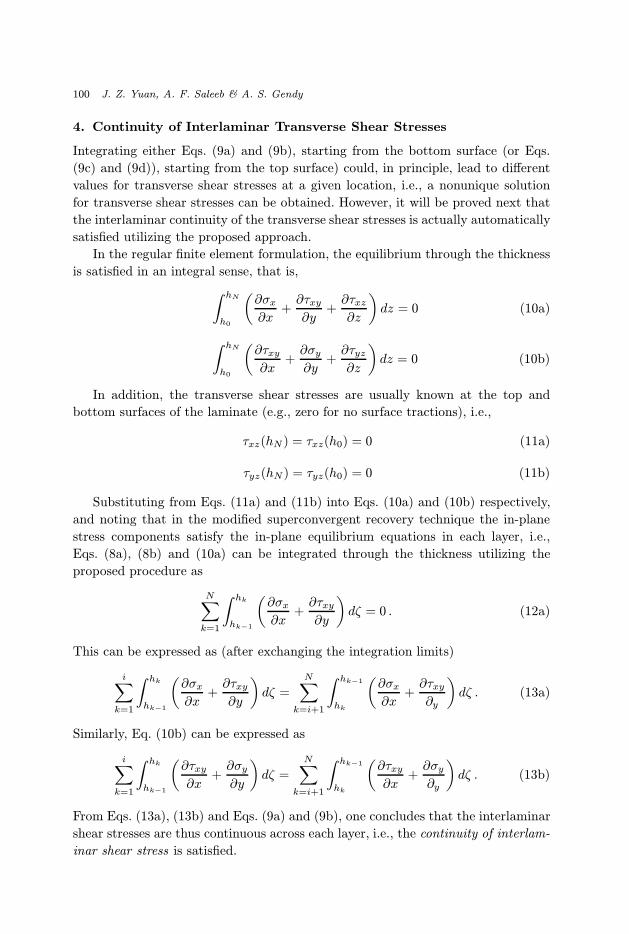
Fig. 23. Variation of the transverse shear stress (τθz) through thickness of a simply supportedlaminated cylindrical shell in cylindrical bending (R/h = 10) (0/90/0).
February 23, 2001 9:43 WSPC/156-IJCES 00003
Transverse Stresses in Laminated Plates and Shells 127
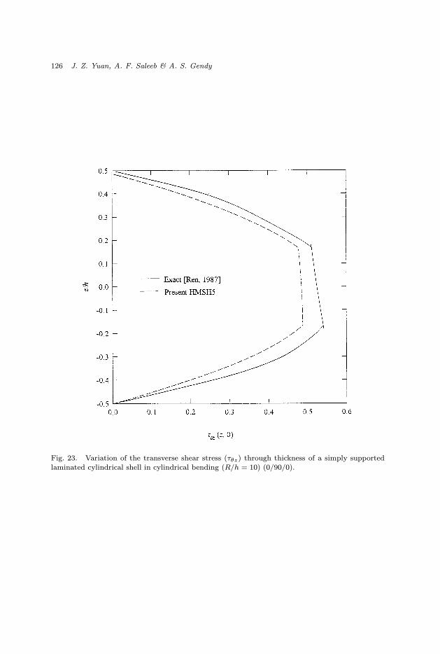
Fig. 24. Variation of the transverse shear stress (τθz) through thickness of a simply supportedlaminated cylindrical shell in cylindrical bending (R/h = 100) (0/90/0).
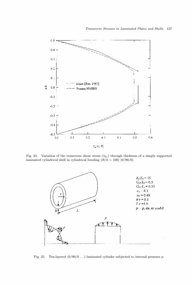
Fig. 25. Ten-layered (0/90/0 . . .) laminated cylinder subjected to internal pressure p.

February 23, 2001 9:43 WSPC/156-IJCES 00003
128 J. Z. Yuan, A. F. Saleeb & A. S. Gendy
Fig. 26. Variation of transverse shear stress (τrθ) through thickness for simply supported ten-layered composite cylinder subjected to internal pressure p = p0 sinπξ cos 8θ.
Remark 6:
Extending the superconvergence patch recovery algorithm from plate to curved
shell structures required more consideration into the curvature effects. Therefore,
the natural coordinates (r, s) have been adopted in each individual patch instead
of global Cartesian coordinates (x, y) in the case of plate. Note that the generated
patch, in general, does not coincide with any of the individual element geometry in
the patch. Therefore, the in-plane stresses at the optimal points provided by the
normal finite element procedure are generally not on the patch surface. As a result,
the accuracy of the superconvergence patch recovery scheme might be somewhat
disturbed. This is demonstrated in the proceeding shell problems in which the
transverse stresses are integrated from the bottom to top surfaces through the
thickness and their values at top surface are all shown to slightly deviate away
from the expected correct values of zero. However, this disturbance can approach
zero with further refined meshes.

February 23, 2001 9:43 WSPC/156-IJCES 00003
Transverse Stresses in Laminated Plates and Shells 129
Remark 7:
From the numerical results provided in Sec. 7.2, one can observe that a good overall
accuracy is generally reached by the proposed scheme, indeed its accuracy is compa-
rable to the other layerwise and higher-order elements for both thin and moderately
thick plates. Furthermore, in terms of computational efficiency, the proposed ap-
proach has shown a greater advantage, since the cost of the post-processing is only
a small fraction of the total analysis cost. That is, the total cost of the proposed ap-
proach is only proportional to the total number of degrees of freedom (5 DOF/node)
of the problem and is independent of the number of the layers considered. For exam-
ple, if the total number of nodes in a problem is N , the total computational cost of
the proposed approach will be proportional to 5N . On the other hand, considering
a “direct” layerwise approach, and in the case of a problem containing a total of N
nodes and a total of M layers, the total computational expense is correspondingly
proportional to N(2M + 3). For the eight-layer laminated problem illustrated in
Sec. 7.2.2, for instance, the total computational cost of the layerwise approach is
almost four times as much as that of the present one.
7.3. Robustness of the projection-layerwise-equivalent approach
A ten-layer cross-ply square plate panel with L = 1, h/L = 0.05 proposed by
Noor and Kim, (1995) has been adopted in this section. The fiber orientation of
the laminates is arranged in the [0/90/0/90/0]s scheme. The panel is subjected to
transverse loading p = sinπx sin πy. The material properties are as follows:
EL = 15 ET = 1
GLT = 0.5 GTT = 0.3378
νLT = 0.3 νTT = 0.48 .
(31)
To assess the effect of mesh distortion on the accuracy of the distribution of the
transverse shear stresses through the thickness, the finite element mesh is distorted
such that the distortion ratio of a1/a varied from 0.5 to 0.2 as shown in Fig. 27. The
transverse shear stresses are evaluated at point A, B and C. The results from the
present approach along with those provided by Noor and Kim, (1995) are presented
in Figs. 28 and 29. As evident from these figures, both approaches perform very
well for this problem. The present approach shows better performance even though
the total number of degrees of freedom used in the present approach is much less
than those in Noor and Kim, (1995) (i.e., 39 versus 54 dof per element).
Different from the model proposed in Noor and Kim, (1995) in which the ac-
curacy of the transverse stresses on the three points (point A, B and C) are com-
parable, the accuracy of such stresses varies in the present approach, as shown in
Fig. 30. It is worthy to note that the patch surrounding point A always contains
the most distorted 4 elements (no matter how the mesh is refined) in the distorted

February 23, 2001 9:43 WSPC/156-IJCES 00003
130 J. Z. Yuan, A. F. Saleeb & A. S. Gendy
configurations. Thus, the transverse stresses at this point are expected to be much
more affected by distortion than the other points (i.e., point B and C). However,
all the results are still comparable with those of Noor and Kim, (1995).
Fig. 27. Simply supported laminated plate for the distortion sensitivity test.
7.4. Hyper-anisotropic cantilever beam under bending loads
This problem was proposed by P. Simacek, V. N. Kaliakin and R. B. Pipes (1993).
It was intended to describe numerical phenomena associated with the analysis of
hyper-anisotropic materials (namely, fiber reinforced thermoplastic composites –
FRTC) possessing a direction of near inextensibility. It poses several challenges in
dealing with element-locking potential (dependent on fiber orientation), spurious
tension modes, etc. Several cases demonstrating some of these numerical difficulties,
for both low-order (four-noded) and higher-order (nine-noded) shell elements, have
been well documented in the above reference.

February 23, 2001 9:43 WSPC/156-IJCES 00003
Transverse Stresses in Laminated Plates and Shells 131
Fig. 28. Distortion effect on the accuracy of the maximum σxz (point A).

February 23, 2001 9:43 WSPC/156-IJCES 00003
132 J. Z. Yuan, A. F. Saleeb & A. S. Gendy
Fig. 29. Distortion effect on the accuracy of the maximum σyz (point A).
February 23, 2001 9:43 WSPC/156-IJCES 00003
Transverse Stresses in Laminated Plates and Shells 133
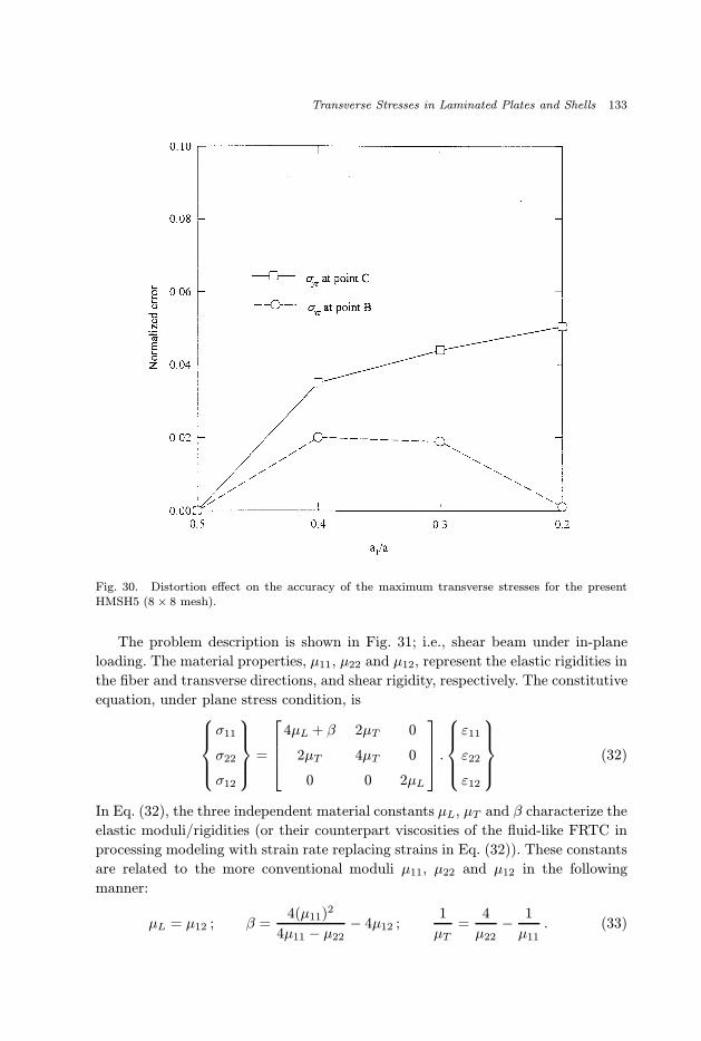
Fig. 30. Distortion effect on the accuracy of the maximum transverse stresses for the presentHMSH5 (8 × 8 mesh).
The problem description is shown in Fig. 31; i.e., shear beam under in-plane
loading. The material properties, µ11, µ22 and µ12, represent the elastic rigidities in
the fiber and transverse directions, and shear rigidity, respectively. The constitutive
equation, under plane stress condition, isσ11
σ22
σ12
=
4µL + β 2µT 0
2µT 4µT 0
0 0 2µL
.ε11
ε22
ε12
(32)
In Eq. (32), the three independent material constants µL, µT and β characterize the
elastic moduli/rigidities (or their counterpart viscosities of the fluid-like FRTC in
processing modeling with strain rate replacing strains in Eq. (32)). These constants
are related to the more conventional moduli µ11, µ22 and µ12 in the following
manner:
µL = µ12 ; β =4(µ11)2
4µ11 − µ22− 4µ12 ;
1
µT=
4
µ22− 1
µ11. (33)

February 23, 2001 9:43 WSPC/156-IJCES 00003
134 J. Z. Yuan, A. F. Saleeb & A. S. Gendy
Fig. 31. A hypar-anisotropic cantilever beam under bending.
It is worthy of note that the ratio between longitudinal, µ11, and transverse, µ22,
moduli in the present case (see Fig. 31) is extremely high, i.e., roughly 108. The
exact solution for this problem gives a constant, in-plane, shear stress of value 1.0,
and a zero normal stress almost everywhere except for two very narrow singularity
regions at upper and lower fibers. This is the well-known phenomenon of “stress-
channeling”. Note that, although the beam is under a bending load, all deformations
are basically of the pure-shear type.
Figure 32 shows the oscillation of “raw” results for the normal stress distribution
through the thickness at the free end. Note also that this oscillation is greatly
reduced after MSPR, but the important feature of two “thin” boundary layers of
stress singularity are still well reproduced.
8. Conclusions
Utilizing a direct two-phase, hierarchical, scheme for laminated plate and shell mod-
els, the in-plane stresses with high accuracy have been recovered on the basis of the
modified superconvergent patch recovery approach. In this, the equilibrium equa-
tions can be satisfied accurately enough to carry out the subsequent calculations
of transverse stresses. In particular, the continuity of the inter-laminar transverse
shear stresses has been shown to be automatically satisfied in the asymptotic limit
of mesh refinements.

February 23, 2001 9:43 WSPC/156-IJCES 00003
Transverse Stresses in Laminated Plates and Shells 135
Fig. 32. Variation of normal stress σx through the thickness at free end.
The proposed approach can be considered as an extension of the equivalent-
single-layer approach. As such, this patch-recovery/stress-equilibrium strategy has
been applied to a mixed shell formulation of the simplest, linear-quadrilateral, type.
The results of the extensive number of test cases and comparisons included here
have clearly demonstrated its effectiveness. Combined together this hierarchical
approach has also led to a formal mathematical proof of the “equivalency” of the
resulting model to the more elaborate descriptions using the layer-wise technique,
at least for the case of flat geometry (and also with sufficient mesh refinement for
shells with curved geometry).
Overall the presented approach possesses a number of advantages. First, being
still built on the underlying simple surface kinematics of the shell element, all such
desirable attributes of low-order models (e.g., reduced distortion sensitivity, inher-
ent simplicity, and their appeal in nonlinear applications) are preserved. Secondly,
with its present simple post-processing format, the approach is quite computation-
ally inexpensive for both linear and nonlinear problems. Finally, the same approach
presented can, of course, be applied to other plate/shell models.

February 23, 2001 9:43 WSPC/156-IJCES 00003
136 J. Z. Yuan, A. F. Saleeb & A. S. Gendy
Acknowledgements
This work was partially supported by the following research grants: National Science
Foundation NSF Grant no. MSS-8816088 and NASA Glenn Research Center, Grant
no. NAG3-1747 to the University of Akron. This financial support is gratefully
acknowledged.
References
1. R. C. Averill, and J. N. Reddy, “An assessment of four-noded plate finite elements
based on a generalized third-order theory”, Int. J. Numer. Methods Engng., 33, 1553-
1572 (1992).
2. I. Babuska, B. A. Szabo, and R. L. Actis, “Hierarchic models for laminated compos-
ites”, Int. J. Numer. Methods. Engng., 33, 503-535 (1992).
3. E. J. Barbero, “A 3-D finite element for laminated composites with 2-D kinematic
constraints”, Comput. Struct., 45, no. 2, 263-271 (1992).
4. Y. Basar, “Finite-rotation theories for composite laminates”, ACTA Mechanica, 98,
159-176 (1993).
5. R. A. Chaudhuri, “An equilibrium method for prediction of transverse shear stresses
in a thick laminated plate”, Comput. Struct., 23, no. 2, 139-146 (1986).
6. S. Di, and E. Ramm, “Hybrid stress formulation for higher-order theory of laminated
shell analysis”, Comp. Method Appl. Mech. and Engng., 109, 359-376 (1993).
7. J. J. Engblom, and O. O. Ochoa, “Through-the-thickness stress predictions for lam-
inated plates of advanced composite materials”, Int. J. Numer. Meth. Engng., 21,
1759-1776 (1985).
8. F. Gruttmann, W. Wagner, L. Meyer, and P. Wriggers, “A nonlinear composite
shell element with continuous interlaminar shear stresses”, Comp. Mech., 13, 175-
188 (1993).
9. T. Kant, and B. S. Manjunatha, “On accurate estimation of transverse stresses in
multilayer laminates”, Comput. Struct., 50, no. 3, 351-365 (1994).
10. T. Kant and B. N. Pandya, “A simple finite element formulation of a higher-order
theory for unsymmetrically laminated composite plates”, Composite Struct., 9, 215-
246 (1988).
11. W. J. Liou and C. T. Sun, “A three-dimensional hybrid stress isoparametric element
for the analysis of laminated composite plates”, Comput. Struct., 25, 241-249 (1987).
12. S. T. Mau, P. Tong, and T. H. H. Pian, “Finite element solutions for laminated thick
plates”, J. Compos. Mater., 6, 304-311 (1972).
13. A. K. Noor and Y. H. Kim, “Effect of mesh distortion on the accuracy of transverse
shear stresses and their sensitivity conefficients in multilayered composites”, Mechan-
ics of Composite Materials and Structures, 2, 49-60 (1995).
14. A. K. Noor and J. M. Peters, “A posteriori estimates for shear correction factors in
multi-layered composite cylinders”, J. Engineering Mechanics, 115, no. 6, 1225-1244
(1989).
15. O. O. Ochoa and J. N. Reddy, “Finite element analysis of composite laminates”,
Kluwer Academic Publishers, Dordrecht, The Netherlands (1992).
16. N. J. Pagano, “Influence of shear coupling in cylindrical bending of anisotropic lami-
nates”, J. Compos. Mater., 4, 330-343 (1970).

February 23, 2001 9:43 WSPC/156-IJCES 00003
Transverse Stresses in Laminated Plates and Shells 137
17. C. W. Pryor Jr. and R. M. Barker, “A finite element analysis including transverse
shear effects for applications to laminated plates”, AIIAJ, 9, 912-917 (1971).
18. J. N. Reddy, “A simple higher-order theory for laminated composite plates”, J. Appl.
Mech., 51, 745-752 (1984).
19. J. N. Reddy, “An evaluation of equivalent-single-layer and layerwise theories of com-
posite laminates”, Composite Struct., 25, 21-35(1993).
20. J. G. Ren, “A new theory of laminated plate”, Compos. Science & Tech., 26, 225-239
(1986).
21. J. G. Ren, “Bending of simply-supported, antisymmetrically laminated rectangular
plate under transverse loading”, Compos. Science & Tech., 28, 231-243 (1987).
22. D. H. Robbins Jr. and J. N. Reddy, “Modeling of thick composites using a layerwise
laminate theory”, Int. J. Numer. Meth. Engng., 36, 655-677 (1993).
23. A. F. Saleeb and T. Y. Chang, “An efficient quadrilateral element for plate bending
analysis”, Int. J. Numer. Meth. Engng., 24, 1123-1155 (1987).
24. A. F. Saleeb, T. Y. Chang and W. Graf, “A quadrilateral shell element using a mixed
formulation”, Comput. Struct., 26, no. 5, 787-803 (1987).
25. A. F. Saleeb, T. Y. Chang, W. Graf, and S. Yingyeunyong, “A hybrid/mixed model
for nonlinear shell analysis and its applications to large-rotation problems”, Int. J.
Numer. Meth. Engng., 29, 407-446 (1990).
26. A. F. Saleeb, T. Y. Chang, and S. Yingyeunyong, “A mixed formulation of C0-linear
triangular plate/shell element – the role of edge shear constraints”, Int. J. Numer.
Meth. Engng., 26, 1101-1128 (1988).
27. P. Seide, and R. A. Chaudhuri, “Triangular finite element for analysis of thick lami-
nated shells”, Int. J. Numer. Meth. Eng., 24, 1563-1579 (1987).
28. M. Di Sciuva, “An improved shear-deformation theory for moderately thick multilay-
ered anisotropic shells and plate”, J. Appl. Mech., 54, 589-596 (1987).
29. P. Simacek, V. N. Kaliakin and R. B. Pipes, “Pathologies associated with the nu-
mercial analysis of hyper-anisotropic materials”, Int. J. Numer. Meth. Engng., 36,
3487-3508, 1993.
30. R. L. Spilker, S. C. Chou, and O. Orringer, “Alternate hybrid-stress elements for
analysis of multilayer composite plates”, J. Composite Materials, 11, 51-70 (1977).
31. R. L. Spilker, D. M. Jakobs, and B. E. Engelmann, “Efficient hybrid stress isopara-
metric elements for moderately thick and thin multilayer plates”, Hybrid and mixed
finite element methods, AMD-Vol. 73, 113-122, (1985) edited by R. L. Spilker and K.
W. Reed.
32. A. Tessler, H. R. Riggs, and S. C. Macy, “Variational method for finite element
stress recovery and error estimation”, Comp. Meth, Appl. Mech. Engng., 111, 369-
382, (1994).
33. J. L. Tocher and B. J. Hartz, “Higher order finite element for plane stress”, J. Engng
Mech. div., Proc. ASCE 93, 149-172 (1967).
34. J. M. Whitney and C. T. Sun, “A higher order theory for extensional motion of
laminated composites”, J. Sound Vib., 30, 85-97 (1973).
35. T. E. Wilt, A. F. Saleeb, and T. Y. Chang, “A mixed element for laminated plates
and shells”, Comput. Struct., 37, no. 4, 597-611 (1990).
36. O. C. Zienkiewicz, and J. Z. Zhu, “The superconvergent patch recovery and a posteri-
ori error estimates. Part 1: the recovery technique”, Int. J. Numer. Methods. Engng.,

February 23, 2001 9:43 WSPC/156-IJCES 00003
138 J. Z. Yuan, A. F. Saleeb & A. S. Gendy
33, 1331-1364 (1992).
37. O. C. Zienkiewicz, and J. Z. Zhu, “The superconvergent patch recovery and a posteri-
ori error estimates. Part 2: error estimates and adaptivity”, Int. J. Numer. Methods.
Engng., 33, 1365-1382 (1992).
38. O. C. Zienkiewicz, and J. Z. Zhu, “Superconvergence and the superconvergent patch
recovery”, Finite elements in analysis and design, 19, 11-23 (1994).
39. R. Zinno, and E. J. Barbero, “A three-dimensional layer-wise constant shear element
for general anisotropic shell-type structures”, Int. J. Numer. Methods. Engng., 37,
2445-2470 (1994).