stress-relieved special grade prestressing strandsdigital.lib.lehigh.edu/fritz/pdf/339_5 .pdf ·...
TRANSCRIPT

RELAXATION LOSSES IN
STRESS-RELIEVED SPECIAL GRADE
PRESTRESSING STRANDS
by
Rabih J. Batal
A Thesis
Presented to the Graduate Faculty
of.Lehigh University
in Candidacy for the Degree of
Master of Science
in Civil Engineering
Lehigh University
May 1970

CERTIFICATE OF APPROVAL
This thesis is accepted and approved in partial
fulfillment of the requirements for the degree of Master
of Science.
Dr. Ti HuangProfessor in Charge
Professor D. A. VanHornC'hairmanDepartment of Civil Engineering
ii

ACKNOWLEDGEMENTS
The relaxation study reported herein is a part of the
research project "Prestress Losses in Pre-tensioned Concrete
Structural MembersTTe The research program is' being conducted at
Fritz Engineering Laboratory, Department of Civil Engineering,
Lehigh University, Bethlehem, Pennsylvania. Professor D. A.
VanHorn, Chairman of the Department, initia~ed the pro~ect in
October 1966. Professor Lynn S. Beedle is the Director of Fritz
. Engineering Laboratory. The sponsors of this research project
are the Pennsylvania Department of Highways and the U. S.
Bureau of Public Roads.
Sincere appreciation is expressed to the three manu
facturers who supplied the test specimens. They are Bethlehem.
Steel Corporation, CF&I Steel Corporation, and United States
Steel Corporation.
The supervision and critical review of this study by
Dr. Ti Huang, professor in charge o·f the thesis and director of
this research project, are sincerely appreciated and gratefully
acknowledged.
The author is indebted to his research colleague, E. G.
Schultchen for his assistance at all times. His previous work
on -the project, as well as his computer program were basic in
~arrying out this study.
iii

Thanks are due "to Mr. K. R. Harpel, laboratory fore
man, and his staff for' their help in preparing the test-setup
and the test specimens.
Thanks are also due to Mr. R. Sopko for taking
valuable pictures, to Mrs. S. Balogh for her assistance in pre
paring the figures in this thesis~ and to Mrs. R. Grimes for
typing the entire manuscript.
iv

TABLE OF CONTENTS
ABSTRACT
1. INTRODUCTION
1.1 Background'
1.2 Purpose" and Objectives
2. RELAXATION IN PREVIOUS RESEARCH
3 • RELAXATION STUDY
3.1 Purpose and Scope
3.2 Test Variables
3.2.1 Manufacturer
3.2.2 Type and Size of Strands
3.2.3 Initial Stress Level
3.2.4 Type of Loading
3.2.5 Other Variables
3.3 Preliminary Investigation
3.4 Additional Tests
3.~.1 Simulation Study
3.4.2 Constant Load Test
4. TEST-SETUP
4.1 Relaxation Frame & Jacking andMeasuring Assembly
4.2 Load Cells
v
1
1
4
6
22
22
22
22
23
23
24
"25
26
26
27
27
29
29
30

4.2.1
4.2.2
Description
Calibration
~
30
30
5. TEST SPECIMENS 3~
5.1 Tension Strands 34
5.2 Distribution and Designation 35
5.3" Force Measurement 35
5.3.1 General 35
5.3.2 Measurement of Initial Tension 3~ .
"5.3.3 Subsequent Measurements 37
5.4 Test Duration and Age 37
6. DATA REDUCTION AND ANALYSIS 39
6.1 . Preliminary Reduction 39
6.2 Method of Analysis 40
6.3 Two-Dimensional Analysis' 41
6.3.1 Computer Program SRELAA 41
6.3.2 Selection of Time Function 42
6.~ Three-Dimensional Regression 47
6.4.1 Computer Program SRELAB 47
6.4.2 Selection of Stress Function 51
6.5 Cqrnparison of the 2-D and '3-D Analyses 53
6.6 Prop?sed Relaxation Equations S4
6.7 Sources of Error 59
vi.

~
7. DISCUSSION OF RESULTS 62
8. CONCLUSIONS 67
9 • TABLES 70 I~n1'1
83
,10. FIGURES ij
j!
1
11. APPENDICES 110
12. 'REFERENCES 139
13. VITA 143
· vii

ABSTRACT
- In this thesis are presented the preliminary ~esults
of a long-term study on relaxation loss of prestressing strands.
This study is part of a research program aimed at the establish-
ment of a reasonable m~thod for the predictibn of prestress
losses in pre-tensioned concrete structural members.
Forty specimens of the 7-wire stress-relieved strands
of the special grade (270 K) were tested, under co-nstant length
conditions, for a duration up to 444 days. The relaxation
specimens represented three manufacture-rs, two strand sizes, and
five initial stresses. Conclusions are drawn as to the effect
of each of these parameters on the 'relaxation loss.
Through a multiple regression analysis, expressions
relating loss to time and initial stress are developed. Two
alternate expressions may be used for the estimation of loss
during t~e initial period up to 500 'days. A prediction equation
is suggested for long-term projection, and is applied for esti-
mating the ultimate loss value at 50 years. The long-term
nature of relaxation is pointed o~t, and predicted ultimate loss
values, for different ·conditions~ are given.
Also included in this thesis is a review of earlier
researches on relaxation of prestressing steel, and summary of
relevant provisions in several foreign and United States design
codes.
\1;I'II
IiII
jI~
$1
1
.
~~~,

1. INTRODUCTION
1.1 Background
The concept of prestressing is quite old, but its 8liC-
cessful application to concrete structures did not start until
the late nineteen thirties. Many engineering and economical
advantages of prestressed concrete over conventional reinforced
concrete were quickly recognized, 'most~important higher resist-
ance to cracking and deterioration, more efficient use of material,. ,
and the greater degree of freedom for the designer. These and
other advantages accelerated the use of prestressed concrete in
many areas of Civil Engineering practice, particularly in the
construction of highway bridges. Linear prestressing in the
United States lagged behind ~hat of many Eur6pean countries. It
did not begin until 1949, when'construction of the famed Phila~3
delphia Walnut Lane Bridge was begun. Since then, the use of
prestressed concrete in bridge construction has become very popu-
lar in this country. As of the mentioned writing, over two
thousand prestressed concrete highway bridges alone, were
authorized by the U. S. Bureau of Public Roads, during the years
1957 to 1960. The State of Pennsylvania~leads all the states in
the nation for the number of prestressed concrete bridges
constructed.
In the analysis and design of prestressed concrete
structu!es, a reasonable estimation of the prestress losses is of

tlle utmost importance. Many factors contribute to the loss of
prestress. For pre-tensioned members, the. losses due to elastic
shortening of the member, shrinkage and' creep of concrete, and
the relaxation of steel are the four major sources.
While elastic shortening occurs immediately upon
releasing of the pre-tensioned strands from their anchorages,
shriwcage and creep are long-term, time-dependent phenomena. The
loss of liquids due to drying or chemical reactions causes short
ening of the member which is known as .shrinkage. Creep refers to
the continued deformation of concrete due 'to sustained external
loading. Relaxation, on the other hand, represents the decrease
of stress in steel under constant strain. This definition, how-
ever, is not strictly applicable to a prestressed concrete member,
where stress as well as strain tend to decrease.
Considering the four major factors, a general expres-
sian may be written for the estimation .of prestress losses, as
recommended by the ACI-ASCE Joint Committee 1 and AASH02
. -In the above equation, ~f represents the loss of prestress, f.s ~
.. .
is the initial stress-in steel. e, e , and e are strains insec
concrete due to shrinkage, elastic shortening,. and creep resp~c-
tively, and o~ is the percentage loss of steel stress due to
relaxation. These recommendations, however, were silent concern-
ing the values of € , € , e and °1 • Instead, a lump sum lossesc
-2-

of 35,000 psi is recommended as an acceptable alternative to
making detailed estimates of each one of these parameters.
In the Commonwealth of Pennsylvania, the design of the
standard pre-tensioned highway bridge member is based on a total
loss of prestress of 20% (35,000 psi) for box beams, and 22.8%
(40,000, psi) for I -beams. For beams not covered by the standard,
the following expression, suggested by the U. S. Bureau of Public
Roads ,30 is used
where
.!ifs = 6000 + 16 f + 0.04 f.cs 1.
f = initial stress in concrete at the level ofcs
centroid of steel
f. = initial stress in steel1.
In the above expression, the 6000 represents the effect
of shrinkage. The term 16 f can be split into two parts,S fcs cs
accounting ~or the effect of elastic shortening, and 11 f es repre-
senting the creep loss. The last term 0.04 f . takes care of the81
relaxation loss. It should be point~d out that the above ·formula
is based on a shrinkage strain of 0.0002, a steel-ta-concrete
modular ration of 5, a creep factor of 2.2, and a relaxation loss
of 4%.
It follows that,at the pres~nt time, the estimation of
prestress losses ,is made either on a lump sum basis , or based on
-3-

a few empirical constants like in the Bureau of Public Roads'
formula. Neither of the two methods reflects the actual nature
of the problem, and both fall short of supplying reliable values
of the prestress loss. So, in an effort to establish a more rea
sonable basis for the prediction of prestress losses in pre
tensioned concrete member, a research project" was initiated in
1966, and is presently being conducted, in Fritz Engineering
Laboratory at Lehigh University, under the joint sponsorship of
the Pennsylvania Department of Highways and the U. S. Bureau of
Public Roads.
1.2. Purpose and Objectives
The objective or "this research project is to arrive at
a rational· basis for the prediction of prestress losses in pre
tensioned highway bridge members used in Pennsylvania., Loss ex
pressions are to be establisheq, and prediction formulae will be
suggeste~. For this purpose the major contributions to prestress
loss are separated from one another to the extent ,possible.
The concrete losses (elastic short~ning, creep, and
shrinkage) are studied in a separate phase of this project. A
preliminary investigation compared the overall characteristics of
concretes from several prestressing plants. In the main study,
two concrete mixes were used and the effects of initial concrete
stress, amount of longitudinal steel, and stress gradient were
investigated. Expressions for the evaluation of" these losses were
devel~ped. Details about these studies and findings are contained
-4-

in Fritz Engineering Laboratory Report 331.1 (May 1968), and
Report 339.3 (July 1969). Further analysis of additional experi
mental data will be performed, in order to modify or confirm
earlier findings.
'The specific objectives of the relaxation investigation,
reported herein, ,are as following:
1. To develop a functional expression for estimating
the relaxation loss of prestress during the first
two years.
2. To establish a prediction formula which estimates
the ultimate relaxation loss over the lifetime of
the member (say fifty years) _,
3. To determine the feasibility 'Of predicting long-'
term prestress loss from short-time data
(100 hours - fourteen days) .
-5-

2. RELAXATION IN PREVIOUS RESEARCH
The plastic fiow of steel under high stress, and con
versely its tendency to lose stress when sub·je.cted to high strain,
has been- reported by the French Professor Vic~t3~ as early as 1834.
This fact was quickly forgotten, however, only to be rediscovered
upon the engineering acceptance of prestressed concrete almost one"
hundred years later. With initial tension as high ,as 175,000 psi,
the "relaxation of steel became a significant factor influencing
the design of a member. Among the first to report about this pro
blem were Redonnet in France22
(1943) ~ and Magnel in Belgium16
(1~44) •
Early in 1946 Ro~ carried out relaxation and creep tests
O? high strength cold-drawn wires 3.2 mm in diameter. He compared
the increase of deformation under constant stress (creep), with
the loss of stress under constant length (relaxation). According
to him, the percentage decrease of stress under constant length
was 50 to 80 percent of the percentage increase of strain under
constant stress." ~7
In 1948, Professor Magnel reported the results of his. .relaxation tests. Cold-drawn wires 5 mm in diamete,r were tested
at an initial stress ~f 123,000 PGi (57% of the tensile strength) .
The loss in stress occurred mainly during the first few hours, and
was ·completed within a period of twelve days. The total loss was
12 percent. He also reported that the loss decreased to 4 percent,
-6-

when a high initial stress of 137,000 psi was introduced and
maintained for two minutes before being lowered to 123,000 psi.
This was one of the very early reports on the over-tensioning
technique for relaxation control.· - 6
In England, Clark and Walley (1953) conducted tests
under a constant length condition. Gravitational loads were
transluitted through a lever system, to develop the necessary
initial stress in the wire. These weights were then removed as
required in order to maintain the constant length. The investi-
gators found that the relaxation ended after 1,000 hours. They
also' observed that relaxation loss increased with increasing
initial stress for levels .higher than 40 percent of the 0.1 per-
cent offset stress.
About the same period of time, G. T. Spare published
26 27a number of papers' in the United States dealing with the
creep and relaxation of high strength wires. His tests demon-
strated that stress-relieved wires showed improved relaxation
char~cteristics and suffered less loss as compared to the cold-
drawn wires, within the practicaL range of initial stresses. For
stress-relieved material at 70% of tensile"ultimate strength some
80 percent of the 1,000 hour loss occurred in the first 100 hours.
After l~OOO hours, the rate of relaxation loss became exceedingly
small, and could be ignored for practical purposes.
Schwier25
in 1955 confirmed Spare's conclusions con-
cerning the superiority of stress-relieved nlaterial' for initial
-7-

stress up to 75% of the ultimate tensile strength. However, a
reversal of this relationship was found at high initial stresses.
Papsdorf and Schwier21
carried out extensive relaxation and creep
tests later, and in 1958 reported their results venturing some
long-term projections. The test results showed clearly that the
relaxation phenomenon did not stop at 1,000 hours. Extrapolation6
from their curves to 10 hours (approximately 114 years) indicated
very high percentages of stress loss, especially for high initial--2
stresses. [e.g. for an initial stress of 165 kg/mm -(230 ksi) ,
85% of tensile ultimate strength of the 4 rom as-drawn wire used
in the test, their curve anticipates a total loss of 21.~~ of
initial stress.]
. 9Everllng confirmed the conclusions already stated about
the relaxation behavior of stress-relieved wires and strands as
related to the applied initial stress. He also found the' relaxa- .
tion loss to be dependent on the speed of loading 0 Slower loading
leads to smaller relaxation loss.
Report No. 14 of C.U.R. (The Dutch Committee of
Research), Delft (1958) contained the results of relaxation tests,
which also showed that stress-relieved strands demonstrate higher
losses at very high ranges of initial stress.
A new technique was used by McLean and Siess1.5, for mea
suring the force in their relaxation specimens. The tensioned
wire was electromagnetically excited into force~ vibration. The
frequency.of the input was altered until reso~ance took place.
-8-

With help of available calibration curves, the stress correspond-
ing to the resonant frequency which is the actual stress in the
wire, was calculated. This method yields high accuracy in
measurement.
Dr. rng. S. Kajfaszl~ of Poland performed a number of
relaxation tests on single and twin-twisted prestressing wires
(1958). Based on a statistical analysis, Kajfasz obtained a
number of experimental equations from which he derived the general
expression:
IJ.fr
= C (log t - log t )e e 0
b.f ::: relaxation in stress units (kg/mm 2')
r
t· = time in minutes at which first reading was madeo
t . ::: time in minutes
c = a parameter depending upon the ratio of initial
stress,f.,to 0.2 percent offset stress,f .. . 1 Y
{
Kajfasz suggested a linear relationship for C:
f.C = 2.41 (f.
1) - .1.395
y~
Including the relaxation loss prior to the first read~
ing,6£ ,Kajfaszts equation takes the following form:ro
-9-

f.!:J.f =[2.41 Cf
1) - 1.395J
r y(log t - log t ) + 6fe eo' ro
It is interesting to note that for an initial stress
level of 0.58 f , C = 0 and ~f = ~f, indicating negligibley r ro
relaxation loss.
Stussi28 in 1959 developed a TTlaw of long-term relaxa-
tionTT using experimental results obtained from relaxation tests
performed on cold-drawn wires, 7 mm in diameter and with initial
stresses varying from 60 to 75% of the ultimate strength. His
study showed clearly, that the higher the initial stress, the
higher will be the prestress loss. With remaining stress after
relaxation plotted against'" logari thm of time, it was found that
all curves contained a point of inflection beyond which" time, the'
decreasing stress asymptotically approached a common lower limit.
StuBsi defined this lower limit as TTrelaxation limit TT (0 ). Fora
the kind of wires he was ,using, this limit cam~ out to be 0.53 of
the ultimate strength, lying somewhere near the proportional
elastic limit at 0.01 percent offset. From a practical" point ofview, it would not be reasonable to prestr~ss the tensioning steel
far beyond this limiting value.
A comment on the foregoing study of Professor StuBsi was. " 2S
released by The Dutch Committee (Betonstaal) in 1960 . The
validity of Stussi T s "Relaxation Law" and the material constant cra
was seriously questioned. The Committ"ee noted that' the formula
-10-

derived by St·ussi did not agree with a number of e'arlier relaxa-
tion curves. It questioned 'further the method of extrapolation
used by Stussi, and contended that the value cr , even if it were. . a
to exist, would have little practical significance.
Around this time the ACI-ASCE Joint'Committee 1 323 gave
a general expression for evaluation of prestress losses. In their
expression
~f = (e + e + e ) E + 51:f.S esc s ,,1
the part 0lfi represented the loss due to relaxation of steel.
Although sound in principle, the ACI-ASCE expression did not P~o-. _,
vide any suggestions in the, estimation of the concrete strains,
nor the relaxation percentage 8i -
An interesting investigation by Kingham, Fisher and
Viest12
was carried out as part of the AASHO ROAD TEST bridge
research program. Indoor relaxation tests of 20 specimens were
reported. Prestressing cables made up of parallel O.192-in. wires,
.and 7-.\vire strands 3/8-in. in diameter were used. .T_he duration of
their tests varied from 1,000 to 9,000 hours. Three basic re-
quirements underlined the mathematical model used.
-11-

The formula suggested was:
bfr
d(1 - e
-t/. ba)
. Observing the approximately, linear relationship between-th t
log b.f and logt, the factor (1 - e a) was replaced by / a. Thusr
the formula was transformed into:
. f .. d b. ~fr = g f
i(fl) t
U
in which
6f = relaxation stress loss at time tr
f. = initial stress1..
f = ultimate strength of steelu
t = time from application of initial stress, in hours
g, d, b = constants determined by regression analysis. For
the strand the values of g, b, and d were 0.0488, 0.274 and 5.04
respective.ly. The authors recommended that their equation be
used up to 9,000 hours, representing the upper limit of their test
data. No information on ultimate loss was provided.
In 1963 a study was made" by Callill and Branch 4 on relaxa-
t"ion ,of a new wire product, the "stabilized wires". A new method
of extrapolation was used based on established linear relationship
between log strain and log time. For this kind of extrapolation,
one would have to determine the load loss rate at 1 hour and the
.-12-

slope of the log load loss VB. log time plot. These are necessary
to determine the constants in the prediction equation. CahillTs·
extrapolation over 30 years, showed that .the new material
suffered less loss than a stress-relieved strand.
An extensive investigation on this subject was carried
out at the University of Illinois during the early 1960's.
Magura, Sozen, and Siess19
reported their results in 1964, to-
gether with an extensive review of work done by previous re~
searchers. The 'object of their investigation was to study the
effects of time, level of initial stress, type of wire, and pre-
stretching on the relaxation loss of prestressing wire. The
authors arrived at an equa~ion which relates the remaining stress
to time and initial stress. The expression is:-
f sr=1
"1 _ log t10 0:.55 )
where
f. "for fl ~ 0.55
Y
f s = the remaining stress at a~y ·time after prestressing
f. = initial "stress at r~lease1
t = time, in hours
.fy = yield strength
In the usage of the above formulation, the loss occurring
-13-

before release should be subtracted from the total loss predicted,
with f. taken as the effective stress at release.1.
The authors stated that it is 'not strictly justifiable
to project the conclusions from their test to longer durations
and different conditions. K. Prestonl
of C F &.r Steel Corporation
suggested rearranging the previous equation to evaluate directly
the loss of stress
~fr
where
= log t10
f.1( r - 0.55)Y
f.1
~f = stress loss due to relaxation t hours afterr . ;'.
initial str~tching.
Preston ~lso pointed out that to account for the strain variation
due to elastic shortenin,g, creep, and shrinkage of concrete, the
foregoing formula should be applied to small increments of time.
It is suggested that at least three time increments be used:
namely, initial stretching to transfer, from transfer until
application of permanent load, and ~inally t~ll the end of the
service life of the member.
In a paper p~esented before the Australian Institution
of Engineers in 1965, J. M. Antil13
reviewed earlier researches ont
relaxation and included a number of conclusions and suggestions.
Contrary to earlier conceptions, the relaxation loss at 1,000
hours represents less than half of the" ultimate loss. The rate
-14-

oof relaxation increases rapidly with temperatures above 20 C.
For initial stresses below 0.50 ultimate strength, the relaxation
loss may be considered neglibible for practical purposes. He also
asserted that a high degree of accuracy in the estimation of loss
values i~ not warranted, since the quantity of practical signifi-
cance is the residual stress remaining in the tendon.
A five-year investigation was carried out at the Univer
sity of New South Wales in Australia. A. J. Carmichae15
reported
in 1965 the results of this study. The test results showed that
the stress relaxation continued far beyond 1,000 hours. The ratio
of stress loss at 10,000 hours to t~at at 1,000 hours was 1.34 for
O~161-in. diameter wires, ~nd 1.40 for O.20D-in. diameter wires.
Further work has indicated the average stress loss at 59,POO
hours to be 1.6 times the stress loss at 1,000 hours. An
eguation.bas~d on basic creep laws was developed and suggested as
a promising prediction equation. Also, the equation suggested by. .
Magura, Sozen, and Siess seemed to be satisfactory up to 1,000
hours.. 8
Engberg of Sweden reported in 1966 that his test
results showed the stress relaxation to bea linear function of
the logarithm of the testing time. The total relaxation after
foqr years was 9.5 percent for the preloaded wire, and 10.25
percent. for the wire tested as delivered. By linear extrapolation,
it was found that the two curves corresponding to t4ese test speci-
mens, intersect after some sixty years at a stress ~elaxation of
-15-

about 13.5 percent .
. ·In a first draft of TtRecommendations for Estimating
Prestress Losses Tt (1969), the pcr Committee on prestress losses
suggested that for stress-relieved prestressing strands, the
following equation' shall b~ used for the estimation of relaxation
loss.
f = [1slog t
10
f.( f
1- O. 55) ] f i
y
f.1-
for r ~ 0.60Y
This is the same formula suggested by Magura, Sozen, and Siess,f.
1except that the limiting value of r has been increased slightly.y
For other types of prestressing reinforcement, the Committee
suggested using manufacturerTs recommendations with the support
of adequate test data.
Recommendations on steel relaxation given in various7 .
foreign codes may be categorized three ways:
1) Qualitative discussion (Germ~~y, Austria, Finland,
Poland) .
2) Flat rate, or flat value (Denmark, Italy, Belgium,
England) ..
3) Detailed procedure, or suggested equations (Russia,
Holland, European Concrete Committee) ..
-16-

TIle German and Austrian Codes (1953 and 1960 respec-
tively) refer to creep in steel, and indicate that it will become
noticeable only if the stress is above the creep limit. They
also note that creep ceases within a few days if the stress is
sufficiently below the ult~mate tensile strength. Over-stressing
the steel can cancel the effect of creep.
The Finnish Code (1958) deals very briefly with relaxa-,
tion of steel, and requires relaxation tests to be performed for
a durati9n of at least 120 hours.
According to the Polish Provisions, the relaxation
losses may be neglected for steel wires of diameters 1.5 and
2.5 mm, if maximum stresses are maintained within the permissible
limits. Similarly, it is permissible to neglect relaxation
losses in wi~es of diameters·5 and 7 mm in post-tensioned elements
if, befo~e anchoring, the steel is over-stressed. Over-stressing
is to be achieved by increasing the given maximum stress in steel
. by 10% and maintaining it at this level for at least ten minutes
before anchoring.
The Danish Code, as early 'as 1951, 'contained quantita-
tive provisions on the creep strain of steel. The following
values are specified:
for f. 0.80 f N 0.1' 0.2%= €PL ,...., -1 U
for f. 0.75 f I""'J 0.05%= e ("OJ
1 U PL
for f. = 0.45 f epL
~ 01 U
-17-

The following guidelines are contained in the Italian
Code (1960):
1. "In the case of beams post-tensioned with cables,
relaxation losses can be taken as 7% of the initial tensioning
stress. tT
2. "In pre-tensioned beams these losses can be taken
as 12~ of the initial stress if the tendons are individual wires,
and as 14% if the tendons are strands. tT
3. "The loss of stress over an infinite time can always
be estimated as twice the average on at least two specimens sub-
\jected to 120-hour relaxation tests at the initial tensioning
stress in the case of post-tensioned beams, and at 2. 5 times 'that
average loss in the case of pre-tensioned beams. TT
The Belgian Code (1960) contai~s an overall estimate of
the total loss including elastic shortening, shrinkage, creep, and
relaxation of steel. For pre-tensioned tendons directly embeded
in concrete the recommended value is 20% of the initial prestress,
provided that the stress in the tendons at'time of transfer exqeeds2
60 kg/mm (84ksi).
The British Standards Institution (1965) tentatively
recommended a flat vlaue for the loss of stress due to creep
of steel. A value of 15,000 Ibf/in.2
for stress-relieved wire,
or where the wire is over-stressed by 10 percent of the initial
-18-

str~ss for a period of two minutes during tensioning. Any further
reduction should be based on tests of at leas~ 1,000 hours dura-
tion with an initial stress of the tensile strength of the wire.
-The Russian Code recommends the following formula for
14computation of the ultimate loss due to relaxation of steel. '
In high-strength cold-drawn wire
Lifr
f.1
= (~.27 fu
0.1) f.1
In hot-rolled reinforcement
f.af
r= 0.4 (0.27 fl
u
If f. ~ 0.37 f , 6f = 01 - U r
where
,Af = loss in stress unitsr
f. = initial stress value1
o.1) f.1
f = ultimate strength of steelu
It is interesting to note that the Russian Co~e 'anticipates re
laxation losses for initial stresses as ~ow as 0.37 f. Manyu
studies set this value not less than 0.50 t .u
The Dutch Code (1961) explains the dependence of the
relaxation upon the ratio of the initial stress to the guaranteed
tensile ~trength of the steel and upon shrinkage and creep strains
in the concrete. A table'is provided which gives the loss as per-
-centag~ of initial stress. For usage of the table, 'the values of
-19-

the initial stress, shrinkage and creep strain are required.
Linear interpolation b,etween the values of the table is permis-
sible-.
In their recommended practice for prestressed concrete,
(June 1966), the eEB (Comite' Europeen du B~ton) suggested the
following procedures for estimating relaxation loss:
1. "The relaxation diagram, of the steel, tested at
constant length and temperature, as a function of time and of the
value of the initial stress applied to the steel should be deter-
mined experimentally. For practical use the relaxation diagram
should account for actual conditions including temperature. TT
2. 1TThese diagrams should be plotted for ini~ial
stresses respectively equal to 65% and 80% of the characteristic
failure strength (f) of the steel. For an initial stress inter-. u
mediate between these two values it is permissible to apply linear
interpolation. Tf
3. "The particular relaxation value at the end of 1,000
hours is to be considered. In experiments ..~arried out, the
follo~ing values were observed at the end of 1,000 hours: for an
initial stress equal to 0.65 f the relaxation values were beu
tween 2% and 8% of that initial stress; for an initial stress
e.qual to 0.80 f the relaxation values were between 8% and 1~;6u
o'f that initial stress. Tf
-20-

4. "The tangent at the point of the diagram correspond
ing to 1,000 hours, will allow extrapolation up to a period of
100,000 hours. It should be endeavored as far as possible to
check the slope of the tangent bY,comparison to a long-term test
performed on a specimen of similar steel. TT
'In summary, at the present time, research work is being
done on the relaxation of steel, but has not yielded sufficient
long-term information. Qualitatively, the phenomenon was de
scribed and its nature clarified. The factors that affect relaxa
tionloss were identified and the long·~term nature of relaxation
expe~imentally proved. Quantitatively, several investigators
attemp~ed to formulate expressions for prediction of the stress
loss. The proposed expressions generally fit th~ test data used,
but their validity for prediction, particularly for long-term
projection, remained unproven.
-21-

3. RELAXATION STUDY
3 .1· Purpose and, Scope
Relaxation of prestressing strands is significant be
'cause of the high level of stresses. Many of the ear~ier
researchers of relaxation stress loss claimed that the stress
would reacll a stable state in' a few hours and that the relaxa
tion loss represented onJ.y a very small fraction of the initial
stress. More recently, however, test ·results of longer duration
have become available, and it has been estab'lished that relaxation
·does extenq over a long period of time, and that it could amount
to as high as 20% of the initial stress.
It is the ultimate purpose of this project to provide
an expression for the prediction of _relaxation loss, accurately
over a short period (one to two years), and reasonably well for
the total loss over the entire "life of the structural member (say
at the end of fifty years) .
It is also speculated that the relaxation loss for the
life of the member may be predictable from short-time test data
(100 hours - 14 days). This possibility will also be investigated.
3.2 Test Variables
3.2.1 Manufacturer
The three main suppliers of prestressing strands in
Pennsylvania are: Bethlehem Steel Corporation, 'CF & I Steel
--22-

Corporation and United States Steel Corporation. The prestress
ing strands from all three manufacturers are subjected to ASTM
standards. However, due to differences in the chemical composi
tion, the kind and extent of treatment, and other factors, a
difference in their relaxation behavior could be expected.
Therefore, prestre,ssing strands from all three manufacturers were
included in this study.
3 . 2 _2 Type and Siz.e of St.rands
Since the study is mainly concerned with prestressed
bridge members-, wherein 7-wire stress-relieved strands of the
special grade (270 k) are used almost exclusively, only this type
of strand was tested. Two..strand sizes, 7/16 in. and 1/2 in.
nominal diameter, were included.
3.2.3 Initial Stress Level
. In all of the previous investigatiollS dealing with the
relaxation problem, the importance of the initial stress level
and its direct effect on prestress loss were recognized. In this
investigation, three primary stress levels were selected, repre
senting an upper limit, a lower limit, and an intermediate value
Qf the initial stress. The three values are, respectively: 80,
50, and 65 percent of the guaranteed ultimate tensile strength
.(GUT~). The 80 percent value, which is ~lightly below the con
ventional yield strength of the strand, can be looked upon as the
practical upper limit of the initial stress. The 50 percent, on
-23-

the other hand, is selected as a lower limit, below which the re-
laxation loss can be neglected. The intermediate stress level of
65 percent is chosen at approximately the same value as prevailing.
in an actual pre-tensioned bridge member immediately upon transfer.
It is noted here, that the European Concrete Committee (CEB) rec-
ommended the establishment of relaxation curves at similar initial
stress levels, 65% and 80% of the characteristic failure strength
respectively. An additional stress level of 70% was used in two
of the test specimens. The purpose is.to qetect any abrupt
change in the relationship between the behavior of the strands
and the initial stress level near the conventional yield
strength level. Two 7/16-in. strands from manufacturer B,
fractured before reaching the intended 80% initial stress level.
Their replacement specimens were tested at a slightly lower
initial stress level of 75% GUTS.
3.2.4 Type of Loading
Theoretically, creep is defin~d as the increase of
strain under constant load or constant stress. Relaxation is the
decrease of stress under constant strain. Both phenomena share~ .... ,
the property of being time-dependent and are principal factors in
any long-term. study involving stresses and strains. The data
obtained ·from a constant load test are strain quantities (creep
strain), while the results of relaxation tests are given in the
form of stress quantities (prestress loss).
The actual experience of a prestressing strand
-24-

contained in a concrete member is different from both of the
above. Because of the creep and shrinkage of concrete and fluc-
tuations in superimposed loads, the length of the concrete
member, and consequently the leng.th of the strand changes.. This
change of strain causes a deviation from a pure relaxation type
of situation. At the same time, the tendon is relieved from
some of its·stress, and the basic condition for creep is violated.
In the actual situation, a decreasing strain is combined with a
decreas~ng stress. Nevertheless, th~ conditions are more com-
parable to that of a relaxation test than that of a creep test.
For this reason the major part of the tests in this investigation
were constant length (rel~xation) tests. Description of relaxa
tion specimens will be given in Chapter 5.
3.2.5 Other Variables
. There are a number of other variables that might affect
the relaxation loss. Temperature variations can have a signifi~
cant effect on relaxation. An investigation by Mikhailov and
· h 1 20 h h·· 1Kr~c evs<aya sowed t at lncreaslng temperature resu ted in a. 26
considerable increase in stress loss. Schwier found that ano 0
increase of temperature from 72 F,to 212 F magnified relaxation
losses eight times.
It has also been reported that maintaining a high
stress for a shor~ period of time before anchoring to the desired
initial stress (prestressing or prestr~tching) results in an
appreciable reduction of the relaxation losses.
-25-

These effects of temperature variations, prestressing,
and other factors were not ,included in this study.
3.3 Prel{minary Investigation
. "Preliminary results on "34 constant length (fixed strai~
• ~4specimens indicated the following concluslons: -
1) The relaxation loss ~epends strongly on the initial
stress in the strand.
2) In general, 1/2 in. strands suffer a higher relaxa-
tioD loss than the 7/16 in. strands.
3) The loss characteristics from the three manufactur-
ers do not differ signifiq~ntly during the initial pe~iod.
Details of these preliminary observations are: contained·
in a report by E. G. Schultchen, at the Lehigh Prestressed
Concrete" Committee meeting, July 1969, and in Progress Report
No. 3 of the project (Fritz Engineering Labora~ory Report
No. 339.4, by Schultchen and Huang) .
3.4 Additional Tests
The relaxation stress-time curves can be visualized as
contour lines on a surface in the stress-strain-time three-
dimensional space, as shown in Fig. 1. " A surface can be es~ab-
'lished from the relaxation· test data, and information regarding
constant load or other specified strain variations can then be
derived from this surface. To verify the results of such
-26-

operations, additional tests are included in this study, but
their results are not included in this report.
3.4.1 Simulation Stud~
As was pointed out earlier, the actual situation of a
prestressing strand under load is neither purely relaxation, no~
purely creep. In an effort to simulate actual conditions, twelv~
simulation specimens were fabricated and are being tested at
Fritz Engineering Laboratory. Each relaxation specimen is a pre
tensioned concrete, member with a concentric unbanded prestressing
strand. It is believed that the concrete would provide a strain
variation'similar to that of the actual member. Tensile force
remaining in the strand is..measured in a manner similar to the
relaxation specimens according to a preset schedule. Simultane
ously, concrete strain readings are obtained by means of a
Whitemore gage, from a number of gage points on the four face$ of
the specimens. The data obtained has not yet been analyzed and·
no conclusions can be made at this stage.
3.4.2 Constant Load Test
"Creep and stress relaxation are kissing cousins but
they are not interchangeable", CT. C. Hansen1d). In the quoted
paper, Hansen suggested an approximate method for estimating' one
.from the other that gives good results for stresses well below
creep rupture. In 'his equation, creep strain and stress after
relaxation are related, with the values of the initial stress and
-27-

initial strain as parameters.
Reference is-again made to the three-dimension sur
face relating stress, strain, and time, from which iriformation
regarding creep can be derived. To verify the results of these
computations six constant load (creep) tests will be performed.
-28-

r 4. TEST-SETUP
~.l Relaxation Frame & Jacking and Measuring Assembly
The relaxation frame is made up mainly of two
6 in. x 4 in. x 1/2 in. steel angles, with long legs upright and
1 in. apart. Thia loading frame is 10 feet in length and is
supported near its ends on a steel storage rack designed espe
cially for this purpose. Five plates at 2 ft.-3 in. spacing are
tack welded to 'the outstanding legs of the double-angle section.
To maintain the back to back distance between the long legs,
seven spacers are used at spacings of 1 ft.-6 in. The strand
specimen is placed at the centroid of the double-angle section
and anchored to 1 in. end plates by means of strand chucl<s.
Fig. 2 shows some details of the loading frame, while Fig. 3
~ives, a general view of the complete setup.
The jacking and measuring assembly consists of a
number of parts extending between the end plate at the jacking
end of the frame and the pulling rod of the hydraulic jack. As
Schematically shown in Fig. 4, the end plate 'and the strand chuck
are separated by a load cell and a device for the control of the
initial elongation in the specimen. The device is composed of a
number of spacers, D, and a fine adjustment bolt, B, which screws
into the bearing plate A. Fig. 5 shows the jacking end of the
frame with the above-mentioned arrangement.
For the detection of possible strand slippage in the
~-29-

Strandvfses, dial gages were mounted on top of each end plate.
The plungers of these dial gages rested against targets attached
to steel straps clamped on the strand specimen. Readings on the
dial gages were taken on both ends of the frame -before and after
each force measurement, for ~ period of fourteen days starting
from the initial stretching.
4.2 Load Cells
4.2.1 Description
The load cells used for the force measurement were
especially made for this investigation. These are hollow cylin
ders made of 20l4-T6 aluminum alloy. They are 5 in. long, and
have_an inner diameter of 7/8 in. and an outer diameter of
1-3/~ in. Eight EA-13-125TM-120 type strain gages are mounted
on the outside of each cylinder, four in the longitudinal direc
tion, and the other four lateral. These strain gages are con
nected into two independent Wheatstone Bridges~ Strain readings
are taken from the bridges by a digital strain indicator (Bean
Model 206B) .
4.2.2-, Calibration
The test data used in the analysis are readings obtained
through the load cells. In order.to guarantee maximum reliabil
ity, much attention was paid to the handling of the load cells,
~nd a careful procedure was followed in their calibration;
Two series of load cells (Series A and 0) ,'were used in
--30- . '

the relaxation study. Load cells were calibrated .five or six :tn
series on a Tinus Olsen 120K-hydraulic testing machine at Fritz
Engineering Laboratory. Two loading and one unloading runs were
performed. The calibrated range of loading was from 1 kip to
34 kips. Readings were taken at each multiple of 5 kip, as. well
as at the limits of the loading range.
A computer program (PROGRAM CALIB) was written to per
form regression analysis for the calibration data. It should be
pointed Qut that the actual loading, as opposed to ,the nonlinal
loading, was recorded and used in the regression analysis. The
final calibration coefficients were determined by the following
procedLlre:
1) A regression analysis is performed based on all
raw data.
2) Based on results of step (1) data points with
large deviation are rejected, and a new regres~ion analysis is
performed based on all data remaining. (Criterion for rejection
was chosen to be two times the standard error of estimate, SEE.)
3) The above procedure, steps 1 ..and 2, W~S used
twice.for each bridge ~hannel:
(a) Expressing Indicator readings -in terms of
Load readings I = A.L
(b) Expressing Load readings in terms of
Indicator readings'L = B.I
-31-

The aver'age of B and the reciprocal of A is used for later force
determination.
The ,calibration data for Series A showed some abnor
mality, as shown in Fig. 6. The following modification was used
in their regression analysis:
1) Data obtained from the unloading run was excluded
from the regression analysis because of obvious bias (hysteresis
type of off-set) .
2) Data from lowest load step (1 kip) were also
excluded because of the large error included in the load readings
of the lower range of the testing machine.
Fig. 6 is a qualitative picture of the path followed at each run
and the data excluded.
It should be pointed out~ that even after modification,
a few load cells of Series A (data sets 8 and 9) still showed a
certain amount of bilinearity. However, since. no prefgrence
between runs 1 and 3 could be made, both runs were used in the
analysis.
As a result of the regression analysis the following
conclusions were drawn:
1) In" the majority of 9ases, the load correction
improved the prediction relationship. In series 0 which included
25 load cells, or SO channels, the standard error of estimate was
~~educed for 26 channels. In series A, 48 out of 62 channels
-32-

showed improvement 'upon inclusion of load correction.
2) The difference between calibration coefficients B
and kis not significant, except for those data with bipolarity
(Series A,.data sets 8 and 9).
The results obtained from the above-mentioned analysis
show that' each unit of the indicator reading corresponds to a
force of approximately 8 pounds, which is less than 0.06 perc~nt
of the initial tension in the specimen. The range- of this cali
bration constant was from a lowest value of 7.89 pounds per unit
reading to a highest of 8.13.
-33-

5. TEST SPECIMENS
5.1 Tension Strands·
In the United States, prestressing tendons for pre-
tensioned bridge beams are almost exclusively uncoated seven-
wire stress-relieved strands. The standard strands (ASTM A-416)
are maqe of high-carbon steel. The raw material, in the form of------
rods, was heat-treated and then cold-drawn into wires of small
diarrleter. Strands are made of six wires twisted around one
central straight wire of a slightly larger diameter.
Stress-relieving is a controlled time-temperature
heat-treatment process. By heating the strand to a controlled
temperature, residual stresses induced during manufacturing and
stranding are relieved without destroying the fibrous structure
of the material. This process also increases the elastic limit
and the ductility of the strand.
A-416 standard strands are required to hav~ an ulti-
mate tensile strength of 250 ksi. In 1962, a special grade of
strands, with an ultimate tensile strength of 270 ksi was intro-
duced, and quickly dominated the pre-tensioned prestressed con-
crete "industry. Coupled with a slightly larger ·size, tIle strands
of 270 k grade have a load capacity approximately 15% higher than
the standard strands of the same nominal diameter.
The specimens included in this study were stress-
relieved 7-wire strands of the special grade. Tensile tests were
.:.34-

'performed on the strands after their shipment to Lehigh University.
Results of these tests and other information relevent to the
tested strands are compiled in Appendix 1.
5.2 Distribution and. Designation
A total of 40 relaxation specimens were tested, repre
senting three manufacturers, two strand sizes, and five initial
stress levels. Table 2 shows the distribution. of specimens for
each combination.
Each specimen was designated by a two-letter, two
number, individual cod~.' The first letter refers to the strand
size. The second ident'ifies. th.e manufacturer. The· first numeral···.
designates the initial stre"ss level, while the second identifies
the several repetitive speci~ens in sequential order. Fig. 7
provides a key to this designa~ion with all possible combinations.
5.3 Force Measurement
5.3.1 General
'Th~ main requirement in force measuring for relaxation
tests is that the measurement must be accomplished while the
strain is maintained constant. Various methods had been used in
the past. They generally fall into one of four major categories:
the vibration method, the lever method, the balance method, and
the deflection method. A short description of each can be found
on page 14 of Reference 19.
The method used in this study involves direct
-35-

measurement of the force by means of a carefully calibrated load
cell, connected in series with the test specimen. This technique
is similar to that employed by the balance method.
The axial deformation of the load cell is small com
pared to the length of the tested strand and can be neglected.
This· will be further discussed in Section 6.5.
5.3.2 Measurement of Initial Tension
At the initial stretching of a relaxation specimen, an
additional load cell (G) is used outside of the 'jacking ram in
conjunction with the internal load cell (E), as shown in Fig. 4.
At the Qeginning, a zero reading on the internal load cell is
taken, and the desired final reading after anchoring is calcu
lated according to the desired initial stress.
The strand is stretched until the. external load cell
shows a ·load slightly higher than the required value. Several
spacers are placed between the adjustment screw (B) and the
load cell (E), as shown in Fig. 4. The adjustment screw is then
turned out of the end plate until a snug fit is reached. A few
repetitions are sometimes needed until the desired internal load
cell reading after anchoring is accomplished. Tables 2 and 3
give the actual initial stress percentages obtained for each
specimen. As can be seen, the values are quite accurate. The
maximum deviation from the desired value was only 0.7%. In the
majority of cases, this deviation was .less than 0.1%.
-36-

5.3.3 Subsequent Measurements
For subsequent measurements, only the internal load
cell is used. The procedure of measurement includes the follow
ing three steps:
1) Taking readings on the loaded internal load cell.
2) Pulling on the strand coupler until pressure
between the spacers disappeared. This can be detected by hand
touch of these spacers. The load cell is now under zero load.
The current zero readings are taken.
3) Without changing the settings of the spacers or
the adjustment screw, the jack is released. A second set of
readings is taken on the reloaded internal load cell.
The reason for excluding the external load cell in sub
sequent force measurements, is" that the internal load cell yields
much more reliable and consistent results. This is discussed
further in Section 6.5.
5.4 Test Duration and~
Readings after initial stretching are taken according
to a preset schedule. In Table 4 are given the selected inter
vals up to 2,000 days. In the early stage, readings are taken
in very short intervals, which become longer as the specimen ages.
It was pointed out earlier that relaxation of steel is
a long-term phenomenon, which may not be completed within the-
-37-

duration of a test program, which usually does not e.xtend over
more than five years. Consequently, the significance of any
study depends on the length of its test program. As of
February 1, 1970, the age of the oldest specimens i.n this inves-
tigation is 444 days (approximately 10,000 hours), twelve speci-
mens have reached this age. Forty percent of all specimens have
been under tension more than 300 days; sixty-five percent more, "
than 200 days, and ninety-five percent more than 100 days.
In spite of the relatively short age of these specimens,
·it is felt that a reasonable estimate of the prestress loss could
be made based on the information collected.
-38-

6 • DATA REDUCTION AND ANALYSIS
6.1 Preliminary Reduction
The experimental data collected in this investigation
is indicator readings from the calibrated load cells. Each load
cell yields two sets of data at each force measurement, one from
each channel. Each set of d~ta consists of three readings, two
loaded readings before stretching and after,release of the speci-
men, and one zero reading when the force in the specimen is com-
·pletely resisted py the _jac'king assemblage. Thus, two differen-
tial readings are obtained for each channel. The average value
of the two is taken, and is used in further analysis. Conse-
quently, for each force me·asurement two pieces of data (averaged
differential, readings) are obtained" and each is directly pro-
'port.ional to the force remaining in the strand, by means of the .
respective calibration constant. These hand-reduced differential
readings are used as input data for a computer program (LISTREX) ,
which performs the preliminary reduction. This program reduces
the input data into the percentage loss· of force in specimen.
Basically the following operation is performed in this early
reduction:
Percentage Loss = Initial Force - Remaining ForceInitial Force
'At this' stage, the loss values are carefully examined for unusal
-39-

va.ri?-tions" and the i-nput data, which are ,reproduced in the com-
puter output, are inspected for possible errors in hand calcula-
tions, card punching, and otherwise.
6.2 Method of Analysis
The problem of developing expressions for relaxation
'loss of steel, based on experimental data is, by nature, a sta-
tistical type of problem. It involves an' attempt to find the
geometric best fit of the available data. There is an additional
complication. The selected expression must be suitable for the
purpose of prediction over a long period of time, for which test
data are not available.
The first step of the analysis was to treat the problem
in the two-dimensional state, considering the relationship
between prestress loss and time only. At the beginning, a rather
1 · 24camp ex expresslon·
was used with the intention of desc!ibing all features of the
existing data. Simpler expressions were then examined, and their
behavior studied for long-term or short-term applications. This
led to the selection of a few good time functions, which were used
in further analysis.
Up -to this stage, the initial stress level was not
included as a variable in the regression analysis. With the time
functions selected, the next logical step was to handle the pro-
-blem in the three-dimensional space, and determine the surface
that best describes the experimental data, using both time and
initial stress as independent variables.
Based on this three-dimensional analysis, a functional
expression for prediction of prestress loss is developed.
6.3 Two-Dimensional Analysis
6.3.1 Computer Program SRELAA
This program was authored by E. G. Schultchen, research
assistant at Lehigh University. SRELAA performs regression
analysis of relaxation test data with respect to time. The
analysis is done for one single series of repetitive specimens
(e.g. ABS). Linear combinations of the following subfunctions
are permitted.
1, t, t2
t3
t 4 , log t,2
(log t) It, ":~t
e1.
, t
In addition, the hyperbolic function t ~t B' and the exponential
function AtB
can also be used. SRELAA can test, upon each sub-
mission, ten types of linear functions (maximum of 6 terms in
eaph) , the hperbolic, and/or the exponential function. The basic
procedure followed is the method of least squares, which is
employed to furnish the equations necessary to determine the
regression coefficients of the linear functions. The exponential
and hyperbolic functions, on the other hand, are treated
... ltl-

separately. An iterative procedure is used to determine the
regression coefficient B, while coeffi,cient A is determined by
'linear regression. In this manner the need for linearalization
is eliminated. Beside evaluation of the regression coefficients,
the program also computes the SLIDl of squares of residuals (8S),·
the Standard Error of Estimate (SEE), and the fitted data for
testing ages as well as for standard arguments of, time.
With some modification the program SRELAA could also~t/B C
test the regression function A(l-e ) In this case, either
C or B must be selected by trial while the other coefficient 'can
be evaluated by the iterative minimization process used for the
exponential and the hyperbolic functions.
6.3.2 Selection ·of Time Function
The flexibility provid~d by the two-dimensional regres-
sian program, SRELAA, made it possible to test a large number of
time functi'ons for their suitability. Functions· with more than
three terms were not considered, since such long ,and complex
expressions would not be practical. A total of twenty-six linear
. time functions were tried. Twelve of these contained two terms,
the others contained three terms. A comparison was ma~e based
on the Standard Error of Estimate for the several expressions,
and those with high SEE values were discarded.
The range of SEE was 0.29 to 3.29 for all two-term
expressions, and 0.15 tol.38 for the three-term expressions (The
-42-

computed percentage loss values ranged up to 13%.) The expres-
sions selected for further investigation-were:
L = A1
+ A;a l~g t
:aL = A + A log t + As (log t)
~ 2
L = A1
+ Aa log t + Aa {t
L = A + A 2 log t1+ A -
]. 3 t
(6.1)
(6.2)
(6,.3)
(6.4)
In the above, L is loss in percent of initial stress, t is time
in days, andAT s are regression coefficients. The average stand-
ard errors of estimate, weighted by the amount of data in each
series were: 0.50, 0.31, 0.35, and 0.38 for the expressions 1,
2, 3 ,and 4 respectively. About 1250 pieces of data were
included in the calculation of these values.
The two non-linear time functions
Hyperbolic Function L = Att + B (6.5)
Exponential Function L = AtB (6.6)
were also included and given special attention. Their weighted
standard errors 'of estimate were 0.56, 0136 respectively.
The next step was to compare the behavior of these
selected functions. The basis for comparison was the consistency
of' each expression for the various series of specimens. For this
purpose' curves were plotted and the correlation of actual
~43-

relaxation data with fitted values was studied. The applicability
of each function for long-term relaxation loss prediction was
also of much importance~ With this in mind, the following obser-
varions were made.
1) The hype~bolic fun~tionwas included for its asymp
totic nature, but it proved to be unsatisfactory. With a notice-
able high SEE, this expression fits the data voor1y. This func-
tion tends to predict an early completion of relaxation (after
'approximately 100 days) at a low, value.
2) Expression (6.3) fits the experimental data well
for the first sao days, but it yields very high and unreasonable
long-term prediction values.
3) Expression (6.4) does not fit the data for the
initial period, up to 5 days. 1The asymptotic effect of the tterm was negligible, and. overshadowed by the other terms. Thus,
no particular advantage was detected for this expression~
4). a
Expression (6. 2), L = A~:L + Aa log t + As (log t) ,
has the lowest SEE, and shows consistency' in the nature of pre-
dicte'd values.
5) Judging solely by the magnitude of SEE, Expression
(6.~ is inferior to Expression (6.~. On the other hand, it con-
tains one fewer tenn, which is a desirable feature. Practicality
'has to be weighed against accuracy. Fig. 9 (semi-log scale)
-4l~-

shows clearly that the two-term expression is a crude fit of the
test d~ta, overestimating the loss for the initial period while
underestimating it at later ages. The test" data shows a distinct
curvature which cannot be reflected by this linear relationship.
6) The exponential expression,L = AtB,is particularly
in~eresting. Possessing the characteristic of simplicity, it
also proves 'to be a very good fit for the-initial sao days
(Fig. 9). It appears to be quite adequate for evaluating the
relaxation loss during "this initial period. However, for long-
term prediction, this expression consistently yields relatively
high values.
7) It was suspected that the long-term prediction
capability may be improved hy omitting the data for the earlier
period in the regression analy-sis. However, several trial cal-
culations showed the result to be unfavorable. Any omission of
initial data proved detrimental in both the tfgoodness Tf of the
fit, and consistency of behavior.
These observations show clearly that the three-term2;
Expression,L = A + A log t + A (log t) , is the most satisfac-• 2 a
tory among all functions tried. On the "other han~, the exponen-
tial function, L = AtB, was found to be quite as adequate in the
first 500 days. It was decided to carry both functions into the
three-dimensional analysis. It was felt that the exponential
function could be used for short-term estimation, while the
-45-

linear expression could .b~ employed for long-term prediction·.
Tables 5 and 6 contain a summary of the regression coefficients
for all series of specimens as evaluated from the two-dimensional
regression. The coefficients of the polynomial expression, A1
'
Aa , and A3
, fall in ranges 0.95 - 5.27, 0.69 - 2.78, 0.190 - 0.764
respectively. In the exponential equation, the coefficient A
varied from 1.12 to 5.40, while the e~ponent B varied from 0.151
to 0.316. Despite the wide variety of the test series', the range
of constant B is relatively narrow. It is therefore considered
justifiable that in the ensuing 3-dimensional analysis, t B could
be treated as a sepa~able function.
Neither of the two -expressions indicated an upper bound
for the stress loss as the time approaches infinity. Theoreti-
cally, however, it is believed that such is the case. Hence,-t/
th f t - L A(l-e B)C - · d [Th- d '1ana er unC10D, = was lnvestlgate • 18 rna e .
was suggested by Kingham, Fisher, and Yiest(12), and discussed
in Chapter 2.J The results showed that this expression fitted
the data quite well, but approached its asymptotic upper bound
value in a short period of time, 300 - sao days. The test data,
on the other hand, showed a clear trend of increasing loss at
such ·time. Therefore,_ it is felt t11at this expression would
underestimate the loss at later ages. In contrast·, although the
semi-logarithm~c polynomial does not indicate an upper limit,
the values calculated from this expression at a time of 50 years
appeared "reasonable". These values might be higher than the
-46-

actual values, but are considered acceptable. Further inve,stiga-
tioD of the asymptotic function should be made when more data
become available.
6.4 Three-Dimensional Analysi5
"6.4.1 Computer Program SRELAB
This program performs a multiple regression analysis of
,the relaxation test data·from all series of specimens supplied 'by
the same manufacturer, and of one strand size (e.g. all AB speci-
mens). This program can easily be modified to analyze all series
from all'manufacturers. The indepenqent variables in this
analysis are tim~ and initial stress level, while relaxation loss
is the depe~dent variable. The linear time subfunctions were
purposely selected to be identical to those of Program SRELAA.
Separate subroutines were written for the hyperbolic and
exponential functions. Combined with each selected time func-
tion, the program is capable of testing., in one submission, eight
different linear combin~tions of up to four stress subfunctions,
2 $1, s, s , s Here s is the ratio of initial stress in the speci-
men, f., to the guaranteed ultimate tensile strength, f. A1 U
phase of data rejection is provided in each of the two main
regression subroutines. Data which reflect large deviation from
the fitted values from the regression analysi? are excluded, and
a second analysis is performed on the remaining data. SRELAB has
a number of additional features, and a description .of the program
-47-

is provided in Appendix 2.
The method of least squares was used for the linear
expressions. In this case, the form of ,the regression function
is;
NF NGL(t,s) = ~ ~ a iJ. fi(t) gJ'.(s)
i=i j=l
where:
L(t,s) = Fitted values of relaxation loss, in percentage of
initial stress.
t = time; number of days after initial stretching.
s = stress variable, exp~essed as ratio of initial stress,
'f., to guaranteed ultimate strength, f ~1 U
f., g. = time, and stress subfunctions respectively.1 J
NF, NG = number of time and stress subfunctions respectively.
Let Let,s) be. actual data. The aime of this analysis is to mini-
mize ss, the sum of square of the residuals.
'-48-

Thus:
N -2SS = ~ (L -, L)
where N is total number of data. Differentiating with respect
to each regression coefficient, and equating ~to zero
oSS N cL-- = -'2 1: (L _ L) -- = 0oa. . ca..
1J 1J
N~ (L _ L) f. (t) g. (s) == 0
1 J
N NL: L (t,s) f.(t) g.(s) =~ L(t,s) f.(t) g.(s)
1 J l' J
N NF NG NL: [ L; '~ Cln i £k Ct) gl(s.)] f
1·(t) gJ'.(s) = ~ Let,s) f
1.(t) g.(s)
. k=l 1=1 K J
.This~yie1ds NF x NG linear equations in terms of the regression
coefficients. These coefficients are then calculated by solving
these equations simultaneously.
-49-

The analysis for the exponential functions was more
involved. The basic assumption that the time function is
separable was made. Thus·, the regression function may be wri t-ten:
mL (t , s) = t B L:. a. g. (s)
j=]. J J
N~, ( -L) 28.S :::: L.J L_
cSS N t B- - 2 ~ (L L) g. (8) = 0ca. - - J
J
m[L: ~ gk(S) Jk=~
N B= L: t L(t,s) gj (s)
Or, in matrix form
g~ a gl1
N(tB) 2
g2 a" N B ga~ [gl gmJ 2
~,",g2 :::: t Let,s)
'g a gmm m·
Th~ ,last formulation represents a set of m linear simultaneous
eguatiops, the solution of which yields the linear coefficients
-50-

a 1 to am- Coefficient B is determined through an iterative pro
cedure controlled by the magnitude of the sum of squares. The
final value of B is the one which corresponds tp the minimum sum
of squares.
The analysis for the hyperbolic time function would be
similar to that for the exponential fi.Inction~described· above.
The time function would take the form of t ~ B' where B is to be
determined by the iterative method.
6.4.2 Selection of Stress Function
In the, three-dimensional regression ana~ysis, the only
time functions considered were those which demonstrated desirable
characteristics in the two-dimensional analysis. These include
the three-term linear combination of logarithmic subfunctions,
and the exponential time function. Consequently, the resulting
general expression of loss had either of the two forms
NF NGL = ~ Ea.. f. (t) g. (8)
• • 1J 1 J1.=1 J= 1
orNG
L·= tB ~
j=la. g. (s)
J J
A total of 8 stress functions (two contained three terms, the
other· six two terms) were tried. By inspecting the magnitude of
the SEE, it was possible to narrow the choice to three combina-
tions. They are:
g. = 1, S'J
3g. = 1, s
J
-51-
2g. = 1,8, S
J

When combined with the linear combination of the logarithmic
function, these stress functions resulted in SEE values of
0.52, 0.31, 0.27 respectively. When combined with the exponen
tial function tB
, the magnitude of SEE were 0.51, 0.3~, 0.31
respectively. Further inspection of these three stress func-
t~ons, as to their cons'istency with actual data (Fig. 10),
showed clea~ly that a simple linear relationship between loss
and stress should not be applied over the whole range of initial
stress from 0.50 f to 0.80 f. Of the three functions, theu u
. 2three-term combination g. = 1, s, s gave the best results, and
J
it was selected for complete development. The two-term combi
3nation g. = 1, S could b~ used. It was rejected since, in
J
addition to a slightly larger SEE as compared to the three-term
expression, the cubic term also adds complexity to the calcula-
tions.
The parabolic stress function is applicable to the
total range of initial stress considered in this investigation,
namely 0.50 f u to 0.80 f u . The curvature of the function, how
ever, was found to be small in the lo~er range from 0.50 f u to
0.65 f. Further investigation of this' character showed thatu
the linear stress combination; g. = 1, s will. quite satisfactorilyJ * ..
?-pproximate the true·behavior in this range of low stresses. For
practical purposes, the applicability of this linear combination
could be stretched up to O. 70 f, , which should be considered theu
upper limit, beyond which the behavior sharply deviates from
linearity.
...52--

function g. = 1,2
is chosen toIn surrunary, stress s, sJ
cover the whole range of initial stress, 0.50 f to 0.80 f . 'Theu u
linear combination g. = 1, s can be used only if the initialJ
stress is restricted within a narrower range of 0.50 f tou
0.70 f .u
6.5 Comparison of the 2-D and 3-D Analyses
After the selection of the stress functions, the
behavior of the two basic time functions in the three-dimensional
analysis was closely investigated. Reference is made to Figs. 11
and 12, which compare these three-dimensional relationships to
their two-dimensi.onal counterparts. Fig. 11 shows no substantial
change in the behavior of the second degree semi-logarithmic
polynomial. In both analyses, the functional expression fits the
test data very well. One should keep in mind that in the three-
dimensional analysis; time functions were treated as unseparable,
and all regression coefficients were directly dependent on both
time and stress.
The exponential function, on the other hand, underwent
some change (Fig. 12), particularly at the high stress level. A
certain deviation can be seen, and the function does not give the
very good fit of the 2-D analysis. From a practical point of
view, however, the results may still be considered acceptable.
In the worst case, the deviation in the magnitu~e of loss was
± 1 percent of the initial stress, and on the average about
-53-

0.5 percent. This deviation can be attributed to the fact that
'Bt was treated as a sepa~able function, making' B independent of
stress. It was noted earlier (Section 6.3.2) that the value of
B in the 2-D analysis was reasonably uniform, ranging from
0.151 to 0.316. Nevertheless, a variation in the B value exists.
It is 'therefore to be e1xpected that a three-dime"nsional analysis
containing a separable time function c,ould not. produc~ a very
close+approximation. However, it should be emphasizeq once
more, that the value of practical significance is the remaining
stress in the strand after a certain time. A relative error in
the loss percentage of 100 percent may mean only a small relative
error in the value of the stress remaining.
6.6 Proposed Relaxation Equations
With the above observations in mind, the second degree
semi-logarithmic polynomial is suggested as the best fit for the
initial SOD days, and as a reasonable long-term prediction func-
tion. For the latter purpose, two fixed time points, twenty and
fifty years were selected. They are thought to represent half -
and total life of the bridge member. The nine~coefficient
general expression of loss has. the form (as given on the next
page) :
-54--

L =
(6. 7)
i.e.
2 S2)+ (log t) (A3~ + A32 S + A~3
where:
L = loss in %of initial stress
t = time in days, after initial stretching
s = the ratio of initial stress to guaranteed ultimate strength,
f.1
ru
A summary of the regression coefficients for each series is given
in Table 7. The results of the regressio,n analysis, computed
from Expression (6.7) are shown in Figs. 14 through 18.
For- a fixed time t, the expression reduces to:
f. f. 2
L _. A1 + A2
fl + A3
Cf
1)
u· U
Table 9 cOl1.tains the values of A1 , A;a' As for the various series.
-55-

Although Expression (6.7) yields very close estimated
values, with nine coefficients it does not "lend itself to practi-
cal use. In this respect the exponential function has the
advantage of being simple, yet providing reasonabl.e,results. It
is th~ught that the exponential formulation can, for practical
purposes, be used during the first 500 days. ~ The expression has
the form
The values of these regression coefficients for each series are
summarized in Table 10.
The analysis, so far, used data from each manufacturer
and each size separately. 'This was done to reveal the effects
of manufacturer, as well as strand size on the relaxation loss.
The findings will be discussed later. In spite of the apparent
effect of manufacturer and strand size, another multiple regres-
sian analysis of the combined data from all 39 series was per-
formed. Since the ages of test specimens are different, this
analysis was based on data from the first 149 days only, which
corresponds to the age of the TTyoungestfT specimens. This was
done to avoid any possible bias, and to assure equal weight for
all data from all specimens. Unified coefficients of the general
expression of loss were obtained, and are shown in Table 11.
-56-

The prediction equations ,for long-term relaxati6n loss are:
For 20-year loss:
f. f. 2
L = -20.11.+ 82.61 £1 -41.56 (£1)U U
For 50-year loss:
f.·L = -13.96 + 58.85 £1
u
f. 2
-24.15 (£1)U
The exponential formulation for possible evaluation of
the loss during the initial 500 days is:
o 201 . f. f. 2L = t· [4.46 -15.09 fl + 18.91 (-1:.)f.
u u]
Calculated values from these expressions are plotted
in Figs. 18, 19, and 20.
The significance and applicability of these unified
formulations will be discussed in a later chapter.
In the foregoing discussion, emphasis has been placed
on the three'-term parabolic stress function. It was pointed out
earlier, that for initial stress ~~hging from O~50 f to 0.70 f ,.u u
-57-

the two-term linear stress function is adequate. The general
equation of loss reduces to the following: .
+ log t (A21
+ Ald2
s)
2+ (log t) (A
31,_ + A
32s)
the prediction equation to:
and the exponential formulation fa:
The regression coefficients in these equations for different"
series, can be found in Tables 8, 9, and 10 respectively.
-58-

With all series combined, the prediction equation for
50 year.s loss, and the exponential equation for the initial, f.
period take the following forms: (for fl = 0.50 to 0.70)u
f.L = 3~.68 fl -§;90
u
L = to. 235 (S.80 ~i -1.45)u
6.7 Sources of Error
. The reliability of test results and findings in this
investigation is directly related to the reliability of the test
data used in the analysis. The following is a brief discussion
of possible sources of error and their significance.
Elastic rebound of the relaxation frame leads to viola-
tion of the constant length requirement, the basic condition of
a relaxatl.on test. In reality, the relaxation frame and all
parts of the measuring assembly do not behave rigidly, but
rather have an elastic rebound. Thus, the force measured,
F elast~c, is more than the force, F rigid, when no elastic
.Felasticrebound is considered. The correctlon factor p ..dwas calrlgl
culated and_was found to range from 1.018 to 1.033 as lower and
upper ,limits. This was considered of little practical
-59-
. I

significance and no correction was necessary.
Slippage of th~ tensioning strand is another source
of error. It was pointed out earlier (Section 4.1), that dial
gage readings were taken for the purpose of detecting any
possible slippage. The readings, however, are subjected to
error due to friction of strap, vibrations, tensio~ing of strand,
and other mechanical disturbances. Hence, no corrffictions were
made based o.n these readings ..
A major possible source of error could be the load
cell. In order to measure the force, the load cell has to deform.
This deform~tion, a contributor to the elastic rebound of the
relaxation frame, is small compared to the length of the specimen
and may be neglected. The zero rea~ings of load cells tend to
drift with time (up to 50 units). In order to account for this
zero shift and to improve the 'accuracy of the test data, the
jacking arrangement was designed to allow complete unloading of
the built-in load cell at each force measurement. The calibration
of the load cell was carried out with much care, as was discussed
extensively in Section 4.2.2. Sho~ld the calibration of the
internal load cell change, a correction is possible after the
test is completed.
;£n a number of occasions, the indicato!.' uni twas
damaged and had to be repaired. This could have affected the
response of the indicator, and le~ to deviations in test data.
The foregoing discussion shows that, in spite of the
-60-

care -taken, the experimental data could b~ in error. So, it was
felt that a measure should be taken during the analysis to
-exclude biased data, which might give misleading results. For
this reason, a rejection phase was included in the regress~on
analysis. After a first regression, data which showed a devia
tion twice the standard error of estimate were rejecte~. Then,
a second regression was performed with all data remaining .
. In summary, a number of possible-sources of error exist;
but much care is devoted, either to their elimination, or to
determination of their probable magnitude. The significance of
a number of errors can be determined after the test is completed.
-61-

7. DISCUSSION OF RESULTS
In the previous chapter, it has been shown that the
relaxation behavior of stress-relieved strands can be described
rather accurately during the initial period up to 500 days. In
this regard Expression 1(6.7) gives the best results, while the"
exponential expression is also acceptable. It was also shown
that reasonable long-term prediction can be achieved by means ,of
Expression (6.7).
Despite the large variety of the several controlled
parameters, the correlation between the fitted loss values and;
the experimental data was q"llite satisfactory. This is sho'tvn in
Figs. 14 through 18 for individual series, based on results
obtained from Expression (6.7). Tables 6 and 7 show that the
standard errors of estimate for most specimens are reasonably
low. rhe ~stimated relative error in the value of the stress
remaining is well below 2 percent.
The experimental results show beyond any doubt, that
relaxation continues far beyond the" 1000 hours duration reported
in some earlier studies. Even at an age of 444 days (over
10,000 hours), the experimental data still show a tendency of
continued relaxation, without approaching any ultimate value.
The percentage loss, in some cases, has already exceeded 13%, and
the' tendency of "b'ending overTT reported in the pre~iminary inves24
tigation did not continue.
-62-

For long-term projection, Expression (6.7) was applied
to two fixed ages, approximately corresponding to the half -
and total life of the bridge member. The results show that one-
half of the SO-year loss occurs at around SOD, 200, and 50 .days
for initial stress of 0.50, 0.65, and 0.80 f respectively. Itu
can also be observed that the loss at 20 years (half-life of the
member) is about 85% of the ultimate value. The predicted
uitimate values at 20,000 days (~pprox~mately 54 years) were in
ranges 8 -14, 13 - 20, 16 - 24 percent of the 0.50, O.q5, 0.80 f u
initial stresses respectively. Table 12 contains a summary of
the prediction values for each series after 500 days, and after
20,000 days.
Omission of data from the initial period for the pur-
pose of better long-term projection yielded erroneous results.
The use of short-term data, however, proved to·have some signifi-
cance. For prediction over the first sao days, extrapolation .
extending from test data of short duration will yield acceptable
results. Nevertheless, it is not recommended to project with
data from less than 2~0 hours. For long-term projection data of
1000 hours seem to be adequate. In general, it appears suffi~
ciently safe to extrapolate the test duration by one order of
magnitude (one cycle on logarithmic scale), but care must be
exercised fo~ further projection.
The effect of the initial stress on the relaxation
loss appears to be very significant. Test results show· that
-63-

relaxation is not neglig~ble even for initial stresses below
0.50 f (some previous studies set the limiting lower initial'u
st"ress close to this limiting value). For this stress level the
data shows losses as high as 7% of the initial stress after the
first 5'00 days, ,and for some series, the probable ultimate loss
reaches 15%. These values lead to the belief that these strands
might undergo significant relaxation losses even when the initial
stress is lower than 0.50 f u . It is i~teresting to note that the,.. ".
Russian code specifies 0.37 f as the limit below which relaxau
tion loss i~ negligible. For the range of initial stress 0.50 f u
to 0.80 f , it was obvious that the loss increases with increasu
ing initial stress. The behavior over the whole stress range was
not linear, and a parabolic relationship was proposed. This
relationship, however, is quite close to linearity in the range
0.50 f to 0.70 f. Above this range, the loss increases rapidlyu· u
with increasing initial stress" and the behavior deviates sharply
.from linearity .
The test specimens supplied by the different manufac-
turers suffered different relaxation losses. In Figs. 22 and 23,
curves by the 3-D analysis are compa~ed for the three rnanufac-
turers at three initial stress levels. In general, strands from
Manufacturer C suffered lower losses than the other two. In
some cases, t~e differ~nce was signiflcant. For the 7/16 in.
strands, Manufacturers C and U show comparable losses, while
strands from the third manufacturer, B, unde~went consistently
" -64-

higher loss. For the 1/2 in. strands, specimens from Manufac
turers Band U show comparable behavior; both suffer high losses
than those of Manufacturer C.
Two different strand sizes were included in this study,
with nominal diameter of 1/2 in. and 7/16 in. respectively.
Those of 1/2 in. size show, in general, higher losses than those
of the smal~er size (Figs. 24, 25, 26}.- This is particularly
true for the 80% initial stress, and for time beyond the initial
100 days. While this effect of the strand size is rather mild
for strands from Manufacture'rs Band C, i t is quite pronounced
for 'strands from Manufacturer Uc
An attempt was made to apply one single analysis to
the combined data from all series, disregarding any effect of
manufacturer and strand size. A total of 1077 pieces of data
was included in the regression analysis. The standard error of
estimate developed by Expression (6.7) was 0.79, and the correla
tion with the actual data was satisfactory (Figs. 19, 20, 21).
The predicted loss values at 500 days and 20,000 days are within
reasonable limits, when compared with values obtained for indi
vidual s.eries (Table 12). The induced relative error in, the
estimated value of the remaining stress.is only two to five per
pent of the remaining stress~ Thus, the unified formulations,
mentioned in Section 6.4.2, may be used within the limitations of
these practical considerations. For more accurate results, the
effect 'Of manufacturer and strand size should be taken into
consideration.
-65-

All the expressions developed were based on relaxa
tion (constant length) d~t,a. In an actual prestressed concrete
member, the time-dependent concrete strain would cause the
length of the strand to change, and the relaxation loss of pre
stress would be differente A modification of formulas developed
might be required, when results from the simulation and constant
load study pecome available.
-66-

8. CONCLUSIONS
Based on results from forty relaxation (constant
length) tests of duration up to 444 days~the following conclu-
.siens were drawn:
1. Strands from Manufacturer C have the lowest poten-
tial for relaxation loss, while strands from Manufacturer B
suffer the highest losse
2. In general, the 1/2 in. strands undergo higher
losses than the 7/16 in. strands.
3. The relaxation loss depends strongly on the initial
stress in the strand. There is an indication that lass·es are not-
negligible even for initial stresses below 0.50 f. For the. u
stress range 0.50 f to 0.80 f , a parabolic relationship existsu u
between loss and initial. stress. For a narrower stress range
0.50 f to 0.70 f , a linear relationship may be used.u u
4. Test results up to 4~4 days show no indication of
approaching a finite value.
s. The best surface-fit for the test data was a
second degree semi-logari,thmic time polynomial, combined with
a parabolic stress function. Th~ exponential, 3-DimensionalB f. f. 2
~xpression L = t . [Al + A2
f1 + A3 Cf 1) ] may, alfernately, be
., U U
-67-

used for estimating the loss during'the initial 500 days. Forf. 2
stress range 0.50 f to 0.70 f , the square term Cf1
) could beu u " u
dropped.
6'. For practical purposes, Expression
f f- 2
L = to. 201 [4.46 -15.09 fi + 18.91 (f1) ]u ,u'
yields acceptable results during the initial SOD days. The
ultimate loss value at 50 years (tot~l life of member) may be
estimated by the Expression
f. "-f. :3
L = -20.11 + 82.61 f1 + 41.5 (f1)u U
For initial stress in the range 0.50 to 0.70 f , the foregoingu
two equations may be replaced by
L _ to. 235 (5.80 ~i -1.45)u
andf.
1L = 34.68 ,~ -6.90
u
7.' The predicted ultimate loss values (values at 50
ye~rs) are in ranges 8 - ~4, 13 - 20, 16 - 24" percent of the
0.50 f , 0.65 f , 0.80 f initial stresses, respectively. Halfu u u
of the ultimate loss occurs dqring the first 500, 200, 50 days
for the three initial stresses, respectively. Also, the predicted
loss at 20 years is about 85% of the ultimate value.
8. Omission of data from initial period for the pur-
pose of long-term projection should not" be attempted.
--68-

9. Extending short-term test data for longer term
estimation and prediction is possible, but'should be carefully
done. In general, extrapolation for one additional ~ycle on
logarithmic scale can be done safely.
A review of the f~regoing conclusions should be made,
when results from simulation and constant length ~ests, as well
as relaxation data of longer duration, become available.
L
-69-

9. TABLES
-70-

Table 1 Distribution of Relaxation Specimens
Manufacturer
Nom. Diam. In-itial Stress CO;6 f ) B C Uu
50 2 2 2
65 2 3 37/16 in.
75 2*
80 2 2
~ ..... :. ~ 2**50. 2 2
65 2 2 21/2 in.
70 2
80 2 2 2
* Failed at 80% f, u·
"** Specimen BCSI was discarded
-71-

Table 2 Actual Initial Stress' Values 7/16 in. Specimens
Initial Stress (In Percent of Ultimate Strength)
Average of Average ofSpecimen Specimen Group
ABSI 50.06 " 50-.01AB52 49.97
ACSI 50.03 50.02AC52 50.02'
ADSl 50.05 50.04-AUS2 50.02
AB61 65.60 65.55AB62 65.49
AC61 65.12A'C62 64.74- ·64.99AC63 65.11
AU61 65.47AU62 64.89 65.07AU63 64.84-
AB71 76.50 76.43AB72 76.36
AC81 79.77 79.90AC82 80.02
,AU81 80.13 80. OS"AU8.2 79.97
-72-

Table 3 Actual lnitial Stress Values 1/2 in. Specime-ns
Initial Stress (In Percent of Ultimate Strength}
Average of Average ofSpecimen Specimen Group
BBSI 49.1+5 49.75BB52 50.05
BCSI 50.171.J.9~82BC52 49.48
BUSI 50.29 49.99BUS2 49.69
BB61 64.99 64.84BB62 6LJ..69
BC61 65.08 64.89BC62 64.71
BUBl' 65.05 65.12BU62 65.18
BC7l 70.-0870.05BC72 70.02
BB81 79.58 79.51BB82 79.45
BC81 80.19 80.20BC82 80.21
BUS1 79.54 79.54-BU82 79.54
-73-

Table 4 Typical Reading Schedule for Relaxation Specimens.
Numberof Reading
1
2
'3
.I.J.
5
6
7
8
9
10
11
12
13
Ill
15
1,6
17
18
. 19
20
21
22
23
24
25
26
·Subsequent Readings
-74-
Age of Specimenat Tinle of Reading-
'0 (upon stretching)
LJ. hours
1
2
4
7
10
14
21
30
It-2
56
70
8,6
105
12-5
150
180
215
260
310
370
4-40
520
610
700
every 100 days

Table 5 Coefficients of Equation2
L = A1
t + A:a log t + As,Clog t)
2 ,- Dimension Regression
A1Aa As
No. ofSeries SEE Dat·a--
ABS .1.39 0.92 O. '486 0.59 56
AB6 2.91 .1.71 O.1.l32 0.22 48
AB7 4.58 2.38 0.377 O. L~O 48
BBS 0.95 0.88 0.520 0.19 60
BB6 2.37 1.65 0.674 0.23 74
BB8 4.51 2.78 0.512 0.25 59
AC5 1.29 0.69 0.190 0.21 87
AC6 2. J_3 1.21 0.279 0.27 108
AC8 4.61 2.05 0.282 0.19 86
BC5 1.33 0.90 0.320 0.16 36
BC6 1.94 1.09 0.510 0.27 69
Be? 2.43 1.50 0.457 0.25 66
Be8 5.27 2.47 0.306 0.47 S9
ADS 1.13 0.82 0.274 0.27 86
AU6 2.13 1.42 _O. 264 0.39 135
AUS 4.46 2.06 0.168 0.45 88...BUS 1.27 0.98 . 0.466 0.18 64
-BUG· 2.66 1.52 0.586 0.22 70
BUS 4.89 2.70 0.,410 0.97 62
-75-

Table 6 Coefficients of Equation L = AtB
2 - Dimensional .Regre~sion
No. ofSeries A B SEE Data
--"
AB5 1.47 0.271 0.59 56
AB6 3.07 0.215 0.22 46
AB7 4.63 0.192 0.42 47
BBS 1.12 0.316 0.21 61
BB6 2.63 0.248 0.27 75
BB8 4.77 0.202 0.40 61
ACS 1.34 0.202 0.20 87
AC6 2.24 0.199 0.29 110
AC8 4.84 0.151 0.20 85
BCS 1.43 0.243 0.15 . 35
BC6 2.09 0.233 0.29 70
BC? 2.62 0.220 0.25 65
Be8 5.40 0.162 0.50 58 4
AD5 1.25 0.242 0.28 88
.AU6 2.32 0.200 0.46 139
AU8 4.56 0.151 0.54 90
BUS 1.46 0.268 O. '21 67
BU6 2.79 . O. 228 0.18 68
BUS 5.12 0.183 1.0 62
-76-

Table 7 Coefficients of Equation3 3
L= E ~ a •• f.g ..i=l j=l 1J 1 J1
f. = 1, log t,1
, 2
(log t)2
g. = ~, s, sJ
A. A. A. No. ofSeries i 11 ,-.La '13 SEE Data
1 2.92 -13.07 19.94AB 2 -0.42 0.77 3.78 0.43 149
3 -0.67 4.09 -3.57
1 . 1. 84- -10.55 17.49BB 2 1.02 -4.55 8.50 0.24 195
3 -2.01 8.50 -6.71
AC
Be
. AU
BD
123
12 '3
12
~ 3
10.621.03
-0.79
19.936.45
-2.31
7.24-1.13,-0.068
, 3.993.64
-1.87
-37.22-3.92
2.99
-68.36-21.15
8.63
-26.89,3.571.51
-16.76-12.34
7.71
-.77-
37.186.49
-2.08
62.3020.03-6.64
29.270.54
-1.54
22.57'13.91-6.03
0.23
0.30
0.39
0.52
224
308
193

Table 8 Coefficients of Equation3 ;3
L= ~ ~ a .• f.g.i=~ j=i 1J 1 J
.f. = 1, log t,1.
2(logt) g. = J-, s
J
A. A. N.o. ofSeries i 11 1.2 SEE Data
1 -3.61 9.95AB 2 -1.77 5.30 0.44 102
3 0.55 -0.09
AC
AU
BB
. Be
BU
123
123
123
123
123
-1.44-1.09-0.13
-2.24-1.290.43
-3.86-1.820.21
-1.'340.58
"0.07
-3.36-0.920.10
5.483.55
.0.64'
6.714.17
-0.26
9.615.370.71
5.322.880.53
9.233.740.76
-78-
0.25
0.37
0.24
0.26
0.20
194
224
136
166
136

Table 9 Coefficients of Prediction Equation t = SO years
f. f. aE t · L A A 1. A (fJ.)qua lon == 1 + 2 r + 3
U U
Series
AB, BB
ACBe
AUBU
I
-11.03-30.30
0.675.4-7
1.20-11+.45
A· 2
64.47124-.39
0.371.79
15.5670.64
-28.77-68.12
27.0727.09
3.61-27.66'
f.Equation L = A + Az
1
1 ru
Series A1
Aa
AB -1.16 30.90BB -7.81 45.39
..~AC -8.44- 32.23Be -2.52 27.21
AUBU
0.06-5.46
-79-
19.7638.97

Table 10 Coefficients of Exponential Equation
f. f. 2
Equation L = tB [A '. + A .2:. +' A3 ( fl) ]
~ 2 fu u
B A1 As As
No. ofSeries SEE Data
AB 0.211 1.63 -5.73 12.21 0.45 146BB 0.231 -0.58 1.55 5.75 0.39 194
ACBe
AUBU
0.1690.198
0.1780.225
4.9111.11
2.931.59
-16.97-36.50
-8.99-4.80
20.5435.49
12.9910.30
0.320.40
0.520.46
289226
313185
B f.Equation L = t [A 1 + A 2 f
1]
u
B A1
A No. ofSeries 2 SEE Data'--
AB 0.229 -2.10 7.63 0.45 100BB 0.263 -2.10 7.05 0.30 136
.'
'"
AC 0.200 -1.61 5.92 0.25 193Be 0.227 ~0.83 4.71 0.27 168
~u.ED
0.2110.238
-1.10-1.67
5.126.68
-80-
0.420 .. 21
226,133

Table 11 Unified Coefficients of Relaxation Equation
3 3
L = ~ ~ a .• f. g.i=~ j=l 1J 1 J
f. 1, log t,:3
=~l,a
= (log t) g. s, S1 J
)
All = 9.92 A12 =·~35.77 A' .= 36.88
13 SEE 0.73=,.,
-A-.' = 2.20 . A22 = :"7.33 A
23 = 9.50'21 No. of
AsJ.. ~'-'~2 .'17 A32
A -6.55 Data = 1077= .8.24 -
33
:3
L = L:i=l
2
-L: a.. f. g.j= 1 1J 1 J
-81-
SEE = 0.63
-No. ofData = 748

Table 12 Prediction Values of Relaxation Loss
Series Initial Stress Level
0.50 f 0.65 f 0.80 fu u u
. Values at sao days (0;6 of initial stress)
AB 7.37 10.90 14.63
AC)
4.55 7.48 12.18
AU 5.45 7.88 11.18
BB 7.38 11.79 . 15.82
Be 6.16 8.50 13.90
BU 7.33 11.04 15.47
All Series
Combined ..... 6.01 9.24 ·13.1q·
Values at 20,000 days (% of initial stress)
AB 14.28 19 .02 . 22.43
AC 7.80 12.59 18.58
AU 10.12 13.11 16.24
- BB 15.08 20.08 25.94-
Be 11.38 15.83 21.43
BU 14.25 20.14 24.70
All. Seri.es
Combined 11.20 16.30 19.64
-82-

10. FIGURES
-83-

STRESS
Fig. 1 Three-Dimensional Surface
-84-
STRAIN

6'16V411 6"@II_ SII=91-0 1l
. 6 V4 11
I- ·1.. -I- -I
1
1111 I
2 V2 0 0 0 0 0 0 0
/' Plate (Tack Welded)c::;p: ~ "C:J CJ "C:#
SV4" 4 @ 2 1-3 11 =gl_OIl 6 1/411
I: ~ ,- -I- :1101- 1f211
Side View
--l1;2'~~_Y2~
I00LnI
6 11
TackWeld
2 V2U
Spacer
L 6x4x lf2
Fe. 9x3xl/2
Double -Angle "Section
Fig. 2 Relaxation Frame
(II
(Q)
Spacers

Fig. 3 General View of Relaxation Test - Setup
-86-

III I~ .. 3~ II I~ III 2. ~I ~ 5~411 4 11 3 11 13 1/2
11
6~411~-I I I I I I I - - .- --
I" 5~411f-o-
-.-. -= =-
rr [lJIOI ° I Load Cell EIStran~ Chuck --- Load Cell G I 1I
Coupler -- Jack~• .:I
A--
Chair
~
~
17 11
- -
- 17 ~211 lOll- -=. -
I00"-JI
Fig. 4 Jacking and -Measuring Assembly

Fig. 5 Jacking End Arrangement
-88-

(!).Zo«LaJet::
a:::~«uoz
Run I
--- Run 2
--- Run :3
Data from run 2not included in analysis
~------- Not Included In Analysis
I kipFORCE
Fig. 6 Load Cell Calibration
-89-

i. DIAMETER AND TYPE OF STRAND
A
B-
7/16 in. Diameter
1/2 in. Diameter
Stress Relieved
Stress Relieved
j . MANUFACTURER
B, C, or U
k. INITIAL STRESS LEVEL
5- 50% fu
6- 65% fu
7- 70 or 75% f u
1. NO. OF REPETITIVE SPECIMENS
1, 2, or 3
Fig. 7 Designation of Relaxation Specimens
-90-

Fig. 8 Indicator Unit
-91-

14
12
Two - Dimensional Regression
L= L Qi f i
(J)fJ)
IJ.Ja::I-en...J<:[
i=ZLL
J0
l..Dru *'I Z
enfJ)
0...J
10
8
G
4
2
Series BeG
~
L =A1+ A2 logt + A3 (Iogt)2
L =A I + A 2 logt
L=AtB
~~~~~~.::;::...'o
.~ ....~.~~~D
//
//
~// ~
~~~ ....~ . ./
0.1 0.2 0.5 2 5 10 20
TIME (DAYS)50 100 200 500 1000
Fig. 9 Behavior of Basic Regression Time Functions

.14
80%
1000500200100505 10 20
TIME (DAYS)
Three - Dimensional Regression
L=LLaij fi gj
20.5
Series AC
I Stress I gj I~ubfunctions I I 2 I 3-
I S2-
-S
----.-. - 1 s ------ I I 53 -
-Time 2
~ubfunctionsfi= I, logt,(Iogt)
0.2
4
6
8
0.1
10
12
en(J)wa:::.....en...J«i=zLL0
IlD
~
UJI
~
(J)(J)
9
Fig. 10 Behavior of Basic Regression Stress Functions

L= AI + A2 logt + A3 ( logt)2
L=~~ ~~ c·· f· .L, I=I L,J=I IJigJ
650/0
800/0
,&;~ 500/0,i
Regression Time Function
fi = I, logt, (logt)2
/'//'
Y'/
.",
.~, '//
~ 0/~ ",
~//", ,0
//
-//:,...-"
y~ 0
~
gj =I, S, S2
Series Be
2- 0 Regression
3- 0 Regression
~~
-:;:p-:::::'
o
2
8
6
10
12
14
(J)(J)
wa:::I-(J)
~
<t
!:::z
I
LL0
t..O-+=
eft
I Z
(J)
en0~
0.1 0.2 0.5 2 5 10 20'
TIME (DAYS)
50 100 200 500 1000
Fig. 11 Behavior of Regression Time Function f. = 1, log t,1
2(log t)

Series Be
L= At B
L =t B (AI + "A2 S + A3 52)enenlIJ0:::.....en....J«t::-2
I
IJ..
l.D
0
Ll1
~0
I ~
enU)
0-l
14
12
10
8
6
2-D Regression
3- 0 Regression
.",...,..
Regression Time Function t B
,~ /'0
/"//0/
,/
/'/'
/'
/ 800/0/
//-
/~./~
65%
0.1 0.2 0.5 I. 2 5 10 20TIME (DAYS)
50 100 200 500 1000
Fig. 12 Behavior of Regression Time Function t B

650/0
/500/0
",/'
/'",
/'/'
,/
//
//
//'
//'
••
/80 %
// /750/0
/ // /
/ //' /
/' /
«/8 B//
/' ./ 8 ••
./' I·CI ••/'
",
/ EI/'
/8,/
/ D/
/c
--Fitted- - - Predicted
• AB-IoAS-2
Series: AS
Size: 7/16 in.
Initial Stress Level: 50-65-750/0fu
4 -I .-- ~ c~ ••
2~ ~••! ~
•-88I I I I I I I I I I I I
0.1 0.2 0.5 I 2 5 10 20 50 100 200 500 1000
TIME (DAYS)
8
6
10
12
14
Fig. 13 Correlation of Relaxation Data Series AB

::s "0'+- Q)
cfl. "0 ~a ~ ~co ._ ..
I IJ.. a..to Itp Ia I~ IQ)>Q)
c: ...J
.::t'r-!
C\Jd
oC\J
aoo
oo
ao(\J
10o
o10
10
oo10
~oto<D
\\\
enenQ)..u; - (\J fl)
I I I
~ ~ ~ ~'c • 0 0
en.~ Q)
Q) .~U)U)
SS3~lS l\flllNI ::10 % NI SSOl
-97-

~ ~00 0 0r-.. LO 0
\ \ a
\ \\ a, a
It)
0t<C
0 C/Ja OJ(\J 'r-t
~OJ
a CIJQ
ctfa +JIt) m
Q
~0
a 'r-t..J-l(\J
(j) cO>- X<2: m
Q 0 ,.....j- OJUJ ~
..: ::i5j:::: tH
~ "C 00 (1) It)
a "C ,,§ s::Q) Q)"CI ;: f 0lO Ir-tCD u..a..I
II +J
0 I (\J ctflO
I M" Q)4i I ~>
~c (1)
..J 0::J CD U') U~
en<t (1)'-.....
Ul-. (J) -Nt() to(I) J 1 I d r-iQ,)
Q) ,,g ::::>::::>::>'~
N «<letQ) "2en u; • o 0 bO'r-i
C\J ~
d
~ (\I 0 d
SS3~lS l'flllNI .:10 0/0 NI S801
-98-

5 10 20
TIME (DAYS)
/650/0/
//
//
/800/0/
/
•
•o §
•
EI
•••
50
•
I
-~
20.5
Seri.es: BS
Size: 1/2 in.
Initio I Stress Level: 50-65- 80 % fu• BB- I Fittedo 88-2 ----Predicted
0.2
•2
4
0.1
6
8
10
12
14
enenwa:t-en...J«t:z
]LD
lL
l.D0
I cf!.
~
enen0~
Fig. 16 Correlation of Relaxation Data Series BB

Series: BC
Size: 1J2 in.
Initial Stress Level: 50-65-70-800/0 fu
• BC-I Fitted
o BC-2 ---- Predicted
./ 800/0,/
• e ,//e e-,/
• V
•
1000500200
•
,/ 70%./
/,/
/ ,.,650/0o ,/ ./
o/' ./D/e /'~ ./
• e ........o
10050
•• •
•• ••
5 10 20
TIME (DAYS)
20.50.20.1
14
12
U>U> 10wa::l-(/)
-I<X 8!::z
ILL
[-1a
aa
?!! 6
I ~
C/)
en0 4-I
2
Fig. 17 Correlation of Relaxation Data Series BC

14 o B/" 800/0
00"o
o
o
o
/65 0/0
//
/
X-/
/500/0
./
........ /
........•• 1/•
.:• ••
§
B
• II
§
o[J
o
,I
o
I
o
I
o
•I
BU
1/2 in.
Initial Stress Level =50-65- 80 % f u
• BU - I Fitted
[J BU- 2 ----Predicted
Series:
Size:
o2
6
4
8
12
10en(J)wa::.-en-J<t
Ez
IlJ...
}-I0
af-I
~0
I ~
(/)U)
0-J
0.1 0.2 0.5 2 5 10 20
TIME (DAYS)
50 100 200 500 1000
Fig. 18 Correlation of Relaxation Data Series BD

14
12 Relaxation Loss
Initial _Stress Level: 50 % f u
L= L7 L~ al'J' f-I gJ" (See Fig, 10)1= I J=I
f' f' 2---- L= to.201 [4.46- 15.09 i;- + 18.91 ( f~) ]
U)(J)lLIa::.....(j)
-l<:(
E~
IJ...
I
0
f-J?fl.
aN
~
I enen0-.J
10
8
6
4
2
0,1 0.2
o AB
• BB
0.5
o AC
• BC
8 AU.at. au
2 5 10
o
TIME (DAYS)
Fig. 19 Correlation of Relaxation Data All Series Combined

14
12l Relaxation Loss
Initial Stress Level: 65 % f u
3 3(See Fig. 10)
U)L =Lj:r Lj=J Q ij f j gj
en 10____L=t0 .201 [4.46-15.09 ~i +18.91(~i)2]IJJ
0::: bI- u uen o AS o AC 6AU b..-I • BS • Be "au ••<:( 8 ~E -Z
LL0
J~ 6
J-l 0
0~UJ
JU)(f)
0 4,...J % ~?~e e
I ~,--- 6.... _ -- n2
OJ 0.2 0.5 2 5 10 20
TIME (DAYS)
50 100 200 500 1000
Fig. 20 Correlation of Relaxation Data All Series Combined

... //
//... . ..... /.: /
• .~ 0
~
§L:,.mo ~
A
A
...
... ...: .~· x-t fj
• o~-1 ~ L:,.
// ~
0"...0 ... ~. .......... ~~/
.9-~- L:,.A
..;",., ~ ...
• BS
Relaxation LossInitial Stress Level: 80 % f u
---- L= L~=I Lj=~ Qij f j gj (See Fig. 10)
o 20I [ f i ( f i }2]-- - - L= t' 4.46-15.09 fu
+ 18.91 fu
o AC ~ AU
• Be ... BU
8
6
4
10
14
12
~.•2
0.1 0.2 0.5 2 5 10 20
TIME (DAYS)
50 100 200 500 1000
Fig. 21 Correlation of Relaxation Data All Series Combined

000
*' :t!! 'if.000 to 0 0a> <D to to..
, t ..' en
\\"t:1
0~cO0~(\J
\ \ +JCfJ
\\ 0 .0
~'r-l
\ \ 0 <.Dr-i
~\LO
"""J'..
\\ 0~(\JOJ
~ ~
c::x: :j
0 0 +JCJ
w rtf~ tH~ :J
to §::8C+-I0
(\J +JCJCLJ
(I) 4-i(I) (I) a:tU~ tH.3 "C <l<l<C ~II::
C I III:: '-.2 .... I(J)
NC I toc: Id N)(
I I0- CD .Q) - Iet: ~ bO
'r-iC\J ~
d
-
"'"C\J 0 co <.0 C\J d
- - -SS3~lS 1'i1J.INI .:10 % NI S801
-105-

-106-

8Q
oaLO
=tN
C\Ja
o(\J
tod
to
oo
oLO
oo(\J
c: cCD (\J
~::::-
IIII
en CD~ m....J-w-
a CD+: <Xo en)( Q)o .;:Q) Q)
a::: (J)
",",
","""~
SS3~18 1'1111NI .:10 % NI 8801
-107-

00Q
~ ~ ~0
800 0to 000 CD to to
'----, ~A
\ \ u\ \ 0 l=Q
\ \ 0~
\ \(\J
u\ \ 0 ~
\ \ QC/)
\ \ CLJ
\ • rei
'\ 0 ~
\ lO OJ
\ ~r:J)
\\ 2
OJ
\N
(j) 'M\ ~ ~
CJ)
\ Q 0 "0C
\ w cd
\ :E H..... +J
\ 10 C/)
\ tH0
\+..J
\ N CJ
\ aJ4-l
\ tH
~ c..>lJ,.:I
c c \.3 m'\do CD
~ \ L.n,-c~
..... N0 \'+= toc en \ a)( Q) bOc ';: \Qi Q) 'I!
a::: (J)
\j:L,
\ C\Jd
\
q- C\J CD C\J d- -
SS3~lS l~lllNI =10 °/0 Nt 8501
-108-

~ ~ ~010 0<Xl U) lO
___""",-&--_I ,__...A.&__\ _.----"'00'_
SS3~.LS l'\1I.lINI ~O % NI S501
-109-
ooo
oolO
o2
oQ
olO
o(\J -en
~o 0
lIJ~
i=lO
(\J
ci
lDN

)
11., APPENDICES
1. Strand Information
2. Computer Program SRELAB
-110- ,

Appendix 1 Strand Information
STRAND INFORMATION AS PROVIDED BY MANUFACTURER
7-Wire Stress-Relieved Strands
Special Grade (270 k)
Manufacturer
B
c
u
Nom.Diam. [in.]
7/16
Nom. 2
Area[ in. ]
0.115
0.117
0.115
-UltimateLoad[kip]
32.820
35.800
Load at1% Extension
28.500
30.000
Guaranteed Ultimate Load = 31.000 kip·
Minimum .Load at 1% Extension = 26.350
Minimum Elongation at ruptur~ = 3-1/2 in. in 24ft
B
c
u
1/2
0.156
-0.153
0.1535
42.540
42.-710
42.500
38.500
37.800
37.500
Guarariteed Ultimate Load ~ 41.300 kip
Minimum Load at 1% Extension = 35.100
Minimum Elongation at rLlpture = 3-1/2 in. in 24TT
-111-

TENSILE TEST STRANDS
ULTIMATE LOAD
Ultimate· Load (kip)
Strand Size Manufacturer r* r1**
B 32.100 32.125
7/16' in. C 32.800 32.625
U 35.575 35.000
Guaranteed Ultimate Load = 31.0 kip
1/2 in.
B
c
u
42.350
42.575
42.575
42.600
42.000
1+2.250
Guaranteed Ultimate Load 41.3 kip
* Tested at Lehigh University
** Tested by the Penns'ylvania Department of Highways
~112-

TEST STRANDS
E-MODULUS
Manufacturer
B
C
U
13
c
u
*
1 Strand Size
7/16 in.
1/2 in.
~E-Modulus*(ksi)
29030
29440
29870
28830
30750
29210
Tested at Lehigh University
Values Suggested by Manufacturer
B E = 28000 ksi
C E = 28000 ksi
U E = 28200 ksi
-113-
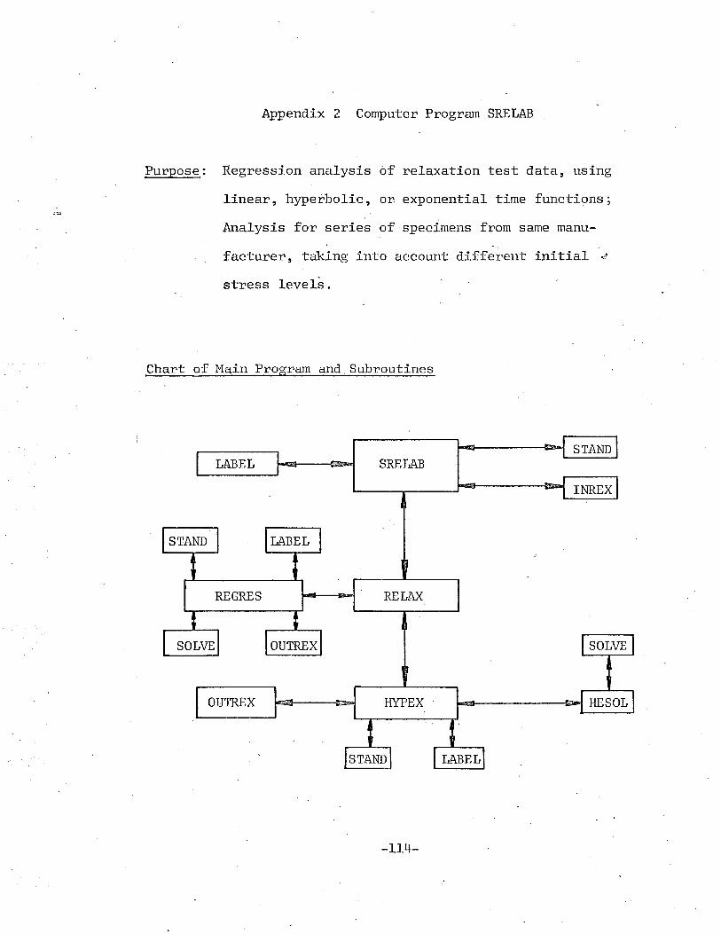
Appendix 2 Computer Program SRELAB
Purpose: Regression analysis of relaxation test data, using
linear, hyperbolic, or exponential time functi~ns;
Analysis fo-r series' of specimens from same manu-, -.
facturer, taking into account different initial ~~
stress levels.
Chart of Main Program and. Subroutines
LABEL
REGRES
OUTREX
SRELAB
-114-

Description
1. PROGRM1 SRELAB:I
Main program for three-dimensional regression of
relaxation test data
2. SUBROUTINE INREX:
Input of relaxati?D test data
3. SUBROUTINE OUTREX:
Output of relaxation test data
4. SUBROUTINE RELAX:
Subprogram for calling of subroutines
5. SUBROUTINE STAND:
Subprogram for estimating fitted data for standard
values of time and initial stress
6. SUBROUTINE REGRES:
Regression subprogram with linear time functions
7 • SUBROUTINE HYPEX:
Regression subprogram with hyperbolic, or exponential
time functions
8 • SUBROUTI'NE HESOL:
Iterative solution of non-linear simultaneous
equations
-115-

9 • SUBROUTINE SOLVE:
Solution of system of simultaneous equations by
Gauss Elimination Method
10 . SUBROUTINE LABEL:
Print of regression function
Input
A. 2 HEADER CARDS FORMAT (lOX, SOH ..... )
Colurnns 11-60 Heading
B. CONTROL CARD
Column
5
FORMAT (515, lOX~ 3FIO.O)
Control Variable (See list of Control ,Variables)
NFUNC
10 NREGR
15 NREJE
20 NOUTP
2S NCOEF
30 NSTAN
41-50 AGMIN
51-60 AGMAX
61-70 FAC
-116-
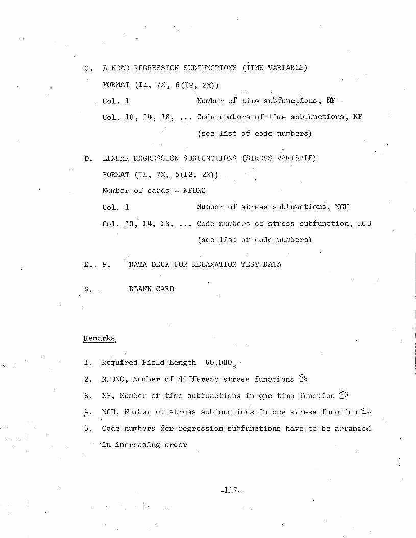
c. LINEAR REGRESSION SUBFUNCTIONS (TIME VARIABLE)
FOID1AT (II, 7X" 6 (I 2 ~ 2X))
Col. 1 Number of time subfunctions, NF .
Col. 10, 14, 18, Code numbers of time subfunctions, KF
(see list'of code numbers)
D. LINEAR REGRESSION SUBFUNCTIONS (STRESS VARIABLE)
FORMAT (II, 7X, 6(12, 2X))
Number of cards = NFUNC
Col. 1 Number of stress subfunctions, NGU
.' Col. 10, 14, 18, ... Code numbers, of stress subfunction, KGU
(see list of code numbers)
E., F.
G. -
Remarks
DATA DECK FOR RELAXATION TEST DATA
BLANK CARD
1. Required Field Length 60,0008
2. NFUNC, Number of different stress functions ~8
3. NF, Number of time subfunctions in one time function ~6
4. NGU, Number of stress subfunctions in one stress function ~l~
5. Code numbers for regression subfunctions have to be arranged
. 'in increasing order
-117-

NFUNC
LIST OF CONTROL VARIABLES
Number of different stress regression functions
NREGR 1 Regression only with linear time function
2 Regression only with linear time function
3 Regression only with expon~ntial time function
NREJE 1 Regr.ession analysis does not include data rejection
2 Regression analysis includes data rejection
NOUTP
NCOEF
NSTAN
1 Complete output
2 Output of origi~al data suppressed
3 Output of original data and residuals suppressed
4 Output of originql data, residuals, and fitted data
suppressed
1 No punched output of regression coefficients
2 Punched output of regression coefficients
1 No output of fitted data for standard values of t and s
2 Output of- fitted data for standard values of t and s
AGMIN· <~AGMIN days
AGMAX
FAC ~
Age of data to be' excluded> AGMAX days
Band-width factor for data rejection
-118-

CODE NUMBERS FOR REGRESSION SUBFUNCTIONS
A. Time Sllbfunctions
1 1
2 t
32
t
43
t
45 t
6 log t
7,1- 2(log t)-
8 /t
9 -te~l
10 t
B • Stress Subfunctions
1 1
2 s f.where s 1
2 =r3 s u
lJ. 83
-119-

LISTING OF PROGRAM
! PROGRA~'1 SRELA8 (INPUT, TAPEt=INPUT ,OUTPUT, TA-PE2=OUTPUr,--PUNCH)C I
~C-~--~T'H~RE'T~:" D-fF1fN'SI-O~N AL ~ANi\LY~S-':fs~~c5F R t~[-A·XA'Tl~oN·"-f~':s'-f--oA TA·~-·~·~·~·
~_~ Y-f~fs.!.~.Q_1~~_~_~J~_~~h~_~~L~_Q~~~~_q__~_~__! __._T..~_t1_~_L._.Alt_Q __~_t!lJ~,~~,_~ __ ._?_IX~~~._~~~ _C REGRESSION ANALYSIS FOR SERIES OF SAME MANUFACTURERC !~-'---'~-C'oM-~r6N/ REl··.AX[3"/sr'R--[8 , 5O-;'2)~~~S-(8-;-SO-;2·)-~;-Sfof~5-;-5-oT;l\F;-K·f·(6~j·i
1 , N G, KG (4) , G ( 4 , 8) ,t\ ( 2 4 , 2 4 ) , 8 (2 It) , f~ ( 2 4) , P T (6 , 4 ); NREG R,-----·2NRE-J-L.-;·-Tfo.0~Tp~-N-St-A ~r;t~:rCO-E~F-~-A-Gf1"tt~r;'-A 'G'H"A'->r;-F-AC-;-N-P~-tJ-f-;~N~s-tG~-~Tf~-f-;'-
3SUM,F8,NFUNC,KGU(8,4),NGU(3)------·----c-b r/fFf5-N7'efD-f- /-"f~-GE --('-8-~--S-o-·)-;t:rA~~--( 8";"5' d~-;'-2-)~-';-~fA:FfE- f-t~-f '-;-F-fN-(-8T~~N--S--;-~j R--·-·--
C0 f'l t·1 0N/ HEA0 / t~ r1 A. ( 2) ,~L'18 ( 2 ) , MMC ( 1 a) ,M M0 ( 4) ,M ME (2 ) , MMF ( 2) ,-,.--1 iVI-F1-G-~-1~i-~fTi~t1-n'[--,-"~i-A-S--;-"i1PT~ -'~~~{ 'A-A -, '~TC-P-;i1--A-G'~--A-G"S--iZ4-'y-;--st'·8 -(--6-'~---- .. ---- ---' ~------.--.-. IN=l .-~~-----.--~----'·f-'6-;~2·"""""""·~·-·-..b~----"""""'~~-~~~"~<·~~+-~··-·-"~-~~".,~~~~--_.~.-~_.-.~........--~~~~ ..-~~,.,---,-,,~ ...............'~'..----.-~~'''-~,-_.~,,'~- '~..............,.--~..-.........-~,,~-, .. ,~~
__, ~__~~t::~?~ .__L __J~_1_=_~~~~_~_ N~_~§_~§~__~_. __ri~~-=_ ..~_2 ~_~.,.__~_~ __. ,.__.__.R-E AD ( IN, 4 0 0 )
_________R..s.BJ~!J,!l:Lt~J!_~_) . , ~_+ ~ . , .• . • ~ ,. , ,~_,,_._
·C READ IN VALUES OF GONTOL VA~IA8lES
REA 0 ( IN, 4 0 2 ) I NF U(\! C , NREG R , NREJ E , 'N 0 UTP , NC,0 E F , NSTAN , ,L\ Gt(l I N---'-~~~~.,~ ~i·'-;:-A-G-f.i"A~X .;-F'-AC~--·-·--,'-~·-~-------~·~ ---~-,.. -.~, -'~'-- ,..-,'----,' --,~.,--,~~.-".~.--~~~"-~.-~"-,~-~-,~~--,'-.-~.~-. -;..~..-----,~ -.-- _-,,"---" -_.-
00 116 M=1,Z-~---+WRI i+'E--(~IO-;-3·-0-0r·--~-·- ~-- ~--.---- -~-- ~---_. __o ~~__ --~--~-. ~-~+----------------
___~_~_&J_T~ __~J,~ ..9_,__~_Q,..Q_! ~ . , .._+_~_ ..__. ~.~__~.~, .... "~_~.~.' .._,, .. ,,_...__.__~,__ .,_..__ ,~._""._
WRITE(IO,301)WR I TE ( 10 , it 01)
-C-~_·~-_~_,_~rWRI=~f''E"~~''~D-E-s''c-R-f'p-f~i-6--N'-'-~O'F-~'-~NAT-·(JR:~·-·'~~6·F~'-~o'"lTfp-ij 'f- '-~~'--~ .~-~ --,- ~-,~-~~-~'-"~~~'--'~--~-' __..~ __.c~",_, -"
C' "AND TYPE OF REGRESSION______~~ .. ,__ ~~__~_~......-----o--~~~ ~ .~~_...........__..~.~~ ~ ,_~.~..-....-......-~~~.~~_~~_~--.....~.......-~ ............... ~ ......~._. ~ .... _........-.....-_......-........~~~__-.....~~.~ .. _~-..-+-
~lRITE(IO,302) AGMINrl R, IT -E ( 10 , 3 03) AGMAx
~-~'---W'R.I'l·-t-(-t -6·~ '3- ij"-4-5-'-t~rFT.fr,j-c--------~~ ,---,----.-,---.~-.--. ----~ ...---------.---,~.-.---" ,._--,--""-GO TO (100,101,102) NREGR
-<-1-·o-6-~--r{RI--T-E~(~i"'o-;-:~f"fi"~'}--"--''--"--~'-------~---~$~---~-~--~-"~~-"~'GO-'-10'-~1-D3~~~ .. "~-_.. _-,--~,,-,--.~-~.-~~~ -~,~ ~.~~ ..101 WRITE(IO,306) $ GO 10 1(3
~IO~rR,-If·E~(-I-6~-'3-[f7)--·----~·-·-·-·-----·--~·-·-~.-----~-._-------~---,_..,.--~---.--~-~.,'103 GO TO (104,.10S) NR.EJE-i-o- it---1TRf -1-E-,{-I-(5'~-3' 'f) '(3-j"'~'-~----~--~-'---'$' ~ ~--. _OJ -_ •.~~ 'G'6--i'o---1 0-6'---'-- -~- ,-_._-;...~-- .. ~,-_.._._-_.- .,----------
1 0:> \'J RI TE ( I 0 , 3 0 9 ) F t~ C .--~'1-0'6~'G~O-- "",.'cy---t·y'o-7--;~itr"8-;i-5-g--;~rI-6)--Nbi]:;(p--'-·--'--~-_..~~~·-~.~-'-'-,~_.-._~-,- ..~~._~~._-,~ ..-~ -.~-_ ..._.. ~. '," -~.~--
107 ~lRITE(IO,310) $ GO 10 111~i+-O·8--wR-tT-t-'(iO-;~-3-i ~lY"--,----------.-. s--~ .-,~-,-,--.·..·---G-6--T·-O~~111-"----~---'--~~~-_·------+-'----
109 WRITE{IO,312) $ GO 10 111--1"1-0-W-R~IT-'t { I (j--,-3-i'j '5----~----------~--~~-~---~--- .. --------~.---~---- ..'-~~--,-.---~----~ - --'-'-'-'-'-"-,"._-+-
-ill GO TO (113,112) NCOEF .---i-i '2-~1rR~t'f~E'rI'6 -~-'3i-4)-4- ,_~~,_~_".",_ ..~.~~O<;'.'~"_~+'~' __ '~'~ ' ~'_~~~~-"--"--',~."--~._-~~~-,---"'-~~ ~~-'-'~ -.'--~ .,"~ ~~"~.. _~., '-'-;
113 GO TO (115,114) NSTAN .-~-[14---~~rR-f'ft (~f-O-,-3--1·5 )---~-"_.~._-'------'---_... ".,---.-,-~--, ..-"'-----._---.--------- ,~-,--.--------._.----. -~- --'
115 WRITECIO,316)--,-- '- -·--··---'·-~4-Ri--f"E-T~t Cf;--3-i--i "--,---,--~-,--.---_.--- ..~. ,-----,---~ -~ .--.._--.---~ .. --.- ---"'~----'--"---'-~-'- -----~-.-. -,-",-~-;
WR I T'[ ( I 0 , 3 1 8 ), '- --- - , - .~_ . -- •._. -.. '_ .. , .." ,""." "_. ,"__,' .. _,~ __ .--..L._~""_._ ~_"''''':''''~~''''''''''''':':'''''-.L-~_'~ _-l'-" __ .._ '---~__ :......... - :- ~.:... , _ ~., .. ~ __ I

116 WRITE(IO,319)IF(NkEGR.NE~l) GO TO 117 , ._~---1..-~__. ..._~.~_~.-..- .....~._ ...__.~_.~_~._
..C READ II'.J NUf~8_ER AND CODE. NUI\~1BERS OF TIME .SUa-FUNCTIONS_~-.B_f:-A~LIN , 4 0 ~_ NF 9 (K F ( I) , 1.= '1 , 6 ) _~__,_'.__ ,_,."_.
117 UO 120 L=1,NFUNC .C READ IN NUMBER AND CODE NUMBERS OF ST~SS SU8FUNCTIONS_. 1 2-G-~R-EA0-rI-N, 4 0 3 )- NGU (L) , (-K:; uC-L-;Mf~, t1 =1 , iZ)~~~-~-.._~,-~--;---_ ...~'-~--.,--,_.~,: '-'~'--'
-- ---_.... - ~ ". - ~..._-- ..- ._- -_.-.~--_._. ,. - - ~~~--~,~.~_ .. ~.~ ...._._-._---~~-_ ........-----..-.~_._-_. __ ..- ~
____C.il1...LlABLl-.L.1JGO TO (119,118) NSTAN
~_1-.1 8 CAL L STAN_D ( 3 -"--)_--+- . ,
. 119 CALL INREX_'~_ILilLS_.__EQ. U) GOT a 15 0
CALL RELAXG_O_IO_._1_.1_3 _
300 FORMAT(1H1,//)-301 FORr'l AT ( I /..:......)~ , -.---~__302 FORl'"JAT (/111,10X,:J.AGE OF READINGS TO BE SKIPPED :: <~,F8ot
. 1,~ OA Y._~~_)_. )303 FORMAT(/,42X,~>~,Fa.1,~ OAYS~)
30_y:_EQ}ltLt1JJ_II/ /, llJ~ JfNUMBER. OF OI_FF ER,ENT STF~ESS REGf5~~,"~SI.QJJ.·~<'
1,* FUN~TIONS :~,I5)
~3J)~LORMAJ_VI / l-,--tP x, *RE:;~{ESS ION WIT H-.JJ NEAF~It~1E_FU N1.J~QtL;?,)(·.)
306 FORMAT(////,10X,~REGRESSIONWITH HYPERBOLIC TIM~~,___1 ~-EllJ1C_T I_O N~~ ) ~~'. _
307 FORMAT(II//,10X,~REGRESSIONWITH EXPONENTIAL !IME~,
_~_,)._~t FUlJCT..I ON:) __308 FORMAT(/,laX,~REGRESSIONANALYSIS DOES NOT INCLUDE DATD~
_. 1 :t- _.Ji~~~~G~lJ OJ'~~::- 0) .__~_~_ . . ~_._._,, ,"_
309 FORr~/\T(/,10X,J;'REGF~ESSIOf\.JANALYSIS INCLUDES OATA'*,_~_~;l JSE_J-EC l_l_.O i't ~_,__:l~OAj_~' BA.tLD - ~..tILLIJLF ~Gl._O R ',t, ::-. , F 7 • 2 )
310 FORMAT(////,10X,,~COMPLETE OUTPUT*)_~ 31~__FQRi~LfLLU_lL_L-L1_Q_XJ ~O_UlpU_LOF ORIGIll&L_IlP, T J~ ~!-)PPR[;_S S.~l}_.~~,).
~12 FORMAT(///J,10X,~OUTPUT OF ORI~INAL DATA AND RESIOUALS~,
_............-_t. J1. S_LJ P R_E SSE 0 :." ) _~ . _._~ .313'FORM~T (////,10X,~OUTPUT OF ORIGINAL DATA, RESIOUALS9~'
1 )l~ ·':A N0 F l IT E0 _JJ~~T_L~U,P RL_~~t;_Q ~ ~
314- FORt~1AT(/,1GX.,J;.PUNCHED OUTPUl OF R,EGRES.SION COEFFIC~E!\lTS~1~'
___________~t-2-.E_QB. HAT ( I--W~_L~OUTf~.L __QL__OAT A F0R~lA~j 0 ~,. RD ,~}. L us.~ 9_f T__~~ )316 FORMAT(I/I/J,10X,~UNI1SOF DATA :~) .
~3JJ EQEJJ f-\J.-J.-l'jJ_J.:-Q_h~J5"~J=- AXAT_1 CUL-~LO~55 : ~ , 5 X1 :,t... FER CEN T 0 FJl',.L _
1'~ INITIAL STRESS';--") , .318 F0 Rr-l AT ( / , 1 0X , -'it T I t~ E :~"., 16 X, ~~ 0 AYS;< ) , . .
~~31-9, FORt/tAT (/0-0X-, ~s IG-~iT;·ux-;~I NITI-AL ST-f~E s·s--7~Dl-T IMAT'-t-~:--;'
........--..-_--.----.--t~t S'TR~SS~)'
400 FORMAT(10X,50H__~~_F 0 :C?~H r~i~-.9_b3~QJj _
. 402 FOJ~t~lAT(6I5,10X,3Fl0.0}
403 ,F 0 RJ1,A T ( I 1 , 7 X , 6 ( I 2 , 2 X) )-~'1--50-'GA. L L--E-X-I-T~'>------~--------~-----'-
END--,-,~.+•• _~-,~~----~~~--.............~.-.-....----.,.........~-~~.............-. .........~~.~--:-~-~ ...............~~~--_._~-~&~---'-~-~.'~- ..-
-121-

SUBROUTI~,JE INREXcC INPUT OF RELAXATION TEST O,LXT'AL
Cor1 M0 NIRELl\ X8 / STR ( 8 t 5 0 , 2) , RES (.3 , 5 0 , 2) , ST 0 ( 8 , S" 0) , t\ F , KF ( 6 )-..-·~_----------.-1._,l:LG_,J{_G_(_itJ__,_G--<Jt.J~ftL~L2itJ_2_'±J--13_l2"~J--,RJ~2~4lJ£lJ_6J_~hNE'LEI; R..J __._~_
2 NRc J E , NO UT P , NS TAN, NCO EF , AGMIN, AGly1 AX , FAC , NP , NT, NS I G, NRE ," 3 Sut't., FB -,__NFJJ~G __,_~G U (8 , 4) , NGU (~3') _~ _
C0 t~J M0 N/ 0 UTI A~E ( 8 , 5 0) ," t~ AR ( 8 , 5 0 , 2) , NAt4 E ( 8) ,F I N (·8) , NS , NR_._~~C 0 11 r1_Qj:L/.H EJ-\ [1 / ~1 t1/\ (~L~ t1 \V1 B ",L21,_ ft1ltQ_t1~Q)~l1i'11)~'±-L,Jv} 1'1 E-.L~L K~'1 E.J__Zl.,_
1 M~~ G, t~l MH , MB L , 1>11 AS,. HPL , MAA , r1 CP ,J1 AG" AGS (. 2 4) , SI G( 6)__~_O_It~tE~~I_Ql2L_k0 A~1lLLL~QfLL8_L--.EJLU~ )
IN=lC:........-_-.,......--;..R E_AlLJ N .NU~1 BE R 0 F S P E C_I~r-..:.....:~E=...;I~~S=--- ~ , ,
REA.O(IN,400) NS___~_~I F--'_~~!_f~Q_t 0) GOT 0 1:3 0
00 1liO I=1,NS '.G~~~~E-<f\,Q_l~_~,L~"fJ-E 0 FSP EC I Mt N--,--_~~jjL I_B ~~llON CO_~ Ffl._Q_Lr; NTS ,~__~~C PERCETPGE OF INITIAL STRESS, AND ULTIMPTE FORCE.Q ~~_-B,~A_O__~lJi~~Jz~~-,~l{[l--;JJ I FF_f; R. ENTl~LE._E A0 I N_G_S _
REA 0 ( IN, 4 0 1 ) NA1'-1 E ( I ) , CO A ( I) ,. COB ( I) ,F I N ( I) , FUL ( I )__R~_A-O t.Ut,-.~!_9~2.l_~ G~~J~~)_,_J:=: 1 ~t NR. E)__~_~ ' _'__~
RE f\ 0 ( IN, 4 0 2 ) ( STR ( I , J , 1.) ~ J= 1 , NRE )!_~1 (] CL_.JsJ:_&D~_lI NJ~Q"2-->__(_S TFLU---,_J..,__2l, J~ tLtL..~_EJ_
:C CALCULATE VALUES OF PERC:NTAGE LOSS~-~=_Q_- .00 104 I=1,NS
_______,~~£~L::~1 __C~ uL_1UN( D~~ FVL ( I )-----:-) --FIN(I)=FIN{I)/100.0GA~COA (I) ~£L__CB:.:COB(I)~FI
___.__-_fjZ_~_=-~.lJ~lL.'-l~ ,:1.) :Jl~_(; A.__~.,__~ ". .......----.--__._BZE=STR(I,1,2)~Ca
~,__~_~-= 1~-..-----~.J "-, :: 0
10 1 J= J + 1 _._~~_"__ ~~ ~ ~~ _I F ( ( ~, GE ( I , J ) e LE • 0 • 0 ) • 0R. (A GE ( I , J) , GT. AGt·1 AX» GOTa 1 0 2
____I.Li~;?~_tI , J_L,-J- T_e A.:; MIN) ~~_I 0 101~ ~.......-
JJ=JJ+l_____ST~lJ_,-~~~~l1 ) =:~X.~--=_~lR (_G~--.! LL~~_g~__
STR(I,JJi2)=eZE-STR(I,J,2)~C8
~~._A G~J.J-,~~.fl= .~ E <_k:JJ_~. ~~_~_~_~~~~~_~ ~ ~__.__~__IF(J.LT.NRE) GO TO 101IF(JJ.GT.NR) NR=JJGO TO 104
__~_~? IE~__'--~_':l. Gl~E:LllP:= JJ_... :.-. ,_~~_~ ~~. . ~_~.~~--_
JJ=JJ+l____~~~D_~~.t_~3 _~ S=J J , NB~.~__.__~__ ~__. ..~ ~ ~_" . ~
103 STR(I,JS,1)=STR(I,JS,,2):::A,GE(I,JS)=O.DI 1U4 CONTINUE.--~.~-~""'-""""-~~~---"""'''--_._'''''-'''''''''~~---_.'''''''''''''''~'''''''''''''''---._~-~-----'''''''''''''''''~-''''''-''---''''''......-.-..-_.-~---~~---.--.-...-............--.~_._-~~-~--_-.....-..-..... .........._-~-~-------_-........-~--~
..~122-

400 FORMATCIZ)___~JJ.~Q __~: {vI ~1__it\~_,~?~~._,4 F1 0 to)
402 FORJ'iAT (SF1'O. 0)__15 O-c-.:R"f:_TiLPJL~ ,_". _
END
-123-

(FIN (1) ,I=I.A,IE)
SUBROUTINE OUTREX (SSS,M)cC OUTPUT OF RELAXATION TEST DATAC _
COM t~1 aNIOU T I ,A GE (8 , 5 0 ) , t1 AR ( 8 , So, 2) , NA~1 E { e) , FIN ( 8) ,N S , NR___---.C-.OJ1l1.0_~1:LJ:iL{J,J)j~M_~_{2.t_,.-~1~L2~1.--'"-M1LC,-(iJU-'_11l1D_(ltJ__,_Ml1EJ_2_t._,J1t1F~t2J--,_ ..
1 MMG , M!'-1 H t ~1 BL , M~ S ~ 1'1 PL, r1 AA , jv1 CP , t./1 A:J , AGS (2 L}) ,.SI G (' 6 )___111JiEJD_IJJJLCL~CLLQ)3_LL,-.kt4-) -----. - _
10=2_~.....-----._DO__1_1L2_-1-~= 1-,li~ _
IA-=L__--.-=1 E=L +3
IF(IE.GT.NS) IE=NS_____~!.R ll.J~_ll.PJ3 O_Q_>_( ~1 AG ,iLflt'l E_( I )-'_I2JJiJ.--:;::;I~E:......::...) _
HRITECIO,301)~__GJLlQ_"11~Q_g_1_J_Q2) i'fl_~
100 00 101 J=1,NR...=:,.C__....-O UTPUT 0 F 0 ~~. I GIN AL O_Al1u-~_Lf IT T_EO~~11LE_~.~~L 0 S_S-c- _
1 0 1 WR, I TE ( I~0 , 3 0 2 ) ( AGE( I , J) ,S SS ( I , ,j ,.1) , I = I A. , IE)~_.._~~ __lQ~~L __.__~
102 DO 103 J=1,NR~c~ ou"toPUT__Q.L RES 19J1~~L S
1 0 3 \.~ R I T E ( I 0 , 3 0 3 ) ( 1\ 'J E ( I , J) , (S S S ( I , J , K) ,t1A f? ( I , J , K) , K::: 1 , 2)
----.----_-J~,J~=l1u_J__E )104 WRITE(rO,304)105 CONTINUE____ ........~~----.-_--+--4""'"~....... ---r- ......... __3GO FORMAT(///I/,3X,4(4X,A3,9X,A4,10X)3 01-~QJ?~ rcl.L\lJLJ ~~ ;
,3D 2 FOR r1 P. T ( 3 X t, 4 ( F 7 • 2 , F 1 3 • 3 , 1 0 X) ),i~:? 03 FOR 1"1 ALU_~'_~LLEL.~__?_, F g • 3 , A1 1_F B ._~__t~t-, It X) )_~__~~~~~__.~~
394 FORMAT(II,7X,~SIG : ~,F1G.3,3F30.3)
.__~__._~fl~_T1JJ~~NEND
-124-

SUBROUTINE RELAXk- _C SUuPf(OGRAi'1 FOR CALLING OF SUBROUTINESC
_~,__J
c0 i~ ~1 0 r~ / REl AX8 / ST R ( 8 , 5 0 , 2) ,R ES ( a , :; 0 , 2) , ST0 (8 , 5 0) ,t\ F , KF ( 6 ) j
_~~__1_Jl-!_G-!~~~G~._t-,-4:.1_t"_G_C~tJ~8), A( 2J±_!L2~ltl~~9-1Z.~ __uRJ_2_~J_._,_f~LL6J __~_u_Nl?~EJiP~~.. :2 NREJ,E, NO UT P , NS TAN, NC aEF, A·GM IN, t\ GMAX , FA C, NP, t~ T , NS I G ,N RE ,
__~S l}J.L£fu NF U{\.1 C, KG_LLL8_L~tLtJ~L~JJ ( 8....:..--.)__~ __CO HMONIOU T / AGE ( 8 , SO) , tvl AR ('8 , 5 0 , 2) ,N ~ ~l E ( 8 ) , FIN ( 8 ) , NS , NR
_-C-'----O-'-N MQ~l! HE AI21~tttt~tn-'-.t1tl ft{_Z~LJ_l1 ~1 G~!1J~tL,JitLD~~_, tv] ttE~..l, Mf'1c_l£L,~ .1 Mr'1 G, ~i MH, r1 8 L , f~t AS I) j i"1 PL , 1"1 AA , MCP , t·,,} -A G, AGS { 24) , SI G( 6 )
~ J0 =2 ~.-_
GO TO (101,102,102,102) NOUTP._1 O_LW R1_1E_lr~~L~ t\ ~1 E UL~t:=_l , NS)
WRITECIO,301) M
_~__~:LJ10 I ~ 1_, f........:.....\l.;=....S~_
00 ieo J=i,NR_~__~lliL-lQ.~=l~,~...:..-P-,--_-..--
100 MAR(I,J,K)=MBL_______C..8J-_~__ 0 tj TP~_liS T_R ,_(l__.. - __~--.__..-------. .....--__._
102 CONTINUE~ ,JJ_L1.1Q_.J1=_t , NFU_N~C_~
00 104 I:::i,NSDO 104 J=1,NR00 1 G4 K= 1 , NP
_10.~.--l'IA RQd, K) = tvJBLDO 105 L=i,NG
.............--~__~H~=N_~1JJJ~ )1 0 5 KG'( L ) =KG U ( N , l ) ,
~~~_~E (NR~GR c ~LE~~Q--lP 10 3CALL REGf~ES
____-.-_~_Q_lQ-.-:L_O--6_-.--....__--.-.-----_... '---'-~~ --.-.----..--__. .....-.--.~...- ._#.
103 CALL HYPEX106 CONTINUE
-~300~:-0 ~MAT { 1-}-11-.,~/-/~,~7~X~.-;·"-~s' ERIE S J~~ , 8 (5 X, A4 ).-}-~~--.-~----~----
~3 O_L~_tO&tL~:r~( / / ~~7 X,~~o RI :;1J~L OA ~~l-_~~ _150 RETUf~N
END--
-125-

'SUBROUTINE STAND (11R)
cC FITTED DATA FOR STANDARD VALUES OF lIMlC. ~~~l 0 I l'J lillL S TR E S_S"-L- _C , ,_.~_C_Oill1.D_~LEZEl_A.XllL_S_t_R.~(JL,.5~__'_2_hB E:L(J3_,_2D_,--2)--,_SlQ1B.~,~f.ll_,.1~LE,J~£J_EU_1
1 t NG, KG ( 4 ) " G ( 4 , 8) 1 A (,2 4 , 2 4) , 3 (2 4) ,R, ( 24) , RT ( 6 , 4) ., NREG R,_~2=-:::~Ji[ J E-,~LCLUE , NSTAN JJiC0Ef~Gt1 IN.! A~~ MAX, F ACLNYJJ'~ T ,_~! ~ , f\1R~
3SUM.FB,NFUNC~KGU(8,4),NGU(8)
___~_GOM.t10J~t/Q_.UT/ AGE (8 ? S 0_> irl ARl_~ 5IL.J_ZJ__,_,~A~·1E lll1-F_LNJltL,lLS_Ltl.K__C0 H ~1 0N/ HEA'0 I Mr1 A ( 2 ) , ~l t·1 B ( 2 ) ,M MC (1 0 ) , ~~ t~~O ( 4) , l"1 ME ( 2) , f~ MF( 2) ,
__~1MkLyJJjJ1tL, j"18 L , ~1 AS, M.P LJ J1 AA , til CPJJ~L6J.. 0_S_( 24 ),--,-S1_; (6 )DIMENSION"E(10,24) ,H(4,6) ,SST (-24,6) ,T(4,6J
__......---::1_0=2GO TO (11?-,1fJ5,114) HR·
_r--i_t~I Fi.tJ PE_~iE?~_JL~LE-L1_~)~~Q~_LL~Q_2~~__._~_ __~------:---
C GENERATE VALUES OF TIME SUGFUNCTIONS FOR STANDARD TIME,_~_D~1L.Q_~_:::~Li11_
·E(1,I)==1.0_~__. ~~J_.g_LJ.) =A2~lJL ~_._~
E(3,I)=AGS(I)~AGS(I)
~~_.E-:{.~J~-= AG~-.Il!.J~ ( 3-LI j _. E(S,I)::t::(3,I)~E(3,I)
~---:E ( 61-l)_= (1, t. Q.G 1 Q~V~S ( I l)E(7,I)=E{6,I}~E(6,I)
_----.:E==-(~I):::SQRT(AGS(I))E(9,IJ=EXP(-AGS(I»
-.-J_Q_Q~tjLt_ll_=1~Qj~; ~_ill__ _C SORT TIME SUBFUNCTIONS ACCORDING TO INPUT CODE NUMBERS M
__~_~QQ_)Gl K=l,NFKK=KF(K)
__-__~l_QJ.~ J =:LtlJ_T~_--..-..--._. --.--._____..E(K,I)=E<KK,I)
__1 0 1~(; 0 NT I NU~E _~~~ ~~~_-.----.--- ~'__C GENERATE VALUES OF STRESS SU3FUNCTIONSC FOR STANDARD VALUES OF INITIAL STRESS
-~----
102 DO 103 J=l,NSIGH(1,J)=1,OH(Z,J)=SIG(J)
_._~ ~ ( :tL~) =_~_!'G (J )_~c.?-.J_~_ (_~J~) ~. _
103 H(4,J)=H(3,J)¥SIG(J)____~_Ci9._T_P 15 0_'~~.
115 CONTINUE \L~_~ORT_. ST~zE·SS SUBFUNCTIONS ACCORDING TO INOUT CODE NUHBERS·
00 104 L=1,NG~_~~~~~L=KGL~}_ _'~_
o0 1 0 4· J =1 , NS I G____~_" ._~_~ __ t~_-,-_~2 __=H~~h_J _J~_~ , .
~04 CONTINUE~ ~._~Ji~RP_I+r;_£tIT EP_~A~J} Es__~~ NG~~_~.A FG__.H YP~E RB0 L~~ ~_
.C OR EXPONENTIAL FUNCTIONS
-126-

_J 0' ~ ~Q,_T_Q JJ~:_,~Q __,~~ __QJJ_t1:1JJ )__NB E~ R_,~__1G6 DO 107 I=i,NT
00 1L7 J=l,NSIG--·-------'-·-SS.T-('-i--;··J-f;-o--:-(f'·-~'---·-~-----~~~--.--~~--------~-~"---~-------"-.._-,~~.-_____-__00 107 K=i,NF
o0 1 0 7'- L =1 , NG__ ." . o...--.r-~. ~,...~ _.~ a_ -+---':':"_"._+-
_.1-n2__,.~S_S_I-lLs_JJ--=LLK_,.~_~ILL,_J_)2J{~~L,_(j{_,_LJ_LS.s3~!L-J,~) - _____GO· TO 112
~.Jl.~a~._D~CL~1_0__9_~J~.= L ....}tl__, ~_~~'. ..~...=~ __
BA=AGS(I)/(F8+AGS(I)}__, -.l)D--LQ9~~'--_~LSlS~
SS1(I,J)=O.O,~~........D~O 1JL9__L_=..L,~LG~ __109 SST (I,J)=T (L,J) 1t'-R(,"L)~t8A+SST(I,J)
_< -~.ii_O__ID_E.r~1.-i-2.~_~------. ~. ~,_ ....,~~110 001:1.1 I=i,NT
______B.A.:= AG.-S-tJ ) J;. },.t F,8::...-- _00 111 J= 1 , ~.,! S I G _
__~----S-S_T-UJ_J-J-=0_,-__0__._-------00 111 L=i,NG
_~__4~11- S SLtL,~\.~tl~= T -!~~,1._~JJ~~ ~_l_s.. ) ~{.lt&±-.:$5-l-1l.L:LL,~__~_..;..........~..~,~,~~ ...=--....."-~~'_,"--"""~~~~~. 11 2 ¥J RI TE ( I 0 , 3 0 0) t·j f"i A ( [1} R) ,~1HB ( f1 R )
Wf~Iit_0~J 3 0 11- ' ~.---'_~_.00 113 I=i,NT
_ti_:~_W_E~I~_E_J_I_CLL3Q2 ) AGSJ1_l-,--~S L_{_L_~Jl,__J~=:.1_, NSl_~_~_._. 0__• __
WR.ITE(IO.3D3.> (SIG(I) ,I=1,NSIG) 0
~~3JllL.~._EJ1~J~L[tUi-L_L-,_-7 .~_". ;t,f_rJ~T Eo~_."JJi\lJj~__f=-QR~<~J· A~LQB_R1: ~.8~1l.E_~....J2.£_,__,I-,_~&t!Q~_t,1,~ SIG~,10X,2Al0,1/)
_~~O_1. __FOJsl:1 A, T l11L~~(; E* , =' (_9 X , 1:;' LOS S-'I- ) ,_U-)_______________ ,~~_3D2 FORHI\T(F,10.1,6F13.3)
_~~_O_3..-.E..QR MA_L<_/ / 1J XJ . :/0 S[JL.J._~_,.L1-.1_~3_., :5 F 1 3 .3-L__~ ..... _I 150 RETURN__--~_~~~f;:~N~Q-_~~_,~---:_~_r .~,'~_~_'_~'~'~'_~ __~~~'_~O'-.>~~ __O<_~ ~ ' ~= .....=~~~_-'"=._...=~""-"~~~.'. _~'~.
-127-

- SUBROUTINE REGRE~
_C~ ~~~- ~. ..:__...........~_~.__~__._._.~ ...~_~ .~.,.._~..~~,_.......-.....--_eREG'R ESSION SUB P~~. 0 GRA1,1 (R EL AXATION TEST 0 ATA)
'-C-__--LillUR-T-.l.t:1L-E1LtLlk-UQtlSC
___~__1'&t11~_Q~LLB~_E~~_~_8LSIiLJJ3J3JL,_2_1--,_RLS ( HL2JL,-2h~TJU_<lJ3_Ql-,~~E_,_JSL ( 6 )1-,
1 ., NG , KG ( it) ,G ( it , 8) ,A ( 2 4 , 2 4) ,8 (2 4) ,R ( 2 4) , f? J ( 6 , 4) , NREG R ,_.~~_.__2JlliE~J~E_i_N~O_\:LTP ,j\:ti]~.llJij.-tLC_~.~f_, I\J2J1~IJ'.lj~_G (11\ X ,_FA~J__tJf~,_NL1'lS- I G1 NR E~-,_~__
3 SU11 , FB , NFUN C , K GU (8 .. 4) ,t-J GU ( a)___,_C_llirl MO_t-l/_QJJ~LaG~E_J13_L2JLL,_HA~L8-,_2.Q_~_2J._,k~A~l E:JJil~L:(l'Ltt1l-,__NS--,_tiL _
C0 t1 fvI 0 t'f I HEA0 I 1'-'1 iv' A' ( 2) , ~1 t··18 (2) ,r1 ~1 C( 1 0 ) , Mt1 [) { 4) , M;'·1 E ( 2) , MMF{ 2) ,_____---1~_t::lCL.,Jititl_LtlB_l~MAS, MP L-,j1AA-1l1C~-,_t1AG_-!,M2.S~_2~-, S I'G.~{---.0:;:.....6.;..........) ~~
DIMENSION F(10,B,SO)_.~ ~~~1_9-=_'~~
MR=1 ,__~__,t-ltl~fL~-S.__
DO 103 I=1,NS___ ~ D_LLQ2_J;: L-! NR . _
C GENERATE TIME SUBFUNCTIONS USING ACTUAL TIME ARGUMENTS_~~,,~_~,~,~_~If~tAJiEJ_.b-,~~)~ll~E ...~Q_).._~Q_I~~~_CL_.~~ ~~._"-'--"--"'-"-_~_"~' --:'~~",,-_~_~~,""-_~~' __.,_
F(1,I,J}=1.0__-_'_~£l~I_,_.-J] =_~_f~Ll.-,~J , _
F(~,ItJ)=AGE(I,J)~AGE(I"J)
\ ~._f__~t~IJ-J-L= AG£_LI-!_JJ_.2:f_t3--,_L1_~L2. ...__. ._F{5,I,J)=F(3,I,J}~F(3,I,J)
---._==--~.~.__£ ..t.9_LJ,,,~JJ_==F1_1_QJ}_.1~JLJ~:~C2 ..r;~U~,,~~ __t~_~~~, ._~~.~,,~-~~_~.o><=~ ....._"~.. ~~_~L~~"""-'--"'~_'_"""F(7,I,J)=F(6,I,J)~F(G,I,J)
F ( CiJ_1J_J) =SQRT ( AGE (L_~.LL _F(9,I,J)~EXP (-AGE(I,J»
__~cJl~L-,__~~L) :::_-L~LP GE:l.LLJ }GO TO 102 .
_..........-."",,=-,1~U_U_CDJJ~,I N!l£ · _~_.._~_.~_~~_~~._~~_~-._~......,...._~. ~_........_~.~__. ~ .._~~.~_ .......__DO 101 L=i,10
1 0 1 F ( L__,_:Lt_.~L=-D_. _0 _102 CONTINUe
_L~---.-JiE N Ef~A T_E-3~ L u£_2-_~__ STfiE. ~_~_s U~_E'Jl.!:J CTIp NS _C FOR 1\ CTUf\ LIN I TI AL S TRES S ~ VALU'c s
.-.-=._~ ,~~_,L1.1~L!._=~-.~~Q,~=,~.~"........,."..,.,. ..~~~-......._~.,_-=-='.,~.~~~~~ .._.~ ~....-....-.-_' .-....-..~.... ~...........- _G{Z,I)=FIN{I)
, ~G_J~_.!_12 =f_I~ ( I ) :~{ FJJiJI1 _,G(4,I)=G (3 ,I)Ji.FINCI)
.__tiJ~1.-_G..9_tlllJ:~L~,c ,_.~. . ._._~_~.__~._~~ ~ ._.~._O~._~ ~__. _
C SORT TIME SUBFUNCTIONS ACCO~DING TO INFUT CODE NUMBERS. .~..,__~,.._J2~Q~ __1.Q.__l.A-~. ~~.=~1-.,,1:.LE~~~<",_,=--~.. ~-c= .-==--">.=~......~ .....="*"'==-.=-<--='==-._"-~~~.,,~~........._,...,..~~~' .~.~->- ..._"""",-__-_'~..................~~~~_~.
KK=KF(K) ._ ..........~__._OQ,-1JL~__JcJ_-'-_N ~ .
DO 1G4 J=i,NR ,__i._P~F '< Kl_L_JJ :.:: E-(_l<;.~, __I , ,lL ,__.~._. ~ ~ ~_· ~--- ._.__._.__.~ j.
c so R'T STRES S SUB FUN CT I ON SAC CORDI NG TO I NPUT CO 0 E NU:~18 ERS____~. ._-~,Q __..tiL2~=1.~~_~~~_,~~~ ..~_._~~~~~. __."...'".,~- .'~~r~t.'=__='.-·__..~ ..__•__ ........,.~O.._""~._J~. ._...... ~'~.~ .____=.~~~ ,_••~ • ..-<>~_~~
-1.28-

-_._~----
..........
lL=KG(L)_~~ JLQ__ 1 GS J: =1 , ~~ S
105 G(L,I)=G(LL,I)_.~__~_i?~ ~t~RA T.E __S_Y ST_c ~1 ,~£__SI ~1U L_l~N EqUS [QU AT ION S
NF G=: NF~''.. N~
___~_2~O~LJ]~Q~,J.~CL..tL__l:: =1 , NF~B(L)=O.O
___-..---.-.-.----OO.~Q6.--t1=-1_,01E~
1 tJ 6 A ( L , ~1) =0 • 0__~-----"SNOI\1:=D--LO__. ~__............... _______._..~ ~,
DO 108 I=l,NS~ O_O__lj]_fLJ~_,_~R
DO 108 K=i,NP_____I"--'-.-F---...:("--.-.,;C"'-'""'S TLLLt-JJKL.£lL.Jl__~t..QL---.O~-.Ll1AE_LI--,_J_-,J~1 __~M5_U---CiQ._LQ __i.D....a
SNOM=SNOM+1.0___--=00 107 L~=kN,.....:......F ~__
00107 f71=i,NG____JA,y_= ( L- ~) ~ NG+H _~~ _
8(NV)=STR(I,JtK)~F(L1I,J)·G(M,I)+8(NV)
_.~_~P_J-P_'L-l- H:: 1-,~£ _00 107 ~1H=1,NG
NH= (LH-1) JfNG+~1H
107 A(~,JV,NH)=F (L, I, J) ~tG (l"i, I):::--F (LH, I ,J) ::~G(jvJH, I) +A (NV ,NH)108 CONTINUE ~_~
CALL SOLVE{A,,8,R,NFG)_~----.:.vlli._r_J_E( 1.0..-, 3 CG) MMA ( t1 ~--' r1 H8 ( MR) , N)!dVl E (1 ) , NAM§~ (N S)
CALL LA8EL(2)_.....-- JiR.I Tt;fl~! 3'0 1)_~_~ _
o0 1.0 9 I =1 , f\l F_~~D: O~l~G_~~:;: 1~G
NV={I-l):'~NG+J
~~:LlL9~Rl~U_~J) =R {NV>DO 110 I=l,NF
11 0 ~i RI T E ( 10 , 3 0 2 ) ( MAA,I ,J , RT{ I , J) ,J=~ ,NG ).GO TO (113,111) 'NCOEF
~_.1_1_1_~!J~~C_H-2__CLU-,~~t:ttt&JJ~1 RL_tl1_~,llitl RlJ-.1LLitiE (_tJ-,_.~lA t1 [ ( NS)00 112 I=1,NF
_L~_~_Gl:Ji.f~J~Al~--L~_I_I_~LYB1JJ~~f~QS_)~__+ • ~ ~_--__-~-..~----112 PUNCH 5Jl, (RT(I,J),J=l,NG) '.
__~~_~__p~1J~~r =1 ,Ji~ .~...._.__.____ _~.---.....-_' ~_, .......----_....-,__~__.. DO 114 J=i,NR
S Ta (I , J )- = 0to·-----~~DO-11-4-C:::1 , NF--~--------'----~......-~---..----~-~..
~_~~__Q~--1_14_--l'1=_!_J_N.G "114 STO(I,J)=F(L,I~J)~G(M,I)~RT{L,M)+STO{I,J)
______~o TO (liS,11S,11~,116) NO_U_T_P ,. 1'1 5 ~J RI TE ( I 0 , 3 04 ) t71r'1 A ( MR) ,t'l r1 8 (;'1R )
_~__~_g_~~~~~.Qj2.IRE x~~.l0 , 1)_.~ ~_.. . ~
C 'CALCULATE RESIOU,Al..:S, SU~1 OF SQUQr.zES, AND STAr~OARO EF~ROR
116 SUH=J.O-"~--~--~--~---------------~---,-~-~-_--~ -~, ~,,,_. .~_. . ._. ._J__
-129-

.J
-----.._---------_._----------~---~
DO 117 I=l,NS___~Q~i~_~_=:_~ , NR
DO 117 K=1,NP_______[{_~~_(_I , ~ , K) -= 0 • 0 ~~__~_~_~_. ~__
I F (S TR (I ,J , K ) • f\l E • u• 0) R. ES' (I , J ~ K). =SlR ( I, J, K) - S T 0 ( I , J)
_~~~I_fJ_Mt.tE'~_L~~,-.~_~_>__ !._~.Q._~~j J1~1__ GOT 0 117_~~SU11 =: F~E S ( I , J , K) -to!. RES ( I ,J , K ) +SUf1
__1~~~~l~.NUESTO~SQRT (SU~1/SNO~I) ,
____.WRI TE ( I a , 3 G.2J__!'Lt1Al i-1 R.) , MNJ3 tt1 t\J_-!5 N0tj ~ ~_~_._
WRI T E ( I 0 , 3 0 6 ) Hjv1.A ( r'1 R) , rl N-8 ( r1 R) ,S Ut~l ~
~1 RI TE ( I 0 , 3 0 7 ) ~1t1 A ( r1R) , ~1 H8 ( ~I R) ,S T0---------(;0-1 O---(,i-1-9-~-i1 B-)--~Js TAN~---~-···_----·---------···-·-~~-·--
118 CALL STA ~1 0 ( f1 R)C REJECTION PHASE
---1-1-'-L--C-R-~£AC!t.S-r-D-,~----_._--
00 120 I=1,NS__~~~ Qg_-1_ZJJ__J = 1 ,N~~f<__,
00 120 K=i,NP___' I£LU12_S_{RE_S_UiJ--,~KllL-L£=-!_C Rll...~R~A R._(J_.l~,~l~£Q 0 N_JlSJ L__'
1:';0 TO 12G__' .!-...!-M.Af?,jJJ_J_,_Kl_=-r1l1K__.~ _120 CONTINUE
_ ...... ~_-=-............£_O--1J)~.J--1.2J~_~ __12_t--,-L22.JJ2.2_) JiQuT-E__. ..,....".~. ............-~_~__.__~_-__~~~~ ~
1 2 1 ~~ R. I TE ( I 0, 3 08 ) r"1 t·-, A ( tIl R) ,~1 r1 B ( 1'1 R)____,_-.-C AL_L-iLU1J:~"E~ (R E_~-1_21. _
122 GO TO (150,123) NREJE___-12~3_JiO~_O_J_12h15~D_L.....:.._=_~1 ",----,--F: _
124 ~IR=2
-...- ~~_~M t1K :::~~jl?j~-_.-= __~~GO T,O 20 0
__._3_0_u_-.£_O_RMtLLt1 H1_JL, 7 X , ~(. _L E ,n. S T SiLU ,n RES FIT 1(. , 9x-'- 2 A~.JL,_1J2~ _~~SP[CIMENS~,2X,A4,* •••• ~,A4) .
__3_0..1-E.OJ~lvlt\ U_/1.LLJ_lXJ-~i?~£ F< E2~lStbL~C_Q.E FEI_~tJJ~~T~~_t_) _302 FORMAT(7X,4(A1,I2,I1,~= ~,E14.5,10X»
_~_~_~._O~_3~,E~Q~fS..t1AJ~=tl.x..,~'i ..t-,_IL,~ =~,~~~~ ...!±~~.~9~"L~~~ .~ ~~.~__~-_<-,-",,,-,-~· ~,"-.~, ~.. ....,.'-='~-~~.
304 FORMAT(/////,7X,~FITTEOOATA~,5X,2A10) .3 G5 FOR t~'l r~T (/ LL-,J~_1~~{J)r'18 f; R a_F D ~ T A :;.--,--Zl:.J_Q_1 J:.. : ~t ,£~~~1L., / ), _3 0 6 FOR t1 AT (7 X , ::~ SUf1 0 F SGUA, RES :;. , 2 A1 0 , :; :: ~;. , E1 2 II it , I )
__. --~Q-7_-.-EiL~.tttl.LJ.L_~j_:~S TANIJ-!.~B. 0 ERR 0 R ~t , 2 At~QJ~: ~-Lf l_~~J_~__. _308 FORMAT(/I//,7X,~RESIOUALS ·,2Al0) .
, . 5D 0 Fa Rt~1 AT (~RE GR'f, SSI ON COE FF Ie lENT SJ}. 5X, 2 A10 ,10 X,____---...-....~~_._~".~".~..,.__. .__~._~. -.__,._ -.--~_ ,. __~_.__~_~~_.._~. ~~~~_.~ __..!__.~~-_._r_~_....___. •.~~~ ..............."·~____..o=_-__~~--""'_=---.h__~=--
, 1~SPEClfilENS:.l,2X,A4,:tI- - >;.,.A.4)S01 FORMAT(4E14.S)150 RETUK'.N
___..~ EN0 ~__._..,-- _
-130-

-'---~""l
SUBROUTINE HYPEX. -...-C~ .........-.--.. ~-__~~~__~. ._.~ "~_,_, --..-------,.........._~_,,,,__~--...,~ ~,--
C REGRESSION SUS'PROGRAM (RELAXATION TEST DATA)--C .ti.Y_2J~J?IiD_llC_-iLt'1~-LXEJ)Nc tiI1J\_L,E£ GR~ SSIO·N ,. I ME FUN CT ION S . .. C ._'_~ C_OJitJ._OJ.i/_R ~ LAXJ3.LS._IP~~Bj2.o-,-,_2.L, RE.s_l3.J~2Jl-,_2~ , S I 0 ( dj.2JJl1,_~.f~f.J~1_
1 , NG, KG ( 4) , G ( 4 , 8) , A ( 2 4 , 2 L,,) , 8 (2 4) ,R ( 24) , RT (6 , 4) , NREG R,_--............~.__._21:1.RLJ£=-,.1'LQJIJ PJ NS~Jl._,-rJ-.CSLE.E.,l'j; M_ltL AJ~ f1 AX , F AC, N,p.,_H.L_li.SJ~GJl! RE J_-=
3SUM, F8,NFUNC,KGU (8,Lt ) ,NGU(8) .___----C_Q_11 t-'1 Ql~LL_O UTI~ 0 E..l1tj S v_LJJ1 Afil:~.2Sl,_Z) , N fJ t1 E ( .8 >.-,_[1 N_{ 8 )~~..JlJR-~_~
c a 1'1 t·j 0 N/ HE A0 / ~ i1A '( 2) , ~'li"1 [3 ( 2) , r·1 ~1 C ( 1 0) , t·l p/i 0 ( it) ,rH1 E ( 2) , M1~1 F ( 2) ,____.1~lrlG, ti MJi.,J1IlbJli~ MPL , HAA,~1C.EJ t~f A~j~,li.SJ~2 4lJ__SI G-L9l- _
10=2__C~~~ ~f;_N ER~.AT.~_'""~~~s TRES S $U 8FU NCT~J ON S. .-..
DO, lCG I=1,NS__--=G tL_J._L= 1_t_fL _
G(Z,I)=FINCI)___---'---_G~(_3._,._I.L~£I~_LI ) ~t .EIJi.(_;:Ll.
100 G(4,I)=G{3,I)~FIN(I)
-:.rLc,.-.~~."~.,_.~_.S.O.RI.~_.JS>IJs.f~~i.S_.5_UBJ~hLN C'~Il__Q_~~ ~~ ..._00 lot L=i,NGL.t-_:=K2J L)
DO 101I=1,NS~ .J.l~_1-_G_<-_LLI_L-=-G-.t.L_L-,_I-l · ~ . _
NL=1~._,~~_~~_.!£"Jll.E.t_2R.~£~·_l1..._~ ..l;.~=~L~ __~__~=_=_ ~~_.~~~~ .....-~ .~.~-~==--""~-_"'=~.,~_~=--~.~_""-"'-'-'__
t1 r~ =1. iY1 t1 K=: ~'1 AS
200 CALL HESOL(NL)____ Gfl__I.[LiJ- 0 2- ,~t_O S1_-.J\1 L _
1 0 2 ri RI T [ ( I 0 , 3 0 0 ) f~1 i\1 A ( t1 R) ,- f-'U-1 B (~1 R) " NAr1 E ( 1) , NAr1 E ( NS)~L~~_.c__~~_~ ..rLU~j~_T_E_._ .._,E:r_.I T E~Q.__VA~b1LE~~_.JJ£~b_~Q_~~~~'iJ..tlli_~~ ~.~.~___..~""".,_~~~~~-__~~_~~"_
c · HYPEF~80LIC OR EXPONENTIAL Expr~ESSIONS
o0 _~_Q..L 1:=1~S- __SAS=O.C .
. __1l..9_12 O__l-::J.~_G~.~_120 SAS=G(L,I)~R(L)+SAS
_..~~~~~".~~- ...~'"=Q~Q~~ ..~_"Q~~~J.=.~-~L~B~=~=~ __~~~~__~~...-.......-'_~~_.-.-_. ~__-....-.............---.._.~.~ __. __._~~103 STO{I,J)=SAS~AGE{I,J)/(F8+AGE(I,J»)
_________CAL_~M_~l~ 2)~__~_GO TO 108
____--~jJ-2_- r4RJ..T_EJ_I tL,.~~Q.1_!._ M~1 A-.Uif~JJ:Lt1_fl_( t~ R}_1_NA_ME~11LN A~.£!. Ns)__~_~~~__T
00 107 ~=l,NS
. __-_._-.__~~~85.:~Q~~.~ G. ~_"_,=~._.......'~_~,=n...._.". .=--~~_=____~"""'~_._=~., __~:
. 00. 106 L=l, NG__,.__1-iL~_~.A s.=;;_ ("L. tn_)" R (Ll.±~.i\~__.
oa 1 0 7 J = 1 , ("t R::.....__~:t_OJ~S T_~lL_~J =_~A~:;' AG.f~~.J_~l:_~_E.£~ ~____ _
. CALL LA8EL{Z)108 WRITE(IO~302) ,
~ .........-.lo.~:_--.; .........:..~--: ':-- ~ .. ---~ .....---.....,..-.~ ..._.__: ..,;.........._.~--;--...-..........--- ... - ...-~---':::I!.-:L.j.~... -. ~n·.:"...,..~:c:r_~'L...~-.~~"""'IL7"~..r:.:.l:...~ .. -·· .. ........:_....~·~;:_~~..~ ...................~_~~..-.:~~~~.__.~.~~~~.....~.- .~'LJ-w.::..II...~.'1.,I. ..............
..·131-
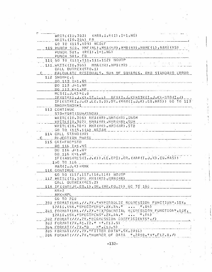
----------~' --'-.---.---.------..-~-
c
r --.----,--~
WRITt: ( I a , 3 a3 ) .( j'1 AA, I ,R ( I) , I:= 1 , NG)____-.JiE-I Tt:flQ_,-_3 O_~E.lL- ,
GO TO (11.0,109) NCOEF ,.__1 C9 __EJ) NCH~~2-0 Q_,__~~LM F {NL~~t!tt A,( _t!!lLLMM8 ( M~_~~~1 Ei ..~l:l_~_M E (~~-.:_'
PUNCH,501, (R(!) ,I:=1,NG)___ p UJ:l.Q..tL2~h~, F ~
110 GO TO (111,111,111,112) NOUTP--- --" ---,.,~--.. ~,- - - - -~_ ... _.~- -- - ~-- _. - .. ~ ~
__-1-L1._-WRrJ_E_LI_O-,_.3J15l~li:1R~)_,J11:1B_J.-l'1RJ __~__----..-.:.....C~LL OUTREX(STO,1)
-...-::'t:C~_~CAl-~CJLl-ATE RESIDUALS, SUt·l OF SQUARES, Al'!D STANDARD ERROR112 SNOrvl=O. 0
_________-~_{lO_1-L3~--LJls_--'--_00 113 J=1,NR
____·D_QJ__l+~Li{.=-L~ pR·ES (I,J,K) =0.0
,__---==1 F ( S T P~I_,_J_'..K.0_G T • eL. U) R~ciJ_L_J-,~K l =:-S TR ( hJJ..K) :-_~IQl-L",-.JL__I F ( ( S T R·( I , \oj , K) •,l E • 0 • 0 ) • 0 R. (M l~ f~ ( I , j , K) tEO. • ~1 AS) 'G 0 T0 11 3
______~~1iO t'1=.S_N 0 ["1 +t ~ ~~____ _~ _113 C0 f\l TIN UE
~~_~'_~~]_(J-=-_S.Q R, T-1 SUM I SNO f-·1') ..~__- ~~
WRI T E ( I 0 , 3 0 6 ) t~1 MA ( NR) ,ll t1 0 ( MR) ,S Na t'1________~~R+LTf~_UL, 3 0 7 ) t'i MA( i'1 R}_tl1t18_(JjJ~D5_l}lL- _
WF( I TE ( I 0 , 3 0 8) Mfv1 A (N R) , t'1 i'1 8 (1'1 R) ,S T0___----:c,=-....;... (=-)_1...=.-....=-0~(115 ,_1_1 ,4) NST~N
114 CALL STANO(MR)_-------------'"REJECT~ON PHASE115_ CRI=FAC:~STD
__.__~_.Q~~LJ1-_9_J:=:1.__,~__00 116 J=i,NR
_~~~o0 11.t?_~=J--, N,P _I F ( ( ABS ( R. E S ( I , J , K) ) • LE • CRI) • 0 R. {1'1 AR (I , J , K) • EQ• NAS) )
1~O TO 116MAR(I,J, K) =Mt'1K
116 CONT :t.NUE _~__GO TO (117,117,118,118) NOUTP
~--------------,1=--=1 7~rlRI_I£_l:tQ---,~__O9 )~j.tl /4j MR) , t'1 t1 B (.I"1-R t_+CALL OUTREXCRES,Z)
11 8 I F ( (NREJ E ~ EO. i) • 0 R. (l~R • E Q • 2 » Ga T O· 1 S 0MF~=2
MNK:: M_P_!:._GOTD 200
300 FORMAT(lH1,//,7X,~HYPER80LIC REGRESSION FUNCTION~,10X,- 1 2 Ai1);1~5X~.\t-SPE-Clt~1 E'~Ts J,t , 2X-~:AL~~Jf~.-:.--:-~¥ ,~A4~)----~-----...--~'------.---,..----
3iJ1 FORMAT(iHl,II,7X,JttEXPONENTIAl REGRESSION FUNCTIOt\)(.,10X,~~~·-12Al 0 ,1 sx---;~:s-pEC~I r/!E-Ns:r~ 2X, A4~-->f.-:-~-:---~t ,A 4} . ~
_~JJL_£-.9 r<. ~1j\ T tLLb?~ ~ REl2 R~ SSIJl_.tJ_ c ~:= FFIe lEN TS -\~ , ~)3 03 F 0 f.z}1 AT ( 7 X , t\ 1 , I 2 , 11-:::: ':.- , Et 3 • 5 )304 FORMAT(/,7X,~8 =~,E13.5) 1
-~30·5-FORM-AT(/-;-J;-7~'t:F-I T T EO--OA-TA ~lt -;-Sx;-z ;~.1 G)-------------',
3 Q. 6 F 0 R~I AT ( I / t_ , ~_0._'_: ~llJJ'L8_~_R_~Q ..f _. ,_ILJ\~~_~_:_'__? ~~~Q+_!_~~ ..~...~~ ..~~~1-_ ?__'.~.' / ~, , .~~. __
-132-

r . .--'30 7 -F'O-RMA T-(-7-X ~-~f. SUt1 'c5'F--s-aTTAR-E S ¥ , 2A1 0 , J;. : ~!. , E1 2 • 4, I )308 FORMAT(7X,~STANOARD ERROR . ~,2AiO,~:~,F12.~)
--3-09 -FORr1-AT (///;-;7X ,-TRESIOUALS~~-;-2A10)----- ._-~-
500 FORMAT(Al0,· REGRESSION COEFF.~,5X,2A1C,SX,~,SPECIMENS~,1 2X , ALl- , ~--:'---;;:~r~4-)-- -.-.----~
______5JlL_E_Q_~M B_li;3 E2~_~~ ~__150. RETURN
·~NO _
-133-

.--t----.-----~
SU8ROUTINt='HESOL (NL)--C llER AT I_V~t:-.S.-O L.1LIl(LtJ~ t·~ 0tl - LIN AR-~~_rtlJjL TAN E O_l)~~ E0lLliIDJiS-_
C0 \·1 ~1 0 N/ RE L AX8 / ST F~ ( ,~ , 5 0 , 2) , RES ( 8 , 5 0 , 2) ,S TO ( 8 , SO) , NF , KF ( 6 )_- 1--'_btG~,_K_G_Ui)_'_G-t~±JJ:Ll_l_~~l2_l.u-2~_'-ll?~4J_',_R_L2itJ-JPT (6 , 4 lJ.lLRi: Gp'-' .t
2NREJE,NOUTP,NS1AN,NCOEF,AGMIN,AGMAX,FAC,NP,NT,NSIG,NRE,___3_SJJlL_.E-Q,.~tlE_U-lLC~C-J1l8-,-_~tJ-,..NGlLLB ) __. ~
C0 t1 M0 N/ 0 UT / AGE (8 , 5 0) , MAR ( 8 , _:; Q, 2) ,N Afv1E ( 8) , FIN ( R) , NS , NR_____(;-0 i'ttLO N/ H,E ~OL~111.LL2J--,)li\18 t_2J--,_MM C_L1JJ~t-,J111lU~J1(1 E ( 2-->~1 F (_2~
1 Mt~ G, tvl MH, M.8 L , M.l\ S , MPL , j-l AA , MCP ,M A,G , AGS ( 2 Lt) ,'S I G ( 6 ")_____(2111-E N$_IJ)li__BA (lLi.2 0 )
10=2 ' t
__~~s.;O TO (j..OO,101) 'Nt-~_---..'--_,
C SPEC,IFY INITIA.L VALUES_--=1-=0---==:..0 F 8_= 5JL,-_O__~__£E..= lJl-Lfl J;__--::T-:=O =t-Lll_E - ~
GO TO 102_~1Jl.l~f8_=-_O_~_~5~----.------.-'~_~fE:=j)--L1~_--.--~'~~~.= 1. 0E- G' ~....-----
102 MAX=100___~_S_U1"1 =t,LO E~+ 3JlO .
M= 0 .-L__~.I Af~LD_~RAT I_O_N_I_
, 103 j y l-= t1 +1 'F8=FB-EE ~~~__00 1U4.L=1,NG
.--C........------~_.~GE..NERAJE SYS1J~J1 OF SIMULTANEOUS EQ,U~TIONS
B(L)=O.O__._~__P_~.J._~_!± ~1= l.ili;'_'"__~
1 0 4 A (L , tvi ) =0 • 0~~_--.--.------=:D~O:......-.-.-=l G8 1= L NS ~~_~__
00 108 J=l,NRI F ( AGE ( I , ~J) • LE. 0 ~ 0) GO T 0 108GO TO (105,106) NL
_'_~~1_{1Lal\-.lL~2_=AGE li-, J ) -.01" 8 +·A GE ( IL~) )
GO TO 107106 8A(I,J)=A~E(I,J)~~FB
-------~1·07~~B8 =8 A(I-~J)' ~ BA~(-f~)-~~""""""~-~~~~~-~~~~-~---~--~-_·----'--
~~~~.QO~. 1 (j 8_K =_!~t~P _. .._,: I F ( ( STR. ( I , J , K) • L E • 0 • 0 ) • 0 R·. ( Ml\ R ( I , J , K) • E' Q• t'1.A. S» G0 1 0 1 0 8
Be =S TR. ( I , J , K) o\t B.A ( I~,_J_)~~_00 lD8 L=l,NG
~__B(L)~8C~G(L,I)+B(L) .00 1uB N=l,NG ....
_~_~__ ~\ ( L -,_l1L=-? 8 .:.t G ( L 1 I ) l(- ~ ( M, I ) -of. A .( L , M)1 0 8 C0 i'~ TIN UE
___CALL __~2.~ vE ( ~. , B , P !l'lG) _~ .C CALCULATE SUM OF SQUARES
ss=o.O--:---"-~-'-oo-li~'O---I =1-;-NS--~-~'--~~-.
_~__~~;?A_~~= L__!~ 0.'DO 109 L=l,NG
,.__~tlt~~_~_fL~_==-S {1:-t1J_~R (L {_±_~j\~_"'"'
. -134-

DO 11-0 J =1 , NRIF (A.GE; (I_,__~Ll~~Q_.__C. C) GO· TO 110BC=SASlt-8A(I,J)DO 110 K=1,NP
~~--i~~~RTY;J,~fE~O.O).O~.-~R(~~K~:~~-~16-Tr~BO=STR.(I,J,K}-BCSs= S S+ 80 'I-.-:-~B~O=---~---'~~---------
~_..~- ~~. ._.~_.____ r o...-.-._- _ ~-~-_.- _ -- -- _ _ -~~ -- ~~~~ '""""- _ ~-~ ------~-.~---.....-------..~~-_.-------.........~~~-_.._.~ ----"0/ _·_~~_·_-~"'_·-...._~ ... I
__--tiiL_C_Ol:lIlNlJ.L _: OO=SUM-SS
. L~_~=-_~SJJ1J = S~·S__\ I F ( ~I • GT • MAX) G0' T 0 111____I£_ULD~.JLL-D_.§Jl~fL_Iit~1._Q_3__. C CHEC K IF SU~i1 OF SOUARES OR EE VALUE~C ~\B~£__L£ SL T H/l, N Ta~. E.R ENe E
. IF-«A8S{OO)tLl.TO).ANO.(A.8S(E~E).LT.TO) GO TO 150____,.........-~__~E£=.::-E:.£.L~t_,-_O_....--._p
GO TO 103·____1.1.1~~p J_T~E lLQ.J 3 0 0 ) __~ .. _
. 3 0UFO Rr1 AT ( / / / / , 7 X , ~ t1 AXt t1 UIT1 NUMBE R 0 F GYCL ESIS REA CHE o:~·t , .11 )_----13_DJ~LUl£~tl__:
END
-135-

SUBROUTINE SOLVE A, 8, X, N_c...~~_ . ~~---........-.....~~~ .
C SOLUTION OF SYSTEM OF SIMULTANEOUS EQUATIGNS_C_--B--L~JlU.S~S_E_l_~llLA-ll 0 N ~1[ THO 0
C___..-.......O_J.JjEliS_lQl:J--.-&J_~LLilll-2itJ~,Ll2iiL~c (2iLt~Z__~JRQi!J_2 4 )__- ~
IO~2 .__...,....~......---.-_.fl-=--~Lt_1E~~_.--..-....- ~_. ._~ ,~__~_~__
00 100 I=i,N_____IP\-aJi-<-I ) =I
C (I , f~l ) =: 8 (I )G.O__l_lLO-_J:= 1_,..-!.--N~1~ _
100 C(I,J)=A(I,J)_~_.~ -O_O__LlLQ_...__X_::._L-H
8IG-=:O 1,0~----"O 0 1~[L1~_ll=~IJ- N ~ --:- ~ _
IF(BIG.GE.A8S{C(II,I»)) GO TO 101__~BI_G:= AJLS-LQ ( IJ_~Jl_l _
K=I I..-._~_1 0.j._~.Q~O_~_IliUJ;:~~ ~~__, ~=- •
.IF(BIG.GT.O.O) GO TO 102__~__~LfS_I TE_tl~-9~~O G)
'CALL EXIT__~lJJ~~_I£.JJ~__!._E_Q,-,-ll GO__J__O 1 D:::........4-:.- ,
l=IROW(Il .__---....-.-.=~ J ..RQJ~L~_~J~~="lJ?~9_~Li~L_~ .__=~.~__=__ ~__*_'~-=~~'~'__._'''''':_'~'__~~~'~'~~~ __''=S''_'=~'''''''''_=''~'-
IRO\~ (K)=L__~__QO__1G 3 ~_::: hti . . _
Z=C{I,J) . .-, .~G~U~) ::~{K_L~l- ~ ~ .- _~ ~ ...~.
103 C(K,J)=Z '_____~1~04_~~.Z. =c~~tJ__,_J~_~_-~ -=~~~_~u __~ ~.._~. .~ .• .-__~~_."'~.~_~ =~~.. .•. ~,__
00105 J=I,t"1_~l_~Q~1J__~.-L=_Q_U_J __~~Lt!~~ _
IFCI.EQ.N} GO TO 107__~I_I=I+1
00 106 K=II,N_._.............~",~~~,~4=.9~SJ~~_11_~=~~~.,_--=-. ~,..~~"-~ .. """'--_."....-_~-~.............~-_.....-........-~ ...._.__."-'.......;~.-..~.~.~ =->. -.....-...~_~_
00 106 J=I,M~__11J~C ( ~.1~.L::c (K.-, J) -_Z_)!-_C_(_1---,-'_~J_) ~__
. 1u7 X(N)=C(N,Ml .-~.. ~.~ ~_~I=lt~~_~ ~_~
108 Z=O.O__~~~_-P.lL~_LO9_~~_~_=-'!T.,lJ~~~ . -~_._~._-,-,~..........~.-..s-_'~~_-=-=-' _,,_~ ...............-...~ ~~----=---~ ........-=_-......-=--. -.'_-='_______
109 Z=Z+C(I~1,J)~X{J)
_-_____ I =1-1 _X( I ) := C ( I , t1 ) - ZIF{I.GT.l) ~O TO 108 .
-------3 O-O·-F-O-Rt~t-r~T-··( /' / / /-;-'-i-o-x~~ SIN G·U L AR~~ aEF F I -t I E~,rfMATR~IX~)·~-·---~·'~----
_~.~_._~_,-_.-J5l:.IJlRt{~_ ..__.~~.'~'~""~'~.~ ...~,,~~~~~ .......~~~.~. ~.~.~~~~,_....~_~~~~~_ ..,_..............- __._~_~_ ....~ ... ~~..,-__. ~.E~ID
-136-

SlJ 8 R0 U'T I ~~ E L A8 EL (l~ H)~C_~.._~~.~~. P- ~___._~.__ ~_
C PRINT OF REGRESSION FUNCTION--C ~ _
. CO~·1~jON/RELAXB/STR(B,50,2) ,RES'(S,SO,2) ,STO(3,50) ,NF,KF(6)__~1_,_~lG-L~G__{_~J_'c--G_t~4_i-J31_-,_.Al2_it_, 2_4J--,_Jl_l2~-1 R._!_ZJ:LL_,J:~~J~Q~,_.~l-, NR~~E_",_~__
2'NREJE,NOUTP,N~TAN,NCOEF,AGMIN,AGMAX,FAC,NP,NT,NSIG~NRE,..'_-=-__. ~._~iS_Ul:LLE.BJ,_~LE..U--,~LC~,JSJ2JJ~{ e. J._4.,L__,J:1,.GJJ_lft2~.~ :.......-_~".~~~~~_ .....__--........--. .. _
COM t1 0 N/ 0 UTI AGE ( 8 , SO) ,~1 AR ( 8, ::; 0 ,2) ,N t'J'-1 E ( (1) ,F I N (- 8) , NS , NR___~CiU1amlLtLE1LOJ.J11':t11_t_2.J, (vi M8-'--~L_,-~1 tiC (:l-lLLJj t1 QJ_~_t_tl1i~L~,-L~L N(-)1 E-t2~J._
1 tvl MG, tvl ~1 H ,. t18 L , M'A S , MPL , f'·1 AA , ~1 Cp ., t~ A.G , }~ G-S ( 2 Lt.) ,S I G ( 6 )___'_ 0 I P'lE NS I Ol'~ Mr~1I (6) -' \'1f1J (6---L, HMJ.. (4) ,t:i~1P (4)
10=2__~~_~_~--<OL-'~~~TLLt,~D 0~,~_QSL.L_ ~~ H_'__
100 GO TO (101,103,103) NREGR____1_0~_OiL~1j,LcJ~_2_.L_NF
KK=KF'(K)__.~_t1j~tC_~{J0_=._t:Lt1_C__t ~< KL .__
t1~"l I ( K) =l"l HH~.~--1.1L~~~t1ttJ~l~t:=-t1fLS.~c~~~ .._c~_---=,", ~~~~_~...-.--.~_~_ ._.",..,.".~.~... =->'~ __~~'~~~_'"~""""~_'~=_I_''''_'_''''~__'~~'~:_~~-
~1t/I,J ( 1) --= i'~18 L____.-~-Q___LQ_10 4 . -~----,-----------~---
1 0 3 . ,M rl C ( 1 ) -:: ~1 t1 E ( NREG R- 1 )______-_11t.1JJ_tl = ~'lA_S_~__~ ~ .----~-~~-. _
1 0 4 Mr~ I ,( 1 ) =i"J MG~-~~......__---=-_,_y~O=__=_ '1" Q_~_._._.,1_?_.Q-'""""""~~ .........,-~~__'"'_~'__~..._...~ .....~~~~~_.~ ~ ~~__ =__~.---.:"'. ~~.~. ............__~-~~....._,--".........~~.--....="".¢-~~~
106 CONTINUE__--=0=-----..:::0 105 l =: 1 , f',jG_~
LL~K~(L)
____r1L1EJ~l_-=.l1l1Q._li-"JJ _1 0::; t"1ivlL ( L ) =t~·l PL
...... ~.. -l1J.1J~_J_~LG~l,:::J~l(';_£,_-~~~.~--.-.......-~~~ ..~--=-",.~.~_,~-~~~_~~.~~.~-..-_~ __~.~__"-~_._~~_."~_~__~.-.-..
rl RI TE ( I 0 , 3 0 0 ) .____G0 lQ ~_t 08 , 1 0g--!.1;_~L NRE_S; R _
1G8 00 107 K=1,NF__-10Z~R_J TE (lJ2J-l.!Lt_l__ ~1 HI (K ) , ~1f1 C (K) ,M MJ J_~_, (t~j AA , K , l , (1 MP (L) ,
1MML{L),L=1,NG) -'GO TO 150
~-~'109\~-R~I-iE(~Io';-3'02--)~'"HMI(i)~~Mt1m=~)~r1 J (1f>;<frA~A-;-L;-~~fM-P{'lT;~"~~'.---~..-_______1- t1 f'li ~~~l,_~_= 1 ., ~! G) ~ ~ ~__,
3 0'0 F 0 R~-1 AT ( 1/)____~_O_.:t__.,f_Q__Ri'i&11_{_,__?~.J_~ __§~,~_~J_ 0 , 1_~_~1_' 2 rL,..1_~~.~0_1..A 1-.L~~ __!_~!-1_9~'; -'_.__~_
lA6,1X,A1»)__~.3JJ_~_1=_Q,E01_£i.l~LL_,_.ZL,-A.~~,_~~!Q._,..iX ..t_.f\~i_l~~tt~=i~dU~~,J~P~l~, -J~?~ 1 X , 1_ti~_:'_-2_.-=~.~~,~_~
1~\6,1X,l\1) )-'- t2~Q_B_E_I_VRN __.__..~~-_.----~,--.--~--_~_
END
-137-

L
BLOCK DATA·--.... C_QtJ.tL(lt\J_LtLLAJJ_LJlll~ .._t_2~1 __,J:U~LB~_2J_.,~::1_,~lG~~Cl_R.t.,l1t1IL!~_L~iU1_E {_.2J.~,J1i1.f~(_~J~,.
1MM~,MMH,M8L,MAS,MPL,MAA,MCP,MA~,ASS(24) ,SI~(6)
___ _D_A.1.L-UlJ'jAJJ~l-!-l=L __2_LLLQtLLfi-~F 0 R£----RfJ_tiLtLtAElE-1~E=-.:-=-J/:.....--__
ot~TA (j~1fvt8(L) ,L=i,2) /10HJECTION) ,10HECTION) / ~
__~._·~_OJLIA-~1111~LL_)_~_L~1_,-3.lL_Ln~ L1_O'lil -'---- --'----~
11GHTlf~t2 /_~~....-__.._jlAIA_trltlk,{..l~)_J _L =!L_t_6_)LL(LH.J.2-~ .. --'J_O ttl '.{ ;"~ ~_~_-'-= _
110HLOG T I_____01\I~ttUj£~Ll_>__.,_L=7 ,~J-L1JltLl.lQ;LT_)).t ~2J_1_Qli-.Sl)~RLtL)____J '
11GHE~~(-T) /1_______O...<...l.tiA,__JitLC_\_1_fL.tL1._CLtLl /T / _
DA-TA (·t1r10(L),L·=1,3)/6Hl .,6HSIG .6t1SIG~t~2/
-.". • =~ hLlLT A' t1 ~tQ=( 4lLitH s ~_~ J:.. If-_~~__~_.~_~_~~~ ~......... ~_~~__.~~'.'""--~".~.__
OAT A ( f'1l1 t: (L) ,L =1 , 2) /-1. 0H T I ( T+8 ) , 1 0 H 1 ~v B /_~DAl~J.1l:JLll-l,_L. == h2~.lJ.j)Ji HY-P ERf3 Q~_I C-' 1 0HE ~.P_.9 NcN~ -.---_
DATA MMG,MMH/8HLOSS = ,BH '+ I___~fJ1LT1LJ1Jl1-_J1:1.As_,-l1e.l~.itLA p_-!.J1 cP-,_t1A-~.Llli-Lt.ti~~_tH+, 1Hl'-,_1liLL-3 HA~_E I
DATA (AGSeJ),J=i,241/0.1,O.5,1.0,2.0,3.0,5.0,7.0,1000,~~..... ..J~2_Q~.~~D_.,._3~O~~_~Q_,_.~_.Q~~_O.~,~_LO_LO_j_J:~.QJL!-Jd.~,2JlJL~~lJ~,~.~QJ0~~~,2 0,!L~:J_.,1~9__Q_.~q_,.~c~,~,~-__:
_21000.0,2000.0., 3000.0,5000.0,7000.0,10000 to, 2000 O. 01 1
QA.LA (51 G (L ) ,__~ =t J _6) / G• 5 ,_1l-.-L5_JJL--9_5, a.~~J3--L~ ..~ 3_/__END '
-138--

12 • REFERENCES
1. ACI-ASCE Joint "Committee ~23
TENTATIVE RECOMMENDATIONS FOR PRESTRESSED CONCRETE,. Journal of the American Concrete Institute, Proceedings,
Vol. 54, p. 545, January 1958 ,
2. American Association of State Highway OfficialsSTANDARD SPECIFICATIONS FOR HIGHWAY BRIDGES, 9th Edition,AASHO, Washington, D. C., 1965
3. Antill, J. M.RELAXATION CHARACTERISTICS OF PRESTRESSING TENDONS,Australian Institution of Civil Engineers Trans.,Vol. CE 7, No.2, 1965
4. Cahill, T. and Branch, G~ D.LONG-TERM RELAXATION OF STABILIZED PRESTRESSING WIRE ANDSTRANDS, Wolverhampton Group Research Laboratory, ReportNo. 691, 1963
5. Carmichael, A. J.SOME RELAXATION PROPERTIES OF PRESTRESSING WIRES OFAUSTRALIAN ORIGIN, Australian Institution of CivilEngineers Trans., Vol. CE 7, No.2, 1965
'6. Clark, N. W. B. and Walley; F.CREEP OF HIGH-TENSILE STEEL WIRE, Proceedings of Institution of Civil Engineers, Part I, Vol. 2, March 1953
7. Cement and Concrete AssociationTTCM tf Series of Library Translations, S2 GrosvenorGardens, London SW 1
8. Engberg, E. .LONG-TIME CREEP RELAXATION TESTS ON HIGH-TENSILE STEELPRESTRESSING WIRE, Nordisk Beton, Vol. 10, No.3, 1966
9. Eyerling, w. O.PRESTRESSING STEEL UNDER HIGH STRESS, Proceedings ofWorld Conference on Prestressed Concrete, p. A 3-1,San Francisco, 1957
10. Hansen, T. C.ESTIMATING STRESS RELAXATION FROM CREEP DATA, Materials
"Research and Standards, Vol. 4, p. 12 ff, 1964
-139-

11. Kajfasz, S.SOME RELAXATION TESTS ON PRESTRESSING WIRE, Magazine ofConcrete Resear9h, Vol. 10, No. 3D,. p. 107, November 1958
12. Kingham, oR. I., Fisher, J. W., and Viest, I. M.CREEP AND St~INKAGE OF CONCRETE IN OUTDOOR EXPOSURE ANDRELAXATION OF PRESTRESSING STEEL, Highway ResearchBo·ard, Special Report 66, AASHO ROAD TEST Te'chnicalStaff Papers, 1961
13. Lin, T. Y.DESIGN OF PRESTRESSED CONCRETE STRUCTURES, 2ndEditi~n, ,John Wiley and Sons', Inc., New York,. 1963
14. Lyalin, I. M.CONCRETE AND REINFORCED CONCRETE, Publications of theFaculty of Engineering, Damascus University, 1967
IS. McLean, G. and Siess, C. P.RELAXATION OF HIGH-TENSILE-STRENGTH STEEL WIRE FOR USEIN PRESTRESSED CONCRETE, Civil Engineering Studies,Structural Research Series No. 117, University ofIllinois, 1956
16. Magnel, G. t'
LEtFI~AGE DES ACIERS ET SON IMPORTANCE EN BETONPRECONTRAINT, Science et Technique, No. 10, 194[-1-
17. Magnel, G.. CREEP OF STEEL AND CONCRETE IN RELATION TO PRESTRESSED. CONCRETE, American Concrete Institute, Vol. 19, ~o. 6,
February 1948
18. Magura, D·. D., Bozen, M. A., and Siess, C. P.A STUDY OF RELAXATION IN PRESTRESSING REINFORCEMENT,Illinois University, Department of Civil Engineering,Structural Research Series No. 237, September 1962
19. Magura, D. D., Bozen, M. A., and Siess, C. D.A STUDY OF STRESS RELAXATION. IN PRESTRESSINGREINFORCEMENT, Journal of-the Erestressed Concrete·In?titute, .Vol. 9, .No. 2, April 196L~
'20. Mikhailov, K. V. and Krichevskaya, E. A.EFFECT OF HIGH TEMPERATURES ON STRESS ..-RELAXATION OFHIGH-TENSILE WIRES, Beton i Zhelezbeton, Vo'l. 2,p. 64, February 1963
-140-

21.
22.
- 23.
24.
25.
26.
Papsdorf, W. and Schwier, F.CREEP AND RELAXATION OF STEEL WIRE, PARTICULARLY ATHIGH ELEVATED TEMPERATURES, Stahl und Eisen, Vol. 78,No. 14, July 1968; Cement and Concrete AssociationLibrary Translation No. 84, Lo~don 1959
Redonnet, J. f ~
UNE NOUVELLE APPLICATION DU BETON PRECONTRAINT,Vol. 27,October 1943
vRos, M. R.
VORGESPANNTER BETON, EMPA (Institute of Research andMaterial Inspection for Industry). Report No. 155,Zurich 1946
Schultchen, E. and Huang, TiRELAXATION LOSSES IN 7/16 IN. DIAMETER SPECIAL GRADEPRESTRESSING STRANDS, Lehigh University, Fritz Engineering Laboratory Report No.'- 339.4, Bethlehem, Pa.,July 1969
Schwier~ F,STRESS CORROSION AND RELAXATION OF HIGH CARBON STEELWIRE FOR PRESTRESSED CONCRETE, Wire and Wire Products,Vol. 30, No. 12, December 1955
Spare, G. T. .CREEP AND RELAXATION OF HIGH STRENGTH WIRES IN ROOMTEMPERATURE, Wire and Wire Products·, Vol. 27, No. 10,
. October 1952
27. Spare, G. T.PRESTRESSING WIRES - STRESS RELAXATION AND STRESS CORROSION UP TO PATE, Vol. 29, No. 12, December 1954
28. Stussi, F. ••ZUR RELAXATION VON STAHLDRAHTEN. IVBH (InternationalAssociation for Bridge and Structural Engineering)Publications, Vol. 19, p. 273, 1959; completed bySpeck, F. in Vol. 20, 1960 .
29. The Dutch Committee [Betonstaal]RELAXATION OF HIGH-TENSILE STEEL FOR PRESTRESSEDCONCRETE, Dutch Committee tTBetonstaalTf
, Vol. 12,No. 10, August 1960
30. U. S. Department of Commerce, Bureau of 'Public RoadsCRITERIA FOR PRESTRESSED CONCRETE BRIDGES, UnitedStates Government Printing Office, Washington, D.C., 1955
-lL~]_-

31. Vicat I
NOTE SUR LALLONGMENT PROGRESSIF DU FIL DE FER ·SOUMIS,At DIVERSE TENSION, Annales des Ponts et ChaussJes,
T . ,1 er semestre, 1834
-142-

13. VITA
Rabih Batal was born on September 15, 194~ in
Deir Atiyeh, Syria, the youngest son of Joseph Batal and Wadia
Neme.
He attended elementary and high' school in Damascus,
Syria, where he received, with honor, .his Baccalaureat Degree
in 1961-1962. Upon graduation he "enrolled at Damascus University
in the Department of Civil Engineering.
In 1963 he was selected as Syrian delegate to the
World Youth Forum, and he represented his country in this
international conference held in the United States.
In 1964 he received a governmental "scholars~ip, to
spend fourteen months in Ge~man and Austrian Universities.
Back at Damascus University, on a governmental fellow
ship, he finished his five-year Civil Engineering program, and
graduated in 1968.
In February 1969 he joined the research staff in the
Fritz Engineering Laboratory, Department of Civil Engineering,
at Lehigh University. During the first· four months, he worked
- on th,e research project TtAppllcation of .}:he AASHO Road Test to
~he Pennsylvania HighwaysTT •. Since June 1969, he has been
associated with the research project on TfPrestress Losses in
Pre~tensioned Concrete Stru.ctural Members" in the Structural
Concre~e Division of the Fritz Engineering Laboratory.
-143-