POLITECNICO DI TORINO

Masters degree course in Electrical Engineering Ay 20202021

Graduation session October 2021

String inverter control design for photovoltaic applications

Supervisors Candidate Academic Prof Radu Bojoi Company Dr Francisco Freijedo

Co-supervisor Alvaro Moralez

Vincenzo Barba s268910

Acknowledgements The work presented in this thesis was carried out as an intern at the Huawei

Nuremberg Research Center thanks to the collaboration between it and the Politecnico di Torino (PoliTo)

First of all I would like to express my deep gratitude to my supervisors Professor Radu Bojoi for having given me several times the opportunity to gain didactic-scientific experience during my entire university studies and Dr Francisco Freijedo for having allowed me to carry out this thesis as a member of his team and for having been an excellent guide With their trust scientific expertise and also patience they pushed me in the right direction while giving me ample space to develop my ideas

I would like to thank my co-supervisor the PhD student Alvaro Moralez and the entire Huawei team for supporting me in this project which has been very interesting and educational

This experience allowed me to grow my work skills and gain more my resourcefulness and self-confidence It has consolidated my university background and has enriched my knowledge about grid-stability converters control design the use of PLECS simulation software even more I have improved my own problem-solving skills self-study and learnt from the advice and knowledge of those with more experience than me In addiction I have learnt the importance of company and teamwork choices Working in a multicultural environment enriched my experience too

I am also grateful to all the professors I had during my years of study for enhancing my knowledge with such professionalism and competence

Finally my greatest gratitude goes to my parents and family members who believed in my abilities and supported me in every situation to my course mates at PoliTo with whom we interacted and collaborated to grow together and to my roommates in Nuremberg for helping me and welcoming me

Now my intention is to pursue improving my skills with a PhD at PoliTo

Forza e onorehellip

hellipsempre

List of contents

Introduction 1

1 State of the art 3

11 Synchronous machine classical power system 3

12 Problem of the Power Electronic dominated renewable grid 18

121 Transition to low rotational inertia system 18

122 Three phase short circuit with a power converter 21

123 Short and long term solutions 26

13 Grid following and grid forming 28

131 Grid following 32

132 Grid forming - Droop control 35

14 The Virtual Synchronous Machine control 39

2 Average model of string inverters 45

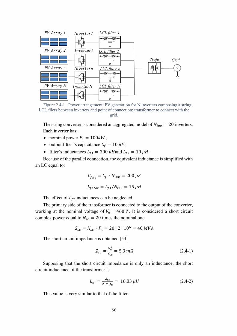
21 Motivation 45

22 Averaging versus switching models 45

23 Lumped model of a string 46

24 Current control 55

25 DC-link control 64

3 Frequency control with power electronic converter 67

31 Motivation 67

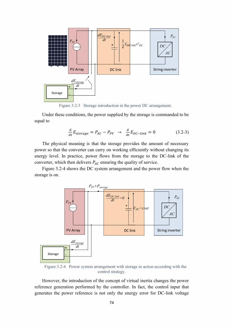
32 Power reference generation 71

33 Modification to the grid control 76

34 EnablingDisabling state of the storage 83

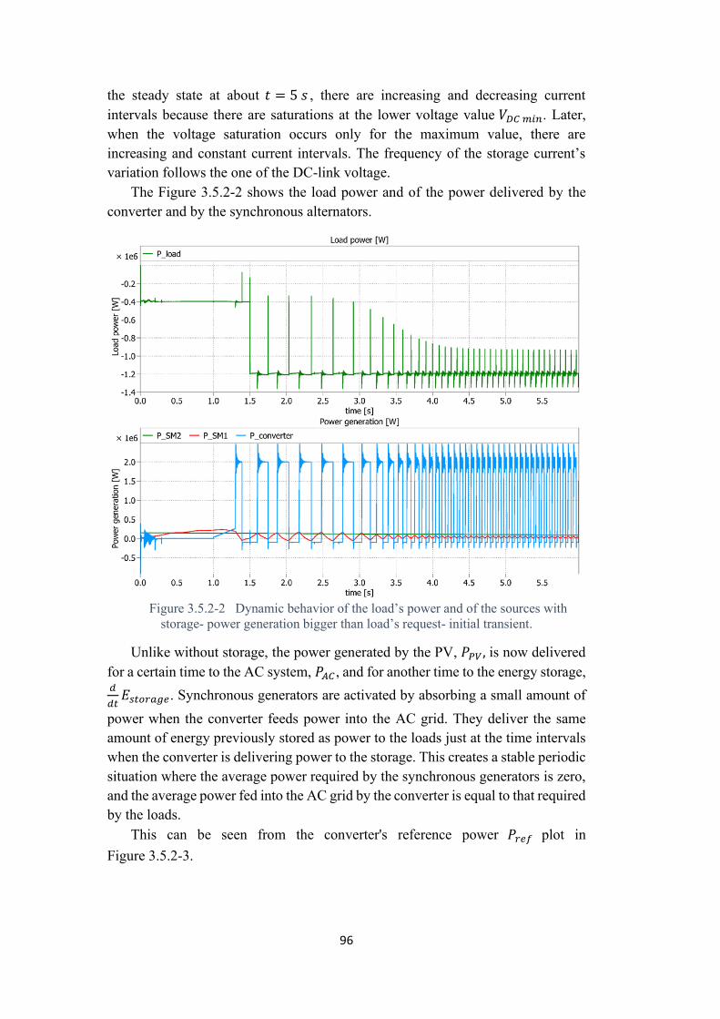
35 Case PVrsquos power generation bigger than loadrsquos request 91

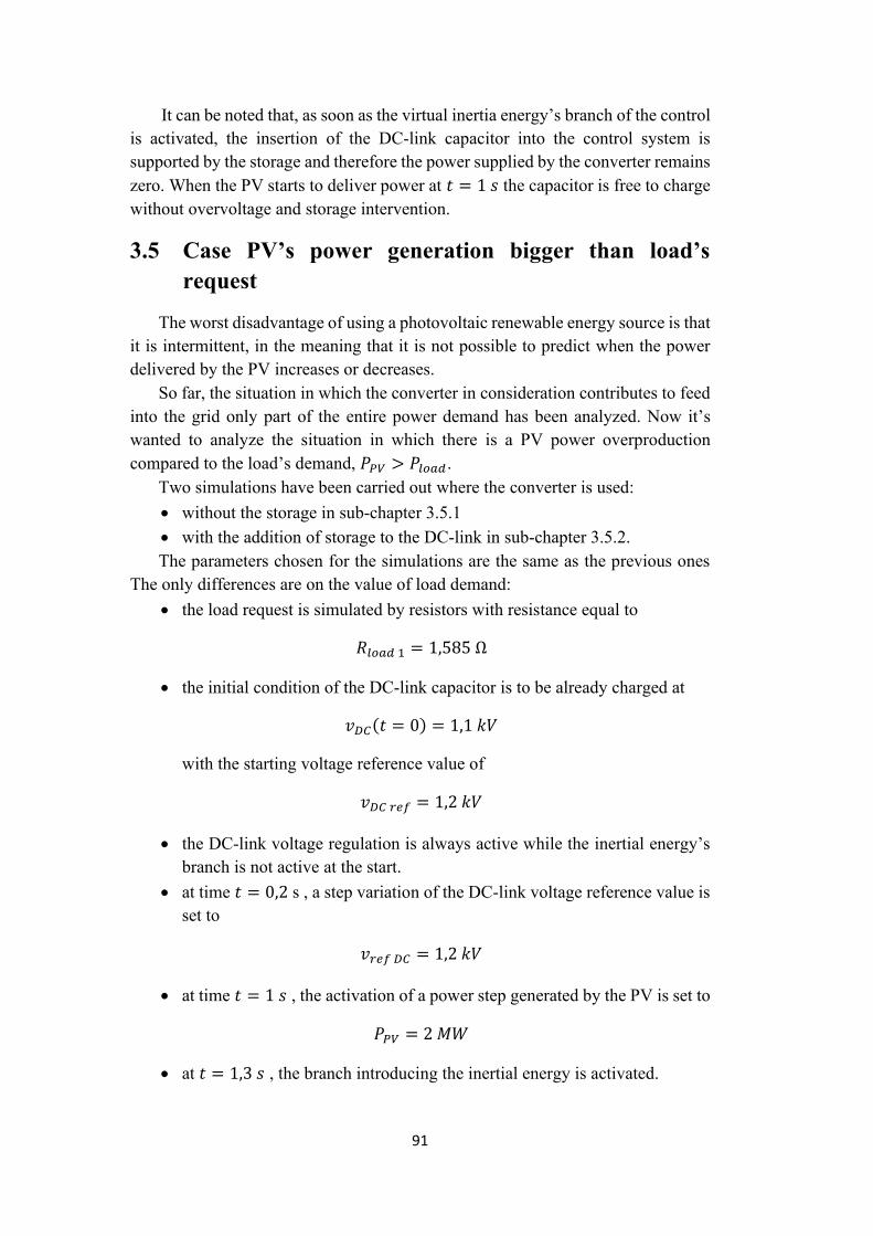
351 Without energy supplier 92

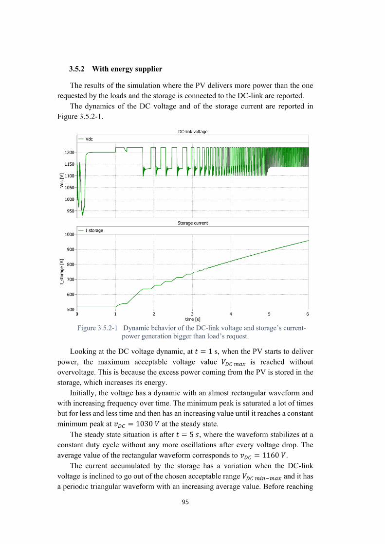
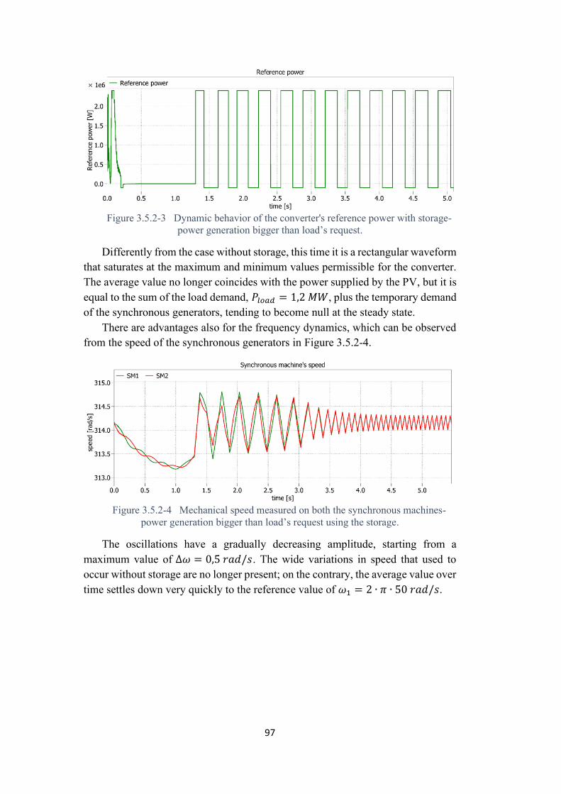
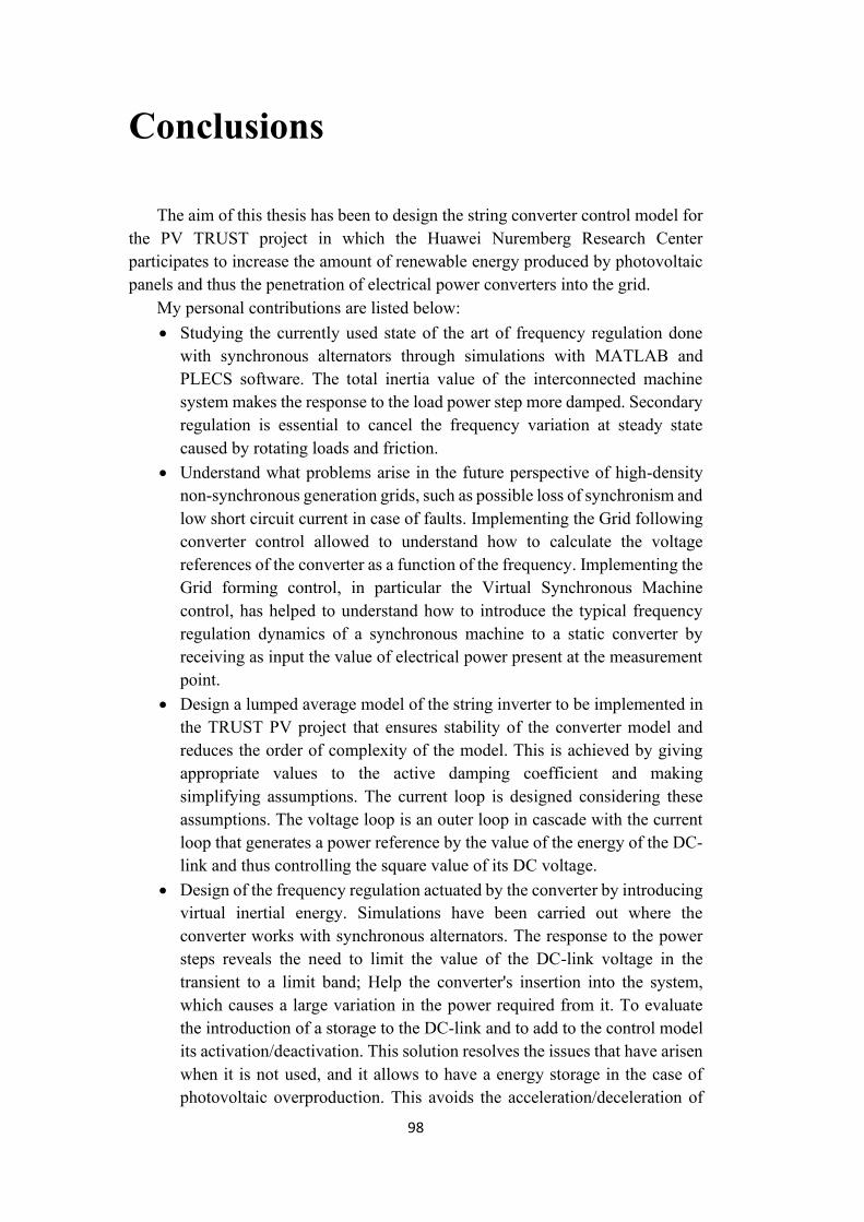
352 With energy supplier 95

Conclusions 98

List of Figures Figure 11-1 Steam turbinersquos schematic 4

Figure 11-2 Synchronous machine frequency regulation 5

Figure 11-3 Trends of frequency variation and power variation at the step loadrsquos power variation- References machine 7

Figure 11-1 SNPS trend in the years 2018 light purple 2019 dark purple and 2020 green in different places (a) NEM (b) New South Wales (c) Queensland (d) South Australia (e) Tasmania (f) Victoria [7] 20

Figure 12-2 Stator current of the synchronous machine during a short circuit event 21

Figure 12-3 Voltage and current of the converter during a short circuit event 22

Figure 12-4 PLL dynamic during a short circuit time interval of 005 s and 01 s 23

Figure 13-1 Grid following converter topology on the left and its phasors diagram on the right [21] 28

Figure 13-2 Grid following converter control block diagram 29

Figure 13-3 Grid following converter control principle droop control 29

Figure 13-4 Grid forming converter control block diagram 30

Figure 13-5 Grid forming converter control principle droop control 30

Figure 13-6 Grid forming converter topology on the left and its phasors diagram on the right [21] 30

Figure 13-7 Topology of the power electric circuit converter connected to the RLE grid trough RLC filter 31

Figure 111-1 Grid following converter control schematic

blockhelliphelliphelliphellip32

Figure 111-2 Grid following converter control active and reactive

power dynamics at a step reference variationhelliphelliphelliphelliphelliphelliphelliphelliphelliphelliphelliphelliphelliphelliphelliphellip34

Figure 111-3 Grid following converter control dq-axis current

dynamic at a step reference variationhelliphelliphelliphelliphelliphelliphelliphelliphelliphelliphelliphelliphelliphelliphelliphelliphelliphelliphelliphellip35

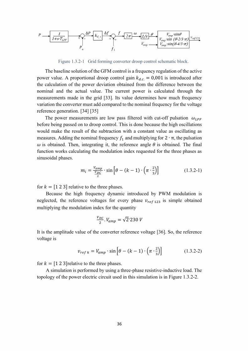
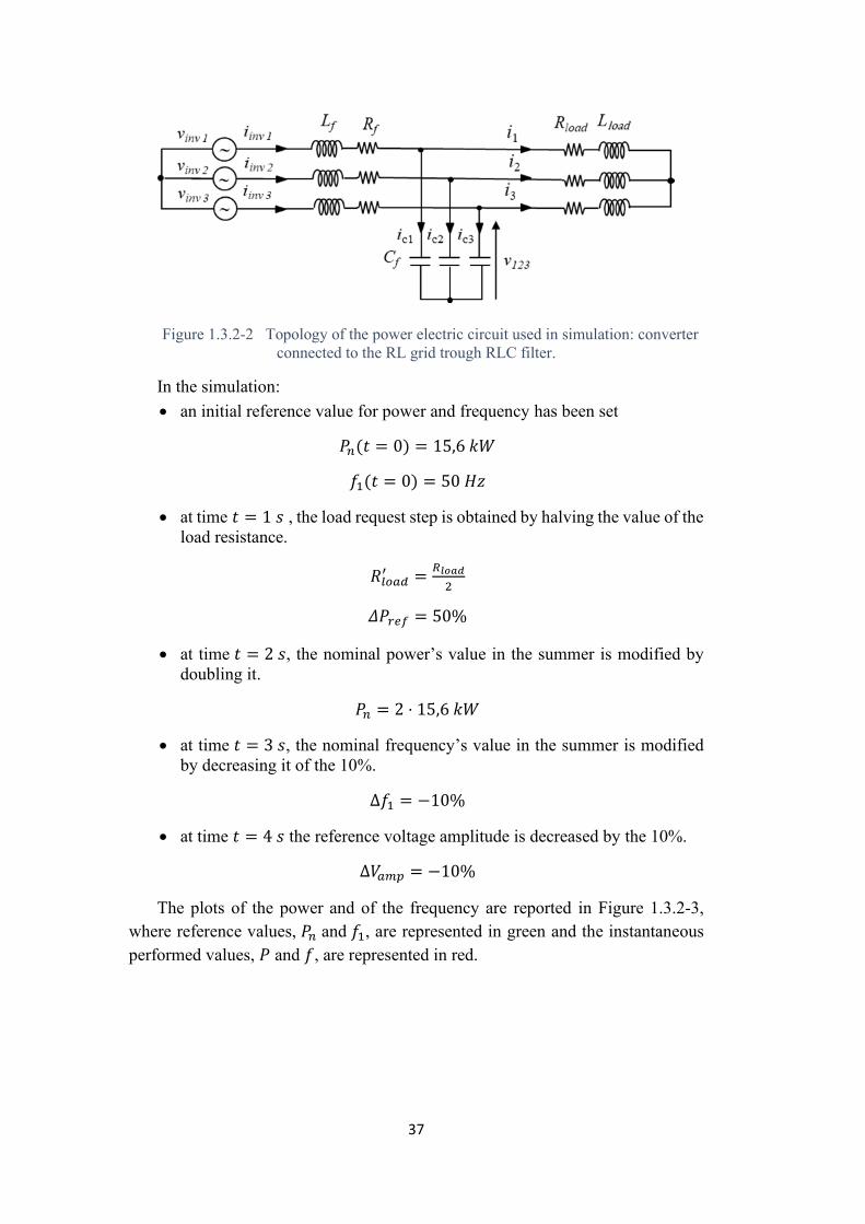
Figure 132-1 Grid forming converter droop control schematic blockhellip 36 Figure 112-2 Topology of the power electric circuit used in simulation

converter connected to the RL grid trough RLC filterhelliphelliphelliphelliphelliphelliphelliphelliphelliphelliphelliphellip37

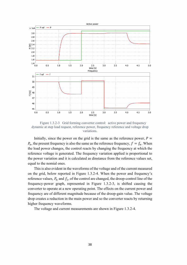
Figure 112-3 Grid forming converter control active power and

frequency dynamic at step load request reference power frequency

reference and voltage drop variationshelliphelliphelliphelliphelliphelliphelliphelliphelliphelliphelliphelliphelliphelliphelliphelliphelliphelliphelliphelliphellip38

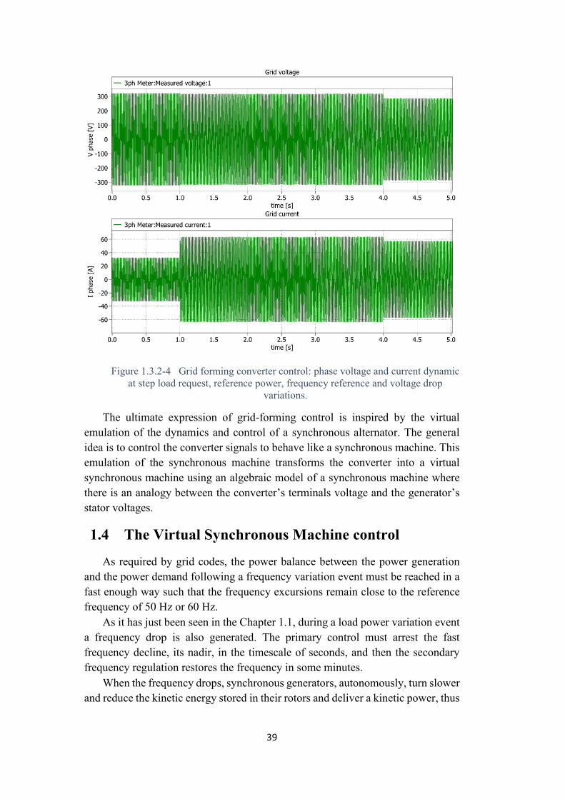
Figure 112-4 Grid forming converter control phase voltage and

current dynamic at step load request reference power frequency reference

and voltage drop variationshelliphelliphelliphelliphelliphelliphelliphelliphelliphelliphelliphelliphelliphelliphelliphelliphelliphelliphelliphelliphelliphelliphelliphelliphelliphellip39

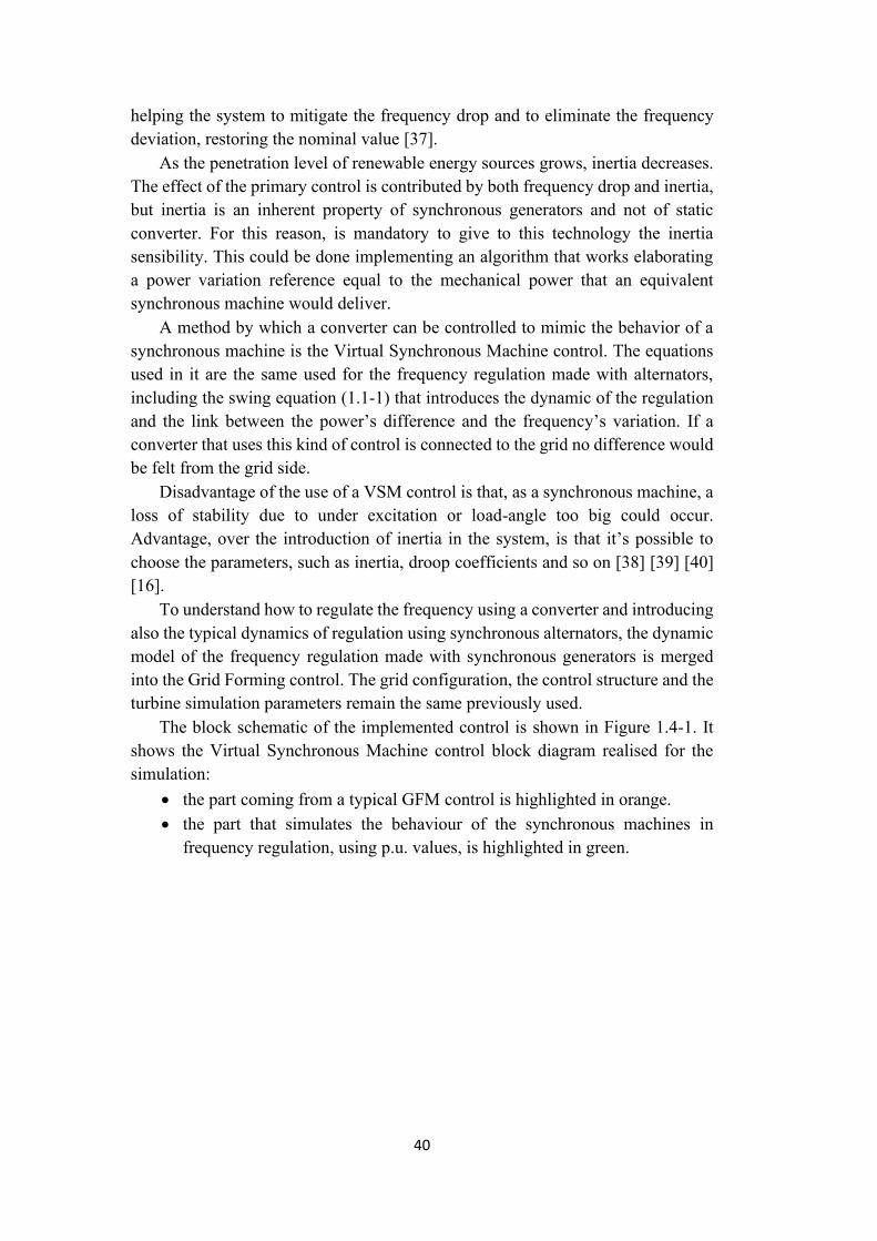
Figure 14-1 Grid forming converter Virtual Synchronous Machine control schematic block in orange the part coming from a typical GFM control in green the part that simulates the synchronous machine frequency regulations behavior 41

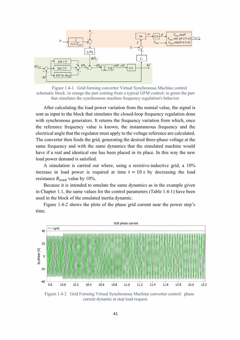
Figure 14-2 Grid Forming Virtual Synchronous Machine converter control phase current dynamic at step load request 41

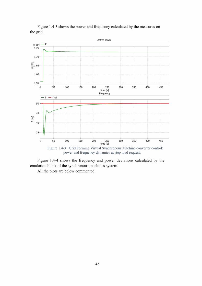
Figure 14-3 Grid Forming Virtual Synchronous Machine converter control power and frequency dynamics at step load request 42

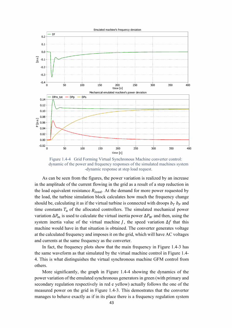
Figure 14-4 Grid Forming Virtual Synchronous Machine converter control dynamic of the power and frequency responses of the simulated machines system -dynamic response at step load request 43

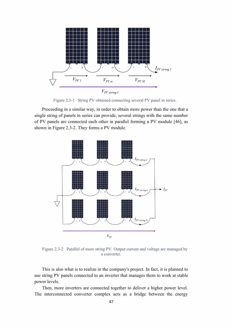
Figure 23-1 String PV obtained connecting several PV panel in series 47

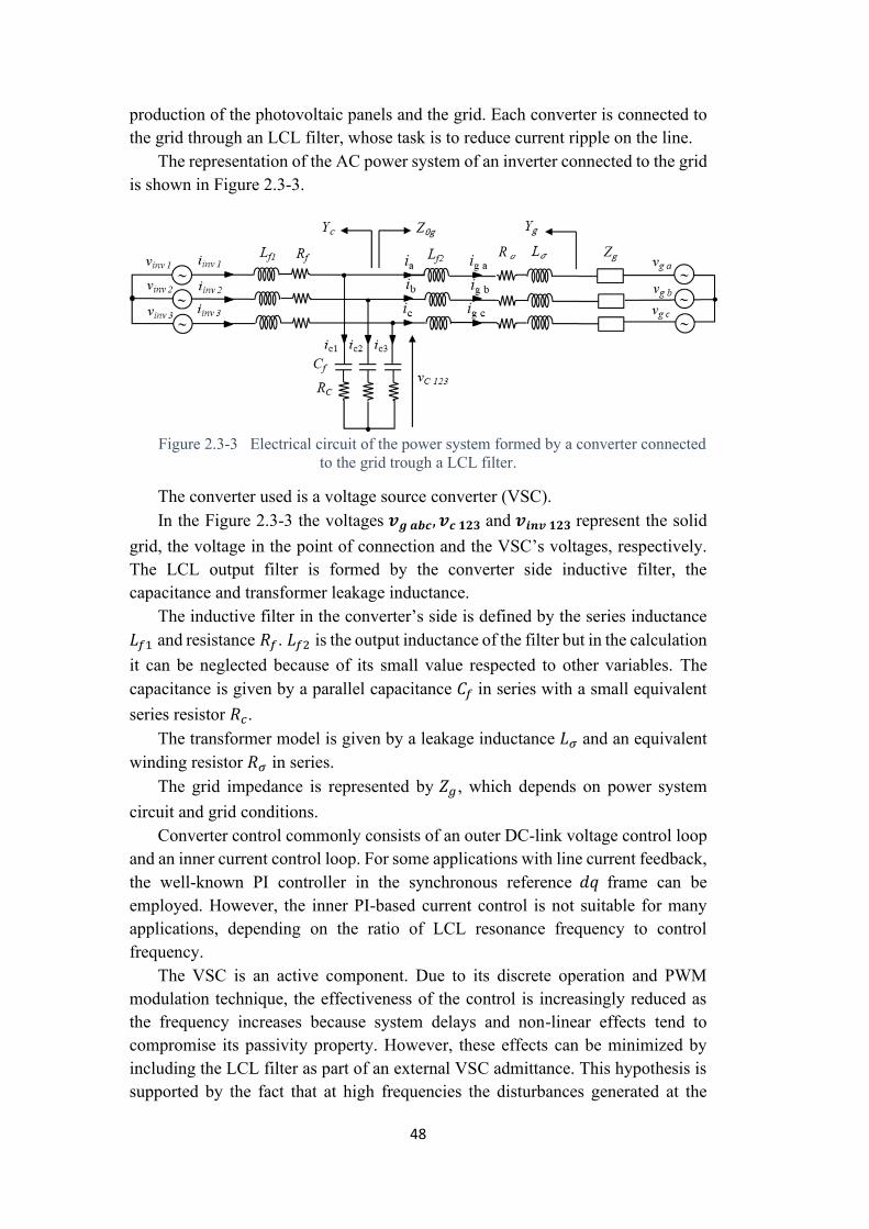
Figure 23-2 Parallel of more string PV Output current and voltage are managed by a converter 47

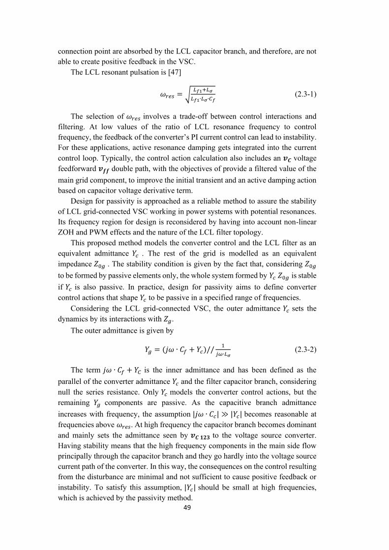
Figure 23-3 Electrical circuit of the power system formed by a converter connected to the grid trough a LCL filter 48

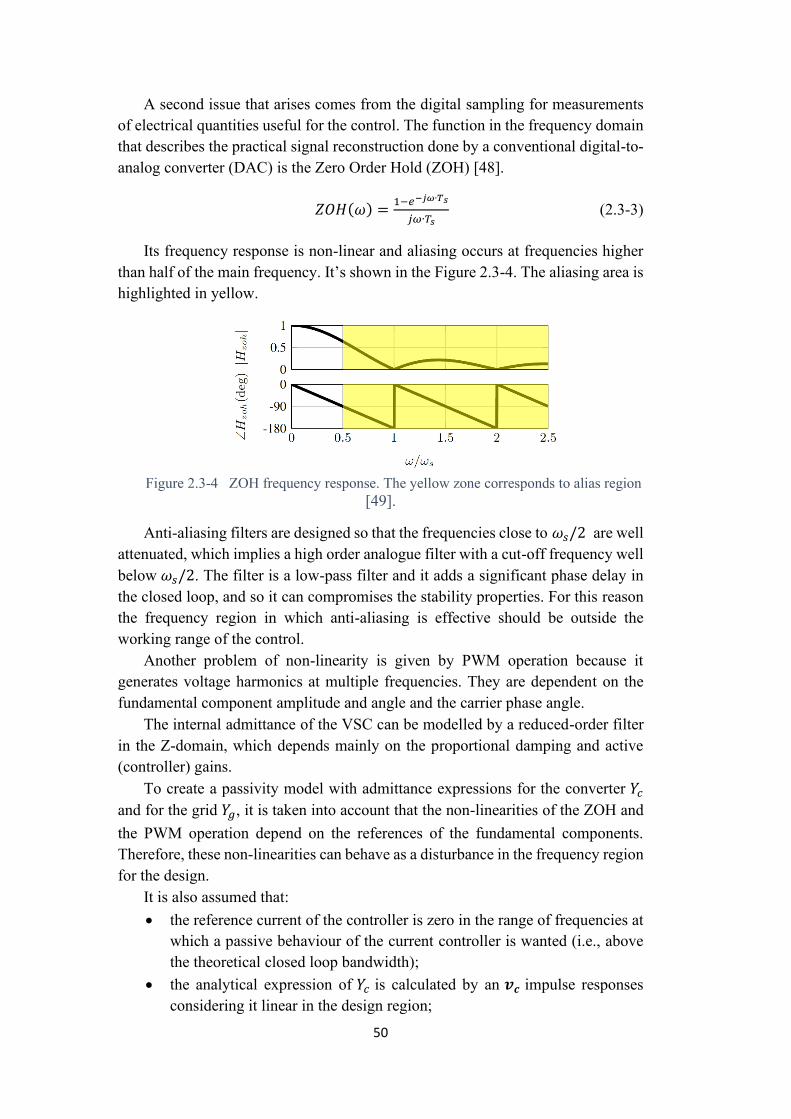
Figure 23-4 ZOH frequency response The yellow zone corresponds to alias region [49] 50

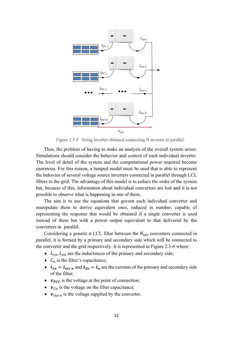
Figure 23-5 String inverter obtained connecting N inverter in parallel 52

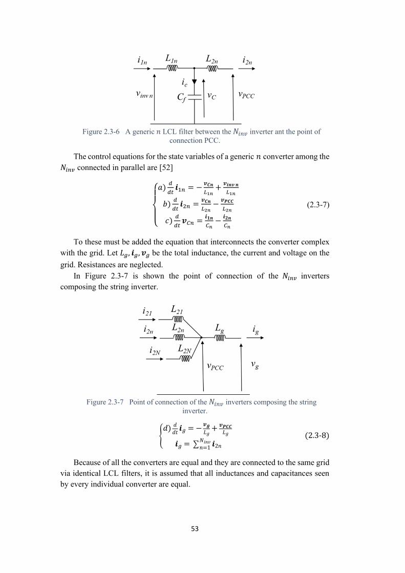
Figure 11-6 A generic n LCL filter between the Ninv inverter ant the point of connection PCChelliphelliphelliphelliphelliphelliphelliphelliphelliphelliphelliphelliphelliphelliphelliphelliphelliphelliphelliphelliphelliphelliphelliphelliphelliphelliphelliphelliphelliphelliphellip53

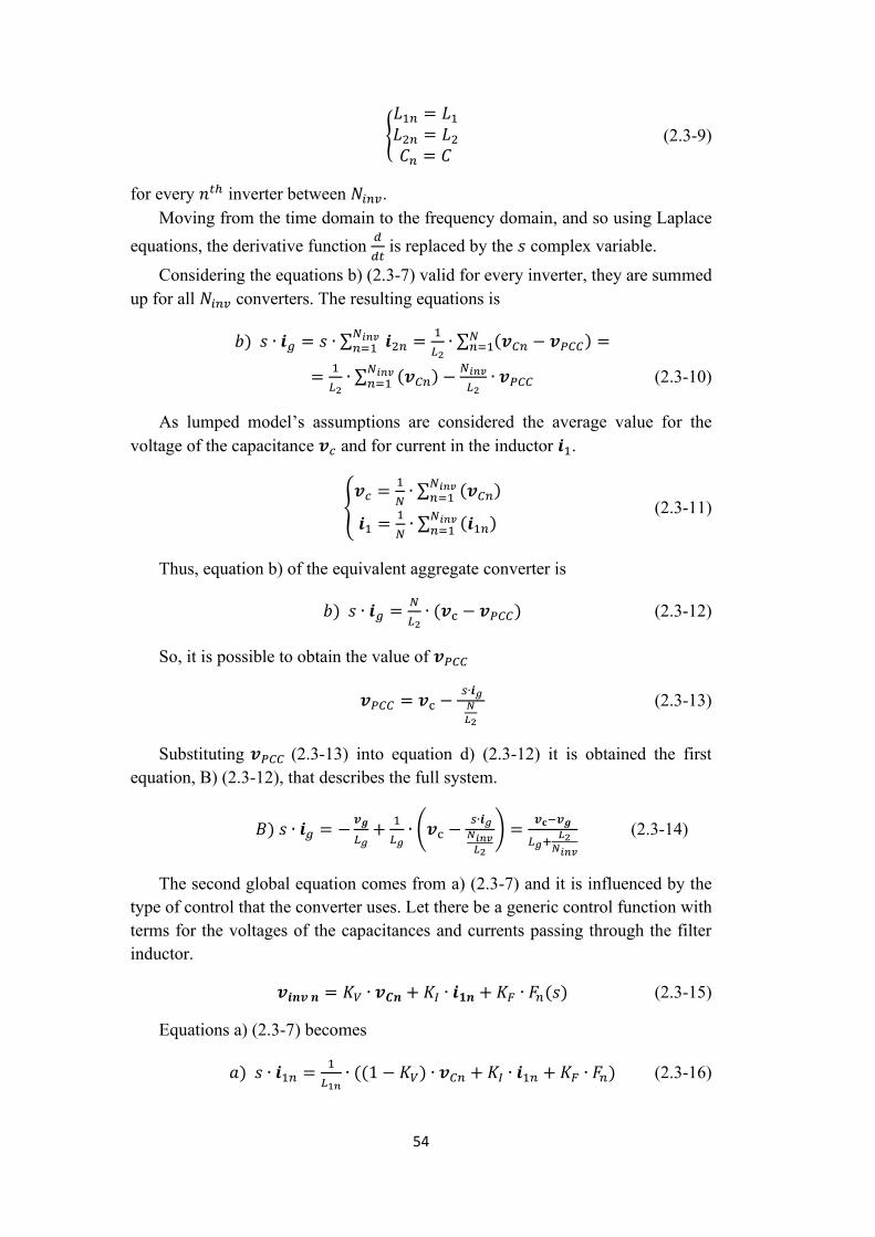
Figure 11-7 Point of connection of the Ninv inverters composing the

string inverterhelliphelliphelliphelliphelliphelliphelliphelliphelliphelliphelliphelliphelliphelliphelliphelliphelliphelliphelliphelliphelliphelliphelliphelliphelliphelliphelliphelliphelliphelliphelliphelliphelliphellip54

Figure 24-1 Power arrangement PV generation for N inverters composing a string LCL filers between inverters and point of connection transformer to connect with the grid 56

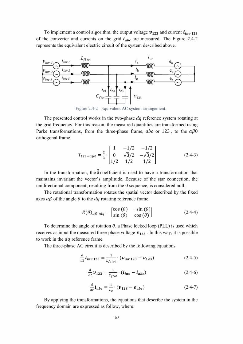
Figure 24-2 Equivalent AC system arrangement 57

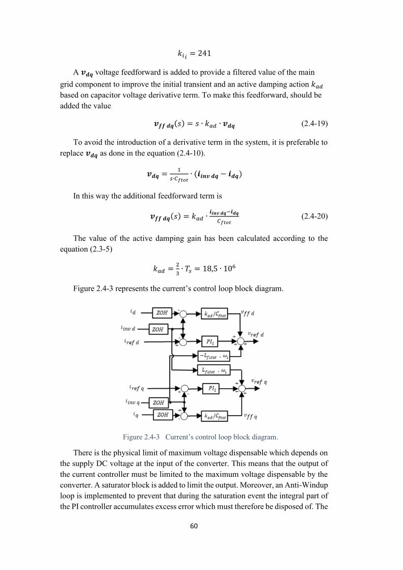
Figure 24-3 Currentrsquos control loop block diagram 60

Figure 24-4 Currentrsquos control loop block diagram with saturators and anti-windup 62

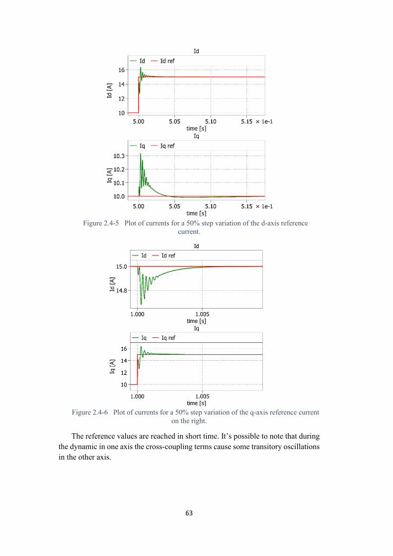
Figure 24-5 Plot of currents for a 50 step variation of the d-axis reference current 63

Figure 24-6 Plot of currents for a 50 step variation of the q-axis reference current on the right 63

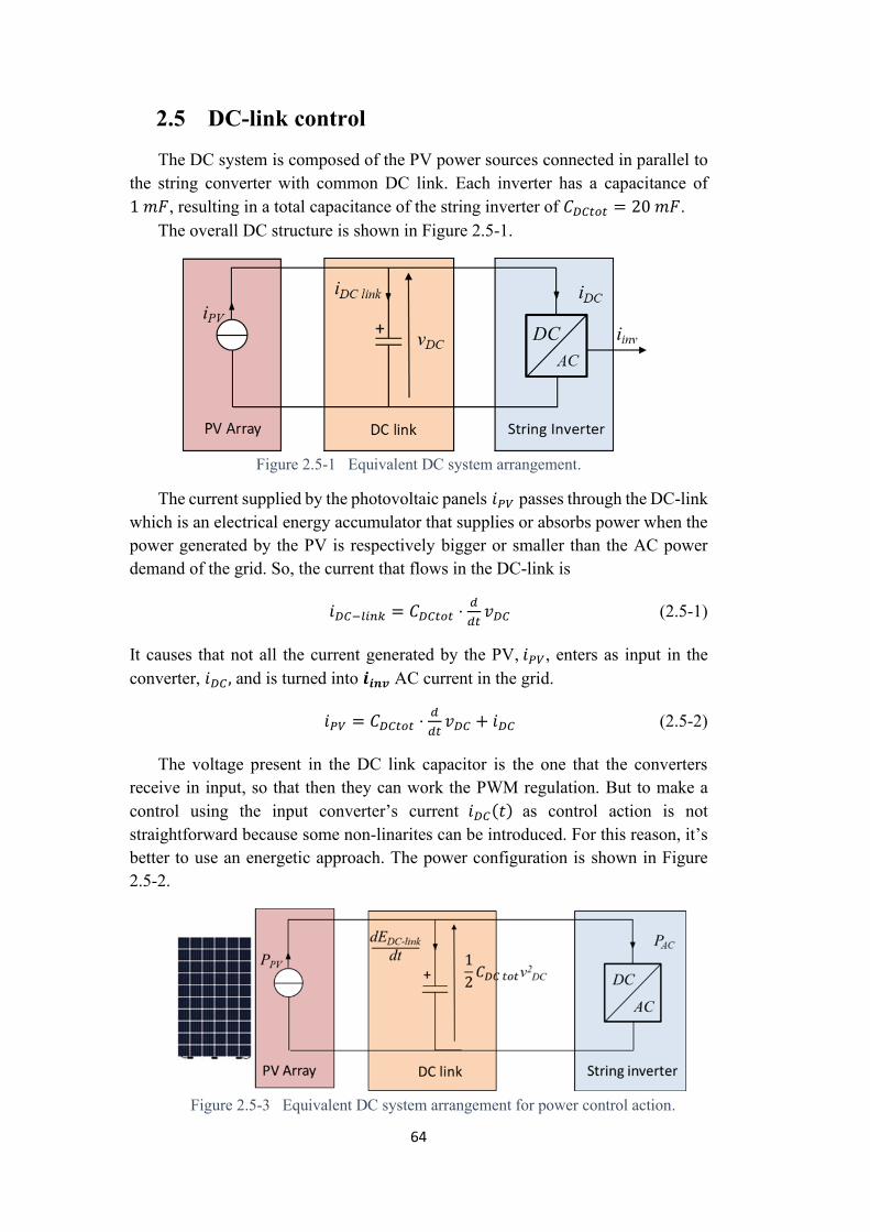
Figure 25-1 Equivalent DC system arrangement 64

Figure 25-2 Equivalent DC system arrangement for power control action 64

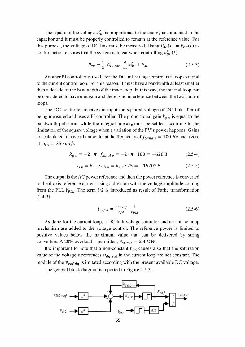
Figure 25-3 DC-link voltagersquos control loop block diagram 66

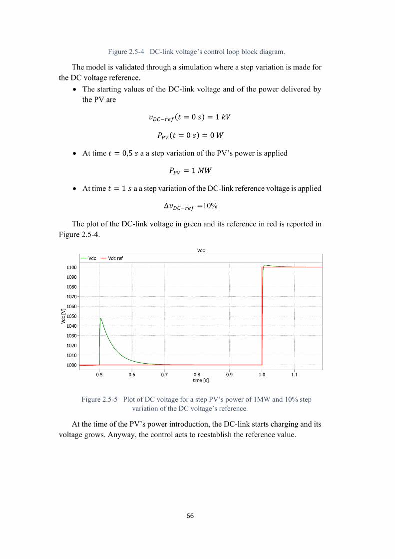
Figure 25-4 Plot of DC voltage for a step PVrsquos power of 1MW and 10 step

variation of the DC voltagersquos reference 66

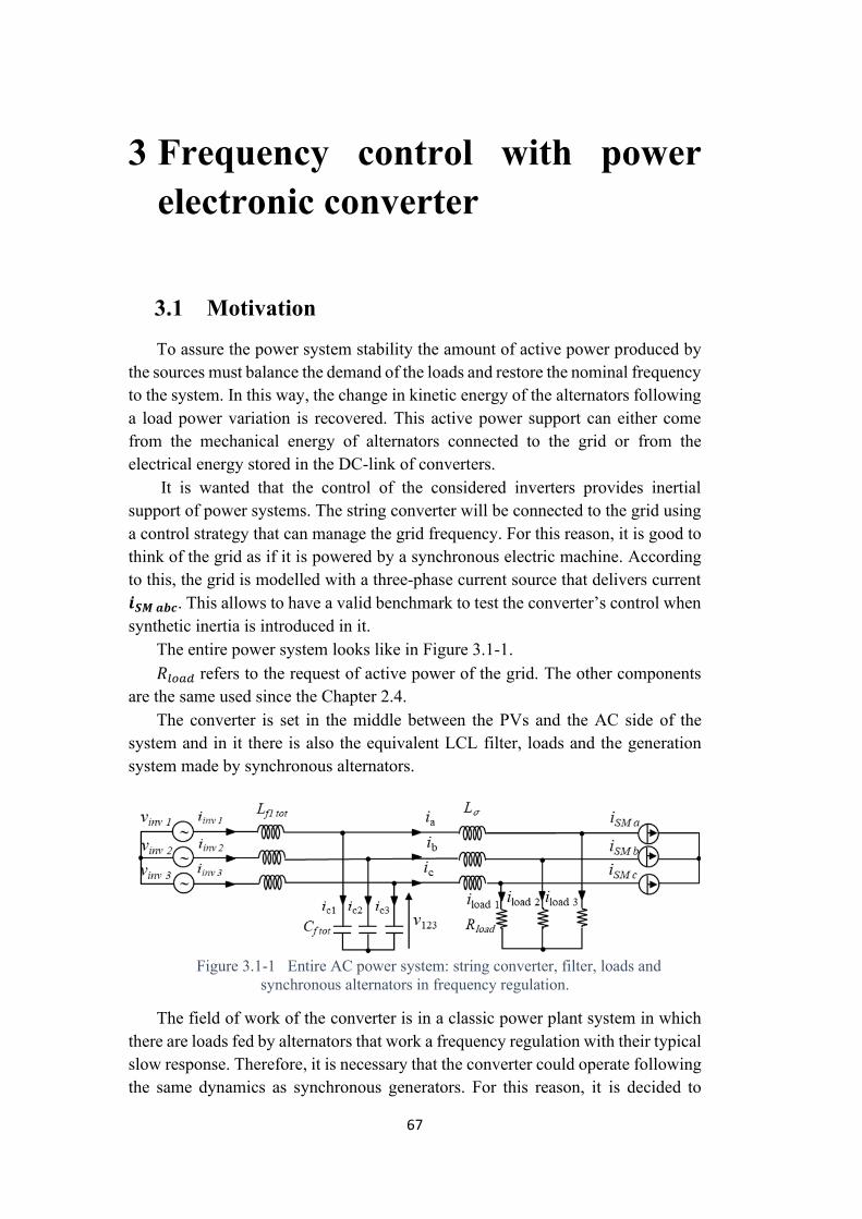
Figure 31-1 Entire AC power system string converter filter loads and synchronous alternators in frequency regulation 67

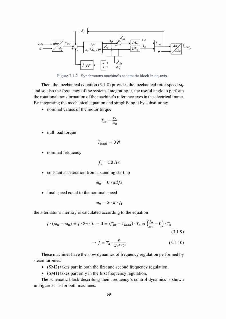
Figure 31-2 Synchronous machinersquos schematic block in dq-axis 69

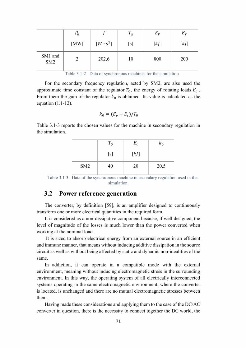
Figure 32-1 DC-link voltage and energy calculation schematic block and energetic inputs for the DC voltage control 72

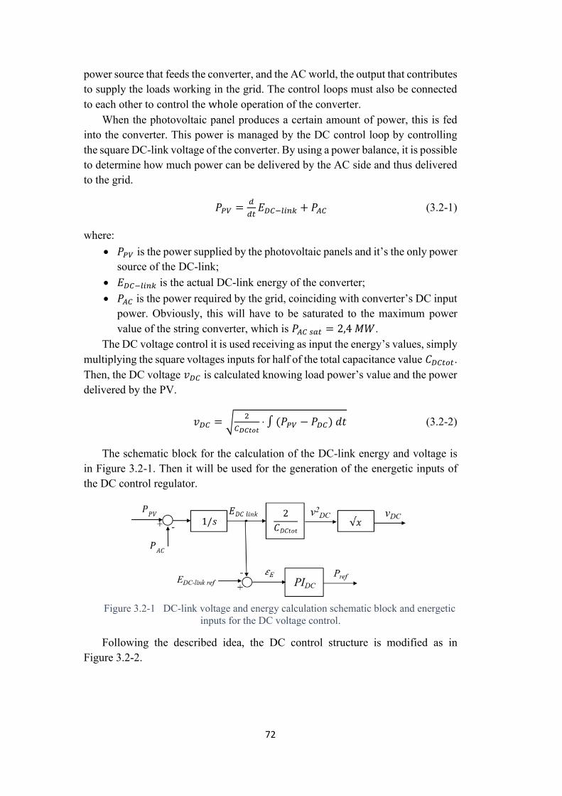
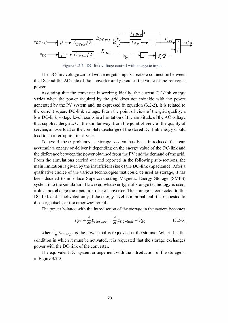
Figure 32-2 DC-link voltage control with energetic inputs 73

Figure 32-3 Storage introduction in the power DC arrangement 74

Figure 32-4 Power system arrangement with storage in action according with the control strategy 74

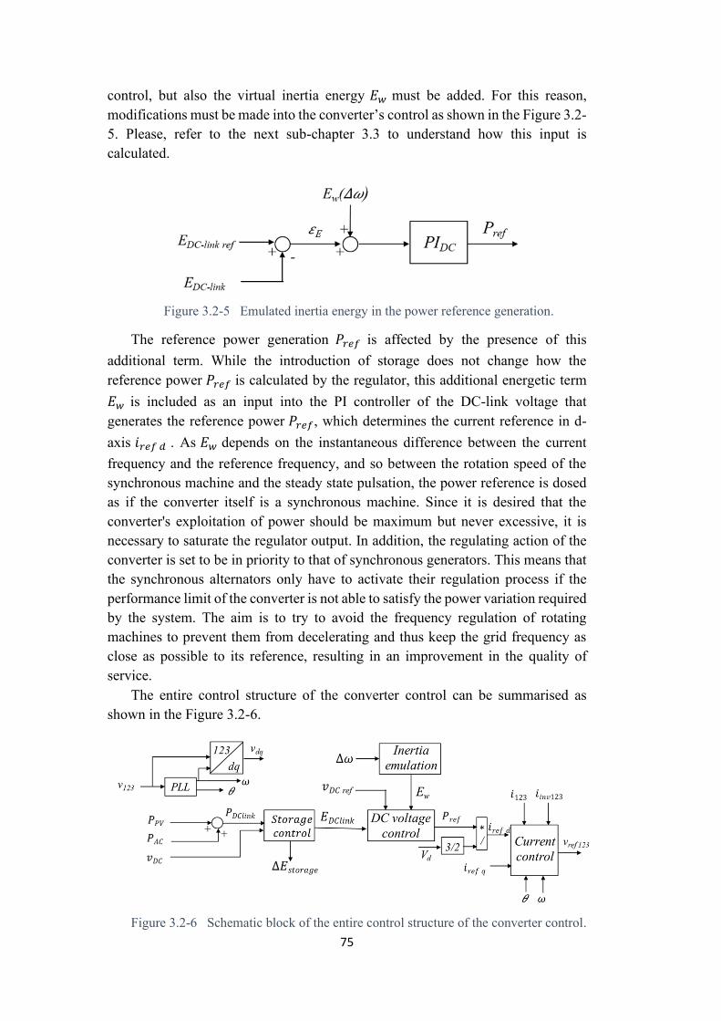
Figure 32-5 Emulated inertia energy in the power reference generation 75

Figure 32-6 Schematic block of the entire control structure of the converter control 75

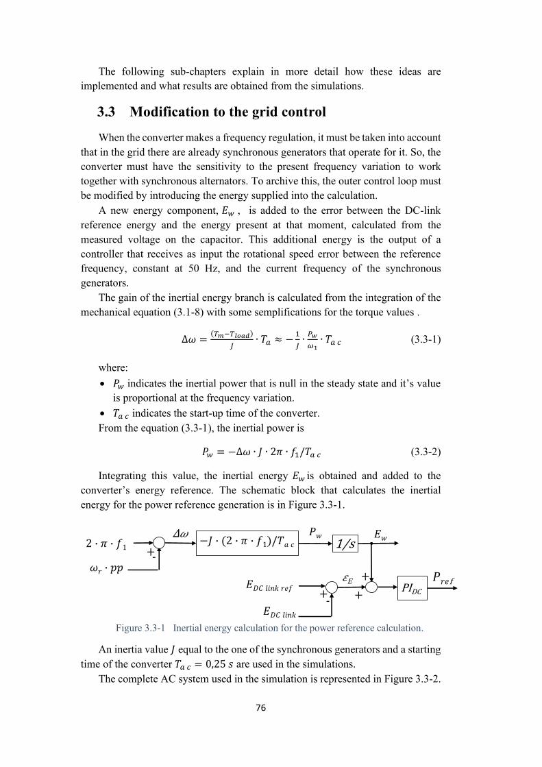
Figure 33-1 Inertial energy calculation for the power reference calculation 76

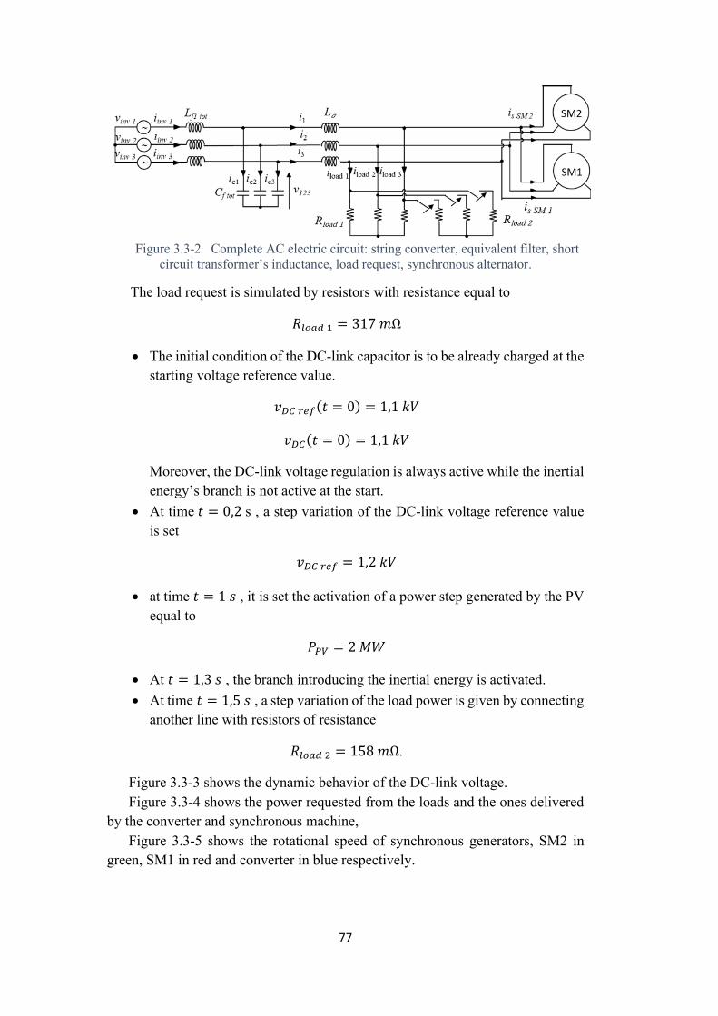
Figure 33-2 Complete AC electric circuit string converter equivalent filter short circuit transformerrsquos inductance load request synchronous alternator 77

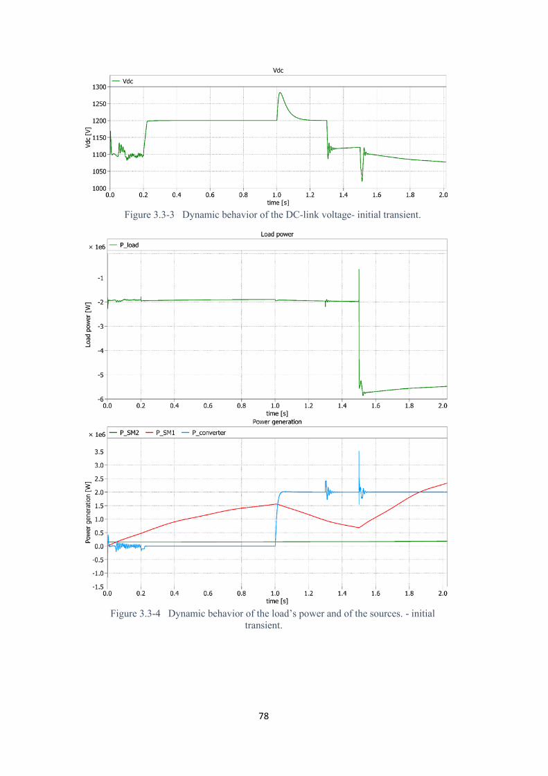
Figure 33-3 Dynamic behavior of the DC-link voltage- initial transient 78

Figure 33-4 Dynamic behavior of the loadrsquos power and of the sources - initial transient 78

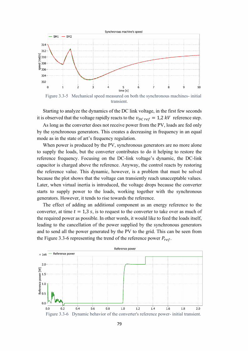
Figure 33-5 Mechanical speed measured on both the synchronous machines- initial transient 79

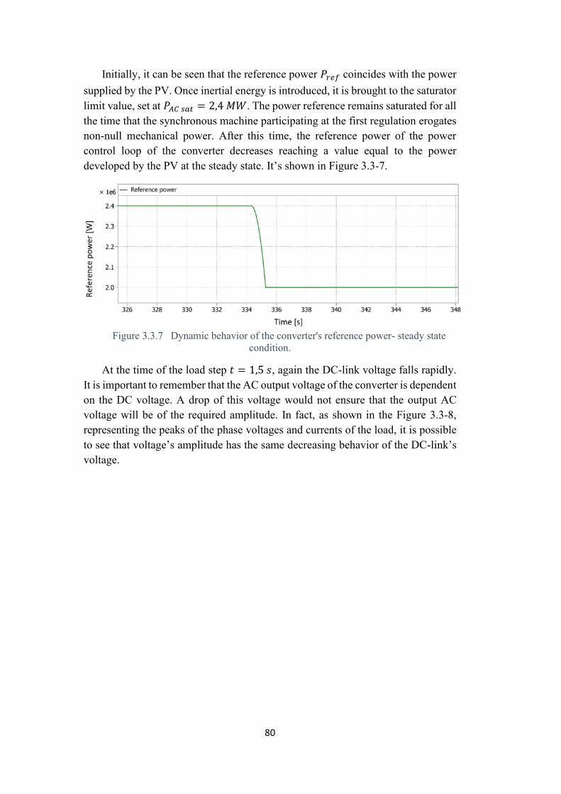
Figure 33-6 Dynamic behavior of the converters reference power- initial transient 79

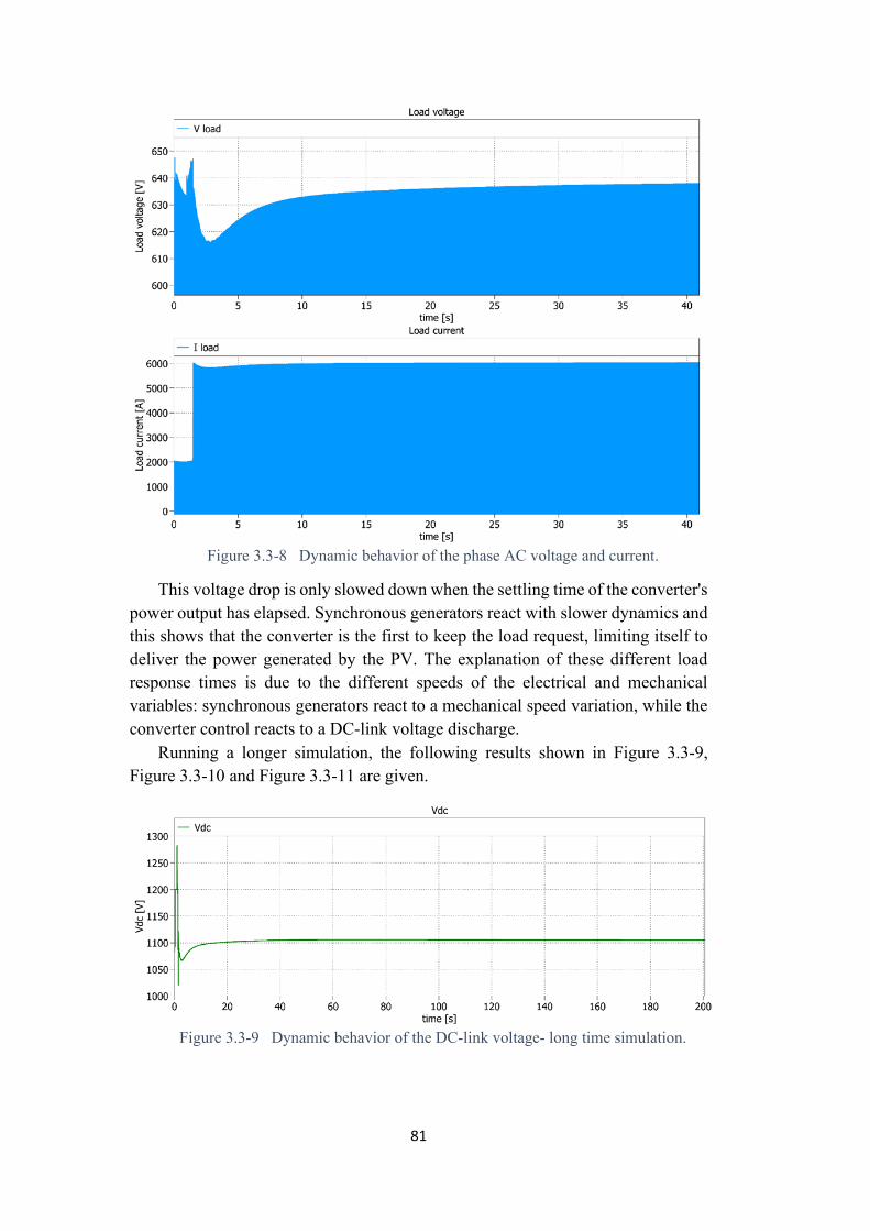
Figure 33-7 Dynamic behavior of the phase AC voltage and current 81

Figure 33-8 Dynamic behavior of the DC-link voltage- long time simulation 81

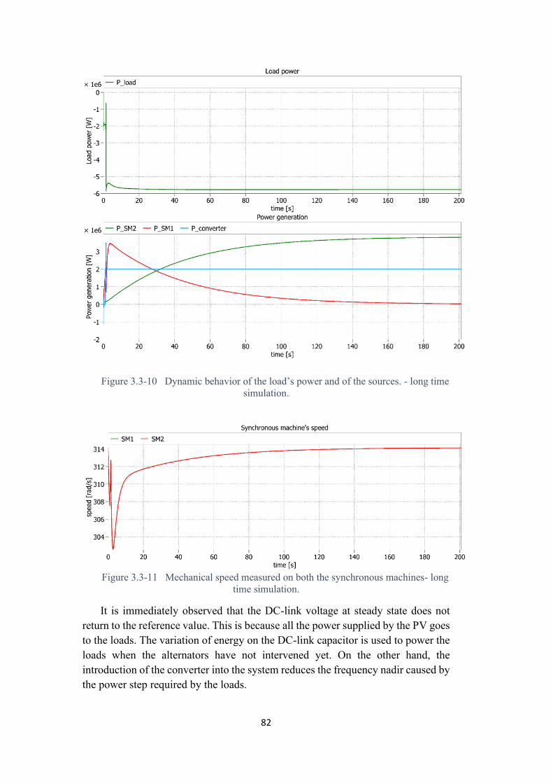
Figure 33-9 Dynamic behavior of the loadrsquos power and of the sources - long time simulation 82

Figure 33-10 Mechanical speed measured on both the synchronous machines- long time simulation 82

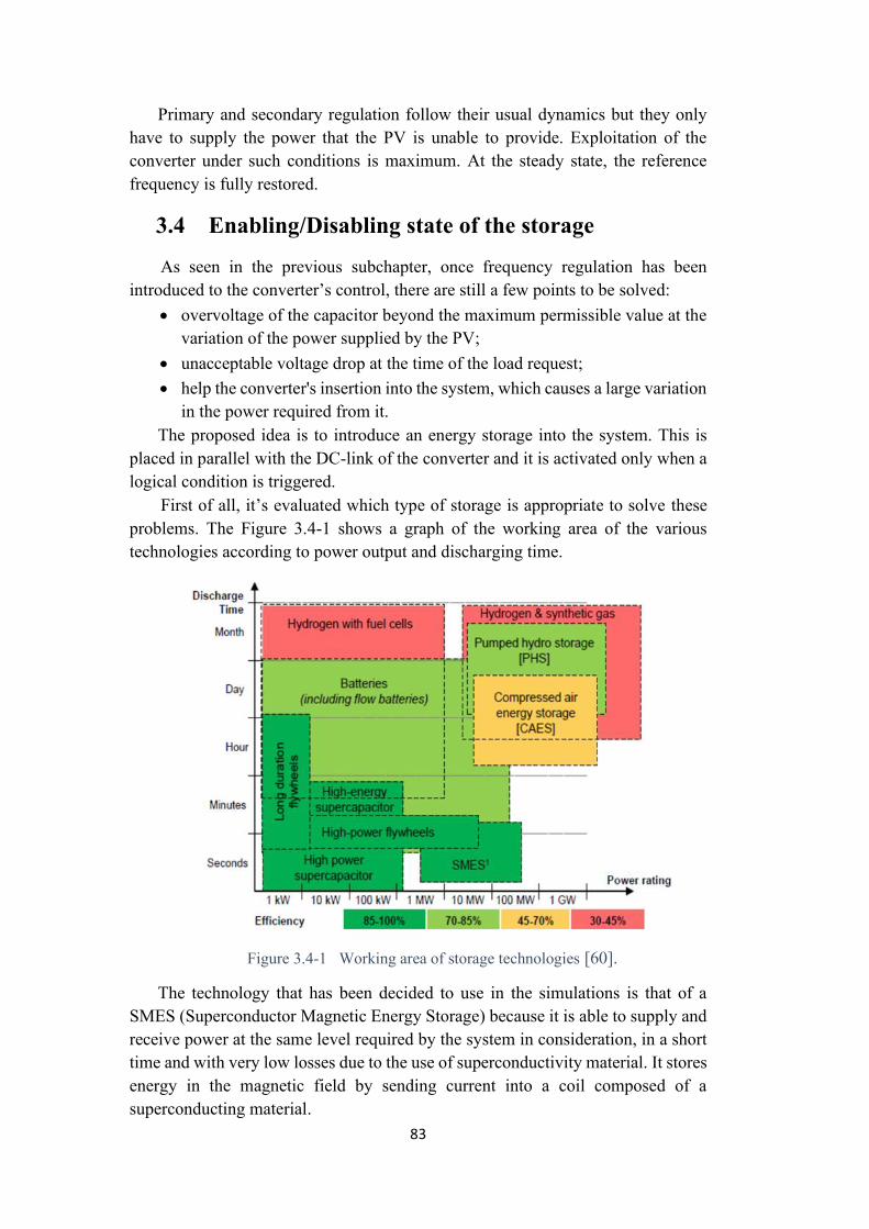
Figure 34-1 Working area of storage technologies [60] 83

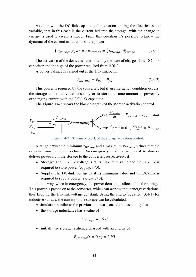
Figure 34-2 Schematic block of the storage activation control 84

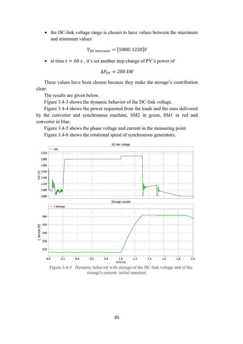
Figure 34-3 Dynamic behavior with storage of the DC-link voltage and of the storages current- initial transient 85

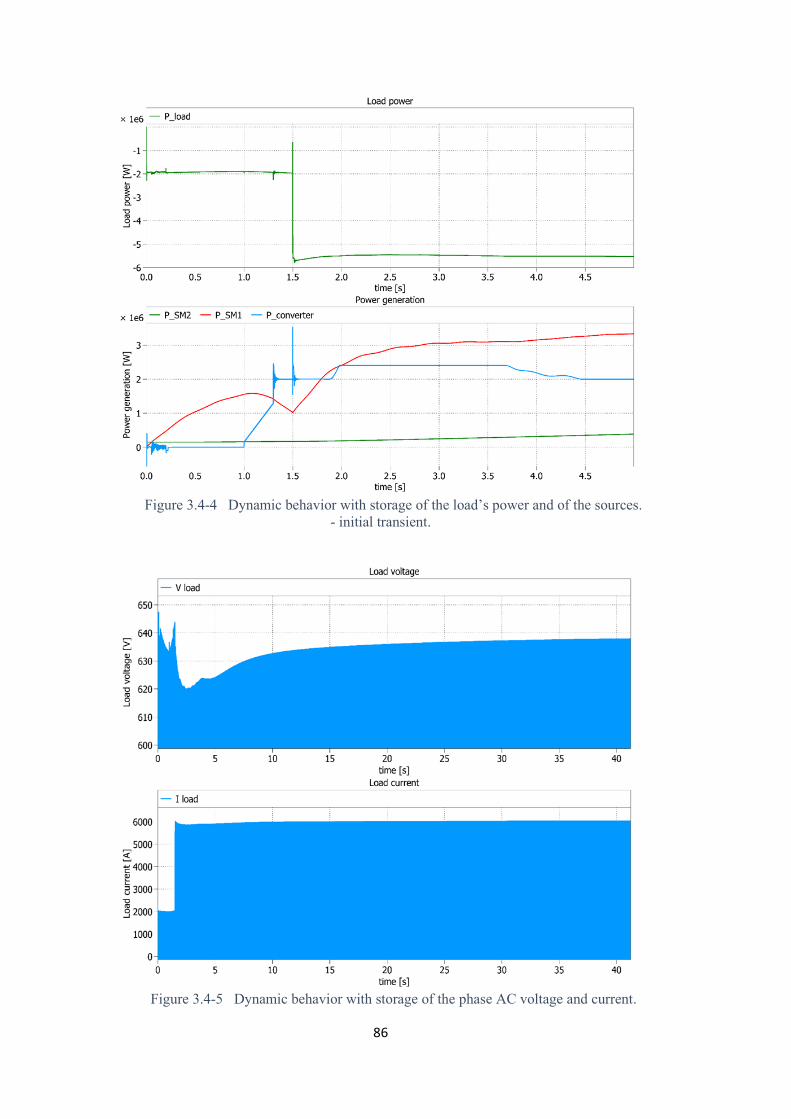
Figure 34-4 Dynamic behavior with storage of the loadrsquos power and of the

sources - initial transient 86

Figure 34-5 Dynamic behavior with storage of the phase AC voltage and current 86

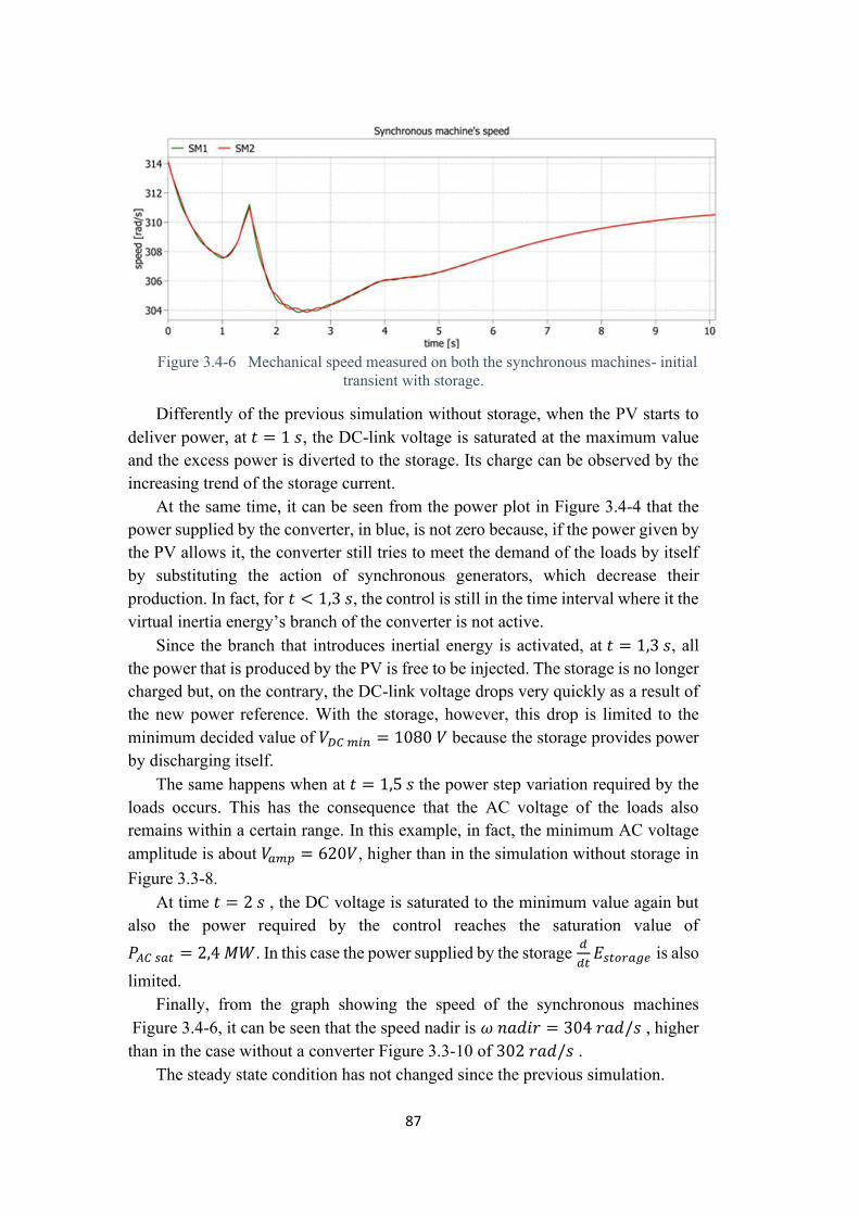
Figure 34-6 Mechanical speed measured on both the synchronous machines- initial transient with storage 87

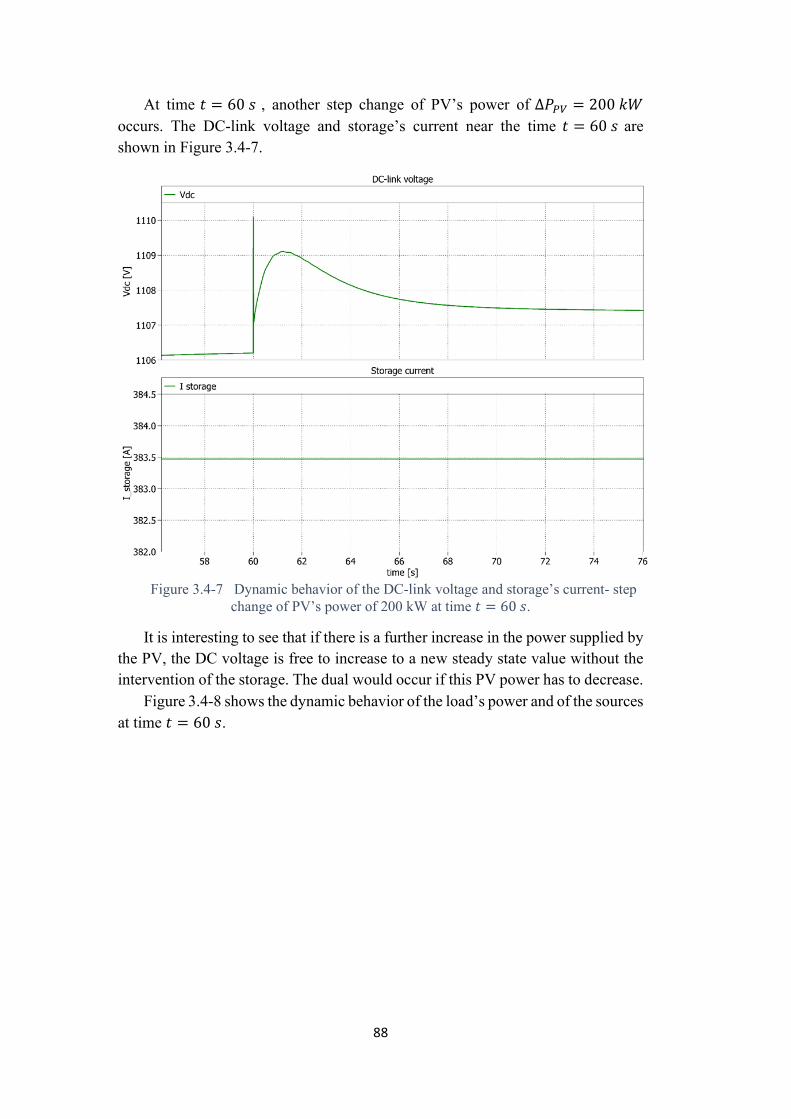
Figure 34-7 Dynamic behavior of the DC-link voltage and storagersquos

current- step change of PVrsquos power of 200 kW at time t=60 shelliphelliphelliphelliphellip91

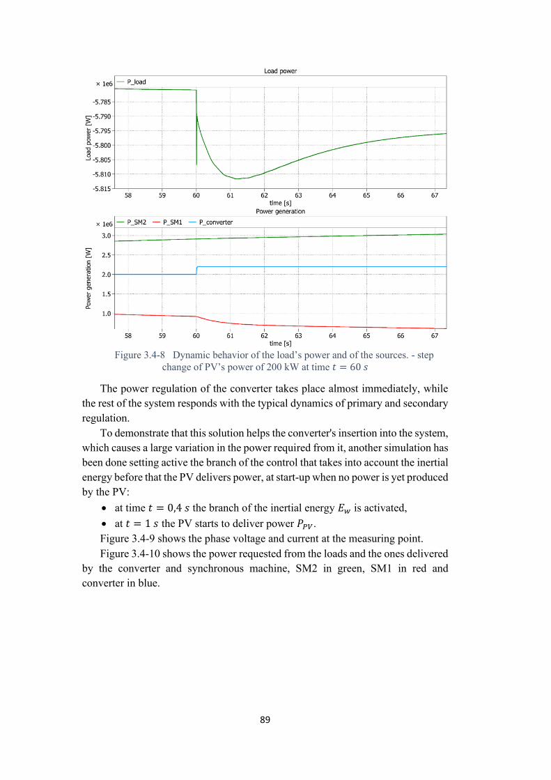
Figure 34-8 Dynamic behavior of the loadrsquos power and of the sources - inertial energy is activated at time 119905 = 04 119904- initial transient 90

Figure 351-1 Dynamic behavior of the DC-link voltage- power generation bigger than loadrsquos request 92

Figure 351-2 Dynamic behavior of the loadrsquos power and of the sources - power generation bigger than loadrsquos request 93

Figure 351-3 Mechanical speed measured on both the synchronous machines- power generation bigger than loadrsquos request 93

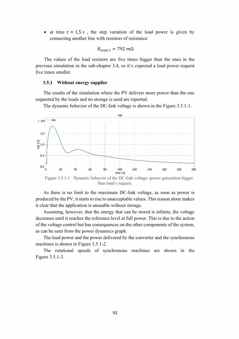
Figure 351-4 Dynamic behavior of the converters reference power- power generation bigger than loadrsquos request 94

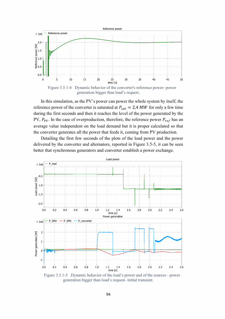
Figure 351-5 Dynamic behavior of the loadrsquos power and of the sources - power generation bigger than loadrsquos request- initial transient 94

List of Tables Table 11-1 Data of the references synchronous machine 6

Table 11-2 Dynamic results at the step loadrsquos power variation - One synchronous machine in first frequency regulation 8

Table 11-3 Open loop poles closed loop poles and damping for various synchronous machine in first frequency regulation 10

Table 11-4 Data of the two different machines in first frequency regulation end of the one non participant 11

Table 11-5 Dynamic results at the step loadrsquos power variation- Two different synchronous machines in first frequency regulation and one non participant 13

Table 11-6 Data of the machines in first frequency regulation in secondary frequency regulation and one non participant 15

Table 12-1 Short-term solutions and long-term solutions for low inertia systems 26

Table 31 1 Data of the droops and time constants of the synchronous machines used in the simulationhelliphelliphelliphelliphelliphelliphelliphelliphelliphelliphelliphelliphelliphelliphelliphelliphelliphelliphelliphelliphelliphelliphellip69

Table 31-2 Data of synchronous machines for the simulation 71

Table 31-3 Data of the synchronous machine in secondary regulation used in the simulation 71

List of Acronyms and Symbols

Symbol Meaning 119864119889119890119888 Deceleration energy during fault

119864119875 Regulated permenten energy 119864119879 Regulated transient energy

119864119886119888119888 Accumulated energy during fault 119864119888 Energy of rotating loads

119864119890119888119888 Eccitationrsquos voltage 119864119908 Inertial energy 119866119891 Transfer function of the regulator

119867119874119871 Open loop transfer function 119875119871 Loadrsquos power request 119875119875 Power delivered by SM in first frequency regulation

119875119886119904 Asynchronous power of the machinersquos damping

windings 119875119888 Power of rotating loads 119875119890 Electrical power 119875119898 Mechanical power 119875119904 Power delivered by SM in secondary frequency

regulation 119875119908 Inertial power

119877(120579)120572120573rarr119889119902 Rotational transformation 119877119905ℎ Boilerrsquos thermal resistance 1198790 Secondary fraquency regulation time constant

119879123rarr120572120573 Parke transformations 119879119886 119888 Start-up time of the converter 119879119886 Start up time 119879119901 Pole time constant 119879119904 Sampling period 119879119911 Zero time constant

119881119886119898119901 Amplitude value of the converter reference voltage 119884119888 Equivalent admittance of converter and filter 119884119892 Equivalent admittance of converter filter and

transformer 1198850119892 Equivalent impedance of grid and transformer 119887119875 Permanent droop 119887119879 Transitory droop

119889

119889119905 Time derivate

119891119904 Sampling frequency 119896 119901 Proportional gain of the regulator 1198960 Secondary fraquency regulation gain

119896119886119889 Active damping gain 119896119889 Direct feedthrough gain of anti-windup

119896119889119888 Droop control gain 119896119891119889119887 Feedback gain of anti-windup 119896119894 Integral gain of the regulator

119898 Modulation index 119901plusmn Poles

119901119888119900119899119907 Converterrsquos pole 120596119888 Crossover pulsation

120596119899119886119905 Natural pulsation ^T Transposed _0 Initial value

_1 Fundamental value _abc _123 Three-phase

_b Base value _band Bandwidth

_C Value on filter capacitance _cr Critical value _dq Two-phase rotating frame of reference d-axisrsquos

direction equal to voltage phase _f Value of filter component _ff Feedforward _g Gridrsquos value _i Relative to the current control loop

_inv Value on converter output _load Loadrsquos value _LPF Low pass filter _max Maximum value _min Minimum value

_n Nominal value _r Rotor

_ref Reference value _res Value of resonance _s Stator

_sat Saturation limit _sc Short circuit value _tot Equivalent total value _v Relative to the voltage control loop _σ Leakage value due to the transformer

cosϕ Power factor DAC Digital-to-analog converter F _F Control function of the converter GFL Grid following converter GFM Grid forming converter

ℎ Henthalpy variation HP High pressur step of the steam turbine J System inertia constant LP Low pressur step of the steam turbine

PCC Point of connection PI Proportional integaral controller

PLL Phase locked loop PV Photovoltaic

PWM Pulse width modulation qf Quality factor

ROCOF Rate of change of frequency s Laplace variable

SM Synchronous machine SMES Superconducting magnetic energy storage VSC Voltage source converter VSM Virtual Synchronous Machine control VSM Virtual Synchronous machine methodology

z Z-domain variable ZOH Zero Order Hold Δ_ Small variation

Δ119902 Fuel flow rate of the steam turbie ω Pulsation 119863 Damping coefficient 119878 Complex power

119878119873119878119875 System non-synchronous penetration 119885 Impedance 119891 Frequency

119901119898 Phase margin 120575 Load angle

120577 Damping 120579 Angle of rotation from three-phase to dq frame

1

Introduction The objective of this thesis is to realize the converter control model for the PV

TRUST Task 5 project In this project the companies Huawei and ENEL collaborate to allow higher PV penetration levels by improving the operational stability at the point of connection and ensure grid friendliness Huaweirsquos

Nuremberg Research Center has the task of designing the model of the converter control strategy while Enel will produce detailed models of the components integrated in the simulation

The converter used is a string inverter formed by connecting several inverters in parallel The aim is to study the dynamics of the grid when such a converter is introduced to power it

The work therefore is articulated in the following points bull To study the environment where the converter will be introduced bull Qualitatively evaluation of what changes advantages and disadvantages

there are in the grid as a result of its introduction bull To know which converter control strategies are present nowadays and what

principles they are based on bull Construction of the electrical power circuit model of the grid bull Design the control model of the converter in the various loops bull Evaluate the limits of control and take additional measures such as

introducing storage into the power system In the contemporary power system the electric power generation is mainly

provided by synchronous generators which are regulated to preserve the correct operation of the electric grid In particular the active power balance is guaranteed by keeping the grid frequency at the reference value ie 50 Hz or 60 Hz During a load power variation the whole system reacts by decelerating or accelerating and transferring the inertial energy of the synchronous generators into electrical power In a second phase the primary and secondary regulations of the frequency operate to recover this energy and restore the reference frequency in the power grid

This control paradigm is severely challenged in case of a large penetration of converters connected to non-synchronous sources (eg solar PV) Given the exponential growth of such technologies new control strategies are necessary This thesis develops an advanced control strategy to be used in a future grid perspective controlled by a system with little inertia

At first the state-of-the-art regulation system for synchronous generators and the impact on the system of the various system parameters (eg inertia constant) are observed To obtain the aim of the thesis different control strategies are investigated and developed using simulation software solutions such as MATLAB and PLECS Especially control strategies for grid following converters (GFL) such as the ones interfacing PV arrays to the grid which can adapt to the behaviour

2

of the grid and grid forming (GFM) which can generate an electric grid in islanded operation are analysed and developed The block schematics of the control is built In smart grid applications Virtual Synchronous machine (VSM) methodology simulates the typical regulation system for synchronous generators to estimate the reference power of the converter control Given the GFM overcurrent and GFL overvoltage issues the proposed idea is to interconnect the two controls

The study focuses on the dynamics of the entire grid and not on the strategy for regulating the electrical variables of the converter For this reason the high-frequency dynamics and the discontinuities that it presents are neglected The string inverter in question uses LCL filters The active damping coefficient is introduced into the control specially calculated to guarantee passivity and to ensure the system stability Furthermore a study that considers electrical variables and the behaviour of all connected inverters is too detailed and requires too much computing power Their lumped equivalent model is created at average values reducing the order of the system

Once the basics are in place the cascade control that returns the voltage reference is built The internal current control loop with PI controller in the dq-axis reference system rotates at the mains frequency It is achieved using a phase locked loop (PLL) The external DC-link voltage control is realised with energetic inputs controlling its square value in order not to introduce non-linearity between DC and AC part of the convert

Finally it is ready to introduce the control design of the frequency control An energy quantity representing the virtual inertia of the converter is added PLECS simulations tests are carried out to evaluate the operation of the converter when it works supplied by the photovoltaic source and together with synchronous machines at different power levels Having highlighted functional limitations an energy storage is added in the power circuit to support the DC-link voltage

In conclusion the designated control demonstrates the ability to work frequency regulation as desired under conditions of high and low load demand or photovoltaic output power cooperating in state-of-the-art regulation

3

1 State of the art It is desired to study what is the principle of frequency regulation used today

with synchronous alternators This is aimed at understanding the salient points of the regulation system and this will be useful in implementing the control for the converter In fact the converter must be able to work to meet the load demand of the grid This means that the control to be implemented must take into account the working environment in which it will operate whether it can influence the existing system and vice versa In this section it is explained the state of the art of the gridrsquos

structure and in particular how frequency regulation is realized today and what changes the introduction of converters in the system will bring in the future

Subsequently different types of control for converters are explored In particular the fundamental differences between grid following and grid forming control are analyzed Simulations are carried out to study their principles and collect all their details

11 Synchronous machine classical power system

Today the grid is organized to satisfy the request of load electrical power through two system regulations

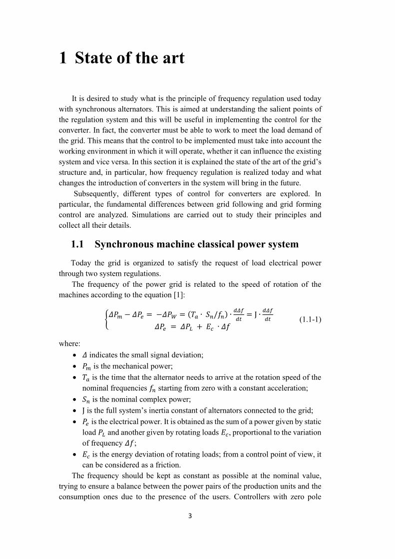
The frequency of the power grid is related to the speed of rotation of the machines according to the equation [1]

120549119875119898 minus 120549119875119890 = minus120549119875119882 = (119879119886 ∙ 119878119899119891119899) ∙

119889120549119891

119889119905= J ∙

119889120549119891

119889119905

120549119875119890 = 120549119875119871 + 119864119888 ∙ 120549119891 (11-1)

where bull 120549 indicates the small signal deviation bull 119875119898 is the mechanical power bull 119879119886 is the time that the alternator needs to arrive at the rotation speed of the

nominal frequencies 119891119899 starting from zero with a constant acceleration bull 119878119899 is the nominal complex power bull J is the full systemrsquos inertia constant of alternators connected to the grid bull 119875119890 is the electrical power It is obtained as the sum of a power given by static

load 119875119871 and another given by rotating loads 119864119888 proportional to the variation of frequency 120549119891

bull 119864119888 is the energy deviation of rotating loads from a control point of view it can be considered as a friction

The frequency should be kept as constant as possible at the nominal value trying to ensure a balance between the power pairs of the production units and the consumption ones due to the presence of the users Controllers with zero pole

4

transfer function are used but the impossibility to set a pole to zero for reasons of stability creates a non-null stedy state frequency deviation from the nominal value if rotating loads are present in the grid

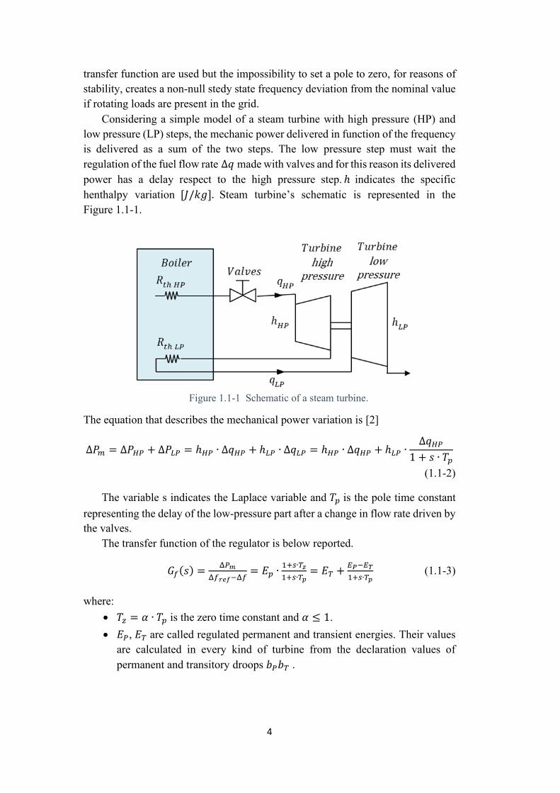
Considering a simple model of a steam turbine with high pressure (HP) and low pressure (LP) steps the mechanic power delivered in function of the frequency is delivered as a sum of the two steps The low pressure step must wait the regulation of the fuel flow rate Δ119902 made with valves and for this reason its delivered power has a delay respect to the high pressure stepℎ indicates the specific henthalpy variation [119869119896119892] Steam turbinersquos schematic is represented in the Figure 11-1

Figure 11-1 Schematic of a steam turbine

The equation that describes the mechanical power variation is [2]

Δ119875119898 = Δ119875119867119875 + Δ119875119871119875 = ℎ119867119875 ∙ Δ119902119867119875 + ℎ119871119875 ∙ Δ119902119871119875 = ℎ119867119875 ∙ Δ119902119867119875 + ℎ119871119875 ∙Δ119902119867119875

1 + 119904 ∙ 119879119901

(11-2)

The variable s indicates the Laplace variable and 119879119901 is the pole time constant representing the delay of the low-pressure part after a change in flow rate driven by the valves

The transfer function of the regulator is below reported

119866119891(119904) =Δ119875119898

Δ119891119903119890119891minusΔ119891= 119864119901 ∙

1+119904∙119879119911

1+119904∙119879119901= 119864119879 +

119864119875minus119864119879

1+119904∙119879119901 (11-3)

where bull 119879119911 = 120572 ∙ 119879119901 is the zero time constant and 120572 le 1 bull 119864119875 119864119879 are called regulated permanent and transient energies Their values

are calculated in every kind of turbine from the declaration values of permanent and transitory droops 119887119875119887119879

5

119864119875 =

119875119899

119887119875sdot119891119899

119864119879 =119875119899

119887119879sdot119891119899

119887119879 =119887119875

120572

(11-4)

The whole system is described with the following open loop transfer function

119867119874119871 = 119864119875 sdot1+119904sdot119879119911

1+119904sdot119879119875 sdot

1

119864119888+119904sdotJ (11-5)

As a goal itrsquos wanted to study what it the systems response at a load power step variation for different values of the parameters What itrsquos intention to do is to use simulation and mathematical softwares such as PLECS and MATLAB to analyse the impact that individual parameter values have on the complex system and the control dynamics Therefore itrsquos chosen to carry out simulations and calculations for a reference case using specific values for the variables After that further simulations are carried out changing one parameter at a time and making comparisons with the reference case

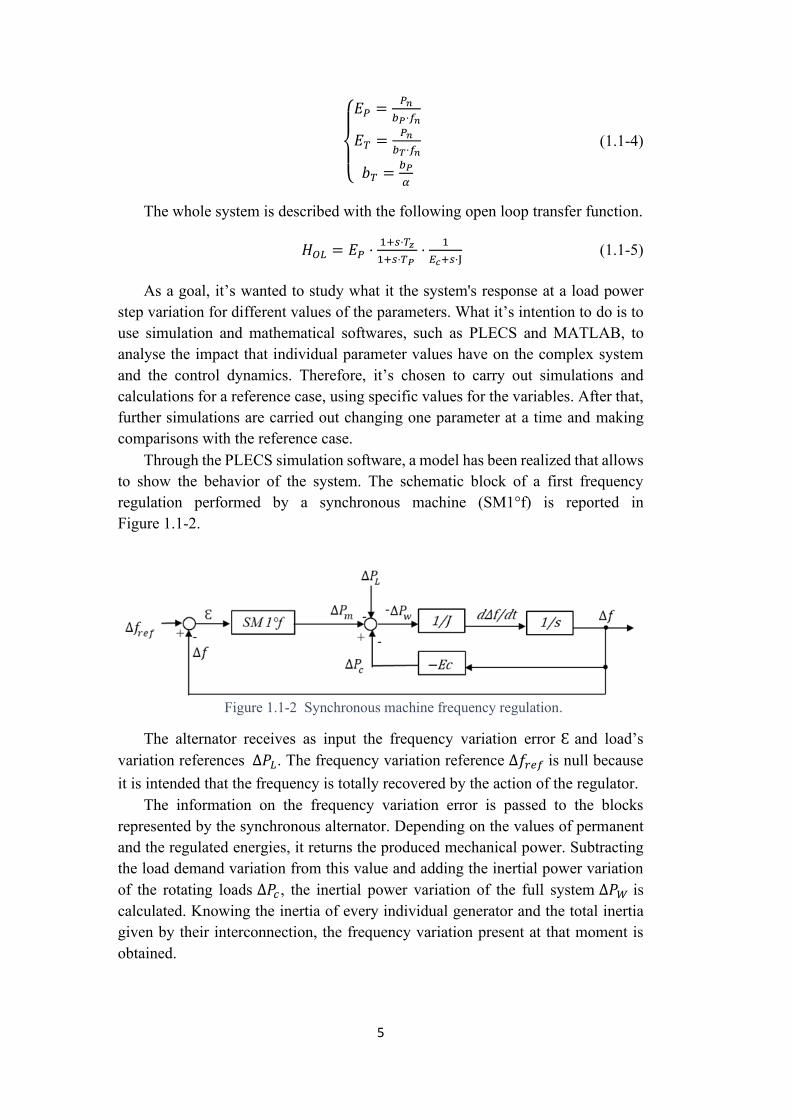
Through the PLECS simulation software a model has been realized that allows to show the behavior of the system The schematic block of a first frequency regulation performed by a synchronous machine (SM1degf) is reported in Figure 11-2

Figure 11-2 Synchronous machine frequency regulation

The alternator receives as input the frequency variation error Ɛ and loadrsquos variation references Δ119875119871 The frequency variation reference Δ119891119903119890119891 is null because it is intended that the frequency is totally recovered by the action of the regulator

The information on the frequency variation error is passed to the blocks represented by the synchronous alternator Depending on the values of permanent and the regulated energies it returns the produced mechanical power Subtracting the load demand variation from this value and adding the inertial power variation of the rotating loads Δ119875119888 the inertial power variation of the full system Δ119875119882 is calculated Knowing the inertia of every individual generator and the total inertia given by their interconnection the frequency variation present at that moment is obtained

6

The following data reported in the Table 11-1 are used as a reference It is used only a synchronous machine participating at the firts regulation of frequency (119878119872 1deg119891)

119879119886 [119904]

119879119901

[119904] 119879119911 [119904]

119864119888 [119901 119906∙ 119904]

J [ 119901 119906∙ 1199042]

12 10 25 001 024

Table 11-1 Data of the references synchronous machine

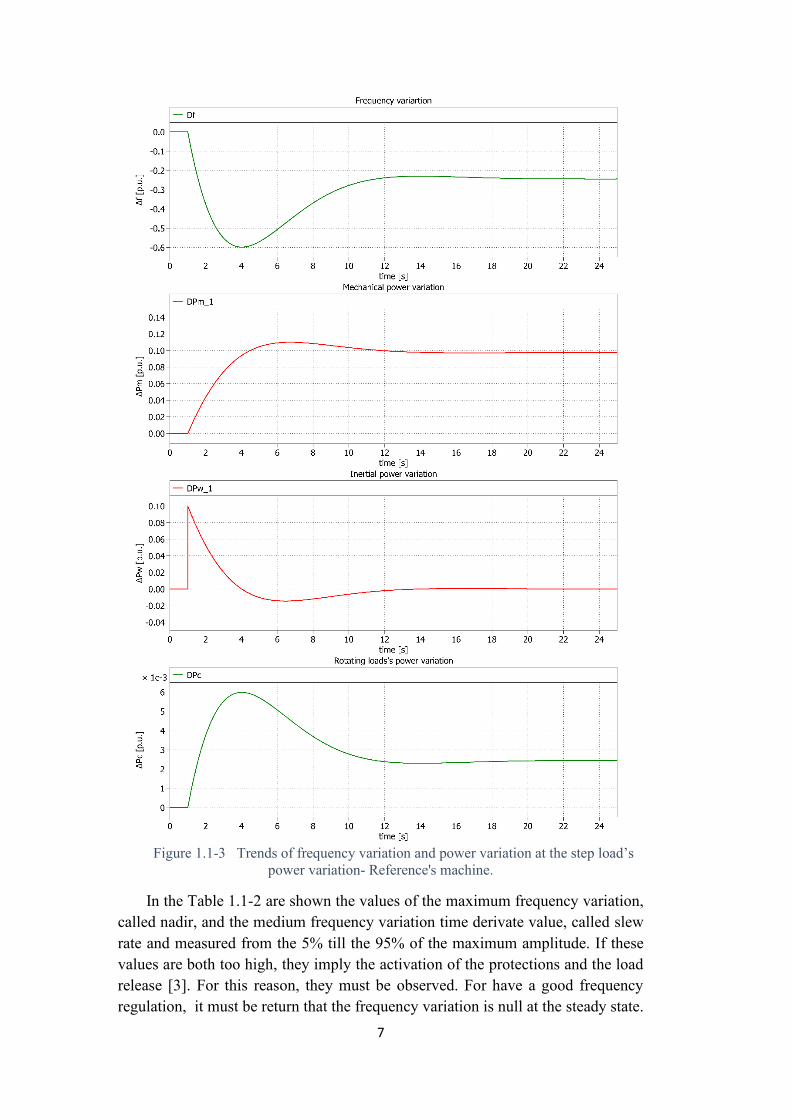
For the simulation a step of Δ119875119871 = 01 119901 119906 is applied at the time 119905 = 1 119904 The trends of frequency variation mechanical power variation provided by the controller the variation in inertial power caused by the machines and the power variation that the rotating loads have are graphed respectively in Figure 11-3

7

Figure 11-3 Trends of frequency variation and power variation at the step loadrsquos

power variation- References machine

In the Table 11-2 are shown the values of the maximum frequency variation called nadir and the medium frequency variation time derivate value called slew rate and measured from the 5 till the 95 of the maximum amplitude If these values are both too high they imply the activation of the protections and the load release [3] For this reason they must be observed For have a good frequency regulation it must be return that the frequency variation is null at the steady state

8

In this table also follow the value of the mechanical power variationrsquos overshoot and its value when the steady state condition is reched The subscript infin indicates

the steady state values

Reference data

119887119901rsquo=01

119864119905prime = 0

[119901 119906∙ 119904]

119879119911prime = 0

[119904]

120572rsquo = 0

119864119888prime = 0

[119901 119906∙ 119904]

119879119886 = 8

[119904]

119869 = 016

[ 119901 119906∙ 1199042]

Δ119891 nadir [119901 119906] -0576 -06 -0992 -0595 -0624

Δ119891 slew-rate (5)

-1545 -1599 -3877 -1663 -3071

Δ119891infin

[119901 119906 ] -0245 -046 -0245 -025 -0245

Δ119875119898 overshoot 1437 17 327 17 118

Δ119875119898infin [119901 119906] 00974 00935 00976 01 00975

Table 11-2 Dynamic results at the step loadrsquos power variation - One synchronous machine in first frequency regulation

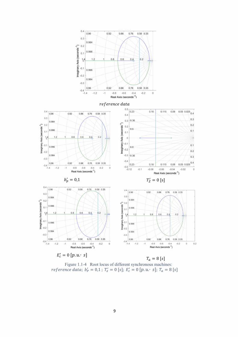
Through the study of the root locus is possible to understand how the poles of the closed-loop transfer function move compared to the open-loop ones when the gain varies For this purpose the MATLAB software data has been used The poles and damping values are shown in Figure 11-4 for the reference machine and for each test that differs for only a parameter from the reference Circles and crosses represent the position of zeros and poles of the open loop trensfer function (11-5) The blu vertical lines represent the segment connecting the closed loop poles

9

119903119890119891119890119903119890119899119888119890 119889119886119905119886

119887119901prime = 01

119879119885prime = 0 [s]

119864119888prime = 0 [119901 119906∙ 119904]

119879119886 = 8 [119904]

Figure 11-4 Root locus of different synchronous machines 119903119890119891119890119903119890119899119888119890 119889119886119905119886 119887119875

prime = 01 119879119911prime = 0 [119904] 119864119888

prime = 0 [119901 119906∙ 119904] 119879119886 = 8 [119904]

10

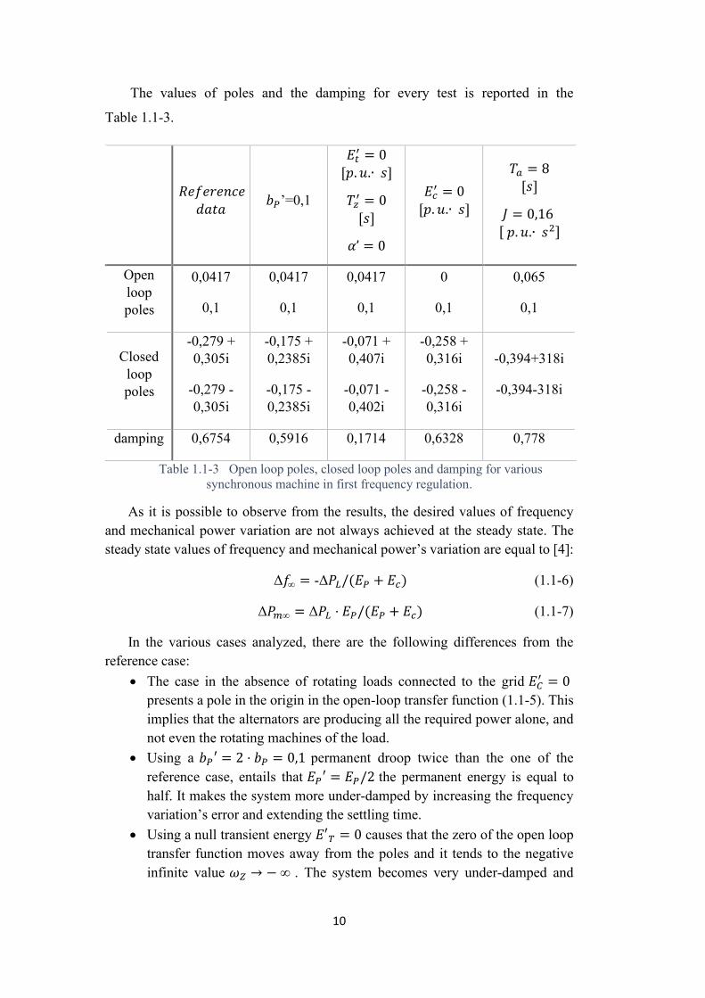
The values of poles and the damping for every test is reported in the

Table 11-3

119877119890119891119890119903119890119899119888119890

119889119886119905119886 119887119875rsquo=01

119864119905prime = 0

[119901 119906∙ 119904]

119879119911prime = 0

[119904]

120572rsquo = 0

119864119888prime = 0

[119901 119906∙ 119904]

119879119886 = 8 [119904]

119869 = 016 [ 119901 119906∙ 1199042]

Open loop poles

00417

01

00417

01

00417

01

0

01

0065

01

Closed loop poles

-0279 + 0305i

-0279 - 0305i

-0175 + 02385i

-0175 - 02385i

-0071 + 0407i

-0071 - 0402i

-0258 + 0316i

-0258 - 0316i

-0394+318i

-0394-318i

damping 06754 05916 01714 06328 0778

Table 11-3 Open loop poles closed loop poles and damping for various synchronous machine in first frequency regulation

As it is possible to observe from the results the desired values of frequency and mechanical power variation are not always achieved at the steady state The steady state values of frequency and mechanical powerrsquos variation are equal to [4]

Δ119891infin = -Δ119875119871(119864119875 + 119864119888) (11-6)

Δ119875119898infin = Δ119875119871 sdot 119864119875(119864119875 + 119864119888) (11-7)

In the various cases analyzed there are the following differences from the reference case

bull The case in the absence of rotating loads connected to the grid 119864119862prime = 0 presents a pole in the origin in the open-loop transfer function (11-5) This implies that the alternators are producing all the required power alone and not even the rotating machines of the load

bull Using a 119887119875prime = 2 sdot 119887119875 = 01 permanent droop twice than the one of the reference case entails that 119864119875prime = 1198641198752 the permanent energy is equal to half It makes the system more under-damped by increasing the frequency variationrsquos error and extending the settling time

bull Using a null transient energy 119864prime119879 = 0 causes that the zero of the open loop transfer function moves away from the poles and it tends to the negative infinite value 120596119885 rarr minus infin The system becomes very under-damped and

11

oscillating The overshoot of the Δ119875119898 mechanical power variation and the Δ119891 frequency variation derivatives become very large

bull Using a lower J inertia value causes the root locus poles to move away from the origin and increasing the systems damping There are curves with much larger derivatives and during the load take-off the frequency variation is more relevant The power variationrsquos overshoot is reduced because with a shorter start time it is faster to reach the nominal speed

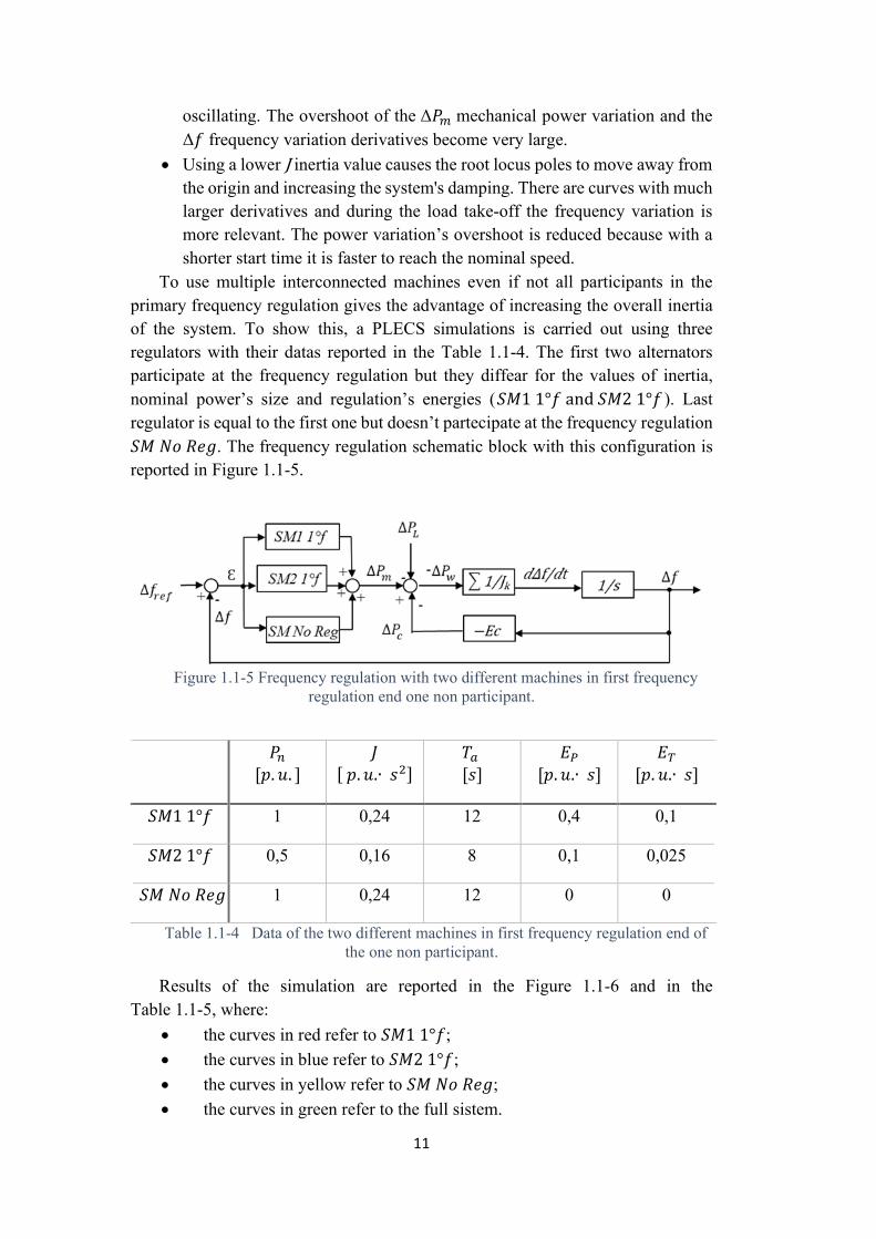
To use multiple interconnected machines even if not all participants in the primary frequency regulation gives the advantage of increasing the overall inertia of the system To show this a PLECS simulations is carried out using three regulators with their datas reported in the Table 11-4 The first two alternators participate at the frequency regulation but they diffear for the values of inertia nominal powerrsquos size and regulationrsquos energies (1198781198721 1deg119891 and 1198781198722 1deg119891 ) Last regulator is equal to the first one but doesnrsquot partecipate at the frequency regulation 119878119872 119873119900 119877119890119892 The frequency regulation schematic block with this configuration is reported in Figure 11-5

Figure 11-5 Frequency regulation with two different machines in first frequency

regulation end one non participant

119875119899

[119901 119906 ] 119869

[ 119901 119906∙ 1199042] 119879119886

[119904] 119864119875

[119901 119906∙ 119904] 119864119879

[119901 119906∙ 119904]

1198781198721 1deg119891 1 024 12 04 01

1198781198722 1deg119891 05 016 8 01 0025

119878119872 119873119900 119877119890119892 1 024 12 0 0

Table 11-4 Data of the two different machines in first frequency regulation end of the one non participant

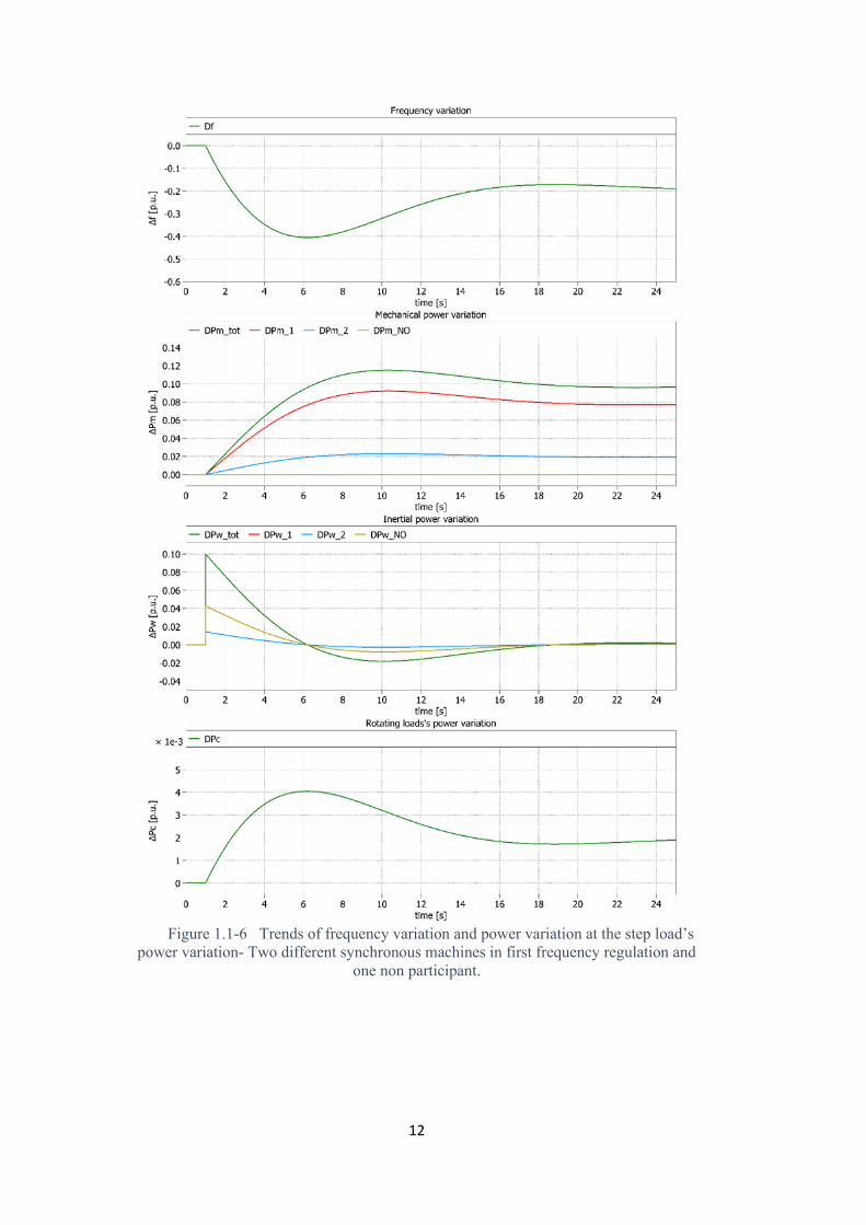
Results of the simulation are reported in the Figure 11-6 and in the Table 11-5 where

bull the curves in red refer to 1198781198721 1deg119891 bull the curves in blue refer to 1198781198722 1deg119891 bull the curves in yellow refer to 119878119872 119873119900 119877119890119892 bull the curves in green refer to the full sistem

12

Figure 11-6 Trends of frequency variation and power variation at the step loadrsquos

power variation- Two different synchronous machines in first frequency regulation and one non participant

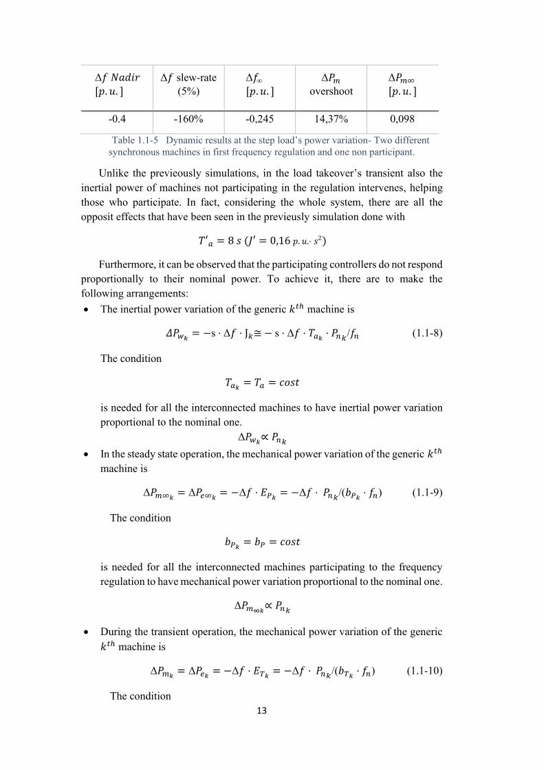
13

Δ119891 119873119886119889119894119903

[119901 119906 ] Δ119891 slew-rate

(5) Δ119891infin

[119901 119906 ] Δ119875119898

overshoot Δ119875119898infin

[119901 119906 ]

-04 -160 -0245 1437 0098

Table 11-5 Dynamic results at the step loadrsquos power variation- Two different synchronous machines in first frequency regulation and one non participant

Unlike the previeously simulations in the load takeoverrsquos transient also the inertial power of machines not participating in the regulation intervenes helping those who participate In fact considering the whole system there are all the opposit effects that have been seen in the previeusly simulation done with

119879prime119886 = 8 119904 (119869prime = 016 119901 119906sdot 1199042)

Furthermore it can be observed that the participating controllers do not respond proportionally to their nominal power To achieve it there are to make the following arrangements bull The inertial power variation of the generic 119896119905ℎ machine is

120549119875119908119896 = minuss sdot Δ119891 sdot J119896congminus s sdot Δ119891 sdot 119879119886119896 sdot 119875119899119896119891119899 (11-8)

The condition

119879119886119896 = 119879119886 = 119888119900119904119905

is needed for all the interconnected machines to have inertial power variation proportional to the nominal one Δ119875119908119896prop 119875119899119896

bull In the steady state operation the mechanical power variation of the generic 119896119905ℎ machine is

Δ119875119898infin119896= Δ119875119890infin119896

= minusΔ119891 sdot 119864119875119896 = minusΔ119891 sdot 119875119899119896(119887119875119896 sdot 119891119899) (11-9)

The condition

119887119875119896 = 119887119875 = 119888119900119904119905

is needed for all the interconnected machines participating to the frequency regulation to have mechanical power variation proportional to the nominal one

Δ119875119898infin119896prop 119875119899119896

bull During the transient operation the mechanical power variation of the generic 119896119905ℎ machine is

Δ119875119898119896= Δ119875119890119896 = minusΔ119891 sdot 119864119879119896 = minusΔ119891 sdot 119875119899119896(119887119879119896 sdot 119891119899) (11-10)

The condition

14

119887119879119896 = 119887119879 = 119888119900119904119905

is needed for all the interconnected machines participating to the frequency regulation to have mechanical power variation proportional to the nominal one

Δ119875119898119896prop 119875119899119896

Overall there is a non-zero error on the frequencyrsquos variation at the steady

state Using a pole transfer function would originally give zero error at the steady

state but achieving this is prevented by the fact that the distribution of the primary control on multiple units would be indeterminate

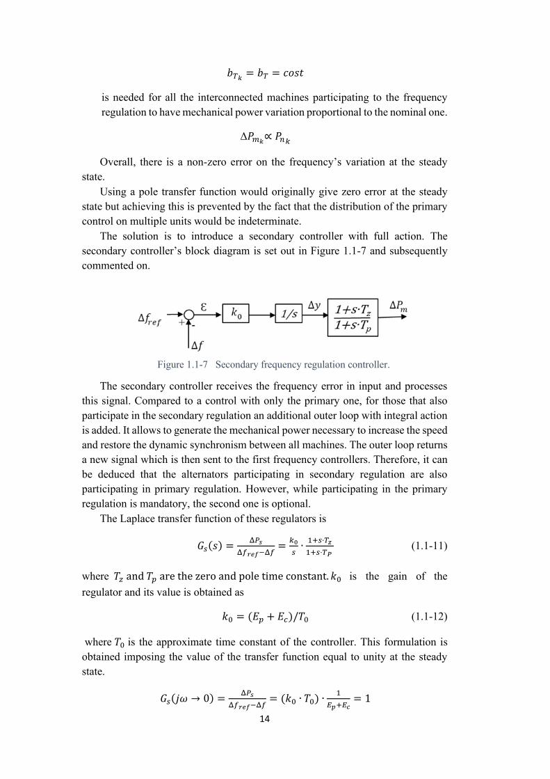
The solution is to introduce a secondary controller with full action The secondary controllerrsquos block diagram is set out in Figure 11-7 and subsequently commented on

Figure 11-7 Secondary frequency regulation controller

The secondary controller receives the frequency error in input and processes this signal Compared to a control with only the primary one for those that also participate in the secondary regulation an additional outer loop with integral action is added It allows to generate the mechanical power necessary to increase the speed and restore the dynamic synchronism between all machines The outer loop returns a new signal which is then sent to the first frequency controllers Therefore it can be deduced that the alternators participating in secondary regulation are also participating in primary regulation However while participating in the primary regulation is mandatory the second one is optional

The Laplace transfer function of these regulators is

119866119904(119904) =Δ119875119904

Δ119891119903119890119891minusΔ119891=

1198960

119904∙1+119904sdot119879119911

1+119904sdot119879119875 (11-11)

where 119879119911 and 119879119901 are the zero and pole time constant 1198960 is the gain of the regulator and its value is obtained as

1198960 = (119864119901 + 119864119888)1198790 (11-12)

where 1198790 is the approximate time constant of the controller This formulation is obtained imposing the value of the transfer function equal to unity at the steady state

119866119904(119895120596 rarr 0) =Δ119875119904

Δ119891119903119890119891minusΔ119891= (1198960 ∙ 1198790) ∙

1

119864119901+119864119888= 1

15

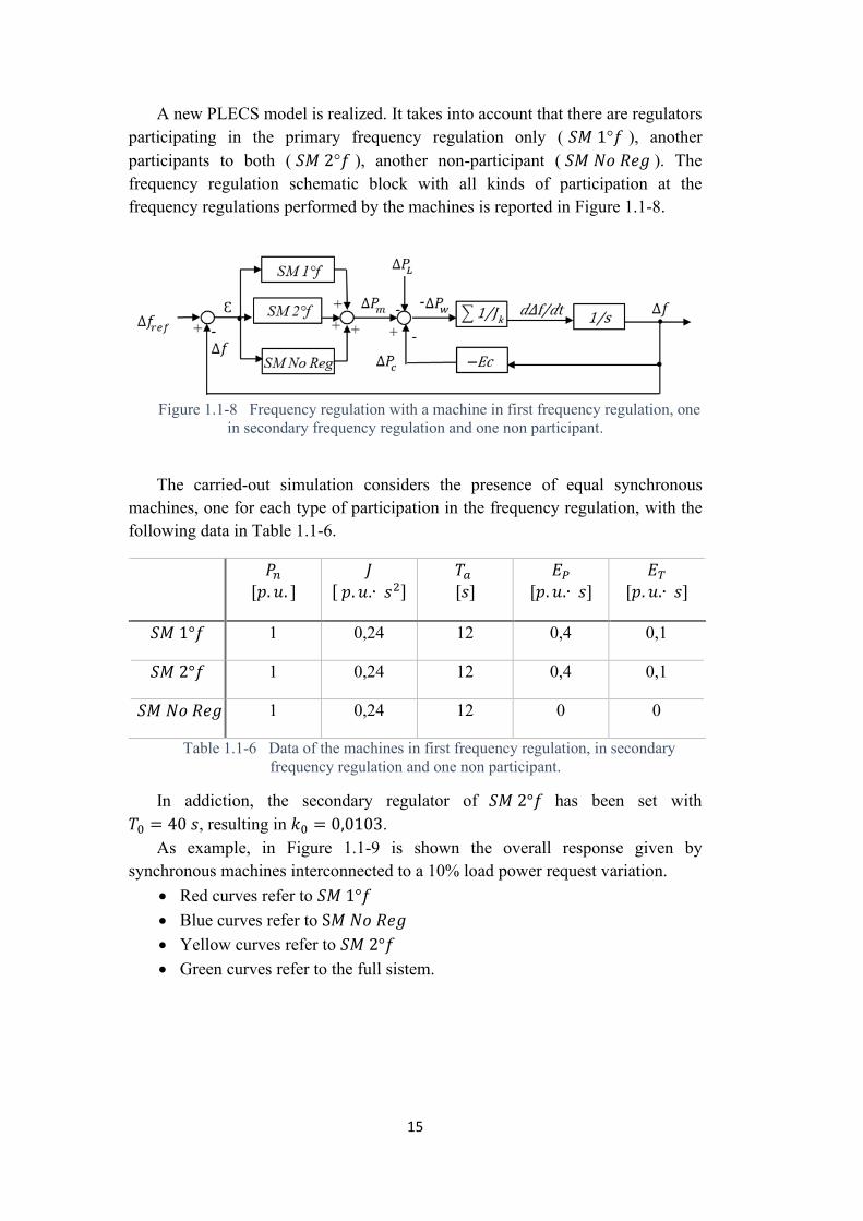
A new PLECS model is realized It takes into account that there are regulators participating in the primary frequency regulation only ( 119878119872 1deg119891 ) another participants to both ( 119878119872 2deg119891 ) another non-participant ( 119878119872 119873119900 119877119890119892 ) The frequency regulation schematic block with all kinds of participation at the frequency regulations performed by the machines is reported in Figure 11-8

Figure 11-8 Frequency regulation with a machine in first frequency regulation one

in secondary frequency regulation and one non participant

The carried-out simulation considers the presence of equal synchronous

machines one for each type of participation in the frequency regulation with the following data in Table 11-6

119875119899 [119901 119906 ]

119869 [ 119901 119906∙ 1199042]

119879119886 [119904]

119864119875 [119901 119906∙ 119904]

119864119879 [119901 119906∙ 119904]

119878119872 1deg119891 1 024 12 04 01

119878119872 2deg119891 1 024 12 04 01

119878119872 119873119900 119877119890119892 1 024 12 0 0

Table 11-6 Data of the machines in first frequency regulation in secondary frequency regulation and one non participant

In addiction the secondary regulator of 119878119872 2deg119891 has been set with 1198790 = 40 119904 resulting in 1198960 = 00103

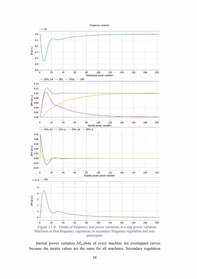
As example in Figure 11-9 is shown the overall response given by synchronous machines interconnected to a 10 load power request variation

bull Red curves refer to 119878119872 1deg119891 bull Blue curves refer to S119872 119873119900 119877119890119892 bull Yellow curves refer to 119878119872 2deg119891 bull Green curves refer to the full sistem

16

Figure 11-9 Trends of frequency and power variations at a step power variation -

Machines in first frequency regulation in secondary frequency regulation and non-participant

Inertial power variation Δ119875119908 plots of every machine are overlapped curves because the inertia values are the same for all machines Secondary regulation

17

mainly works at the steady state by replacing the primary regulation The transitory trend remains almost unchanged The frequency and mechanical power variation of the system at the steady state are

120549119891infin = 0

Δ119875119898infin=Δ119875119871 + 119864119888 sdot Δ119891 = Δ119875119871 (11-13)

and the mechanical power provided by the alternators is

Δ119875119875infin = minus119864119875 middot Δ119891 = 0Δ119875119878infin=Δ119875119898-Δ119875119875 = Δ119875119871

(11-14)

In the first moments the load variation Δ119875119871 is fed by the inertial power of all interconnected machines The frequency decreases and generates a speed error compared to the reference (synchronization frequency) The first response action is the primary regulation but this cannot compensate the whole load request because of the disturbance caused by the rotating loads The integral action of the controller participating in the secondary regulation leads to the cancellation of the frequency variationrsquos error by restoring the reference frequency and the synchronism between all the machines by delivering the proper value of mechanical power Through a slower dynamic it replaces the primary regulation

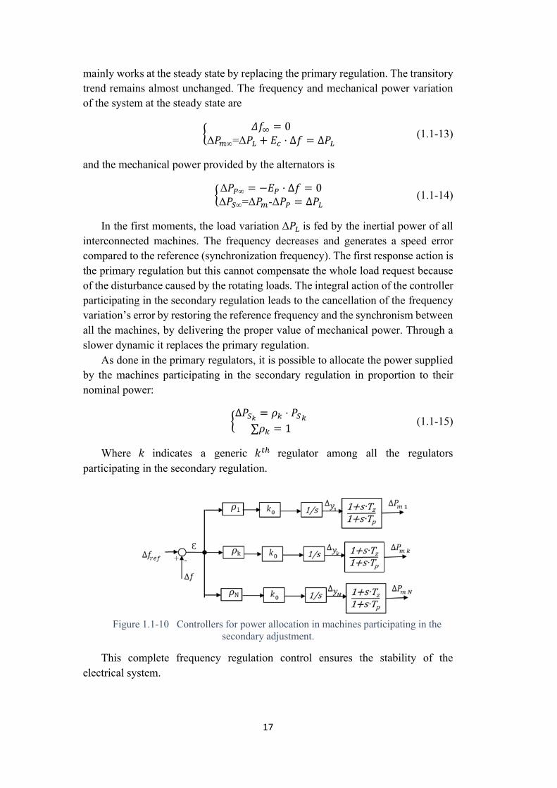
As done in the primary regulators it is possible to allocate the power supplied by the machines participating in the secondary regulation in proportion to their nominal power

Δ119875119878119896 = 120588119896 sdot 119875119878119896

sum120588119896 = 1 (11-15)

Where 119896 indicates a generic 119896119905ℎ regulator among all the regulators participating in the secondary regulation

Figure 11-10 Controllers for power allocation in machines participating in the

secondary adjustment

This complete frequency regulation control ensures the stability of the electrical system

18

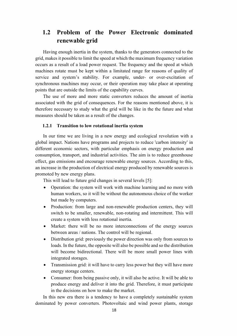
12 Problem of the Power Electronic dominated renewable grid

Having enough inertia in the system thanks to the generators connected to the grid makes it possible to limit the speed at which the maximum frequency variation occurs as a result of a load power request The frequency and the speed at which machines rotate must be kept within a limitated range for reasons of quality of service and systemrsquos stability For example under- or over-excitation of synchronous machines may occur or their operation may take place at operating points that are outside the limits of the capability curves

The use of more and more static converters reduces the amount of inertia associated with the grid of consequences For the reasons mentioned above it is therefore necessary to study what the grid will be like in the the future and what measures should be taken as a result of the changes

121 Transition to low rotational inertia system

In our time we are living in a new energy and ecological revolution with a global impact Nations have programs and projects to reduce carbon intensity in different economic sectors with particular emphasis on energy production and consumption transport and industrial activities The aim is to reduce greenhouse effect gas emissions and encourage renewable energy sources According to this an increase in the production of electrical energy produced by renewable sources is promoted by new energy plans

This will lead to future grid changes in several levels [5] bull Operation the system will work with machine learning and no more with

human workers so it will be without the autonomous choice of the worker but made by computers

bull Production from large and non-renewable production centers they will switch to be smaller renewable non-rotating and intermittent This will create a system with less rotational inertia

bull Market there will be no more interconnections of the energy sources between areas nations The control will be regional

bull Distribution grid previously the power direction was only from sources to loads In the future the opposite will also be possible and so the distribution will become bidirectional There will be more small power lines with integrated storages

bull Transmission grid it will have to carry less power but they will have more energy storage centers

bull Consumer from being passive only it will also be active It will be able to produce energy and deliver it into the grid Therefore it must participate in the decisions on how to make the market

In this new era there is a tendency to have a completely sustainable system dominated by power converters Photovoltaic and wind power plants storage

19

systems residential and industrial utilities all points on the grid from loads to production will need the presence of an electronic power converter It is therefore necessary to take into account all the consequences that this transition has on the power system and how its dynamic response changes The System Non-Synchronous Penetration index (119878119873119878119875) has been introduced to assess how far the power converter penetrated It is defined in [6]

119878119873119878119875 =119875119899119900119899minus119904119910119899119888ℎ119903119900119899119900119906119904 119901119903119900119889119906119888119905119894119900119899 + 119875119894119899119905119890119903119888119900119899119899119890119888119905119894119900119899

119875119897119900119886119889+119875119890119909119901119900119903119905119890119889 119908119894119905ℎ 119894119899119905119890119903119888119900119899119899119890119888119905119894119900119899 (12-1)

where 119875 indicates the power in W This index is the ratio of the real time power contribution of the non-

synchronous production and the net import of the loads plus the net exports In the past with few power converters installed the index was very low and not

many situations with little equivalent inertia were measured Therefore the safe operation of the system was assured After 50 of renewable energy produced the system starts to have high penetration of nonrsquosynchronous production and there is the risk of no-safety of the electrical system Nowadays if the level of the 75 is exceeded the renewable sources are disconnected

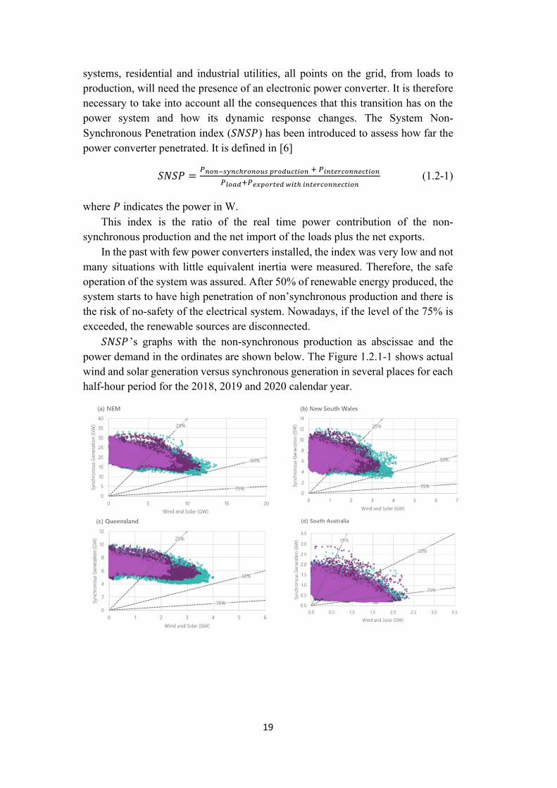
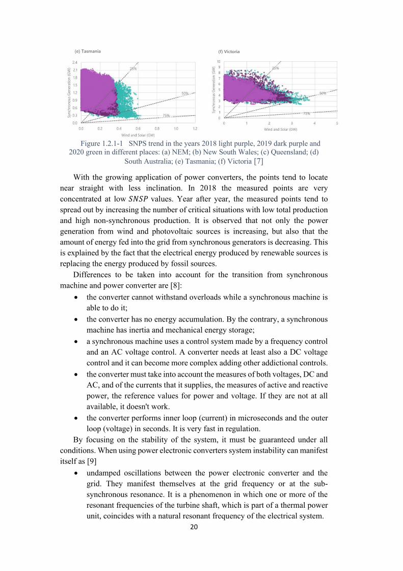
119878119873119878119875 rsquos graphs with the non-synchronous production as abscissae and the power demand in the ordinates are shown below The Figure 121-1 shows actual wind and solar generation versus synchronous generation in several places for each half-hour period for the 2018 2019 and 2020 calendar year

20

Figure 121-1 SNPS trend in the years 2018 light purple 2019 dark purple and

2020 green in different places (a) NEM (b) New South Wales (c) Queensland (d) South Australia (e) Tasmania (f) Victoria [7]

With the growing application of power converters the points tend to locate near straight with less inclination In 2018 the measured points are very concentrated at low 119878119873119878119875 values Year after year the measured points tend to spread out by increasing the number of critical situations with low total production and high non-synchronous production It is observed that not only the power generation from wind and photovoltaic sources is increasing but also that the amount of energy fed into the grid from synchronous generators is decreasing This is explained by the fact that the electrical energy produced by renewable sources is replacing the energy produced by fossil sources

Differences to be taken into account for the transition from synchronous machine and power converter are [8]

bull the converter cannot withstand overloads while a synchronous machine is able to do it

bull the converter has no energy accumulation By the contrary a synchronous machine has inertia and mechanical energy storage

bull a synchronous machine uses a control system made by a frequency control and an AC voltage control A converter needs at least also a DC voltage control and it can become more complex adding other addictional controls

bull the converter must take into account the measures of both voltages DC and AC and of the currents that it supplies the measures of active and reactive power the reference values for power and voltage If they are not at all available it doesnt work

bull the converter performs inner loop (current) in microseconds and the outer loop (voltage) in seconds It is very fast in regulation

By focusing on the stability of the system it must be guaranteed under all conditions When using power electronic converters system instability can manifest itself as [9]

bull undamped oscillations between the power electronic converter and the grid They manifest themselves at the grid frequency or at the sub-synchronous resonance It is a phenomenon in which one or more of the resonant frequencies of the turbine shaft which is part of a thermal power unit coincides with a natural resonant frequency of the electrical system

21

bull loss of synchronism is possible for power converter-based technologies This could be due to an inertia not adequately defined Virtual inertia is generated by storage systems associated with inverters to keep the rate of frequency variation low in case of active power imbalances especially under sub-frequency conditions

bull loss of fault ride through capability Synchronous generators can slip and become unstable if the stator voltage drops below a certain threshold When a voltage drop occurs even a power converter can become unstable

The cause may be due to the incorrect converter control interacting with the grid [10]

While with synchronous machine the stability is guaranteed ensuring the rotor angle stability the frequency stability and the voltage stability using power converter the power systemrsquos stability is obtained by the stability of resonance and

the converter driven stability [11]

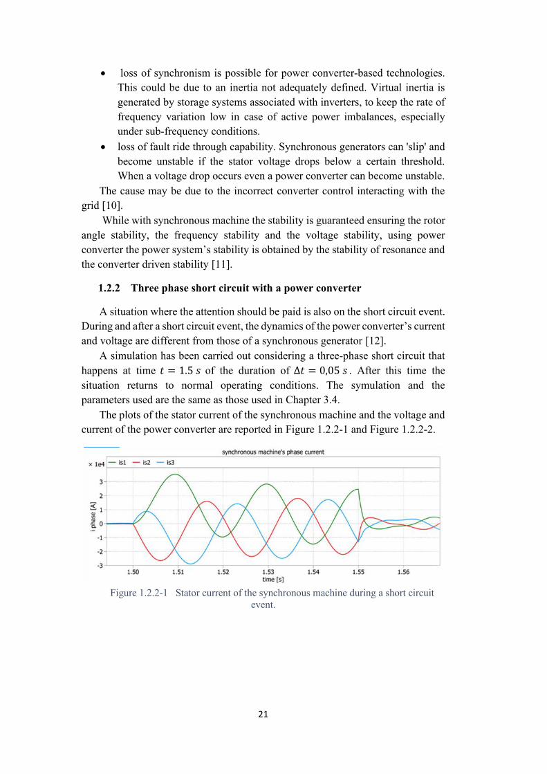
122 Three phase short circuit with a power converter

A situation where the attention should be paid is also on the short circuit event During and after a short circuit event the dynamics of the power converterrsquos current

and voltage are different from those of a synchronous generator [12] A simulation has been carried out considering a three-phase short circuit that

happens at time 119905 = 15 119904 of the duration of Δ119905 = 005 119904 After this time the situation returns to normal operating conditions The symulation and the parameters used are the same as those used in Chapter 34

The plots of the stator current of the synchronous machine and the voltage and current of the power converter are reported in Figure 122-1 and Figure 122-2

Figure 122-1 Stator current of the synchronous machine during a short circuit

event

22

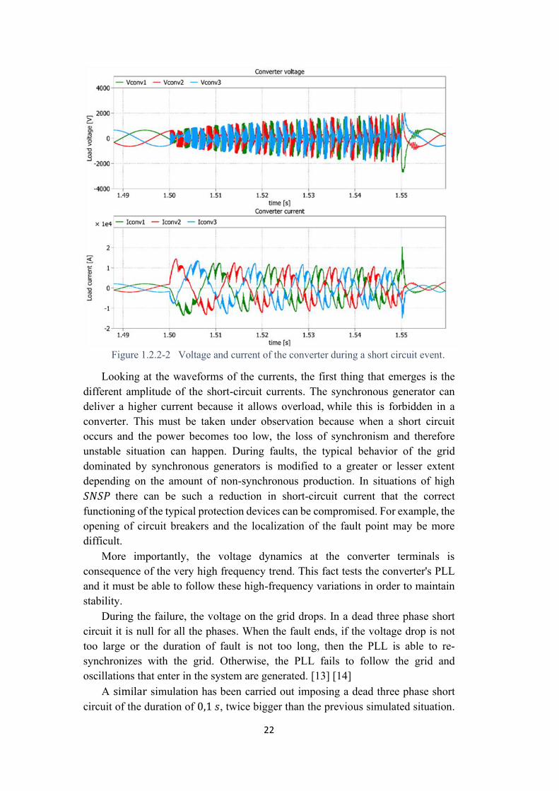
Figure 122-2 Voltage and current of the converter during a short circuit event

Looking at the waveforms of the currents the first thing that emerges is the different amplitude of the short-circuit currents The synchronous generator can deliver a higher current because it allows overload while this is forbidden in a converter This must be taken under observation because when a short circuit occurs and the power becomes too low the loss of synchronism and therefore unstable situation can happen During faults the typical behavior of the grid dominated by synchronous generators is modified to a greater or lesser extent depending on the amount of non-synchronous production In situations of high 119878119873119878119875 there can be such a reduction in short-circuit current that the correct functioning of the typical protection devices can be compromised For example the opening of circuit breakers and the localization of the fault point may be more difficult

More importantly the voltage dynamics at the converter terminals is consequence of the very high frequency trend This fact tests the converters PLL and it must be able to follow these high-frequency variations in order to maintain stability

During the failure the voltage on the grid drops In a dead three phase short circuit it is null for all the phases When the fault ends if the voltage drop is not too large or the duration of fault is not too long then the PLL is able to re-synchronizes with the grid Otherwise the PLL fails to follow the grid and oscillations that enter in the system are generated [13] [14]

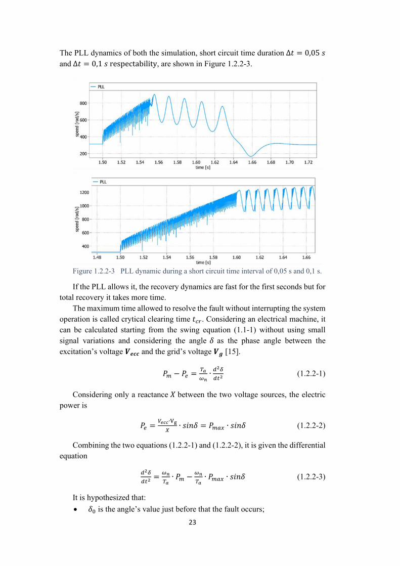
A similar simulation has been carried out imposing a dead three phase short circuit of the duration of 01 119904 twice bigger than the previous simulated situation

23

The PLL dynamics of both the simulation short circuit time duration Δ119905 = 005 119904 and Δ119905 = 01 119904 respectability are shown in Figure 122-3

Figure 122-3 PLL dynamic during a short circuit time interval of 005 s and 01 s

If the PLL allows it the recovery dynamics are fast for the first seconds but for total recovery it takes more time

The maximum time allowed to resolve the fault without interrupting the system operation is called crytical clearing time 119905119888119903 Considering an electrical machine it can be calculated starting from the swing equation (11-1) without using small signal variations and considering the angle 120575 as the phase angle between the excitationrsquos voltage 119933119942119940119940 and the gridrsquos voltage 119933119944 [15]

119875119898 minus 119875119890 =119879119886

120596119899∙1198892120575

1198891199052 (122-1)

Considering only a reactance 119883 between the two voltage sources the electric power is

119875119890 =119881119890119888119888∙Vg

119883∙ 119904119894119899120575 = 119875119898119886119909 ∙ 119904119894119899120575 (122-2)

Combining the two equations (122-1) and (122-2) it is given the differential equation

1198892120575

1198891199052=

120596119899

119879119886∙ 119875119898 minus

120596119899

119879119886∙ 119875119898119886119909 ∙ 119904119894119899120575 (122-3)

It is hypothesized that bull 1205750 is the anglersquos value just before that the fault occurs

24

bull 119875119890 is null during the fault bull there is the critical clearing angle 120575119888119903 after the fault The system remains stable if the fault is solved before this time or if the angle

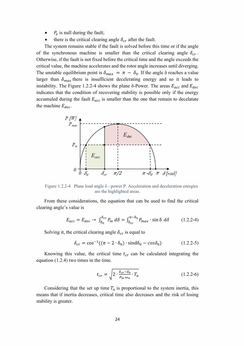
of the synchronous machine is smaller than the critical clearing angle 120575119888119903 Otherwise if the fault is not fixed before the critical time and the angle exceeds the critical value the machine accelerates and the rotor angle increases until diverging The unstable equilibrium point is 120575119898119886119909 = 120587 minus 1205750 If the angle δ reaches a value larger than 120575119898119886119909 there is insufficient decelerating energy and so it leads to instability The Figure 122-4 shows the plane δ-Power The areas 119864119886119888119888 and 119864119889119890119888 indicates that the condition of recovering stability is possible only if the energy accumuled during the fault 119864119886119888119888 is smaller than the one that remain to decelatate the machine 119864119889119890119888

Figure 122-4 Plane load angle δ - power P Acceleration and deceleration energies are the highlighted areas

From these considerations the equation that can be used to find the critical clearing anglersquos value is

119864119886119888119888 = 119864119889119890119888 rarr int 119875119898 119889120575δ119888119903δ0

= int 119875119898119886119909 ∙ sin δ 119889120575πminusδ0δcr

(122-4)

Solving it the critical clearing angle 120575119888119903 is equal to

120575119888119903 = cosminus1((120587 minus 2 ∙ δ0) ∙ sindδ0 minus 1198881199001199041205750) (122-5)

Knowing this value the critical time 119905119888119903 can be calculated integrating the equation (124) two times in the time

119905119888119903 = radic2 ∙120575119888119903minus1205750

119875119898∙120596119899∙ 119879119886 (122-6)

Considering that the set up time 119879119886 is proportional to the system inertia this means that if inertia decreases critical time also decreases and the risk of losing stability is greater

25

In addition reconsidering the equation (122-2) and using small signal variation it becames

Δ119875119890 = 119875119898119886119909 ∙ 1198881199001199041205750 ∙ Δ120575 (122-7)

Let introduce an asynchronous power 119875119886119904 term of the damping windings as consequence of the currents that flow in the rotor induced by the stator Itrsquos

proportional to the change in speed from 1205960 when the fault occurs by the damping coefficient 119863[16]

119875119886119904 = 119863 ∙ (1205960 minus 120596) = minus119863

120596119899∙119889120575

119889119905 (122-8)

The systemrsquos differential equation in small variation signals is

Δ119875119898 = Δ119875119890 minus Δ119875119886119904 +119879119886

120596119899∙119889Δ120596

119889119905= 119875119898119886119909 ∙ 1198881199001199041205750 ∙ Δ120575 +

119863

120596119899∙119889Δ120575

119889119905+ 119879119886 ∙

1198892Δ120575

1198891199052

(122-9)

In control matrix form the system is expressed as

119889

119889119905[Δ120596Δ120575] = [

minus119863

119879119886minus119875119898119886119909 ∙ 1198881199001199041205750119879119886

120596119899 0] ∙ [

Δ120596Δ120575] + [

Δ1198751198980] (122-10)

Eigenvalues are derived from the state matrix Det(_) indicates the determinant operator applied to the matrix between the brackets

Det([minus119863

119879119886minus 119901 minus119875119898119886119909 ∙ 1198881199001199041205750119879119886

120596119899 minus119901]) = 1199012 minus

119863

119879119886∙ 119901 + 120596119899 ∙

119875119898119886119909∙1198881199001199041205750

119879119886= 0

119901plusmn = minus119863

119879119886plusmn 119895radic

119875119898119886119909∙cos1205750∙120596119899

Taminus (

119863

2∙119879119886)2

(122-11)

Reducing inertia the damping 120577 and the natural frequency of the mechanical motion 120596119899119886119905 increase

120596119899119886119905 = radic119875119898119886119909∙cos1205750∙120596

Ta (122-12)

120577 =minus119863

119879119886

2∙radic119875119898119886119909∙cos1205750∙120596

Ta

(122-13)

The result is that by decreasing inertia the synchronous machines decelerate faster reaching a lower minimum frequency (nadir)

26

123 Short and long term solutions

To solve problems that come from the power converters high penetration in the grid its possible to take some measures

There are short-term solutions and long-term solutions Some of them are listed in Table 123-1 [17]

Short-term solutions Long-term solutions

bull Grid connection codes bull Mitigation measures bull Ancillary services bull Synchronous condenser

bull Synthetic inertia bull Grid forming control

advanced use of storages or HVDC

Table 123-1 Short-term solutions and long-term solutions for low inertia systems

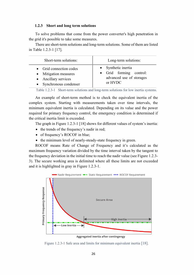
An example of short-term method is to check the equivalent inertia of the complex system Starting with measurements taken over time intervals the minimum equivalent inertia is calculated Depending on its value and the power required for primary frequency control the emergency condition is determined if the critical inertia limit is exceeded

The graph in Figure 123-1 [18] shows for different values of systemrsquos inertia bull the trends of the frequencyrsquos nadir in red bull of frequencyrsquos ROCOF in blue bull the minimum level of nearly-steady-state frequency in green ROCOF means Rate of Change of Frequency and itrsquos calculated as the

maximum frequency variation divided by the time interval taken by the tangent to the frequency deviation in the initial time to reach the nadir value (see Figure 123-3) The secure working area is delimited where all these limits are not exceeded and it is highlighted in gray in Figure 123-1

Figure 123-1 Safe area and limits for minimum equivalent inertia [18]

27

The conditions of minimum total inertia are determined by an acceptable limit of nadir frequency ROCOF and power demand When leaving the safe area protections are activated to return to acceptable inertia conditions

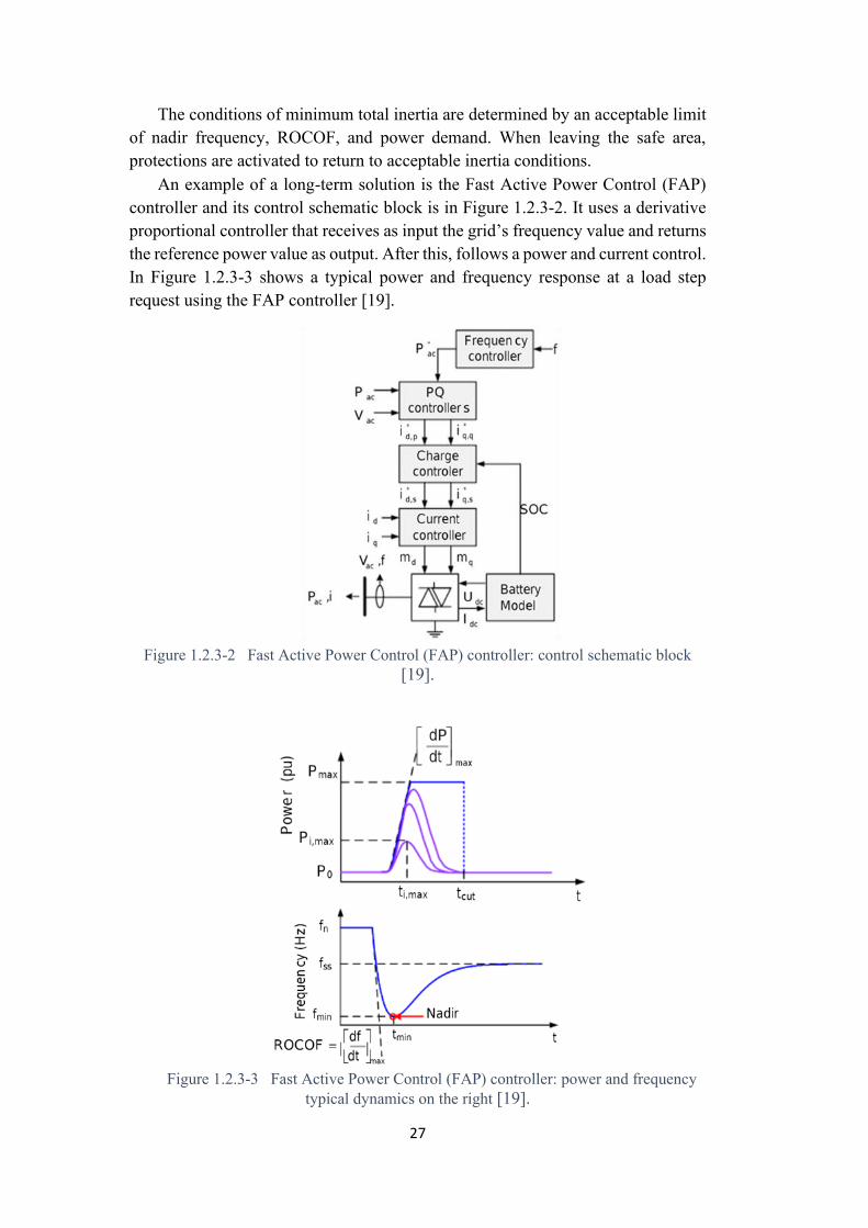
An example of a long-term solution is the Fast Active Power Control (FAP) controller and its control schematic block is in Figure 123-2 It uses a derivative proportional controller that receives as input the gridrsquos frequency value and returns the reference power value as output After this follows a power and current control In Figure 123-3 shows a typical power and frequency response at a load step request using the FAP controller [19]

Figure 123-2 Fast Active Power Control (FAP) controller control schematic block

[19]

Figure 123-3 Fast Active Power Control (FAP) controller power and frequency

typical dynamics on the right [19]

28

The proportional coefficient 119896119901 can have a dead band to keep the power constant in that frequency range and saturators for the maximum bidirectional power

The derivative coefficient 119896119889 determinates the ROCOF [20]

Δ119875 = 119896119889 ∙119889119891(119905)

119889119905 (123-1)

Its value is chosen so that applying a frequency pulse 119891119898119894119899 minus 119891119899 a power variation of Δ119875 = 119875119898119886119909 minus 1198750 is generated

With these considerations in mind a closer look at the possible control strategies for power converters in the grid is given in the next sub-chapters

13 Grid following and grid forming

In a future low-inertia power system the functionalities of the frequency regulation must be provided by an appropriate control of the converters operation

In this sub-chapter two possible control strategies for converters connected to the grid are compared and evaluated Then the work continues looking for how to realize one for the project converter

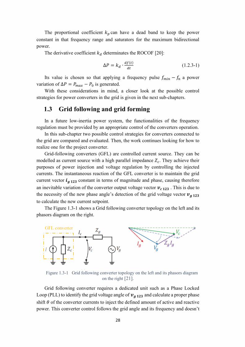
Grid-following converters (GFL) are controlled current source They can be modelled as current source with a high parallel impedance 119885119888 They achieve their purposes of power injection and voltage regulation by controlling the injected currents The instantaneous reaction of the GFL converter is to maintain the grid current vector 119946119944 120783120784120785 constant in terms of magnitude and phase causing therefore an inevitable variation of the converter output voltage vector 119959119940 120783120784120785 This is due to the necessity of the new phase anglersquos detection of the grid voltage vector 119959119944 120783120784120785 to calculate the new current setpoint

The Figure 13-1 shows a Grid following converter topology on the left and its phasors diagram on the right

Figure 13-1 Grid following converter topology on the left and its phasors diagram on the right [21]

Grid following converter requires a dedicated unit such as a Phase Locked Loop (PLL) to identify the grid voltage angle of 119959119944 120783120784120785 and calculate a proper phase shift 120579 of the converter currents to inject the defined amount of active and reactive power This converter control follows the grid angle and its frequency and doesnrsquot

29

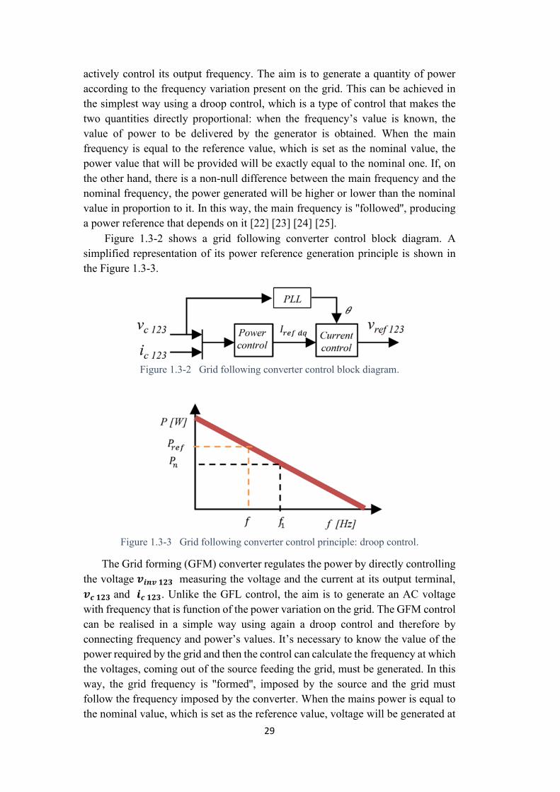
actively control its output frequency The aim is to generate a quantity of power according to the frequency variation present on the grid This can be achieved in the simplest way using a droop control which is a type of control that makes the two quantities directly proportional when the frequencyrsquos value is known the value of power to be delivered by the generator is obtained When the main frequency is equal to the reference value which is set as the nominal value the power value that will be provided will be exactly equal to the nominal one If on the other hand there is a non-null difference between the main frequency and the nominal frequency the power generated will be higher or lower than the nominal value in proportion to it In this way the main frequency is followed producing a power reference that depends on it [22] [23] [24] [25]

Figure 13-2 shows a grid following converter control block diagram A simplified representation of its power reference generation principle is shown in the Figure 13-3

Figure 13-2 Grid following converter control block diagram

Figure 13-3 Grid following converter control principle droop control

The Grid forming (GFM) converter regulates the power by directly controlling the voltage 119959119946119951119959 120783120784120785 measuring the voltage and the current at its output terminal 119959119940 120783120784120785 and 119946119940 120783120784120785 Unlike the GFL control the aim is to generate an AC voltage with frequency that is function of the power variation on the grid The GFM control can be realised in a simple way using again a droop control and therefore by connecting frequency and powerrsquos values Itrsquos necessary to know the value of the power required by the grid and then the control can calculate the frequency at which the voltages coming out of the source feeding the grid must be generated In this way the grid frequency is formed imposed by the source and the grid must follow the frequency imposed by the converter When the mains power is equal to the nominal value which is set as the reference value voltage will be generated at

30

exactly the nominal frequency If on the other hand the main power varies and therefore differs from the nominal value the frequency at which the voltages are generated will be bigger or smaller than the nominal value depending on this difference For example in the case droop control they will be proportional as in Figure 13-5

Another aspect of the GFM implementation is that it is able to self-synchronize to the grid without the need of a dedicated unit even by emulating the power synchronization principle of a synchronous machine [26] [27] [28]

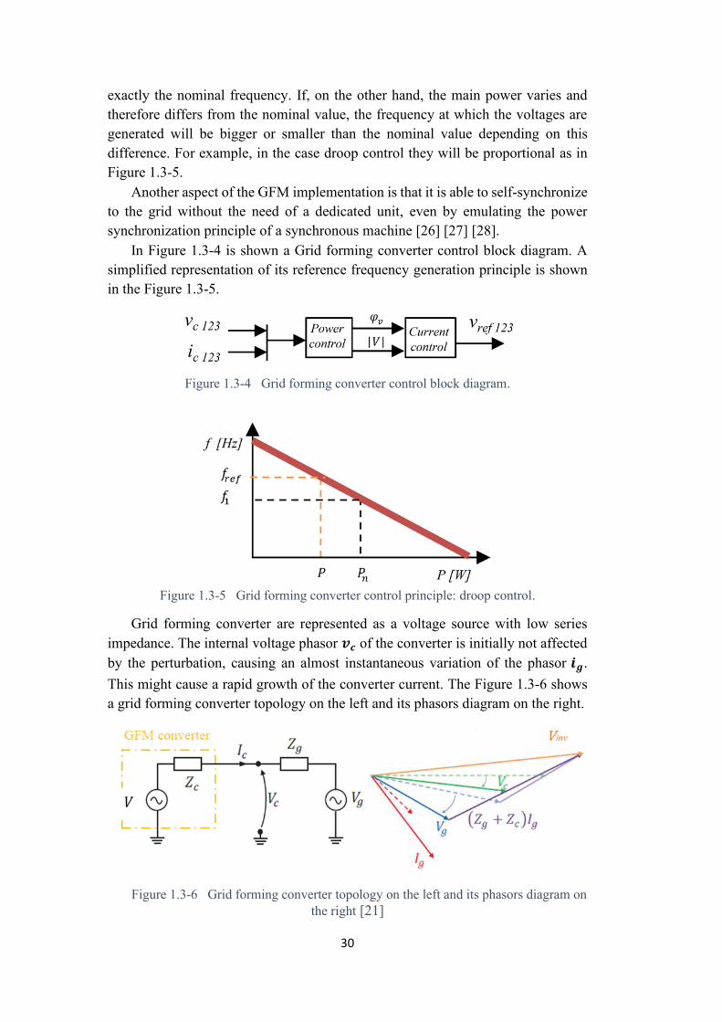
In Figure 13-4 is shown a Grid forming converter control block diagram A simplified representation of its reference frequency generation principle is shown in the Figure 13-5

Figure 13-4 Grid forming converter control block diagram

Figure 13-5 Grid forming converter control principle droop control

Grid forming converter are represented as a voltage source with low series impedance The internal voltage phasor 119959119940 of the converter is initially not affected by the perturbation causing an almost instantaneous variation of the phasor 119946119944 This might cause a rapid growth of the converter current The Figure 13-6 shows a grid forming converter topology on the left and its phasors diagram on the right

Figure 13-6 Grid forming converter topology on the left and its phasors diagram on the right [21]

31

When it is connected to the grid GFM control actively controls the gridrsquos

frequency and the output voltage The rotational speeds of synchronous generators are directly linked to the electrical output frequency causing these generators to act as grid-forming sources

To fully understand how these two types of control work simulations carried out with PLECS software are made where these control strategies have been implemented in a simple and simplified manner The focus is on the converter frequency control which is the main mechanism that makes a converter operating as grid-forming or grid-following

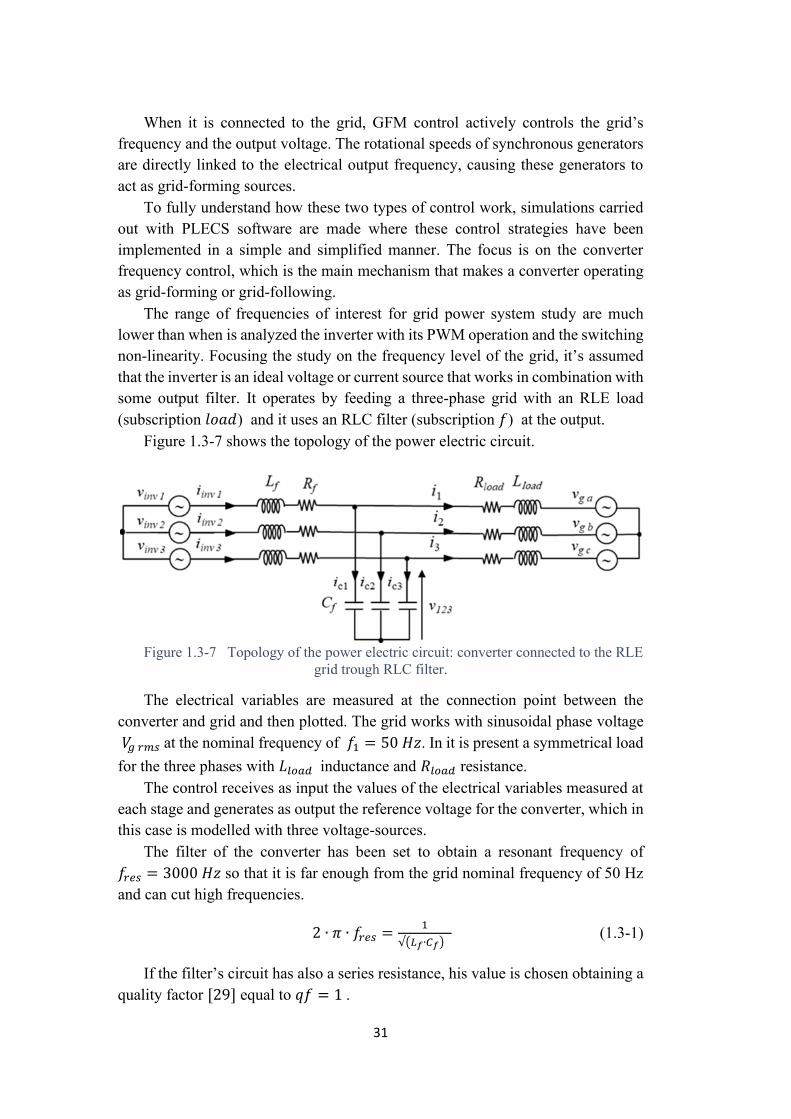
The range of frequencies of interest for grid power system study are much lower than when is analyzed the inverter with its PWM operation and the switching non-linearity Focusing the study on the frequency level of the grid itrsquos assumed that the inverter is an ideal voltage or current source that works in combination with some output filter It operates by feeding a three-phase grid with an RLE load (subscription 119897119900119886119889) and it uses an RLC filter (subscription 119891) at the output

Figure 13-7 shows the topology of the power electric circuit

Figure 13-7 Topology of the power electric circuit converter connected to the RLE

grid trough RLC filter

The electrical variables are measured at the connection point between the converter and grid and then plotted The grid works with sinusoidal phase voltage 119881119892 119903119898119904 at the nominal frequency of 1198911 = 50 119867119911 In it is present a symmetrical load for the three phases with 119871119897119900119886119889 inductance and 119877119897119900119886119889 resistance

The control receives as input the values of the electrical variables measured at each stage and generates as output the reference voltage for the converter which in this case is modelled with three voltage-sources

The filter of the converter has been set to obtain a resonant frequency of 119891119903119890119904 = 3000 119867119911 so that it is far enough from the grid nominal frequency of 50 Hz and can cut high frequencies

2 ∙ 120587 ∙ 119891119903119890119904 =1

radic(119871119891∙119862119891) (13-1)

If the filterrsquos circuit has also a series resistance his value is chosen obtaining a quality factor [29] equal to 119902119891 = 1

32

119902119891 =1119877119891

radic119871119891

119862119891

(13-2)

The values chosen for the simulations are in Table 13-1

119881119892 119903119898119904 [119881]

119877119897119900119886119889 [Ω]

119871119897119900119886119889 [119898119867]

119877119891

[119898Ω] 119871119891

[119898119867] 119862119891

[ 120583119865]

230 10 1 188 28 1

Table 13-1 Values of the grid and filterrsquos parameters used in the simulation

131 Grid following

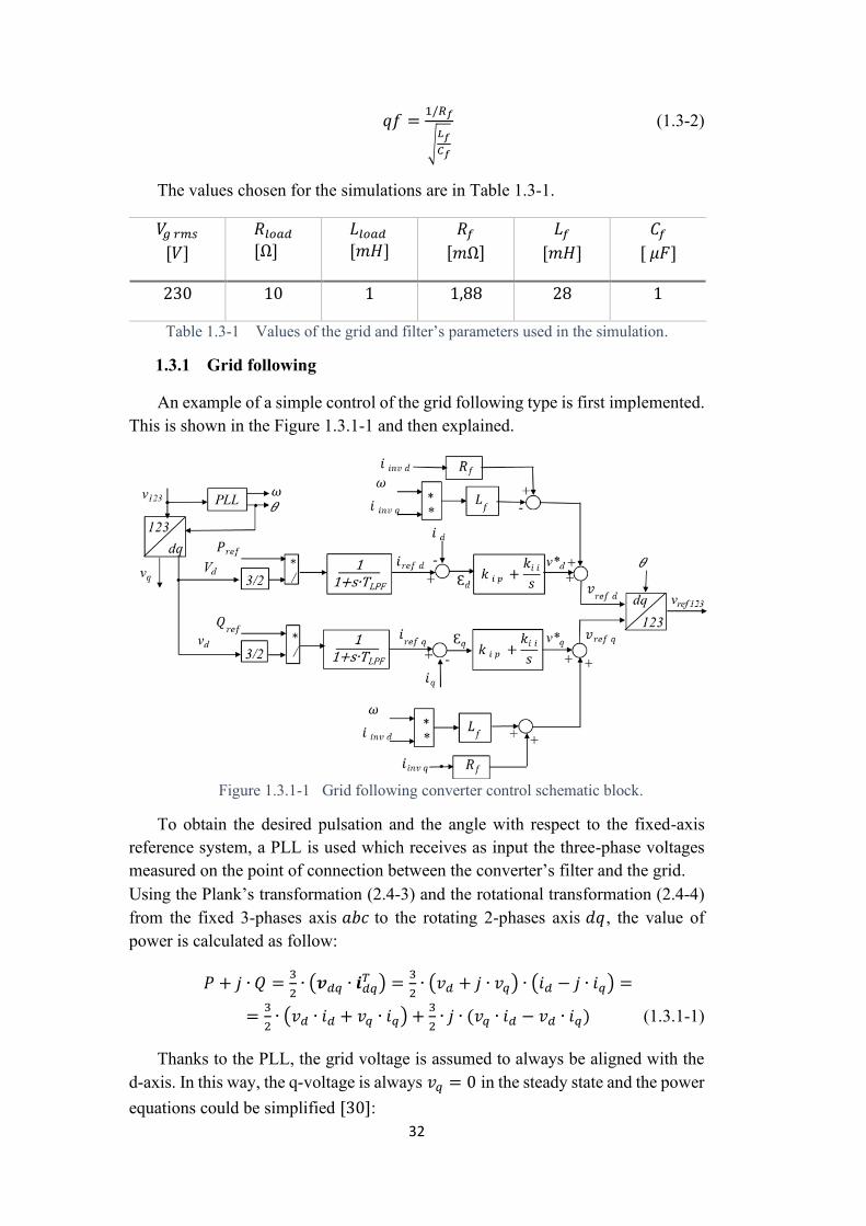
An example of a simple control of the grid following type is first implemented This is shown in the Figure 131-1 and then explained

Figure 131-1 Grid following converter control schematic block

To obtain the desired pulsation and the angle with respect to the fixed-axis reference system a PLL is used which receives as input the three-phase voltages measured on the point of connection between the converterrsquos filter and the grid Using the Plankrsquos transformation (24-3) and the rotational transformation (24-4) from the fixed 3-phases axis 119886119887119888 to the rotating 2-phases axis 119889119902 the value of power is calculated as follow

119875 + 119895 ∙ 119876 =3

2∙ (119959119889119902 ∙ 119946119889119902

119879 ) =3

2∙ (119907119889 + 119895 ∙ 119907119902) ∙ (119894119889 minus 119895 ∙ 119894119902) =

=3

2∙ (119907119889 ∙ 119894119889 + 119907119902 ∙ 119894119902) +

3

2∙ 119895 ∙ (119907119902 ∙ 119894119889 minus 119907119889 ∙ 119894119902) (131-1)

Thanks to the PLL the grid voltage is assumed to always be aligned with the d-axis In this way the q-voltage is always 119907119902 = 0 in the steady state and the power equations could be simplified [30]

33

119875 + 119895 ∙ 119876 =3

2∙ (119959119889119902 ∙ 119946119889119902

119879 ) =3

2∙ (119907119889 ∙ 119894119889) minus

3

2∙ 119895 ∙ (119907119889 ∙ 119894119902) (131-2)

Reversing the equation is possible to obtain the reference currents for the active and reactive power respectably simply dividing the power for the peak grid voltage

119894119903119890119891 119889 =

119875119903119890119891

15∙119907119889

119894119903119890119891 119902 =119876119903119890119891

15∙119907119889

(131-3)

In the schematic block a simple low pass filter LPF is added to eliminate the high frequency noisy and to decouple the power response from the current response It helps the system calculating the error of current In this model a value of 119879119871119875119865 = 01 119904 is used [31]The equation expressing the voltage of the connection point between converter and grid in the steady state is

119959119941119954 = 119877119897119900119886119889 ∙ 119946119941119954 + 119895 ∙ 120596119892 ∙ 119871119897119900119886119889 ∙ 119946119941119954 + 119959119944 119941119954 (131-4)

Using a PI controller that receives as input the current value of 119946119941119954 the reference voltage value 119959119941119954lowast in the point of connection between the filter and the grid is obtained Considering that the voltage on the filter capacitor is equal to the one in input of the grid by measuring the output current of the converter 119946119946119951119959 119954119941 is possible to determine the voltage value to be supplied by the converter

119959119946119951119959 119941119954 = 119877119891 ∙ 119946119946119951119959 119941119954 + 119895 ∙ 120596119892 ∙ 119871119891 ∙ 119946119946119951119959 119941119954 + 119959119941119954 (131-5)

Using the pulsation 120596 in output of the PLL the reference voltage 119959119955119942119943 119941119954 can be calculated as [32]

119959119955119942119943 119941119954 = 119877119891 ∙ 119946119946119951119959 119941119954 + 119895 ∙ ω ∙ 119871119891 ∙ 119946119946119951119959 119941119954 + 119959119941119954lowast (131-6)

In the current loop the PI regulator is used to determinate the reference grid voltage for the d and q axis using gains

119896119894 119901 = 119871119891 ∙ 120596119887119886119899119889119896119894 119894 lt 119896119894 119901 ∙ 120596119887119886119899119889

(131-7)

Values 119896119894 119901 = 6 and 119896119894 119894 =500 has been used As example a simulation has been carried out

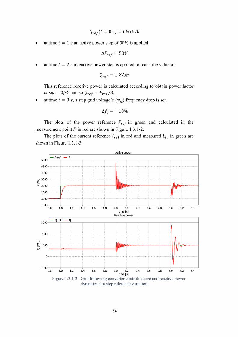
bull the start active and reactive power values are 119875119903119890119891(119905 = 0 119904) = 2 119896119882

34

119876119903119890119891(119905 = 0 119904) = 666 119881119860119903

bull at time 119905 = 1 119904 an active power step of 50 is applied

Δ119875119903119890119891 = 50

bull at time 119905 = 2 119904 a reactive power step is applied to reach the value of

119876119903119890119891 = 1 119896119881119860119903

This reference reactive power is calculated according to obtain power factor 119888119900119904120601 = 095 and so 119876119903119890119891 asymp 1198751199031198901198913

bull at time 119905 = 3 119904 a step grid voltagersquos (119959119944) frequency drop is set

Δ119891119892 = minus10

The plots of the power reference 119875119903119890119891 in green and calculated in the measurement point 119875 in red are shown in Figure 131-2

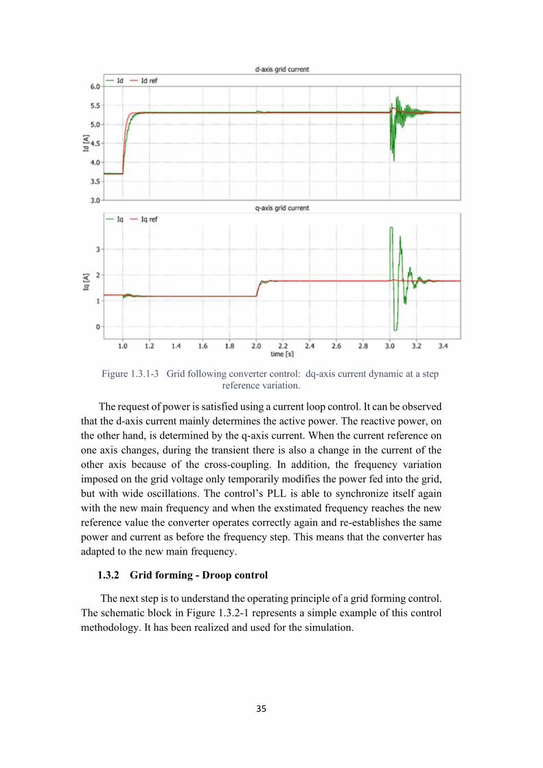
The plots of the current reference 119946119955119942119943 in red and measured 119946119941119954 in green are shown in Figure 131-3

Figure 131-2 Grid following converter control active and reactive power

dynamics at a step reference variation

35

Figure 131-3 Grid following converter control dq-axis current dynamic at a step reference variation

The request of power is satisfied using a current loop control It can be observed that the d-axis current mainly determines the active power The reactive power on the other hand is determined by the q-axis current When the current reference on one axis changes during the transient there is also a change in the current of the other axis because of the cross-coupling In addition the frequency variation imposed on the grid voltage only temporarily modifies the power fed into the grid but with wide oscillations The controlrsquos PLL is able to synchronize itself again with the new main frequency and when the exstimated frequency reaches the new reference value the converter operates correctly again and re-establishes the same power and current as before the frequency step This means that the converter has adapted to the new main frequency

132 Grid forming - Droop control

The next step is to understand the operating principle of a grid forming control The schematic block in Figure 132-1 represents a simple example of this control methodology It has been realized and used for the simulation

36

Figure 132-1 Grid forming converter droop control schematic block

The baseline solution of the GFM control is a frequency regulation of the active power value A proportional droop control gain 119896119889119888 = 0001 is introduced after the calculation of the power deviation obtained from the difference between the nominal and the actual value The current power is calculated through the measurements made in the grid [33] Its value determines how much frequency variation the converter must add compared to the nominal frequency for the voltage reference generation [34] [35]

The power measurements are low pass filtered with cut-off pulsation 120596119871119875119865 before being passed on to droop control This is done because the high oscillations would make the result of the subtraction with a constant value as oscillating as measures Adding the nominal frequency 1198911 and multiplying for 2 ∙ π the pulsation 120596 is obtained Then integrating it the reference angle 120579 is obtained The final function works calculating the modulation index requested for the three phases as sinusoidal phases

119898119894 =1198811198861198981199011198811198631198622

∙ sin [120579 minus (119896 minus 1) ∙ (120587 ∙2

3)] (132-1)

for 119896 = [1 2 3] relative to the three phases Because the high frequency dynamic introduced by PWM modulation is

neglected the reference voltages for every phase 119907119903119890119891 123 is simple obtained multiplying the modulation index for the quantity

119881119863119862

2 119881119886119898119901 = radic2230 119881

It is the amplitude value of the converter reference voltage [36] So the reference voltage is

119907119903119890119891 119896 = 119881119886119898119901 ∙ sin [120579 minus (119896 minus 1) ∙ (120587 ∙2

3)] (132-2)

for 119896 = [1 2 3]relative to the three phases A simulation is performed by using a three-phase resistive-inductive load The

topology of the power electric circuit used in this simulation is in Figure 132-2

37

Figure 132-2 Topology of the power electric circuit used in simulation converter connected to the RL grid trough RLC filter

In the simulation bull an initial reference value for power and frequency has been set

119875119899(119905 = 0) = 156 119896119882

1198911(119905 = 0) = 50 119867119911

bull at time 119905 = 1 119904 the load request step is obtained by halving the value of the load resistance

119877119897119900119886119889prime =

119877119897119900119886119889

2

120549119875119903119890119891 = 50

bull at time 119905 = 2 119904 the nominal powerrsquos value in the summer is modified by doubling it

119875119899 = 2 sdot 156 119896119882

bull at time 119905 = 3 119904 the nominal frequencyrsquos value in the summer is modified by decreasing it of the 10

Δ1198911 = minus10

bull at time 119905 = 4 119904 the reference voltage amplitude is decreased by the 10

Δ119881119886119898119901 = minus10

The plots of the power and of the frequency are reported in Figure 132-3 where reference values 119875119899 and 1198911 are represented in green and the instantaneous performed values 119875 and 119891 are represented in red

38

Figure 132-3 Grid forming converter control active power and frequency dynamic at step load request reference power frequency reference and voltage drop

variations

Initially since the power on the grid is the same as the reference power 119875 =119875119899 the present frequency is also the same as the reference frequency 119891 = 119891119899 When the load power changes the control reacts by changing the frequency at which the reference voltage is generated The frequency variation applied is proportional to the power variation and it is calculated as dinstance from the reference values set equal to the nomial ones

This is also evident in the waveforms of the voltage and of the current measured on the grid below reported in Figure 132-4 When the power and frequencyrsquos

reference values 119875119899 and 1198911 of the control are changed the droop-control line of the frequency-power graph represented in Figure 132-3 is shifted causing the converter to operate at a new operating point The effects on the current power and frequency are of different magnitude because of the droop-gain value The voltage drop creates a reduction in the main power and so the converter reacts by returning higher frequency waveforms

The voltage and current measurements are shown in Figure 132-4

39

Figure 132-4 Grid forming converter control phase voltage and current dynamic at step load request reference power frequency reference and voltage drop

variations

The ultimate expression of grid-forming control is inspired by the virtual emulation of the dynamics and control of a synchronous alternator The general idea is to control the converter signals to behave like a synchronous machine This emulation of the synchronous machine transforms the converter into a virtual synchronous machine using an algebraic model of a synchronous machine where there is an analogy between the converterrsquos terminals voltage and the generatorrsquos stator voltages

14 The Virtual Synchronous Machine control

As required by grid codes the power balance between the power generation and the power demand following a frequency variation event must be reached in a fast enough way such that the frequency excursions remain close to the reference frequency of 50 Hz or 60 Hz

As it has just been seen in the Chapter 11 during a load power variation event a frequency drop is also generated The primary control must arrest the fast frequency decline its nadir in the timescale of seconds and then the secondary frequency regulation restores the frequency in some minutes

When the frequency drops synchronous generators autonomously turn slower and reduce the kinetic energy stored in their rotors and deliver a kinetic power thus

40

helping the system to mitigate the frequency drop and to eliminate the frequency deviation restoring the nominal value [37]

As the penetration level of renewable energy sources grows inertia decreases The effect of the primary control is contributed by both frequency drop and inertia but inertia is an inherent property of synchronous generators and not of static converter For this reason is mandatory to give to this technology the inertia sensibility This could be done implementing an algorithm that works elaborating a power variation reference equal to the mechanical power that an equivalent synchronous machine would deliver

A method by which a converter can be controlled to mimic the behavior of a synchronous machine is the Virtual Synchronous Machine control The equations used in it are the same used for the frequency regulation made with alternators including the swing equation (11-1) that introduces the dynamic of the regulation and the link between the powerrsquos difference and the frequencyrsquos variation If a

converter that uses this kind of control is connected to the grid no difference would be felt from the grid side

Disadvantage of the use of a VSM control is that as a synchronous machine a loss of stability due to under excitation or load-angle too big could occur Advantage over the introduction of inertia in the system is that itrsquos possible to

choose the parameters such as inertia droop coefficients and so on [38] [39] [40] [16]

To understand how to regulate the frequency using a converter and introducing also the typical dynamics of regulation using synchronous alternators the dynamic model of the frequency regulation made with synchronous generators is merged into the Grid Forming control The grid configuration the control structure and the turbine simulation parameters remain the same previously used

The block schematic of the implemented control is shown in Figure 14-1 It shows the Virtual Synchronous Machine control block diagram realised for the simulation

bull the part coming from a typical GFM control is highlighted in orange bull the part that simulates the behaviour of the synchronous machines in

frequency regulation using pu values is highlighted in green

41

Figure 14-1 Grid forming converter Virtual Synchronous Machine control

schematic block in orange the part coming from a typical GFM control in green the part that simulates the synchronous machine frequency regulations behavior

After calculating the load power variation from the nomial value the signal is sent as input to the block that simulates the closed-loop frequency regulation done with synchronous generators It returns the frequency variation from which once the reference frequency value is known the instantaneous frequency and the electrical angle that the regulator must apply to the voltage reference are calculated The converter then feeds the grid generating the desired three-phase voltage at the same frequency and with the same dynamics that the simulated machine would have if a real and identical one has been placed in its place In this way the new load power demand is satisfied

A simulation is carried out where using a resistive-inductive grid a 10 increase in load power is required at time 119905 = 10 119904 by decreasing the load resistance 119877119897119900119886119889 value by 10

Because it is intended to emulate the same dynamics as in the example given in Chapter 11 the same values for the control parameters (Table 14-1) have been used in the block of the emulated inertia dynamic

Figure 14-2 shows the plots of the phase grid current near the power steprsquos

time

Figure 14-2 Grid Forming Virtual Synchronous Machine converter control phase current dynamic at step load request

42

Figure 14-3 shows the power and frequency calculated by the measures on the grid

Figure 14-3 Grid Forming Virtual Synchronous Machine converter control

power and frequency dynamics at step load request

Figure 14-4 shows the frequency and power deviations calculated by the emulation block of the synchronous machines system

All the plots are below commented

43

Figure 14-4 Grid Forming Virtual Synchronous Machine converter control dynamic of the power and frequency responses of the simulated machines system

-dynamic response at step load request

As can be seen from the figures the power variation is realized by an increase in the amplitude of the current flowing in the grid as a result of a step reduction in the load equivalent resistance 119877119897119900119886119889 At the demand for more power requested by the load the turbine simulation block calculates how much the frequency change should be calculating it as if the virtual turbine is connected with droops 119887119879 119887119875 and time constants 119879119886 of the allocated controllers The simulated mechanical power variation Δ119875119898 is used to calculate the virtual inertia power Δ119875119882 and then using the system inertia value of the virtual machine 119869 the speed variation Δ119891 that this machine would have in that situation is obtained The converter generates voltage at the calculated frequency and imposes it on the grid which will have AC voltages and currents at the same frequency as the converter

In fact the frequency plots show that the main frequency in Figure 14-3 has the same waveform as that simulated by the virtual machine control in Figure 14-4 This is what distinguishes the virtual synchronous machine GFM control from others

More significantly the graph in Figure 14-4 showing the dynamics of the power variation of the emulated synchronous generators in green (with primary and secondary regulation respectively in red e yellow) actually follows the one of the measured power on the grid in Figure 14-3 This demostrates that the converter manages to behave exactly as if in its place there is a frequency regulation system

44

with synchronous machines equal to those emulated and that the grid does not feel any difference due to the use of the converter as a power source This validates the use of the control

45

2 Average model of string inverters

21 Motivation

TRUST-PV is a project created to increase the performance and reliability of PV components and PV systems in large distributed andor utility-scale PV areas

In the framework of the PV TRUST project activities it has been proposed to carry out with Enel a system study involving a detailed power system with increasing levels of PV penetration using different strategies such as grid following grid forming and a mixture of them to assess the grid support and ancillary services that the power plant controllers and inverters can provide To do this task has been asked to start a joint activity in which Huawei would provide a generic but detailed model Huawei agreed to plan the joint activity from the inverter level to the power system solution [41] [42]

As Huaweis strengths are in inverter controls the company aimed to design control strategies possibly based on existing techniques to evaluate grid-following strategies with grid support and grid-forming strategies eg by introducing virtual inertia to be tested in a large grid system Above all one of Huaweis main interests in PV h2020 Trust is to show virtual inertia capabilities for frequency regulation leaving some margin in dispatching or transient overload to IGBTs and also oversizing DC capacitors

Enel on the other hand proposed to build it and integrate it into an existing electrical system They will additionally contribute with power system studies and detailed modelling for all components to be included in the simulation [43]

At the end of the poject the results would be evaluated by both companies together

22 Averaging versus switching models

Switching or avarage model are two different approaches to represent the behaviour of the system under observation Both the two models are able to represent the functionality of the controller in the same way From the viewpoint of the power stage the only difference between them is that the switching model uses the detailed three-phase component of the inverters power electronics device to emulate its behaviour whereas the average model uses three signal-controlled voltage sources

Depending on the task the type of device or controller under test and the computing power available the choice can fall on one model or the other

46

If it is intended to realise the control of the inverter itself the switching dynamics must also be analysed and so a switching model is preferable However a higher resolution is required

On the other hand if it is desired to develop controllers for grid studies and to investigate energy resources it is preferable to use models for inverters using average values since that is the level at which the power transfer between the connected devices takes place For this reason highly detailed switching models are generally not necessary for that application [44]

By focusing more on the response of the electrical system rather than the behavior of the converter generic models are provided that well could represent the dynamics of the control loops under relevant conditions [45]

Moreover the collaboration of more than one company implies finding solutions that are good for both In fact the collaborating company deals more with studies related to grid transmission distribution generation industrial plants which are at slow dynamic and they neglect high frequency dynamic effects such as discontinuities introduced by the converterrsquos modulation technique or the delays introduced by the converters in use for sampling the useful variables for the control In fact it is used to make simulations with software such as DIgSILENT

Overall this case study requires to work with models at average values By doing so the level of detail of the inverter control goes up to the current control The main focus remains on the AC part of the grid that is composed by power loops (activereactive) inertial emulation loops internal current loops The action of the current loop control returns a voltage reference or a modulation signal to convert the DC-link voltage and that injects a dependent three-phase voltage as a source in the AC side of the power system model After this voltage source an LCL filter must be inserted and the current control loop must consider its presence Assuming proper sizing of the LCL filter it is permissible to neglect high frequency phenomena since they do not modify the response of the power transfer between the grid and the connected devices In simulations of mass power systems with PV converterrsquos DC dynamic is not considered unless there is a sudden change in irradiation reaching the PV panels For these reasons the DC-link voltage control placed between the converter and the PV source is structured to be sensitive to variations in power generation

In this regard it has been chosen to realize an avarege model using the simulation program PLECS that can be easily adapted to other tools

23 Lumped model of a string

When setting up a photovoltaic system it must be ensured that the output voltage and current are at the required levels This determines the configuration of the circuit and the connection of the photovoltaic panels to each other The first way to connect the panels together is in series until the desired voltage is reached An example of string PV is in Figure 23-1

47

Figure 23-1 String PV obtained connecting several PV panel in series

Proceeding in a similar way in order to obtain more power than the one that a single string of panels in series can provide several strings with the same number of PV panels are connected each other in parallel forming a PV module [46] as shown in Figure 23-2 They forms a PV module

Figure 23-2 Parallel of more string PV Output current and voltage are managed by

a converter

This is also what is to realize in the companys project In fact it is planned to

use string PV panels connected to an inverter that manages them to work at stable power levels

Then more inverters are connected together to deliver a higher power level The interconnected converter complex acts as a bridge between the energy

48

production of the photovoltaic panels and the grid Each converter is connected to the grid through an LCL filter whose task is to reduce current ripple on the line

The representation of the AC power system of an inverter connected to the grid is shown in Figure 23-3

Figure 23-3 Electrical circuit of the power system formed by a converter connected

to the grid trough a LCL filter

The converter used is a voltage source converter (VSC) In the Figure 23-3 the voltages 119959119944 119938119939119940 119959119940 120783120784120785 and 119959119946119951119959 120783120784120785 represent the solid

grid the voltage in the point of connection and the VSCrsquos voltages respectively The LCL output filter is formed by the converter side inductive filter the capacitance and transformer leakage inductance

The inductive filter in the converterrsquos side is defined by the series inductance 1198711198911 and resistance 119877119891 1198711198912 is the output inductance of the filter but in the calculation it can be neglected because of its small value respected to other variables The capacitance is given by a parallel capacitance 119862119891 in series with a small equivalent series resistor 119877119888

The transformer model is given by a leakage inductance 119871120590 and an equivalent winding resistor 119877120590 in series

The grid impedance is represented by 119885119892 which depends on power system circuit and grid conditions

Converter control commonly consists of an outer DC-link voltage control loop and an inner current control loop For some applications with line current feedback the well-known PI controller in the synchronous reference 119889119902 frame can be employed However the inner PI-based current control is not suitable for many applications depending on the ratio of LCL resonance frequency to control frequency

The VSC is an active component Due to its discrete operation and PWM modulation technique the effectiveness of the control is increasingly reduced as the frequency increases because system delays and non-linear effects tend to compromise its passivity property However these effects can be minimized by including the LCL filter as part of an external VSC admittance This hypothesis is supported by the fact that at high frequencies the disturbances generated at the

49

connection point are absorbed by the LCL capacitor branch and therefore are not able to create positive feedback in the VSC

The LCL resonant pulsation is [47]

120596119903119890119904 = radic1198711198911+119871120590

1198711198911∙119871120590∙119862119891 (23-1)

The selection of 120596119903119890119904 involves a trade-off between control interactions and filtering At low values of the ratio of LCL resonance frequency to control frequency the feedback of the converterrsquos PI current control can lead to instability For these applications active resonance damping gets integrated into the current control loop Typically the control action calculation also includes an 119959119914 voltage feedforward 119959119943119943 double path with the objectives of provide a filtered value of the main grid component to improve the initial transient and an active damping action based on capacitor voltage derivative term

Design for passivity is approached as a reliable method to assure the stability of LCL grid-connected VSC working in power systems with potential resonances Its frequency region for design is reconsidered by having into account non-linear ZOH and PWM effects and the nature of the LCL filter topology

This proposed method models the converter control and the LCL filter as an equivalent admittance 119884119888 The rest of the grid is modelled as an equivalent impedance 1198850119892 The stability condition is given by the fact that considering 1198850119892 to be formed by passive elements only the whole system formed by 119884119888 1198850119892 is stable if 119884119888 is also passive In practice design for passivity aims to define converter control actions that shape 119884119888 to be passive in a specified range of frequencies

Considering the LCL grid-connected VSC the outer admittance 119884119888 sets the dynamics by its interactions with 119885119892

The outer admittance is given by

119884119892 = (119895120596 ∙ 119862119891 + 119884119888)1

119895120596∙119871120590 (23-2)

The term 119895120596 ∙ 119862119891 + 119884119862 is the inner admittance and has been defined as the parallel of the converter admittance 119884119888 and the filter capacitor branch considering null the series resistance Only 119884119888 models the converter control actions but the remaining 119884119892 components are passive As the capacitive branch admittance increases with frequency the assumption |119895120596 ∙ 119862119888| ≫ |119884119888| becomes reasonable at frequencies above 120596119903119890119904 At high frequency the capacitor branch becomes dominant and mainly sets the admittance seen by 119959119914 120783120784120785 to the voltage source converter Having stability means that the high frequency components in the main side flow principally through the capacitor branch and they go hardly into the voltage source current path of the converter In this way the consequences on the control resulting from the disturbance are minimal and not sufficient to cause positive feedback or instability To satisfy this assumption |119884119888| should be small at high frequencies which is achieved by the passivity method

50

A second issue that arises comes from the digital sampling for measurements of electrical quantities useful for the control The function in the frequency domain that describes the practical signal reconstruction done by a conventional digital-to-analog converter (DAC) is the Zero Order Hold (ZOH) [48]

119885119874119867(120596) =1minus119890minus119895120596∙119879119904

119895120596∙119879119904 (23-3)

Its frequency response is non-linear and aliasing occurs at frequencies higher than half of the main frequency Itrsquos shown in the Figure 23-4 The aliasing area is highlighted in yellow

Figure 23-4 ZOH frequency response The yellow zone corresponds to alias region

[49]

Anti-aliasing filters are designed so that the frequencies close to 1205961199042 are well attenuated which implies a high order analogue filter with a cut-off frequency well below 1205961199042 The filter is a low-pass filter and it adds a significant phase delay in the closed loop and so it can compromises the stability properties For this reason the frequency region in which anti-aliasing is effective should be outside the working range of the control

Another problem of non-linearity is given by PWM operation because it generates voltage harmonics at multiple frequencies They are dependent on the fundamental component amplitude and angle and the carrier phase angle

The internal admittance of the VSC can be modelled by a reduced-order filter in the Z-domain which depends mainly on the proportional damping and active (controller) gains

To create a passivity model with admittance expressions for the converter 119884119888 and for the grid 119884119892 it is taken into account that the non-linearities of the ZOH and the PWM operation depend on the references of the fundamental components Therefore these non-linearities can behave as a disturbance in the frequency region for the design

It is also assumed that bull the reference current of the controller is zero in the range of frequencies at

which a passive behaviour of the current controller is wanted (ie above the theoretical closed loop bandwidth)

bull the analytical expression of 119884119888 is calculated by an 119959119940 impulse responses considering it linear in the design region

51

bull the effect of anti-aliasing filters is negligible in the design region Under these assumptions the admittance of the converter in the Z-domain is

described by a third-order expression with zeros and poles depending on the active damping gain 119896119886119889 and the proportional gain 119896119901 respectively of the controller [49]

119884119888(119911) =119894119888

119907119862=

05∙1199113+05∙1199112minus119896119886119889119879119904∙119911+

119896119886119889119879119904

119911∙(1198711198911119879119904∙1199112minus

1198711198911119879119904∙119911+119896119901)

(23-4)

A convenient combination of 119896119886119889 and 119896119901 provides a stable polezero cancellation which reduces the 119884119888(119911) order to a first one

The polo-zero cancellation is obtained by choosing for the control gains equal to [50]

119896119886119889 =

2

3∙ 119879119904

119896119901 =2

3∙1198711198911

119879119904

(23-5)

The admittance of the converter is simplified by becoming first-order

119884119888(119911) =119879119904

2∙1198711198911∙ 119911+2

119911 (23-6)

In this way the passivity of the converters admittance is obtained The expression obtained has a zero in 119911 = minus2 which creates a delay that is greater when the frequency is high Additionally despite being a first-order expression the phase delay reaches minus180deg at the Nyquist frequency

According to have a frequency response it is possible to turn 119884119888(119911) into 119884119888(120596) simply calculating 119884119888(120596) = 119884119888(119911 = 119890119895120596119879119904)

For the project that itrsquos wanted to be realized the control of a single converter

is not sufficient Given the need to manage a higher power level than a single converter would be able to do it is necessary to connect several identical converters in parallel This creates a String Inverter Model [51] as represented in the Figure 23-5

52

Figure 23-5 String inverter obtained connecting N inverter in parallel

Thus the problem of having to make an analysis of the overall system arises Simulations should consider the behavior and control of each individual inverter The level of detail of the system and the computational power required become enormous For this reason a lumped model must be used that is able to represent the behavior of several voltage source inverters connected in parallel through LCL filters to the grid The advantage of this model is to reduce the order of the system but because of this information about individual converters are lost and it is not possible to observe what is happening in one of them

The aim is to use the equations that govern each individual converter and manipulate them to derive equivalent ones reduced in number capable of representing the response that would be obtained if a single converter is used instead of them but with a power output equivalent to that delivered by the converters in parallel

Considering a generic 119899 LCL filter between the 119873119894119899119907 converters connected in parallel it is formed by a primary and secondary side which will be connected to the converter and the grid respectively It is represented in Figure 23-6 where

bull 1198711119899 1198712119899 are the inductences of the primary and secondary side bull 119862119899 is the filterrsquos capacitance bull 119946120783119951 = 119946119946119951119959 119951 and 119946120784119951 = 119946119951 are the currents of the primary and secondary side

of the filter bull 119959119927119914119914 is the voltage at the point of connection bull 119959119862119899 is the voltage on the filter capacitance bull 119959119894119899119907 119899 is the voltage supplied by the converter

53

Figure 23-6 A generic 119899 LCL filter between the 119873119894119899119907 inverter ant the point of

connection PCC

The control equations for the state variables of a generic 119899 converter among the 119873119894119899119907 connected in parallel are [52]

119886)

119889

1198891199051199461119899 = minus

119959119914119951

1198711119899+119959119946119951119959 119951

1198711119899

119887)119889

1198891199051199462119899 =

119959119914119951

1198712119899minus119959119927119914119914

1198712119899

119888)119889

119889119905119959119862119899 =

119946120783119951

119862119899minus119946120784119951

119862119899

(23-7)

To these must be added the equation that interconnects the converter complex with the grid Let 119871119892 119946119892 119959119892 be the total inductance the current and voltage on the grid Resistances are neglected

In Figure 23-7 is shown the point of connection of the 119873119894119899119907 inverters composing the string inverter

Figure 23-7 Point of connection of the 119873119894119899119907 inverters composing the string

inverter

119889) 119889

119889119905119946119892 = minus

119959119944119871119892+ 119959119927119914119914

119871119892

119946119892 =sum 1199462119899119873119894119899119907119899=1

(23-8)

Because of all the converters are equal and they are connected to the same grid via identical LCL filters it is assumed that all inductances and capacitances seen by every individual converter are equal

54

1198711119899 = 11987111198712119899 = 1198712119862119899 = 119862

(23-9)

for every 119899119905ℎ inverter between 119873119894119899119907 Moving from the time domain to the frequency domain and so using Laplace

equations the derivative function 119889119889119905

is replaced by the 119904 complex variable Considering the equations b) (23-7) valid for every inverter they are summed

up for all 119873119894119899119907 converters The resulting equations is

119887) 119904 ∙ 119946119892 = 119904 ∙ sum 1199462119899119873119894119899119907 119899=1 =

1

1198712∙ sum (119959119862119899 minus 119959119875119862119862)

119873119899=1 =

=1

1198712∙ sum (119959119862119899)

119873119894119899119907 119899=1 minus

119873119894119899119907

1198712∙ 119959119875119862119862 (23-10)

As lumped modelrsquos assumptions are considered the average value for the voltage of the capacitance 119959119888 and for current in the inductor 1199461

119959119888 =

1

119873∙ sum (119959119862119899)

119873119894119899119907 119899=1

1199461 =1

119873∙ sum (1199461119899)

119873119894119899119907 119899=1

(23-11)

Thus equation b) of the equivalent aggregate converter is

119887) 119904 ∙ 119946119892 =119873

1198712∙ (119959c minus 119959119875119862119862) (23-12)

So it is possible to obtain the value of 119959119875119862119862

119959119875119862119862 = 119959c minus 119904∙119946119892119873

1198712

(23-13)

Substituting 119959119875119862119862 (23-13) into equation d) (23-12) it is obtained the first equation B) (23-12) that describes the full system

119861) 119904 ∙ 119946119892 = minus119959119944

119871119892+

1

119871119892∙ (119959c minus

119904∙1199461198921198731198941198991199071198712

) =119959119836minus119959119944

119871119892+1198712119873119894119899119907

(23-14)

The second global equation comes from a) (23-7) and it is influenced by the type of control that the converter uses Let there be a generic control function with terms for the voltages of the capacitances and currents passing through the filter inductor

119959119946119951119959 119951 = 119870119881 ∙ 119959119914119951 + 119870119868 ∙ 119946120783119951 + 119870119865 ∙ 119865119899(119904) (23-15)

Equations a) (23-7) becomes

119886) 119904 ∙ 1199461119899 =1

1198711119899∙ ((1 minus 119870119881) ∙ 119959119862119899 + 119870119868 ∙ 1199461119899 + 119870119865 ∙ 119865119899) (23-16)

55

Summing for all the 119873119894119899119907 converter and using the lumped model hypothesis before expressed in (23-9) itrsquos obtained

119904 ∙ sum 1199461119899119873119894119899119907119899=1 =

1

1198711119899∙ ((1 minus 119870119881) ∙ sum 119959119862119899

119873119894119899119907119899=1 + 119870119868 ∙ sum 1199461119899

119873119899=1 +119870119865 ∙ sum 119865119899

119873119894119899119907119899=1

119860) 119904 ∙ 119946120783 =1

1198711∙ ((1 minus 119870119881) ∙ 119959119914 + 119870119868 ∙ 119946120783 + 119870119865 ∙ 119865) (23-17)

The last equation is obtained simply by using the lumped model assumptions (23-9) and summing up the equations c) (23-7) for all the 119873119894119899119907 converters

119904 ∙ sum 119959119862119899119873119899=1 =

1

119862∙ sum (1199461119899 minus

119873

119899=11199462119899)

119862) 119904 ∙ 119959119862 =1

119862∙ (1199461 minus

119946119944

119873) (23-18)

119959119862 1199461 1199462 are the state variables Other variables are inputs except 119865119899 that depends on the control

The obtained ABC equations are valid for a lumped model of a string converter with a generic control strategy

The control for passivity before explained and used in the current loop of the developed control has

119959119894119899119907 119899 = 119896119886119889 ∙ 119904 ∙ 119959119862119899 + 119896119875 ∙ (1199461119899 119903119890119891 minus 1199461119899) (23-19)

Finally substituting (23-19) in the ABC equations the equations of the lumped model of the string converter with the control strategy used in this work are obtained

119860) 119904 ∙ 1199461 =

1

1198711119899∙ 119959119862 +

1

1198711119899∙ (minus119896119901 +

119896119886119889

119862) ∙ 1199461 minus (

119896119886119889

119873119894119899119907∙1198711119899∙119862) ∙ 119946119892 +

119896119901

1198711119899∙ 1199461 119903119890119891

119861) 119904 ∙ 119946119892 =1

119871119892+1198712119873119894119899119907

∙ 119959c minus1

119871119892+1198712119873119894119899119907

∙ 119959119892

119862) 119904 ∙ 119959119862 =1

119862∙ 1199461 minus

1

119862∙119873119894119899119907∙ 119946119892

(23-20)

24 Current control

The AC system operating in three phases is composed of a string converter LCL filters and a connection with the grid trough a step-up transformer Itrsquos

considered a nominal power of the grid equal to 119875119899 = 2 119872119882 The Figure 24-1 represents the power arrangement

56

Figure 24-1 Power arrangement PV generation for N inverters composing a string

LCL filers between inverters and point of connection transformer to connect with the grid

The string converter is considered an aggregated model of 119873119894119899119907 = 20 inverters Each inverter has bull nominal power 119875119899 = 100119896119882 bull output filter lsquos capacitance 119862119891 = 10 120583119865 bull filterrsquos inductances 1198711198911 = 300 120583119867and 1198711198912 = 10 120583119867 Because of the parallel connection the equivalent inductance is simplified with

an LC equal to

119862119891119905119900119905 = 119862119891 ∙ 119873119894119899119907 = 200 120583119865

1198711198911119905119900119905 = 1198711198911119873119894119899119907 = 15 120583119867

The effect of 1198711198912 inductances can be neglected The primary side of the transformer is connected to the output of the converter

working at the nominal voltage of 119881119899 = 460 119881 It is considered a short circuit complex power equal to 119873119904119888 = 20 times the nominal one

119878119904119888 = 119873119904119888 ∙ 119875119899 = 20 ∙ 2 ∙ 106 = 40 119872119881119860

The short circuit impedance is obtained [54]

119885119904119888 =1198811198992

119878119904119888= 53 119898Ω (24-1)

Supposing that the short circuit impedance is only an inductance the short circuit inductance of the transformer is

119871120590 =119885119904119888

2 ∙120587 ∙119891119899= 1683 120583119867 (24-2)

This value is very similar to that of the filter

57

To implement a control algorithm the output voltage 119959120783120784120785 and current 119946119946119951119959 120783120784120785 of the converter and currents on the grid 119946119938119939119940 are measured The Figure 24-2 represents the equivalent electric circuit of the system described above

Figure 24-2 Equivalent AC system arrangement

The presented control works in the two-phase 119889119902 reference system rotating at the grid frequency For this reason the measured quantities are transformed using Parke transformations from the three-phase frame 119886119887119888 or 123 to the 1205721205730 orthogonal frame

119879123rarr1205721205730 =2

3sdot [

1 minus12 minus12

0 radic32 minusradic3212 12 12

] (24-3)

In the transformation the coefficient is used to have a transformation that maintains invariant the vectorrsquos amplitude Because of the star connection the unidirectional component resulting from the 0 sequence is considered null

The rotational transformation rotates the spatial vector described by the fixed axes 120572120573 of the angle 120579 to the 119889119902 rotating reference frame

119877(120579)120572120573rarr119889119902 = [cos (120579) minussin (120579)sin (120579) cos (120579)

] (24-4)

To determine the angle of rotation 120579 a Phase locked loop (PLL) is used which receives as input the measured three-phase voltage 119959120783120784120785 In this way it is possible to work in the 119889119902 reference frame

The three-phase AC circuit is described by the following equations

119889

119889119905119946119946119951119959 120783120784120785 =

1

1198711198911119905119900119905∙ (119959119842119847119855 120783120784120785 minus 119959120783120784120785) (24-5)

119889

119889119905119959120783120784120785 =

1

119862119891119905119900119905∙ (119946119946119951119959 minus 119946119938119939119940) (24-6)

119889

119889119905119946119938119939119940 =

1

119871120590∙ (119959120783120784120785 minus 119942119938119939119940) (24-7)

By applying the transformations the equations that describe the system in the frequency domain are expressed as follow where

58

bull 119895 represents the complex variable bull 120596 represents the pulsation

They are the cause of the cross-coupling terms resulting from the rotational transformation

The dynamic of the converterrsquos output current in the 119889119902 frame is described by the equation

119904 ∙ 119946119946119951119959 119941119954 =1

1198711198911119905119900119905∙ (119959119946119951119959 119941119954 minus 119959119941119954) + 119895120596 ∙ 119946119946119951119959 119941119954 (24-8)

In the steady state the Laplace variable tends to zero and the pulsation is equal to the nominal value

119904 rarr 0

120596 rarr 2 sdot 120587 sdot 1198911

The converterrsquos output voltage is

119959119946119951119959 119941119954 = 119959119941119954 minus 119895 ∙ (2 sdot 120587 sdot 1198911) ∙ 119946119946119951119959 119941119954 ∙ 1198711198911119905119900119905 (24-9)

Replacing the voltage 119959119941119954 with the constitutive capacitance equation and so with the integral of its regime equation

119959119941119954 =1

119904∙119862119891119905119900119905∙ (119946119946119951119959 119941119954 minus 119946119941119954) (24-10)

the final equation for the reference volteges of the current loop is obteined

119959119946119951119959 119941119954 =1

119904∙119862119891119905119900119905∙ (119946119946119951119959 119941119954 minus 119946119941119954) minus 119895 ∙ 21205871198911 ∙ 119946119946119951119959 119941119954 ∙ 1198711198911119905119900119905 (24-11)

To have a single input ndash single output (SISO) system also eliminating the additive disturbance it is obtained the matrix 119866(119904)

119866(119904) = 119946119946119951119959 119941119954(119904)119959119941119954(119904) =1

1198711198911119905119900119905∙119904∙ [1 00 1

] (24-12)

A proportiona integral (PI) controller is used to obtain the voltage reference from the error between the reference current and the measured one at the output of the inverter

119870119894(119904) = 119896119901119894 +119896119894119894119904=

119904sdot119896119901119894+119896119894119894

119904= 119896119901119894 sdot

119904+119896119894119894119896119901119894

119904= 119896119901119894 sdot

119904+120596119911

119904 (24-13)

A medium time delay 120591119889 = 15119891119904 due to the discrete-time operation is considered 119891119904 represents the frequency of samplings In the case under

59

consideration itrsquos value is 119891119904 = 2 ∙ 18 119896119867119911 The Laplace function with added the effects of the delay is [55]

ℒ(119891(119905 minus 120591119889)) = ℒ(119891(119905)) ∙ 119867119889(119904) = ℒ(119891(119905)) ∙1minus

1205911198892∙119904

1+1205911198892∙119904

(24-14)

The cascade of all transfer functions gives the current open loop transfer function

119867119900119897119894(119904) = 119870119894(119904) ∙ 119867119889(119904) ∙ 119866(119904) (24-15)

A damping value bigger than 120577 ge 05 is mandatory to ensure negative feedback and system stability The proportional gain 119896119901119894 determines the crossover frequency and the bandwidth of the current regulator This must be smaller than the converterrsquos bandwidth that is set at 119901119888119900119899119907 = minus1120591119889 To have 119867119900119897119894(119904) calculated at the crossover pulsation 120596119888 with a Bode plot that falls with a slop of minus20 119889119887 for frequency decade guarantees the stability and a phase margin 119901119898 ge 45deg

119867119900119897119894(119904 rarr 119895 sdot 120596119888) =119896119901119894

119895sdot120596119888∙ 1 ∙

1

1198711198911119905119900119905= 1

Choosing the crossover pulsation equal to

120596119888 =1

120591119889=

119891119904

15

and so working with critical damping 120577 = 05 and 119901119898 = 45deg the proportional gain is set as

119896119901119894 =119891119904

15∙ 1198711198911119905119900119905 (24-16)

Subsequently the regulatorrsquos integrator gain must be set having into account the design rule

119896119894119894 ge 2 ∙ 119896119901119894 ∙ 1205961 (24-17)

where 1205961 is the fundamental frequency

In closed loop the zero of the regulator 120596119911 =119896119894119894119896119901119894

of the equation (24-13)

attracts the closed loop poles to the right half plane of the complex-plane The gain has to move the main zeros of the PI controller as far as possible from the right half-plane by identifying the critically For this reason it is chosen a value of [34]

119896119894119894 = 2 ∙ 119896119901119894∙ 1205961 (24-18)

Using the expressed data the gains have the values of

119896119901119894 = 0384

60

119896119894119894 = 241

A 119959119941119954 voltage feedforward is added to provide a filtered value of the main grid component to improve the initial transient and an active damping action 119896119886119889 based on capacitor voltage derivative term To make this feedforward should be added the value

119959119943119943 119941119954(119904) = 119904 ∙ 119896119886119889 ∙ 119959119941119954 (24-19)

To avoid the introduction of a derivative term in the system it is preferable to replace 119959119941119954 as done in the equation (24-10)

119959119941119954 =1

119904∙119862119891119905119900119905∙ (119946119946119951119959 119941119954 minus 119946119941119954)

In this way the additional feedforward term is

119959119943119943 119941119954(119904) = 119896119886119889 ∙119946119946119951119959 119941119954minus119946119941119954

119862119891119905119900119905 (24-20)

The value of the active damping gain has been calculated according to the equation (23-5)

119896119886119889 =2

3∙ 119879119904 = 185 ∙ 106

Figure 24-3 represents the currentrsquos control loop block diagram

Figure 24-3 Currentrsquos control loop block diagram

There is the physical limit of maximum voltage dispensable which depends on the supply DC voltage at the input of the converter This means that the output of the current controller must be limited to the maximum voltage dispensable by the converter A saturator block is added to limit the output Moreover an Anti-Windup loop is implemented to prevent that during the saturation event the integral part of the PI controller accumulates excess error which must therefore be disposed of The

61

controller K(119904) can be split into a proper direct feedthrough term 119896119889 and a feedback transfer function 119896119891119889119887(119904)

K = 119896119889 + 119896119891119889119887(119904) (24-21)

For a PI controller their values are [56]

119896119889 = 119896119901

119896119891119889119887(119904) =minus1198961198941198961199012

119904+119896119894119896119901

(24-22)

The gerenated reference voltage 119959119946119951119959 119941119954 is limited by the actual present DC-linkrsquos voltage so it is saturated according to have a module value within

|119959119941119954 119956119938119957| = plusmn119907119863119862

radic3 (24-23)

This value represents the projection of the DC-link voltage in the 119889119902 frame Because the component in the d-axis voltage 119907119903119890119891 119889 provides the active power

119875 the d-axis saturation voltage component 119907119889 119904119886119905 has a priority respect the one in the q-axis 119907119902 119904119886119905 According to this two different saturations references are applied

119907119889 119904119886119905 = plusmn |119907119863119862

radic3|

119907119902 119904119886119905 = plusmnradic(119907119863119862

radic3)2

minus 119907119889 1199041198861199052

(24-24)

By introducing the Anti-windup mechanism the control schematic block becomes the following shown in Figure 24-4

62

Figure 24-4 Currentrsquos control loop block diagram with saturators and anti-windup

The model is validated through a simulation where a step change is made for the current references in both axes 119946119955119942119943 119941119954

bull the starting dq current values are

119894119903119890119891 119889(119905 = 0 119904) = 10 119860

119894119903119890119891 119902(119905 = 0 119904) = 10 119860

bull at time 119905 = 05 119904 a d-axis reference current step is applied

Δ119894119903119890119891 119889 = 50

bull at time 119905 = 1 119904 a q-axis reference current step is applied

Δ119894119903119890119891 119902 = 50

Results are shown in Figure 24-5 for the variation of the d-axis reference current and in Figure 24-6 for the variation of the q-axis reference current Reference values are in red while the measured ones are in green

ZOH

ZOH

ZOH+ +

+ +

+

+

+

-

-

-

-

ZOH

ZOH

ZOH

+ +

+ +

+

+

-

-

-

+

-

63

Figure 24-5 Plot of currents for a 50 step variation of the d-axis reference

current

Figure 24-6 Plot of currents for a 50 step variation of the q-axis reference current

on the right

The reference values are reached in short time Itrsquos possible to note that during

the dynamic in one axis the cross-coupling terms cause some transitory oscillations in the other axis

64

25 DC-link control

The DC system is composed of the PV power sources connected in parallel to the string converter with common DC link Each inverter has a capacitance of 1 119898119865 resulting in a total capacitance of the string inverter of 119862119863119862119905119900119905 = 20 119898119865

The overall DC structure is shown in Figure 25-1

Figure 25-1 Equivalent DC system arrangement

The current supplied by the photovoltaic panels 119894119875119881 passes through the DC-link which is an electrical energy accumulator that supplies or absorbs power when the power generated by the PV is respectively bigger or smaller than the AC power demand of the grid So the current that flows in the DC-link is

119894119863119862minus119897119894119899119896 = 119862119863119862119905119900119905 sdot119889

119889119905119907119863119862 (25-1)

It causes that not all the current generated by the PV 119894119875119881 enters as input in the converter 119894119863119862 and is turned into 119946119946119951119959 AC current in the grid

119894119875119881 = 119862119863119862119905119900119905 sdot119889

119889119905119907119863119862 + 119894119863119862 (25-2)

The voltage present in the DC link capacitor is the one that the converters receive in input so that then they can work the PWM regulation But to make a control using the input converterrsquos current 119894119863119862(119905) as control action is not straightforward because some non-linarites can be introduced For this reason itrsquos

better to use an energetic approach The power configuration is shown in Figure 25-2

Figure 25-3 Equivalent DC system arrangement for power control action

65

The square of the voltage 1199071198631198622 is proportional to the energy accumulated in the capacitor and it must be properly controlled to remain at the reference value For this purpose the voltage of DC link must be measured Using 119875119860119862(119905) = 119875119863119862(119905) as control action ensures that the system is linear when controlling 1199071198631198622 (119905)

119875119875119881 =1

2∙ 119862119863119862119905119900119905 ∙

119889

1198891199051199071198631198622 + 119875119860119862 (25-3)

Another PI controller is used For the DC link voltage control is a loop external to the current control loop For this reason it must have a bandwidth at least smaller than a decade of the bandwidth of the inner loop In this way the internal loop can be considered to have unit gain and there is no interference between the two control loops

The DC controller receives in input the squared voltage of DC link after of being measured and uses a PI controller The proportional gain 119896119901 119907 is equal to the bandwidth pulsation while the integral one 119896119894 119907 must be settled according to the limitation of the square voltage when a variation of the PVrsquos power happens Gains

are calculated to have a bandwidth at the frequency of 119891119887119886119899119889 119907 = 100 119867119911 and a zero at 120596z 119907 = 25 119903119886119889119904

119896119901 119907 = minus2 sdot 120587 ∙ 119891119887119886119899119889 119907 = minus2 sdot 120587 ∙ 100 = minus6283 (25-4)

119896119894 119907 = 119896119901 119907 ∙ 120596z 119907 = 119896119901 119907 ∙ 25 = minus157075 (25-5)

The output is the AC power reference and then the power reference is converted to the d-axis reference current using a division with the voltage amplitude coming from the PLL 119881119875119871119871 The term 32 is introduced as result of Parke transformation (24-3)

119894119903119890119891 119889 =119875119860119862 119903119890119891

32∙

1

119881119875119871119871 (25-6)

As done for the current loop a DC link voltage saturator and an anti-windup mechanism are added to the voltage control The reference power is limited to positive values below the maximum value that can be delivered by string converters A 20 overload is permitted 119875119860119862 119904119886119905 = 24 119872119882

Itrsquos important to note that a non-constant 119907119863119862 causes also that the saturation value of the voltagersquos references 119959119941119954 119956119938119957 in the current loop are not constant The module of the 119959119955119942119943 119941119954 is imitated according with the present available DC voltage

The general block diagram is reported in Figure 25-3

66

Figure 25-4 DC-link voltagersquos control loop block diagram

The model is validated through a simulation where a step variation is made for the DC voltage reference

bull The starting values of the DC-link voltage and of the power delivered by the PV are

119907119863119862minus119903119890119891(119905 = 0 119904) = 1 119896119881

119875119875119881(119905 = 0 119904) = 0 119882

bull At time 119905 = 05 119904 a a step variation of the PVrsquos power is applied

119875119875119881 = 1 119872119882

bull At time 119905 = 1 119904 a a step variation of the DC-link reference voltage is applied

Δ119907119863119862minus119903119890119891 =10

The plot of the DC-link voltage in green and its reference in red is reported in Figure 25-4

Figure 25-5 Plot of DC voltage for a step PVrsquos power of 1MW and 10 step

variation of the DC voltagersquos reference

At the time of the PVrsquos power introduction the DC-link starts charging and its voltage grows Anyway the control acts to reestablish the reference value

67

3 Frequency control with power electronic converter

31 Motivation

To assure the power system stability the amount of active power produced by the sources must balance the demand of the loads and restore the nominal frequency to the system In this way the change in kinetic energy of the alternators following a load power variation is recovered This active power support can either come from the mechanical energy of alternators connected to the grid or from the electrical energy stored in the DC-link of converters

It is wanted that the control of the considered inverters provides inertial support of power systems The string converter will be connected to the grid using a control strategy that can manage the grid frequency For this reason it is good to think of the grid as if it is powered by a synchronous electric machine According to this the grid is modelled with a three-phase current source that delivers current 119946119930119924 119938119939119940 This allows to have a valid benchmark to test the converterrsquos control when

synthetic inertia is introduced in it The entire power system looks like in Figure 31-1 119877119897119900119886119889 refers to the request of active power of the grid The other components

are the same used since the Chapter 24 The converter is set in the middle between the PVs and the AC side of the

system and in it there is also the equivalent LCL filter loads and the generation system made by synchronous alternators

Figure 31-1 Entire AC power system string converter filter loads and

synchronous alternators in frequency regulation

The field of work of the converter is in a classic power plant system in which there are loads fed by alternators that work a frequency regulation with their typical slow response Therefore it is necessary that the converter could operate following the same dynamics as synchronous generators For this reason it is decided to

68

reproduce a system where the converter operates in parallel with two synchronous machines to supply the loads [57]

More in detail itrsquos chosen to use two identical isotropic synchronous machines (119871119889 = 119871119902 = 119871119904) with constant excitation delivered by permanent magnets with a nominal power of 119875119899 = 2 119872119882 It is chosen to use a reference 119889119902 frame rotating at the speed of the grid 120596 and with a direct d-axis in the direction of the magnetic flux

Considering a nominal voltage of 119881119899 = 460 119881 the nominal magnet flux of the machines has value

120582119898 =119881119899∙radic2

2∙120587∙1198911= 2071 119881 ∙ 119904 (31-1)

From the base impedance 119885119887 are calculate the value of statorrsquos resistance and

inductance

119885119887 = (119881119899 ∙ radic3)2119875119899 = 0317 Ω (31-2)

119877119904 = 001 ∙ 119885119887 = 317 119898Ω (31-3)

119871119904 = 01 ∙ 119885119887(2 ∙ 120587 ∙ 1198911) = 01 119898H (31-4)

The equations that describe the synchronous machinersquos behavior are expressed below Subscripts 119904 and 119903 indicate stator or rotor membership respectively

119907119889 = 119877119904 ∙ 119894119889 +

119889

119889119905120582119889 minus 119901119901 ∙ 120596119903 ∙ 120582119902

119907119902 = 119877119904 ∙ 119894119902 +119889

119889119905120582119902 + 119901119901 ∙ 120596119903 ∙ 120582119889

(31-5)

120582119889 = 119871119889 ∙ 119894119889 + 120582119898120582119902 = 119871119902 sdot 119894119902

(31-6)

119879119898 =3

2∙ 119901119901 ∙ (120582119889 ∙ 119894119902 minus 120582119902 ∙ 119894119889) (31-7)

119879119898 minus 119879119897119900119886119889 = 119869 ∙119889

119889119905120596119903 (31-8)

The electrical (31-5) and magnetic (31-6) equations are used by the model to calculate the currents that must be supplied by the equivalent current sources of 119946119930119924 119938119939119940 receiving as input the phase-neuter voltage measured in the stator 119959119956 119941119954 From the estimation of the currents 119946119941119954 and the magnetic flux 120640119941119954 the delivered torque 119879119898 is calculated according to equation (31-7) [58]

Figure 31-2 shows the synchronous machinersquos schematic block in dq-axes 119935120782 = 120582119898 refers to the initial condition of the integrator

69

Figure 31-2 Synchronous machinersquos schematic block in dq-axis

Then the mechanical equation (31-8) provides the mechanical rotor speed 120596119903 and so also the frequency of the system Integrating it the useful angle to perform the rotational transformation of the machinersquos reference axes in the electrical frame By integrating the mechanical equation and simplifying it by substituting

bull nominal values of the motor torque

119879119898 =119875119899

120596119899

bull null load torque

119879119897119900119886119889 = 0 119873

bull nominal frequency

1198911 = 50 119867119911

bull constant acceleration from a standing start up

1205960 = 0 119903119886119889119904

bull final speed equal to the nominal speed

120596119899 = 2 sdot 120587 ∙ 1198911

the alternatorrsquos inertia 119869 is calculated according to the equation

119869 ∙ (120596119899 minus 1205960) = 119869 ∙ 2120587 ∙ 1198911 minus 0 = (119879119898 minus 119879119897119900119886119889) ∙ 119879119886 asymp (119875119899

120596119899minus 0) ∙ 119879119886

(31-9)

rarr 119869 = 119879119886 ∙119875119899

(1198911∙2120587)2 (31-10)

These machines have the slow dynamics of frequency regulation performed by steam turbines

bull (SM2) takes part in both the first and second frequency regulation bull (SM1) takes part only in the first frequency regulation The schematic block describing their frequencyrsquos control dynamics is shown

in Figure 31-3 for both machines

70

Figure 31-3 Block diagram describing the frequencyrsquos control dynamics of the

machine in first regulation only (upper) and of the one in secondary too (lower)

They are similar to those used in Chapter 11 but they donrsquot work with values

in pu As input they receive the error between the nominal speed and the measured rotor speed Then the mechanical power values delivered by the machines 119875119901 for SM1 and 119875119904 for SM2 are returned as output Finally dividing by the rotor speed the delivered mechanical torque values are obtained

The values of the permanent and transient droops and the values of the regulator time constants used for the machines in the simulation are in Table 31-1

119879119875

[s]

119879119911

[119904]

119887119879 119887119875

SM1 and SM2 10 25 02 005

Table 31-1 Data of the droops and time constants of the synchronous machines used in the simulation

The turbinersquos regulated permanent and transient energies are calculated as done in equations (11-4)

119864119901 = 119875119899(119887119901 ∙ 1198911)

119864119905 = 119875119899(119887119879 ∙ 1198911)

The following values in Table 31-2 are chosen for the synchronous machines to perform the simulations

71

119875119899

[MW]

119869

[119882 ∙ 1199042]

119879119886

[s]

119864119875

[119896119869]

119864119879

[119896119869]

SM1 and SM2 2 2026 10 800 200

Table 31-2 Data of synchronous machines for the simulation

For the secondary frequency regulation acted by SM2 are also used the approximate time constant of the regulator 1198790 the energy of rotating loads 119864119888 From them the gain of the regulator 1198960 is obtained Its value is calculated as the equation (11-12)

1198960 = (119864119901 + 119864119888)1198790

Table 31-3 reports the chosen values for the machine in secondary regulation in the simulation

1198790

[s]

119864119888

[119896119869]

1198960

SM2 40 20 205

Table 31-3 Data of the synchronous machine in secondary regulation used in the simulation

32 Power reference generation

The converter by definition [59] is an amplifier designed to continuously transform one or more electrical quantities in the required form

It is considered as a non-dissipative component because if well designed the level of magnitude of the losses is much lower than the power converted when working at the nominal load

It is sized to absorb electrical energy from an external source in an efficient and immune manner that means without inducing additive dissipation in the source circuit as well as without being affected by static and dynamic non-idealities of the same

In addiction it can operate in a compatible mode with the external environment meaning without inducing electromagnetic stress in the surrounding environment In this way the operating system of all electrically interconnected systems operating in the same electromagnetic environment where the converter is located is unchanged and there are no mutual electromagnetic stresses between them

Having made these considerations and applying them to the case of the DCAC converter in question there is the necessity to connect together the DC world the

72

power source that feeds the converter and the AC world the output that contributes to supply the loads working in the grid The control loops must also be connected to each other to control the whole operation of the converter

When the photovoltaic panel produces a certain amount of power this is fed into the converter This power is managed by the DC control loop by controlling the square DC-link voltage of the converter By using a power balance it is possible to determine how much power can be delivered by the AC side and thus delivered to the grid

119875119875119881 =119889

119889119905119864119863119862minus119897119894119899119896 + 119875119860119862 (32-1)

where bull 119875119875119881 is the power supplied by the photovoltaic panels and itrsquos the only power

source of the DC-link bull 119864119863119862minus119897119894119899119896 is the actual DC-link energy of the converter bull 119875119860119862 is the power required by the grid coinciding with converterrsquos DC input

power Obviously this will have to be saturated to the maximum power value of the string converter which is 119875119860119862 119904119886119905 = 24 119872119882

The DC voltage control it is used receiving as input the energyrsquos values simply multiplying the square voltages inputs for half of the total capacitance value 119862119863119862119905119900119905 Then the DC voltage 119907119863119862 is calculated knowing load powerrsquos value and the power

delivered by the PV

119907119863119862 = radic2

119862119863119862119905119900119905∙ int (119875119875119881 minus 119875119863119862) 119889119905 (32-2)

The schematic block for the calculation of the DC-link energy and voltage is in Figure 32-1 Then it will be used for the generation of the energetic inputs of the DC control regulator

Figure 32-1 DC-link voltage and energy calculation schematic block and energetic

inputs for the DC voltage control

Following the described idea the DC control structure is modified as in Figure 32-2

73

Figure 32-2 DC-link voltage control with energetic inputs

The DC-link voltage control with energetic inputs creates a connection between the DC and the AC side of the converter and generates the value of the reference power

Assuming that the converter is working ideally the current DC-link energy varies when the power required by the grid does not coincide with the power generated by the PV system and as expressed in equation (32-2) it is related to the current square DC-link voltage From the point of view of the grid quality a low DC-link voltage level results in a limitation of the amplitude of the AC voltage that supplies the grid On the similar way from the point of view of the quality of service an overload or the complete discharge of the stored DC-link energy would lead to an interruption in service

To avoid these problems a storage system has been introduced that can accumulate energy or deliver it depending on the energy value of the DC-link and the difference between the power obtained from the PV and the demand of the grid From the simulations carried out and reported in the following sub-sections the main limitation is given by the insufficient size of the DC-link capacitance After a qualitative choice of the various technologies that could be used as storage it has been decided to introduce Superconducting Magnetic Energy Storage (SMES) system into the simulation However whatever type of storage technology is used it does not change the operation of the converter The storage is connected to the DC-link and is activated only if the energy level is minimal and it is requested to discharge itself or the other way round

The power balance with the introduction of the storage in the system becomes

119875119875119881 +119889

119889119905119864119904119905119900119903119886119892119890 =

119889

119889119905119864119863119862minus119897119894119899119896 + 119875119860119862 (32-3)

where 119889119889119905119864119904119905119900119903119886119892119890 is the power that is requested at the storage When it is the

condition in which it must be activated it is requested that the storage exchanges power with the DC-link of the converter

The equivalent DC system arrangement with the introduction of the storage is in Figure 32-3

|

32

+ -

-

74

Figure 32-3 Storage introduction in the power DC arrangement

Under these conditions the power supplied by the storage is commanded to be equal to

119889

119889119905119864119904119905119900119903119886119892119890 = 119875119860119862 minus 119875119875119881 rarr

119889

119889119905119864119863119862minus119897119894119899119896 = 0 (32-3)

The physical meaning is that the storage provides the amount of necessary power so that the converter can carry on working efficiently without changing its energy level In practice power flows from the storage to the DC-link of the converter which then delivers 119875119860119862 ensuring the quality of service

Figure 32-4 shows the DC system arrangement and the power flow when the storage is on

Figure 32-4 Power system arrangement with storage in action according with the

control strategy

However the introduction of the concept of virtual inertia changes the power reference generation performed by the controller In fact the control input that generates the power reference is not only the energy error for DC-link voltage

75

control but also the virtual inertia energy 119864119908 must be added For this reason modifications must be made into the converterrsquos control as shown in the Figure 32-5 Please refer to the next sub-chapter 33 to understand how this input is calculated

Figure 32-5 Emulated inertia energy in the power reference generation

The reference power generation 119875119903119890119891 is affected by the presence of this additional term While the introduction of storage does not change how the reference power 119875119903119890119891 is calculated by the regulator this additional energetic term 119864119908 is included as an input into the PI controller of the DC-link voltage that generates the reference power 119875119903119890119891 which determines the current reference in d-axis 119894119903119890119891 119889 As 119864119908 depends on the instantaneous difference between the current frequency and the reference frequency and so between the rotation speed of the synchronous machine and the steady state pulsation the power reference is dosed as if the converter itself is a synchronous machine Since it is desired that the converters exploitation of power should be maximum but never excessive it is necessary to saturate the regulator output In addition the regulating action of the converter is set to be in priority to that of synchronous generators This means that the synchronous alternators only have to activate their regulation process if the performance limit of the converter is not able to satisfy the power variation required by the system The aim is to try to avoid the frequency regulation of rotating machines to prevent them from decelerating and thus keep the grid frequency as close as possible to its reference resulting in an improvement in the quality of service

The entire control structure of the converter control can be summarised as shown in the Figure 32-6

Figure 32-6 Schematic block of the entire control structure of the converter control

76

The following sub-chapters explain in more detail how these ideas are implemented and what results are obtained from the simulations

33 Modification to the grid control

When the converter makes a frequency regulation it must be taken into account that in the grid there are already synchronous generators that operate for it So the converter must have the sensitivity to the present frequency variation to work together with synchronous alternators To archive this the outer control loop must be modified by introducing the energy supplied into the calculation

A new energy component 119864119908 is added to the error between the DC-link reference energy and the energy present at that moment calculated from the measured voltage on the capacitor This additional energy is the output of a controller that receives as input the rotational speed error between the reference frequency constant at 50 Hz and the current frequency of the synchronous generators

The gain of the inertial energy branch is calculated from the integration of the mechanical equation (31-8) with some semplifications for the torque values

Δ120596 =(119879119898minus119879119897119900119886119889)

119869∙ 119879119886 asymp minus

1

119869∙119875119908

1205961∙ 119879119886 119888 (33-1)

where bull 119875119908 indicates the inertial power that is null in the steady state and itrsquos value

is proportional at the frequency variation bull 119879119886 119888 indicates the start-up time of the converter From the equation (33-1) the inertial power is

119875119908 = minusΔ120596 ∙ 119869 ∙ 2120587 ∙ 1198911119879119886 119888 (33-2)

Integrating this value the inertial energy 119864119908 is obtained and added to the converterrsquos energy reference The schematic block that calculates the inertial energy for the power reference generation is in Figure 33-1

Figure 33-1 Inertial energy calculation for the power reference calculation

An inertia value 119869 equal to the one of the synchronous generators and a starting time of the converter 119879119886 119888 = 025 119904 are used in the simulations

The complete AC system used in the simulation is represented in Figure 33-2

E

+-

+

+PIDC

f

Δ

+-1s

77

Figure 33-2 Complete AC electric circuit string converter equivalent filter short

circuit transformerrsquos inductance load request synchronous alternator

The load request is simulated by resistors with resistance equal to

119877119897119900119886119889 1 = 317 119898Ω

bull The initial condition of the DC-link capacitor is to be already charged at the starting voltage reference value

119907119863119862 119903119890119891(119905 = 0) = 11 119896119881

119907119863119862(119905 = 0) = 11 119896119881

Moreover the DC-link voltage regulation is always active while the inertial energyrsquos branch is not active at the start

bull At time 119905 = 02 s a step variation of the DC-link voltage reference value is set

119907119863119862 119903119890119891 = 12 119896119881

bull at time 119905 = 1 119904 it is set the activation of a power step generated by the PV equal to

119875119875119881 = 2 119872119882

bull At 119905 = 13 119904 the branch introducing the inertial energy is activated bull At time 119905 = 15 119904 a step variation of the load power is given by connecting

another line with resistors of resistance

119877119897119900119886119889 2 = 158 119898Ω

Figure 33-3 shows the dynamic behavior of the DC-link voltage Figure 33-4 shows the power requested from the loads and the ones delivered

by the converter and synchronous machine Figure 33-5 shows the rotational speed of synchronous generators SM2 in

green SM1 in red and converter in blue respectively

78

Figure 33-3 Dynamic behavior of the DC-link voltage- initial transient

Figure 33-4 Dynamic behavior of the loadrsquos power and of the sources - initial

transient

79

Figure 33-5 Mechanical speed measured on both the synchronous machines- initial

transient

Starting to analyze the dynamics of the DC link voltage in the first few seconds it is observed that the voltage rapidly reacts to the 119907119863119862 119903119890119891 = 12 119896119881 reference step

As long as the converter does not receive power from the PV loads are fed only by the synchronous generators This creates a decreasing in frequency in an equal mode as in the state of artrsquos frequency regulation

When power is produced by the PV synchronous generators are no more alone to supply the loads but the converter contributes to do it helping to restore the reference frequency Focusing on the DC-link voltagersquos dynamic the DC-link capacitor is charged above the reference Anyway the control reacts by restoring the reference value This dynamic however is a problem that must be solved because the plot shows that the voltage can transiently reach unacceptable values Later when virtual inertia is introduced the voltage drops because the converter starts to supply power to the loads working together with the synchronous generators However it tends to rise towards the reference

The effect of adding an additional component as an energy reference to the converter at time 119905 = 13 119904 is to request to the converter to take over as much of the required power as possible In other words it would like to feed the loads itself leading to the cancellation of the power supplied by the synchronous generators and to send all the power generated by the PV to the grid This can be seen from the Figure 33-6 representing the trend of the reference power 119875119903119890119891

Figure 33-6 Dynamic behavior of the converters reference power- initial transient

80

Initially it can be seen that the reference power 119875119903119890119891 coincides with the power supplied by the PV Once inertial energy is introduced it is brought to the saturator limit value set at 119875119860119862 119904119886119905 = 24 119872119882 The power reference remains saturated for all the time that the synchronous machine participating at the first regulation erogates non-null mechanical power After this time the reference power of the power control loop of the converter decreases reaching a value equal to the power developed by the PV at the steady state Itrsquos shown in Figure 33-7

Figure 337 Dynamic behavior of the converters reference power- steady state

condition

At the time of the load step 119905 = 15 119904 again the DC-link voltage falls rapidly It is important to remember that the AC output voltage of the converter is dependent on the DC voltage A drop of this voltage would not ensure that the output AC voltage will be of the required amplitude In fact as shown in the Figure 33-8 representing the peaks of the phase voltages and currents of the load it is possible to see that voltagersquos amplitude has the same decreasing behavior of the DC-linkrsquos

voltage

81

Figure 33-8 Dynamic behavior of the phase AC voltage and current

This voltage drop is only slowed down when the settling time of the converters power output has elapsed Synchronous generators react with slower dynamics and this shows that the converter is the first to keep the load request limiting itself to deliver the power generated by the PV The explanation of these different load response times is due to the different speeds of the electrical and mechanical variables synchronous generators react to a mechanical speed variation while the converter control reacts to a DC-link voltage discharge

Running a longer simulation the following results shown in Figure 33-9 Figure 33-10 and Figure 33-11 are given

Figure 33-9 Dynamic behavior of the DC-link voltage- long time simulation

82

Figure 33-10 Dynamic behavior of the loadrsquos power and of the sources - long time simulation

Figure 33-11 Mechanical speed measured on both the synchronous machines- long

time simulation

It is immediately observed that the DC-link voltage at steady state does not return to the reference value This is because all the power supplied by the PV goes to the loads The variation of energy on the DC-link capacitor is used to power the loads when the alternators have not intervened yet On the other hand the introduction of the converter into the system reduces the frequency nadir caused by the power step required by the loads

83

Primary and secondary regulation follow their usual dynamics but they only have to supply the power that the PV is unable to provide Exploitation of the converter under such conditions is maximum At the steady state the reference frequency is fully restored

34 EnablingDisabling state of the storage

As seen in the previous subchapter once frequency regulation has been introduced to the converterrsquos control there are still a few points to be solved

bull overvoltage of the capacitor beyond the maximum permissible value at the variation of the power supplied by the PV

bull unacceptable voltage drop at the time of the load request bull help the converters insertion into the system which causes a large variation

in the power required from it The proposed idea is to introduce an energy storage into the system This is

placed in parallel with the DC-link of the converter and it is activated only when a logical condition is triggered

First of all itrsquos evaluated which type of storage is appropriate to solve these problems The Figure 34-1 shows a graph of the working area of the various technologies according to power output and discharging time

Figure 34-1 Working area of storage technologies [60]

The technology that has been decided to use in the simulations is that of a SMES (Superconductor Magnetic Energy Storage) because it is able to supply and receive power at the same level required by the system in consideration in a short time and with very low losses due to the use of superconductivity material It stores energy in the magnetic field by sending current into a coil composed of a superconducting material

84

As done with the DC-link capacitor the equation linking the electrical state variable that in this case is the current fed into the storage with the change in energy is used to create a model From this equation itrsquos possible to know the

dynamic of the current in function of the power

int 119875119904119905119900119903119886119892119890(119905) 119889119905 = 120549119864119904119905119900119903119886119892119890 =1

2119871119904119905119900119903119886119892119890 119894119904119905119900119903119886119892119890

2 (34-1)

The activation of the device is determined by the state of charge of the DC-link capacitor and the sign of the power required from it [61]

A power balance is carried out at the DC-link point

119875119863119862minus119897119894119899119896 = 119875119875119881 minus 119875119860119862 (34-2)

This power is required by the converter but if an emergency condition occurs the storage unit is activated to supply or to store the same amount of power by exchanging current with the DC-link capacitor

The Figure 34-2 shows the block diagram of the storage activation control

Figure 34-2 Schematic block of the storage activation control

A range between a minimum 119881119863119862 119898119894119899 and a maximum 119881119863119862 119898119886119909 values that the capacitor must maintain is chosen An emergency condition is entered to store or deliver power from the storage to the converter respectively if

bull Storage The DC-link voltage is at its maximum value and the DC-link is required to store power (119875119863119862minus119897119894119899119896lt0)

bull Supply The DC-link voltage is at its minimum value and the DC-link is required to supply power (119875119863119862minus119897119894119899119896gt0)

In this way when in emergency the power demand is allocated to the storage This power is passed on to the converter which can work without energy variations thus keeping the DC-link voltage constant Using the energy equation (34-1) for inductive storage the current in the storage can be calculated

A simulation similar to the previous one was carried out assuming that bull the storage inductance has a value of

119871119904119905119900119903119886119892119890 = 15 119867

bull initially the storage is already charged with an energy of

119864119904119905119900119903119886119892119890(119905 = 0 119904) = 2 119872119869

+ +

85

bull the DC-link voltage range is chosen to have values between the maximum and minimum values

119881119863119862 119898119894119899119898119886119909 = [1080 1220]119881

bull at time 119905 = 60 119904 itrsquos set another step change of PVrsquos power of

Δ119875119875119881 = 200 119896119882

These values have been chosen because they make the storagersquos contribution clear

The results are given below Figure 34-3 shows the dynamic behavior of the DC-link voltage Figure 34-4 shows the power requested from the loads and the ones delivered

by the converter and synchronous machine SM2 in green SM1 in red and converter in blue

Figure 34-5 shows the phase voltage and current in the measuring point Figure 34-6 shows the rotational speed of synchronous generators

Figure 34-3 Dynamic behavior with storage of the DC-link voltage and of the

storages current- initial transient

86

Figure 34-4 Dynamic behavior with storage of the loadrsquos power and of the sources

- initial transient

Figure 34-5 Dynamic behavior with storage of the phase AC voltage and current

87

Figure 34-6 Mechanical speed measured on both the synchronous machines- initial

transient with storage

Differently of the previous simulation without storage when the PV starts to deliver power at 119905 = 1 119904 the DC-link voltage is saturated at the maximum value and the excess power is diverted to the storage Its charge can be observed by the increasing trend of the storage current

At the same time it can be seen from the power plot in Figure 34-4 that the power supplied by the converter in blue is not zero because if the power given by the PV allows it the converter still tries to meet the demand of the loads by itself by substituting the action of synchronous generators which decrease their production In fact for 119905 lt 13 119904 the control is still in the time interval where it the virtual inertia energyrsquos branch of the converter is not active

Since the branch that introduces inertial energy is activated at 119905 = 13 119904 all the power that is produced by the PV is free to be injected The storage is no longer charged but on the contrary the DC-link voltage drops very quickly as a result of the new power reference With the storage however this drop is limited to the minimum decided value of 119881119863119862 119898119894119899 = 1080 119881 because the storage provides power by discharging itself

The same happens when at 119905 = 15 119904 the power step variation required by the loads occurs This has the consequence that the AC voltage of the loads also remains within a certain range In this example in fact the minimum AC voltage amplitude is about 119881119886119898119901 = 620119881 higher than in the simulation without storage in Figure 33-8

At time 119905 = 2 119904 the DC voltage is saturated to the minimum value again but also the power required by the control reaches the saturation value of 119875119860119862 119904119886119905 = 24 119872119882 In this case the power supplied by the storage 119889

119889119905119864119904119905119900119903119886119892119890 is also

limited Finally from the graph showing the speed of the synchronous machines

Figure 34-6 it can be seen that the speed nadir is 120596 119899119886119889119894119903 = 304 119903119886119889119904 higher than in the case without a converter Figure 33-10 of 302 119903119886119889119904

The steady state condition has not changed since the previous simulation

88

At time 119905 = 60 119904 another step change of PVrsquos power of Δ119875119875119881 = 200 119896119882 occurs The DC-link voltage and storagersquos current near the time 119905 = 60 119904 are shown in Figure 34-7

Figure 34-7 Dynamic behavior of the DC-link voltage and storagersquos current- step

change of PVrsquos power of 200 kW at time 119905 = 60 119904

It is interesting to see that if there is a further increase in the power supplied by the PV the DC voltage is free to increase to a new steady state value without the intervention of the storage The dual would occur if this PV power has to decrease

Figure 34-8 shows the dynamic behavior of the loadrsquos power and of the sources

at time 119905 = 60 119904

89

Figure 34-8 Dynamic behavior of the loadrsquos power and of the sources - step

change of PVrsquos power of 200 kW at time 119905 = 60 119904

The power regulation of the converter takes place almost immediately while the rest of the system responds with the typical dynamics of primary and secondary regulation

To demonstrate that this solution helps the converters insertion into the system which causes a large variation in the power required from it another simulation has been done setting active the branch of the control that takes into account the inertial energy before that the PV delivers power at start-up when no power is yet produced by the PV

bull at time 119905 = 04 119904 the branch of the inertial energy 119864119908 is activated bull at 119905 = 1 119904 the PV starts to deliver power 119875119875119881 Figure 34-9 shows the phase voltage and current at the measuring point Figure 34-10 shows the power requested from the loads and the ones delivered

by the converter and synchronous machine SM2 in green SM1 in red and converter in blue

90

Figure 34-9 Dynamic behavior of the DC-link voltage and storagersquos current-

inertial energy is activated at time 119905 = 04 119904- initial transient

Figure 34-10 Dynamic behavior of the loadrsquos power and of the sources - inertial

energy is activated at time 119905 = 04 119904- initial transient

91

It can be noted that as soon as the virtual inertia energyrsquos branch of the control is activated the insertion of the DC-link capacitor into the control system is supported by the storage and therefore the power supplied by the converter remains zero When the PV starts to deliver power at 119905 = 1 119904 the capacitor is free to charge without overvoltage and storage intervention

35 Case PVrsquos power generation bigger than loadrsquos

request

The worst disadvantage of using a photovoltaic renewable energy source is that it is intermittent in the meaning that it is not possible to predict when the power delivered by the PV increases or decreases

So far the situation in which the converter in consideration contributes to feed into the grid only part of the entire power demand has been analyzed Now itrsquos

wanted to analyze the situation in which there is a PV power overproduction compared to the loadrsquos demand 119875119875119881 gt 119875119897119900119886119889

Two simulations have been carried out where the converter is used bull without the storage in sub-chapter 351 bull with the addition of storage to the DC-link in sub-chapter 352 The parameters chosen for the simulations are the same as the previous ones

The only differences are on the value of load demand bull the load request is simulated by resistors with resistance equal to

119877119897119900119886119889 1 = 1585 Ω

bull the initial condition of the DC-link capacitor is to be already charged at

119907119863119862(119905 = 0) = 11 119896119881

with the starting voltage reference value of

119907119863119862 119903119890119891 = 12 119896119881

bull the DC-link voltage regulation is always active while the inertial energyrsquos

branch is not active at the start bull at time 119905 = 02 s a step variation of the DC-link voltage reference value is

set to

119907119903119890119891 119863119862 = 12 119896119881

bull at time 119905 = 1 119904 the activation of a power step generated by the PV is set to

119875119875119881 = 2 119872119882

bull at 119905 = 13 119904 the branch introducing the inertial energy is activated

92

bull at time 119905 = 15 119904 the step variation of the load power is given by connecting another line with resistors of resistance

119877119897119900119886119889 2 = 792 119898Ω

The values of the load resistors are five times bigger than the ones in the previous simulation in the sub-chapter 34 so itrsquos expected a load power request

five times smaller

351 Without energy supplier

The results of the simulation where the PV delivers more power than the one requested by the loads and no storage is used are reported

The dynamic behavior of the DC-link voltage is shown in the Figure 351-1

Figure 351-1 Dynamic behavior of the DC-link voltage- power generation bigger

than loadrsquos request

As there is no limit to the maximum DC-link voltage as soon as power is produced by the PV it starts to rise to unacceptable values This reason alone makes it clear that the application is unusable without storage

Assuming however that the energy that can be stored is infinite the voltage decreases until it reaches the reference level at full power This is due to the action of the voltage control but has consequences on the other components of the system as can be seen from the power dynamics graph

The load power and the power delivered by the converter and the synchronous machines is shown in Figure 351-2

The rotational speeds of synchronous machines are shown in the Figure 351-3

93

Figure 351-2 Dynamic behavior of the loadrsquos power and of the sources - power

generation bigger than loadrsquos request

Figure 351-3 Mechanical speed measured on both the synchronous machines-

power generation bigger than loadrsquos request

At the steady state the power delivered by the converter reaches the value of the power delivered by the PV This means that whatever is the value of the power required by the loads the converter is inclined to feed everything it has available into the grid even if it is more than necessary This means that synchronous generators start to absorb this extra power and accelerate

This behavior can also be seen in the plot of the power required by the converter in Figure 351-4

94

Figure 351-4 Dynamic behavior of the converters reference power- power

generation bigger than loadrsquos request

In this simulation as the PVrsquos power can power the whole system by itself the reference power of the converter is saturated at 119875119904119886119905 = 24 119872119882 for only a few time during the first seconds and then it reaches the level of the power generated by the PV 119875119875119881 In the case of overproduction therefore the reference power 119875119903119890119891 has an average value independent on the load demand but it is proper calculated so that the converter generates all the power that feeds it coming from PV production

Detailing the first few seconds of the plots of the load power and the power delivered by the converter and alternators reported in Figure 35-5 it can be seen better that synchronous generators and converter establish a power exchange

Figure 351-5 Dynamic behavior of the loadrsquos power and of the sources - power

generation bigger than loadrsquos request- initial transient

95

352 With energy supplier

The results of the simulation where the PV delivers more power than the one requested by the loads and the storage is connected to the DC-link are reported

The dynamics of the DC voltage and of the storage current are reported in Figure 352-1

Figure 352-1 Dynamic behavior of the DC-link voltage and storagersquos current-

power generation bigger than loadrsquos request

Looking at the DC voltage dynamic at 119905 = 1 s when the PV starts to deliver power the maximum acceptable voltage value 119881119863119862 119898119886119909 is reached without overvoltage This is because the excess power coming from the PV is stored in the storage which increases its energy

Initially the voltage has a dynamic with an almost rectangular waveform and with increasing frequency over time The minimum peak is saturated a lot of times but for less and less time and then has an increasing value until it reaches a constant minimum peak at 119907119863119862 = 1030 119881 at the steady state

The steady state situation is after 119905 = 5 119904 where the waveform stabilizes at a constant duty cycle without any more oscillations after every voltage drop The average value of the rectangular waveform corresponds to 119907119863119862 = 1160 119881

The current accumulated by the storage has a variation when the DC-link voltage is inclined to go out of the chosen acceptable range 119881119863119862 119898119894119899minus119898119886119909 and it has a periodic triangular waveform with an increasing average value Before reaching

96

the steady state at about 119905 = 5 119904 there are increasing and decreasing current intervals because there are saturations at the lower voltage value 119881119863119862 119898119894119899 Later when the voltage saturation occurs only for the maximum value there are increasing and constant current intervals The frequency of the storage currentrsquos

variation follows the one of the DC-link voltage The Figure 352-2 shows the load power and of the power delivered by the

converter and by the synchronous alternators

Figure 352-2 Dynamic behavior of the loadrsquos power and of the sources with

storage- power generation bigger than loadrsquos request- initial transient

Unlike without storage the power generated by the PV 119875119875119881 is now delivered for a certain time to the AC system 119875119860119862 and for another time to the energy storage 119889

119889119905119864119904119905119900119903119886119892119890 Synchronous generators are activated by absorbing a small amount of

power when the converter feeds power into the AC grid They deliver the same amount of energy previously stored as power to the loads just at the time intervals when the converter is delivering power to the storage This creates a stable periodic situation where the average power required by the synchronous generators is zero and the average power fed into the AC grid by the converter is equal to that required by the loads

This can be seen from the converters reference power 119875119903119890119891 plot in Figure 352-3

97

Figure 352-3 Dynamic behavior of the converters reference power with storage-

power generation bigger than loadrsquos request

Differently from the case without storage this time it is a rectangular waveform that saturates at the maximum and minimum values permissible for the converter The average value no longer coincides with the power supplied by the PV but it is equal to the sum of the load demand 119875119897119900119886119889 = 12 119872119882 plus the temporary demand of the synchronous generators tending to become null at the steady state

There are advantages also for the frequency dynamics which can be observed from the speed of the synchronous generators in Figure 352-4

Figure 352-4 Mechanical speed measured on both the synchronous machines-

power generation bigger than loadrsquos request using the storage

The oscillations have a gradually decreasing amplitude starting from a maximum value of Δ120596 = 05 119903119886119889119904 The wide variations in speed that used to occur without storage are no longer present on the contrary the average value over time settles down very quickly to the reference value of 1205961 = 2 ∙ 120587 ∙ 50 119903119886119889119904

98

Conclusions The aim of this thesis has been to design the string converter control model for

the PV TRUST project in which the Huawei Nuremberg Research Center participates to increase the amount of renewable energy produced by photovoltaic panels and thus the penetration of electrical power converters into the grid

My personal contributions are listed below bull Studying the currently used state of the art of frequency regulation done

with synchronous alternators through simulations with MATLAB and PLECS software The total inertia value of the interconnected machine system makes the response to the load power step more damped Secondary regulation is essential to cancel the frequency variation at steady state caused by rotating loads and friction

bull Understand what problems arise in the future perspective of high-density non-synchronous generation grids such as possible loss of synchronism and low short circuit current in case of faults Implementing the Grid following converter control allowed to understand how to calculate the voltage references of the converter as a function of the frequency Implementing the Grid forming control in particular the Virtual Synchronous Machine control has helped to understand how to introduce the typical frequency regulation dynamics of a synchronous machine to a static converter by receiving as input the value of electrical power present at the measurement point

bull Design a lumped average model of the string inverter to be implemented in the TRUST PV project that ensures stability of the converter model and reduces the order of complexity of the model This is achieved by giving appropriate values to the active damping coefficient and making simplifying assumptions The current loop is designed considering these assumptions The voltage loop is an outer loop in cascade with the current loop that generates a power reference by the value of the energy of the DC-link and thus controlling the square value of its DC voltage

bull Design of the frequency regulation actuated by the converter by introducing virtual inertial energy Simulations have been carried out where the converter works with synchronous alternators The response to the power steps reveals the need to limit the value of the DC-link voltage in the transient to a limit band Help the converters insertion into the system which causes a large variation in the power required from it To evaluate the introduction of a storage to the DC-link and to add to the control model its activationdeactivation This solution resolves the issues that have arisen when it is not used and it allows to have a energy storage in the case of photovoltaic overproduction This avoids the accelerationdeceleration of

99

synchronous alternators and keeps the grid frequency closer to the reference value The advantage of having a converter that anticipates the action of the synchronous machines in case of small power variations is that it helps to keep their speed constant and thus also the grid frequency

The model produced satisfies all the requirements of the project and it should be tested in the next points of the PV TRUST project

100

References

[1] JJGrainger e WDStevenson Power system analysis McGraw Hill

[2] RMarconato Electric power systems Vol1 - Background and basic

components CEI - Comitato Elettrotecnico Italiano

[3] RMarconato Electric power systems Vol 3 - Dynamic behaviour stability

and emergency controls CEI - Comitato Elettrotecnico Italiano

[4] RMarconato Electric power systems Vol 2 - Steady-state behaviour

controls short circuits and protection systems CEI - Comitato Elettrotecnico

Italiano

[5] T Finnigan laquoPreparing the grid for a future without coal blackouts or

emissionsraquo IEEFA Institute for Energy Economics and Financial Analysis

2021

[6] [ EirGrid laquoSystem Non-Synchronous Penetration - Definition and

Formulationraquo 2018 [Online]

[7] AEMO laquoNEM Engineering Frameworkraquo 2021

[8] F Longatt e J Rueda Modelling and simulation of the power electronic

converter dominated power system in PowerFactory Springer-Verlag

[9] P Kundur J Paserba V Ajjarapu G Andersson A Bose C Canizares N

Hatziargyriou D Hill A Stankovic e C Taylor Definition and classification of

power system stability 2004

[10] Pkunder Power system stability and control IEEE 2003

[11] N Hatziargyriou J V Milanovi C Rahmann V Ajjarapu I Erlich D Hill I

Hiskens I Kamwa B Pal e P Pourbeik Stability definitions and

characterization of dynamic behavior in systems with high penetration of

power electronic interfaced technologies IEEE 2020

[12] T Neumann e I Erlich laquoShort Circuit Current Contribution of a Photovoltaic

Power Plantraquo Institute of Electrical Power Systems University Duisburg

Essen 2012

[13] N G ESO laquoSystem operability framework - Impact of declining short circuit

levelsraquo National Grid ESO 2018

[14] F Viollaz laquoDraft 1 OMIB Benchmark SYM versus PVraquo Enel 2021

[15] M Reza laquoStability analysis of transmission systems with high penetration of

distributed generationraquo Delft University of Technology 2006

[16] F Mandrile laquoNext Generation Inverters Equipped with Virtual Synchronous

Compensators for Grid Services and Grid Supportraquo Politecnico di Torino

2021

[17] ENTSO-E laquoVision on Market Design and System Operation towards 2030raquo

ENTSO-E

[18] P Mancarella e F Billimoria laquoThe Fragile Grid The Physics and Economics

of Security Services in Low-Carbon Power Systemsraquo IEEE Power and Energy

Magazine 2021

[19] Longatt laquoInnovative Smart Grid Technologies-Asia (ISGT-Asia)raquo IEEE

2016

101

[20] F Gonzalez-Longatt Impact of inertia from wind power on under-frequency

protection scheme for future power systems - vol 4 2016

[21] R Rosso X Wang M Liserre X Lu e S Engelken laquoGrid-forming converters

an overview of controlraquo IEEE 2020

[22] Y Zuoa Z Yuana F Sossan A Zecchino R Cherkaoui e MarioPaolonea

laquoPerformance assessment of grid-forming and grid-following converter-

interfaced battery energy storage systems on frequency regulation in low-

inertia power gridsraquo Elvesier 2020

[23] Y Li Y Gu e T C Green laquoRethinking Grid-Forming and Grid-Following

Inverters A Duality Theoryraquo Cornell University 2021

[24] F Freijedo e A M Munoz Interviewees Grid following meeting [Intervista]

2021

[25] R H Lasseter e T M Jahns laquoComparison of Grid Following and Grid

Formingraquo IEEE 2018

[26] F Freijedo e A M Munoz Interviewees Grid forming meeting [Intervista]

2021

[27] A M M Munoz e F Freijedo laquoWP5- Increse frindly integration of reliable PV

plants considering different market segmentsraquo Huawei Nuremberg

Research Center 2021

[28] F Freijedo laquoGrid-Forming capabilities for next generation of power

convertersraquo Huawei Power Conversion Technology Huawei Nuremberg

Research Center 2020

[29] A G Radwan laquoResonance and Quality Factor of the RLC Fractional Circuitraquo

IEEE 2013

[30] F Freijedo laquoAn overview on power electronics controlraquo Huawei Power

Conversion Technology Huawei Nuremberg Research Center 2020

[31] T Qoria laquoGrid-forming control to achieve a 100 power electronics

interfaced power transmission systemsraquo HESAM Universiteacute 2020

[32] Z Yu R Ayyanar V Vittal e J Undrill laquoConverter model for representing

converter interfaced generation in large scale grid simulationsraquo IEEE 2017

[33] K D Brabandere B Bolsens J V d Keybus A Woyte J Driesen e R Belmans

laquoA voltage and frequency droop control method for parallel invertersraquo

Huawei Technologies Co Ltd IEEE Xplore 2007

[34] L A d S Ribeiro F Freijedo F d Bosio M S Lima J Guerrero F Member e

M Pastorelli laquoFull discrete modeling controller design and sensitivity

analysis for high-performance Grid-Forming Converters in Islanded

Microgridsraquo IEEE 2018

[35] F Viollaz laquoPerfomance verifications of grid-connected inverters - Revision

4raquo Enel 2021

[36] A Tayybi F Doumlrfler F Kupzog ZMiletic e W Hribernik laquoGrid-Forming

Converters - inevitability control strategies and challengesraquo CIRED 2018

[37] J Fang H Li Y Tang e F Blaabjerg laquoOn the inertia of future more-electronics

power systemsraquo 2019

[38] I Cvetkovic D Boroyevich R Burgos C Li M Jaksic e P Mattavelli

laquoModeling of a Virtual Synchronous Machine-based Grid-interface Converter

for Renewable Energy Systems Integrationraquo Huawei Technologies Co Ltd

IEEE Xplore 2021

102

[39] Q-C Zhong e G Weiss laquoSynchronverters inverters that mimic synchronous

generatorsraquo Huawei Technologies Co Ltd IEEE Xplore 2011

[40] Q-C Zhong P-L Nguyen Z Ma e W Sheng laquoSelf-Synchronized

Synchronverters inverters without a dedicated synchronization unitraquo

Huawei Technologies Co Ltd IEEE Xplore 2014

[41] laquoSolar PV performance e reliabilityraquo TRUST PV 2021 [Online] Available

httpstrust-pveu

[42] laquoProject overview - Objectivesraquo TRUST PV 2021 [Online] Available

httpstrust-pveuproject-overview

[43] D Moser e C Vedovelli laquoEU H2020 TRUST-PV Increase Friendly Integration

of Reliable PV plants considering different market segmentsraquo Eurac

Research 2021

[44] K Monar e O Gagrica laquoSwitching and average models of grid-connected

battery inverterraquo Typhoon HIL

[45] F Viollaz laquoAnalysis of performance of customary inverter model used in

interconnection studiesraquo Enel 2016

[46] J P OConnor Off Grid Solar A handbook for Photovoltaics with Lead-Acid

or Lithium-Ion batteries Paperback - ed 2 Alternative Energy 2019

[47] J Dannehl F W Fuchs S Hansen e P B Thoslashgersen laquoInvestigation of active

damping approaches for PI-based current control of grid-connected pulse

width modulation converters with LCL filtersraquo IEEE 2010

[48] F D Freijedo E Rodriguez-Diaz M S Golsorkhi J C Vasquez e J M

Guerrero laquoA Root-Locus design methodology derived from the

impedanceadmittance stability formulation and its application for LCL grid-

connected converters in wind turbinesraquo Huawei Technologies Co Ltd - IEEE

Xplore 2017

[49] F D Freijedo e D Dujic laquoDesign for Passivity in the Z-Domain for LCLraquo IEEE

2016

[50] E Rodriguez-Diaz F Freijedo J M Guerrero J Marrero-Sosa e D Dujic

laquoInput-Admittance passivity compliance for Grid-Connected Converters with

an LCL filterraquo IEEE TRANSACTIONS ON INDUSTRIAL ELECTRONICS 2019

[51] D D Rooij laquoString inverters advantages and disadvantages explainedraquo Sino

Voltaics 2021

[52] A M Munoz e F Freijedo laquoSeveral LCL inverters in parallel and a grid

Lumped Modelraquo Huawei Nuremberg Research Center 2021

[54] B d Metz-Noblat F Dumas e C Poulain Cahier technique no158 Schneider

Electric 2006

[55] F D Freijedo A Vidal A G Yepes J M Guerrero Oacute Loacutepez J Malvar e J

Doval-Gandoy laquoTuning of synchronous-frame PI current controllers in grid-

connected converters operating at a low sampling rate by MIMO root locusraquo

IEEE TRANSACTIONS ON INDUSTRIAL ELECTRONICS 2015

[56] H Cao laquoModeling simulation and controller for ACDC and DAB1

converterraquo HUAWEI TECHNOLOGIES Duesseldorf GmbH - Energy

Competence Center Europe ndashECCE- Nuremberg

[57] Q Yang D Han L Xiong e T Yi laquoSynthetic inertia control of grid-connected

inverter with tailored synchronization dynamicsraquo IEEE Transactions on

Power Electronics 2021

103

[58] A Holczer laquoCurrent harmonic reduction in PMSM Driveraquo HUAWEI

TECHNOLOGIES Duesseldorf GmbH - Energy Competence Center Europe

(ECCE)- Nuremberg 2021

[59] A Fratta Conversione statica dellenergia eletrica CLUT 1998

[60] S E Institute laquoHydrogen based energy conversionraquo 2014

[61] A Badel laquoSuperconducting magnetic energy storage using high temperature

superconductor for pulse power supplyraquo Institut National Polytechnique de

Grenoble 2010

Acknowledgements The work presented in this thesis was carried out as an intern at the Huawei

Nuremberg Research Center thanks to the collaboration between it and the Politecnico di Torino (PoliTo)

First of all I would like to express my deep gratitude to my supervisors Professor Radu Bojoi for having given me several times the opportunity to gain didactic-scientific experience during my entire university studies and Dr Francisco Freijedo for having allowed me to carry out this thesis as a member of his team and for having been an excellent guide With their trust scientific expertise and also patience they pushed me in the right direction while giving me ample space to develop my ideas

I would like to thank my co-supervisor the PhD student Alvaro Moralez and the entire Huawei team for supporting me in this project which has been very interesting and educational

This experience allowed me to grow my work skills and gain more my resourcefulness and self-confidence It has consolidated my university background and has enriched my knowledge about grid-stability converters control design the use of PLECS simulation software even more I have improved my own problem-solving skills self-study and learnt from the advice and knowledge of those with more experience than me In addiction I have learnt the importance of company and teamwork choices Working in a multicultural environment enriched my experience too

I am also grateful to all the professors I had during my years of study for enhancing my knowledge with such professionalism and competence

Finally my greatest gratitude goes to my parents and family members who believed in my abilities and supported me in every situation to my course mates at PoliTo with whom we interacted and collaborated to grow together and to my roommates in Nuremberg for helping me and welcoming me

Now my intention is to pursue improving my skills with a PhD at PoliTo

Forza e onorehellip

hellipsempre

List of contents

Introduction 1

1 State of the art 3

11 Synchronous machine classical power system 3

12 Problem of the Power Electronic dominated renewable grid 18

121 Transition to low rotational inertia system 18

122 Three phase short circuit with a power converter 21

123 Short and long term solutions 26

13 Grid following and grid forming 28

131 Grid following 32

132 Grid forming - Droop control 35

14 The Virtual Synchronous Machine control 39

2 Average model of string inverters 45

21 Motivation 45

22 Averaging versus switching models 45

23 Lumped model of a string 46

24 Current control 55

25 DC-link control 64

3 Frequency control with power electronic converter 67

31 Motivation 67

32 Power reference generation 71

33 Modification to the grid control 76

34 EnablingDisabling state of the storage 83

35 Case PVrsquos power generation bigger than loadrsquos request 91

351 Without energy supplier 92

352 With energy supplier 95

Conclusions 98

List of Figures Figure 11-1 Steam turbinersquos schematic 4

Figure 11-2 Synchronous machine frequency regulation 5

Figure 11-3 Trends of frequency variation and power variation at the step loadrsquos power variation- References machine 7

Figure 11-1 SNPS trend in the years 2018 light purple 2019 dark purple and 2020 green in different places (a) NEM (b) New South Wales (c) Queensland (d) South Australia (e) Tasmania (f) Victoria [7] 20

Figure 12-2 Stator current of the synchronous machine during a short circuit event 21

Figure 12-3 Voltage and current of the converter during a short circuit event 22

Figure 12-4 PLL dynamic during a short circuit time interval of 005 s and 01 s 23

Figure 13-1 Grid following converter topology on the left and its phasors diagram on the right [21] 28

Figure 13-2 Grid following converter control block diagram 29

Figure 13-3 Grid following converter control principle droop control 29

Figure 13-4 Grid forming converter control block diagram 30

Figure 13-5 Grid forming converter control principle droop control 30

Figure 13-6 Grid forming converter topology on the left and its phasors diagram on the right [21] 30

Figure 13-7 Topology of the power electric circuit converter connected to the RLE grid trough RLC filter 31

Figure 111-1 Grid following converter control schematic

blockhelliphelliphelliphellip32

Figure 111-2 Grid following converter control active and reactive

power dynamics at a step reference variationhelliphelliphelliphelliphelliphelliphelliphelliphelliphelliphelliphelliphelliphelliphelliphellip34

Figure 111-3 Grid following converter control dq-axis current

dynamic at a step reference variationhelliphelliphelliphelliphelliphelliphelliphelliphelliphelliphelliphelliphelliphelliphelliphelliphelliphelliphelliphellip35

Figure 132-1 Grid forming converter droop control schematic blockhellip 36 Figure 112-2 Topology of the power electric circuit used in simulation

converter connected to the RL grid trough RLC filterhelliphelliphelliphelliphelliphelliphelliphelliphelliphelliphelliphellip37

Figure 112-3 Grid forming converter control active power and

frequency dynamic at step load request reference power frequency

reference and voltage drop variationshelliphelliphelliphelliphelliphelliphelliphelliphelliphelliphelliphelliphelliphelliphelliphelliphelliphelliphelliphelliphellip38

Figure 112-4 Grid forming converter control phase voltage and

current dynamic at step load request reference power frequency reference

and voltage drop variationshelliphelliphelliphelliphelliphelliphelliphelliphelliphelliphelliphelliphelliphelliphelliphelliphelliphelliphelliphelliphelliphelliphelliphelliphelliphellip39

Figure 14-1 Grid forming converter Virtual Synchronous Machine control schematic block in orange the part coming from a typical GFM control in green the part that simulates the synchronous machine frequency regulations behavior 41

Figure 14-2 Grid Forming Virtual Synchronous Machine converter control phase current dynamic at step load request 41

Figure 14-3 Grid Forming Virtual Synchronous Machine converter control power and frequency dynamics at step load request 42

Figure 14-4 Grid Forming Virtual Synchronous Machine converter control dynamic of the power and frequency responses of the simulated machines system -dynamic response at step load request 43

Figure 23-1 String PV obtained connecting several PV panel in series 47

Figure 23-2 Parallel of more string PV Output current and voltage are managed by a converter 47

Figure 23-3 Electrical circuit of the power system formed by a converter connected to the grid trough a LCL filter 48

Figure 23-4 ZOH frequency response The yellow zone corresponds to alias region [49] 50

Figure 23-5 String inverter obtained connecting N inverter in parallel 52

Figure 11-6 A generic n LCL filter between the Ninv inverter ant the point of connection PCChelliphelliphelliphelliphelliphelliphelliphelliphelliphelliphelliphelliphelliphelliphelliphelliphelliphelliphelliphelliphelliphelliphelliphelliphelliphelliphelliphelliphelliphelliphellip53

Figure 11-7 Point of connection of the Ninv inverters composing the

string inverterhelliphelliphelliphelliphelliphelliphelliphelliphelliphelliphelliphelliphelliphelliphelliphelliphelliphelliphelliphelliphelliphelliphelliphelliphelliphelliphelliphelliphelliphelliphelliphelliphelliphellip54

Figure 24-1 Power arrangement PV generation for N inverters composing a string LCL filers between inverters and point of connection transformer to connect with the grid 56

Figure 24-2 Equivalent AC system arrangement 57

Figure 24-3 Currentrsquos control loop block diagram 60

Figure 24-4 Currentrsquos control loop block diagram with saturators and anti-windup 62

Figure 24-5 Plot of currents for a 50 step variation of the d-axis reference current 63

Figure 24-6 Plot of currents for a 50 step variation of the q-axis reference current on the right 63

Figure 25-1 Equivalent DC system arrangement 64

Figure 25-2 Equivalent DC system arrangement for power control action 64

Figure 25-3 DC-link voltagersquos control loop block diagram 66

Figure 25-4 Plot of DC voltage for a step PVrsquos power of 1MW and 10 step

variation of the DC voltagersquos reference 66

Figure 31-1 Entire AC power system string converter filter loads and synchronous alternators in frequency regulation 67

Figure 31-2 Synchronous machinersquos schematic block in dq-axis 69

Figure 32-1 DC-link voltage and energy calculation schematic block and energetic inputs for the DC voltage control 72

Figure 32-2 DC-link voltage control with energetic inputs 73

Figure 32-3 Storage introduction in the power DC arrangement 74

Figure 32-4 Power system arrangement with storage in action according with the control strategy 74

Figure 32-5 Emulated inertia energy in the power reference generation 75

Figure 32-6 Schematic block of the entire control structure of the converter control 75

Figure 33-1 Inertial energy calculation for the power reference calculation 76

Figure 33-2 Complete AC electric circuit string converter equivalent filter short circuit transformerrsquos inductance load request synchronous alternator 77

Figure 33-3 Dynamic behavior of the DC-link voltage- initial transient 78

Figure 33-4 Dynamic behavior of the loadrsquos power and of the sources - initial transient 78

Figure 33-5 Mechanical speed measured on both the synchronous machines- initial transient 79

Figure 33-6 Dynamic behavior of the converters reference power- initial transient 79

Figure 33-7 Dynamic behavior of the phase AC voltage and current 81

Figure 33-8 Dynamic behavior of the DC-link voltage- long time simulation 81

Figure 33-9 Dynamic behavior of the loadrsquos power and of the sources - long time simulation 82

Figure 33-10 Mechanical speed measured on both the synchronous machines- long time simulation 82

Figure 34-1 Working area of storage technologies [60] 83

Figure 34-2 Schematic block of the storage activation control 84

Figure 34-3 Dynamic behavior with storage of the DC-link voltage and of the storages current- initial transient 85

Figure 34-4 Dynamic behavior with storage of the loadrsquos power and of the

sources - initial transient 86

Figure 34-5 Dynamic behavior with storage of the phase AC voltage and current 86

Figure 34-6 Mechanical speed measured on both the synchronous machines- initial transient with storage 87

Figure 34-7 Dynamic behavior of the DC-link voltage and storagersquos

current- step change of PVrsquos power of 200 kW at time t=60 shelliphelliphelliphelliphellip91

Figure 34-8 Dynamic behavior of the loadrsquos power and of the sources - inertial energy is activated at time 119905 = 04 119904- initial transient 90

Figure 351-1 Dynamic behavior of the DC-link voltage- power generation bigger than loadrsquos request 92

Figure 351-2 Dynamic behavior of the loadrsquos power and of the sources - power generation bigger than loadrsquos request 93

Figure 351-3 Mechanical speed measured on both the synchronous machines- power generation bigger than loadrsquos request 93

Figure 351-4 Dynamic behavior of the converters reference power- power generation bigger than loadrsquos request 94

Figure 351-5 Dynamic behavior of the loadrsquos power and of the sources - power generation bigger than loadrsquos request- initial transient 94

List of Tables Table 11-1 Data of the references synchronous machine 6

Table 11-2 Dynamic results at the step loadrsquos power variation - One synchronous machine in first frequency regulation 8

Table 11-3 Open loop poles closed loop poles and damping for various synchronous machine in first frequency regulation 10

Table 11-4 Data of the two different machines in first frequency regulation end of the one non participant 11

Table 11-5 Dynamic results at the step loadrsquos power variation- Two different synchronous machines in first frequency regulation and one non participant 13

Table 11-6 Data of the machines in first frequency regulation in secondary frequency regulation and one non participant 15

Table 12-1 Short-term solutions and long-term solutions for low inertia systems 26

Table 31 1 Data of the droops and time constants of the synchronous machines used in the simulationhelliphelliphelliphelliphelliphelliphelliphelliphelliphelliphelliphelliphelliphelliphelliphelliphelliphelliphelliphelliphelliphelliphellip69

Table 31-2 Data of synchronous machines for the simulation 71

Table 31-3 Data of the synchronous machine in secondary regulation used in the simulation 71

List of Acronyms and Symbols

Symbol Meaning 119864119889119890119888 Deceleration energy during fault

119864119875 Regulated permenten energy 119864119879 Regulated transient energy

119864119886119888119888 Accumulated energy during fault 119864119888 Energy of rotating loads

119864119890119888119888 Eccitationrsquos voltage 119864119908 Inertial energy 119866119891 Transfer function of the regulator

119867119874119871 Open loop transfer function 119875119871 Loadrsquos power request 119875119875 Power delivered by SM in first frequency regulation

119875119886119904 Asynchronous power of the machinersquos damping

windings 119875119888 Power of rotating loads 119875119890 Electrical power 119875119898 Mechanical power 119875119904 Power delivered by SM in secondary frequency

regulation 119875119908 Inertial power

119877(120579)120572120573rarr119889119902 Rotational transformation 119877119905ℎ Boilerrsquos thermal resistance 1198790 Secondary fraquency regulation time constant

119879123rarr120572120573 Parke transformations 119879119886 119888 Start-up time of the converter 119879119886 Start up time 119879119901 Pole time constant 119879119904 Sampling period 119879119911 Zero time constant

119881119886119898119901 Amplitude value of the converter reference voltage 119884119888 Equivalent admittance of converter and filter 119884119892 Equivalent admittance of converter filter and

transformer 1198850119892 Equivalent impedance of grid and transformer 119887119875 Permanent droop 119887119879 Transitory droop

119889

119889119905 Time derivate

119891119904 Sampling frequency 119896 119901 Proportional gain of the regulator 1198960 Secondary fraquency regulation gain

119896119886119889 Active damping gain 119896119889 Direct feedthrough gain of anti-windup

119896119889119888 Droop control gain 119896119891119889119887 Feedback gain of anti-windup 119896119894 Integral gain of the regulator

119898 Modulation index 119901plusmn Poles

119901119888119900119899119907 Converterrsquos pole 120596119888 Crossover pulsation

120596119899119886119905 Natural pulsation ^T Transposed _0 Initial value

_1 Fundamental value _abc _123 Three-phase

_b Base value _band Bandwidth

_C Value on filter capacitance _cr Critical value _dq Two-phase rotating frame of reference d-axisrsquos

direction equal to voltage phase _f Value of filter component _ff Feedforward _g Gridrsquos value _i Relative to the current control loop

_inv Value on converter output _load Loadrsquos value _LPF Low pass filter _max Maximum value _min Minimum value

_n Nominal value _r Rotor

_ref Reference value _res Value of resonance _s Stator

_sat Saturation limit _sc Short circuit value _tot Equivalent total value _v Relative to the voltage control loop _σ Leakage value due to the transformer

cosϕ Power factor DAC Digital-to-analog converter F _F Control function of the converter GFL Grid following converter GFM Grid forming converter

ℎ Henthalpy variation HP High pressur step of the steam turbine J System inertia constant LP Low pressur step of the steam turbine

PCC Point of connection PI Proportional integaral controller

PLL Phase locked loop PV Photovoltaic

PWM Pulse width modulation qf Quality factor

ROCOF Rate of change of frequency s Laplace variable

SM Synchronous machine SMES Superconducting magnetic energy storage VSC Voltage source converter VSM Virtual Synchronous Machine control VSM Virtual Synchronous machine methodology

z Z-domain variable ZOH Zero Order Hold Δ_ Small variation

Δ119902 Fuel flow rate of the steam turbie ω Pulsation 119863 Damping coefficient 119878 Complex power

119878119873119878119875 System non-synchronous penetration 119885 Impedance 119891 Frequency

119901119898 Phase margin 120575 Load angle

120577 Damping 120579 Angle of rotation from three-phase to dq frame

1

Introduction The objective of this thesis is to realize the converter control model for the PV

TRUST Task 5 project In this project the companies Huawei and ENEL collaborate to allow higher PV penetration levels by improving the operational stability at the point of connection and ensure grid friendliness Huaweirsquos

Nuremberg Research Center has the task of designing the model of the converter control strategy while Enel will produce detailed models of the components integrated in the simulation

The converter used is a string inverter formed by connecting several inverters in parallel The aim is to study the dynamics of the grid when such a converter is introduced to power it

The work therefore is articulated in the following points bull To study the environment where the converter will be introduced bull Qualitatively evaluation of what changes advantages and disadvantages

there are in the grid as a result of its introduction bull To know which converter control strategies are present nowadays and what

principles they are based on bull Construction of the electrical power circuit model of the grid bull Design the control model of the converter in the various loops bull Evaluate the limits of control and take additional measures such as

introducing storage into the power system In the contemporary power system the electric power generation is mainly

provided by synchronous generators which are regulated to preserve the correct operation of the electric grid In particular the active power balance is guaranteed by keeping the grid frequency at the reference value ie 50 Hz or 60 Hz During a load power variation the whole system reacts by decelerating or accelerating and transferring the inertial energy of the synchronous generators into electrical power In a second phase the primary and secondary regulations of the frequency operate to recover this energy and restore the reference frequency in the power grid

This control paradigm is severely challenged in case of a large penetration of converters connected to non-synchronous sources (eg solar PV) Given the exponential growth of such technologies new control strategies are necessary This thesis develops an advanced control strategy to be used in a future grid perspective controlled by a system with little inertia

At first the state-of-the-art regulation system for synchronous generators and the impact on the system of the various system parameters (eg inertia constant) are observed To obtain the aim of the thesis different control strategies are investigated and developed using simulation software solutions such as MATLAB and PLECS Especially control strategies for grid following converters (GFL) such as the ones interfacing PV arrays to the grid which can adapt to the behaviour

2

of the grid and grid forming (GFM) which can generate an electric grid in islanded operation are analysed and developed The block schematics of the control is built In smart grid applications Virtual Synchronous machine (VSM) methodology simulates the typical regulation system for synchronous generators to estimate the reference power of the converter control Given the GFM overcurrent and GFL overvoltage issues the proposed idea is to interconnect the two controls

The study focuses on the dynamics of the entire grid and not on the strategy for regulating the electrical variables of the converter For this reason the high-frequency dynamics and the discontinuities that it presents are neglected The string inverter in question uses LCL filters The active damping coefficient is introduced into the control specially calculated to guarantee passivity and to ensure the system stability Furthermore a study that considers electrical variables and the behaviour of all connected inverters is too detailed and requires too much computing power Their lumped equivalent model is created at average values reducing the order of the system

Once the basics are in place the cascade control that returns the voltage reference is built The internal current control loop with PI controller in the dq-axis reference system rotates at the mains frequency It is achieved using a phase locked loop (PLL) The external DC-link voltage control is realised with energetic inputs controlling its square value in order not to introduce non-linearity between DC and AC part of the convert

Finally it is ready to introduce the control design of the frequency control An energy quantity representing the virtual inertia of the converter is added PLECS simulations tests are carried out to evaluate the operation of the converter when it works supplied by the photovoltaic source and together with synchronous machines at different power levels Having highlighted functional limitations an energy storage is added in the power circuit to support the DC-link voltage

In conclusion the designated control demonstrates the ability to work frequency regulation as desired under conditions of high and low load demand or photovoltaic output power cooperating in state-of-the-art regulation

3

1 State of the art It is desired to study what is the principle of frequency regulation used today

with synchronous alternators This is aimed at understanding the salient points of the regulation system and this will be useful in implementing the control for the converter In fact the converter must be able to work to meet the load demand of the grid This means that the control to be implemented must take into account the working environment in which it will operate whether it can influence the existing system and vice versa In this section it is explained the state of the art of the gridrsquos

structure and in particular how frequency regulation is realized today and what changes the introduction of converters in the system will bring in the future

Subsequently different types of control for converters are explored In particular the fundamental differences between grid following and grid forming control are analyzed Simulations are carried out to study their principles and collect all their details

11 Synchronous machine classical power system

Today the grid is organized to satisfy the request of load electrical power through two system regulations

The frequency of the power grid is related to the speed of rotation of the machines according to the equation [1]

120549119875119898 minus 120549119875119890 = minus120549119875119882 = (119879119886 ∙ 119878119899119891119899) ∙

119889120549119891

119889119905= J ∙

119889120549119891

119889119905

120549119875119890 = 120549119875119871 + 119864119888 ∙ 120549119891 (11-1)

where bull 120549 indicates the small signal deviation bull 119875119898 is the mechanical power bull 119879119886 is the time that the alternator needs to arrive at the rotation speed of the

nominal frequencies 119891119899 starting from zero with a constant acceleration bull 119878119899 is the nominal complex power bull J is the full systemrsquos inertia constant of alternators connected to the grid bull 119875119890 is the electrical power It is obtained as the sum of a power given by static

load 119875119871 and another given by rotating loads 119864119888 proportional to the variation of frequency 120549119891

bull 119864119888 is the energy deviation of rotating loads from a control point of view it can be considered as a friction

The frequency should be kept as constant as possible at the nominal value trying to ensure a balance between the power pairs of the production units and the consumption ones due to the presence of the users Controllers with zero pole

4

transfer function are used but the impossibility to set a pole to zero for reasons of stability creates a non-null stedy state frequency deviation from the nominal value if rotating loads are present in the grid

Considering a simple model of a steam turbine with high pressure (HP) and low pressure (LP) steps the mechanic power delivered in function of the frequency is delivered as a sum of the two steps The low pressure step must wait the regulation of the fuel flow rate Δ119902 made with valves and for this reason its delivered power has a delay respect to the high pressure stepℎ indicates the specific henthalpy variation [119869119896119892] Steam turbinersquos schematic is represented in the Figure 11-1

Figure 11-1 Schematic of a steam turbine

The equation that describes the mechanical power variation is [2]

Δ119875119898 = Δ119875119867119875 + Δ119875119871119875 = ℎ119867119875 ∙ Δ119902119867119875 + ℎ119871119875 ∙ Δ119902119871119875 = ℎ119867119875 ∙ Δ119902119867119875 + ℎ119871119875 ∙Δ119902119867119875

1 + 119904 ∙ 119879119901

(11-2)

The variable s indicates the Laplace variable and 119879119901 is the pole time constant representing the delay of the low-pressure part after a change in flow rate driven by the valves

The transfer function of the regulator is below reported

119866119891(119904) =Δ119875119898

Δ119891119903119890119891minusΔ119891= 119864119901 ∙

1+119904∙119879119911

1+119904∙119879119901= 119864119879 +

119864119875minus119864119879

1+119904∙119879119901 (11-3)

where bull 119879119911 = 120572 ∙ 119879119901 is the zero time constant and 120572 le 1 bull 119864119875 119864119879 are called regulated permanent and transient energies Their values

are calculated in every kind of turbine from the declaration values of permanent and transitory droops 119887119875119887119879

5

119864119875 =

119875119899

119887119875sdot119891119899

119864119879 =119875119899

119887119879sdot119891119899

119887119879 =119887119875

120572

(11-4)

The whole system is described with the following open loop transfer function

119867119874119871 = 119864119875 sdot1+119904sdot119879119911

1+119904sdot119879119875 sdot

1

119864119888+119904sdotJ (11-5)

As a goal itrsquos wanted to study what it the systems response at a load power step variation for different values of the parameters What itrsquos intention to do is to use simulation and mathematical softwares such as PLECS and MATLAB to analyse the impact that individual parameter values have on the complex system and the control dynamics Therefore itrsquos chosen to carry out simulations and calculations for a reference case using specific values for the variables After that further simulations are carried out changing one parameter at a time and making comparisons with the reference case

Through the PLECS simulation software a model has been realized that allows to show the behavior of the system The schematic block of a first frequency regulation performed by a synchronous machine (SM1degf) is reported in Figure 11-2

Figure 11-2 Synchronous machine frequency regulation

The alternator receives as input the frequency variation error Ɛ and loadrsquos variation references Δ119875119871 The frequency variation reference Δ119891119903119890119891 is null because it is intended that the frequency is totally recovered by the action of the regulator

The information on the frequency variation error is passed to the blocks represented by the synchronous alternator Depending on the values of permanent and the regulated energies it returns the produced mechanical power Subtracting the load demand variation from this value and adding the inertial power variation of the rotating loads Δ119875119888 the inertial power variation of the full system Δ119875119882 is calculated Knowing the inertia of every individual generator and the total inertia given by their interconnection the frequency variation present at that moment is obtained

6

The following data reported in the Table 11-1 are used as a reference It is used only a synchronous machine participating at the firts regulation of frequency (119878119872 1deg119891)

119879119886 [119904]

119879119901

[119904] 119879119911 [119904]

119864119888 [119901 119906∙ 119904]

J [ 119901 119906∙ 1199042]

12 10 25 001 024

Table 11-1 Data of the references synchronous machine

For the simulation a step of Δ119875119871 = 01 119901 119906 is applied at the time 119905 = 1 119904 The trends of frequency variation mechanical power variation provided by the controller the variation in inertial power caused by the machines and the power variation that the rotating loads have are graphed respectively in Figure 11-3

7

Figure 11-3 Trends of frequency variation and power variation at the step loadrsquos

power variation- References machine

In the Table 11-2 are shown the values of the maximum frequency variation called nadir and the medium frequency variation time derivate value called slew rate and measured from the 5 till the 95 of the maximum amplitude If these values are both too high they imply the activation of the protections and the load release [3] For this reason they must be observed For have a good frequency regulation it must be return that the frequency variation is null at the steady state

8

In this table also follow the value of the mechanical power variationrsquos overshoot and its value when the steady state condition is reched The subscript infin indicates

the steady state values

Reference data

119887119901rsquo=01

119864119905prime = 0

[119901 119906∙ 119904]

119879119911prime = 0

[119904]

120572rsquo = 0

119864119888prime = 0

[119901 119906∙ 119904]

119879119886 = 8

[119904]

119869 = 016

[ 119901 119906∙ 1199042]

Δ119891 nadir [119901 119906] -0576 -06 -0992 -0595 -0624

Δ119891 slew-rate (5)

-1545 -1599 -3877 -1663 -3071

Δ119891infin

[119901 119906 ] -0245 -046 -0245 -025 -0245

Δ119875119898 overshoot 1437 17 327 17 118

Δ119875119898infin [119901 119906] 00974 00935 00976 01 00975

Table 11-2 Dynamic results at the step loadrsquos power variation - One synchronous machine in first frequency regulation

Through the study of the root locus is possible to understand how the poles of the closed-loop transfer function move compared to the open-loop ones when the gain varies For this purpose the MATLAB software data has been used The poles and damping values are shown in Figure 11-4 for the reference machine and for each test that differs for only a parameter from the reference Circles and crosses represent the position of zeros and poles of the open loop trensfer function (11-5) The blu vertical lines represent the segment connecting the closed loop poles

9

119903119890119891119890119903119890119899119888119890 119889119886119905119886

119887119901prime = 01

119879119885prime = 0 [s]

119864119888prime = 0 [119901 119906∙ 119904]

119879119886 = 8 [119904]

Figure 11-4 Root locus of different synchronous machines 119903119890119891119890119903119890119899119888119890 119889119886119905119886 119887119875

prime = 01 119879119911prime = 0 [119904] 119864119888

prime = 0 [119901 119906∙ 119904] 119879119886 = 8 [119904]

10

The values of poles and the damping for every test is reported in the

Table 11-3

119877119890119891119890119903119890119899119888119890

119889119886119905119886 119887119875rsquo=01

119864119905prime = 0

[119901 119906∙ 119904]

119879119911prime = 0

[119904]

120572rsquo = 0

119864119888prime = 0

[119901 119906∙ 119904]

119879119886 = 8 [119904]

119869 = 016 [ 119901 119906∙ 1199042]

Open loop poles

00417

01

00417

01

00417

01

0

01

0065

01

Closed loop poles

-0279 + 0305i

-0279 - 0305i

-0175 + 02385i

-0175 - 02385i

-0071 + 0407i

-0071 - 0402i

-0258 + 0316i

-0258 - 0316i

-0394+318i

-0394-318i

damping 06754 05916 01714 06328 0778

Table 11-3 Open loop poles closed loop poles and damping for various synchronous machine in first frequency regulation

As it is possible to observe from the results the desired values of frequency and mechanical power variation are not always achieved at the steady state The steady state values of frequency and mechanical powerrsquos variation are equal to [4]

Δ119891infin = -Δ119875119871(119864119875 + 119864119888) (11-6)

Δ119875119898infin = Δ119875119871 sdot 119864119875(119864119875 + 119864119888) (11-7)

In the various cases analyzed there are the following differences from the reference case

bull The case in the absence of rotating loads connected to the grid 119864119862prime = 0 presents a pole in the origin in the open-loop transfer function (11-5) This implies that the alternators are producing all the required power alone and not even the rotating machines of the load

bull Using a 119887119875prime = 2 sdot 119887119875 = 01 permanent droop twice than the one of the reference case entails that 119864119875prime = 1198641198752 the permanent energy is equal to half It makes the system more under-damped by increasing the frequency variationrsquos error and extending the settling time

bull Using a null transient energy 119864prime119879 = 0 causes that the zero of the open loop transfer function moves away from the poles and it tends to the negative infinite value 120596119885 rarr minus infin The system becomes very under-damped and

11

oscillating The overshoot of the Δ119875119898 mechanical power variation and the Δ119891 frequency variation derivatives become very large

bull Using a lower J inertia value causes the root locus poles to move away from the origin and increasing the systems damping There are curves with much larger derivatives and during the load take-off the frequency variation is more relevant The power variationrsquos overshoot is reduced because with a shorter start time it is faster to reach the nominal speed

To use multiple interconnected machines even if not all participants in the primary frequency regulation gives the advantage of increasing the overall inertia of the system To show this a PLECS simulations is carried out using three regulators with their datas reported in the Table 11-4 The first two alternators participate at the frequency regulation but they diffear for the values of inertia nominal powerrsquos size and regulationrsquos energies (1198781198721 1deg119891 and 1198781198722 1deg119891 ) Last regulator is equal to the first one but doesnrsquot partecipate at the frequency regulation 119878119872 119873119900 119877119890119892 The frequency regulation schematic block with this configuration is reported in Figure 11-5

Figure 11-5 Frequency regulation with two different machines in first frequency

regulation end one non participant

119875119899

[119901 119906 ] 119869

[ 119901 119906∙ 1199042] 119879119886

[119904] 119864119875

[119901 119906∙ 119904] 119864119879

[119901 119906∙ 119904]

1198781198721 1deg119891 1 024 12 04 01

1198781198722 1deg119891 05 016 8 01 0025

119878119872 119873119900 119877119890119892 1 024 12 0 0

Table 11-4 Data of the two different machines in first frequency regulation end of the one non participant

Results of the simulation are reported in the Figure 11-6 and in the Table 11-5 where

bull the curves in red refer to 1198781198721 1deg119891 bull the curves in blue refer to 1198781198722 1deg119891 bull the curves in yellow refer to 119878119872 119873119900 119877119890119892 bull the curves in green refer to the full sistem

12

Figure 11-6 Trends of frequency variation and power variation at the step loadrsquos

power variation- Two different synchronous machines in first frequency regulation and one non participant

13

Δ119891 119873119886119889119894119903

[119901 119906 ] Δ119891 slew-rate

(5) Δ119891infin

[119901 119906 ] Δ119875119898

overshoot Δ119875119898infin

[119901 119906 ]

-04 -160 -0245 1437 0098

Table 11-5 Dynamic results at the step loadrsquos power variation- Two different synchronous machines in first frequency regulation and one non participant

Unlike the previeously simulations in the load takeoverrsquos transient also the inertial power of machines not participating in the regulation intervenes helping those who participate In fact considering the whole system there are all the opposit effects that have been seen in the previeusly simulation done with

119879prime119886 = 8 119904 (119869prime = 016 119901 119906sdot 1199042)

Furthermore it can be observed that the participating controllers do not respond proportionally to their nominal power To achieve it there are to make the following arrangements bull The inertial power variation of the generic 119896119905ℎ machine is

120549119875119908119896 = minuss sdot Δ119891 sdot J119896congminus s sdot Δ119891 sdot 119879119886119896 sdot 119875119899119896119891119899 (11-8)

The condition

119879119886119896 = 119879119886 = 119888119900119904119905

is needed for all the interconnected machines to have inertial power variation proportional to the nominal one Δ119875119908119896prop 119875119899119896

bull In the steady state operation the mechanical power variation of the generic 119896119905ℎ machine is

Δ119875119898infin119896= Δ119875119890infin119896

= minusΔ119891 sdot 119864119875119896 = minusΔ119891 sdot 119875119899119896(119887119875119896 sdot 119891119899) (11-9)

The condition

119887119875119896 = 119887119875 = 119888119900119904119905

is needed for all the interconnected machines participating to the frequency regulation to have mechanical power variation proportional to the nominal one

Δ119875119898infin119896prop 119875119899119896

bull During the transient operation the mechanical power variation of the generic 119896119905ℎ machine is

Δ119875119898119896= Δ119875119890119896 = minusΔ119891 sdot 119864119879119896 = minusΔ119891 sdot 119875119899119896(119887119879119896 sdot 119891119899) (11-10)

The condition

14

119887119879119896 = 119887119879 = 119888119900119904119905

is needed for all the interconnected machines participating to the frequency regulation to have mechanical power variation proportional to the nominal one

Δ119875119898119896prop 119875119899119896

Overall there is a non-zero error on the frequencyrsquos variation at the steady

state Using a pole transfer function would originally give zero error at the steady

state but achieving this is prevented by the fact that the distribution of the primary control on multiple units would be indeterminate

The solution is to introduce a secondary controller with full action The secondary controllerrsquos block diagram is set out in Figure 11-7 and subsequently commented on

Figure 11-7 Secondary frequency regulation controller

The secondary controller receives the frequency error in input and processes this signal Compared to a control with only the primary one for those that also participate in the secondary regulation an additional outer loop with integral action is added It allows to generate the mechanical power necessary to increase the speed and restore the dynamic synchronism between all machines The outer loop returns a new signal which is then sent to the first frequency controllers Therefore it can be deduced that the alternators participating in secondary regulation are also participating in primary regulation However while participating in the primary regulation is mandatory the second one is optional

The Laplace transfer function of these regulators is

119866119904(119904) =Δ119875119904

Δ119891119903119890119891minusΔ119891=

1198960

119904∙1+119904sdot119879119911

1+119904sdot119879119875 (11-11)

where 119879119911 and 119879119901 are the zero and pole time constant 1198960 is the gain of the regulator and its value is obtained as

1198960 = (119864119901 + 119864119888)1198790 (11-12)

where 1198790 is the approximate time constant of the controller This formulation is obtained imposing the value of the transfer function equal to unity at the steady state

119866119904(119895120596 rarr 0) =Δ119875119904

Δ119891119903119890119891minusΔ119891= (1198960 ∙ 1198790) ∙

1

119864119901+119864119888= 1

15

A new PLECS model is realized It takes into account that there are regulators participating in the primary frequency regulation only ( 119878119872 1deg119891 ) another participants to both ( 119878119872 2deg119891 ) another non-participant ( 119878119872 119873119900 119877119890119892 ) The frequency regulation schematic block with all kinds of participation at the frequency regulations performed by the machines is reported in Figure 11-8

Figure 11-8 Frequency regulation with a machine in first frequency regulation one

in secondary frequency regulation and one non participant

The carried-out simulation considers the presence of equal synchronous

machines one for each type of participation in the frequency regulation with the following data in Table 11-6

119875119899 [119901 119906 ]

119869 [ 119901 119906∙ 1199042]

119879119886 [119904]

119864119875 [119901 119906∙ 119904]

119864119879 [119901 119906∙ 119904]

119878119872 1deg119891 1 024 12 04 01

119878119872 2deg119891 1 024 12 04 01

119878119872 119873119900 119877119890119892 1 024 12 0 0

Table 11-6 Data of the machines in first frequency regulation in secondary frequency regulation and one non participant

In addiction the secondary regulator of 119878119872 2deg119891 has been set with 1198790 = 40 119904 resulting in 1198960 = 00103

As example in Figure 11-9 is shown the overall response given by synchronous machines interconnected to a 10 load power request variation

bull Red curves refer to 119878119872 1deg119891 bull Blue curves refer to S119872 119873119900 119877119890119892 bull Yellow curves refer to 119878119872 2deg119891 bull Green curves refer to the full sistem

16

Figure 11-9 Trends of frequency and power variations at a step power variation -

Machines in first frequency regulation in secondary frequency regulation and non-participant

Inertial power variation Δ119875119908 plots of every machine are overlapped curves because the inertia values are the same for all machines Secondary regulation

17

mainly works at the steady state by replacing the primary regulation The transitory trend remains almost unchanged The frequency and mechanical power variation of the system at the steady state are

120549119891infin = 0

Δ119875119898infin=Δ119875119871 + 119864119888 sdot Δ119891 = Δ119875119871 (11-13)

and the mechanical power provided by the alternators is

Δ119875119875infin = minus119864119875 middot Δ119891 = 0Δ119875119878infin=Δ119875119898-Δ119875119875 = Δ119875119871

(11-14)

In the first moments the load variation Δ119875119871 is fed by the inertial power of all interconnected machines The frequency decreases and generates a speed error compared to the reference (synchronization frequency) The first response action is the primary regulation but this cannot compensate the whole load request because of the disturbance caused by the rotating loads The integral action of the controller participating in the secondary regulation leads to the cancellation of the frequency variationrsquos error by restoring the reference frequency and the synchronism between all the machines by delivering the proper value of mechanical power Through a slower dynamic it replaces the primary regulation

As done in the primary regulators it is possible to allocate the power supplied by the machines participating in the secondary regulation in proportion to their nominal power

Δ119875119878119896 = 120588119896 sdot 119875119878119896

sum120588119896 = 1 (11-15)

Where 119896 indicates a generic 119896119905ℎ regulator among all the regulators participating in the secondary regulation

Figure 11-10 Controllers for power allocation in machines participating in the

secondary adjustment

This complete frequency regulation control ensures the stability of the electrical system

18

12 Problem of the Power Electronic dominated renewable grid

Having enough inertia in the system thanks to the generators connected to the grid makes it possible to limit the speed at which the maximum frequency variation occurs as a result of a load power request The frequency and the speed at which machines rotate must be kept within a limitated range for reasons of quality of service and systemrsquos stability For example under- or over-excitation of synchronous machines may occur or their operation may take place at operating points that are outside the limits of the capability curves

The use of more and more static converters reduces the amount of inertia associated with the grid of consequences For the reasons mentioned above it is therefore necessary to study what the grid will be like in the the future and what measures should be taken as a result of the changes

121 Transition to low rotational inertia system

In our time we are living in a new energy and ecological revolution with a global impact Nations have programs and projects to reduce carbon intensity in different economic sectors with particular emphasis on energy production and consumption transport and industrial activities The aim is to reduce greenhouse effect gas emissions and encourage renewable energy sources According to this an increase in the production of electrical energy produced by renewable sources is promoted by new energy plans

This will lead to future grid changes in several levels [5] bull Operation the system will work with machine learning and no more with

human workers so it will be without the autonomous choice of the worker but made by computers

bull Production from large and non-renewable production centers they will switch to be smaller renewable non-rotating and intermittent This will create a system with less rotational inertia

bull Market there will be no more interconnections of the energy sources between areas nations The control will be regional

bull Distribution grid previously the power direction was only from sources to loads In the future the opposite will also be possible and so the distribution will become bidirectional There will be more small power lines with integrated storages

bull Transmission grid it will have to carry less power but they will have more energy storage centers

bull Consumer from being passive only it will also be active It will be able to produce energy and deliver it into the grid Therefore it must participate in the decisions on how to make the market

In this new era there is a tendency to have a completely sustainable system dominated by power converters Photovoltaic and wind power plants storage

19

systems residential and industrial utilities all points on the grid from loads to production will need the presence of an electronic power converter It is therefore necessary to take into account all the consequences that this transition has on the power system and how its dynamic response changes The System Non-Synchronous Penetration index (119878119873119878119875) has been introduced to assess how far the power converter penetrated It is defined in [6]

119878119873119878119875 =119875119899119900119899minus119904119910119899119888ℎ119903119900119899119900119906119904 119901119903119900119889119906119888119905119894119900119899 + 119875119894119899119905119890119903119888119900119899119899119890119888119905119894119900119899

119875119897119900119886119889+119875119890119909119901119900119903119905119890119889 119908119894119905ℎ 119894119899119905119890119903119888119900119899119899119890119888119905119894119900119899 (12-1)

where 119875 indicates the power in W This index is the ratio of the real time power contribution of the non-

synchronous production and the net import of the loads plus the net exports In the past with few power converters installed the index was very low and not

many situations with little equivalent inertia were measured Therefore the safe operation of the system was assured After 50 of renewable energy produced the system starts to have high penetration of nonrsquosynchronous production and there is the risk of no-safety of the electrical system Nowadays if the level of the 75 is exceeded the renewable sources are disconnected

119878119873119878119875 rsquos graphs with the non-synchronous production as abscissae and the power demand in the ordinates are shown below The Figure 121-1 shows actual wind and solar generation versus synchronous generation in several places for each half-hour period for the 2018 2019 and 2020 calendar year

20

Figure 121-1 SNPS trend in the years 2018 light purple 2019 dark purple and

2020 green in different places (a) NEM (b) New South Wales (c) Queensland (d) South Australia (e) Tasmania (f) Victoria [7]

With the growing application of power converters the points tend to locate near straight with less inclination In 2018 the measured points are very concentrated at low 119878119873119878119875 values Year after year the measured points tend to spread out by increasing the number of critical situations with low total production and high non-synchronous production It is observed that not only the power generation from wind and photovoltaic sources is increasing but also that the amount of energy fed into the grid from synchronous generators is decreasing This is explained by the fact that the electrical energy produced by renewable sources is replacing the energy produced by fossil sources

Differences to be taken into account for the transition from synchronous machine and power converter are [8]

bull the converter cannot withstand overloads while a synchronous machine is able to do it

bull the converter has no energy accumulation By the contrary a synchronous machine has inertia and mechanical energy storage

bull a synchronous machine uses a control system made by a frequency control and an AC voltage control A converter needs at least also a DC voltage control and it can become more complex adding other addictional controls

bull the converter must take into account the measures of both voltages DC and AC and of the currents that it supplies the measures of active and reactive power the reference values for power and voltage If they are not at all available it doesnt work

bull the converter performs inner loop (current) in microseconds and the outer loop (voltage) in seconds It is very fast in regulation

By focusing on the stability of the system it must be guaranteed under all conditions When using power electronic converters system instability can manifest itself as [9]

bull undamped oscillations between the power electronic converter and the grid They manifest themselves at the grid frequency or at the sub-synchronous resonance It is a phenomenon in which one or more of the resonant frequencies of the turbine shaft which is part of a thermal power unit coincides with a natural resonant frequency of the electrical system

21

bull loss of synchronism is possible for power converter-based technologies This could be due to an inertia not adequately defined Virtual inertia is generated by storage systems associated with inverters to keep the rate of frequency variation low in case of active power imbalances especially under sub-frequency conditions

bull loss of fault ride through capability Synchronous generators can slip and become unstable if the stator voltage drops below a certain threshold When a voltage drop occurs even a power converter can become unstable

The cause may be due to the incorrect converter control interacting with the grid [10]

While with synchronous machine the stability is guaranteed ensuring the rotor angle stability the frequency stability and the voltage stability using power converter the power systemrsquos stability is obtained by the stability of resonance and

the converter driven stability [11]

122 Three phase short circuit with a power converter

A situation where the attention should be paid is also on the short circuit event During and after a short circuit event the dynamics of the power converterrsquos current

and voltage are different from those of a synchronous generator [12] A simulation has been carried out considering a three-phase short circuit that

happens at time 119905 = 15 119904 of the duration of Δ119905 = 005 119904 After this time the situation returns to normal operating conditions The symulation and the parameters used are the same as those used in Chapter 34

The plots of the stator current of the synchronous machine and the voltage and current of the power converter are reported in Figure 122-1 and Figure 122-2

Figure 122-1 Stator current of the synchronous machine during a short circuit

event

22

Figure 122-2 Voltage and current of the converter during a short circuit event

Looking at the waveforms of the currents the first thing that emerges is the different amplitude of the short-circuit currents The synchronous generator can deliver a higher current because it allows overload while this is forbidden in a converter This must be taken under observation because when a short circuit occurs and the power becomes too low the loss of synchronism and therefore unstable situation can happen During faults the typical behavior of the grid dominated by synchronous generators is modified to a greater or lesser extent depending on the amount of non-synchronous production In situations of high 119878119873119878119875 there can be such a reduction in short-circuit current that the correct functioning of the typical protection devices can be compromised For example the opening of circuit breakers and the localization of the fault point may be more difficult

More importantly the voltage dynamics at the converter terminals is consequence of the very high frequency trend This fact tests the converters PLL and it must be able to follow these high-frequency variations in order to maintain stability

During the failure the voltage on the grid drops In a dead three phase short circuit it is null for all the phases When the fault ends if the voltage drop is not too large or the duration of fault is not too long then the PLL is able to re-synchronizes with the grid Otherwise the PLL fails to follow the grid and oscillations that enter in the system are generated [13] [14]

A similar simulation has been carried out imposing a dead three phase short circuit of the duration of 01 119904 twice bigger than the previous simulated situation

23

The PLL dynamics of both the simulation short circuit time duration Δ119905 = 005 119904 and Δ119905 = 01 119904 respectability are shown in Figure 122-3

Figure 122-3 PLL dynamic during a short circuit time interval of 005 s and 01 s

If the PLL allows it the recovery dynamics are fast for the first seconds but for total recovery it takes more time

The maximum time allowed to resolve the fault without interrupting the system operation is called crytical clearing time 119905119888119903 Considering an electrical machine it can be calculated starting from the swing equation (11-1) without using small signal variations and considering the angle 120575 as the phase angle between the excitationrsquos voltage 119933119942119940119940 and the gridrsquos voltage 119933119944 [15]

119875119898 minus 119875119890 =119879119886

120596119899∙1198892120575

1198891199052 (122-1)

Considering only a reactance 119883 between the two voltage sources the electric power is

119875119890 =119881119890119888119888∙Vg

119883∙ 119904119894119899120575 = 119875119898119886119909 ∙ 119904119894119899120575 (122-2)

Combining the two equations (122-1) and (122-2) it is given the differential equation

1198892120575

1198891199052=

120596119899

119879119886∙ 119875119898 minus

120596119899

119879119886∙ 119875119898119886119909 ∙ 119904119894119899120575 (122-3)

It is hypothesized that bull 1205750 is the anglersquos value just before that the fault occurs

24

bull 119875119890 is null during the fault bull there is the critical clearing angle 120575119888119903 after the fault The system remains stable if the fault is solved before this time or if the angle

of the synchronous machine is smaller than the critical clearing angle 120575119888119903 Otherwise if the fault is not fixed before the critical time and the angle exceeds the critical value the machine accelerates and the rotor angle increases until diverging The unstable equilibrium point is 120575119898119886119909 = 120587 minus 1205750 If the angle δ reaches a value larger than 120575119898119886119909 there is insufficient decelerating energy and so it leads to instability The Figure 122-4 shows the plane δ-Power The areas 119864119886119888119888 and 119864119889119890119888 indicates that the condition of recovering stability is possible only if the energy accumuled during the fault 119864119886119888119888 is smaller than the one that remain to decelatate the machine 119864119889119890119888

Figure 122-4 Plane load angle δ - power P Acceleration and deceleration energies are the highlighted areas

From these considerations the equation that can be used to find the critical clearing anglersquos value is

119864119886119888119888 = 119864119889119890119888 rarr int 119875119898 119889120575δ119888119903δ0

= int 119875119898119886119909 ∙ sin δ 119889120575πminusδ0δcr

(122-4)

Solving it the critical clearing angle 120575119888119903 is equal to

120575119888119903 = cosminus1((120587 minus 2 ∙ δ0) ∙ sindδ0 minus 1198881199001199041205750) (122-5)

Knowing this value the critical time 119905119888119903 can be calculated integrating the equation (124) two times in the time

119905119888119903 = radic2 ∙120575119888119903minus1205750

119875119898∙120596119899∙ 119879119886 (122-6)

Considering that the set up time 119879119886 is proportional to the system inertia this means that if inertia decreases critical time also decreases and the risk of losing stability is greater

25

In addition reconsidering the equation (122-2) and using small signal variation it becames

Δ119875119890 = 119875119898119886119909 ∙ 1198881199001199041205750 ∙ Δ120575 (122-7)

Let introduce an asynchronous power 119875119886119904 term of the damping windings as consequence of the currents that flow in the rotor induced by the stator Itrsquos

proportional to the change in speed from 1205960 when the fault occurs by the damping coefficient 119863[16]

119875119886119904 = 119863 ∙ (1205960 minus 120596) = minus119863

120596119899∙119889120575

119889119905 (122-8)

The systemrsquos differential equation in small variation signals is

Δ119875119898 = Δ119875119890 minus Δ119875119886119904 +119879119886

120596119899∙119889Δ120596

119889119905= 119875119898119886119909 ∙ 1198881199001199041205750 ∙ Δ120575 +

119863

120596119899∙119889Δ120575

119889119905+ 119879119886 ∙

1198892Δ120575

1198891199052

(122-9)

In control matrix form the system is expressed as

119889

119889119905[Δ120596Δ120575] = [

minus119863

119879119886minus119875119898119886119909 ∙ 1198881199001199041205750119879119886

120596119899 0] ∙ [

Δ120596Δ120575] + [

Δ1198751198980] (122-10)

Eigenvalues are derived from the state matrix Det(_) indicates the determinant operator applied to the matrix between the brackets

Det([minus119863

119879119886minus 119901 minus119875119898119886119909 ∙ 1198881199001199041205750119879119886

120596119899 minus119901]) = 1199012 minus

119863

119879119886∙ 119901 + 120596119899 ∙

119875119898119886119909∙1198881199001199041205750

119879119886= 0

119901plusmn = minus119863

119879119886plusmn 119895radic

119875119898119886119909∙cos1205750∙120596119899

Taminus (

119863

2∙119879119886)2

(122-11)

Reducing inertia the damping 120577 and the natural frequency of the mechanical motion 120596119899119886119905 increase

120596119899119886119905 = radic119875119898119886119909∙cos1205750∙120596

Ta (122-12)

120577 =minus119863

119879119886

2∙radic119875119898119886119909∙cos1205750∙120596

Ta

(122-13)

The result is that by decreasing inertia the synchronous machines decelerate faster reaching a lower minimum frequency (nadir)

26

123 Short and long term solutions

To solve problems that come from the power converters high penetration in the grid its possible to take some measures

There are short-term solutions and long-term solutions Some of them are listed in Table 123-1 [17]

Short-term solutions Long-term solutions

bull Grid connection codes bull Mitigation measures bull Ancillary services bull Synchronous condenser

bull Synthetic inertia bull Grid forming control

advanced use of storages or HVDC

Table 123-1 Short-term solutions and long-term solutions for low inertia systems

An example of short-term method is to check the equivalent inertia of the complex system Starting with measurements taken over time intervals the minimum equivalent inertia is calculated Depending on its value and the power required for primary frequency control the emergency condition is determined if the critical inertia limit is exceeded

The graph in Figure 123-1 [18] shows for different values of systemrsquos inertia bull the trends of the frequencyrsquos nadir in red bull of frequencyrsquos ROCOF in blue bull the minimum level of nearly-steady-state frequency in green ROCOF means Rate of Change of Frequency and itrsquos calculated as the

maximum frequency variation divided by the time interval taken by the tangent to the frequency deviation in the initial time to reach the nadir value (see Figure 123-3) The secure working area is delimited where all these limits are not exceeded and it is highlighted in gray in Figure 123-1

Figure 123-1 Safe area and limits for minimum equivalent inertia [18]

27

The conditions of minimum total inertia are determined by an acceptable limit of nadir frequency ROCOF and power demand When leaving the safe area protections are activated to return to acceptable inertia conditions

An example of a long-term solution is the Fast Active Power Control (FAP) controller and its control schematic block is in Figure 123-2 It uses a derivative proportional controller that receives as input the gridrsquos frequency value and returns the reference power value as output After this follows a power and current control In Figure 123-3 shows a typical power and frequency response at a load step request using the FAP controller [19]

Figure 123-2 Fast Active Power Control (FAP) controller control schematic block

[19]

Figure 123-3 Fast Active Power Control (FAP) controller power and frequency

typical dynamics on the right [19]

28

The proportional coefficient 119896119901 can have a dead band to keep the power constant in that frequency range and saturators for the maximum bidirectional power

The derivative coefficient 119896119889 determinates the ROCOF [20]

Δ119875 = 119896119889 ∙119889119891(119905)

119889119905 (123-1)

Its value is chosen so that applying a frequency pulse 119891119898119894119899 minus 119891119899 a power variation of Δ119875 = 119875119898119886119909 minus 1198750 is generated

With these considerations in mind a closer look at the possible control strategies for power converters in the grid is given in the next sub-chapters

13 Grid following and grid forming

In a future low-inertia power system the functionalities of the frequency regulation must be provided by an appropriate control of the converters operation

In this sub-chapter two possible control strategies for converters connected to the grid are compared and evaluated Then the work continues looking for how to realize one for the project converter

Grid-following converters (GFL) are controlled current source They can be modelled as current source with a high parallel impedance 119885119888 They achieve their purposes of power injection and voltage regulation by controlling the injected currents The instantaneous reaction of the GFL converter is to maintain the grid current vector 119946119944 120783120784120785 constant in terms of magnitude and phase causing therefore an inevitable variation of the converter output voltage vector 119959119940 120783120784120785 This is due to the necessity of the new phase anglersquos detection of the grid voltage vector 119959119944 120783120784120785 to calculate the new current setpoint

The Figure 13-1 shows a Grid following converter topology on the left and its phasors diagram on the right

Figure 13-1 Grid following converter topology on the left and its phasors diagram on the right [21]

Grid following converter requires a dedicated unit such as a Phase Locked Loop (PLL) to identify the grid voltage angle of 119959119944 120783120784120785 and calculate a proper phase shift 120579 of the converter currents to inject the defined amount of active and reactive power This converter control follows the grid angle and its frequency and doesnrsquot

29

actively control its output frequency The aim is to generate a quantity of power according to the frequency variation present on the grid This can be achieved in the simplest way using a droop control which is a type of control that makes the two quantities directly proportional when the frequencyrsquos value is known the value of power to be delivered by the generator is obtained When the main frequency is equal to the reference value which is set as the nominal value the power value that will be provided will be exactly equal to the nominal one If on the other hand there is a non-null difference between the main frequency and the nominal frequency the power generated will be higher or lower than the nominal value in proportion to it In this way the main frequency is followed producing a power reference that depends on it [22] [23] [24] [25]

Figure 13-2 shows a grid following converter control block diagram A simplified representation of its power reference generation principle is shown in the Figure 13-3

Figure 13-2 Grid following converter control block diagram

Figure 13-3 Grid following converter control principle droop control

The Grid forming (GFM) converter regulates the power by directly controlling the voltage 119959119946119951119959 120783120784120785 measuring the voltage and the current at its output terminal 119959119940 120783120784120785 and 119946119940 120783120784120785 Unlike the GFL control the aim is to generate an AC voltage with frequency that is function of the power variation on the grid The GFM control can be realised in a simple way using again a droop control and therefore by connecting frequency and powerrsquos values Itrsquos necessary to know the value of the power required by the grid and then the control can calculate the frequency at which the voltages coming out of the source feeding the grid must be generated In this way the grid frequency is formed imposed by the source and the grid must follow the frequency imposed by the converter When the mains power is equal to the nominal value which is set as the reference value voltage will be generated at

30

exactly the nominal frequency If on the other hand the main power varies and therefore differs from the nominal value the frequency at which the voltages are generated will be bigger or smaller than the nominal value depending on this difference For example in the case droop control they will be proportional as in Figure 13-5

Another aspect of the GFM implementation is that it is able to self-synchronize to the grid without the need of a dedicated unit even by emulating the power synchronization principle of a synchronous machine [26] [27] [28]

In Figure 13-4 is shown a Grid forming converter control block diagram A simplified representation of its reference frequency generation principle is shown in the Figure 13-5

Figure 13-4 Grid forming converter control block diagram

Figure 13-5 Grid forming converter control principle droop control

Grid forming converter are represented as a voltage source with low series impedance The internal voltage phasor 119959119940 of the converter is initially not affected by the perturbation causing an almost instantaneous variation of the phasor 119946119944 This might cause a rapid growth of the converter current The Figure 13-6 shows a grid forming converter topology on the left and its phasors diagram on the right

Figure 13-6 Grid forming converter topology on the left and its phasors diagram on the right [21]

31

When it is connected to the grid GFM control actively controls the gridrsquos

frequency and the output voltage The rotational speeds of synchronous generators are directly linked to the electrical output frequency causing these generators to act as grid-forming sources

To fully understand how these two types of control work simulations carried out with PLECS software are made where these control strategies have been implemented in a simple and simplified manner The focus is on the converter frequency control which is the main mechanism that makes a converter operating as grid-forming or grid-following

The range of frequencies of interest for grid power system study are much lower than when is analyzed the inverter with its PWM operation and the switching non-linearity Focusing the study on the frequency level of the grid itrsquos assumed that the inverter is an ideal voltage or current source that works in combination with some output filter It operates by feeding a three-phase grid with an RLE load (subscription 119897119900119886119889) and it uses an RLC filter (subscription 119891) at the output

Figure 13-7 shows the topology of the power electric circuit

Figure 13-7 Topology of the power electric circuit converter connected to the RLE

grid trough RLC filter

The electrical variables are measured at the connection point between the converter and grid and then plotted The grid works with sinusoidal phase voltage 119881119892 119903119898119904 at the nominal frequency of 1198911 = 50 119867119911 In it is present a symmetrical load for the three phases with 119871119897119900119886119889 inductance and 119877119897119900119886119889 resistance

The control receives as input the values of the electrical variables measured at each stage and generates as output the reference voltage for the converter which in this case is modelled with three voltage-sources

The filter of the converter has been set to obtain a resonant frequency of 119891119903119890119904 = 3000 119867119911 so that it is far enough from the grid nominal frequency of 50 Hz and can cut high frequencies

2 ∙ 120587 ∙ 119891119903119890119904 =1

radic(119871119891∙119862119891) (13-1)

If the filterrsquos circuit has also a series resistance his value is chosen obtaining a quality factor [29] equal to 119902119891 = 1

32

119902119891 =1119877119891

radic119871119891

119862119891

(13-2)

The values chosen for the simulations are in Table 13-1

119881119892 119903119898119904 [119881]

119877119897119900119886119889 [Ω]

119871119897119900119886119889 [119898119867]

119877119891

[119898Ω] 119871119891

[119898119867] 119862119891

[ 120583119865]

230 10 1 188 28 1

Table 13-1 Values of the grid and filterrsquos parameters used in the simulation

131 Grid following

An example of a simple control of the grid following type is first implemented This is shown in the Figure 131-1 and then explained

Figure 131-1 Grid following converter control schematic block

To obtain the desired pulsation and the angle with respect to the fixed-axis reference system a PLL is used which receives as input the three-phase voltages measured on the point of connection between the converterrsquos filter and the grid Using the Plankrsquos transformation (24-3) and the rotational transformation (24-4) from the fixed 3-phases axis 119886119887119888 to the rotating 2-phases axis 119889119902 the value of power is calculated as follow

119875 + 119895 ∙ 119876 =3

2∙ (119959119889119902 ∙ 119946119889119902

119879 ) =3

2∙ (119907119889 + 119895 ∙ 119907119902) ∙ (119894119889 minus 119895 ∙ 119894119902) =

=3

2∙ (119907119889 ∙ 119894119889 + 119907119902 ∙ 119894119902) +

3

2∙ 119895 ∙ (119907119902 ∙ 119894119889 minus 119907119889 ∙ 119894119902) (131-1)

Thanks to the PLL the grid voltage is assumed to always be aligned with the d-axis In this way the q-voltage is always 119907119902 = 0 in the steady state and the power equations could be simplified [30]

33

119875 + 119895 ∙ 119876 =3

2∙ (119959119889119902 ∙ 119946119889119902

119879 ) =3

2∙ (119907119889 ∙ 119894119889) minus

3

2∙ 119895 ∙ (119907119889 ∙ 119894119902) (131-2)

Reversing the equation is possible to obtain the reference currents for the active and reactive power respectably simply dividing the power for the peak grid voltage

119894119903119890119891 119889 =

119875119903119890119891

15∙119907119889

119894119903119890119891 119902 =119876119903119890119891

15∙119907119889

(131-3)

In the schematic block a simple low pass filter LPF is added to eliminate the high frequency noisy and to decouple the power response from the current response It helps the system calculating the error of current In this model a value of 119879119871119875119865 = 01 119904 is used [31]The equation expressing the voltage of the connection point between converter and grid in the steady state is

119959119941119954 = 119877119897119900119886119889 ∙ 119946119941119954 + 119895 ∙ 120596119892 ∙ 119871119897119900119886119889 ∙ 119946119941119954 + 119959119944 119941119954 (131-4)

Using a PI controller that receives as input the current value of 119946119941119954 the reference voltage value 119959119941119954lowast in the point of connection between the filter and the grid is obtained Considering that the voltage on the filter capacitor is equal to the one in input of the grid by measuring the output current of the converter 119946119946119951119959 119954119941 is possible to determine the voltage value to be supplied by the converter

119959119946119951119959 119941119954 = 119877119891 ∙ 119946119946119951119959 119941119954 + 119895 ∙ 120596119892 ∙ 119871119891 ∙ 119946119946119951119959 119941119954 + 119959119941119954 (131-5)

Using the pulsation 120596 in output of the PLL the reference voltage 119959119955119942119943 119941119954 can be calculated as [32]

119959119955119942119943 119941119954 = 119877119891 ∙ 119946119946119951119959 119941119954 + 119895 ∙ ω ∙ 119871119891 ∙ 119946119946119951119959 119941119954 + 119959119941119954lowast (131-6)

In the current loop the PI regulator is used to determinate the reference grid voltage for the d and q axis using gains

119896119894 119901 = 119871119891 ∙ 120596119887119886119899119889119896119894 119894 lt 119896119894 119901 ∙ 120596119887119886119899119889

(131-7)

Values 119896119894 119901 = 6 and 119896119894 119894 =500 has been used As example a simulation has been carried out

bull the start active and reactive power values are 119875119903119890119891(119905 = 0 119904) = 2 119896119882

34

119876119903119890119891(119905 = 0 119904) = 666 119881119860119903

bull at time 119905 = 1 119904 an active power step of 50 is applied

Δ119875119903119890119891 = 50

bull at time 119905 = 2 119904 a reactive power step is applied to reach the value of

119876119903119890119891 = 1 119896119881119860119903

This reference reactive power is calculated according to obtain power factor 119888119900119904120601 = 095 and so 119876119903119890119891 asymp 1198751199031198901198913

bull at time 119905 = 3 119904 a step grid voltagersquos (119959119944) frequency drop is set

Δ119891119892 = minus10

The plots of the power reference 119875119903119890119891 in green and calculated in the measurement point 119875 in red are shown in Figure 131-2

The plots of the current reference 119946119955119942119943 in red and measured 119946119941119954 in green are shown in Figure 131-3

Figure 131-2 Grid following converter control active and reactive power

dynamics at a step reference variation

35

Figure 131-3 Grid following converter control dq-axis current dynamic at a step reference variation

The request of power is satisfied using a current loop control It can be observed that the d-axis current mainly determines the active power The reactive power on the other hand is determined by the q-axis current When the current reference on one axis changes during the transient there is also a change in the current of the other axis because of the cross-coupling In addition the frequency variation imposed on the grid voltage only temporarily modifies the power fed into the grid but with wide oscillations The controlrsquos PLL is able to synchronize itself again with the new main frequency and when the exstimated frequency reaches the new reference value the converter operates correctly again and re-establishes the same power and current as before the frequency step This means that the converter has adapted to the new main frequency

132 Grid forming - Droop control

The next step is to understand the operating principle of a grid forming control The schematic block in Figure 132-1 represents a simple example of this control methodology It has been realized and used for the simulation

36

Figure 132-1 Grid forming converter droop control schematic block

The baseline solution of the GFM control is a frequency regulation of the active power value A proportional droop control gain 119896119889119888 = 0001 is introduced after the calculation of the power deviation obtained from the difference between the nominal and the actual value The current power is calculated through the measurements made in the grid [33] Its value determines how much frequency variation the converter must add compared to the nominal frequency for the voltage reference generation [34] [35]

The power measurements are low pass filtered with cut-off pulsation 120596119871119875119865 before being passed on to droop control This is done because the high oscillations would make the result of the subtraction with a constant value as oscillating as measures Adding the nominal frequency 1198911 and multiplying for 2 ∙ π the pulsation 120596 is obtained Then integrating it the reference angle 120579 is obtained The final function works calculating the modulation index requested for the three phases as sinusoidal phases

119898119894 =1198811198861198981199011198811198631198622

∙ sin [120579 minus (119896 minus 1) ∙ (120587 ∙2

3)] (132-1)

for 119896 = [1 2 3] relative to the three phases Because the high frequency dynamic introduced by PWM modulation is

neglected the reference voltages for every phase 119907119903119890119891 123 is simple obtained multiplying the modulation index for the quantity

119881119863119862

2 119881119886119898119901 = radic2230 119881

It is the amplitude value of the converter reference voltage [36] So the reference voltage is

119907119903119890119891 119896 = 119881119886119898119901 ∙ sin [120579 minus (119896 minus 1) ∙ (120587 ∙2

3)] (132-2)

for 119896 = [1 2 3]relative to the three phases A simulation is performed by using a three-phase resistive-inductive load The

topology of the power electric circuit used in this simulation is in Figure 132-2

37

Figure 132-2 Topology of the power electric circuit used in simulation converter connected to the RL grid trough RLC filter

In the simulation bull an initial reference value for power and frequency has been set

119875119899(119905 = 0) = 156 119896119882

1198911(119905 = 0) = 50 119867119911

bull at time 119905 = 1 119904 the load request step is obtained by halving the value of the load resistance

119877119897119900119886119889prime =

119877119897119900119886119889

2

120549119875119903119890119891 = 50

bull at time 119905 = 2 119904 the nominal powerrsquos value in the summer is modified by doubling it

119875119899 = 2 sdot 156 119896119882

bull at time 119905 = 3 119904 the nominal frequencyrsquos value in the summer is modified by decreasing it of the 10

Δ1198911 = minus10

bull at time 119905 = 4 119904 the reference voltage amplitude is decreased by the 10

Δ119881119886119898119901 = minus10

The plots of the power and of the frequency are reported in Figure 132-3 where reference values 119875119899 and 1198911 are represented in green and the instantaneous performed values 119875 and 119891 are represented in red

38

Figure 132-3 Grid forming converter control active power and frequency dynamic at step load request reference power frequency reference and voltage drop

variations

Initially since the power on the grid is the same as the reference power 119875 =119875119899 the present frequency is also the same as the reference frequency 119891 = 119891119899 When the load power changes the control reacts by changing the frequency at which the reference voltage is generated The frequency variation applied is proportional to the power variation and it is calculated as dinstance from the reference values set equal to the nomial ones

This is also evident in the waveforms of the voltage and of the current measured on the grid below reported in Figure 132-4 When the power and frequencyrsquos

reference values 119875119899 and 1198911 of the control are changed the droop-control line of the frequency-power graph represented in Figure 132-3 is shifted causing the converter to operate at a new operating point The effects on the current power and frequency are of different magnitude because of the droop-gain value The voltage drop creates a reduction in the main power and so the converter reacts by returning higher frequency waveforms

The voltage and current measurements are shown in Figure 132-4

39

Figure 132-4 Grid forming converter control phase voltage and current dynamic at step load request reference power frequency reference and voltage drop

variations

The ultimate expression of grid-forming control is inspired by the virtual emulation of the dynamics and control of a synchronous alternator The general idea is to control the converter signals to behave like a synchronous machine This emulation of the synchronous machine transforms the converter into a virtual synchronous machine using an algebraic model of a synchronous machine where there is an analogy between the converterrsquos terminals voltage and the generatorrsquos stator voltages

14 The Virtual Synchronous Machine control

As required by grid codes the power balance between the power generation and the power demand following a frequency variation event must be reached in a fast enough way such that the frequency excursions remain close to the reference frequency of 50 Hz or 60 Hz

As it has just been seen in the Chapter 11 during a load power variation event a frequency drop is also generated The primary control must arrest the fast frequency decline its nadir in the timescale of seconds and then the secondary frequency regulation restores the frequency in some minutes

When the frequency drops synchronous generators autonomously turn slower and reduce the kinetic energy stored in their rotors and deliver a kinetic power thus

40

helping the system to mitigate the frequency drop and to eliminate the frequency deviation restoring the nominal value [37]

As the penetration level of renewable energy sources grows inertia decreases The effect of the primary control is contributed by both frequency drop and inertia but inertia is an inherent property of synchronous generators and not of static converter For this reason is mandatory to give to this technology the inertia sensibility This could be done implementing an algorithm that works elaborating a power variation reference equal to the mechanical power that an equivalent synchronous machine would deliver

A method by which a converter can be controlled to mimic the behavior of a synchronous machine is the Virtual Synchronous Machine control The equations used in it are the same used for the frequency regulation made with alternators including the swing equation (11-1) that introduces the dynamic of the regulation and the link between the powerrsquos difference and the frequencyrsquos variation If a

converter that uses this kind of control is connected to the grid no difference would be felt from the grid side

Disadvantage of the use of a VSM control is that as a synchronous machine a loss of stability due to under excitation or load-angle too big could occur Advantage over the introduction of inertia in the system is that itrsquos possible to

choose the parameters such as inertia droop coefficients and so on [38] [39] [40] [16]

To understand how to regulate the frequency using a converter and introducing also the typical dynamics of regulation using synchronous alternators the dynamic model of the frequency regulation made with synchronous generators is merged into the Grid Forming control The grid configuration the control structure and the turbine simulation parameters remain the same previously used

The block schematic of the implemented control is shown in Figure 14-1 It shows the Virtual Synchronous Machine control block diagram realised for the simulation

bull the part coming from a typical GFM control is highlighted in orange bull the part that simulates the behaviour of the synchronous machines in

frequency regulation using pu values is highlighted in green

41

Figure 14-1 Grid forming converter Virtual Synchronous Machine control

schematic block in orange the part coming from a typical GFM control in green the part that simulates the synchronous machine frequency regulations behavior

After calculating the load power variation from the nomial value the signal is sent as input to the block that simulates the closed-loop frequency regulation done with synchronous generators It returns the frequency variation from which once the reference frequency value is known the instantaneous frequency and the electrical angle that the regulator must apply to the voltage reference are calculated The converter then feeds the grid generating the desired three-phase voltage at the same frequency and with the same dynamics that the simulated machine would have if a real and identical one has been placed in its place In this way the new load power demand is satisfied

A simulation is carried out where using a resistive-inductive grid a 10 increase in load power is required at time 119905 = 10 119904 by decreasing the load resistance 119877119897119900119886119889 value by 10

Because it is intended to emulate the same dynamics as in the example given in Chapter 11 the same values for the control parameters (Table 14-1) have been used in the block of the emulated inertia dynamic

Figure 14-2 shows the plots of the phase grid current near the power steprsquos

time

Figure 14-2 Grid Forming Virtual Synchronous Machine converter control phase current dynamic at step load request

42

Figure 14-3 shows the power and frequency calculated by the measures on the grid

Figure 14-3 Grid Forming Virtual Synchronous Machine converter control

power and frequency dynamics at step load request

Figure 14-4 shows the frequency and power deviations calculated by the emulation block of the synchronous machines system

All the plots are below commented

43

Figure 14-4 Grid Forming Virtual Synchronous Machine converter control dynamic of the power and frequency responses of the simulated machines system

-dynamic response at step load request

As can be seen from the figures the power variation is realized by an increase in the amplitude of the current flowing in the grid as a result of a step reduction in the load equivalent resistance 119877119897119900119886119889 At the demand for more power requested by the load the turbine simulation block calculates how much the frequency change should be calculating it as if the virtual turbine is connected with droops 119887119879 119887119875 and time constants 119879119886 of the allocated controllers The simulated mechanical power variation Δ119875119898 is used to calculate the virtual inertia power Δ119875119882 and then using the system inertia value of the virtual machine 119869 the speed variation Δ119891 that this machine would have in that situation is obtained The converter generates voltage at the calculated frequency and imposes it on the grid which will have AC voltages and currents at the same frequency as the converter

In fact the frequency plots show that the main frequency in Figure 14-3 has the same waveform as that simulated by the virtual machine control in Figure 14-4 This is what distinguishes the virtual synchronous machine GFM control from others

More significantly the graph in Figure 14-4 showing the dynamics of the power variation of the emulated synchronous generators in green (with primary and secondary regulation respectively in red e yellow) actually follows the one of the measured power on the grid in Figure 14-3 This demostrates that the converter manages to behave exactly as if in its place there is a frequency regulation system

44

with synchronous machines equal to those emulated and that the grid does not feel any difference due to the use of the converter as a power source This validates the use of the control

45

2 Average model of string inverters

21 Motivation

TRUST-PV is a project created to increase the performance and reliability of PV components and PV systems in large distributed andor utility-scale PV areas

In the framework of the PV TRUST project activities it has been proposed to carry out with Enel a system study involving a detailed power system with increasing levels of PV penetration using different strategies such as grid following grid forming and a mixture of them to assess the grid support and ancillary services that the power plant controllers and inverters can provide To do this task has been asked to start a joint activity in which Huawei would provide a generic but detailed model Huawei agreed to plan the joint activity from the inverter level to the power system solution [41] [42]

As Huaweis strengths are in inverter controls the company aimed to design control strategies possibly based on existing techniques to evaluate grid-following strategies with grid support and grid-forming strategies eg by introducing virtual inertia to be tested in a large grid system Above all one of Huaweis main interests in PV h2020 Trust is to show virtual inertia capabilities for frequency regulation leaving some margin in dispatching or transient overload to IGBTs and also oversizing DC capacitors

Enel on the other hand proposed to build it and integrate it into an existing electrical system They will additionally contribute with power system studies and detailed modelling for all components to be included in the simulation [43]

At the end of the poject the results would be evaluated by both companies together

22 Averaging versus switching models

Switching or avarage model are two different approaches to represent the behaviour of the system under observation Both the two models are able to represent the functionality of the controller in the same way From the viewpoint of the power stage the only difference between them is that the switching model uses the detailed three-phase component of the inverters power electronics device to emulate its behaviour whereas the average model uses three signal-controlled voltage sources

Depending on the task the type of device or controller under test and the computing power available the choice can fall on one model or the other

46

If it is intended to realise the control of the inverter itself the switching dynamics must also be analysed and so a switching model is preferable However a higher resolution is required

On the other hand if it is desired to develop controllers for grid studies and to investigate energy resources it is preferable to use models for inverters using average values since that is the level at which the power transfer between the connected devices takes place For this reason highly detailed switching models are generally not necessary for that application [44]

By focusing more on the response of the electrical system rather than the behavior of the converter generic models are provided that well could represent the dynamics of the control loops under relevant conditions [45]

Moreover the collaboration of more than one company implies finding solutions that are good for both In fact the collaborating company deals more with studies related to grid transmission distribution generation industrial plants which are at slow dynamic and they neglect high frequency dynamic effects such as discontinuities introduced by the converterrsquos modulation technique or the delays introduced by the converters in use for sampling the useful variables for the control In fact it is used to make simulations with software such as DIgSILENT

Overall this case study requires to work with models at average values By doing so the level of detail of the inverter control goes up to the current control The main focus remains on the AC part of the grid that is composed by power loops (activereactive) inertial emulation loops internal current loops The action of the current loop control returns a voltage reference or a modulation signal to convert the DC-link voltage and that injects a dependent three-phase voltage as a source in the AC side of the power system model After this voltage source an LCL filter must be inserted and the current control loop must consider its presence Assuming proper sizing of the LCL filter it is permissible to neglect high frequency phenomena since they do not modify the response of the power transfer between the grid and the connected devices In simulations of mass power systems with PV converterrsquos DC dynamic is not considered unless there is a sudden change in irradiation reaching the PV panels For these reasons the DC-link voltage control placed between the converter and the PV source is structured to be sensitive to variations in power generation

In this regard it has been chosen to realize an avarege model using the simulation program PLECS that can be easily adapted to other tools

23 Lumped model of a string

When setting up a photovoltaic system it must be ensured that the output voltage and current are at the required levels This determines the configuration of the circuit and the connection of the photovoltaic panels to each other The first way to connect the panels together is in series until the desired voltage is reached An example of string PV is in Figure 23-1

47

Figure 23-1 String PV obtained connecting several PV panel in series

Proceeding in a similar way in order to obtain more power than the one that a single string of panels in series can provide several strings with the same number of PV panels are connected each other in parallel forming a PV module [46] as shown in Figure 23-2 They forms a PV module

Figure 23-2 Parallel of more string PV Output current and voltage are managed by

a converter

This is also what is to realize in the companys project In fact it is planned to

use string PV panels connected to an inverter that manages them to work at stable power levels

Then more inverters are connected together to deliver a higher power level The interconnected converter complex acts as a bridge between the energy

48

production of the photovoltaic panels and the grid Each converter is connected to the grid through an LCL filter whose task is to reduce current ripple on the line

The representation of the AC power system of an inverter connected to the grid is shown in Figure 23-3

Figure 23-3 Electrical circuit of the power system formed by a converter connected

to the grid trough a LCL filter

The converter used is a voltage source converter (VSC) In the Figure 23-3 the voltages 119959119944 119938119939119940 119959119940 120783120784120785 and 119959119946119951119959 120783120784120785 represent the solid

grid the voltage in the point of connection and the VSCrsquos voltages respectively The LCL output filter is formed by the converter side inductive filter the capacitance and transformer leakage inductance

The inductive filter in the converterrsquos side is defined by the series inductance 1198711198911 and resistance 119877119891 1198711198912 is the output inductance of the filter but in the calculation it can be neglected because of its small value respected to other variables The capacitance is given by a parallel capacitance 119862119891 in series with a small equivalent series resistor 119877119888

The transformer model is given by a leakage inductance 119871120590 and an equivalent winding resistor 119877120590 in series

The grid impedance is represented by 119885119892 which depends on power system circuit and grid conditions

Converter control commonly consists of an outer DC-link voltage control loop and an inner current control loop For some applications with line current feedback the well-known PI controller in the synchronous reference 119889119902 frame can be employed However the inner PI-based current control is not suitable for many applications depending on the ratio of LCL resonance frequency to control frequency

The VSC is an active component Due to its discrete operation and PWM modulation technique the effectiveness of the control is increasingly reduced as the frequency increases because system delays and non-linear effects tend to compromise its passivity property However these effects can be minimized by including the LCL filter as part of an external VSC admittance This hypothesis is supported by the fact that at high frequencies the disturbances generated at the

49

connection point are absorbed by the LCL capacitor branch and therefore are not able to create positive feedback in the VSC

The LCL resonant pulsation is [47]

120596119903119890119904 = radic1198711198911+119871120590

1198711198911∙119871120590∙119862119891 (23-1)

The selection of 120596119903119890119904 involves a trade-off between control interactions and filtering At low values of the ratio of LCL resonance frequency to control frequency the feedback of the converterrsquos PI current control can lead to instability For these applications active resonance damping gets integrated into the current control loop Typically the control action calculation also includes an 119959119914 voltage feedforward 119959119943119943 double path with the objectives of provide a filtered value of the main grid component to improve the initial transient and an active damping action based on capacitor voltage derivative term

Design for passivity is approached as a reliable method to assure the stability of LCL grid-connected VSC working in power systems with potential resonances Its frequency region for design is reconsidered by having into account non-linear ZOH and PWM effects and the nature of the LCL filter topology

This proposed method models the converter control and the LCL filter as an equivalent admittance 119884119888 The rest of the grid is modelled as an equivalent impedance 1198850119892 The stability condition is given by the fact that considering 1198850119892 to be formed by passive elements only the whole system formed by 119884119888 1198850119892 is stable if 119884119888 is also passive In practice design for passivity aims to define converter control actions that shape 119884119888 to be passive in a specified range of frequencies

Considering the LCL grid-connected VSC the outer admittance 119884119888 sets the dynamics by its interactions with 119885119892

The outer admittance is given by

119884119892 = (119895120596 ∙ 119862119891 + 119884119888)1

119895120596∙119871120590 (23-2)

The term 119895120596 ∙ 119862119891 + 119884119862 is the inner admittance and has been defined as the parallel of the converter admittance 119884119888 and the filter capacitor branch considering null the series resistance Only 119884119888 models the converter control actions but the remaining 119884119892 components are passive As the capacitive branch admittance increases with frequency the assumption |119895120596 ∙ 119862119888| ≫ |119884119888| becomes reasonable at frequencies above 120596119903119890119904 At high frequency the capacitor branch becomes dominant and mainly sets the admittance seen by 119959119914 120783120784120785 to the voltage source converter Having stability means that the high frequency components in the main side flow principally through the capacitor branch and they go hardly into the voltage source current path of the converter In this way the consequences on the control resulting from the disturbance are minimal and not sufficient to cause positive feedback or instability To satisfy this assumption |119884119888| should be small at high frequencies which is achieved by the passivity method

50

A second issue that arises comes from the digital sampling for measurements of electrical quantities useful for the control The function in the frequency domain that describes the practical signal reconstruction done by a conventional digital-to-analog converter (DAC) is the Zero Order Hold (ZOH) [48]

119885119874119867(120596) =1minus119890minus119895120596∙119879119904

119895120596∙119879119904 (23-3)

Its frequency response is non-linear and aliasing occurs at frequencies higher than half of the main frequency Itrsquos shown in the Figure 23-4 The aliasing area is highlighted in yellow

Figure 23-4 ZOH frequency response The yellow zone corresponds to alias region

[49]

Anti-aliasing filters are designed so that the frequencies close to 1205961199042 are well attenuated which implies a high order analogue filter with a cut-off frequency well below 1205961199042 The filter is a low-pass filter and it adds a significant phase delay in the closed loop and so it can compromises the stability properties For this reason the frequency region in which anti-aliasing is effective should be outside the working range of the control

Another problem of non-linearity is given by PWM operation because it generates voltage harmonics at multiple frequencies They are dependent on the fundamental component amplitude and angle and the carrier phase angle

The internal admittance of the VSC can be modelled by a reduced-order filter in the Z-domain which depends mainly on the proportional damping and active (controller) gains

To create a passivity model with admittance expressions for the converter 119884119888 and for the grid 119884119892 it is taken into account that the non-linearities of the ZOH and the PWM operation depend on the references of the fundamental components Therefore these non-linearities can behave as a disturbance in the frequency region for the design

It is also assumed that bull the reference current of the controller is zero in the range of frequencies at

which a passive behaviour of the current controller is wanted (ie above the theoretical closed loop bandwidth)

bull the analytical expression of 119884119888 is calculated by an 119959119940 impulse responses considering it linear in the design region

51

bull the effect of anti-aliasing filters is negligible in the design region Under these assumptions the admittance of the converter in the Z-domain is

described by a third-order expression with zeros and poles depending on the active damping gain 119896119886119889 and the proportional gain 119896119901 respectively of the controller [49]

119884119888(119911) =119894119888

119907119862=

05∙1199113+05∙1199112minus119896119886119889119879119904∙119911+

119896119886119889119879119904

119911∙(1198711198911119879119904∙1199112minus

1198711198911119879119904∙119911+119896119901)

(23-4)

A convenient combination of 119896119886119889 and 119896119901 provides a stable polezero cancellation which reduces the 119884119888(119911) order to a first one

The polo-zero cancellation is obtained by choosing for the control gains equal to [50]

119896119886119889 =

2

3∙ 119879119904

119896119901 =2

3∙1198711198911

119879119904

(23-5)

The admittance of the converter is simplified by becoming first-order

119884119888(119911) =119879119904

2∙1198711198911∙ 119911+2

119911 (23-6)

In this way the passivity of the converters admittance is obtained The expression obtained has a zero in 119911 = minus2 which creates a delay that is greater when the frequency is high Additionally despite being a first-order expression the phase delay reaches minus180deg at the Nyquist frequency

According to have a frequency response it is possible to turn 119884119888(119911) into 119884119888(120596) simply calculating 119884119888(120596) = 119884119888(119911 = 119890119895120596119879119904)

For the project that itrsquos wanted to be realized the control of a single converter

is not sufficient Given the need to manage a higher power level than a single converter would be able to do it is necessary to connect several identical converters in parallel This creates a String Inverter Model [51] as represented in the Figure 23-5

52

Figure 23-5 String inverter obtained connecting N inverter in parallel

Thus the problem of having to make an analysis of the overall system arises Simulations should consider the behavior and control of each individual inverter The level of detail of the system and the computational power required become enormous For this reason a lumped model must be used that is able to represent the behavior of several voltage source inverters connected in parallel through LCL filters to the grid The advantage of this model is to reduce the order of the system but because of this information about individual converters are lost and it is not possible to observe what is happening in one of them

The aim is to use the equations that govern each individual converter and manipulate them to derive equivalent ones reduced in number capable of representing the response that would be obtained if a single converter is used instead of them but with a power output equivalent to that delivered by the converters in parallel

Considering a generic 119899 LCL filter between the 119873119894119899119907 converters connected in parallel it is formed by a primary and secondary side which will be connected to the converter and the grid respectively It is represented in Figure 23-6 where

bull 1198711119899 1198712119899 are the inductences of the primary and secondary side bull 119862119899 is the filterrsquos capacitance bull 119946120783119951 = 119946119946119951119959 119951 and 119946120784119951 = 119946119951 are the currents of the primary and secondary side

of the filter bull 119959119927119914119914 is the voltage at the point of connection bull 119959119862119899 is the voltage on the filter capacitance bull 119959119894119899119907 119899 is the voltage supplied by the converter

53

Figure 23-6 A generic 119899 LCL filter between the 119873119894119899119907 inverter ant the point of

connection PCC

The control equations for the state variables of a generic 119899 converter among the 119873119894119899119907 connected in parallel are [52]

119886)

119889

1198891199051199461119899 = minus

119959119914119951

1198711119899+119959119946119951119959 119951

1198711119899

119887)119889

1198891199051199462119899 =

119959119914119951

1198712119899minus119959119927119914119914

1198712119899

119888)119889

119889119905119959119862119899 =

119946120783119951

119862119899minus119946120784119951

119862119899

(23-7)

To these must be added the equation that interconnects the converter complex with the grid Let 119871119892 119946119892 119959119892 be the total inductance the current and voltage on the grid Resistances are neglected

In Figure 23-7 is shown the point of connection of the 119873119894119899119907 inverters composing the string inverter

Figure 23-7 Point of connection of the 119873119894119899119907 inverters composing the string

inverter

119889) 119889

119889119905119946119892 = minus

119959119944119871119892+ 119959119927119914119914

119871119892

119946119892 =sum 1199462119899119873119894119899119907119899=1

(23-8)

Because of all the converters are equal and they are connected to the same grid via identical LCL filters it is assumed that all inductances and capacitances seen by every individual converter are equal

54

1198711119899 = 11987111198712119899 = 1198712119862119899 = 119862

(23-9)

for every 119899119905ℎ inverter between 119873119894119899119907 Moving from the time domain to the frequency domain and so using Laplace

equations the derivative function 119889119889119905

is replaced by the 119904 complex variable Considering the equations b) (23-7) valid for every inverter they are summed

up for all 119873119894119899119907 converters The resulting equations is

119887) 119904 ∙ 119946119892 = 119904 ∙ sum 1199462119899119873119894119899119907 119899=1 =

1

1198712∙ sum (119959119862119899 minus 119959119875119862119862)

119873119899=1 =

=1

1198712∙ sum (119959119862119899)

119873119894119899119907 119899=1 minus

119873119894119899119907

1198712∙ 119959119875119862119862 (23-10)

As lumped modelrsquos assumptions are considered the average value for the voltage of the capacitance 119959119888 and for current in the inductor 1199461

119959119888 =

1

119873∙ sum (119959119862119899)

119873119894119899119907 119899=1

1199461 =1

119873∙ sum (1199461119899)

119873119894119899119907 119899=1

(23-11)

Thus equation b) of the equivalent aggregate converter is

119887) 119904 ∙ 119946119892 =119873

1198712∙ (119959c minus 119959119875119862119862) (23-12)

So it is possible to obtain the value of 119959119875119862119862

119959119875119862119862 = 119959c minus 119904∙119946119892119873

1198712

(23-13)

Substituting 119959119875119862119862 (23-13) into equation d) (23-12) it is obtained the first equation B) (23-12) that describes the full system

119861) 119904 ∙ 119946119892 = minus119959119944

119871119892+

1

119871119892∙ (119959c minus

119904∙1199461198921198731198941198991199071198712

) =119959119836minus119959119944

119871119892+1198712119873119894119899119907

(23-14)

The second global equation comes from a) (23-7) and it is influenced by the type of control that the converter uses Let there be a generic control function with terms for the voltages of the capacitances and currents passing through the filter inductor

119959119946119951119959 119951 = 119870119881 ∙ 119959119914119951 + 119870119868 ∙ 119946120783119951 + 119870119865 ∙ 119865119899(119904) (23-15)

Equations a) (23-7) becomes

119886) 119904 ∙ 1199461119899 =1

1198711119899∙ ((1 minus 119870119881) ∙ 119959119862119899 + 119870119868 ∙ 1199461119899 + 119870119865 ∙ 119865119899) (23-16)

55

Summing for all the 119873119894119899119907 converter and using the lumped model hypothesis before expressed in (23-9) itrsquos obtained

119904 ∙ sum 1199461119899119873119894119899119907119899=1 =

1

1198711119899∙ ((1 minus 119870119881) ∙ sum 119959119862119899

119873119894119899119907119899=1 + 119870119868 ∙ sum 1199461119899

119873119899=1 +119870119865 ∙ sum 119865119899

119873119894119899119907119899=1

119860) 119904 ∙ 119946120783 =1

1198711∙ ((1 minus 119870119881) ∙ 119959119914 + 119870119868 ∙ 119946120783 + 119870119865 ∙ 119865) (23-17)

The last equation is obtained simply by using the lumped model assumptions (23-9) and summing up the equations c) (23-7) for all the 119873119894119899119907 converters

119904 ∙ sum 119959119862119899119873119899=1 =

1

119862∙ sum (1199461119899 minus

119873

119899=11199462119899)

119862) 119904 ∙ 119959119862 =1

119862∙ (1199461 minus

119946119944

119873) (23-18)

119959119862 1199461 1199462 are the state variables Other variables are inputs except 119865119899 that depends on the control

The obtained ABC equations are valid for a lumped model of a string converter with a generic control strategy

The control for passivity before explained and used in the current loop of the developed control has

119959119894119899119907 119899 = 119896119886119889 ∙ 119904 ∙ 119959119862119899 + 119896119875 ∙ (1199461119899 119903119890119891 minus 1199461119899) (23-19)

Finally substituting (23-19) in the ABC equations the equations of the lumped model of the string converter with the control strategy used in this work are obtained

119860) 119904 ∙ 1199461 =

1

1198711119899∙ 119959119862 +

1

1198711119899∙ (minus119896119901 +

119896119886119889

119862) ∙ 1199461 minus (

119896119886119889

119873119894119899119907∙1198711119899∙119862) ∙ 119946119892 +

119896119901

1198711119899∙ 1199461 119903119890119891

119861) 119904 ∙ 119946119892 =1

119871119892+1198712119873119894119899119907

∙ 119959c minus1

119871119892+1198712119873119894119899119907

∙ 119959119892

119862) 119904 ∙ 119959119862 =1

119862∙ 1199461 minus

1

119862∙119873119894119899119907∙ 119946119892

(23-20)

24 Current control

The AC system operating in three phases is composed of a string converter LCL filters and a connection with the grid trough a step-up transformer Itrsquos

considered a nominal power of the grid equal to 119875119899 = 2 119872119882 The Figure 24-1 represents the power arrangement

56

Figure 24-1 Power arrangement PV generation for N inverters composing a string

LCL filers between inverters and point of connection transformer to connect with the grid

The string converter is considered an aggregated model of 119873119894119899119907 = 20 inverters Each inverter has bull nominal power 119875119899 = 100119896119882 bull output filter lsquos capacitance 119862119891 = 10 120583119865 bull filterrsquos inductances 1198711198911 = 300 120583119867and 1198711198912 = 10 120583119867 Because of the parallel connection the equivalent inductance is simplified with

an LC equal to

119862119891119905119900119905 = 119862119891 ∙ 119873119894119899119907 = 200 120583119865

1198711198911119905119900119905 = 1198711198911119873119894119899119907 = 15 120583119867

The effect of 1198711198912 inductances can be neglected The primary side of the transformer is connected to the output of the converter

working at the nominal voltage of 119881119899 = 460 119881 It is considered a short circuit complex power equal to 119873119904119888 = 20 times the nominal one

119878119904119888 = 119873119904119888 ∙ 119875119899 = 20 ∙ 2 ∙ 106 = 40 119872119881119860

The short circuit impedance is obtained [54]

119885119904119888 =1198811198992

119878119904119888= 53 119898Ω (24-1)

Supposing that the short circuit impedance is only an inductance the short circuit inductance of the transformer is

119871120590 =119885119904119888

2 ∙120587 ∙119891119899= 1683 120583119867 (24-2)

This value is very similar to that of the filter

57

To implement a control algorithm the output voltage 119959120783120784120785 and current 119946119946119951119959 120783120784120785 of the converter and currents on the grid 119946119938119939119940 are measured The Figure 24-2 represents the equivalent electric circuit of the system described above

Figure 24-2 Equivalent AC system arrangement

The presented control works in the two-phase 119889119902 reference system rotating at the grid frequency For this reason the measured quantities are transformed using Parke transformations from the three-phase frame 119886119887119888 or 123 to the 1205721205730 orthogonal frame

119879123rarr1205721205730 =2

3sdot [

1 minus12 minus12

0 radic32 minusradic3212 12 12

] (24-3)

In the transformation the coefficient is used to have a transformation that maintains invariant the vectorrsquos amplitude Because of the star connection the unidirectional component resulting from the 0 sequence is considered null

The rotational transformation rotates the spatial vector described by the fixed axes 120572120573 of the angle 120579 to the 119889119902 rotating reference frame

119877(120579)120572120573rarr119889119902 = [cos (120579) minussin (120579)sin (120579) cos (120579)

] (24-4)

To determine the angle of rotation 120579 a Phase locked loop (PLL) is used which receives as input the measured three-phase voltage 119959120783120784120785 In this way it is possible to work in the 119889119902 reference frame

The three-phase AC circuit is described by the following equations

119889

119889119905119946119946119951119959 120783120784120785 =

1

1198711198911119905119900119905∙ (119959119842119847119855 120783120784120785 minus 119959120783120784120785) (24-5)

119889

119889119905119959120783120784120785 =

1

119862119891119905119900119905∙ (119946119946119951119959 minus 119946119938119939119940) (24-6)

119889

119889119905119946119938119939119940 =

1

119871120590∙ (119959120783120784120785 minus 119942119938119939119940) (24-7)

By applying the transformations the equations that describe the system in the frequency domain are expressed as follow where

58

bull 119895 represents the complex variable bull 120596 represents the pulsation

They are the cause of the cross-coupling terms resulting from the rotational transformation

The dynamic of the converterrsquos output current in the 119889119902 frame is described by the equation

119904 ∙ 119946119946119951119959 119941119954 =1

1198711198911119905119900119905∙ (119959119946119951119959 119941119954 minus 119959119941119954) + 119895120596 ∙ 119946119946119951119959 119941119954 (24-8)

In the steady state the Laplace variable tends to zero and the pulsation is equal to the nominal value

119904 rarr 0

120596 rarr 2 sdot 120587 sdot 1198911

The converterrsquos output voltage is

119959119946119951119959 119941119954 = 119959119941119954 minus 119895 ∙ (2 sdot 120587 sdot 1198911) ∙ 119946119946119951119959 119941119954 ∙ 1198711198911119905119900119905 (24-9)

Replacing the voltage 119959119941119954 with the constitutive capacitance equation and so with the integral of its regime equation

119959119941119954 =1

119904∙119862119891119905119900119905∙ (119946119946119951119959 119941119954 minus 119946119941119954) (24-10)

the final equation for the reference volteges of the current loop is obteined

119959119946119951119959 119941119954 =1

119904∙119862119891119905119900119905∙ (119946119946119951119959 119941119954 minus 119946119941119954) minus 119895 ∙ 21205871198911 ∙ 119946119946119951119959 119941119954 ∙ 1198711198911119905119900119905 (24-11)

To have a single input ndash single output (SISO) system also eliminating the additive disturbance it is obtained the matrix 119866(119904)

119866(119904) = 119946119946119951119959 119941119954(119904)119959119941119954(119904) =1

1198711198911119905119900119905∙119904∙ [1 00 1

] (24-12)

A proportiona integral (PI) controller is used to obtain the voltage reference from the error between the reference current and the measured one at the output of the inverter

119870119894(119904) = 119896119901119894 +119896119894119894119904=

119904sdot119896119901119894+119896119894119894

119904= 119896119901119894 sdot

119904+119896119894119894119896119901119894

119904= 119896119901119894 sdot

119904+120596119911

119904 (24-13)

A medium time delay 120591119889 = 15119891119904 due to the discrete-time operation is considered 119891119904 represents the frequency of samplings In the case under

59

consideration itrsquos value is 119891119904 = 2 ∙ 18 119896119867119911 The Laplace function with added the effects of the delay is [55]

ℒ(119891(119905 minus 120591119889)) = ℒ(119891(119905)) ∙ 119867119889(119904) = ℒ(119891(119905)) ∙1minus

1205911198892∙119904

1+1205911198892∙119904

(24-14)

The cascade of all transfer functions gives the current open loop transfer function

119867119900119897119894(119904) = 119870119894(119904) ∙ 119867119889(119904) ∙ 119866(119904) (24-15)

A damping value bigger than 120577 ge 05 is mandatory to ensure negative feedback and system stability The proportional gain 119896119901119894 determines the crossover frequency and the bandwidth of the current regulator This must be smaller than the converterrsquos bandwidth that is set at 119901119888119900119899119907 = minus1120591119889 To have 119867119900119897119894(119904) calculated at the crossover pulsation 120596119888 with a Bode plot that falls with a slop of minus20 119889119887 for frequency decade guarantees the stability and a phase margin 119901119898 ge 45deg

119867119900119897119894(119904 rarr 119895 sdot 120596119888) =119896119901119894

119895sdot120596119888∙ 1 ∙

1

1198711198911119905119900119905= 1

Choosing the crossover pulsation equal to

120596119888 =1

120591119889=

119891119904

15

and so working with critical damping 120577 = 05 and 119901119898 = 45deg the proportional gain is set as

119896119901119894 =119891119904

15∙ 1198711198911119905119900119905 (24-16)

Subsequently the regulatorrsquos integrator gain must be set having into account the design rule

119896119894119894 ge 2 ∙ 119896119901119894 ∙ 1205961 (24-17)

where 1205961 is the fundamental frequency

In closed loop the zero of the regulator 120596119911 =119896119894119894119896119901119894

of the equation (24-13)

attracts the closed loop poles to the right half plane of the complex-plane The gain has to move the main zeros of the PI controller as far as possible from the right half-plane by identifying the critically For this reason it is chosen a value of [34]

119896119894119894 = 2 ∙ 119896119901119894∙ 1205961 (24-18)

Using the expressed data the gains have the values of

119896119901119894 = 0384

60

119896119894119894 = 241

A 119959119941119954 voltage feedforward is added to provide a filtered value of the main grid component to improve the initial transient and an active damping action 119896119886119889 based on capacitor voltage derivative term To make this feedforward should be added the value

119959119943119943 119941119954(119904) = 119904 ∙ 119896119886119889 ∙ 119959119941119954 (24-19)

To avoid the introduction of a derivative term in the system it is preferable to replace 119959119941119954 as done in the equation (24-10)

119959119941119954 =1

119904∙119862119891119905119900119905∙ (119946119946119951119959 119941119954 minus 119946119941119954)

In this way the additional feedforward term is

119959119943119943 119941119954(119904) = 119896119886119889 ∙119946119946119951119959 119941119954minus119946119941119954

119862119891119905119900119905 (24-20)

The value of the active damping gain has been calculated according to the equation (23-5)

119896119886119889 =2

3∙ 119879119904 = 185 ∙ 106

Figure 24-3 represents the currentrsquos control loop block diagram

Figure 24-3 Currentrsquos control loop block diagram

There is the physical limit of maximum voltage dispensable which depends on the supply DC voltage at the input of the converter This means that the output of the current controller must be limited to the maximum voltage dispensable by the converter A saturator block is added to limit the output Moreover an Anti-Windup loop is implemented to prevent that during the saturation event the integral part of the PI controller accumulates excess error which must therefore be disposed of The

61

controller K(119904) can be split into a proper direct feedthrough term 119896119889 and a feedback transfer function 119896119891119889119887(119904)

K = 119896119889 + 119896119891119889119887(119904) (24-21)

For a PI controller their values are [56]

119896119889 = 119896119901

119896119891119889119887(119904) =minus1198961198941198961199012

119904+119896119894119896119901

(24-22)

The gerenated reference voltage 119959119946119951119959 119941119954 is limited by the actual present DC-linkrsquos voltage so it is saturated according to have a module value within

|119959119941119954 119956119938119957| = plusmn119907119863119862

radic3 (24-23)

This value represents the projection of the DC-link voltage in the 119889119902 frame Because the component in the d-axis voltage 119907119903119890119891 119889 provides the active power

119875 the d-axis saturation voltage component 119907119889 119904119886119905 has a priority respect the one in the q-axis 119907119902 119904119886119905 According to this two different saturations references are applied

119907119889 119904119886119905 = plusmn |119907119863119862

radic3|

119907119902 119904119886119905 = plusmnradic(119907119863119862

radic3)2

minus 119907119889 1199041198861199052

(24-24)

By introducing the Anti-windup mechanism the control schematic block becomes the following shown in Figure 24-4

62

Figure 24-4 Currentrsquos control loop block diagram with saturators and anti-windup

The model is validated through a simulation where a step change is made for the current references in both axes 119946119955119942119943 119941119954

bull the starting dq current values are

119894119903119890119891 119889(119905 = 0 119904) = 10 119860

119894119903119890119891 119902(119905 = 0 119904) = 10 119860

bull at time 119905 = 05 119904 a d-axis reference current step is applied

Δ119894119903119890119891 119889 = 50

bull at time 119905 = 1 119904 a q-axis reference current step is applied

Δ119894119903119890119891 119902 = 50

Results are shown in Figure 24-5 for the variation of the d-axis reference current and in Figure 24-6 for the variation of the q-axis reference current Reference values are in red while the measured ones are in green

ZOH

ZOH

ZOH+ +

+ +

+

+

+

-

-

-

-

ZOH

ZOH

ZOH

+ +

+ +

+

+

-

-

-

+

-

63

Figure 24-5 Plot of currents for a 50 step variation of the d-axis reference

current

Figure 24-6 Plot of currents for a 50 step variation of the q-axis reference current

on the right

The reference values are reached in short time Itrsquos possible to note that during

the dynamic in one axis the cross-coupling terms cause some transitory oscillations in the other axis

64

25 DC-link control

The DC system is composed of the PV power sources connected in parallel to the string converter with common DC link Each inverter has a capacitance of 1 119898119865 resulting in a total capacitance of the string inverter of 119862119863119862119905119900119905 = 20 119898119865

The overall DC structure is shown in Figure 25-1

Figure 25-1 Equivalent DC system arrangement

The current supplied by the photovoltaic panels 119894119875119881 passes through the DC-link which is an electrical energy accumulator that supplies or absorbs power when the power generated by the PV is respectively bigger or smaller than the AC power demand of the grid So the current that flows in the DC-link is

119894119863119862minus119897119894119899119896 = 119862119863119862119905119900119905 sdot119889

119889119905119907119863119862 (25-1)

It causes that not all the current generated by the PV 119894119875119881 enters as input in the converter 119894119863119862 and is turned into 119946119946119951119959 AC current in the grid

119894119875119881 = 119862119863119862119905119900119905 sdot119889

119889119905119907119863119862 + 119894119863119862 (25-2)

The voltage present in the DC link capacitor is the one that the converters receive in input so that then they can work the PWM regulation But to make a control using the input converterrsquos current 119894119863119862(119905) as control action is not straightforward because some non-linarites can be introduced For this reason itrsquos

better to use an energetic approach The power configuration is shown in Figure 25-2

Figure 25-3 Equivalent DC system arrangement for power control action

65

The square of the voltage 1199071198631198622 is proportional to the energy accumulated in the capacitor and it must be properly controlled to remain at the reference value For this purpose the voltage of DC link must be measured Using 119875119860119862(119905) = 119875119863119862(119905) as control action ensures that the system is linear when controlling 1199071198631198622 (119905)

119875119875119881 =1

2∙ 119862119863119862119905119900119905 ∙

119889

1198891199051199071198631198622 + 119875119860119862 (25-3)

Another PI controller is used For the DC link voltage control is a loop external to the current control loop For this reason it must have a bandwidth at least smaller than a decade of the bandwidth of the inner loop In this way the internal loop can be considered to have unit gain and there is no interference between the two control loops

The DC controller receives in input the squared voltage of DC link after of being measured and uses a PI controller The proportional gain 119896119901 119907 is equal to the bandwidth pulsation while the integral one 119896119894 119907 must be settled according to the limitation of the square voltage when a variation of the PVrsquos power happens Gains

are calculated to have a bandwidth at the frequency of 119891119887119886119899119889 119907 = 100 119867119911 and a zero at 120596z 119907 = 25 119903119886119889119904

119896119901 119907 = minus2 sdot 120587 ∙ 119891119887119886119899119889 119907 = minus2 sdot 120587 ∙ 100 = minus6283 (25-4)

119896119894 119907 = 119896119901 119907 ∙ 120596z 119907 = 119896119901 119907 ∙ 25 = minus157075 (25-5)

The output is the AC power reference and then the power reference is converted to the d-axis reference current using a division with the voltage amplitude coming from the PLL 119881119875119871119871 The term 32 is introduced as result of Parke transformation (24-3)

119894119903119890119891 119889 =119875119860119862 119903119890119891

32∙

1

119881119875119871119871 (25-6)

As done for the current loop a DC link voltage saturator and an anti-windup mechanism are added to the voltage control The reference power is limited to positive values below the maximum value that can be delivered by string converters A 20 overload is permitted 119875119860119862 119904119886119905 = 24 119872119882

Itrsquos important to note that a non-constant 119907119863119862 causes also that the saturation value of the voltagersquos references 119959119941119954 119956119938119957 in the current loop are not constant The module of the 119959119955119942119943 119941119954 is imitated according with the present available DC voltage

The general block diagram is reported in Figure 25-3

66

Figure 25-4 DC-link voltagersquos control loop block diagram

The model is validated through a simulation where a step variation is made for the DC voltage reference

bull The starting values of the DC-link voltage and of the power delivered by the PV are

119907119863119862minus119903119890119891(119905 = 0 119904) = 1 119896119881

119875119875119881(119905 = 0 119904) = 0 119882

bull At time 119905 = 05 119904 a a step variation of the PVrsquos power is applied

119875119875119881 = 1 119872119882

bull At time 119905 = 1 119904 a a step variation of the DC-link reference voltage is applied

Δ119907119863119862minus119903119890119891 =10

The plot of the DC-link voltage in green and its reference in red is reported in Figure 25-4

Figure 25-5 Plot of DC voltage for a step PVrsquos power of 1MW and 10 step

variation of the DC voltagersquos reference

At the time of the PVrsquos power introduction the DC-link starts charging and its voltage grows Anyway the control acts to reestablish the reference value

67

3 Frequency control with power electronic converter

31 Motivation

To assure the power system stability the amount of active power produced by the sources must balance the demand of the loads and restore the nominal frequency to the system In this way the change in kinetic energy of the alternators following a load power variation is recovered This active power support can either come from the mechanical energy of alternators connected to the grid or from the electrical energy stored in the DC-link of converters

It is wanted that the control of the considered inverters provides inertial support of power systems The string converter will be connected to the grid using a control strategy that can manage the grid frequency For this reason it is good to think of the grid as if it is powered by a synchronous electric machine According to this the grid is modelled with a three-phase current source that delivers current 119946119930119924 119938119939119940 This allows to have a valid benchmark to test the converterrsquos control when

synthetic inertia is introduced in it The entire power system looks like in Figure 31-1 119877119897119900119886119889 refers to the request of active power of the grid The other components

are the same used since the Chapter 24 The converter is set in the middle between the PVs and the AC side of the

system and in it there is also the equivalent LCL filter loads and the generation system made by synchronous alternators

Figure 31-1 Entire AC power system string converter filter loads and

synchronous alternators in frequency regulation

The field of work of the converter is in a classic power plant system in which there are loads fed by alternators that work a frequency regulation with their typical slow response Therefore it is necessary that the converter could operate following the same dynamics as synchronous generators For this reason it is decided to

68

reproduce a system where the converter operates in parallel with two synchronous machines to supply the loads [57]

More in detail itrsquos chosen to use two identical isotropic synchronous machines (119871119889 = 119871119902 = 119871119904) with constant excitation delivered by permanent magnets with a nominal power of 119875119899 = 2 119872119882 It is chosen to use a reference 119889119902 frame rotating at the speed of the grid 120596 and with a direct d-axis in the direction of the magnetic flux

Considering a nominal voltage of 119881119899 = 460 119881 the nominal magnet flux of the machines has value

120582119898 =119881119899∙radic2

2∙120587∙1198911= 2071 119881 ∙ 119904 (31-1)

From the base impedance 119885119887 are calculate the value of statorrsquos resistance and

inductance

119885119887 = (119881119899 ∙ radic3)2119875119899 = 0317 Ω (31-2)

119877119904 = 001 ∙ 119885119887 = 317 119898Ω (31-3)

119871119904 = 01 ∙ 119885119887(2 ∙ 120587 ∙ 1198911) = 01 119898H (31-4)

The equations that describe the synchronous machinersquos behavior are expressed below Subscripts 119904 and 119903 indicate stator or rotor membership respectively

119907119889 = 119877119904 ∙ 119894119889 +

119889

119889119905120582119889 minus 119901119901 ∙ 120596119903 ∙ 120582119902

119907119902 = 119877119904 ∙ 119894119902 +119889

119889119905120582119902 + 119901119901 ∙ 120596119903 ∙ 120582119889

(31-5)

120582119889 = 119871119889 ∙ 119894119889 + 120582119898120582119902 = 119871119902 sdot 119894119902

(31-6)

119879119898 =3

2∙ 119901119901 ∙ (120582119889 ∙ 119894119902 minus 120582119902 ∙ 119894119889) (31-7)

119879119898 minus 119879119897119900119886119889 = 119869 ∙119889

119889119905120596119903 (31-8)

The electrical (31-5) and magnetic (31-6) equations are used by the model to calculate the currents that must be supplied by the equivalent current sources of 119946119930119924 119938119939119940 receiving as input the phase-neuter voltage measured in the stator 119959119956 119941119954 From the estimation of the currents 119946119941119954 and the magnetic flux 120640119941119954 the delivered torque 119879119898 is calculated according to equation (31-7) [58]

Figure 31-2 shows the synchronous machinersquos schematic block in dq-axes 119935120782 = 120582119898 refers to the initial condition of the integrator

69

Figure 31-2 Synchronous machinersquos schematic block in dq-axis

Then the mechanical equation (31-8) provides the mechanical rotor speed 120596119903 and so also the frequency of the system Integrating it the useful angle to perform the rotational transformation of the machinersquos reference axes in the electrical frame By integrating the mechanical equation and simplifying it by substituting

bull nominal values of the motor torque

119879119898 =119875119899

120596119899

bull null load torque

119879119897119900119886119889 = 0 119873

bull nominal frequency

1198911 = 50 119867119911

bull constant acceleration from a standing start up

1205960 = 0 119903119886119889119904

bull final speed equal to the nominal speed

120596119899 = 2 sdot 120587 ∙ 1198911

the alternatorrsquos inertia 119869 is calculated according to the equation

119869 ∙ (120596119899 minus 1205960) = 119869 ∙ 2120587 ∙ 1198911 minus 0 = (119879119898 minus 119879119897119900119886119889) ∙ 119879119886 asymp (119875119899

120596119899minus 0) ∙ 119879119886

(31-9)

rarr 119869 = 119879119886 ∙119875119899

(1198911∙2120587)2 (31-10)

These machines have the slow dynamics of frequency regulation performed by steam turbines

bull (SM2) takes part in both the first and second frequency regulation bull (SM1) takes part only in the first frequency regulation The schematic block describing their frequencyrsquos control dynamics is shown

in Figure 31-3 for both machines

70

Figure 31-3 Block diagram describing the frequencyrsquos control dynamics of the

machine in first regulation only (upper) and of the one in secondary too (lower)

They are similar to those used in Chapter 11 but they donrsquot work with values

in pu As input they receive the error between the nominal speed and the measured rotor speed Then the mechanical power values delivered by the machines 119875119901 for SM1 and 119875119904 for SM2 are returned as output Finally dividing by the rotor speed the delivered mechanical torque values are obtained

The values of the permanent and transient droops and the values of the regulator time constants used for the machines in the simulation are in Table 31-1

119879119875

[s]

119879119911

[119904]

119887119879 119887119875

SM1 and SM2 10 25 02 005

Table 31-1 Data of the droops and time constants of the synchronous machines used in the simulation

The turbinersquos regulated permanent and transient energies are calculated as done in equations (11-4)

119864119901 = 119875119899(119887119901 ∙ 1198911)

119864119905 = 119875119899(119887119879 ∙ 1198911)

The following values in Table 31-2 are chosen for the synchronous machines to perform the simulations

71

119875119899

[MW]

119869

[119882 ∙ 1199042]

119879119886

[s]

119864119875

[119896119869]

119864119879

[119896119869]

SM1 and SM2 2 2026 10 800 200

Table 31-2 Data of synchronous machines for the simulation

For the secondary frequency regulation acted by SM2 are also used the approximate time constant of the regulator 1198790 the energy of rotating loads 119864119888 From them the gain of the regulator 1198960 is obtained Its value is calculated as the equation (11-12)

1198960 = (119864119901 + 119864119888)1198790

Table 31-3 reports the chosen values for the machine in secondary regulation in the simulation

1198790

[s]

119864119888

[119896119869]

1198960

SM2 40 20 205

Table 31-3 Data of the synchronous machine in secondary regulation used in the simulation

32 Power reference generation

The converter by definition [59] is an amplifier designed to continuously transform one or more electrical quantities in the required form

It is considered as a non-dissipative component because if well designed the level of magnitude of the losses is much lower than the power converted when working at the nominal load

It is sized to absorb electrical energy from an external source in an efficient and immune manner that means without inducing additive dissipation in the source circuit as well as without being affected by static and dynamic non-idealities of the same

In addiction it can operate in a compatible mode with the external environment meaning without inducing electromagnetic stress in the surrounding environment In this way the operating system of all electrically interconnected systems operating in the same electromagnetic environment where the converter is located is unchanged and there are no mutual electromagnetic stresses between them

Having made these considerations and applying them to the case of the DCAC converter in question there is the necessity to connect together the DC world the

72

power source that feeds the converter and the AC world the output that contributes to supply the loads working in the grid The control loops must also be connected to each other to control the whole operation of the converter

When the photovoltaic panel produces a certain amount of power this is fed into the converter This power is managed by the DC control loop by controlling the square DC-link voltage of the converter By using a power balance it is possible to determine how much power can be delivered by the AC side and thus delivered to the grid

119875119875119881 =119889

119889119905119864119863119862minus119897119894119899119896 + 119875119860119862 (32-1)

where bull 119875119875119881 is the power supplied by the photovoltaic panels and itrsquos the only power

source of the DC-link bull 119864119863119862minus119897119894119899119896 is the actual DC-link energy of the converter bull 119875119860119862 is the power required by the grid coinciding with converterrsquos DC input

power Obviously this will have to be saturated to the maximum power value of the string converter which is 119875119860119862 119904119886119905 = 24 119872119882

The DC voltage control it is used receiving as input the energyrsquos values simply multiplying the square voltages inputs for half of the total capacitance value 119862119863119862119905119900119905 Then the DC voltage 119907119863119862 is calculated knowing load powerrsquos value and the power

delivered by the PV

119907119863119862 = radic2

119862119863119862119905119900119905∙ int (119875119875119881 minus 119875119863119862) 119889119905 (32-2)

The schematic block for the calculation of the DC-link energy and voltage is in Figure 32-1 Then it will be used for the generation of the energetic inputs of the DC control regulator

Figure 32-1 DC-link voltage and energy calculation schematic block and energetic

inputs for the DC voltage control

Following the described idea the DC control structure is modified as in Figure 32-2

73

Figure 32-2 DC-link voltage control with energetic inputs

The DC-link voltage control with energetic inputs creates a connection between the DC and the AC side of the converter and generates the value of the reference power

Assuming that the converter is working ideally the current DC-link energy varies when the power required by the grid does not coincide with the power generated by the PV system and as expressed in equation (32-2) it is related to the current square DC-link voltage From the point of view of the grid quality a low DC-link voltage level results in a limitation of the amplitude of the AC voltage that supplies the grid On the similar way from the point of view of the quality of service an overload or the complete discharge of the stored DC-link energy would lead to an interruption in service

To avoid these problems a storage system has been introduced that can accumulate energy or deliver it depending on the energy value of the DC-link and the difference between the power obtained from the PV and the demand of the grid From the simulations carried out and reported in the following sub-sections the main limitation is given by the insufficient size of the DC-link capacitance After a qualitative choice of the various technologies that could be used as storage it has been decided to introduce Superconducting Magnetic Energy Storage (SMES) system into the simulation However whatever type of storage technology is used it does not change the operation of the converter The storage is connected to the DC-link and is activated only if the energy level is minimal and it is requested to discharge itself or the other way round

The power balance with the introduction of the storage in the system becomes

119875119875119881 +119889

119889119905119864119904119905119900119903119886119892119890 =

119889

119889119905119864119863119862minus119897119894119899119896 + 119875119860119862 (32-3)

where 119889119889119905119864119904119905119900119903119886119892119890 is the power that is requested at the storage When it is the

condition in which it must be activated it is requested that the storage exchanges power with the DC-link of the converter

The equivalent DC system arrangement with the introduction of the storage is in Figure 32-3

|

32

+ -

-

74

Figure 32-3 Storage introduction in the power DC arrangement

Under these conditions the power supplied by the storage is commanded to be equal to

119889

119889119905119864119904119905119900119903119886119892119890 = 119875119860119862 minus 119875119875119881 rarr

119889

119889119905119864119863119862minus119897119894119899119896 = 0 (32-3)

The physical meaning is that the storage provides the amount of necessary power so that the converter can carry on working efficiently without changing its energy level In practice power flows from the storage to the DC-link of the converter which then delivers 119875119860119862 ensuring the quality of service

Figure 32-4 shows the DC system arrangement and the power flow when the storage is on

Figure 32-4 Power system arrangement with storage in action according with the

control strategy

However the introduction of the concept of virtual inertia changes the power reference generation performed by the controller In fact the control input that generates the power reference is not only the energy error for DC-link voltage

75

control but also the virtual inertia energy 119864119908 must be added For this reason modifications must be made into the converterrsquos control as shown in the Figure 32-5 Please refer to the next sub-chapter 33 to understand how this input is calculated

Figure 32-5 Emulated inertia energy in the power reference generation

The reference power generation 119875119903119890119891 is affected by the presence of this additional term While the introduction of storage does not change how the reference power 119875119903119890119891 is calculated by the regulator this additional energetic term 119864119908 is included as an input into the PI controller of the DC-link voltage that generates the reference power 119875119903119890119891 which determines the current reference in d-axis 119894119903119890119891 119889 As 119864119908 depends on the instantaneous difference between the current frequency and the reference frequency and so between the rotation speed of the synchronous machine and the steady state pulsation the power reference is dosed as if the converter itself is a synchronous machine Since it is desired that the converters exploitation of power should be maximum but never excessive it is necessary to saturate the regulator output In addition the regulating action of the converter is set to be in priority to that of synchronous generators This means that the synchronous alternators only have to activate their regulation process if the performance limit of the converter is not able to satisfy the power variation required by the system The aim is to try to avoid the frequency regulation of rotating machines to prevent them from decelerating and thus keep the grid frequency as close as possible to its reference resulting in an improvement in the quality of service

The entire control structure of the converter control can be summarised as shown in the Figure 32-6

Figure 32-6 Schematic block of the entire control structure of the converter control

76

The following sub-chapters explain in more detail how these ideas are implemented and what results are obtained from the simulations

33 Modification to the grid control

When the converter makes a frequency regulation it must be taken into account that in the grid there are already synchronous generators that operate for it So the converter must have the sensitivity to the present frequency variation to work together with synchronous alternators To archive this the outer control loop must be modified by introducing the energy supplied into the calculation

A new energy component 119864119908 is added to the error between the DC-link reference energy and the energy present at that moment calculated from the measured voltage on the capacitor This additional energy is the output of a controller that receives as input the rotational speed error between the reference frequency constant at 50 Hz and the current frequency of the synchronous generators

The gain of the inertial energy branch is calculated from the integration of the mechanical equation (31-8) with some semplifications for the torque values

Δ120596 =(119879119898minus119879119897119900119886119889)

119869∙ 119879119886 asymp minus

1

119869∙119875119908

1205961∙ 119879119886 119888 (33-1)

where bull 119875119908 indicates the inertial power that is null in the steady state and itrsquos value

is proportional at the frequency variation bull 119879119886 119888 indicates the start-up time of the converter From the equation (33-1) the inertial power is

119875119908 = minusΔ120596 ∙ 119869 ∙ 2120587 ∙ 1198911119879119886 119888 (33-2)

Integrating this value the inertial energy 119864119908 is obtained and added to the converterrsquos energy reference The schematic block that calculates the inertial energy for the power reference generation is in Figure 33-1

Figure 33-1 Inertial energy calculation for the power reference calculation

An inertia value 119869 equal to the one of the synchronous generators and a starting time of the converter 119879119886 119888 = 025 119904 are used in the simulations

The complete AC system used in the simulation is represented in Figure 33-2

E

+-

+

+PIDC

f

Δ

+-1s

77

Figure 33-2 Complete AC electric circuit string converter equivalent filter short

circuit transformerrsquos inductance load request synchronous alternator

The load request is simulated by resistors with resistance equal to

119877119897119900119886119889 1 = 317 119898Ω

bull The initial condition of the DC-link capacitor is to be already charged at the starting voltage reference value

119907119863119862 119903119890119891(119905 = 0) = 11 119896119881

119907119863119862(119905 = 0) = 11 119896119881

Moreover the DC-link voltage regulation is always active while the inertial energyrsquos branch is not active at the start

bull At time 119905 = 02 s a step variation of the DC-link voltage reference value is set

119907119863119862 119903119890119891 = 12 119896119881

bull at time 119905 = 1 119904 it is set the activation of a power step generated by the PV equal to

119875119875119881 = 2 119872119882

bull At 119905 = 13 119904 the branch introducing the inertial energy is activated bull At time 119905 = 15 119904 a step variation of the load power is given by connecting

another line with resistors of resistance

119877119897119900119886119889 2 = 158 119898Ω

Figure 33-3 shows the dynamic behavior of the DC-link voltage Figure 33-4 shows the power requested from the loads and the ones delivered

by the converter and synchronous machine Figure 33-5 shows the rotational speed of synchronous generators SM2 in

green SM1 in red and converter in blue respectively

78

Figure 33-3 Dynamic behavior of the DC-link voltage- initial transient

Figure 33-4 Dynamic behavior of the loadrsquos power and of the sources - initial

transient

79

Figure 33-5 Mechanical speed measured on both the synchronous machines- initial

transient

Starting to analyze the dynamics of the DC link voltage in the first few seconds it is observed that the voltage rapidly reacts to the 119907119863119862 119903119890119891 = 12 119896119881 reference step

As long as the converter does not receive power from the PV loads are fed only by the synchronous generators This creates a decreasing in frequency in an equal mode as in the state of artrsquos frequency regulation

When power is produced by the PV synchronous generators are no more alone to supply the loads but the converter contributes to do it helping to restore the reference frequency Focusing on the DC-link voltagersquos dynamic the DC-link capacitor is charged above the reference Anyway the control reacts by restoring the reference value This dynamic however is a problem that must be solved because the plot shows that the voltage can transiently reach unacceptable values Later when virtual inertia is introduced the voltage drops because the converter starts to supply power to the loads working together with the synchronous generators However it tends to rise towards the reference

The effect of adding an additional component as an energy reference to the converter at time 119905 = 13 119904 is to request to the converter to take over as much of the required power as possible In other words it would like to feed the loads itself leading to the cancellation of the power supplied by the synchronous generators and to send all the power generated by the PV to the grid This can be seen from the Figure 33-6 representing the trend of the reference power 119875119903119890119891

Figure 33-6 Dynamic behavior of the converters reference power- initial transient

80

Initially it can be seen that the reference power 119875119903119890119891 coincides with the power supplied by the PV Once inertial energy is introduced it is brought to the saturator limit value set at 119875119860119862 119904119886119905 = 24 119872119882 The power reference remains saturated for all the time that the synchronous machine participating at the first regulation erogates non-null mechanical power After this time the reference power of the power control loop of the converter decreases reaching a value equal to the power developed by the PV at the steady state Itrsquos shown in Figure 33-7

Figure 337 Dynamic behavior of the converters reference power- steady state

condition

At the time of the load step 119905 = 15 119904 again the DC-link voltage falls rapidly It is important to remember that the AC output voltage of the converter is dependent on the DC voltage A drop of this voltage would not ensure that the output AC voltage will be of the required amplitude In fact as shown in the Figure 33-8 representing the peaks of the phase voltages and currents of the load it is possible to see that voltagersquos amplitude has the same decreasing behavior of the DC-linkrsquos

voltage

81

Figure 33-8 Dynamic behavior of the phase AC voltage and current

This voltage drop is only slowed down when the settling time of the converters power output has elapsed Synchronous generators react with slower dynamics and this shows that the converter is the first to keep the load request limiting itself to deliver the power generated by the PV The explanation of these different load response times is due to the different speeds of the electrical and mechanical variables synchronous generators react to a mechanical speed variation while the converter control reacts to a DC-link voltage discharge

Running a longer simulation the following results shown in Figure 33-9 Figure 33-10 and Figure 33-11 are given

Figure 33-9 Dynamic behavior of the DC-link voltage- long time simulation

82

Figure 33-10 Dynamic behavior of the loadrsquos power and of the sources - long time simulation

Figure 33-11 Mechanical speed measured on both the synchronous machines- long

time simulation

It is immediately observed that the DC-link voltage at steady state does not return to the reference value This is because all the power supplied by the PV goes to the loads The variation of energy on the DC-link capacitor is used to power the loads when the alternators have not intervened yet On the other hand the introduction of the converter into the system reduces the frequency nadir caused by the power step required by the loads

83

Primary and secondary regulation follow their usual dynamics but they only have to supply the power that the PV is unable to provide Exploitation of the converter under such conditions is maximum At the steady state the reference frequency is fully restored

34 EnablingDisabling state of the storage

As seen in the previous subchapter once frequency regulation has been introduced to the converterrsquos control there are still a few points to be solved

bull overvoltage of the capacitor beyond the maximum permissible value at the variation of the power supplied by the PV

bull unacceptable voltage drop at the time of the load request bull help the converters insertion into the system which causes a large variation

in the power required from it The proposed idea is to introduce an energy storage into the system This is

placed in parallel with the DC-link of the converter and it is activated only when a logical condition is triggered

First of all itrsquos evaluated which type of storage is appropriate to solve these problems The Figure 34-1 shows a graph of the working area of the various technologies according to power output and discharging time

Figure 34-1 Working area of storage technologies [60]

The technology that has been decided to use in the simulations is that of a SMES (Superconductor Magnetic Energy Storage) because it is able to supply and receive power at the same level required by the system in consideration in a short time and with very low losses due to the use of superconductivity material It stores energy in the magnetic field by sending current into a coil composed of a superconducting material

84

As done with the DC-link capacitor the equation linking the electrical state variable that in this case is the current fed into the storage with the change in energy is used to create a model From this equation itrsquos possible to know the

dynamic of the current in function of the power

int 119875119904119905119900119903119886119892119890(119905) 119889119905 = 120549119864119904119905119900119903119886119892119890 =1

2119871119904119905119900119903119886119892119890 119894119904119905119900119903119886119892119890

2 (34-1)

The activation of the device is determined by the state of charge of the DC-link capacitor and the sign of the power required from it [61]

A power balance is carried out at the DC-link point

119875119863119862minus119897119894119899119896 = 119875119875119881 minus 119875119860119862 (34-2)

This power is required by the converter but if an emergency condition occurs the storage unit is activated to supply or to store the same amount of power by exchanging current with the DC-link capacitor

The Figure 34-2 shows the block diagram of the storage activation control

Figure 34-2 Schematic block of the storage activation control

A range between a minimum 119881119863119862 119898119894119899 and a maximum 119881119863119862 119898119886119909 values that the capacitor must maintain is chosen An emergency condition is entered to store or deliver power from the storage to the converter respectively if

bull Storage The DC-link voltage is at its maximum value and the DC-link is required to store power (119875119863119862minus119897119894119899119896lt0)

bull Supply The DC-link voltage is at its minimum value and the DC-link is required to supply power (119875119863119862minus119897119894119899119896gt0)

In this way when in emergency the power demand is allocated to the storage This power is passed on to the converter which can work without energy variations thus keeping the DC-link voltage constant Using the energy equation (34-1) for inductive storage the current in the storage can be calculated

A simulation similar to the previous one was carried out assuming that bull the storage inductance has a value of

119871119904119905119900119903119886119892119890 = 15 119867

bull initially the storage is already charged with an energy of

119864119904119905119900119903119886119892119890(119905 = 0 119904) = 2 119872119869

+ +

85

bull the DC-link voltage range is chosen to have values between the maximum and minimum values

119881119863119862 119898119894119899119898119886119909 = [1080 1220]119881

bull at time 119905 = 60 119904 itrsquos set another step change of PVrsquos power of

Δ119875119875119881 = 200 119896119882

These values have been chosen because they make the storagersquos contribution clear

The results are given below Figure 34-3 shows the dynamic behavior of the DC-link voltage Figure 34-4 shows the power requested from the loads and the ones delivered

by the converter and synchronous machine SM2 in green SM1 in red and converter in blue

Figure 34-5 shows the phase voltage and current in the measuring point Figure 34-6 shows the rotational speed of synchronous generators

Figure 34-3 Dynamic behavior with storage of the DC-link voltage and of the

storages current- initial transient

86

Figure 34-4 Dynamic behavior with storage of the loadrsquos power and of the sources

- initial transient

Figure 34-5 Dynamic behavior with storage of the phase AC voltage and current

87

Figure 34-6 Mechanical speed measured on both the synchronous machines- initial

transient with storage

Differently of the previous simulation without storage when the PV starts to deliver power at 119905 = 1 119904 the DC-link voltage is saturated at the maximum value and the excess power is diverted to the storage Its charge can be observed by the increasing trend of the storage current

At the same time it can be seen from the power plot in Figure 34-4 that the power supplied by the converter in blue is not zero because if the power given by the PV allows it the converter still tries to meet the demand of the loads by itself by substituting the action of synchronous generators which decrease their production In fact for 119905 lt 13 119904 the control is still in the time interval where it the virtual inertia energyrsquos branch of the converter is not active

Since the branch that introduces inertial energy is activated at 119905 = 13 119904 all the power that is produced by the PV is free to be injected The storage is no longer charged but on the contrary the DC-link voltage drops very quickly as a result of the new power reference With the storage however this drop is limited to the minimum decided value of 119881119863119862 119898119894119899 = 1080 119881 because the storage provides power by discharging itself

The same happens when at 119905 = 15 119904 the power step variation required by the loads occurs This has the consequence that the AC voltage of the loads also remains within a certain range In this example in fact the minimum AC voltage amplitude is about 119881119886119898119901 = 620119881 higher than in the simulation without storage in Figure 33-8

At time 119905 = 2 119904 the DC voltage is saturated to the minimum value again but also the power required by the control reaches the saturation value of 119875119860119862 119904119886119905 = 24 119872119882 In this case the power supplied by the storage 119889

119889119905119864119904119905119900119903119886119892119890 is also

limited Finally from the graph showing the speed of the synchronous machines

Figure 34-6 it can be seen that the speed nadir is 120596 119899119886119889119894119903 = 304 119903119886119889119904 higher than in the case without a converter Figure 33-10 of 302 119903119886119889119904

The steady state condition has not changed since the previous simulation

88

At time 119905 = 60 119904 another step change of PVrsquos power of Δ119875119875119881 = 200 119896119882 occurs The DC-link voltage and storagersquos current near the time 119905 = 60 119904 are shown in Figure 34-7

Figure 34-7 Dynamic behavior of the DC-link voltage and storagersquos current- step

change of PVrsquos power of 200 kW at time 119905 = 60 119904

It is interesting to see that if there is a further increase in the power supplied by the PV the DC voltage is free to increase to a new steady state value without the intervention of the storage The dual would occur if this PV power has to decrease

Figure 34-8 shows the dynamic behavior of the loadrsquos power and of the sources

at time 119905 = 60 119904

89

Figure 34-8 Dynamic behavior of the loadrsquos power and of the sources - step

change of PVrsquos power of 200 kW at time 119905 = 60 119904

The power regulation of the converter takes place almost immediately while the rest of the system responds with the typical dynamics of primary and secondary regulation

To demonstrate that this solution helps the converters insertion into the system which causes a large variation in the power required from it another simulation has been done setting active the branch of the control that takes into account the inertial energy before that the PV delivers power at start-up when no power is yet produced by the PV

bull at time 119905 = 04 119904 the branch of the inertial energy 119864119908 is activated bull at 119905 = 1 119904 the PV starts to deliver power 119875119875119881 Figure 34-9 shows the phase voltage and current at the measuring point Figure 34-10 shows the power requested from the loads and the ones delivered

by the converter and synchronous machine SM2 in green SM1 in red and converter in blue

90

Figure 34-9 Dynamic behavior of the DC-link voltage and storagersquos current-

inertial energy is activated at time 119905 = 04 119904- initial transient

Figure 34-10 Dynamic behavior of the loadrsquos power and of the sources - inertial

energy is activated at time 119905 = 04 119904- initial transient

91

It can be noted that as soon as the virtual inertia energyrsquos branch of the control is activated the insertion of the DC-link capacitor into the control system is supported by the storage and therefore the power supplied by the converter remains zero When the PV starts to deliver power at 119905 = 1 119904 the capacitor is free to charge without overvoltage and storage intervention

35 Case PVrsquos power generation bigger than loadrsquos

request

The worst disadvantage of using a photovoltaic renewable energy source is that it is intermittent in the meaning that it is not possible to predict when the power delivered by the PV increases or decreases

So far the situation in which the converter in consideration contributes to feed into the grid only part of the entire power demand has been analyzed Now itrsquos

wanted to analyze the situation in which there is a PV power overproduction compared to the loadrsquos demand 119875119875119881 gt 119875119897119900119886119889

Two simulations have been carried out where the converter is used bull without the storage in sub-chapter 351 bull with the addition of storage to the DC-link in sub-chapter 352 The parameters chosen for the simulations are the same as the previous ones

The only differences are on the value of load demand bull the load request is simulated by resistors with resistance equal to

119877119897119900119886119889 1 = 1585 Ω

bull the initial condition of the DC-link capacitor is to be already charged at

119907119863119862(119905 = 0) = 11 119896119881

with the starting voltage reference value of

119907119863119862 119903119890119891 = 12 119896119881

bull the DC-link voltage regulation is always active while the inertial energyrsquos

branch is not active at the start bull at time 119905 = 02 s a step variation of the DC-link voltage reference value is

set to

119907119903119890119891 119863119862 = 12 119896119881

bull at time 119905 = 1 119904 the activation of a power step generated by the PV is set to

119875119875119881 = 2 119872119882

bull at 119905 = 13 119904 the branch introducing the inertial energy is activated

92

bull at time 119905 = 15 119904 the step variation of the load power is given by connecting another line with resistors of resistance

119877119897119900119886119889 2 = 792 119898Ω

The values of the load resistors are five times bigger than the ones in the previous simulation in the sub-chapter 34 so itrsquos expected a load power request

five times smaller

351 Without energy supplier

The results of the simulation where the PV delivers more power than the one requested by the loads and no storage is used are reported

The dynamic behavior of the DC-link voltage is shown in the Figure 351-1

Figure 351-1 Dynamic behavior of the DC-link voltage- power generation bigger

than loadrsquos request

As there is no limit to the maximum DC-link voltage as soon as power is produced by the PV it starts to rise to unacceptable values This reason alone makes it clear that the application is unusable without storage

Assuming however that the energy that can be stored is infinite the voltage decreases until it reaches the reference level at full power This is due to the action of the voltage control but has consequences on the other components of the system as can be seen from the power dynamics graph

The load power and the power delivered by the converter and the synchronous machines is shown in Figure 351-2

The rotational speeds of synchronous machines are shown in the Figure 351-3

93

Figure 351-2 Dynamic behavior of the loadrsquos power and of the sources - power

generation bigger than loadrsquos request

Figure 351-3 Mechanical speed measured on both the synchronous machines-

power generation bigger than loadrsquos request

At the steady state the power delivered by the converter reaches the value of the power delivered by the PV This means that whatever is the value of the power required by the loads the converter is inclined to feed everything it has available into the grid even if it is more than necessary This means that synchronous generators start to absorb this extra power and accelerate

This behavior can also be seen in the plot of the power required by the converter in Figure 351-4

94

Figure 351-4 Dynamic behavior of the converters reference power- power

generation bigger than loadrsquos request

In this simulation as the PVrsquos power can power the whole system by itself the reference power of the converter is saturated at 119875119904119886119905 = 24 119872119882 for only a few time during the first seconds and then it reaches the level of the power generated by the PV 119875119875119881 In the case of overproduction therefore the reference power 119875119903119890119891 has an average value independent on the load demand but it is proper calculated so that the converter generates all the power that feeds it coming from PV production

Detailing the first few seconds of the plots of the load power and the power delivered by the converter and alternators reported in Figure 35-5 it can be seen better that synchronous generators and converter establish a power exchange

Figure 351-5 Dynamic behavior of the loadrsquos power and of the sources - power

generation bigger than loadrsquos request- initial transient

95

352 With energy supplier

The results of the simulation where the PV delivers more power than the one requested by the loads and the storage is connected to the DC-link are reported

The dynamics of the DC voltage and of the storage current are reported in Figure 352-1

Figure 352-1 Dynamic behavior of the DC-link voltage and storagersquos current-

power generation bigger than loadrsquos request

Looking at the DC voltage dynamic at 119905 = 1 s when the PV starts to deliver power the maximum acceptable voltage value 119881119863119862 119898119886119909 is reached without overvoltage This is because the excess power coming from the PV is stored in the storage which increases its energy

Initially the voltage has a dynamic with an almost rectangular waveform and with increasing frequency over time The minimum peak is saturated a lot of times but for less and less time and then has an increasing value until it reaches a constant minimum peak at 119907119863119862 = 1030 119881 at the steady state

The steady state situation is after 119905 = 5 119904 where the waveform stabilizes at a constant duty cycle without any more oscillations after every voltage drop The average value of the rectangular waveform corresponds to 119907119863119862 = 1160 119881

The current accumulated by the storage has a variation when the DC-link voltage is inclined to go out of the chosen acceptable range 119881119863119862 119898119894119899minus119898119886119909 and it has a periodic triangular waveform with an increasing average value Before reaching

96

the steady state at about 119905 = 5 119904 there are increasing and decreasing current intervals because there are saturations at the lower voltage value 119881119863119862 119898119894119899 Later when the voltage saturation occurs only for the maximum value there are increasing and constant current intervals The frequency of the storage currentrsquos

variation follows the one of the DC-link voltage The Figure 352-2 shows the load power and of the power delivered by the

converter and by the synchronous alternators

Figure 352-2 Dynamic behavior of the loadrsquos power and of the sources with

storage- power generation bigger than loadrsquos request- initial transient

Unlike without storage the power generated by the PV 119875119875119881 is now delivered for a certain time to the AC system 119875119860119862 and for another time to the energy storage 119889

119889119905119864119904119905119900119903119886119892119890 Synchronous generators are activated by absorbing a small amount of

power when the converter feeds power into the AC grid They deliver the same amount of energy previously stored as power to the loads just at the time intervals when the converter is delivering power to the storage This creates a stable periodic situation where the average power required by the synchronous generators is zero and the average power fed into the AC grid by the converter is equal to that required by the loads

This can be seen from the converters reference power 119875119903119890119891 plot in Figure 352-3

97

Figure 352-3 Dynamic behavior of the converters reference power with storage-

power generation bigger than loadrsquos request

Differently from the case without storage this time it is a rectangular waveform that saturates at the maximum and minimum values permissible for the converter The average value no longer coincides with the power supplied by the PV but it is equal to the sum of the load demand 119875119897119900119886119889 = 12 119872119882 plus the temporary demand of the synchronous generators tending to become null at the steady state

There are advantages also for the frequency dynamics which can be observed from the speed of the synchronous generators in Figure 352-4

Figure 352-4 Mechanical speed measured on both the synchronous machines-

power generation bigger than loadrsquos request using the storage

The oscillations have a gradually decreasing amplitude starting from a maximum value of Δ120596 = 05 119903119886119889119904 The wide variations in speed that used to occur without storage are no longer present on the contrary the average value over time settles down very quickly to the reference value of 1205961 = 2 ∙ 120587 ∙ 50 119903119886119889119904

98

Conclusions The aim of this thesis has been to design the string converter control model for

the PV TRUST project in which the Huawei Nuremberg Research Center participates to increase the amount of renewable energy produced by photovoltaic panels and thus the penetration of electrical power converters into the grid

My personal contributions are listed below bull Studying the currently used state of the art of frequency regulation done

with synchronous alternators through simulations with MATLAB and PLECS software The total inertia value of the interconnected machine system makes the response to the load power step more damped Secondary regulation is essential to cancel the frequency variation at steady state caused by rotating loads and friction

bull Understand what problems arise in the future perspective of high-density non-synchronous generation grids such as possible loss of synchronism and low short circuit current in case of faults Implementing the Grid following converter control allowed to understand how to calculate the voltage references of the converter as a function of the frequency Implementing the Grid forming control in particular the Virtual Synchronous Machine control has helped to understand how to introduce the typical frequency regulation dynamics of a synchronous machine to a static converter by receiving as input the value of electrical power present at the measurement point

bull Design a lumped average model of the string inverter to be implemented in the TRUST PV project that ensures stability of the converter model and reduces the order of complexity of the model This is achieved by giving appropriate values to the active damping coefficient and making simplifying assumptions The current loop is designed considering these assumptions The voltage loop is an outer loop in cascade with the current loop that generates a power reference by the value of the energy of the DC-link and thus controlling the square value of its DC voltage

bull Design of the frequency regulation actuated by the converter by introducing virtual inertial energy Simulations have been carried out where the converter works with synchronous alternators The response to the power steps reveals the need to limit the value of the DC-link voltage in the transient to a limit band Help the converters insertion into the system which causes a large variation in the power required from it To evaluate the introduction of a storage to the DC-link and to add to the control model its activationdeactivation This solution resolves the issues that have arisen when it is not used and it allows to have a energy storage in the case of photovoltaic overproduction This avoids the accelerationdeceleration of

99

synchronous alternators and keeps the grid frequency closer to the reference value The advantage of having a converter that anticipates the action of the synchronous machines in case of small power variations is that it helps to keep their speed constant and thus also the grid frequency

The model produced satisfies all the requirements of the project and it should be tested in the next points of the PV TRUST project

100

References

[1] JJGrainger e WDStevenson Power system analysis McGraw Hill

[2] RMarconato Electric power systems Vol1 - Background and basic

components CEI - Comitato Elettrotecnico Italiano

[3] RMarconato Electric power systems Vol 3 - Dynamic behaviour stability

and emergency controls CEI - Comitato Elettrotecnico Italiano

[4] RMarconato Electric power systems Vol 2 - Steady-state behaviour

controls short circuits and protection systems CEI - Comitato Elettrotecnico

Italiano

[5] T Finnigan laquoPreparing the grid for a future without coal blackouts or

emissionsraquo IEEFA Institute for Energy Economics and Financial Analysis

2021

[6] [ EirGrid laquoSystem Non-Synchronous Penetration - Definition and

Formulationraquo 2018 [Online]

[7] AEMO laquoNEM Engineering Frameworkraquo 2021

[8] F Longatt e J Rueda Modelling and simulation of the power electronic

converter dominated power system in PowerFactory Springer-Verlag

[9] P Kundur J Paserba V Ajjarapu G Andersson A Bose C Canizares N

Hatziargyriou D Hill A Stankovic e C Taylor Definition and classification of

power system stability 2004

[10] Pkunder Power system stability and control IEEE 2003

[11] N Hatziargyriou J V Milanovi C Rahmann V Ajjarapu I Erlich D Hill I

Hiskens I Kamwa B Pal e P Pourbeik Stability definitions and

characterization of dynamic behavior in systems with high penetration of

power electronic interfaced technologies IEEE 2020

[12] T Neumann e I Erlich laquoShort Circuit Current Contribution of a Photovoltaic

Power Plantraquo Institute of Electrical Power Systems University Duisburg

Essen 2012

[13] N G ESO laquoSystem operability framework - Impact of declining short circuit

levelsraquo National Grid ESO 2018

[14] F Viollaz laquoDraft 1 OMIB Benchmark SYM versus PVraquo Enel 2021

[15] M Reza laquoStability analysis of transmission systems with high penetration of

distributed generationraquo Delft University of Technology 2006

[16] F Mandrile laquoNext Generation Inverters Equipped with Virtual Synchronous

Compensators for Grid Services and Grid Supportraquo Politecnico di Torino

2021

[17] ENTSO-E laquoVision on Market Design and System Operation towards 2030raquo

ENTSO-E

[18] P Mancarella e F Billimoria laquoThe Fragile Grid The Physics and Economics

of Security Services in Low-Carbon Power Systemsraquo IEEE Power and Energy

Magazine 2021

[19] Longatt laquoInnovative Smart Grid Technologies-Asia (ISGT-Asia)raquo IEEE

2016

101

[20] F Gonzalez-Longatt Impact of inertia from wind power on under-frequency

protection scheme for future power systems - vol 4 2016

[21] R Rosso X Wang M Liserre X Lu e S Engelken laquoGrid-forming converters

an overview of controlraquo IEEE 2020

[22] Y Zuoa Z Yuana F Sossan A Zecchino R Cherkaoui e MarioPaolonea

laquoPerformance assessment of grid-forming and grid-following converter-

interfaced battery energy storage systems on frequency regulation in low-

inertia power gridsraquo Elvesier 2020

[23] Y Li Y Gu e T C Green laquoRethinking Grid-Forming and Grid-Following

Inverters A Duality Theoryraquo Cornell University 2021

[24] F Freijedo e A M Munoz Interviewees Grid following meeting [Intervista]

2021

[25] R H Lasseter e T M Jahns laquoComparison of Grid Following and Grid

Formingraquo IEEE 2018

[26] F Freijedo e A M Munoz Interviewees Grid forming meeting [Intervista]

2021

[27] A M M Munoz e F Freijedo laquoWP5- Increse frindly integration of reliable PV

plants considering different market segmentsraquo Huawei Nuremberg

Research Center 2021

[28] F Freijedo laquoGrid-Forming capabilities for next generation of power

convertersraquo Huawei Power Conversion Technology Huawei Nuremberg

Research Center 2020

[29] A G Radwan laquoResonance and Quality Factor of the RLC Fractional Circuitraquo

IEEE 2013

[30] F Freijedo laquoAn overview on power electronics controlraquo Huawei Power

Conversion Technology Huawei Nuremberg Research Center 2020

[31] T Qoria laquoGrid-forming control to achieve a 100 power electronics

interfaced power transmission systemsraquo HESAM Universiteacute 2020

[32] Z Yu R Ayyanar V Vittal e J Undrill laquoConverter model for representing

converter interfaced generation in large scale grid simulationsraquo IEEE 2017

[33] K D Brabandere B Bolsens J V d Keybus A Woyte J Driesen e R Belmans

laquoA voltage and frequency droop control method for parallel invertersraquo

Huawei Technologies Co Ltd IEEE Xplore 2007

[34] L A d S Ribeiro F Freijedo F d Bosio M S Lima J Guerrero F Member e

M Pastorelli laquoFull discrete modeling controller design and sensitivity

analysis for high-performance Grid-Forming Converters in Islanded

Microgridsraquo IEEE 2018

[35] F Viollaz laquoPerfomance verifications of grid-connected inverters - Revision

4raquo Enel 2021

[36] A Tayybi F Doumlrfler F Kupzog ZMiletic e W Hribernik laquoGrid-Forming

Converters - inevitability control strategies and challengesraquo CIRED 2018

[37] J Fang H Li Y Tang e F Blaabjerg laquoOn the inertia of future more-electronics

power systemsraquo 2019

[38] I Cvetkovic D Boroyevich R Burgos C Li M Jaksic e P Mattavelli

laquoModeling of a Virtual Synchronous Machine-based Grid-interface Converter

for Renewable Energy Systems Integrationraquo Huawei Technologies Co Ltd

IEEE Xplore 2021

102

[39] Q-C Zhong e G Weiss laquoSynchronverters inverters that mimic synchronous

generatorsraquo Huawei Technologies Co Ltd IEEE Xplore 2011

[40] Q-C Zhong P-L Nguyen Z Ma e W Sheng laquoSelf-Synchronized

Synchronverters inverters without a dedicated synchronization unitraquo

Huawei Technologies Co Ltd IEEE Xplore 2014

[41] laquoSolar PV performance e reliabilityraquo TRUST PV 2021 [Online] Available

httpstrust-pveu

[42] laquoProject overview - Objectivesraquo TRUST PV 2021 [Online] Available

httpstrust-pveuproject-overview

[43] D Moser e C Vedovelli laquoEU H2020 TRUST-PV Increase Friendly Integration

of Reliable PV plants considering different market segmentsraquo Eurac

Research 2021

[44] K Monar e O Gagrica laquoSwitching and average models of grid-connected

battery inverterraquo Typhoon HIL

[45] F Viollaz laquoAnalysis of performance of customary inverter model used in

interconnection studiesraquo Enel 2016

[46] J P OConnor Off Grid Solar A handbook for Photovoltaics with Lead-Acid

or Lithium-Ion batteries Paperback - ed 2 Alternative Energy 2019

[47] J Dannehl F W Fuchs S Hansen e P B Thoslashgersen laquoInvestigation of active

damping approaches for PI-based current control of grid-connected pulse

width modulation converters with LCL filtersraquo IEEE 2010

[48] F D Freijedo E Rodriguez-Diaz M S Golsorkhi J C Vasquez e J M

Guerrero laquoA Root-Locus design methodology derived from the

impedanceadmittance stability formulation and its application for LCL grid-

connected converters in wind turbinesraquo Huawei Technologies Co Ltd - IEEE

Xplore 2017

[49] F D Freijedo e D Dujic laquoDesign for Passivity in the Z-Domain for LCLraquo IEEE

2016

[50] E Rodriguez-Diaz F Freijedo J M Guerrero J Marrero-Sosa e D Dujic

laquoInput-Admittance passivity compliance for Grid-Connected Converters with

an LCL filterraquo IEEE TRANSACTIONS ON INDUSTRIAL ELECTRONICS 2019

[51] D D Rooij laquoString inverters advantages and disadvantages explainedraquo Sino

Voltaics 2021

[52] A M Munoz e F Freijedo laquoSeveral LCL inverters in parallel and a grid

Lumped Modelraquo Huawei Nuremberg Research Center 2021

[54] B d Metz-Noblat F Dumas e C Poulain Cahier technique no158 Schneider

Electric 2006

[55] F D Freijedo A Vidal A G Yepes J M Guerrero Oacute Loacutepez J Malvar e J

Doval-Gandoy laquoTuning of synchronous-frame PI current controllers in grid-

connected converters operating at a low sampling rate by MIMO root locusraquo

IEEE TRANSACTIONS ON INDUSTRIAL ELECTRONICS 2015

[56] H Cao laquoModeling simulation and controller for ACDC and DAB1

converterraquo HUAWEI TECHNOLOGIES Duesseldorf GmbH - Energy

Competence Center Europe ndashECCE- Nuremberg

[57] Q Yang D Han L Xiong e T Yi laquoSynthetic inertia control of grid-connected

inverter with tailored synchronization dynamicsraquo IEEE Transactions on

Power Electronics 2021

103

[58] A Holczer laquoCurrent harmonic reduction in PMSM Driveraquo HUAWEI

TECHNOLOGIES Duesseldorf GmbH - Energy Competence Center Europe

(ECCE)- Nuremberg 2021

[59] A Fratta Conversione statica dellenergia eletrica CLUT 1998

[60] S E Institute laquoHydrogen based energy conversionraquo 2014

[61] A Badel laquoSuperconducting magnetic energy storage using high temperature

superconductor for pulse power supplyraquo Institut National Polytechnique de

Grenoble 2010

Forza e onorehellip

hellipsempre

List of contents

Introduction 1

1 State of the art 3

11 Synchronous machine classical power system 3

12 Problem of the Power Electronic dominated renewable grid 18

121 Transition to low rotational inertia system 18

122 Three phase short circuit with a power converter 21

123 Short and long term solutions 26

13 Grid following and grid forming 28

131 Grid following 32

132 Grid forming - Droop control 35

14 The Virtual Synchronous Machine control 39

2 Average model of string inverters 45

21 Motivation 45

22 Averaging versus switching models 45

23 Lumped model of a string 46

24 Current control 55

25 DC-link control 64

3 Frequency control with power electronic converter 67

31 Motivation 67

32 Power reference generation 71

33 Modification to the grid control 76

34 EnablingDisabling state of the storage 83

35 Case PVrsquos power generation bigger than loadrsquos request 91

351 Without energy supplier 92

352 With energy supplier 95

Conclusions 98

List of Figures Figure 11-1 Steam turbinersquos schematic 4

Figure 11-2 Synchronous machine frequency regulation 5

Figure 11-3 Trends of frequency variation and power variation at the step loadrsquos power variation- References machine 7

Figure 11-1 SNPS trend in the years 2018 light purple 2019 dark purple and 2020 green in different places (a) NEM (b) New South Wales (c) Queensland (d) South Australia (e) Tasmania (f) Victoria [7] 20

Figure 12-2 Stator current of the synchronous machine during a short circuit event 21

Figure 12-3 Voltage and current of the converter during a short circuit event 22

Figure 12-4 PLL dynamic during a short circuit time interval of 005 s and 01 s 23

Figure 13-1 Grid following converter topology on the left and its phasors diagram on the right [21] 28

Figure 13-2 Grid following converter control block diagram 29

Figure 13-3 Grid following converter control principle droop control 29

Figure 13-4 Grid forming converter control block diagram 30

Figure 13-5 Grid forming converter control principle droop control 30

Figure 13-6 Grid forming converter topology on the left and its phasors diagram on the right [21] 30

Figure 13-7 Topology of the power electric circuit converter connected to the RLE grid trough RLC filter 31

Figure 111-1 Grid following converter control schematic

blockhelliphelliphelliphellip32

Figure 111-2 Grid following converter control active and reactive

power dynamics at a step reference variationhelliphelliphelliphelliphelliphelliphelliphelliphelliphelliphelliphelliphelliphelliphelliphellip34

Figure 111-3 Grid following converter control dq-axis current

dynamic at a step reference variationhelliphelliphelliphelliphelliphelliphelliphelliphelliphelliphelliphelliphelliphelliphelliphelliphelliphelliphelliphellip35

Figure 132-1 Grid forming converter droop control schematic blockhellip 36 Figure 112-2 Topology of the power electric circuit used in simulation

converter connected to the RL grid trough RLC filterhelliphelliphelliphelliphelliphelliphelliphelliphelliphelliphelliphellip37

Figure 112-3 Grid forming converter control active power and

frequency dynamic at step load request reference power frequency

reference and voltage drop variationshelliphelliphelliphelliphelliphelliphelliphelliphelliphelliphelliphelliphelliphelliphelliphelliphelliphelliphelliphelliphellip38

Figure 112-4 Grid forming converter control phase voltage and

current dynamic at step load request reference power frequency reference

and voltage drop variationshelliphelliphelliphelliphelliphelliphelliphelliphelliphelliphelliphelliphelliphelliphelliphelliphelliphelliphelliphelliphelliphelliphelliphelliphelliphellip39

Figure 14-1 Grid forming converter Virtual Synchronous Machine control schematic block in orange the part coming from a typical GFM control in green the part that simulates the synchronous machine frequency regulations behavior 41

Figure 14-2 Grid Forming Virtual Synchronous Machine converter control phase current dynamic at step load request 41

Figure 14-3 Grid Forming Virtual Synchronous Machine converter control power and frequency dynamics at step load request 42

Figure 14-4 Grid Forming Virtual Synchronous Machine converter control dynamic of the power and frequency responses of the simulated machines system -dynamic response at step load request 43

Figure 23-1 String PV obtained connecting several PV panel in series 47

Figure 23-2 Parallel of more string PV Output current and voltage are managed by a converter 47

Figure 23-3 Electrical circuit of the power system formed by a converter connected to the grid trough a LCL filter 48

Figure 23-4 ZOH frequency response The yellow zone corresponds to alias region [49] 50

Figure 23-5 String inverter obtained connecting N inverter in parallel 52

Figure 11-6 A generic n LCL filter between the Ninv inverter ant the point of connection PCChelliphelliphelliphelliphelliphelliphelliphelliphelliphelliphelliphelliphelliphelliphelliphelliphelliphelliphelliphelliphelliphelliphelliphelliphelliphelliphelliphelliphelliphelliphellip53

Figure 11-7 Point of connection of the Ninv inverters composing the

string inverterhelliphelliphelliphelliphelliphelliphelliphelliphelliphelliphelliphelliphelliphelliphelliphelliphelliphelliphelliphelliphelliphelliphelliphelliphelliphelliphelliphelliphelliphelliphelliphelliphelliphellip54

Figure 24-1 Power arrangement PV generation for N inverters composing a string LCL filers between inverters and point of connection transformer to connect with the grid 56

Figure 24-2 Equivalent AC system arrangement 57

Figure 24-3 Currentrsquos control loop block diagram 60

Figure 24-4 Currentrsquos control loop block diagram with saturators and anti-windup 62

Figure 24-5 Plot of currents for a 50 step variation of the d-axis reference current 63

Figure 24-6 Plot of currents for a 50 step variation of the q-axis reference current on the right 63

Figure 25-1 Equivalent DC system arrangement 64

Figure 25-2 Equivalent DC system arrangement for power control action 64

Figure 25-3 DC-link voltagersquos control loop block diagram 66

Figure 25-4 Plot of DC voltage for a step PVrsquos power of 1MW and 10 step

variation of the DC voltagersquos reference 66

Figure 31-1 Entire AC power system string converter filter loads and synchronous alternators in frequency regulation 67

Figure 31-2 Synchronous machinersquos schematic block in dq-axis 69

Figure 32-1 DC-link voltage and energy calculation schematic block and energetic inputs for the DC voltage control 72

Figure 32-2 DC-link voltage control with energetic inputs 73

Figure 32-3 Storage introduction in the power DC arrangement 74

Figure 32-4 Power system arrangement with storage in action according with the control strategy 74

Figure 32-5 Emulated inertia energy in the power reference generation 75

Figure 32-6 Schematic block of the entire control structure of the converter control 75

Figure 33-1 Inertial energy calculation for the power reference calculation 76

Figure 33-2 Complete AC electric circuit string converter equivalent filter short circuit transformerrsquos inductance load request synchronous alternator 77

Figure 33-3 Dynamic behavior of the DC-link voltage- initial transient 78

Figure 33-4 Dynamic behavior of the loadrsquos power and of the sources - initial transient 78

Figure 33-5 Mechanical speed measured on both the synchronous machines- initial transient 79

Figure 33-6 Dynamic behavior of the converters reference power- initial transient 79

Figure 33-7 Dynamic behavior of the phase AC voltage and current 81

Figure 33-8 Dynamic behavior of the DC-link voltage- long time simulation 81

Figure 33-9 Dynamic behavior of the loadrsquos power and of the sources - long time simulation 82

Figure 33-10 Mechanical speed measured on both the synchronous machines- long time simulation 82

Figure 34-1 Working area of storage technologies [60] 83

Figure 34-2 Schematic block of the storage activation control 84

Figure 34-3 Dynamic behavior with storage of the DC-link voltage and of the storages current- initial transient 85

Figure 34-4 Dynamic behavior with storage of the loadrsquos power and of the

sources - initial transient 86

Figure 34-5 Dynamic behavior with storage of the phase AC voltage and current 86

Figure 34-6 Mechanical speed measured on both the synchronous machines- initial transient with storage 87

Figure 34-7 Dynamic behavior of the DC-link voltage and storagersquos

current- step change of PVrsquos power of 200 kW at time t=60 shelliphelliphelliphelliphellip91

Figure 34-8 Dynamic behavior of the loadrsquos power and of the sources - inertial energy is activated at time 119905 = 04 119904- initial transient 90

Figure 351-1 Dynamic behavior of the DC-link voltage- power generation bigger than loadrsquos request 92

Figure 351-2 Dynamic behavior of the loadrsquos power and of the sources - power generation bigger than loadrsquos request 93

Figure 351-3 Mechanical speed measured on both the synchronous machines- power generation bigger than loadrsquos request 93

Figure 351-4 Dynamic behavior of the converters reference power- power generation bigger than loadrsquos request 94

Figure 351-5 Dynamic behavior of the loadrsquos power and of the sources - power generation bigger than loadrsquos request- initial transient 94

List of Tables Table 11-1 Data of the references synchronous machine 6

Table 11-2 Dynamic results at the step loadrsquos power variation - One synchronous machine in first frequency regulation 8

Table 11-3 Open loop poles closed loop poles and damping for various synchronous machine in first frequency regulation 10

Table 11-4 Data of the two different machines in first frequency regulation end of the one non participant 11

Table 11-5 Dynamic results at the step loadrsquos power variation- Two different synchronous machines in first frequency regulation and one non participant 13

Table 11-6 Data of the machines in first frequency regulation in secondary frequency regulation and one non participant 15

Table 12-1 Short-term solutions and long-term solutions for low inertia systems 26

Table 31 1 Data of the droops and time constants of the synchronous machines used in the simulationhelliphelliphelliphelliphelliphelliphelliphelliphelliphelliphelliphelliphelliphelliphelliphelliphelliphelliphelliphelliphelliphelliphellip69

Table 31-2 Data of synchronous machines for the simulation 71

Table 31-3 Data of the synchronous machine in secondary regulation used in the simulation 71

List of Acronyms and Symbols

Symbol Meaning 119864119889119890119888 Deceleration energy during fault

119864119875 Regulated permenten energy 119864119879 Regulated transient energy

119864119886119888119888 Accumulated energy during fault 119864119888 Energy of rotating loads

119864119890119888119888 Eccitationrsquos voltage 119864119908 Inertial energy 119866119891 Transfer function of the regulator

119867119874119871 Open loop transfer function 119875119871 Loadrsquos power request 119875119875 Power delivered by SM in first frequency regulation

119875119886119904 Asynchronous power of the machinersquos damping

windings 119875119888 Power of rotating loads 119875119890 Electrical power 119875119898 Mechanical power 119875119904 Power delivered by SM in secondary frequency

regulation 119875119908 Inertial power

119877(120579)120572120573rarr119889119902 Rotational transformation 119877119905ℎ Boilerrsquos thermal resistance 1198790 Secondary fraquency regulation time constant

119879123rarr120572120573 Parke transformations 119879119886 119888 Start-up time of the converter 119879119886 Start up time 119879119901 Pole time constant 119879119904 Sampling period 119879119911 Zero time constant

119881119886119898119901 Amplitude value of the converter reference voltage 119884119888 Equivalent admittance of converter and filter 119884119892 Equivalent admittance of converter filter and

transformer 1198850119892 Equivalent impedance of grid and transformer 119887119875 Permanent droop 119887119879 Transitory droop

119889

119889119905 Time derivate

119891119904 Sampling frequency 119896 119901 Proportional gain of the regulator 1198960 Secondary fraquency regulation gain

119896119886119889 Active damping gain 119896119889 Direct feedthrough gain of anti-windup

119896119889119888 Droop control gain 119896119891119889119887 Feedback gain of anti-windup 119896119894 Integral gain of the regulator

119898 Modulation index 119901plusmn Poles

119901119888119900119899119907 Converterrsquos pole 120596119888 Crossover pulsation

120596119899119886119905 Natural pulsation ^T Transposed _0 Initial value

_1 Fundamental value _abc _123 Three-phase

_b Base value _band Bandwidth

_C Value on filter capacitance _cr Critical value _dq Two-phase rotating frame of reference d-axisrsquos

direction equal to voltage phase _f Value of filter component _ff Feedforward _g Gridrsquos value _i Relative to the current control loop

_inv Value on converter output _load Loadrsquos value _LPF Low pass filter _max Maximum value _min Minimum value

_n Nominal value _r Rotor

_ref Reference value _res Value of resonance _s Stator

_sat Saturation limit _sc Short circuit value _tot Equivalent total value _v Relative to the voltage control loop _σ Leakage value due to the transformer

cosϕ Power factor DAC Digital-to-analog converter F _F Control function of the converter GFL Grid following converter GFM Grid forming converter

ℎ Henthalpy variation HP High pressur step of the steam turbine J System inertia constant LP Low pressur step of the steam turbine

PCC Point of connection PI Proportional integaral controller

PLL Phase locked loop PV Photovoltaic

PWM Pulse width modulation qf Quality factor

ROCOF Rate of change of frequency s Laplace variable

SM Synchronous machine SMES Superconducting magnetic energy storage VSC Voltage source converter VSM Virtual Synchronous Machine control VSM Virtual Synchronous machine methodology

z Z-domain variable ZOH Zero Order Hold Δ_ Small variation

Δ119902 Fuel flow rate of the steam turbie ω Pulsation 119863 Damping coefficient 119878 Complex power

119878119873119878119875 System non-synchronous penetration 119885 Impedance 119891 Frequency

119901119898 Phase margin 120575 Load angle

120577 Damping 120579 Angle of rotation from three-phase to dq frame

1

Introduction The objective of this thesis is to realize the converter control model for the PV

TRUST Task 5 project In this project the companies Huawei and ENEL collaborate to allow higher PV penetration levels by improving the operational stability at the point of connection and ensure grid friendliness Huaweirsquos

Nuremberg Research Center has the task of designing the model of the converter control strategy while Enel will produce detailed models of the components integrated in the simulation

The converter used is a string inverter formed by connecting several inverters in parallel The aim is to study the dynamics of the grid when such a converter is introduced to power it

The work therefore is articulated in the following points bull To study the environment where the converter will be introduced bull Qualitatively evaluation of what changes advantages and disadvantages

there are in the grid as a result of its introduction bull To know which converter control strategies are present nowadays and what

principles they are based on bull Construction of the electrical power circuit model of the grid bull Design the control model of the converter in the various loops bull Evaluate the limits of control and take additional measures such as

introducing storage into the power system In the contemporary power system the electric power generation is mainly

provided by synchronous generators which are regulated to preserve the correct operation of the electric grid In particular the active power balance is guaranteed by keeping the grid frequency at the reference value ie 50 Hz or 60 Hz During a load power variation the whole system reacts by decelerating or accelerating and transferring the inertial energy of the synchronous generators into electrical power In a second phase the primary and secondary regulations of the frequency operate to recover this energy and restore the reference frequency in the power grid

This control paradigm is severely challenged in case of a large penetration of converters connected to non-synchronous sources (eg solar PV) Given the exponential growth of such technologies new control strategies are necessary This thesis develops an advanced control strategy to be used in a future grid perspective controlled by a system with little inertia

At first the state-of-the-art regulation system for synchronous generators and the impact on the system of the various system parameters (eg inertia constant) are observed To obtain the aim of the thesis different control strategies are investigated and developed using simulation software solutions such as MATLAB and PLECS Especially control strategies for grid following converters (GFL) such as the ones interfacing PV arrays to the grid which can adapt to the behaviour

2

of the grid and grid forming (GFM) which can generate an electric grid in islanded operation are analysed and developed The block schematics of the control is built In smart grid applications Virtual Synchronous machine (VSM) methodology simulates the typical regulation system for synchronous generators to estimate the reference power of the converter control Given the GFM overcurrent and GFL overvoltage issues the proposed idea is to interconnect the two controls

The study focuses on the dynamics of the entire grid and not on the strategy for regulating the electrical variables of the converter For this reason the high-frequency dynamics and the discontinuities that it presents are neglected The string inverter in question uses LCL filters The active damping coefficient is introduced into the control specially calculated to guarantee passivity and to ensure the system stability Furthermore a study that considers electrical variables and the behaviour of all connected inverters is too detailed and requires too much computing power Their lumped equivalent model is created at average values reducing the order of the system

Once the basics are in place the cascade control that returns the voltage reference is built The internal current control loop with PI controller in the dq-axis reference system rotates at the mains frequency It is achieved using a phase locked loop (PLL) The external DC-link voltage control is realised with energetic inputs controlling its square value in order not to introduce non-linearity between DC and AC part of the convert

Finally it is ready to introduce the control design of the frequency control An energy quantity representing the virtual inertia of the converter is added PLECS simulations tests are carried out to evaluate the operation of the converter when it works supplied by the photovoltaic source and together with synchronous machines at different power levels Having highlighted functional limitations an energy storage is added in the power circuit to support the DC-link voltage

In conclusion the designated control demonstrates the ability to work frequency regulation as desired under conditions of high and low load demand or photovoltaic output power cooperating in state-of-the-art regulation

3

1 State of the art It is desired to study what is the principle of frequency regulation used today

with synchronous alternators This is aimed at understanding the salient points of the regulation system and this will be useful in implementing the control for the converter In fact the converter must be able to work to meet the load demand of the grid This means that the control to be implemented must take into account the working environment in which it will operate whether it can influence the existing system and vice versa In this section it is explained the state of the art of the gridrsquos

structure and in particular how frequency regulation is realized today and what changes the introduction of converters in the system will bring in the future

Subsequently different types of control for converters are explored In particular the fundamental differences between grid following and grid forming control are analyzed Simulations are carried out to study their principles and collect all their details

11 Synchronous machine classical power system

Today the grid is organized to satisfy the request of load electrical power through two system regulations

The frequency of the power grid is related to the speed of rotation of the machines according to the equation [1]

120549119875119898 minus 120549119875119890 = minus120549119875119882 = (119879119886 ∙ 119878119899119891119899) ∙

119889120549119891

119889119905= J ∙

119889120549119891

119889119905

120549119875119890 = 120549119875119871 + 119864119888 ∙ 120549119891 (11-1)

where bull 120549 indicates the small signal deviation bull 119875119898 is the mechanical power bull 119879119886 is the time that the alternator needs to arrive at the rotation speed of the

nominal frequencies 119891119899 starting from zero with a constant acceleration bull 119878119899 is the nominal complex power bull J is the full systemrsquos inertia constant of alternators connected to the grid bull 119875119890 is the electrical power It is obtained as the sum of a power given by static

load 119875119871 and another given by rotating loads 119864119888 proportional to the variation of frequency 120549119891

bull 119864119888 is the energy deviation of rotating loads from a control point of view it can be considered as a friction

The frequency should be kept as constant as possible at the nominal value trying to ensure a balance between the power pairs of the production units and the consumption ones due to the presence of the users Controllers with zero pole

4

transfer function are used but the impossibility to set a pole to zero for reasons of stability creates a non-null stedy state frequency deviation from the nominal value if rotating loads are present in the grid

Considering a simple model of a steam turbine with high pressure (HP) and low pressure (LP) steps the mechanic power delivered in function of the frequency is delivered as a sum of the two steps The low pressure step must wait the regulation of the fuel flow rate Δ119902 made with valves and for this reason its delivered power has a delay respect to the high pressure stepℎ indicates the specific henthalpy variation [119869119896119892] Steam turbinersquos schematic is represented in the Figure 11-1

Figure 11-1 Schematic of a steam turbine

The equation that describes the mechanical power variation is [2]

Δ119875119898 = Δ119875119867119875 + Δ119875119871119875 = ℎ119867119875 ∙ Δ119902119867119875 + ℎ119871119875 ∙ Δ119902119871119875 = ℎ119867119875 ∙ Δ119902119867119875 + ℎ119871119875 ∙Δ119902119867119875

1 + 119904 ∙ 119879119901

(11-2)

The variable s indicates the Laplace variable and 119879119901 is the pole time constant representing the delay of the low-pressure part after a change in flow rate driven by the valves

The transfer function of the regulator is below reported

119866119891(119904) =Δ119875119898

Δ119891119903119890119891minusΔ119891= 119864119901 ∙

1+119904∙119879119911

1+119904∙119879119901= 119864119879 +

119864119875minus119864119879

1+119904∙119879119901 (11-3)

where bull 119879119911 = 120572 ∙ 119879119901 is the zero time constant and 120572 le 1 bull 119864119875 119864119879 are called regulated permanent and transient energies Their values

are calculated in every kind of turbine from the declaration values of permanent and transitory droops 119887119875119887119879

5

119864119875 =

119875119899

119887119875sdot119891119899

119864119879 =119875119899

119887119879sdot119891119899

119887119879 =119887119875

120572

(11-4)

The whole system is described with the following open loop transfer function

119867119874119871 = 119864119875 sdot1+119904sdot119879119911

1+119904sdot119879119875 sdot

1

119864119888+119904sdotJ (11-5)

As a goal itrsquos wanted to study what it the systems response at a load power step variation for different values of the parameters What itrsquos intention to do is to use simulation and mathematical softwares such as PLECS and MATLAB to analyse the impact that individual parameter values have on the complex system and the control dynamics Therefore itrsquos chosen to carry out simulations and calculations for a reference case using specific values for the variables After that further simulations are carried out changing one parameter at a time and making comparisons with the reference case

Through the PLECS simulation software a model has been realized that allows to show the behavior of the system The schematic block of a first frequency regulation performed by a synchronous machine (SM1degf) is reported in Figure 11-2

Figure 11-2 Synchronous machine frequency regulation

The alternator receives as input the frequency variation error Ɛ and loadrsquos variation references Δ119875119871 The frequency variation reference Δ119891119903119890119891 is null because it is intended that the frequency is totally recovered by the action of the regulator

The information on the frequency variation error is passed to the blocks represented by the synchronous alternator Depending on the values of permanent and the regulated energies it returns the produced mechanical power Subtracting the load demand variation from this value and adding the inertial power variation of the rotating loads Δ119875119888 the inertial power variation of the full system Δ119875119882 is calculated Knowing the inertia of every individual generator and the total inertia given by their interconnection the frequency variation present at that moment is obtained

6

The following data reported in the Table 11-1 are used as a reference It is used only a synchronous machine participating at the firts regulation of frequency (119878119872 1deg119891)

119879119886 [119904]

119879119901

[119904] 119879119911 [119904]

119864119888 [119901 119906∙ 119904]

J [ 119901 119906∙ 1199042]

12 10 25 001 024

Table 11-1 Data of the references synchronous machine

For the simulation a step of Δ119875119871 = 01 119901 119906 is applied at the time 119905 = 1 119904 The trends of frequency variation mechanical power variation provided by the controller the variation in inertial power caused by the machines and the power variation that the rotating loads have are graphed respectively in Figure 11-3

7

Figure 11-3 Trends of frequency variation and power variation at the step loadrsquos

power variation- References machine

In the Table 11-2 are shown the values of the maximum frequency variation called nadir and the medium frequency variation time derivate value called slew rate and measured from the 5 till the 95 of the maximum amplitude If these values are both too high they imply the activation of the protections and the load release [3] For this reason they must be observed For have a good frequency regulation it must be return that the frequency variation is null at the steady state

8

In this table also follow the value of the mechanical power variationrsquos overshoot and its value when the steady state condition is reched The subscript infin indicates

the steady state values

Reference data

119887119901rsquo=01

119864119905prime = 0

[119901 119906∙ 119904]

119879119911prime = 0

[119904]

120572rsquo = 0

119864119888prime = 0

[119901 119906∙ 119904]

119879119886 = 8

[119904]

119869 = 016

[ 119901 119906∙ 1199042]

Δ119891 nadir [119901 119906] -0576 -06 -0992 -0595 -0624

Δ119891 slew-rate (5)

-1545 -1599 -3877 -1663 -3071

Δ119891infin

[119901 119906 ] -0245 -046 -0245 -025 -0245

Δ119875119898 overshoot 1437 17 327 17 118

Δ119875119898infin [119901 119906] 00974 00935 00976 01 00975

Table 11-2 Dynamic results at the step loadrsquos power variation - One synchronous machine in first frequency regulation

Through the study of the root locus is possible to understand how the poles of the closed-loop transfer function move compared to the open-loop ones when the gain varies For this purpose the MATLAB software data has been used The poles and damping values are shown in Figure 11-4 for the reference machine and for each test that differs for only a parameter from the reference Circles and crosses represent the position of zeros and poles of the open loop trensfer function (11-5) The blu vertical lines represent the segment connecting the closed loop poles

9

119903119890119891119890119903119890119899119888119890 119889119886119905119886

119887119901prime = 01

119879119885prime = 0 [s]

119864119888prime = 0 [119901 119906∙ 119904]

119879119886 = 8 [119904]

Figure 11-4 Root locus of different synchronous machines 119903119890119891119890119903119890119899119888119890 119889119886119905119886 119887119875

prime = 01 119879119911prime = 0 [119904] 119864119888

prime = 0 [119901 119906∙ 119904] 119879119886 = 8 [119904]

10

The values of poles and the damping for every test is reported in the

Table 11-3

119877119890119891119890119903119890119899119888119890

119889119886119905119886 119887119875rsquo=01

119864119905prime = 0

[119901 119906∙ 119904]

119879119911prime = 0

[119904]

120572rsquo = 0

119864119888prime = 0

[119901 119906∙ 119904]

119879119886 = 8 [119904]

119869 = 016 [ 119901 119906∙ 1199042]

Open loop poles

00417

01

00417

01

00417

01

0

01

0065

01

Closed loop poles

-0279 + 0305i

-0279 - 0305i

-0175 + 02385i

-0175 - 02385i

-0071 + 0407i

-0071 - 0402i

-0258 + 0316i

-0258 - 0316i

-0394+318i

-0394-318i

damping 06754 05916 01714 06328 0778

Table 11-3 Open loop poles closed loop poles and damping for various synchronous machine in first frequency regulation

As it is possible to observe from the results the desired values of frequency and mechanical power variation are not always achieved at the steady state The steady state values of frequency and mechanical powerrsquos variation are equal to [4]

Δ119891infin = -Δ119875119871(119864119875 + 119864119888) (11-6)

Δ119875119898infin = Δ119875119871 sdot 119864119875(119864119875 + 119864119888) (11-7)

In the various cases analyzed there are the following differences from the reference case

bull The case in the absence of rotating loads connected to the grid 119864119862prime = 0 presents a pole in the origin in the open-loop transfer function (11-5) This implies that the alternators are producing all the required power alone and not even the rotating machines of the load

bull Using a 119887119875prime = 2 sdot 119887119875 = 01 permanent droop twice than the one of the reference case entails that 119864119875prime = 1198641198752 the permanent energy is equal to half It makes the system more under-damped by increasing the frequency variationrsquos error and extending the settling time

bull Using a null transient energy 119864prime119879 = 0 causes that the zero of the open loop transfer function moves away from the poles and it tends to the negative infinite value 120596119885 rarr minus infin The system becomes very under-damped and

11

oscillating The overshoot of the Δ119875119898 mechanical power variation and the Δ119891 frequency variation derivatives become very large

bull Using a lower J inertia value causes the root locus poles to move away from the origin and increasing the systems damping There are curves with much larger derivatives and during the load take-off the frequency variation is more relevant The power variationrsquos overshoot is reduced because with a shorter start time it is faster to reach the nominal speed

To use multiple interconnected machines even if not all participants in the primary frequency regulation gives the advantage of increasing the overall inertia of the system To show this a PLECS simulations is carried out using three regulators with their datas reported in the Table 11-4 The first two alternators participate at the frequency regulation but they diffear for the values of inertia nominal powerrsquos size and regulationrsquos energies (1198781198721 1deg119891 and 1198781198722 1deg119891 ) Last regulator is equal to the first one but doesnrsquot partecipate at the frequency regulation 119878119872 119873119900 119877119890119892 The frequency regulation schematic block with this configuration is reported in Figure 11-5

Figure 11-5 Frequency regulation with two different machines in first frequency

regulation end one non participant

119875119899

[119901 119906 ] 119869

[ 119901 119906∙ 1199042] 119879119886

[119904] 119864119875

[119901 119906∙ 119904] 119864119879

[119901 119906∙ 119904]

1198781198721 1deg119891 1 024 12 04 01

1198781198722 1deg119891 05 016 8 01 0025

119878119872 119873119900 119877119890119892 1 024 12 0 0

Table 11-4 Data of the two different machines in first frequency regulation end of the one non participant

Results of the simulation are reported in the Figure 11-6 and in the Table 11-5 where

bull the curves in red refer to 1198781198721 1deg119891 bull the curves in blue refer to 1198781198722 1deg119891 bull the curves in yellow refer to 119878119872 119873119900 119877119890119892 bull the curves in green refer to the full sistem

12

Figure 11-6 Trends of frequency variation and power variation at the step loadrsquos

power variation- Two different synchronous machines in first frequency regulation and one non participant

13

Δ119891 119873119886119889119894119903

[119901 119906 ] Δ119891 slew-rate

(5) Δ119891infin

[119901 119906 ] Δ119875119898

overshoot Δ119875119898infin

[119901 119906 ]

-04 -160 -0245 1437 0098

Table 11-5 Dynamic results at the step loadrsquos power variation- Two different synchronous machines in first frequency regulation and one non participant

Unlike the previeously simulations in the load takeoverrsquos transient also the inertial power of machines not participating in the regulation intervenes helping those who participate In fact considering the whole system there are all the opposit effects that have been seen in the previeusly simulation done with

119879prime119886 = 8 119904 (119869prime = 016 119901 119906sdot 1199042)

Furthermore it can be observed that the participating controllers do not respond proportionally to their nominal power To achieve it there are to make the following arrangements bull The inertial power variation of the generic 119896119905ℎ machine is

120549119875119908119896 = minuss sdot Δ119891 sdot J119896congminus s sdot Δ119891 sdot 119879119886119896 sdot 119875119899119896119891119899 (11-8)

The condition

119879119886119896 = 119879119886 = 119888119900119904119905

is needed for all the interconnected machines to have inertial power variation proportional to the nominal one Δ119875119908119896prop 119875119899119896

bull In the steady state operation the mechanical power variation of the generic 119896119905ℎ machine is

Δ119875119898infin119896= Δ119875119890infin119896

= minusΔ119891 sdot 119864119875119896 = minusΔ119891 sdot 119875119899119896(119887119875119896 sdot 119891119899) (11-9)

The condition

119887119875119896 = 119887119875 = 119888119900119904119905

is needed for all the interconnected machines participating to the frequency regulation to have mechanical power variation proportional to the nominal one

Δ119875119898infin119896prop 119875119899119896

bull During the transient operation the mechanical power variation of the generic 119896119905ℎ machine is

Δ119875119898119896= Δ119875119890119896 = minusΔ119891 sdot 119864119879119896 = minusΔ119891 sdot 119875119899119896(119887119879119896 sdot 119891119899) (11-10)

The condition

14

119887119879119896 = 119887119879 = 119888119900119904119905

is needed for all the interconnected machines participating to the frequency regulation to have mechanical power variation proportional to the nominal one

Δ119875119898119896prop 119875119899119896

Overall there is a non-zero error on the frequencyrsquos variation at the steady

state Using a pole transfer function would originally give zero error at the steady

state but achieving this is prevented by the fact that the distribution of the primary control on multiple units would be indeterminate

The solution is to introduce a secondary controller with full action The secondary controllerrsquos block diagram is set out in Figure 11-7 and subsequently commented on

Figure 11-7 Secondary frequency regulation controller

The secondary controller receives the frequency error in input and processes this signal Compared to a control with only the primary one for those that also participate in the secondary regulation an additional outer loop with integral action is added It allows to generate the mechanical power necessary to increase the speed and restore the dynamic synchronism between all machines The outer loop returns a new signal which is then sent to the first frequency controllers Therefore it can be deduced that the alternators participating in secondary regulation are also participating in primary regulation However while participating in the primary regulation is mandatory the second one is optional

The Laplace transfer function of these regulators is

119866119904(119904) =Δ119875119904

Δ119891119903119890119891minusΔ119891=

1198960

119904∙1+119904sdot119879119911

1+119904sdot119879119875 (11-11)

where 119879119911 and 119879119901 are the zero and pole time constant 1198960 is the gain of the regulator and its value is obtained as

1198960 = (119864119901 + 119864119888)1198790 (11-12)

where 1198790 is the approximate time constant of the controller This formulation is obtained imposing the value of the transfer function equal to unity at the steady state

119866119904(119895120596 rarr 0) =Δ119875119904

Δ119891119903119890119891minusΔ119891= (1198960 ∙ 1198790) ∙

1

119864119901+119864119888= 1

15

A new PLECS model is realized It takes into account that there are regulators participating in the primary frequency regulation only ( 119878119872 1deg119891 ) another participants to both ( 119878119872 2deg119891 ) another non-participant ( 119878119872 119873119900 119877119890119892 ) The frequency regulation schematic block with all kinds of participation at the frequency regulations performed by the machines is reported in Figure 11-8

Figure 11-8 Frequency regulation with a machine in first frequency regulation one

in secondary frequency regulation and one non participant

The carried-out simulation considers the presence of equal synchronous

machines one for each type of participation in the frequency regulation with the following data in Table 11-6

119875119899 [119901 119906 ]

119869 [ 119901 119906∙ 1199042]

119879119886 [119904]

119864119875 [119901 119906∙ 119904]

119864119879 [119901 119906∙ 119904]

119878119872 1deg119891 1 024 12 04 01

119878119872 2deg119891 1 024 12 04 01

119878119872 119873119900 119877119890119892 1 024 12 0 0

Table 11-6 Data of the machines in first frequency regulation in secondary frequency regulation and one non participant

In addiction the secondary regulator of 119878119872 2deg119891 has been set with 1198790 = 40 119904 resulting in 1198960 = 00103

As example in Figure 11-9 is shown the overall response given by synchronous machines interconnected to a 10 load power request variation

bull Red curves refer to 119878119872 1deg119891 bull Blue curves refer to S119872 119873119900 119877119890119892 bull Yellow curves refer to 119878119872 2deg119891 bull Green curves refer to the full sistem

16

Figure 11-9 Trends of frequency and power variations at a step power variation -

Machines in first frequency regulation in secondary frequency regulation and non-participant

Inertial power variation Δ119875119908 plots of every machine are overlapped curves because the inertia values are the same for all machines Secondary regulation

17

mainly works at the steady state by replacing the primary regulation The transitory trend remains almost unchanged The frequency and mechanical power variation of the system at the steady state are

120549119891infin = 0

Δ119875119898infin=Δ119875119871 + 119864119888 sdot Δ119891 = Δ119875119871 (11-13)

and the mechanical power provided by the alternators is

Δ119875119875infin = minus119864119875 middot Δ119891 = 0Δ119875119878infin=Δ119875119898-Δ119875119875 = Δ119875119871

(11-14)

In the first moments the load variation Δ119875119871 is fed by the inertial power of all interconnected machines The frequency decreases and generates a speed error compared to the reference (synchronization frequency) The first response action is the primary regulation but this cannot compensate the whole load request because of the disturbance caused by the rotating loads The integral action of the controller participating in the secondary regulation leads to the cancellation of the frequency variationrsquos error by restoring the reference frequency and the synchronism between all the machines by delivering the proper value of mechanical power Through a slower dynamic it replaces the primary regulation

As done in the primary regulators it is possible to allocate the power supplied by the machines participating in the secondary regulation in proportion to their nominal power

Δ119875119878119896 = 120588119896 sdot 119875119878119896

sum120588119896 = 1 (11-15)

Where 119896 indicates a generic 119896119905ℎ regulator among all the regulators participating in the secondary regulation

Figure 11-10 Controllers for power allocation in machines participating in the

secondary adjustment

This complete frequency regulation control ensures the stability of the electrical system

18

12 Problem of the Power Electronic dominated renewable grid

Having enough inertia in the system thanks to the generators connected to the grid makes it possible to limit the speed at which the maximum frequency variation occurs as a result of a load power request The frequency and the speed at which machines rotate must be kept within a limitated range for reasons of quality of service and systemrsquos stability For example under- or over-excitation of synchronous machines may occur or their operation may take place at operating points that are outside the limits of the capability curves

The use of more and more static converters reduces the amount of inertia associated with the grid of consequences For the reasons mentioned above it is therefore necessary to study what the grid will be like in the the future and what measures should be taken as a result of the changes

121 Transition to low rotational inertia system

In our time we are living in a new energy and ecological revolution with a global impact Nations have programs and projects to reduce carbon intensity in different economic sectors with particular emphasis on energy production and consumption transport and industrial activities The aim is to reduce greenhouse effect gas emissions and encourage renewable energy sources According to this an increase in the production of electrical energy produced by renewable sources is promoted by new energy plans

This will lead to future grid changes in several levels [5] bull Operation the system will work with machine learning and no more with

human workers so it will be without the autonomous choice of the worker but made by computers

bull Production from large and non-renewable production centers they will switch to be smaller renewable non-rotating and intermittent This will create a system with less rotational inertia

bull Market there will be no more interconnections of the energy sources between areas nations The control will be regional

bull Distribution grid previously the power direction was only from sources to loads In the future the opposite will also be possible and so the distribution will become bidirectional There will be more small power lines with integrated storages

bull Transmission grid it will have to carry less power but they will have more energy storage centers

bull Consumer from being passive only it will also be active It will be able to produce energy and deliver it into the grid Therefore it must participate in the decisions on how to make the market

In this new era there is a tendency to have a completely sustainable system dominated by power converters Photovoltaic and wind power plants storage

19

systems residential and industrial utilities all points on the grid from loads to production will need the presence of an electronic power converter It is therefore necessary to take into account all the consequences that this transition has on the power system and how its dynamic response changes The System Non-Synchronous Penetration index (119878119873119878119875) has been introduced to assess how far the power converter penetrated It is defined in [6]

119878119873119878119875 =119875119899119900119899minus119904119910119899119888ℎ119903119900119899119900119906119904 119901119903119900119889119906119888119905119894119900119899 + 119875119894119899119905119890119903119888119900119899119899119890119888119905119894119900119899

119875119897119900119886119889+119875119890119909119901119900119903119905119890119889 119908119894119905ℎ 119894119899119905119890119903119888119900119899119899119890119888119905119894119900119899 (12-1)

where 119875 indicates the power in W This index is the ratio of the real time power contribution of the non-

synchronous production and the net import of the loads plus the net exports In the past with few power converters installed the index was very low and not

many situations with little equivalent inertia were measured Therefore the safe operation of the system was assured After 50 of renewable energy produced the system starts to have high penetration of nonrsquosynchronous production and there is the risk of no-safety of the electrical system Nowadays if the level of the 75 is exceeded the renewable sources are disconnected

119878119873119878119875 rsquos graphs with the non-synchronous production as abscissae and the power demand in the ordinates are shown below The Figure 121-1 shows actual wind and solar generation versus synchronous generation in several places for each half-hour period for the 2018 2019 and 2020 calendar year

20

Figure 121-1 SNPS trend in the years 2018 light purple 2019 dark purple and

2020 green in different places (a) NEM (b) New South Wales (c) Queensland (d) South Australia (e) Tasmania (f) Victoria [7]

With the growing application of power converters the points tend to locate near straight with less inclination In 2018 the measured points are very concentrated at low 119878119873119878119875 values Year after year the measured points tend to spread out by increasing the number of critical situations with low total production and high non-synchronous production It is observed that not only the power generation from wind and photovoltaic sources is increasing but also that the amount of energy fed into the grid from synchronous generators is decreasing This is explained by the fact that the electrical energy produced by renewable sources is replacing the energy produced by fossil sources

Differences to be taken into account for the transition from synchronous machine and power converter are [8]

bull the converter cannot withstand overloads while a synchronous machine is able to do it

bull the converter has no energy accumulation By the contrary a synchronous machine has inertia and mechanical energy storage

bull a synchronous machine uses a control system made by a frequency control and an AC voltage control A converter needs at least also a DC voltage control and it can become more complex adding other addictional controls

bull the converter must take into account the measures of both voltages DC and AC and of the currents that it supplies the measures of active and reactive power the reference values for power and voltage If they are not at all available it doesnt work

bull the converter performs inner loop (current) in microseconds and the outer loop (voltage) in seconds It is very fast in regulation

By focusing on the stability of the system it must be guaranteed under all conditions When using power electronic converters system instability can manifest itself as [9]

bull undamped oscillations between the power electronic converter and the grid They manifest themselves at the grid frequency or at the sub-synchronous resonance It is a phenomenon in which one or more of the resonant frequencies of the turbine shaft which is part of a thermal power unit coincides with a natural resonant frequency of the electrical system

21

bull loss of synchronism is possible for power converter-based technologies This could be due to an inertia not adequately defined Virtual inertia is generated by storage systems associated with inverters to keep the rate of frequency variation low in case of active power imbalances especially under sub-frequency conditions

bull loss of fault ride through capability Synchronous generators can slip and become unstable if the stator voltage drops below a certain threshold When a voltage drop occurs even a power converter can become unstable

The cause may be due to the incorrect converter control interacting with the grid [10]

While with synchronous machine the stability is guaranteed ensuring the rotor angle stability the frequency stability and the voltage stability using power converter the power systemrsquos stability is obtained by the stability of resonance and

the converter driven stability [11]

122 Three phase short circuit with a power converter

A situation where the attention should be paid is also on the short circuit event During and after a short circuit event the dynamics of the power converterrsquos current

and voltage are different from those of a synchronous generator [12] A simulation has been carried out considering a three-phase short circuit that

happens at time 119905 = 15 119904 of the duration of Δ119905 = 005 119904 After this time the situation returns to normal operating conditions The symulation and the parameters used are the same as those used in Chapter 34

The plots of the stator current of the synchronous machine and the voltage and current of the power converter are reported in Figure 122-1 and Figure 122-2

Figure 122-1 Stator current of the synchronous machine during a short circuit

event

22

Figure 122-2 Voltage and current of the converter during a short circuit event

Looking at the waveforms of the currents the first thing that emerges is the different amplitude of the short-circuit currents The synchronous generator can deliver a higher current because it allows overload while this is forbidden in a converter This must be taken under observation because when a short circuit occurs and the power becomes too low the loss of synchronism and therefore unstable situation can happen During faults the typical behavior of the grid dominated by synchronous generators is modified to a greater or lesser extent depending on the amount of non-synchronous production In situations of high 119878119873119878119875 there can be such a reduction in short-circuit current that the correct functioning of the typical protection devices can be compromised For example the opening of circuit breakers and the localization of the fault point may be more difficult

More importantly the voltage dynamics at the converter terminals is consequence of the very high frequency trend This fact tests the converters PLL and it must be able to follow these high-frequency variations in order to maintain stability

During the failure the voltage on the grid drops In a dead three phase short circuit it is null for all the phases When the fault ends if the voltage drop is not too large or the duration of fault is not too long then the PLL is able to re-synchronizes with the grid Otherwise the PLL fails to follow the grid and oscillations that enter in the system are generated [13] [14]

A similar simulation has been carried out imposing a dead three phase short circuit of the duration of 01 119904 twice bigger than the previous simulated situation

23

The PLL dynamics of both the simulation short circuit time duration Δ119905 = 005 119904 and Δ119905 = 01 119904 respectability are shown in Figure 122-3

Figure 122-3 PLL dynamic during a short circuit time interval of 005 s and 01 s

If the PLL allows it the recovery dynamics are fast for the first seconds but for total recovery it takes more time

The maximum time allowed to resolve the fault without interrupting the system operation is called crytical clearing time 119905119888119903 Considering an electrical machine it can be calculated starting from the swing equation (11-1) without using small signal variations and considering the angle 120575 as the phase angle between the excitationrsquos voltage 119933119942119940119940 and the gridrsquos voltage 119933119944 [15]

119875119898 minus 119875119890 =119879119886

120596119899∙1198892120575

1198891199052 (122-1)

Considering only a reactance 119883 between the two voltage sources the electric power is

119875119890 =119881119890119888119888∙Vg

119883∙ 119904119894119899120575 = 119875119898119886119909 ∙ 119904119894119899120575 (122-2)

Combining the two equations (122-1) and (122-2) it is given the differential equation

1198892120575

1198891199052=

120596119899

119879119886∙ 119875119898 minus

120596119899

119879119886∙ 119875119898119886119909 ∙ 119904119894119899120575 (122-3)

It is hypothesized that bull 1205750 is the anglersquos value just before that the fault occurs

24

bull 119875119890 is null during the fault bull there is the critical clearing angle 120575119888119903 after the fault The system remains stable if the fault is solved before this time or if the angle

of the synchronous machine is smaller than the critical clearing angle 120575119888119903 Otherwise if the fault is not fixed before the critical time and the angle exceeds the critical value the machine accelerates and the rotor angle increases until diverging The unstable equilibrium point is 120575119898119886119909 = 120587 minus 1205750 If the angle δ reaches a value larger than 120575119898119886119909 there is insufficient decelerating energy and so it leads to instability The Figure 122-4 shows the plane δ-Power The areas 119864119886119888119888 and 119864119889119890119888 indicates that the condition of recovering stability is possible only if the energy accumuled during the fault 119864119886119888119888 is smaller than the one that remain to decelatate the machine 119864119889119890119888

Figure 122-4 Plane load angle δ - power P Acceleration and deceleration energies are the highlighted areas

From these considerations the equation that can be used to find the critical clearing anglersquos value is

119864119886119888119888 = 119864119889119890119888 rarr int 119875119898 119889120575δ119888119903δ0

= int 119875119898119886119909 ∙ sin δ 119889120575πminusδ0δcr

(122-4)

Solving it the critical clearing angle 120575119888119903 is equal to

120575119888119903 = cosminus1((120587 minus 2 ∙ δ0) ∙ sindδ0 minus 1198881199001199041205750) (122-5)

Knowing this value the critical time 119905119888119903 can be calculated integrating the equation (124) two times in the time

119905119888119903 = radic2 ∙120575119888119903minus1205750

119875119898∙120596119899∙ 119879119886 (122-6)

Considering that the set up time 119879119886 is proportional to the system inertia this means that if inertia decreases critical time also decreases and the risk of losing stability is greater

25

In addition reconsidering the equation (122-2) and using small signal variation it becames

Δ119875119890 = 119875119898119886119909 ∙ 1198881199001199041205750 ∙ Δ120575 (122-7)

Let introduce an asynchronous power 119875119886119904 term of the damping windings as consequence of the currents that flow in the rotor induced by the stator Itrsquos

proportional to the change in speed from 1205960 when the fault occurs by the damping coefficient 119863[16]

119875119886119904 = 119863 ∙ (1205960 minus 120596) = minus119863

120596119899∙119889120575

119889119905 (122-8)

The systemrsquos differential equation in small variation signals is

Δ119875119898 = Δ119875119890 minus Δ119875119886119904 +119879119886

120596119899∙119889Δ120596

119889119905= 119875119898119886119909 ∙ 1198881199001199041205750 ∙ Δ120575 +

119863

120596119899∙119889Δ120575

119889119905+ 119879119886 ∙

1198892Δ120575

1198891199052

(122-9)

In control matrix form the system is expressed as

119889

119889119905[Δ120596Δ120575] = [

minus119863

119879119886minus119875119898119886119909 ∙ 1198881199001199041205750119879119886

120596119899 0] ∙ [

Δ120596Δ120575] + [

Δ1198751198980] (122-10)

Eigenvalues are derived from the state matrix Det(_) indicates the determinant operator applied to the matrix between the brackets

Det([minus119863

119879119886minus 119901 minus119875119898119886119909 ∙ 1198881199001199041205750119879119886

120596119899 minus119901]) = 1199012 minus

119863

119879119886∙ 119901 + 120596119899 ∙

119875119898119886119909∙1198881199001199041205750

119879119886= 0

119901plusmn = minus119863

119879119886plusmn 119895radic

119875119898119886119909∙cos1205750∙120596119899

Taminus (

119863

2∙119879119886)2

(122-11)

Reducing inertia the damping 120577 and the natural frequency of the mechanical motion 120596119899119886119905 increase

120596119899119886119905 = radic119875119898119886119909∙cos1205750∙120596

Ta (122-12)

120577 =minus119863

119879119886

2∙radic119875119898119886119909∙cos1205750∙120596

Ta

(122-13)

The result is that by decreasing inertia the synchronous machines decelerate faster reaching a lower minimum frequency (nadir)

26

123 Short and long term solutions

To solve problems that come from the power converters high penetration in the grid its possible to take some measures

There are short-term solutions and long-term solutions Some of them are listed in Table 123-1 [17]

Short-term solutions Long-term solutions

bull Grid connection codes bull Mitigation measures bull Ancillary services bull Synchronous condenser

bull Synthetic inertia bull Grid forming control

advanced use of storages or HVDC

Table 123-1 Short-term solutions and long-term solutions for low inertia systems

An example of short-term method is to check the equivalent inertia of the complex system Starting with measurements taken over time intervals the minimum equivalent inertia is calculated Depending on its value and the power required for primary frequency control the emergency condition is determined if the critical inertia limit is exceeded

The graph in Figure 123-1 [18] shows for different values of systemrsquos inertia bull the trends of the frequencyrsquos nadir in red bull of frequencyrsquos ROCOF in blue bull the minimum level of nearly-steady-state frequency in green ROCOF means Rate of Change of Frequency and itrsquos calculated as the

maximum frequency variation divided by the time interval taken by the tangent to the frequency deviation in the initial time to reach the nadir value (see Figure 123-3) The secure working area is delimited where all these limits are not exceeded and it is highlighted in gray in Figure 123-1

Figure 123-1 Safe area and limits for minimum equivalent inertia [18]

27

The conditions of minimum total inertia are determined by an acceptable limit of nadir frequency ROCOF and power demand When leaving the safe area protections are activated to return to acceptable inertia conditions

An example of a long-term solution is the Fast Active Power Control (FAP) controller and its control schematic block is in Figure 123-2 It uses a derivative proportional controller that receives as input the gridrsquos frequency value and returns the reference power value as output After this follows a power and current control In Figure 123-3 shows a typical power and frequency response at a load step request using the FAP controller [19]

Figure 123-2 Fast Active Power Control (FAP) controller control schematic block

[19]

Figure 123-3 Fast Active Power Control (FAP) controller power and frequency

typical dynamics on the right [19]

28

The proportional coefficient 119896119901 can have a dead band to keep the power constant in that frequency range and saturators for the maximum bidirectional power

The derivative coefficient 119896119889 determinates the ROCOF [20]

Δ119875 = 119896119889 ∙119889119891(119905)

119889119905 (123-1)

Its value is chosen so that applying a frequency pulse 119891119898119894119899 minus 119891119899 a power variation of Δ119875 = 119875119898119886119909 minus 1198750 is generated

With these considerations in mind a closer look at the possible control strategies for power converters in the grid is given in the next sub-chapters

13 Grid following and grid forming

In a future low-inertia power system the functionalities of the frequency regulation must be provided by an appropriate control of the converters operation

In this sub-chapter two possible control strategies for converters connected to the grid are compared and evaluated Then the work continues looking for how to realize one for the project converter

Grid-following converters (GFL) are controlled current source They can be modelled as current source with a high parallel impedance 119885119888 They achieve their purposes of power injection and voltage regulation by controlling the injected currents The instantaneous reaction of the GFL converter is to maintain the grid current vector 119946119944 120783120784120785 constant in terms of magnitude and phase causing therefore an inevitable variation of the converter output voltage vector 119959119940 120783120784120785 This is due to the necessity of the new phase anglersquos detection of the grid voltage vector 119959119944 120783120784120785 to calculate the new current setpoint

The Figure 13-1 shows a Grid following converter topology on the left and its phasors diagram on the right

Figure 13-1 Grid following converter topology on the left and its phasors diagram on the right [21]

Grid following converter requires a dedicated unit such as a Phase Locked Loop (PLL) to identify the grid voltage angle of 119959119944 120783120784120785 and calculate a proper phase shift 120579 of the converter currents to inject the defined amount of active and reactive power This converter control follows the grid angle and its frequency and doesnrsquot

29

actively control its output frequency The aim is to generate a quantity of power according to the frequency variation present on the grid This can be achieved in the simplest way using a droop control which is a type of control that makes the two quantities directly proportional when the frequencyrsquos value is known the value of power to be delivered by the generator is obtained When the main frequency is equal to the reference value which is set as the nominal value the power value that will be provided will be exactly equal to the nominal one If on the other hand there is a non-null difference between the main frequency and the nominal frequency the power generated will be higher or lower than the nominal value in proportion to it In this way the main frequency is followed producing a power reference that depends on it [22] [23] [24] [25]

Figure 13-2 shows a grid following converter control block diagram A simplified representation of its power reference generation principle is shown in the Figure 13-3

Figure 13-2 Grid following converter control block diagram

Figure 13-3 Grid following converter control principle droop control

The Grid forming (GFM) converter regulates the power by directly controlling the voltage 119959119946119951119959 120783120784120785 measuring the voltage and the current at its output terminal 119959119940 120783120784120785 and 119946119940 120783120784120785 Unlike the GFL control the aim is to generate an AC voltage with frequency that is function of the power variation on the grid The GFM control can be realised in a simple way using again a droop control and therefore by connecting frequency and powerrsquos values Itrsquos necessary to know the value of the power required by the grid and then the control can calculate the frequency at which the voltages coming out of the source feeding the grid must be generated In this way the grid frequency is formed imposed by the source and the grid must follow the frequency imposed by the converter When the mains power is equal to the nominal value which is set as the reference value voltage will be generated at

30

exactly the nominal frequency If on the other hand the main power varies and therefore differs from the nominal value the frequency at which the voltages are generated will be bigger or smaller than the nominal value depending on this difference For example in the case droop control they will be proportional as in Figure 13-5

Another aspect of the GFM implementation is that it is able to self-synchronize to the grid without the need of a dedicated unit even by emulating the power synchronization principle of a synchronous machine [26] [27] [28]

In Figure 13-4 is shown a Grid forming converter control block diagram A simplified representation of its reference frequency generation principle is shown in the Figure 13-5

Figure 13-4 Grid forming converter control block diagram

Figure 13-5 Grid forming converter control principle droop control

Grid forming converter are represented as a voltage source with low series impedance The internal voltage phasor 119959119940 of the converter is initially not affected by the perturbation causing an almost instantaneous variation of the phasor 119946119944 This might cause a rapid growth of the converter current The Figure 13-6 shows a grid forming converter topology on the left and its phasors diagram on the right

Figure 13-6 Grid forming converter topology on the left and its phasors diagram on the right [21]

31

When it is connected to the grid GFM control actively controls the gridrsquos

frequency and the output voltage The rotational speeds of synchronous generators are directly linked to the electrical output frequency causing these generators to act as grid-forming sources

To fully understand how these two types of control work simulations carried out with PLECS software are made where these control strategies have been implemented in a simple and simplified manner The focus is on the converter frequency control which is the main mechanism that makes a converter operating as grid-forming or grid-following

The range of frequencies of interest for grid power system study are much lower than when is analyzed the inverter with its PWM operation and the switching non-linearity Focusing the study on the frequency level of the grid itrsquos assumed that the inverter is an ideal voltage or current source that works in combination with some output filter It operates by feeding a three-phase grid with an RLE load (subscription 119897119900119886119889) and it uses an RLC filter (subscription 119891) at the output

Figure 13-7 shows the topology of the power electric circuit

Figure 13-7 Topology of the power electric circuit converter connected to the RLE

grid trough RLC filter

The electrical variables are measured at the connection point between the converter and grid and then plotted The grid works with sinusoidal phase voltage 119881119892 119903119898119904 at the nominal frequency of 1198911 = 50 119867119911 In it is present a symmetrical load for the three phases with 119871119897119900119886119889 inductance and 119877119897119900119886119889 resistance

The control receives as input the values of the electrical variables measured at each stage and generates as output the reference voltage for the converter which in this case is modelled with three voltage-sources

The filter of the converter has been set to obtain a resonant frequency of 119891119903119890119904 = 3000 119867119911 so that it is far enough from the grid nominal frequency of 50 Hz and can cut high frequencies

2 ∙ 120587 ∙ 119891119903119890119904 =1

radic(119871119891∙119862119891) (13-1)

If the filterrsquos circuit has also a series resistance his value is chosen obtaining a quality factor [29] equal to 119902119891 = 1

32

119902119891 =1119877119891

radic119871119891

119862119891

(13-2)

The values chosen for the simulations are in Table 13-1

119881119892 119903119898119904 [119881]

119877119897119900119886119889 [Ω]

119871119897119900119886119889 [119898119867]

119877119891

[119898Ω] 119871119891

[119898119867] 119862119891

[ 120583119865]

230 10 1 188 28 1

Table 13-1 Values of the grid and filterrsquos parameters used in the simulation

131 Grid following

An example of a simple control of the grid following type is first implemented This is shown in the Figure 131-1 and then explained

Figure 131-1 Grid following converter control schematic block

To obtain the desired pulsation and the angle with respect to the fixed-axis reference system a PLL is used which receives as input the three-phase voltages measured on the point of connection between the converterrsquos filter and the grid Using the Plankrsquos transformation (24-3) and the rotational transformation (24-4) from the fixed 3-phases axis 119886119887119888 to the rotating 2-phases axis 119889119902 the value of power is calculated as follow

119875 + 119895 ∙ 119876 =3

2∙ (119959119889119902 ∙ 119946119889119902

119879 ) =3

2∙ (119907119889 + 119895 ∙ 119907119902) ∙ (119894119889 minus 119895 ∙ 119894119902) =

=3

2∙ (119907119889 ∙ 119894119889 + 119907119902 ∙ 119894119902) +

3

2∙ 119895 ∙ (119907119902 ∙ 119894119889 minus 119907119889 ∙ 119894119902) (131-1)

Thanks to the PLL the grid voltage is assumed to always be aligned with the d-axis In this way the q-voltage is always 119907119902 = 0 in the steady state and the power equations could be simplified [30]

33

119875 + 119895 ∙ 119876 =3

2∙ (119959119889119902 ∙ 119946119889119902

119879 ) =3

2∙ (119907119889 ∙ 119894119889) minus

3

2∙ 119895 ∙ (119907119889 ∙ 119894119902) (131-2)

Reversing the equation is possible to obtain the reference currents for the active and reactive power respectably simply dividing the power for the peak grid voltage

119894119903119890119891 119889 =

119875119903119890119891

15∙119907119889

119894119903119890119891 119902 =119876119903119890119891

15∙119907119889

(131-3)

In the schematic block a simple low pass filter LPF is added to eliminate the high frequency noisy and to decouple the power response from the current response It helps the system calculating the error of current In this model a value of 119879119871119875119865 = 01 119904 is used [31]The equation expressing the voltage of the connection point between converter and grid in the steady state is

119959119941119954 = 119877119897119900119886119889 ∙ 119946119941119954 + 119895 ∙ 120596119892 ∙ 119871119897119900119886119889 ∙ 119946119941119954 + 119959119944 119941119954 (131-4)

Using a PI controller that receives as input the current value of 119946119941119954 the reference voltage value 119959119941119954lowast in the point of connection between the filter and the grid is obtained Considering that the voltage on the filter capacitor is equal to the one in input of the grid by measuring the output current of the converter 119946119946119951119959 119954119941 is possible to determine the voltage value to be supplied by the converter

119959119946119951119959 119941119954 = 119877119891 ∙ 119946119946119951119959 119941119954 + 119895 ∙ 120596119892 ∙ 119871119891 ∙ 119946119946119951119959 119941119954 + 119959119941119954 (131-5)

Using the pulsation 120596 in output of the PLL the reference voltage 119959119955119942119943 119941119954 can be calculated as [32]

119959119955119942119943 119941119954 = 119877119891 ∙ 119946119946119951119959 119941119954 + 119895 ∙ ω ∙ 119871119891 ∙ 119946119946119951119959 119941119954 + 119959119941119954lowast (131-6)

In the current loop the PI regulator is used to determinate the reference grid voltage for the d and q axis using gains

119896119894 119901 = 119871119891 ∙ 120596119887119886119899119889119896119894 119894 lt 119896119894 119901 ∙ 120596119887119886119899119889

(131-7)

Values 119896119894 119901 = 6 and 119896119894 119894 =500 has been used As example a simulation has been carried out

bull the start active and reactive power values are 119875119903119890119891(119905 = 0 119904) = 2 119896119882

34

119876119903119890119891(119905 = 0 119904) = 666 119881119860119903

bull at time 119905 = 1 119904 an active power step of 50 is applied

Δ119875119903119890119891 = 50

bull at time 119905 = 2 119904 a reactive power step is applied to reach the value of

119876119903119890119891 = 1 119896119881119860119903

This reference reactive power is calculated according to obtain power factor 119888119900119904120601 = 095 and so 119876119903119890119891 asymp 1198751199031198901198913

bull at time 119905 = 3 119904 a step grid voltagersquos (119959119944) frequency drop is set

Δ119891119892 = minus10

The plots of the power reference 119875119903119890119891 in green and calculated in the measurement point 119875 in red are shown in Figure 131-2

The plots of the current reference 119946119955119942119943 in red and measured 119946119941119954 in green are shown in Figure 131-3

Figure 131-2 Grid following converter control active and reactive power

dynamics at a step reference variation

35

Figure 131-3 Grid following converter control dq-axis current dynamic at a step reference variation

The request of power is satisfied using a current loop control It can be observed that the d-axis current mainly determines the active power The reactive power on the other hand is determined by the q-axis current When the current reference on one axis changes during the transient there is also a change in the current of the other axis because of the cross-coupling In addition the frequency variation imposed on the grid voltage only temporarily modifies the power fed into the grid but with wide oscillations The controlrsquos PLL is able to synchronize itself again with the new main frequency and when the exstimated frequency reaches the new reference value the converter operates correctly again and re-establishes the same power and current as before the frequency step This means that the converter has adapted to the new main frequency

132 Grid forming - Droop control

The next step is to understand the operating principle of a grid forming control The schematic block in Figure 132-1 represents a simple example of this control methodology It has been realized and used for the simulation

36

Figure 132-1 Grid forming converter droop control schematic block

The baseline solution of the GFM control is a frequency regulation of the active power value A proportional droop control gain 119896119889119888 = 0001 is introduced after the calculation of the power deviation obtained from the difference between the nominal and the actual value The current power is calculated through the measurements made in the grid [33] Its value determines how much frequency variation the converter must add compared to the nominal frequency for the voltage reference generation [34] [35]

The power measurements are low pass filtered with cut-off pulsation 120596119871119875119865 before being passed on to droop control This is done because the high oscillations would make the result of the subtraction with a constant value as oscillating as measures Adding the nominal frequency 1198911 and multiplying for 2 ∙ π the pulsation 120596 is obtained Then integrating it the reference angle 120579 is obtained The final function works calculating the modulation index requested for the three phases as sinusoidal phases

119898119894 =1198811198861198981199011198811198631198622

∙ sin [120579 minus (119896 minus 1) ∙ (120587 ∙2

3)] (132-1)

for 119896 = [1 2 3] relative to the three phases Because the high frequency dynamic introduced by PWM modulation is

neglected the reference voltages for every phase 119907119903119890119891 123 is simple obtained multiplying the modulation index for the quantity

119881119863119862

2 119881119886119898119901 = radic2230 119881

It is the amplitude value of the converter reference voltage [36] So the reference voltage is

119907119903119890119891 119896 = 119881119886119898119901 ∙ sin [120579 minus (119896 minus 1) ∙ (120587 ∙2

3)] (132-2)

for 119896 = [1 2 3]relative to the three phases A simulation is performed by using a three-phase resistive-inductive load The

topology of the power electric circuit used in this simulation is in Figure 132-2

37

Figure 132-2 Topology of the power electric circuit used in simulation converter connected to the RL grid trough RLC filter

In the simulation bull an initial reference value for power and frequency has been set

119875119899(119905 = 0) = 156 119896119882

1198911(119905 = 0) = 50 119867119911

bull at time 119905 = 1 119904 the load request step is obtained by halving the value of the load resistance

119877119897119900119886119889prime =

119877119897119900119886119889

2

120549119875119903119890119891 = 50

bull at time 119905 = 2 119904 the nominal powerrsquos value in the summer is modified by doubling it

119875119899 = 2 sdot 156 119896119882

bull at time 119905 = 3 119904 the nominal frequencyrsquos value in the summer is modified by decreasing it of the 10

Δ1198911 = minus10

bull at time 119905 = 4 119904 the reference voltage amplitude is decreased by the 10

Δ119881119886119898119901 = minus10

The plots of the power and of the frequency are reported in Figure 132-3 where reference values 119875119899 and 1198911 are represented in green and the instantaneous performed values 119875 and 119891 are represented in red

38

Figure 132-3 Grid forming converter control active power and frequency dynamic at step load request reference power frequency reference and voltage drop

variations

Initially since the power on the grid is the same as the reference power 119875 =119875119899 the present frequency is also the same as the reference frequency 119891 = 119891119899 When the load power changes the control reacts by changing the frequency at which the reference voltage is generated The frequency variation applied is proportional to the power variation and it is calculated as dinstance from the reference values set equal to the nomial ones

This is also evident in the waveforms of the voltage and of the current measured on the grid below reported in Figure 132-4 When the power and frequencyrsquos

reference values 119875119899 and 1198911 of the control are changed the droop-control line of the frequency-power graph represented in Figure 132-3 is shifted causing the converter to operate at a new operating point The effects on the current power and frequency are of different magnitude because of the droop-gain value The voltage drop creates a reduction in the main power and so the converter reacts by returning higher frequency waveforms

The voltage and current measurements are shown in Figure 132-4

39

Figure 132-4 Grid forming converter control phase voltage and current dynamic at step load request reference power frequency reference and voltage drop

variations

The ultimate expression of grid-forming control is inspired by the virtual emulation of the dynamics and control of a synchronous alternator The general idea is to control the converter signals to behave like a synchronous machine This emulation of the synchronous machine transforms the converter into a virtual synchronous machine using an algebraic model of a synchronous machine where there is an analogy between the converterrsquos terminals voltage and the generatorrsquos stator voltages

14 The Virtual Synchronous Machine control

As required by grid codes the power balance between the power generation and the power demand following a frequency variation event must be reached in a fast enough way such that the frequency excursions remain close to the reference frequency of 50 Hz or 60 Hz

As it has just been seen in the Chapter 11 during a load power variation event a frequency drop is also generated The primary control must arrest the fast frequency decline its nadir in the timescale of seconds and then the secondary frequency regulation restores the frequency in some minutes

When the frequency drops synchronous generators autonomously turn slower and reduce the kinetic energy stored in their rotors and deliver a kinetic power thus

40

helping the system to mitigate the frequency drop and to eliminate the frequency deviation restoring the nominal value [37]

As the penetration level of renewable energy sources grows inertia decreases The effect of the primary control is contributed by both frequency drop and inertia but inertia is an inherent property of synchronous generators and not of static converter For this reason is mandatory to give to this technology the inertia sensibility This could be done implementing an algorithm that works elaborating a power variation reference equal to the mechanical power that an equivalent synchronous machine would deliver

A method by which a converter can be controlled to mimic the behavior of a synchronous machine is the Virtual Synchronous Machine control The equations used in it are the same used for the frequency regulation made with alternators including the swing equation (11-1) that introduces the dynamic of the regulation and the link between the powerrsquos difference and the frequencyrsquos variation If a

converter that uses this kind of control is connected to the grid no difference would be felt from the grid side

Disadvantage of the use of a VSM control is that as a synchronous machine a loss of stability due to under excitation or load-angle too big could occur Advantage over the introduction of inertia in the system is that itrsquos possible to

choose the parameters such as inertia droop coefficients and so on [38] [39] [40] [16]

To understand how to regulate the frequency using a converter and introducing also the typical dynamics of regulation using synchronous alternators the dynamic model of the frequency regulation made with synchronous generators is merged into the Grid Forming control The grid configuration the control structure and the turbine simulation parameters remain the same previously used

The block schematic of the implemented control is shown in Figure 14-1 It shows the Virtual Synchronous Machine control block diagram realised for the simulation

bull the part coming from a typical GFM control is highlighted in orange bull the part that simulates the behaviour of the synchronous machines in

frequency regulation using pu values is highlighted in green

41

Figure 14-1 Grid forming converter Virtual Synchronous Machine control

schematic block in orange the part coming from a typical GFM control in green the part that simulates the synchronous machine frequency regulations behavior

After calculating the load power variation from the nomial value the signal is sent as input to the block that simulates the closed-loop frequency regulation done with synchronous generators It returns the frequency variation from which once the reference frequency value is known the instantaneous frequency and the electrical angle that the regulator must apply to the voltage reference are calculated The converter then feeds the grid generating the desired three-phase voltage at the same frequency and with the same dynamics that the simulated machine would have if a real and identical one has been placed in its place In this way the new load power demand is satisfied

A simulation is carried out where using a resistive-inductive grid a 10 increase in load power is required at time 119905 = 10 119904 by decreasing the load resistance 119877119897119900119886119889 value by 10

Because it is intended to emulate the same dynamics as in the example given in Chapter 11 the same values for the control parameters (Table 14-1) have been used in the block of the emulated inertia dynamic

Figure 14-2 shows the plots of the phase grid current near the power steprsquos

time

Figure 14-2 Grid Forming Virtual Synchronous Machine converter control phase current dynamic at step load request

42

Figure 14-3 shows the power and frequency calculated by the measures on the grid

Figure 14-3 Grid Forming Virtual Synchronous Machine converter control

power and frequency dynamics at step load request

Figure 14-4 shows the frequency and power deviations calculated by the emulation block of the synchronous machines system

All the plots are below commented

43

Figure 14-4 Grid Forming Virtual Synchronous Machine converter control dynamic of the power and frequency responses of the simulated machines system

-dynamic response at step load request

As can be seen from the figures the power variation is realized by an increase in the amplitude of the current flowing in the grid as a result of a step reduction in the load equivalent resistance 119877119897119900119886119889 At the demand for more power requested by the load the turbine simulation block calculates how much the frequency change should be calculating it as if the virtual turbine is connected with droops 119887119879 119887119875 and time constants 119879119886 of the allocated controllers The simulated mechanical power variation Δ119875119898 is used to calculate the virtual inertia power Δ119875119882 and then using the system inertia value of the virtual machine 119869 the speed variation Δ119891 that this machine would have in that situation is obtained The converter generates voltage at the calculated frequency and imposes it on the grid which will have AC voltages and currents at the same frequency as the converter

In fact the frequency plots show that the main frequency in Figure 14-3 has the same waveform as that simulated by the virtual machine control in Figure 14-4 This is what distinguishes the virtual synchronous machine GFM control from others

More significantly the graph in Figure 14-4 showing the dynamics of the power variation of the emulated synchronous generators in green (with primary and secondary regulation respectively in red e yellow) actually follows the one of the measured power on the grid in Figure 14-3 This demostrates that the converter manages to behave exactly as if in its place there is a frequency regulation system

44

with synchronous machines equal to those emulated and that the grid does not feel any difference due to the use of the converter as a power source This validates the use of the control

45

2 Average model of string inverters

21 Motivation

TRUST-PV is a project created to increase the performance and reliability of PV components and PV systems in large distributed andor utility-scale PV areas

In the framework of the PV TRUST project activities it has been proposed to carry out with Enel a system study involving a detailed power system with increasing levels of PV penetration using different strategies such as grid following grid forming and a mixture of them to assess the grid support and ancillary services that the power plant controllers and inverters can provide To do this task has been asked to start a joint activity in which Huawei would provide a generic but detailed model Huawei agreed to plan the joint activity from the inverter level to the power system solution [41] [42]

As Huaweis strengths are in inverter controls the company aimed to design control strategies possibly based on existing techniques to evaluate grid-following strategies with grid support and grid-forming strategies eg by introducing virtual inertia to be tested in a large grid system Above all one of Huaweis main interests in PV h2020 Trust is to show virtual inertia capabilities for frequency regulation leaving some margin in dispatching or transient overload to IGBTs and also oversizing DC capacitors

Enel on the other hand proposed to build it and integrate it into an existing electrical system They will additionally contribute with power system studies and detailed modelling for all components to be included in the simulation [43]

At the end of the poject the results would be evaluated by both companies together

22 Averaging versus switching models

Switching or avarage model are two different approaches to represent the behaviour of the system under observation Both the two models are able to represent the functionality of the controller in the same way From the viewpoint of the power stage the only difference between them is that the switching model uses the detailed three-phase component of the inverters power electronics device to emulate its behaviour whereas the average model uses three signal-controlled voltage sources

Depending on the task the type of device or controller under test and the computing power available the choice can fall on one model or the other

46

If it is intended to realise the control of the inverter itself the switching dynamics must also be analysed and so a switching model is preferable However a higher resolution is required

On the other hand if it is desired to develop controllers for grid studies and to investigate energy resources it is preferable to use models for inverters using average values since that is the level at which the power transfer between the connected devices takes place For this reason highly detailed switching models are generally not necessary for that application [44]

By focusing more on the response of the electrical system rather than the behavior of the converter generic models are provided that well could represent the dynamics of the control loops under relevant conditions [45]

Moreover the collaboration of more than one company implies finding solutions that are good for both In fact the collaborating company deals more with studies related to grid transmission distribution generation industrial plants which are at slow dynamic and they neglect high frequency dynamic effects such as discontinuities introduced by the converterrsquos modulation technique or the delays introduced by the converters in use for sampling the useful variables for the control In fact it is used to make simulations with software such as DIgSILENT

Overall this case study requires to work with models at average values By doing so the level of detail of the inverter control goes up to the current control The main focus remains on the AC part of the grid that is composed by power loops (activereactive) inertial emulation loops internal current loops The action of the current loop control returns a voltage reference or a modulation signal to convert the DC-link voltage and that injects a dependent three-phase voltage as a source in the AC side of the power system model After this voltage source an LCL filter must be inserted and the current control loop must consider its presence Assuming proper sizing of the LCL filter it is permissible to neglect high frequency phenomena since they do not modify the response of the power transfer between the grid and the connected devices In simulations of mass power systems with PV converterrsquos DC dynamic is not considered unless there is a sudden change in irradiation reaching the PV panels For these reasons the DC-link voltage control placed between the converter and the PV source is structured to be sensitive to variations in power generation

In this regard it has been chosen to realize an avarege model using the simulation program PLECS that can be easily adapted to other tools

23 Lumped model of a string

When setting up a photovoltaic system it must be ensured that the output voltage and current are at the required levels This determines the configuration of the circuit and the connection of the photovoltaic panels to each other The first way to connect the panels together is in series until the desired voltage is reached An example of string PV is in Figure 23-1

47

Figure 23-1 String PV obtained connecting several PV panel in series

Proceeding in a similar way in order to obtain more power than the one that a single string of panels in series can provide several strings with the same number of PV panels are connected each other in parallel forming a PV module [46] as shown in Figure 23-2 They forms a PV module

Figure 23-2 Parallel of more string PV Output current and voltage are managed by

a converter

This is also what is to realize in the companys project In fact it is planned to

use string PV panels connected to an inverter that manages them to work at stable power levels

Then more inverters are connected together to deliver a higher power level The interconnected converter complex acts as a bridge between the energy

48

production of the photovoltaic panels and the grid Each converter is connected to the grid through an LCL filter whose task is to reduce current ripple on the line

The representation of the AC power system of an inverter connected to the grid is shown in Figure 23-3

Figure 23-3 Electrical circuit of the power system formed by a converter connected

to the grid trough a LCL filter

The converter used is a voltage source converter (VSC) In the Figure 23-3 the voltages 119959119944 119938119939119940 119959119940 120783120784120785 and 119959119946119951119959 120783120784120785 represent the solid

grid the voltage in the point of connection and the VSCrsquos voltages respectively The LCL output filter is formed by the converter side inductive filter the capacitance and transformer leakage inductance

The inductive filter in the converterrsquos side is defined by the series inductance 1198711198911 and resistance 119877119891 1198711198912 is the output inductance of the filter but in the calculation it can be neglected because of its small value respected to other variables The capacitance is given by a parallel capacitance 119862119891 in series with a small equivalent series resistor 119877119888

The transformer model is given by a leakage inductance 119871120590 and an equivalent winding resistor 119877120590 in series

The grid impedance is represented by 119885119892 which depends on power system circuit and grid conditions

Converter control commonly consists of an outer DC-link voltage control loop and an inner current control loop For some applications with line current feedback the well-known PI controller in the synchronous reference 119889119902 frame can be employed However the inner PI-based current control is not suitable for many applications depending on the ratio of LCL resonance frequency to control frequency

The VSC is an active component Due to its discrete operation and PWM modulation technique the effectiveness of the control is increasingly reduced as the frequency increases because system delays and non-linear effects tend to compromise its passivity property However these effects can be minimized by including the LCL filter as part of an external VSC admittance This hypothesis is supported by the fact that at high frequencies the disturbances generated at the

49

connection point are absorbed by the LCL capacitor branch and therefore are not able to create positive feedback in the VSC

The LCL resonant pulsation is [47]

120596119903119890119904 = radic1198711198911+119871120590

1198711198911∙119871120590∙119862119891 (23-1)

The selection of 120596119903119890119904 involves a trade-off between control interactions and filtering At low values of the ratio of LCL resonance frequency to control frequency the feedback of the converterrsquos PI current control can lead to instability For these applications active resonance damping gets integrated into the current control loop Typically the control action calculation also includes an 119959119914 voltage feedforward 119959119943119943 double path with the objectives of provide a filtered value of the main grid component to improve the initial transient and an active damping action based on capacitor voltage derivative term

Design for passivity is approached as a reliable method to assure the stability of LCL grid-connected VSC working in power systems with potential resonances Its frequency region for design is reconsidered by having into account non-linear ZOH and PWM effects and the nature of the LCL filter topology

This proposed method models the converter control and the LCL filter as an equivalent admittance 119884119888 The rest of the grid is modelled as an equivalent impedance 1198850119892 The stability condition is given by the fact that considering 1198850119892 to be formed by passive elements only the whole system formed by 119884119888 1198850119892 is stable if 119884119888 is also passive In practice design for passivity aims to define converter control actions that shape 119884119888 to be passive in a specified range of frequencies

Considering the LCL grid-connected VSC the outer admittance 119884119888 sets the dynamics by its interactions with 119885119892

The outer admittance is given by

119884119892 = (119895120596 ∙ 119862119891 + 119884119888)1

119895120596∙119871120590 (23-2)

The term 119895120596 ∙ 119862119891 + 119884119862 is the inner admittance and has been defined as the parallel of the converter admittance 119884119888 and the filter capacitor branch considering null the series resistance Only 119884119888 models the converter control actions but the remaining 119884119892 components are passive As the capacitive branch admittance increases with frequency the assumption |119895120596 ∙ 119862119888| ≫ |119884119888| becomes reasonable at frequencies above 120596119903119890119904 At high frequency the capacitor branch becomes dominant and mainly sets the admittance seen by 119959119914 120783120784120785 to the voltage source converter Having stability means that the high frequency components in the main side flow principally through the capacitor branch and they go hardly into the voltage source current path of the converter In this way the consequences on the control resulting from the disturbance are minimal and not sufficient to cause positive feedback or instability To satisfy this assumption |119884119888| should be small at high frequencies which is achieved by the passivity method

50

A second issue that arises comes from the digital sampling for measurements of electrical quantities useful for the control The function in the frequency domain that describes the practical signal reconstruction done by a conventional digital-to-analog converter (DAC) is the Zero Order Hold (ZOH) [48]

119885119874119867(120596) =1minus119890minus119895120596∙119879119904

119895120596∙119879119904 (23-3)

Its frequency response is non-linear and aliasing occurs at frequencies higher than half of the main frequency Itrsquos shown in the Figure 23-4 The aliasing area is highlighted in yellow

Figure 23-4 ZOH frequency response The yellow zone corresponds to alias region

[49]

Anti-aliasing filters are designed so that the frequencies close to 1205961199042 are well attenuated which implies a high order analogue filter with a cut-off frequency well below 1205961199042 The filter is a low-pass filter and it adds a significant phase delay in the closed loop and so it can compromises the stability properties For this reason the frequency region in which anti-aliasing is effective should be outside the working range of the control

Another problem of non-linearity is given by PWM operation because it generates voltage harmonics at multiple frequencies They are dependent on the fundamental component amplitude and angle and the carrier phase angle

The internal admittance of the VSC can be modelled by a reduced-order filter in the Z-domain which depends mainly on the proportional damping and active (controller) gains

To create a passivity model with admittance expressions for the converter 119884119888 and for the grid 119884119892 it is taken into account that the non-linearities of the ZOH and the PWM operation depend on the references of the fundamental components Therefore these non-linearities can behave as a disturbance in the frequency region for the design

It is also assumed that bull the reference current of the controller is zero in the range of frequencies at

which a passive behaviour of the current controller is wanted (ie above the theoretical closed loop bandwidth)

bull the analytical expression of 119884119888 is calculated by an 119959119940 impulse responses considering it linear in the design region

51

bull the effect of anti-aliasing filters is negligible in the design region Under these assumptions the admittance of the converter in the Z-domain is

described by a third-order expression with zeros and poles depending on the active damping gain 119896119886119889 and the proportional gain 119896119901 respectively of the controller [49]

119884119888(119911) =119894119888

119907119862=

05∙1199113+05∙1199112minus119896119886119889119879119904∙119911+

119896119886119889119879119904

119911∙(1198711198911119879119904∙1199112minus

1198711198911119879119904∙119911+119896119901)

(23-4)

A convenient combination of 119896119886119889 and 119896119901 provides a stable polezero cancellation which reduces the 119884119888(119911) order to a first one

The polo-zero cancellation is obtained by choosing for the control gains equal to [50]

119896119886119889 =

2

3∙ 119879119904

119896119901 =2

3∙1198711198911

119879119904

(23-5)

The admittance of the converter is simplified by becoming first-order

119884119888(119911) =119879119904

2∙1198711198911∙ 119911+2

119911 (23-6)

In this way the passivity of the converters admittance is obtained The expression obtained has a zero in 119911 = minus2 which creates a delay that is greater when the frequency is high Additionally despite being a first-order expression the phase delay reaches minus180deg at the Nyquist frequency

According to have a frequency response it is possible to turn 119884119888(119911) into 119884119888(120596) simply calculating 119884119888(120596) = 119884119888(119911 = 119890119895120596119879119904)

For the project that itrsquos wanted to be realized the control of a single converter

is not sufficient Given the need to manage a higher power level than a single converter would be able to do it is necessary to connect several identical converters in parallel This creates a String Inverter Model [51] as represented in the Figure 23-5

52

Figure 23-5 String inverter obtained connecting N inverter in parallel

Thus the problem of having to make an analysis of the overall system arises Simulations should consider the behavior and control of each individual inverter The level of detail of the system and the computational power required become enormous For this reason a lumped model must be used that is able to represent the behavior of several voltage source inverters connected in parallel through LCL filters to the grid The advantage of this model is to reduce the order of the system but because of this information about individual converters are lost and it is not possible to observe what is happening in one of them

The aim is to use the equations that govern each individual converter and manipulate them to derive equivalent ones reduced in number capable of representing the response that would be obtained if a single converter is used instead of them but with a power output equivalent to that delivered by the converters in parallel

Considering a generic 119899 LCL filter between the 119873119894119899119907 converters connected in parallel it is formed by a primary and secondary side which will be connected to the converter and the grid respectively It is represented in Figure 23-6 where

bull 1198711119899 1198712119899 are the inductences of the primary and secondary side bull 119862119899 is the filterrsquos capacitance bull 119946120783119951 = 119946119946119951119959 119951 and 119946120784119951 = 119946119951 are the currents of the primary and secondary side

of the filter bull 119959119927119914119914 is the voltage at the point of connection bull 119959119862119899 is the voltage on the filter capacitance bull 119959119894119899119907 119899 is the voltage supplied by the converter

53

Figure 23-6 A generic 119899 LCL filter between the 119873119894119899119907 inverter ant the point of

connection PCC

The control equations for the state variables of a generic 119899 converter among the 119873119894119899119907 connected in parallel are [52]

119886)

119889

1198891199051199461119899 = minus

119959119914119951

1198711119899+119959119946119951119959 119951

1198711119899

119887)119889

1198891199051199462119899 =

119959119914119951

1198712119899minus119959119927119914119914

1198712119899

119888)119889

119889119905119959119862119899 =

119946120783119951

119862119899minus119946120784119951

119862119899

(23-7)

To these must be added the equation that interconnects the converter complex with the grid Let 119871119892 119946119892 119959119892 be the total inductance the current and voltage on the grid Resistances are neglected

In Figure 23-7 is shown the point of connection of the 119873119894119899119907 inverters composing the string inverter

Figure 23-7 Point of connection of the 119873119894119899119907 inverters composing the string

inverter

119889) 119889

119889119905119946119892 = minus

119959119944119871119892+ 119959119927119914119914

119871119892

119946119892 =sum 1199462119899119873119894119899119907119899=1

(23-8)

Because of all the converters are equal and they are connected to the same grid via identical LCL filters it is assumed that all inductances and capacitances seen by every individual converter are equal

54

1198711119899 = 11987111198712119899 = 1198712119862119899 = 119862

(23-9)

for every 119899119905ℎ inverter between 119873119894119899119907 Moving from the time domain to the frequency domain and so using Laplace

equations the derivative function 119889119889119905

is replaced by the 119904 complex variable Considering the equations b) (23-7) valid for every inverter they are summed

up for all 119873119894119899119907 converters The resulting equations is

119887) 119904 ∙ 119946119892 = 119904 ∙ sum 1199462119899119873119894119899119907 119899=1 =

1

1198712∙ sum (119959119862119899 minus 119959119875119862119862)

119873119899=1 =

=1

1198712∙ sum (119959119862119899)

119873119894119899119907 119899=1 minus

119873119894119899119907

1198712∙ 119959119875119862119862 (23-10)

As lumped modelrsquos assumptions are considered the average value for the voltage of the capacitance 119959119888 and for current in the inductor 1199461

119959119888 =

1

119873∙ sum (119959119862119899)

119873119894119899119907 119899=1

1199461 =1

119873∙ sum (1199461119899)

119873119894119899119907 119899=1

(23-11)

Thus equation b) of the equivalent aggregate converter is

119887) 119904 ∙ 119946119892 =119873

1198712∙ (119959c minus 119959119875119862119862) (23-12)

So it is possible to obtain the value of 119959119875119862119862

119959119875119862119862 = 119959c minus 119904∙119946119892119873

1198712

(23-13)

Substituting 119959119875119862119862 (23-13) into equation d) (23-12) it is obtained the first equation B) (23-12) that describes the full system

119861) 119904 ∙ 119946119892 = minus119959119944

119871119892+

1

119871119892∙ (119959c minus

119904∙1199461198921198731198941198991199071198712

) =119959119836minus119959119944

119871119892+1198712119873119894119899119907

(23-14)

The second global equation comes from a) (23-7) and it is influenced by the type of control that the converter uses Let there be a generic control function with terms for the voltages of the capacitances and currents passing through the filter inductor

119959119946119951119959 119951 = 119870119881 ∙ 119959119914119951 + 119870119868 ∙ 119946120783119951 + 119870119865 ∙ 119865119899(119904) (23-15)

Equations a) (23-7) becomes

119886) 119904 ∙ 1199461119899 =1

1198711119899∙ ((1 minus 119870119881) ∙ 119959119862119899 + 119870119868 ∙ 1199461119899 + 119870119865 ∙ 119865119899) (23-16)

55

Summing for all the 119873119894119899119907 converter and using the lumped model hypothesis before expressed in (23-9) itrsquos obtained

119904 ∙ sum 1199461119899119873119894119899119907119899=1 =

1

1198711119899∙ ((1 minus 119870119881) ∙ sum 119959119862119899

119873119894119899119907119899=1 + 119870119868 ∙ sum 1199461119899

119873119899=1 +119870119865 ∙ sum 119865119899

119873119894119899119907119899=1

119860) 119904 ∙ 119946120783 =1

1198711∙ ((1 minus 119870119881) ∙ 119959119914 + 119870119868 ∙ 119946120783 + 119870119865 ∙ 119865) (23-17)

The last equation is obtained simply by using the lumped model assumptions (23-9) and summing up the equations c) (23-7) for all the 119873119894119899119907 converters

119904 ∙ sum 119959119862119899119873119899=1 =

1

119862∙ sum (1199461119899 minus

119873

119899=11199462119899)

119862) 119904 ∙ 119959119862 =1

119862∙ (1199461 minus

119946119944

119873) (23-18)

119959119862 1199461 1199462 are the state variables Other variables are inputs except 119865119899 that depends on the control

The obtained ABC equations are valid for a lumped model of a string converter with a generic control strategy

The control for passivity before explained and used in the current loop of the developed control has

119959119894119899119907 119899 = 119896119886119889 ∙ 119904 ∙ 119959119862119899 + 119896119875 ∙ (1199461119899 119903119890119891 minus 1199461119899) (23-19)

Finally substituting (23-19) in the ABC equations the equations of the lumped model of the string converter with the control strategy used in this work are obtained

119860) 119904 ∙ 1199461 =

1

1198711119899∙ 119959119862 +

1

1198711119899∙ (minus119896119901 +

119896119886119889

119862) ∙ 1199461 minus (

119896119886119889

119873119894119899119907∙1198711119899∙119862) ∙ 119946119892 +

119896119901

1198711119899∙ 1199461 119903119890119891

119861) 119904 ∙ 119946119892 =1

119871119892+1198712119873119894119899119907

∙ 119959c minus1

119871119892+1198712119873119894119899119907

∙ 119959119892

119862) 119904 ∙ 119959119862 =1

119862∙ 1199461 minus

1

119862∙119873119894119899119907∙ 119946119892

(23-20)

24 Current control

The AC system operating in three phases is composed of a string converter LCL filters and a connection with the grid trough a step-up transformer Itrsquos

considered a nominal power of the grid equal to 119875119899 = 2 119872119882 The Figure 24-1 represents the power arrangement

56

Figure 24-1 Power arrangement PV generation for N inverters composing a string

LCL filers between inverters and point of connection transformer to connect with the grid

The string converter is considered an aggregated model of 119873119894119899119907 = 20 inverters Each inverter has bull nominal power 119875119899 = 100119896119882 bull output filter lsquos capacitance 119862119891 = 10 120583119865 bull filterrsquos inductances 1198711198911 = 300 120583119867and 1198711198912 = 10 120583119867 Because of the parallel connection the equivalent inductance is simplified with

an LC equal to

119862119891119905119900119905 = 119862119891 ∙ 119873119894119899119907 = 200 120583119865

1198711198911119905119900119905 = 1198711198911119873119894119899119907 = 15 120583119867

The effect of 1198711198912 inductances can be neglected The primary side of the transformer is connected to the output of the converter

working at the nominal voltage of 119881119899 = 460 119881 It is considered a short circuit complex power equal to 119873119904119888 = 20 times the nominal one

119878119904119888 = 119873119904119888 ∙ 119875119899 = 20 ∙ 2 ∙ 106 = 40 119872119881119860

The short circuit impedance is obtained [54]

119885119904119888 =1198811198992

119878119904119888= 53 119898Ω (24-1)

Supposing that the short circuit impedance is only an inductance the short circuit inductance of the transformer is

119871120590 =119885119904119888

2 ∙120587 ∙119891119899= 1683 120583119867 (24-2)

This value is very similar to that of the filter

57

To implement a control algorithm the output voltage 119959120783120784120785 and current 119946119946119951119959 120783120784120785 of the converter and currents on the grid 119946119938119939119940 are measured The Figure 24-2 represents the equivalent electric circuit of the system described above

Figure 24-2 Equivalent AC system arrangement

The presented control works in the two-phase 119889119902 reference system rotating at the grid frequency For this reason the measured quantities are transformed using Parke transformations from the three-phase frame 119886119887119888 or 123 to the 1205721205730 orthogonal frame

119879123rarr1205721205730 =2

3sdot [

1 minus12 minus12

0 radic32 minusradic3212 12 12

] (24-3)

In the transformation the coefficient is used to have a transformation that maintains invariant the vectorrsquos amplitude Because of the star connection the unidirectional component resulting from the 0 sequence is considered null

The rotational transformation rotates the spatial vector described by the fixed axes 120572120573 of the angle 120579 to the 119889119902 rotating reference frame

119877(120579)120572120573rarr119889119902 = [cos (120579) minussin (120579)sin (120579) cos (120579)

] (24-4)

To determine the angle of rotation 120579 a Phase locked loop (PLL) is used which receives as input the measured three-phase voltage 119959120783120784120785 In this way it is possible to work in the 119889119902 reference frame

The three-phase AC circuit is described by the following equations

119889

119889119905119946119946119951119959 120783120784120785 =

1

1198711198911119905119900119905∙ (119959119842119847119855 120783120784120785 minus 119959120783120784120785) (24-5)

119889

119889119905119959120783120784120785 =

1

119862119891119905119900119905∙ (119946119946119951119959 minus 119946119938119939119940) (24-6)

119889

119889119905119946119938119939119940 =

1

119871120590∙ (119959120783120784120785 minus 119942119938119939119940) (24-7)

By applying the transformations the equations that describe the system in the frequency domain are expressed as follow where

58

bull 119895 represents the complex variable bull 120596 represents the pulsation

They are the cause of the cross-coupling terms resulting from the rotational transformation

The dynamic of the converterrsquos output current in the 119889119902 frame is described by the equation

119904 ∙ 119946119946119951119959 119941119954 =1

1198711198911119905119900119905∙ (119959119946119951119959 119941119954 minus 119959119941119954) + 119895120596 ∙ 119946119946119951119959 119941119954 (24-8)

In the steady state the Laplace variable tends to zero and the pulsation is equal to the nominal value

119904 rarr 0

120596 rarr 2 sdot 120587 sdot 1198911

The converterrsquos output voltage is

119959119946119951119959 119941119954 = 119959119941119954 minus 119895 ∙ (2 sdot 120587 sdot 1198911) ∙ 119946119946119951119959 119941119954 ∙ 1198711198911119905119900119905 (24-9)

Replacing the voltage 119959119941119954 with the constitutive capacitance equation and so with the integral of its regime equation

119959119941119954 =1

119904∙119862119891119905119900119905∙ (119946119946119951119959 119941119954 minus 119946119941119954) (24-10)

the final equation for the reference volteges of the current loop is obteined

119959119946119951119959 119941119954 =1

119904∙119862119891119905119900119905∙ (119946119946119951119959 119941119954 minus 119946119941119954) minus 119895 ∙ 21205871198911 ∙ 119946119946119951119959 119941119954 ∙ 1198711198911119905119900119905 (24-11)

To have a single input ndash single output (SISO) system also eliminating the additive disturbance it is obtained the matrix 119866(119904)

119866(119904) = 119946119946119951119959 119941119954(119904)119959119941119954(119904) =1

1198711198911119905119900119905∙119904∙ [1 00 1

] (24-12)

A proportiona integral (PI) controller is used to obtain the voltage reference from the error between the reference current and the measured one at the output of the inverter

119870119894(119904) = 119896119901119894 +119896119894119894119904=

119904sdot119896119901119894+119896119894119894

119904= 119896119901119894 sdot

119904+119896119894119894119896119901119894

119904= 119896119901119894 sdot

119904+120596119911

119904 (24-13)

A medium time delay 120591119889 = 15119891119904 due to the discrete-time operation is considered 119891119904 represents the frequency of samplings In the case under

59

consideration itrsquos value is 119891119904 = 2 ∙ 18 119896119867119911 The Laplace function with added the effects of the delay is [55]

ℒ(119891(119905 minus 120591119889)) = ℒ(119891(119905)) ∙ 119867119889(119904) = ℒ(119891(119905)) ∙1minus

1205911198892∙119904

1+1205911198892∙119904

(24-14)

The cascade of all transfer functions gives the current open loop transfer function

119867119900119897119894(119904) = 119870119894(119904) ∙ 119867119889(119904) ∙ 119866(119904) (24-15)

A damping value bigger than 120577 ge 05 is mandatory to ensure negative feedback and system stability The proportional gain 119896119901119894 determines the crossover frequency and the bandwidth of the current regulator This must be smaller than the converterrsquos bandwidth that is set at 119901119888119900119899119907 = minus1120591119889 To have 119867119900119897119894(119904) calculated at the crossover pulsation 120596119888 with a Bode plot that falls with a slop of minus20 119889119887 for frequency decade guarantees the stability and a phase margin 119901119898 ge 45deg

119867119900119897119894(119904 rarr 119895 sdot 120596119888) =119896119901119894

119895sdot120596119888∙ 1 ∙

1

1198711198911119905119900119905= 1

Choosing the crossover pulsation equal to

120596119888 =1

120591119889=

119891119904

15

and so working with critical damping 120577 = 05 and 119901119898 = 45deg the proportional gain is set as

119896119901119894 =119891119904

15∙ 1198711198911119905119900119905 (24-16)

Subsequently the regulatorrsquos integrator gain must be set having into account the design rule

119896119894119894 ge 2 ∙ 119896119901119894 ∙ 1205961 (24-17)

where 1205961 is the fundamental frequency

In closed loop the zero of the regulator 120596119911 =119896119894119894119896119901119894

of the equation (24-13)

attracts the closed loop poles to the right half plane of the complex-plane The gain has to move the main zeros of the PI controller as far as possible from the right half-plane by identifying the critically For this reason it is chosen a value of [34]

119896119894119894 = 2 ∙ 119896119901119894∙ 1205961 (24-18)

Using the expressed data the gains have the values of

119896119901119894 = 0384

60

119896119894119894 = 241

A 119959119941119954 voltage feedforward is added to provide a filtered value of the main grid component to improve the initial transient and an active damping action 119896119886119889 based on capacitor voltage derivative term To make this feedforward should be added the value

119959119943119943 119941119954(119904) = 119904 ∙ 119896119886119889 ∙ 119959119941119954 (24-19)

To avoid the introduction of a derivative term in the system it is preferable to replace 119959119941119954 as done in the equation (24-10)

119959119941119954 =1

119904∙119862119891119905119900119905∙ (119946119946119951119959 119941119954 minus 119946119941119954)

In this way the additional feedforward term is

119959119943119943 119941119954(119904) = 119896119886119889 ∙119946119946119951119959 119941119954minus119946119941119954

119862119891119905119900119905 (24-20)

The value of the active damping gain has been calculated according to the equation (23-5)

119896119886119889 =2

3∙ 119879119904 = 185 ∙ 106

Figure 24-3 represents the currentrsquos control loop block diagram

Figure 24-3 Currentrsquos control loop block diagram

There is the physical limit of maximum voltage dispensable which depends on the supply DC voltage at the input of the converter This means that the output of the current controller must be limited to the maximum voltage dispensable by the converter A saturator block is added to limit the output Moreover an Anti-Windup loop is implemented to prevent that during the saturation event the integral part of the PI controller accumulates excess error which must therefore be disposed of The

61

controller K(119904) can be split into a proper direct feedthrough term 119896119889 and a feedback transfer function 119896119891119889119887(119904)

K = 119896119889 + 119896119891119889119887(119904) (24-21)

For a PI controller their values are [56]

119896119889 = 119896119901

119896119891119889119887(119904) =minus1198961198941198961199012

119904+119896119894119896119901

(24-22)

The gerenated reference voltage 119959119946119951119959 119941119954 is limited by the actual present DC-linkrsquos voltage so it is saturated according to have a module value within

|119959119941119954 119956119938119957| = plusmn119907119863119862

radic3 (24-23)

This value represents the projection of the DC-link voltage in the 119889119902 frame Because the component in the d-axis voltage 119907119903119890119891 119889 provides the active power

119875 the d-axis saturation voltage component 119907119889 119904119886119905 has a priority respect the one in the q-axis 119907119902 119904119886119905 According to this two different saturations references are applied

119907119889 119904119886119905 = plusmn |119907119863119862

radic3|

119907119902 119904119886119905 = plusmnradic(119907119863119862

radic3)2

minus 119907119889 1199041198861199052

(24-24)

By introducing the Anti-windup mechanism the control schematic block becomes the following shown in Figure 24-4

62

Figure 24-4 Currentrsquos control loop block diagram with saturators and anti-windup

The model is validated through a simulation where a step change is made for the current references in both axes 119946119955119942119943 119941119954

bull the starting dq current values are

119894119903119890119891 119889(119905 = 0 119904) = 10 119860

119894119903119890119891 119902(119905 = 0 119904) = 10 119860

bull at time 119905 = 05 119904 a d-axis reference current step is applied

Δ119894119903119890119891 119889 = 50

bull at time 119905 = 1 119904 a q-axis reference current step is applied

Δ119894119903119890119891 119902 = 50

Results are shown in Figure 24-5 for the variation of the d-axis reference current and in Figure 24-6 for the variation of the q-axis reference current Reference values are in red while the measured ones are in green

ZOH

ZOH

ZOH+ +

+ +

+

+

+

-

-

-

-

ZOH

ZOH

ZOH

+ +

+ +

+

+

-

-

-

+

-

63

Figure 24-5 Plot of currents for a 50 step variation of the d-axis reference

current

Figure 24-6 Plot of currents for a 50 step variation of the q-axis reference current

on the right

The reference values are reached in short time Itrsquos possible to note that during

the dynamic in one axis the cross-coupling terms cause some transitory oscillations in the other axis

64

25 DC-link control

The DC system is composed of the PV power sources connected in parallel to the string converter with common DC link Each inverter has a capacitance of 1 119898119865 resulting in a total capacitance of the string inverter of 119862119863119862119905119900119905 = 20 119898119865

The overall DC structure is shown in Figure 25-1

Figure 25-1 Equivalent DC system arrangement

The current supplied by the photovoltaic panels 119894119875119881 passes through the DC-link which is an electrical energy accumulator that supplies or absorbs power when the power generated by the PV is respectively bigger or smaller than the AC power demand of the grid So the current that flows in the DC-link is

119894119863119862minus119897119894119899119896 = 119862119863119862119905119900119905 sdot119889

119889119905119907119863119862 (25-1)

It causes that not all the current generated by the PV 119894119875119881 enters as input in the converter 119894119863119862 and is turned into 119946119946119951119959 AC current in the grid

119894119875119881 = 119862119863119862119905119900119905 sdot119889

119889119905119907119863119862 + 119894119863119862 (25-2)

The voltage present in the DC link capacitor is the one that the converters receive in input so that then they can work the PWM regulation But to make a control using the input converterrsquos current 119894119863119862(119905) as control action is not straightforward because some non-linarites can be introduced For this reason itrsquos

better to use an energetic approach The power configuration is shown in Figure 25-2

Figure 25-3 Equivalent DC system arrangement for power control action

65

The square of the voltage 1199071198631198622 is proportional to the energy accumulated in the capacitor and it must be properly controlled to remain at the reference value For this purpose the voltage of DC link must be measured Using 119875119860119862(119905) = 119875119863119862(119905) as control action ensures that the system is linear when controlling 1199071198631198622 (119905)

119875119875119881 =1

2∙ 119862119863119862119905119900119905 ∙

119889

1198891199051199071198631198622 + 119875119860119862 (25-3)

Another PI controller is used For the DC link voltage control is a loop external to the current control loop For this reason it must have a bandwidth at least smaller than a decade of the bandwidth of the inner loop In this way the internal loop can be considered to have unit gain and there is no interference between the two control loops

The DC controller receives in input the squared voltage of DC link after of being measured and uses a PI controller The proportional gain 119896119901 119907 is equal to the bandwidth pulsation while the integral one 119896119894 119907 must be settled according to the limitation of the square voltage when a variation of the PVrsquos power happens Gains

are calculated to have a bandwidth at the frequency of 119891119887119886119899119889 119907 = 100 119867119911 and a zero at 120596z 119907 = 25 119903119886119889119904

119896119901 119907 = minus2 sdot 120587 ∙ 119891119887119886119899119889 119907 = minus2 sdot 120587 ∙ 100 = minus6283 (25-4)

119896119894 119907 = 119896119901 119907 ∙ 120596z 119907 = 119896119901 119907 ∙ 25 = minus157075 (25-5)

The output is the AC power reference and then the power reference is converted to the d-axis reference current using a division with the voltage amplitude coming from the PLL 119881119875119871119871 The term 32 is introduced as result of Parke transformation (24-3)

119894119903119890119891 119889 =119875119860119862 119903119890119891

32∙

1

119881119875119871119871 (25-6)

As done for the current loop a DC link voltage saturator and an anti-windup mechanism are added to the voltage control The reference power is limited to positive values below the maximum value that can be delivered by string converters A 20 overload is permitted 119875119860119862 119904119886119905 = 24 119872119882

Itrsquos important to note that a non-constant 119907119863119862 causes also that the saturation value of the voltagersquos references 119959119941119954 119956119938119957 in the current loop are not constant The module of the 119959119955119942119943 119941119954 is imitated according with the present available DC voltage

The general block diagram is reported in Figure 25-3

66

Figure 25-4 DC-link voltagersquos control loop block diagram

The model is validated through a simulation where a step variation is made for the DC voltage reference

bull The starting values of the DC-link voltage and of the power delivered by the PV are

119907119863119862minus119903119890119891(119905 = 0 119904) = 1 119896119881

119875119875119881(119905 = 0 119904) = 0 119882

bull At time 119905 = 05 119904 a a step variation of the PVrsquos power is applied

119875119875119881 = 1 119872119882

bull At time 119905 = 1 119904 a a step variation of the DC-link reference voltage is applied

Δ119907119863119862minus119903119890119891 =10

The plot of the DC-link voltage in green and its reference in red is reported in Figure 25-4

Figure 25-5 Plot of DC voltage for a step PVrsquos power of 1MW and 10 step

variation of the DC voltagersquos reference

At the time of the PVrsquos power introduction the DC-link starts charging and its voltage grows Anyway the control acts to reestablish the reference value

67

3 Frequency control with power electronic converter

31 Motivation

To assure the power system stability the amount of active power produced by the sources must balance the demand of the loads and restore the nominal frequency to the system In this way the change in kinetic energy of the alternators following a load power variation is recovered This active power support can either come from the mechanical energy of alternators connected to the grid or from the electrical energy stored in the DC-link of converters

It is wanted that the control of the considered inverters provides inertial support of power systems The string converter will be connected to the grid using a control strategy that can manage the grid frequency For this reason it is good to think of the grid as if it is powered by a synchronous electric machine According to this the grid is modelled with a three-phase current source that delivers current 119946119930119924 119938119939119940 This allows to have a valid benchmark to test the converterrsquos control when

synthetic inertia is introduced in it The entire power system looks like in Figure 31-1 119877119897119900119886119889 refers to the request of active power of the grid The other components

are the same used since the Chapter 24 The converter is set in the middle between the PVs and the AC side of the

system and in it there is also the equivalent LCL filter loads and the generation system made by synchronous alternators

Figure 31-1 Entire AC power system string converter filter loads and

synchronous alternators in frequency regulation

The field of work of the converter is in a classic power plant system in which there are loads fed by alternators that work a frequency regulation with their typical slow response Therefore it is necessary that the converter could operate following the same dynamics as synchronous generators For this reason it is decided to

68

reproduce a system where the converter operates in parallel with two synchronous machines to supply the loads [57]

More in detail itrsquos chosen to use two identical isotropic synchronous machines (119871119889 = 119871119902 = 119871119904) with constant excitation delivered by permanent magnets with a nominal power of 119875119899 = 2 119872119882 It is chosen to use a reference 119889119902 frame rotating at the speed of the grid 120596 and with a direct d-axis in the direction of the magnetic flux

Considering a nominal voltage of 119881119899 = 460 119881 the nominal magnet flux of the machines has value

120582119898 =119881119899∙radic2

2∙120587∙1198911= 2071 119881 ∙ 119904 (31-1)

From the base impedance 119885119887 are calculate the value of statorrsquos resistance and

inductance

119885119887 = (119881119899 ∙ radic3)2119875119899 = 0317 Ω (31-2)

119877119904 = 001 ∙ 119885119887 = 317 119898Ω (31-3)

119871119904 = 01 ∙ 119885119887(2 ∙ 120587 ∙ 1198911) = 01 119898H (31-4)

The equations that describe the synchronous machinersquos behavior are expressed below Subscripts 119904 and 119903 indicate stator or rotor membership respectively

119907119889 = 119877119904 ∙ 119894119889 +

119889

119889119905120582119889 minus 119901119901 ∙ 120596119903 ∙ 120582119902

119907119902 = 119877119904 ∙ 119894119902 +119889

119889119905120582119902 + 119901119901 ∙ 120596119903 ∙ 120582119889

(31-5)

120582119889 = 119871119889 ∙ 119894119889 + 120582119898120582119902 = 119871119902 sdot 119894119902

(31-6)

119879119898 =3

2∙ 119901119901 ∙ (120582119889 ∙ 119894119902 minus 120582119902 ∙ 119894119889) (31-7)

119879119898 minus 119879119897119900119886119889 = 119869 ∙119889

119889119905120596119903 (31-8)

The electrical (31-5) and magnetic (31-6) equations are used by the model to calculate the currents that must be supplied by the equivalent current sources of 119946119930119924 119938119939119940 receiving as input the phase-neuter voltage measured in the stator 119959119956 119941119954 From the estimation of the currents 119946119941119954 and the magnetic flux 120640119941119954 the delivered torque 119879119898 is calculated according to equation (31-7) [58]

Figure 31-2 shows the synchronous machinersquos schematic block in dq-axes 119935120782 = 120582119898 refers to the initial condition of the integrator

69

Figure 31-2 Synchronous machinersquos schematic block in dq-axis

Then the mechanical equation (31-8) provides the mechanical rotor speed 120596119903 and so also the frequency of the system Integrating it the useful angle to perform the rotational transformation of the machinersquos reference axes in the electrical frame By integrating the mechanical equation and simplifying it by substituting

bull nominal values of the motor torque

119879119898 =119875119899

120596119899

bull null load torque

119879119897119900119886119889 = 0 119873

bull nominal frequency

1198911 = 50 119867119911

bull constant acceleration from a standing start up

1205960 = 0 119903119886119889119904

bull final speed equal to the nominal speed

120596119899 = 2 sdot 120587 ∙ 1198911

the alternatorrsquos inertia 119869 is calculated according to the equation

119869 ∙ (120596119899 minus 1205960) = 119869 ∙ 2120587 ∙ 1198911 minus 0 = (119879119898 minus 119879119897119900119886119889) ∙ 119879119886 asymp (119875119899

120596119899minus 0) ∙ 119879119886

(31-9)

rarr 119869 = 119879119886 ∙119875119899

(1198911∙2120587)2 (31-10)

These machines have the slow dynamics of frequency regulation performed by steam turbines

bull (SM2) takes part in both the first and second frequency regulation bull (SM1) takes part only in the first frequency regulation The schematic block describing their frequencyrsquos control dynamics is shown

in Figure 31-3 for both machines

70

Figure 31-3 Block diagram describing the frequencyrsquos control dynamics of the

machine in first regulation only (upper) and of the one in secondary too (lower)

They are similar to those used in Chapter 11 but they donrsquot work with values

in pu As input they receive the error between the nominal speed and the measured rotor speed Then the mechanical power values delivered by the machines 119875119901 for SM1 and 119875119904 for SM2 are returned as output Finally dividing by the rotor speed the delivered mechanical torque values are obtained

The values of the permanent and transient droops and the values of the regulator time constants used for the machines in the simulation are in Table 31-1

119879119875

[s]

119879119911

[119904]

119887119879 119887119875

SM1 and SM2 10 25 02 005

Table 31-1 Data of the droops and time constants of the synchronous machines used in the simulation

The turbinersquos regulated permanent and transient energies are calculated as done in equations (11-4)

119864119901 = 119875119899(119887119901 ∙ 1198911)

119864119905 = 119875119899(119887119879 ∙ 1198911)

The following values in Table 31-2 are chosen for the synchronous machines to perform the simulations

71

119875119899

[MW]

119869

[119882 ∙ 1199042]

119879119886

[s]

119864119875

[119896119869]

119864119879

[119896119869]

SM1 and SM2 2 2026 10 800 200

Table 31-2 Data of synchronous machines for the simulation

For the secondary frequency regulation acted by SM2 are also used the approximate time constant of the regulator 1198790 the energy of rotating loads 119864119888 From them the gain of the regulator 1198960 is obtained Its value is calculated as the equation (11-12)

1198960 = (119864119901 + 119864119888)1198790

Table 31-3 reports the chosen values for the machine in secondary regulation in the simulation

1198790

[s]

119864119888

[119896119869]

1198960

SM2 40 20 205

Table 31-3 Data of the synchronous machine in secondary regulation used in the simulation

32 Power reference generation

The converter by definition [59] is an amplifier designed to continuously transform one or more electrical quantities in the required form

It is considered as a non-dissipative component because if well designed the level of magnitude of the losses is much lower than the power converted when working at the nominal load

It is sized to absorb electrical energy from an external source in an efficient and immune manner that means without inducing additive dissipation in the source circuit as well as without being affected by static and dynamic non-idealities of the same

In addiction it can operate in a compatible mode with the external environment meaning without inducing electromagnetic stress in the surrounding environment In this way the operating system of all electrically interconnected systems operating in the same electromagnetic environment where the converter is located is unchanged and there are no mutual electromagnetic stresses between them

Having made these considerations and applying them to the case of the DCAC converter in question there is the necessity to connect together the DC world the

72

power source that feeds the converter and the AC world the output that contributes to supply the loads working in the grid The control loops must also be connected to each other to control the whole operation of the converter

When the photovoltaic panel produces a certain amount of power this is fed into the converter This power is managed by the DC control loop by controlling the square DC-link voltage of the converter By using a power balance it is possible to determine how much power can be delivered by the AC side and thus delivered to the grid

119875119875119881 =119889

119889119905119864119863119862minus119897119894119899119896 + 119875119860119862 (32-1)

where bull 119875119875119881 is the power supplied by the photovoltaic panels and itrsquos the only power

source of the DC-link bull 119864119863119862minus119897119894119899119896 is the actual DC-link energy of the converter bull 119875119860119862 is the power required by the grid coinciding with converterrsquos DC input

power Obviously this will have to be saturated to the maximum power value of the string converter which is 119875119860119862 119904119886119905 = 24 119872119882

The DC voltage control it is used receiving as input the energyrsquos values simply multiplying the square voltages inputs for half of the total capacitance value 119862119863119862119905119900119905 Then the DC voltage 119907119863119862 is calculated knowing load powerrsquos value and the power

delivered by the PV

119907119863119862 = radic2

119862119863119862119905119900119905∙ int (119875119875119881 minus 119875119863119862) 119889119905 (32-2)

The schematic block for the calculation of the DC-link energy and voltage is in Figure 32-1 Then it will be used for the generation of the energetic inputs of the DC control regulator

Figure 32-1 DC-link voltage and energy calculation schematic block and energetic

inputs for the DC voltage control

Following the described idea the DC control structure is modified as in Figure 32-2

73

Figure 32-2 DC-link voltage control with energetic inputs

The DC-link voltage control with energetic inputs creates a connection between the DC and the AC side of the converter and generates the value of the reference power

Assuming that the converter is working ideally the current DC-link energy varies when the power required by the grid does not coincide with the power generated by the PV system and as expressed in equation (32-2) it is related to the current square DC-link voltage From the point of view of the grid quality a low DC-link voltage level results in a limitation of the amplitude of the AC voltage that supplies the grid On the similar way from the point of view of the quality of service an overload or the complete discharge of the stored DC-link energy would lead to an interruption in service

To avoid these problems a storage system has been introduced that can accumulate energy or deliver it depending on the energy value of the DC-link and the difference between the power obtained from the PV and the demand of the grid From the simulations carried out and reported in the following sub-sections the main limitation is given by the insufficient size of the DC-link capacitance After a qualitative choice of the various technologies that could be used as storage it has been decided to introduce Superconducting Magnetic Energy Storage (SMES) system into the simulation However whatever type of storage technology is used it does not change the operation of the converter The storage is connected to the DC-link and is activated only if the energy level is minimal and it is requested to discharge itself or the other way round

The power balance with the introduction of the storage in the system becomes

119875119875119881 +119889

119889119905119864119904119905119900119903119886119892119890 =

119889

119889119905119864119863119862minus119897119894119899119896 + 119875119860119862 (32-3)

where 119889119889119905119864119904119905119900119903119886119892119890 is the power that is requested at the storage When it is the

condition in which it must be activated it is requested that the storage exchanges power with the DC-link of the converter

The equivalent DC system arrangement with the introduction of the storage is in Figure 32-3

|

32

+ -

-

74

Figure 32-3 Storage introduction in the power DC arrangement

Under these conditions the power supplied by the storage is commanded to be equal to

119889

119889119905119864119904119905119900119903119886119892119890 = 119875119860119862 minus 119875119875119881 rarr

119889

119889119905119864119863119862minus119897119894119899119896 = 0 (32-3)

The physical meaning is that the storage provides the amount of necessary power so that the converter can carry on working efficiently without changing its energy level In practice power flows from the storage to the DC-link of the converter which then delivers 119875119860119862 ensuring the quality of service

Figure 32-4 shows the DC system arrangement and the power flow when the storage is on

Figure 32-4 Power system arrangement with storage in action according with the

control strategy

However the introduction of the concept of virtual inertia changes the power reference generation performed by the controller In fact the control input that generates the power reference is not only the energy error for DC-link voltage

75

control but also the virtual inertia energy 119864119908 must be added For this reason modifications must be made into the converterrsquos control as shown in the Figure 32-5 Please refer to the next sub-chapter 33 to understand how this input is calculated

Figure 32-5 Emulated inertia energy in the power reference generation

The reference power generation 119875119903119890119891 is affected by the presence of this additional term While the introduction of storage does not change how the reference power 119875119903119890119891 is calculated by the regulator this additional energetic term 119864119908 is included as an input into the PI controller of the DC-link voltage that generates the reference power 119875119903119890119891 which determines the current reference in d-axis 119894119903119890119891 119889 As 119864119908 depends on the instantaneous difference between the current frequency and the reference frequency and so between the rotation speed of the synchronous machine and the steady state pulsation the power reference is dosed as if the converter itself is a synchronous machine Since it is desired that the converters exploitation of power should be maximum but never excessive it is necessary to saturate the regulator output In addition the regulating action of the converter is set to be in priority to that of synchronous generators This means that the synchronous alternators only have to activate their regulation process if the performance limit of the converter is not able to satisfy the power variation required by the system The aim is to try to avoid the frequency regulation of rotating machines to prevent them from decelerating and thus keep the grid frequency as close as possible to its reference resulting in an improvement in the quality of service

The entire control structure of the converter control can be summarised as shown in the Figure 32-6

Figure 32-6 Schematic block of the entire control structure of the converter control

76

The following sub-chapters explain in more detail how these ideas are implemented and what results are obtained from the simulations

33 Modification to the grid control

When the converter makes a frequency regulation it must be taken into account that in the grid there are already synchronous generators that operate for it So the converter must have the sensitivity to the present frequency variation to work together with synchronous alternators To archive this the outer control loop must be modified by introducing the energy supplied into the calculation

A new energy component 119864119908 is added to the error between the DC-link reference energy and the energy present at that moment calculated from the measured voltage on the capacitor This additional energy is the output of a controller that receives as input the rotational speed error between the reference frequency constant at 50 Hz and the current frequency of the synchronous generators

The gain of the inertial energy branch is calculated from the integration of the mechanical equation (31-8) with some semplifications for the torque values

Δ120596 =(119879119898minus119879119897119900119886119889)

119869∙ 119879119886 asymp minus

1

119869∙119875119908

1205961∙ 119879119886 119888 (33-1)

where bull 119875119908 indicates the inertial power that is null in the steady state and itrsquos value

is proportional at the frequency variation bull 119879119886 119888 indicates the start-up time of the converter From the equation (33-1) the inertial power is

119875119908 = minusΔ120596 ∙ 119869 ∙ 2120587 ∙ 1198911119879119886 119888 (33-2)

Integrating this value the inertial energy 119864119908 is obtained and added to the converterrsquos energy reference The schematic block that calculates the inertial energy for the power reference generation is in Figure 33-1

Figure 33-1 Inertial energy calculation for the power reference calculation

An inertia value 119869 equal to the one of the synchronous generators and a starting time of the converter 119879119886 119888 = 025 119904 are used in the simulations

The complete AC system used in the simulation is represented in Figure 33-2

E

+-

+

+PIDC

f

Δ

+-1s

77

Figure 33-2 Complete AC electric circuit string converter equivalent filter short

circuit transformerrsquos inductance load request synchronous alternator

The load request is simulated by resistors with resistance equal to

119877119897119900119886119889 1 = 317 119898Ω

bull The initial condition of the DC-link capacitor is to be already charged at the starting voltage reference value

119907119863119862 119903119890119891(119905 = 0) = 11 119896119881

119907119863119862(119905 = 0) = 11 119896119881

Moreover the DC-link voltage regulation is always active while the inertial energyrsquos branch is not active at the start

bull At time 119905 = 02 s a step variation of the DC-link voltage reference value is set

119907119863119862 119903119890119891 = 12 119896119881

bull at time 119905 = 1 119904 it is set the activation of a power step generated by the PV equal to

119875119875119881 = 2 119872119882

bull At 119905 = 13 119904 the branch introducing the inertial energy is activated bull At time 119905 = 15 119904 a step variation of the load power is given by connecting

another line with resistors of resistance

119877119897119900119886119889 2 = 158 119898Ω

Figure 33-3 shows the dynamic behavior of the DC-link voltage Figure 33-4 shows the power requested from the loads and the ones delivered

by the converter and synchronous machine Figure 33-5 shows the rotational speed of synchronous generators SM2 in

green SM1 in red and converter in blue respectively

78

Figure 33-3 Dynamic behavior of the DC-link voltage- initial transient

Figure 33-4 Dynamic behavior of the loadrsquos power and of the sources - initial

transient

79

Figure 33-5 Mechanical speed measured on both the synchronous machines- initial

transient

Starting to analyze the dynamics of the DC link voltage in the first few seconds it is observed that the voltage rapidly reacts to the 119907119863119862 119903119890119891 = 12 119896119881 reference step

As long as the converter does not receive power from the PV loads are fed only by the synchronous generators This creates a decreasing in frequency in an equal mode as in the state of artrsquos frequency regulation

When power is produced by the PV synchronous generators are no more alone to supply the loads but the converter contributes to do it helping to restore the reference frequency Focusing on the DC-link voltagersquos dynamic the DC-link capacitor is charged above the reference Anyway the control reacts by restoring the reference value This dynamic however is a problem that must be solved because the plot shows that the voltage can transiently reach unacceptable values Later when virtual inertia is introduced the voltage drops because the converter starts to supply power to the loads working together with the synchronous generators However it tends to rise towards the reference

The effect of adding an additional component as an energy reference to the converter at time 119905 = 13 119904 is to request to the converter to take over as much of the required power as possible In other words it would like to feed the loads itself leading to the cancellation of the power supplied by the synchronous generators and to send all the power generated by the PV to the grid This can be seen from the Figure 33-6 representing the trend of the reference power 119875119903119890119891

Figure 33-6 Dynamic behavior of the converters reference power- initial transient

80

Initially it can be seen that the reference power 119875119903119890119891 coincides with the power supplied by the PV Once inertial energy is introduced it is brought to the saturator limit value set at 119875119860119862 119904119886119905 = 24 119872119882 The power reference remains saturated for all the time that the synchronous machine participating at the first regulation erogates non-null mechanical power After this time the reference power of the power control loop of the converter decreases reaching a value equal to the power developed by the PV at the steady state Itrsquos shown in Figure 33-7

Figure 337 Dynamic behavior of the converters reference power- steady state

condition

At the time of the load step 119905 = 15 119904 again the DC-link voltage falls rapidly It is important to remember that the AC output voltage of the converter is dependent on the DC voltage A drop of this voltage would not ensure that the output AC voltage will be of the required amplitude In fact as shown in the Figure 33-8 representing the peaks of the phase voltages and currents of the load it is possible to see that voltagersquos amplitude has the same decreasing behavior of the DC-linkrsquos

voltage

81

Figure 33-8 Dynamic behavior of the phase AC voltage and current

This voltage drop is only slowed down when the settling time of the converters power output has elapsed Synchronous generators react with slower dynamics and this shows that the converter is the first to keep the load request limiting itself to deliver the power generated by the PV The explanation of these different load response times is due to the different speeds of the electrical and mechanical variables synchronous generators react to a mechanical speed variation while the converter control reacts to a DC-link voltage discharge

Running a longer simulation the following results shown in Figure 33-9 Figure 33-10 and Figure 33-11 are given

Figure 33-9 Dynamic behavior of the DC-link voltage- long time simulation

82

Figure 33-10 Dynamic behavior of the loadrsquos power and of the sources - long time simulation

Figure 33-11 Mechanical speed measured on both the synchronous machines- long

time simulation

It is immediately observed that the DC-link voltage at steady state does not return to the reference value This is because all the power supplied by the PV goes to the loads The variation of energy on the DC-link capacitor is used to power the loads when the alternators have not intervened yet On the other hand the introduction of the converter into the system reduces the frequency nadir caused by the power step required by the loads

83

Primary and secondary regulation follow their usual dynamics but they only have to supply the power that the PV is unable to provide Exploitation of the converter under such conditions is maximum At the steady state the reference frequency is fully restored

34 EnablingDisabling state of the storage

As seen in the previous subchapter once frequency regulation has been introduced to the converterrsquos control there are still a few points to be solved

bull overvoltage of the capacitor beyond the maximum permissible value at the variation of the power supplied by the PV

bull unacceptable voltage drop at the time of the load request bull help the converters insertion into the system which causes a large variation

in the power required from it The proposed idea is to introduce an energy storage into the system This is

placed in parallel with the DC-link of the converter and it is activated only when a logical condition is triggered

First of all itrsquos evaluated which type of storage is appropriate to solve these problems The Figure 34-1 shows a graph of the working area of the various technologies according to power output and discharging time

Figure 34-1 Working area of storage technologies [60]

The technology that has been decided to use in the simulations is that of a SMES (Superconductor Magnetic Energy Storage) because it is able to supply and receive power at the same level required by the system in consideration in a short time and with very low losses due to the use of superconductivity material It stores energy in the magnetic field by sending current into a coil composed of a superconducting material

84

As done with the DC-link capacitor the equation linking the electrical state variable that in this case is the current fed into the storage with the change in energy is used to create a model From this equation itrsquos possible to know the

dynamic of the current in function of the power

int 119875119904119905119900119903119886119892119890(119905) 119889119905 = 120549119864119904119905119900119903119886119892119890 =1

2119871119904119905119900119903119886119892119890 119894119904119905119900119903119886119892119890

2 (34-1)

The activation of the device is determined by the state of charge of the DC-link capacitor and the sign of the power required from it [61]

A power balance is carried out at the DC-link point

119875119863119862minus119897119894119899119896 = 119875119875119881 minus 119875119860119862 (34-2)

This power is required by the converter but if an emergency condition occurs the storage unit is activated to supply or to store the same amount of power by exchanging current with the DC-link capacitor

The Figure 34-2 shows the block diagram of the storage activation control

Figure 34-2 Schematic block of the storage activation control

A range between a minimum 119881119863119862 119898119894119899 and a maximum 119881119863119862 119898119886119909 values that the capacitor must maintain is chosen An emergency condition is entered to store or deliver power from the storage to the converter respectively if

bull Storage The DC-link voltage is at its maximum value and the DC-link is required to store power (119875119863119862minus119897119894119899119896lt0)

bull Supply The DC-link voltage is at its minimum value and the DC-link is required to supply power (119875119863119862minus119897119894119899119896gt0)

In this way when in emergency the power demand is allocated to the storage This power is passed on to the converter which can work without energy variations thus keeping the DC-link voltage constant Using the energy equation (34-1) for inductive storage the current in the storage can be calculated

A simulation similar to the previous one was carried out assuming that bull the storage inductance has a value of

119871119904119905119900119903119886119892119890 = 15 119867

bull initially the storage is already charged with an energy of

119864119904119905119900119903119886119892119890(119905 = 0 119904) = 2 119872119869

+ +

85

bull the DC-link voltage range is chosen to have values between the maximum and minimum values

119881119863119862 119898119894119899119898119886119909 = [1080 1220]119881

bull at time 119905 = 60 119904 itrsquos set another step change of PVrsquos power of

Δ119875119875119881 = 200 119896119882

These values have been chosen because they make the storagersquos contribution clear

The results are given below Figure 34-3 shows the dynamic behavior of the DC-link voltage Figure 34-4 shows the power requested from the loads and the ones delivered

by the converter and synchronous machine SM2 in green SM1 in red and converter in blue

Figure 34-5 shows the phase voltage and current in the measuring point Figure 34-6 shows the rotational speed of synchronous generators

Figure 34-3 Dynamic behavior with storage of the DC-link voltage and of the

storages current- initial transient

86

Figure 34-4 Dynamic behavior with storage of the loadrsquos power and of the sources

- initial transient

Figure 34-5 Dynamic behavior with storage of the phase AC voltage and current

87

Figure 34-6 Mechanical speed measured on both the synchronous machines- initial

transient with storage

Differently of the previous simulation without storage when the PV starts to deliver power at 119905 = 1 119904 the DC-link voltage is saturated at the maximum value and the excess power is diverted to the storage Its charge can be observed by the increasing trend of the storage current

At the same time it can be seen from the power plot in Figure 34-4 that the power supplied by the converter in blue is not zero because if the power given by the PV allows it the converter still tries to meet the demand of the loads by itself by substituting the action of synchronous generators which decrease their production In fact for 119905 lt 13 119904 the control is still in the time interval where it the virtual inertia energyrsquos branch of the converter is not active

Since the branch that introduces inertial energy is activated at 119905 = 13 119904 all the power that is produced by the PV is free to be injected The storage is no longer charged but on the contrary the DC-link voltage drops very quickly as a result of the new power reference With the storage however this drop is limited to the minimum decided value of 119881119863119862 119898119894119899 = 1080 119881 because the storage provides power by discharging itself

The same happens when at 119905 = 15 119904 the power step variation required by the loads occurs This has the consequence that the AC voltage of the loads also remains within a certain range In this example in fact the minimum AC voltage amplitude is about 119881119886119898119901 = 620119881 higher than in the simulation without storage in Figure 33-8

At time 119905 = 2 119904 the DC voltage is saturated to the minimum value again but also the power required by the control reaches the saturation value of 119875119860119862 119904119886119905 = 24 119872119882 In this case the power supplied by the storage 119889

119889119905119864119904119905119900119903119886119892119890 is also

limited Finally from the graph showing the speed of the synchronous machines

Figure 34-6 it can be seen that the speed nadir is 120596 119899119886119889119894119903 = 304 119903119886119889119904 higher than in the case without a converter Figure 33-10 of 302 119903119886119889119904

The steady state condition has not changed since the previous simulation

88

At time 119905 = 60 119904 another step change of PVrsquos power of Δ119875119875119881 = 200 119896119882 occurs The DC-link voltage and storagersquos current near the time 119905 = 60 119904 are shown in Figure 34-7

Figure 34-7 Dynamic behavior of the DC-link voltage and storagersquos current- step

change of PVrsquos power of 200 kW at time 119905 = 60 119904

It is interesting to see that if there is a further increase in the power supplied by the PV the DC voltage is free to increase to a new steady state value without the intervention of the storage The dual would occur if this PV power has to decrease

Figure 34-8 shows the dynamic behavior of the loadrsquos power and of the sources

at time 119905 = 60 119904

89

Figure 34-8 Dynamic behavior of the loadrsquos power and of the sources - step

change of PVrsquos power of 200 kW at time 119905 = 60 119904

The power regulation of the converter takes place almost immediately while the rest of the system responds with the typical dynamics of primary and secondary regulation

To demonstrate that this solution helps the converters insertion into the system which causes a large variation in the power required from it another simulation has been done setting active the branch of the control that takes into account the inertial energy before that the PV delivers power at start-up when no power is yet produced by the PV

bull at time 119905 = 04 119904 the branch of the inertial energy 119864119908 is activated bull at 119905 = 1 119904 the PV starts to deliver power 119875119875119881 Figure 34-9 shows the phase voltage and current at the measuring point Figure 34-10 shows the power requested from the loads and the ones delivered

by the converter and synchronous machine SM2 in green SM1 in red and converter in blue

90

Figure 34-9 Dynamic behavior of the DC-link voltage and storagersquos current-

inertial energy is activated at time 119905 = 04 119904- initial transient

Figure 34-10 Dynamic behavior of the loadrsquos power and of the sources - inertial

energy is activated at time 119905 = 04 119904- initial transient

91

It can be noted that as soon as the virtual inertia energyrsquos branch of the control is activated the insertion of the DC-link capacitor into the control system is supported by the storage and therefore the power supplied by the converter remains zero When the PV starts to deliver power at 119905 = 1 119904 the capacitor is free to charge without overvoltage and storage intervention

35 Case PVrsquos power generation bigger than loadrsquos

request

The worst disadvantage of using a photovoltaic renewable energy source is that it is intermittent in the meaning that it is not possible to predict when the power delivered by the PV increases or decreases

So far the situation in which the converter in consideration contributes to feed into the grid only part of the entire power demand has been analyzed Now itrsquos

wanted to analyze the situation in which there is a PV power overproduction compared to the loadrsquos demand 119875119875119881 gt 119875119897119900119886119889

Two simulations have been carried out where the converter is used bull without the storage in sub-chapter 351 bull with the addition of storage to the DC-link in sub-chapter 352 The parameters chosen for the simulations are the same as the previous ones

The only differences are on the value of load demand bull the load request is simulated by resistors with resistance equal to

119877119897119900119886119889 1 = 1585 Ω

bull the initial condition of the DC-link capacitor is to be already charged at

119907119863119862(119905 = 0) = 11 119896119881

with the starting voltage reference value of

119907119863119862 119903119890119891 = 12 119896119881

bull the DC-link voltage regulation is always active while the inertial energyrsquos

branch is not active at the start bull at time 119905 = 02 s a step variation of the DC-link voltage reference value is

set to

119907119903119890119891 119863119862 = 12 119896119881

bull at time 119905 = 1 119904 the activation of a power step generated by the PV is set to

119875119875119881 = 2 119872119882

bull at 119905 = 13 119904 the branch introducing the inertial energy is activated

92

bull at time 119905 = 15 119904 the step variation of the load power is given by connecting another line with resistors of resistance

119877119897119900119886119889 2 = 792 119898Ω

The values of the load resistors are five times bigger than the ones in the previous simulation in the sub-chapter 34 so itrsquos expected a load power request

five times smaller

351 Without energy supplier

The results of the simulation where the PV delivers more power than the one requested by the loads and no storage is used are reported

The dynamic behavior of the DC-link voltage is shown in the Figure 351-1

Figure 351-1 Dynamic behavior of the DC-link voltage- power generation bigger

than loadrsquos request

As there is no limit to the maximum DC-link voltage as soon as power is produced by the PV it starts to rise to unacceptable values This reason alone makes it clear that the application is unusable without storage

Assuming however that the energy that can be stored is infinite the voltage decreases until it reaches the reference level at full power This is due to the action of the voltage control but has consequences on the other components of the system as can be seen from the power dynamics graph

The load power and the power delivered by the converter and the synchronous machines is shown in Figure 351-2

The rotational speeds of synchronous machines are shown in the Figure 351-3

93

Figure 351-2 Dynamic behavior of the loadrsquos power and of the sources - power

generation bigger than loadrsquos request

Figure 351-3 Mechanical speed measured on both the synchronous machines-

power generation bigger than loadrsquos request

At the steady state the power delivered by the converter reaches the value of the power delivered by the PV This means that whatever is the value of the power required by the loads the converter is inclined to feed everything it has available into the grid even if it is more than necessary This means that synchronous generators start to absorb this extra power and accelerate

This behavior can also be seen in the plot of the power required by the converter in Figure 351-4

94

Figure 351-4 Dynamic behavior of the converters reference power- power

generation bigger than loadrsquos request

In this simulation as the PVrsquos power can power the whole system by itself the reference power of the converter is saturated at 119875119904119886119905 = 24 119872119882 for only a few time during the first seconds and then it reaches the level of the power generated by the PV 119875119875119881 In the case of overproduction therefore the reference power 119875119903119890119891 has an average value independent on the load demand but it is proper calculated so that the converter generates all the power that feeds it coming from PV production

Detailing the first few seconds of the plots of the load power and the power delivered by the converter and alternators reported in Figure 35-5 it can be seen better that synchronous generators and converter establish a power exchange

Figure 351-5 Dynamic behavior of the loadrsquos power and of the sources - power

generation bigger than loadrsquos request- initial transient

95

352 With energy supplier

The results of the simulation where the PV delivers more power than the one requested by the loads and the storage is connected to the DC-link are reported

The dynamics of the DC voltage and of the storage current are reported in Figure 352-1

Figure 352-1 Dynamic behavior of the DC-link voltage and storagersquos current-

power generation bigger than loadrsquos request

Looking at the DC voltage dynamic at 119905 = 1 s when the PV starts to deliver power the maximum acceptable voltage value 119881119863119862 119898119886119909 is reached without overvoltage This is because the excess power coming from the PV is stored in the storage which increases its energy

Initially the voltage has a dynamic with an almost rectangular waveform and with increasing frequency over time The minimum peak is saturated a lot of times but for less and less time and then has an increasing value until it reaches a constant minimum peak at 119907119863119862 = 1030 119881 at the steady state

The steady state situation is after 119905 = 5 119904 where the waveform stabilizes at a constant duty cycle without any more oscillations after every voltage drop The average value of the rectangular waveform corresponds to 119907119863119862 = 1160 119881

The current accumulated by the storage has a variation when the DC-link voltage is inclined to go out of the chosen acceptable range 119881119863119862 119898119894119899minus119898119886119909 and it has a periodic triangular waveform with an increasing average value Before reaching

96

the steady state at about 119905 = 5 119904 there are increasing and decreasing current intervals because there are saturations at the lower voltage value 119881119863119862 119898119894119899 Later when the voltage saturation occurs only for the maximum value there are increasing and constant current intervals The frequency of the storage currentrsquos

variation follows the one of the DC-link voltage The Figure 352-2 shows the load power and of the power delivered by the

converter and by the synchronous alternators

Figure 352-2 Dynamic behavior of the loadrsquos power and of the sources with

storage- power generation bigger than loadrsquos request- initial transient

Unlike without storage the power generated by the PV 119875119875119881 is now delivered for a certain time to the AC system 119875119860119862 and for another time to the energy storage 119889

119889119905119864119904119905119900119903119886119892119890 Synchronous generators are activated by absorbing a small amount of

power when the converter feeds power into the AC grid They deliver the same amount of energy previously stored as power to the loads just at the time intervals when the converter is delivering power to the storage This creates a stable periodic situation where the average power required by the synchronous generators is zero and the average power fed into the AC grid by the converter is equal to that required by the loads

This can be seen from the converters reference power 119875119903119890119891 plot in Figure 352-3

97

Figure 352-3 Dynamic behavior of the converters reference power with storage-

power generation bigger than loadrsquos request

Differently from the case without storage this time it is a rectangular waveform that saturates at the maximum and minimum values permissible for the converter The average value no longer coincides with the power supplied by the PV but it is equal to the sum of the load demand 119875119897119900119886119889 = 12 119872119882 plus the temporary demand of the synchronous generators tending to become null at the steady state

There are advantages also for the frequency dynamics which can be observed from the speed of the synchronous generators in Figure 352-4

Figure 352-4 Mechanical speed measured on both the synchronous machines-

power generation bigger than loadrsquos request using the storage

The oscillations have a gradually decreasing amplitude starting from a maximum value of Δ120596 = 05 119903119886119889119904 The wide variations in speed that used to occur without storage are no longer present on the contrary the average value over time settles down very quickly to the reference value of 1205961 = 2 ∙ 120587 ∙ 50 119903119886119889119904

98

Conclusions The aim of this thesis has been to design the string converter control model for

the PV TRUST project in which the Huawei Nuremberg Research Center participates to increase the amount of renewable energy produced by photovoltaic panels and thus the penetration of electrical power converters into the grid

My personal contributions are listed below bull Studying the currently used state of the art of frequency regulation done

with synchronous alternators through simulations with MATLAB and PLECS software The total inertia value of the interconnected machine system makes the response to the load power step more damped Secondary regulation is essential to cancel the frequency variation at steady state caused by rotating loads and friction

bull Understand what problems arise in the future perspective of high-density non-synchronous generation grids such as possible loss of synchronism and low short circuit current in case of faults Implementing the Grid following converter control allowed to understand how to calculate the voltage references of the converter as a function of the frequency Implementing the Grid forming control in particular the Virtual Synchronous Machine control has helped to understand how to introduce the typical frequency regulation dynamics of a synchronous machine to a static converter by receiving as input the value of electrical power present at the measurement point

bull Design a lumped average model of the string inverter to be implemented in the TRUST PV project that ensures stability of the converter model and reduces the order of complexity of the model This is achieved by giving appropriate values to the active damping coefficient and making simplifying assumptions The current loop is designed considering these assumptions The voltage loop is an outer loop in cascade with the current loop that generates a power reference by the value of the energy of the DC-link and thus controlling the square value of its DC voltage

bull Design of the frequency regulation actuated by the converter by introducing virtual inertial energy Simulations have been carried out where the converter works with synchronous alternators The response to the power steps reveals the need to limit the value of the DC-link voltage in the transient to a limit band Help the converters insertion into the system which causes a large variation in the power required from it To evaluate the introduction of a storage to the DC-link and to add to the control model its activationdeactivation This solution resolves the issues that have arisen when it is not used and it allows to have a energy storage in the case of photovoltaic overproduction This avoids the accelerationdeceleration of

99

synchronous alternators and keeps the grid frequency closer to the reference value The advantage of having a converter that anticipates the action of the synchronous machines in case of small power variations is that it helps to keep their speed constant and thus also the grid frequency

The model produced satisfies all the requirements of the project and it should be tested in the next points of the PV TRUST project

100

References

[1] JJGrainger e WDStevenson Power system analysis McGraw Hill

[2] RMarconato Electric power systems Vol1 - Background and basic

components CEI - Comitato Elettrotecnico Italiano

[3] RMarconato Electric power systems Vol 3 - Dynamic behaviour stability

and emergency controls CEI - Comitato Elettrotecnico Italiano

[4] RMarconato Electric power systems Vol 2 - Steady-state behaviour

controls short circuits and protection systems CEI - Comitato Elettrotecnico

Italiano

[5] T Finnigan laquoPreparing the grid for a future without coal blackouts or

emissionsraquo IEEFA Institute for Energy Economics and Financial Analysis

2021

[6] [ EirGrid laquoSystem Non-Synchronous Penetration - Definition and

Formulationraquo 2018 [Online]

[7] AEMO laquoNEM Engineering Frameworkraquo 2021

[8] F Longatt e J Rueda Modelling and simulation of the power electronic

converter dominated power system in PowerFactory Springer-Verlag

[9] P Kundur J Paserba V Ajjarapu G Andersson A Bose C Canizares N

Hatziargyriou D Hill A Stankovic e C Taylor Definition and classification of

power system stability 2004

[10] Pkunder Power system stability and control IEEE 2003

[11] N Hatziargyriou J V Milanovi C Rahmann V Ajjarapu I Erlich D Hill I

Hiskens I Kamwa B Pal e P Pourbeik Stability definitions and

characterization of dynamic behavior in systems with high penetration of

power electronic interfaced technologies IEEE 2020

[12] T Neumann e I Erlich laquoShort Circuit Current Contribution of a Photovoltaic

Power Plantraquo Institute of Electrical Power Systems University Duisburg

Essen 2012

[13] N G ESO laquoSystem operability framework - Impact of declining short circuit

levelsraquo National Grid ESO 2018

[14] F Viollaz laquoDraft 1 OMIB Benchmark SYM versus PVraquo Enel 2021

[15] M Reza laquoStability analysis of transmission systems with high penetration of

distributed generationraquo Delft University of Technology 2006

[16] F Mandrile laquoNext Generation Inverters Equipped with Virtual Synchronous

Compensators for Grid Services and Grid Supportraquo Politecnico di Torino

2021

[17] ENTSO-E laquoVision on Market Design and System Operation towards 2030raquo

ENTSO-E

[18] P Mancarella e F Billimoria laquoThe Fragile Grid The Physics and Economics

of Security Services in Low-Carbon Power Systemsraquo IEEE Power and Energy

Magazine 2021

[19] Longatt laquoInnovative Smart Grid Technologies-Asia (ISGT-Asia)raquo IEEE

2016

101

[20] F Gonzalez-Longatt Impact of inertia from wind power on under-frequency

protection scheme for future power systems - vol 4 2016

[21] R Rosso X Wang M Liserre X Lu e S Engelken laquoGrid-forming converters

an overview of controlraquo IEEE 2020

[22] Y Zuoa Z Yuana F Sossan A Zecchino R Cherkaoui e MarioPaolonea

laquoPerformance assessment of grid-forming and grid-following converter-

interfaced battery energy storage systems on frequency regulation in low-

inertia power gridsraquo Elvesier 2020

[23] Y Li Y Gu e T C Green laquoRethinking Grid-Forming and Grid-Following

Inverters A Duality Theoryraquo Cornell University 2021

[24] F Freijedo e A M Munoz Interviewees Grid following meeting [Intervista]

2021

[25] R H Lasseter e T M Jahns laquoComparison of Grid Following and Grid

Formingraquo IEEE 2018

[26] F Freijedo e A M Munoz Interviewees Grid forming meeting [Intervista]

2021

[27] A M M Munoz e F Freijedo laquoWP5- Increse frindly integration of reliable PV

plants considering different market segmentsraquo Huawei Nuremberg

Research Center 2021

[28] F Freijedo laquoGrid-Forming capabilities for next generation of power

convertersraquo Huawei Power Conversion Technology Huawei Nuremberg

Research Center 2020

[29] A G Radwan laquoResonance and Quality Factor of the RLC Fractional Circuitraquo

IEEE 2013

[30] F Freijedo laquoAn overview on power electronics controlraquo Huawei Power

Conversion Technology Huawei Nuremberg Research Center 2020

[31] T Qoria laquoGrid-forming control to achieve a 100 power electronics

interfaced power transmission systemsraquo HESAM Universiteacute 2020

[32] Z Yu R Ayyanar V Vittal e J Undrill laquoConverter model for representing

converter interfaced generation in large scale grid simulationsraquo IEEE 2017

[33] K D Brabandere B Bolsens J V d Keybus A Woyte J Driesen e R Belmans

laquoA voltage and frequency droop control method for parallel invertersraquo

Huawei Technologies Co Ltd IEEE Xplore 2007

[34] L A d S Ribeiro F Freijedo F d Bosio M S Lima J Guerrero F Member e

M Pastorelli laquoFull discrete modeling controller design and sensitivity

analysis for high-performance Grid-Forming Converters in Islanded

Microgridsraquo IEEE 2018

[35] F Viollaz laquoPerfomance verifications of grid-connected inverters - Revision

4raquo Enel 2021

[36] A Tayybi F Doumlrfler F Kupzog ZMiletic e W Hribernik laquoGrid-Forming

Converters - inevitability control strategies and challengesraquo CIRED 2018

[37] J Fang H Li Y Tang e F Blaabjerg laquoOn the inertia of future more-electronics

power systemsraquo 2019

[38] I Cvetkovic D Boroyevich R Burgos C Li M Jaksic e P Mattavelli

laquoModeling of a Virtual Synchronous Machine-based Grid-interface Converter

for Renewable Energy Systems Integrationraquo Huawei Technologies Co Ltd

IEEE Xplore 2021

102

[39] Q-C Zhong e G Weiss laquoSynchronverters inverters that mimic synchronous

generatorsraquo Huawei Technologies Co Ltd IEEE Xplore 2011

[40] Q-C Zhong P-L Nguyen Z Ma e W Sheng laquoSelf-Synchronized

Synchronverters inverters without a dedicated synchronization unitraquo

Huawei Technologies Co Ltd IEEE Xplore 2014

[41] laquoSolar PV performance e reliabilityraquo TRUST PV 2021 [Online] Available

httpstrust-pveu

[42] laquoProject overview - Objectivesraquo TRUST PV 2021 [Online] Available

httpstrust-pveuproject-overview

[43] D Moser e C Vedovelli laquoEU H2020 TRUST-PV Increase Friendly Integration

of Reliable PV plants considering different market segmentsraquo Eurac

Research 2021

[44] K Monar e O Gagrica laquoSwitching and average models of grid-connected

battery inverterraquo Typhoon HIL

[45] F Viollaz laquoAnalysis of performance of customary inverter model used in

interconnection studiesraquo Enel 2016

[46] J P OConnor Off Grid Solar A handbook for Photovoltaics with Lead-Acid

or Lithium-Ion batteries Paperback - ed 2 Alternative Energy 2019

[47] J Dannehl F W Fuchs S Hansen e P B Thoslashgersen laquoInvestigation of active

damping approaches for PI-based current control of grid-connected pulse

width modulation converters with LCL filtersraquo IEEE 2010

[48] F D Freijedo E Rodriguez-Diaz M S Golsorkhi J C Vasquez e J M

Guerrero laquoA Root-Locus design methodology derived from the

impedanceadmittance stability formulation and its application for LCL grid-

connected converters in wind turbinesraquo Huawei Technologies Co Ltd - IEEE

Xplore 2017

[49] F D Freijedo e D Dujic laquoDesign for Passivity in the Z-Domain for LCLraquo IEEE

2016

[50] E Rodriguez-Diaz F Freijedo J M Guerrero J Marrero-Sosa e D Dujic

laquoInput-Admittance passivity compliance for Grid-Connected Converters with

an LCL filterraquo IEEE TRANSACTIONS ON INDUSTRIAL ELECTRONICS 2019

[51] D D Rooij laquoString inverters advantages and disadvantages explainedraquo Sino

Voltaics 2021

[52] A M Munoz e F Freijedo laquoSeveral LCL inverters in parallel and a grid

Lumped Modelraquo Huawei Nuremberg Research Center 2021

[54] B d Metz-Noblat F Dumas e C Poulain Cahier technique no158 Schneider

Electric 2006

[55] F D Freijedo A Vidal A G Yepes J M Guerrero Oacute Loacutepez J Malvar e J

Doval-Gandoy laquoTuning of synchronous-frame PI current controllers in grid-

connected converters operating at a low sampling rate by MIMO root locusraquo

IEEE TRANSACTIONS ON INDUSTRIAL ELECTRONICS 2015

[56] H Cao laquoModeling simulation and controller for ACDC and DAB1

converterraquo HUAWEI TECHNOLOGIES Duesseldorf GmbH - Energy

Competence Center Europe ndashECCE- Nuremberg

[57] Q Yang D Han L Xiong e T Yi laquoSynthetic inertia control of grid-connected

inverter with tailored synchronization dynamicsraquo IEEE Transactions on

Power Electronics 2021

103

[58] A Holczer laquoCurrent harmonic reduction in PMSM Driveraquo HUAWEI

TECHNOLOGIES Duesseldorf GmbH - Energy Competence Center Europe

(ECCE)- Nuremberg 2021

[59] A Fratta Conversione statica dellenergia eletrica CLUT 1998

[60] S E Institute laquoHydrogen based energy conversionraquo 2014

[61] A Badel laquoSuperconducting magnetic energy storage using high temperature

superconductor for pulse power supplyraquo Institut National Polytechnique de

Grenoble 2010

List of contents

Introduction 1

1 State of the art 3

11 Synchronous machine classical power system 3

12 Problem of the Power Electronic dominated renewable grid 18

121 Transition to low rotational inertia system 18

122 Three phase short circuit with a power converter 21

123 Short and long term solutions 26

13 Grid following and grid forming 28

131 Grid following 32

132 Grid forming - Droop control 35

14 The Virtual Synchronous Machine control 39

2 Average model of string inverters 45

21 Motivation 45

22 Averaging versus switching models 45

23 Lumped model of a string 46

24 Current control 55

25 DC-link control 64

3 Frequency control with power electronic converter 67

31 Motivation 67

32 Power reference generation 71

33 Modification to the grid control 76

34 EnablingDisabling state of the storage 83

35 Case PVrsquos power generation bigger than loadrsquos request 91

351 Without energy supplier 92

352 With energy supplier 95

Conclusions 98

List of Figures Figure 11-1 Steam turbinersquos schematic 4

Figure 11-2 Synchronous machine frequency regulation 5

Figure 11-3 Trends of frequency variation and power variation at the step loadrsquos power variation- References machine 7

Figure 11-1 SNPS trend in the years 2018 light purple 2019 dark purple and 2020 green in different places (a) NEM (b) New South Wales (c) Queensland (d) South Australia (e) Tasmania (f) Victoria [7] 20

Figure 12-2 Stator current of the synchronous machine during a short circuit event 21

Figure 12-3 Voltage and current of the converter during a short circuit event 22

Figure 12-4 PLL dynamic during a short circuit time interval of 005 s and 01 s 23

Figure 13-1 Grid following converter topology on the left and its phasors diagram on the right [21] 28

Figure 13-2 Grid following converter control block diagram 29

Figure 13-3 Grid following converter control principle droop control 29

Figure 13-4 Grid forming converter control block diagram 30

Figure 13-5 Grid forming converter control principle droop control 30

Figure 13-6 Grid forming converter topology on the left and its phasors diagram on the right [21] 30

Figure 13-7 Topology of the power electric circuit converter connected to the RLE grid trough RLC filter 31

Figure 111-1 Grid following converter control schematic

blockhelliphelliphelliphellip32

Figure 111-2 Grid following converter control active and reactive

power dynamics at a step reference variationhelliphelliphelliphelliphelliphelliphelliphelliphelliphelliphelliphelliphelliphelliphelliphellip34

Figure 111-3 Grid following converter control dq-axis current

dynamic at a step reference variationhelliphelliphelliphelliphelliphelliphelliphelliphelliphelliphelliphelliphelliphelliphelliphelliphelliphelliphelliphellip35

Figure 132-1 Grid forming converter droop control schematic blockhellip 36 Figure 112-2 Topology of the power electric circuit used in simulation

converter connected to the RL grid trough RLC filterhelliphelliphelliphelliphelliphelliphelliphelliphelliphelliphelliphellip37

Figure 112-3 Grid forming converter control active power and

frequency dynamic at step load request reference power frequency

reference and voltage drop variationshelliphelliphelliphelliphelliphelliphelliphelliphelliphelliphelliphelliphelliphelliphelliphelliphelliphelliphelliphelliphellip38

Figure 112-4 Grid forming converter control phase voltage and

current dynamic at step load request reference power frequency reference

and voltage drop variationshelliphelliphelliphelliphelliphelliphelliphelliphelliphelliphelliphelliphelliphelliphelliphelliphelliphelliphelliphelliphelliphelliphelliphelliphelliphellip39

Figure 14-1 Grid forming converter Virtual Synchronous Machine control schematic block in orange the part coming from a typical GFM control in green the part that simulates the synchronous machine frequency regulations behavior 41

Figure 14-2 Grid Forming Virtual Synchronous Machine converter control phase current dynamic at step load request 41

Figure 14-3 Grid Forming Virtual Synchronous Machine converter control power and frequency dynamics at step load request 42

Figure 14-4 Grid Forming Virtual Synchronous Machine converter control dynamic of the power and frequency responses of the simulated machines system -dynamic response at step load request 43

Figure 23-1 String PV obtained connecting several PV panel in series 47

Figure 23-2 Parallel of more string PV Output current and voltage are managed by a converter 47

Figure 23-3 Electrical circuit of the power system formed by a converter connected to the grid trough a LCL filter 48

Figure 23-4 ZOH frequency response The yellow zone corresponds to alias region [49] 50

Figure 23-5 String inverter obtained connecting N inverter in parallel 52

Figure 11-6 A generic n LCL filter between the Ninv inverter ant the point of connection PCChelliphelliphelliphelliphelliphelliphelliphelliphelliphelliphelliphelliphelliphelliphelliphelliphelliphelliphelliphelliphelliphelliphelliphelliphelliphelliphelliphelliphelliphelliphellip53

Figure 11-7 Point of connection of the Ninv inverters composing the

string inverterhelliphelliphelliphelliphelliphelliphelliphelliphelliphelliphelliphelliphelliphelliphelliphelliphelliphelliphelliphelliphelliphelliphelliphelliphelliphelliphelliphelliphelliphelliphelliphelliphelliphellip54

Figure 24-1 Power arrangement PV generation for N inverters composing a string LCL filers between inverters and point of connection transformer to connect with the grid 56

Figure 24-2 Equivalent AC system arrangement 57

Figure 24-3 Currentrsquos control loop block diagram 60

Figure 24-4 Currentrsquos control loop block diagram with saturators and anti-windup 62

Figure 24-5 Plot of currents for a 50 step variation of the d-axis reference current 63

Figure 24-6 Plot of currents for a 50 step variation of the q-axis reference current on the right 63

Figure 25-1 Equivalent DC system arrangement 64

Figure 25-2 Equivalent DC system arrangement for power control action 64

Figure 25-3 DC-link voltagersquos control loop block diagram 66

Figure 25-4 Plot of DC voltage for a step PVrsquos power of 1MW and 10 step

variation of the DC voltagersquos reference 66

Figure 31-1 Entire AC power system string converter filter loads and synchronous alternators in frequency regulation 67

Figure 31-2 Synchronous machinersquos schematic block in dq-axis 69

Figure 32-1 DC-link voltage and energy calculation schematic block and energetic inputs for the DC voltage control 72

Figure 32-2 DC-link voltage control with energetic inputs 73

Figure 32-3 Storage introduction in the power DC arrangement 74

Figure 32-4 Power system arrangement with storage in action according with the control strategy 74

Figure 32-5 Emulated inertia energy in the power reference generation 75

Figure 32-6 Schematic block of the entire control structure of the converter control 75

Figure 33-1 Inertial energy calculation for the power reference calculation 76

Figure 33-2 Complete AC electric circuit string converter equivalent filter short circuit transformerrsquos inductance load request synchronous alternator 77

Figure 33-3 Dynamic behavior of the DC-link voltage- initial transient 78

Figure 33-4 Dynamic behavior of the loadrsquos power and of the sources - initial transient 78

Figure 33-5 Mechanical speed measured on both the synchronous machines- initial transient 79

Figure 33-6 Dynamic behavior of the converters reference power- initial transient 79

Figure 33-7 Dynamic behavior of the phase AC voltage and current 81

Figure 33-8 Dynamic behavior of the DC-link voltage- long time simulation 81

Figure 33-9 Dynamic behavior of the loadrsquos power and of the sources - long time simulation 82

Figure 33-10 Mechanical speed measured on both the synchronous machines- long time simulation 82

Figure 34-1 Working area of storage technologies [60] 83

Figure 34-2 Schematic block of the storage activation control 84

Figure 34-3 Dynamic behavior with storage of the DC-link voltage and of the storages current- initial transient 85

Figure 34-4 Dynamic behavior with storage of the loadrsquos power and of the

sources - initial transient 86

Figure 34-5 Dynamic behavior with storage of the phase AC voltage and current 86

Figure 34-6 Mechanical speed measured on both the synchronous machines- initial transient with storage 87

Figure 34-7 Dynamic behavior of the DC-link voltage and storagersquos

current- step change of PVrsquos power of 200 kW at time t=60 shelliphelliphelliphelliphellip91

Figure 34-8 Dynamic behavior of the loadrsquos power and of the sources - inertial energy is activated at time 119905 = 04 119904- initial transient 90

Figure 351-1 Dynamic behavior of the DC-link voltage- power generation bigger than loadrsquos request 92

Figure 351-2 Dynamic behavior of the loadrsquos power and of the sources - power generation bigger than loadrsquos request 93

Figure 351-3 Mechanical speed measured on both the synchronous machines- power generation bigger than loadrsquos request 93

Figure 351-4 Dynamic behavior of the converters reference power- power generation bigger than loadrsquos request 94

Figure 351-5 Dynamic behavior of the loadrsquos power and of the sources - power generation bigger than loadrsquos request- initial transient 94

List of Tables Table 11-1 Data of the references synchronous machine 6

Table 11-2 Dynamic results at the step loadrsquos power variation - One synchronous machine in first frequency regulation 8

Table 11-3 Open loop poles closed loop poles and damping for various synchronous machine in first frequency regulation 10

Table 11-4 Data of the two different machines in first frequency regulation end of the one non participant 11

Table 11-5 Dynamic results at the step loadrsquos power variation- Two different synchronous machines in first frequency regulation and one non participant 13

Table 11-6 Data of the machines in first frequency regulation in secondary frequency regulation and one non participant 15

Table 12-1 Short-term solutions and long-term solutions for low inertia systems 26

Table 31 1 Data of the droops and time constants of the synchronous machines used in the simulationhelliphelliphelliphelliphelliphelliphelliphelliphelliphelliphelliphelliphelliphelliphelliphelliphelliphelliphelliphelliphelliphelliphellip69

Table 31-2 Data of synchronous machines for the simulation 71

Table 31-3 Data of the synchronous machine in secondary regulation used in the simulation 71

List of Acronyms and Symbols

Symbol Meaning 119864119889119890119888 Deceleration energy during fault

119864119875 Regulated permenten energy 119864119879 Regulated transient energy

119864119886119888119888 Accumulated energy during fault 119864119888 Energy of rotating loads

119864119890119888119888 Eccitationrsquos voltage 119864119908 Inertial energy 119866119891 Transfer function of the regulator

119867119874119871 Open loop transfer function 119875119871 Loadrsquos power request 119875119875 Power delivered by SM in first frequency regulation

119875119886119904 Asynchronous power of the machinersquos damping

windings 119875119888 Power of rotating loads 119875119890 Electrical power 119875119898 Mechanical power 119875119904 Power delivered by SM in secondary frequency

regulation 119875119908 Inertial power

119877(120579)120572120573rarr119889119902 Rotational transformation 119877119905ℎ Boilerrsquos thermal resistance 1198790 Secondary fraquency regulation time constant

119879123rarr120572120573 Parke transformations 119879119886 119888 Start-up time of the converter 119879119886 Start up time 119879119901 Pole time constant 119879119904 Sampling period 119879119911 Zero time constant

119881119886119898119901 Amplitude value of the converter reference voltage 119884119888 Equivalent admittance of converter and filter 119884119892 Equivalent admittance of converter filter and

transformer 1198850119892 Equivalent impedance of grid and transformer 119887119875 Permanent droop 119887119879 Transitory droop

119889

119889119905 Time derivate

119891119904 Sampling frequency 119896 119901 Proportional gain of the regulator 1198960 Secondary fraquency regulation gain

119896119886119889 Active damping gain 119896119889 Direct feedthrough gain of anti-windup

119896119889119888 Droop control gain 119896119891119889119887 Feedback gain of anti-windup 119896119894 Integral gain of the regulator

119898 Modulation index 119901plusmn Poles

119901119888119900119899119907 Converterrsquos pole 120596119888 Crossover pulsation

120596119899119886119905 Natural pulsation ^T Transposed _0 Initial value

_1 Fundamental value _abc _123 Three-phase

_b Base value _band Bandwidth

_C Value on filter capacitance _cr Critical value _dq Two-phase rotating frame of reference d-axisrsquos

direction equal to voltage phase _f Value of filter component _ff Feedforward _g Gridrsquos value _i Relative to the current control loop

_inv Value on converter output _load Loadrsquos value _LPF Low pass filter _max Maximum value _min Minimum value

_n Nominal value _r Rotor

_ref Reference value _res Value of resonance _s Stator

_sat Saturation limit _sc Short circuit value _tot Equivalent total value _v Relative to the voltage control loop _σ Leakage value due to the transformer

cosϕ Power factor DAC Digital-to-analog converter F _F Control function of the converter GFL Grid following converter GFM Grid forming converter

ℎ Henthalpy variation HP High pressur step of the steam turbine J System inertia constant LP Low pressur step of the steam turbine

PCC Point of connection PI Proportional integaral controller

PLL Phase locked loop PV Photovoltaic

PWM Pulse width modulation qf Quality factor

ROCOF Rate of change of frequency s Laplace variable

SM Synchronous machine SMES Superconducting magnetic energy storage VSC Voltage source converter VSM Virtual Synchronous Machine control VSM Virtual Synchronous machine methodology

z Z-domain variable ZOH Zero Order Hold Δ_ Small variation

Δ119902 Fuel flow rate of the steam turbie ω Pulsation 119863 Damping coefficient 119878 Complex power

119878119873119878119875 System non-synchronous penetration 119885 Impedance 119891 Frequency

119901119898 Phase margin 120575 Load angle

120577 Damping 120579 Angle of rotation from three-phase to dq frame

1

Introduction The objective of this thesis is to realize the converter control model for the PV

TRUST Task 5 project In this project the companies Huawei and ENEL collaborate to allow higher PV penetration levels by improving the operational stability at the point of connection and ensure grid friendliness Huaweirsquos

Nuremberg Research Center has the task of designing the model of the converter control strategy while Enel will produce detailed models of the components integrated in the simulation

The converter used is a string inverter formed by connecting several inverters in parallel The aim is to study the dynamics of the grid when such a converter is introduced to power it

The work therefore is articulated in the following points bull To study the environment where the converter will be introduced bull Qualitatively evaluation of what changes advantages and disadvantages

there are in the grid as a result of its introduction bull To know which converter control strategies are present nowadays and what

principles they are based on bull Construction of the electrical power circuit model of the grid bull Design the control model of the converter in the various loops bull Evaluate the limits of control and take additional measures such as

introducing storage into the power system In the contemporary power system the electric power generation is mainly

provided by synchronous generators which are regulated to preserve the correct operation of the electric grid In particular the active power balance is guaranteed by keeping the grid frequency at the reference value ie 50 Hz or 60 Hz During a load power variation the whole system reacts by decelerating or accelerating and transferring the inertial energy of the synchronous generators into electrical power In a second phase the primary and secondary regulations of the frequency operate to recover this energy and restore the reference frequency in the power grid

This control paradigm is severely challenged in case of a large penetration of converters connected to non-synchronous sources (eg solar PV) Given the exponential growth of such technologies new control strategies are necessary This thesis develops an advanced control strategy to be used in a future grid perspective controlled by a system with little inertia

At first the state-of-the-art regulation system for synchronous generators and the impact on the system of the various system parameters (eg inertia constant) are observed To obtain the aim of the thesis different control strategies are investigated and developed using simulation software solutions such as MATLAB and PLECS Especially control strategies for grid following converters (GFL) such as the ones interfacing PV arrays to the grid which can adapt to the behaviour

2

of the grid and grid forming (GFM) which can generate an electric grid in islanded operation are analysed and developed The block schematics of the control is built In smart grid applications Virtual Synchronous machine (VSM) methodology simulates the typical regulation system for synchronous generators to estimate the reference power of the converter control Given the GFM overcurrent and GFL overvoltage issues the proposed idea is to interconnect the two controls

The study focuses on the dynamics of the entire grid and not on the strategy for regulating the electrical variables of the converter For this reason the high-frequency dynamics and the discontinuities that it presents are neglected The string inverter in question uses LCL filters The active damping coefficient is introduced into the control specially calculated to guarantee passivity and to ensure the system stability Furthermore a study that considers electrical variables and the behaviour of all connected inverters is too detailed and requires too much computing power Their lumped equivalent model is created at average values reducing the order of the system

Once the basics are in place the cascade control that returns the voltage reference is built The internal current control loop with PI controller in the dq-axis reference system rotates at the mains frequency It is achieved using a phase locked loop (PLL) The external DC-link voltage control is realised with energetic inputs controlling its square value in order not to introduce non-linearity between DC and AC part of the convert

Finally it is ready to introduce the control design of the frequency control An energy quantity representing the virtual inertia of the converter is added PLECS simulations tests are carried out to evaluate the operation of the converter when it works supplied by the photovoltaic source and together with synchronous machines at different power levels Having highlighted functional limitations an energy storage is added in the power circuit to support the DC-link voltage

In conclusion the designated control demonstrates the ability to work frequency regulation as desired under conditions of high and low load demand or photovoltaic output power cooperating in state-of-the-art regulation

3

1 State of the art It is desired to study what is the principle of frequency regulation used today

with synchronous alternators This is aimed at understanding the salient points of the regulation system and this will be useful in implementing the control for the converter In fact the converter must be able to work to meet the load demand of the grid This means that the control to be implemented must take into account the working environment in which it will operate whether it can influence the existing system and vice versa In this section it is explained the state of the art of the gridrsquos

structure and in particular how frequency regulation is realized today and what changes the introduction of converters in the system will bring in the future

Subsequently different types of control for converters are explored In particular the fundamental differences between grid following and grid forming control are analyzed Simulations are carried out to study their principles and collect all their details

11 Synchronous machine classical power system

Today the grid is organized to satisfy the request of load electrical power through two system regulations

The frequency of the power grid is related to the speed of rotation of the machines according to the equation [1]

120549119875119898 minus 120549119875119890 = minus120549119875119882 = (119879119886 ∙ 119878119899119891119899) ∙

119889120549119891

119889119905= J ∙

119889120549119891

119889119905

120549119875119890 = 120549119875119871 + 119864119888 ∙ 120549119891 (11-1)

where bull 120549 indicates the small signal deviation bull 119875119898 is the mechanical power bull 119879119886 is the time that the alternator needs to arrive at the rotation speed of the

nominal frequencies 119891119899 starting from zero with a constant acceleration bull 119878119899 is the nominal complex power bull J is the full systemrsquos inertia constant of alternators connected to the grid bull 119875119890 is the electrical power It is obtained as the sum of a power given by static

load 119875119871 and another given by rotating loads 119864119888 proportional to the variation of frequency 120549119891

bull 119864119888 is the energy deviation of rotating loads from a control point of view it can be considered as a friction

The frequency should be kept as constant as possible at the nominal value trying to ensure a balance between the power pairs of the production units and the consumption ones due to the presence of the users Controllers with zero pole

4

transfer function are used but the impossibility to set a pole to zero for reasons of stability creates a non-null stedy state frequency deviation from the nominal value if rotating loads are present in the grid

Considering a simple model of a steam turbine with high pressure (HP) and low pressure (LP) steps the mechanic power delivered in function of the frequency is delivered as a sum of the two steps The low pressure step must wait the regulation of the fuel flow rate Δ119902 made with valves and for this reason its delivered power has a delay respect to the high pressure stepℎ indicates the specific henthalpy variation [119869119896119892] Steam turbinersquos schematic is represented in the Figure 11-1

Figure 11-1 Schematic of a steam turbine

The equation that describes the mechanical power variation is [2]

Δ119875119898 = Δ119875119867119875 + Δ119875119871119875 = ℎ119867119875 ∙ Δ119902119867119875 + ℎ119871119875 ∙ Δ119902119871119875 = ℎ119867119875 ∙ Δ119902119867119875 + ℎ119871119875 ∙Δ119902119867119875

1 + 119904 ∙ 119879119901

(11-2)

The variable s indicates the Laplace variable and 119879119901 is the pole time constant representing the delay of the low-pressure part after a change in flow rate driven by the valves

The transfer function of the regulator is below reported

119866119891(119904) =Δ119875119898

Δ119891119903119890119891minusΔ119891= 119864119901 ∙

1+119904∙119879119911

1+119904∙119879119901= 119864119879 +

119864119875minus119864119879

1+119904∙119879119901 (11-3)

where bull 119879119911 = 120572 ∙ 119879119901 is the zero time constant and 120572 le 1 bull 119864119875 119864119879 are called regulated permanent and transient energies Their values

are calculated in every kind of turbine from the declaration values of permanent and transitory droops 119887119875119887119879

5

119864119875 =

119875119899

119887119875sdot119891119899

119864119879 =119875119899

119887119879sdot119891119899

119887119879 =119887119875

120572

(11-4)

The whole system is described with the following open loop transfer function

119867119874119871 = 119864119875 sdot1+119904sdot119879119911

1+119904sdot119879119875 sdot

1

119864119888+119904sdotJ (11-5)

As a goal itrsquos wanted to study what it the systems response at a load power step variation for different values of the parameters What itrsquos intention to do is to use simulation and mathematical softwares such as PLECS and MATLAB to analyse the impact that individual parameter values have on the complex system and the control dynamics Therefore itrsquos chosen to carry out simulations and calculations for a reference case using specific values for the variables After that further simulations are carried out changing one parameter at a time and making comparisons with the reference case

Through the PLECS simulation software a model has been realized that allows to show the behavior of the system The schematic block of a first frequency regulation performed by a synchronous machine (SM1degf) is reported in Figure 11-2

Figure 11-2 Synchronous machine frequency regulation

The alternator receives as input the frequency variation error Ɛ and loadrsquos variation references Δ119875119871 The frequency variation reference Δ119891119903119890119891 is null because it is intended that the frequency is totally recovered by the action of the regulator

The information on the frequency variation error is passed to the blocks represented by the synchronous alternator Depending on the values of permanent and the regulated energies it returns the produced mechanical power Subtracting the load demand variation from this value and adding the inertial power variation of the rotating loads Δ119875119888 the inertial power variation of the full system Δ119875119882 is calculated Knowing the inertia of every individual generator and the total inertia given by their interconnection the frequency variation present at that moment is obtained

6

The following data reported in the Table 11-1 are used as a reference It is used only a synchronous machine participating at the firts regulation of frequency (119878119872 1deg119891)

119879119886 [119904]

119879119901

[119904] 119879119911 [119904]

119864119888 [119901 119906∙ 119904]

J [ 119901 119906∙ 1199042]

12 10 25 001 024

Table 11-1 Data of the references synchronous machine

For the simulation a step of Δ119875119871 = 01 119901 119906 is applied at the time 119905 = 1 119904 The trends of frequency variation mechanical power variation provided by the controller the variation in inertial power caused by the machines and the power variation that the rotating loads have are graphed respectively in Figure 11-3

7

Figure 11-3 Trends of frequency variation and power variation at the step loadrsquos

power variation- References machine

In the Table 11-2 are shown the values of the maximum frequency variation called nadir and the medium frequency variation time derivate value called slew rate and measured from the 5 till the 95 of the maximum amplitude If these values are both too high they imply the activation of the protections and the load release [3] For this reason they must be observed For have a good frequency regulation it must be return that the frequency variation is null at the steady state

8

In this table also follow the value of the mechanical power variationrsquos overshoot and its value when the steady state condition is reched The subscript infin indicates

the steady state values

Reference data

119887119901rsquo=01

119864119905prime = 0

[119901 119906∙ 119904]

119879119911prime = 0

[119904]

120572rsquo = 0

119864119888prime = 0

[119901 119906∙ 119904]

119879119886 = 8

[119904]

119869 = 016

[ 119901 119906∙ 1199042]

Δ119891 nadir [119901 119906] -0576 -06 -0992 -0595 -0624

Δ119891 slew-rate (5)

-1545 -1599 -3877 -1663 -3071

Δ119891infin

[119901 119906 ] -0245 -046 -0245 -025 -0245

Δ119875119898 overshoot 1437 17 327 17 118

Δ119875119898infin [119901 119906] 00974 00935 00976 01 00975

Table 11-2 Dynamic results at the step loadrsquos power variation - One synchronous machine in first frequency regulation

Through the study of the root locus is possible to understand how the poles of the closed-loop transfer function move compared to the open-loop ones when the gain varies For this purpose the MATLAB software data has been used The poles and damping values are shown in Figure 11-4 for the reference machine and for each test that differs for only a parameter from the reference Circles and crosses represent the position of zeros and poles of the open loop trensfer function (11-5) The blu vertical lines represent the segment connecting the closed loop poles

9

119903119890119891119890119903119890119899119888119890 119889119886119905119886

119887119901prime = 01

119879119885prime = 0 [s]

119864119888prime = 0 [119901 119906∙ 119904]

119879119886 = 8 [119904]

Figure 11-4 Root locus of different synchronous machines 119903119890119891119890119903119890119899119888119890 119889119886119905119886 119887119875

prime = 01 119879119911prime = 0 [119904] 119864119888

prime = 0 [119901 119906∙ 119904] 119879119886 = 8 [119904]

10

The values of poles and the damping for every test is reported in the

Table 11-3

119877119890119891119890119903119890119899119888119890

119889119886119905119886 119887119875rsquo=01

119864119905prime = 0

[119901 119906∙ 119904]

119879119911prime = 0

[119904]

120572rsquo = 0

119864119888prime = 0

[119901 119906∙ 119904]

119879119886 = 8 [119904]

119869 = 016 [ 119901 119906∙ 1199042]

Open loop poles

00417

01

00417

01

00417

01

0

01

0065

01

Closed loop poles

-0279 + 0305i

-0279 - 0305i

-0175 + 02385i

-0175 - 02385i

-0071 + 0407i

-0071 - 0402i

-0258 + 0316i

-0258 - 0316i

-0394+318i

-0394-318i

damping 06754 05916 01714 06328 0778

Table 11-3 Open loop poles closed loop poles and damping for various synchronous machine in first frequency regulation

As it is possible to observe from the results the desired values of frequency and mechanical power variation are not always achieved at the steady state The steady state values of frequency and mechanical powerrsquos variation are equal to [4]

Δ119891infin = -Δ119875119871(119864119875 + 119864119888) (11-6)

Δ119875119898infin = Δ119875119871 sdot 119864119875(119864119875 + 119864119888) (11-7)

In the various cases analyzed there are the following differences from the reference case

bull The case in the absence of rotating loads connected to the grid 119864119862prime = 0 presents a pole in the origin in the open-loop transfer function (11-5) This implies that the alternators are producing all the required power alone and not even the rotating machines of the load

bull Using a 119887119875prime = 2 sdot 119887119875 = 01 permanent droop twice than the one of the reference case entails that 119864119875prime = 1198641198752 the permanent energy is equal to half It makes the system more under-damped by increasing the frequency variationrsquos error and extending the settling time

bull Using a null transient energy 119864prime119879 = 0 causes that the zero of the open loop transfer function moves away from the poles and it tends to the negative infinite value 120596119885 rarr minus infin The system becomes very under-damped and

11

oscillating The overshoot of the Δ119875119898 mechanical power variation and the Δ119891 frequency variation derivatives become very large

bull Using a lower J inertia value causes the root locus poles to move away from the origin and increasing the systems damping There are curves with much larger derivatives and during the load take-off the frequency variation is more relevant The power variationrsquos overshoot is reduced because with a shorter start time it is faster to reach the nominal speed

To use multiple interconnected machines even if not all participants in the primary frequency regulation gives the advantage of increasing the overall inertia of the system To show this a PLECS simulations is carried out using three regulators with their datas reported in the Table 11-4 The first two alternators participate at the frequency regulation but they diffear for the values of inertia nominal powerrsquos size and regulationrsquos energies (1198781198721 1deg119891 and 1198781198722 1deg119891 ) Last regulator is equal to the first one but doesnrsquot partecipate at the frequency regulation 119878119872 119873119900 119877119890119892 The frequency regulation schematic block with this configuration is reported in Figure 11-5

Figure 11-5 Frequency regulation with two different machines in first frequency

regulation end one non participant

119875119899

[119901 119906 ] 119869

[ 119901 119906∙ 1199042] 119879119886

[119904] 119864119875

[119901 119906∙ 119904] 119864119879

[119901 119906∙ 119904]

1198781198721 1deg119891 1 024 12 04 01

1198781198722 1deg119891 05 016 8 01 0025

119878119872 119873119900 119877119890119892 1 024 12 0 0

Table 11-4 Data of the two different machines in first frequency regulation end of the one non participant

Results of the simulation are reported in the Figure 11-6 and in the Table 11-5 where

bull the curves in red refer to 1198781198721 1deg119891 bull the curves in blue refer to 1198781198722 1deg119891 bull the curves in yellow refer to 119878119872 119873119900 119877119890119892 bull the curves in green refer to the full sistem

12

Figure 11-6 Trends of frequency variation and power variation at the step loadrsquos

power variation- Two different synchronous machines in first frequency regulation and one non participant

13

Δ119891 119873119886119889119894119903

[119901 119906 ] Δ119891 slew-rate

(5) Δ119891infin

[119901 119906 ] Δ119875119898

overshoot Δ119875119898infin

[119901 119906 ]

-04 -160 -0245 1437 0098

Table 11-5 Dynamic results at the step loadrsquos power variation- Two different synchronous machines in first frequency regulation and one non participant

Unlike the previeously simulations in the load takeoverrsquos transient also the inertial power of machines not participating in the regulation intervenes helping those who participate In fact considering the whole system there are all the opposit effects that have been seen in the previeusly simulation done with

119879prime119886 = 8 119904 (119869prime = 016 119901 119906sdot 1199042)

Furthermore it can be observed that the participating controllers do not respond proportionally to their nominal power To achieve it there are to make the following arrangements bull The inertial power variation of the generic 119896119905ℎ machine is

120549119875119908119896 = minuss sdot Δ119891 sdot J119896congminus s sdot Δ119891 sdot 119879119886119896 sdot 119875119899119896119891119899 (11-8)

The condition

119879119886119896 = 119879119886 = 119888119900119904119905

is needed for all the interconnected machines to have inertial power variation proportional to the nominal one Δ119875119908119896prop 119875119899119896

bull In the steady state operation the mechanical power variation of the generic 119896119905ℎ machine is

Δ119875119898infin119896= Δ119875119890infin119896

= minusΔ119891 sdot 119864119875119896 = minusΔ119891 sdot 119875119899119896(119887119875119896 sdot 119891119899) (11-9)

The condition

119887119875119896 = 119887119875 = 119888119900119904119905

is needed for all the interconnected machines participating to the frequency regulation to have mechanical power variation proportional to the nominal one

Δ119875119898infin119896prop 119875119899119896

bull During the transient operation the mechanical power variation of the generic 119896119905ℎ machine is

Δ119875119898119896= Δ119875119890119896 = minusΔ119891 sdot 119864119879119896 = minusΔ119891 sdot 119875119899119896(119887119879119896 sdot 119891119899) (11-10)

The condition

14

119887119879119896 = 119887119879 = 119888119900119904119905

is needed for all the interconnected machines participating to the frequency regulation to have mechanical power variation proportional to the nominal one

Δ119875119898119896prop 119875119899119896

Overall there is a non-zero error on the frequencyrsquos variation at the steady

state Using a pole transfer function would originally give zero error at the steady

state but achieving this is prevented by the fact that the distribution of the primary control on multiple units would be indeterminate

The solution is to introduce a secondary controller with full action The secondary controllerrsquos block diagram is set out in Figure 11-7 and subsequently commented on

Figure 11-7 Secondary frequency regulation controller

The secondary controller receives the frequency error in input and processes this signal Compared to a control with only the primary one for those that also participate in the secondary regulation an additional outer loop with integral action is added It allows to generate the mechanical power necessary to increase the speed and restore the dynamic synchronism between all machines The outer loop returns a new signal which is then sent to the first frequency controllers Therefore it can be deduced that the alternators participating in secondary regulation are also participating in primary regulation However while participating in the primary regulation is mandatory the second one is optional

The Laplace transfer function of these regulators is

119866119904(119904) =Δ119875119904

Δ119891119903119890119891minusΔ119891=

1198960

119904∙1+119904sdot119879119911

1+119904sdot119879119875 (11-11)

where 119879119911 and 119879119901 are the zero and pole time constant 1198960 is the gain of the regulator and its value is obtained as

1198960 = (119864119901 + 119864119888)1198790 (11-12)

where 1198790 is the approximate time constant of the controller This formulation is obtained imposing the value of the transfer function equal to unity at the steady state

119866119904(119895120596 rarr 0) =Δ119875119904

Δ119891119903119890119891minusΔ119891= (1198960 ∙ 1198790) ∙

1

119864119901+119864119888= 1

15

A new PLECS model is realized It takes into account that there are regulators participating in the primary frequency regulation only ( 119878119872 1deg119891 ) another participants to both ( 119878119872 2deg119891 ) another non-participant ( 119878119872 119873119900 119877119890119892 ) The frequency regulation schematic block with all kinds of participation at the frequency regulations performed by the machines is reported in Figure 11-8

Figure 11-8 Frequency regulation with a machine in first frequency regulation one

in secondary frequency regulation and one non participant

The carried-out simulation considers the presence of equal synchronous

machines one for each type of participation in the frequency regulation with the following data in Table 11-6

119875119899 [119901 119906 ]

119869 [ 119901 119906∙ 1199042]

119879119886 [119904]

119864119875 [119901 119906∙ 119904]

119864119879 [119901 119906∙ 119904]

119878119872 1deg119891 1 024 12 04 01

119878119872 2deg119891 1 024 12 04 01

119878119872 119873119900 119877119890119892 1 024 12 0 0

Table 11-6 Data of the machines in first frequency regulation in secondary frequency regulation and one non participant

In addiction the secondary regulator of 119878119872 2deg119891 has been set with 1198790 = 40 119904 resulting in 1198960 = 00103

As example in Figure 11-9 is shown the overall response given by synchronous machines interconnected to a 10 load power request variation

bull Red curves refer to 119878119872 1deg119891 bull Blue curves refer to S119872 119873119900 119877119890119892 bull Yellow curves refer to 119878119872 2deg119891 bull Green curves refer to the full sistem

16

Figure 11-9 Trends of frequency and power variations at a step power variation -

Machines in first frequency regulation in secondary frequency regulation and non-participant

Inertial power variation Δ119875119908 plots of every machine are overlapped curves because the inertia values are the same for all machines Secondary regulation

17

mainly works at the steady state by replacing the primary regulation The transitory trend remains almost unchanged The frequency and mechanical power variation of the system at the steady state are

120549119891infin = 0

Δ119875119898infin=Δ119875119871 + 119864119888 sdot Δ119891 = Δ119875119871 (11-13)

and the mechanical power provided by the alternators is

Δ119875119875infin = minus119864119875 middot Δ119891 = 0Δ119875119878infin=Δ119875119898-Δ119875119875 = Δ119875119871

(11-14)

In the first moments the load variation Δ119875119871 is fed by the inertial power of all interconnected machines The frequency decreases and generates a speed error compared to the reference (synchronization frequency) The first response action is the primary regulation but this cannot compensate the whole load request because of the disturbance caused by the rotating loads The integral action of the controller participating in the secondary regulation leads to the cancellation of the frequency variationrsquos error by restoring the reference frequency and the synchronism between all the machines by delivering the proper value of mechanical power Through a slower dynamic it replaces the primary regulation

As done in the primary regulators it is possible to allocate the power supplied by the machines participating in the secondary regulation in proportion to their nominal power

Δ119875119878119896 = 120588119896 sdot 119875119878119896

sum120588119896 = 1 (11-15)

Where 119896 indicates a generic 119896119905ℎ regulator among all the regulators participating in the secondary regulation

Figure 11-10 Controllers for power allocation in machines participating in the

secondary adjustment

This complete frequency regulation control ensures the stability of the electrical system

18

12 Problem of the Power Electronic dominated renewable grid

Having enough inertia in the system thanks to the generators connected to the grid makes it possible to limit the speed at which the maximum frequency variation occurs as a result of a load power request The frequency and the speed at which machines rotate must be kept within a limitated range for reasons of quality of service and systemrsquos stability For example under- or over-excitation of synchronous machines may occur or their operation may take place at operating points that are outside the limits of the capability curves

The use of more and more static converters reduces the amount of inertia associated with the grid of consequences For the reasons mentioned above it is therefore necessary to study what the grid will be like in the the future and what measures should be taken as a result of the changes

121 Transition to low rotational inertia system

In our time we are living in a new energy and ecological revolution with a global impact Nations have programs and projects to reduce carbon intensity in different economic sectors with particular emphasis on energy production and consumption transport and industrial activities The aim is to reduce greenhouse effect gas emissions and encourage renewable energy sources According to this an increase in the production of electrical energy produced by renewable sources is promoted by new energy plans

This will lead to future grid changes in several levels [5] bull Operation the system will work with machine learning and no more with

human workers so it will be without the autonomous choice of the worker but made by computers

bull Production from large and non-renewable production centers they will switch to be smaller renewable non-rotating and intermittent This will create a system with less rotational inertia

bull Market there will be no more interconnections of the energy sources between areas nations The control will be regional

bull Distribution grid previously the power direction was only from sources to loads In the future the opposite will also be possible and so the distribution will become bidirectional There will be more small power lines with integrated storages

bull Transmission grid it will have to carry less power but they will have more energy storage centers

bull Consumer from being passive only it will also be active It will be able to produce energy and deliver it into the grid Therefore it must participate in the decisions on how to make the market

In this new era there is a tendency to have a completely sustainable system dominated by power converters Photovoltaic and wind power plants storage

19

systems residential and industrial utilities all points on the grid from loads to production will need the presence of an electronic power converter It is therefore necessary to take into account all the consequences that this transition has on the power system and how its dynamic response changes The System Non-Synchronous Penetration index (119878119873119878119875) has been introduced to assess how far the power converter penetrated It is defined in [6]

119878119873119878119875 =119875119899119900119899minus119904119910119899119888ℎ119903119900119899119900119906119904 119901119903119900119889119906119888119905119894119900119899 + 119875119894119899119905119890119903119888119900119899119899119890119888119905119894119900119899

119875119897119900119886119889+119875119890119909119901119900119903119905119890119889 119908119894119905ℎ 119894119899119905119890119903119888119900119899119899119890119888119905119894119900119899 (12-1)

where 119875 indicates the power in W This index is the ratio of the real time power contribution of the non-

synchronous production and the net import of the loads plus the net exports In the past with few power converters installed the index was very low and not

many situations with little equivalent inertia were measured Therefore the safe operation of the system was assured After 50 of renewable energy produced the system starts to have high penetration of nonrsquosynchronous production and there is the risk of no-safety of the electrical system Nowadays if the level of the 75 is exceeded the renewable sources are disconnected

119878119873119878119875 rsquos graphs with the non-synchronous production as abscissae and the power demand in the ordinates are shown below The Figure 121-1 shows actual wind and solar generation versus synchronous generation in several places for each half-hour period for the 2018 2019 and 2020 calendar year

20

Figure 121-1 SNPS trend in the years 2018 light purple 2019 dark purple and

2020 green in different places (a) NEM (b) New South Wales (c) Queensland (d) South Australia (e) Tasmania (f) Victoria [7]

With the growing application of power converters the points tend to locate near straight with less inclination In 2018 the measured points are very concentrated at low 119878119873119878119875 values Year after year the measured points tend to spread out by increasing the number of critical situations with low total production and high non-synchronous production It is observed that not only the power generation from wind and photovoltaic sources is increasing but also that the amount of energy fed into the grid from synchronous generators is decreasing This is explained by the fact that the electrical energy produced by renewable sources is replacing the energy produced by fossil sources

Differences to be taken into account for the transition from synchronous machine and power converter are [8]

bull the converter cannot withstand overloads while a synchronous machine is able to do it

bull the converter has no energy accumulation By the contrary a synchronous machine has inertia and mechanical energy storage

bull a synchronous machine uses a control system made by a frequency control and an AC voltage control A converter needs at least also a DC voltage control and it can become more complex adding other addictional controls

bull the converter must take into account the measures of both voltages DC and AC and of the currents that it supplies the measures of active and reactive power the reference values for power and voltage If they are not at all available it doesnt work

bull the converter performs inner loop (current) in microseconds and the outer loop (voltage) in seconds It is very fast in regulation

By focusing on the stability of the system it must be guaranteed under all conditions When using power electronic converters system instability can manifest itself as [9]

bull undamped oscillations between the power electronic converter and the grid They manifest themselves at the grid frequency or at the sub-synchronous resonance It is a phenomenon in which one or more of the resonant frequencies of the turbine shaft which is part of a thermal power unit coincides with a natural resonant frequency of the electrical system

21

bull loss of synchronism is possible for power converter-based technologies This could be due to an inertia not adequately defined Virtual inertia is generated by storage systems associated with inverters to keep the rate of frequency variation low in case of active power imbalances especially under sub-frequency conditions

bull loss of fault ride through capability Synchronous generators can slip and become unstable if the stator voltage drops below a certain threshold When a voltage drop occurs even a power converter can become unstable

The cause may be due to the incorrect converter control interacting with the grid [10]

While with synchronous machine the stability is guaranteed ensuring the rotor angle stability the frequency stability and the voltage stability using power converter the power systemrsquos stability is obtained by the stability of resonance and

the converter driven stability [11]

122 Three phase short circuit with a power converter

A situation where the attention should be paid is also on the short circuit event During and after a short circuit event the dynamics of the power converterrsquos current

and voltage are different from those of a synchronous generator [12] A simulation has been carried out considering a three-phase short circuit that

happens at time 119905 = 15 119904 of the duration of Δ119905 = 005 119904 After this time the situation returns to normal operating conditions The symulation and the parameters used are the same as those used in Chapter 34

The plots of the stator current of the synchronous machine and the voltage and current of the power converter are reported in Figure 122-1 and Figure 122-2

Figure 122-1 Stator current of the synchronous machine during a short circuit

event

22

Figure 122-2 Voltage and current of the converter during a short circuit event

Looking at the waveforms of the currents the first thing that emerges is the different amplitude of the short-circuit currents The synchronous generator can deliver a higher current because it allows overload while this is forbidden in a converter This must be taken under observation because when a short circuit occurs and the power becomes too low the loss of synchronism and therefore unstable situation can happen During faults the typical behavior of the grid dominated by synchronous generators is modified to a greater or lesser extent depending on the amount of non-synchronous production In situations of high 119878119873119878119875 there can be such a reduction in short-circuit current that the correct functioning of the typical protection devices can be compromised For example the opening of circuit breakers and the localization of the fault point may be more difficult

More importantly the voltage dynamics at the converter terminals is consequence of the very high frequency trend This fact tests the converters PLL and it must be able to follow these high-frequency variations in order to maintain stability

During the failure the voltage on the grid drops In a dead three phase short circuit it is null for all the phases When the fault ends if the voltage drop is not too large or the duration of fault is not too long then the PLL is able to re-synchronizes with the grid Otherwise the PLL fails to follow the grid and oscillations that enter in the system are generated [13] [14]

A similar simulation has been carried out imposing a dead three phase short circuit of the duration of 01 119904 twice bigger than the previous simulated situation

23

The PLL dynamics of both the simulation short circuit time duration Δ119905 = 005 119904 and Δ119905 = 01 119904 respectability are shown in Figure 122-3

Figure 122-3 PLL dynamic during a short circuit time interval of 005 s and 01 s

If the PLL allows it the recovery dynamics are fast for the first seconds but for total recovery it takes more time

The maximum time allowed to resolve the fault without interrupting the system operation is called crytical clearing time 119905119888119903 Considering an electrical machine it can be calculated starting from the swing equation (11-1) without using small signal variations and considering the angle 120575 as the phase angle between the excitationrsquos voltage 119933119942119940119940 and the gridrsquos voltage 119933119944 [15]

119875119898 minus 119875119890 =119879119886

120596119899∙1198892120575

1198891199052 (122-1)

Considering only a reactance 119883 between the two voltage sources the electric power is

119875119890 =119881119890119888119888∙Vg

119883∙ 119904119894119899120575 = 119875119898119886119909 ∙ 119904119894119899120575 (122-2)

Combining the two equations (122-1) and (122-2) it is given the differential equation

1198892120575

1198891199052=

120596119899

119879119886∙ 119875119898 minus

120596119899

119879119886∙ 119875119898119886119909 ∙ 119904119894119899120575 (122-3)

It is hypothesized that bull 1205750 is the anglersquos value just before that the fault occurs

24

bull 119875119890 is null during the fault bull there is the critical clearing angle 120575119888119903 after the fault The system remains stable if the fault is solved before this time or if the angle

of the synchronous machine is smaller than the critical clearing angle 120575119888119903 Otherwise if the fault is not fixed before the critical time and the angle exceeds the critical value the machine accelerates and the rotor angle increases until diverging The unstable equilibrium point is 120575119898119886119909 = 120587 minus 1205750 If the angle δ reaches a value larger than 120575119898119886119909 there is insufficient decelerating energy and so it leads to instability The Figure 122-4 shows the plane δ-Power The areas 119864119886119888119888 and 119864119889119890119888 indicates that the condition of recovering stability is possible only if the energy accumuled during the fault 119864119886119888119888 is smaller than the one that remain to decelatate the machine 119864119889119890119888

Figure 122-4 Plane load angle δ - power P Acceleration and deceleration energies are the highlighted areas

From these considerations the equation that can be used to find the critical clearing anglersquos value is

119864119886119888119888 = 119864119889119890119888 rarr int 119875119898 119889120575δ119888119903δ0

= int 119875119898119886119909 ∙ sin δ 119889120575πminusδ0δcr

(122-4)

Solving it the critical clearing angle 120575119888119903 is equal to

120575119888119903 = cosminus1((120587 minus 2 ∙ δ0) ∙ sindδ0 minus 1198881199001199041205750) (122-5)

Knowing this value the critical time 119905119888119903 can be calculated integrating the equation (124) two times in the time

119905119888119903 = radic2 ∙120575119888119903minus1205750

119875119898∙120596119899∙ 119879119886 (122-6)

Considering that the set up time 119879119886 is proportional to the system inertia this means that if inertia decreases critical time also decreases and the risk of losing stability is greater

25

In addition reconsidering the equation (122-2) and using small signal variation it becames

Δ119875119890 = 119875119898119886119909 ∙ 1198881199001199041205750 ∙ Δ120575 (122-7)

Let introduce an asynchronous power 119875119886119904 term of the damping windings as consequence of the currents that flow in the rotor induced by the stator Itrsquos

proportional to the change in speed from 1205960 when the fault occurs by the damping coefficient 119863[16]

119875119886119904 = 119863 ∙ (1205960 minus 120596) = minus119863

120596119899∙119889120575

119889119905 (122-8)

The systemrsquos differential equation in small variation signals is

Δ119875119898 = Δ119875119890 minus Δ119875119886119904 +119879119886

120596119899∙119889Δ120596

119889119905= 119875119898119886119909 ∙ 1198881199001199041205750 ∙ Δ120575 +

119863

120596119899∙119889Δ120575

119889119905+ 119879119886 ∙

1198892Δ120575

1198891199052

(122-9)

In control matrix form the system is expressed as

119889

119889119905[Δ120596Δ120575] = [

minus119863

119879119886minus119875119898119886119909 ∙ 1198881199001199041205750119879119886

120596119899 0] ∙ [

Δ120596Δ120575] + [

Δ1198751198980] (122-10)

Eigenvalues are derived from the state matrix Det(_) indicates the determinant operator applied to the matrix between the brackets

Det([minus119863

119879119886minus 119901 minus119875119898119886119909 ∙ 1198881199001199041205750119879119886

120596119899 minus119901]) = 1199012 minus

119863

119879119886∙ 119901 + 120596119899 ∙

119875119898119886119909∙1198881199001199041205750

119879119886= 0

119901plusmn = minus119863

119879119886plusmn 119895radic

119875119898119886119909∙cos1205750∙120596119899

Taminus (

119863

2∙119879119886)2

(122-11)

Reducing inertia the damping 120577 and the natural frequency of the mechanical motion 120596119899119886119905 increase

120596119899119886119905 = radic119875119898119886119909∙cos1205750∙120596

Ta (122-12)

120577 =minus119863

119879119886

2∙radic119875119898119886119909∙cos1205750∙120596

Ta

(122-13)

The result is that by decreasing inertia the synchronous machines decelerate faster reaching a lower minimum frequency (nadir)

26

123 Short and long term solutions

To solve problems that come from the power converters high penetration in the grid its possible to take some measures

There are short-term solutions and long-term solutions Some of them are listed in Table 123-1 [17]

Short-term solutions Long-term solutions

bull Grid connection codes bull Mitigation measures bull Ancillary services bull Synchronous condenser

bull Synthetic inertia bull Grid forming control

advanced use of storages or HVDC

Table 123-1 Short-term solutions and long-term solutions for low inertia systems

An example of short-term method is to check the equivalent inertia of the complex system Starting with measurements taken over time intervals the minimum equivalent inertia is calculated Depending on its value and the power required for primary frequency control the emergency condition is determined if the critical inertia limit is exceeded

The graph in Figure 123-1 [18] shows for different values of systemrsquos inertia bull the trends of the frequencyrsquos nadir in red bull of frequencyrsquos ROCOF in blue bull the minimum level of nearly-steady-state frequency in green ROCOF means Rate of Change of Frequency and itrsquos calculated as the

maximum frequency variation divided by the time interval taken by the tangent to the frequency deviation in the initial time to reach the nadir value (see Figure 123-3) The secure working area is delimited where all these limits are not exceeded and it is highlighted in gray in Figure 123-1

Figure 123-1 Safe area and limits for minimum equivalent inertia [18]

27

The conditions of minimum total inertia are determined by an acceptable limit of nadir frequency ROCOF and power demand When leaving the safe area protections are activated to return to acceptable inertia conditions

An example of a long-term solution is the Fast Active Power Control (FAP) controller and its control schematic block is in Figure 123-2 It uses a derivative proportional controller that receives as input the gridrsquos frequency value and returns the reference power value as output After this follows a power and current control In Figure 123-3 shows a typical power and frequency response at a load step request using the FAP controller [19]

Figure 123-2 Fast Active Power Control (FAP) controller control schematic block

[19]

Figure 123-3 Fast Active Power Control (FAP) controller power and frequency

typical dynamics on the right [19]

28

The proportional coefficient 119896119901 can have a dead band to keep the power constant in that frequency range and saturators for the maximum bidirectional power

The derivative coefficient 119896119889 determinates the ROCOF [20]

Δ119875 = 119896119889 ∙119889119891(119905)

119889119905 (123-1)

Its value is chosen so that applying a frequency pulse 119891119898119894119899 minus 119891119899 a power variation of Δ119875 = 119875119898119886119909 minus 1198750 is generated

With these considerations in mind a closer look at the possible control strategies for power converters in the grid is given in the next sub-chapters

13 Grid following and grid forming

In a future low-inertia power system the functionalities of the frequency regulation must be provided by an appropriate control of the converters operation

In this sub-chapter two possible control strategies for converters connected to the grid are compared and evaluated Then the work continues looking for how to realize one for the project converter

Grid-following converters (GFL) are controlled current source They can be modelled as current source with a high parallel impedance 119885119888 They achieve their purposes of power injection and voltage regulation by controlling the injected currents The instantaneous reaction of the GFL converter is to maintain the grid current vector 119946119944 120783120784120785 constant in terms of magnitude and phase causing therefore an inevitable variation of the converter output voltage vector 119959119940 120783120784120785 This is due to the necessity of the new phase anglersquos detection of the grid voltage vector 119959119944 120783120784120785 to calculate the new current setpoint

The Figure 13-1 shows a Grid following converter topology on the left and its phasors diagram on the right

Figure 13-1 Grid following converter topology on the left and its phasors diagram on the right [21]

Grid following converter requires a dedicated unit such as a Phase Locked Loop (PLL) to identify the grid voltage angle of 119959119944 120783120784120785 and calculate a proper phase shift 120579 of the converter currents to inject the defined amount of active and reactive power This converter control follows the grid angle and its frequency and doesnrsquot

29

actively control its output frequency The aim is to generate a quantity of power according to the frequency variation present on the grid This can be achieved in the simplest way using a droop control which is a type of control that makes the two quantities directly proportional when the frequencyrsquos value is known the value of power to be delivered by the generator is obtained When the main frequency is equal to the reference value which is set as the nominal value the power value that will be provided will be exactly equal to the nominal one If on the other hand there is a non-null difference between the main frequency and the nominal frequency the power generated will be higher or lower than the nominal value in proportion to it In this way the main frequency is followed producing a power reference that depends on it [22] [23] [24] [25]

Figure 13-2 shows a grid following converter control block diagram A simplified representation of its power reference generation principle is shown in the Figure 13-3

Figure 13-2 Grid following converter control block diagram

Figure 13-3 Grid following converter control principle droop control

The Grid forming (GFM) converter regulates the power by directly controlling the voltage 119959119946119951119959 120783120784120785 measuring the voltage and the current at its output terminal 119959119940 120783120784120785 and 119946119940 120783120784120785 Unlike the GFL control the aim is to generate an AC voltage with frequency that is function of the power variation on the grid The GFM control can be realised in a simple way using again a droop control and therefore by connecting frequency and powerrsquos values Itrsquos necessary to know the value of the power required by the grid and then the control can calculate the frequency at which the voltages coming out of the source feeding the grid must be generated In this way the grid frequency is formed imposed by the source and the grid must follow the frequency imposed by the converter When the mains power is equal to the nominal value which is set as the reference value voltage will be generated at

30

exactly the nominal frequency If on the other hand the main power varies and therefore differs from the nominal value the frequency at which the voltages are generated will be bigger or smaller than the nominal value depending on this difference For example in the case droop control they will be proportional as in Figure 13-5

Another aspect of the GFM implementation is that it is able to self-synchronize to the grid without the need of a dedicated unit even by emulating the power synchronization principle of a synchronous machine [26] [27] [28]

In Figure 13-4 is shown a Grid forming converter control block diagram A simplified representation of its reference frequency generation principle is shown in the Figure 13-5

Figure 13-4 Grid forming converter control block diagram

Figure 13-5 Grid forming converter control principle droop control

Grid forming converter are represented as a voltage source with low series impedance The internal voltage phasor 119959119940 of the converter is initially not affected by the perturbation causing an almost instantaneous variation of the phasor 119946119944 This might cause a rapid growth of the converter current The Figure 13-6 shows a grid forming converter topology on the left and its phasors diagram on the right

Figure 13-6 Grid forming converter topology on the left and its phasors diagram on the right [21]

31

When it is connected to the grid GFM control actively controls the gridrsquos

frequency and the output voltage The rotational speeds of synchronous generators are directly linked to the electrical output frequency causing these generators to act as grid-forming sources

To fully understand how these two types of control work simulations carried out with PLECS software are made where these control strategies have been implemented in a simple and simplified manner The focus is on the converter frequency control which is the main mechanism that makes a converter operating as grid-forming or grid-following

The range of frequencies of interest for grid power system study are much lower than when is analyzed the inverter with its PWM operation and the switching non-linearity Focusing the study on the frequency level of the grid itrsquos assumed that the inverter is an ideal voltage or current source that works in combination with some output filter It operates by feeding a three-phase grid with an RLE load (subscription 119897119900119886119889) and it uses an RLC filter (subscription 119891) at the output

Figure 13-7 shows the topology of the power electric circuit

Figure 13-7 Topology of the power electric circuit converter connected to the RLE

grid trough RLC filter

The electrical variables are measured at the connection point between the converter and grid and then plotted The grid works with sinusoidal phase voltage 119881119892 119903119898119904 at the nominal frequency of 1198911 = 50 119867119911 In it is present a symmetrical load for the three phases with 119871119897119900119886119889 inductance and 119877119897119900119886119889 resistance

The control receives as input the values of the electrical variables measured at each stage and generates as output the reference voltage for the converter which in this case is modelled with three voltage-sources

The filter of the converter has been set to obtain a resonant frequency of 119891119903119890119904 = 3000 119867119911 so that it is far enough from the grid nominal frequency of 50 Hz and can cut high frequencies

2 ∙ 120587 ∙ 119891119903119890119904 =1

radic(119871119891∙119862119891) (13-1)

If the filterrsquos circuit has also a series resistance his value is chosen obtaining a quality factor [29] equal to 119902119891 = 1

32

119902119891 =1119877119891

radic119871119891

119862119891

(13-2)

The values chosen for the simulations are in Table 13-1

119881119892 119903119898119904 [119881]

119877119897119900119886119889 [Ω]

119871119897119900119886119889 [119898119867]

119877119891

[119898Ω] 119871119891

[119898119867] 119862119891

[ 120583119865]

230 10 1 188 28 1

Table 13-1 Values of the grid and filterrsquos parameters used in the simulation

131 Grid following

An example of a simple control of the grid following type is first implemented This is shown in the Figure 131-1 and then explained

Figure 131-1 Grid following converter control schematic block

To obtain the desired pulsation and the angle with respect to the fixed-axis reference system a PLL is used which receives as input the three-phase voltages measured on the point of connection between the converterrsquos filter and the grid Using the Plankrsquos transformation (24-3) and the rotational transformation (24-4) from the fixed 3-phases axis 119886119887119888 to the rotating 2-phases axis 119889119902 the value of power is calculated as follow

119875 + 119895 ∙ 119876 =3

2∙ (119959119889119902 ∙ 119946119889119902

119879 ) =3

2∙ (119907119889 + 119895 ∙ 119907119902) ∙ (119894119889 minus 119895 ∙ 119894119902) =

=3

2∙ (119907119889 ∙ 119894119889 + 119907119902 ∙ 119894119902) +

3

2∙ 119895 ∙ (119907119902 ∙ 119894119889 minus 119907119889 ∙ 119894119902) (131-1)

Thanks to the PLL the grid voltage is assumed to always be aligned with the d-axis In this way the q-voltage is always 119907119902 = 0 in the steady state and the power equations could be simplified [30]

33

119875 + 119895 ∙ 119876 =3

2∙ (119959119889119902 ∙ 119946119889119902

119879 ) =3

2∙ (119907119889 ∙ 119894119889) minus

3

2∙ 119895 ∙ (119907119889 ∙ 119894119902) (131-2)

Reversing the equation is possible to obtain the reference currents for the active and reactive power respectably simply dividing the power for the peak grid voltage

119894119903119890119891 119889 =

119875119903119890119891

15∙119907119889

119894119903119890119891 119902 =119876119903119890119891

15∙119907119889

(131-3)

In the schematic block a simple low pass filter LPF is added to eliminate the high frequency noisy and to decouple the power response from the current response It helps the system calculating the error of current In this model a value of 119879119871119875119865 = 01 119904 is used [31]The equation expressing the voltage of the connection point between converter and grid in the steady state is

119959119941119954 = 119877119897119900119886119889 ∙ 119946119941119954 + 119895 ∙ 120596119892 ∙ 119871119897119900119886119889 ∙ 119946119941119954 + 119959119944 119941119954 (131-4)

Using a PI controller that receives as input the current value of 119946119941119954 the reference voltage value 119959119941119954lowast in the point of connection between the filter and the grid is obtained Considering that the voltage on the filter capacitor is equal to the one in input of the grid by measuring the output current of the converter 119946119946119951119959 119954119941 is possible to determine the voltage value to be supplied by the converter

119959119946119951119959 119941119954 = 119877119891 ∙ 119946119946119951119959 119941119954 + 119895 ∙ 120596119892 ∙ 119871119891 ∙ 119946119946119951119959 119941119954 + 119959119941119954 (131-5)

Using the pulsation 120596 in output of the PLL the reference voltage 119959119955119942119943 119941119954 can be calculated as [32]

119959119955119942119943 119941119954 = 119877119891 ∙ 119946119946119951119959 119941119954 + 119895 ∙ ω ∙ 119871119891 ∙ 119946119946119951119959 119941119954 + 119959119941119954lowast (131-6)

In the current loop the PI regulator is used to determinate the reference grid voltage for the d and q axis using gains

119896119894 119901 = 119871119891 ∙ 120596119887119886119899119889119896119894 119894 lt 119896119894 119901 ∙ 120596119887119886119899119889

(131-7)

Values 119896119894 119901 = 6 and 119896119894 119894 =500 has been used As example a simulation has been carried out

bull the start active and reactive power values are 119875119903119890119891(119905 = 0 119904) = 2 119896119882

34

119876119903119890119891(119905 = 0 119904) = 666 119881119860119903

bull at time 119905 = 1 119904 an active power step of 50 is applied

Δ119875119903119890119891 = 50

bull at time 119905 = 2 119904 a reactive power step is applied to reach the value of

119876119903119890119891 = 1 119896119881119860119903

This reference reactive power is calculated according to obtain power factor 119888119900119904120601 = 095 and so 119876119903119890119891 asymp 1198751199031198901198913

bull at time 119905 = 3 119904 a step grid voltagersquos (119959119944) frequency drop is set

Δ119891119892 = minus10

The plots of the power reference 119875119903119890119891 in green and calculated in the measurement point 119875 in red are shown in Figure 131-2

The plots of the current reference 119946119955119942119943 in red and measured 119946119941119954 in green are shown in Figure 131-3

Figure 131-2 Grid following converter control active and reactive power

dynamics at a step reference variation

35

Figure 131-3 Grid following converter control dq-axis current dynamic at a step reference variation

The request of power is satisfied using a current loop control It can be observed that the d-axis current mainly determines the active power The reactive power on the other hand is determined by the q-axis current When the current reference on one axis changes during the transient there is also a change in the current of the other axis because of the cross-coupling In addition the frequency variation imposed on the grid voltage only temporarily modifies the power fed into the grid but with wide oscillations The controlrsquos PLL is able to synchronize itself again with the new main frequency and when the exstimated frequency reaches the new reference value the converter operates correctly again and re-establishes the same power and current as before the frequency step This means that the converter has adapted to the new main frequency

132 Grid forming - Droop control

The next step is to understand the operating principle of a grid forming control The schematic block in Figure 132-1 represents a simple example of this control methodology It has been realized and used for the simulation

36

Figure 132-1 Grid forming converter droop control schematic block

The baseline solution of the GFM control is a frequency regulation of the active power value A proportional droop control gain 119896119889119888 = 0001 is introduced after the calculation of the power deviation obtained from the difference between the nominal and the actual value The current power is calculated through the measurements made in the grid [33] Its value determines how much frequency variation the converter must add compared to the nominal frequency for the voltage reference generation [34] [35]

The power measurements are low pass filtered with cut-off pulsation 120596119871119875119865 before being passed on to droop control This is done because the high oscillations would make the result of the subtraction with a constant value as oscillating as measures Adding the nominal frequency 1198911 and multiplying for 2 ∙ π the pulsation 120596 is obtained Then integrating it the reference angle 120579 is obtained The final function works calculating the modulation index requested for the three phases as sinusoidal phases

119898119894 =1198811198861198981199011198811198631198622

∙ sin [120579 minus (119896 minus 1) ∙ (120587 ∙2

3)] (132-1)

for 119896 = [1 2 3] relative to the three phases Because the high frequency dynamic introduced by PWM modulation is

neglected the reference voltages for every phase 119907119903119890119891 123 is simple obtained multiplying the modulation index for the quantity

119881119863119862

2 119881119886119898119901 = radic2230 119881

It is the amplitude value of the converter reference voltage [36] So the reference voltage is

119907119903119890119891 119896 = 119881119886119898119901 ∙ sin [120579 minus (119896 minus 1) ∙ (120587 ∙2

3)] (132-2)

for 119896 = [1 2 3]relative to the three phases A simulation is performed by using a three-phase resistive-inductive load The

topology of the power electric circuit used in this simulation is in Figure 132-2

37

Figure 132-2 Topology of the power electric circuit used in simulation converter connected to the RL grid trough RLC filter

In the simulation bull an initial reference value for power and frequency has been set

119875119899(119905 = 0) = 156 119896119882

1198911(119905 = 0) = 50 119867119911

bull at time 119905 = 1 119904 the load request step is obtained by halving the value of the load resistance

119877119897119900119886119889prime =

119877119897119900119886119889

2

120549119875119903119890119891 = 50

bull at time 119905 = 2 119904 the nominal powerrsquos value in the summer is modified by doubling it

119875119899 = 2 sdot 156 119896119882

bull at time 119905 = 3 119904 the nominal frequencyrsquos value in the summer is modified by decreasing it of the 10

Δ1198911 = minus10

bull at time 119905 = 4 119904 the reference voltage amplitude is decreased by the 10

Δ119881119886119898119901 = minus10

The plots of the power and of the frequency are reported in Figure 132-3 where reference values 119875119899 and 1198911 are represented in green and the instantaneous performed values 119875 and 119891 are represented in red

38

Figure 132-3 Grid forming converter control active power and frequency dynamic at step load request reference power frequency reference and voltage drop

variations

Initially since the power on the grid is the same as the reference power 119875 =119875119899 the present frequency is also the same as the reference frequency 119891 = 119891119899 When the load power changes the control reacts by changing the frequency at which the reference voltage is generated The frequency variation applied is proportional to the power variation and it is calculated as dinstance from the reference values set equal to the nomial ones

This is also evident in the waveforms of the voltage and of the current measured on the grid below reported in Figure 132-4 When the power and frequencyrsquos

reference values 119875119899 and 1198911 of the control are changed the droop-control line of the frequency-power graph represented in Figure 132-3 is shifted causing the converter to operate at a new operating point The effects on the current power and frequency are of different magnitude because of the droop-gain value The voltage drop creates a reduction in the main power and so the converter reacts by returning higher frequency waveforms

The voltage and current measurements are shown in Figure 132-4

39

Figure 132-4 Grid forming converter control phase voltage and current dynamic at step load request reference power frequency reference and voltage drop

variations

The ultimate expression of grid-forming control is inspired by the virtual emulation of the dynamics and control of a synchronous alternator The general idea is to control the converter signals to behave like a synchronous machine This emulation of the synchronous machine transforms the converter into a virtual synchronous machine using an algebraic model of a synchronous machine where there is an analogy between the converterrsquos terminals voltage and the generatorrsquos stator voltages

14 The Virtual Synchronous Machine control

As required by grid codes the power balance between the power generation and the power demand following a frequency variation event must be reached in a fast enough way such that the frequency excursions remain close to the reference frequency of 50 Hz or 60 Hz

As it has just been seen in the Chapter 11 during a load power variation event a frequency drop is also generated The primary control must arrest the fast frequency decline its nadir in the timescale of seconds and then the secondary frequency regulation restores the frequency in some minutes

When the frequency drops synchronous generators autonomously turn slower and reduce the kinetic energy stored in their rotors and deliver a kinetic power thus

40

helping the system to mitigate the frequency drop and to eliminate the frequency deviation restoring the nominal value [37]

As the penetration level of renewable energy sources grows inertia decreases The effect of the primary control is contributed by both frequency drop and inertia but inertia is an inherent property of synchronous generators and not of static converter For this reason is mandatory to give to this technology the inertia sensibility This could be done implementing an algorithm that works elaborating a power variation reference equal to the mechanical power that an equivalent synchronous machine would deliver

A method by which a converter can be controlled to mimic the behavior of a synchronous machine is the Virtual Synchronous Machine control The equations used in it are the same used for the frequency regulation made with alternators including the swing equation (11-1) that introduces the dynamic of the regulation and the link between the powerrsquos difference and the frequencyrsquos variation If a

converter that uses this kind of control is connected to the grid no difference would be felt from the grid side

Disadvantage of the use of a VSM control is that as a synchronous machine a loss of stability due to under excitation or load-angle too big could occur Advantage over the introduction of inertia in the system is that itrsquos possible to

choose the parameters such as inertia droop coefficients and so on [38] [39] [40] [16]

To understand how to regulate the frequency using a converter and introducing also the typical dynamics of regulation using synchronous alternators the dynamic model of the frequency regulation made with synchronous generators is merged into the Grid Forming control The grid configuration the control structure and the turbine simulation parameters remain the same previously used

The block schematic of the implemented control is shown in Figure 14-1 It shows the Virtual Synchronous Machine control block diagram realised for the simulation

bull the part coming from a typical GFM control is highlighted in orange bull the part that simulates the behaviour of the synchronous machines in

frequency regulation using pu values is highlighted in green

41

Figure 14-1 Grid forming converter Virtual Synchronous Machine control

schematic block in orange the part coming from a typical GFM control in green the part that simulates the synchronous machine frequency regulations behavior

After calculating the load power variation from the nomial value the signal is sent as input to the block that simulates the closed-loop frequency regulation done with synchronous generators It returns the frequency variation from which once the reference frequency value is known the instantaneous frequency and the electrical angle that the regulator must apply to the voltage reference are calculated The converter then feeds the grid generating the desired three-phase voltage at the same frequency and with the same dynamics that the simulated machine would have if a real and identical one has been placed in its place In this way the new load power demand is satisfied

A simulation is carried out where using a resistive-inductive grid a 10 increase in load power is required at time 119905 = 10 119904 by decreasing the load resistance 119877119897119900119886119889 value by 10

Because it is intended to emulate the same dynamics as in the example given in Chapter 11 the same values for the control parameters (Table 14-1) have been used in the block of the emulated inertia dynamic

Figure 14-2 shows the plots of the phase grid current near the power steprsquos

time

Figure 14-2 Grid Forming Virtual Synchronous Machine converter control phase current dynamic at step load request

42

Figure 14-3 shows the power and frequency calculated by the measures on the grid

Figure 14-3 Grid Forming Virtual Synchronous Machine converter control

power and frequency dynamics at step load request

Figure 14-4 shows the frequency and power deviations calculated by the emulation block of the synchronous machines system

All the plots are below commented

43

Figure 14-4 Grid Forming Virtual Synchronous Machine converter control dynamic of the power and frequency responses of the simulated machines system

-dynamic response at step load request

As can be seen from the figures the power variation is realized by an increase in the amplitude of the current flowing in the grid as a result of a step reduction in the load equivalent resistance 119877119897119900119886119889 At the demand for more power requested by the load the turbine simulation block calculates how much the frequency change should be calculating it as if the virtual turbine is connected with droops 119887119879 119887119875 and time constants 119879119886 of the allocated controllers The simulated mechanical power variation Δ119875119898 is used to calculate the virtual inertia power Δ119875119882 and then using the system inertia value of the virtual machine 119869 the speed variation Δ119891 that this machine would have in that situation is obtained The converter generates voltage at the calculated frequency and imposes it on the grid which will have AC voltages and currents at the same frequency as the converter

In fact the frequency plots show that the main frequency in Figure 14-3 has the same waveform as that simulated by the virtual machine control in Figure 14-4 This is what distinguishes the virtual synchronous machine GFM control from others

More significantly the graph in Figure 14-4 showing the dynamics of the power variation of the emulated synchronous generators in green (with primary and secondary regulation respectively in red e yellow) actually follows the one of the measured power on the grid in Figure 14-3 This demostrates that the converter manages to behave exactly as if in its place there is a frequency regulation system

44

with synchronous machines equal to those emulated and that the grid does not feel any difference due to the use of the converter as a power source This validates the use of the control

45

2 Average model of string inverters

21 Motivation

TRUST-PV is a project created to increase the performance and reliability of PV components and PV systems in large distributed andor utility-scale PV areas

In the framework of the PV TRUST project activities it has been proposed to carry out with Enel a system study involving a detailed power system with increasing levels of PV penetration using different strategies such as grid following grid forming and a mixture of them to assess the grid support and ancillary services that the power plant controllers and inverters can provide To do this task has been asked to start a joint activity in which Huawei would provide a generic but detailed model Huawei agreed to plan the joint activity from the inverter level to the power system solution [41] [42]

As Huaweis strengths are in inverter controls the company aimed to design control strategies possibly based on existing techniques to evaluate grid-following strategies with grid support and grid-forming strategies eg by introducing virtual inertia to be tested in a large grid system Above all one of Huaweis main interests in PV h2020 Trust is to show virtual inertia capabilities for frequency regulation leaving some margin in dispatching or transient overload to IGBTs and also oversizing DC capacitors

Enel on the other hand proposed to build it and integrate it into an existing electrical system They will additionally contribute with power system studies and detailed modelling for all components to be included in the simulation [43]

At the end of the poject the results would be evaluated by both companies together

22 Averaging versus switching models

Switching or avarage model are two different approaches to represent the behaviour of the system under observation Both the two models are able to represent the functionality of the controller in the same way From the viewpoint of the power stage the only difference between them is that the switching model uses the detailed three-phase component of the inverters power electronics device to emulate its behaviour whereas the average model uses three signal-controlled voltage sources

Depending on the task the type of device or controller under test and the computing power available the choice can fall on one model or the other

46

If it is intended to realise the control of the inverter itself the switching dynamics must also be analysed and so a switching model is preferable However a higher resolution is required

On the other hand if it is desired to develop controllers for grid studies and to investigate energy resources it is preferable to use models for inverters using average values since that is the level at which the power transfer between the connected devices takes place For this reason highly detailed switching models are generally not necessary for that application [44]

By focusing more on the response of the electrical system rather than the behavior of the converter generic models are provided that well could represent the dynamics of the control loops under relevant conditions [45]

Moreover the collaboration of more than one company implies finding solutions that are good for both In fact the collaborating company deals more with studies related to grid transmission distribution generation industrial plants which are at slow dynamic and they neglect high frequency dynamic effects such as discontinuities introduced by the converterrsquos modulation technique or the delays introduced by the converters in use for sampling the useful variables for the control In fact it is used to make simulations with software such as DIgSILENT

Overall this case study requires to work with models at average values By doing so the level of detail of the inverter control goes up to the current control The main focus remains on the AC part of the grid that is composed by power loops (activereactive) inertial emulation loops internal current loops The action of the current loop control returns a voltage reference or a modulation signal to convert the DC-link voltage and that injects a dependent three-phase voltage as a source in the AC side of the power system model After this voltage source an LCL filter must be inserted and the current control loop must consider its presence Assuming proper sizing of the LCL filter it is permissible to neglect high frequency phenomena since they do not modify the response of the power transfer between the grid and the connected devices In simulations of mass power systems with PV converterrsquos DC dynamic is not considered unless there is a sudden change in irradiation reaching the PV panels For these reasons the DC-link voltage control placed between the converter and the PV source is structured to be sensitive to variations in power generation

In this regard it has been chosen to realize an avarege model using the simulation program PLECS that can be easily adapted to other tools

23 Lumped model of a string

When setting up a photovoltaic system it must be ensured that the output voltage and current are at the required levels This determines the configuration of the circuit and the connection of the photovoltaic panels to each other The first way to connect the panels together is in series until the desired voltage is reached An example of string PV is in Figure 23-1

47

Figure 23-1 String PV obtained connecting several PV panel in series

Proceeding in a similar way in order to obtain more power than the one that a single string of panels in series can provide several strings with the same number of PV panels are connected each other in parallel forming a PV module [46] as shown in Figure 23-2 They forms a PV module

Figure 23-2 Parallel of more string PV Output current and voltage are managed by

a converter

This is also what is to realize in the companys project In fact it is planned to

use string PV panels connected to an inverter that manages them to work at stable power levels

Then more inverters are connected together to deliver a higher power level The interconnected converter complex acts as a bridge between the energy

48

production of the photovoltaic panels and the grid Each converter is connected to the grid through an LCL filter whose task is to reduce current ripple on the line

The representation of the AC power system of an inverter connected to the grid is shown in Figure 23-3

Figure 23-3 Electrical circuit of the power system formed by a converter connected

to the grid trough a LCL filter

The converter used is a voltage source converter (VSC) In the Figure 23-3 the voltages 119959119944 119938119939119940 119959119940 120783120784120785 and 119959119946119951119959 120783120784120785 represent the solid

grid the voltage in the point of connection and the VSCrsquos voltages respectively The LCL output filter is formed by the converter side inductive filter the capacitance and transformer leakage inductance

The inductive filter in the converterrsquos side is defined by the series inductance 1198711198911 and resistance 119877119891 1198711198912 is the output inductance of the filter but in the calculation it can be neglected because of its small value respected to other variables The capacitance is given by a parallel capacitance 119862119891 in series with a small equivalent series resistor 119877119888

The transformer model is given by a leakage inductance 119871120590 and an equivalent winding resistor 119877120590 in series

The grid impedance is represented by 119885119892 which depends on power system circuit and grid conditions

Converter control commonly consists of an outer DC-link voltage control loop and an inner current control loop For some applications with line current feedback the well-known PI controller in the synchronous reference 119889119902 frame can be employed However the inner PI-based current control is not suitable for many applications depending on the ratio of LCL resonance frequency to control frequency

The VSC is an active component Due to its discrete operation and PWM modulation technique the effectiveness of the control is increasingly reduced as the frequency increases because system delays and non-linear effects tend to compromise its passivity property However these effects can be minimized by including the LCL filter as part of an external VSC admittance This hypothesis is supported by the fact that at high frequencies the disturbances generated at the

49

connection point are absorbed by the LCL capacitor branch and therefore are not able to create positive feedback in the VSC

The LCL resonant pulsation is [47]

120596119903119890119904 = radic1198711198911+119871120590

1198711198911∙119871120590∙119862119891 (23-1)

The selection of 120596119903119890119904 involves a trade-off between control interactions and filtering At low values of the ratio of LCL resonance frequency to control frequency the feedback of the converterrsquos PI current control can lead to instability For these applications active resonance damping gets integrated into the current control loop Typically the control action calculation also includes an 119959119914 voltage feedforward 119959119943119943 double path with the objectives of provide a filtered value of the main grid component to improve the initial transient and an active damping action based on capacitor voltage derivative term

Design for passivity is approached as a reliable method to assure the stability of LCL grid-connected VSC working in power systems with potential resonances Its frequency region for design is reconsidered by having into account non-linear ZOH and PWM effects and the nature of the LCL filter topology

This proposed method models the converter control and the LCL filter as an equivalent admittance 119884119888 The rest of the grid is modelled as an equivalent impedance 1198850119892 The stability condition is given by the fact that considering 1198850119892 to be formed by passive elements only the whole system formed by 119884119888 1198850119892 is stable if 119884119888 is also passive In practice design for passivity aims to define converter control actions that shape 119884119888 to be passive in a specified range of frequencies

Considering the LCL grid-connected VSC the outer admittance 119884119888 sets the dynamics by its interactions with 119885119892

The outer admittance is given by

119884119892 = (119895120596 ∙ 119862119891 + 119884119888)1

119895120596∙119871120590 (23-2)

The term 119895120596 ∙ 119862119891 + 119884119862 is the inner admittance and has been defined as the parallel of the converter admittance 119884119888 and the filter capacitor branch considering null the series resistance Only 119884119888 models the converter control actions but the remaining 119884119892 components are passive As the capacitive branch admittance increases with frequency the assumption |119895120596 ∙ 119862119888| ≫ |119884119888| becomes reasonable at frequencies above 120596119903119890119904 At high frequency the capacitor branch becomes dominant and mainly sets the admittance seen by 119959119914 120783120784120785 to the voltage source converter Having stability means that the high frequency components in the main side flow principally through the capacitor branch and they go hardly into the voltage source current path of the converter In this way the consequences on the control resulting from the disturbance are minimal and not sufficient to cause positive feedback or instability To satisfy this assumption |119884119888| should be small at high frequencies which is achieved by the passivity method

50

A second issue that arises comes from the digital sampling for measurements of electrical quantities useful for the control The function in the frequency domain that describes the practical signal reconstruction done by a conventional digital-to-analog converter (DAC) is the Zero Order Hold (ZOH) [48]

119885119874119867(120596) =1minus119890minus119895120596∙119879119904

119895120596∙119879119904 (23-3)

Its frequency response is non-linear and aliasing occurs at frequencies higher than half of the main frequency Itrsquos shown in the Figure 23-4 The aliasing area is highlighted in yellow

Figure 23-4 ZOH frequency response The yellow zone corresponds to alias region

[49]

Anti-aliasing filters are designed so that the frequencies close to 1205961199042 are well attenuated which implies a high order analogue filter with a cut-off frequency well below 1205961199042 The filter is a low-pass filter and it adds a significant phase delay in the closed loop and so it can compromises the stability properties For this reason the frequency region in which anti-aliasing is effective should be outside the working range of the control

Another problem of non-linearity is given by PWM operation because it generates voltage harmonics at multiple frequencies They are dependent on the fundamental component amplitude and angle and the carrier phase angle

The internal admittance of the VSC can be modelled by a reduced-order filter in the Z-domain which depends mainly on the proportional damping and active (controller) gains

To create a passivity model with admittance expressions for the converter 119884119888 and for the grid 119884119892 it is taken into account that the non-linearities of the ZOH and the PWM operation depend on the references of the fundamental components Therefore these non-linearities can behave as a disturbance in the frequency region for the design

It is also assumed that bull the reference current of the controller is zero in the range of frequencies at

which a passive behaviour of the current controller is wanted (ie above the theoretical closed loop bandwidth)

bull the analytical expression of 119884119888 is calculated by an 119959119940 impulse responses considering it linear in the design region

51

bull the effect of anti-aliasing filters is negligible in the design region Under these assumptions the admittance of the converter in the Z-domain is

described by a third-order expression with zeros and poles depending on the active damping gain 119896119886119889 and the proportional gain 119896119901 respectively of the controller [49]

119884119888(119911) =119894119888

119907119862=

05∙1199113+05∙1199112minus119896119886119889119879119904∙119911+

119896119886119889119879119904

119911∙(1198711198911119879119904∙1199112minus

1198711198911119879119904∙119911+119896119901)

(23-4)

A convenient combination of 119896119886119889 and 119896119901 provides a stable polezero cancellation which reduces the 119884119888(119911) order to a first one

The polo-zero cancellation is obtained by choosing for the control gains equal to [50]

119896119886119889 =

2

3∙ 119879119904

119896119901 =2

3∙1198711198911

119879119904

(23-5)

The admittance of the converter is simplified by becoming first-order

119884119888(119911) =119879119904

2∙1198711198911∙ 119911+2

119911 (23-6)

In this way the passivity of the converters admittance is obtained The expression obtained has a zero in 119911 = minus2 which creates a delay that is greater when the frequency is high Additionally despite being a first-order expression the phase delay reaches minus180deg at the Nyquist frequency

According to have a frequency response it is possible to turn 119884119888(119911) into 119884119888(120596) simply calculating 119884119888(120596) = 119884119888(119911 = 119890119895120596119879119904)

For the project that itrsquos wanted to be realized the control of a single converter

is not sufficient Given the need to manage a higher power level than a single converter would be able to do it is necessary to connect several identical converters in parallel This creates a String Inverter Model [51] as represented in the Figure 23-5

52

Figure 23-5 String inverter obtained connecting N inverter in parallel

Thus the problem of having to make an analysis of the overall system arises Simulations should consider the behavior and control of each individual inverter The level of detail of the system and the computational power required become enormous For this reason a lumped model must be used that is able to represent the behavior of several voltage source inverters connected in parallel through LCL filters to the grid The advantage of this model is to reduce the order of the system but because of this information about individual converters are lost and it is not possible to observe what is happening in one of them

The aim is to use the equations that govern each individual converter and manipulate them to derive equivalent ones reduced in number capable of representing the response that would be obtained if a single converter is used instead of them but with a power output equivalent to that delivered by the converters in parallel

Considering a generic 119899 LCL filter between the 119873119894119899119907 converters connected in parallel it is formed by a primary and secondary side which will be connected to the converter and the grid respectively It is represented in Figure 23-6 where

bull 1198711119899 1198712119899 are the inductences of the primary and secondary side bull 119862119899 is the filterrsquos capacitance bull 119946120783119951 = 119946119946119951119959 119951 and 119946120784119951 = 119946119951 are the currents of the primary and secondary side

of the filter bull 119959119927119914119914 is the voltage at the point of connection bull 119959119862119899 is the voltage on the filter capacitance bull 119959119894119899119907 119899 is the voltage supplied by the converter

53

Figure 23-6 A generic 119899 LCL filter between the 119873119894119899119907 inverter ant the point of

connection PCC

The control equations for the state variables of a generic 119899 converter among the 119873119894119899119907 connected in parallel are [52]

119886)

119889

1198891199051199461119899 = minus

119959119914119951

1198711119899+119959119946119951119959 119951

1198711119899

119887)119889

1198891199051199462119899 =

119959119914119951

1198712119899minus119959119927119914119914

1198712119899

119888)119889

119889119905119959119862119899 =

119946120783119951

119862119899minus119946120784119951

119862119899

(23-7)

To these must be added the equation that interconnects the converter complex with the grid Let 119871119892 119946119892 119959119892 be the total inductance the current and voltage on the grid Resistances are neglected

In Figure 23-7 is shown the point of connection of the 119873119894119899119907 inverters composing the string inverter

Figure 23-7 Point of connection of the 119873119894119899119907 inverters composing the string

inverter

119889) 119889

119889119905119946119892 = minus

119959119944119871119892+ 119959119927119914119914

119871119892

119946119892 =sum 1199462119899119873119894119899119907119899=1

(23-8)

Because of all the converters are equal and they are connected to the same grid via identical LCL filters it is assumed that all inductances and capacitances seen by every individual converter are equal

54

1198711119899 = 11987111198712119899 = 1198712119862119899 = 119862

(23-9)

for every 119899119905ℎ inverter between 119873119894119899119907 Moving from the time domain to the frequency domain and so using Laplace

equations the derivative function 119889119889119905

is replaced by the 119904 complex variable Considering the equations b) (23-7) valid for every inverter they are summed

up for all 119873119894119899119907 converters The resulting equations is

119887) 119904 ∙ 119946119892 = 119904 ∙ sum 1199462119899119873119894119899119907 119899=1 =

1

1198712∙ sum (119959119862119899 minus 119959119875119862119862)

119873119899=1 =

=1

1198712∙ sum (119959119862119899)

119873119894119899119907 119899=1 minus

119873119894119899119907

1198712∙ 119959119875119862119862 (23-10)

As lumped modelrsquos assumptions are considered the average value for the voltage of the capacitance 119959119888 and for current in the inductor 1199461

119959119888 =

1

119873∙ sum (119959119862119899)

119873119894119899119907 119899=1

1199461 =1

119873∙ sum (1199461119899)

119873119894119899119907 119899=1

(23-11)

Thus equation b) of the equivalent aggregate converter is

119887) 119904 ∙ 119946119892 =119873

1198712∙ (119959c minus 119959119875119862119862) (23-12)

So it is possible to obtain the value of 119959119875119862119862

119959119875119862119862 = 119959c minus 119904∙119946119892119873

1198712

(23-13)

Substituting 119959119875119862119862 (23-13) into equation d) (23-12) it is obtained the first equation B) (23-12) that describes the full system

119861) 119904 ∙ 119946119892 = minus119959119944

119871119892+

1

119871119892∙ (119959c minus

119904∙1199461198921198731198941198991199071198712

) =119959119836minus119959119944

119871119892+1198712119873119894119899119907

(23-14)

The second global equation comes from a) (23-7) and it is influenced by the type of control that the converter uses Let there be a generic control function with terms for the voltages of the capacitances and currents passing through the filter inductor

119959119946119951119959 119951 = 119870119881 ∙ 119959119914119951 + 119870119868 ∙ 119946120783119951 + 119870119865 ∙ 119865119899(119904) (23-15)

Equations a) (23-7) becomes

119886) 119904 ∙ 1199461119899 =1

1198711119899∙ ((1 minus 119870119881) ∙ 119959119862119899 + 119870119868 ∙ 1199461119899 + 119870119865 ∙ 119865119899) (23-16)

55

Summing for all the 119873119894119899119907 converter and using the lumped model hypothesis before expressed in (23-9) itrsquos obtained

119904 ∙ sum 1199461119899119873119894119899119907119899=1 =

1

1198711119899∙ ((1 minus 119870119881) ∙ sum 119959119862119899

119873119894119899119907119899=1 + 119870119868 ∙ sum 1199461119899

119873119899=1 +119870119865 ∙ sum 119865119899

119873119894119899119907119899=1

119860) 119904 ∙ 119946120783 =1

1198711∙ ((1 minus 119870119881) ∙ 119959119914 + 119870119868 ∙ 119946120783 + 119870119865 ∙ 119865) (23-17)

The last equation is obtained simply by using the lumped model assumptions (23-9) and summing up the equations c) (23-7) for all the 119873119894119899119907 converters

119904 ∙ sum 119959119862119899119873119899=1 =

1

119862∙ sum (1199461119899 minus

119873

119899=11199462119899)

119862) 119904 ∙ 119959119862 =1

119862∙ (1199461 minus

119946119944

119873) (23-18)

119959119862 1199461 1199462 are the state variables Other variables are inputs except 119865119899 that depends on the control

The obtained ABC equations are valid for a lumped model of a string converter with a generic control strategy

The control for passivity before explained and used in the current loop of the developed control has

119959119894119899119907 119899 = 119896119886119889 ∙ 119904 ∙ 119959119862119899 + 119896119875 ∙ (1199461119899 119903119890119891 minus 1199461119899) (23-19)

Finally substituting (23-19) in the ABC equations the equations of the lumped model of the string converter with the control strategy used in this work are obtained

119860) 119904 ∙ 1199461 =

1

1198711119899∙ 119959119862 +

1

1198711119899∙ (minus119896119901 +

119896119886119889

119862) ∙ 1199461 minus (

119896119886119889

119873119894119899119907∙1198711119899∙119862) ∙ 119946119892 +

119896119901

1198711119899∙ 1199461 119903119890119891

119861) 119904 ∙ 119946119892 =1

119871119892+1198712119873119894119899119907

∙ 119959c minus1

119871119892+1198712119873119894119899119907

∙ 119959119892

119862) 119904 ∙ 119959119862 =1

119862∙ 1199461 minus

1

119862∙119873119894119899119907∙ 119946119892

(23-20)

24 Current control

The AC system operating in three phases is composed of a string converter LCL filters and a connection with the grid trough a step-up transformer Itrsquos

considered a nominal power of the grid equal to 119875119899 = 2 119872119882 The Figure 24-1 represents the power arrangement

56

Figure 24-1 Power arrangement PV generation for N inverters composing a string

LCL filers between inverters and point of connection transformer to connect with the grid

The string converter is considered an aggregated model of 119873119894119899119907 = 20 inverters Each inverter has bull nominal power 119875119899 = 100119896119882 bull output filter lsquos capacitance 119862119891 = 10 120583119865 bull filterrsquos inductances 1198711198911 = 300 120583119867and 1198711198912 = 10 120583119867 Because of the parallel connection the equivalent inductance is simplified with

an LC equal to

119862119891119905119900119905 = 119862119891 ∙ 119873119894119899119907 = 200 120583119865

1198711198911119905119900119905 = 1198711198911119873119894119899119907 = 15 120583119867

The effect of 1198711198912 inductances can be neglected The primary side of the transformer is connected to the output of the converter

working at the nominal voltage of 119881119899 = 460 119881 It is considered a short circuit complex power equal to 119873119904119888 = 20 times the nominal one

119878119904119888 = 119873119904119888 ∙ 119875119899 = 20 ∙ 2 ∙ 106 = 40 119872119881119860

The short circuit impedance is obtained [54]

119885119904119888 =1198811198992

119878119904119888= 53 119898Ω (24-1)

Supposing that the short circuit impedance is only an inductance the short circuit inductance of the transformer is

119871120590 =119885119904119888

2 ∙120587 ∙119891119899= 1683 120583119867 (24-2)

This value is very similar to that of the filter

57

To implement a control algorithm the output voltage 119959120783120784120785 and current 119946119946119951119959 120783120784120785 of the converter and currents on the grid 119946119938119939119940 are measured The Figure 24-2 represents the equivalent electric circuit of the system described above

Figure 24-2 Equivalent AC system arrangement

The presented control works in the two-phase 119889119902 reference system rotating at the grid frequency For this reason the measured quantities are transformed using Parke transformations from the three-phase frame 119886119887119888 or 123 to the 1205721205730 orthogonal frame

119879123rarr1205721205730 =2

3sdot [

1 minus12 minus12

0 radic32 minusradic3212 12 12

] (24-3)

In the transformation the coefficient is used to have a transformation that maintains invariant the vectorrsquos amplitude Because of the star connection the unidirectional component resulting from the 0 sequence is considered null

The rotational transformation rotates the spatial vector described by the fixed axes 120572120573 of the angle 120579 to the 119889119902 rotating reference frame

119877(120579)120572120573rarr119889119902 = [cos (120579) minussin (120579)sin (120579) cos (120579)

] (24-4)

To determine the angle of rotation 120579 a Phase locked loop (PLL) is used which receives as input the measured three-phase voltage 119959120783120784120785 In this way it is possible to work in the 119889119902 reference frame

The three-phase AC circuit is described by the following equations

119889

119889119905119946119946119951119959 120783120784120785 =

1

1198711198911119905119900119905∙ (119959119842119847119855 120783120784120785 minus 119959120783120784120785) (24-5)

119889

119889119905119959120783120784120785 =

1

119862119891119905119900119905∙ (119946119946119951119959 minus 119946119938119939119940) (24-6)

119889

119889119905119946119938119939119940 =

1

119871120590∙ (119959120783120784120785 minus 119942119938119939119940) (24-7)

By applying the transformations the equations that describe the system in the frequency domain are expressed as follow where

58

bull 119895 represents the complex variable bull 120596 represents the pulsation

They are the cause of the cross-coupling terms resulting from the rotational transformation

The dynamic of the converterrsquos output current in the 119889119902 frame is described by the equation

119904 ∙ 119946119946119951119959 119941119954 =1

1198711198911119905119900119905∙ (119959119946119951119959 119941119954 minus 119959119941119954) + 119895120596 ∙ 119946119946119951119959 119941119954 (24-8)

In the steady state the Laplace variable tends to zero and the pulsation is equal to the nominal value

119904 rarr 0

120596 rarr 2 sdot 120587 sdot 1198911

The converterrsquos output voltage is

119959119946119951119959 119941119954 = 119959119941119954 minus 119895 ∙ (2 sdot 120587 sdot 1198911) ∙ 119946119946119951119959 119941119954 ∙ 1198711198911119905119900119905 (24-9)

Replacing the voltage 119959119941119954 with the constitutive capacitance equation and so with the integral of its regime equation

119959119941119954 =1

119904∙119862119891119905119900119905∙ (119946119946119951119959 119941119954 minus 119946119941119954) (24-10)

the final equation for the reference volteges of the current loop is obteined

119959119946119951119959 119941119954 =1

119904∙119862119891119905119900119905∙ (119946119946119951119959 119941119954 minus 119946119941119954) minus 119895 ∙ 21205871198911 ∙ 119946119946119951119959 119941119954 ∙ 1198711198911119905119900119905 (24-11)

To have a single input ndash single output (SISO) system also eliminating the additive disturbance it is obtained the matrix 119866(119904)

119866(119904) = 119946119946119951119959 119941119954(119904)119959119941119954(119904) =1

1198711198911119905119900119905∙119904∙ [1 00 1

] (24-12)

A proportiona integral (PI) controller is used to obtain the voltage reference from the error between the reference current and the measured one at the output of the inverter

119870119894(119904) = 119896119901119894 +119896119894119894119904=

119904sdot119896119901119894+119896119894119894

119904= 119896119901119894 sdot

119904+119896119894119894119896119901119894

119904= 119896119901119894 sdot

119904+120596119911

119904 (24-13)

A medium time delay 120591119889 = 15119891119904 due to the discrete-time operation is considered 119891119904 represents the frequency of samplings In the case under

59

consideration itrsquos value is 119891119904 = 2 ∙ 18 119896119867119911 The Laplace function with added the effects of the delay is [55]

ℒ(119891(119905 minus 120591119889)) = ℒ(119891(119905)) ∙ 119867119889(119904) = ℒ(119891(119905)) ∙1minus

1205911198892∙119904

1+1205911198892∙119904

(24-14)

The cascade of all transfer functions gives the current open loop transfer function

119867119900119897119894(119904) = 119870119894(119904) ∙ 119867119889(119904) ∙ 119866(119904) (24-15)

A damping value bigger than 120577 ge 05 is mandatory to ensure negative feedback and system stability The proportional gain 119896119901119894 determines the crossover frequency and the bandwidth of the current regulator This must be smaller than the converterrsquos bandwidth that is set at 119901119888119900119899119907 = minus1120591119889 To have 119867119900119897119894(119904) calculated at the crossover pulsation 120596119888 with a Bode plot that falls with a slop of minus20 119889119887 for frequency decade guarantees the stability and a phase margin 119901119898 ge 45deg

119867119900119897119894(119904 rarr 119895 sdot 120596119888) =119896119901119894

119895sdot120596119888∙ 1 ∙

1

1198711198911119905119900119905= 1

Choosing the crossover pulsation equal to

120596119888 =1

120591119889=

119891119904

15

and so working with critical damping 120577 = 05 and 119901119898 = 45deg the proportional gain is set as

119896119901119894 =119891119904

15∙ 1198711198911119905119900119905 (24-16)

Subsequently the regulatorrsquos integrator gain must be set having into account the design rule

119896119894119894 ge 2 ∙ 119896119901119894 ∙ 1205961 (24-17)

where 1205961 is the fundamental frequency

In closed loop the zero of the regulator 120596119911 =119896119894119894119896119901119894

of the equation (24-13)

attracts the closed loop poles to the right half plane of the complex-plane The gain has to move the main zeros of the PI controller as far as possible from the right half-plane by identifying the critically For this reason it is chosen a value of [34]

119896119894119894 = 2 ∙ 119896119901119894∙ 1205961 (24-18)

Using the expressed data the gains have the values of

119896119901119894 = 0384

60

119896119894119894 = 241

A 119959119941119954 voltage feedforward is added to provide a filtered value of the main grid component to improve the initial transient and an active damping action 119896119886119889 based on capacitor voltage derivative term To make this feedforward should be added the value

119959119943119943 119941119954(119904) = 119904 ∙ 119896119886119889 ∙ 119959119941119954 (24-19)

To avoid the introduction of a derivative term in the system it is preferable to replace 119959119941119954 as done in the equation (24-10)

119959119941119954 =1

119904∙119862119891119905119900119905∙ (119946119946119951119959 119941119954 minus 119946119941119954)

In this way the additional feedforward term is

119959119943119943 119941119954(119904) = 119896119886119889 ∙119946119946119951119959 119941119954minus119946119941119954

119862119891119905119900119905 (24-20)

The value of the active damping gain has been calculated according to the equation (23-5)

119896119886119889 =2

3∙ 119879119904 = 185 ∙ 106

Figure 24-3 represents the currentrsquos control loop block diagram

Figure 24-3 Currentrsquos control loop block diagram

There is the physical limit of maximum voltage dispensable which depends on the supply DC voltage at the input of the converter This means that the output of the current controller must be limited to the maximum voltage dispensable by the converter A saturator block is added to limit the output Moreover an Anti-Windup loop is implemented to prevent that during the saturation event the integral part of the PI controller accumulates excess error which must therefore be disposed of The

61

controller K(119904) can be split into a proper direct feedthrough term 119896119889 and a feedback transfer function 119896119891119889119887(119904)

K = 119896119889 + 119896119891119889119887(119904) (24-21)

For a PI controller their values are [56]

119896119889 = 119896119901

119896119891119889119887(119904) =minus1198961198941198961199012

119904+119896119894119896119901

(24-22)

The gerenated reference voltage 119959119946119951119959 119941119954 is limited by the actual present DC-linkrsquos voltage so it is saturated according to have a module value within

|119959119941119954 119956119938119957| = plusmn119907119863119862

radic3 (24-23)

This value represents the projection of the DC-link voltage in the 119889119902 frame Because the component in the d-axis voltage 119907119903119890119891 119889 provides the active power

119875 the d-axis saturation voltage component 119907119889 119904119886119905 has a priority respect the one in the q-axis 119907119902 119904119886119905 According to this two different saturations references are applied

119907119889 119904119886119905 = plusmn |119907119863119862

radic3|

119907119902 119904119886119905 = plusmnradic(119907119863119862

radic3)2

minus 119907119889 1199041198861199052

(24-24)

By introducing the Anti-windup mechanism the control schematic block becomes the following shown in Figure 24-4

62

Figure 24-4 Currentrsquos control loop block diagram with saturators and anti-windup

The model is validated through a simulation where a step change is made for the current references in both axes 119946119955119942119943 119941119954

bull the starting dq current values are

119894119903119890119891 119889(119905 = 0 119904) = 10 119860

119894119903119890119891 119902(119905 = 0 119904) = 10 119860

bull at time 119905 = 05 119904 a d-axis reference current step is applied

Δ119894119903119890119891 119889 = 50

bull at time 119905 = 1 119904 a q-axis reference current step is applied

Δ119894119903119890119891 119902 = 50

Results are shown in Figure 24-5 for the variation of the d-axis reference current and in Figure 24-6 for the variation of the q-axis reference current Reference values are in red while the measured ones are in green

ZOH

ZOH

ZOH+ +

+ +

+

+

+

-

-

-

-

ZOH

ZOH

ZOH

+ +

+ +

+

+

-

-

-

+

-

63

Figure 24-5 Plot of currents for a 50 step variation of the d-axis reference

current

Figure 24-6 Plot of currents for a 50 step variation of the q-axis reference current

on the right

The reference values are reached in short time Itrsquos possible to note that during

the dynamic in one axis the cross-coupling terms cause some transitory oscillations in the other axis

64

25 DC-link control

The DC system is composed of the PV power sources connected in parallel to the string converter with common DC link Each inverter has a capacitance of 1 119898119865 resulting in a total capacitance of the string inverter of 119862119863119862119905119900119905 = 20 119898119865

The overall DC structure is shown in Figure 25-1

Figure 25-1 Equivalent DC system arrangement

The current supplied by the photovoltaic panels 119894119875119881 passes through the DC-link which is an electrical energy accumulator that supplies or absorbs power when the power generated by the PV is respectively bigger or smaller than the AC power demand of the grid So the current that flows in the DC-link is

119894119863119862minus119897119894119899119896 = 119862119863119862119905119900119905 sdot119889

119889119905119907119863119862 (25-1)

It causes that not all the current generated by the PV 119894119875119881 enters as input in the converter 119894119863119862 and is turned into 119946119946119951119959 AC current in the grid

119894119875119881 = 119862119863119862119905119900119905 sdot119889

119889119905119907119863119862 + 119894119863119862 (25-2)

The voltage present in the DC link capacitor is the one that the converters receive in input so that then they can work the PWM regulation But to make a control using the input converterrsquos current 119894119863119862(119905) as control action is not straightforward because some non-linarites can be introduced For this reason itrsquos

better to use an energetic approach The power configuration is shown in Figure 25-2

Figure 25-3 Equivalent DC system arrangement for power control action

65

The square of the voltage 1199071198631198622 is proportional to the energy accumulated in the capacitor and it must be properly controlled to remain at the reference value For this purpose the voltage of DC link must be measured Using 119875119860119862(119905) = 119875119863119862(119905) as control action ensures that the system is linear when controlling 1199071198631198622 (119905)

119875119875119881 =1

2∙ 119862119863119862119905119900119905 ∙

119889

1198891199051199071198631198622 + 119875119860119862 (25-3)

Another PI controller is used For the DC link voltage control is a loop external to the current control loop For this reason it must have a bandwidth at least smaller than a decade of the bandwidth of the inner loop In this way the internal loop can be considered to have unit gain and there is no interference between the two control loops

The DC controller receives in input the squared voltage of DC link after of being measured and uses a PI controller The proportional gain 119896119901 119907 is equal to the bandwidth pulsation while the integral one 119896119894 119907 must be settled according to the limitation of the square voltage when a variation of the PVrsquos power happens Gains

are calculated to have a bandwidth at the frequency of 119891119887119886119899119889 119907 = 100 119867119911 and a zero at 120596z 119907 = 25 119903119886119889119904

119896119901 119907 = minus2 sdot 120587 ∙ 119891119887119886119899119889 119907 = minus2 sdot 120587 ∙ 100 = minus6283 (25-4)

119896119894 119907 = 119896119901 119907 ∙ 120596z 119907 = 119896119901 119907 ∙ 25 = minus157075 (25-5)

The output is the AC power reference and then the power reference is converted to the d-axis reference current using a division with the voltage amplitude coming from the PLL 119881119875119871119871 The term 32 is introduced as result of Parke transformation (24-3)

119894119903119890119891 119889 =119875119860119862 119903119890119891

32∙

1

119881119875119871119871 (25-6)

As done for the current loop a DC link voltage saturator and an anti-windup mechanism are added to the voltage control The reference power is limited to positive values below the maximum value that can be delivered by string converters A 20 overload is permitted 119875119860119862 119904119886119905 = 24 119872119882

Itrsquos important to note that a non-constant 119907119863119862 causes also that the saturation value of the voltagersquos references 119959119941119954 119956119938119957 in the current loop are not constant The module of the 119959119955119942119943 119941119954 is imitated according with the present available DC voltage

The general block diagram is reported in Figure 25-3

66

Figure 25-4 DC-link voltagersquos control loop block diagram

The model is validated through a simulation where a step variation is made for the DC voltage reference

bull The starting values of the DC-link voltage and of the power delivered by the PV are

119907119863119862minus119903119890119891(119905 = 0 119904) = 1 119896119881

119875119875119881(119905 = 0 119904) = 0 119882

bull At time 119905 = 05 119904 a a step variation of the PVrsquos power is applied

119875119875119881 = 1 119872119882

bull At time 119905 = 1 119904 a a step variation of the DC-link reference voltage is applied

Δ119907119863119862minus119903119890119891 =10

The plot of the DC-link voltage in green and its reference in red is reported in Figure 25-4

Figure 25-5 Plot of DC voltage for a step PVrsquos power of 1MW and 10 step

variation of the DC voltagersquos reference

At the time of the PVrsquos power introduction the DC-link starts charging and its voltage grows Anyway the control acts to reestablish the reference value

67

3 Frequency control with power electronic converter

31 Motivation

To assure the power system stability the amount of active power produced by the sources must balance the demand of the loads and restore the nominal frequency to the system In this way the change in kinetic energy of the alternators following a load power variation is recovered This active power support can either come from the mechanical energy of alternators connected to the grid or from the electrical energy stored in the DC-link of converters

It is wanted that the control of the considered inverters provides inertial support of power systems The string converter will be connected to the grid using a control strategy that can manage the grid frequency For this reason it is good to think of the grid as if it is powered by a synchronous electric machine According to this the grid is modelled with a three-phase current source that delivers current 119946119930119924 119938119939119940 This allows to have a valid benchmark to test the converterrsquos control when

synthetic inertia is introduced in it The entire power system looks like in Figure 31-1 119877119897119900119886119889 refers to the request of active power of the grid The other components

are the same used since the Chapter 24 The converter is set in the middle between the PVs and the AC side of the

system and in it there is also the equivalent LCL filter loads and the generation system made by synchronous alternators

Figure 31-1 Entire AC power system string converter filter loads and

synchronous alternators in frequency regulation

The field of work of the converter is in a classic power plant system in which there are loads fed by alternators that work a frequency regulation with their typical slow response Therefore it is necessary that the converter could operate following the same dynamics as synchronous generators For this reason it is decided to

68

reproduce a system where the converter operates in parallel with two synchronous machines to supply the loads [57]

More in detail itrsquos chosen to use two identical isotropic synchronous machines (119871119889 = 119871119902 = 119871119904) with constant excitation delivered by permanent magnets with a nominal power of 119875119899 = 2 119872119882 It is chosen to use a reference 119889119902 frame rotating at the speed of the grid 120596 and with a direct d-axis in the direction of the magnetic flux

Considering a nominal voltage of 119881119899 = 460 119881 the nominal magnet flux of the machines has value

120582119898 =119881119899∙radic2

2∙120587∙1198911= 2071 119881 ∙ 119904 (31-1)

From the base impedance 119885119887 are calculate the value of statorrsquos resistance and

inductance

119885119887 = (119881119899 ∙ radic3)2119875119899 = 0317 Ω (31-2)

119877119904 = 001 ∙ 119885119887 = 317 119898Ω (31-3)

119871119904 = 01 ∙ 119885119887(2 ∙ 120587 ∙ 1198911) = 01 119898H (31-4)

The equations that describe the synchronous machinersquos behavior are expressed below Subscripts 119904 and 119903 indicate stator or rotor membership respectively

119907119889 = 119877119904 ∙ 119894119889 +

119889

119889119905120582119889 minus 119901119901 ∙ 120596119903 ∙ 120582119902

119907119902 = 119877119904 ∙ 119894119902 +119889

119889119905120582119902 + 119901119901 ∙ 120596119903 ∙ 120582119889

(31-5)

120582119889 = 119871119889 ∙ 119894119889 + 120582119898120582119902 = 119871119902 sdot 119894119902

(31-6)

119879119898 =3

2∙ 119901119901 ∙ (120582119889 ∙ 119894119902 minus 120582119902 ∙ 119894119889) (31-7)

119879119898 minus 119879119897119900119886119889 = 119869 ∙119889

119889119905120596119903 (31-8)

The electrical (31-5) and magnetic (31-6) equations are used by the model to calculate the currents that must be supplied by the equivalent current sources of 119946119930119924 119938119939119940 receiving as input the phase-neuter voltage measured in the stator 119959119956 119941119954 From the estimation of the currents 119946119941119954 and the magnetic flux 120640119941119954 the delivered torque 119879119898 is calculated according to equation (31-7) [58]

Figure 31-2 shows the synchronous machinersquos schematic block in dq-axes 119935120782 = 120582119898 refers to the initial condition of the integrator

69

Figure 31-2 Synchronous machinersquos schematic block in dq-axis

Then the mechanical equation (31-8) provides the mechanical rotor speed 120596119903 and so also the frequency of the system Integrating it the useful angle to perform the rotational transformation of the machinersquos reference axes in the electrical frame By integrating the mechanical equation and simplifying it by substituting

bull nominal values of the motor torque

119879119898 =119875119899

120596119899

bull null load torque

119879119897119900119886119889 = 0 119873

bull nominal frequency

1198911 = 50 119867119911

bull constant acceleration from a standing start up

1205960 = 0 119903119886119889119904

bull final speed equal to the nominal speed

120596119899 = 2 sdot 120587 ∙ 1198911

the alternatorrsquos inertia 119869 is calculated according to the equation

119869 ∙ (120596119899 minus 1205960) = 119869 ∙ 2120587 ∙ 1198911 minus 0 = (119879119898 minus 119879119897119900119886119889) ∙ 119879119886 asymp (119875119899

120596119899minus 0) ∙ 119879119886

(31-9)

rarr 119869 = 119879119886 ∙119875119899

(1198911∙2120587)2 (31-10)

These machines have the slow dynamics of frequency regulation performed by steam turbines

bull (SM2) takes part in both the first and second frequency regulation bull (SM1) takes part only in the first frequency regulation The schematic block describing their frequencyrsquos control dynamics is shown

in Figure 31-3 for both machines

70

Figure 31-3 Block diagram describing the frequencyrsquos control dynamics of the

machine in first regulation only (upper) and of the one in secondary too (lower)

They are similar to those used in Chapter 11 but they donrsquot work with values

in pu As input they receive the error between the nominal speed and the measured rotor speed Then the mechanical power values delivered by the machines 119875119901 for SM1 and 119875119904 for SM2 are returned as output Finally dividing by the rotor speed the delivered mechanical torque values are obtained

The values of the permanent and transient droops and the values of the regulator time constants used for the machines in the simulation are in Table 31-1

119879119875

[s]

119879119911

[119904]

119887119879 119887119875

SM1 and SM2 10 25 02 005

Table 31-1 Data of the droops and time constants of the synchronous machines used in the simulation

The turbinersquos regulated permanent and transient energies are calculated as done in equations (11-4)

119864119901 = 119875119899(119887119901 ∙ 1198911)

119864119905 = 119875119899(119887119879 ∙ 1198911)

The following values in Table 31-2 are chosen for the synchronous machines to perform the simulations

71

119875119899

[MW]

119869

[119882 ∙ 1199042]

119879119886

[s]

119864119875

[119896119869]

119864119879

[119896119869]

SM1 and SM2 2 2026 10 800 200

Table 31-2 Data of synchronous machines for the simulation

For the secondary frequency regulation acted by SM2 are also used the approximate time constant of the regulator 1198790 the energy of rotating loads 119864119888 From them the gain of the regulator 1198960 is obtained Its value is calculated as the equation (11-12)

1198960 = (119864119901 + 119864119888)1198790

Table 31-3 reports the chosen values for the machine in secondary regulation in the simulation

1198790

[s]

119864119888

[119896119869]

1198960

SM2 40 20 205

Table 31-3 Data of the synchronous machine in secondary regulation used in the simulation

32 Power reference generation

The converter by definition [59] is an amplifier designed to continuously transform one or more electrical quantities in the required form

It is considered as a non-dissipative component because if well designed the level of magnitude of the losses is much lower than the power converted when working at the nominal load

It is sized to absorb electrical energy from an external source in an efficient and immune manner that means without inducing additive dissipation in the source circuit as well as without being affected by static and dynamic non-idealities of the same

In addiction it can operate in a compatible mode with the external environment meaning without inducing electromagnetic stress in the surrounding environment In this way the operating system of all electrically interconnected systems operating in the same electromagnetic environment where the converter is located is unchanged and there are no mutual electromagnetic stresses between them

Having made these considerations and applying them to the case of the DCAC converter in question there is the necessity to connect together the DC world the

72

power source that feeds the converter and the AC world the output that contributes to supply the loads working in the grid The control loops must also be connected to each other to control the whole operation of the converter

When the photovoltaic panel produces a certain amount of power this is fed into the converter This power is managed by the DC control loop by controlling the square DC-link voltage of the converter By using a power balance it is possible to determine how much power can be delivered by the AC side and thus delivered to the grid

119875119875119881 =119889

119889119905119864119863119862minus119897119894119899119896 + 119875119860119862 (32-1)

where bull 119875119875119881 is the power supplied by the photovoltaic panels and itrsquos the only power

source of the DC-link bull 119864119863119862minus119897119894119899119896 is the actual DC-link energy of the converter bull 119875119860119862 is the power required by the grid coinciding with converterrsquos DC input

power Obviously this will have to be saturated to the maximum power value of the string converter which is 119875119860119862 119904119886119905 = 24 119872119882

The DC voltage control it is used receiving as input the energyrsquos values simply multiplying the square voltages inputs for half of the total capacitance value 119862119863119862119905119900119905 Then the DC voltage 119907119863119862 is calculated knowing load powerrsquos value and the power

delivered by the PV

119907119863119862 = radic2

119862119863119862119905119900119905∙ int (119875119875119881 minus 119875119863119862) 119889119905 (32-2)

The schematic block for the calculation of the DC-link energy and voltage is in Figure 32-1 Then it will be used for the generation of the energetic inputs of the DC control regulator

Figure 32-1 DC-link voltage and energy calculation schematic block and energetic

inputs for the DC voltage control

Following the described idea the DC control structure is modified as in Figure 32-2

73

Figure 32-2 DC-link voltage control with energetic inputs

The DC-link voltage control with energetic inputs creates a connection between the DC and the AC side of the converter and generates the value of the reference power

Assuming that the converter is working ideally the current DC-link energy varies when the power required by the grid does not coincide with the power generated by the PV system and as expressed in equation (32-2) it is related to the current square DC-link voltage From the point of view of the grid quality a low DC-link voltage level results in a limitation of the amplitude of the AC voltage that supplies the grid On the similar way from the point of view of the quality of service an overload or the complete discharge of the stored DC-link energy would lead to an interruption in service

To avoid these problems a storage system has been introduced that can accumulate energy or deliver it depending on the energy value of the DC-link and the difference between the power obtained from the PV and the demand of the grid From the simulations carried out and reported in the following sub-sections the main limitation is given by the insufficient size of the DC-link capacitance After a qualitative choice of the various technologies that could be used as storage it has been decided to introduce Superconducting Magnetic Energy Storage (SMES) system into the simulation However whatever type of storage technology is used it does not change the operation of the converter The storage is connected to the DC-link and is activated only if the energy level is minimal and it is requested to discharge itself or the other way round

The power balance with the introduction of the storage in the system becomes

119875119875119881 +119889

119889119905119864119904119905119900119903119886119892119890 =

119889

119889119905119864119863119862minus119897119894119899119896 + 119875119860119862 (32-3)

where 119889119889119905119864119904119905119900119903119886119892119890 is the power that is requested at the storage When it is the

condition in which it must be activated it is requested that the storage exchanges power with the DC-link of the converter

The equivalent DC system arrangement with the introduction of the storage is in Figure 32-3

|

32

+ -

-

74

Figure 32-3 Storage introduction in the power DC arrangement

Under these conditions the power supplied by the storage is commanded to be equal to

119889

119889119905119864119904119905119900119903119886119892119890 = 119875119860119862 minus 119875119875119881 rarr

119889

119889119905119864119863119862minus119897119894119899119896 = 0 (32-3)

The physical meaning is that the storage provides the amount of necessary power so that the converter can carry on working efficiently without changing its energy level In practice power flows from the storage to the DC-link of the converter which then delivers 119875119860119862 ensuring the quality of service

Figure 32-4 shows the DC system arrangement and the power flow when the storage is on

Figure 32-4 Power system arrangement with storage in action according with the

control strategy

However the introduction of the concept of virtual inertia changes the power reference generation performed by the controller In fact the control input that generates the power reference is not only the energy error for DC-link voltage

75

control but also the virtual inertia energy 119864119908 must be added For this reason modifications must be made into the converterrsquos control as shown in the Figure 32-5 Please refer to the next sub-chapter 33 to understand how this input is calculated

Figure 32-5 Emulated inertia energy in the power reference generation

The reference power generation 119875119903119890119891 is affected by the presence of this additional term While the introduction of storage does not change how the reference power 119875119903119890119891 is calculated by the regulator this additional energetic term 119864119908 is included as an input into the PI controller of the DC-link voltage that generates the reference power 119875119903119890119891 which determines the current reference in d-axis 119894119903119890119891 119889 As 119864119908 depends on the instantaneous difference between the current frequency and the reference frequency and so between the rotation speed of the synchronous machine and the steady state pulsation the power reference is dosed as if the converter itself is a synchronous machine Since it is desired that the converters exploitation of power should be maximum but never excessive it is necessary to saturate the regulator output In addition the regulating action of the converter is set to be in priority to that of synchronous generators This means that the synchronous alternators only have to activate their regulation process if the performance limit of the converter is not able to satisfy the power variation required by the system The aim is to try to avoid the frequency regulation of rotating machines to prevent them from decelerating and thus keep the grid frequency as close as possible to its reference resulting in an improvement in the quality of service

The entire control structure of the converter control can be summarised as shown in the Figure 32-6

Figure 32-6 Schematic block of the entire control structure of the converter control

76

The following sub-chapters explain in more detail how these ideas are implemented and what results are obtained from the simulations

33 Modification to the grid control

When the converter makes a frequency regulation it must be taken into account that in the grid there are already synchronous generators that operate for it So the converter must have the sensitivity to the present frequency variation to work together with synchronous alternators To archive this the outer control loop must be modified by introducing the energy supplied into the calculation

A new energy component 119864119908 is added to the error between the DC-link reference energy and the energy present at that moment calculated from the measured voltage on the capacitor This additional energy is the output of a controller that receives as input the rotational speed error between the reference frequency constant at 50 Hz and the current frequency of the synchronous generators

The gain of the inertial energy branch is calculated from the integration of the mechanical equation (31-8) with some semplifications for the torque values

Δ120596 =(119879119898minus119879119897119900119886119889)

119869∙ 119879119886 asymp minus

1

119869∙119875119908

1205961∙ 119879119886 119888 (33-1)

where bull 119875119908 indicates the inertial power that is null in the steady state and itrsquos value

is proportional at the frequency variation bull 119879119886 119888 indicates the start-up time of the converter From the equation (33-1) the inertial power is

119875119908 = minusΔ120596 ∙ 119869 ∙ 2120587 ∙ 1198911119879119886 119888 (33-2)

Integrating this value the inertial energy 119864119908 is obtained and added to the converterrsquos energy reference The schematic block that calculates the inertial energy for the power reference generation is in Figure 33-1

Figure 33-1 Inertial energy calculation for the power reference calculation

An inertia value 119869 equal to the one of the synchronous generators and a starting time of the converter 119879119886 119888 = 025 119904 are used in the simulations

The complete AC system used in the simulation is represented in Figure 33-2

E

+-

+

+PIDC

f

Δ

+-1s

77

Figure 33-2 Complete AC electric circuit string converter equivalent filter short

circuit transformerrsquos inductance load request synchronous alternator

The load request is simulated by resistors with resistance equal to

119877119897119900119886119889 1 = 317 119898Ω

bull The initial condition of the DC-link capacitor is to be already charged at the starting voltage reference value

119907119863119862 119903119890119891(119905 = 0) = 11 119896119881

119907119863119862(119905 = 0) = 11 119896119881

Moreover the DC-link voltage regulation is always active while the inertial energyrsquos branch is not active at the start

bull At time 119905 = 02 s a step variation of the DC-link voltage reference value is set

119907119863119862 119903119890119891 = 12 119896119881

bull at time 119905 = 1 119904 it is set the activation of a power step generated by the PV equal to

119875119875119881 = 2 119872119882

bull At 119905 = 13 119904 the branch introducing the inertial energy is activated bull At time 119905 = 15 119904 a step variation of the load power is given by connecting

another line with resistors of resistance

119877119897119900119886119889 2 = 158 119898Ω

Figure 33-3 shows the dynamic behavior of the DC-link voltage Figure 33-4 shows the power requested from the loads and the ones delivered

by the converter and synchronous machine Figure 33-5 shows the rotational speed of synchronous generators SM2 in

green SM1 in red and converter in blue respectively

78

Figure 33-3 Dynamic behavior of the DC-link voltage- initial transient

Figure 33-4 Dynamic behavior of the loadrsquos power and of the sources - initial

transient

79

Figure 33-5 Mechanical speed measured on both the synchronous machines- initial

transient

Starting to analyze the dynamics of the DC link voltage in the first few seconds it is observed that the voltage rapidly reacts to the 119907119863119862 119903119890119891 = 12 119896119881 reference step

As long as the converter does not receive power from the PV loads are fed only by the synchronous generators This creates a decreasing in frequency in an equal mode as in the state of artrsquos frequency regulation

When power is produced by the PV synchronous generators are no more alone to supply the loads but the converter contributes to do it helping to restore the reference frequency Focusing on the DC-link voltagersquos dynamic the DC-link capacitor is charged above the reference Anyway the control reacts by restoring the reference value This dynamic however is a problem that must be solved because the plot shows that the voltage can transiently reach unacceptable values Later when virtual inertia is introduced the voltage drops because the converter starts to supply power to the loads working together with the synchronous generators However it tends to rise towards the reference

The effect of adding an additional component as an energy reference to the converter at time 119905 = 13 119904 is to request to the converter to take over as much of the required power as possible In other words it would like to feed the loads itself leading to the cancellation of the power supplied by the synchronous generators and to send all the power generated by the PV to the grid This can be seen from the Figure 33-6 representing the trend of the reference power 119875119903119890119891

Figure 33-6 Dynamic behavior of the converters reference power- initial transient

80

Initially it can be seen that the reference power 119875119903119890119891 coincides with the power supplied by the PV Once inertial energy is introduced it is brought to the saturator limit value set at 119875119860119862 119904119886119905 = 24 119872119882 The power reference remains saturated for all the time that the synchronous machine participating at the first regulation erogates non-null mechanical power After this time the reference power of the power control loop of the converter decreases reaching a value equal to the power developed by the PV at the steady state Itrsquos shown in Figure 33-7

Figure 337 Dynamic behavior of the converters reference power- steady state

condition

At the time of the load step 119905 = 15 119904 again the DC-link voltage falls rapidly It is important to remember that the AC output voltage of the converter is dependent on the DC voltage A drop of this voltage would not ensure that the output AC voltage will be of the required amplitude In fact as shown in the Figure 33-8 representing the peaks of the phase voltages and currents of the load it is possible to see that voltagersquos amplitude has the same decreasing behavior of the DC-linkrsquos

voltage

81

Figure 33-8 Dynamic behavior of the phase AC voltage and current

This voltage drop is only slowed down when the settling time of the converters power output has elapsed Synchronous generators react with slower dynamics and this shows that the converter is the first to keep the load request limiting itself to deliver the power generated by the PV The explanation of these different load response times is due to the different speeds of the electrical and mechanical variables synchronous generators react to a mechanical speed variation while the converter control reacts to a DC-link voltage discharge

Running a longer simulation the following results shown in Figure 33-9 Figure 33-10 and Figure 33-11 are given

Figure 33-9 Dynamic behavior of the DC-link voltage- long time simulation

82

Figure 33-10 Dynamic behavior of the loadrsquos power and of the sources - long time simulation

Figure 33-11 Mechanical speed measured on both the synchronous machines- long

time simulation

It is immediately observed that the DC-link voltage at steady state does not return to the reference value This is because all the power supplied by the PV goes to the loads The variation of energy on the DC-link capacitor is used to power the loads when the alternators have not intervened yet On the other hand the introduction of the converter into the system reduces the frequency nadir caused by the power step required by the loads

83

Primary and secondary regulation follow their usual dynamics but they only have to supply the power that the PV is unable to provide Exploitation of the converter under such conditions is maximum At the steady state the reference frequency is fully restored

34 EnablingDisabling state of the storage

As seen in the previous subchapter once frequency regulation has been introduced to the converterrsquos control there are still a few points to be solved

bull overvoltage of the capacitor beyond the maximum permissible value at the variation of the power supplied by the PV

bull unacceptable voltage drop at the time of the load request bull help the converters insertion into the system which causes a large variation

in the power required from it The proposed idea is to introduce an energy storage into the system This is

placed in parallel with the DC-link of the converter and it is activated only when a logical condition is triggered

First of all itrsquos evaluated which type of storage is appropriate to solve these problems The Figure 34-1 shows a graph of the working area of the various technologies according to power output and discharging time

Figure 34-1 Working area of storage technologies [60]

The technology that has been decided to use in the simulations is that of a SMES (Superconductor Magnetic Energy Storage) because it is able to supply and receive power at the same level required by the system in consideration in a short time and with very low losses due to the use of superconductivity material It stores energy in the magnetic field by sending current into a coil composed of a superconducting material

84

As done with the DC-link capacitor the equation linking the electrical state variable that in this case is the current fed into the storage with the change in energy is used to create a model From this equation itrsquos possible to know the

dynamic of the current in function of the power

int 119875119904119905119900119903119886119892119890(119905) 119889119905 = 120549119864119904119905119900119903119886119892119890 =1

2119871119904119905119900119903119886119892119890 119894119904119905119900119903119886119892119890

2 (34-1)

The activation of the device is determined by the state of charge of the DC-link capacitor and the sign of the power required from it [61]

A power balance is carried out at the DC-link point

119875119863119862minus119897119894119899119896 = 119875119875119881 minus 119875119860119862 (34-2)

This power is required by the converter but if an emergency condition occurs the storage unit is activated to supply or to store the same amount of power by exchanging current with the DC-link capacitor

The Figure 34-2 shows the block diagram of the storage activation control

Figure 34-2 Schematic block of the storage activation control

A range between a minimum 119881119863119862 119898119894119899 and a maximum 119881119863119862 119898119886119909 values that the capacitor must maintain is chosen An emergency condition is entered to store or deliver power from the storage to the converter respectively if

bull Storage The DC-link voltage is at its maximum value and the DC-link is required to store power (119875119863119862minus119897119894119899119896lt0)

bull Supply The DC-link voltage is at its minimum value and the DC-link is required to supply power (119875119863119862minus119897119894119899119896gt0)

In this way when in emergency the power demand is allocated to the storage This power is passed on to the converter which can work without energy variations thus keeping the DC-link voltage constant Using the energy equation (34-1) for inductive storage the current in the storage can be calculated

A simulation similar to the previous one was carried out assuming that bull the storage inductance has a value of

119871119904119905119900119903119886119892119890 = 15 119867

bull initially the storage is already charged with an energy of

119864119904119905119900119903119886119892119890(119905 = 0 119904) = 2 119872119869

+ +

85

bull the DC-link voltage range is chosen to have values between the maximum and minimum values

119881119863119862 119898119894119899119898119886119909 = [1080 1220]119881

bull at time 119905 = 60 119904 itrsquos set another step change of PVrsquos power of

Δ119875119875119881 = 200 119896119882

These values have been chosen because they make the storagersquos contribution clear

The results are given below Figure 34-3 shows the dynamic behavior of the DC-link voltage Figure 34-4 shows the power requested from the loads and the ones delivered

by the converter and synchronous machine SM2 in green SM1 in red and converter in blue

Figure 34-5 shows the phase voltage and current in the measuring point Figure 34-6 shows the rotational speed of synchronous generators

Figure 34-3 Dynamic behavior with storage of the DC-link voltage and of the

storages current- initial transient

86

Figure 34-4 Dynamic behavior with storage of the loadrsquos power and of the sources

- initial transient

Figure 34-5 Dynamic behavior with storage of the phase AC voltage and current

87

Figure 34-6 Mechanical speed measured on both the synchronous machines- initial

transient with storage

Differently of the previous simulation without storage when the PV starts to deliver power at 119905 = 1 119904 the DC-link voltage is saturated at the maximum value and the excess power is diverted to the storage Its charge can be observed by the increasing trend of the storage current

At the same time it can be seen from the power plot in Figure 34-4 that the power supplied by the converter in blue is not zero because if the power given by the PV allows it the converter still tries to meet the demand of the loads by itself by substituting the action of synchronous generators which decrease their production In fact for 119905 lt 13 119904 the control is still in the time interval where it the virtual inertia energyrsquos branch of the converter is not active

Since the branch that introduces inertial energy is activated at 119905 = 13 119904 all the power that is produced by the PV is free to be injected The storage is no longer charged but on the contrary the DC-link voltage drops very quickly as a result of the new power reference With the storage however this drop is limited to the minimum decided value of 119881119863119862 119898119894119899 = 1080 119881 because the storage provides power by discharging itself

The same happens when at 119905 = 15 119904 the power step variation required by the loads occurs This has the consequence that the AC voltage of the loads also remains within a certain range In this example in fact the minimum AC voltage amplitude is about 119881119886119898119901 = 620119881 higher than in the simulation without storage in Figure 33-8

At time 119905 = 2 119904 the DC voltage is saturated to the minimum value again but also the power required by the control reaches the saturation value of 119875119860119862 119904119886119905 = 24 119872119882 In this case the power supplied by the storage 119889

119889119905119864119904119905119900119903119886119892119890 is also

limited Finally from the graph showing the speed of the synchronous machines

Figure 34-6 it can be seen that the speed nadir is 120596 119899119886119889119894119903 = 304 119903119886119889119904 higher than in the case without a converter Figure 33-10 of 302 119903119886119889119904

The steady state condition has not changed since the previous simulation

88

At time 119905 = 60 119904 another step change of PVrsquos power of Δ119875119875119881 = 200 119896119882 occurs The DC-link voltage and storagersquos current near the time 119905 = 60 119904 are shown in Figure 34-7

Figure 34-7 Dynamic behavior of the DC-link voltage and storagersquos current- step

change of PVrsquos power of 200 kW at time 119905 = 60 119904

It is interesting to see that if there is a further increase in the power supplied by the PV the DC voltage is free to increase to a new steady state value without the intervention of the storage The dual would occur if this PV power has to decrease

Figure 34-8 shows the dynamic behavior of the loadrsquos power and of the sources

at time 119905 = 60 119904

89

Figure 34-8 Dynamic behavior of the loadrsquos power and of the sources - step

change of PVrsquos power of 200 kW at time 119905 = 60 119904

The power regulation of the converter takes place almost immediately while the rest of the system responds with the typical dynamics of primary and secondary regulation

To demonstrate that this solution helps the converters insertion into the system which causes a large variation in the power required from it another simulation has been done setting active the branch of the control that takes into account the inertial energy before that the PV delivers power at start-up when no power is yet produced by the PV

bull at time 119905 = 04 119904 the branch of the inertial energy 119864119908 is activated bull at 119905 = 1 119904 the PV starts to deliver power 119875119875119881 Figure 34-9 shows the phase voltage and current at the measuring point Figure 34-10 shows the power requested from the loads and the ones delivered

by the converter and synchronous machine SM2 in green SM1 in red and converter in blue

90

Figure 34-9 Dynamic behavior of the DC-link voltage and storagersquos current-

inertial energy is activated at time 119905 = 04 119904- initial transient

Figure 34-10 Dynamic behavior of the loadrsquos power and of the sources - inertial

energy is activated at time 119905 = 04 119904- initial transient

91

It can be noted that as soon as the virtual inertia energyrsquos branch of the control is activated the insertion of the DC-link capacitor into the control system is supported by the storage and therefore the power supplied by the converter remains zero When the PV starts to deliver power at 119905 = 1 119904 the capacitor is free to charge without overvoltage and storage intervention

35 Case PVrsquos power generation bigger than loadrsquos

request

The worst disadvantage of using a photovoltaic renewable energy source is that it is intermittent in the meaning that it is not possible to predict when the power delivered by the PV increases or decreases

So far the situation in which the converter in consideration contributes to feed into the grid only part of the entire power demand has been analyzed Now itrsquos

wanted to analyze the situation in which there is a PV power overproduction compared to the loadrsquos demand 119875119875119881 gt 119875119897119900119886119889

Two simulations have been carried out where the converter is used bull without the storage in sub-chapter 351 bull with the addition of storage to the DC-link in sub-chapter 352 The parameters chosen for the simulations are the same as the previous ones

The only differences are on the value of load demand bull the load request is simulated by resistors with resistance equal to

119877119897119900119886119889 1 = 1585 Ω

bull the initial condition of the DC-link capacitor is to be already charged at

119907119863119862(119905 = 0) = 11 119896119881

with the starting voltage reference value of

119907119863119862 119903119890119891 = 12 119896119881

bull the DC-link voltage regulation is always active while the inertial energyrsquos

branch is not active at the start bull at time 119905 = 02 s a step variation of the DC-link voltage reference value is

set to

119907119903119890119891 119863119862 = 12 119896119881

bull at time 119905 = 1 119904 the activation of a power step generated by the PV is set to

119875119875119881 = 2 119872119882

bull at 119905 = 13 119904 the branch introducing the inertial energy is activated

92

bull at time 119905 = 15 119904 the step variation of the load power is given by connecting another line with resistors of resistance

119877119897119900119886119889 2 = 792 119898Ω

The values of the load resistors are five times bigger than the ones in the previous simulation in the sub-chapter 34 so itrsquos expected a load power request

five times smaller

351 Without energy supplier

The results of the simulation where the PV delivers more power than the one requested by the loads and no storage is used are reported

The dynamic behavior of the DC-link voltage is shown in the Figure 351-1

Figure 351-1 Dynamic behavior of the DC-link voltage- power generation bigger

than loadrsquos request

As there is no limit to the maximum DC-link voltage as soon as power is produced by the PV it starts to rise to unacceptable values This reason alone makes it clear that the application is unusable without storage

Assuming however that the energy that can be stored is infinite the voltage decreases until it reaches the reference level at full power This is due to the action of the voltage control but has consequences on the other components of the system as can be seen from the power dynamics graph

The load power and the power delivered by the converter and the synchronous machines is shown in Figure 351-2

The rotational speeds of synchronous machines are shown in the Figure 351-3

93

Figure 351-2 Dynamic behavior of the loadrsquos power and of the sources - power

generation bigger than loadrsquos request

Figure 351-3 Mechanical speed measured on both the synchronous machines-

power generation bigger than loadrsquos request

At the steady state the power delivered by the converter reaches the value of the power delivered by the PV This means that whatever is the value of the power required by the loads the converter is inclined to feed everything it has available into the grid even if it is more than necessary This means that synchronous generators start to absorb this extra power and accelerate

This behavior can also be seen in the plot of the power required by the converter in Figure 351-4

94

Figure 351-4 Dynamic behavior of the converters reference power- power

generation bigger than loadrsquos request

In this simulation as the PVrsquos power can power the whole system by itself the reference power of the converter is saturated at 119875119904119886119905 = 24 119872119882 for only a few time during the first seconds and then it reaches the level of the power generated by the PV 119875119875119881 In the case of overproduction therefore the reference power 119875119903119890119891 has an average value independent on the load demand but it is proper calculated so that the converter generates all the power that feeds it coming from PV production

Detailing the first few seconds of the plots of the load power and the power delivered by the converter and alternators reported in Figure 35-5 it can be seen better that synchronous generators and converter establish a power exchange

Figure 351-5 Dynamic behavior of the loadrsquos power and of the sources - power

generation bigger than loadrsquos request- initial transient

95

352 With energy supplier

The results of the simulation where the PV delivers more power than the one requested by the loads and the storage is connected to the DC-link are reported

The dynamics of the DC voltage and of the storage current are reported in Figure 352-1

Figure 352-1 Dynamic behavior of the DC-link voltage and storagersquos current-

power generation bigger than loadrsquos request

Looking at the DC voltage dynamic at 119905 = 1 s when the PV starts to deliver power the maximum acceptable voltage value 119881119863119862 119898119886119909 is reached without overvoltage This is because the excess power coming from the PV is stored in the storage which increases its energy

Initially the voltage has a dynamic with an almost rectangular waveform and with increasing frequency over time The minimum peak is saturated a lot of times but for less and less time and then has an increasing value until it reaches a constant minimum peak at 119907119863119862 = 1030 119881 at the steady state

The steady state situation is after 119905 = 5 119904 where the waveform stabilizes at a constant duty cycle without any more oscillations after every voltage drop The average value of the rectangular waveform corresponds to 119907119863119862 = 1160 119881

The current accumulated by the storage has a variation when the DC-link voltage is inclined to go out of the chosen acceptable range 119881119863119862 119898119894119899minus119898119886119909 and it has a periodic triangular waveform with an increasing average value Before reaching

96

the steady state at about 119905 = 5 119904 there are increasing and decreasing current intervals because there are saturations at the lower voltage value 119881119863119862 119898119894119899 Later when the voltage saturation occurs only for the maximum value there are increasing and constant current intervals The frequency of the storage currentrsquos

variation follows the one of the DC-link voltage The Figure 352-2 shows the load power and of the power delivered by the

converter and by the synchronous alternators

Figure 352-2 Dynamic behavior of the loadrsquos power and of the sources with

storage- power generation bigger than loadrsquos request- initial transient

Unlike without storage the power generated by the PV 119875119875119881 is now delivered for a certain time to the AC system 119875119860119862 and for another time to the energy storage 119889

119889119905119864119904119905119900119903119886119892119890 Synchronous generators are activated by absorbing a small amount of

power when the converter feeds power into the AC grid They deliver the same amount of energy previously stored as power to the loads just at the time intervals when the converter is delivering power to the storage This creates a stable periodic situation where the average power required by the synchronous generators is zero and the average power fed into the AC grid by the converter is equal to that required by the loads

This can be seen from the converters reference power 119875119903119890119891 plot in Figure 352-3

97

Figure 352-3 Dynamic behavior of the converters reference power with storage-

power generation bigger than loadrsquos request

Differently from the case without storage this time it is a rectangular waveform that saturates at the maximum and minimum values permissible for the converter The average value no longer coincides with the power supplied by the PV but it is equal to the sum of the load demand 119875119897119900119886119889 = 12 119872119882 plus the temporary demand of the synchronous generators tending to become null at the steady state

There are advantages also for the frequency dynamics which can be observed from the speed of the synchronous generators in Figure 352-4

Figure 352-4 Mechanical speed measured on both the synchronous machines-

power generation bigger than loadrsquos request using the storage

The oscillations have a gradually decreasing amplitude starting from a maximum value of Δ120596 = 05 119903119886119889119904 The wide variations in speed that used to occur without storage are no longer present on the contrary the average value over time settles down very quickly to the reference value of 1205961 = 2 ∙ 120587 ∙ 50 119903119886119889119904

98

Conclusions The aim of this thesis has been to design the string converter control model for

the PV TRUST project in which the Huawei Nuremberg Research Center participates to increase the amount of renewable energy produced by photovoltaic panels and thus the penetration of electrical power converters into the grid

My personal contributions are listed below bull Studying the currently used state of the art of frequency regulation done

with synchronous alternators through simulations with MATLAB and PLECS software The total inertia value of the interconnected machine system makes the response to the load power step more damped Secondary regulation is essential to cancel the frequency variation at steady state caused by rotating loads and friction

bull Understand what problems arise in the future perspective of high-density non-synchronous generation grids such as possible loss of synchronism and low short circuit current in case of faults Implementing the Grid following converter control allowed to understand how to calculate the voltage references of the converter as a function of the frequency Implementing the Grid forming control in particular the Virtual Synchronous Machine control has helped to understand how to introduce the typical frequency regulation dynamics of a synchronous machine to a static converter by receiving as input the value of electrical power present at the measurement point

bull Design a lumped average model of the string inverter to be implemented in the TRUST PV project that ensures stability of the converter model and reduces the order of complexity of the model This is achieved by giving appropriate values to the active damping coefficient and making simplifying assumptions The current loop is designed considering these assumptions The voltage loop is an outer loop in cascade with the current loop that generates a power reference by the value of the energy of the DC-link and thus controlling the square value of its DC voltage

bull Design of the frequency regulation actuated by the converter by introducing virtual inertial energy Simulations have been carried out where the converter works with synchronous alternators The response to the power steps reveals the need to limit the value of the DC-link voltage in the transient to a limit band Help the converters insertion into the system which causes a large variation in the power required from it To evaluate the introduction of a storage to the DC-link and to add to the control model its activationdeactivation This solution resolves the issues that have arisen when it is not used and it allows to have a energy storage in the case of photovoltaic overproduction This avoids the accelerationdeceleration of

99

synchronous alternators and keeps the grid frequency closer to the reference value The advantage of having a converter that anticipates the action of the synchronous machines in case of small power variations is that it helps to keep their speed constant and thus also the grid frequency

The model produced satisfies all the requirements of the project and it should be tested in the next points of the PV TRUST project

100

References

[1] JJGrainger e WDStevenson Power system analysis McGraw Hill

[2] RMarconato Electric power systems Vol1 - Background and basic

components CEI - Comitato Elettrotecnico Italiano

[3] RMarconato Electric power systems Vol 3 - Dynamic behaviour stability

and emergency controls CEI - Comitato Elettrotecnico Italiano

[4] RMarconato Electric power systems Vol 2 - Steady-state behaviour

controls short circuits and protection systems CEI - Comitato Elettrotecnico

Italiano

[5] T Finnigan laquoPreparing the grid for a future without coal blackouts or

emissionsraquo IEEFA Institute for Energy Economics and Financial Analysis

2021

[6] [ EirGrid laquoSystem Non-Synchronous Penetration - Definition and

Formulationraquo 2018 [Online]

[7] AEMO laquoNEM Engineering Frameworkraquo 2021

[8] F Longatt e J Rueda Modelling and simulation of the power electronic

converter dominated power system in PowerFactory Springer-Verlag

[9] P Kundur J Paserba V Ajjarapu G Andersson A Bose C Canizares N

Hatziargyriou D Hill A Stankovic e C Taylor Definition and classification of

power system stability 2004

[10] Pkunder Power system stability and control IEEE 2003

[11] N Hatziargyriou J V Milanovi C Rahmann V Ajjarapu I Erlich D Hill I

Hiskens I Kamwa B Pal e P Pourbeik Stability definitions and

characterization of dynamic behavior in systems with high penetration of

power electronic interfaced technologies IEEE 2020

[12] T Neumann e I Erlich laquoShort Circuit Current Contribution of a Photovoltaic

Power Plantraquo Institute of Electrical Power Systems University Duisburg

Essen 2012

[13] N G ESO laquoSystem operability framework - Impact of declining short circuit

levelsraquo National Grid ESO 2018

[14] F Viollaz laquoDraft 1 OMIB Benchmark SYM versus PVraquo Enel 2021

[15] M Reza laquoStability analysis of transmission systems with high penetration of

distributed generationraquo Delft University of Technology 2006

[16] F Mandrile laquoNext Generation Inverters Equipped with Virtual Synchronous

Compensators for Grid Services and Grid Supportraquo Politecnico di Torino

2021

[17] ENTSO-E laquoVision on Market Design and System Operation towards 2030raquo

ENTSO-E

[18] P Mancarella e F Billimoria laquoThe Fragile Grid The Physics and Economics

of Security Services in Low-Carbon Power Systemsraquo IEEE Power and Energy

Magazine 2021

[19] Longatt laquoInnovative Smart Grid Technologies-Asia (ISGT-Asia)raquo IEEE

2016

101

[20] F Gonzalez-Longatt Impact of inertia from wind power on under-frequency

protection scheme for future power systems - vol 4 2016

[21] R Rosso X Wang M Liserre X Lu e S Engelken laquoGrid-forming converters

an overview of controlraquo IEEE 2020

[22] Y Zuoa Z Yuana F Sossan A Zecchino R Cherkaoui e MarioPaolonea

laquoPerformance assessment of grid-forming and grid-following converter-

interfaced battery energy storage systems on frequency regulation in low-

inertia power gridsraquo Elvesier 2020

[23] Y Li Y Gu e T C Green laquoRethinking Grid-Forming and Grid-Following

Inverters A Duality Theoryraquo Cornell University 2021

[24] F Freijedo e A M Munoz Interviewees Grid following meeting [Intervista]

2021

[25] R H Lasseter e T M Jahns laquoComparison of Grid Following and Grid

Formingraquo IEEE 2018

[26] F Freijedo e A M Munoz Interviewees Grid forming meeting [Intervista]

2021

[27] A M M Munoz e F Freijedo laquoWP5- Increse frindly integration of reliable PV

plants considering different market segmentsraquo Huawei Nuremberg

Research Center 2021

[28] F Freijedo laquoGrid-Forming capabilities for next generation of power

convertersraquo Huawei Power Conversion Technology Huawei Nuremberg

Research Center 2020

[29] A G Radwan laquoResonance and Quality Factor of the RLC Fractional Circuitraquo

IEEE 2013

[30] F Freijedo laquoAn overview on power electronics controlraquo Huawei Power

Conversion Technology Huawei Nuremberg Research Center 2020

[31] T Qoria laquoGrid-forming control to achieve a 100 power electronics

interfaced power transmission systemsraquo HESAM Universiteacute 2020

[32] Z Yu R Ayyanar V Vittal e J Undrill laquoConverter model for representing

converter interfaced generation in large scale grid simulationsraquo IEEE 2017

[33] K D Brabandere B Bolsens J V d Keybus A Woyte J Driesen e R Belmans

laquoA voltage and frequency droop control method for parallel invertersraquo

Huawei Technologies Co Ltd IEEE Xplore 2007

[34] L A d S Ribeiro F Freijedo F d Bosio M S Lima J Guerrero F Member e

M Pastorelli laquoFull discrete modeling controller design and sensitivity

analysis for high-performance Grid-Forming Converters in Islanded

Microgridsraquo IEEE 2018

[35] F Viollaz laquoPerfomance verifications of grid-connected inverters - Revision

4raquo Enel 2021

[36] A Tayybi F Doumlrfler F Kupzog ZMiletic e W Hribernik laquoGrid-Forming

Converters - inevitability control strategies and challengesraquo CIRED 2018

[37] J Fang H Li Y Tang e F Blaabjerg laquoOn the inertia of future more-electronics

power systemsraquo 2019

[38] I Cvetkovic D Boroyevich R Burgos C Li M Jaksic e P Mattavelli

laquoModeling of a Virtual Synchronous Machine-based Grid-interface Converter

for Renewable Energy Systems Integrationraquo Huawei Technologies Co Ltd

IEEE Xplore 2021

102

[39] Q-C Zhong e G Weiss laquoSynchronverters inverters that mimic synchronous

generatorsraquo Huawei Technologies Co Ltd IEEE Xplore 2011

[40] Q-C Zhong P-L Nguyen Z Ma e W Sheng laquoSelf-Synchronized

Synchronverters inverters without a dedicated synchronization unitraquo

Huawei Technologies Co Ltd IEEE Xplore 2014

[41] laquoSolar PV performance e reliabilityraquo TRUST PV 2021 [Online] Available

httpstrust-pveu

[42] laquoProject overview - Objectivesraquo TRUST PV 2021 [Online] Available

httpstrust-pveuproject-overview

[43] D Moser e C Vedovelli laquoEU H2020 TRUST-PV Increase Friendly Integration

of Reliable PV plants considering different market segmentsraquo Eurac

Research 2021

[44] K Monar e O Gagrica laquoSwitching and average models of grid-connected

battery inverterraquo Typhoon HIL

[45] F Viollaz laquoAnalysis of performance of customary inverter model used in

interconnection studiesraquo Enel 2016

[46] J P OConnor Off Grid Solar A handbook for Photovoltaics with Lead-Acid

or Lithium-Ion batteries Paperback - ed 2 Alternative Energy 2019

[47] J Dannehl F W Fuchs S Hansen e P B Thoslashgersen laquoInvestigation of active

damping approaches for PI-based current control of grid-connected pulse

width modulation converters with LCL filtersraquo IEEE 2010

[48] F D Freijedo E Rodriguez-Diaz M S Golsorkhi J C Vasquez e J M

Guerrero laquoA Root-Locus design methodology derived from the

impedanceadmittance stability formulation and its application for LCL grid-

connected converters in wind turbinesraquo Huawei Technologies Co Ltd - IEEE

Xplore 2017

[49] F D Freijedo e D Dujic laquoDesign for Passivity in the Z-Domain for LCLraquo IEEE

2016

[50] E Rodriguez-Diaz F Freijedo J M Guerrero J Marrero-Sosa e D Dujic

laquoInput-Admittance passivity compliance for Grid-Connected Converters with

an LCL filterraquo IEEE TRANSACTIONS ON INDUSTRIAL ELECTRONICS 2019

[51] D D Rooij laquoString inverters advantages and disadvantages explainedraquo Sino

Voltaics 2021

[52] A M Munoz e F Freijedo laquoSeveral LCL inverters in parallel and a grid

Lumped Modelraquo Huawei Nuremberg Research Center 2021

[54] B d Metz-Noblat F Dumas e C Poulain Cahier technique no158 Schneider

Electric 2006

[55] F D Freijedo A Vidal A G Yepes J M Guerrero Oacute Loacutepez J Malvar e J

Doval-Gandoy laquoTuning of synchronous-frame PI current controllers in grid-

connected converters operating at a low sampling rate by MIMO root locusraquo

IEEE TRANSACTIONS ON INDUSTRIAL ELECTRONICS 2015

[56] H Cao laquoModeling simulation and controller for ACDC and DAB1

converterraquo HUAWEI TECHNOLOGIES Duesseldorf GmbH - Energy

Competence Center Europe ndashECCE- Nuremberg

[57] Q Yang D Han L Xiong e T Yi laquoSynthetic inertia control of grid-connected

inverter with tailored synchronization dynamicsraquo IEEE Transactions on

Power Electronics 2021

103

[58] A Holczer laquoCurrent harmonic reduction in PMSM Driveraquo HUAWEI

TECHNOLOGIES Duesseldorf GmbH - Energy Competence Center Europe

(ECCE)- Nuremberg 2021

[59] A Fratta Conversione statica dellenergia eletrica CLUT 1998

[60] S E Institute laquoHydrogen based energy conversionraquo 2014

[61] A Badel laquoSuperconducting magnetic energy storage using high temperature

superconductor for pulse power supplyraquo Institut National Polytechnique de

Grenoble 2010

List of Figures Figure 11-1 Steam turbinersquos schematic 4

Figure 11-2 Synchronous machine frequency regulation 5

Figure 11-3 Trends of frequency variation and power variation at the step loadrsquos power variation- References machine 7

Figure 11-1 SNPS trend in the years 2018 light purple 2019 dark purple and 2020 green in different places (a) NEM (b) New South Wales (c) Queensland (d) South Australia (e) Tasmania (f) Victoria [7] 20

Figure 12-2 Stator current of the synchronous machine during a short circuit event 21

Figure 12-3 Voltage and current of the converter during a short circuit event 22

Figure 12-4 PLL dynamic during a short circuit time interval of 005 s and 01 s 23

Figure 13-1 Grid following converter topology on the left and its phasors diagram on the right [21] 28

Figure 13-2 Grid following converter control block diagram 29

Figure 13-3 Grid following converter control principle droop control 29

Figure 13-4 Grid forming converter control block diagram 30

Figure 13-5 Grid forming converter control principle droop control 30

Figure 13-6 Grid forming converter topology on the left and its phasors diagram on the right [21] 30

Figure 13-7 Topology of the power electric circuit converter connected to the RLE grid trough RLC filter 31

Figure 111-1 Grid following converter control schematic

blockhelliphelliphelliphellip32

Figure 111-2 Grid following converter control active and reactive

power dynamics at a step reference variationhelliphelliphelliphelliphelliphelliphelliphelliphelliphelliphelliphelliphelliphelliphelliphellip34

Figure 111-3 Grid following converter control dq-axis current

dynamic at a step reference variationhelliphelliphelliphelliphelliphelliphelliphelliphelliphelliphelliphelliphelliphelliphelliphelliphelliphelliphelliphellip35

Figure 132-1 Grid forming converter droop control schematic blockhellip 36 Figure 112-2 Topology of the power electric circuit used in simulation

converter connected to the RL grid trough RLC filterhelliphelliphelliphelliphelliphelliphelliphelliphelliphelliphelliphellip37

Figure 112-3 Grid forming converter control active power and

frequency dynamic at step load request reference power frequency

reference and voltage drop variationshelliphelliphelliphelliphelliphelliphelliphelliphelliphelliphelliphelliphelliphelliphelliphelliphelliphelliphelliphelliphellip38

Figure 112-4 Grid forming converter control phase voltage and

current dynamic at step load request reference power frequency reference

and voltage drop variationshelliphelliphelliphelliphelliphelliphelliphelliphelliphelliphelliphelliphelliphelliphelliphelliphelliphelliphelliphelliphelliphelliphelliphelliphelliphellip39

Figure 14-1 Grid forming converter Virtual Synchronous Machine control schematic block in orange the part coming from a typical GFM control in green the part that simulates the synchronous machine frequency regulations behavior 41

Figure 14-2 Grid Forming Virtual Synchronous Machine converter control phase current dynamic at step load request 41

Figure 14-3 Grid Forming Virtual Synchronous Machine converter control power and frequency dynamics at step load request 42

Figure 14-4 Grid Forming Virtual Synchronous Machine converter control dynamic of the power and frequency responses of the simulated machines system -dynamic response at step load request 43

Figure 23-1 String PV obtained connecting several PV panel in series 47

Figure 23-2 Parallel of more string PV Output current and voltage are managed by a converter 47

Figure 23-3 Electrical circuit of the power system formed by a converter connected to the grid trough a LCL filter 48

Figure 23-4 ZOH frequency response The yellow zone corresponds to alias region [49] 50

Figure 23-5 String inverter obtained connecting N inverter in parallel 52

Figure 11-6 A generic n LCL filter between the Ninv inverter ant the point of connection PCChelliphelliphelliphelliphelliphelliphelliphelliphelliphelliphelliphelliphelliphelliphelliphelliphelliphelliphelliphelliphelliphelliphelliphelliphelliphelliphelliphelliphelliphelliphellip53

Figure 11-7 Point of connection of the Ninv inverters composing the

string inverterhelliphelliphelliphelliphelliphelliphelliphelliphelliphelliphelliphelliphelliphelliphelliphelliphelliphelliphelliphelliphelliphelliphelliphelliphelliphelliphelliphelliphelliphelliphelliphelliphelliphellip54

Figure 24-1 Power arrangement PV generation for N inverters composing a string LCL filers between inverters and point of connection transformer to connect with the grid 56

Figure 24-2 Equivalent AC system arrangement 57

Figure 24-3 Currentrsquos control loop block diagram 60

Figure 24-4 Currentrsquos control loop block diagram with saturators and anti-windup 62

Figure 24-5 Plot of currents for a 50 step variation of the d-axis reference current 63

Figure 24-6 Plot of currents for a 50 step variation of the q-axis reference current on the right 63

Figure 25-1 Equivalent DC system arrangement 64

Figure 25-2 Equivalent DC system arrangement for power control action 64

Figure 25-3 DC-link voltagersquos control loop block diagram 66

Figure 25-4 Plot of DC voltage for a step PVrsquos power of 1MW and 10 step

variation of the DC voltagersquos reference 66

Figure 31-1 Entire AC power system string converter filter loads and synchronous alternators in frequency regulation 67

Figure 31-2 Synchronous machinersquos schematic block in dq-axis 69

Figure 32-1 DC-link voltage and energy calculation schematic block and energetic inputs for the DC voltage control 72

Figure 32-2 DC-link voltage control with energetic inputs 73

Figure 32-3 Storage introduction in the power DC arrangement 74

Figure 32-4 Power system arrangement with storage in action according with the control strategy 74

Figure 32-5 Emulated inertia energy in the power reference generation 75

Figure 32-6 Schematic block of the entire control structure of the converter control 75

Figure 33-1 Inertial energy calculation for the power reference calculation 76

Figure 33-2 Complete AC electric circuit string converter equivalent filter short circuit transformerrsquos inductance load request synchronous alternator 77

Figure 33-3 Dynamic behavior of the DC-link voltage- initial transient 78

Figure 33-4 Dynamic behavior of the loadrsquos power and of the sources - initial transient 78

Figure 33-5 Mechanical speed measured on both the synchronous machines- initial transient 79

Figure 33-6 Dynamic behavior of the converters reference power- initial transient 79

Figure 33-7 Dynamic behavior of the phase AC voltage and current 81

Figure 33-8 Dynamic behavior of the DC-link voltage- long time simulation 81

Figure 33-9 Dynamic behavior of the loadrsquos power and of the sources - long time simulation 82

Figure 33-10 Mechanical speed measured on both the synchronous machines- long time simulation 82

Figure 34-1 Working area of storage technologies [60] 83

Figure 34-2 Schematic block of the storage activation control 84

Figure 34-3 Dynamic behavior with storage of the DC-link voltage and of the storages current- initial transient 85

Figure 34-4 Dynamic behavior with storage of the loadrsquos power and of the

sources - initial transient 86

Figure 34-5 Dynamic behavior with storage of the phase AC voltage and current 86

Figure 34-6 Mechanical speed measured on both the synchronous machines- initial transient with storage 87

Figure 34-7 Dynamic behavior of the DC-link voltage and storagersquos

current- step change of PVrsquos power of 200 kW at time t=60 shelliphelliphelliphelliphellip91

Figure 34-8 Dynamic behavior of the loadrsquos power and of the sources - inertial energy is activated at time 119905 = 04 119904- initial transient 90

Figure 351-1 Dynamic behavior of the DC-link voltage- power generation bigger than loadrsquos request 92

Figure 351-2 Dynamic behavior of the loadrsquos power and of the sources - power generation bigger than loadrsquos request 93

Figure 351-3 Mechanical speed measured on both the synchronous machines- power generation bigger than loadrsquos request 93

Figure 351-4 Dynamic behavior of the converters reference power- power generation bigger than loadrsquos request 94

Figure 351-5 Dynamic behavior of the loadrsquos power and of the sources - power generation bigger than loadrsquos request- initial transient 94

List of Tables Table 11-1 Data of the references synchronous machine 6

Table 11-2 Dynamic results at the step loadrsquos power variation - One synchronous machine in first frequency regulation 8

Table 11-3 Open loop poles closed loop poles and damping for various synchronous machine in first frequency regulation 10

Table 11-4 Data of the two different machines in first frequency regulation end of the one non participant 11

Table 11-5 Dynamic results at the step loadrsquos power variation- Two different synchronous machines in first frequency regulation and one non participant 13

Table 11-6 Data of the machines in first frequency regulation in secondary frequency regulation and one non participant 15

Table 12-1 Short-term solutions and long-term solutions for low inertia systems 26

Table 31 1 Data of the droops and time constants of the synchronous machines used in the simulationhelliphelliphelliphelliphelliphelliphelliphelliphelliphelliphelliphelliphelliphelliphelliphelliphelliphelliphelliphelliphelliphelliphellip69

Table 31-2 Data of synchronous machines for the simulation 71

Table 31-3 Data of the synchronous machine in secondary regulation used in the simulation 71

List of Acronyms and Symbols

Symbol Meaning 119864119889119890119888 Deceleration energy during fault

119864119875 Regulated permenten energy 119864119879 Regulated transient energy

119864119886119888119888 Accumulated energy during fault 119864119888 Energy of rotating loads

119864119890119888119888 Eccitationrsquos voltage 119864119908 Inertial energy 119866119891 Transfer function of the regulator

119867119874119871 Open loop transfer function 119875119871 Loadrsquos power request 119875119875 Power delivered by SM in first frequency regulation

119875119886119904 Asynchronous power of the machinersquos damping

windings 119875119888 Power of rotating loads 119875119890 Electrical power 119875119898 Mechanical power 119875119904 Power delivered by SM in secondary frequency

regulation 119875119908 Inertial power

119877(120579)120572120573rarr119889119902 Rotational transformation 119877119905ℎ Boilerrsquos thermal resistance 1198790 Secondary fraquency regulation time constant

119879123rarr120572120573 Parke transformations 119879119886 119888 Start-up time of the converter 119879119886 Start up time 119879119901 Pole time constant 119879119904 Sampling period 119879119911 Zero time constant

119881119886119898119901 Amplitude value of the converter reference voltage 119884119888 Equivalent admittance of converter and filter 119884119892 Equivalent admittance of converter filter and

transformer 1198850119892 Equivalent impedance of grid and transformer 119887119875 Permanent droop 119887119879 Transitory droop

119889

119889119905 Time derivate

119891119904 Sampling frequency 119896 119901 Proportional gain of the regulator 1198960 Secondary fraquency regulation gain

119896119886119889 Active damping gain 119896119889 Direct feedthrough gain of anti-windup

119896119889119888 Droop control gain 119896119891119889119887 Feedback gain of anti-windup 119896119894 Integral gain of the regulator

119898 Modulation index 119901plusmn Poles

119901119888119900119899119907 Converterrsquos pole 120596119888 Crossover pulsation

120596119899119886119905 Natural pulsation ^T Transposed _0 Initial value

_1 Fundamental value _abc _123 Three-phase

_b Base value _band Bandwidth

_C Value on filter capacitance _cr Critical value _dq Two-phase rotating frame of reference d-axisrsquos

direction equal to voltage phase _f Value of filter component _ff Feedforward _g Gridrsquos value _i Relative to the current control loop

_inv Value on converter output _load Loadrsquos value _LPF Low pass filter _max Maximum value _min Minimum value

_n Nominal value _r Rotor

_ref Reference value _res Value of resonance _s Stator

_sat Saturation limit _sc Short circuit value _tot Equivalent total value _v Relative to the voltage control loop _σ Leakage value due to the transformer

cosϕ Power factor DAC Digital-to-analog converter F _F Control function of the converter GFL Grid following converter GFM Grid forming converter

ℎ Henthalpy variation HP High pressur step of the steam turbine J System inertia constant LP Low pressur step of the steam turbine

PCC Point of connection PI Proportional integaral controller

PLL Phase locked loop PV Photovoltaic

PWM Pulse width modulation qf Quality factor

ROCOF Rate of change of frequency s Laplace variable

SM Synchronous machine SMES Superconducting magnetic energy storage VSC Voltage source converter VSM Virtual Synchronous Machine control VSM Virtual Synchronous machine methodology

z Z-domain variable ZOH Zero Order Hold Δ_ Small variation

Δ119902 Fuel flow rate of the steam turbie ω Pulsation 119863 Damping coefficient 119878 Complex power

119878119873119878119875 System non-synchronous penetration 119885 Impedance 119891 Frequency

119901119898 Phase margin 120575 Load angle

120577 Damping 120579 Angle of rotation from three-phase to dq frame

1

Introduction The objective of this thesis is to realize the converter control model for the PV

TRUST Task 5 project In this project the companies Huawei and ENEL collaborate to allow higher PV penetration levels by improving the operational stability at the point of connection and ensure grid friendliness Huaweirsquos

Nuremberg Research Center has the task of designing the model of the converter control strategy while Enel will produce detailed models of the components integrated in the simulation

The converter used is a string inverter formed by connecting several inverters in parallel The aim is to study the dynamics of the grid when such a converter is introduced to power it

The work therefore is articulated in the following points bull To study the environment where the converter will be introduced bull Qualitatively evaluation of what changes advantages and disadvantages

there are in the grid as a result of its introduction bull To know which converter control strategies are present nowadays and what

principles they are based on bull Construction of the electrical power circuit model of the grid bull Design the control model of the converter in the various loops bull Evaluate the limits of control and take additional measures such as

introducing storage into the power system In the contemporary power system the electric power generation is mainly

provided by synchronous generators which are regulated to preserve the correct operation of the electric grid In particular the active power balance is guaranteed by keeping the grid frequency at the reference value ie 50 Hz or 60 Hz During a load power variation the whole system reacts by decelerating or accelerating and transferring the inertial energy of the synchronous generators into electrical power In a second phase the primary and secondary regulations of the frequency operate to recover this energy and restore the reference frequency in the power grid

This control paradigm is severely challenged in case of a large penetration of converters connected to non-synchronous sources (eg solar PV) Given the exponential growth of such technologies new control strategies are necessary This thesis develops an advanced control strategy to be used in a future grid perspective controlled by a system with little inertia

At first the state-of-the-art regulation system for synchronous generators and the impact on the system of the various system parameters (eg inertia constant) are observed To obtain the aim of the thesis different control strategies are investigated and developed using simulation software solutions such as MATLAB and PLECS Especially control strategies for grid following converters (GFL) such as the ones interfacing PV arrays to the grid which can adapt to the behaviour

2

of the grid and grid forming (GFM) which can generate an electric grid in islanded operation are analysed and developed The block schematics of the control is built In smart grid applications Virtual Synchronous machine (VSM) methodology simulates the typical regulation system for synchronous generators to estimate the reference power of the converter control Given the GFM overcurrent and GFL overvoltage issues the proposed idea is to interconnect the two controls

The study focuses on the dynamics of the entire grid and not on the strategy for regulating the electrical variables of the converter For this reason the high-frequency dynamics and the discontinuities that it presents are neglected The string inverter in question uses LCL filters The active damping coefficient is introduced into the control specially calculated to guarantee passivity and to ensure the system stability Furthermore a study that considers electrical variables and the behaviour of all connected inverters is too detailed and requires too much computing power Their lumped equivalent model is created at average values reducing the order of the system

Once the basics are in place the cascade control that returns the voltage reference is built The internal current control loop with PI controller in the dq-axis reference system rotates at the mains frequency It is achieved using a phase locked loop (PLL) The external DC-link voltage control is realised with energetic inputs controlling its square value in order not to introduce non-linearity between DC and AC part of the convert

Finally it is ready to introduce the control design of the frequency control An energy quantity representing the virtual inertia of the converter is added PLECS simulations tests are carried out to evaluate the operation of the converter when it works supplied by the photovoltaic source and together with synchronous machines at different power levels Having highlighted functional limitations an energy storage is added in the power circuit to support the DC-link voltage

In conclusion the designated control demonstrates the ability to work frequency regulation as desired under conditions of high and low load demand or photovoltaic output power cooperating in state-of-the-art regulation

3

1 State of the art It is desired to study what is the principle of frequency regulation used today

with synchronous alternators This is aimed at understanding the salient points of the regulation system and this will be useful in implementing the control for the converter In fact the converter must be able to work to meet the load demand of the grid This means that the control to be implemented must take into account the working environment in which it will operate whether it can influence the existing system and vice versa In this section it is explained the state of the art of the gridrsquos

structure and in particular how frequency regulation is realized today and what changes the introduction of converters in the system will bring in the future

Subsequently different types of control for converters are explored In particular the fundamental differences between grid following and grid forming control are analyzed Simulations are carried out to study their principles and collect all their details

11 Synchronous machine classical power system

Today the grid is organized to satisfy the request of load electrical power through two system regulations

The frequency of the power grid is related to the speed of rotation of the machines according to the equation [1]

120549119875119898 minus 120549119875119890 = minus120549119875119882 = (119879119886 ∙ 119878119899119891119899) ∙

119889120549119891

119889119905= J ∙

119889120549119891

119889119905

120549119875119890 = 120549119875119871 + 119864119888 ∙ 120549119891 (11-1)

where bull 120549 indicates the small signal deviation bull 119875119898 is the mechanical power bull 119879119886 is the time that the alternator needs to arrive at the rotation speed of the

nominal frequencies 119891119899 starting from zero with a constant acceleration bull 119878119899 is the nominal complex power bull J is the full systemrsquos inertia constant of alternators connected to the grid bull 119875119890 is the electrical power It is obtained as the sum of a power given by static

load 119875119871 and another given by rotating loads 119864119888 proportional to the variation of frequency 120549119891

bull 119864119888 is the energy deviation of rotating loads from a control point of view it can be considered as a friction

The frequency should be kept as constant as possible at the nominal value trying to ensure a balance between the power pairs of the production units and the consumption ones due to the presence of the users Controllers with zero pole

4

transfer function are used but the impossibility to set a pole to zero for reasons of stability creates a non-null stedy state frequency deviation from the nominal value if rotating loads are present in the grid

Considering a simple model of a steam turbine with high pressure (HP) and low pressure (LP) steps the mechanic power delivered in function of the frequency is delivered as a sum of the two steps The low pressure step must wait the regulation of the fuel flow rate Δ119902 made with valves and for this reason its delivered power has a delay respect to the high pressure stepℎ indicates the specific henthalpy variation [119869119896119892] Steam turbinersquos schematic is represented in the Figure 11-1

Figure 11-1 Schematic of a steam turbine

The equation that describes the mechanical power variation is [2]

Δ119875119898 = Δ119875119867119875 + Δ119875119871119875 = ℎ119867119875 ∙ Δ119902119867119875 + ℎ119871119875 ∙ Δ119902119871119875 = ℎ119867119875 ∙ Δ119902119867119875 + ℎ119871119875 ∙Δ119902119867119875

1 + 119904 ∙ 119879119901

(11-2)

The variable s indicates the Laplace variable and 119879119901 is the pole time constant representing the delay of the low-pressure part after a change in flow rate driven by the valves

The transfer function of the regulator is below reported

119866119891(119904) =Δ119875119898

Δ119891119903119890119891minusΔ119891= 119864119901 ∙

1+119904∙119879119911

1+119904∙119879119901= 119864119879 +

119864119875minus119864119879

1+119904∙119879119901 (11-3)

where bull 119879119911 = 120572 ∙ 119879119901 is the zero time constant and 120572 le 1 bull 119864119875 119864119879 are called regulated permanent and transient energies Their values

are calculated in every kind of turbine from the declaration values of permanent and transitory droops 119887119875119887119879

5

119864119875 =

119875119899

119887119875sdot119891119899

119864119879 =119875119899

119887119879sdot119891119899

119887119879 =119887119875

120572

(11-4)

The whole system is described with the following open loop transfer function

119867119874119871 = 119864119875 sdot1+119904sdot119879119911

1+119904sdot119879119875 sdot

1

119864119888+119904sdotJ (11-5)

As a goal itrsquos wanted to study what it the systems response at a load power step variation for different values of the parameters What itrsquos intention to do is to use simulation and mathematical softwares such as PLECS and MATLAB to analyse the impact that individual parameter values have on the complex system and the control dynamics Therefore itrsquos chosen to carry out simulations and calculations for a reference case using specific values for the variables After that further simulations are carried out changing one parameter at a time and making comparisons with the reference case

Through the PLECS simulation software a model has been realized that allows to show the behavior of the system The schematic block of a first frequency regulation performed by a synchronous machine (SM1degf) is reported in Figure 11-2

Figure 11-2 Synchronous machine frequency regulation

The alternator receives as input the frequency variation error Ɛ and loadrsquos variation references Δ119875119871 The frequency variation reference Δ119891119903119890119891 is null because it is intended that the frequency is totally recovered by the action of the regulator

The information on the frequency variation error is passed to the blocks represented by the synchronous alternator Depending on the values of permanent and the regulated energies it returns the produced mechanical power Subtracting the load demand variation from this value and adding the inertial power variation of the rotating loads Δ119875119888 the inertial power variation of the full system Δ119875119882 is calculated Knowing the inertia of every individual generator and the total inertia given by their interconnection the frequency variation present at that moment is obtained

6

The following data reported in the Table 11-1 are used as a reference It is used only a synchronous machine participating at the firts regulation of frequency (119878119872 1deg119891)

119879119886 [119904]

119879119901

[119904] 119879119911 [119904]

119864119888 [119901 119906∙ 119904]

J [ 119901 119906∙ 1199042]

12 10 25 001 024

Table 11-1 Data of the references synchronous machine

For the simulation a step of Δ119875119871 = 01 119901 119906 is applied at the time 119905 = 1 119904 The trends of frequency variation mechanical power variation provided by the controller the variation in inertial power caused by the machines and the power variation that the rotating loads have are graphed respectively in Figure 11-3

7

Figure 11-3 Trends of frequency variation and power variation at the step loadrsquos

power variation- References machine

In the Table 11-2 are shown the values of the maximum frequency variation called nadir and the medium frequency variation time derivate value called slew rate and measured from the 5 till the 95 of the maximum amplitude If these values are both too high they imply the activation of the protections and the load release [3] For this reason they must be observed For have a good frequency regulation it must be return that the frequency variation is null at the steady state

8

In this table also follow the value of the mechanical power variationrsquos overshoot and its value when the steady state condition is reched The subscript infin indicates

the steady state values

Reference data

119887119901rsquo=01

119864119905prime = 0

[119901 119906∙ 119904]

119879119911prime = 0

[119904]

120572rsquo = 0

119864119888prime = 0

[119901 119906∙ 119904]

119879119886 = 8

[119904]

119869 = 016

[ 119901 119906∙ 1199042]

Δ119891 nadir [119901 119906] -0576 -06 -0992 -0595 -0624

Δ119891 slew-rate (5)

-1545 -1599 -3877 -1663 -3071

Δ119891infin

[119901 119906 ] -0245 -046 -0245 -025 -0245

Δ119875119898 overshoot 1437 17 327 17 118

Δ119875119898infin [119901 119906] 00974 00935 00976 01 00975

Table 11-2 Dynamic results at the step loadrsquos power variation - One synchronous machine in first frequency regulation

Through the study of the root locus is possible to understand how the poles of the closed-loop transfer function move compared to the open-loop ones when the gain varies For this purpose the MATLAB software data has been used The poles and damping values are shown in Figure 11-4 for the reference machine and for each test that differs for only a parameter from the reference Circles and crosses represent the position of zeros and poles of the open loop trensfer function (11-5) The blu vertical lines represent the segment connecting the closed loop poles

9

119903119890119891119890119903119890119899119888119890 119889119886119905119886

119887119901prime = 01

119879119885prime = 0 [s]

119864119888prime = 0 [119901 119906∙ 119904]

119879119886 = 8 [119904]

Figure 11-4 Root locus of different synchronous machines 119903119890119891119890119903119890119899119888119890 119889119886119905119886 119887119875

prime = 01 119879119911prime = 0 [119904] 119864119888

prime = 0 [119901 119906∙ 119904] 119879119886 = 8 [119904]

10

The values of poles and the damping for every test is reported in the

Table 11-3

119877119890119891119890119903119890119899119888119890

119889119886119905119886 119887119875rsquo=01

119864119905prime = 0

[119901 119906∙ 119904]

119879119911prime = 0

[119904]

120572rsquo = 0

119864119888prime = 0

[119901 119906∙ 119904]

119879119886 = 8 [119904]

119869 = 016 [ 119901 119906∙ 1199042]

Open loop poles

00417

01

00417

01

00417

01

0

01

0065

01

Closed loop poles

-0279 + 0305i

-0279 - 0305i

-0175 + 02385i

-0175 - 02385i

-0071 + 0407i

-0071 - 0402i

-0258 + 0316i

-0258 - 0316i

-0394+318i

-0394-318i

damping 06754 05916 01714 06328 0778

Table 11-3 Open loop poles closed loop poles and damping for various synchronous machine in first frequency regulation

As it is possible to observe from the results the desired values of frequency and mechanical power variation are not always achieved at the steady state The steady state values of frequency and mechanical powerrsquos variation are equal to [4]

Δ119891infin = -Δ119875119871(119864119875 + 119864119888) (11-6)

Δ119875119898infin = Δ119875119871 sdot 119864119875(119864119875 + 119864119888) (11-7)

In the various cases analyzed there are the following differences from the reference case

bull The case in the absence of rotating loads connected to the grid 119864119862prime = 0 presents a pole in the origin in the open-loop transfer function (11-5) This implies that the alternators are producing all the required power alone and not even the rotating machines of the load

bull Using a 119887119875prime = 2 sdot 119887119875 = 01 permanent droop twice than the one of the reference case entails that 119864119875prime = 1198641198752 the permanent energy is equal to half It makes the system more under-damped by increasing the frequency variationrsquos error and extending the settling time

bull Using a null transient energy 119864prime119879 = 0 causes that the zero of the open loop transfer function moves away from the poles and it tends to the negative infinite value 120596119885 rarr minus infin The system becomes very under-damped and

11

oscillating The overshoot of the Δ119875119898 mechanical power variation and the Δ119891 frequency variation derivatives become very large

bull Using a lower J inertia value causes the root locus poles to move away from the origin and increasing the systems damping There are curves with much larger derivatives and during the load take-off the frequency variation is more relevant The power variationrsquos overshoot is reduced because with a shorter start time it is faster to reach the nominal speed

To use multiple interconnected machines even if not all participants in the primary frequency regulation gives the advantage of increasing the overall inertia of the system To show this a PLECS simulations is carried out using three regulators with their datas reported in the Table 11-4 The first two alternators participate at the frequency regulation but they diffear for the values of inertia nominal powerrsquos size and regulationrsquos energies (1198781198721 1deg119891 and 1198781198722 1deg119891 ) Last regulator is equal to the first one but doesnrsquot partecipate at the frequency regulation 119878119872 119873119900 119877119890119892 The frequency regulation schematic block with this configuration is reported in Figure 11-5

Figure 11-5 Frequency regulation with two different machines in first frequency

regulation end one non participant

119875119899

[119901 119906 ] 119869

[ 119901 119906∙ 1199042] 119879119886

[119904] 119864119875

[119901 119906∙ 119904] 119864119879

[119901 119906∙ 119904]

1198781198721 1deg119891 1 024 12 04 01

1198781198722 1deg119891 05 016 8 01 0025

119878119872 119873119900 119877119890119892 1 024 12 0 0

Table 11-4 Data of the two different machines in first frequency regulation end of the one non participant

Results of the simulation are reported in the Figure 11-6 and in the Table 11-5 where

bull the curves in red refer to 1198781198721 1deg119891 bull the curves in blue refer to 1198781198722 1deg119891 bull the curves in yellow refer to 119878119872 119873119900 119877119890119892 bull the curves in green refer to the full sistem

12

Figure 11-6 Trends of frequency variation and power variation at the step loadrsquos

power variation- Two different synchronous machines in first frequency regulation and one non participant

13

Δ119891 119873119886119889119894119903

[119901 119906 ] Δ119891 slew-rate

(5) Δ119891infin

[119901 119906 ] Δ119875119898

overshoot Δ119875119898infin

[119901 119906 ]

-04 -160 -0245 1437 0098

Table 11-5 Dynamic results at the step loadrsquos power variation- Two different synchronous machines in first frequency regulation and one non participant

Unlike the previeously simulations in the load takeoverrsquos transient also the inertial power of machines not participating in the regulation intervenes helping those who participate In fact considering the whole system there are all the opposit effects that have been seen in the previeusly simulation done with

119879prime119886 = 8 119904 (119869prime = 016 119901 119906sdot 1199042)

Furthermore it can be observed that the participating controllers do not respond proportionally to their nominal power To achieve it there are to make the following arrangements bull The inertial power variation of the generic 119896119905ℎ machine is

120549119875119908119896 = minuss sdot Δ119891 sdot J119896congminus s sdot Δ119891 sdot 119879119886119896 sdot 119875119899119896119891119899 (11-8)

The condition

119879119886119896 = 119879119886 = 119888119900119904119905

is needed for all the interconnected machines to have inertial power variation proportional to the nominal one Δ119875119908119896prop 119875119899119896

bull In the steady state operation the mechanical power variation of the generic 119896119905ℎ machine is

Δ119875119898infin119896= Δ119875119890infin119896

= minusΔ119891 sdot 119864119875119896 = minusΔ119891 sdot 119875119899119896(119887119875119896 sdot 119891119899) (11-9)

The condition

119887119875119896 = 119887119875 = 119888119900119904119905

is needed for all the interconnected machines participating to the frequency regulation to have mechanical power variation proportional to the nominal one

Δ119875119898infin119896prop 119875119899119896

bull During the transient operation the mechanical power variation of the generic 119896119905ℎ machine is

Δ119875119898119896= Δ119875119890119896 = minusΔ119891 sdot 119864119879119896 = minusΔ119891 sdot 119875119899119896(119887119879119896 sdot 119891119899) (11-10)

The condition

14

119887119879119896 = 119887119879 = 119888119900119904119905

is needed for all the interconnected machines participating to the frequency regulation to have mechanical power variation proportional to the nominal one

Δ119875119898119896prop 119875119899119896

Overall there is a non-zero error on the frequencyrsquos variation at the steady

state Using a pole transfer function would originally give zero error at the steady

state but achieving this is prevented by the fact that the distribution of the primary control on multiple units would be indeterminate

The solution is to introduce a secondary controller with full action The secondary controllerrsquos block diagram is set out in Figure 11-7 and subsequently commented on

Figure 11-7 Secondary frequency regulation controller

The secondary controller receives the frequency error in input and processes this signal Compared to a control with only the primary one for those that also participate in the secondary regulation an additional outer loop with integral action is added It allows to generate the mechanical power necessary to increase the speed and restore the dynamic synchronism between all machines The outer loop returns a new signal which is then sent to the first frequency controllers Therefore it can be deduced that the alternators participating in secondary regulation are also participating in primary regulation However while participating in the primary regulation is mandatory the second one is optional

The Laplace transfer function of these regulators is

119866119904(119904) =Δ119875119904

Δ119891119903119890119891minusΔ119891=

1198960

119904∙1+119904sdot119879119911

1+119904sdot119879119875 (11-11)

where 119879119911 and 119879119901 are the zero and pole time constant 1198960 is the gain of the regulator and its value is obtained as

1198960 = (119864119901 + 119864119888)1198790 (11-12)

where 1198790 is the approximate time constant of the controller This formulation is obtained imposing the value of the transfer function equal to unity at the steady state

119866119904(119895120596 rarr 0) =Δ119875119904

Δ119891119903119890119891minusΔ119891= (1198960 ∙ 1198790) ∙

1

119864119901+119864119888= 1

15

A new PLECS model is realized It takes into account that there are regulators participating in the primary frequency regulation only ( 119878119872 1deg119891 ) another participants to both ( 119878119872 2deg119891 ) another non-participant ( 119878119872 119873119900 119877119890119892 ) The frequency regulation schematic block with all kinds of participation at the frequency regulations performed by the machines is reported in Figure 11-8

Figure 11-8 Frequency regulation with a machine in first frequency regulation one

in secondary frequency regulation and one non participant

The carried-out simulation considers the presence of equal synchronous

machines one for each type of participation in the frequency regulation with the following data in Table 11-6

119875119899 [119901 119906 ]

119869 [ 119901 119906∙ 1199042]

119879119886 [119904]

119864119875 [119901 119906∙ 119904]

119864119879 [119901 119906∙ 119904]

119878119872 1deg119891 1 024 12 04 01

119878119872 2deg119891 1 024 12 04 01

119878119872 119873119900 119877119890119892 1 024 12 0 0

Table 11-6 Data of the machines in first frequency regulation in secondary frequency regulation and one non participant

In addiction the secondary regulator of 119878119872 2deg119891 has been set with 1198790 = 40 119904 resulting in 1198960 = 00103

As example in Figure 11-9 is shown the overall response given by synchronous machines interconnected to a 10 load power request variation

bull Red curves refer to 119878119872 1deg119891 bull Blue curves refer to S119872 119873119900 119877119890119892 bull Yellow curves refer to 119878119872 2deg119891 bull Green curves refer to the full sistem

16

Figure 11-9 Trends of frequency and power variations at a step power variation -

Machines in first frequency regulation in secondary frequency regulation and non-participant

Inertial power variation Δ119875119908 plots of every machine are overlapped curves because the inertia values are the same for all machines Secondary regulation

17

mainly works at the steady state by replacing the primary regulation The transitory trend remains almost unchanged The frequency and mechanical power variation of the system at the steady state are

120549119891infin = 0

Δ119875119898infin=Δ119875119871 + 119864119888 sdot Δ119891 = Δ119875119871 (11-13)

and the mechanical power provided by the alternators is

Δ119875119875infin = minus119864119875 middot Δ119891 = 0Δ119875119878infin=Δ119875119898-Δ119875119875 = Δ119875119871

(11-14)

In the first moments the load variation Δ119875119871 is fed by the inertial power of all interconnected machines The frequency decreases and generates a speed error compared to the reference (synchronization frequency) The first response action is the primary regulation but this cannot compensate the whole load request because of the disturbance caused by the rotating loads The integral action of the controller participating in the secondary regulation leads to the cancellation of the frequency variationrsquos error by restoring the reference frequency and the synchronism between all the machines by delivering the proper value of mechanical power Through a slower dynamic it replaces the primary regulation

As done in the primary regulators it is possible to allocate the power supplied by the machines participating in the secondary regulation in proportion to their nominal power

Δ119875119878119896 = 120588119896 sdot 119875119878119896

sum120588119896 = 1 (11-15)

Where 119896 indicates a generic 119896119905ℎ regulator among all the regulators participating in the secondary regulation

Figure 11-10 Controllers for power allocation in machines participating in the

secondary adjustment

This complete frequency regulation control ensures the stability of the electrical system

18

12 Problem of the Power Electronic dominated renewable grid

Having enough inertia in the system thanks to the generators connected to the grid makes it possible to limit the speed at which the maximum frequency variation occurs as a result of a load power request The frequency and the speed at which machines rotate must be kept within a limitated range for reasons of quality of service and systemrsquos stability For example under- or over-excitation of synchronous machines may occur or their operation may take place at operating points that are outside the limits of the capability curves

The use of more and more static converters reduces the amount of inertia associated with the grid of consequences For the reasons mentioned above it is therefore necessary to study what the grid will be like in the the future and what measures should be taken as a result of the changes

121 Transition to low rotational inertia system

In our time we are living in a new energy and ecological revolution with a global impact Nations have programs and projects to reduce carbon intensity in different economic sectors with particular emphasis on energy production and consumption transport and industrial activities The aim is to reduce greenhouse effect gas emissions and encourage renewable energy sources According to this an increase in the production of electrical energy produced by renewable sources is promoted by new energy plans

This will lead to future grid changes in several levels [5] bull Operation the system will work with machine learning and no more with

human workers so it will be without the autonomous choice of the worker but made by computers

bull Production from large and non-renewable production centers they will switch to be smaller renewable non-rotating and intermittent This will create a system with less rotational inertia

bull Market there will be no more interconnections of the energy sources between areas nations The control will be regional

bull Distribution grid previously the power direction was only from sources to loads In the future the opposite will also be possible and so the distribution will become bidirectional There will be more small power lines with integrated storages

bull Transmission grid it will have to carry less power but they will have more energy storage centers

bull Consumer from being passive only it will also be active It will be able to produce energy and deliver it into the grid Therefore it must participate in the decisions on how to make the market

In this new era there is a tendency to have a completely sustainable system dominated by power converters Photovoltaic and wind power plants storage

19

systems residential and industrial utilities all points on the grid from loads to production will need the presence of an electronic power converter It is therefore necessary to take into account all the consequences that this transition has on the power system and how its dynamic response changes The System Non-Synchronous Penetration index (119878119873119878119875) has been introduced to assess how far the power converter penetrated It is defined in [6]

119878119873119878119875 =119875119899119900119899minus119904119910119899119888ℎ119903119900119899119900119906119904 119901119903119900119889119906119888119905119894119900119899 + 119875119894119899119905119890119903119888119900119899119899119890119888119905119894119900119899

119875119897119900119886119889+119875119890119909119901119900119903119905119890119889 119908119894119905ℎ 119894119899119905119890119903119888119900119899119899119890119888119905119894119900119899 (12-1)

where 119875 indicates the power in W This index is the ratio of the real time power contribution of the non-

synchronous production and the net import of the loads plus the net exports In the past with few power converters installed the index was very low and not

many situations with little equivalent inertia were measured Therefore the safe operation of the system was assured After 50 of renewable energy produced the system starts to have high penetration of nonrsquosynchronous production and there is the risk of no-safety of the electrical system Nowadays if the level of the 75 is exceeded the renewable sources are disconnected

119878119873119878119875 rsquos graphs with the non-synchronous production as abscissae and the power demand in the ordinates are shown below The Figure 121-1 shows actual wind and solar generation versus synchronous generation in several places for each half-hour period for the 2018 2019 and 2020 calendar year

20

Figure 121-1 SNPS trend in the years 2018 light purple 2019 dark purple and

2020 green in different places (a) NEM (b) New South Wales (c) Queensland (d) South Australia (e) Tasmania (f) Victoria [7]

With the growing application of power converters the points tend to locate near straight with less inclination In 2018 the measured points are very concentrated at low 119878119873119878119875 values Year after year the measured points tend to spread out by increasing the number of critical situations with low total production and high non-synchronous production It is observed that not only the power generation from wind and photovoltaic sources is increasing but also that the amount of energy fed into the grid from synchronous generators is decreasing This is explained by the fact that the electrical energy produced by renewable sources is replacing the energy produced by fossil sources

Differences to be taken into account for the transition from synchronous machine and power converter are [8]

bull the converter cannot withstand overloads while a synchronous machine is able to do it

bull the converter has no energy accumulation By the contrary a synchronous machine has inertia and mechanical energy storage

bull a synchronous machine uses a control system made by a frequency control and an AC voltage control A converter needs at least also a DC voltage control and it can become more complex adding other addictional controls

bull the converter must take into account the measures of both voltages DC and AC and of the currents that it supplies the measures of active and reactive power the reference values for power and voltage If they are not at all available it doesnt work

bull the converter performs inner loop (current) in microseconds and the outer loop (voltage) in seconds It is very fast in regulation

By focusing on the stability of the system it must be guaranteed under all conditions When using power electronic converters system instability can manifest itself as [9]

bull undamped oscillations between the power electronic converter and the grid They manifest themselves at the grid frequency or at the sub-synchronous resonance It is a phenomenon in which one or more of the resonant frequencies of the turbine shaft which is part of a thermal power unit coincides with a natural resonant frequency of the electrical system

21

bull loss of synchronism is possible for power converter-based technologies This could be due to an inertia not adequately defined Virtual inertia is generated by storage systems associated with inverters to keep the rate of frequency variation low in case of active power imbalances especially under sub-frequency conditions

bull loss of fault ride through capability Synchronous generators can slip and become unstable if the stator voltage drops below a certain threshold When a voltage drop occurs even a power converter can become unstable

The cause may be due to the incorrect converter control interacting with the grid [10]

While with synchronous machine the stability is guaranteed ensuring the rotor angle stability the frequency stability and the voltage stability using power converter the power systemrsquos stability is obtained by the stability of resonance and

the converter driven stability [11]

122 Three phase short circuit with a power converter

A situation where the attention should be paid is also on the short circuit event During and after a short circuit event the dynamics of the power converterrsquos current

and voltage are different from those of a synchronous generator [12] A simulation has been carried out considering a three-phase short circuit that

happens at time 119905 = 15 119904 of the duration of Δ119905 = 005 119904 After this time the situation returns to normal operating conditions The symulation and the parameters used are the same as those used in Chapter 34

The plots of the stator current of the synchronous machine and the voltage and current of the power converter are reported in Figure 122-1 and Figure 122-2

Figure 122-1 Stator current of the synchronous machine during a short circuit

event

22

Figure 122-2 Voltage and current of the converter during a short circuit event

Looking at the waveforms of the currents the first thing that emerges is the different amplitude of the short-circuit currents The synchronous generator can deliver a higher current because it allows overload while this is forbidden in a converter This must be taken under observation because when a short circuit occurs and the power becomes too low the loss of synchronism and therefore unstable situation can happen During faults the typical behavior of the grid dominated by synchronous generators is modified to a greater or lesser extent depending on the amount of non-synchronous production In situations of high 119878119873119878119875 there can be such a reduction in short-circuit current that the correct functioning of the typical protection devices can be compromised For example the opening of circuit breakers and the localization of the fault point may be more difficult

More importantly the voltage dynamics at the converter terminals is consequence of the very high frequency trend This fact tests the converters PLL and it must be able to follow these high-frequency variations in order to maintain stability

During the failure the voltage on the grid drops In a dead three phase short circuit it is null for all the phases When the fault ends if the voltage drop is not too large or the duration of fault is not too long then the PLL is able to re-synchronizes with the grid Otherwise the PLL fails to follow the grid and oscillations that enter in the system are generated [13] [14]

A similar simulation has been carried out imposing a dead three phase short circuit of the duration of 01 119904 twice bigger than the previous simulated situation

23

The PLL dynamics of both the simulation short circuit time duration Δ119905 = 005 119904 and Δ119905 = 01 119904 respectability are shown in Figure 122-3

Figure 122-3 PLL dynamic during a short circuit time interval of 005 s and 01 s

If the PLL allows it the recovery dynamics are fast for the first seconds but for total recovery it takes more time

The maximum time allowed to resolve the fault without interrupting the system operation is called crytical clearing time 119905119888119903 Considering an electrical machine it can be calculated starting from the swing equation (11-1) without using small signal variations and considering the angle 120575 as the phase angle between the excitationrsquos voltage 119933119942119940119940 and the gridrsquos voltage 119933119944 [15]

119875119898 minus 119875119890 =119879119886

120596119899∙1198892120575

1198891199052 (122-1)

Considering only a reactance 119883 between the two voltage sources the electric power is

119875119890 =119881119890119888119888∙Vg

119883∙ 119904119894119899120575 = 119875119898119886119909 ∙ 119904119894119899120575 (122-2)

Combining the two equations (122-1) and (122-2) it is given the differential equation

1198892120575

1198891199052=

120596119899

119879119886∙ 119875119898 minus

120596119899

119879119886∙ 119875119898119886119909 ∙ 119904119894119899120575 (122-3)

It is hypothesized that bull 1205750 is the anglersquos value just before that the fault occurs

24

bull 119875119890 is null during the fault bull there is the critical clearing angle 120575119888119903 after the fault The system remains stable if the fault is solved before this time or if the angle

of the synchronous machine is smaller than the critical clearing angle 120575119888119903 Otherwise if the fault is not fixed before the critical time and the angle exceeds the critical value the machine accelerates and the rotor angle increases until diverging The unstable equilibrium point is 120575119898119886119909 = 120587 minus 1205750 If the angle δ reaches a value larger than 120575119898119886119909 there is insufficient decelerating energy and so it leads to instability The Figure 122-4 shows the plane δ-Power The areas 119864119886119888119888 and 119864119889119890119888 indicates that the condition of recovering stability is possible only if the energy accumuled during the fault 119864119886119888119888 is smaller than the one that remain to decelatate the machine 119864119889119890119888

Figure 122-4 Plane load angle δ - power P Acceleration and deceleration energies are the highlighted areas

From these considerations the equation that can be used to find the critical clearing anglersquos value is

119864119886119888119888 = 119864119889119890119888 rarr int 119875119898 119889120575δ119888119903δ0

= int 119875119898119886119909 ∙ sin δ 119889120575πminusδ0δcr

(122-4)

Solving it the critical clearing angle 120575119888119903 is equal to

120575119888119903 = cosminus1((120587 minus 2 ∙ δ0) ∙ sindδ0 minus 1198881199001199041205750) (122-5)

Knowing this value the critical time 119905119888119903 can be calculated integrating the equation (124) two times in the time

119905119888119903 = radic2 ∙120575119888119903minus1205750

119875119898∙120596119899∙ 119879119886 (122-6)

Considering that the set up time 119879119886 is proportional to the system inertia this means that if inertia decreases critical time also decreases and the risk of losing stability is greater

25

In addition reconsidering the equation (122-2) and using small signal variation it becames

Δ119875119890 = 119875119898119886119909 ∙ 1198881199001199041205750 ∙ Δ120575 (122-7)

Let introduce an asynchronous power 119875119886119904 term of the damping windings as consequence of the currents that flow in the rotor induced by the stator Itrsquos

proportional to the change in speed from 1205960 when the fault occurs by the damping coefficient 119863[16]

119875119886119904 = 119863 ∙ (1205960 minus 120596) = minus119863

120596119899∙119889120575

119889119905 (122-8)

The systemrsquos differential equation in small variation signals is

Δ119875119898 = Δ119875119890 minus Δ119875119886119904 +119879119886

120596119899∙119889Δ120596

119889119905= 119875119898119886119909 ∙ 1198881199001199041205750 ∙ Δ120575 +

119863

120596119899∙119889Δ120575

119889119905+ 119879119886 ∙

1198892Δ120575

1198891199052

(122-9)

In control matrix form the system is expressed as

119889

119889119905[Δ120596Δ120575] = [

minus119863

119879119886minus119875119898119886119909 ∙ 1198881199001199041205750119879119886

120596119899 0] ∙ [

Δ120596Δ120575] + [

Δ1198751198980] (122-10)

Eigenvalues are derived from the state matrix Det(_) indicates the determinant operator applied to the matrix between the brackets

Det([minus119863

119879119886minus 119901 minus119875119898119886119909 ∙ 1198881199001199041205750119879119886

120596119899 minus119901]) = 1199012 minus

119863

119879119886∙ 119901 + 120596119899 ∙

119875119898119886119909∙1198881199001199041205750

119879119886= 0

119901plusmn = minus119863

119879119886plusmn 119895radic

119875119898119886119909∙cos1205750∙120596119899

Taminus (

119863

2∙119879119886)2

(122-11)

Reducing inertia the damping 120577 and the natural frequency of the mechanical motion 120596119899119886119905 increase

120596119899119886119905 = radic119875119898119886119909∙cos1205750∙120596

Ta (122-12)

120577 =minus119863

119879119886

2∙radic119875119898119886119909∙cos1205750∙120596

Ta

(122-13)

The result is that by decreasing inertia the synchronous machines decelerate faster reaching a lower minimum frequency (nadir)

26

123 Short and long term solutions

To solve problems that come from the power converters high penetration in the grid its possible to take some measures

There are short-term solutions and long-term solutions Some of them are listed in Table 123-1 [17]

Short-term solutions Long-term solutions

bull Grid connection codes bull Mitigation measures bull Ancillary services bull Synchronous condenser

bull Synthetic inertia bull Grid forming control

advanced use of storages or HVDC

Table 123-1 Short-term solutions and long-term solutions for low inertia systems

An example of short-term method is to check the equivalent inertia of the complex system Starting with measurements taken over time intervals the minimum equivalent inertia is calculated Depending on its value and the power required for primary frequency control the emergency condition is determined if the critical inertia limit is exceeded

The graph in Figure 123-1 [18] shows for different values of systemrsquos inertia bull the trends of the frequencyrsquos nadir in red bull of frequencyrsquos ROCOF in blue bull the minimum level of nearly-steady-state frequency in green ROCOF means Rate of Change of Frequency and itrsquos calculated as the

maximum frequency variation divided by the time interval taken by the tangent to the frequency deviation in the initial time to reach the nadir value (see Figure 123-3) The secure working area is delimited where all these limits are not exceeded and it is highlighted in gray in Figure 123-1

Figure 123-1 Safe area and limits for minimum equivalent inertia [18]

27

The conditions of minimum total inertia are determined by an acceptable limit of nadir frequency ROCOF and power demand When leaving the safe area protections are activated to return to acceptable inertia conditions

An example of a long-term solution is the Fast Active Power Control (FAP) controller and its control schematic block is in Figure 123-2 It uses a derivative proportional controller that receives as input the gridrsquos frequency value and returns the reference power value as output After this follows a power and current control In Figure 123-3 shows a typical power and frequency response at a load step request using the FAP controller [19]

Figure 123-2 Fast Active Power Control (FAP) controller control schematic block

[19]

Figure 123-3 Fast Active Power Control (FAP) controller power and frequency

typical dynamics on the right [19]

28

The proportional coefficient 119896119901 can have a dead band to keep the power constant in that frequency range and saturators for the maximum bidirectional power

The derivative coefficient 119896119889 determinates the ROCOF [20]

Δ119875 = 119896119889 ∙119889119891(119905)

119889119905 (123-1)

Its value is chosen so that applying a frequency pulse 119891119898119894119899 minus 119891119899 a power variation of Δ119875 = 119875119898119886119909 minus 1198750 is generated

With these considerations in mind a closer look at the possible control strategies for power converters in the grid is given in the next sub-chapters

13 Grid following and grid forming

In a future low-inertia power system the functionalities of the frequency regulation must be provided by an appropriate control of the converters operation

In this sub-chapter two possible control strategies for converters connected to the grid are compared and evaluated Then the work continues looking for how to realize one for the project converter

Grid-following converters (GFL) are controlled current source They can be modelled as current source with a high parallel impedance 119885119888 They achieve their purposes of power injection and voltage regulation by controlling the injected currents The instantaneous reaction of the GFL converter is to maintain the grid current vector 119946119944 120783120784120785 constant in terms of magnitude and phase causing therefore an inevitable variation of the converter output voltage vector 119959119940 120783120784120785 This is due to the necessity of the new phase anglersquos detection of the grid voltage vector 119959119944 120783120784120785 to calculate the new current setpoint

The Figure 13-1 shows a Grid following converter topology on the left and its phasors diagram on the right

Figure 13-1 Grid following converter topology on the left and its phasors diagram on the right [21]

Grid following converter requires a dedicated unit such as a Phase Locked Loop (PLL) to identify the grid voltage angle of 119959119944 120783120784120785 and calculate a proper phase shift 120579 of the converter currents to inject the defined amount of active and reactive power This converter control follows the grid angle and its frequency and doesnrsquot

29

actively control its output frequency The aim is to generate a quantity of power according to the frequency variation present on the grid This can be achieved in the simplest way using a droop control which is a type of control that makes the two quantities directly proportional when the frequencyrsquos value is known the value of power to be delivered by the generator is obtained When the main frequency is equal to the reference value which is set as the nominal value the power value that will be provided will be exactly equal to the nominal one If on the other hand there is a non-null difference between the main frequency and the nominal frequency the power generated will be higher or lower than the nominal value in proportion to it In this way the main frequency is followed producing a power reference that depends on it [22] [23] [24] [25]

Figure 13-2 shows a grid following converter control block diagram A simplified representation of its power reference generation principle is shown in the Figure 13-3

Figure 13-2 Grid following converter control block diagram

Figure 13-3 Grid following converter control principle droop control

The Grid forming (GFM) converter regulates the power by directly controlling the voltage 119959119946119951119959 120783120784120785 measuring the voltage and the current at its output terminal 119959119940 120783120784120785 and 119946119940 120783120784120785 Unlike the GFL control the aim is to generate an AC voltage with frequency that is function of the power variation on the grid The GFM control can be realised in a simple way using again a droop control and therefore by connecting frequency and powerrsquos values Itrsquos necessary to know the value of the power required by the grid and then the control can calculate the frequency at which the voltages coming out of the source feeding the grid must be generated In this way the grid frequency is formed imposed by the source and the grid must follow the frequency imposed by the converter When the mains power is equal to the nominal value which is set as the reference value voltage will be generated at

30

exactly the nominal frequency If on the other hand the main power varies and therefore differs from the nominal value the frequency at which the voltages are generated will be bigger or smaller than the nominal value depending on this difference For example in the case droop control they will be proportional as in Figure 13-5

Another aspect of the GFM implementation is that it is able to self-synchronize to the grid without the need of a dedicated unit even by emulating the power synchronization principle of a synchronous machine [26] [27] [28]

In Figure 13-4 is shown a Grid forming converter control block diagram A simplified representation of its reference frequency generation principle is shown in the Figure 13-5

Figure 13-4 Grid forming converter control block diagram

Figure 13-5 Grid forming converter control principle droop control

Grid forming converter are represented as a voltage source with low series impedance The internal voltage phasor 119959119940 of the converter is initially not affected by the perturbation causing an almost instantaneous variation of the phasor 119946119944 This might cause a rapid growth of the converter current The Figure 13-6 shows a grid forming converter topology on the left and its phasors diagram on the right

Figure 13-6 Grid forming converter topology on the left and its phasors diagram on the right [21]

31

When it is connected to the grid GFM control actively controls the gridrsquos

frequency and the output voltage The rotational speeds of synchronous generators are directly linked to the electrical output frequency causing these generators to act as grid-forming sources

To fully understand how these two types of control work simulations carried out with PLECS software are made where these control strategies have been implemented in a simple and simplified manner The focus is on the converter frequency control which is the main mechanism that makes a converter operating as grid-forming or grid-following

The range of frequencies of interest for grid power system study are much lower than when is analyzed the inverter with its PWM operation and the switching non-linearity Focusing the study on the frequency level of the grid itrsquos assumed that the inverter is an ideal voltage or current source that works in combination with some output filter It operates by feeding a three-phase grid with an RLE load (subscription 119897119900119886119889) and it uses an RLC filter (subscription 119891) at the output

Figure 13-7 shows the topology of the power electric circuit

Figure 13-7 Topology of the power electric circuit converter connected to the RLE

grid trough RLC filter

The electrical variables are measured at the connection point between the converter and grid and then plotted The grid works with sinusoidal phase voltage 119881119892 119903119898119904 at the nominal frequency of 1198911 = 50 119867119911 In it is present a symmetrical load for the three phases with 119871119897119900119886119889 inductance and 119877119897119900119886119889 resistance

The control receives as input the values of the electrical variables measured at each stage and generates as output the reference voltage for the converter which in this case is modelled with three voltage-sources

The filter of the converter has been set to obtain a resonant frequency of 119891119903119890119904 = 3000 119867119911 so that it is far enough from the grid nominal frequency of 50 Hz and can cut high frequencies

2 ∙ 120587 ∙ 119891119903119890119904 =1

radic(119871119891∙119862119891) (13-1)

If the filterrsquos circuit has also a series resistance his value is chosen obtaining a quality factor [29] equal to 119902119891 = 1

32

119902119891 =1119877119891

radic119871119891

119862119891

(13-2)

The values chosen for the simulations are in Table 13-1

119881119892 119903119898119904 [119881]

119877119897119900119886119889 [Ω]

119871119897119900119886119889 [119898119867]

119877119891

[119898Ω] 119871119891

[119898119867] 119862119891

[ 120583119865]

230 10 1 188 28 1

Table 13-1 Values of the grid and filterrsquos parameters used in the simulation

131 Grid following

An example of a simple control of the grid following type is first implemented This is shown in the Figure 131-1 and then explained

Figure 131-1 Grid following converter control schematic block

To obtain the desired pulsation and the angle with respect to the fixed-axis reference system a PLL is used which receives as input the three-phase voltages measured on the point of connection between the converterrsquos filter and the grid Using the Plankrsquos transformation (24-3) and the rotational transformation (24-4) from the fixed 3-phases axis 119886119887119888 to the rotating 2-phases axis 119889119902 the value of power is calculated as follow

119875 + 119895 ∙ 119876 =3

2∙ (119959119889119902 ∙ 119946119889119902

119879 ) =3

2∙ (119907119889 + 119895 ∙ 119907119902) ∙ (119894119889 minus 119895 ∙ 119894119902) =

=3

2∙ (119907119889 ∙ 119894119889 + 119907119902 ∙ 119894119902) +

3

2∙ 119895 ∙ (119907119902 ∙ 119894119889 minus 119907119889 ∙ 119894119902) (131-1)

Thanks to the PLL the grid voltage is assumed to always be aligned with the d-axis In this way the q-voltage is always 119907119902 = 0 in the steady state and the power equations could be simplified [30]

33

119875 + 119895 ∙ 119876 =3

2∙ (119959119889119902 ∙ 119946119889119902

119879 ) =3

2∙ (119907119889 ∙ 119894119889) minus

3

2∙ 119895 ∙ (119907119889 ∙ 119894119902) (131-2)

Reversing the equation is possible to obtain the reference currents for the active and reactive power respectably simply dividing the power for the peak grid voltage

119894119903119890119891 119889 =

119875119903119890119891

15∙119907119889

119894119903119890119891 119902 =119876119903119890119891

15∙119907119889

(131-3)

In the schematic block a simple low pass filter LPF is added to eliminate the high frequency noisy and to decouple the power response from the current response It helps the system calculating the error of current In this model a value of 119879119871119875119865 = 01 119904 is used [31]The equation expressing the voltage of the connection point between converter and grid in the steady state is

119959119941119954 = 119877119897119900119886119889 ∙ 119946119941119954 + 119895 ∙ 120596119892 ∙ 119871119897119900119886119889 ∙ 119946119941119954 + 119959119944 119941119954 (131-4)

Using a PI controller that receives as input the current value of 119946119941119954 the reference voltage value 119959119941119954lowast in the point of connection between the filter and the grid is obtained Considering that the voltage on the filter capacitor is equal to the one in input of the grid by measuring the output current of the converter 119946119946119951119959 119954119941 is possible to determine the voltage value to be supplied by the converter

119959119946119951119959 119941119954 = 119877119891 ∙ 119946119946119951119959 119941119954 + 119895 ∙ 120596119892 ∙ 119871119891 ∙ 119946119946119951119959 119941119954 + 119959119941119954 (131-5)

Using the pulsation 120596 in output of the PLL the reference voltage 119959119955119942119943 119941119954 can be calculated as [32]

119959119955119942119943 119941119954 = 119877119891 ∙ 119946119946119951119959 119941119954 + 119895 ∙ ω ∙ 119871119891 ∙ 119946119946119951119959 119941119954 + 119959119941119954lowast (131-6)

In the current loop the PI regulator is used to determinate the reference grid voltage for the d and q axis using gains

119896119894 119901 = 119871119891 ∙ 120596119887119886119899119889119896119894 119894 lt 119896119894 119901 ∙ 120596119887119886119899119889

(131-7)

Values 119896119894 119901 = 6 and 119896119894 119894 =500 has been used As example a simulation has been carried out

bull the start active and reactive power values are 119875119903119890119891(119905 = 0 119904) = 2 119896119882

34

119876119903119890119891(119905 = 0 119904) = 666 119881119860119903

bull at time 119905 = 1 119904 an active power step of 50 is applied

Δ119875119903119890119891 = 50

bull at time 119905 = 2 119904 a reactive power step is applied to reach the value of

119876119903119890119891 = 1 119896119881119860119903

This reference reactive power is calculated according to obtain power factor 119888119900119904120601 = 095 and so 119876119903119890119891 asymp 1198751199031198901198913

bull at time 119905 = 3 119904 a step grid voltagersquos (119959119944) frequency drop is set

Δ119891119892 = minus10

The plots of the power reference 119875119903119890119891 in green and calculated in the measurement point 119875 in red are shown in Figure 131-2

The plots of the current reference 119946119955119942119943 in red and measured 119946119941119954 in green are shown in Figure 131-3

Figure 131-2 Grid following converter control active and reactive power

dynamics at a step reference variation

35

Figure 131-3 Grid following converter control dq-axis current dynamic at a step reference variation

The request of power is satisfied using a current loop control It can be observed that the d-axis current mainly determines the active power The reactive power on the other hand is determined by the q-axis current When the current reference on one axis changes during the transient there is also a change in the current of the other axis because of the cross-coupling In addition the frequency variation imposed on the grid voltage only temporarily modifies the power fed into the grid but with wide oscillations The controlrsquos PLL is able to synchronize itself again with the new main frequency and when the exstimated frequency reaches the new reference value the converter operates correctly again and re-establishes the same power and current as before the frequency step This means that the converter has adapted to the new main frequency

132 Grid forming - Droop control

The next step is to understand the operating principle of a grid forming control The schematic block in Figure 132-1 represents a simple example of this control methodology It has been realized and used for the simulation

36

Figure 132-1 Grid forming converter droop control schematic block

The baseline solution of the GFM control is a frequency regulation of the active power value A proportional droop control gain 119896119889119888 = 0001 is introduced after the calculation of the power deviation obtained from the difference between the nominal and the actual value The current power is calculated through the measurements made in the grid [33] Its value determines how much frequency variation the converter must add compared to the nominal frequency for the voltage reference generation [34] [35]

The power measurements are low pass filtered with cut-off pulsation 120596119871119875119865 before being passed on to droop control This is done because the high oscillations would make the result of the subtraction with a constant value as oscillating as measures Adding the nominal frequency 1198911 and multiplying for 2 ∙ π the pulsation 120596 is obtained Then integrating it the reference angle 120579 is obtained The final function works calculating the modulation index requested for the three phases as sinusoidal phases

119898119894 =1198811198861198981199011198811198631198622

∙ sin [120579 minus (119896 minus 1) ∙ (120587 ∙2

3)] (132-1)

for 119896 = [1 2 3] relative to the three phases Because the high frequency dynamic introduced by PWM modulation is

neglected the reference voltages for every phase 119907119903119890119891 123 is simple obtained multiplying the modulation index for the quantity

119881119863119862

2 119881119886119898119901 = radic2230 119881

It is the amplitude value of the converter reference voltage [36] So the reference voltage is

119907119903119890119891 119896 = 119881119886119898119901 ∙ sin [120579 minus (119896 minus 1) ∙ (120587 ∙2

3)] (132-2)

for 119896 = [1 2 3]relative to the three phases A simulation is performed by using a three-phase resistive-inductive load The

topology of the power electric circuit used in this simulation is in Figure 132-2

37

Figure 132-2 Topology of the power electric circuit used in simulation converter connected to the RL grid trough RLC filter

In the simulation bull an initial reference value for power and frequency has been set

119875119899(119905 = 0) = 156 119896119882

1198911(119905 = 0) = 50 119867119911

bull at time 119905 = 1 119904 the load request step is obtained by halving the value of the load resistance

119877119897119900119886119889prime =

119877119897119900119886119889

2

120549119875119903119890119891 = 50

bull at time 119905 = 2 119904 the nominal powerrsquos value in the summer is modified by doubling it

119875119899 = 2 sdot 156 119896119882

bull at time 119905 = 3 119904 the nominal frequencyrsquos value in the summer is modified by decreasing it of the 10

Δ1198911 = minus10

bull at time 119905 = 4 119904 the reference voltage amplitude is decreased by the 10

Δ119881119886119898119901 = minus10

The plots of the power and of the frequency are reported in Figure 132-3 where reference values 119875119899 and 1198911 are represented in green and the instantaneous performed values 119875 and 119891 are represented in red

38

Figure 132-3 Grid forming converter control active power and frequency dynamic at step load request reference power frequency reference and voltage drop

variations

Initially since the power on the grid is the same as the reference power 119875 =119875119899 the present frequency is also the same as the reference frequency 119891 = 119891119899 When the load power changes the control reacts by changing the frequency at which the reference voltage is generated The frequency variation applied is proportional to the power variation and it is calculated as dinstance from the reference values set equal to the nomial ones

This is also evident in the waveforms of the voltage and of the current measured on the grid below reported in Figure 132-4 When the power and frequencyrsquos

reference values 119875119899 and 1198911 of the control are changed the droop-control line of the frequency-power graph represented in Figure 132-3 is shifted causing the converter to operate at a new operating point The effects on the current power and frequency are of different magnitude because of the droop-gain value The voltage drop creates a reduction in the main power and so the converter reacts by returning higher frequency waveforms

The voltage and current measurements are shown in Figure 132-4

39

Figure 132-4 Grid forming converter control phase voltage and current dynamic at step load request reference power frequency reference and voltage drop

variations

The ultimate expression of grid-forming control is inspired by the virtual emulation of the dynamics and control of a synchronous alternator The general idea is to control the converter signals to behave like a synchronous machine This emulation of the synchronous machine transforms the converter into a virtual synchronous machine using an algebraic model of a synchronous machine where there is an analogy between the converterrsquos terminals voltage and the generatorrsquos stator voltages

14 The Virtual Synchronous Machine control

As required by grid codes the power balance between the power generation and the power demand following a frequency variation event must be reached in a fast enough way such that the frequency excursions remain close to the reference frequency of 50 Hz or 60 Hz

As it has just been seen in the Chapter 11 during a load power variation event a frequency drop is also generated The primary control must arrest the fast frequency decline its nadir in the timescale of seconds and then the secondary frequency regulation restores the frequency in some minutes

When the frequency drops synchronous generators autonomously turn slower and reduce the kinetic energy stored in their rotors and deliver a kinetic power thus

40

helping the system to mitigate the frequency drop and to eliminate the frequency deviation restoring the nominal value [37]

As the penetration level of renewable energy sources grows inertia decreases The effect of the primary control is contributed by both frequency drop and inertia but inertia is an inherent property of synchronous generators and not of static converter For this reason is mandatory to give to this technology the inertia sensibility This could be done implementing an algorithm that works elaborating a power variation reference equal to the mechanical power that an equivalent synchronous machine would deliver

A method by which a converter can be controlled to mimic the behavior of a synchronous machine is the Virtual Synchronous Machine control The equations used in it are the same used for the frequency regulation made with alternators including the swing equation (11-1) that introduces the dynamic of the regulation and the link between the powerrsquos difference and the frequencyrsquos variation If a

converter that uses this kind of control is connected to the grid no difference would be felt from the grid side

Disadvantage of the use of a VSM control is that as a synchronous machine a loss of stability due to under excitation or load-angle too big could occur Advantage over the introduction of inertia in the system is that itrsquos possible to

choose the parameters such as inertia droop coefficients and so on [38] [39] [40] [16]

To understand how to regulate the frequency using a converter and introducing also the typical dynamics of regulation using synchronous alternators the dynamic model of the frequency regulation made with synchronous generators is merged into the Grid Forming control The grid configuration the control structure and the turbine simulation parameters remain the same previously used

The block schematic of the implemented control is shown in Figure 14-1 It shows the Virtual Synchronous Machine control block diagram realised for the simulation

bull the part coming from a typical GFM control is highlighted in orange bull the part that simulates the behaviour of the synchronous machines in

frequency regulation using pu values is highlighted in green

41

Figure 14-1 Grid forming converter Virtual Synchronous Machine control

schematic block in orange the part coming from a typical GFM control in green the part that simulates the synchronous machine frequency regulations behavior

After calculating the load power variation from the nomial value the signal is sent as input to the block that simulates the closed-loop frequency regulation done with synchronous generators It returns the frequency variation from which once the reference frequency value is known the instantaneous frequency and the electrical angle that the regulator must apply to the voltage reference are calculated The converter then feeds the grid generating the desired three-phase voltage at the same frequency and with the same dynamics that the simulated machine would have if a real and identical one has been placed in its place In this way the new load power demand is satisfied

A simulation is carried out where using a resistive-inductive grid a 10 increase in load power is required at time 119905 = 10 119904 by decreasing the load resistance 119877119897119900119886119889 value by 10

Because it is intended to emulate the same dynamics as in the example given in Chapter 11 the same values for the control parameters (Table 14-1) have been used in the block of the emulated inertia dynamic

Figure 14-2 shows the plots of the phase grid current near the power steprsquos

time

Figure 14-2 Grid Forming Virtual Synchronous Machine converter control phase current dynamic at step load request

42

Figure 14-3 shows the power and frequency calculated by the measures on the grid

Figure 14-3 Grid Forming Virtual Synchronous Machine converter control

power and frequency dynamics at step load request

Figure 14-4 shows the frequency and power deviations calculated by the emulation block of the synchronous machines system

All the plots are below commented

43

Figure 14-4 Grid Forming Virtual Synchronous Machine converter control dynamic of the power and frequency responses of the simulated machines system

-dynamic response at step load request

As can be seen from the figures the power variation is realized by an increase in the amplitude of the current flowing in the grid as a result of a step reduction in the load equivalent resistance 119877119897119900119886119889 At the demand for more power requested by the load the turbine simulation block calculates how much the frequency change should be calculating it as if the virtual turbine is connected with droops 119887119879 119887119875 and time constants 119879119886 of the allocated controllers The simulated mechanical power variation Δ119875119898 is used to calculate the virtual inertia power Δ119875119882 and then using the system inertia value of the virtual machine 119869 the speed variation Δ119891 that this machine would have in that situation is obtained The converter generates voltage at the calculated frequency and imposes it on the grid which will have AC voltages and currents at the same frequency as the converter

In fact the frequency plots show that the main frequency in Figure 14-3 has the same waveform as that simulated by the virtual machine control in Figure 14-4 This is what distinguishes the virtual synchronous machine GFM control from others

More significantly the graph in Figure 14-4 showing the dynamics of the power variation of the emulated synchronous generators in green (with primary and secondary regulation respectively in red e yellow) actually follows the one of the measured power on the grid in Figure 14-3 This demostrates that the converter manages to behave exactly as if in its place there is a frequency regulation system

44

with synchronous machines equal to those emulated and that the grid does not feel any difference due to the use of the converter as a power source This validates the use of the control

45

2 Average model of string inverters

21 Motivation

TRUST-PV is a project created to increase the performance and reliability of PV components and PV systems in large distributed andor utility-scale PV areas

In the framework of the PV TRUST project activities it has been proposed to carry out with Enel a system study involving a detailed power system with increasing levels of PV penetration using different strategies such as grid following grid forming and a mixture of them to assess the grid support and ancillary services that the power plant controllers and inverters can provide To do this task has been asked to start a joint activity in which Huawei would provide a generic but detailed model Huawei agreed to plan the joint activity from the inverter level to the power system solution [41] [42]

As Huaweis strengths are in inverter controls the company aimed to design control strategies possibly based on existing techniques to evaluate grid-following strategies with grid support and grid-forming strategies eg by introducing virtual inertia to be tested in a large grid system Above all one of Huaweis main interests in PV h2020 Trust is to show virtual inertia capabilities for frequency regulation leaving some margin in dispatching or transient overload to IGBTs and also oversizing DC capacitors

Enel on the other hand proposed to build it and integrate it into an existing electrical system They will additionally contribute with power system studies and detailed modelling for all components to be included in the simulation [43]

At the end of the poject the results would be evaluated by both companies together

22 Averaging versus switching models

Switching or avarage model are two different approaches to represent the behaviour of the system under observation Both the two models are able to represent the functionality of the controller in the same way From the viewpoint of the power stage the only difference between them is that the switching model uses the detailed three-phase component of the inverters power electronics device to emulate its behaviour whereas the average model uses three signal-controlled voltage sources

Depending on the task the type of device or controller under test and the computing power available the choice can fall on one model or the other

46

If it is intended to realise the control of the inverter itself the switching dynamics must also be analysed and so a switching model is preferable However a higher resolution is required

On the other hand if it is desired to develop controllers for grid studies and to investigate energy resources it is preferable to use models for inverters using average values since that is the level at which the power transfer between the connected devices takes place For this reason highly detailed switching models are generally not necessary for that application [44]

By focusing more on the response of the electrical system rather than the behavior of the converter generic models are provided that well could represent the dynamics of the control loops under relevant conditions [45]

Moreover the collaboration of more than one company implies finding solutions that are good for both In fact the collaborating company deals more with studies related to grid transmission distribution generation industrial plants which are at slow dynamic and they neglect high frequency dynamic effects such as discontinuities introduced by the converterrsquos modulation technique or the delays introduced by the converters in use for sampling the useful variables for the control In fact it is used to make simulations with software such as DIgSILENT

Overall this case study requires to work with models at average values By doing so the level of detail of the inverter control goes up to the current control The main focus remains on the AC part of the grid that is composed by power loops (activereactive) inertial emulation loops internal current loops The action of the current loop control returns a voltage reference or a modulation signal to convert the DC-link voltage and that injects a dependent three-phase voltage as a source in the AC side of the power system model After this voltage source an LCL filter must be inserted and the current control loop must consider its presence Assuming proper sizing of the LCL filter it is permissible to neglect high frequency phenomena since they do not modify the response of the power transfer between the grid and the connected devices In simulations of mass power systems with PV converterrsquos DC dynamic is not considered unless there is a sudden change in irradiation reaching the PV panels For these reasons the DC-link voltage control placed between the converter and the PV source is structured to be sensitive to variations in power generation

In this regard it has been chosen to realize an avarege model using the simulation program PLECS that can be easily adapted to other tools

23 Lumped model of a string

When setting up a photovoltaic system it must be ensured that the output voltage and current are at the required levels This determines the configuration of the circuit and the connection of the photovoltaic panels to each other The first way to connect the panels together is in series until the desired voltage is reached An example of string PV is in Figure 23-1

47

Figure 23-1 String PV obtained connecting several PV panel in series

Proceeding in a similar way in order to obtain more power than the one that a single string of panels in series can provide several strings with the same number of PV panels are connected each other in parallel forming a PV module [46] as shown in Figure 23-2 They forms a PV module

Figure 23-2 Parallel of more string PV Output current and voltage are managed by

a converter

This is also what is to realize in the companys project In fact it is planned to

use string PV panels connected to an inverter that manages them to work at stable power levels

Then more inverters are connected together to deliver a higher power level The interconnected converter complex acts as a bridge between the energy

48

production of the photovoltaic panels and the grid Each converter is connected to the grid through an LCL filter whose task is to reduce current ripple on the line

The representation of the AC power system of an inverter connected to the grid is shown in Figure 23-3

Figure 23-3 Electrical circuit of the power system formed by a converter connected

to the grid trough a LCL filter

The converter used is a voltage source converter (VSC) In the Figure 23-3 the voltages 119959119944 119938119939119940 119959119940 120783120784120785 and 119959119946119951119959 120783120784120785 represent the solid

grid the voltage in the point of connection and the VSCrsquos voltages respectively The LCL output filter is formed by the converter side inductive filter the capacitance and transformer leakage inductance

The inductive filter in the converterrsquos side is defined by the series inductance 1198711198911 and resistance 119877119891 1198711198912 is the output inductance of the filter but in the calculation it can be neglected because of its small value respected to other variables The capacitance is given by a parallel capacitance 119862119891 in series with a small equivalent series resistor 119877119888

The transformer model is given by a leakage inductance 119871120590 and an equivalent winding resistor 119877120590 in series

The grid impedance is represented by 119885119892 which depends on power system circuit and grid conditions

Converter control commonly consists of an outer DC-link voltage control loop and an inner current control loop For some applications with line current feedback the well-known PI controller in the synchronous reference 119889119902 frame can be employed However the inner PI-based current control is not suitable for many applications depending on the ratio of LCL resonance frequency to control frequency

The VSC is an active component Due to its discrete operation and PWM modulation technique the effectiveness of the control is increasingly reduced as the frequency increases because system delays and non-linear effects tend to compromise its passivity property However these effects can be minimized by including the LCL filter as part of an external VSC admittance This hypothesis is supported by the fact that at high frequencies the disturbances generated at the

49

connection point are absorbed by the LCL capacitor branch and therefore are not able to create positive feedback in the VSC

The LCL resonant pulsation is [47]

120596119903119890119904 = radic1198711198911+119871120590

1198711198911∙119871120590∙119862119891 (23-1)

The selection of 120596119903119890119904 involves a trade-off between control interactions and filtering At low values of the ratio of LCL resonance frequency to control frequency the feedback of the converterrsquos PI current control can lead to instability For these applications active resonance damping gets integrated into the current control loop Typically the control action calculation also includes an 119959119914 voltage feedforward 119959119943119943 double path with the objectives of provide a filtered value of the main grid component to improve the initial transient and an active damping action based on capacitor voltage derivative term

Design for passivity is approached as a reliable method to assure the stability of LCL grid-connected VSC working in power systems with potential resonances Its frequency region for design is reconsidered by having into account non-linear ZOH and PWM effects and the nature of the LCL filter topology

This proposed method models the converter control and the LCL filter as an equivalent admittance 119884119888 The rest of the grid is modelled as an equivalent impedance 1198850119892 The stability condition is given by the fact that considering 1198850119892 to be formed by passive elements only the whole system formed by 119884119888 1198850119892 is stable if 119884119888 is also passive In practice design for passivity aims to define converter control actions that shape 119884119888 to be passive in a specified range of frequencies

Considering the LCL grid-connected VSC the outer admittance 119884119888 sets the dynamics by its interactions with 119885119892

The outer admittance is given by

119884119892 = (119895120596 ∙ 119862119891 + 119884119888)1

119895120596∙119871120590 (23-2)

The term 119895120596 ∙ 119862119891 + 119884119862 is the inner admittance and has been defined as the parallel of the converter admittance 119884119888 and the filter capacitor branch considering null the series resistance Only 119884119888 models the converter control actions but the remaining 119884119892 components are passive As the capacitive branch admittance increases with frequency the assumption |119895120596 ∙ 119862119888| ≫ |119884119888| becomes reasonable at frequencies above 120596119903119890119904 At high frequency the capacitor branch becomes dominant and mainly sets the admittance seen by 119959119914 120783120784120785 to the voltage source converter Having stability means that the high frequency components in the main side flow principally through the capacitor branch and they go hardly into the voltage source current path of the converter In this way the consequences on the control resulting from the disturbance are minimal and not sufficient to cause positive feedback or instability To satisfy this assumption |119884119888| should be small at high frequencies which is achieved by the passivity method

50

A second issue that arises comes from the digital sampling for measurements of electrical quantities useful for the control The function in the frequency domain that describes the practical signal reconstruction done by a conventional digital-to-analog converter (DAC) is the Zero Order Hold (ZOH) [48]

119885119874119867(120596) =1minus119890minus119895120596∙119879119904

119895120596∙119879119904 (23-3)

Its frequency response is non-linear and aliasing occurs at frequencies higher than half of the main frequency Itrsquos shown in the Figure 23-4 The aliasing area is highlighted in yellow

Figure 23-4 ZOH frequency response The yellow zone corresponds to alias region

[49]

Anti-aliasing filters are designed so that the frequencies close to 1205961199042 are well attenuated which implies a high order analogue filter with a cut-off frequency well below 1205961199042 The filter is a low-pass filter and it adds a significant phase delay in the closed loop and so it can compromises the stability properties For this reason the frequency region in which anti-aliasing is effective should be outside the working range of the control

Another problem of non-linearity is given by PWM operation because it generates voltage harmonics at multiple frequencies They are dependent on the fundamental component amplitude and angle and the carrier phase angle

The internal admittance of the VSC can be modelled by a reduced-order filter in the Z-domain which depends mainly on the proportional damping and active (controller) gains

To create a passivity model with admittance expressions for the converter 119884119888 and for the grid 119884119892 it is taken into account that the non-linearities of the ZOH and the PWM operation depend on the references of the fundamental components Therefore these non-linearities can behave as a disturbance in the frequency region for the design

It is also assumed that bull the reference current of the controller is zero in the range of frequencies at

which a passive behaviour of the current controller is wanted (ie above the theoretical closed loop bandwidth)

bull the analytical expression of 119884119888 is calculated by an 119959119940 impulse responses considering it linear in the design region

51

bull the effect of anti-aliasing filters is negligible in the design region Under these assumptions the admittance of the converter in the Z-domain is

described by a third-order expression with zeros and poles depending on the active damping gain 119896119886119889 and the proportional gain 119896119901 respectively of the controller [49]

119884119888(119911) =119894119888

119907119862=

05∙1199113+05∙1199112minus119896119886119889119879119904∙119911+

119896119886119889119879119904

119911∙(1198711198911119879119904∙1199112minus

1198711198911119879119904∙119911+119896119901)

(23-4)

A convenient combination of 119896119886119889 and 119896119901 provides a stable polezero cancellation which reduces the 119884119888(119911) order to a first one

The polo-zero cancellation is obtained by choosing for the control gains equal to [50]

119896119886119889 =

2

3∙ 119879119904

119896119901 =2

3∙1198711198911

119879119904

(23-5)

The admittance of the converter is simplified by becoming first-order

119884119888(119911) =119879119904

2∙1198711198911∙ 119911+2

119911 (23-6)

In this way the passivity of the converters admittance is obtained The expression obtained has a zero in 119911 = minus2 which creates a delay that is greater when the frequency is high Additionally despite being a first-order expression the phase delay reaches minus180deg at the Nyquist frequency

According to have a frequency response it is possible to turn 119884119888(119911) into 119884119888(120596) simply calculating 119884119888(120596) = 119884119888(119911 = 119890119895120596119879119904)

For the project that itrsquos wanted to be realized the control of a single converter

is not sufficient Given the need to manage a higher power level than a single converter would be able to do it is necessary to connect several identical converters in parallel This creates a String Inverter Model [51] as represented in the Figure 23-5

52

Figure 23-5 String inverter obtained connecting N inverter in parallel

Thus the problem of having to make an analysis of the overall system arises Simulations should consider the behavior and control of each individual inverter The level of detail of the system and the computational power required become enormous For this reason a lumped model must be used that is able to represent the behavior of several voltage source inverters connected in parallel through LCL filters to the grid The advantage of this model is to reduce the order of the system but because of this information about individual converters are lost and it is not possible to observe what is happening in one of them

The aim is to use the equations that govern each individual converter and manipulate them to derive equivalent ones reduced in number capable of representing the response that would be obtained if a single converter is used instead of them but with a power output equivalent to that delivered by the converters in parallel

Considering a generic 119899 LCL filter between the 119873119894119899119907 converters connected in parallel it is formed by a primary and secondary side which will be connected to the converter and the grid respectively It is represented in Figure 23-6 where

bull 1198711119899 1198712119899 are the inductences of the primary and secondary side bull 119862119899 is the filterrsquos capacitance bull 119946120783119951 = 119946119946119951119959 119951 and 119946120784119951 = 119946119951 are the currents of the primary and secondary side

of the filter bull 119959119927119914119914 is the voltage at the point of connection bull 119959119862119899 is the voltage on the filter capacitance bull 119959119894119899119907 119899 is the voltage supplied by the converter

53

Figure 23-6 A generic 119899 LCL filter between the 119873119894119899119907 inverter ant the point of

connection PCC

The control equations for the state variables of a generic 119899 converter among the 119873119894119899119907 connected in parallel are [52]

119886)

119889

1198891199051199461119899 = minus

119959119914119951

1198711119899+119959119946119951119959 119951

1198711119899

119887)119889

1198891199051199462119899 =

119959119914119951

1198712119899minus119959119927119914119914

1198712119899

119888)119889

119889119905119959119862119899 =

119946120783119951

119862119899minus119946120784119951

119862119899

(23-7)

To these must be added the equation that interconnects the converter complex with the grid Let 119871119892 119946119892 119959119892 be the total inductance the current and voltage on the grid Resistances are neglected

In Figure 23-7 is shown the point of connection of the 119873119894119899119907 inverters composing the string inverter

Figure 23-7 Point of connection of the 119873119894119899119907 inverters composing the string

inverter

119889) 119889

119889119905119946119892 = minus

119959119944119871119892+ 119959119927119914119914

119871119892

119946119892 =sum 1199462119899119873119894119899119907119899=1

(23-8)

Because of all the converters are equal and they are connected to the same grid via identical LCL filters it is assumed that all inductances and capacitances seen by every individual converter are equal

54

1198711119899 = 11987111198712119899 = 1198712119862119899 = 119862

(23-9)

for every 119899119905ℎ inverter between 119873119894119899119907 Moving from the time domain to the frequency domain and so using Laplace

equations the derivative function 119889119889119905

is replaced by the 119904 complex variable Considering the equations b) (23-7) valid for every inverter they are summed

up for all 119873119894119899119907 converters The resulting equations is

119887) 119904 ∙ 119946119892 = 119904 ∙ sum 1199462119899119873119894119899119907 119899=1 =

1

1198712∙ sum (119959119862119899 minus 119959119875119862119862)

119873119899=1 =

=1

1198712∙ sum (119959119862119899)

119873119894119899119907 119899=1 minus

119873119894119899119907

1198712∙ 119959119875119862119862 (23-10)

As lumped modelrsquos assumptions are considered the average value for the voltage of the capacitance 119959119888 and for current in the inductor 1199461

119959119888 =

1

119873∙ sum (119959119862119899)

119873119894119899119907 119899=1

1199461 =1

119873∙ sum (1199461119899)

119873119894119899119907 119899=1

(23-11)

Thus equation b) of the equivalent aggregate converter is

119887) 119904 ∙ 119946119892 =119873

1198712∙ (119959c minus 119959119875119862119862) (23-12)

So it is possible to obtain the value of 119959119875119862119862

119959119875119862119862 = 119959c minus 119904∙119946119892119873

1198712

(23-13)

Substituting 119959119875119862119862 (23-13) into equation d) (23-12) it is obtained the first equation B) (23-12) that describes the full system

119861) 119904 ∙ 119946119892 = minus119959119944

119871119892+

1

119871119892∙ (119959c minus

119904∙1199461198921198731198941198991199071198712

) =119959119836minus119959119944

119871119892+1198712119873119894119899119907

(23-14)

The second global equation comes from a) (23-7) and it is influenced by the type of control that the converter uses Let there be a generic control function with terms for the voltages of the capacitances and currents passing through the filter inductor

119959119946119951119959 119951 = 119870119881 ∙ 119959119914119951 + 119870119868 ∙ 119946120783119951 + 119870119865 ∙ 119865119899(119904) (23-15)

Equations a) (23-7) becomes

119886) 119904 ∙ 1199461119899 =1

1198711119899∙ ((1 minus 119870119881) ∙ 119959119862119899 + 119870119868 ∙ 1199461119899 + 119870119865 ∙ 119865119899) (23-16)

55

Summing for all the 119873119894119899119907 converter and using the lumped model hypothesis before expressed in (23-9) itrsquos obtained

119904 ∙ sum 1199461119899119873119894119899119907119899=1 =

1

1198711119899∙ ((1 minus 119870119881) ∙ sum 119959119862119899

119873119894119899119907119899=1 + 119870119868 ∙ sum 1199461119899

119873119899=1 +119870119865 ∙ sum 119865119899

119873119894119899119907119899=1

119860) 119904 ∙ 119946120783 =1

1198711∙ ((1 minus 119870119881) ∙ 119959119914 + 119870119868 ∙ 119946120783 + 119870119865 ∙ 119865) (23-17)

The last equation is obtained simply by using the lumped model assumptions (23-9) and summing up the equations c) (23-7) for all the 119873119894119899119907 converters

119904 ∙ sum 119959119862119899119873119899=1 =

1

119862∙ sum (1199461119899 minus

119873

119899=11199462119899)

119862) 119904 ∙ 119959119862 =1

119862∙ (1199461 minus

119946119944

119873) (23-18)

119959119862 1199461 1199462 are the state variables Other variables are inputs except 119865119899 that depends on the control

The obtained ABC equations are valid for a lumped model of a string converter with a generic control strategy

The control for passivity before explained and used in the current loop of the developed control has

119959119894119899119907 119899 = 119896119886119889 ∙ 119904 ∙ 119959119862119899 + 119896119875 ∙ (1199461119899 119903119890119891 minus 1199461119899) (23-19)

Finally substituting (23-19) in the ABC equations the equations of the lumped model of the string converter with the control strategy used in this work are obtained

119860) 119904 ∙ 1199461 =

1

1198711119899∙ 119959119862 +

1

1198711119899∙ (minus119896119901 +

119896119886119889

119862) ∙ 1199461 minus (

119896119886119889

119873119894119899119907∙1198711119899∙119862) ∙ 119946119892 +

119896119901

1198711119899∙ 1199461 119903119890119891

119861) 119904 ∙ 119946119892 =1

119871119892+1198712119873119894119899119907

∙ 119959c minus1

119871119892+1198712119873119894119899119907

∙ 119959119892

119862) 119904 ∙ 119959119862 =1

119862∙ 1199461 minus

1

119862∙119873119894119899119907∙ 119946119892

(23-20)

24 Current control

The AC system operating in three phases is composed of a string converter LCL filters and a connection with the grid trough a step-up transformer Itrsquos

considered a nominal power of the grid equal to 119875119899 = 2 119872119882 The Figure 24-1 represents the power arrangement

56

Figure 24-1 Power arrangement PV generation for N inverters composing a string

LCL filers between inverters and point of connection transformer to connect with the grid

The string converter is considered an aggregated model of 119873119894119899119907 = 20 inverters Each inverter has bull nominal power 119875119899 = 100119896119882 bull output filter lsquos capacitance 119862119891 = 10 120583119865 bull filterrsquos inductances 1198711198911 = 300 120583119867and 1198711198912 = 10 120583119867 Because of the parallel connection the equivalent inductance is simplified with

an LC equal to

119862119891119905119900119905 = 119862119891 ∙ 119873119894119899119907 = 200 120583119865

1198711198911119905119900119905 = 1198711198911119873119894119899119907 = 15 120583119867

The effect of 1198711198912 inductances can be neglected The primary side of the transformer is connected to the output of the converter

working at the nominal voltage of 119881119899 = 460 119881 It is considered a short circuit complex power equal to 119873119904119888 = 20 times the nominal one

119878119904119888 = 119873119904119888 ∙ 119875119899 = 20 ∙ 2 ∙ 106 = 40 119872119881119860

The short circuit impedance is obtained [54]

119885119904119888 =1198811198992

119878119904119888= 53 119898Ω (24-1)

Supposing that the short circuit impedance is only an inductance the short circuit inductance of the transformer is

119871120590 =119885119904119888

2 ∙120587 ∙119891119899= 1683 120583119867 (24-2)

This value is very similar to that of the filter

57

To implement a control algorithm the output voltage 119959120783120784120785 and current 119946119946119951119959 120783120784120785 of the converter and currents on the grid 119946119938119939119940 are measured The Figure 24-2 represents the equivalent electric circuit of the system described above

Figure 24-2 Equivalent AC system arrangement

The presented control works in the two-phase 119889119902 reference system rotating at the grid frequency For this reason the measured quantities are transformed using Parke transformations from the three-phase frame 119886119887119888 or 123 to the 1205721205730 orthogonal frame

119879123rarr1205721205730 =2

3sdot [

1 minus12 minus12

0 radic32 minusradic3212 12 12

] (24-3)

In the transformation the coefficient is used to have a transformation that maintains invariant the vectorrsquos amplitude Because of the star connection the unidirectional component resulting from the 0 sequence is considered null

The rotational transformation rotates the spatial vector described by the fixed axes 120572120573 of the angle 120579 to the 119889119902 rotating reference frame

119877(120579)120572120573rarr119889119902 = [cos (120579) minussin (120579)sin (120579) cos (120579)

] (24-4)

To determine the angle of rotation 120579 a Phase locked loop (PLL) is used which receives as input the measured three-phase voltage 119959120783120784120785 In this way it is possible to work in the 119889119902 reference frame

The three-phase AC circuit is described by the following equations

119889

119889119905119946119946119951119959 120783120784120785 =

1

1198711198911119905119900119905∙ (119959119842119847119855 120783120784120785 minus 119959120783120784120785) (24-5)

119889

119889119905119959120783120784120785 =

1

119862119891119905119900119905∙ (119946119946119951119959 minus 119946119938119939119940) (24-6)

119889

119889119905119946119938119939119940 =

1

119871120590∙ (119959120783120784120785 minus 119942119938119939119940) (24-7)

By applying the transformations the equations that describe the system in the frequency domain are expressed as follow where

58

bull 119895 represents the complex variable bull 120596 represents the pulsation

They are the cause of the cross-coupling terms resulting from the rotational transformation

The dynamic of the converterrsquos output current in the 119889119902 frame is described by the equation

119904 ∙ 119946119946119951119959 119941119954 =1

1198711198911119905119900119905∙ (119959119946119951119959 119941119954 minus 119959119941119954) + 119895120596 ∙ 119946119946119951119959 119941119954 (24-8)

In the steady state the Laplace variable tends to zero and the pulsation is equal to the nominal value

119904 rarr 0

120596 rarr 2 sdot 120587 sdot 1198911

The converterrsquos output voltage is

119959119946119951119959 119941119954 = 119959119941119954 minus 119895 ∙ (2 sdot 120587 sdot 1198911) ∙ 119946119946119951119959 119941119954 ∙ 1198711198911119905119900119905 (24-9)

Replacing the voltage 119959119941119954 with the constitutive capacitance equation and so with the integral of its regime equation

119959119941119954 =1

119904∙119862119891119905119900119905∙ (119946119946119951119959 119941119954 minus 119946119941119954) (24-10)

the final equation for the reference volteges of the current loop is obteined

119959119946119951119959 119941119954 =1

119904∙119862119891119905119900119905∙ (119946119946119951119959 119941119954 minus 119946119941119954) minus 119895 ∙ 21205871198911 ∙ 119946119946119951119959 119941119954 ∙ 1198711198911119905119900119905 (24-11)

To have a single input ndash single output (SISO) system also eliminating the additive disturbance it is obtained the matrix 119866(119904)

119866(119904) = 119946119946119951119959 119941119954(119904)119959119941119954(119904) =1

1198711198911119905119900119905∙119904∙ [1 00 1

] (24-12)

A proportiona integral (PI) controller is used to obtain the voltage reference from the error between the reference current and the measured one at the output of the inverter

119870119894(119904) = 119896119901119894 +119896119894119894119904=

119904sdot119896119901119894+119896119894119894

119904= 119896119901119894 sdot

119904+119896119894119894119896119901119894

119904= 119896119901119894 sdot

119904+120596119911

119904 (24-13)

A medium time delay 120591119889 = 15119891119904 due to the discrete-time operation is considered 119891119904 represents the frequency of samplings In the case under

59

consideration itrsquos value is 119891119904 = 2 ∙ 18 119896119867119911 The Laplace function with added the effects of the delay is [55]

ℒ(119891(119905 minus 120591119889)) = ℒ(119891(119905)) ∙ 119867119889(119904) = ℒ(119891(119905)) ∙1minus

1205911198892∙119904

1+1205911198892∙119904

(24-14)

The cascade of all transfer functions gives the current open loop transfer function

119867119900119897119894(119904) = 119870119894(119904) ∙ 119867119889(119904) ∙ 119866(119904) (24-15)

A damping value bigger than 120577 ge 05 is mandatory to ensure negative feedback and system stability The proportional gain 119896119901119894 determines the crossover frequency and the bandwidth of the current regulator This must be smaller than the converterrsquos bandwidth that is set at 119901119888119900119899119907 = minus1120591119889 To have 119867119900119897119894(119904) calculated at the crossover pulsation 120596119888 with a Bode plot that falls with a slop of minus20 119889119887 for frequency decade guarantees the stability and a phase margin 119901119898 ge 45deg

119867119900119897119894(119904 rarr 119895 sdot 120596119888) =119896119901119894

119895sdot120596119888∙ 1 ∙

1

1198711198911119905119900119905= 1

Choosing the crossover pulsation equal to

120596119888 =1

120591119889=

119891119904

15

and so working with critical damping 120577 = 05 and 119901119898 = 45deg the proportional gain is set as

119896119901119894 =119891119904

15∙ 1198711198911119905119900119905 (24-16)

Subsequently the regulatorrsquos integrator gain must be set having into account the design rule

119896119894119894 ge 2 ∙ 119896119901119894 ∙ 1205961 (24-17)

where 1205961 is the fundamental frequency

In closed loop the zero of the regulator 120596119911 =119896119894119894119896119901119894

of the equation (24-13)

attracts the closed loop poles to the right half plane of the complex-plane The gain has to move the main zeros of the PI controller as far as possible from the right half-plane by identifying the critically For this reason it is chosen a value of [34]

119896119894119894 = 2 ∙ 119896119901119894∙ 1205961 (24-18)

Using the expressed data the gains have the values of

119896119901119894 = 0384

60

119896119894119894 = 241

A 119959119941119954 voltage feedforward is added to provide a filtered value of the main grid component to improve the initial transient and an active damping action 119896119886119889 based on capacitor voltage derivative term To make this feedforward should be added the value

119959119943119943 119941119954(119904) = 119904 ∙ 119896119886119889 ∙ 119959119941119954 (24-19)

To avoid the introduction of a derivative term in the system it is preferable to replace 119959119941119954 as done in the equation (24-10)

119959119941119954 =1

119904∙119862119891119905119900119905∙ (119946119946119951119959 119941119954 minus 119946119941119954)

In this way the additional feedforward term is

119959119943119943 119941119954(119904) = 119896119886119889 ∙119946119946119951119959 119941119954minus119946119941119954

119862119891119905119900119905 (24-20)

The value of the active damping gain has been calculated according to the equation (23-5)

119896119886119889 =2

3∙ 119879119904 = 185 ∙ 106

Figure 24-3 represents the currentrsquos control loop block diagram

Figure 24-3 Currentrsquos control loop block diagram

There is the physical limit of maximum voltage dispensable which depends on the supply DC voltage at the input of the converter This means that the output of the current controller must be limited to the maximum voltage dispensable by the converter A saturator block is added to limit the output Moreover an Anti-Windup loop is implemented to prevent that during the saturation event the integral part of the PI controller accumulates excess error which must therefore be disposed of The

61

controller K(119904) can be split into a proper direct feedthrough term 119896119889 and a feedback transfer function 119896119891119889119887(119904)

K = 119896119889 + 119896119891119889119887(119904) (24-21)

For a PI controller their values are [56]

119896119889 = 119896119901

119896119891119889119887(119904) =minus1198961198941198961199012

119904+119896119894119896119901

(24-22)

The gerenated reference voltage 119959119946119951119959 119941119954 is limited by the actual present DC-linkrsquos voltage so it is saturated according to have a module value within

|119959119941119954 119956119938119957| = plusmn119907119863119862

radic3 (24-23)

This value represents the projection of the DC-link voltage in the 119889119902 frame Because the component in the d-axis voltage 119907119903119890119891 119889 provides the active power

119875 the d-axis saturation voltage component 119907119889 119904119886119905 has a priority respect the one in the q-axis 119907119902 119904119886119905 According to this two different saturations references are applied

119907119889 119904119886119905 = plusmn |119907119863119862

radic3|

119907119902 119904119886119905 = plusmnradic(119907119863119862

radic3)2

minus 119907119889 1199041198861199052

(24-24)

By introducing the Anti-windup mechanism the control schematic block becomes the following shown in Figure 24-4

62

Figure 24-4 Currentrsquos control loop block diagram with saturators and anti-windup

The model is validated through a simulation where a step change is made for the current references in both axes 119946119955119942119943 119941119954

bull the starting dq current values are

119894119903119890119891 119889(119905 = 0 119904) = 10 119860

119894119903119890119891 119902(119905 = 0 119904) = 10 119860

bull at time 119905 = 05 119904 a d-axis reference current step is applied

Δ119894119903119890119891 119889 = 50

bull at time 119905 = 1 119904 a q-axis reference current step is applied

Δ119894119903119890119891 119902 = 50

Results are shown in Figure 24-5 for the variation of the d-axis reference current and in Figure 24-6 for the variation of the q-axis reference current Reference values are in red while the measured ones are in green

ZOH

ZOH

ZOH+ +

+ +

+

+

+

-

-

-

-

ZOH

ZOH

ZOH

+ +

+ +

+

+

-

-

-

+

-

63

Figure 24-5 Plot of currents for a 50 step variation of the d-axis reference

current

Figure 24-6 Plot of currents for a 50 step variation of the q-axis reference current

on the right

The reference values are reached in short time Itrsquos possible to note that during

the dynamic in one axis the cross-coupling terms cause some transitory oscillations in the other axis

64

25 DC-link control

The DC system is composed of the PV power sources connected in parallel to the string converter with common DC link Each inverter has a capacitance of 1 119898119865 resulting in a total capacitance of the string inverter of 119862119863119862119905119900119905 = 20 119898119865

The overall DC structure is shown in Figure 25-1

Figure 25-1 Equivalent DC system arrangement

The current supplied by the photovoltaic panels 119894119875119881 passes through the DC-link which is an electrical energy accumulator that supplies or absorbs power when the power generated by the PV is respectively bigger or smaller than the AC power demand of the grid So the current that flows in the DC-link is

119894119863119862minus119897119894119899119896 = 119862119863119862119905119900119905 sdot119889

119889119905119907119863119862 (25-1)

It causes that not all the current generated by the PV 119894119875119881 enters as input in the converter 119894119863119862 and is turned into 119946119946119951119959 AC current in the grid

119894119875119881 = 119862119863119862119905119900119905 sdot119889

119889119905119907119863119862 + 119894119863119862 (25-2)

The voltage present in the DC link capacitor is the one that the converters receive in input so that then they can work the PWM regulation But to make a control using the input converterrsquos current 119894119863119862(119905) as control action is not straightforward because some non-linarites can be introduced For this reason itrsquos

better to use an energetic approach The power configuration is shown in Figure 25-2

Figure 25-3 Equivalent DC system arrangement for power control action

65

The square of the voltage 1199071198631198622 is proportional to the energy accumulated in the capacitor and it must be properly controlled to remain at the reference value For this purpose the voltage of DC link must be measured Using 119875119860119862(119905) = 119875119863119862(119905) as control action ensures that the system is linear when controlling 1199071198631198622 (119905)

119875119875119881 =1

2∙ 119862119863119862119905119900119905 ∙

119889

1198891199051199071198631198622 + 119875119860119862 (25-3)

Another PI controller is used For the DC link voltage control is a loop external to the current control loop For this reason it must have a bandwidth at least smaller than a decade of the bandwidth of the inner loop In this way the internal loop can be considered to have unit gain and there is no interference between the two control loops

The DC controller receives in input the squared voltage of DC link after of being measured and uses a PI controller The proportional gain 119896119901 119907 is equal to the bandwidth pulsation while the integral one 119896119894 119907 must be settled according to the limitation of the square voltage when a variation of the PVrsquos power happens Gains

are calculated to have a bandwidth at the frequency of 119891119887119886119899119889 119907 = 100 119867119911 and a zero at 120596z 119907 = 25 119903119886119889119904

119896119901 119907 = minus2 sdot 120587 ∙ 119891119887119886119899119889 119907 = minus2 sdot 120587 ∙ 100 = minus6283 (25-4)

119896119894 119907 = 119896119901 119907 ∙ 120596z 119907 = 119896119901 119907 ∙ 25 = minus157075 (25-5)

The output is the AC power reference and then the power reference is converted to the d-axis reference current using a division with the voltage amplitude coming from the PLL 119881119875119871119871 The term 32 is introduced as result of Parke transformation (24-3)

119894119903119890119891 119889 =119875119860119862 119903119890119891

32∙

1

119881119875119871119871 (25-6)

As done for the current loop a DC link voltage saturator and an anti-windup mechanism are added to the voltage control The reference power is limited to positive values below the maximum value that can be delivered by string converters A 20 overload is permitted 119875119860119862 119904119886119905 = 24 119872119882

Itrsquos important to note that a non-constant 119907119863119862 causes also that the saturation value of the voltagersquos references 119959119941119954 119956119938119957 in the current loop are not constant The module of the 119959119955119942119943 119941119954 is imitated according with the present available DC voltage

The general block diagram is reported in Figure 25-3

66

Figure 25-4 DC-link voltagersquos control loop block diagram

The model is validated through a simulation where a step variation is made for the DC voltage reference

bull The starting values of the DC-link voltage and of the power delivered by the PV are

119907119863119862minus119903119890119891(119905 = 0 119904) = 1 119896119881

119875119875119881(119905 = 0 119904) = 0 119882

bull At time 119905 = 05 119904 a a step variation of the PVrsquos power is applied

119875119875119881 = 1 119872119882

bull At time 119905 = 1 119904 a a step variation of the DC-link reference voltage is applied

Δ119907119863119862minus119903119890119891 =10

The plot of the DC-link voltage in green and its reference in red is reported in Figure 25-4

Figure 25-5 Plot of DC voltage for a step PVrsquos power of 1MW and 10 step

variation of the DC voltagersquos reference

At the time of the PVrsquos power introduction the DC-link starts charging and its voltage grows Anyway the control acts to reestablish the reference value

67

3 Frequency control with power electronic converter

31 Motivation

To assure the power system stability the amount of active power produced by the sources must balance the demand of the loads and restore the nominal frequency to the system In this way the change in kinetic energy of the alternators following a load power variation is recovered This active power support can either come from the mechanical energy of alternators connected to the grid or from the electrical energy stored in the DC-link of converters

It is wanted that the control of the considered inverters provides inertial support of power systems The string converter will be connected to the grid using a control strategy that can manage the grid frequency For this reason it is good to think of the grid as if it is powered by a synchronous electric machine According to this the grid is modelled with a three-phase current source that delivers current 119946119930119924 119938119939119940 This allows to have a valid benchmark to test the converterrsquos control when

synthetic inertia is introduced in it The entire power system looks like in Figure 31-1 119877119897119900119886119889 refers to the request of active power of the grid The other components

are the same used since the Chapter 24 The converter is set in the middle between the PVs and the AC side of the

system and in it there is also the equivalent LCL filter loads and the generation system made by synchronous alternators

Figure 31-1 Entire AC power system string converter filter loads and

synchronous alternators in frequency regulation

The field of work of the converter is in a classic power plant system in which there are loads fed by alternators that work a frequency regulation with their typical slow response Therefore it is necessary that the converter could operate following the same dynamics as synchronous generators For this reason it is decided to

68

reproduce a system where the converter operates in parallel with two synchronous machines to supply the loads [57]

More in detail itrsquos chosen to use two identical isotropic synchronous machines (119871119889 = 119871119902 = 119871119904) with constant excitation delivered by permanent magnets with a nominal power of 119875119899 = 2 119872119882 It is chosen to use a reference 119889119902 frame rotating at the speed of the grid 120596 and with a direct d-axis in the direction of the magnetic flux

Considering a nominal voltage of 119881119899 = 460 119881 the nominal magnet flux of the machines has value

120582119898 =119881119899∙radic2

2∙120587∙1198911= 2071 119881 ∙ 119904 (31-1)

From the base impedance 119885119887 are calculate the value of statorrsquos resistance and

inductance

119885119887 = (119881119899 ∙ radic3)2119875119899 = 0317 Ω (31-2)

119877119904 = 001 ∙ 119885119887 = 317 119898Ω (31-3)

119871119904 = 01 ∙ 119885119887(2 ∙ 120587 ∙ 1198911) = 01 119898H (31-4)

The equations that describe the synchronous machinersquos behavior are expressed below Subscripts 119904 and 119903 indicate stator or rotor membership respectively

119907119889 = 119877119904 ∙ 119894119889 +

119889

119889119905120582119889 minus 119901119901 ∙ 120596119903 ∙ 120582119902

119907119902 = 119877119904 ∙ 119894119902 +119889

119889119905120582119902 + 119901119901 ∙ 120596119903 ∙ 120582119889

(31-5)

120582119889 = 119871119889 ∙ 119894119889 + 120582119898120582119902 = 119871119902 sdot 119894119902

(31-6)

119879119898 =3

2∙ 119901119901 ∙ (120582119889 ∙ 119894119902 minus 120582119902 ∙ 119894119889) (31-7)

119879119898 minus 119879119897119900119886119889 = 119869 ∙119889

119889119905120596119903 (31-8)

The electrical (31-5) and magnetic (31-6) equations are used by the model to calculate the currents that must be supplied by the equivalent current sources of 119946119930119924 119938119939119940 receiving as input the phase-neuter voltage measured in the stator 119959119956 119941119954 From the estimation of the currents 119946119941119954 and the magnetic flux 120640119941119954 the delivered torque 119879119898 is calculated according to equation (31-7) [58]

Figure 31-2 shows the synchronous machinersquos schematic block in dq-axes 119935120782 = 120582119898 refers to the initial condition of the integrator

69

Figure 31-2 Synchronous machinersquos schematic block in dq-axis

Then the mechanical equation (31-8) provides the mechanical rotor speed 120596119903 and so also the frequency of the system Integrating it the useful angle to perform the rotational transformation of the machinersquos reference axes in the electrical frame By integrating the mechanical equation and simplifying it by substituting

bull nominal values of the motor torque

119879119898 =119875119899

120596119899

bull null load torque

119879119897119900119886119889 = 0 119873

bull nominal frequency

1198911 = 50 119867119911

bull constant acceleration from a standing start up

1205960 = 0 119903119886119889119904

bull final speed equal to the nominal speed

120596119899 = 2 sdot 120587 ∙ 1198911

the alternatorrsquos inertia 119869 is calculated according to the equation

119869 ∙ (120596119899 minus 1205960) = 119869 ∙ 2120587 ∙ 1198911 minus 0 = (119879119898 minus 119879119897119900119886119889) ∙ 119879119886 asymp (119875119899

120596119899minus 0) ∙ 119879119886

(31-9)

rarr 119869 = 119879119886 ∙119875119899

(1198911∙2120587)2 (31-10)

These machines have the slow dynamics of frequency regulation performed by steam turbines

bull (SM2) takes part in both the first and second frequency regulation bull (SM1) takes part only in the first frequency regulation The schematic block describing their frequencyrsquos control dynamics is shown

in Figure 31-3 for both machines

70

Figure 31-3 Block diagram describing the frequencyrsquos control dynamics of the

machine in first regulation only (upper) and of the one in secondary too (lower)

They are similar to those used in Chapter 11 but they donrsquot work with values

in pu As input they receive the error between the nominal speed and the measured rotor speed Then the mechanical power values delivered by the machines 119875119901 for SM1 and 119875119904 for SM2 are returned as output Finally dividing by the rotor speed the delivered mechanical torque values are obtained

The values of the permanent and transient droops and the values of the regulator time constants used for the machines in the simulation are in Table 31-1

119879119875

[s]

119879119911

[119904]

119887119879 119887119875

SM1 and SM2 10 25 02 005

Table 31-1 Data of the droops and time constants of the synchronous machines used in the simulation

The turbinersquos regulated permanent and transient energies are calculated as done in equations (11-4)

119864119901 = 119875119899(119887119901 ∙ 1198911)

119864119905 = 119875119899(119887119879 ∙ 1198911)

The following values in Table 31-2 are chosen for the synchronous machines to perform the simulations

71

119875119899

[MW]

119869

[119882 ∙ 1199042]

119879119886

[s]

119864119875

[119896119869]

119864119879

[119896119869]

SM1 and SM2 2 2026 10 800 200

Table 31-2 Data of synchronous machines for the simulation

For the secondary frequency regulation acted by SM2 are also used the approximate time constant of the regulator 1198790 the energy of rotating loads 119864119888 From them the gain of the regulator 1198960 is obtained Its value is calculated as the equation (11-12)

1198960 = (119864119901 + 119864119888)1198790

Table 31-3 reports the chosen values for the machine in secondary regulation in the simulation

1198790

[s]

119864119888

[119896119869]

1198960

SM2 40 20 205

Table 31-3 Data of the synchronous machine in secondary regulation used in the simulation

32 Power reference generation

The converter by definition [59] is an amplifier designed to continuously transform one or more electrical quantities in the required form

It is considered as a non-dissipative component because if well designed the level of magnitude of the losses is much lower than the power converted when working at the nominal load

It is sized to absorb electrical energy from an external source in an efficient and immune manner that means without inducing additive dissipation in the source circuit as well as without being affected by static and dynamic non-idealities of the same

In addiction it can operate in a compatible mode with the external environment meaning without inducing electromagnetic stress in the surrounding environment In this way the operating system of all electrically interconnected systems operating in the same electromagnetic environment where the converter is located is unchanged and there are no mutual electromagnetic stresses between them

Having made these considerations and applying them to the case of the DCAC converter in question there is the necessity to connect together the DC world the

72

power source that feeds the converter and the AC world the output that contributes to supply the loads working in the grid The control loops must also be connected to each other to control the whole operation of the converter

When the photovoltaic panel produces a certain amount of power this is fed into the converter This power is managed by the DC control loop by controlling the square DC-link voltage of the converter By using a power balance it is possible to determine how much power can be delivered by the AC side and thus delivered to the grid

119875119875119881 =119889

119889119905119864119863119862minus119897119894119899119896 + 119875119860119862 (32-1)

where bull 119875119875119881 is the power supplied by the photovoltaic panels and itrsquos the only power

source of the DC-link bull 119864119863119862minus119897119894119899119896 is the actual DC-link energy of the converter bull 119875119860119862 is the power required by the grid coinciding with converterrsquos DC input

power Obviously this will have to be saturated to the maximum power value of the string converter which is 119875119860119862 119904119886119905 = 24 119872119882

The DC voltage control it is used receiving as input the energyrsquos values simply multiplying the square voltages inputs for half of the total capacitance value 119862119863119862119905119900119905 Then the DC voltage 119907119863119862 is calculated knowing load powerrsquos value and the power

delivered by the PV

119907119863119862 = radic2

119862119863119862119905119900119905∙ int (119875119875119881 minus 119875119863119862) 119889119905 (32-2)

The schematic block for the calculation of the DC-link energy and voltage is in Figure 32-1 Then it will be used for the generation of the energetic inputs of the DC control regulator

Figure 32-1 DC-link voltage and energy calculation schematic block and energetic

inputs for the DC voltage control

Following the described idea the DC control structure is modified as in Figure 32-2

73

Figure 32-2 DC-link voltage control with energetic inputs

The DC-link voltage control with energetic inputs creates a connection between the DC and the AC side of the converter and generates the value of the reference power

Assuming that the converter is working ideally the current DC-link energy varies when the power required by the grid does not coincide with the power generated by the PV system and as expressed in equation (32-2) it is related to the current square DC-link voltage From the point of view of the grid quality a low DC-link voltage level results in a limitation of the amplitude of the AC voltage that supplies the grid On the similar way from the point of view of the quality of service an overload or the complete discharge of the stored DC-link energy would lead to an interruption in service

To avoid these problems a storage system has been introduced that can accumulate energy or deliver it depending on the energy value of the DC-link and the difference between the power obtained from the PV and the demand of the grid From the simulations carried out and reported in the following sub-sections the main limitation is given by the insufficient size of the DC-link capacitance After a qualitative choice of the various technologies that could be used as storage it has been decided to introduce Superconducting Magnetic Energy Storage (SMES) system into the simulation However whatever type of storage technology is used it does not change the operation of the converter The storage is connected to the DC-link and is activated only if the energy level is minimal and it is requested to discharge itself or the other way round

The power balance with the introduction of the storage in the system becomes

119875119875119881 +119889

119889119905119864119904119905119900119903119886119892119890 =

119889

119889119905119864119863119862minus119897119894119899119896 + 119875119860119862 (32-3)

where 119889119889119905119864119904119905119900119903119886119892119890 is the power that is requested at the storage When it is the

condition in which it must be activated it is requested that the storage exchanges power with the DC-link of the converter

The equivalent DC system arrangement with the introduction of the storage is in Figure 32-3

|

32

+ -

-

74

Figure 32-3 Storage introduction in the power DC arrangement

Under these conditions the power supplied by the storage is commanded to be equal to

119889

119889119905119864119904119905119900119903119886119892119890 = 119875119860119862 minus 119875119875119881 rarr

119889

119889119905119864119863119862minus119897119894119899119896 = 0 (32-3)

The physical meaning is that the storage provides the amount of necessary power so that the converter can carry on working efficiently without changing its energy level In practice power flows from the storage to the DC-link of the converter which then delivers 119875119860119862 ensuring the quality of service

Figure 32-4 shows the DC system arrangement and the power flow when the storage is on

Figure 32-4 Power system arrangement with storage in action according with the

control strategy

However the introduction of the concept of virtual inertia changes the power reference generation performed by the controller In fact the control input that generates the power reference is not only the energy error for DC-link voltage

75

control but also the virtual inertia energy 119864119908 must be added For this reason modifications must be made into the converterrsquos control as shown in the Figure 32-5 Please refer to the next sub-chapter 33 to understand how this input is calculated

Figure 32-5 Emulated inertia energy in the power reference generation

The reference power generation 119875119903119890119891 is affected by the presence of this additional term While the introduction of storage does not change how the reference power 119875119903119890119891 is calculated by the regulator this additional energetic term 119864119908 is included as an input into the PI controller of the DC-link voltage that generates the reference power 119875119903119890119891 which determines the current reference in d-axis 119894119903119890119891 119889 As 119864119908 depends on the instantaneous difference between the current frequency and the reference frequency and so between the rotation speed of the synchronous machine and the steady state pulsation the power reference is dosed as if the converter itself is a synchronous machine Since it is desired that the converters exploitation of power should be maximum but never excessive it is necessary to saturate the regulator output In addition the regulating action of the converter is set to be in priority to that of synchronous generators This means that the synchronous alternators only have to activate their regulation process if the performance limit of the converter is not able to satisfy the power variation required by the system The aim is to try to avoid the frequency regulation of rotating machines to prevent them from decelerating and thus keep the grid frequency as close as possible to its reference resulting in an improvement in the quality of service

The entire control structure of the converter control can be summarised as shown in the Figure 32-6

Figure 32-6 Schematic block of the entire control structure of the converter control

76

The following sub-chapters explain in more detail how these ideas are implemented and what results are obtained from the simulations

33 Modification to the grid control

When the converter makes a frequency regulation it must be taken into account that in the grid there are already synchronous generators that operate for it So the converter must have the sensitivity to the present frequency variation to work together with synchronous alternators To archive this the outer control loop must be modified by introducing the energy supplied into the calculation

A new energy component 119864119908 is added to the error between the DC-link reference energy and the energy present at that moment calculated from the measured voltage on the capacitor This additional energy is the output of a controller that receives as input the rotational speed error between the reference frequency constant at 50 Hz and the current frequency of the synchronous generators

The gain of the inertial energy branch is calculated from the integration of the mechanical equation (31-8) with some semplifications for the torque values

Δ120596 =(119879119898minus119879119897119900119886119889)

119869∙ 119879119886 asymp minus

1

119869∙119875119908

1205961∙ 119879119886 119888 (33-1)

where bull 119875119908 indicates the inertial power that is null in the steady state and itrsquos value

is proportional at the frequency variation bull 119879119886 119888 indicates the start-up time of the converter From the equation (33-1) the inertial power is

119875119908 = minusΔ120596 ∙ 119869 ∙ 2120587 ∙ 1198911119879119886 119888 (33-2)

Integrating this value the inertial energy 119864119908 is obtained and added to the converterrsquos energy reference The schematic block that calculates the inertial energy for the power reference generation is in Figure 33-1

Figure 33-1 Inertial energy calculation for the power reference calculation

An inertia value 119869 equal to the one of the synchronous generators and a starting time of the converter 119879119886 119888 = 025 119904 are used in the simulations

The complete AC system used in the simulation is represented in Figure 33-2

E

+-

+

+PIDC

f

Δ

+-1s

77

Figure 33-2 Complete AC electric circuit string converter equivalent filter short

circuit transformerrsquos inductance load request synchronous alternator

The load request is simulated by resistors with resistance equal to

119877119897119900119886119889 1 = 317 119898Ω

bull The initial condition of the DC-link capacitor is to be already charged at the starting voltage reference value

119907119863119862 119903119890119891(119905 = 0) = 11 119896119881

119907119863119862(119905 = 0) = 11 119896119881

Moreover the DC-link voltage regulation is always active while the inertial energyrsquos branch is not active at the start

bull At time 119905 = 02 s a step variation of the DC-link voltage reference value is set

119907119863119862 119903119890119891 = 12 119896119881

bull at time 119905 = 1 119904 it is set the activation of a power step generated by the PV equal to

119875119875119881 = 2 119872119882

bull At 119905 = 13 119904 the branch introducing the inertial energy is activated bull At time 119905 = 15 119904 a step variation of the load power is given by connecting

another line with resistors of resistance

119877119897119900119886119889 2 = 158 119898Ω

Figure 33-3 shows the dynamic behavior of the DC-link voltage Figure 33-4 shows the power requested from the loads and the ones delivered

by the converter and synchronous machine Figure 33-5 shows the rotational speed of synchronous generators SM2 in

green SM1 in red and converter in blue respectively

78

Figure 33-3 Dynamic behavior of the DC-link voltage- initial transient

Figure 33-4 Dynamic behavior of the loadrsquos power and of the sources - initial

transient

79

Figure 33-5 Mechanical speed measured on both the synchronous machines- initial

transient

Starting to analyze the dynamics of the DC link voltage in the first few seconds it is observed that the voltage rapidly reacts to the 119907119863119862 119903119890119891 = 12 119896119881 reference step

As long as the converter does not receive power from the PV loads are fed only by the synchronous generators This creates a decreasing in frequency in an equal mode as in the state of artrsquos frequency regulation

When power is produced by the PV synchronous generators are no more alone to supply the loads but the converter contributes to do it helping to restore the reference frequency Focusing on the DC-link voltagersquos dynamic the DC-link capacitor is charged above the reference Anyway the control reacts by restoring the reference value This dynamic however is a problem that must be solved because the plot shows that the voltage can transiently reach unacceptable values Later when virtual inertia is introduced the voltage drops because the converter starts to supply power to the loads working together with the synchronous generators However it tends to rise towards the reference

The effect of adding an additional component as an energy reference to the converter at time 119905 = 13 119904 is to request to the converter to take over as much of the required power as possible In other words it would like to feed the loads itself leading to the cancellation of the power supplied by the synchronous generators and to send all the power generated by the PV to the grid This can be seen from the Figure 33-6 representing the trend of the reference power 119875119903119890119891

Figure 33-6 Dynamic behavior of the converters reference power- initial transient

80

Initially it can be seen that the reference power 119875119903119890119891 coincides with the power supplied by the PV Once inertial energy is introduced it is brought to the saturator limit value set at 119875119860119862 119904119886119905 = 24 119872119882 The power reference remains saturated for all the time that the synchronous machine participating at the first regulation erogates non-null mechanical power After this time the reference power of the power control loop of the converter decreases reaching a value equal to the power developed by the PV at the steady state Itrsquos shown in Figure 33-7

Figure 337 Dynamic behavior of the converters reference power- steady state

condition

At the time of the load step 119905 = 15 119904 again the DC-link voltage falls rapidly It is important to remember that the AC output voltage of the converter is dependent on the DC voltage A drop of this voltage would not ensure that the output AC voltage will be of the required amplitude In fact as shown in the Figure 33-8 representing the peaks of the phase voltages and currents of the load it is possible to see that voltagersquos amplitude has the same decreasing behavior of the DC-linkrsquos

voltage

81

Figure 33-8 Dynamic behavior of the phase AC voltage and current

This voltage drop is only slowed down when the settling time of the converters power output has elapsed Synchronous generators react with slower dynamics and this shows that the converter is the first to keep the load request limiting itself to deliver the power generated by the PV The explanation of these different load response times is due to the different speeds of the electrical and mechanical variables synchronous generators react to a mechanical speed variation while the converter control reacts to a DC-link voltage discharge

Running a longer simulation the following results shown in Figure 33-9 Figure 33-10 and Figure 33-11 are given

Figure 33-9 Dynamic behavior of the DC-link voltage- long time simulation

82

Figure 33-10 Dynamic behavior of the loadrsquos power and of the sources - long time simulation

Figure 33-11 Mechanical speed measured on both the synchronous machines- long

time simulation

It is immediately observed that the DC-link voltage at steady state does not return to the reference value This is because all the power supplied by the PV goes to the loads The variation of energy on the DC-link capacitor is used to power the loads when the alternators have not intervened yet On the other hand the introduction of the converter into the system reduces the frequency nadir caused by the power step required by the loads

83

Primary and secondary regulation follow their usual dynamics but they only have to supply the power that the PV is unable to provide Exploitation of the converter under such conditions is maximum At the steady state the reference frequency is fully restored

34 EnablingDisabling state of the storage

As seen in the previous subchapter once frequency regulation has been introduced to the converterrsquos control there are still a few points to be solved

bull overvoltage of the capacitor beyond the maximum permissible value at the variation of the power supplied by the PV

bull unacceptable voltage drop at the time of the load request bull help the converters insertion into the system which causes a large variation

in the power required from it The proposed idea is to introduce an energy storage into the system This is

placed in parallel with the DC-link of the converter and it is activated only when a logical condition is triggered

First of all itrsquos evaluated which type of storage is appropriate to solve these problems The Figure 34-1 shows a graph of the working area of the various technologies according to power output and discharging time

Figure 34-1 Working area of storage technologies [60]

The technology that has been decided to use in the simulations is that of a SMES (Superconductor Magnetic Energy Storage) because it is able to supply and receive power at the same level required by the system in consideration in a short time and with very low losses due to the use of superconductivity material It stores energy in the magnetic field by sending current into a coil composed of a superconducting material

84

As done with the DC-link capacitor the equation linking the electrical state variable that in this case is the current fed into the storage with the change in energy is used to create a model From this equation itrsquos possible to know the

dynamic of the current in function of the power

int 119875119904119905119900119903119886119892119890(119905) 119889119905 = 120549119864119904119905119900119903119886119892119890 =1

2119871119904119905119900119903119886119892119890 119894119904119905119900119903119886119892119890

2 (34-1)

The activation of the device is determined by the state of charge of the DC-link capacitor and the sign of the power required from it [61]

A power balance is carried out at the DC-link point

119875119863119862minus119897119894119899119896 = 119875119875119881 minus 119875119860119862 (34-2)

This power is required by the converter but if an emergency condition occurs the storage unit is activated to supply or to store the same amount of power by exchanging current with the DC-link capacitor

The Figure 34-2 shows the block diagram of the storage activation control

Figure 34-2 Schematic block of the storage activation control

A range between a minimum 119881119863119862 119898119894119899 and a maximum 119881119863119862 119898119886119909 values that the capacitor must maintain is chosen An emergency condition is entered to store or deliver power from the storage to the converter respectively if

bull Storage The DC-link voltage is at its maximum value and the DC-link is required to store power (119875119863119862minus119897119894119899119896lt0)

bull Supply The DC-link voltage is at its minimum value and the DC-link is required to supply power (119875119863119862minus119897119894119899119896gt0)

In this way when in emergency the power demand is allocated to the storage This power is passed on to the converter which can work without energy variations thus keeping the DC-link voltage constant Using the energy equation (34-1) for inductive storage the current in the storage can be calculated

A simulation similar to the previous one was carried out assuming that bull the storage inductance has a value of

119871119904119905119900119903119886119892119890 = 15 119867

bull initially the storage is already charged with an energy of

119864119904119905119900119903119886119892119890(119905 = 0 119904) = 2 119872119869

+ +

85

bull the DC-link voltage range is chosen to have values between the maximum and minimum values

119881119863119862 119898119894119899119898119886119909 = [1080 1220]119881

bull at time 119905 = 60 119904 itrsquos set another step change of PVrsquos power of

Δ119875119875119881 = 200 119896119882

These values have been chosen because they make the storagersquos contribution clear

The results are given below Figure 34-3 shows the dynamic behavior of the DC-link voltage Figure 34-4 shows the power requested from the loads and the ones delivered

by the converter and synchronous machine SM2 in green SM1 in red and converter in blue

Figure 34-5 shows the phase voltage and current in the measuring point Figure 34-6 shows the rotational speed of synchronous generators

Figure 34-3 Dynamic behavior with storage of the DC-link voltage and of the

storages current- initial transient

86

Figure 34-4 Dynamic behavior with storage of the loadrsquos power and of the sources

- initial transient

Figure 34-5 Dynamic behavior with storage of the phase AC voltage and current

87

Figure 34-6 Mechanical speed measured on both the synchronous machines- initial

transient with storage

Differently of the previous simulation without storage when the PV starts to deliver power at 119905 = 1 119904 the DC-link voltage is saturated at the maximum value and the excess power is diverted to the storage Its charge can be observed by the increasing trend of the storage current

At the same time it can be seen from the power plot in Figure 34-4 that the power supplied by the converter in blue is not zero because if the power given by the PV allows it the converter still tries to meet the demand of the loads by itself by substituting the action of synchronous generators which decrease their production In fact for 119905 lt 13 119904 the control is still in the time interval where it the virtual inertia energyrsquos branch of the converter is not active

Since the branch that introduces inertial energy is activated at 119905 = 13 119904 all the power that is produced by the PV is free to be injected The storage is no longer charged but on the contrary the DC-link voltage drops very quickly as a result of the new power reference With the storage however this drop is limited to the minimum decided value of 119881119863119862 119898119894119899 = 1080 119881 because the storage provides power by discharging itself

The same happens when at 119905 = 15 119904 the power step variation required by the loads occurs This has the consequence that the AC voltage of the loads also remains within a certain range In this example in fact the minimum AC voltage amplitude is about 119881119886119898119901 = 620119881 higher than in the simulation without storage in Figure 33-8

At time 119905 = 2 119904 the DC voltage is saturated to the minimum value again but also the power required by the control reaches the saturation value of 119875119860119862 119904119886119905 = 24 119872119882 In this case the power supplied by the storage 119889

119889119905119864119904119905119900119903119886119892119890 is also

limited Finally from the graph showing the speed of the synchronous machines

Figure 34-6 it can be seen that the speed nadir is 120596 119899119886119889119894119903 = 304 119903119886119889119904 higher than in the case without a converter Figure 33-10 of 302 119903119886119889119904

The steady state condition has not changed since the previous simulation

88

At time 119905 = 60 119904 another step change of PVrsquos power of Δ119875119875119881 = 200 119896119882 occurs The DC-link voltage and storagersquos current near the time 119905 = 60 119904 are shown in Figure 34-7

Figure 34-7 Dynamic behavior of the DC-link voltage and storagersquos current- step

change of PVrsquos power of 200 kW at time 119905 = 60 119904

It is interesting to see that if there is a further increase in the power supplied by the PV the DC voltage is free to increase to a new steady state value without the intervention of the storage The dual would occur if this PV power has to decrease

Figure 34-8 shows the dynamic behavior of the loadrsquos power and of the sources

at time 119905 = 60 119904

89

Figure 34-8 Dynamic behavior of the loadrsquos power and of the sources - step

change of PVrsquos power of 200 kW at time 119905 = 60 119904

The power regulation of the converter takes place almost immediately while the rest of the system responds with the typical dynamics of primary and secondary regulation

To demonstrate that this solution helps the converters insertion into the system which causes a large variation in the power required from it another simulation has been done setting active the branch of the control that takes into account the inertial energy before that the PV delivers power at start-up when no power is yet produced by the PV

bull at time 119905 = 04 119904 the branch of the inertial energy 119864119908 is activated bull at 119905 = 1 119904 the PV starts to deliver power 119875119875119881 Figure 34-9 shows the phase voltage and current at the measuring point Figure 34-10 shows the power requested from the loads and the ones delivered

by the converter and synchronous machine SM2 in green SM1 in red and converter in blue

90

Figure 34-9 Dynamic behavior of the DC-link voltage and storagersquos current-

inertial energy is activated at time 119905 = 04 119904- initial transient

Figure 34-10 Dynamic behavior of the loadrsquos power and of the sources - inertial

energy is activated at time 119905 = 04 119904- initial transient

91

It can be noted that as soon as the virtual inertia energyrsquos branch of the control is activated the insertion of the DC-link capacitor into the control system is supported by the storage and therefore the power supplied by the converter remains zero When the PV starts to deliver power at 119905 = 1 119904 the capacitor is free to charge without overvoltage and storage intervention

35 Case PVrsquos power generation bigger than loadrsquos

request

The worst disadvantage of using a photovoltaic renewable energy source is that it is intermittent in the meaning that it is not possible to predict when the power delivered by the PV increases or decreases

So far the situation in which the converter in consideration contributes to feed into the grid only part of the entire power demand has been analyzed Now itrsquos

wanted to analyze the situation in which there is a PV power overproduction compared to the loadrsquos demand 119875119875119881 gt 119875119897119900119886119889

Two simulations have been carried out where the converter is used bull without the storage in sub-chapter 351 bull with the addition of storage to the DC-link in sub-chapter 352 The parameters chosen for the simulations are the same as the previous ones

The only differences are on the value of load demand bull the load request is simulated by resistors with resistance equal to

119877119897119900119886119889 1 = 1585 Ω

bull the initial condition of the DC-link capacitor is to be already charged at

119907119863119862(119905 = 0) = 11 119896119881

with the starting voltage reference value of

119907119863119862 119903119890119891 = 12 119896119881

bull the DC-link voltage regulation is always active while the inertial energyrsquos

branch is not active at the start bull at time 119905 = 02 s a step variation of the DC-link voltage reference value is

set to

119907119903119890119891 119863119862 = 12 119896119881

bull at time 119905 = 1 119904 the activation of a power step generated by the PV is set to

119875119875119881 = 2 119872119882

bull at 119905 = 13 119904 the branch introducing the inertial energy is activated

92

bull at time 119905 = 15 119904 the step variation of the load power is given by connecting another line with resistors of resistance

119877119897119900119886119889 2 = 792 119898Ω

The values of the load resistors are five times bigger than the ones in the previous simulation in the sub-chapter 34 so itrsquos expected a load power request

five times smaller

351 Without energy supplier

The results of the simulation where the PV delivers more power than the one requested by the loads and no storage is used are reported

The dynamic behavior of the DC-link voltage is shown in the Figure 351-1

Figure 351-1 Dynamic behavior of the DC-link voltage- power generation bigger

than loadrsquos request

As there is no limit to the maximum DC-link voltage as soon as power is produced by the PV it starts to rise to unacceptable values This reason alone makes it clear that the application is unusable without storage

Assuming however that the energy that can be stored is infinite the voltage decreases until it reaches the reference level at full power This is due to the action of the voltage control but has consequences on the other components of the system as can be seen from the power dynamics graph

The load power and the power delivered by the converter and the synchronous machines is shown in Figure 351-2

The rotational speeds of synchronous machines are shown in the Figure 351-3

93

Figure 351-2 Dynamic behavior of the loadrsquos power and of the sources - power

generation bigger than loadrsquos request

Figure 351-3 Mechanical speed measured on both the synchronous machines-

power generation bigger than loadrsquos request

At the steady state the power delivered by the converter reaches the value of the power delivered by the PV This means that whatever is the value of the power required by the loads the converter is inclined to feed everything it has available into the grid even if it is more than necessary This means that synchronous generators start to absorb this extra power and accelerate

This behavior can also be seen in the plot of the power required by the converter in Figure 351-4

94

Figure 351-4 Dynamic behavior of the converters reference power- power

generation bigger than loadrsquos request

In this simulation as the PVrsquos power can power the whole system by itself the reference power of the converter is saturated at 119875119904119886119905 = 24 119872119882 for only a few time during the first seconds and then it reaches the level of the power generated by the PV 119875119875119881 In the case of overproduction therefore the reference power 119875119903119890119891 has an average value independent on the load demand but it is proper calculated so that the converter generates all the power that feeds it coming from PV production

Detailing the first few seconds of the plots of the load power and the power delivered by the converter and alternators reported in Figure 35-5 it can be seen better that synchronous generators and converter establish a power exchange

Figure 351-5 Dynamic behavior of the loadrsquos power and of the sources - power

generation bigger than loadrsquos request- initial transient

95

352 With energy supplier

The results of the simulation where the PV delivers more power than the one requested by the loads and the storage is connected to the DC-link are reported

The dynamics of the DC voltage and of the storage current are reported in Figure 352-1

Figure 352-1 Dynamic behavior of the DC-link voltage and storagersquos current-

power generation bigger than loadrsquos request

Looking at the DC voltage dynamic at 119905 = 1 s when the PV starts to deliver power the maximum acceptable voltage value 119881119863119862 119898119886119909 is reached without overvoltage This is because the excess power coming from the PV is stored in the storage which increases its energy

Initially the voltage has a dynamic with an almost rectangular waveform and with increasing frequency over time The minimum peak is saturated a lot of times but for less and less time and then has an increasing value until it reaches a constant minimum peak at 119907119863119862 = 1030 119881 at the steady state

The steady state situation is after 119905 = 5 119904 where the waveform stabilizes at a constant duty cycle without any more oscillations after every voltage drop The average value of the rectangular waveform corresponds to 119907119863119862 = 1160 119881

The current accumulated by the storage has a variation when the DC-link voltage is inclined to go out of the chosen acceptable range 119881119863119862 119898119894119899minus119898119886119909 and it has a periodic triangular waveform with an increasing average value Before reaching

96

the steady state at about 119905 = 5 119904 there are increasing and decreasing current intervals because there are saturations at the lower voltage value 119881119863119862 119898119894119899 Later when the voltage saturation occurs only for the maximum value there are increasing and constant current intervals The frequency of the storage currentrsquos

variation follows the one of the DC-link voltage The Figure 352-2 shows the load power and of the power delivered by the

converter and by the synchronous alternators

Figure 352-2 Dynamic behavior of the loadrsquos power and of the sources with

storage- power generation bigger than loadrsquos request- initial transient

Unlike without storage the power generated by the PV 119875119875119881 is now delivered for a certain time to the AC system 119875119860119862 and for another time to the energy storage 119889

119889119905119864119904119905119900119903119886119892119890 Synchronous generators are activated by absorbing a small amount of

power when the converter feeds power into the AC grid They deliver the same amount of energy previously stored as power to the loads just at the time intervals when the converter is delivering power to the storage This creates a stable periodic situation where the average power required by the synchronous generators is zero and the average power fed into the AC grid by the converter is equal to that required by the loads

This can be seen from the converters reference power 119875119903119890119891 plot in Figure 352-3

97

Figure 352-3 Dynamic behavior of the converters reference power with storage-

power generation bigger than loadrsquos request

Differently from the case without storage this time it is a rectangular waveform that saturates at the maximum and minimum values permissible for the converter The average value no longer coincides with the power supplied by the PV but it is equal to the sum of the load demand 119875119897119900119886119889 = 12 119872119882 plus the temporary demand of the synchronous generators tending to become null at the steady state

There are advantages also for the frequency dynamics which can be observed from the speed of the synchronous generators in Figure 352-4

Figure 352-4 Mechanical speed measured on both the synchronous machines-

power generation bigger than loadrsquos request using the storage

The oscillations have a gradually decreasing amplitude starting from a maximum value of Δ120596 = 05 119903119886119889119904 The wide variations in speed that used to occur without storage are no longer present on the contrary the average value over time settles down very quickly to the reference value of 1205961 = 2 ∙ 120587 ∙ 50 119903119886119889119904

98

Conclusions The aim of this thesis has been to design the string converter control model for

the PV TRUST project in which the Huawei Nuremberg Research Center participates to increase the amount of renewable energy produced by photovoltaic panels and thus the penetration of electrical power converters into the grid

My personal contributions are listed below bull Studying the currently used state of the art of frequency regulation done

with synchronous alternators through simulations with MATLAB and PLECS software The total inertia value of the interconnected machine system makes the response to the load power step more damped Secondary regulation is essential to cancel the frequency variation at steady state caused by rotating loads and friction

bull Understand what problems arise in the future perspective of high-density non-synchronous generation grids such as possible loss of synchronism and low short circuit current in case of faults Implementing the Grid following converter control allowed to understand how to calculate the voltage references of the converter as a function of the frequency Implementing the Grid forming control in particular the Virtual Synchronous Machine control has helped to understand how to introduce the typical frequency regulation dynamics of a synchronous machine to a static converter by receiving as input the value of electrical power present at the measurement point

bull Design a lumped average model of the string inverter to be implemented in the TRUST PV project that ensures stability of the converter model and reduces the order of complexity of the model This is achieved by giving appropriate values to the active damping coefficient and making simplifying assumptions The current loop is designed considering these assumptions The voltage loop is an outer loop in cascade with the current loop that generates a power reference by the value of the energy of the DC-link and thus controlling the square value of its DC voltage

bull Design of the frequency regulation actuated by the converter by introducing virtual inertial energy Simulations have been carried out where the converter works with synchronous alternators The response to the power steps reveals the need to limit the value of the DC-link voltage in the transient to a limit band Help the converters insertion into the system which causes a large variation in the power required from it To evaluate the introduction of a storage to the DC-link and to add to the control model its activationdeactivation This solution resolves the issues that have arisen when it is not used and it allows to have a energy storage in the case of photovoltaic overproduction This avoids the accelerationdeceleration of

99

synchronous alternators and keeps the grid frequency closer to the reference value The advantage of having a converter that anticipates the action of the synchronous machines in case of small power variations is that it helps to keep their speed constant and thus also the grid frequency

The model produced satisfies all the requirements of the project and it should be tested in the next points of the PV TRUST project

100

References

[1] JJGrainger e WDStevenson Power system analysis McGraw Hill

[2] RMarconato Electric power systems Vol1 - Background and basic

components CEI - Comitato Elettrotecnico Italiano

[3] RMarconato Electric power systems Vol 3 - Dynamic behaviour stability

and emergency controls CEI - Comitato Elettrotecnico Italiano

[4] RMarconato Electric power systems Vol 2 - Steady-state behaviour

controls short circuits and protection systems CEI - Comitato Elettrotecnico

Italiano

[5] T Finnigan laquoPreparing the grid for a future without coal blackouts or

emissionsraquo IEEFA Institute for Energy Economics and Financial Analysis

2021

[6] [ EirGrid laquoSystem Non-Synchronous Penetration - Definition and

Formulationraquo 2018 [Online]

[7] AEMO laquoNEM Engineering Frameworkraquo 2021

[8] F Longatt e J Rueda Modelling and simulation of the power electronic

converter dominated power system in PowerFactory Springer-Verlag

[9] P Kundur J Paserba V Ajjarapu G Andersson A Bose C Canizares N

Hatziargyriou D Hill A Stankovic e C Taylor Definition and classification of

power system stability 2004

[10] Pkunder Power system stability and control IEEE 2003

[11] N Hatziargyriou J V Milanovi C Rahmann V Ajjarapu I Erlich D Hill I

Hiskens I Kamwa B Pal e P Pourbeik Stability definitions and

characterization of dynamic behavior in systems with high penetration of

power electronic interfaced technologies IEEE 2020

[12] T Neumann e I Erlich laquoShort Circuit Current Contribution of a Photovoltaic

Power Plantraquo Institute of Electrical Power Systems University Duisburg

Essen 2012

[13] N G ESO laquoSystem operability framework - Impact of declining short circuit

levelsraquo National Grid ESO 2018

[14] F Viollaz laquoDraft 1 OMIB Benchmark SYM versus PVraquo Enel 2021

[15] M Reza laquoStability analysis of transmission systems with high penetration of

distributed generationraquo Delft University of Technology 2006

[16] F Mandrile laquoNext Generation Inverters Equipped with Virtual Synchronous

Compensators for Grid Services and Grid Supportraquo Politecnico di Torino

2021

[17] ENTSO-E laquoVision on Market Design and System Operation towards 2030raquo

ENTSO-E

[18] P Mancarella e F Billimoria laquoThe Fragile Grid The Physics and Economics

of Security Services in Low-Carbon Power Systemsraquo IEEE Power and Energy

Magazine 2021

[19] Longatt laquoInnovative Smart Grid Technologies-Asia (ISGT-Asia)raquo IEEE

2016

101

[20] F Gonzalez-Longatt Impact of inertia from wind power on under-frequency

protection scheme for future power systems - vol 4 2016

[21] R Rosso X Wang M Liserre X Lu e S Engelken laquoGrid-forming converters

an overview of controlraquo IEEE 2020

[22] Y Zuoa Z Yuana F Sossan A Zecchino R Cherkaoui e MarioPaolonea

laquoPerformance assessment of grid-forming and grid-following converter-

interfaced battery energy storage systems on frequency regulation in low-

inertia power gridsraquo Elvesier 2020

[23] Y Li Y Gu e T C Green laquoRethinking Grid-Forming and Grid-Following

Inverters A Duality Theoryraquo Cornell University 2021

[24] F Freijedo e A M Munoz Interviewees Grid following meeting [Intervista]

2021

[25] R H Lasseter e T M Jahns laquoComparison of Grid Following and Grid

Formingraquo IEEE 2018

[26] F Freijedo e A M Munoz Interviewees Grid forming meeting [Intervista]

2021

[27] A M M Munoz e F Freijedo laquoWP5- Increse frindly integration of reliable PV

plants considering different market segmentsraquo Huawei Nuremberg

Research Center 2021

[28] F Freijedo laquoGrid-Forming capabilities for next generation of power

convertersraquo Huawei Power Conversion Technology Huawei Nuremberg

Research Center 2020

[29] A G Radwan laquoResonance and Quality Factor of the RLC Fractional Circuitraquo

IEEE 2013

[30] F Freijedo laquoAn overview on power electronics controlraquo Huawei Power

Conversion Technology Huawei Nuremberg Research Center 2020

[31] T Qoria laquoGrid-forming control to achieve a 100 power electronics

interfaced power transmission systemsraquo HESAM Universiteacute 2020

[32] Z Yu R Ayyanar V Vittal e J Undrill laquoConverter model for representing

converter interfaced generation in large scale grid simulationsraquo IEEE 2017

[33] K D Brabandere B Bolsens J V d Keybus A Woyte J Driesen e R Belmans

laquoA voltage and frequency droop control method for parallel invertersraquo

Huawei Technologies Co Ltd IEEE Xplore 2007

[34] L A d S Ribeiro F Freijedo F d Bosio M S Lima J Guerrero F Member e

M Pastorelli laquoFull discrete modeling controller design and sensitivity

analysis for high-performance Grid-Forming Converters in Islanded

Microgridsraquo IEEE 2018

[35] F Viollaz laquoPerfomance verifications of grid-connected inverters - Revision

4raquo Enel 2021

[36] A Tayybi F Doumlrfler F Kupzog ZMiletic e W Hribernik laquoGrid-Forming

Converters - inevitability control strategies and challengesraquo CIRED 2018

[37] J Fang H Li Y Tang e F Blaabjerg laquoOn the inertia of future more-electronics

power systemsraquo 2019

[38] I Cvetkovic D Boroyevich R Burgos C Li M Jaksic e P Mattavelli

laquoModeling of a Virtual Synchronous Machine-based Grid-interface Converter

for Renewable Energy Systems Integrationraquo Huawei Technologies Co Ltd

IEEE Xplore 2021

102

[39] Q-C Zhong e G Weiss laquoSynchronverters inverters that mimic synchronous

generatorsraquo Huawei Technologies Co Ltd IEEE Xplore 2011

[40] Q-C Zhong P-L Nguyen Z Ma e W Sheng laquoSelf-Synchronized

Synchronverters inverters without a dedicated synchronization unitraquo

Huawei Technologies Co Ltd IEEE Xplore 2014

[41] laquoSolar PV performance e reliabilityraquo TRUST PV 2021 [Online] Available

httpstrust-pveu

[42] laquoProject overview - Objectivesraquo TRUST PV 2021 [Online] Available

httpstrust-pveuproject-overview

[43] D Moser e C Vedovelli laquoEU H2020 TRUST-PV Increase Friendly Integration

of Reliable PV plants considering different market segmentsraquo Eurac

Research 2021

[44] K Monar e O Gagrica laquoSwitching and average models of grid-connected

battery inverterraquo Typhoon HIL

[45] F Viollaz laquoAnalysis of performance of customary inverter model used in

interconnection studiesraquo Enel 2016

[46] J P OConnor Off Grid Solar A handbook for Photovoltaics with Lead-Acid

or Lithium-Ion batteries Paperback - ed 2 Alternative Energy 2019

[47] J Dannehl F W Fuchs S Hansen e P B Thoslashgersen laquoInvestigation of active

damping approaches for PI-based current control of grid-connected pulse

width modulation converters with LCL filtersraquo IEEE 2010

[48] F D Freijedo E Rodriguez-Diaz M S Golsorkhi J C Vasquez e J M

Guerrero laquoA Root-Locus design methodology derived from the

impedanceadmittance stability formulation and its application for LCL grid-

connected converters in wind turbinesraquo Huawei Technologies Co Ltd - IEEE

Xplore 2017

[49] F D Freijedo e D Dujic laquoDesign for Passivity in the Z-Domain for LCLraquo IEEE

2016

[50] E Rodriguez-Diaz F Freijedo J M Guerrero J Marrero-Sosa e D Dujic

laquoInput-Admittance passivity compliance for Grid-Connected Converters with

an LCL filterraquo IEEE TRANSACTIONS ON INDUSTRIAL ELECTRONICS 2019

[51] D D Rooij laquoString inverters advantages and disadvantages explainedraquo Sino

Voltaics 2021

[52] A M Munoz e F Freijedo laquoSeveral LCL inverters in parallel and a grid

Lumped Modelraquo Huawei Nuremberg Research Center 2021

[54] B d Metz-Noblat F Dumas e C Poulain Cahier technique no158 Schneider

Electric 2006

[55] F D Freijedo A Vidal A G Yepes J M Guerrero Oacute Loacutepez J Malvar e J

Doval-Gandoy laquoTuning of synchronous-frame PI current controllers in grid-

connected converters operating at a low sampling rate by MIMO root locusraquo

IEEE TRANSACTIONS ON INDUSTRIAL ELECTRONICS 2015

[56] H Cao laquoModeling simulation and controller for ACDC and DAB1

converterraquo HUAWEI TECHNOLOGIES Duesseldorf GmbH - Energy

Competence Center Europe ndashECCE- Nuremberg

[57] Q Yang D Han L Xiong e T Yi laquoSynthetic inertia control of grid-connected

inverter with tailored synchronization dynamicsraquo IEEE Transactions on

Power Electronics 2021

103

[58] A Holczer laquoCurrent harmonic reduction in PMSM Driveraquo HUAWEI

TECHNOLOGIES Duesseldorf GmbH - Energy Competence Center Europe

(ECCE)- Nuremberg 2021

[59] A Fratta Conversione statica dellenergia eletrica CLUT 1998

[60] S E Institute laquoHydrogen based energy conversionraquo 2014

[61] A Badel laquoSuperconducting magnetic energy storage using high temperature

superconductor for pulse power supplyraquo Institut National Polytechnique de

Grenoble 2010

Figure 14-1 Grid forming converter Virtual Synchronous Machine control schematic block in orange the part coming from a typical GFM control in green the part that simulates the synchronous machine frequency regulations behavior 41

Figure 14-2 Grid Forming Virtual Synchronous Machine converter control phase current dynamic at step load request 41

Figure 14-3 Grid Forming Virtual Synchronous Machine converter control power and frequency dynamics at step load request 42

Figure 14-4 Grid Forming Virtual Synchronous Machine converter control dynamic of the power and frequency responses of the simulated machines system -dynamic response at step load request 43

Figure 23-1 String PV obtained connecting several PV panel in series 47

Figure 23-2 Parallel of more string PV Output current and voltage are managed by a converter 47

Figure 23-3 Electrical circuit of the power system formed by a converter connected to the grid trough a LCL filter 48

Figure 23-4 ZOH frequency response The yellow zone corresponds to alias region [49] 50

Figure 23-5 String inverter obtained connecting N inverter in parallel 52

Figure 11-6 A generic n LCL filter between the Ninv inverter ant the point of connection PCChelliphelliphelliphelliphelliphelliphelliphelliphelliphelliphelliphelliphelliphelliphelliphelliphelliphelliphelliphelliphelliphelliphelliphelliphelliphelliphelliphelliphelliphelliphellip53

Figure 11-7 Point of connection of the Ninv inverters composing the

string inverterhelliphelliphelliphelliphelliphelliphelliphelliphelliphelliphelliphelliphelliphelliphelliphelliphelliphelliphelliphelliphelliphelliphelliphelliphelliphelliphelliphelliphelliphelliphelliphelliphelliphellip54

Figure 24-1 Power arrangement PV generation for N inverters composing a string LCL filers between inverters and point of connection transformer to connect with the grid 56

Figure 24-2 Equivalent AC system arrangement 57

Figure 24-3 Currentrsquos control loop block diagram 60

Figure 24-4 Currentrsquos control loop block diagram with saturators and anti-windup 62

Figure 24-5 Plot of currents for a 50 step variation of the d-axis reference current 63

Figure 24-6 Plot of currents for a 50 step variation of the q-axis reference current on the right 63

Figure 25-1 Equivalent DC system arrangement 64

Figure 25-2 Equivalent DC system arrangement for power control action 64

Figure 25-3 DC-link voltagersquos control loop block diagram 66

Figure 25-4 Plot of DC voltage for a step PVrsquos power of 1MW and 10 step

variation of the DC voltagersquos reference 66

Figure 31-1 Entire AC power system string converter filter loads and synchronous alternators in frequency regulation 67

Figure 31-2 Synchronous machinersquos schematic block in dq-axis 69

Figure 32-1 DC-link voltage and energy calculation schematic block and energetic inputs for the DC voltage control 72

Figure 32-2 DC-link voltage control with energetic inputs 73

Figure 32-3 Storage introduction in the power DC arrangement 74

Figure 32-4 Power system arrangement with storage in action according with the control strategy 74

Figure 32-5 Emulated inertia energy in the power reference generation 75

Figure 32-6 Schematic block of the entire control structure of the converter control 75

Figure 33-1 Inertial energy calculation for the power reference calculation 76

Figure 33-2 Complete AC electric circuit string converter equivalent filter short circuit transformerrsquos inductance load request synchronous alternator 77

Figure 33-3 Dynamic behavior of the DC-link voltage- initial transient 78

Figure 33-4 Dynamic behavior of the loadrsquos power and of the sources - initial transient 78

Figure 33-5 Mechanical speed measured on both the synchronous machines- initial transient 79

Figure 33-6 Dynamic behavior of the converters reference power- initial transient 79

Figure 33-7 Dynamic behavior of the phase AC voltage and current 81

Figure 33-8 Dynamic behavior of the DC-link voltage- long time simulation 81

Figure 33-9 Dynamic behavior of the loadrsquos power and of the sources - long time simulation 82

Figure 33-10 Mechanical speed measured on both the synchronous machines- long time simulation 82

Figure 34-1 Working area of storage technologies [60] 83

Figure 34-2 Schematic block of the storage activation control 84

Figure 34-3 Dynamic behavior with storage of the DC-link voltage and of the storages current- initial transient 85

Figure 34-4 Dynamic behavior with storage of the loadrsquos power and of the

sources - initial transient 86

Figure 34-5 Dynamic behavior with storage of the phase AC voltage and current 86

Figure 34-6 Mechanical speed measured on both the synchronous machines- initial transient with storage 87

Figure 34-7 Dynamic behavior of the DC-link voltage and storagersquos

current- step change of PVrsquos power of 200 kW at time t=60 shelliphelliphelliphelliphellip91

Figure 34-8 Dynamic behavior of the loadrsquos power and of the sources - inertial energy is activated at time 119905 = 04 119904- initial transient 90

Figure 351-1 Dynamic behavior of the DC-link voltage- power generation bigger than loadrsquos request 92

Figure 351-2 Dynamic behavior of the loadrsquos power and of the sources - power generation bigger than loadrsquos request 93

Figure 351-3 Mechanical speed measured on both the synchronous machines- power generation bigger than loadrsquos request 93

Figure 351-4 Dynamic behavior of the converters reference power- power generation bigger than loadrsquos request 94

Figure 351-5 Dynamic behavior of the loadrsquos power and of the sources - power generation bigger than loadrsquos request- initial transient 94

List of Tables Table 11-1 Data of the references synchronous machine 6

Table 11-2 Dynamic results at the step loadrsquos power variation - One synchronous machine in first frequency regulation 8

Table 11-3 Open loop poles closed loop poles and damping for various synchronous machine in first frequency regulation 10

Table 11-4 Data of the two different machines in first frequency regulation end of the one non participant 11

Table 11-5 Dynamic results at the step loadrsquos power variation- Two different synchronous machines in first frequency regulation and one non participant 13

Table 11-6 Data of the machines in first frequency regulation in secondary frequency regulation and one non participant 15

Table 12-1 Short-term solutions and long-term solutions for low inertia systems 26

Table 31 1 Data of the droops and time constants of the synchronous machines used in the simulationhelliphelliphelliphelliphelliphelliphelliphelliphelliphelliphelliphelliphelliphelliphelliphelliphelliphelliphelliphelliphelliphelliphellip69

Table 31-2 Data of synchronous machines for the simulation 71

Table 31-3 Data of the synchronous machine in secondary regulation used in the simulation 71

List of Acronyms and Symbols

Symbol Meaning 119864119889119890119888 Deceleration energy during fault

119864119875 Regulated permenten energy 119864119879 Regulated transient energy

119864119886119888119888 Accumulated energy during fault 119864119888 Energy of rotating loads

119864119890119888119888 Eccitationrsquos voltage 119864119908 Inertial energy 119866119891 Transfer function of the regulator

119867119874119871 Open loop transfer function 119875119871 Loadrsquos power request 119875119875 Power delivered by SM in first frequency regulation

119875119886119904 Asynchronous power of the machinersquos damping

windings 119875119888 Power of rotating loads 119875119890 Electrical power 119875119898 Mechanical power 119875119904 Power delivered by SM in secondary frequency

regulation 119875119908 Inertial power

119877(120579)120572120573rarr119889119902 Rotational transformation 119877119905ℎ Boilerrsquos thermal resistance 1198790 Secondary fraquency regulation time constant

119879123rarr120572120573 Parke transformations 119879119886 119888 Start-up time of the converter 119879119886 Start up time 119879119901 Pole time constant 119879119904 Sampling period 119879119911 Zero time constant

119881119886119898119901 Amplitude value of the converter reference voltage 119884119888 Equivalent admittance of converter and filter 119884119892 Equivalent admittance of converter filter and

transformer 1198850119892 Equivalent impedance of grid and transformer 119887119875 Permanent droop 119887119879 Transitory droop

119889

119889119905 Time derivate

119891119904 Sampling frequency 119896 119901 Proportional gain of the regulator 1198960 Secondary fraquency regulation gain

119896119886119889 Active damping gain 119896119889 Direct feedthrough gain of anti-windup

119896119889119888 Droop control gain 119896119891119889119887 Feedback gain of anti-windup 119896119894 Integral gain of the regulator

119898 Modulation index 119901plusmn Poles

119901119888119900119899119907 Converterrsquos pole 120596119888 Crossover pulsation

120596119899119886119905 Natural pulsation ^T Transposed _0 Initial value

_1 Fundamental value _abc _123 Three-phase

_b Base value _band Bandwidth

_C Value on filter capacitance _cr Critical value _dq Two-phase rotating frame of reference d-axisrsquos

direction equal to voltage phase _f Value of filter component _ff Feedforward _g Gridrsquos value _i Relative to the current control loop

_inv Value on converter output _load Loadrsquos value _LPF Low pass filter _max Maximum value _min Minimum value

_n Nominal value _r Rotor

_ref Reference value _res Value of resonance _s Stator

_sat Saturation limit _sc Short circuit value _tot Equivalent total value _v Relative to the voltage control loop _σ Leakage value due to the transformer

cosϕ Power factor DAC Digital-to-analog converter F _F Control function of the converter GFL Grid following converter GFM Grid forming converter

ℎ Henthalpy variation HP High pressur step of the steam turbine J System inertia constant LP Low pressur step of the steam turbine

PCC Point of connection PI Proportional integaral controller

PLL Phase locked loop PV Photovoltaic

PWM Pulse width modulation qf Quality factor

ROCOF Rate of change of frequency s Laplace variable

SM Synchronous machine SMES Superconducting magnetic energy storage VSC Voltage source converter VSM Virtual Synchronous Machine control VSM Virtual Synchronous machine methodology

z Z-domain variable ZOH Zero Order Hold Δ_ Small variation

Δ119902 Fuel flow rate of the steam turbie ω Pulsation 119863 Damping coefficient 119878 Complex power

119878119873119878119875 System non-synchronous penetration 119885 Impedance 119891 Frequency

119901119898 Phase margin 120575 Load angle

120577 Damping 120579 Angle of rotation from three-phase to dq frame

1

Introduction The objective of this thesis is to realize the converter control model for the PV

TRUST Task 5 project In this project the companies Huawei and ENEL collaborate to allow higher PV penetration levels by improving the operational stability at the point of connection and ensure grid friendliness Huaweirsquos

Nuremberg Research Center has the task of designing the model of the converter control strategy while Enel will produce detailed models of the components integrated in the simulation

The converter used is a string inverter formed by connecting several inverters in parallel The aim is to study the dynamics of the grid when such a converter is introduced to power it

The work therefore is articulated in the following points bull To study the environment where the converter will be introduced bull Qualitatively evaluation of what changes advantages and disadvantages

there are in the grid as a result of its introduction bull To know which converter control strategies are present nowadays and what

principles they are based on bull Construction of the electrical power circuit model of the grid bull Design the control model of the converter in the various loops bull Evaluate the limits of control and take additional measures such as

introducing storage into the power system In the contemporary power system the electric power generation is mainly

provided by synchronous generators which are regulated to preserve the correct operation of the electric grid In particular the active power balance is guaranteed by keeping the grid frequency at the reference value ie 50 Hz or 60 Hz During a load power variation the whole system reacts by decelerating or accelerating and transferring the inertial energy of the synchronous generators into electrical power In a second phase the primary and secondary regulations of the frequency operate to recover this energy and restore the reference frequency in the power grid

This control paradigm is severely challenged in case of a large penetration of converters connected to non-synchronous sources (eg solar PV) Given the exponential growth of such technologies new control strategies are necessary This thesis develops an advanced control strategy to be used in a future grid perspective controlled by a system with little inertia

At first the state-of-the-art regulation system for synchronous generators and the impact on the system of the various system parameters (eg inertia constant) are observed To obtain the aim of the thesis different control strategies are investigated and developed using simulation software solutions such as MATLAB and PLECS Especially control strategies for grid following converters (GFL) such as the ones interfacing PV arrays to the grid which can adapt to the behaviour

2

of the grid and grid forming (GFM) which can generate an electric grid in islanded operation are analysed and developed The block schematics of the control is built In smart grid applications Virtual Synchronous machine (VSM) methodology simulates the typical regulation system for synchronous generators to estimate the reference power of the converter control Given the GFM overcurrent and GFL overvoltage issues the proposed idea is to interconnect the two controls

The study focuses on the dynamics of the entire grid and not on the strategy for regulating the electrical variables of the converter For this reason the high-frequency dynamics and the discontinuities that it presents are neglected The string inverter in question uses LCL filters The active damping coefficient is introduced into the control specially calculated to guarantee passivity and to ensure the system stability Furthermore a study that considers electrical variables and the behaviour of all connected inverters is too detailed and requires too much computing power Their lumped equivalent model is created at average values reducing the order of the system

Once the basics are in place the cascade control that returns the voltage reference is built The internal current control loop with PI controller in the dq-axis reference system rotates at the mains frequency It is achieved using a phase locked loop (PLL) The external DC-link voltage control is realised with energetic inputs controlling its square value in order not to introduce non-linearity between DC and AC part of the convert

Finally it is ready to introduce the control design of the frequency control An energy quantity representing the virtual inertia of the converter is added PLECS simulations tests are carried out to evaluate the operation of the converter when it works supplied by the photovoltaic source and together with synchronous machines at different power levels Having highlighted functional limitations an energy storage is added in the power circuit to support the DC-link voltage

In conclusion the designated control demonstrates the ability to work frequency regulation as desired under conditions of high and low load demand or photovoltaic output power cooperating in state-of-the-art regulation

3

1 State of the art It is desired to study what is the principle of frequency regulation used today

with synchronous alternators This is aimed at understanding the salient points of the regulation system and this will be useful in implementing the control for the converter In fact the converter must be able to work to meet the load demand of the grid This means that the control to be implemented must take into account the working environment in which it will operate whether it can influence the existing system and vice versa In this section it is explained the state of the art of the gridrsquos

structure and in particular how frequency regulation is realized today and what changes the introduction of converters in the system will bring in the future

Subsequently different types of control for converters are explored In particular the fundamental differences between grid following and grid forming control are analyzed Simulations are carried out to study their principles and collect all their details

11 Synchronous machine classical power system

Today the grid is organized to satisfy the request of load electrical power through two system regulations

The frequency of the power grid is related to the speed of rotation of the machines according to the equation [1]

120549119875119898 minus 120549119875119890 = minus120549119875119882 = (119879119886 ∙ 119878119899119891119899) ∙

119889120549119891

119889119905= J ∙

119889120549119891

119889119905

120549119875119890 = 120549119875119871 + 119864119888 ∙ 120549119891 (11-1)

where bull 120549 indicates the small signal deviation bull 119875119898 is the mechanical power bull 119879119886 is the time that the alternator needs to arrive at the rotation speed of the

nominal frequencies 119891119899 starting from zero with a constant acceleration bull 119878119899 is the nominal complex power bull J is the full systemrsquos inertia constant of alternators connected to the grid bull 119875119890 is the electrical power It is obtained as the sum of a power given by static

load 119875119871 and another given by rotating loads 119864119888 proportional to the variation of frequency 120549119891

bull 119864119888 is the energy deviation of rotating loads from a control point of view it can be considered as a friction

The frequency should be kept as constant as possible at the nominal value trying to ensure a balance between the power pairs of the production units and the consumption ones due to the presence of the users Controllers with zero pole

4

transfer function are used but the impossibility to set a pole to zero for reasons of stability creates a non-null stedy state frequency deviation from the nominal value if rotating loads are present in the grid

Considering a simple model of a steam turbine with high pressure (HP) and low pressure (LP) steps the mechanic power delivered in function of the frequency is delivered as a sum of the two steps The low pressure step must wait the regulation of the fuel flow rate Δ119902 made with valves and for this reason its delivered power has a delay respect to the high pressure stepℎ indicates the specific henthalpy variation [119869119896119892] Steam turbinersquos schematic is represented in the Figure 11-1

Figure 11-1 Schematic of a steam turbine

The equation that describes the mechanical power variation is [2]

Δ119875119898 = Δ119875119867119875 + Δ119875119871119875 = ℎ119867119875 ∙ Δ119902119867119875 + ℎ119871119875 ∙ Δ119902119871119875 = ℎ119867119875 ∙ Δ119902119867119875 + ℎ119871119875 ∙Δ119902119867119875

1 + 119904 ∙ 119879119901

(11-2)

The variable s indicates the Laplace variable and 119879119901 is the pole time constant representing the delay of the low-pressure part after a change in flow rate driven by the valves

The transfer function of the regulator is below reported

119866119891(119904) =Δ119875119898

Δ119891119903119890119891minusΔ119891= 119864119901 ∙

1+119904∙119879119911

1+119904∙119879119901= 119864119879 +

119864119875minus119864119879

1+119904∙119879119901 (11-3)

where bull 119879119911 = 120572 ∙ 119879119901 is the zero time constant and 120572 le 1 bull 119864119875 119864119879 are called regulated permanent and transient energies Their values

are calculated in every kind of turbine from the declaration values of permanent and transitory droops 119887119875119887119879

5

119864119875 =

119875119899

119887119875sdot119891119899

119864119879 =119875119899

119887119879sdot119891119899

119887119879 =119887119875

120572

(11-4)

The whole system is described with the following open loop transfer function

119867119874119871 = 119864119875 sdot1+119904sdot119879119911

1+119904sdot119879119875 sdot

1

119864119888+119904sdotJ (11-5)

As a goal itrsquos wanted to study what it the systems response at a load power step variation for different values of the parameters What itrsquos intention to do is to use simulation and mathematical softwares such as PLECS and MATLAB to analyse the impact that individual parameter values have on the complex system and the control dynamics Therefore itrsquos chosen to carry out simulations and calculations for a reference case using specific values for the variables After that further simulations are carried out changing one parameter at a time and making comparisons with the reference case

Through the PLECS simulation software a model has been realized that allows to show the behavior of the system The schematic block of a first frequency regulation performed by a synchronous machine (SM1degf) is reported in Figure 11-2

Figure 11-2 Synchronous machine frequency regulation

The alternator receives as input the frequency variation error Ɛ and loadrsquos variation references Δ119875119871 The frequency variation reference Δ119891119903119890119891 is null because it is intended that the frequency is totally recovered by the action of the regulator

The information on the frequency variation error is passed to the blocks represented by the synchronous alternator Depending on the values of permanent and the regulated energies it returns the produced mechanical power Subtracting the load demand variation from this value and adding the inertial power variation of the rotating loads Δ119875119888 the inertial power variation of the full system Δ119875119882 is calculated Knowing the inertia of every individual generator and the total inertia given by their interconnection the frequency variation present at that moment is obtained

6

The following data reported in the Table 11-1 are used as a reference It is used only a synchronous machine participating at the firts regulation of frequency (119878119872 1deg119891)

119879119886 [119904]

119879119901

[119904] 119879119911 [119904]

119864119888 [119901 119906∙ 119904]

J [ 119901 119906∙ 1199042]

12 10 25 001 024

Table 11-1 Data of the references synchronous machine

For the simulation a step of Δ119875119871 = 01 119901 119906 is applied at the time 119905 = 1 119904 The trends of frequency variation mechanical power variation provided by the controller the variation in inertial power caused by the machines and the power variation that the rotating loads have are graphed respectively in Figure 11-3

7

Figure 11-3 Trends of frequency variation and power variation at the step loadrsquos

power variation- References machine

In the Table 11-2 are shown the values of the maximum frequency variation called nadir and the medium frequency variation time derivate value called slew rate and measured from the 5 till the 95 of the maximum amplitude If these values are both too high they imply the activation of the protections and the load release [3] For this reason they must be observed For have a good frequency regulation it must be return that the frequency variation is null at the steady state

8

In this table also follow the value of the mechanical power variationrsquos overshoot and its value when the steady state condition is reched The subscript infin indicates

the steady state values

Reference data

119887119901rsquo=01

119864119905prime = 0

[119901 119906∙ 119904]

119879119911prime = 0

[119904]

120572rsquo = 0

119864119888prime = 0

[119901 119906∙ 119904]

119879119886 = 8

[119904]

119869 = 016

[ 119901 119906∙ 1199042]

Δ119891 nadir [119901 119906] -0576 -06 -0992 -0595 -0624

Δ119891 slew-rate (5)

-1545 -1599 -3877 -1663 -3071

Δ119891infin

[119901 119906 ] -0245 -046 -0245 -025 -0245

Δ119875119898 overshoot 1437 17 327 17 118

Δ119875119898infin [119901 119906] 00974 00935 00976 01 00975

Table 11-2 Dynamic results at the step loadrsquos power variation - One synchronous machine in first frequency regulation

Through the study of the root locus is possible to understand how the poles of the closed-loop transfer function move compared to the open-loop ones when the gain varies For this purpose the MATLAB software data has been used The poles and damping values are shown in Figure 11-4 for the reference machine and for each test that differs for only a parameter from the reference Circles and crosses represent the position of zeros and poles of the open loop trensfer function (11-5) The blu vertical lines represent the segment connecting the closed loop poles

9

119903119890119891119890119903119890119899119888119890 119889119886119905119886

119887119901prime = 01

119879119885prime = 0 [s]

119864119888prime = 0 [119901 119906∙ 119904]

119879119886 = 8 [119904]

Figure 11-4 Root locus of different synchronous machines 119903119890119891119890119903119890119899119888119890 119889119886119905119886 119887119875

prime = 01 119879119911prime = 0 [119904] 119864119888

prime = 0 [119901 119906∙ 119904] 119879119886 = 8 [119904]

10

The values of poles and the damping for every test is reported in the

Table 11-3

119877119890119891119890119903119890119899119888119890

119889119886119905119886 119887119875rsquo=01

119864119905prime = 0

[119901 119906∙ 119904]

119879119911prime = 0

[119904]

120572rsquo = 0

119864119888prime = 0

[119901 119906∙ 119904]

119879119886 = 8 [119904]

119869 = 016 [ 119901 119906∙ 1199042]

Open loop poles

00417

01

00417

01

00417

01

0

01

0065

01

Closed loop poles

-0279 + 0305i

-0279 - 0305i

-0175 + 02385i

-0175 - 02385i

-0071 + 0407i

-0071 - 0402i

-0258 + 0316i

-0258 - 0316i

-0394+318i

-0394-318i

damping 06754 05916 01714 06328 0778

Table 11-3 Open loop poles closed loop poles and damping for various synchronous machine in first frequency regulation

As it is possible to observe from the results the desired values of frequency and mechanical power variation are not always achieved at the steady state The steady state values of frequency and mechanical powerrsquos variation are equal to [4]

Δ119891infin = -Δ119875119871(119864119875 + 119864119888) (11-6)

Δ119875119898infin = Δ119875119871 sdot 119864119875(119864119875 + 119864119888) (11-7)

In the various cases analyzed there are the following differences from the reference case

bull The case in the absence of rotating loads connected to the grid 119864119862prime = 0 presents a pole in the origin in the open-loop transfer function (11-5) This implies that the alternators are producing all the required power alone and not even the rotating machines of the load

bull Using a 119887119875prime = 2 sdot 119887119875 = 01 permanent droop twice than the one of the reference case entails that 119864119875prime = 1198641198752 the permanent energy is equal to half It makes the system more under-damped by increasing the frequency variationrsquos error and extending the settling time

bull Using a null transient energy 119864prime119879 = 0 causes that the zero of the open loop transfer function moves away from the poles and it tends to the negative infinite value 120596119885 rarr minus infin The system becomes very under-damped and

11

oscillating The overshoot of the Δ119875119898 mechanical power variation and the Δ119891 frequency variation derivatives become very large

bull Using a lower J inertia value causes the root locus poles to move away from the origin and increasing the systems damping There are curves with much larger derivatives and during the load take-off the frequency variation is more relevant The power variationrsquos overshoot is reduced because with a shorter start time it is faster to reach the nominal speed

To use multiple interconnected machines even if not all participants in the primary frequency regulation gives the advantage of increasing the overall inertia of the system To show this a PLECS simulations is carried out using three regulators with their datas reported in the Table 11-4 The first two alternators participate at the frequency regulation but they diffear for the values of inertia nominal powerrsquos size and regulationrsquos energies (1198781198721 1deg119891 and 1198781198722 1deg119891 ) Last regulator is equal to the first one but doesnrsquot partecipate at the frequency regulation 119878119872 119873119900 119877119890119892 The frequency regulation schematic block with this configuration is reported in Figure 11-5

Figure 11-5 Frequency regulation with two different machines in first frequency

regulation end one non participant

119875119899

[119901 119906 ] 119869

[ 119901 119906∙ 1199042] 119879119886

[119904] 119864119875

[119901 119906∙ 119904] 119864119879

[119901 119906∙ 119904]

1198781198721 1deg119891 1 024 12 04 01

1198781198722 1deg119891 05 016 8 01 0025

119878119872 119873119900 119877119890119892 1 024 12 0 0

Table 11-4 Data of the two different machines in first frequency regulation end of the one non participant

Results of the simulation are reported in the Figure 11-6 and in the Table 11-5 where

bull the curves in red refer to 1198781198721 1deg119891 bull the curves in blue refer to 1198781198722 1deg119891 bull the curves in yellow refer to 119878119872 119873119900 119877119890119892 bull the curves in green refer to the full sistem

12

Figure 11-6 Trends of frequency variation and power variation at the step loadrsquos

power variation- Two different synchronous machines in first frequency regulation and one non participant

13

Δ119891 119873119886119889119894119903

[119901 119906 ] Δ119891 slew-rate

(5) Δ119891infin

[119901 119906 ] Δ119875119898

overshoot Δ119875119898infin

[119901 119906 ]

-04 -160 -0245 1437 0098

Table 11-5 Dynamic results at the step loadrsquos power variation- Two different synchronous machines in first frequency regulation and one non participant

Unlike the previeously simulations in the load takeoverrsquos transient also the inertial power of machines not participating in the regulation intervenes helping those who participate In fact considering the whole system there are all the opposit effects that have been seen in the previeusly simulation done with

119879prime119886 = 8 119904 (119869prime = 016 119901 119906sdot 1199042)

Furthermore it can be observed that the participating controllers do not respond proportionally to their nominal power To achieve it there are to make the following arrangements bull The inertial power variation of the generic 119896119905ℎ machine is

120549119875119908119896 = minuss sdot Δ119891 sdot J119896congminus s sdot Δ119891 sdot 119879119886119896 sdot 119875119899119896119891119899 (11-8)

The condition

119879119886119896 = 119879119886 = 119888119900119904119905

is needed for all the interconnected machines to have inertial power variation proportional to the nominal one Δ119875119908119896prop 119875119899119896

bull In the steady state operation the mechanical power variation of the generic 119896119905ℎ machine is

Δ119875119898infin119896= Δ119875119890infin119896

= minusΔ119891 sdot 119864119875119896 = minusΔ119891 sdot 119875119899119896(119887119875119896 sdot 119891119899) (11-9)

The condition

119887119875119896 = 119887119875 = 119888119900119904119905

is needed for all the interconnected machines participating to the frequency regulation to have mechanical power variation proportional to the nominal one

Δ119875119898infin119896prop 119875119899119896

bull During the transient operation the mechanical power variation of the generic 119896119905ℎ machine is

Δ119875119898119896= Δ119875119890119896 = minusΔ119891 sdot 119864119879119896 = minusΔ119891 sdot 119875119899119896(119887119879119896 sdot 119891119899) (11-10)

The condition

14

119887119879119896 = 119887119879 = 119888119900119904119905

is needed for all the interconnected machines participating to the frequency regulation to have mechanical power variation proportional to the nominal one

Δ119875119898119896prop 119875119899119896

Overall there is a non-zero error on the frequencyrsquos variation at the steady

state Using a pole transfer function would originally give zero error at the steady

state but achieving this is prevented by the fact that the distribution of the primary control on multiple units would be indeterminate

The solution is to introduce a secondary controller with full action The secondary controllerrsquos block diagram is set out in Figure 11-7 and subsequently commented on

Figure 11-7 Secondary frequency regulation controller

The secondary controller receives the frequency error in input and processes this signal Compared to a control with only the primary one for those that also participate in the secondary regulation an additional outer loop with integral action is added It allows to generate the mechanical power necessary to increase the speed and restore the dynamic synchronism between all machines The outer loop returns a new signal which is then sent to the first frequency controllers Therefore it can be deduced that the alternators participating in secondary regulation are also participating in primary regulation However while participating in the primary regulation is mandatory the second one is optional

The Laplace transfer function of these regulators is

119866119904(119904) =Δ119875119904

Δ119891119903119890119891minusΔ119891=

1198960

119904∙1+119904sdot119879119911

1+119904sdot119879119875 (11-11)

where 119879119911 and 119879119901 are the zero and pole time constant 1198960 is the gain of the regulator and its value is obtained as

1198960 = (119864119901 + 119864119888)1198790 (11-12)

where 1198790 is the approximate time constant of the controller This formulation is obtained imposing the value of the transfer function equal to unity at the steady state

119866119904(119895120596 rarr 0) =Δ119875119904

Δ119891119903119890119891minusΔ119891= (1198960 ∙ 1198790) ∙

1

119864119901+119864119888= 1

15

A new PLECS model is realized It takes into account that there are regulators participating in the primary frequency regulation only ( 119878119872 1deg119891 ) another participants to both ( 119878119872 2deg119891 ) another non-participant ( 119878119872 119873119900 119877119890119892 ) The frequency regulation schematic block with all kinds of participation at the frequency regulations performed by the machines is reported in Figure 11-8

Figure 11-8 Frequency regulation with a machine in first frequency regulation one

in secondary frequency regulation and one non participant

The carried-out simulation considers the presence of equal synchronous

machines one for each type of participation in the frequency regulation with the following data in Table 11-6

119875119899 [119901 119906 ]

119869 [ 119901 119906∙ 1199042]

119879119886 [119904]

119864119875 [119901 119906∙ 119904]

119864119879 [119901 119906∙ 119904]

119878119872 1deg119891 1 024 12 04 01

119878119872 2deg119891 1 024 12 04 01

119878119872 119873119900 119877119890119892 1 024 12 0 0

Table 11-6 Data of the machines in first frequency regulation in secondary frequency regulation and one non participant

In addiction the secondary regulator of 119878119872 2deg119891 has been set with 1198790 = 40 119904 resulting in 1198960 = 00103

As example in Figure 11-9 is shown the overall response given by synchronous machines interconnected to a 10 load power request variation

bull Red curves refer to 119878119872 1deg119891 bull Blue curves refer to S119872 119873119900 119877119890119892 bull Yellow curves refer to 119878119872 2deg119891 bull Green curves refer to the full sistem

16

Figure 11-9 Trends of frequency and power variations at a step power variation -

Machines in first frequency regulation in secondary frequency regulation and non-participant

Inertial power variation Δ119875119908 plots of every machine are overlapped curves because the inertia values are the same for all machines Secondary regulation

17

mainly works at the steady state by replacing the primary regulation The transitory trend remains almost unchanged The frequency and mechanical power variation of the system at the steady state are

120549119891infin = 0

Δ119875119898infin=Δ119875119871 + 119864119888 sdot Δ119891 = Δ119875119871 (11-13)

and the mechanical power provided by the alternators is

Δ119875119875infin = minus119864119875 middot Δ119891 = 0Δ119875119878infin=Δ119875119898-Δ119875119875 = Δ119875119871

(11-14)

In the first moments the load variation Δ119875119871 is fed by the inertial power of all interconnected machines The frequency decreases and generates a speed error compared to the reference (synchronization frequency) The first response action is the primary regulation but this cannot compensate the whole load request because of the disturbance caused by the rotating loads The integral action of the controller participating in the secondary regulation leads to the cancellation of the frequency variationrsquos error by restoring the reference frequency and the synchronism between all the machines by delivering the proper value of mechanical power Through a slower dynamic it replaces the primary regulation

As done in the primary regulators it is possible to allocate the power supplied by the machines participating in the secondary regulation in proportion to their nominal power

Δ119875119878119896 = 120588119896 sdot 119875119878119896

sum120588119896 = 1 (11-15)

Where 119896 indicates a generic 119896119905ℎ regulator among all the regulators participating in the secondary regulation

Figure 11-10 Controllers for power allocation in machines participating in the

secondary adjustment

This complete frequency regulation control ensures the stability of the electrical system

18

12 Problem of the Power Electronic dominated renewable grid

Having enough inertia in the system thanks to the generators connected to the grid makes it possible to limit the speed at which the maximum frequency variation occurs as a result of a load power request The frequency and the speed at which machines rotate must be kept within a limitated range for reasons of quality of service and systemrsquos stability For example under- or over-excitation of synchronous machines may occur or their operation may take place at operating points that are outside the limits of the capability curves

The use of more and more static converters reduces the amount of inertia associated with the grid of consequences For the reasons mentioned above it is therefore necessary to study what the grid will be like in the the future and what measures should be taken as a result of the changes

121 Transition to low rotational inertia system

In our time we are living in a new energy and ecological revolution with a global impact Nations have programs and projects to reduce carbon intensity in different economic sectors with particular emphasis on energy production and consumption transport and industrial activities The aim is to reduce greenhouse effect gas emissions and encourage renewable energy sources According to this an increase in the production of electrical energy produced by renewable sources is promoted by new energy plans

This will lead to future grid changes in several levels [5] bull Operation the system will work with machine learning and no more with

human workers so it will be without the autonomous choice of the worker but made by computers

bull Production from large and non-renewable production centers they will switch to be smaller renewable non-rotating and intermittent This will create a system with less rotational inertia

bull Market there will be no more interconnections of the energy sources between areas nations The control will be regional

bull Distribution grid previously the power direction was only from sources to loads In the future the opposite will also be possible and so the distribution will become bidirectional There will be more small power lines with integrated storages

bull Transmission grid it will have to carry less power but they will have more energy storage centers

bull Consumer from being passive only it will also be active It will be able to produce energy and deliver it into the grid Therefore it must participate in the decisions on how to make the market

In this new era there is a tendency to have a completely sustainable system dominated by power converters Photovoltaic and wind power plants storage

19

systems residential and industrial utilities all points on the grid from loads to production will need the presence of an electronic power converter It is therefore necessary to take into account all the consequences that this transition has on the power system and how its dynamic response changes The System Non-Synchronous Penetration index (119878119873119878119875) has been introduced to assess how far the power converter penetrated It is defined in [6]

119878119873119878119875 =119875119899119900119899minus119904119910119899119888ℎ119903119900119899119900119906119904 119901119903119900119889119906119888119905119894119900119899 + 119875119894119899119905119890119903119888119900119899119899119890119888119905119894119900119899

119875119897119900119886119889+119875119890119909119901119900119903119905119890119889 119908119894119905ℎ 119894119899119905119890119903119888119900119899119899119890119888119905119894119900119899 (12-1)

where 119875 indicates the power in W This index is the ratio of the real time power contribution of the non-

synchronous production and the net import of the loads plus the net exports In the past with few power converters installed the index was very low and not

many situations with little equivalent inertia were measured Therefore the safe operation of the system was assured After 50 of renewable energy produced the system starts to have high penetration of nonrsquosynchronous production and there is the risk of no-safety of the electrical system Nowadays if the level of the 75 is exceeded the renewable sources are disconnected

119878119873119878119875 rsquos graphs with the non-synchronous production as abscissae and the power demand in the ordinates are shown below The Figure 121-1 shows actual wind and solar generation versus synchronous generation in several places for each half-hour period for the 2018 2019 and 2020 calendar year

20

Figure 121-1 SNPS trend in the years 2018 light purple 2019 dark purple and

2020 green in different places (a) NEM (b) New South Wales (c) Queensland (d) South Australia (e) Tasmania (f) Victoria [7]

With the growing application of power converters the points tend to locate near straight with less inclination In 2018 the measured points are very concentrated at low 119878119873119878119875 values Year after year the measured points tend to spread out by increasing the number of critical situations with low total production and high non-synchronous production It is observed that not only the power generation from wind and photovoltaic sources is increasing but also that the amount of energy fed into the grid from synchronous generators is decreasing This is explained by the fact that the electrical energy produced by renewable sources is replacing the energy produced by fossil sources

Differences to be taken into account for the transition from synchronous machine and power converter are [8]

bull the converter cannot withstand overloads while a synchronous machine is able to do it

bull the converter has no energy accumulation By the contrary a synchronous machine has inertia and mechanical energy storage

bull a synchronous machine uses a control system made by a frequency control and an AC voltage control A converter needs at least also a DC voltage control and it can become more complex adding other addictional controls

bull the converter must take into account the measures of both voltages DC and AC and of the currents that it supplies the measures of active and reactive power the reference values for power and voltage If they are not at all available it doesnt work

bull the converter performs inner loop (current) in microseconds and the outer loop (voltage) in seconds It is very fast in regulation

By focusing on the stability of the system it must be guaranteed under all conditions When using power electronic converters system instability can manifest itself as [9]

bull undamped oscillations between the power electronic converter and the grid They manifest themselves at the grid frequency or at the sub-synchronous resonance It is a phenomenon in which one or more of the resonant frequencies of the turbine shaft which is part of a thermal power unit coincides with a natural resonant frequency of the electrical system

21

bull loss of synchronism is possible for power converter-based technologies This could be due to an inertia not adequately defined Virtual inertia is generated by storage systems associated with inverters to keep the rate of frequency variation low in case of active power imbalances especially under sub-frequency conditions

bull loss of fault ride through capability Synchronous generators can slip and become unstable if the stator voltage drops below a certain threshold When a voltage drop occurs even a power converter can become unstable

The cause may be due to the incorrect converter control interacting with the grid [10]

While with synchronous machine the stability is guaranteed ensuring the rotor angle stability the frequency stability and the voltage stability using power converter the power systemrsquos stability is obtained by the stability of resonance and

the converter driven stability [11]

122 Three phase short circuit with a power converter

A situation where the attention should be paid is also on the short circuit event During and after a short circuit event the dynamics of the power converterrsquos current

and voltage are different from those of a synchronous generator [12] A simulation has been carried out considering a three-phase short circuit that

happens at time 119905 = 15 119904 of the duration of Δ119905 = 005 119904 After this time the situation returns to normal operating conditions The symulation and the parameters used are the same as those used in Chapter 34

The plots of the stator current of the synchronous machine and the voltage and current of the power converter are reported in Figure 122-1 and Figure 122-2

Figure 122-1 Stator current of the synchronous machine during a short circuit

event

22

Figure 122-2 Voltage and current of the converter during a short circuit event

Looking at the waveforms of the currents the first thing that emerges is the different amplitude of the short-circuit currents The synchronous generator can deliver a higher current because it allows overload while this is forbidden in a converter This must be taken under observation because when a short circuit occurs and the power becomes too low the loss of synchronism and therefore unstable situation can happen During faults the typical behavior of the grid dominated by synchronous generators is modified to a greater or lesser extent depending on the amount of non-synchronous production In situations of high 119878119873119878119875 there can be such a reduction in short-circuit current that the correct functioning of the typical protection devices can be compromised For example the opening of circuit breakers and the localization of the fault point may be more difficult

More importantly the voltage dynamics at the converter terminals is consequence of the very high frequency trend This fact tests the converters PLL and it must be able to follow these high-frequency variations in order to maintain stability

During the failure the voltage on the grid drops In a dead three phase short circuit it is null for all the phases When the fault ends if the voltage drop is not too large or the duration of fault is not too long then the PLL is able to re-synchronizes with the grid Otherwise the PLL fails to follow the grid and oscillations that enter in the system are generated [13] [14]

A similar simulation has been carried out imposing a dead three phase short circuit of the duration of 01 119904 twice bigger than the previous simulated situation

23

The PLL dynamics of both the simulation short circuit time duration Δ119905 = 005 119904 and Δ119905 = 01 119904 respectability are shown in Figure 122-3

Figure 122-3 PLL dynamic during a short circuit time interval of 005 s and 01 s

If the PLL allows it the recovery dynamics are fast for the first seconds but for total recovery it takes more time

The maximum time allowed to resolve the fault without interrupting the system operation is called crytical clearing time 119905119888119903 Considering an electrical machine it can be calculated starting from the swing equation (11-1) without using small signal variations and considering the angle 120575 as the phase angle between the excitationrsquos voltage 119933119942119940119940 and the gridrsquos voltage 119933119944 [15]

119875119898 minus 119875119890 =119879119886

120596119899∙1198892120575

1198891199052 (122-1)

Considering only a reactance 119883 between the two voltage sources the electric power is

119875119890 =119881119890119888119888∙Vg

119883∙ 119904119894119899120575 = 119875119898119886119909 ∙ 119904119894119899120575 (122-2)

Combining the two equations (122-1) and (122-2) it is given the differential equation

1198892120575

1198891199052=

120596119899

119879119886∙ 119875119898 minus

120596119899

119879119886∙ 119875119898119886119909 ∙ 119904119894119899120575 (122-3)

It is hypothesized that bull 1205750 is the anglersquos value just before that the fault occurs

24

bull 119875119890 is null during the fault bull there is the critical clearing angle 120575119888119903 after the fault The system remains stable if the fault is solved before this time or if the angle

of the synchronous machine is smaller than the critical clearing angle 120575119888119903 Otherwise if the fault is not fixed before the critical time and the angle exceeds the critical value the machine accelerates and the rotor angle increases until diverging The unstable equilibrium point is 120575119898119886119909 = 120587 minus 1205750 If the angle δ reaches a value larger than 120575119898119886119909 there is insufficient decelerating energy and so it leads to instability The Figure 122-4 shows the plane δ-Power The areas 119864119886119888119888 and 119864119889119890119888 indicates that the condition of recovering stability is possible only if the energy accumuled during the fault 119864119886119888119888 is smaller than the one that remain to decelatate the machine 119864119889119890119888

Figure 122-4 Plane load angle δ - power P Acceleration and deceleration energies are the highlighted areas

From these considerations the equation that can be used to find the critical clearing anglersquos value is

119864119886119888119888 = 119864119889119890119888 rarr int 119875119898 119889120575δ119888119903δ0

= int 119875119898119886119909 ∙ sin δ 119889120575πminusδ0δcr

(122-4)

Solving it the critical clearing angle 120575119888119903 is equal to

120575119888119903 = cosminus1((120587 minus 2 ∙ δ0) ∙ sindδ0 minus 1198881199001199041205750) (122-5)

Knowing this value the critical time 119905119888119903 can be calculated integrating the equation (124) two times in the time

119905119888119903 = radic2 ∙120575119888119903minus1205750

119875119898∙120596119899∙ 119879119886 (122-6)

Considering that the set up time 119879119886 is proportional to the system inertia this means that if inertia decreases critical time also decreases and the risk of losing stability is greater

25

In addition reconsidering the equation (122-2) and using small signal variation it becames

Δ119875119890 = 119875119898119886119909 ∙ 1198881199001199041205750 ∙ Δ120575 (122-7)

Let introduce an asynchronous power 119875119886119904 term of the damping windings as consequence of the currents that flow in the rotor induced by the stator Itrsquos

proportional to the change in speed from 1205960 when the fault occurs by the damping coefficient 119863[16]

119875119886119904 = 119863 ∙ (1205960 minus 120596) = minus119863

120596119899∙119889120575

119889119905 (122-8)

The systemrsquos differential equation in small variation signals is

Δ119875119898 = Δ119875119890 minus Δ119875119886119904 +119879119886

120596119899∙119889Δ120596

119889119905= 119875119898119886119909 ∙ 1198881199001199041205750 ∙ Δ120575 +

119863

120596119899∙119889Δ120575

119889119905+ 119879119886 ∙

1198892Δ120575

1198891199052

(122-9)

In control matrix form the system is expressed as

119889

119889119905[Δ120596Δ120575] = [

minus119863

119879119886minus119875119898119886119909 ∙ 1198881199001199041205750119879119886

120596119899 0] ∙ [

Δ120596Δ120575] + [

Δ1198751198980] (122-10)

Eigenvalues are derived from the state matrix Det(_) indicates the determinant operator applied to the matrix between the brackets

Det([minus119863

119879119886minus 119901 minus119875119898119886119909 ∙ 1198881199001199041205750119879119886

120596119899 minus119901]) = 1199012 minus

119863

119879119886∙ 119901 + 120596119899 ∙

119875119898119886119909∙1198881199001199041205750

119879119886= 0

119901plusmn = minus119863

119879119886plusmn 119895radic

119875119898119886119909∙cos1205750∙120596119899

Taminus (

119863

2∙119879119886)2

(122-11)

Reducing inertia the damping 120577 and the natural frequency of the mechanical motion 120596119899119886119905 increase

120596119899119886119905 = radic119875119898119886119909∙cos1205750∙120596

Ta (122-12)

120577 =minus119863

119879119886

2∙radic119875119898119886119909∙cos1205750∙120596

Ta

(122-13)

The result is that by decreasing inertia the synchronous machines decelerate faster reaching a lower minimum frequency (nadir)

26

123 Short and long term solutions

To solve problems that come from the power converters high penetration in the grid its possible to take some measures

There are short-term solutions and long-term solutions Some of them are listed in Table 123-1 [17]

Short-term solutions Long-term solutions

bull Grid connection codes bull Mitigation measures bull Ancillary services bull Synchronous condenser

bull Synthetic inertia bull Grid forming control

advanced use of storages or HVDC

Table 123-1 Short-term solutions and long-term solutions for low inertia systems

An example of short-term method is to check the equivalent inertia of the complex system Starting with measurements taken over time intervals the minimum equivalent inertia is calculated Depending on its value and the power required for primary frequency control the emergency condition is determined if the critical inertia limit is exceeded

The graph in Figure 123-1 [18] shows for different values of systemrsquos inertia bull the trends of the frequencyrsquos nadir in red bull of frequencyrsquos ROCOF in blue bull the minimum level of nearly-steady-state frequency in green ROCOF means Rate of Change of Frequency and itrsquos calculated as the

maximum frequency variation divided by the time interval taken by the tangent to the frequency deviation in the initial time to reach the nadir value (see Figure 123-3) The secure working area is delimited where all these limits are not exceeded and it is highlighted in gray in Figure 123-1

Figure 123-1 Safe area and limits for minimum equivalent inertia [18]

27

The conditions of minimum total inertia are determined by an acceptable limit of nadir frequency ROCOF and power demand When leaving the safe area protections are activated to return to acceptable inertia conditions

An example of a long-term solution is the Fast Active Power Control (FAP) controller and its control schematic block is in Figure 123-2 It uses a derivative proportional controller that receives as input the gridrsquos frequency value and returns the reference power value as output After this follows a power and current control In Figure 123-3 shows a typical power and frequency response at a load step request using the FAP controller [19]

Figure 123-2 Fast Active Power Control (FAP) controller control schematic block

[19]

Figure 123-3 Fast Active Power Control (FAP) controller power and frequency

typical dynamics on the right [19]

28

The proportional coefficient 119896119901 can have a dead band to keep the power constant in that frequency range and saturators for the maximum bidirectional power

The derivative coefficient 119896119889 determinates the ROCOF [20]

Δ119875 = 119896119889 ∙119889119891(119905)

119889119905 (123-1)

Its value is chosen so that applying a frequency pulse 119891119898119894119899 minus 119891119899 a power variation of Δ119875 = 119875119898119886119909 minus 1198750 is generated

With these considerations in mind a closer look at the possible control strategies for power converters in the grid is given in the next sub-chapters

13 Grid following and grid forming

In a future low-inertia power system the functionalities of the frequency regulation must be provided by an appropriate control of the converters operation

In this sub-chapter two possible control strategies for converters connected to the grid are compared and evaluated Then the work continues looking for how to realize one for the project converter

Grid-following converters (GFL) are controlled current source They can be modelled as current source with a high parallel impedance 119885119888 They achieve their purposes of power injection and voltage regulation by controlling the injected currents The instantaneous reaction of the GFL converter is to maintain the grid current vector 119946119944 120783120784120785 constant in terms of magnitude and phase causing therefore an inevitable variation of the converter output voltage vector 119959119940 120783120784120785 This is due to the necessity of the new phase anglersquos detection of the grid voltage vector 119959119944 120783120784120785 to calculate the new current setpoint

The Figure 13-1 shows a Grid following converter topology on the left and its phasors diagram on the right

Figure 13-1 Grid following converter topology on the left and its phasors diagram on the right [21]

Grid following converter requires a dedicated unit such as a Phase Locked Loop (PLL) to identify the grid voltage angle of 119959119944 120783120784120785 and calculate a proper phase shift 120579 of the converter currents to inject the defined amount of active and reactive power This converter control follows the grid angle and its frequency and doesnrsquot

29

actively control its output frequency The aim is to generate a quantity of power according to the frequency variation present on the grid This can be achieved in the simplest way using a droop control which is a type of control that makes the two quantities directly proportional when the frequencyrsquos value is known the value of power to be delivered by the generator is obtained When the main frequency is equal to the reference value which is set as the nominal value the power value that will be provided will be exactly equal to the nominal one If on the other hand there is a non-null difference between the main frequency and the nominal frequency the power generated will be higher or lower than the nominal value in proportion to it In this way the main frequency is followed producing a power reference that depends on it [22] [23] [24] [25]

Figure 13-2 shows a grid following converter control block diagram A simplified representation of its power reference generation principle is shown in the Figure 13-3

Figure 13-2 Grid following converter control block diagram

Figure 13-3 Grid following converter control principle droop control

The Grid forming (GFM) converter regulates the power by directly controlling the voltage 119959119946119951119959 120783120784120785 measuring the voltage and the current at its output terminal 119959119940 120783120784120785 and 119946119940 120783120784120785 Unlike the GFL control the aim is to generate an AC voltage with frequency that is function of the power variation on the grid The GFM control can be realised in a simple way using again a droop control and therefore by connecting frequency and powerrsquos values Itrsquos necessary to know the value of the power required by the grid and then the control can calculate the frequency at which the voltages coming out of the source feeding the grid must be generated In this way the grid frequency is formed imposed by the source and the grid must follow the frequency imposed by the converter When the mains power is equal to the nominal value which is set as the reference value voltage will be generated at

30

exactly the nominal frequency If on the other hand the main power varies and therefore differs from the nominal value the frequency at which the voltages are generated will be bigger or smaller than the nominal value depending on this difference For example in the case droop control they will be proportional as in Figure 13-5

Another aspect of the GFM implementation is that it is able to self-synchronize to the grid without the need of a dedicated unit even by emulating the power synchronization principle of a synchronous machine [26] [27] [28]

In Figure 13-4 is shown a Grid forming converter control block diagram A simplified representation of its reference frequency generation principle is shown in the Figure 13-5

Figure 13-4 Grid forming converter control block diagram

Figure 13-5 Grid forming converter control principle droop control

Grid forming converter are represented as a voltage source with low series impedance The internal voltage phasor 119959119940 of the converter is initially not affected by the perturbation causing an almost instantaneous variation of the phasor 119946119944 This might cause a rapid growth of the converter current The Figure 13-6 shows a grid forming converter topology on the left and its phasors diagram on the right

Figure 13-6 Grid forming converter topology on the left and its phasors diagram on the right [21]

31

When it is connected to the grid GFM control actively controls the gridrsquos

frequency and the output voltage The rotational speeds of synchronous generators are directly linked to the electrical output frequency causing these generators to act as grid-forming sources

To fully understand how these two types of control work simulations carried out with PLECS software are made where these control strategies have been implemented in a simple and simplified manner The focus is on the converter frequency control which is the main mechanism that makes a converter operating as grid-forming or grid-following

The range of frequencies of interest for grid power system study are much lower than when is analyzed the inverter with its PWM operation and the switching non-linearity Focusing the study on the frequency level of the grid itrsquos assumed that the inverter is an ideal voltage or current source that works in combination with some output filter It operates by feeding a three-phase grid with an RLE load (subscription 119897119900119886119889) and it uses an RLC filter (subscription 119891) at the output

Figure 13-7 shows the topology of the power electric circuit

Figure 13-7 Topology of the power electric circuit converter connected to the RLE

grid trough RLC filter

The electrical variables are measured at the connection point between the converter and grid and then plotted The grid works with sinusoidal phase voltage 119881119892 119903119898119904 at the nominal frequency of 1198911 = 50 119867119911 In it is present a symmetrical load for the three phases with 119871119897119900119886119889 inductance and 119877119897119900119886119889 resistance

The control receives as input the values of the electrical variables measured at each stage and generates as output the reference voltage for the converter which in this case is modelled with three voltage-sources

The filter of the converter has been set to obtain a resonant frequency of 119891119903119890119904 = 3000 119867119911 so that it is far enough from the grid nominal frequency of 50 Hz and can cut high frequencies

2 ∙ 120587 ∙ 119891119903119890119904 =1

radic(119871119891∙119862119891) (13-1)

If the filterrsquos circuit has also a series resistance his value is chosen obtaining a quality factor [29] equal to 119902119891 = 1

32

119902119891 =1119877119891

radic119871119891

119862119891

(13-2)

The values chosen for the simulations are in Table 13-1

119881119892 119903119898119904 [119881]

119877119897119900119886119889 [Ω]

119871119897119900119886119889 [119898119867]

119877119891

[119898Ω] 119871119891

[119898119867] 119862119891

[ 120583119865]

230 10 1 188 28 1

Table 13-1 Values of the grid and filterrsquos parameters used in the simulation

131 Grid following

An example of a simple control of the grid following type is first implemented This is shown in the Figure 131-1 and then explained

Figure 131-1 Grid following converter control schematic block

To obtain the desired pulsation and the angle with respect to the fixed-axis reference system a PLL is used which receives as input the three-phase voltages measured on the point of connection between the converterrsquos filter and the grid Using the Plankrsquos transformation (24-3) and the rotational transformation (24-4) from the fixed 3-phases axis 119886119887119888 to the rotating 2-phases axis 119889119902 the value of power is calculated as follow

119875 + 119895 ∙ 119876 =3

2∙ (119959119889119902 ∙ 119946119889119902

119879 ) =3

2∙ (119907119889 + 119895 ∙ 119907119902) ∙ (119894119889 minus 119895 ∙ 119894119902) =

=3

2∙ (119907119889 ∙ 119894119889 + 119907119902 ∙ 119894119902) +

3

2∙ 119895 ∙ (119907119902 ∙ 119894119889 minus 119907119889 ∙ 119894119902) (131-1)

Thanks to the PLL the grid voltage is assumed to always be aligned with the d-axis In this way the q-voltage is always 119907119902 = 0 in the steady state and the power equations could be simplified [30]

33

119875 + 119895 ∙ 119876 =3

2∙ (119959119889119902 ∙ 119946119889119902

119879 ) =3

2∙ (119907119889 ∙ 119894119889) minus

3

2∙ 119895 ∙ (119907119889 ∙ 119894119902) (131-2)

Reversing the equation is possible to obtain the reference currents for the active and reactive power respectably simply dividing the power for the peak grid voltage

119894119903119890119891 119889 =

119875119903119890119891

15∙119907119889

119894119903119890119891 119902 =119876119903119890119891

15∙119907119889

(131-3)

In the schematic block a simple low pass filter LPF is added to eliminate the high frequency noisy and to decouple the power response from the current response It helps the system calculating the error of current In this model a value of 119879119871119875119865 = 01 119904 is used [31]The equation expressing the voltage of the connection point between converter and grid in the steady state is

119959119941119954 = 119877119897119900119886119889 ∙ 119946119941119954 + 119895 ∙ 120596119892 ∙ 119871119897119900119886119889 ∙ 119946119941119954 + 119959119944 119941119954 (131-4)

Using a PI controller that receives as input the current value of 119946119941119954 the reference voltage value 119959119941119954lowast in the point of connection between the filter and the grid is obtained Considering that the voltage on the filter capacitor is equal to the one in input of the grid by measuring the output current of the converter 119946119946119951119959 119954119941 is possible to determine the voltage value to be supplied by the converter

119959119946119951119959 119941119954 = 119877119891 ∙ 119946119946119951119959 119941119954 + 119895 ∙ 120596119892 ∙ 119871119891 ∙ 119946119946119951119959 119941119954 + 119959119941119954 (131-5)

Using the pulsation 120596 in output of the PLL the reference voltage 119959119955119942119943 119941119954 can be calculated as [32]

119959119955119942119943 119941119954 = 119877119891 ∙ 119946119946119951119959 119941119954 + 119895 ∙ ω ∙ 119871119891 ∙ 119946119946119951119959 119941119954 + 119959119941119954lowast (131-6)

In the current loop the PI regulator is used to determinate the reference grid voltage for the d and q axis using gains

119896119894 119901 = 119871119891 ∙ 120596119887119886119899119889119896119894 119894 lt 119896119894 119901 ∙ 120596119887119886119899119889

(131-7)

Values 119896119894 119901 = 6 and 119896119894 119894 =500 has been used As example a simulation has been carried out

bull the start active and reactive power values are 119875119903119890119891(119905 = 0 119904) = 2 119896119882

34

119876119903119890119891(119905 = 0 119904) = 666 119881119860119903

bull at time 119905 = 1 119904 an active power step of 50 is applied

Δ119875119903119890119891 = 50

bull at time 119905 = 2 119904 a reactive power step is applied to reach the value of

119876119903119890119891 = 1 119896119881119860119903

This reference reactive power is calculated according to obtain power factor 119888119900119904120601 = 095 and so 119876119903119890119891 asymp 1198751199031198901198913

bull at time 119905 = 3 119904 a step grid voltagersquos (119959119944) frequency drop is set

Δ119891119892 = minus10

The plots of the power reference 119875119903119890119891 in green and calculated in the measurement point 119875 in red are shown in Figure 131-2

The plots of the current reference 119946119955119942119943 in red and measured 119946119941119954 in green are shown in Figure 131-3

Figure 131-2 Grid following converter control active and reactive power

dynamics at a step reference variation

35

Figure 131-3 Grid following converter control dq-axis current dynamic at a step reference variation

The request of power is satisfied using a current loop control It can be observed that the d-axis current mainly determines the active power The reactive power on the other hand is determined by the q-axis current When the current reference on one axis changes during the transient there is also a change in the current of the other axis because of the cross-coupling In addition the frequency variation imposed on the grid voltage only temporarily modifies the power fed into the grid but with wide oscillations The controlrsquos PLL is able to synchronize itself again with the new main frequency and when the exstimated frequency reaches the new reference value the converter operates correctly again and re-establishes the same power and current as before the frequency step This means that the converter has adapted to the new main frequency

132 Grid forming - Droop control

The next step is to understand the operating principle of a grid forming control The schematic block in Figure 132-1 represents a simple example of this control methodology It has been realized and used for the simulation

36

Figure 132-1 Grid forming converter droop control schematic block

The baseline solution of the GFM control is a frequency regulation of the active power value A proportional droop control gain 119896119889119888 = 0001 is introduced after the calculation of the power deviation obtained from the difference between the nominal and the actual value The current power is calculated through the measurements made in the grid [33] Its value determines how much frequency variation the converter must add compared to the nominal frequency for the voltage reference generation [34] [35]

The power measurements are low pass filtered with cut-off pulsation 120596119871119875119865 before being passed on to droop control This is done because the high oscillations would make the result of the subtraction with a constant value as oscillating as measures Adding the nominal frequency 1198911 and multiplying for 2 ∙ π the pulsation 120596 is obtained Then integrating it the reference angle 120579 is obtained The final function works calculating the modulation index requested for the three phases as sinusoidal phases

119898119894 =1198811198861198981199011198811198631198622

∙ sin [120579 minus (119896 minus 1) ∙ (120587 ∙2

3)] (132-1)

for 119896 = [1 2 3] relative to the three phases Because the high frequency dynamic introduced by PWM modulation is

neglected the reference voltages for every phase 119907119903119890119891 123 is simple obtained multiplying the modulation index for the quantity

119881119863119862

2 119881119886119898119901 = radic2230 119881

It is the amplitude value of the converter reference voltage [36] So the reference voltage is

119907119903119890119891 119896 = 119881119886119898119901 ∙ sin [120579 minus (119896 minus 1) ∙ (120587 ∙2

3)] (132-2)

for 119896 = [1 2 3]relative to the three phases A simulation is performed by using a three-phase resistive-inductive load The

topology of the power electric circuit used in this simulation is in Figure 132-2

37

Figure 132-2 Topology of the power electric circuit used in simulation converter connected to the RL grid trough RLC filter

In the simulation bull an initial reference value for power and frequency has been set

119875119899(119905 = 0) = 156 119896119882

1198911(119905 = 0) = 50 119867119911

bull at time 119905 = 1 119904 the load request step is obtained by halving the value of the load resistance

119877119897119900119886119889prime =

119877119897119900119886119889

2

120549119875119903119890119891 = 50

bull at time 119905 = 2 119904 the nominal powerrsquos value in the summer is modified by doubling it

119875119899 = 2 sdot 156 119896119882

bull at time 119905 = 3 119904 the nominal frequencyrsquos value in the summer is modified by decreasing it of the 10

Δ1198911 = minus10

bull at time 119905 = 4 119904 the reference voltage amplitude is decreased by the 10

Δ119881119886119898119901 = minus10

The plots of the power and of the frequency are reported in Figure 132-3 where reference values 119875119899 and 1198911 are represented in green and the instantaneous performed values 119875 and 119891 are represented in red

38

Figure 132-3 Grid forming converter control active power and frequency dynamic at step load request reference power frequency reference and voltage drop

variations

Initially since the power on the grid is the same as the reference power 119875 =119875119899 the present frequency is also the same as the reference frequency 119891 = 119891119899 When the load power changes the control reacts by changing the frequency at which the reference voltage is generated The frequency variation applied is proportional to the power variation and it is calculated as dinstance from the reference values set equal to the nomial ones

This is also evident in the waveforms of the voltage and of the current measured on the grid below reported in Figure 132-4 When the power and frequencyrsquos

reference values 119875119899 and 1198911 of the control are changed the droop-control line of the frequency-power graph represented in Figure 132-3 is shifted causing the converter to operate at a new operating point The effects on the current power and frequency are of different magnitude because of the droop-gain value The voltage drop creates a reduction in the main power and so the converter reacts by returning higher frequency waveforms

The voltage and current measurements are shown in Figure 132-4

39

Figure 132-4 Grid forming converter control phase voltage and current dynamic at step load request reference power frequency reference and voltage drop

variations

The ultimate expression of grid-forming control is inspired by the virtual emulation of the dynamics and control of a synchronous alternator The general idea is to control the converter signals to behave like a synchronous machine This emulation of the synchronous machine transforms the converter into a virtual synchronous machine using an algebraic model of a synchronous machine where there is an analogy between the converterrsquos terminals voltage and the generatorrsquos stator voltages

14 The Virtual Synchronous Machine control

As required by grid codes the power balance between the power generation and the power demand following a frequency variation event must be reached in a fast enough way such that the frequency excursions remain close to the reference frequency of 50 Hz or 60 Hz

As it has just been seen in the Chapter 11 during a load power variation event a frequency drop is also generated The primary control must arrest the fast frequency decline its nadir in the timescale of seconds and then the secondary frequency regulation restores the frequency in some minutes

When the frequency drops synchronous generators autonomously turn slower and reduce the kinetic energy stored in their rotors and deliver a kinetic power thus

40

helping the system to mitigate the frequency drop and to eliminate the frequency deviation restoring the nominal value [37]

As the penetration level of renewable energy sources grows inertia decreases The effect of the primary control is contributed by both frequency drop and inertia but inertia is an inherent property of synchronous generators and not of static converter For this reason is mandatory to give to this technology the inertia sensibility This could be done implementing an algorithm that works elaborating a power variation reference equal to the mechanical power that an equivalent synchronous machine would deliver

A method by which a converter can be controlled to mimic the behavior of a synchronous machine is the Virtual Synchronous Machine control The equations used in it are the same used for the frequency regulation made with alternators including the swing equation (11-1) that introduces the dynamic of the regulation and the link between the powerrsquos difference and the frequencyrsquos variation If a

converter that uses this kind of control is connected to the grid no difference would be felt from the grid side

Disadvantage of the use of a VSM control is that as a synchronous machine a loss of stability due to under excitation or load-angle too big could occur Advantage over the introduction of inertia in the system is that itrsquos possible to

choose the parameters such as inertia droop coefficients and so on [38] [39] [40] [16]

To understand how to regulate the frequency using a converter and introducing also the typical dynamics of regulation using synchronous alternators the dynamic model of the frequency regulation made with synchronous generators is merged into the Grid Forming control The grid configuration the control structure and the turbine simulation parameters remain the same previously used

The block schematic of the implemented control is shown in Figure 14-1 It shows the Virtual Synchronous Machine control block diagram realised for the simulation

bull the part coming from a typical GFM control is highlighted in orange bull the part that simulates the behaviour of the synchronous machines in

frequency regulation using pu values is highlighted in green

41

Figure 14-1 Grid forming converter Virtual Synchronous Machine control

schematic block in orange the part coming from a typical GFM control in green the part that simulates the synchronous machine frequency regulations behavior

After calculating the load power variation from the nomial value the signal is sent as input to the block that simulates the closed-loop frequency regulation done with synchronous generators It returns the frequency variation from which once the reference frequency value is known the instantaneous frequency and the electrical angle that the regulator must apply to the voltage reference are calculated The converter then feeds the grid generating the desired three-phase voltage at the same frequency and with the same dynamics that the simulated machine would have if a real and identical one has been placed in its place In this way the new load power demand is satisfied

A simulation is carried out where using a resistive-inductive grid a 10 increase in load power is required at time 119905 = 10 119904 by decreasing the load resistance 119877119897119900119886119889 value by 10

Because it is intended to emulate the same dynamics as in the example given in Chapter 11 the same values for the control parameters (Table 14-1) have been used in the block of the emulated inertia dynamic

Figure 14-2 shows the plots of the phase grid current near the power steprsquos

time

Figure 14-2 Grid Forming Virtual Synchronous Machine converter control phase current dynamic at step load request

42

Figure 14-3 shows the power and frequency calculated by the measures on the grid

Figure 14-3 Grid Forming Virtual Synchronous Machine converter control

power and frequency dynamics at step load request

Figure 14-4 shows the frequency and power deviations calculated by the emulation block of the synchronous machines system

All the plots are below commented

43

Figure 14-4 Grid Forming Virtual Synchronous Machine converter control dynamic of the power and frequency responses of the simulated machines system

-dynamic response at step load request

As can be seen from the figures the power variation is realized by an increase in the amplitude of the current flowing in the grid as a result of a step reduction in the load equivalent resistance 119877119897119900119886119889 At the demand for more power requested by the load the turbine simulation block calculates how much the frequency change should be calculating it as if the virtual turbine is connected with droops 119887119879 119887119875 and time constants 119879119886 of the allocated controllers The simulated mechanical power variation Δ119875119898 is used to calculate the virtual inertia power Δ119875119882 and then using the system inertia value of the virtual machine 119869 the speed variation Δ119891 that this machine would have in that situation is obtained The converter generates voltage at the calculated frequency and imposes it on the grid which will have AC voltages and currents at the same frequency as the converter

In fact the frequency plots show that the main frequency in Figure 14-3 has the same waveform as that simulated by the virtual machine control in Figure 14-4 This is what distinguishes the virtual synchronous machine GFM control from others

More significantly the graph in Figure 14-4 showing the dynamics of the power variation of the emulated synchronous generators in green (with primary and secondary regulation respectively in red e yellow) actually follows the one of the measured power on the grid in Figure 14-3 This demostrates that the converter manages to behave exactly as if in its place there is a frequency regulation system

44

with synchronous machines equal to those emulated and that the grid does not feel any difference due to the use of the converter as a power source This validates the use of the control

45

2 Average model of string inverters

21 Motivation

TRUST-PV is a project created to increase the performance and reliability of PV components and PV systems in large distributed andor utility-scale PV areas

In the framework of the PV TRUST project activities it has been proposed to carry out with Enel a system study involving a detailed power system with increasing levels of PV penetration using different strategies such as grid following grid forming and a mixture of them to assess the grid support and ancillary services that the power plant controllers and inverters can provide To do this task has been asked to start a joint activity in which Huawei would provide a generic but detailed model Huawei agreed to plan the joint activity from the inverter level to the power system solution [41] [42]

As Huaweis strengths are in inverter controls the company aimed to design control strategies possibly based on existing techniques to evaluate grid-following strategies with grid support and grid-forming strategies eg by introducing virtual inertia to be tested in a large grid system Above all one of Huaweis main interests in PV h2020 Trust is to show virtual inertia capabilities for frequency regulation leaving some margin in dispatching or transient overload to IGBTs and also oversizing DC capacitors

Enel on the other hand proposed to build it and integrate it into an existing electrical system They will additionally contribute with power system studies and detailed modelling for all components to be included in the simulation [43]

At the end of the poject the results would be evaluated by both companies together

22 Averaging versus switching models

Switching or avarage model are two different approaches to represent the behaviour of the system under observation Both the two models are able to represent the functionality of the controller in the same way From the viewpoint of the power stage the only difference between them is that the switching model uses the detailed three-phase component of the inverters power electronics device to emulate its behaviour whereas the average model uses three signal-controlled voltage sources

Depending on the task the type of device or controller under test and the computing power available the choice can fall on one model or the other

46

If it is intended to realise the control of the inverter itself the switching dynamics must also be analysed and so a switching model is preferable However a higher resolution is required

On the other hand if it is desired to develop controllers for grid studies and to investigate energy resources it is preferable to use models for inverters using average values since that is the level at which the power transfer between the connected devices takes place For this reason highly detailed switching models are generally not necessary for that application [44]

By focusing more on the response of the electrical system rather than the behavior of the converter generic models are provided that well could represent the dynamics of the control loops under relevant conditions [45]

Moreover the collaboration of more than one company implies finding solutions that are good for both In fact the collaborating company deals more with studies related to grid transmission distribution generation industrial plants which are at slow dynamic and they neglect high frequency dynamic effects such as discontinuities introduced by the converterrsquos modulation technique or the delays introduced by the converters in use for sampling the useful variables for the control In fact it is used to make simulations with software such as DIgSILENT

Overall this case study requires to work with models at average values By doing so the level of detail of the inverter control goes up to the current control The main focus remains on the AC part of the grid that is composed by power loops (activereactive) inertial emulation loops internal current loops The action of the current loop control returns a voltage reference or a modulation signal to convert the DC-link voltage and that injects a dependent three-phase voltage as a source in the AC side of the power system model After this voltage source an LCL filter must be inserted and the current control loop must consider its presence Assuming proper sizing of the LCL filter it is permissible to neglect high frequency phenomena since they do not modify the response of the power transfer between the grid and the connected devices In simulations of mass power systems with PV converterrsquos DC dynamic is not considered unless there is a sudden change in irradiation reaching the PV panels For these reasons the DC-link voltage control placed between the converter and the PV source is structured to be sensitive to variations in power generation

In this regard it has been chosen to realize an avarege model using the simulation program PLECS that can be easily adapted to other tools

23 Lumped model of a string

When setting up a photovoltaic system it must be ensured that the output voltage and current are at the required levels This determines the configuration of the circuit and the connection of the photovoltaic panels to each other The first way to connect the panels together is in series until the desired voltage is reached An example of string PV is in Figure 23-1

47

Figure 23-1 String PV obtained connecting several PV panel in series

Proceeding in a similar way in order to obtain more power than the one that a single string of panels in series can provide several strings with the same number of PV panels are connected each other in parallel forming a PV module [46] as shown in Figure 23-2 They forms a PV module

Figure 23-2 Parallel of more string PV Output current and voltage are managed by

a converter

This is also what is to realize in the companys project In fact it is planned to

use string PV panels connected to an inverter that manages them to work at stable power levels

Then more inverters are connected together to deliver a higher power level The interconnected converter complex acts as a bridge between the energy

48

production of the photovoltaic panels and the grid Each converter is connected to the grid through an LCL filter whose task is to reduce current ripple on the line

The representation of the AC power system of an inverter connected to the grid is shown in Figure 23-3

Figure 23-3 Electrical circuit of the power system formed by a converter connected

to the grid trough a LCL filter

The converter used is a voltage source converter (VSC) In the Figure 23-3 the voltages 119959119944 119938119939119940 119959119940 120783120784120785 and 119959119946119951119959 120783120784120785 represent the solid

grid the voltage in the point of connection and the VSCrsquos voltages respectively The LCL output filter is formed by the converter side inductive filter the capacitance and transformer leakage inductance

The inductive filter in the converterrsquos side is defined by the series inductance 1198711198911 and resistance 119877119891 1198711198912 is the output inductance of the filter but in the calculation it can be neglected because of its small value respected to other variables The capacitance is given by a parallel capacitance 119862119891 in series with a small equivalent series resistor 119877119888

The transformer model is given by a leakage inductance 119871120590 and an equivalent winding resistor 119877120590 in series

The grid impedance is represented by 119885119892 which depends on power system circuit and grid conditions

Converter control commonly consists of an outer DC-link voltage control loop and an inner current control loop For some applications with line current feedback the well-known PI controller in the synchronous reference 119889119902 frame can be employed However the inner PI-based current control is not suitable for many applications depending on the ratio of LCL resonance frequency to control frequency

The VSC is an active component Due to its discrete operation and PWM modulation technique the effectiveness of the control is increasingly reduced as the frequency increases because system delays and non-linear effects tend to compromise its passivity property However these effects can be minimized by including the LCL filter as part of an external VSC admittance This hypothesis is supported by the fact that at high frequencies the disturbances generated at the

49

connection point are absorbed by the LCL capacitor branch and therefore are not able to create positive feedback in the VSC

The LCL resonant pulsation is [47]

120596119903119890119904 = radic1198711198911+119871120590

1198711198911∙119871120590∙119862119891 (23-1)

The selection of 120596119903119890119904 involves a trade-off between control interactions and filtering At low values of the ratio of LCL resonance frequency to control frequency the feedback of the converterrsquos PI current control can lead to instability For these applications active resonance damping gets integrated into the current control loop Typically the control action calculation also includes an 119959119914 voltage feedforward 119959119943119943 double path with the objectives of provide a filtered value of the main grid component to improve the initial transient and an active damping action based on capacitor voltage derivative term

Design for passivity is approached as a reliable method to assure the stability of LCL grid-connected VSC working in power systems with potential resonances Its frequency region for design is reconsidered by having into account non-linear ZOH and PWM effects and the nature of the LCL filter topology

This proposed method models the converter control and the LCL filter as an equivalent admittance 119884119888 The rest of the grid is modelled as an equivalent impedance 1198850119892 The stability condition is given by the fact that considering 1198850119892 to be formed by passive elements only the whole system formed by 119884119888 1198850119892 is stable if 119884119888 is also passive In practice design for passivity aims to define converter control actions that shape 119884119888 to be passive in a specified range of frequencies

Considering the LCL grid-connected VSC the outer admittance 119884119888 sets the dynamics by its interactions with 119885119892

The outer admittance is given by

119884119892 = (119895120596 ∙ 119862119891 + 119884119888)1

119895120596∙119871120590 (23-2)

The term 119895120596 ∙ 119862119891 + 119884119862 is the inner admittance and has been defined as the parallel of the converter admittance 119884119888 and the filter capacitor branch considering null the series resistance Only 119884119888 models the converter control actions but the remaining 119884119892 components are passive As the capacitive branch admittance increases with frequency the assumption |119895120596 ∙ 119862119888| ≫ |119884119888| becomes reasonable at frequencies above 120596119903119890119904 At high frequency the capacitor branch becomes dominant and mainly sets the admittance seen by 119959119914 120783120784120785 to the voltage source converter Having stability means that the high frequency components in the main side flow principally through the capacitor branch and they go hardly into the voltage source current path of the converter In this way the consequences on the control resulting from the disturbance are minimal and not sufficient to cause positive feedback or instability To satisfy this assumption |119884119888| should be small at high frequencies which is achieved by the passivity method

50

A second issue that arises comes from the digital sampling for measurements of electrical quantities useful for the control The function in the frequency domain that describes the practical signal reconstruction done by a conventional digital-to-analog converter (DAC) is the Zero Order Hold (ZOH) [48]

119885119874119867(120596) =1minus119890minus119895120596∙119879119904

119895120596∙119879119904 (23-3)

Its frequency response is non-linear and aliasing occurs at frequencies higher than half of the main frequency Itrsquos shown in the Figure 23-4 The aliasing area is highlighted in yellow

Figure 23-4 ZOH frequency response The yellow zone corresponds to alias region

[49]

Anti-aliasing filters are designed so that the frequencies close to 1205961199042 are well attenuated which implies a high order analogue filter with a cut-off frequency well below 1205961199042 The filter is a low-pass filter and it adds a significant phase delay in the closed loop and so it can compromises the stability properties For this reason the frequency region in which anti-aliasing is effective should be outside the working range of the control

Another problem of non-linearity is given by PWM operation because it generates voltage harmonics at multiple frequencies They are dependent on the fundamental component amplitude and angle and the carrier phase angle

The internal admittance of the VSC can be modelled by a reduced-order filter in the Z-domain which depends mainly on the proportional damping and active (controller) gains

To create a passivity model with admittance expressions for the converter 119884119888 and for the grid 119884119892 it is taken into account that the non-linearities of the ZOH and the PWM operation depend on the references of the fundamental components Therefore these non-linearities can behave as a disturbance in the frequency region for the design

It is also assumed that bull the reference current of the controller is zero in the range of frequencies at

which a passive behaviour of the current controller is wanted (ie above the theoretical closed loop bandwidth)

bull the analytical expression of 119884119888 is calculated by an 119959119940 impulse responses considering it linear in the design region

51

bull the effect of anti-aliasing filters is negligible in the design region Under these assumptions the admittance of the converter in the Z-domain is

described by a third-order expression with zeros and poles depending on the active damping gain 119896119886119889 and the proportional gain 119896119901 respectively of the controller [49]

119884119888(119911) =119894119888

119907119862=

05∙1199113+05∙1199112minus119896119886119889119879119904∙119911+

119896119886119889119879119904

119911∙(1198711198911119879119904∙1199112minus

1198711198911119879119904∙119911+119896119901)

(23-4)

A convenient combination of 119896119886119889 and 119896119901 provides a stable polezero cancellation which reduces the 119884119888(119911) order to a first one

The polo-zero cancellation is obtained by choosing for the control gains equal to [50]

119896119886119889 =

2

3∙ 119879119904

119896119901 =2

3∙1198711198911

119879119904

(23-5)

The admittance of the converter is simplified by becoming first-order

119884119888(119911) =119879119904

2∙1198711198911∙ 119911+2

119911 (23-6)

In this way the passivity of the converters admittance is obtained The expression obtained has a zero in 119911 = minus2 which creates a delay that is greater when the frequency is high Additionally despite being a first-order expression the phase delay reaches minus180deg at the Nyquist frequency

According to have a frequency response it is possible to turn 119884119888(119911) into 119884119888(120596) simply calculating 119884119888(120596) = 119884119888(119911 = 119890119895120596119879119904)

For the project that itrsquos wanted to be realized the control of a single converter

is not sufficient Given the need to manage a higher power level than a single converter would be able to do it is necessary to connect several identical converters in parallel This creates a String Inverter Model [51] as represented in the Figure 23-5

52

Figure 23-5 String inverter obtained connecting N inverter in parallel

Thus the problem of having to make an analysis of the overall system arises Simulations should consider the behavior and control of each individual inverter The level of detail of the system and the computational power required become enormous For this reason a lumped model must be used that is able to represent the behavior of several voltage source inverters connected in parallel through LCL filters to the grid The advantage of this model is to reduce the order of the system but because of this information about individual converters are lost and it is not possible to observe what is happening in one of them

The aim is to use the equations that govern each individual converter and manipulate them to derive equivalent ones reduced in number capable of representing the response that would be obtained if a single converter is used instead of them but with a power output equivalent to that delivered by the converters in parallel

Considering a generic 119899 LCL filter between the 119873119894119899119907 converters connected in parallel it is formed by a primary and secondary side which will be connected to the converter and the grid respectively It is represented in Figure 23-6 where

bull 1198711119899 1198712119899 are the inductences of the primary and secondary side bull 119862119899 is the filterrsquos capacitance bull 119946120783119951 = 119946119946119951119959 119951 and 119946120784119951 = 119946119951 are the currents of the primary and secondary side

of the filter bull 119959119927119914119914 is the voltage at the point of connection bull 119959119862119899 is the voltage on the filter capacitance bull 119959119894119899119907 119899 is the voltage supplied by the converter

53

Figure 23-6 A generic 119899 LCL filter between the 119873119894119899119907 inverter ant the point of

connection PCC

The control equations for the state variables of a generic 119899 converter among the 119873119894119899119907 connected in parallel are [52]

119886)

119889

1198891199051199461119899 = minus

119959119914119951

1198711119899+119959119946119951119959 119951

1198711119899

119887)119889

1198891199051199462119899 =

119959119914119951

1198712119899minus119959119927119914119914

1198712119899

119888)119889

119889119905119959119862119899 =

119946120783119951

119862119899minus119946120784119951

119862119899

(23-7)

To these must be added the equation that interconnects the converter complex with the grid Let 119871119892 119946119892 119959119892 be the total inductance the current and voltage on the grid Resistances are neglected

In Figure 23-7 is shown the point of connection of the 119873119894119899119907 inverters composing the string inverter

Figure 23-7 Point of connection of the 119873119894119899119907 inverters composing the string

inverter

119889) 119889

119889119905119946119892 = minus

119959119944119871119892+ 119959119927119914119914

119871119892

119946119892 =sum 1199462119899119873119894119899119907119899=1

(23-8)

Because of all the converters are equal and they are connected to the same grid via identical LCL filters it is assumed that all inductances and capacitances seen by every individual converter are equal

54

1198711119899 = 11987111198712119899 = 1198712119862119899 = 119862

(23-9)

for every 119899119905ℎ inverter between 119873119894119899119907 Moving from the time domain to the frequency domain and so using Laplace

equations the derivative function 119889119889119905

is replaced by the 119904 complex variable Considering the equations b) (23-7) valid for every inverter they are summed

up for all 119873119894119899119907 converters The resulting equations is

119887) 119904 ∙ 119946119892 = 119904 ∙ sum 1199462119899119873119894119899119907 119899=1 =

1

1198712∙ sum (119959119862119899 minus 119959119875119862119862)

119873119899=1 =

=1

1198712∙ sum (119959119862119899)

119873119894119899119907 119899=1 minus

119873119894119899119907

1198712∙ 119959119875119862119862 (23-10)

As lumped modelrsquos assumptions are considered the average value for the voltage of the capacitance 119959119888 and for current in the inductor 1199461

119959119888 =

1

119873∙ sum (119959119862119899)

119873119894119899119907 119899=1

1199461 =1

119873∙ sum (1199461119899)

119873119894119899119907 119899=1

(23-11)

Thus equation b) of the equivalent aggregate converter is

119887) 119904 ∙ 119946119892 =119873

1198712∙ (119959c minus 119959119875119862119862) (23-12)

So it is possible to obtain the value of 119959119875119862119862

119959119875119862119862 = 119959c minus 119904∙119946119892119873

1198712

(23-13)

Substituting 119959119875119862119862 (23-13) into equation d) (23-12) it is obtained the first equation B) (23-12) that describes the full system

119861) 119904 ∙ 119946119892 = minus119959119944

119871119892+

1

119871119892∙ (119959c minus

119904∙1199461198921198731198941198991199071198712

) =119959119836minus119959119944

119871119892+1198712119873119894119899119907

(23-14)

The second global equation comes from a) (23-7) and it is influenced by the type of control that the converter uses Let there be a generic control function with terms for the voltages of the capacitances and currents passing through the filter inductor

119959119946119951119959 119951 = 119870119881 ∙ 119959119914119951 + 119870119868 ∙ 119946120783119951 + 119870119865 ∙ 119865119899(119904) (23-15)

Equations a) (23-7) becomes

119886) 119904 ∙ 1199461119899 =1

1198711119899∙ ((1 minus 119870119881) ∙ 119959119862119899 + 119870119868 ∙ 1199461119899 + 119870119865 ∙ 119865119899) (23-16)

55

Summing for all the 119873119894119899119907 converter and using the lumped model hypothesis before expressed in (23-9) itrsquos obtained

119904 ∙ sum 1199461119899119873119894119899119907119899=1 =

1

1198711119899∙ ((1 minus 119870119881) ∙ sum 119959119862119899

119873119894119899119907119899=1 + 119870119868 ∙ sum 1199461119899

119873119899=1 +119870119865 ∙ sum 119865119899

119873119894119899119907119899=1

119860) 119904 ∙ 119946120783 =1

1198711∙ ((1 minus 119870119881) ∙ 119959119914 + 119870119868 ∙ 119946120783 + 119870119865 ∙ 119865) (23-17)

The last equation is obtained simply by using the lumped model assumptions (23-9) and summing up the equations c) (23-7) for all the 119873119894119899119907 converters

119904 ∙ sum 119959119862119899119873119899=1 =

1

119862∙ sum (1199461119899 minus

119873

119899=11199462119899)

119862) 119904 ∙ 119959119862 =1

119862∙ (1199461 minus

119946119944

119873) (23-18)

119959119862 1199461 1199462 are the state variables Other variables are inputs except 119865119899 that depends on the control

The obtained ABC equations are valid for a lumped model of a string converter with a generic control strategy

The control for passivity before explained and used in the current loop of the developed control has

119959119894119899119907 119899 = 119896119886119889 ∙ 119904 ∙ 119959119862119899 + 119896119875 ∙ (1199461119899 119903119890119891 minus 1199461119899) (23-19)

Finally substituting (23-19) in the ABC equations the equations of the lumped model of the string converter with the control strategy used in this work are obtained

119860) 119904 ∙ 1199461 =

1

1198711119899∙ 119959119862 +

1

1198711119899∙ (minus119896119901 +

119896119886119889

119862) ∙ 1199461 minus (

119896119886119889

119873119894119899119907∙1198711119899∙119862) ∙ 119946119892 +

119896119901

1198711119899∙ 1199461 119903119890119891

119861) 119904 ∙ 119946119892 =1

119871119892+1198712119873119894119899119907

∙ 119959c minus1

119871119892+1198712119873119894119899119907

∙ 119959119892

119862) 119904 ∙ 119959119862 =1

119862∙ 1199461 minus

1

119862∙119873119894119899119907∙ 119946119892

(23-20)

24 Current control

The AC system operating in three phases is composed of a string converter LCL filters and a connection with the grid trough a step-up transformer Itrsquos

considered a nominal power of the grid equal to 119875119899 = 2 119872119882 The Figure 24-1 represents the power arrangement

56

Figure 24-1 Power arrangement PV generation for N inverters composing a string

LCL filers between inverters and point of connection transformer to connect with the grid

The string converter is considered an aggregated model of 119873119894119899119907 = 20 inverters Each inverter has bull nominal power 119875119899 = 100119896119882 bull output filter lsquos capacitance 119862119891 = 10 120583119865 bull filterrsquos inductances 1198711198911 = 300 120583119867and 1198711198912 = 10 120583119867 Because of the parallel connection the equivalent inductance is simplified with

an LC equal to

119862119891119905119900119905 = 119862119891 ∙ 119873119894119899119907 = 200 120583119865

1198711198911119905119900119905 = 1198711198911119873119894119899119907 = 15 120583119867

The effect of 1198711198912 inductances can be neglected The primary side of the transformer is connected to the output of the converter

working at the nominal voltage of 119881119899 = 460 119881 It is considered a short circuit complex power equal to 119873119904119888 = 20 times the nominal one

119878119904119888 = 119873119904119888 ∙ 119875119899 = 20 ∙ 2 ∙ 106 = 40 119872119881119860

The short circuit impedance is obtained [54]

119885119904119888 =1198811198992

119878119904119888= 53 119898Ω (24-1)

Supposing that the short circuit impedance is only an inductance the short circuit inductance of the transformer is

119871120590 =119885119904119888

2 ∙120587 ∙119891119899= 1683 120583119867 (24-2)

This value is very similar to that of the filter

57

To implement a control algorithm the output voltage 119959120783120784120785 and current 119946119946119951119959 120783120784120785 of the converter and currents on the grid 119946119938119939119940 are measured The Figure 24-2 represents the equivalent electric circuit of the system described above

Figure 24-2 Equivalent AC system arrangement

The presented control works in the two-phase 119889119902 reference system rotating at the grid frequency For this reason the measured quantities are transformed using Parke transformations from the three-phase frame 119886119887119888 or 123 to the 1205721205730 orthogonal frame

119879123rarr1205721205730 =2

3sdot [

1 minus12 minus12

0 radic32 minusradic3212 12 12

] (24-3)

In the transformation the coefficient is used to have a transformation that maintains invariant the vectorrsquos amplitude Because of the star connection the unidirectional component resulting from the 0 sequence is considered null

The rotational transformation rotates the spatial vector described by the fixed axes 120572120573 of the angle 120579 to the 119889119902 rotating reference frame

119877(120579)120572120573rarr119889119902 = [cos (120579) minussin (120579)sin (120579) cos (120579)

] (24-4)

To determine the angle of rotation 120579 a Phase locked loop (PLL) is used which receives as input the measured three-phase voltage 119959120783120784120785 In this way it is possible to work in the 119889119902 reference frame

The three-phase AC circuit is described by the following equations

119889

119889119905119946119946119951119959 120783120784120785 =

1

1198711198911119905119900119905∙ (119959119842119847119855 120783120784120785 minus 119959120783120784120785) (24-5)

119889

119889119905119959120783120784120785 =

1

119862119891119905119900119905∙ (119946119946119951119959 minus 119946119938119939119940) (24-6)

119889

119889119905119946119938119939119940 =

1

119871120590∙ (119959120783120784120785 minus 119942119938119939119940) (24-7)

By applying the transformations the equations that describe the system in the frequency domain are expressed as follow where

58

bull 119895 represents the complex variable bull 120596 represents the pulsation

They are the cause of the cross-coupling terms resulting from the rotational transformation

The dynamic of the converterrsquos output current in the 119889119902 frame is described by the equation

119904 ∙ 119946119946119951119959 119941119954 =1

1198711198911119905119900119905∙ (119959119946119951119959 119941119954 minus 119959119941119954) + 119895120596 ∙ 119946119946119951119959 119941119954 (24-8)

In the steady state the Laplace variable tends to zero and the pulsation is equal to the nominal value

119904 rarr 0

120596 rarr 2 sdot 120587 sdot 1198911

The converterrsquos output voltage is

119959119946119951119959 119941119954 = 119959119941119954 minus 119895 ∙ (2 sdot 120587 sdot 1198911) ∙ 119946119946119951119959 119941119954 ∙ 1198711198911119905119900119905 (24-9)

Replacing the voltage 119959119941119954 with the constitutive capacitance equation and so with the integral of its regime equation

119959119941119954 =1

119904∙119862119891119905119900119905∙ (119946119946119951119959 119941119954 minus 119946119941119954) (24-10)

the final equation for the reference volteges of the current loop is obteined

119959119946119951119959 119941119954 =1

119904∙119862119891119905119900119905∙ (119946119946119951119959 119941119954 minus 119946119941119954) minus 119895 ∙ 21205871198911 ∙ 119946119946119951119959 119941119954 ∙ 1198711198911119905119900119905 (24-11)

To have a single input ndash single output (SISO) system also eliminating the additive disturbance it is obtained the matrix 119866(119904)

119866(119904) = 119946119946119951119959 119941119954(119904)119959119941119954(119904) =1

1198711198911119905119900119905∙119904∙ [1 00 1

] (24-12)

A proportiona integral (PI) controller is used to obtain the voltage reference from the error between the reference current and the measured one at the output of the inverter

119870119894(119904) = 119896119901119894 +119896119894119894119904=

119904sdot119896119901119894+119896119894119894

119904= 119896119901119894 sdot

119904+119896119894119894119896119901119894

119904= 119896119901119894 sdot

119904+120596119911

119904 (24-13)

A medium time delay 120591119889 = 15119891119904 due to the discrete-time operation is considered 119891119904 represents the frequency of samplings In the case under

59

consideration itrsquos value is 119891119904 = 2 ∙ 18 119896119867119911 The Laplace function with added the effects of the delay is [55]

ℒ(119891(119905 minus 120591119889)) = ℒ(119891(119905)) ∙ 119867119889(119904) = ℒ(119891(119905)) ∙1minus

1205911198892∙119904

1+1205911198892∙119904

(24-14)

The cascade of all transfer functions gives the current open loop transfer function

119867119900119897119894(119904) = 119870119894(119904) ∙ 119867119889(119904) ∙ 119866(119904) (24-15)

A damping value bigger than 120577 ge 05 is mandatory to ensure negative feedback and system stability The proportional gain 119896119901119894 determines the crossover frequency and the bandwidth of the current regulator This must be smaller than the converterrsquos bandwidth that is set at 119901119888119900119899119907 = minus1120591119889 To have 119867119900119897119894(119904) calculated at the crossover pulsation 120596119888 with a Bode plot that falls with a slop of minus20 119889119887 for frequency decade guarantees the stability and a phase margin 119901119898 ge 45deg

119867119900119897119894(119904 rarr 119895 sdot 120596119888) =119896119901119894

119895sdot120596119888∙ 1 ∙

1

1198711198911119905119900119905= 1

Choosing the crossover pulsation equal to

120596119888 =1

120591119889=

119891119904

15

and so working with critical damping 120577 = 05 and 119901119898 = 45deg the proportional gain is set as

119896119901119894 =119891119904

15∙ 1198711198911119905119900119905 (24-16)

Subsequently the regulatorrsquos integrator gain must be set having into account the design rule

119896119894119894 ge 2 ∙ 119896119901119894 ∙ 1205961 (24-17)

where 1205961 is the fundamental frequency

In closed loop the zero of the regulator 120596119911 =119896119894119894119896119901119894

of the equation (24-13)

attracts the closed loop poles to the right half plane of the complex-plane The gain has to move the main zeros of the PI controller as far as possible from the right half-plane by identifying the critically For this reason it is chosen a value of [34]

119896119894119894 = 2 ∙ 119896119901119894∙ 1205961 (24-18)

Using the expressed data the gains have the values of

119896119901119894 = 0384

60

119896119894119894 = 241

A 119959119941119954 voltage feedforward is added to provide a filtered value of the main grid component to improve the initial transient and an active damping action 119896119886119889 based on capacitor voltage derivative term To make this feedforward should be added the value

119959119943119943 119941119954(119904) = 119904 ∙ 119896119886119889 ∙ 119959119941119954 (24-19)

To avoid the introduction of a derivative term in the system it is preferable to replace 119959119941119954 as done in the equation (24-10)

119959119941119954 =1

119904∙119862119891119905119900119905∙ (119946119946119951119959 119941119954 minus 119946119941119954)

In this way the additional feedforward term is

119959119943119943 119941119954(119904) = 119896119886119889 ∙119946119946119951119959 119941119954minus119946119941119954

119862119891119905119900119905 (24-20)

The value of the active damping gain has been calculated according to the equation (23-5)

119896119886119889 =2

3∙ 119879119904 = 185 ∙ 106

Figure 24-3 represents the currentrsquos control loop block diagram

Figure 24-3 Currentrsquos control loop block diagram

There is the physical limit of maximum voltage dispensable which depends on the supply DC voltage at the input of the converter This means that the output of the current controller must be limited to the maximum voltage dispensable by the converter A saturator block is added to limit the output Moreover an Anti-Windup loop is implemented to prevent that during the saturation event the integral part of the PI controller accumulates excess error which must therefore be disposed of The

61

controller K(119904) can be split into a proper direct feedthrough term 119896119889 and a feedback transfer function 119896119891119889119887(119904)

K = 119896119889 + 119896119891119889119887(119904) (24-21)

For a PI controller their values are [56]

119896119889 = 119896119901

119896119891119889119887(119904) =minus1198961198941198961199012

119904+119896119894119896119901

(24-22)

The gerenated reference voltage 119959119946119951119959 119941119954 is limited by the actual present DC-linkrsquos voltage so it is saturated according to have a module value within

|119959119941119954 119956119938119957| = plusmn119907119863119862

radic3 (24-23)

This value represents the projection of the DC-link voltage in the 119889119902 frame Because the component in the d-axis voltage 119907119903119890119891 119889 provides the active power

119875 the d-axis saturation voltage component 119907119889 119904119886119905 has a priority respect the one in the q-axis 119907119902 119904119886119905 According to this two different saturations references are applied

119907119889 119904119886119905 = plusmn |119907119863119862

radic3|

119907119902 119904119886119905 = plusmnradic(119907119863119862

radic3)2

minus 119907119889 1199041198861199052

(24-24)

By introducing the Anti-windup mechanism the control schematic block becomes the following shown in Figure 24-4

62

Figure 24-4 Currentrsquos control loop block diagram with saturators and anti-windup

The model is validated through a simulation where a step change is made for the current references in both axes 119946119955119942119943 119941119954

bull the starting dq current values are

119894119903119890119891 119889(119905 = 0 119904) = 10 119860

119894119903119890119891 119902(119905 = 0 119904) = 10 119860

bull at time 119905 = 05 119904 a d-axis reference current step is applied

Δ119894119903119890119891 119889 = 50

bull at time 119905 = 1 119904 a q-axis reference current step is applied

Δ119894119903119890119891 119902 = 50

Results are shown in Figure 24-5 for the variation of the d-axis reference current and in Figure 24-6 for the variation of the q-axis reference current Reference values are in red while the measured ones are in green

ZOH

ZOH

ZOH+ +

+ +

+

+

+

-

-

-

-

ZOH

ZOH

ZOH

+ +

+ +

+

+

-

-

-

+

-

63

Figure 24-5 Plot of currents for a 50 step variation of the d-axis reference

current

Figure 24-6 Plot of currents for a 50 step variation of the q-axis reference current

on the right

The reference values are reached in short time Itrsquos possible to note that during

the dynamic in one axis the cross-coupling terms cause some transitory oscillations in the other axis

64

25 DC-link control

The DC system is composed of the PV power sources connected in parallel to the string converter with common DC link Each inverter has a capacitance of 1 119898119865 resulting in a total capacitance of the string inverter of 119862119863119862119905119900119905 = 20 119898119865

The overall DC structure is shown in Figure 25-1

Figure 25-1 Equivalent DC system arrangement

The current supplied by the photovoltaic panels 119894119875119881 passes through the DC-link which is an electrical energy accumulator that supplies or absorbs power when the power generated by the PV is respectively bigger or smaller than the AC power demand of the grid So the current that flows in the DC-link is

119894119863119862minus119897119894119899119896 = 119862119863119862119905119900119905 sdot119889

119889119905119907119863119862 (25-1)

It causes that not all the current generated by the PV 119894119875119881 enters as input in the converter 119894119863119862 and is turned into 119946119946119951119959 AC current in the grid

119894119875119881 = 119862119863119862119905119900119905 sdot119889

119889119905119907119863119862 + 119894119863119862 (25-2)

The voltage present in the DC link capacitor is the one that the converters receive in input so that then they can work the PWM regulation But to make a control using the input converterrsquos current 119894119863119862(119905) as control action is not straightforward because some non-linarites can be introduced For this reason itrsquos

better to use an energetic approach The power configuration is shown in Figure 25-2

Figure 25-3 Equivalent DC system arrangement for power control action

65

The square of the voltage 1199071198631198622 is proportional to the energy accumulated in the capacitor and it must be properly controlled to remain at the reference value For this purpose the voltage of DC link must be measured Using 119875119860119862(119905) = 119875119863119862(119905) as control action ensures that the system is linear when controlling 1199071198631198622 (119905)

119875119875119881 =1

2∙ 119862119863119862119905119900119905 ∙

119889

1198891199051199071198631198622 + 119875119860119862 (25-3)

Another PI controller is used For the DC link voltage control is a loop external to the current control loop For this reason it must have a bandwidth at least smaller than a decade of the bandwidth of the inner loop In this way the internal loop can be considered to have unit gain and there is no interference between the two control loops

The DC controller receives in input the squared voltage of DC link after of being measured and uses a PI controller The proportional gain 119896119901 119907 is equal to the bandwidth pulsation while the integral one 119896119894 119907 must be settled according to the limitation of the square voltage when a variation of the PVrsquos power happens Gains

are calculated to have a bandwidth at the frequency of 119891119887119886119899119889 119907 = 100 119867119911 and a zero at 120596z 119907 = 25 119903119886119889119904

119896119901 119907 = minus2 sdot 120587 ∙ 119891119887119886119899119889 119907 = minus2 sdot 120587 ∙ 100 = minus6283 (25-4)

119896119894 119907 = 119896119901 119907 ∙ 120596z 119907 = 119896119901 119907 ∙ 25 = minus157075 (25-5)

The output is the AC power reference and then the power reference is converted to the d-axis reference current using a division with the voltage amplitude coming from the PLL 119881119875119871119871 The term 32 is introduced as result of Parke transformation (24-3)

119894119903119890119891 119889 =119875119860119862 119903119890119891

32∙

1

119881119875119871119871 (25-6)

As done for the current loop a DC link voltage saturator and an anti-windup mechanism are added to the voltage control The reference power is limited to positive values below the maximum value that can be delivered by string converters A 20 overload is permitted 119875119860119862 119904119886119905 = 24 119872119882

Itrsquos important to note that a non-constant 119907119863119862 causes also that the saturation value of the voltagersquos references 119959119941119954 119956119938119957 in the current loop are not constant The module of the 119959119955119942119943 119941119954 is imitated according with the present available DC voltage

The general block diagram is reported in Figure 25-3

66

Figure 25-4 DC-link voltagersquos control loop block diagram

The model is validated through a simulation where a step variation is made for the DC voltage reference

bull The starting values of the DC-link voltage and of the power delivered by the PV are

119907119863119862minus119903119890119891(119905 = 0 119904) = 1 119896119881

119875119875119881(119905 = 0 119904) = 0 119882

bull At time 119905 = 05 119904 a a step variation of the PVrsquos power is applied

119875119875119881 = 1 119872119882

bull At time 119905 = 1 119904 a a step variation of the DC-link reference voltage is applied

Δ119907119863119862minus119903119890119891 =10

The plot of the DC-link voltage in green and its reference in red is reported in Figure 25-4

Figure 25-5 Plot of DC voltage for a step PVrsquos power of 1MW and 10 step

variation of the DC voltagersquos reference

At the time of the PVrsquos power introduction the DC-link starts charging and its voltage grows Anyway the control acts to reestablish the reference value

67

3 Frequency control with power electronic converter

31 Motivation

To assure the power system stability the amount of active power produced by the sources must balance the demand of the loads and restore the nominal frequency to the system In this way the change in kinetic energy of the alternators following a load power variation is recovered This active power support can either come from the mechanical energy of alternators connected to the grid or from the electrical energy stored in the DC-link of converters

It is wanted that the control of the considered inverters provides inertial support of power systems The string converter will be connected to the grid using a control strategy that can manage the grid frequency For this reason it is good to think of the grid as if it is powered by a synchronous electric machine According to this the grid is modelled with a three-phase current source that delivers current 119946119930119924 119938119939119940 This allows to have a valid benchmark to test the converterrsquos control when

synthetic inertia is introduced in it The entire power system looks like in Figure 31-1 119877119897119900119886119889 refers to the request of active power of the grid The other components

are the same used since the Chapter 24 The converter is set in the middle between the PVs and the AC side of the

system and in it there is also the equivalent LCL filter loads and the generation system made by synchronous alternators

Figure 31-1 Entire AC power system string converter filter loads and

synchronous alternators in frequency regulation

The field of work of the converter is in a classic power plant system in which there are loads fed by alternators that work a frequency regulation with their typical slow response Therefore it is necessary that the converter could operate following the same dynamics as synchronous generators For this reason it is decided to

68

reproduce a system where the converter operates in parallel with two synchronous machines to supply the loads [57]

More in detail itrsquos chosen to use two identical isotropic synchronous machines (119871119889 = 119871119902 = 119871119904) with constant excitation delivered by permanent magnets with a nominal power of 119875119899 = 2 119872119882 It is chosen to use a reference 119889119902 frame rotating at the speed of the grid 120596 and with a direct d-axis in the direction of the magnetic flux

Considering a nominal voltage of 119881119899 = 460 119881 the nominal magnet flux of the machines has value

120582119898 =119881119899∙radic2

2∙120587∙1198911= 2071 119881 ∙ 119904 (31-1)

From the base impedance 119885119887 are calculate the value of statorrsquos resistance and

inductance

119885119887 = (119881119899 ∙ radic3)2119875119899 = 0317 Ω (31-2)

119877119904 = 001 ∙ 119885119887 = 317 119898Ω (31-3)

119871119904 = 01 ∙ 119885119887(2 ∙ 120587 ∙ 1198911) = 01 119898H (31-4)

The equations that describe the synchronous machinersquos behavior are expressed below Subscripts 119904 and 119903 indicate stator or rotor membership respectively

119907119889 = 119877119904 ∙ 119894119889 +

119889

119889119905120582119889 minus 119901119901 ∙ 120596119903 ∙ 120582119902

119907119902 = 119877119904 ∙ 119894119902 +119889

119889119905120582119902 + 119901119901 ∙ 120596119903 ∙ 120582119889

(31-5)

120582119889 = 119871119889 ∙ 119894119889 + 120582119898120582119902 = 119871119902 sdot 119894119902

(31-6)

119879119898 =3

2∙ 119901119901 ∙ (120582119889 ∙ 119894119902 minus 120582119902 ∙ 119894119889) (31-7)

119879119898 minus 119879119897119900119886119889 = 119869 ∙119889

119889119905120596119903 (31-8)

The electrical (31-5) and magnetic (31-6) equations are used by the model to calculate the currents that must be supplied by the equivalent current sources of 119946119930119924 119938119939119940 receiving as input the phase-neuter voltage measured in the stator 119959119956 119941119954 From the estimation of the currents 119946119941119954 and the magnetic flux 120640119941119954 the delivered torque 119879119898 is calculated according to equation (31-7) [58]

Figure 31-2 shows the synchronous machinersquos schematic block in dq-axes 119935120782 = 120582119898 refers to the initial condition of the integrator

69

Figure 31-2 Synchronous machinersquos schematic block in dq-axis

Then the mechanical equation (31-8) provides the mechanical rotor speed 120596119903 and so also the frequency of the system Integrating it the useful angle to perform the rotational transformation of the machinersquos reference axes in the electrical frame By integrating the mechanical equation and simplifying it by substituting

bull nominal values of the motor torque

119879119898 =119875119899

120596119899

bull null load torque

119879119897119900119886119889 = 0 119873

bull nominal frequency

1198911 = 50 119867119911

bull constant acceleration from a standing start up

1205960 = 0 119903119886119889119904

bull final speed equal to the nominal speed

120596119899 = 2 sdot 120587 ∙ 1198911

the alternatorrsquos inertia 119869 is calculated according to the equation

119869 ∙ (120596119899 minus 1205960) = 119869 ∙ 2120587 ∙ 1198911 minus 0 = (119879119898 minus 119879119897119900119886119889) ∙ 119879119886 asymp (119875119899

120596119899minus 0) ∙ 119879119886

(31-9)

rarr 119869 = 119879119886 ∙119875119899

(1198911∙2120587)2 (31-10)

These machines have the slow dynamics of frequency regulation performed by steam turbines

bull (SM2) takes part in both the first and second frequency regulation bull (SM1) takes part only in the first frequency regulation The schematic block describing their frequencyrsquos control dynamics is shown

in Figure 31-3 for both machines

70

Figure 31-3 Block diagram describing the frequencyrsquos control dynamics of the

machine in first regulation only (upper) and of the one in secondary too (lower)

They are similar to those used in Chapter 11 but they donrsquot work with values

in pu As input they receive the error between the nominal speed and the measured rotor speed Then the mechanical power values delivered by the machines 119875119901 for SM1 and 119875119904 for SM2 are returned as output Finally dividing by the rotor speed the delivered mechanical torque values are obtained

The values of the permanent and transient droops and the values of the regulator time constants used for the machines in the simulation are in Table 31-1

119879119875

[s]

119879119911

[119904]

119887119879 119887119875

SM1 and SM2 10 25 02 005

Table 31-1 Data of the droops and time constants of the synchronous machines used in the simulation

The turbinersquos regulated permanent and transient energies are calculated as done in equations (11-4)

119864119901 = 119875119899(119887119901 ∙ 1198911)

119864119905 = 119875119899(119887119879 ∙ 1198911)

The following values in Table 31-2 are chosen for the synchronous machines to perform the simulations

71

119875119899

[MW]

119869

[119882 ∙ 1199042]

119879119886

[s]

119864119875

[119896119869]

119864119879

[119896119869]

SM1 and SM2 2 2026 10 800 200

Table 31-2 Data of synchronous machines for the simulation

For the secondary frequency regulation acted by SM2 are also used the approximate time constant of the regulator 1198790 the energy of rotating loads 119864119888 From them the gain of the regulator 1198960 is obtained Its value is calculated as the equation (11-12)

1198960 = (119864119901 + 119864119888)1198790

Table 31-3 reports the chosen values for the machine in secondary regulation in the simulation

1198790

[s]

119864119888

[119896119869]

1198960

SM2 40 20 205

Table 31-3 Data of the synchronous machine in secondary regulation used in the simulation

32 Power reference generation

The converter by definition [59] is an amplifier designed to continuously transform one or more electrical quantities in the required form

It is considered as a non-dissipative component because if well designed the level of magnitude of the losses is much lower than the power converted when working at the nominal load

It is sized to absorb electrical energy from an external source in an efficient and immune manner that means without inducing additive dissipation in the source circuit as well as without being affected by static and dynamic non-idealities of the same

In addiction it can operate in a compatible mode with the external environment meaning without inducing electromagnetic stress in the surrounding environment In this way the operating system of all electrically interconnected systems operating in the same electromagnetic environment where the converter is located is unchanged and there are no mutual electromagnetic stresses between them

Having made these considerations and applying them to the case of the DCAC converter in question there is the necessity to connect together the DC world the

72

power source that feeds the converter and the AC world the output that contributes to supply the loads working in the grid The control loops must also be connected to each other to control the whole operation of the converter

When the photovoltaic panel produces a certain amount of power this is fed into the converter This power is managed by the DC control loop by controlling the square DC-link voltage of the converter By using a power balance it is possible to determine how much power can be delivered by the AC side and thus delivered to the grid

119875119875119881 =119889

119889119905119864119863119862minus119897119894119899119896 + 119875119860119862 (32-1)

where bull 119875119875119881 is the power supplied by the photovoltaic panels and itrsquos the only power

source of the DC-link bull 119864119863119862minus119897119894119899119896 is the actual DC-link energy of the converter bull 119875119860119862 is the power required by the grid coinciding with converterrsquos DC input

power Obviously this will have to be saturated to the maximum power value of the string converter which is 119875119860119862 119904119886119905 = 24 119872119882

The DC voltage control it is used receiving as input the energyrsquos values simply multiplying the square voltages inputs for half of the total capacitance value 119862119863119862119905119900119905 Then the DC voltage 119907119863119862 is calculated knowing load powerrsquos value and the power

delivered by the PV

119907119863119862 = radic2

119862119863119862119905119900119905∙ int (119875119875119881 minus 119875119863119862) 119889119905 (32-2)

The schematic block for the calculation of the DC-link energy and voltage is in Figure 32-1 Then it will be used for the generation of the energetic inputs of the DC control regulator

Figure 32-1 DC-link voltage and energy calculation schematic block and energetic

inputs for the DC voltage control

Following the described idea the DC control structure is modified as in Figure 32-2

73

Figure 32-2 DC-link voltage control with energetic inputs

The DC-link voltage control with energetic inputs creates a connection between the DC and the AC side of the converter and generates the value of the reference power

Assuming that the converter is working ideally the current DC-link energy varies when the power required by the grid does not coincide with the power generated by the PV system and as expressed in equation (32-2) it is related to the current square DC-link voltage From the point of view of the grid quality a low DC-link voltage level results in a limitation of the amplitude of the AC voltage that supplies the grid On the similar way from the point of view of the quality of service an overload or the complete discharge of the stored DC-link energy would lead to an interruption in service

To avoid these problems a storage system has been introduced that can accumulate energy or deliver it depending on the energy value of the DC-link and the difference between the power obtained from the PV and the demand of the grid From the simulations carried out and reported in the following sub-sections the main limitation is given by the insufficient size of the DC-link capacitance After a qualitative choice of the various technologies that could be used as storage it has been decided to introduce Superconducting Magnetic Energy Storage (SMES) system into the simulation However whatever type of storage technology is used it does not change the operation of the converter The storage is connected to the DC-link and is activated only if the energy level is minimal and it is requested to discharge itself or the other way round

The power balance with the introduction of the storage in the system becomes

119875119875119881 +119889

119889119905119864119904119905119900119903119886119892119890 =

119889

119889119905119864119863119862minus119897119894119899119896 + 119875119860119862 (32-3)

where 119889119889119905119864119904119905119900119903119886119892119890 is the power that is requested at the storage When it is the

condition in which it must be activated it is requested that the storage exchanges power with the DC-link of the converter

The equivalent DC system arrangement with the introduction of the storage is in Figure 32-3

|

32

+ -

-

74

Figure 32-3 Storage introduction in the power DC arrangement

Under these conditions the power supplied by the storage is commanded to be equal to

119889

119889119905119864119904119905119900119903119886119892119890 = 119875119860119862 minus 119875119875119881 rarr

119889

119889119905119864119863119862minus119897119894119899119896 = 0 (32-3)

The physical meaning is that the storage provides the amount of necessary power so that the converter can carry on working efficiently without changing its energy level In practice power flows from the storage to the DC-link of the converter which then delivers 119875119860119862 ensuring the quality of service

Figure 32-4 shows the DC system arrangement and the power flow when the storage is on

Figure 32-4 Power system arrangement with storage in action according with the

control strategy

However the introduction of the concept of virtual inertia changes the power reference generation performed by the controller In fact the control input that generates the power reference is not only the energy error for DC-link voltage

75

control but also the virtual inertia energy 119864119908 must be added For this reason modifications must be made into the converterrsquos control as shown in the Figure 32-5 Please refer to the next sub-chapter 33 to understand how this input is calculated

Figure 32-5 Emulated inertia energy in the power reference generation

The reference power generation 119875119903119890119891 is affected by the presence of this additional term While the introduction of storage does not change how the reference power 119875119903119890119891 is calculated by the regulator this additional energetic term 119864119908 is included as an input into the PI controller of the DC-link voltage that generates the reference power 119875119903119890119891 which determines the current reference in d-axis 119894119903119890119891 119889 As 119864119908 depends on the instantaneous difference between the current frequency and the reference frequency and so between the rotation speed of the synchronous machine and the steady state pulsation the power reference is dosed as if the converter itself is a synchronous machine Since it is desired that the converters exploitation of power should be maximum but never excessive it is necessary to saturate the regulator output In addition the regulating action of the converter is set to be in priority to that of synchronous generators This means that the synchronous alternators only have to activate their regulation process if the performance limit of the converter is not able to satisfy the power variation required by the system The aim is to try to avoid the frequency regulation of rotating machines to prevent them from decelerating and thus keep the grid frequency as close as possible to its reference resulting in an improvement in the quality of service

The entire control structure of the converter control can be summarised as shown in the Figure 32-6

Figure 32-6 Schematic block of the entire control structure of the converter control

76

The following sub-chapters explain in more detail how these ideas are implemented and what results are obtained from the simulations

33 Modification to the grid control

When the converter makes a frequency regulation it must be taken into account that in the grid there are already synchronous generators that operate for it So the converter must have the sensitivity to the present frequency variation to work together with synchronous alternators To archive this the outer control loop must be modified by introducing the energy supplied into the calculation

A new energy component 119864119908 is added to the error between the DC-link reference energy and the energy present at that moment calculated from the measured voltage on the capacitor This additional energy is the output of a controller that receives as input the rotational speed error between the reference frequency constant at 50 Hz and the current frequency of the synchronous generators

The gain of the inertial energy branch is calculated from the integration of the mechanical equation (31-8) with some semplifications for the torque values

Δ120596 =(119879119898minus119879119897119900119886119889)

119869∙ 119879119886 asymp minus

1

119869∙119875119908

1205961∙ 119879119886 119888 (33-1)

where bull 119875119908 indicates the inertial power that is null in the steady state and itrsquos value

is proportional at the frequency variation bull 119879119886 119888 indicates the start-up time of the converter From the equation (33-1) the inertial power is

119875119908 = minusΔ120596 ∙ 119869 ∙ 2120587 ∙ 1198911119879119886 119888 (33-2)

Integrating this value the inertial energy 119864119908 is obtained and added to the converterrsquos energy reference The schematic block that calculates the inertial energy for the power reference generation is in Figure 33-1

Figure 33-1 Inertial energy calculation for the power reference calculation

An inertia value 119869 equal to the one of the synchronous generators and a starting time of the converter 119879119886 119888 = 025 119904 are used in the simulations

The complete AC system used in the simulation is represented in Figure 33-2

E

+-

+

+PIDC

f

Δ

+-1s

77

Figure 33-2 Complete AC electric circuit string converter equivalent filter short

circuit transformerrsquos inductance load request synchronous alternator

The load request is simulated by resistors with resistance equal to

119877119897119900119886119889 1 = 317 119898Ω

bull The initial condition of the DC-link capacitor is to be already charged at the starting voltage reference value

119907119863119862 119903119890119891(119905 = 0) = 11 119896119881

119907119863119862(119905 = 0) = 11 119896119881

Moreover the DC-link voltage regulation is always active while the inertial energyrsquos branch is not active at the start

bull At time 119905 = 02 s a step variation of the DC-link voltage reference value is set

119907119863119862 119903119890119891 = 12 119896119881

bull at time 119905 = 1 119904 it is set the activation of a power step generated by the PV equal to

119875119875119881 = 2 119872119882

bull At 119905 = 13 119904 the branch introducing the inertial energy is activated bull At time 119905 = 15 119904 a step variation of the load power is given by connecting

another line with resistors of resistance

119877119897119900119886119889 2 = 158 119898Ω

Figure 33-3 shows the dynamic behavior of the DC-link voltage Figure 33-4 shows the power requested from the loads and the ones delivered

by the converter and synchronous machine Figure 33-5 shows the rotational speed of synchronous generators SM2 in

green SM1 in red and converter in blue respectively

78

Figure 33-3 Dynamic behavior of the DC-link voltage- initial transient

Figure 33-4 Dynamic behavior of the loadrsquos power and of the sources - initial

transient

79

Figure 33-5 Mechanical speed measured on both the synchronous machines- initial

transient

Starting to analyze the dynamics of the DC link voltage in the first few seconds it is observed that the voltage rapidly reacts to the 119907119863119862 119903119890119891 = 12 119896119881 reference step

As long as the converter does not receive power from the PV loads are fed only by the synchronous generators This creates a decreasing in frequency in an equal mode as in the state of artrsquos frequency regulation

When power is produced by the PV synchronous generators are no more alone to supply the loads but the converter contributes to do it helping to restore the reference frequency Focusing on the DC-link voltagersquos dynamic the DC-link capacitor is charged above the reference Anyway the control reacts by restoring the reference value This dynamic however is a problem that must be solved because the plot shows that the voltage can transiently reach unacceptable values Later when virtual inertia is introduced the voltage drops because the converter starts to supply power to the loads working together with the synchronous generators However it tends to rise towards the reference

The effect of adding an additional component as an energy reference to the converter at time 119905 = 13 119904 is to request to the converter to take over as much of the required power as possible In other words it would like to feed the loads itself leading to the cancellation of the power supplied by the synchronous generators and to send all the power generated by the PV to the grid This can be seen from the Figure 33-6 representing the trend of the reference power 119875119903119890119891

Figure 33-6 Dynamic behavior of the converters reference power- initial transient

80

Initially it can be seen that the reference power 119875119903119890119891 coincides with the power supplied by the PV Once inertial energy is introduced it is brought to the saturator limit value set at 119875119860119862 119904119886119905 = 24 119872119882 The power reference remains saturated for all the time that the synchronous machine participating at the first regulation erogates non-null mechanical power After this time the reference power of the power control loop of the converter decreases reaching a value equal to the power developed by the PV at the steady state Itrsquos shown in Figure 33-7

Figure 337 Dynamic behavior of the converters reference power- steady state

condition

At the time of the load step 119905 = 15 119904 again the DC-link voltage falls rapidly It is important to remember that the AC output voltage of the converter is dependent on the DC voltage A drop of this voltage would not ensure that the output AC voltage will be of the required amplitude In fact as shown in the Figure 33-8 representing the peaks of the phase voltages and currents of the load it is possible to see that voltagersquos amplitude has the same decreasing behavior of the DC-linkrsquos

voltage

81

Figure 33-8 Dynamic behavior of the phase AC voltage and current

This voltage drop is only slowed down when the settling time of the converters power output has elapsed Synchronous generators react with slower dynamics and this shows that the converter is the first to keep the load request limiting itself to deliver the power generated by the PV The explanation of these different load response times is due to the different speeds of the electrical and mechanical variables synchronous generators react to a mechanical speed variation while the converter control reacts to a DC-link voltage discharge

Running a longer simulation the following results shown in Figure 33-9 Figure 33-10 and Figure 33-11 are given

Figure 33-9 Dynamic behavior of the DC-link voltage- long time simulation

82

Figure 33-10 Dynamic behavior of the loadrsquos power and of the sources - long time simulation

Figure 33-11 Mechanical speed measured on both the synchronous machines- long

time simulation

It is immediately observed that the DC-link voltage at steady state does not return to the reference value This is because all the power supplied by the PV goes to the loads The variation of energy on the DC-link capacitor is used to power the loads when the alternators have not intervened yet On the other hand the introduction of the converter into the system reduces the frequency nadir caused by the power step required by the loads

83

Primary and secondary regulation follow their usual dynamics but they only have to supply the power that the PV is unable to provide Exploitation of the converter under such conditions is maximum At the steady state the reference frequency is fully restored

34 EnablingDisabling state of the storage

As seen in the previous subchapter once frequency regulation has been introduced to the converterrsquos control there are still a few points to be solved

bull overvoltage of the capacitor beyond the maximum permissible value at the variation of the power supplied by the PV

bull unacceptable voltage drop at the time of the load request bull help the converters insertion into the system which causes a large variation

in the power required from it The proposed idea is to introduce an energy storage into the system This is

placed in parallel with the DC-link of the converter and it is activated only when a logical condition is triggered

First of all itrsquos evaluated which type of storage is appropriate to solve these problems The Figure 34-1 shows a graph of the working area of the various technologies according to power output and discharging time

Figure 34-1 Working area of storage technologies [60]

The technology that has been decided to use in the simulations is that of a SMES (Superconductor Magnetic Energy Storage) because it is able to supply and receive power at the same level required by the system in consideration in a short time and with very low losses due to the use of superconductivity material It stores energy in the magnetic field by sending current into a coil composed of a superconducting material

84

As done with the DC-link capacitor the equation linking the electrical state variable that in this case is the current fed into the storage with the change in energy is used to create a model From this equation itrsquos possible to know the

dynamic of the current in function of the power

int 119875119904119905119900119903119886119892119890(119905) 119889119905 = 120549119864119904119905119900119903119886119892119890 =1

2119871119904119905119900119903119886119892119890 119894119904119905119900119903119886119892119890

2 (34-1)

The activation of the device is determined by the state of charge of the DC-link capacitor and the sign of the power required from it [61]

A power balance is carried out at the DC-link point

119875119863119862minus119897119894119899119896 = 119875119875119881 minus 119875119860119862 (34-2)

This power is required by the converter but if an emergency condition occurs the storage unit is activated to supply or to store the same amount of power by exchanging current with the DC-link capacitor

The Figure 34-2 shows the block diagram of the storage activation control

Figure 34-2 Schematic block of the storage activation control

A range between a minimum 119881119863119862 119898119894119899 and a maximum 119881119863119862 119898119886119909 values that the capacitor must maintain is chosen An emergency condition is entered to store or deliver power from the storage to the converter respectively if

bull Storage The DC-link voltage is at its maximum value and the DC-link is required to store power (119875119863119862minus119897119894119899119896lt0)

bull Supply The DC-link voltage is at its minimum value and the DC-link is required to supply power (119875119863119862minus119897119894119899119896gt0)

In this way when in emergency the power demand is allocated to the storage This power is passed on to the converter which can work without energy variations thus keeping the DC-link voltage constant Using the energy equation (34-1) for inductive storage the current in the storage can be calculated

A simulation similar to the previous one was carried out assuming that bull the storage inductance has a value of

119871119904119905119900119903119886119892119890 = 15 119867

bull initially the storage is already charged with an energy of

119864119904119905119900119903119886119892119890(119905 = 0 119904) = 2 119872119869

+ +

85

bull the DC-link voltage range is chosen to have values between the maximum and minimum values

119881119863119862 119898119894119899119898119886119909 = [1080 1220]119881

bull at time 119905 = 60 119904 itrsquos set another step change of PVrsquos power of

Δ119875119875119881 = 200 119896119882

These values have been chosen because they make the storagersquos contribution clear

The results are given below Figure 34-3 shows the dynamic behavior of the DC-link voltage Figure 34-4 shows the power requested from the loads and the ones delivered

by the converter and synchronous machine SM2 in green SM1 in red and converter in blue

Figure 34-5 shows the phase voltage and current in the measuring point Figure 34-6 shows the rotational speed of synchronous generators

Figure 34-3 Dynamic behavior with storage of the DC-link voltage and of the

storages current- initial transient

86

Figure 34-4 Dynamic behavior with storage of the loadrsquos power and of the sources

- initial transient

Figure 34-5 Dynamic behavior with storage of the phase AC voltage and current

87

Figure 34-6 Mechanical speed measured on both the synchronous machines- initial

transient with storage

Differently of the previous simulation without storage when the PV starts to deliver power at 119905 = 1 119904 the DC-link voltage is saturated at the maximum value and the excess power is diverted to the storage Its charge can be observed by the increasing trend of the storage current

At the same time it can be seen from the power plot in Figure 34-4 that the power supplied by the converter in blue is not zero because if the power given by the PV allows it the converter still tries to meet the demand of the loads by itself by substituting the action of synchronous generators which decrease their production In fact for 119905 lt 13 119904 the control is still in the time interval where it the virtual inertia energyrsquos branch of the converter is not active

Since the branch that introduces inertial energy is activated at 119905 = 13 119904 all the power that is produced by the PV is free to be injected The storage is no longer charged but on the contrary the DC-link voltage drops very quickly as a result of the new power reference With the storage however this drop is limited to the minimum decided value of 119881119863119862 119898119894119899 = 1080 119881 because the storage provides power by discharging itself

The same happens when at 119905 = 15 119904 the power step variation required by the loads occurs This has the consequence that the AC voltage of the loads also remains within a certain range In this example in fact the minimum AC voltage amplitude is about 119881119886119898119901 = 620119881 higher than in the simulation without storage in Figure 33-8

At time 119905 = 2 119904 the DC voltage is saturated to the minimum value again but also the power required by the control reaches the saturation value of 119875119860119862 119904119886119905 = 24 119872119882 In this case the power supplied by the storage 119889

119889119905119864119904119905119900119903119886119892119890 is also

limited Finally from the graph showing the speed of the synchronous machines

Figure 34-6 it can be seen that the speed nadir is 120596 119899119886119889119894119903 = 304 119903119886119889119904 higher than in the case without a converter Figure 33-10 of 302 119903119886119889119904

The steady state condition has not changed since the previous simulation

88

At time 119905 = 60 119904 another step change of PVrsquos power of Δ119875119875119881 = 200 119896119882 occurs The DC-link voltage and storagersquos current near the time 119905 = 60 119904 are shown in Figure 34-7

Figure 34-7 Dynamic behavior of the DC-link voltage and storagersquos current- step

change of PVrsquos power of 200 kW at time 119905 = 60 119904

It is interesting to see that if there is a further increase in the power supplied by the PV the DC voltage is free to increase to a new steady state value without the intervention of the storage The dual would occur if this PV power has to decrease

Figure 34-8 shows the dynamic behavior of the loadrsquos power and of the sources

at time 119905 = 60 119904

89

Figure 34-8 Dynamic behavior of the loadrsquos power and of the sources - step

change of PVrsquos power of 200 kW at time 119905 = 60 119904

The power regulation of the converter takes place almost immediately while the rest of the system responds with the typical dynamics of primary and secondary regulation

To demonstrate that this solution helps the converters insertion into the system which causes a large variation in the power required from it another simulation has been done setting active the branch of the control that takes into account the inertial energy before that the PV delivers power at start-up when no power is yet produced by the PV

bull at time 119905 = 04 119904 the branch of the inertial energy 119864119908 is activated bull at 119905 = 1 119904 the PV starts to deliver power 119875119875119881 Figure 34-9 shows the phase voltage and current at the measuring point Figure 34-10 shows the power requested from the loads and the ones delivered

by the converter and synchronous machine SM2 in green SM1 in red and converter in blue

90

Figure 34-9 Dynamic behavior of the DC-link voltage and storagersquos current-

inertial energy is activated at time 119905 = 04 119904- initial transient

Figure 34-10 Dynamic behavior of the loadrsquos power and of the sources - inertial

energy is activated at time 119905 = 04 119904- initial transient

91

It can be noted that as soon as the virtual inertia energyrsquos branch of the control is activated the insertion of the DC-link capacitor into the control system is supported by the storage and therefore the power supplied by the converter remains zero When the PV starts to deliver power at 119905 = 1 119904 the capacitor is free to charge without overvoltage and storage intervention

35 Case PVrsquos power generation bigger than loadrsquos

request

The worst disadvantage of using a photovoltaic renewable energy source is that it is intermittent in the meaning that it is not possible to predict when the power delivered by the PV increases or decreases

So far the situation in which the converter in consideration contributes to feed into the grid only part of the entire power demand has been analyzed Now itrsquos

wanted to analyze the situation in which there is a PV power overproduction compared to the loadrsquos demand 119875119875119881 gt 119875119897119900119886119889

Two simulations have been carried out where the converter is used bull without the storage in sub-chapter 351 bull with the addition of storage to the DC-link in sub-chapter 352 The parameters chosen for the simulations are the same as the previous ones

The only differences are on the value of load demand bull the load request is simulated by resistors with resistance equal to

119877119897119900119886119889 1 = 1585 Ω

bull the initial condition of the DC-link capacitor is to be already charged at

119907119863119862(119905 = 0) = 11 119896119881

with the starting voltage reference value of

119907119863119862 119903119890119891 = 12 119896119881

bull the DC-link voltage regulation is always active while the inertial energyrsquos

branch is not active at the start bull at time 119905 = 02 s a step variation of the DC-link voltage reference value is

set to

119907119903119890119891 119863119862 = 12 119896119881

bull at time 119905 = 1 119904 the activation of a power step generated by the PV is set to

119875119875119881 = 2 119872119882

bull at 119905 = 13 119904 the branch introducing the inertial energy is activated

92

bull at time 119905 = 15 119904 the step variation of the load power is given by connecting another line with resistors of resistance

119877119897119900119886119889 2 = 792 119898Ω

The values of the load resistors are five times bigger than the ones in the previous simulation in the sub-chapter 34 so itrsquos expected a load power request

five times smaller

351 Without energy supplier

The results of the simulation where the PV delivers more power than the one requested by the loads and no storage is used are reported

The dynamic behavior of the DC-link voltage is shown in the Figure 351-1

Figure 351-1 Dynamic behavior of the DC-link voltage- power generation bigger

than loadrsquos request

As there is no limit to the maximum DC-link voltage as soon as power is produced by the PV it starts to rise to unacceptable values This reason alone makes it clear that the application is unusable without storage

Assuming however that the energy that can be stored is infinite the voltage decreases until it reaches the reference level at full power This is due to the action of the voltage control but has consequences on the other components of the system as can be seen from the power dynamics graph

The load power and the power delivered by the converter and the synchronous machines is shown in Figure 351-2

The rotational speeds of synchronous machines are shown in the Figure 351-3

93

Figure 351-2 Dynamic behavior of the loadrsquos power and of the sources - power

generation bigger than loadrsquos request

Figure 351-3 Mechanical speed measured on both the synchronous machines-

power generation bigger than loadrsquos request

At the steady state the power delivered by the converter reaches the value of the power delivered by the PV This means that whatever is the value of the power required by the loads the converter is inclined to feed everything it has available into the grid even if it is more than necessary This means that synchronous generators start to absorb this extra power and accelerate

This behavior can also be seen in the plot of the power required by the converter in Figure 351-4

94

Figure 351-4 Dynamic behavior of the converters reference power- power

generation bigger than loadrsquos request

In this simulation as the PVrsquos power can power the whole system by itself the reference power of the converter is saturated at 119875119904119886119905 = 24 119872119882 for only a few time during the first seconds and then it reaches the level of the power generated by the PV 119875119875119881 In the case of overproduction therefore the reference power 119875119903119890119891 has an average value independent on the load demand but it is proper calculated so that the converter generates all the power that feeds it coming from PV production

Detailing the first few seconds of the plots of the load power and the power delivered by the converter and alternators reported in Figure 35-5 it can be seen better that synchronous generators and converter establish a power exchange

Figure 351-5 Dynamic behavior of the loadrsquos power and of the sources - power

generation bigger than loadrsquos request- initial transient

95

352 With energy supplier

The results of the simulation where the PV delivers more power than the one requested by the loads and the storage is connected to the DC-link are reported

The dynamics of the DC voltage and of the storage current are reported in Figure 352-1

Figure 352-1 Dynamic behavior of the DC-link voltage and storagersquos current-

power generation bigger than loadrsquos request

Looking at the DC voltage dynamic at 119905 = 1 s when the PV starts to deliver power the maximum acceptable voltage value 119881119863119862 119898119886119909 is reached without overvoltage This is because the excess power coming from the PV is stored in the storage which increases its energy

Initially the voltage has a dynamic with an almost rectangular waveform and with increasing frequency over time The minimum peak is saturated a lot of times but for less and less time and then has an increasing value until it reaches a constant minimum peak at 119907119863119862 = 1030 119881 at the steady state

The steady state situation is after 119905 = 5 119904 where the waveform stabilizes at a constant duty cycle without any more oscillations after every voltage drop The average value of the rectangular waveform corresponds to 119907119863119862 = 1160 119881

The current accumulated by the storage has a variation when the DC-link voltage is inclined to go out of the chosen acceptable range 119881119863119862 119898119894119899minus119898119886119909 and it has a periodic triangular waveform with an increasing average value Before reaching

96

the steady state at about 119905 = 5 119904 there are increasing and decreasing current intervals because there are saturations at the lower voltage value 119881119863119862 119898119894119899 Later when the voltage saturation occurs only for the maximum value there are increasing and constant current intervals The frequency of the storage currentrsquos

variation follows the one of the DC-link voltage The Figure 352-2 shows the load power and of the power delivered by the

converter and by the synchronous alternators

Figure 352-2 Dynamic behavior of the loadrsquos power and of the sources with

storage- power generation bigger than loadrsquos request- initial transient

Unlike without storage the power generated by the PV 119875119875119881 is now delivered for a certain time to the AC system 119875119860119862 and for another time to the energy storage 119889

119889119905119864119904119905119900119903119886119892119890 Synchronous generators are activated by absorbing a small amount of

power when the converter feeds power into the AC grid They deliver the same amount of energy previously stored as power to the loads just at the time intervals when the converter is delivering power to the storage This creates a stable periodic situation where the average power required by the synchronous generators is zero and the average power fed into the AC grid by the converter is equal to that required by the loads

This can be seen from the converters reference power 119875119903119890119891 plot in Figure 352-3

97

Figure 352-3 Dynamic behavior of the converters reference power with storage-

power generation bigger than loadrsquos request

Differently from the case without storage this time it is a rectangular waveform that saturates at the maximum and minimum values permissible for the converter The average value no longer coincides with the power supplied by the PV but it is equal to the sum of the load demand 119875119897119900119886119889 = 12 119872119882 plus the temporary demand of the synchronous generators tending to become null at the steady state

There are advantages also for the frequency dynamics which can be observed from the speed of the synchronous generators in Figure 352-4

Figure 352-4 Mechanical speed measured on both the synchronous machines-

power generation bigger than loadrsquos request using the storage

The oscillations have a gradually decreasing amplitude starting from a maximum value of Δ120596 = 05 119903119886119889119904 The wide variations in speed that used to occur without storage are no longer present on the contrary the average value over time settles down very quickly to the reference value of 1205961 = 2 ∙ 120587 ∙ 50 119903119886119889119904

98

Conclusions The aim of this thesis has been to design the string converter control model for

the PV TRUST project in which the Huawei Nuremberg Research Center participates to increase the amount of renewable energy produced by photovoltaic panels and thus the penetration of electrical power converters into the grid

My personal contributions are listed below bull Studying the currently used state of the art of frequency regulation done

with synchronous alternators through simulations with MATLAB and PLECS software The total inertia value of the interconnected machine system makes the response to the load power step more damped Secondary regulation is essential to cancel the frequency variation at steady state caused by rotating loads and friction

bull Understand what problems arise in the future perspective of high-density non-synchronous generation grids such as possible loss of synchronism and low short circuit current in case of faults Implementing the Grid following converter control allowed to understand how to calculate the voltage references of the converter as a function of the frequency Implementing the Grid forming control in particular the Virtual Synchronous Machine control has helped to understand how to introduce the typical frequency regulation dynamics of a synchronous machine to a static converter by receiving as input the value of electrical power present at the measurement point

bull Design a lumped average model of the string inverter to be implemented in the TRUST PV project that ensures stability of the converter model and reduces the order of complexity of the model This is achieved by giving appropriate values to the active damping coefficient and making simplifying assumptions The current loop is designed considering these assumptions The voltage loop is an outer loop in cascade with the current loop that generates a power reference by the value of the energy of the DC-link and thus controlling the square value of its DC voltage

bull Design of the frequency regulation actuated by the converter by introducing virtual inertial energy Simulations have been carried out where the converter works with synchronous alternators The response to the power steps reveals the need to limit the value of the DC-link voltage in the transient to a limit band Help the converters insertion into the system which causes a large variation in the power required from it To evaluate the introduction of a storage to the DC-link and to add to the control model its activationdeactivation This solution resolves the issues that have arisen when it is not used and it allows to have a energy storage in the case of photovoltaic overproduction This avoids the accelerationdeceleration of

99

synchronous alternators and keeps the grid frequency closer to the reference value The advantage of having a converter that anticipates the action of the synchronous machines in case of small power variations is that it helps to keep their speed constant and thus also the grid frequency

The model produced satisfies all the requirements of the project and it should be tested in the next points of the PV TRUST project

100

References

[1] JJGrainger e WDStevenson Power system analysis McGraw Hill

[2] RMarconato Electric power systems Vol1 - Background and basic

components CEI - Comitato Elettrotecnico Italiano

[3] RMarconato Electric power systems Vol 3 - Dynamic behaviour stability

and emergency controls CEI - Comitato Elettrotecnico Italiano

[4] RMarconato Electric power systems Vol 2 - Steady-state behaviour

controls short circuits and protection systems CEI - Comitato Elettrotecnico

Italiano

[5] T Finnigan laquoPreparing the grid for a future without coal blackouts or

emissionsraquo IEEFA Institute for Energy Economics and Financial Analysis

2021

[6] [ EirGrid laquoSystem Non-Synchronous Penetration - Definition and

Formulationraquo 2018 [Online]

[7] AEMO laquoNEM Engineering Frameworkraquo 2021

[8] F Longatt e J Rueda Modelling and simulation of the power electronic

converter dominated power system in PowerFactory Springer-Verlag

[9] P Kundur J Paserba V Ajjarapu G Andersson A Bose C Canizares N

Hatziargyriou D Hill A Stankovic e C Taylor Definition and classification of

power system stability 2004

[10] Pkunder Power system stability and control IEEE 2003

[11] N Hatziargyriou J V Milanovi C Rahmann V Ajjarapu I Erlich D Hill I

Hiskens I Kamwa B Pal e P Pourbeik Stability definitions and

characterization of dynamic behavior in systems with high penetration of

power electronic interfaced technologies IEEE 2020

[12] T Neumann e I Erlich laquoShort Circuit Current Contribution of a Photovoltaic

Power Plantraquo Institute of Electrical Power Systems University Duisburg

Essen 2012

[13] N G ESO laquoSystem operability framework - Impact of declining short circuit

levelsraquo National Grid ESO 2018

[14] F Viollaz laquoDraft 1 OMIB Benchmark SYM versus PVraquo Enel 2021

[15] M Reza laquoStability analysis of transmission systems with high penetration of

distributed generationraquo Delft University of Technology 2006

[16] F Mandrile laquoNext Generation Inverters Equipped with Virtual Synchronous

Compensators for Grid Services and Grid Supportraquo Politecnico di Torino

2021

[17] ENTSO-E laquoVision on Market Design and System Operation towards 2030raquo

ENTSO-E

[18] P Mancarella e F Billimoria laquoThe Fragile Grid The Physics and Economics

of Security Services in Low-Carbon Power Systemsraquo IEEE Power and Energy

Magazine 2021

[19] Longatt laquoInnovative Smart Grid Technologies-Asia (ISGT-Asia)raquo IEEE

2016

101

[20] F Gonzalez-Longatt Impact of inertia from wind power on under-frequency

protection scheme for future power systems - vol 4 2016

[21] R Rosso X Wang M Liserre X Lu e S Engelken laquoGrid-forming converters

an overview of controlraquo IEEE 2020

[22] Y Zuoa Z Yuana F Sossan A Zecchino R Cherkaoui e MarioPaolonea

laquoPerformance assessment of grid-forming and grid-following converter-

interfaced battery energy storage systems on frequency regulation in low-

inertia power gridsraquo Elvesier 2020

[23] Y Li Y Gu e T C Green laquoRethinking Grid-Forming and Grid-Following

Inverters A Duality Theoryraquo Cornell University 2021

[24] F Freijedo e A M Munoz Interviewees Grid following meeting [Intervista]

2021

[25] R H Lasseter e T M Jahns laquoComparison of Grid Following and Grid

Formingraquo IEEE 2018

[26] F Freijedo e A M Munoz Interviewees Grid forming meeting [Intervista]

2021

[27] A M M Munoz e F Freijedo laquoWP5- Increse frindly integration of reliable PV

plants considering different market segmentsraquo Huawei Nuremberg

Research Center 2021

[28] F Freijedo laquoGrid-Forming capabilities for next generation of power

convertersraquo Huawei Power Conversion Technology Huawei Nuremberg

Research Center 2020

[29] A G Radwan laquoResonance and Quality Factor of the RLC Fractional Circuitraquo

IEEE 2013

[30] F Freijedo laquoAn overview on power electronics controlraquo Huawei Power

Conversion Technology Huawei Nuremberg Research Center 2020

[31] T Qoria laquoGrid-forming control to achieve a 100 power electronics

interfaced power transmission systemsraquo HESAM Universiteacute 2020

[32] Z Yu R Ayyanar V Vittal e J Undrill laquoConverter model for representing

converter interfaced generation in large scale grid simulationsraquo IEEE 2017

[33] K D Brabandere B Bolsens J V d Keybus A Woyte J Driesen e R Belmans

laquoA voltage and frequency droop control method for parallel invertersraquo

Huawei Technologies Co Ltd IEEE Xplore 2007

[34] L A d S Ribeiro F Freijedo F d Bosio M S Lima J Guerrero F Member e

M Pastorelli laquoFull discrete modeling controller design and sensitivity

analysis for high-performance Grid-Forming Converters in Islanded

Microgridsraquo IEEE 2018

[35] F Viollaz laquoPerfomance verifications of grid-connected inverters - Revision

4raquo Enel 2021

[36] A Tayybi F Doumlrfler F Kupzog ZMiletic e W Hribernik laquoGrid-Forming

Converters - inevitability control strategies and challengesraquo CIRED 2018

[37] J Fang H Li Y Tang e F Blaabjerg laquoOn the inertia of future more-electronics

power systemsraquo 2019

[38] I Cvetkovic D Boroyevich R Burgos C Li M Jaksic e P Mattavelli

laquoModeling of a Virtual Synchronous Machine-based Grid-interface Converter

for Renewable Energy Systems Integrationraquo Huawei Technologies Co Ltd

IEEE Xplore 2021

102

[39] Q-C Zhong e G Weiss laquoSynchronverters inverters that mimic synchronous

generatorsraquo Huawei Technologies Co Ltd IEEE Xplore 2011

[40] Q-C Zhong P-L Nguyen Z Ma e W Sheng laquoSelf-Synchronized

Synchronverters inverters without a dedicated synchronization unitraquo

Huawei Technologies Co Ltd IEEE Xplore 2014

[41] laquoSolar PV performance e reliabilityraquo TRUST PV 2021 [Online] Available

httpstrust-pveu

[42] laquoProject overview - Objectivesraquo TRUST PV 2021 [Online] Available

httpstrust-pveuproject-overview

[43] D Moser e C Vedovelli laquoEU H2020 TRUST-PV Increase Friendly Integration

of Reliable PV plants considering different market segmentsraquo Eurac

Research 2021

[44] K Monar e O Gagrica laquoSwitching and average models of grid-connected

battery inverterraquo Typhoon HIL

[45] F Viollaz laquoAnalysis of performance of customary inverter model used in

interconnection studiesraquo Enel 2016

[46] J P OConnor Off Grid Solar A handbook for Photovoltaics with Lead-Acid

or Lithium-Ion batteries Paperback - ed 2 Alternative Energy 2019

[47] J Dannehl F W Fuchs S Hansen e P B Thoslashgersen laquoInvestigation of active

damping approaches for PI-based current control of grid-connected pulse

width modulation converters with LCL filtersraquo IEEE 2010

[48] F D Freijedo E Rodriguez-Diaz M S Golsorkhi J C Vasquez e J M

Guerrero laquoA Root-Locus design methodology derived from the

impedanceadmittance stability formulation and its application for LCL grid-

connected converters in wind turbinesraquo Huawei Technologies Co Ltd - IEEE

Xplore 2017

[49] F D Freijedo e D Dujic laquoDesign for Passivity in the Z-Domain for LCLraquo IEEE

2016

[50] E Rodriguez-Diaz F Freijedo J M Guerrero J Marrero-Sosa e D Dujic

laquoInput-Admittance passivity compliance for Grid-Connected Converters with

an LCL filterraquo IEEE TRANSACTIONS ON INDUSTRIAL ELECTRONICS 2019

[51] D D Rooij laquoString inverters advantages and disadvantages explainedraquo Sino

Voltaics 2021

[52] A M Munoz e F Freijedo laquoSeveral LCL inverters in parallel and a grid

Lumped Modelraquo Huawei Nuremberg Research Center 2021

[54] B d Metz-Noblat F Dumas e C Poulain Cahier technique no158 Schneider

Electric 2006

[55] F D Freijedo A Vidal A G Yepes J M Guerrero Oacute Loacutepez J Malvar e J

Doval-Gandoy laquoTuning of synchronous-frame PI current controllers in grid-

connected converters operating at a low sampling rate by MIMO root locusraquo

IEEE TRANSACTIONS ON INDUSTRIAL ELECTRONICS 2015

[56] H Cao laquoModeling simulation and controller for ACDC and DAB1

converterraquo HUAWEI TECHNOLOGIES Duesseldorf GmbH - Energy

Competence Center Europe ndashECCE- Nuremberg

[57] Q Yang D Han L Xiong e T Yi laquoSynthetic inertia control of grid-connected

inverter with tailored synchronization dynamicsraquo IEEE Transactions on

Power Electronics 2021

103

[58] A Holczer laquoCurrent harmonic reduction in PMSM Driveraquo HUAWEI

TECHNOLOGIES Duesseldorf GmbH - Energy Competence Center Europe

(ECCE)- Nuremberg 2021

[59] A Fratta Conversione statica dellenergia eletrica CLUT 1998

[60] S E Institute laquoHydrogen based energy conversionraquo 2014

[61] A Badel laquoSuperconducting magnetic energy storage using high temperature

superconductor for pulse power supplyraquo Institut National Polytechnique de

Grenoble 2010

Figure 32-1 DC-link voltage and energy calculation schematic block and energetic inputs for the DC voltage control 72

Figure 32-2 DC-link voltage control with energetic inputs 73

Figure 32-3 Storage introduction in the power DC arrangement 74

Figure 32-4 Power system arrangement with storage in action according with the control strategy 74

Figure 32-5 Emulated inertia energy in the power reference generation 75

Figure 32-6 Schematic block of the entire control structure of the converter control 75

Figure 33-1 Inertial energy calculation for the power reference calculation 76

Figure 33-2 Complete AC electric circuit string converter equivalent filter short circuit transformerrsquos inductance load request synchronous alternator 77

Figure 33-3 Dynamic behavior of the DC-link voltage- initial transient 78

Figure 33-4 Dynamic behavior of the loadrsquos power and of the sources - initial transient 78

Figure 33-5 Mechanical speed measured on both the synchronous machines- initial transient 79

Figure 33-6 Dynamic behavior of the converters reference power- initial transient 79

Figure 33-7 Dynamic behavior of the phase AC voltage and current 81

Figure 33-8 Dynamic behavior of the DC-link voltage- long time simulation 81

Figure 33-9 Dynamic behavior of the loadrsquos power and of the sources - long time simulation 82

Figure 33-10 Mechanical speed measured on both the synchronous machines- long time simulation 82

Figure 34-1 Working area of storage technologies [60] 83

Figure 34-2 Schematic block of the storage activation control 84

Figure 34-3 Dynamic behavior with storage of the DC-link voltage and of the storages current- initial transient 85

Figure 34-4 Dynamic behavior with storage of the loadrsquos power and of the

sources - initial transient 86

Figure 34-5 Dynamic behavior with storage of the phase AC voltage and current 86

Figure 34-6 Mechanical speed measured on both the synchronous machines- initial transient with storage 87

Figure 34-7 Dynamic behavior of the DC-link voltage and storagersquos

current- step change of PVrsquos power of 200 kW at time t=60 shelliphelliphelliphelliphellip91

Figure 34-8 Dynamic behavior of the loadrsquos power and of the sources - inertial energy is activated at time 119905 = 04 119904- initial transient 90

Figure 351-1 Dynamic behavior of the DC-link voltage- power generation bigger than loadrsquos request 92

Figure 351-2 Dynamic behavior of the loadrsquos power and of the sources - power generation bigger than loadrsquos request 93

Figure 351-3 Mechanical speed measured on both the synchronous machines- power generation bigger than loadrsquos request 93

Figure 351-4 Dynamic behavior of the converters reference power- power generation bigger than loadrsquos request 94

Figure 351-5 Dynamic behavior of the loadrsquos power and of the sources - power generation bigger than loadrsquos request- initial transient 94

List of Tables Table 11-1 Data of the references synchronous machine 6

Table 11-2 Dynamic results at the step loadrsquos power variation - One synchronous machine in first frequency regulation 8

Table 11-3 Open loop poles closed loop poles and damping for various synchronous machine in first frequency regulation 10

Table 11-4 Data of the two different machines in first frequency regulation end of the one non participant 11

Table 11-5 Dynamic results at the step loadrsquos power variation- Two different synchronous machines in first frequency regulation and one non participant 13

Table 11-6 Data of the machines in first frequency regulation in secondary frequency regulation and one non participant 15

Table 12-1 Short-term solutions and long-term solutions for low inertia systems 26

Table 31 1 Data of the droops and time constants of the synchronous machines used in the simulationhelliphelliphelliphelliphelliphelliphelliphelliphelliphelliphelliphelliphelliphelliphelliphelliphelliphelliphelliphelliphelliphelliphellip69

Table 31-2 Data of synchronous machines for the simulation 71

Table 31-3 Data of the synchronous machine in secondary regulation used in the simulation 71

List of Acronyms and Symbols

Symbol Meaning 119864119889119890119888 Deceleration energy during fault

119864119875 Regulated permenten energy 119864119879 Regulated transient energy

119864119886119888119888 Accumulated energy during fault 119864119888 Energy of rotating loads

119864119890119888119888 Eccitationrsquos voltage 119864119908 Inertial energy 119866119891 Transfer function of the regulator

119867119874119871 Open loop transfer function 119875119871 Loadrsquos power request 119875119875 Power delivered by SM in first frequency regulation

119875119886119904 Asynchronous power of the machinersquos damping

windings 119875119888 Power of rotating loads 119875119890 Electrical power 119875119898 Mechanical power 119875119904 Power delivered by SM in secondary frequency

regulation 119875119908 Inertial power

119877(120579)120572120573rarr119889119902 Rotational transformation 119877119905ℎ Boilerrsquos thermal resistance 1198790 Secondary fraquency regulation time constant

119879123rarr120572120573 Parke transformations 119879119886 119888 Start-up time of the converter 119879119886 Start up time 119879119901 Pole time constant 119879119904 Sampling period 119879119911 Zero time constant

119881119886119898119901 Amplitude value of the converter reference voltage 119884119888 Equivalent admittance of converter and filter 119884119892 Equivalent admittance of converter filter and

transformer 1198850119892 Equivalent impedance of grid and transformer 119887119875 Permanent droop 119887119879 Transitory droop

119889

119889119905 Time derivate

119891119904 Sampling frequency 119896 119901 Proportional gain of the regulator 1198960 Secondary fraquency regulation gain

119896119886119889 Active damping gain 119896119889 Direct feedthrough gain of anti-windup

119896119889119888 Droop control gain 119896119891119889119887 Feedback gain of anti-windup 119896119894 Integral gain of the regulator

119898 Modulation index 119901plusmn Poles

119901119888119900119899119907 Converterrsquos pole 120596119888 Crossover pulsation

120596119899119886119905 Natural pulsation ^T Transposed _0 Initial value

_1 Fundamental value _abc _123 Three-phase

_b Base value _band Bandwidth

_C Value on filter capacitance _cr Critical value _dq Two-phase rotating frame of reference d-axisrsquos

direction equal to voltage phase _f Value of filter component _ff Feedforward _g Gridrsquos value _i Relative to the current control loop

_inv Value on converter output _load Loadrsquos value _LPF Low pass filter _max Maximum value _min Minimum value

_n Nominal value _r Rotor

_ref Reference value _res Value of resonance _s Stator

_sat Saturation limit _sc Short circuit value _tot Equivalent total value _v Relative to the voltage control loop _σ Leakage value due to the transformer

cosϕ Power factor DAC Digital-to-analog converter F _F Control function of the converter GFL Grid following converter GFM Grid forming converter

ℎ Henthalpy variation HP High pressur step of the steam turbine J System inertia constant LP Low pressur step of the steam turbine

PCC Point of connection PI Proportional integaral controller

PLL Phase locked loop PV Photovoltaic

PWM Pulse width modulation qf Quality factor

ROCOF Rate of change of frequency s Laplace variable

SM Synchronous machine SMES Superconducting magnetic energy storage VSC Voltage source converter VSM Virtual Synchronous Machine control VSM Virtual Synchronous machine methodology

z Z-domain variable ZOH Zero Order Hold Δ_ Small variation

Δ119902 Fuel flow rate of the steam turbie ω Pulsation 119863 Damping coefficient 119878 Complex power

119878119873119878119875 System non-synchronous penetration 119885 Impedance 119891 Frequency

119901119898 Phase margin 120575 Load angle

120577 Damping 120579 Angle of rotation from three-phase to dq frame

1

Introduction The objective of this thesis is to realize the converter control model for the PV

TRUST Task 5 project In this project the companies Huawei and ENEL collaborate to allow higher PV penetration levels by improving the operational stability at the point of connection and ensure grid friendliness Huaweirsquos

Nuremberg Research Center has the task of designing the model of the converter control strategy while Enel will produce detailed models of the components integrated in the simulation

The converter used is a string inverter formed by connecting several inverters in parallel The aim is to study the dynamics of the grid when such a converter is introduced to power it

The work therefore is articulated in the following points bull To study the environment where the converter will be introduced bull Qualitatively evaluation of what changes advantages and disadvantages

there are in the grid as a result of its introduction bull To know which converter control strategies are present nowadays and what

principles they are based on bull Construction of the electrical power circuit model of the grid bull Design the control model of the converter in the various loops bull Evaluate the limits of control and take additional measures such as

introducing storage into the power system In the contemporary power system the electric power generation is mainly

provided by synchronous generators which are regulated to preserve the correct operation of the electric grid In particular the active power balance is guaranteed by keeping the grid frequency at the reference value ie 50 Hz or 60 Hz During a load power variation the whole system reacts by decelerating or accelerating and transferring the inertial energy of the synchronous generators into electrical power In a second phase the primary and secondary regulations of the frequency operate to recover this energy and restore the reference frequency in the power grid

This control paradigm is severely challenged in case of a large penetration of converters connected to non-synchronous sources (eg solar PV) Given the exponential growth of such technologies new control strategies are necessary This thesis develops an advanced control strategy to be used in a future grid perspective controlled by a system with little inertia

At first the state-of-the-art regulation system for synchronous generators and the impact on the system of the various system parameters (eg inertia constant) are observed To obtain the aim of the thesis different control strategies are investigated and developed using simulation software solutions such as MATLAB and PLECS Especially control strategies for grid following converters (GFL) such as the ones interfacing PV arrays to the grid which can adapt to the behaviour

2

of the grid and grid forming (GFM) which can generate an electric grid in islanded operation are analysed and developed The block schematics of the control is built In smart grid applications Virtual Synchronous machine (VSM) methodology simulates the typical regulation system for synchronous generators to estimate the reference power of the converter control Given the GFM overcurrent and GFL overvoltage issues the proposed idea is to interconnect the two controls

The study focuses on the dynamics of the entire grid and not on the strategy for regulating the electrical variables of the converter For this reason the high-frequency dynamics and the discontinuities that it presents are neglected The string inverter in question uses LCL filters The active damping coefficient is introduced into the control specially calculated to guarantee passivity and to ensure the system stability Furthermore a study that considers electrical variables and the behaviour of all connected inverters is too detailed and requires too much computing power Their lumped equivalent model is created at average values reducing the order of the system

Once the basics are in place the cascade control that returns the voltage reference is built The internal current control loop with PI controller in the dq-axis reference system rotates at the mains frequency It is achieved using a phase locked loop (PLL) The external DC-link voltage control is realised with energetic inputs controlling its square value in order not to introduce non-linearity between DC and AC part of the convert

Finally it is ready to introduce the control design of the frequency control An energy quantity representing the virtual inertia of the converter is added PLECS simulations tests are carried out to evaluate the operation of the converter when it works supplied by the photovoltaic source and together with synchronous machines at different power levels Having highlighted functional limitations an energy storage is added in the power circuit to support the DC-link voltage

In conclusion the designated control demonstrates the ability to work frequency regulation as desired under conditions of high and low load demand or photovoltaic output power cooperating in state-of-the-art regulation

3

1 State of the art It is desired to study what is the principle of frequency regulation used today

with synchronous alternators This is aimed at understanding the salient points of the regulation system and this will be useful in implementing the control for the converter In fact the converter must be able to work to meet the load demand of the grid This means that the control to be implemented must take into account the working environment in which it will operate whether it can influence the existing system and vice versa In this section it is explained the state of the art of the gridrsquos

structure and in particular how frequency regulation is realized today and what changes the introduction of converters in the system will bring in the future

Subsequently different types of control for converters are explored In particular the fundamental differences between grid following and grid forming control are analyzed Simulations are carried out to study their principles and collect all their details

11 Synchronous machine classical power system

Today the grid is organized to satisfy the request of load electrical power through two system regulations

The frequency of the power grid is related to the speed of rotation of the machines according to the equation [1]

120549119875119898 minus 120549119875119890 = minus120549119875119882 = (119879119886 ∙ 119878119899119891119899) ∙

119889120549119891

119889119905= J ∙

119889120549119891

119889119905

120549119875119890 = 120549119875119871 + 119864119888 ∙ 120549119891 (11-1)

where bull 120549 indicates the small signal deviation bull 119875119898 is the mechanical power bull 119879119886 is the time that the alternator needs to arrive at the rotation speed of the

nominal frequencies 119891119899 starting from zero with a constant acceleration bull 119878119899 is the nominal complex power bull J is the full systemrsquos inertia constant of alternators connected to the grid bull 119875119890 is the electrical power It is obtained as the sum of a power given by static

load 119875119871 and another given by rotating loads 119864119888 proportional to the variation of frequency 120549119891

bull 119864119888 is the energy deviation of rotating loads from a control point of view it can be considered as a friction

The frequency should be kept as constant as possible at the nominal value trying to ensure a balance between the power pairs of the production units and the consumption ones due to the presence of the users Controllers with zero pole

4

transfer function are used but the impossibility to set a pole to zero for reasons of stability creates a non-null stedy state frequency deviation from the nominal value if rotating loads are present in the grid

Considering a simple model of a steam turbine with high pressure (HP) and low pressure (LP) steps the mechanic power delivered in function of the frequency is delivered as a sum of the two steps The low pressure step must wait the regulation of the fuel flow rate Δ119902 made with valves and for this reason its delivered power has a delay respect to the high pressure stepℎ indicates the specific henthalpy variation [119869119896119892] Steam turbinersquos schematic is represented in the Figure 11-1

Figure 11-1 Schematic of a steam turbine

The equation that describes the mechanical power variation is [2]

Δ119875119898 = Δ119875119867119875 + Δ119875119871119875 = ℎ119867119875 ∙ Δ119902119867119875 + ℎ119871119875 ∙ Δ119902119871119875 = ℎ119867119875 ∙ Δ119902119867119875 + ℎ119871119875 ∙Δ119902119867119875

1 + 119904 ∙ 119879119901

(11-2)

The variable s indicates the Laplace variable and 119879119901 is the pole time constant representing the delay of the low-pressure part after a change in flow rate driven by the valves

The transfer function of the regulator is below reported

119866119891(119904) =Δ119875119898

Δ119891119903119890119891minusΔ119891= 119864119901 ∙

1+119904∙119879119911

1+119904∙119879119901= 119864119879 +

119864119875minus119864119879

1+119904∙119879119901 (11-3)

where bull 119879119911 = 120572 ∙ 119879119901 is the zero time constant and 120572 le 1 bull 119864119875 119864119879 are called regulated permanent and transient energies Their values

are calculated in every kind of turbine from the declaration values of permanent and transitory droops 119887119875119887119879

5

119864119875 =

119875119899

119887119875sdot119891119899

119864119879 =119875119899

119887119879sdot119891119899

119887119879 =119887119875

120572

(11-4)

The whole system is described with the following open loop transfer function

119867119874119871 = 119864119875 sdot1+119904sdot119879119911

1+119904sdot119879119875 sdot

1

119864119888+119904sdotJ (11-5)

As a goal itrsquos wanted to study what it the systems response at a load power step variation for different values of the parameters What itrsquos intention to do is to use simulation and mathematical softwares such as PLECS and MATLAB to analyse the impact that individual parameter values have on the complex system and the control dynamics Therefore itrsquos chosen to carry out simulations and calculations for a reference case using specific values for the variables After that further simulations are carried out changing one parameter at a time and making comparisons with the reference case

Through the PLECS simulation software a model has been realized that allows to show the behavior of the system The schematic block of a first frequency regulation performed by a synchronous machine (SM1degf) is reported in Figure 11-2

Figure 11-2 Synchronous machine frequency regulation

The alternator receives as input the frequency variation error Ɛ and loadrsquos variation references Δ119875119871 The frequency variation reference Δ119891119903119890119891 is null because it is intended that the frequency is totally recovered by the action of the regulator

The information on the frequency variation error is passed to the blocks represented by the synchronous alternator Depending on the values of permanent and the regulated energies it returns the produced mechanical power Subtracting the load demand variation from this value and adding the inertial power variation of the rotating loads Δ119875119888 the inertial power variation of the full system Δ119875119882 is calculated Knowing the inertia of every individual generator and the total inertia given by their interconnection the frequency variation present at that moment is obtained

6

The following data reported in the Table 11-1 are used as a reference It is used only a synchronous machine participating at the firts regulation of frequency (119878119872 1deg119891)

119879119886 [119904]

119879119901

[119904] 119879119911 [119904]

119864119888 [119901 119906∙ 119904]

J [ 119901 119906∙ 1199042]

12 10 25 001 024

Table 11-1 Data of the references synchronous machine

For the simulation a step of Δ119875119871 = 01 119901 119906 is applied at the time 119905 = 1 119904 The trends of frequency variation mechanical power variation provided by the controller the variation in inertial power caused by the machines and the power variation that the rotating loads have are graphed respectively in Figure 11-3

7

Figure 11-3 Trends of frequency variation and power variation at the step loadrsquos

power variation- References machine

In the Table 11-2 are shown the values of the maximum frequency variation called nadir and the medium frequency variation time derivate value called slew rate and measured from the 5 till the 95 of the maximum amplitude If these values are both too high they imply the activation of the protections and the load release [3] For this reason they must be observed For have a good frequency regulation it must be return that the frequency variation is null at the steady state

8

In this table also follow the value of the mechanical power variationrsquos overshoot and its value when the steady state condition is reched The subscript infin indicates

the steady state values

Reference data

119887119901rsquo=01

119864119905prime = 0

[119901 119906∙ 119904]

119879119911prime = 0

[119904]

120572rsquo = 0

119864119888prime = 0

[119901 119906∙ 119904]

119879119886 = 8

[119904]

119869 = 016

[ 119901 119906∙ 1199042]

Δ119891 nadir [119901 119906] -0576 -06 -0992 -0595 -0624

Δ119891 slew-rate (5)

-1545 -1599 -3877 -1663 -3071

Δ119891infin

[119901 119906 ] -0245 -046 -0245 -025 -0245

Δ119875119898 overshoot 1437 17 327 17 118

Δ119875119898infin [119901 119906] 00974 00935 00976 01 00975

Table 11-2 Dynamic results at the step loadrsquos power variation - One synchronous machine in first frequency regulation

Through the study of the root locus is possible to understand how the poles of the closed-loop transfer function move compared to the open-loop ones when the gain varies For this purpose the MATLAB software data has been used The poles and damping values are shown in Figure 11-4 for the reference machine and for each test that differs for only a parameter from the reference Circles and crosses represent the position of zeros and poles of the open loop trensfer function (11-5) The blu vertical lines represent the segment connecting the closed loop poles

9

119903119890119891119890119903119890119899119888119890 119889119886119905119886

119887119901prime = 01

119879119885prime = 0 [s]

119864119888prime = 0 [119901 119906∙ 119904]

119879119886 = 8 [119904]

Figure 11-4 Root locus of different synchronous machines 119903119890119891119890119903119890119899119888119890 119889119886119905119886 119887119875

prime = 01 119879119911prime = 0 [119904] 119864119888

prime = 0 [119901 119906∙ 119904] 119879119886 = 8 [119904]

10

The values of poles and the damping for every test is reported in the

Table 11-3

119877119890119891119890119903119890119899119888119890

119889119886119905119886 119887119875rsquo=01

119864119905prime = 0

[119901 119906∙ 119904]

119879119911prime = 0

[119904]

120572rsquo = 0

119864119888prime = 0

[119901 119906∙ 119904]

119879119886 = 8 [119904]

119869 = 016 [ 119901 119906∙ 1199042]

Open loop poles

00417

01

00417

01

00417

01

0

01

0065

01

Closed loop poles

-0279 + 0305i

-0279 - 0305i

-0175 + 02385i

-0175 - 02385i

-0071 + 0407i

-0071 - 0402i

-0258 + 0316i

-0258 - 0316i

-0394+318i

-0394-318i

damping 06754 05916 01714 06328 0778

Table 11-3 Open loop poles closed loop poles and damping for various synchronous machine in first frequency regulation

As it is possible to observe from the results the desired values of frequency and mechanical power variation are not always achieved at the steady state The steady state values of frequency and mechanical powerrsquos variation are equal to [4]

Δ119891infin = -Δ119875119871(119864119875 + 119864119888) (11-6)

Δ119875119898infin = Δ119875119871 sdot 119864119875(119864119875 + 119864119888) (11-7)

In the various cases analyzed there are the following differences from the reference case

bull The case in the absence of rotating loads connected to the grid 119864119862prime = 0 presents a pole in the origin in the open-loop transfer function (11-5) This implies that the alternators are producing all the required power alone and not even the rotating machines of the load

bull Using a 119887119875prime = 2 sdot 119887119875 = 01 permanent droop twice than the one of the reference case entails that 119864119875prime = 1198641198752 the permanent energy is equal to half It makes the system more under-damped by increasing the frequency variationrsquos error and extending the settling time

bull Using a null transient energy 119864prime119879 = 0 causes that the zero of the open loop transfer function moves away from the poles and it tends to the negative infinite value 120596119885 rarr minus infin The system becomes very under-damped and

11

oscillating The overshoot of the Δ119875119898 mechanical power variation and the Δ119891 frequency variation derivatives become very large

bull Using a lower J inertia value causes the root locus poles to move away from the origin and increasing the systems damping There are curves with much larger derivatives and during the load take-off the frequency variation is more relevant The power variationrsquos overshoot is reduced because with a shorter start time it is faster to reach the nominal speed

To use multiple interconnected machines even if not all participants in the primary frequency regulation gives the advantage of increasing the overall inertia of the system To show this a PLECS simulations is carried out using three regulators with their datas reported in the Table 11-4 The first two alternators participate at the frequency regulation but they diffear for the values of inertia nominal powerrsquos size and regulationrsquos energies (1198781198721 1deg119891 and 1198781198722 1deg119891 ) Last regulator is equal to the first one but doesnrsquot partecipate at the frequency regulation 119878119872 119873119900 119877119890119892 The frequency regulation schematic block with this configuration is reported in Figure 11-5

Figure 11-5 Frequency regulation with two different machines in first frequency

regulation end one non participant

119875119899

[119901 119906 ] 119869

[ 119901 119906∙ 1199042] 119879119886

[119904] 119864119875

[119901 119906∙ 119904] 119864119879

[119901 119906∙ 119904]

1198781198721 1deg119891 1 024 12 04 01

1198781198722 1deg119891 05 016 8 01 0025

119878119872 119873119900 119877119890119892 1 024 12 0 0

Table 11-4 Data of the two different machines in first frequency regulation end of the one non participant

Results of the simulation are reported in the Figure 11-6 and in the Table 11-5 where

bull the curves in red refer to 1198781198721 1deg119891 bull the curves in blue refer to 1198781198722 1deg119891 bull the curves in yellow refer to 119878119872 119873119900 119877119890119892 bull the curves in green refer to the full sistem

12

Figure 11-6 Trends of frequency variation and power variation at the step loadrsquos

power variation- Two different synchronous machines in first frequency regulation and one non participant

13

Δ119891 119873119886119889119894119903

[119901 119906 ] Δ119891 slew-rate

(5) Δ119891infin

[119901 119906 ] Δ119875119898

overshoot Δ119875119898infin

[119901 119906 ]

-04 -160 -0245 1437 0098

Table 11-5 Dynamic results at the step loadrsquos power variation- Two different synchronous machines in first frequency regulation and one non participant

Unlike the previeously simulations in the load takeoverrsquos transient also the inertial power of machines not participating in the regulation intervenes helping those who participate In fact considering the whole system there are all the opposit effects that have been seen in the previeusly simulation done with

119879prime119886 = 8 119904 (119869prime = 016 119901 119906sdot 1199042)

Furthermore it can be observed that the participating controllers do not respond proportionally to their nominal power To achieve it there are to make the following arrangements bull The inertial power variation of the generic 119896119905ℎ machine is

120549119875119908119896 = minuss sdot Δ119891 sdot J119896congminus s sdot Δ119891 sdot 119879119886119896 sdot 119875119899119896119891119899 (11-8)

The condition

119879119886119896 = 119879119886 = 119888119900119904119905

is needed for all the interconnected machines to have inertial power variation proportional to the nominal one Δ119875119908119896prop 119875119899119896

bull In the steady state operation the mechanical power variation of the generic 119896119905ℎ machine is

Δ119875119898infin119896= Δ119875119890infin119896

= minusΔ119891 sdot 119864119875119896 = minusΔ119891 sdot 119875119899119896(119887119875119896 sdot 119891119899) (11-9)

The condition

119887119875119896 = 119887119875 = 119888119900119904119905

is needed for all the interconnected machines participating to the frequency regulation to have mechanical power variation proportional to the nominal one

Δ119875119898infin119896prop 119875119899119896

bull During the transient operation the mechanical power variation of the generic 119896119905ℎ machine is

Δ119875119898119896= Δ119875119890119896 = minusΔ119891 sdot 119864119879119896 = minusΔ119891 sdot 119875119899119896(119887119879119896 sdot 119891119899) (11-10)

The condition

14

119887119879119896 = 119887119879 = 119888119900119904119905

is needed for all the interconnected machines participating to the frequency regulation to have mechanical power variation proportional to the nominal one

Δ119875119898119896prop 119875119899119896

Overall there is a non-zero error on the frequencyrsquos variation at the steady

state Using a pole transfer function would originally give zero error at the steady

state but achieving this is prevented by the fact that the distribution of the primary control on multiple units would be indeterminate

The solution is to introduce a secondary controller with full action The secondary controllerrsquos block diagram is set out in Figure 11-7 and subsequently commented on

Figure 11-7 Secondary frequency regulation controller

The secondary controller receives the frequency error in input and processes this signal Compared to a control with only the primary one for those that also participate in the secondary regulation an additional outer loop with integral action is added It allows to generate the mechanical power necessary to increase the speed and restore the dynamic synchronism between all machines The outer loop returns a new signal which is then sent to the first frequency controllers Therefore it can be deduced that the alternators participating in secondary regulation are also participating in primary regulation However while participating in the primary regulation is mandatory the second one is optional

The Laplace transfer function of these regulators is

119866119904(119904) =Δ119875119904

Δ119891119903119890119891minusΔ119891=

1198960

119904∙1+119904sdot119879119911

1+119904sdot119879119875 (11-11)

where 119879119911 and 119879119901 are the zero and pole time constant 1198960 is the gain of the regulator and its value is obtained as

1198960 = (119864119901 + 119864119888)1198790 (11-12)

where 1198790 is the approximate time constant of the controller This formulation is obtained imposing the value of the transfer function equal to unity at the steady state

119866119904(119895120596 rarr 0) =Δ119875119904

Δ119891119903119890119891minusΔ119891= (1198960 ∙ 1198790) ∙

1

119864119901+119864119888= 1

15

A new PLECS model is realized It takes into account that there are regulators participating in the primary frequency regulation only ( 119878119872 1deg119891 ) another participants to both ( 119878119872 2deg119891 ) another non-participant ( 119878119872 119873119900 119877119890119892 ) The frequency regulation schematic block with all kinds of participation at the frequency regulations performed by the machines is reported in Figure 11-8

Figure 11-8 Frequency regulation with a machine in first frequency regulation one

in secondary frequency regulation and one non participant

The carried-out simulation considers the presence of equal synchronous

machines one for each type of participation in the frequency regulation with the following data in Table 11-6

119875119899 [119901 119906 ]

119869 [ 119901 119906∙ 1199042]

119879119886 [119904]

119864119875 [119901 119906∙ 119904]

119864119879 [119901 119906∙ 119904]

119878119872 1deg119891 1 024 12 04 01

119878119872 2deg119891 1 024 12 04 01

119878119872 119873119900 119877119890119892 1 024 12 0 0

Table 11-6 Data of the machines in first frequency regulation in secondary frequency regulation and one non participant

In addiction the secondary regulator of 119878119872 2deg119891 has been set with 1198790 = 40 119904 resulting in 1198960 = 00103

As example in Figure 11-9 is shown the overall response given by synchronous machines interconnected to a 10 load power request variation

bull Red curves refer to 119878119872 1deg119891 bull Blue curves refer to S119872 119873119900 119877119890119892 bull Yellow curves refer to 119878119872 2deg119891 bull Green curves refer to the full sistem

16

Figure 11-9 Trends of frequency and power variations at a step power variation -

Machines in first frequency regulation in secondary frequency regulation and non-participant

Inertial power variation Δ119875119908 plots of every machine are overlapped curves because the inertia values are the same for all machines Secondary regulation

17

mainly works at the steady state by replacing the primary regulation The transitory trend remains almost unchanged The frequency and mechanical power variation of the system at the steady state are

120549119891infin = 0

Δ119875119898infin=Δ119875119871 + 119864119888 sdot Δ119891 = Δ119875119871 (11-13)

and the mechanical power provided by the alternators is

Δ119875119875infin = minus119864119875 middot Δ119891 = 0Δ119875119878infin=Δ119875119898-Δ119875119875 = Δ119875119871

(11-14)

In the first moments the load variation Δ119875119871 is fed by the inertial power of all interconnected machines The frequency decreases and generates a speed error compared to the reference (synchronization frequency) The first response action is the primary regulation but this cannot compensate the whole load request because of the disturbance caused by the rotating loads The integral action of the controller participating in the secondary regulation leads to the cancellation of the frequency variationrsquos error by restoring the reference frequency and the synchronism between all the machines by delivering the proper value of mechanical power Through a slower dynamic it replaces the primary regulation

As done in the primary regulators it is possible to allocate the power supplied by the machines participating in the secondary regulation in proportion to their nominal power

Δ119875119878119896 = 120588119896 sdot 119875119878119896

sum120588119896 = 1 (11-15)

Where 119896 indicates a generic 119896119905ℎ regulator among all the regulators participating in the secondary regulation

Figure 11-10 Controllers for power allocation in machines participating in the

secondary adjustment

This complete frequency regulation control ensures the stability of the electrical system

18

12 Problem of the Power Electronic dominated renewable grid

Having enough inertia in the system thanks to the generators connected to the grid makes it possible to limit the speed at which the maximum frequency variation occurs as a result of a load power request The frequency and the speed at which machines rotate must be kept within a limitated range for reasons of quality of service and systemrsquos stability For example under- or over-excitation of synchronous machines may occur or their operation may take place at operating points that are outside the limits of the capability curves

The use of more and more static converters reduces the amount of inertia associated with the grid of consequences For the reasons mentioned above it is therefore necessary to study what the grid will be like in the the future and what measures should be taken as a result of the changes

121 Transition to low rotational inertia system

In our time we are living in a new energy and ecological revolution with a global impact Nations have programs and projects to reduce carbon intensity in different economic sectors with particular emphasis on energy production and consumption transport and industrial activities The aim is to reduce greenhouse effect gas emissions and encourage renewable energy sources According to this an increase in the production of electrical energy produced by renewable sources is promoted by new energy plans

This will lead to future grid changes in several levels [5] bull Operation the system will work with machine learning and no more with

human workers so it will be without the autonomous choice of the worker but made by computers

bull Production from large and non-renewable production centers they will switch to be smaller renewable non-rotating and intermittent This will create a system with less rotational inertia

bull Market there will be no more interconnections of the energy sources between areas nations The control will be regional

bull Distribution grid previously the power direction was only from sources to loads In the future the opposite will also be possible and so the distribution will become bidirectional There will be more small power lines with integrated storages

bull Transmission grid it will have to carry less power but they will have more energy storage centers

bull Consumer from being passive only it will also be active It will be able to produce energy and deliver it into the grid Therefore it must participate in the decisions on how to make the market

In this new era there is a tendency to have a completely sustainable system dominated by power converters Photovoltaic and wind power plants storage

19

systems residential and industrial utilities all points on the grid from loads to production will need the presence of an electronic power converter It is therefore necessary to take into account all the consequences that this transition has on the power system and how its dynamic response changes The System Non-Synchronous Penetration index (119878119873119878119875) has been introduced to assess how far the power converter penetrated It is defined in [6]

119878119873119878119875 =119875119899119900119899minus119904119910119899119888ℎ119903119900119899119900119906119904 119901119903119900119889119906119888119905119894119900119899 + 119875119894119899119905119890119903119888119900119899119899119890119888119905119894119900119899

119875119897119900119886119889+119875119890119909119901119900119903119905119890119889 119908119894119905ℎ 119894119899119905119890119903119888119900119899119899119890119888119905119894119900119899 (12-1)

where 119875 indicates the power in W This index is the ratio of the real time power contribution of the non-

synchronous production and the net import of the loads plus the net exports In the past with few power converters installed the index was very low and not

many situations with little equivalent inertia were measured Therefore the safe operation of the system was assured After 50 of renewable energy produced the system starts to have high penetration of nonrsquosynchronous production and there is the risk of no-safety of the electrical system Nowadays if the level of the 75 is exceeded the renewable sources are disconnected

119878119873119878119875 rsquos graphs with the non-synchronous production as abscissae and the power demand in the ordinates are shown below The Figure 121-1 shows actual wind and solar generation versus synchronous generation in several places for each half-hour period for the 2018 2019 and 2020 calendar year

20

Figure 121-1 SNPS trend in the years 2018 light purple 2019 dark purple and

2020 green in different places (a) NEM (b) New South Wales (c) Queensland (d) South Australia (e) Tasmania (f) Victoria [7]

With the growing application of power converters the points tend to locate near straight with less inclination In 2018 the measured points are very concentrated at low 119878119873119878119875 values Year after year the measured points tend to spread out by increasing the number of critical situations with low total production and high non-synchronous production It is observed that not only the power generation from wind and photovoltaic sources is increasing but also that the amount of energy fed into the grid from synchronous generators is decreasing This is explained by the fact that the electrical energy produced by renewable sources is replacing the energy produced by fossil sources

Differences to be taken into account for the transition from synchronous machine and power converter are [8]

bull the converter cannot withstand overloads while a synchronous machine is able to do it

bull the converter has no energy accumulation By the contrary a synchronous machine has inertia and mechanical energy storage

bull a synchronous machine uses a control system made by a frequency control and an AC voltage control A converter needs at least also a DC voltage control and it can become more complex adding other addictional controls

bull the converter must take into account the measures of both voltages DC and AC and of the currents that it supplies the measures of active and reactive power the reference values for power and voltage If they are not at all available it doesnt work

bull the converter performs inner loop (current) in microseconds and the outer loop (voltage) in seconds It is very fast in regulation

By focusing on the stability of the system it must be guaranteed under all conditions When using power electronic converters system instability can manifest itself as [9]

bull undamped oscillations between the power electronic converter and the grid They manifest themselves at the grid frequency or at the sub-synchronous resonance It is a phenomenon in which one or more of the resonant frequencies of the turbine shaft which is part of a thermal power unit coincides with a natural resonant frequency of the electrical system

21

bull loss of synchronism is possible for power converter-based technologies This could be due to an inertia not adequately defined Virtual inertia is generated by storage systems associated with inverters to keep the rate of frequency variation low in case of active power imbalances especially under sub-frequency conditions

bull loss of fault ride through capability Synchronous generators can slip and become unstable if the stator voltage drops below a certain threshold When a voltage drop occurs even a power converter can become unstable

The cause may be due to the incorrect converter control interacting with the grid [10]

While with synchronous machine the stability is guaranteed ensuring the rotor angle stability the frequency stability and the voltage stability using power converter the power systemrsquos stability is obtained by the stability of resonance and

the converter driven stability [11]

122 Three phase short circuit with a power converter

A situation where the attention should be paid is also on the short circuit event During and after a short circuit event the dynamics of the power converterrsquos current

and voltage are different from those of a synchronous generator [12] A simulation has been carried out considering a three-phase short circuit that

happens at time 119905 = 15 119904 of the duration of Δ119905 = 005 119904 After this time the situation returns to normal operating conditions The symulation and the parameters used are the same as those used in Chapter 34

The plots of the stator current of the synchronous machine and the voltage and current of the power converter are reported in Figure 122-1 and Figure 122-2

Figure 122-1 Stator current of the synchronous machine during a short circuit

event

22

Figure 122-2 Voltage and current of the converter during a short circuit event

Looking at the waveforms of the currents the first thing that emerges is the different amplitude of the short-circuit currents The synchronous generator can deliver a higher current because it allows overload while this is forbidden in a converter This must be taken under observation because when a short circuit occurs and the power becomes too low the loss of synchronism and therefore unstable situation can happen During faults the typical behavior of the grid dominated by synchronous generators is modified to a greater or lesser extent depending on the amount of non-synchronous production In situations of high 119878119873119878119875 there can be such a reduction in short-circuit current that the correct functioning of the typical protection devices can be compromised For example the opening of circuit breakers and the localization of the fault point may be more difficult

More importantly the voltage dynamics at the converter terminals is consequence of the very high frequency trend This fact tests the converters PLL and it must be able to follow these high-frequency variations in order to maintain stability

During the failure the voltage on the grid drops In a dead three phase short circuit it is null for all the phases When the fault ends if the voltage drop is not too large or the duration of fault is not too long then the PLL is able to re-synchronizes with the grid Otherwise the PLL fails to follow the grid and oscillations that enter in the system are generated [13] [14]

A similar simulation has been carried out imposing a dead three phase short circuit of the duration of 01 119904 twice bigger than the previous simulated situation

23

The PLL dynamics of both the simulation short circuit time duration Δ119905 = 005 119904 and Δ119905 = 01 119904 respectability are shown in Figure 122-3

Figure 122-3 PLL dynamic during a short circuit time interval of 005 s and 01 s

If the PLL allows it the recovery dynamics are fast for the first seconds but for total recovery it takes more time

The maximum time allowed to resolve the fault without interrupting the system operation is called crytical clearing time 119905119888119903 Considering an electrical machine it can be calculated starting from the swing equation (11-1) without using small signal variations and considering the angle 120575 as the phase angle between the excitationrsquos voltage 119933119942119940119940 and the gridrsquos voltage 119933119944 [15]

119875119898 minus 119875119890 =119879119886

120596119899∙1198892120575

1198891199052 (122-1)

Considering only a reactance 119883 between the two voltage sources the electric power is

119875119890 =119881119890119888119888∙Vg

119883∙ 119904119894119899120575 = 119875119898119886119909 ∙ 119904119894119899120575 (122-2)

Combining the two equations (122-1) and (122-2) it is given the differential equation

1198892120575

1198891199052=

120596119899

119879119886∙ 119875119898 minus

120596119899

119879119886∙ 119875119898119886119909 ∙ 119904119894119899120575 (122-3)

It is hypothesized that bull 1205750 is the anglersquos value just before that the fault occurs

24

bull 119875119890 is null during the fault bull there is the critical clearing angle 120575119888119903 after the fault The system remains stable if the fault is solved before this time or if the angle

of the synchronous machine is smaller than the critical clearing angle 120575119888119903 Otherwise if the fault is not fixed before the critical time and the angle exceeds the critical value the machine accelerates and the rotor angle increases until diverging The unstable equilibrium point is 120575119898119886119909 = 120587 minus 1205750 If the angle δ reaches a value larger than 120575119898119886119909 there is insufficient decelerating energy and so it leads to instability The Figure 122-4 shows the plane δ-Power The areas 119864119886119888119888 and 119864119889119890119888 indicates that the condition of recovering stability is possible only if the energy accumuled during the fault 119864119886119888119888 is smaller than the one that remain to decelatate the machine 119864119889119890119888

Figure 122-4 Plane load angle δ - power P Acceleration and deceleration energies are the highlighted areas

From these considerations the equation that can be used to find the critical clearing anglersquos value is

119864119886119888119888 = 119864119889119890119888 rarr int 119875119898 119889120575δ119888119903δ0

= int 119875119898119886119909 ∙ sin δ 119889120575πminusδ0δcr

(122-4)

Solving it the critical clearing angle 120575119888119903 is equal to

120575119888119903 = cosminus1((120587 minus 2 ∙ δ0) ∙ sindδ0 minus 1198881199001199041205750) (122-5)

Knowing this value the critical time 119905119888119903 can be calculated integrating the equation (124) two times in the time

119905119888119903 = radic2 ∙120575119888119903minus1205750

119875119898∙120596119899∙ 119879119886 (122-6)

Considering that the set up time 119879119886 is proportional to the system inertia this means that if inertia decreases critical time also decreases and the risk of losing stability is greater

25

In addition reconsidering the equation (122-2) and using small signal variation it becames

Δ119875119890 = 119875119898119886119909 ∙ 1198881199001199041205750 ∙ Δ120575 (122-7)

Let introduce an asynchronous power 119875119886119904 term of the damping windings as consequence of the currents that flow in the rotor induced by the stator Itrsquos

proportional to the change in speed from 1205960 when the fault occurs by the damping coefficient 119863[16]

119875119886119904 = 119863 ∙ (1205960 minus 120596) = minus119863

120596119899∙119889120575

119889119905 (122-8)

The systemrsquos differential equation in small variation signals is

Δ119875119898 = Δ119875119890 minus Δ119875119886119904 +119879119886

120596119899∙119889Δ120596

119889119905= 119875119898119886119909 ∙ 1198881199001199041205750 ∙ Δ120575 +

119863

120596119899∙119889Δ120575

119889119905+ 119879119886 ∙

1198892Δ120575

1198891199052

(122-9)

In control matrix form the system is expressed as

119889

119889119905[Δ120596Δ120575] = [

minus119863

119879119886minus119875119898119886119909 ∙ 1198881199001199041205750119879119886

120596119899 0] ∙ [

Δ120596Δ120575] + [

Δ1198751198980] (122-10)

Eigenvalues are derived from the state matrix Det(_) indicates the determinant operator applied to the matrix between the brackets

Det([minus119863

119879119886minus 119901 minus119875119898119886119909 ∙ 1198881199001199041205750119879119886

120596119899 minus119901]) = 1199012 minus

119863

119879119886∙ 119901 + 120596119899 ∙

119875119898119886119909∙1198881199001199041205750

119879119886= 0

119901plusmn = minus119863

119879119886plusmn 119895radic

119875119898119886119909∙cos1205750∙120596119899

Taminus (

119863

2∙119879119886)2

(122-11)

Reducing inertia the damping 120577 and the natural frequency of the mechanical motion 120596119899119886119905 increase

120596119899119886119905 = radic119875119898119886119909∙cos1205750∙120596

Ta (122-12)

120577 =minus119863

119879119886

2∙radic119875119898119886119909∙cos1205750∙120596

Ta

(122-13)

The result is that by decreasing inertia the synchronous machines decelerate faster reaching a lower minimum frequency (nadir)

26

123 Short and long term solutions

To solve problems that come from the power converters high penetration in the grid its possible to take some measures

There are short-term solutions and long-term solutions Some of them are listed in Table 123-1 [17]

Short-term solutions Long-term solutions

bull Grid connection codes bull Mitigation measures bull Ancillary services bull Synchronous condenser

bull Synthetic inertia bull Grid forming control

advanced use of storages or HVDC

Table 123-1 Short-term solutions and long-term solutions for low inertia systems

An example of short-term method is to check the equivalent inertia of the complex system Starting with measurements taken over time intervals the minimum equivalent inertia is calculated Depending on its value and the power required for primary frequency control the emergency condition is determined if the critical inertia limit is exceeded

The graph in Figure 123-1 [18] shows for different values of systemrsquos inertia bull the trends of the frequencyrsquos nadir in red bull of frequencyrsquos ROCOF in blue bull the minimum level of nearly-steady-state frequency in green ROCOF means Rate of Change of Frequency and itrsquos calculated as the

maximum frequency variation divided by the time interval taken by the tangent to the frequency deviation in the initial time to reach the nadir value (see Figure 123-3) The secure working area is delimited where all these limits are not exceeded and it is highlighted in gray in Figure 123-1

Figure 123-1 Safe area and limits for minimum equivalent inertia [18]

27

The conditions of minimum total inertia are determined by an acceptable limit of nadir frequency ROCOF and power demand When leaving the safe area protections are activated to return to acceptable inertia conditions

An example of a long-term solution is the Fast Active Power Control (FAP) controller and its control schematic block is in Figure 123-2 It uses a derivative proportional controller that receives as input the gridrsquos frequency value and returns the reference power value as output After this follows a power and current control In Figure 123-3 shows a typical power and frequency response at a load step request using the FAP controller [19]

Figure 123-2 Fast Active Power Control (FAP) controller control schematic block

[19]

Figure 123-3 Fast Active Power Control (FAP) controller power and frequency

typical dynamics on the right [19]

28

The proportional coefficient 119896119901 can have a dead band to keep the power constant in that frequency range and saturators for the maximum bidirectional power

The derivative coefficient 119896119889 determinates the ROCOF [20]

Δ119875 = 119896119889 ∙119889119891(119905)

119889119905 (123-1)

Its value is chosen so that applying a frequency pulse 119891119898119894119899 minus 119891119899 a power variation of Δ119875 = 119875119898119886119909 minus 1198750 is generated

With these considerations in mind a closer look at the possible control strategies for power converters in the grid is given in the next sub-chapters

13 Grid following and grid forming

In a future low-inertia power system the functionalities of the frequency regulation must be provided by an appropriate control of the converters operation

In this sub-chapter two possible control strategies for converters connected to the grid are compared and evaluated Then the work continues looking for how to realize one for the project converter

Grid-following converters (GFL) are controlled current source They can be modelled as current source with a high parallel impedance 119885119888 They achieve their purposes of power injection and voltage regulation by controlling the injected currents The instantaneous reaction of the GFL converter is to maintain the grid current vector 119946119944 120783120784120785 constant in terms of magnitude and phase causing therefore an inevitable variation of the converter output voltage vector 119959119940 120783120784120785 This is due to the necessity of the new phase anglersquos detection of the grid voltage vector 119959119944 120783120784120785 to calculate the new current setpoint

The Figure 13-1 shows a Grid following converter topology on the left and its phasors diagram on the right

Figure 13-1 Grid following converter topology on the left and its phasors diagram on the right [21]

Grid following converter requires a dedicated unit such as a Phase Locked Loop (PLL) to identify the grid voltage angle of 119959119944 120783120784120785 and calculate a proper phase shift 120579 of the converter currents to inject the defined amount of active and reactive power This converter control follows the grid angle and its frequency and doesnrsquot

29

actively control its output frequency The aim is to generate a quantity of power according to the frequency variation present on the grid This can be achieved in the simplest way using a droop control which is a type of control that makes the two quantities directly proportional when the frequencyrsquos value is known the value of power to be delivered by the generator is obtained When the main frequency is equal to the reference value which is set as the nominal value the power value that will be provided will be exactly equal to the nominal one If on the other hand there is a non-null difference between the main frequency and the nominal frequency the power generated will be higher or lower than the nominal value in proportion to it In this way the main frequency is followed producing a power reference that depends on it [22] [23] [24] [25]

Figure 13-2 shows a grid following converter control block diagram A simplified representation of its power reference generation principle is shown in the Figure 13-3

Figure 13-2 Grid following converter control block diagram

Figure 13-3 Grid following converter control principle droop control

The Grid forming (GFM) converter regulates the power by directly controlling the voltage 119959119946119951119959 120783120784120785 measuring the voltage and the current at its output terminal 119959119940 120783120784120785 and 119946119940 120783120784120785 Unlike the GFL control the aim is to generate an AC voltage with frequency that is function of the power variation on the grid The GFM control can be realised in a simple way using again a droop control and therefore by connecting frequency and powerrsquos values Itrsquos necessary to know the value of the power required by the grid and then the control can calculate the frequency at which the voltages coming out of the source feeding the grid must be generated In this way the grid frequency is formed imposed by the source and the grid must follow the frequency imposed by the converter When the mains power is equal to the nominal value which is set as the reference value voltage will be generated at

30

exactly the nominal frequency If on the other hand the main power varies and therefore differs from the nominal value the frequency at which the voltages are generated will be bigger or smaller than the nominal value depending on this difference For example in the case droop control they will be proportional as in Figure 13-5

Another aspect of the GFM implementation is that it is able to self-synchronize to the grid without the need of a dedicated unit even by emulating the power synchronization principle of a synchronous machine [26] [27] [28]

In Figure 13-4 is shown a Grid forming converter control block diagram A simplified representation of its reference frequency generation principle is shown in the Figure 13-5

Figure 13-4 Grid forming converter control block diagram

Figure 13-5 Grid forming converter control principle droop control

Grid forming converter are represented as a voltage source with low series impedance The internal voltage phasor 119959119940 of the converter is initially not affected by the perturbation causing an almost instantaneous variation of the phasor 119946119944 This might cause a rapid growth of the converter current The Figure 13-6 shows a grid forming converter topology on the left and its phasors diagram on the right

Figure 13-6 Grid forming converter topology on the left and its phasors diagram on the right [21]

31

When it is connected to the grid GFM control actively controls the gridrsquos

frequency and the output voltage The rotational speeds of synchronous generators are directly linked to the electrical output frequency causing these generators to act as grid-forming sources

To fully understand how these two types of control work simulations carried out with PLECS software are made where these control strategies have been implemented in a simple and simplified manner The focus is on the converter frequency control which is the main mechanism that makes a converter operating as grid-forming or grid-following

The range of frequencies of interest for grid power system study are much lower than when is analyzed the inverter with its PWM operation and the switching non-linearity Focusing the study on the frequency level of the grid itrsquos assumed that the inverter is an ideal voltage or current source that works in combination with some output filter It operates by feeding a three-phase grid with an RLE load (subscription 119897119900119886119889) and it uses an RLC filter (subscription 119891) at the output

Figure 13-7 shows the topology of the power electric circuit

Figure 13-7 Topology of the power electric circuit converter connected to the RLE

grid trough RLC filter

The electrical variables are measured at the connection point between the converter and grid and then plotted The grid works with sinusoidal phase voltage 119881119892 119903119898119904 at the nominal frequency of 1198911 = 50 119867119911 In it is present a symmetrical load for the three phases with 119871119897119900119886119889 inductance and 119877119897119900119886119889 resistance

The control receives as input the values of the electrical variables measured at each stage and generates as output the reference voltage for the converter which in this case is modelled with three voltage-sources

The filter of the converter has been set to obtain a resonant frequency of 119891119903119890119904 = 3000 119867119911 so that it is far enough from the grid nominal frequency of 50 Hz and can cut high frequencies

2 ∙ 120587 ∙ 119891119903119890119904 =1

radic(119871119891∙119862119891) (13-1)

If the filterrsquos circuit has also a series resistance his value is chosen obtaining a quality factor [29] equal to 119902119891 = 1

32

119902119891 =1119877119891

radic119871119891

119862119891

(13-2)

The values chosen for the simulations are in Table 13-1

119881119892 119903119898119904 [119881]

119877119897119900119886119889 [Ω]

119871119897119900119886119889 [119898119867]

119877119891

[119898Ω] 119871119891

[119898119867] 119862119891

[ 120583119865]

230 10 1 188 28 1

Table 13-1 Values of the grid and filterrsquos parameters used in the simulation

131 Grid following

An example of a simple control of the grid following type is first implemented This is shown in the Figure 131-1 and then explained

Figure 131-1 Grid following converter control schematic block

To obtain the desired pulsation and the angle with respect to the fixed-axis reference system a PLL is used which receives as input the three-phase voltages measured on the point of connection between the converterrsquos filter and the grid Using the Plankrsquos transformation (24-3) and the rotational transformation (24-4) from the fixed 3-phases axis 119886119887119888 to the rotating 2-phases axis 119889119902 the value of power is calculated as follow

119875 + 119895 ∙ 119876 =3

2∙ (119959119889119902 ∙ 119946119889119902

119879 ) =3

2∙ (119907119889 + 119895 ∙ 119907119902) ∙ (119894119889 minus 119895 ∙ 119894119902) =

=3

2∙ (119907119889 ∙ 119894119889 + 119907119902 ∙ 119894119902) +

3

2∙ 119895 ∙ (119907119902 ∙ 119894119889 minus 119907119889 ∙ 119894119902) (131-1)

Thanks to the PLL the grid voltage is assumed to always be aligned with the d-axis In this way the q-voltage is always 119907119902 = 0 in the steady state and the power equations could be simplified [30]

33

119875 + 119895 ∙ 119876 =3

2∙ (119959119889119902 ∙ 119946119889119902

119879 ) =3

2∙ (119907119889 ∙ 119894119889) minus

3

2∙ 119895 ∙ (119907119889 ∙ 119894119902) (131-2)

Reversing the equation is possible to obtain the reference currents for the active and reactive power respectably simply dividing the power for the peak grid voltage

119894119903119890119891 119889 =

119875119903119890119891

15∙119907119889

119894119903119890119891 119902 =119876119903119890119891

15∙119907119889

(131-3)

In the schematic block a simple low pass filter LPF is added to eliminate the high frequency noisy and to decouple the power response from the current response It helps the system calculating the error of current In this model a value of 119879119871119875119865 = 01 119904 is used [31]The equation expressing the voltage of the connection point between converter and grid in the steady state is

119959119941119954 = 119877119897119900119886119889 ∙ 119946119941119954 + 119895 ∙ 120596119892 ∙ 119871119897119900119886119889 ∙ 119946119941119954 + 119959119944 119941119954 (131-4)

Using a PI controller that receives as input the current value of 119946119941119954 the reference voltage value 119959119941119954lowast in the point of connection between the filter and the grid is obtained Considering that the voltage on the filter capacitor is equal to the one in input of the grid by measuring the output current of the converter 119946119946119951119959 119954119941 is possible to determine the voltage value to be supplied by the converter

119959119946119951119959 119941119954 = 119877119891 ∙ 119946119946119951119959 119941119954 + 119895 ∙ 120596119892 ∙ 119871119891 ∙ 119946119946119951119959 119941119954 + 119959119941119954 (131-5)

Using the pulsation 120596 in output of the PLL the reference voltage 119959119955119942119943 119941119954 can be calculated as [32]

119959119955119942119943 119941119954 = 119877119891 ∙ 119946119946119951119959 119941119954 + 119895 ∙ ω ∙ 119871119891 ∙ 119946119946119951119959 119941119954 + 119959119941119954lowast (131-6)

In the current loop the PI regulator is used to determinate the reference grid voltage for the d and q axis using gains

119896119894 119901 = 119871119891 ∙ 120596119887119886119899119889119896119894 119894 lt 119896119894 119901 ∙ 120596119887119886119899119889

(131-7)

Values 119896119894 119901 = 6 and 119896119894 119894 =500 has been used As example a simulation has been carried out

bull the start active and reactive power values are 119875119903119890119891(119905 = 0 119904) = 2 119896119882

34

119876119903119890119891(119905 = 0 119904) = 666 119881119860119903

bull at time 119905 = 1 119904 an active power step of 50 is applied

Δ119875119903119890119891 = 50

bull at time 119905 = 2 119904 a reactive power step is applied to reach the value of

119876119903119890119891 = 1 119896119881119860119903

This reference reactive power is calculated according to obtain power factor 119888119900119904120601 = 095 and so 119876119903119890119891 asymp 1198751199031198901198913

bull at time 119905 = 3 119904 a step grid voltagersquos (119959119944) frequency drop is set

Δ119891119892 = minus10

The plots of the power reference 119875119903119890119891 in green and calculated in the measurement point 119875 in red are shown in Figure 131-2

The plots of the current reference 119946119955119942119943 in red and measured 119946119941119954 in green are shown in Figure 131-3

Figure 131-2 Grid following converter control active and reactive power

dynamics at a step reference variation

35

Figure 131-3 Grid following converter control dq-axis current dynamic at a step reference variation

The request of power is satisfied using a current loop control It can be observed that the d-axis current mainly determines the active power The reactive power on the other hand is determined by the q-axis current When the current reference on one axis changes during the transient there is also a change in the current of the other axis because of the cross-coupling In addition the frequency variation imposed on the grid voltage only temporarily modifies the power fed into the grid but with wide oscillations The controlrsquos PLL is able to synchronize itself again with the new main frequency and when the exstimated frequency reaches the new reference value the converter operates correctly again and re-establishes the same power and current as before the frequency step This means that the converter has adapted to the new main frequency

132 Grid forming - Droop control

The next step is to understand the operating principle of a grid forming control The schematic block in Figure 132-1 represents a simple example of this control methodology It has been realized and used for the simulation

36

Figure 132-1 Grid forming converter droop control schematic block

The baseline solution of the GFM control is a frequency regulation of the active power value A proportional droop control gain 119896119889119888 = 0001 is introduced after the calculation of the power deviation obtained from the difference between the nominal and the actual value The current power is calculated through the measurements made in the grid [33] Its value determines how much frequency variation the converter must add compared to the nominal frequency for the voltage reference generation [34] [35]

The power measurements are low pass filtered with cut-off pulsation 120596119871119875119865 before being passed on to droop control This is done because the high oscillations would make the result of the subtraction with a constant value as oscillating as measures Adding the nominal frequency 1198911 and multiplying for 2 ∙ π the pulsation 120596 is obtained Then integrating it the reference angle 120579 is obtained The final function works calculating the modulation index requested for the three phases as sinusoidal phases

119898119894 =1198811198861198981199011198811198631198622

∙ sin [120579 minus (119896 minus 1) ∙ (120587 ∙2

3)] (132-1)

for 119896 = [1 2 3] relative to the three phases Because the high frequency dynamic introduced by PWM modulation is

neglected the reference voltages for every phase 119907119903119890119891 123 is simple obtained multiplying the modulation index for the quantity

119881119863119862

2 119881119886119898119901 = radic2230 119881

It is the amplitude value of the converter reference voltage [36] So the reference voltage is

119907119903119890119891 119896 = 119881119886119898119901 ∙ sin [120579 minus (119896 minus 1) ∙ (120587 ∙2

3)] (132-2)

for 119896 = [1 2 3]relative to the three phases A simulation is performed by using a three-phase resistive-inductive load The

topology of the power electric circuit used in this simulation is in Figure 132-2

37

Figure 132-2 Topology of the power electric circuit used in simulation converter connected to the RL grid trough RLC filter

In the simulation bull an initial reference value for power and frequency has been set

119875119899(119905 = 0) = 156 119896119882

1198911(119905 = 0) = 50 119867119911

bull at time 119905 = 1 119904 the load request step is obtained by halving the value of the load resistance

119877119897119900119886119889prime =

119877119897119900119886119889

2

120549119875119903119890119891 = 50

bull at time 119905 = 2 119904 the nominal powerrsquos value in the summer is modified by doubling it

119875119899 = 2 sdot 156 119896119882

bull at time 119905 = 3 119904 the nominal frequencyrsquos value in the summer is modified by decreasing it of the 10

Δ1198911 = minus10

bull at time 119905 = 4 119904 the reference voltage amplitude is decreased by the 10

Δ119881119886119898119901 = minus10

The plots of the power and of the frequency are reported in Figure 132-3 where reference values 119875119899 and 1198911 are represented in green and the instantaneous performed values 119875 and 119891 are represented in red

38

Figure 132-3 Grid forming converter control active power and frequency dynamic at step load request reference power frequency reference and voltage drop

variations

Initially since the power on the grid is the same as the reference power 119875 =119875119899 the present frequency is also the same as the reference frequency 119891 = 119891119899 When the load power changes the control reacts by changing the frequency at which the reference voltage is generated The frequency variation applied is proportional to the power variation and it is calculated as dinstance from the reference values set equal to the nomial ones

This is also evident in the waveforms of the voltage and of the current measured on the grid below reported in Figure 132-4 When the power and frequencyrsquos

reference values 119875119899 and 1198911 of the control are changed the droop-control line of the frequency-power graph represented in Figure 132-3 is shifted causing the converter to operate at a new operating point The effects on the current power and frequency are of different magnitude because of the droop-gain value The voltage drop creates a reduction in the main power and so the converter reacts by returning higher frequency waveforms

The voltage and current measurements are shown in Figure 132-4

39

Figure 132-4 Grid forming converter control phase voltage and current dynamic at step load request reference power frequency reference and voltage drop

variations

The ultimate expression of grid-forming control is inspired by the virtual emulation of the dynamics and control of a synchronous alternator The general idea is to control the converter signals to behave like a synchronous machine This emulation of the synchronous machine transforms the converter into a virtual synchronous machine using an algebraic model of a synchronous machine where there is an analogy between the converterrsquos terminals voltage and the generatorrsquos stator voltages

14 The Virtual Synchronous Machine control

As required by grid codes the power balance between the power generation and the power demand following a frequency variation event must be reached in a fast enough way such that the frequency excursions remain close to the reference frequency of 50 Hz or 60 Hz

As it has just been seen in the Chapter 11 during a load power variation event a frequency drop is also generated The primary control must arrest the fast frequency decline its nadir in the timescale of seconds and then the secondary frequency regulation restores the frequency in some minutes

When the frequency drops synchronous generators autonomously turn slower and reduce the kinetic energy stored in their rotors and deliver a kinetic power thus

40

helping the system to mitigate the frequency drop and to eliminate the frequency deviation restoring the nominal value [37]

As the penetration level of renewable energy sources grows inertia decreases The effect of the primary control is contributed by both frequency drop and inertia but inertia is an inherent property of synchronous generators and not of static converter For this reason is mandatory to give to this technology the inertia sensibility This could be done implementing an algorithm that works elaborating a power variation reference equal to the mechanical power that an equivalent synchronous machine would deliver

A method by which a converter can be controlled to mimic the behavior of a synchronous machine is the Virtual Synchronous Machine control The equations used in it are the same used for the frequency regulation made with alternators including the swing equation (11-1) that introduces the dynamic of the regulation and the link between the powerrsquos difference and the frequencyrsquos variation If a

converter that uses this kind of control is connected to the grid no difference would be felt from the grid side

Disadvantage of the use of a VSM control is that as a synchronous machine a loss of stability due to under excitation or load-angle too big could occur Advantage over the introduction of inertia in the system is that itrsquos possible to

choose the parameters such as inertia droop coefficients and so on [38] [39] [40] [16]

To understand how to regulate the frequency using a converter and introducing also the typical dynamics of regulation using synchronous alternators the dynamic model of the frequency regulation made with synchronous generators is merged into the Grid Forming control The grid configuration the control structure and the turbine simulation parameters remain the same previously used

The block schematic of the implemented control is shown in Figure 14-1 It shows the Virtual Synchronous Machine control block diagram realised for the simulation

bull the part coming from a typical GFM control is highlighted in orange bull the part that simulates the behaviour of the synchronous machines in

frequency regulation using pu values is highlighted in green

41

Figure 14-1 Grid forming converter Virtual Synchronous Machine control

schematic block in orange the part coming from a typical GFM control in green the part that simulates the synchronous machine frequency regulations behavior

After calculating the load power variation from the nomial value the signal is sent as input to the block that simulates the closed-loop frequency regulation done with synchronous generators It returns the frequency variation from which once the reference frequency value is known the instantaneous frequency and the electrical angle that the regulator must apply to the voltage reference are calculated The converter then feeds the grid generating the desired three-phase voltage at the same frequency and with the same dynamics that the simulated machine would have if a real and identical one has been placed in its place In this way the new load power demand is satisfied

A simulation is carried out where using a resistive-inductive grid a 10 increase in load power is required at time 119905 = 10 119904 by decreasing the load resistance 119877119897119900119886119889 value by 10

Because it is intended to emulate the same dynamics as in the example given in Chapter 11 the same values for the control parameters (Table 14-1) have been used in the block of the emulated inertia dynamic

Figure 14-2 shows the plots of the phase grid current near the power steprsquos

time

Figure 14-2 Grid Forming Virtual Synchronous Machine converter control phase current dynamic at step load request

42

Figure 14-3 shows the power and frequency calculated by the measures on the grid

Figure 14-3 Grid Forming Virtual Synchronous Machine converter control

power and frequency dynamics at step load request

Figure 14-4 shows the frequency and power deviations calculated by the emulation block of the synchronous machines system

All the plots are below commented

43

Figure 14-4 Grid Forming Virtual Synchronous Machine converter control dynamic of the power and frequency responses of the simulated machines system

-dynamic response at step load request

As can be seen from the figures the power variation is realized by an increase in the amplitude of the current flowing in the grid as a result of a step reduction in the load equivalent resistance 119877119897119900119886119889 At the demand for more power requested by the load the turbine simulation block calculates how much the frequency change should be calculating it as if the virtual turbine is connected with droops 119887119879 119887119875 and time constants 119879119886 of the allocated controllers The simulated mechanical power variation Δ119875119898 is used to calculate the virtual inertia power Δ119875119882 and then using the system inertia value of the virtual machine 119869 the speed variation Δ119891 that this machine would have in that situation is obtained The converter generates voltage at the calculated frequency and imposes it on the grid which will have AC voltages and currents at the same frequency as the converter

In fact the frequency plots show that the main frequency in Figure 14-3 has the same waveform as that simulated by the virtual machine control in Figure 14-4 This is what distinguishes the virtual synchronous machine GFM control from others

More significantly the graph in Figure 14-4 showing the dynamics of the power variation of the emulated synchronous generators in green (with primary and secondary regulation respectively in red e yellow) actually follows the one of the measured power on the grid in Figure 14-3 This demostrates that the converter manages to behave exactly as if in its place there is a frequency regulation system

44

with synchronous machines equal to those emulated and that the grid does not feel any difference due to the use of the converter as a power source This validates the use of the control

45

2 Average model of string inverters

21 Motivation

TRUST-PV is a project created to increase the performance and reliability of PV components and PV systems in large distributed andor utility-scale PV areas

In the framework of the PV TRUST project activities it has been proposed to carry out with Enel a system study involving a detailed power system with increasing levels of PV penetration using different strategies such as grid following grid forming and a mixture of them to assess the grid support and ancillary services that the power plant controllers and inverters can provide To do this task has been asked to start a joint activity in which Huawei would provide a generic but detailed model Huawei agreed to plan the joint activity from the inverter level to the power system solution [41] [42]

As Huaweis strengths are in inverter controls the company aimed to design control strategies possibly based on existing techniques to evaluate grid-following strategies with grid support and grid-forming strategies eg by introducing virtual inertia to be tested in a large grid system Above all one of Huaweis main interests in PV h2020 Trust is to show virtual inertia capabilities for frequency regulation leaving some margin in dispatching or transient overload to IGBTs and also oversizing DC capacitors

Enel on the other hand proposed to build it and integrate it into an existing electrical system They will additionally contribute with power system studies and detailed modelling for all components to be included in the simulation [43]

At the end of the poject the results would be evaluated by both companies together

22 Averaging versus switching models

Switching or avarage model are two different approaches to represent the behaviour of the system under observation Both the two models are able to represent the functionality of the controller in the same way From the viewpoint of the power stage the only difference between them is that the switching model uses the detailed three-phase component of the inverters power electronics device to emulate its behaviour whereas the average model uses three signal-controlled voltage sources

Depending on the task the type of device or controller under test and the computing power available the choice can fall on one model or the other

46

If it is intended to realise the control of the inverter itself the switching dynamics must also be analysed and so a switching model is preferable However a higher resolution is required

On the other hand if it is desired to develop controllers for grid studies and to investigate energy resources it is preferable to use models for inverters using average values since that is the level at which the power transfer between the connected devices takes place For this reason highly detailed switching models are generally not necessary for that application [44]

By focusing more on the response of the electrical system rather than the behavior of the converter generic models are provided that well could represent the dynamics of the control loops under relevant conditions [45]

Moreover the collaboration of more than one company implies finding solutions that are good for both In fact the collaborating company deals more with studies related to grid transmission distribution generation industrial plants which are at slow dynamic and they neglect high frequency dynamic effects such as discontinuities introduced by the converterrsquos modulation technique or the delays introduced by the converters in use for sampling the useful variables for the control In fact it is used to make simulations with software such as DIgSILENT

Overall this case study requires to work with models at average values By doing so the level of detail of the inverter control goes up to the current control The main focus remains on the AC part of the grid that is composed by power loops (activereactive) inertial emulation loops internal current loops The action of the current loop control returns a voltage reference or a modulation signal to convert the DC-link voltage and that injects a dependent three-phase voltage as a source in the AC side of the power system model After this voltage source an LCL filter must be inserted and the current control loop must consider its presence Assuming proper sizing of the LCL filter it is permissible to neglect high frequency phenomena since they do not modify the response of the power transfer between the grid and the connected devices In simulations of mass power systems with PV converterrsquos DC dynamic is not considered unless there is a sudden change in irradiation reaching the PV panels For these reasons the DC-link voltage control placed between the converter and the PV source is structured to be sensitive to variations in power generation

In this regard it has been chosen to realize an avarege model using the simulation program PLECS that can be easily adapted to other tools

23 Lumped model of a string

When setting up a photovoltaic system it must be ensured that the output voltage and current are at the required levels This determines the configuration of the circuit and the connection of the photovoltaic panels to each other The first way to connect the panels together is in series until the desired voltage is reached An example of string PV is in Figure 23-1

47

Figure 23-1 String PV obtained connecting several PV panel in series

Proceeding in a similar way in order to obtain more power than the one that a single string of panels in series can provide several strings with the same number of PV panels are connected each other in parallel forming a PV module [46] as shown in Figure 23-2 They forms a PV module

Figure 23-2 Parallel of more string PV Output current and voltage are managed by

a converter

This is also what is to realize in the companys project In fact it is planned to

use string PV panels connected to an inverter that manages them to work at stable power levels

Then more inverters are connected together to deliver a higher power level The interconnected converter complex acts as a bridge between the energy

48

production of the photovoltaic panels and the grid Each converter is connected to the grid through an LCL filter whose task is to reduce current ripple on the line

The representation of the AC power system of an inverter connected to the grid is shown in Figure 23-3

Figure 23-3 Electrical circuit of the power system formed by a converter connected

to the grid trough a LCL filter

The converter used is a voltage source converter (VSC) In the Figure 23-3 the voltages 119959119944 119938119939119940 119959119940 120783120784120785 and 119959119946119951119959 120783120784120785 represent the solid

grid the voltage in the point of connection and the VSCrsquos voltages respectively The LCL output filter is formed by the converter side inductive filter the capacitance and transformer leakage inductance

The inductive filter in the converterrsquos side is defined by the series inductance 1198711198911 and resistance 119877119891 1198711198912 is the output inductance of the filter but in the calculation it can be neglected because of its small value respected to other variables The capacitance is given by a parallel capacitance 119862119891 in series with a small equivalent series resistor 119877119888

The transformer model is given by a leakage inductance 119871120590 and an equivalent winding resistor 119877120590 in series

The grid impedance is represented by 119885119892 which depends on power system circuit and grid conditions

Converter control commonly consists of an outer DC-link voltage control loop and an inner current control loop For some applications with line current feedback the well-known PI controller in the synchronous reference 119889119902 frame can be employed However the inner PI-based current control is not suitable for many applications depending on the ratio of LCL resonance frequency to control frequency

The VSC is an active component Due to its discrete operation and PWM modulation technique the effectiveness of the control is increasingly reduced as the frequency increases because system delays and non-linear effects tend to compromise its passivity property However these effects can be minimized by including the LCL filter as part of an external VSC admittance This hypothesis is supported by the fact that at high frequencies the disturbances generated at the

49

connection point are absorbed by the LCL capacitor branch and therefore are not able to create positive feedback in the VSC

The LCL resonant pulsation is [47]

120596119903119890119904 = radic1198711198911+119871120590

1198711198911∙119871120590∙119862119891 (23-1)

The selection of 120596119903119890119904 involves a trade-off between control interactions and filtering At low values of the ratio of LCL resonance frequency to control frequency the feedback of the converterrsquos PI current control can lead to instability For these applications active resonance damping gets integrated into the current control loop Typically the control action calculation also includes an 119959119914 voltage feedforward 119959119943119943 double path with the objectives of provide a filtered value of the main grid component to improve the initial transient and an active damping action based on capacitor voltage derivative term

Design for passivity is approached as a reliable method to assure the stability of LCL grid-connected VSC working in power systems with potential resonances Its frequency region for design is reconsidered by having into account non-linear ZOH and PWM effects and the nature of the LCL filter topology

This proposed method models the converter control and the LCL filter as an equivalent admittance 119884119888 The rest of the grid is modelled as an equivalent impedance 1198850119892 The stability condition is given by the fact that considering 1198850119892 to be formed by passive elements only the whole system formed by 119884119888 1198850119892 is stable if 119884119888 is also passive In practice design for passivity aims to define converter control actions that shape 119884119888 to be passive in a specified range of frequencies

Considering the LCL grid-connected VSC the outer admittance 119884119888 sets the dynamics by its interactions with 119885119892

The outer admittance is given by

119884119892 = (119895120596 ∙ 119862119891 + 119884119888)1

119895120596∙119871120590 (23-2)

The term 119895120596 ∙ 119862119891 + 119884119862 is the inner admittance and has been defined as the parallel of the converter admittance 119884119888 and the filter capacitor branch considering null the series resistance Only 119884119888 models the converter control actions but the remaining 119884119892 components are passive As the capacitive branch admittance increases with frequency the assumption |119895120596 ∙ 119862119888| ≫ |119884119888| becomes reasonable at frequencies above 120596119903119890119904 At high frequency the capacitor branch becomes dominant and mainly sets the admittance seen by 119959119914 120783120784120785 to the voltage source converter Having stability means that the high frequency components in the main side flow principally through the capacitor branch and they go hardly into the voltage source current path of the converter In this way the consequences on the control resulting from the disturbance are minimal and not sufficient to cause positive feedback or instability To satisfy this assumption |119884119888| should be small at high frequencies which is achieved by the passivity method

50

A second issue that arises comes from the digital sampling for measurements of electrical quantities useful for the control The function in the frequency domain that describes the practical signal reconstruction done by a conventional digital-to-analog converter (DAC) is the Zero Order Hold (ZOH) [48]

119885119874119867(120596) =1minus119890minus119895120596∙119879119904

119895120596∙119879119904 (23-3)

Its frequency response is non-linear and aliasing occurs at frequencies higher than half of the main frequency Itrsquos shown in the Figure 23-4 The aliasing area is highlighted in yellow

Figure 23-4 ZOH frequency response The yellow zone corresponds to alias region

[49]

Anti-aliasing filters are designed so that the frequencies close to 1205961199042 are well attenuated which implies a high order analogue filter with a cut-off frequency well below 1205961199042 The filter is a low-pass filter and it adds a significant phase delay in the closed loop and so it can compromises the stability properties For this reason the frequency region in which anti-aliasing is effective should be outside the working range of the control

Another problem of non-linearity is given by PWM operation because it generates voltage harmonics at multiple frequencies They are dependent on the fundamental component amplitude and angle and the carrier phase angle

The internal admittance of the VSC can be modelled by a reduced-order filter in the Z-domain which depends mainly on the proportional damping and active (controller) gains

To create a passivity model with admittance expressions for the converter 119884119888 and for the grid 119884119892 it is taken into account that the non-linearities of the ZOH and the PWM operation depend on the references of the fundamental components Therefore these non-linearities can behave as a disturbance in the frequency region for the design

It is also assumed that bull the reference current of the controller is zero in the range of frequencies at

which a passive behaviour of the current controller is wanted (ie above the theoretical closed loop bandwidth)

bull the analytical expression of 119884119888 is calculated by an 119959119940 impulse responses considering it linear in the design region

51

bull the effect of anti-aliasing filters is negligible in the design region Under these assumptions the admittance of the converter in the Z-domain is

described by a third-order expression with zeros and poles depending on the active damping gain 119896119886119889 and the proportional gain 119896119901 respectively of the controller [49]

119884119888(119911) =119894119888

119907119862=

05∙1199113+05∙1199112minus119896119886119889119879119904∙119911+

119896119886119889119879119904

119911∙(1198711198911119879119904∙1199112minus

1198711198911119879119904∙119911+119896119901)

(23-4)

A convenient combination of 119896119886119889 and 119896119901 provides a stable polezero cancellation which reduces the 119884119888(119911) order to a first one

The polo-zero cancellation is obtained by choosing for the control gains equal to [50]

119896119886119889 =

2

3∙ 119879119904

119896119901 =2

3∙1198711198911

119879119904

(23-5)

The admittance of the converter is simplified by becoming first-order

119884119888(119911) =119879119904

2∙1198711198911∙ 119911+2

119911 (23-6)

In this way the passivity of the converters admittance is obtained The expression obtained has a zero in 119911 = minus2 which creates a delay that is greater when the frequency is high Additionally despite being a first-order expression the phase delay reaches minus180deg at the Nyquist frequency

According to have a frequency response it is possible to turn 119884119888(119911) into 119884119888(120596) simply calculating 119884119888(120596) = 119884119888(119911 = 119890119895120596119879119904)

For the project that itrsquos wanted to be realized the control of a single converter

is not sufficient Given the need to manage a higher power level than a single converter would be able to do it is necessary to connect several identical converters in parallel This creates a String Inverter Model [51] as represented in the Figure 23-5

52

Figure 23-5 String inverter obtained connecting N inverter in parallel

Thus the problem of having to make an analysis of the overall system arises Simulations should consider the behavior and control of each individual inverter The level of detail of the system and the computational power required become enormous For this reason a lumped model must be used that is able to represent the behavior of several voltage source inverters connected in parallel through LCL filters to the grid The advantage of this model is to reduce the order of the system but because of this information about individual converters are lost and it is not possible to observe what is happening in one of them

The aim is to use the equations that govern each individual converter and manipulate them to derive equivalent ones reduced in number capable of representing the response that would be obtained if a single converter is used instead of them but with a power output equivalent to that delivered by the converters in parallel

Considering a generic 119899 LCL filter between the 119873119894119899119907 converters connected in parallel it is formed by a primary and secondary side which will be connected to the converter and the grid respectively It is represented in Figure 23-6 where

bull 1198711119899 1198712119899 are the inductences of the primary and secondary side bull 119862119899 is the filterrsquos capacitance bull 119946120783119951 = 119946119946119951119959 119951 and 119946120784119951 = 119946119951 are the currents of the primary and secondary side

of the filter bull 119959119927119914119914 is the voltage at the point of connection bull 119959119862119899 is the voltage on the filter capacitance bull 119959119894119899119907 119899 is the voltage supplied by the converter

53

Figure 23-6 A generic 119899 LCL filter between the 119873119894119899119907 inverter ant the point of

connection PCC

The control equations for the state variables of a generic 119899 converter among the 119873119894119899119907 connected in parallel are [52]

119886)

119889

1198891199051199461119899 = minus

119959119914119951

1198711119899+119959119946119951119959 119951

1198711119899

119887)119889

1198891199051199462119899 =

119959119914119951

1198712119899minus119959119927119914119914

1198712119899

119888)119889

119889119905119959119862119899 =

119946120783119951

119862119899minus119946120784119951

119862119899

(23-7)

To these must be added the equation that interconnects the converter complex with the grid Let 119871119892 119946119892 119959119892 be the total inductance the current and voltage on the grid Resistances are neglected

In Figure 23-7 is shown the point of connection of the 119873119894119899119907 inverters composing the string inverter

Figure 23-7 Point of connection of the 119873119894119899119907 inverters composing the string

inverter

119889) 119889

119889119905119946119892 = minus

119959119944119871119892+ 119959119927119914119914

119871119892

119946119892 =sum 1199462119899119873119894119899119907119899=1

(23-8)

Because of all the converters are equal and they are connected to the same grid via identical LCL filters it is assumed that all inductances and capacitances seen by every individual converter are equal

54

1198711119899 = 11987111198712119899 = 1198712119862119899 = 119862

(23-9)

for every 119899119905ℎ inverter between 119873119894119899119907 Moving from the time domain to the frequency domain and so using Laplace

equations the derivative function 119889119889119905

is replaced by the 119904 complex variable Considering the equations b) (23-7) valid for every inverter they are summed

up for all 119873119894119899119907 converters The resulting equations is

119887) 119904 ∙ 119946119892 = 119904 ∙ sum 1199462119899119873119894119899119907 119899=1 =

1

1198712∙ sum (119959119862119899 minus 119959119875119862119862)

119873119899=1 =

=1

1198712∙ sum (119959119862119899)

119873119894119899119907 119899=1 minus

119873119894119899119907

1198712∙ 119959119875119862119862 (23-10)

As lumped modelrsquos assumptions are considered the average value for the voltage of the capacitance 119959119888 and for current in the inductor 1199461

119959119888 =

1

119873∙ sum (119959119862119899)

119873119894119899119907 119899=1

1199461 =1

119873∙ sum (1199461119899)

119873119894119899119907 119899=1

(23-11)

Thus equation b) of the equivalent aggregate converter is

119887) 119904 ∙ 119946119892 =119873

1198712∙ (119959c minus 119959119875119862119862) (23-12)

So it is possible to obtain the value of 119959119875119862119862

119959119875119862119862 = 119959c minus 119904∙119946119892119873

1198712

(23-13)

Substituting 119959119875119862119862 (23-13) into equation d) (23-12) it is obtained the first equation B) (23-12) that describes the full system

119861) 119904 ∙ 119946119892 = minus119959119944

119871119892+

1

119871119892∙ (119959c minus

119904∙1199461198921198731198941198991199071198712

) =119959119836minus119959119944

119871119892+1198712119873119894119899119907

(23-14)

The second global equation comes from a) (23-7) and it is influenced by the type of control that the converter uses Let there be a generic control function with terms for the voltages of the capacitances and currents passing through the filter inductor

119959119946119951119959 119951 = 119870119881 ∙ 119959119914119951 + 119870119868 ∙ 119946120783119951 + 119870119865 ∙ 119865119899(119904) (23-15)

Equations a) (23-7) becomes

119886) 119904 ∙ 1199461119899 =1

1198711119899∙ ((1 minus 119870119881) ∙ 119959119862119899 + 119870119868 ∙ 1199461119899 + 119870119865 ∙ 119865119899) (23-16)

55

Summing for all the 119873119894119899119907 converter and using the lumped model hypothesis before expressed in (23-9) itrsquos obtained

119904 ∙ sum 1199461119899119873119894119899119907119899=1 =

1

1198711119899∙ ((1 minus 119870119881) ∙ sum 119959119862119899

119873119894119899119907119899=1 + 119870119868 ∙ sum 1199461119899

119873119899=1 +119870119865 ∙ sum 119865119899

119873119894119899119907119899=1

119860) 119904 ∙ 119946120783 =1

1198711∙ ((1 minus 119870119881) ∙ 119959119914 + 119870119868 ∙ 119946120783 + 119870119865 ∙ 119865) (23-17)

The last equation is obtained simply by using the lumped model assumptions (23-9) and summing up the equations c) (23-7) for all the 119873119894119899119907 converters

119904 ∙ sum 119959119862119899119873119899=1 =

1

119862∙ sum (1199461119899 minus

119873

119899=11199462119899)

119862) 119904 ∙ 119959119862 =1

119862∙ (1199461 minus

119946119944

119873) (23-18)

119959119862 1199461 1199462 are the state variables Other variables are inputs except 119865119899 that depends on the control

The obtained ABC equations are valid for a lumped model of a string converter with a generic control strategy

The control for passivity before explained and used in the current loop of the developed control has

119959119894119899119907 119899 = 119896119886119889 ∙ 119904 ∙ 119959119862119899 + 119896119875 ∙ (1199461119899 119903119890119891 minus 1199461119899) (23-19)

Finally substituting (23-19) in the ABC equations the equations of the lumped model of the string converter with the control strategy used in this work are obtained

119860) 119904 ∙ 1199461 =

1

1198711119899∙ 119959119862 +

1

1198711119899∙ (minus119896119901 +

119896119886119889

119862) ∙ 1199461 minus (

119896119886119889

119873119894119899119907∙1198711119899∙119862) ∙ 119946119892 +

119896119901

1198711119899∙ 1199461 119903119890119891

119861) 119904 ∙ 119946119892 =1

119871119892+1198712119873119894119899119907

∙ 119959c minus1

119871119892+1198712119873119894119899119907

∙ 119959119892

119862) 119904 ∙ 119959119862 =1

119862∙ 1199461 minus

1

119862∙119873119894119899119907∙ 119946119892

(23-20)

24 Current control

The AC system operating in three phases is composed of a string converter LCL filters and a connection with the grid trough a step-up transformer Itrsquos

considered a nominal power of the grid equal to 119875119899 = 2 119872119882 The Figure 24-1 represents the power arrangement

56

Figure 24-1 Power arrangement PV generation for N inverters composing a string

LCL filers between inverters and point of connection transformer to connect with the grid

The string converter is considered an aggregated model of 119873119894119899119907 = 20 inverters Each inverter has bull nominal power 119875119899 = 100119896119882 bull output filter lsquos capacitance 119862119891 = 10 120583119865 bull filterrsquos inductances 1198711198911 = 300 120583119867and 1198711198912 = 10 120583119867 Because of the parallel connection the equivalent inductance is simplified with

an LC equal to

119862119891119905119900119905 = 119862119891 ∙ 119873119894119899119907 = 200 120583119865

1198711198911119905119900119905 = 1198711198911119873119894119899119907 = 15 120583119867

The effect of 1198711198912 inductances can be neglected The primary side of the transformer is connected to the output of the converter

working at the nominal voltage of 119881119899 = 460 119881 It is considered a short circuit complex power equal to 119873119904119888 = 20 times the nominal one

119878119904119888 = 119873119904119888 ∙ 119875119899 = 20 ∙ 2 ∙ 106 = 40 119872119881119860

The short circuit impedance is obtained [54]

119885119904119888 =1198811198992

119878119904119888= 53 119898Ω (24-1)

Supposing that the short circuit impedance is only an inductance the short circuit inductance of the transformer is

119871120590 =119885119904119888

2 ∙120587 ∙119891119899= 1683 120583119867 (24-2)

This value is very similar to that of the filter

57

To implement a control algorithm the output voltage 119959120783120784120785 and current 119946119946119951119959 120783120784120785 of the converter and currents on the grid 119946119938119939119940 are measured The Figure 24-2 represents the equivalent electric circuit of the system described above

Figure 24-2 Equivalent AC system arrangement

The presented control works in the two-phase 119889119902 reference system rotating at the grid frequency For this reason the measured quantities are transformed using Parke transformations from the three-phase frame 119886119887119888 or 123 to the 1205721205730 orthogonal frame

119879123rarr1205721205730 =2

3sdot [

1 minus12 minus12

0 radic32 minusradic3212 12 12

] (24-3)

In the transformation the coefficient is used to have a transformation that maintains invariant the vectorrsquos amplitude Because of the star connection the unidirectional component resulting from the 0 sequence is considered null

The rotational transformation rotates the spatial vector described by the fixed axes 120572120573 of the angle 120579 to the 119889119902 rotating reference frame

119877(120579)120572120573rarr119889119902 = [cos (120579) minussin (120579)sin (120579) cos (120579)

] (24-4)

To determine the angle of rotation 120579 a Phase locked loop (PLL) is used which receives as input the measured three-phase voltage 119959120783120784120785 In this way it is possible to work in the 119889119902 reference frame

The three-phase AC circuit is described by the following equations

119889

119889119905119946119946119951119959 120783120784120785 =

1

1198711198911119905119900119905∙ (119959119842119847119855 120783120784120785 minus 119959120783120784120785) (24-5)

119889

119889119905119959120783120784120785 =

1

119862119891119905119900119905∙ (119946119946119951119959 minus 119946119938119939119940) (24-6)

119889

119889119905119946119938119939119940 =

1

119871120590∙ (119959120783120784120785 minus 119942119938119939119940) (24-7)

By applying the transformations the equations that describe the system in the frequency domain are expressed as follow where

58

bull 119895 represents the complex variable bull 120596 represents the pulsation

They are the cause of the cross-coupling terms resulting from the rotational transformation

The dynamic of the converterrsquos output current in the 119889119902 frame is described by the equation

119904 ∙ 119946119946119951119959 119941119954 =1

1198711198911119905119900119905∙ (119959119946119951119959 119941119954 minus 119959119941119954) + 119895120596 ∙ 119946119946119951119959 119941119954 (24-8)

In the steady state the Laplace variable tends to zero and the pulsation is equal to the nominal value

119904 rarr 0

120596 rarr 2 sdot 120587 sdot 1198911

The converterrsquos output voltage is

119959119946119951119959 119941119954 = 119959119941119954 minus 119895 ∙ (2 sdot 120587 sdot 1198911) ∙ 119946119946119951119959 119941119954 ∙ 1198711198911119905119900119905 (24-9)

Replacing the voltage 119959119941119954 with the constitutive capacitance equation and so with the integral of its regime equation

119959119941119954 =1

119904∙119862119891119905119900119905∙ (119946119946119951119959 119941119954 minus 119946119941119954) (24-10)

the final equation for the reference volteges of the current loop is obteined

119959119946119951119959 119941119954 =1

119904∙119862119891119905119900119905∙ (119946119946119951119959 119941119954 minus 119946119941119954) minus 119895 ∙ 21205871198911 ∙ 119946119946119951119959 119941119954 ∙ 1198711198911119905119900119905 (24-11)

To have a single input ndash single output (SISO) system also eliminating the additive disturbance it is obtained the matrix 119866(119904)

119866(119904) = 119946119946119951119959 119941119954(119904)119959119941119954(119904) =1

1198711198911119905119900119905∙119904∙ [1 00 1

] (24-12)

A proportiona integral (PI) controller is used to obtain the voltage reference from the error between the reference current and the measured one at the output of the inverter

119870119894(119904) = 119896119901119894 +119896119894119894119904=

119904sdot119896119901119894+119896119894119894

119904= 119896119901119894 sdot

119904+119896119894119894119896119901119894

119904= 119896119901119894 sdot

119904+120596119911

119904 (24-13)

A medium time delay 120591119889 = 15119891119904 due to the discrete-time operation is considered 119891119904 represents the frequency of samplings In the case under

59

consideration itrsquos value is 119891119904 = 2 ∙ 18 119896119867119911 The Laplace function with added the effects of the delay is [55]

ℒ(119891(119905 minus 120591119889)) = ℒ(119891(119905)) ∙ 119867119889(119904) = ℒ(119891(119905)) ∙1minus

1205911198892∙119904

1+1205911198892∙119904

(24-14)

The cascade of all transfer functions gives the current open loop transfer function

119867119900119897119894(119904) = 119870119894(119904) ∙ 119867119889(119904) ∙ 119866(119904) (24-15)

A damping value bigger than 120577 ge 05 is mandatory to ensure negative feedback and system stability The proportional gain 119896119901119894 determines the crossover frequency and the bandwidth of the current regulator This must be smaller than the converterrsquos bandwidth that is set at 119901119888119900119899119907 = minus1120591119889 To have 119867119900119897119894(119904) calculated at the crossover pulsation 120596119888 with a Bode plot that falls with a slop of minus20 119889119887 for frequency decade guarantees the stability and a phase margin 119901119898 ge 45deg

119867119900119897119894(119904 rarr 119895 sdot 120596119888) =119896119901119894

119895sdot120596119888∙ 1 ∙

1

1198711198911119905119900119905= 1

Choosing the crossover pulsation equal to

120596119888 =1

120591119889=

119891119904

15

and so working with critical damping 120577 = 05 and 119901119898 = 45deg the proportional gain is set as

119896119901119894 =119891119904

15∙ 1198711198911119905119900119905 (24-16)

Subsequently the regulatorrsquos integrator gain must be set having into account the design rule

119896119894119894 ge 2 ∙ 119896119901119894 ∙ 1205961 (24-17)

where 1205961 is the fundamental frequency

In closed loop the zero of the regulator 120596119911 =119896119894119894119896119901119894

of the equation (24-13)

attracts the closed loop poles to the right half plane of the complex-plane The gain has to move the main zeros of the PI controller as far as possible from the right half-plane by identifying the critically For this reason it is chosen a value of [34]

119896119894119894 = 2 ∙ 119896119901119894∙ 1205961 (24-18)

Using the expressed data the gains have the values of

119896119901119894 = 0384

60

119896119894119894 = 241

A 119959119941119954 voltage feedforward is added to provide a filtered value of the main grid component to improve the initial transient and an active damping action 119896119886119889 based on capacitor voltage derivative term To make this feedforward should be added the value

119959119943119943 119941119954(119904) = 119904 ∙ 119896119886119889 ∙ 119959119941119954 (24-19)

To avoid the introduction of a derivative term in the system it is preferable to replace 119959119941119954 as done in the equation (24-10)

119959119941119954 =1

119904∙119862119891119905119900119905∙ (119946119946119951119959 119941119954 minus 119946119941119954)

In this way the additional feedforward term is

119959119943119943 119941119954(119904) = 119896119886119889 ∙119946119946119951119959 119941119954minus119946119941119954

119862119891119905119900119905 (24-20)

The value of the active damping gain has been calculated according to the equation (23-5)

119896119886119889 =2

3∙ 119879119904 = 185 ∙ 106

Figure 24-3 represents the currentrsquos control loop block diagram

Figure 24-3 Currentrsquos control loop block diagram

There is the physical limit of maximum voltage dispensable which depends on the supply DC voltage at the input of the converter This means that the output of the current controller must be limited to the maximum voltage dispensable by the converter A saturator block is added to limit the output Moreover an Anti-Windup loop is implemented to prevent that during the saturation event the integral part of the PI controller accumulates excess error which must therefore be disposed of The

61

controller K(119904) can be split into a proper direct feedthrough term 119896119889 and a feedback transfer function 119896119891119889119887(119904)

K = 119896119889 + 119896119891119889119887(119904) (24-21)

For a PI controller their values are [56]

119896119889 = 119896119901

119896119891119889119887(119904) =minus1198961198941198961199012

119904+119896119894119896119901

(24-22)

The gerenated reference voltage 119959119946119951119959 119941119954 is limited by the actual present DC-linkrsquos voltage so it is saturated according to have a module value within

|119959119941119954 119956119938119957| = plusmn119907119863119862

radic3 (24-23)

This value represents the projection of the DC-link voltage in the 119889119902 frame Because the component in the d-axis voltage 119907119903119890119891 119889 provides the active power

119875 the d-axis saturation voltage component 119907119889 119904119886119905 has a priority respect the one in the q-axis 119907119902 119904119886119905 According to this two different saturations references are applied

119907119889 119904119886119905 = plusmn |119907119863119862

radic3|

119907119902 119904119886119905 = plusmnradic(119907119863119862

radic3)2

minus 119907119889 1199041198861199052

(24-24)

By introducing the Anti-windup mechanism the control schematic block becomes the following shown in Figure 24-4

62

Figure 24-4 Currentrsquos control loop block diagram with saturators and anti-windup

The model is validated through a simulation where a step change is made for the current references in both axes 119946119955119942119943 119941119954

bull the starting dq current values are

119894119903119890119891 119889(119905 = 0 119904) = 10 119860

119894119903119890119891 119902(119905 = 0 119904) = 10 119860

bull at time 119905 = 05 119904 a d-axis reference current step is applied

Δ119894119903119890119891 119889 = 50

bull at time 119905 = 1 119904 a q-axis reference current step is applied

Δ119894119903119890119891 119902 = 50

Results are shown in Figure 24-5 for the variation of the d-axis reference current and in Figure 24-6 for the variation of the q-axis reference current Reference values are in red while the measured ones are in green

ZOH

ZOH

ZOH+ +

+ +

+

+

+

-

-

-

-

ZOH

ZOH

ZOH

+ +

+ +

+

+

-

-

-

+

-

63

Figure 24-5 Plot of currents for a 50 step variation of the d-axis reference

current

Figure 24-6 Plot of currents for a 50 step variation of the q-axis reference current

on the right

The reference values are reached in short time Itrsquos possible to note that during

the dynamic in one axis the cross-coupling terms cause some transitory oscillations in the other axis

64

25 DC-link control

The DC system is composed of the PV power sources connected in parallel to the string converter with common DC link Each inverter has a capacitance of 1 119898119865 resulting in a total capacitance of the string inverter of 119862119863119862119905119900119905 = 20 119898119865

The overall DC structure is shown in Figure 25-1

Figure 25-1 Equivalent DC system arrangement

The current supplied by the photovoltaic panels 119894119875119881 passes through the DC-link which is an electrical energy accumulator that supplies or absorbs power when the power generated by the PV is respectively bigger or smaller than the AC power demand of the grid So the current that flows in the DC-link is

119894119863119862minus119897119894119899119896 = 119862119863119862119905119900119905 sdot119889

119889119905119907119863119862 (25-1)

It causes that not all the current generated by the PV 119894119875119881 enters as input in the converter 119894119863119862 and is turned into 119946119946119951119959 AC current in the grid

119894119875119881 = 119862119863119862119905119900119905 sdot119889

119889119905119907119863119862 + 119894119863119862 (25-2)

The voltage present in the DC link capacitor is the one that the converters receive in input so that then they can work the PWM regulation But to make a control using the input converterrsquos current 119894119863119862(119905) as control action is not straightforward because some non-linarites can be introduced For this reason itrsquos

better to use an energetic approach The power configuration is shown in Figure 25-2

Figure 25-3 Equivalent DC system arrangement for power control action

65

The square of the voltage 1199071198631198622 is proportional to the energy accumulated in the capacitor and it must be properly controlled to remain at the reference value For this purpose the voltage of DC link must be measured Using 119875119860119862(119905) = 119875119863119862(119905) as control action ensures that the system is linear when controlling 1199071198631198622 (119905)

119875119875119881 =1

2∙ 119862119863119862119905119900119905 ∙

119889

1198891199051199071198631198622 + 119875119860119862 (25-3)

Another PI controller is used For the DC link voltage control is a loop external to the current control loop For this reason it must have a bandwidth at least smaller than a decade of the bandwidth of the inner loop In this way the internal loop can be considered to have unit gain and there is no interference between the two control loops

The DC controller receives in input the squared voltage of DC link after of being measured and uses a PI controller The proportional gain 119896119901 119907 is equal to the bandwidth pulsation while the integral one 119896119894 119907 must be settled according to the limitation of the square voltage when a variation of the PVrsquos power happens Gains

are calculated to have a bandwidth at the frequency of 119891119887119886119899119889 119907 = 100 119867119911 and a zero at 120596z 119907 = 25 119903119886119889119904

119896119901 119907 = minus2 sdot 120587 ∙ 119891119887119886119899119889 119907 = minus2 sdot 120587 ∙ 100 = minus6283 (25-4)

119896119894 119907 = 119896119901 119907 ∙ 120596z 119907 = 119896119901 119907 ∙ 25 = minus157075 (25-5)

The output is the AC power reference and then the power reference is converted to the d-axis reference current using a division with the voltage amplitude coming from the PLL 119881119875119871119871 The term 32 is introduced as result of Parke transformation (24-3)

119894119903119890119891 119889 =119875119860119862 119903119890119891

32∙

1

119881119875119871119871 (25-6)

As done for the current loop a DC link voltage saturator and an anti-windup mechanism are added to the voltage control The reference power is limited to positive values below the maximum value that can be delivered by string converters A 20 overload is permitted 119875119860119862 119904119886119905 = 24 119872119882

Itrsquos important to note that a non-constant 119907119863119862 causes also that the saturation value of the voltagersquos references 119959119941119954 119956119938119957 in the current loop are not constant The module of the 119959119955119942119943 119941119954 is imitated according with the present available DC voltage

The general block diagram is reported in Figure 25-3

66

Figure 25-4 DC-link voltagersquos control loop block diagram

The model is validated through a simulation where a step variation is made for the DC voltage reference

bull The starting values of the DC-link voltage and of the power delivered by the PV are

119907119863119862minus119903119890119891(119905 = 0 119904) = 1 119896119881

119875119875119881(119905 = 0 119904) = 0 119882

bull At time 119905 = 05 119904 a a step variation of the PVrsquos power is applied

119875119875119881 = 1 119872119882

bull At time 119905 = 1 119904 a a step variation of the DC-link reference voltage is applied

Δ119907119863119862minus119903119890119891 =10

The plot of the DC-link voltage in green and its reference in red is reported in Figure 25-4

Figure 25-5 Plot of DC voltage for a step PVrsquos power of 1MW and 10 step

variation of the DC voltagersquos reference

At the time of the PVrsquos power introduction the DC-link starts charging and its voltage grows Anyway the control acts to reestablish the reference value

67

3 Frequency control with power electronic converter

31 Motivation

To assure the power system stability the amount of active power produced by the sources must balance the demand of the loads and restore the nominal frequency to the system In this way the change in kinetic energy of the alternators following a load power variation is recovered This active power support can either come from the mechanical energy of alternators connected to the grid or from the electrical energy stored in the DC-link of converters

It is wanted that the control of the considered inverters provides inertial support of power systems The string converter will be connected to the grid using a control strategy that can manage the grid frequency For this reason it is good to think of the grid as if it is powered by a synchronous electric machine According to this the grid is modelled with a three-phase current source that delivers current 119946119930119924 119938119939119940 This allows to have a valid benchmark to test the converterrsquos control when

synthetic inertia is introduced in it The entire power system looks like in Figure 31-1 119877119897119900119886119889 refers to the request of active power of the grid The other components

are the same used since the Chapter 24 The converter is set in the middle between the PVs and the AC side of the

system and in it there is also the equivalent LCL filter loads and the generation system made by synchronous alternators

Figure 31-1 Entire AC power system string converter filter loads and

synchronous alternators in frequency regulation

The field of work of the converter is in a classic power plant system in which there are loads fed by alternators that work a frequency regulation with their typical slow response Therefore it is necessary that the converter could operate following the same dynamics as synchronous generators For this reason it is decided to

68

reproduce a system where the converter operates in parallel with two synchronous machines to supply the loads [57]

More in detail itrsquos chosen to use two identical isotropic synchronous machines (119871119889 = 119871119902 = 119871119904) with constant excitation delivered by permanent magnets with a nominal power of 119875119899 = 2 119872119882 It is chosen to use a reference 119889119902 frame rotating at the speed of the grid 120596 and with a direct d-axis in the direction of the magnetic flux

Considering a nominal voltage of 119881119899 = 460 119881 the nominal magnet flux of the machines has value

120582119898 =119881119899∙radic2

2∙120587∙1198911= 2071 119881 ∙ 119904 (31-1)

From the base impedance 119885119887 are calculate the value of statorrsquos resistance and

inductance

119885119887 = (119881119899 ∙ radic3)2119875119899 = 0317 Ω (31-2)

119877119904 = 001 ∙ 119885119887 = 317 119898Ω (31-3)

119871119904 = 01 ∙ 119885119887(2 ∙ 120587 ∙ 1198911) = 01 119898H (31-4)

The equations that describe the synchronous machinersquos behavior are expressed below Subscripts 119904 and 119903 indicate stator or rotor membership respectively

119907119889 = 119877119904 ∙ 119894119889 +

119889

119889119905120582119889 minus 119901119901 ∙ 120596119903 ∙ 120582119902

119907119902 = 119877119904 ∙ 119894119902 +119889

119889119905120582119902 + 119901119901 ∙ 120596119903 ∙ 120582119889

(31-5)

120582119889 = 119871119889 ∙ 119894119889 + 120582119898120582119902 = 119871119902 sdot 119894119902

(31-6)

119879119898 =3

2∙ 119901119901 ∙ (120582119889 ∙ 119894119902 minus 120582119902 ∙ 119894119889) (31-7)

119879119898 minus 119879119897119900119886119889 = 119869 ∙119889

119889119905120596119903 (31-8)

The electrical (31-5) and magnetic (31-6) equations are used by the model to calculate the currents that must be supplied by the equivalent current sources of 119946119930119924 119938119939119940 receiving as input the phase-neuter voltage measured in the stator 119959119956 119941119954 From the estimation of the currents 119946119941119954 and the magnetic flux 120640119941119954 the delivered torque 119879119898 is calculated according to equation (31-7) [58]

Figure 31-2 shows the synchronous machinersquos schematic block in dq-axes 119935120782 = 120582119898 refers to the initial condition of the integrator

69

Figure 31-2 Synchronous machinersquos schematic block in dq-axis

Then the mechanical equation (31-8) provides the mechanical rotor speed 120596119903 and so also the frequency of the system Integrating it the useful angle to perform the rotational transformation of the machinersquos reference axes in the electrical frame By integrating the mechanical equation and simplifying it by substituting

bull nominal values of the motor torque

119879119898 =119875119899

120596119899

bull null load torque

119879119897119900119886119889 = 0 119873

bull nominal frequency

1198911 = 50 119867119911

bull constant acceleration from a standing start up

1205960 = 0 119903119886119889119904

bull final speed equal to the nominal speed

120596119899 = 2 sdot 120587 ∙ 1198911

the alternatorrsquos inertia 119869 is calculated according to the equation

119869 ∙ (120596119899 minus 1205960) = 119869 ∙ 2120587 ∙ 1198911 minus 0 = (119879119898 minus 119879119897119900119886119889) ∙ 119879119886 asymp (119875119899

120596119899minus 0) ∙ 119879119886

(31-9)

rarr 119869 = 119879119886 ∙119875119899

(1198911∙2120587)2 (31-10)

These machines have the slow dynamics of frequency regulation performed by steam turbines

bull (SM2) takes part in both the first and second frequency regulation bull (SM1) takes part only in the first frequency regulation The schematic block describing their frequencyrsquos control dynamics is shown

in Figure 31-3 for both machines

70

Figure 31-3 Block diagram describing the frequencyrsquos control dynamics of the

machine in first regulation only (upper) and of the one in secondary too (lower)

They are similar to those used in Chapter 11 but they donrsquot work with values

in pu As input they receive the error between the nominal speed and the measured rotor speed Then the mechanical power values delivered by the machines 119875119901 for SM1 and 119875119904 for SM2 are returned as output Finally dividing by the rotor speed the delivered mechanical torque values are obtained

The values of the permanent and transient droops and the values of the regulator time constants used for the machines in the simulation are in Table 31-1

119879119875

[s]

119879119911

[119904]

119887119879 119887119875

SM1 and SM2 10 25 02 005

Table 31-1 Data of the droops and time constants of the synchronous machines used in the simulation

The turbinersquos regulated permanent and transient energies are calculated as done in equations (11-4)

119864119901 = 119875119899(119887119901 ∙ 1198911)

119864119905 = 119875119899(119887119879 ∙ 1198911)

The following values in Table 31-2 are chosen for the synchronous machines to perform the simulations

71

119875119899

[MW]

119869

[119882 ∙ 1199042]

119879119886

[s]

119864119875

[119896119869]

119864119879

[119896119869]

SM1 and SM2 2 2026 10 800 200

Table 31-2 Data of synchronous machines for the simulation

For the secondary frequency regulation acted by SM2 are also used the approximate time constant of the regulator 1198790 the energy of rotating loads 119864119888 From them the gain of the regulator 1198960 is obtained Its value is calculated as the equation (11-12)

1198960 = (119864119901 + 119864119888)1198790

Table 31-3 reports the chosen values for the machine in secondary regulation in the simulation

1198790

[s]

119864119888

[119896119869]

1198960

SM2 40 20 205

Table 31-3 Data of the synchronous machine in secondary regulation used in the simulation

32 Power reference generation

The converter by definition [59] is an amplifier designed to continuously transform one or more electrical quantities in the required form

It is considered as a non-dissipative component because if well designed the level of magnitude of the losses is much lower than the power converted when working at the nominal load

It is sized to absorb electrical energy from an external source in an efficient and immune manner that means without inducing additive dissipation in the source circuit as well as without being affected by static and dynamic non-idealities of the same

In addiction it can operate in a compatible mode with the external environment meaning without inducing electromagnetic stress in the surrounding environment In this way the operating system of all electrically interconnected systems operating in the same electromagnetic environment where the converter is located is unchanged and there are no mutual electromagnetic stresses between them

Having made these considerations and applying them to the case of the DCAC converter in question there is the necessity to connect together the DC world the

72

power source that feeds the converter and the AC world the output that contributes to supply the loads working in the grid The control loops must also be connected to each other to control the whole operation of the converter

When the photovoltaic panel produces a certain amount of power this is fed into the converter This power is managed by the DC control loop by controlling the square DC-link voltage of the converter By using a power balance it is possible to determine how much power can be delivered by the AC side and thus delivered to the grid

119875119875119881 =119889

119889119905119864119863119862minus119897119894119899119896 + 119875119860119862 (32-1)

where bull 119875119875119881 is the power supplied by the photovoltaic panels and itrsquos the only power

source of the DC-link bull 119864119863119862minus119897119894119899119896 is the actual DC-link energy of the converter bull 119875119860119862 is the power required by the grid coinciding with converterrsquos DC input

power Obviously this will have to be saturated to the maximum power value of the string converter which is 119875119860119862 119904119886119905 = 24 119872119882

The DC voltage control it is used receiving as input the energyrsquos values simply multiplying the square voltages inputs for half of the total capacitance value 119862119863119862119905119900119905 Then the DC voltage 119907119863119862 is calculated knowing load powerrsquos value and the power

delivered by the PV

119907119863119862 = radic2

119862119863119862119905119900119905∙ int (119875119875119881 minus 119875119863119862) 119889119905 (32-2)

The schematic block for the calculation of the DC-link energy and voltage is in Figure 32-1 Then it will be used for the generation of the energetic inputs of the DC control regulator

Figure 32-1 DC-link voltage and energy calculation schematic block and energetic

inputs for the DC voltage control

Following the described idea the DC control structure is modified as in Figure 32-2

73

Figure 32-2 DC-link voltage control with energetic inputs

The DC-link voltage control with energetic inputs creates a connection between the DC and the AC side of the converter and generates the value of the reference power

Assuming that the converter is working ideally the current DC-link energy varies when the power required by the grid does not coincide with the power generated by the PV system and as expressed in equation (32-2) it is related to the current square DC-link voltage From the point of view of the grid quality a low DC-link voltage level results in a limitation of the amplitude of the AC voltage that supplies the grid On the similar way from the point of view of the quality of service an overload or the complete discharge of the stored DC-link energy would lead to an interruption in service

To avoid these problems a storage system has been introduced that can accumulate energy or deliver it depending on the energy value of the DC-link and the difference between the power obtained from the PV and the demand of the grid From the simulations carried out and reported in the following sub-sections the main limitation is given by the insufficient size of the DC-link capacitance After a qualitative choice of the various technologies that could be used as storage it has been decided to introduce Superconducting Magnetic Energy Storage (SMES) system into the simulation However whatever type of storage technology is used it does not change the operation of the converter The storage is connected to the DC-link and is activated only if the energy level is minimal and it is requested to discharge itself or the other way round

The power balance with the introduction of the storage in the system becomes

119875119875119881 +119889

119889119905119864119904119905119900119903119886119892119890 =

119889

119889119905119864119863119862minus119897119894119899119896 + 119875119860119862 (32-3)

where 119889119889119905119864119904119905119900119903119886119892119890 is the power that is requested at the storage When it is the

condition in which it must be activated it is requested that the storage exchanges power with the DC-link of the converter

The equivalent DC system arrangement with the introduction of the storage is in Figure 32-3

|

32

+ -

-

74

Figure 32-3 Storage introduction in the power DC arrangement

Under these conditions the power supplied by the storage is commanded to be equal to

119889

119889119905119864119904119905119900119903119886119892119890 = 119875119860119862 minus 119875119875119881 rarr

119889

119889119905119864119863119862minus119897119894119899119896 = 0 (32-3)

The physical meaning is that the storage provides the amount of necessary power so that the converter can carry on working efficiently without changing its energy level In practice power flows from the storage to the DC-link of the converter which then delivers 119875119860119862 ensuring the quality of service

Figure 32-4 shows the DC system arrangement and the power flow when the storage is on

Figure 32-4 Power system arrangement with storage in action according with the

control strategy

However the introduction of the concept of virtual inertia changes the power reference generation performed by the controller In fact the control input that generates the power reference is not only the energy error for DC-link voltage

75

control but also the virtual inertia energy 119864119908 must be added For this reason modifications must be made into the converterrsquos control as shown in the Figure 32-5 Please refer to the next sub-chapter 33 to understand how this input is calculated

Figure 32-5 Emulated inertia energy in the power reference generation

The reference power generation 119875119903119890119891 is affected by the presence of this additional term While the introduction of storage does not change how the reference power 119875119903119890119891 is calculated by the regulator this additional energetic term 119864119908 is included as an input into the PI controller of the DC-link voltage that generates the reference power 119875119903119890119891 which determines the current reference in d-axis 119894119903119890119891 119889 As 119864119908 depends on the instantaneous difference between the current frequency and the reference frequency and so between the rotation speed of the synchronous machine and the steady state pulsation the power reference is dosed as if the converter itself is a synchronous machine Since it is desired that the converters exploitation of power should be maximum but never excessive it is necessary to saturate the regulator output In addition the regulating action of the converter is set to be in priority to that of synchronous generators This means that the synchronous alternators only have to activate their regulation process if the performance limit of the converter is not able to satisfy the power variation required by the system The aim is to try to avoid the frequency regulation of rotating machines to prevent them from decelerating and thus keep the grid frequency as close as possible to its reference resulting in an improvement in the quality of service

The entire control structure of the converter control can be summarised as shown in the Figure 32-6

Figure 32-6 Schematic block of the entire control structure of the converter control

76

The following sub-chapters explain in more detail how these ideas are implemented and what results are obtained from the simulations

33 Modification to the grid control

When the converter makes a frequency regulation it must be taken into account that in the grid there are already synchronous generators that operate for it So the converter must have the sensitivity to the present frequency variation to work together with synchronous alternators To archive this the outer control loop must be modified by introducing the energy supplied into the calculation

A new energy component 119864119908 is added to the error between the DC-link reference energy and the energy present at that moment calculated from the measured voltage on the capacitor This additional energy is the output of a controller that receives as input the rotational speed error between the reference frequency constant at 50 Hz and the current frequency of the synchronous generators

The gain of the inertial energy branch is calculated from the integration of the mechanical equation (31-8) with some semplifications for the torque values

Δ120596 =(119879119898minus119879119897119900119886119889)

119869∙ 119879119886 asymp minus

1

119869∙119875119908

1205961∙ 119879119886 119888 (33-1)

where bull 119875119908 indicates the inertial power that is null in the steady state and itrsquos value

is proportional at the frequency variation bull 119879119886 119888 indicates the start-up time of the converter From the equation (33-1) the inertial power is

119875119908 = minusΔ120596 ∙ 119869 ∙ 2120587 ∙ 1198911119879119886 119888 (33-2)

Integrating this value the inertial energy 119864119908 is obtained and added to the converterrsquos energy reference The schematic block that calculates the inertial energy for the power reference generation is in Figure 33-1

Figure 33-1 Inertial energy calculation for the power reference calculation

An inertia value 119869 equal to the one of the synchronous generators and a starting time of the converter 119879119886 119888 = 025 119904 are used in the simulations

The complete AC system used in the simulation is represented in Figure 33-2

E

+-

+

+PIDC

f

Δ

+-1s

77

Figure 33-2 Complete AC electric circuit string converter equivalent filter short

circuit transformerrsquos inductance load request synchronous alternator

The load request is simulated by resistors with resistance equal to

119877119897119900119886119889 1 = 317 119898Ω

bull The initial condition of the DC-link capacitor is to be already charged at the starting voltage reference value

119907119863119862 119903119890119891(119905 = 0) = 11 119896119881

119907119863119862(119905 = 0) = 11 119896119881

Moreover the DC-link voltage regulation is always active while the inertial energyrsquos branch is not active at the start

bull At time 119905 = 02 s a step variation of the DC-link voltage reference value is set

119907119863119862 119903119890119891 = 12 119896119881

bull at time 119905 = 1 119904 it is set the activation of a power step generated by the PV equal to

119875119875119881 = 2 119872119882

bull At 119905 = 13 119904 the branch introducing the inertial energy is activated bull At time 119905 = 15 119904 a step variation of the load power is given by connecting

another line with resistors of resistance

119877119897119900119886119889 2 = 158 119898Ω

Figure 33-3 shows the dynamic behavior of the DC-link voltage Figure 33-4 shows the power requested from the loads and the ones delivered

by the converter and synchronous machine Figure 33-5 shows the rotational speed of synchronous generators SM2 in

green SM1 in red and converter in blue respectively

78

Figure 33-3 Dynamic behavior of the DC-link voltage- initial transient

Figure 33-4 Dynamic behavior of the loadrsquos power and of the sources - initial

transient

79

Figure 33-5 Mechanical speed measured on both the synchronous machines- initial

transient

Starting to analyze the dynamics of the DC link voltage in the first few seconds it is observed that the voltage rapidly reacts to the 119907119863119862 119903119890119891 = 12 119896119881 reference step

As long as the converter does not receive power from the PV loads are fed only by the synchronous generators This creates a decreasing in frequency in an equal mode as in the state of artrsquos frequency regulation

When power is produced by the PV synchronous generators are no more alone to supply the loads but the converter contributes to do it helping to restore the reference frequency Focusing on the DC-link voltagersquos dynamic the DC-link capacitor is charged above the reference Anyway the control reacts by restoring the reference value This dynamic however is a problem that must be solved because the plot shows that the voltage can transiently reach unacceptable values Later when virtual inertia is introduced the voltage drops because the converter starts to supply power to the loads working together with the synchronous generators However it tends to rise towards the reference

The effect of adding an additional component as an energy reference to the converter at time 119905 = 13 119904 is to request to the converter to take over as much of the required power as possible In other words it would like to feed the loads itself leading to the cancellation of the power supplied by the synchronous generators and to send all the power generated by the PV to the grid This can be seen from the Figure 33-6 representing the trend of the reference power 119875119903119890119891

Figure 33-6 Dynamic behavior of the converters reference power- initial transient

80

Initially it can be seen that the reference power 119875119903119890119891 coincides with the power supplied by the PV Once inertial energy is introduced it is brought to the saturator limit value set at 119875119860119862 119904119886119905 = 24 119872119882 The power reference remains saturated for all the time that the synchronous machine participating at the first regulation erogates non-null mechanical power After this time the reference power of the power control loop of the converter decreases reaching a value equal to the power developed by the PV at the steady state Itrsquos shown in Figure 33-7

Figure 337 Dynamic behavior of the converters reference power- steady state

condition

At the time of the load step 119905 = 15 119904 again the DC-link voltage falls rapidly It is important to remember that the AC output voltage of the converter is dependent on the DC voltage A drop of this voltage would not ensure that the output AC voltage will be of the required amplitude In fact as shown in the Figure 33-8 representing the peaks of the phase voltages and currents of the load it is possible to see that voltagersquos amplitude has the same decreasing behavior of the DC-linkrsquos

voltage

81

Figure 33-8 Dynamic behavior of the phase AC voltage and current

This voltage drop is only slowed down when the settling time of the converters power output has elapsed Synchronous generators react with slower dynamics and this shows that the converter is the first to keep the load request limiting itself to deliver the power generated by the PV The explanation of these different load response times is due to the different speeds of the electrical and mechanical variables synchronous generators react to a mechanical speed variation while the converter control reacts to a DC-link voltage discharge

Running a longer simulation the following results shown in Figure 33-9 Figure 33-10 and Figure 33-11 are given

Figure 33-9 Dynamic behavior of the DC-link voltage- long time simulation

82

Figure 33-10 Dynamic behavior of the loadrsquos power and of the sources - long time simulation

Figure 33-11 Mechanical speed measured on both the synchronous machines- long

time simulation

It is immediately observed that the DC-link voltage at steady state does not return to the reference value This is because all the power supplied by the PV goes to the loads The variation of energy on the DC-link capacitor is used to power the loads when the alternators have not intervened yet On the other hand the introduction of the converter into the system reduces the frequency nadir caused by the power step required by the loads

83

Primary and secondary regulation follow their usual dynamics but they only have to supply the power that the PV is unable to provide Exploitation of the converter under such conditions is maximum At the steady state the reference frequency is fully restored

34 EnablingDisabling state of the storage

As seen in the previous subchapter once frequency regulation has been introduced to the converterrsquos control there are still a few points to be solved

bull overvoltage of the capacitor beyond the maximum permissible value at the variation of the power supplied by the PV

bull unacceptable voltage drop at the time of the load request bull help the converters insertion into the system which causes a large variation

in the power required from it The proposed idea is to introduce an energy storage into the system This is

placed in parallel with the DC-link of the converter and it is activated only when a logical condition is triggered

First of all itrsquos evaluated which type of storage is appropriate to solve these problems The Figure 34-1 shows a graph of the working area of the various technologies according to power output and discharging time

Figure 34-1 Working area of storage technologies [60]

The technology that has been decided to use in the simulations is that of a SMES (Superconductor Magnetic Energy Storage) because it is able to supply and receive power at the same level required by the system in consideration in a short time and with very low losses due to the use of superconductivity material It stores energy in the magnetic field by sending current into a coil composed of a superconducting material

84

As done with the DC-link capacitor the equation linking the electrical state variable that in this case is the current fed into the storage with the change in energy is used to create a model From this equation itrsquos possible to know the

dynamic of the current in function of the power

int 119875119904119905119900119903119886119892119890(119905) 119889119905 = 120549119864119904119905119900119903119886119892119890 =1

2119871119904119905119900119903119886119892119890 119894119904119905119900119903119886119892119890

2 (34-1)

The activation of the device is determined by the state of charge of the DC-link capacitor and the sign of the power required from it [61]

A power balance is carried out at the DC-link point

119875119863119862minus119897119894119899119896 = 119875119875119881 minus 119875119860119862 (34-2)

This power is required by the converter but if an emergency condition occurs the storage unit is activated to supply or to store the same amount of power by exchanging current with the DC-link capacitor

The Figure 34-2 shows the block diagram of the storage activation control

Figure 34-2 Schematic block of the storage activation control

A range between a minimum 119881119863119862 119898119894119899 and a maximum 119881119863119862 119898119886119909 values that the capacitor must maintain is chosen An emergency condition is entered to store or deliver power from the storage to the converter respectively if

bull Storage The DC-link voltage is at its maximum value and the DC-link is required to store power (119875119863119862minus119897119894119899119896lt0)

bull Supply The DC-link voltage is at its minimum value and the DC-link is required to supply power (119875119863119862minus119897119894119899119896gt0)

In this way when in emergency the power demand is allocated to the storage This power is passed on to the converter which can work without energy variations thus keeping the DC-link voltage constant Using the energy equation (34-1) for inductive storage the current in the storage can be calculated

A simulation similar to the previous one was carried out assuming that bull the storage inductance has a value of

119871119904119905119900119903119886119892119890 = 15 119867

bull initially the storage is already charged with an energy of

119864119904119905119900119903119886119892119890(119905 = 0 119904) = 2 119872119869

+ +

85

bull the DC-link voltage range is chosen to have values between the maximum and minimum values

119881119863119862 119898119894119899119898119886119909 = [1080 1220]119881

bull at time 119905 = 60 119904 itrsquos set another step change of PVrsquos power of

Δ119875119875119881 = 200 119896119882

These values have been chosen because they make the storagersquos contribution clear

The results are given below Figure 34-3 shows the dynamic behavior of the DC-link voltage Figure 34-4 shows the power requested from the loads and the ones delivered

by the converter and synchronous machine SM2 in green SM1 in red and converter in blue

Figure 34-5 shows the phase voltage and current in the measuring point Figure 34-6 shows the rotational speed of synchronous generators

Figure 34-3 Dynamic behavior with storage of the DC-link voltage and of the

storages current- initial transient

86

Figure 34-4 Dynamic behavior with storage of the loadrsquos power and of the sources

- initial transient

Figure 34-5 Dynamic behavior with storage of the phase AC voltage and current

87

Figure 34-6 Mechanical speed measured on both the synchronous machines- initial

transient with storage

Differently of the previous simulation without storage when the PV starts to deliver power at 119905 = 1 119904 the DC-link voltage is saturated at the maximum value and the excess power is diverted to the storage Its charge can be observed by the increasing trend of the storage current

At the same time it can be seen from the power plot in Figure 34-4 that the power supplied by the converter in blue is not zero because if the power given by the PV allows it the converter still tries to meet the demand of the loads by itself by substituting the action of synchronous generators which decrease their production In fact for 119905 lt 13 119904 the control is still in the time interval where it the virtual inertia energyrsquos branch of the converter is not active

Since the branch that introduces inertial energy is activated at 119905 = 13 119904 all the power that is produced by the PV is free to be injected The storage is no longer charged but on the contrary the DC-link voltage drops very quickly as a result of the new power reference With the storage however this drop is limited to the minimum decided value of 119881119863119862 119898119894119899 = 1080 119881 because the storage provides power by discharging itself

The same happens when at 119905 = 15 119904 the power step variation required by the loads occurs This has the consequence that the AC voltage of the loads also remains within a certain range In this example in fact the minimum AC voltage amplitude is about 119881119886119898119901 = 620119881 higher than in the simulation without storage in Figure 33-8

At time 119905 = 2 119904 the DC voltage is saturated to the minimum value again but also the power required by the control reaches the saturation value of 119875119860119862 119904119886119905 = 24 119872119882 In this case the power supplied by the storage 119889

119889119905119864119904119905119900119903119886119892119890 is also

limited Finally from the graph showing the speed of the synchronous machines

Figure 34-6 it can be seen that the speed nadir is 120596 119899119886119889119894119903 = 304 119903119886119889119904 higher than in the case without a converter Figure 33-10 of 302 119903119886119889119904

The steady state condition has not changed since the previous simulation

88

At time 119905 = 60 119904 another step change of PVrsquos power of Δ119875119875119881 = 200 119896119882 occurs The DC-link voltage and storagersquos current near the time 119905 = 60 119904 are shown in Figure 34-7

Figure 34-7 Dynamic behavior of the DC-link voltage and storagersquos current- step

change of PVrsquos power of 200 kW at time 119905 = 60 119904

It is interesting to see that if there is a further increase in the power supplied by the PV the DC voltage is free to increase to a new steady state value without the intervention of the storage The dual would occur if this PV power has to decrease

Figure 34-8 shows the dynamic behavior of the loadrsquos power and of the sources

at time 119905 = 60 119904

89

Figure 34-8 Dynamic behavior of the loadrsquos power and of the sources - step

change of PVrsquos power of 200 kW at time 119905 = 60 119904

The power regulation of the converter takes place almost immediately while the rest of the system responds with the typical dynamics of primary and secondary regulation

To demonstrate that this solution helps the converters insertion into the system which causes a large variation in the power required from it another simulation has been done setting active the branch of the control that takes into account the inertial energy before that the PV delivers power at start-up when no power is yet produced by the PV

bull at time 119905 = 04 119904 the branch of the inertial energy 119864119908 is activated bull at 119905 = 1 119904 the PV starts to deliver power 119875119875119881 Figure 34-9 shows the phase voltage and current at the measuring point Figure 34-10 shows the power requested from the loads and the ones delivered

by the converter and synchronous machine SM2 in green SM1 in red and converter in blue

90

Figure 34-9 Dynamic behavior of the DC-link voltage and storagersquos current-

inertial energy is activated at time 119905 = 04 119904- initial transient

Figure 34-10 Dynamic behavior of the loadrsquos power and of the sources - inertial

energy is activated at time 119905 = 04 119904- initial transient

91

It can be noted that as soon as the virtual inertia energyrsquos branch of the control is activated the insertion of the DC-link capacitor into the control system is supported by the storage and therefore the power supplied by the converter remains zero When the PV starts to deliver power at 119905 = 1 119904 the capacitor is free to charge without overvoltage and storage intervention

35 Case PVrsquos power generation bigger than loadrsquos

request

The worst disadvantage of using a photovoltaic renewable energy source is that it is intermittent in the meaning that it is not possible to predict when the power delivered by the PV increases or decreases

So far the situation in which the converter in consideration contributes to feed into the grid only part of the entire power demand has been analyzed Now itrsquos

wanted to analyze the situation in which there is a PV power overproduction compared to the loadrsquos demand 119875119875119881 gt 119875119897119900119886119889

Two simulations have been carried out where the converter is used bull without the storage in sub-chapter 351 bull with the addition of storage to the DC-link in sub-chapter 352 The parameters chosen for the simulations are the same as the previous ones

The only differences are on the value of load demand bull the load request is simulated by resistors with resistance equal to

119877119897119900119886119889 1 = 1585 Ω

bull the initial condition of the DC-link capacitor is to be already charged at

119907119863119862(119905 = 0) = 11 119896119881

with the starting voltage reference value of

119907119863119862 119903119890119891 = 12 119896119881

bull the DC-link voltage regulation is always active while the inertial energyrsquos

branch is not active at the start bull at time 119905 = 02 s a step variation of the DC-link voltage reference value is

set to

119907119903119890119891 119863119862 = 12 119896119881

bull at time 119905 = 1 119904 the activation of a power step generated by the PV is set to

119875119875119881 = 2 119872119882

bull at 119905 = 13 119904 the branch introducing the inertial energy is activated

92

bull at time 119905 = 15 119904 the step variation of the load power is given by connecting another line with resistors of resistance

119877119897119900119886119889 2 = 792 119898Ω

The values of the load resistors are five times bigger than the ones in the previous simulation in the sub-chapter 34 so itrsquos expected a load power request

five times smaller

351 Without energy supplier

The results of the simulation where the PV delivers more power than the one requested by the loads and no storage is used are reported

The dynamic behavior of the DC-link voltage is shown in the Figure 351-1

Figure 351-1 Dynamic behavior of the DC-link voltage- power generation bigger

than loadrsquos request

As there is no limit to the maximum DC-link voltage as soon as power is produced by the PV it starts to rise to unacceptable values This reason alone makes it clear that the application is unusable without storage

Assuming however that the energy that can be stored is infinite the voltage decreases until it reaches the reference level at full power This is due to the action of the voltage control but has consequences on the other components of the system as can be seen from the power dynamics graph

The load power and the power delivered by the converter and the synchronous machines is shown in Figure 351-2

The rotational speeds of synchronous machines are shown in the Figure 351-3

93

Figure 351-2 Dynamic behavior of the loadrsquos power and of the sources - power

generation bigger than loadrsquos request

Figure 351-3 Mechanical speed measured on both the synchronous machines-

power generation bigger than loadrsquos request

At the steady state the power delivered by the converter reaches the value of the power delivered by the PV This means that whatever is the value of the power required by the loads the converter is inclined to feed everything it has available into the grid even if it is more than necessary This means that synchronous generators start to absorb this extra power and accelerate

This behavior can also be seen in the plot of the power required by the converter in Figure 351-4

94

Figure 351-4 Dynamic behavior of the converters reference power- power

generation bigger than loadrsquos request

In this simulation as the PVrsquos power can power the whole system by itself the reference power of the converter is saturated at 119875119904119886119905 = 24 119872119882 for only a few time during the first seconds and then it reaches the level of the power generated by the PV 119875119875119881 In the case of overproduction therefore the reference power 119875119903119890119891 has an average value independent on the load demand but it is proper calculated so that the converter generates all the power that feeds it coming from PV production

Detailing the first few seconds of the plots of the load power and the power delivered by the converter and alternators reported in Figure 35-5 it can be seen better that synchronous generators and converter establish a power exchange

Figure 351-5 Dynamic behavior of the loadrsquos power and of the sources - power

generation bigger than loadrsquos request- initial transient

95

352 With energy supplier

The results of the simulation where the PV delivers more power than the one requested by the loads and the storage is connected to the DC-link are reported

The dynamics of the DC voltage and of the storage current are reported in Figure 352-1

Figure 352-1 Dynamic behavior of the DC-link voltage and storagersquos current-

power generation bigger than loadrsquos request

Looking at the DC voltage dynamic at 119905 = 1 s when the PV starts to deliver power the maximum acceptable voltage value 119881119863119862 119898119886119909 is reached without overvoltage This is because the excess power coming from the PV is stored in the storage which increases its energy

Initially the voltage has a dynamic with an almost rectangular waveform and with increasing frequency over time The minimum peak is saturated a lot of times but for less and less time and then has an increasing value until it reaches a constant minimum peak at 119907119863119862 = 1030 119881 at the steady state

The steady state situation is after 119905 = 5 119904 where the waveform stabilizes at a constant duty cycle without any more oscillations after every voltage drop The average value of the rectangular waveform corresponds to 119907119863119862 = 1160 119881

The current accumulated by the storage has a variation when the DC-link voltage is inclined to go out of the chosen acceptable range 119881119863119862 119898119894119899minus119898119886119909 and it has a periodic triangular waveform with an increasing average value Before reaching

96

the steady state at about 119905 = 5 119904 there are increasing and decreasing current intervals because there are saturations at the lower voltage value 119881119863119862 119898119894119899 Later when the voltage saturation occurs only for the maximum value there are increasing and constant current intervals The frequency of the storage currentrsquos

variation follows the one of the DC-link voltage The Figure 352-2 shows the load power and of the power delivered by the

converter and by the synchronous alternators

Figure 352-2 Dynamic behavior of the loadrsquos power and of the sources with

storage- power generation bigger than loadrsquos request- initial transient

Unlike without storage the power generated by the PV 119875119875119881 is now delivered for a certain time to the AC system 119875119860119862 and for another time to the energy storage 119889

119889119905119864119904119905119900119903119886119892119890 Synchronous generators are activated by absorbing a small amount of

power when the converter feeds power into the AC grid They deliver the same amount of energy previously stored as power to the loads just at the time intervals when the converter is delivering power to the storage This creates a stable periodic situation where the average power required by the synchronous generators is zero and the average power fed into the AC grid by the converter is equal to that required by the loads

This can be seen from the converters reference power 119875119903119890119891 plot in Figure 352-3

97

Figure 352-3 Dynamic behavior of the converters reference power with storage-

power generation bigger than loadrsquos request

Differently from the case without storage this time it is a rectangular waveform that saturates at the maximum and minimum values permissible for the converter The average value no longer coincides with the power supplied by the PV but it is equal to the sum of the load demand 119875119897119900119886119889 = 12 119872119882 plus the temporary demand of the synchronous generators tending to become null at the steady state

There are advantages also for the frequency dynamics which can be observed from the speed of the synchronous generators in Figure 352-4

Figure 352-4 Mechanical speed measured on both the synchronous machines-

power generation bigger than loadrsquos request using the storage

The oscillations have a gradually decreasing amplitude starting from a maximum value of Δ120596 = 05 119903119886119889119904 The wide variations in speed that used to occur without storage are no longer present on the contrary the average value over time settles down very quickly to the reference value of 1205961 = 2 ∙ 120587 ∙ 50 119903119886119889119904

98

Conclusions The aim of this thesis has been to design the string converter control model for

the PV TRUST project in which the Huawei Nuremberg Research Center participates to increase the amount of renewable energy produced by photovoltaic panels and thus the penetration of electrical power converters into the grid

My personal contributions are listed below bull Studying the currently used state of the art of frequency regulation done

with synchronous alternators through simulations with MATLAB and PLECS software The total inertia value of the interconnected machine system makes the response to the load power step more damped Secondary regulation is essential to cancel the frequency variation at steady state caused by rotating loads and friction

bull Understand what problems arise in the future perspective of high-density non-synchronous generation grids such as possible loss of synchronism and low short circuit current in case of faults Implementing the Grid following converter control allowed to understand how to calculate the voltage references of the converter as a function of the frequency Implementing the Grid forming control in particular the Virtual Synchronous Machine control has helped to understand how to introduce the typical frequency regulation dynamics of a synchronous machine to a static converter by receiving as input the value of electrical power present at the measurement point

bull Design a lumped average model of the string inverter to be implemented in the TRUST PV project that ensures stability of the converter model and reduces the order of complexity of the model This is achieved by giving appropriate values to the active damping coefficient and making simplifying assumptions The current loop is designed considering these assumptions The voltage loop is an outer loop in cascade with the current loop that generates a power reference by the value of the energy of the DC-link and thus controlling the square value of its DC voltage

bull Design of the frequency regulation actuated by the converter by introducing virtual inertial energy Simulations have been carried out where the converter works with synchronous alternators The response to the power steps reveals the need to limit the value of the DC-link voltage in the transient to a limit band Help the converters insertion into the system which causes a large variation in the power required from it To evaluate the introduction of a storage to the DC-link and to add to the control model its activationdeactivation This solution resolves the issues that have arisen when it is not used and it allows to have a energy storage in the case of photovoltaic overproduction This avoids the accelerationdeceleration of

99

synchronous alternators and keeps the grid frequency closer to the reference value The advantage of having a converter that anticipates the action of the synchronous machines in case of small power variations is that it helps to keep their speed constant and thus also the grid frequency

The model produced satisfies all the requirements of the project and it should be tested in the next points of the PV TRUST project

100

References

[1] JJGrainger e WDStevenson Power system analysis McGraw Hill

[2] RMarconato Electric power systems Vol1 - Background and basic

components CEI - Comitato Elettrotecnico Italiano

[3] RMarconato Electric power systems Vol 3 - Dynamic behaviour stability

and emergency controls CEI - Comitato Elettrotecnico Italiano

[4] RMarconato Electric power systems Vol 2 - Steady-state behaviour

controls short circuits and protection systems CEI - Comitato Elettrotecnico

Italiano

[5] T Finnigan laquoPreparing the grid for a future without coal blackouts or

emissionsraquo IEEFA Institute for Energy Economics and Financial Analysis

2021

[6] [ EirGrid laquoSystem Non-Synchronous Penetration - Definition and

Formulationraquo 2018 [Online]

[7] AEMO laquoNEM Engineering Frameworkraquo 2021

[8] F Longatt e J Rueda Modelling and simulation of the power electronic

converter dominated power system in PowerFactory Springer-Verlag

[9] P Kundur J Paserba V Ajjarapu G Andersson A Bose C Canizares N

Hatziargyriou D Hill A Stankovic e C Taylor Definition and classification of

power system stability 2004

[10] Pkunder Power system stability and control IEEE 2003

[11] N Hatziargyriou J V Milanovi C Rahmann V Ajjarapu I Erlich D Hill I

Hiskens I Kamwa B Pal e P Pourbeik Stability definitions and

characterization of dynamic behavior in systems with high penetration of

power electronic interfaced technologies IEEE 2020

[12] T Neumann e I Erlich laquoShort Circuit Current Contribution of a Photovoltaic

Power Plantraquo Institute of Electrical Power Systems University Duisburg

Essen 2012

[13] N G ESO laquoSystem operability framework - Impact of declining short circuit

levelsraquo National Grid ESO 2018

[14] F Viollaz laquoDraft 1 OMIB Benchmark SYM versus PVraquo Enel 2021

[15] M Reza laquoStability analysis of transmission systems with high penetration of

distributed generationraquo Delft University of Technology 2006

[16] F Mandrile laquoNext Generation Inverters Equipped with Virtual Synchronous

Compensators for Grid Services and Grid Supportraquo Politecnico di Torino

2021

[17] ENTSO-E laquoVision on Market Design and System Operation towards 2030raquo

ENTSO-E

[18] P Mancarella e F Billimoria laquoThe Fragile Grid The Physics and Economics

of Security Services in Low-Carbon Power Systemsraquo IEEE Power and Energy

Magazine 2021

[19] Longatt laquoInnovative Smart Grid Technologies-Asia (ISGT-Asia)raquo IEEE

2016

101

[20] F Gonzalez-Longatt Impact of inertia from wind power on under-frequency

protection scheme for future power systems - vol 4 2016

[21] R Rosso X Wang M Liserre X Lu e S Engelken laquoGrid-forming converters

an overview of controlraquo IEEE 2020

[22] Y Zuoa Z Yuana F Sossan A Zecchino R Cherkaoui e MarioPaolonea

laquoPerformance assessment of grid-forming and grid-following converter-

interfaced battery energy storage systems on frequency regulation in low-

inertia power gridsraquo Elvesier 2020

[23] Y Li Y Gu e T C Green laquoRethinking Grid-Forming and Grid-Following

Inverters A Duality Theoryraquo Cornell University 2021

[24] F Freijedo e A M Munoz Interviewees Grid following meeting [Intervista]

2021

[25] R H Lasseter e T M Jahns laquoComparison of Grid Following and Grid

Formingraquo IEEE 2018

[26] F Freijedo e A M Munoz Interviewees Grid forming meeting [Intervista]

2021

[27] A M M Munoz e F Freijedo laquoWP5- Increse frindly integration of reliable PV

plants considering different market segmentsraquo Huawei Nuremberg

Research Center 2021

[28] F Freijedo laquoGrid-Forming capabilities for next generation of power

convertersraquo Huawei Power Conversion Technology Huawei Nuremberg

Research Center 2020

[29] A G Radwan laquoResonance and Quality Factor of the RLC Fractional Circuitraquo

IEEE 2013

[30] F Freijedo laquoAn overview on power electronics controlraquo Huawei Power

Conversion Technology Huawei Nuremberg Research Center 2020

[31] T Qoria laquoGrid-forming control to achieve a 100 power electronics

interfaced power transmission systemsraquo HESAM Universiteacute 2020

[32] Z Yu R Ayyanar V Vittal e J Undrill laquoConverter model for representing

converter interfaced generation in large scale grid simulationsraquo IEEE 2017

[33] K D Brabandere B Bolsens J V d Keybus A Woyte J Driesen e R Belmans

laquoA voltage and frequency droop control method for parallel invertersraquo

Huawei Technologies Co Ltd IEEE Xplore 2007

[34] L A d S Ribeiro F Freijedo F d Bosio M S Lima J Guerrero F Member e

M Pastorelli laquoFull discrete modeling controller design and sensitivity

analysis for high-performance Grid-Forming Converters in Islanded

Microgridsraquo IEEE 2018

[35] F Viollaz laquoPerfomance verifications of grid-connected inverters - Revision

4raquo Enel 2021

[36] A Tayybi F Doumlrfler F Kupzog ZMiletic e W Hribernik laquoGrid-Forming

Converters - inevitability control strategies and challengesraquo CIRED 2018

[37] J Fang H Li Y Tang e F Blaabjerg laquoOn the inertia of future more-electronics

power systemsraquo 2019

[38] I Cvetkovic D Boroyevich R Burgos C Li M Jaksic e P Mattavelli

laquoModeling of a Virtual Synchronous Machine-based Grid-interface Converter

for Renewable Energy Systems Integrationraquo Huawei Technologies Co Ltd

IEEE Xplore 2021

102

[39] Q-C Zhong e G Weiss laquoSynchronverters inverters that mimic synchronous

generatorsraquo Huawei Technologies Co Ltd IEEE Xplore 2011

[40] Q-C Zhong P-L Nguyen Z Ma e W Sheng laquoSelf-Synchronized

Synchronverters inverters without a dedicated synchronization unitraquo

Huawei Technologies Co Ltd IEEE Xplore 2014

[41] laquoSolar PV performance e reliabilityraquo TRUST PV 2021 [Online] Available

httpstrust-pveu

[42] laquoProject overview - Objectivesraquo TRUST PV 2021 [Online] Available

httpstrust-pveuproject-overview

[43] D Moser e C Vedovelli laquoEU H2020 TRUST-PV Increase Friendly Integration

of Reliable PV plants considering different market segmentsraquo Eurac

Research 2021

[44] K Monar e O Gagrica laquoSwitching and average models of grid-connected

battery inverterraquo Typhoon HIL

[45] F Viollaz laquoAnalysis of performance of customary inverter model used in

interconnection studiesraquo Enel 2016

[46] J P OConnor Off Grid Solar A handbook for Photovoltaics with Lead-Acid

or Lithium-Ion batteries Paperback - ed 2 Alternative Energy 2019

[47] J Dannehl F W Fuchs S Hansen e P B Thoslashgersen laquoInvestigation of active

damping approaches for PI-based current control of grid-connected pulse

width modulation converters with LCL filtersraquo IEEE 2010

[48] F D Freijedo E Rodriguez-Diaz M S Golsorkhi J C Vasquez e J M

Guerrero laquoA Root-Locus design methodology derived from the

impedanceadmittance stability formulation and its application for LCL grid-

connected converters in wind turbinesraquo Huawei Technologies Co Ltd - IEEE

Xplore 2017

[49] F D Freijedo e D Dujic laquoDesign for Passivity in the Z-Domain for LCLraquo IEEE

2016

[50] E Rodriguez-Diaz F Freijedo J M Guerrero J Marrero-Sosa e D Dujic

laquoInput-Admittance passivity compliance for Grid-Connected Converters with

an LCL filterraquo IEEE TRANSACTIONS ON INDUSTRIAL ELECTRONICS 2019

[51] D D Rooij laquoString inverters advantages and disadvantages explainedraquo Sino

Voltaics 2021

[52] A M Munoz e F Freijedo laquoSeveral LCL inverters in parallel and a grid

Lumped Modelraquo Huawei Nuremberg Research Center 2021

[54] B d Metz-Noblat F Dumas e C Poulain Cahier technique no158 Schneider

Electric 2006

[55] F D Freijedo A Vidal A G Yepes J M Guerrero Oacute Loacutepez J Malvar e J

Doval-Gandoy laquoTuning of synchronous-frame PI current controllers in grid-

connected converters operating at a low sampling rate by MIMO root locusraquo

IEEE TRANSACTIONS ON INDUSTRIAL ELECTRONICS 2015

[56] H Cao laquoModeling simulation and controller for ACDC and DAB1

converterraquo HUAWEI TECHNOLOGIES Duesseldorf GmbH - Energy

Competence Center Europe ndashECCE- Nuremberg

[57] Q Yang D Han L Xiong e T Yi laquoSynthetic inertia control of grid-connected

inverter with tailored synchronization dynamicsraquo IEEE Transactions on

Power Electronics 2021

103

[58] A Holczer laquoCurrent harmonic reduction in PMSM Driveraquo HUAWEI

TECHNOLOGIES Duesseldorf GmbH - Energy Competence Center Europe

(ECCE)- Nuremberg 2021

[59] A Fratta Conversione statica dellenergia eletrica CLUT 1998

[60] S E Institute laquoHydrogen based energy conversionraquo 2014

[61] A Badel laquoSuperconducting magnetic energy storage using high temperature

superconductor for pulse power supplyraquo Institut National Polytechnique de

Grenoble 2010

Figure 351-3 Mechanical speed measured on both the synchronous machines- power generation bigger than loadrsquos request 93

Figure 351-4 Dynamic behavior of the converters reference power- power generation bigger than loadrsquos request 94

Figure 351-5 Dynamic behavior of the loadrsquos power and of the sources - power generation bigger than loadrsquos request- initial transient 94

List of Tables Table 11-1 Data of the references synchronous machine 6

Table 11-2 Dynamic results at the step loadrsquos power variation - One synchronous machine in first frequency regulation 8

Table 11-3 Open loop poles closed loop poles and damping for various synchronous machine in first frequency regulation 10

Table 11-4 Data of the two different machines in first frequency regulation end of the one non participant 11

Table 11-5 Dynamic results at the step loadrsquos power variation- Two different synchronous machines in first frequency regulation and one non participant 13

Table 11-6 Data of the machines in first frequency regulation in secondary frequency regulation and one non participant 15

Table 12-1 Short-term solutions and long-term solutions for low inertia systems 26

Table 31 1 Data of the droops and time constants of the synchronous machines used in the simulationhelliphelliphelliphelliphelliphelliphelliphelliphelliphelliphelliphelliphelliphelliphelliphelliphelliphelliphelliphelliphelliphelliphellip69

Table 31-2 Data of synchronous machines for the simulation 71

Table 31-3 Data of the synchronous machine in secondary regulation used in the simulation 71

List of Acronyms and Symbols

Symbol Meaning 119864119889119890119888 Deceleration energy during fault

119864119875 Regulated permenten energy 119864119879 Regulated transient energy

119864119886119888119888 Accumulated energy during fault 119864119888 Energy of rotating loads

119864119890119888119888 Eccitationrsquos voltage 119864119908 Inertial energy 119866119891 Transfer function of the regulator

119867119874119871 Open loop transfer function 119875119871 Loadrsquos power request 119875119875 Power delivered by SM in first frequency regulation

119875119886119904 Asynchronous power of the machinersquos damping

windings 119875119888 Power of rotating loads 119875119890 Electrical power 119875119898 Mechanical power 119875119904 Power delivered by SM in secondary frequency

regulation 119875119908 Inertial power

119877(120579)120572120573rarr119889119902 Rotational transformation 119877119905ℎ Boilerrsquos thermal resistance 1198790 Secondary fraquency regulation time constant

119879123rarr120572120573 Parke transformations 119879119886 119888 Start-up time of the converter 119879119886 Start up time 119879119901 Pole time constant 119879119904 Sampling period 119879119911 Zero time constant

119881119886119898119901 Amplitude value of the converter reference voltage 119884119888 Equivalent admittance of converter and filter 119884119892 Equivalent admittance of converter filter and

transformer 1198850119892 Equivalent impedance of grid and transformer 119887119875 Permanent droop 119887119879 Transitory droop

119889

119889119905 Time derivate

119891119904 Sampling frequency 119896 119901 Proportional gain of the regulator 1198960 Secondary fraquency regulation gain

119896119886119889 Active damping gain 119896119889 Direct feedthrough gain of anti-windup

119896119889119888 Droop control gain 119896119891119889119887 Feedback gain of anti-windup 119896119894 Integral gain of the regulator

119898 Modulation index 119901plusmn Poles

119901119888119900119899119907 Converterrsquos pole 120596119888 Crossover pulsation

120596119899119886119905 Natural pulsation ^T Transposed _0 Initial value

_1 Fundamental value _abc _123 Three-phase

_b Base value _band Bandwidth

_C Value on filter capacitance _cr Critical value _dq Two-phase rotating frame of reference d-axisrsquos

direction equal to voltage phase _f Value of filter component _ff Feedforward _g Gridrsquos value _i Relative to the current control loop

_inv Value on converter output _load Loadrsquos value _LPF Low pass filter _max Maximum value _min Minimum value

_n Nominal value _r Rotor

_ref Reference value _res Value of resonance _s Stator

_sat Saturation limit _sc Short circuit value _tot Equivalent total value _v Relative to the voltage control loop _σ Leakage value due to the transformer

cosϕ Power factor DAC Digital-to-analog converter F _F Control function of the converter GFL Grid following converter GFM Grid forming converter

ℎ Henthalpy variation HP High pressur step of the steam turbine J System inertia constant LP Low pressur step of the steam turbine

PCC Point of connection PI Proportional integaral controller

PLL Phase locked loop PV Photovoltaic

PWM Pulse width modulation qf Quality factor

ROCOF Rate of change of frequency s Laplace variable

SM Synchronous machine SMES Superconducting magnetic energy storage VSC Voltage source converter VSM Virtual Synchronous Machine control VSM Virtual Synchronous machine methodology

z Z-domain variable ZOH Zero Order Hold Δ_ Small variation

Δ119902 Fuel flow rate of the steam turbie ω Pulsation 119863 Damping coefficient 119878 Complex power

119878119873119878119875 System non-synchronous penetration 119885 Impedance 119891 Frequency

119901119898 Phase margin 120575 Load angle

120577 Damping 120579 Angle of rotation from three-phase to dq frame

1

Introduction The objective of this thesis is to realize the converter control model for the PV

TRUST Task 5 project In this project the companies Huawei and ENEL collaborate to allow higher PV penetration levels by improving the operational stability at the point of connection and ensure grid friendliness Huaweirsquos

Nuremberg Research Center has the task of designing the model of the converter control strategy while Enel will produce detailed models of the components integrated in the simulation

The converter used is a string inverter formed by connecting several inverters in parallel The aim is to study the dynamics of the grid when such a converter is introduced to power it

The work therefore is articulated in the following points bull To study the environment where the converter will be introduced bull Qualitatively evaluation of what changes advantages and disadvantages

there are in the grid as a result of its introduction bull To know which converter control strategies are present nowadays and what

principles they are based on bull Construction of the electrical power circuit model of the grid bull Design the control model of the converter in the various loops bull Evaluate the limits of control and take additional measures such as

introducing storage into the power system In the contemporary power system the electric power generation is mainly

provided by synchronous generators which are regulated to preserve the correct operation of the electric grid In particular the active power balance is guaranteed by keeping the grid frequency at the reference value ie 50 Hz or 60 Hz During a load power variation the whole system reacts by decelerating or accelerating and transferring the inertial energy of the synchronous generators into electrical power In a second phase the primary and secondary regulations of the frequency operate to recover this energy and restore the reference frequency in the power grid

This control paradigm is severely challenged in case of a large penetration of converters connected to non-synchronous sources (eg solar PV) Given the exponential growth of such technologies new control strategies are necessary This thesis develops an advanced control strategy to be used in a future grid perspective controlled by a system with little inertia

At first the state-of-the-art regulation system for synchronous generators and the impact on the system of the various system parameters (eg inertia constant) are observed To obtain the aim of the thesis different control strategies are investigated and developed using simulation software solutions such as MATLAB and PLECS Especially control strategies for grid following converters (GFL) such as the ones interfacing PV arrays to the grid which can adapt to the behaviour

2

of the grid and grid forming (GFM) which can generate an electric grid in islanded operation are analysed and developed The block schematics of the control is built In smart grid applications Virtual Synchronous machine (VSM) methodology simulates the typical regulation system for synchronous generators to estimate the reference power of the converter control Given the GFM overcurrent and GFL overvoltage issues the proposed idea is to interconnect the two controls

The study focuses on the dynamics of the entire grid and not on the strategy for regulating the electrical variables of the converter For this reason the high-frequency dynamics and the discontinuities that it presents are neglected The string inverter in question uses LCL filters The active damping coefficient is introduced into the control specially calculated to guarantee passivity and to ensure the system stability Furthermore a study that considers electrical variables and the behaviour of all connected inverters is too detailed and requires too much computing power Their lumped equivalent model is created at average values reducing the order of the system

Once the basics are in place the cascade control that returns the voltage reference is built The internal current control loop with PI controller in the dq-axis reference system rotates at the mains frequency It is achieved using a phase locked loop (PLL) The external DC-link voltage control is realised with energetic inputs controlling its square value in order not to introduce non-linearity between DC and AC part of the convert

Finally it is ready to introduce the control design of the frequency control An energy quantity representing the virtual inertia of the converter is added PLECS simulations tests are carried out to evaluate the operation of the converter when it works supplied by the photovoltaic source and together with synchronous machines at different power levels Having highlighted functional limitations an energy storage is added in the power circuit to support the DC-link voltage

In conclusion the designated control demonstrates the ability to work frequency regulation as desired under conditions of high and low load demand or photovoltaic output power cooperating in state-of-the-art regulation

3

1 State of the art It is desired to study what is the principle of frequency regulation used today

with synchronous alternators This is aimed at understanding the salient points of the regulation system and this will be useful in implementing the control for the converter In fact the converter must be able to work to meet the load demand of the grid This means that the control to be implemented must take into account the working environment in which it will operate whether it can influence the existing system and vice versa In this section it is explained the state of the art of the gridrsquos

structure and in particular how frequency regulation is realized today and what changes the introduction of converters in the system will bring in the future

Subsequently different types of control for converters are explored In particular the fundamental differences between grid following and grid forming control are analyzed Simulations are carried out to study their principles and collect all their details

11 Synchronous machine classical power system

Today the grid is organized to satisfy the request of load electrical power through two system regulations

The frequency of the power grid is related to the speed of rotation of the machines according to the equation [1]

120549119875119898 minus 120549119875119890 = minus120549119875119882 = (119879119886 ∙ 119878119899119891119899) ∙

119889120549119891

119889119905= J ∙

119889120549119891

119889119905

120549119875119890 = 120549119875119871 + 119864119888 ∙ 120549119891 (11-1)

where bull 120549 indicates the small signal deviation bull 119875119898 is the mechanical power bull 119879119886 is the time that the alternator needs to arrive at the rotation speed of the

nominal frequencies 119891119899 starting from zero with a constant acceleration bull 119878119899 is the nominal complex power bull J is the full systemrsquos inertia constant of alternators connected to the grid bull 119875119890 is the electrical power It is obtained as the sum of a power given by static

load 119875119871 and another given by rotating loads 119864119888 proportional to the variation of frequency 120549119891

bull 119864119888 is the energy deviation of rotating loads from a control point of view it can be considered as a friction

The frequency should be kept as constant as possible at the nominal value trying to ensure a balance between the power pairs of the production units and the consumption ones due to the presence of the users Controllers with zero pole

4

transfer function are used but the impossibility to set a pole to zero for reasons of stability creates a non-null stedy state frequency deviation from the nominal value if rotating loads are present in the grid

Considering a simple model of a steam turbine with high pressure (HP) and low pressure (LP) steps the mechanic power delivered in function of the frequency is delivered as a sum of the two steps The low pressure step must wait the regulation of the fuel flow rate Δ119902 made with valves and for this reason its delivered power has a delay respect to the high pressure stepℎ indicates the specific henthalpy variation [119869119896119892] Steam turbinersquos schematic is represented in the Figure 11-1

Figure 11-1 Schematic of a steam turbine

The equation that describes the mechanical power variation is [2]

Δ119875119898 = Δ119875119867119875 + Δ119875119871119875 = ℎ119867119875 ∙ Δ119902119867119875 + ℎ119871119875 ∙ Δ119902119871119875 = ℎ119867119875 ∙ Δ119902119867119875 + ℎ119871119875 ∙Δ119902119867119875

1 + 119904 ∙ 119879119901

(11-2)

The variable s indicates the Laplace variable and 119879119901 is the pole time constant representing the delay of the low-pressure part after a change in flow rate driven by the valves

The transfer function of the regulator is below reported

119866119891(119904) =Δ119875119898

Δ119891119903119890119891minusΔ119891= 119864119901 ∙

1+119904∙119879119911

1+119904∙119879119901= 119864119879 +

119864119875minus119864119879

1+119904∙119879119901 (11-3)

where bull 119879119911 = 120572 ∙ 119879119901 is the zero time constant and 120572 le 1 bull 119864119875 119864119879 are called regulated permanent and transient energies Their values

are calculated in every kind of turbine from the declaration values of permanent and transitory droops 119887119875119887119879

5

119864119875 =

119875119899

119887119875sdot119891119899

119864119879 =119875119899

119887119879sdot119891119899

119887119879 =119887119875

120572

(11-4)

The whole system is described with the following open loop transfer function

119867119874119871 = 119864119875 sdot1+119904sdot119879119911

1+119904sdot119879119875 sdot

1

119864119888+119904sdotJ (11-5)

As a goal itrsquos wanted to study what it the systems response at a load power step variation for different values of the parameters What itrsquos intention to do is to use simulation and mathematical softwares such as PLECS and MATLAB to analyse the impact that individual parameter values have on the complex system and the control dynamics Therefore itrsquos chosen to carry out simulations and calculations for a reference case using specific values for the variables After that further simulations are carried out changing one parameter at a time and making comparisons with the reference case

Through the PLECS simulation software a model has been realized that allows to show the behavior of the system The schematic block of a first frequency regulation performed by a synchronous machine (SM1degf) is reported in Figure 11-2

Figure 11-2 Synchronous machine frequency regulation

The alternator receives as input the frequency variation error Ɛ and loadrsquos variation references Δ119875119871 The frequency variation reference Δ119891119903119890119891 is null because it is intended that the frequency is totally recovered by the action of the regulator

The information on the frequency variation error is passed to the blocks represented by the synchronous alternator Depending on the values of permanent and the regulated energies it returns the produced mechanical power Subtracting the load demand variation from this value and adding the inertial power variation of the rotating loads Δ119875119888 the inertial power variation of the full system Δ119875119882 is calculated Knowing the inertia of every individual generator and the total inertia given by their interconnection the frequency variation present at that moment is obtained

6

The following data reported in the Table 11-1 are used as a reference It is used only a synchronous machine participating at the firts regulation of frequency (119878119872 1deg119891)

119879119886 [119904]

119879119901

[119904] 119879119911 [119904]

119864119888 [119901 119906∙ 119904]

J [ 119901 119906∙ 1199042]

12 10 25 001 024

Table 11-1 Data of the references synchronous machine

For the simulation a step of Δ119875119871 = 01 119901 119906 is applied at the time 119905 = 1 119904 The trends of frequency variation mechanical power variation provided by the controller the variation in inertial power caused by the machines and the power variation that the rotating loads have are graphed respectively in Figure 11-3

7

Figure 11-3 Trends of frequency variation and power variation at the step loadrsquos

power variation- References machine

In the Table 11-2 are shown the values of the maximum frequency variation called nadir and the medium frequency variation time derivate value called slew rate and measured from the 5 till the 95 of the maximum amplitude If these values are both too high they imply the activation of the protections and the load release [3] For this reason they must be observed For have a good frequency regulation it must be return that the frequency variation is null at the steady state

8

In this table also follow the value of the mechanical power variationrsquos overshoot and its value when the steady state condition is reched The subscript infin indicates

the steady state values

Reference data

119887119901rsquo=01

119864119905prime = 0

[119901 119906∙ 119904]

119879119911prime = 0

[119904]

120572rsquo = 0

119864119888prime = 0

[119901 119906∙ 119904]

119879119886 = 8

[119904]

119869 = 016

[ 119901 119906∙ 1199042]

Δ119891 nadir [119901 119906] -0576 -06 -0992 -0595 -0624

Δ119891 slew-rate (5)

-1545 -1599 -3877 -1663 -3071

Δ119891infin

[119901 119906 ] -0245 -046 -0245 -025 -0245

Δ119875119898 overshoot 1437 17 327 17 118

Δ119875119898infin [119901 119906] 00974 00935 00976 01 00975

Table 11-2 Dynamic results at the step loadrsquos power variation - One synchronous machine in first frequency regulation

Through the study of the root locus is possible to understand how the poles of the closed-loop transfer function move compared to the open-loop ones when the gain varies For this purpose the MATLAB software data has been used The poles and damping values are shown in Figure 11-4 for the reference machine and for each test that differs for only a parameter from the reference Circles and crosses represent the position of zeros and poles of the open loop trensfer function (11-5) The blu vertical lines represent the segment connecting the closed loop poles

9

119903119890119891119890119903119890119899119888119890 119889119886119905119886

119887119901prime = 01

119879119885prime = 0 [s]

119864119888prime = 0 [119901 119906∙ 119904]

119879119886 = 8 [119904]

Figure 11-4 Root locus of different synchronous machines 119903119890119891119890119903119890119899119888119890 119889119886119905119886 119887119875

prime = 01 119879119911prime = 0 [119904] 119864119888

prime = 0 [119901 119906∙ 119904] 119879119886 = 8 [119904]

10

The values of poles and the damping for every test is reported in the

Table 11-3

119877119890119891119890119903119890119899119888119890

119889119886119905119886 119887119875rsquo=01

119864119905prime = 0

[119901 119906∙ 119904]

119879119911prime = 0

[119904]

120572rsquo = 0

119864119888prime = 0

[119901 119906∙ 119904]

119879119886 = 8 [119904]

119869 = 016 [ 119901 119906∙ 1199042]

Open loop poles

00417

01

00417

01

00417

01

0

01

0065

01

Closed loop poles

-0279 + 0305i

-0279 - 0305i

-0175 + 02385i

-0175 - 02385i

-0071 + 0407i

-0071 - 0402i

-0258 + 0316i

-0258 - 0316i

-0394+318i

-0394-318i

damping 06754 05916 01714 06328 0778

Table 11-3 Open loop poles closed loop poles and damping for various synchronous machine in first frequency regulation

As it is possible to observe from the results the desired values of frequency and mechanical power variation are not always achieved at the steady state The steady state values of frequency and mechanical powerrsquos variation are equal to [4]

Δ119891infin = -Δ119875119871(119864119875 + 119864119888) (11-6)

Δ119875119898infin = Δ119875119871 sdot 119864119875(119864119875 + 119864119888) (11-7)

In the various cases analyzed there are the following differences from the reference case

bull The case in the absence of rotating loads connected to the grid 119864119862prime = 0 presents a pole in the origin in the open-loop transfer function (11-5) This implies that the alternators are producing all the required power alone and not even the rotating machines of the load

bull Using a 119887119875prime = 2 sdot 119887119875 = 01 permanent droop twice than the one of the reference case entails that 119864119875prime = 1198641198752 the permanent energy is equal to half It makes the system more under-damped by increasing the frequency variationrsquos error and extending the settling time

bull Using a null transient energy 119864prime119879 = 0 causes that the zero of the open loop transfer function moves away from the poles and it tends to the negative infinite value 120596119885 rarr minus infin The system becomes very under-damped and

11

oscillating The overshoot of the Δ119875119898 mechanical power variation and the Δ119891 frequency variation derivatives become very large

bull Using a lower J inertia value causes the root locus poles to move away from the origin and increasing the systems damping There are curves with much larger derivatives and during the load take-off the frequency variation is more relevant The power variationrsquos overshoot is reduced because with a shorter start time it is faster to reach the nominal speed

To use multiple interconnected machines even if not all participants in the primary frequency regulation gives the advantage of increasing the overall inertia of the system To show this a PLECS simulations is carried out using three regulators with their datas reported in the Table 11-4 The first two alternators participate at the frequency regulation but they diffear for the values of inertia nominal powerrsquos size and regulationrsquos energies (1198781198721 1deg119891 and 1198781198722 1deg119891 ) Last regulator is equal to the first one but doesnrsquot partecipate at the frequency regulation 119878119872 119873119900 119877119890119892 The frequency regulation schematic block with this configuration is reported in Figure 11-5

Figure 11-5 Frequency regulation with two different machines in first frequency

regulation end one non participant

119875119899

[119901 119906 ] 119869

[ 119901 119906∙ 1199042] 119879119886

[119904] 119864119875

[119901 119906∙ 119904] 119864119879

[119901 119906∙ 119904]

1198781198721 1deg119891 1 024 12 04 01

1198781198722 1deg119891 05 016 8 01 0025

119878119872 119873119900 119877119890119892 1 024 12 0 0

Table 11-4 Data of the two different machines in first frequency regulation end of the one non participant

Results of the simulation are reported in the Figure 11-6 and in the Table 11-5 where

bull the curves in red refer to 1198781198721 1deg119891 bull the curves in blue refer to 1198781198722 1deg119891 bull the curves in yellow refer to 119878119872 119873119900 119877119890119892 bull the curves in green refer to the full sistem

12

Figure 11-6 Trends of frequency variation and power variation at the step loadrsquos

power variation- Two different synchronous machines in first frequency regulation and one non participant

13

Δ119891 119873119886119889119894119903

[119901 119906 ] Δ119891 slew-rate

(5) Δ119891infin

[119901 119906 ] Δ119875119898

overshoot Δ119875119898infin

[119901 119906 ]

-04 -160 -0245 1437 0098

Table 11-5 Dynamic results at the step loadrsquos power variation- Two different synchronous machines in first frequency regulation and one non participant

Unlike the previeously simulations in the load takeoverrsquos transient also the inertial power of machines not participating in the regulation intervenes helping those who participate In fact considering the whole system there are all the opposit effects that have been seen in the previeusly simulation done with

119879prime119886 = 8 119904 (119869prime = 016 119901 119906sdot 1199042)

Furthermore it can be observed that the participating controllers do not respond proportionally to their nominal power To achieve it there are to make the following arrangements bull The inertial power variation of the generic 119896119905ℎ machine is

120549119875119908119896 = minuss sdot Δ119891 sdot J119896congminus s sdot Δ119891 sdot 119879119886119896 sdot 119875119899119896119891119899 (11-8)

The condition

119879119886119896 = 119879119886 = 119888119900119904119905

is needed for all the interconnected machines to have inertial power variation proportional to the nominal one Δ119875119908119896prop 119875119899119896

bull In the steady state operation the mechanical power variation of the generic 119896119905ℎ machine is

Δ119875119898infin119896= Δ119875119890infin119896

= minusΔ119891 sdot 119864119875119896 = minusΔ119891 sdot 119875119899119896(119887119875119896 sdot 119891119899) (11-9)

The condition

119887119875119896 = 119887119875 = 119888119900119904119905

is needed for all the interconnected machines participating to the frequency regulation to have mechanical power variation proportional to the nominal one

Δ119875119898infin119896prop 119875119899119896

bull During the transient operation the mechanical power variation of the generic 119896119905ℎ machine is

Δ119875119898119896= Δ119875119890119896 = minusΔ119891 sdot 119864119879119896 = minusΔ119891 sdot 119875119899119896(119887119879119896 sdot 119891119899) (11-10)

The condition

14

119887119879119896 = 119887119879 = 119888119900119904119905

is needed for all the interconnected machines participating to the frequency regulation to have mechanical power variation proportional to the nominal one

Δ119875119898119896prop 119875119899119896

Overall there is a non-zero error on the frequencyrsquos variation at the steady

state Using a pole transfer function would originally give zero error at the steady

state but achieving this is prevented by the fact that the distribution of the primary control on multiple units would be indeterminate

The solution is to introduce a secondary controller with full action The secondary controllerrsquos block diagram is set out in Figure 11-7 and subsequently commented on

Figure 11-7 Secondary frequency regulation controller

The secondary controller receives the frequency error in input and processes this signal Compared to a control with only the primary one for those that also participate in the secondary regulation an additional outer loop with integral action is added It allows to generate the mechanical power necessary to increase the speed and restore the dynamic synchronism between all machines The outer loop returns a new signal which is then sent to the first frequency controllers Therefore it can be deduced that the alternators participating in secondary regulation are also participating in primary regulation However while participating in the primary regulation is mandatory the second one is optional

The Laplace transfer function of these regulators is

119866119904(119904) =Δ119875119904

Δ119891119903119890119891minusΔ119891=

1198960

119904∙1+119904sdot119879119911

1+119904sdot119879119875 (11-11)

where 119879119911 and 119879119901 are the zero and pole time constant 1198960 is the gain of the regulator and its value is obtained as

1198960 = (119864119901 + 119864119888)1198790 (11-12)

where 1198790 is the approximate time constant of the controller This formulation is obtained imposing the value of the transfer function equal to unity at the steady state

119866119904(119895120596 rarr 0) =Δ119875119904

Δ119891119903119890119891minusΔ119891= (1198960 ∙ 1198790) ∙

1

119864119901+119864119888= 1

15

A new PLECS model is realized It takes into account that there are regulators participating in the primary frequency regulation only ( 119878119872 1deg119891 ) another participants to both ( 119878119872 2deg119891 ) another non-participant ( 119878119872 119873119900 119877119890119892 ) The frequency regulation schematic block with all kinds of participation at the frequency regulations performed by the machines is reported in Figure 11-8

Figure 11-8 Frequency regulation with a machine in first frequency regulation one

in secondary frequency regulation and one non participant

The carried-out simulation considers the presence of equal synchronous

machines one for each type of participation in the frequency regulation with the following data in Table 11-6

119875119899 [119901 119906 ]

119869 [ 119901 119906∙ 1199042]

119879119886 [119904]

119864119875 [119901 119906∙ 119904]

119864119879 [119901 119906∙ 119904]

119878119872 1deg119891 1 024 12 04 01

119878119872 2deg119891 1 024 12 04 01

119878119872 119873119900 119877119890119892 1 024 12 0 0

Table 11-6 Data of the machines in first frequency regulation in secondary frequency regulation and one non participant

In addiction the secondary regulator of 119878119872 2deg119891 has been set with 1198790 = 40 119904 resulting in 1198960 = 00103

As example in Figure 11-9 is shown the overall response given by synchronous machines interconnected to a 10 load power request variation

bull Red curves refer to 119878119872 1deg119891 bull Blue curves refer to S119872 119873119900 119877119890119892 bull Yellow curves refer to 119878119872 2deg119891 bull Green curves refer to the full sistem

16

Figure 11-9 Trends of frequency and power variations at a step power variation -

Machines in first frequency regulation in secondary frequency regulation and non-participant

Inertial power variation Δ119875119908 plots of every machine are overlapped curves because the inertia values are the same for all machines Secondary regulation

17

mainly works at the steady state by replacing the primary regulation The transitory trend remains almost unchanged The frequency and mechanical power variation of the system at the steady state are

120549119891infin = 0

Δ119875119898infin=Δ119875119871 + 119864119888 sdot Δ119891 = Δ119875119871 (11-13)

and the mechanical power provided by the alternators is

Δ119875119875infin = minus119864119875 middot Δ119891 = 0Δ119875119878infin=Δ119875119898-Δ119875119875 = Δ119875119871

(11-14)

In the first moments the load variation Δ119875119871 is fed by the inertial power of all interconnected machines The frequency decreases and generates a speed error compared to the reference (synchronization frequency) The first response action is the primary regulation but this cannot compensate the whole load request because of the disturbance caused by the rotating loads The integral action of the controller participating in the secondary regulation leads to the cancellation of the frequency variationrsquos error by restoring the reference frequency and the synchronism between all the machines by delivering the proper value of mechanical power Through a slower dynamic it replaces the primary regulation

As done in the primary regulators it is possible to allocate the power supplied by the machines participating in the secondary regulation in proportion to their nominal power

Δ119875119878119896 = 120588119896 sdot 119875119878119896

sum120588119896 = 1 (11-15)

Where 119896 indicates a generic 119896119905ℎ regulator among all the regulators participating in the secondary regulation

Figure 11-10 Controllers for power allocation in machines participating in the

secondary adjustment

This complete frequency regulation control ensures the stability of the electrical system

18

12 Problem of the Power Electronic dominated renewable grid

Having enough inertia in the system thanks to the generators connected to the grid makes it possible to limit the speed at which the maximum frequency variation occurs as a result of a load power request The frequency and the speed at which machines rotate must be kept within a limitated range for reasons of quality of service and systemrsquos stability For example under- or over-excitation of synchronous machines may occur or their operation may take place at operating points that are outside the limits of the capability curves

The use of more and more static converters reduces the amount of inertia associated with the grid of consequences For the reasons mentioned above it is therefore necessary to study what the grid will be like in the the future and what measures should be taken as a result of the changes

121 Transition to low rotational inertia system

In our time we are living in a new energy and ecological revolution with a global impact Nations have programs and projects to reduce carbon intensity in different economic sectors with particular emphasis on energy production and consumption transport and industrial activities The aim is to reduce greenhouse effect gas emissions and encourage renewable energy sources According to this an increase in the production of electrical energy produced by renewable sources is promoted by new energy plans

This will lead to future grid changes in several levels [5] bull Operation the system will work with machine learning and no more with

human workers so it will be without the autonomous choice of the worker but made by computers

bull Production from large and non-renewable production centers they will switch to be smaller renewable non-rotating and intermittent This will create a system with less rotational inertia

bull Market there will be no more interconnections of the energy sources between areas nations The control will be regional

bull Distribution grid previously the power direction was only from sources to loads In the future the opposite will also be possible and so the distribution will become bidirectional There will be more small power lines with integrated storages

bull Transmission grid it will have to carry less power but they will have more energy storage centers

bull Consumer from being passive only it will also be active It will be able to produce energy and deliver it into the grid Therefore it must participate in the decisions on how to make the market

In this new era there is a tendency to have a completely sustainable system dominated by power converters Photovoltaic and wind power plants storage

19

systems residential and industrial utilities all points on the grid from loads to production will need the presence of an electronic power converter It is therefore necessary to take into account all the consequences that this transition has on the power system and how its dynamic response changes The System Non-Synchronous Penetration index (119878119873119878119875) has been introduced to assess how far the power converter penetrated It is defined in [6]

119878119873119878119875 =119875119899119900119899minus119904119910119899119888ℎ119903119900119899119900119906119904 119901119903119900119889119906119888119905119894119900119899 + 119875119894119899119905119890119903119888119900119899119899119890119888119905119894119900119899

119875119897119900119886119889+119875119890119909119901119900119903119905119890119889 119908119894119905ℎ 119894119899119905119890119903119888119900119899119899119890119888119905119894119900119899 (12-1)

where 119875 indicates the power in W This index is the ratio of the real time power contribution of the non-

synchronous production and the net import of the loads plus the net exports In the past with few power converters installed the index was very low and not

many situations with little equivalent inertia were measured Therefore the safe operation of the system was assured After 50 of renewable energy produced the system starts to have high penetration of nonrsquosynchronous production and there is the risk of no-safety of the electrical system Nowadays if the level of the 75 is exceeded the renewable sources are disconnected

119878119873119878119875 rsquos graphs with the non-synchronous production as abscissae and the power demand in the ordinates are shown below The Figure 121-1 shows actual wind and solar generation versus synchronous generation in several places for each half-hour period for the 2018 2019 and 2020 calendar year

20

Figure 121-1 SNPS trend in the years 2018 light purple 2019 dark purple and

2020 green in different places (a) NEM (b) New South Wales (c) Queensland (d) South Australia (e) Tasmania (f) Victoria [7]

With the growing application of power converters the points tend to locate near straight with less inclination In 2018 the measured points are very concentrated at low 119878119873119878119875 values Year after year the measured points tend to spread out by increasing the number of critical situations with low total production and high non-synchronous production It is observed that not only the power generation from wind and photovoltaic sources is increasing but also that the amount of energy fed into the grid from synchronous generators is decreasing This is explained by the fact that the electrical energy produced by renewable sources is replacing the energy produced by fossil sources

Differences to be taken into account for the transition from synchronous machine and power converter are [8]

bull the converter cannot withstand overloads while a synchronous machine is able to do it

bull the converter has no energy accumulation By the contrary a synchronous machine has inertia and mechanical energy storage

bull a synchronous machine uses a control system made by a frequency control and an AC voltage control A converter needs at least also a DC voltage control and it can become more complex adding other addictional controls

bull the converter must take into account the measures of both voltages DC and AC and of the currents that it supplies the measures of active and reactive power the reference values for power and voltage If they are not at all available it doesnt work

bull the converter performs inner loop (current) in microseconds and the outer loop (voltage) in seconds It is very fast in regulation

By focusing on the stability of the system it must be guaranteed under all conditions When using power electronic converters system instability can manifest itself as [9]

bull undamped oscillations between the power electronic converter and the grid They manifest themselves at the grid frequency or at the sub-synchronous resonance It is a phenomenon in which one or more of the resonant frequencies of the turbine shaft which is part of a thermal power unit coincides with a natural resonant frequency of the electrical system

21

bull loss of synchronism is possible for power converter-based technologies This could be due to an inertia not adequately defined Virtual inertia is generated by storage systems associated with inverters to keep the rate of frequency variation low in case of active power imbalances especially under sub-frequency conditions

bull loss of fault ride through capability Synchronous generators can slip and become unstable if the stator voltage drops below a certain threshold When a voltage drop occurs even a power converter can become unstable

The cause may be due to the incorrect converter control interacting with the grid [10]

While with synchronous machine the stability is guaranteed ensuring the rotor angle stability the frequency stability and the voltage stability using power converter the power systemrsquos stability is obtained by the stability of resonance and

the converter driven stability [11]

122 Three phase short circuit with a power converter

A situation where the attention should be paid is also on the short circuit event During and after a short circuit event the dynamics of the power converterrsquos current

and voltage are different from those of a synchronous generator [12] A simulation has been carried out considering a three-phase short circuit that

happens at time 119905 = 15 119904 of the duration of Δ119905 = 005 119904 After this time the situation returns to normal operating conditions The symulation and the parameters used are the same as those used in Chapter 34

The plots of the stator current of the synchronous machine and the voltage and current of the power converter are reported in Figure 122-1 and Figure 122-2

Figure 122-1 Stator current of the synchronous machine during a short circuit

event

22

Figure 122-2 Voltage and current of the converter during a short circuit event

Looking at the waveforms of the currents the first thing that emerges is the different amplitude of the short-circuit currents The synchronous generator can deliver a higher current because it allows overload while this is forbidden in a converter This must be taken under observation because when a short circuit occurs and the power becomes too low the loss of synchronism and therefore unstable situation can happen During faults the typical behavior of the grid dominated by synchronous generators is modified to a greater or lesser extent depending on the amount of non-synchronous production In situations of high 119878119873119878119875 there can be such a reduction in short-circuit current that the correct functioning of the typical protection devices can be compromised For example the opening of circuit breakers and the localization of the fault point may be more difficult

More importantly the voltage dynamics at the converter terminals is consequence of the very high frequency trend This fact tests the converters PLL and it must be able to follow these high-frequency variations in order to maintain stability

During the failure the voltage on the grid drops In a dead three phase short circuit it is null for all the phases When the fault ends if the voltage drop is not too large or the duration of fault is not too long then the PLL is able to re-synchronizes with the grid Otherwise the PLL fails to follow the grid and oscillations that enter in the system are generated [13] [14]

A similar simulation has been carried out imposing a dead three phase short circuit of the duration of 01 119904 twice bigger than the previous simulated situation

23

The PLL dynamics of both the simulation short circuit time duration Δ119905 = 005 119904 and Δ119905 = 01 119904 respectability are shown in Figure 122-3

Figure 122-3 PLL dynamic during a short circuit time interval of 005 s and 01 s

If the PLL allows it the recovery dynamics are fast for the first seconds but for total recovery it takes more time

The maximum time allowed to resolve the fault without interrupting the system operation is called crytical clearing time 119905119888119903 Considering an electrical machine it can be calculated starting from the swing equation (11-1) without using small signal variations and considering the angle 120575 as the phase angle between the excitationrsquos voltage 119933119942119940119940 and the gridrsquos voltage 119933119944 [15]

119875119898 minus 119875119890 =119879119886

120596119899∙1198892120575

1198891199052 (122-1)

Considering only a reactance 119883 between the two voltage sources the electric power is

119875119890 =119881119890119888119888∙Vg

119883∙ 119904119894119899120575 = 119875119898119886119909 ∙ 119904119894119899120575 (122-2)

Combining the two equations (122-1) and (122-2) it is given the differential equation

1198892120575

1198891199052=

120596119899

119879119886∙ 119875119898 minus

120596119899

119879119886∙ 119875119898119886119909 ∙ 119904119894119899120575 (122-3)

It is hypothesized that bull 1205750 is the anglersquos value just before that the fault occurs

24

bull 119875119890 is null during the fault bull there is the critical clearing angle 120575119888119903 after the fault The system remains stable if the fault is solved before this time or if the angle

of the synchronous machine is smaller than the critical clearing angle 120575119888119903 Otherwise if the fault is not fixed before the critical time and the angle exceeds the critical value the machine accelerates and the rotor angle increases until diverging The unstable equilibrium point is 120575119898119886119909 = 120587 minus 1205750 If the angle δ reaches a value larger than 120575119898119886119909 there is insufficient decelerating energy and so it leads to instability The Figure 122-4 shows the plane δ-Power The areas 119864119886119888119888 and 119864119889119890119888 indicates that the condition of recovering stability is possible only if the energy accumuled during the fault 119864119886119888119888 is smaller than the one that remain to decelatate the machine 119864119889119890119888

Figure 122-4 Plane load angle δ - power P Acceleration and deceleration energies are the highlighted areas

From these considerations the equation that can be used to find the critical clearing anglersquos value is

119864119886119888119888 = 119864119889119890119888 rarr int 119875119898 119889120575δ119888119903δ0

= int 119875119898119886119909 ∙ sin δ 119889120575πminusδ0δcr

(122-4)

Solving it the critical clearing angle 120575119888119903 is equal to

120575119888119903 = cosminus1((120587 minus 2 ∙ δ0) ∙ sindδ0 minus 1198881199001199041205750) (122-5)

Knowing this value the critical time 119905119888119903 can be calculated integrating the equation (124) two times in the time

119905119888119903 = radic2 ∙120575119888119903minus1205750

119875119898∙120596119899∙ 119879119886 (122-6)

Considering that the set up time 119879119886 is proportional to the system inertia this means that if inertia decreases critical time also decreases and the risk of losing stability is greater

25

In addition reconsidering the equation (122-2) and using small signal variation it becames

Δ119875119890 = 119875119898119886119909 ∙ 1198881199001199041205750 ∙ Δ120575 (122-7)

Let introduce an asynchronous power 119875119886119904 term of the damping windings as consequence of the currents that flow in the rotor induced by the stator Itrsquos

proportional to the change in speed from 1205960 when the fault occurs by the damping coefficient 119863[16]

119875119886119904 = 119863 ∙ (1205960 minus 120596) = minus119863

120596119899∙119889120575

119889119905 (122-8)

The systemrsquos differential equation in small variation signals is

Δ119875119898 = Δ119875119890 minus Δ119875119886119904 +119879119886

120596119899∙119889Δ120596

119889119905= 119875119898119886119909 ∙ 1198881199001199041205750 ∙ Δ120575 +

119863

120596119899∙119889Δ120575

119889119905+ 119879119886 ∙

1198892Δ120575

1198891199052

(122-9)

In control matrix form the system is expressed as

119889

119889119905[Δ120596Δ120575] = [

minus119863

119879119886minus119875119898119886119909 ∙ 1198881199001199041205750119879119886

120596119899 0] ∙ [

Δ120596Δ120575] + [

Δ1198751198980] (122-10)

Eigenvalues are derived from the state matrix Det(_) indicates the determinant operator applied to the matrix between the brackets

Det([minus119863

119879119886minus 119901 minus119875119898119886119909 ∙ 1198881199001199041205750119879119886

120596119899 minus119901]) = 1199012 minus

119863

119879119886∙ 119901 + 120596119899 ∙

119875119898119886119909∙1198881199001199041205750

119879119886= 0

119901plusmn = minus119863

119879119886plusmn 119895radic

119875119898119886119909∙cos1205750∙120596119899

Taminus (

119863

2∙119879119886)2

(122-11)

Reducing inertia the damping 120577 and the natural frequency of the mechanical motion 120596119899119886119905 increase

120596119899119886119905 = radic119875119898119886119909∙cos1205750∙120596

Ta (122-12)

120577 =minus119863

119879119886

2∙radic119875119898119886119909∙cos1205750∙120596

Ta

(122-13)

The result is that by decreasing inertia the synchronous machines decelerate faster reaching a lower minimum frequency (nadir)

26

123 Short and long term solutions

To solve problems that come from the power converters high penetration in the grid its possible to take some measures

There are short-term solutions and long-term solutions Some of them are listed in Table 123-1 [17]

Short-term solutions Long-term solutions

bull Grid connection codes bull Mitigation measures bull Ancillary services bull Synchronous condenser

bull Synthetic inertia bull Grid forming control

advanced use of storages or HVDC

Table 123-1 Short-term solutions and long-term solutions for low inertia systems

An example of short-term method is to check the equivalent inertia of the complex system Starting with measurements taken over time intervals the minimum equivalent inertia is calculated Depending on its value and the power required for primary frequency control the emergency condition is determined if the critical inertia limit is exceeded

The graph in Figure 123-1 [18] shows for different values of systemrsquos inertia bull the trends of the frequencyrsquos nadir in red bull of frequencyrsquos ROCOF in blue bull the minimum level of nearly-steady-state frequency in green ROCOF means Rate of Change of Frequency and itrsquos calculated as the

maximum frequency variation divided by the time interval taken by the tangent to the frequency deviation in the initial time to reach the nadir value (see Figure 123-3) The secure working area is delimited where all these limits are not exceeded and it is highlighted in gray in Figure 123-1

Figure 123-1 Safe area and limits for minimum equivalent inertia [18]

27

The conditions of minimum total inertia are determined by an acceptable limit of nadir frequency ROCOF and power demand When leaving the safe area protections are activated to return to acceptable inertia conditions

An example of a long-term solution is the Fast Active Power Control (FAP) controller and its control schematic block is in Figure 123-2 It uses a derivative proportional controller that receives as input the gridrsquos frequency value and returns the reference power value as output After this follows a power and current control In Figure 123-3 shows a typical power and frequency response at a load step request using the FAP controller [19]

Figure 123-2 Fast Active Power Control (FAP) controller control schematic block

[19]

Figure 123-3 Fast Active Power Control (FAP) controller power and frequency

typical dynamics on the right [19]

28

The proportional coefficient 119896119901 can have a dead band to keep the power constant in that frequency range and saturators for the maximum bidirectional power

The derivative coefficient 119896119889 determinates the ROCOF [20]

Δ119875 = 119896119889 ∙119889119891(119905)

119889119905 (123-1)

Its value is chosen so that applying a frequency pulse 119891119898119894119899 minus 119891119899 a power variation of Δ119875 = 119875119898119886119909 minus 1198750 is generated

With these considerations in mind a closer look at the possible control strategies for power converters in the grid is given in the next sub-chapters

13 Grid following and grid forming

In a future low-inertia power system the functionalities of the frequency regulation must be provided by an appropriate control of the converters operation

In this sub-chapter two possible control strategies for converters connected to the grid are compared and evaluated Then the work continues looking for how to realize one for the project converter

Grid-following converters (GFL) are controlled current source They can be modelled as current source with a high parallel impedance 119885119888 They achieve their purposes of power injection and voltage regulation by controlling the injected currents The instantaneous reaction of the GFL converter is to maintain the grid current vector 119946119944 120783120784120785 constant in terms of magnitude and phase causing therefore an inevitable variation of the converter output voltage vector 119959119940 120783120784120785 This is due to the necessity of the new phase anglersquos detection of the grid voltage vector 119959119944 120783120784120785 to calculate the new current setpoint

The Figure 13-1 shows a Grid following converter topology on the left and its phasors diagram on the right

Figure 13-1 Grid following converter topology on the left and its phasors diagram on the right [21]

Grid following converter requires a dedicated unit such as a Phase Locked Loop (PLL) to identify the grid voltage angle of 119959119944 120783120784120785 and calculate a proper phase shift 120579 of the converter currents to inject the defined amount of active and reactive power This converter control follows the grid angle and its frequency and doesnrsquot

29

actively control its output frequency The aim is to generate a quantity of power according to the frequency variation present on the grid This can be achieved in the simplest way using a droop control which is a type of control that makes the two quantities directly proportional when the frequencyrsquos value is known the value of power to be delivered by the generator is obtained When the main frequency is equal to the reference value which is set as the nominal value the power value that will be provided will be exactly equal to the nominal one If on the other hand there is a non-null difference between the main frequency and the nominal frequency the power generated will be higher or lower than the nominal value in proportion to it In this way the main frequency is followed producing a power reference that depends on it [22] [23] [24] [25]

Figure 13-2 shows a grid following converter control block diagram A simplified representation of its power reference generation principle is shown in the Figure 13-3

Figure 13-2 Grid following converter control block diagram

Figure 13-3 Grid following converter control principle droop control

The Grid forming (GFM) converter regulates the power by directly controlling the voltage 119959119946119951119959 120783120784120785 measuring the voltage and the current at its output terminal 119959119940 120783120784120785 and 119946119940 120783120784120785 Unlike the GFL control the aim is to generate an AC voltage with frequency that is function of the power variation on the grid The GFM control can be realised in a simple way using again a droop control and therefore by connecting frequency and powerrsquos values Itrsquos necessary to know the value of the power required by the grid and then the control can calculate the frequency at which the voltages coming out of the source feeding the grid must be generated In this way the grid frequency is formed imposed by the source and the grid must follow the frequency imposed by the converter When the mains power is equal to the nominal value which is set as the reference value voltage will be generated at

30

exactly the nominal frequency If on the other hand the main power varies and therefore differs from the nominal value the frequency at which the voltages are generated will be bigger or smaller than the nominal value depending on this difference For example in the case droop control they will be proportional as in Figure 13-5

Another aspect of the GFM implementation is that it is able to self-synchronize to the grid without the need of a dedicated unit even by emulating the power synchronization principle of a synchronous machine [26] [27] [28]

In Figure 13-4 is shown a Grid forming converter control block diagram A simplified representation of its reference frequency generation principle is shown in the Figure 13-5

Figure 13-4 Grid forming converter control block diagram

Figure 13-5 Grid forming converter control principle droop control

Grid forming converter are represented as a voltage source with low series impedance The internal voltage phasor 119959119940 of the converter is initially not affected by the perturbation causing an almost instantaneous variation of the phasor 119946119944 This might cause a rapid growth of the converter current The Figure 13-6 shows a grid forming converter topology on the left and its phasors diagram on the right

Figure 13-6 Grid forming converter topology on the left and its phasors diagram on the right [21]

31

When it is connected to the grid GFM control actively controls the gridrsquos

frequency and the output voltage The rotational speeds of synchronous generators are directly linked to the electrical output frequency causing these generators to act as grid-forming sources

To fully understand how these two types of control work simulations carried out with PLECS software are made where these control strategies have been implemented in a simple and simplified manner The focus is on the converter frequency control which is the main mechanism that makes a converter operating as grid-forming or grid-following

The range of frequencies of interest for grid power system study are much lower than when is analyzed the inverter with its PWM operation and the switching non-linearity Focusing the study on the frequency level of the grid itrsquos assumed that the inverter is an ideal voltage or current source that works in combination with some output filter It operates by feeding a three-phase grid with an RLE load (subscription 119897119900119886119889) and it uses an RLC filter (subscription 119891) at the output

Figure 13-7 shows the topology of the power electric circuit

Figure 13-7 Topology of the power electric circuit converter connected to the RLE

grid trough RLC filter

The electrical variables are measured at the connection point between the converter and grid and then plotted The grid works with sinusoidal phase voltage 119881119892 119903119898119904 at the nominal frequency of 1198911 = 50 119867119911 In it is present a symmetrical load for the three phases with 119871119897119900119886119889 inductance and 119877119897119900119886119889 resistance

The control receives as input the values of the electrical variables measured at each stage and generates as output the reference voltage for the converter which in this case is modelled with three voltage-sources

The filter of the converter has been set to obtain a resonant frequency of 119891119903119890119904 = 3000 119867119911 so that it is far enough from the grid nominal frequency of 50 Hz and can cut high frequencies

2 ∙ 120587 ∙ 119891119903119890119904 =1

radic(119871119891∙119862119891) (13-1)

If the filterrsquos circuit has also a series resistance his value is chosen obtaining a quality factor [29] equal to 119902119891 = 1

32

119902119891 =1119877119891

radic119871119891

119862119891

(13-2)

The values chosen for the simulations are in Table 13-1

119881119892 119903119898119904 [119881]

119877119897119900119886119889 [Ω]

119871119897119900119886119889 [119898119867]

119877119891

[119898Ω] 119871119891

[119898119867] 119862119891

[ 120583119865]

230 10 1 188 28 1

Table 13-1 Values of the grid and filterrsquos parameters used in the simulation

131 Grid following

An example of a simple control of the grid following type is first implemented This is shown in the Figure 131-1 and then explained

Figure 131-1 Grid following converter control schematic block

To obtain the desired pulsation and the angle with respect to the fixed-axis reference system a PLL is used which receives as input the three-phase voltages measured on the point of connection between the converterrsquos filter and the grid Using the Plankrsquos transformation (24-3) and the rotational transformation (24-4) from the fixed 3-phases axis 119886119887119888 to the rotating 2-phases axis 119889119902 the value of power is calculated as follow

119875 + 119895 ∙ 119876 =3

2∙ (119959119889119902 ∙ 119946119889119902

119879 ) =3

2∙ (119907119889 + 119895 ∙ 119907119902) ∙ (119894119889 minus 119895 ∙ 119894119902) =

=3

2∙ (119907119889 ∙ 119894119889 + 119907119902 ∙ 119894119902) +

3

2∙ 119895 ∙ (119907119902 ∙ 119894119889 minus 119907119889 ∙ 119894119902) (131-1)

Thanks to the PLL the grid voltage is assumed to always be aligned with the d-axis In this way the q-voltage is always 119907119902 = 0 in the steady state and the power equations could be simplified [30]

33

119875 + 119895 ∙ 119876 =3

2∙ (119959119889119902 ∙ 119946119889119902

119879 ) =3

2∙ (119907119889 ∙ 119894119889) minus

3

2∙ 119895 ∙ (119907119889 ∙ 119894119902) (131-2)

Reversing the equation is possible to obtain the reference currents for the active and reactive power respectably simply dividing the power for the peak grid voltage

119894119903119890119891 119889 =

119875119903119890119891

15∙119907119889

119894119903119890119891 119902 =119876119903119890119891

15∙119907119889

(131-3)

In the schematic block a simple low pass filter LPF is added to eliminate the high frequency noisy and to decouple the power response from the current response It helps the system calculating the error of current In this model a value of 119879119871119875119865 = 01 119904 is used [31]The equation expressing the voltage of the connection point between converter and grid in the steady state is

119959119941119954 = 119877119897119900119886119889 ∙ 119946119941119954 + 119895 ∙ 120596119892 ∙ 119871119897119900119886119889 ∙ 119946119941119954 + 119959119944 119941119954 (131-4)

Using a PI controller that receives as input the current value of 119946119941119954 the reference voltage value 119959119941119954lowast in the point of connection between the filter and the grid is obtained Considering that the voltage on the filter capacitor is equal to the one in input of the grid by measuring the output current of the converter 119946119946119951119959 119954119941 is possible to determine the voltage value to be supplied by the converter

119959119946119951119959 119941119954 = 119877119891 ∙ 119946119946119951119959 119941119954 + 119895 ∙ 120596119892 ∙ 119871119891 ∙ 119946119946119951119959 119941119954 + 119959119941119954 (131-5)

Using the pulsation 120596 in output of the PLL the reference voltage 119959119955119942119943 119941119954 can be calculated as [32]

119959119955119942119943 119941119954 = 119877119891 ∙ 119946119946119951119959 119941119954 + 119895 ∙ ω ∙ 119871119891 ∙ 119946119946119951119959 119941119954 + 119959119941119954lowast (131-6)

In the current loop the PI regulator is used to determinate the reference grid voltage for the d and q axis using gains

119896119894 119901 = 119871119891 ∙ 120596119887119886119899119889119896119894 119894 lt 119896119894 119901 ∙ 120596119887119886119899119889

(131-7)

Values 119896119894 119901 = 6 and 119896119894 119894 =500 has been used As example a simulation has been carried out

bull the start active and reactive power values are 119875119903119890119891(119905 = 0 119904) = 2 119896119882

34

119876119903119890119891(119905 = 0 119904) = 666 119881119860119903

bull at time 119905 = 1 119904 an active power step of 50 is applied

Δ119875119903119890119891 = 50

bull at time 119905 = 2 119904 a reactive power step is applied to reach the value of

119876119903119890119891 = 1 119896119881119860119903

This reference reactive power is calculated according to obtain power factor 119888119900119904120601 = 095 and so 119876119903119890119891 asymp 1198751199031198901198913

bull at time 119905 = 3 119904 a step grid voltagersquos (119959119944) frequency drop is set

Δ119891119892 = minus10

The plots of the power reference 119875119903119890119891 in green and calculated in the measurement point 119875 in red are shown in Figure 131-2

The plots of the current reference 119946119955119942119943 in red and measured 119946119941119954 in green are shown in Figure 131-3

Figure 131-2 Grid following converter control active and reactive power

dynamics at a step reference variation

35

Figure 131-3 Grid following converter control dq-axis current dynamic at a step reference variation

The request of power is satisfied using a current loop control It can be observed that the d-axis current mainly determines the active power The reactive power on the other hand is determined by the q-axis current When the current reference on one axis changes during the transient there is also a change in the current of the other axis because of the cross-coupling In addition the frequency variation imposed on the grid voltage only temporarily modifies the power fed into the grid but with wide oscillations The controlrsquos PLL is able to synchronize itself again with the new main frequency and when the exstimated frequency reaches the new reference value the converter operates correctly again and re-establishes the same power and current as before the frequency step This means that the converter has adapted to the new main frequency

132 Grid forming - Droop control

The next step is to understand the operating principle of a grid forming control The schematic block in Figure 132-1 represents a simple example of this control methodology It has been realized and used for the simulation

36

Figure 132-1 Grid forming converter droop control schematic block

The baseline solution of the GFM control is a frequency regulation of the active power value A proportional droop control gain 119896119889119888 = 0001 is introduced after the calculation of the power deviation obtained from the difference between the nominal and the actual value The current power is calculated through the measurements made in the grid [33] Its value determines how much frequency variation the converter must add compared to the nominal frequency for the voltage reference generation [34] [35]

The power measurements are low pass filtered with cut-off pulsation 120596119871119875119865 before being passed on to droop control This is done because the high oscillations would make the result of the subtraction with a constant value as oscillating as measures Adding the nominal frequency 1198911 and multiplying for 2 ∙ π the pulsation 120596 is obtained Then integrating it the reference angle 120579 is obtained The final function works calculating the modulation index requested for the three phases as sinusoidal phases

119898119894 =1198811198861198981199011198811198631198622

∙ sin [120579 minus (119896 minus 1) ∙ (120587 ∙2

3)] (132-1)

for 119896 = [1 2 3] relative to the three phases Because the high frequency dynamic introduced by PWM modulation is

neglected the reference voltages for every phase 119907119903119890119891 123 is simple obtained multiplying the modulation index for the quantity

119881119863119862

2 119881119886119898119901 = radic2230 119881

It is the amplitude value of the converter reference voltage [36] So the reference voltage is

119907119903119890119891 119896 = 119881119886119898119901 ∙ sin [120579 minus (119896 minus 1) ∙ (120587 ∙2

3)] (132-2)

for 119896 = [1 2 3]relative to the three phases A simulation is performed by using a three-phase resistive-inductive load The

topology of the power electric circuit used in this simulation is in Figure 132-2

37

Figure 132-2 Topology of the power electric circuit used in simulation converter connected to the RL grid trough RLC filter

In the simulation bull an initial reference value for power and frequency has been set

119875119899(119905 = 0) = 156 119896119882

1198911(119905 = 0) = 50 119867119911

bull at time 119905 = 1 119904 the load request step is obtained by halving the value of the load resistance

119877119897119900119886119889prime =

119877119897119900119886119889

2

120549119875119903119890119891 = 50

bull at time 119905 = 2 119904 the nominal powerrsquos value in the summer is modified by doubling it

119875119899 = 2 sdot 156 119896119882

bull at time 119905 = 3 119904 the nominal frequencyrsquos value in the summer is modified by decreasing it of the 10

Δ1198911 = minus10

bull at time 119905 = 4 119904 the reference voltage amplitude is decreased by the 10

Δ119881119886119898119901 = minus10

The plots of the power and of the frequency are reported in Figure 132-3 where reference values 119875119899 and 1198911 are represented in green and the instantaneous performed values 119875 and 119891 are represented in red

38

Figure 132-3 Grid forming converter control active power and frequency dynamic at step load request reference power frequency reference and voltage drop

variations

Initially since the power on the grid is the same as the reference power 119875 =119875119899 the present frequency is also the same as the reference frequency 119891 = 119891119899 When the load power changes the control reacts by changing the frequency at which the reference voltage is generated The frequency variation applied is proportional to the power variation and it is calculated as dinstance from the reference values set equal to the nomial ones

This is also evident in the waveforms of the voltage and of the current measured on the grid below reported in Figure 132-4 When the power and frequencyrsquos

reference values 119875119899 and 1198911 of the control are changed the droop-control line of the frequency-power graph represented in Figure 132-3 is shifted causing the converter to operate at a new operating point The effects on the current power and frequency are of different magnitude because of the droop-gain value The voltage drop creates a reduction in the main power and so the converter reacts by returning higher frequency waveforms

The voltage and current measurements are shown in Figure 132-4

39

Figure 132-4 Grid forming converter control phase voltage and current dynamic at step load request reference power frequency reference and voltage drop

variations

The ultimate expression of grid-forming control is inspired by the virtual emulation of the dynamics and control of a synchronous alternator The general idea is to control the converter signals to behave like a synchronous machine This emulation of the synchronous machine transforms the converter into a virtual synchronous machine using an algebraic model of a synchronous machine where there is an analogy between the converterrsquos terminals voltage and the generatorrsquos stator voltages

14 The Virtual Synchronous Machine control

As required by grid codes the power balance between the power generation and the power demand following a frequency variation event must be reached in a fast enough way such that the frequency excursions remain close to the reference frequency of 50 Hz or 60 Hz

As it has just been seen in the Chapter 11 during a load power variation event a frequency drop is also generated The primary control must arrest the fast frequency decline its nadir in the timescale of seconds and then the secondary frequency regulation restores the frequency in some minutes

When the frequency drops synchronous generators autonomously turn slower and reduce the kinetic energy stored in their rotors and deliver a kinetic power thus

40

helping the system to mitigate the frequency drop and to eliminate the frequency deviation restoring the nominal value [37]

As the penetration level of renewable energy sources grows inertia decreases The effect of the primary control is contributed by both frequency drop and inertia but inertia is an inherent property of synchronous generators and not of static converter For this reason is mandatory to give to this technology the inertia sensibility This could be done implementing an algorithm that works elaborating a power variation reference equal to the mechanical power that an equivalent synchronous machine would deliver

A method by which a converter can be controlled to mimic the behavior of a synchronous machine is the Virtual Synchronous Machine control The equations used in it are the same used for the frequency regulation made with alternators including the swing equation (11-1) that introduces the dynamic of the regulation and the link between the powerrsquos difference and the frequencyrsquos variation If a

converter that uses this kind of control is connected to the grid no difference would be felt from the grid side

Disadvantage of the use of a VSM control is that as a synchronous machine a loss of stability due to under excitation or load-angle too big could occur Advantage over the introduction of inertia in the system is that itrsquos possible to

choose the parameters such as inertia droop coefficients and so on [38] [39] [40] [16]

To understand how to regulate the frequency using a converter and introducing also the typical dynamics of regulation using synchronous alternators the dynamic model of the frequency regulation made with synchronous generators is merged into the Grid Forming control The grid configuration the control structure and the turbine simulation parameters remain the same previously used

The block schematic of the implemented control is shown in Figure 14-1 It shows the Virtual Synchronous Machine control block diagram realised for the simulation

bull the part coming from a typical GFM control is highlighted in orange bull the part that simulates the behaviour of the synchronous machines in

frequency regulation using pu values is highlighted in green

41

Figure 14-1 Grid forming converter Virtual Synchronous Machine control

schematic block in orange the part coming from a typical GFM control in green the part that simulates the synchronous machine frequency regulations behavior

After calculating the load power variation from the nomial value the signal is sent as input to the block that simulates the closed-loop frequency regulation done with synchronous generators It returns the frequency variation from which once the reference frequency value is known the instantaneous frequency and the electrical angle that the regulator must apply to the voltage reference are calculated The converter then feeds the grid generating the desired three-phase voltage at the same frequency and with the same dynamics that the simulated machine would have if a real and identical one has been placed in its place In this way the new load power demand is satisfied

A simulation is carried out where using a resistive-inductive grid a 10 increase in load power is required at time 119905 = 10 119904 by decreasing the load resistance 119877119897119900119886119889 value by 10

Because it is intended to emulate the same dynamics as in the example given in Chapter 11 the same values for the control parameters (Table 14-1) have been used in the block of the emulated inertia dynamic

Figure 14-2 shows the plots of the phase grid current near the power steprsquos

time

Figure 14-2 Grid Forming Virtual Synchronous Machine converter control phase current dynamic at step load request

42

Figure 14-3 shows the power and frequency calculated by the measures on the grid

Figure 14-3 Grid Forming Virtual Synchronous Machine converter control

power and frequency dynamics at step load request

Figure 14-4 shows the frequency and power deviations calculated by the emulation block of the synchronous machines system

All the plots are below commented

43

Figure 14-4 Grid Forming Virtual Synchronous Machine converter control dynamic of the power and frequency responses of the simulated machines system

-dynamic response at step load request

As can be seen from the figures the power variation is realized by an increase in the amplitude of the current flowing in the grid as a result of a step reduction in the load equivalent resistance 119877119897119900119886119889 At the demand for more power requested by the load the turbine simulation block calculates how much the frequency change should be calculating it as if the virtual turbine is connected with droops 119887119879 119887119875 and time constants 119879119886 of the allocated controllers The simulated mechanical power variation Δ119875119898 is used to calculate the virtual inertia power Δ119875119882 and then using the system inertia value of the virtual machine 119869 the speed variation Δ119891 that this machine would have in that situation is obtained The converter generates voltage at the calculated frequency and imposes it on the grid which will have AC voltages and currents at the same frequency as the converter

In fact the frequency plots show that the main frequency in Figure 14-3 has the same waveform as that simulated by the virtual machine control in Figure 14-4 This is what distinguishes the virtual synchronous machine GFM control from others

More significantly the graph in Figure 14-4 showing the dynamics of the power variation of the emulated synchronous generators in green (with primary and secondary regulation respectively in red e yellow) actually follows the one of the measured power on the grid in Figure 14-3 This demostrates that the converter manages to behave exactly as if in its place there is a frequency regulation system

44

with synchronous machines equal to those emulated and that the grid does not feel any difference due to the use of the converter as a power source This validates the use of the control

45

2 Average model of string inverters

21 Motivation

TRUST-PV is a project created to increase the performance and reliability of PV components and PV systems in large distributed andor utility-scale PV areas

In the framework of the PV TRUST project activities it has been proposed to carry out with Enel a system study involving a detailed power system with increasing levels of PV penetration using different strategies such as grid following grid forming and a mixture of them to assess the grid support and ancillary services that the power plant controllers and inverters can provide To do this task has been asked to start a joint activity in which Huawei would provide a generic but detailed model Huawei agreed to plan the joint activity from the inverter level to the power system solution [41] [42]

As Huaweis strengths are in inverter controls the company aimed to design control strategies possibly based on existing techniques to evaluate grid-following strategies with grid support and grid-forming strategies eg by introducing virtual inertia to be tested in a large grid system Above all one of Huaweis main interests in PV h2020 Trust is to show virtual inertia capabilities for frequency regulation leaving some margin in dispatching or transient overload to IGBTs and also oversizing DC capacitors

Enel on the other hand proposed to build it and integrate it into an existing electrical system They will additionally contribute with power system studies and detailed modelling for all components to be included in the simulation [43]

At the end of the poject the results would be evaluated by both companies together

22 Averaging versus switching models

Switching or avarage model are two different approaches to represent the behaviour of the system under observation Both the two models are able to represent the functionality of the controller in the same way From the viewpoint of the power stage the only difference between them is that the switching model uses the detailed three-phase component of the inverters power electronics device to emulate its behaviour whereas the average model uses three signal-controlled voltage sources

Depending on the task the type of device or controller under test and the computing power available the choice can fall on one model or the other

46

If it is intended to realise the control of the inverter itself the switching dynamics must also be analysed and so a switching model is preferable However a higher resolution is required

On the other hand if it is desired to develop controllers for grid studies and to investigate energy resources it is preferable to use models for inverters using average values since that is the level at which the power transfer between the connected devices takes place For this reason highly detailed switching models are generally not necessary for that application [44]

By focusing more on the response of the electrical system rather than the behavior of the converter generic models are provided that well could represent the dynamics of the control loops under relevant conditions [45]

Moreover the collaboration of more than one company implies finding solutions that are good for both In fact the collaborating company deals more with studies related to grid transmission distribution generation industrial plants which are at slow dynamic and they neglect high frequency dynamic effects such as discontinuities introduced by the converterrsquos modulation technique or the delays introduced by the converters in use for sampling the useful variables for the control In fact it is used to make simulations with software such as DIgSILENT

Overall this case study requires to work with models at average values By doing so the level of detail of the inverter control goes up to the current control The main focus remains on the AC part of the grid that is composed by power loops (activereactive) inertial emulation loops internal current loops The action of the current loop control returns a voltage reference or a modulation signal to convert the DC-link voltage and that injects a dependent three-phase voltage as a source in the AC side of the power system model After this voltage source an LCL filter must be inserted and the current control loop must consider its presence Assuming proper sizing of the LCL filter it is permissible to neglect high frequency phenomena since they do not modify the response of the power transfer between the grid and the connected devices In simulations of mass power systems with PV converterrsquos DC dynamic is not considered unless there is a sudden change in irradiation reaching the PV panels For these reasons the DC-link voltage control placed between the converter and the PV source is structured to be sensitive to variations in power generation

In this regard it has been chosen to realize an avarege model using the simulation program PLECS that can be easily adapted to other tools

23 Lumped model of a string

When setting up a photovoltaic system it must be ensured that the output voltage and current are at the required levels This determines the configuration of the circuit and the connection of the photovoltaic panels to each other The first way to connect the panels together is in series until the desired voltage is reached An example of string PV is in Figure 23-1

47

Figure 23-1 String PV obtained connecting several PV panel in series

Proceeding in a similar way in order to obtain more power than the one that a single string of panels in series can provide several strings with the same number of PV panels are connected each other in parallel forming a PV module [46] as shown in Figure 23-2 They forms a PV module

Figure 23-2 Parallel of more string PV Output current and voltage are managed by

a converter

This is also what is to realize in the companys project In fact it is planned to

use string PV panels connected to an inverter that manages them to work at stable power levels

Then more inverters are connected together to deliver a higher power level The interconnected converter complex acts as a bridge between the energy

48

production of the photovoltaic panels and the grid Each converter is connected to the grid through an LCL filter whose task is to reduce current ripple on the line

The representation of the AC power system of an inverter connected to the grid is shown in Figure 23-3

Figure 23-3 Electrical circuit of the power system formed by a converter connected

to the grid trough a LCL filter

The converter used is a voltage source converter (VSC) In the Figure 23-3 the voltages 119959119944 119938119939119940 119959119940 120783120784120785 and 119959119946119951119959 120783120784120785 represent the solid

grid the voltage in the point of connection and the VSCrsquos voltages respectively The LCL output filter is formed by the converter side inductive filter the capacitance and transformer leakage inductance

The inductive filter in the converterrsquos side is defined by the series inductance 1198711198911 and resistance 119877119891 1198711198912 is the output inductance of the filter but in the calculation it can be neglected because of its small value respected to other variables The capacitance is given by a parallel capacitance 119862119891 in series with a small equivalent series resistor 119877119888

The transformer model is given by a leakage inductance 119871120590 and an equivalent winding resistor 119877120590 in series

The grid impedance is represented by 119885119892 which depends on power system circuit and grid conditions

Converter control commonly consists of an outer DC-link voltage control loop and an inner current control loop For some applications with line current feedback the well-known PI controller in the synchronous reference 119889119902 frame can be employed However the inner PI-based current control is not suitable for many applications depending on the ratio of LCL resonance frequency to control frequency

The VSC is an active component Due to its discrete operation and PWM modulation technique the effectiveness of the control is increasingly reduced as the frequency increases because system delays and non-linear effects tend to compromise its passivity property However these effects can be minimized by including the LCL filter as part of an external VSC admittance This hypothesis is supported by the fact that at high frequencies the disturbances generated at the

49

connection point are absorbed by the LCL capacitor branch and therefore are not able to create positive feedback in the VSC

The LCL resonant pulsation is [47]

120596119903119890119904 = radic1198711198911+119871120590

1198711198911∙119871120590∙119862119891 (23-1)

The selection of 120596119903119890119904 involves a trade-off between control interactions and filtering At low values of the ratio of LCL resonance frequency to control frequency the feedback of the converterrsquos PI current control can lead to instability For these applications active resonance damping gets integrated into the current control loop Typically the control action calculation also includes an 119959119914 voltage feedforward 119959119943119943 double path with the objectives of provide a filtered value of the main grid component to improve the initial transient and an active damping action based on capacitor voltage derivative term

Design for passivity is approached as a reliable method to assure the stability of LCL grid-connected VSC working in power systems with potential resonances Its frequency region for design is reconsidered by having into account non-linear ZOH and PWM effects and the nature of the LCL filter topology

This proposed method models the converter control and the LCL filter as an equivalent admittance 119884119888 The rest of the grid is modelled as an equivalent impedance 1198850119892 The stability condition is given by the fact that considering 1198850119892 to be formed by passive elements only the whole system formed by 119884119888 1198850119892 is stable if 119884119888 is also passive In practice design for passivity aims to define converter control actions that shape 119884119888 to be passive in a specified range of frequencies

Considering the LCL grid-connected VSC the outer admittance 119884119888 sets the dynamics by its interactions with 119885119892

The outer admittance is given by

119884119892 = (119895120596 ∙ 119862119891 + 119884119888)1

119895120596∙119871120590 (23-2)

The term 119895120596 ∙ 119862119891 + 119884119862 is the inner admittance and has been defined as the parallel of the converter admittance 119884119888 and the filter capacitor branch considering null the series resistance Only 119884119888 models the converter control actions but the remaining 119884119892 components are passive As the capacitive branch admittance increases with frequency the assumption |119895120596 ∙ 119862119888| ≫ |119884119888| becomes reasonable at frequencies above 120596119903119890119904 At high frequency the capacitor branch becomes dominant and mainly sets the admittance seen by 119959119914 120783120784120785 to the voltage source converter Having stability means that the high frequency components in the main side flow principally through the capacitor branch and they go hardly into the voltage source current path of the converter In this way the consequences on the control resulting from the disturbance are minimal and not sufficient to cause positive feedback or instability To satisfy this assumption |119884119888| should be small at high frequencies which is achieved by the passivity method

50

A second issue that arises comes from the digital sampling for measurements of electrical quantities useful for the control The function in the frequency domain that describes the practical signal reconstruction done by a conventional digital-to-analog converter (DAC) is the Zero Order Hold (ZOH) [48]

119885119874119867(120596) =1minus119890minus119895120596∙119879119904

119895120596∙119879119904 (23-3)

Its frequency response is non-linear and aliasing occurs at frequencies higher than half of the main frequency Itrsquos shown in the Figure 23-4 The aliasing area is highlighted in yellow

Figure 23-4 ZOH frequency response The yellow zone corresponds to alias region

[49]

Anti-aliasing filters are designed so that the frequencies close to 1205961199042 are well attenuated which implies a high order analogue filter with a cut-off frequency well below 1205961199042 The filter is a low-pass filter and it adds a significant phase delay in the closed loop and so it can compromises the stability properties For this reason the frequency region in which anti-aliasing is effective should be outside the working range of the control

Another problem of non-linearity is given by PWM operation because it generates voltage harmonics at multiple frequencies They are dependent on the fundamental component amplitude and angle and the carrier phase angle

The internal admittance of the VSC can be modelled by a reduced-order filter in the Z-domain which depends mainly on the proportional damping and active (controller) gains

To create a passivity model with admittance expressions for the converter 119884119888 and for the grid 119884119892 it is taken into account that the non-linearities of the ZOH and the PWM operation depend on the references of the fundamental components Therefore these non-linearities can behave as a disturbance in the frequency region for the design

It is also assumed that bull the reference current of the controller is zero in the range of frequencies at

which a passive behaviour of the current controller is wanted (ie above the theoretical closed loop bandwidth)

bull the analytical expression of 119884119888 is calculated by an 119959119940 impulse responses considering it linear in the design region

51

bull the effect of anti-aliasing filters is negligible in the design region Under these assumptions the admittance of the converter in the Z-domain is

described by a third-order expression with zeros and poles depending on the active damping gain 119896119886119889 and the proportional gain 119896119901 respectively of the controller [49]

119884119888(119911) =119894119888

119907119862=

05∙1199113+05∙1199112minus119896119886119889119879119904∙119911+

119896119886119889119879119904

119911∙(1198711198911119879119904∙1199112minus

1198711198911119879119904∙119911+119896119901)

(23-4)

A convenient combination of 119896119886119889 and 119896119901 provides a stable polezero cancellation which reduces the 119884119888(119911) order to a first one

The polo-zero cancellation is obtained by choosing for the control gains equal to [50]

119896119886119889 =

2

3∙ 119879119904

119896119901 =2

3∙1198711198911

119879119904

(23-5)

The admittance of the converter is simplified by becoming first-order

119884119888(119911) =119879119904

2∙1198711198911∙ 119911+2

119911 (23-6)

In this way the passivity of the converters admittance is obtained The expression obtained has a zero in 119911 = minus2 which creates a delay that is greater when the frequency is high Additionally despite being a first-order expression the phase delay reaches minus180deg at the Nyquist frequency

According to have a frequency response it is possible to turn 119884119888(119911) into 119884119888(120596) simply calculating 119884119888(120596) = 119884119888(119911 = 119890119895120596119879119904)

For the project that itrsquos wanted to be realized the control of a single converter

is not sufficient Given the need to manage a higher power level than a single converter would be able to do it is necessary to connect several identical converters in parallel This creates a String Inverter Model [51] as represented in the Figure 23-5

52

Figure 23-5 String inverter obtained connecting N inverter in parallel

Thus the problem of having to make an analysis of the overall system arises Simulations should consider the behavior and control of each individual inverter The level of detail of the system and the computational power required become enormous For this reason a lumped model must be used that is able to represent the behavior of several voltage source inverters connected in parallel through LCL filters to the grid The advantage of this model is to reduce the order of the system but because of this information about individual converters are lost and it is not possible to observe what is happening in one of them

The aim is to use the equations that govern each individual converter and manipulate them to derive equivalent ones reduced in number capable of representing the response that would be obtained if a single converter is used instead of them but with a power output equivalent to that delivered by the converters in parallel

Considering a generic 119899 LCL filter between the 119873119894119899119907 converters connected in parallel it is formed by a primary and secondary side which will be connected to the converter and the grid respectively It is represented in Figure 23-6 where

bull 1198711119899 1198712119899 are the inductences of the primary and secondary side bull 119862119899 is the filterrsquos capacitance bull 119946120783119951 = 119946119946119951119959 119951 and 119946120784119951 = 119946119951 are the currents of the primary and secondary side

of the filter bull 119959119927119914119914 is the voltage at the point of connection bull 119959119862119899 is the voltage on the filter capacitance bull 119959119894119899119907 119899 is the voltage supplied by the converter

53

Figure 23-6 A generic 119899 LCL filter between the 119873119894119899119907 inverter ant the point of

connection PCC

The control equations for the state variables of a generic 119899 converter among the 119873119894119899119907 connected in parallel are [52]

119886)

119889

1198891199051199461119899 = minus

119959119914119951

1198711119899+119959119946119951119959 119951

1198711119899

119887)119889

1198891199051199462119899 =

119959119914119951

1198712119899minus119959119927119914119914

1198712119899

119888)119889

119889119905119959119862119899 =

119946120783119951

119862119899minus119946120784119951

119862119899

(23-7)

To these must be added the equation that interconnects the converter complex with the grid Let 119871119892 119946119892 119959119892 be the total inductance the current and voltage on the grid Resistances are neglected

In Figure 23-7 is shown the point of connection of the 119873119894119899119907 inverters composing the string inverter

Figure 23-7 Point of connection of the 119873119894119899119907 inverters composing the string

inverter

119889) 119889

119889119905119946119892 = minus

119959119944119871119892+ 119959119927119914119914

119871119892

119946119892 =sum 1199462119899119873119894119899119907119899=1

(23-8)

Because of all the converters are equal and they are connected to the same grid via identical LCL filters it is assumed that all inductances and capacitances seen by every individual converter are equal

54

1198711119899 = 11987111198712119899 = 1198712119862119899 = 119862

(23-9)

for every 119899119905ℎ inverter between 119873119894119899119907 Moving from the time domain to the frequency domain and so using Laplace

equations the derivative function 119889119889119905

is replaced by the 119904 complex variable Considering the equations b) (23-7) valid for every inverter they are summed

up for all 119873119894119899119907 converters The resulting equations is

119887) 119904 ∙ 119946119892 = 119904 ∙ sum 1199462119899119873119894119899119907 119899=1 =

1

1198712∙ sum (119959119862119899 minus 119959119875119862119862)

119873119899=1 =

=1

1198712∙ sum (119959119862119899)

119873119894119899119907 119899=1 minus

119873119894119899119907

1198712∙ 119959119875119862119862 (23-10)

As lumped modelrsquos assumptions are considered the average value for the voltage of the capacitance 119959119888 and for current in the inductor 1199461

119959119888 =

1

119873∙ sum (119959119862119899)

119873119894119899119907 119899=1

1199461 =1

119873∙ sum (1199461119899)

119873119894119899119907 119899=1

(23-11)

Thus equation b) of the equivalent aggregate converter is

119887) 119904 ∙ 119946119892 =119873

1198712∙ (119959c minus 119959119875119862119862) (23-12)

So it is possible to obtain the value of 119959119875119862119862

119959119875119862119862 = 119959c minus 119904∙119946119892119873

1198712

(23-13)

Substituting 119959119875119862119862 (23-13) into equation d) (23-12) it is obtained the first equation B) (23-12) that describes the full system

119861) 119904 ∙ 119946119892 = minus119959119944

119871119892+

1

119871119892∙ (119959c minus

119904∙1199461198921198731198941198991199071198712

) =119959119836minus119959119944

119871119892+1198712119873119894119899119907

(23-14)

The second global equation comes from a) (23-7) and it is influenced by the type of control that the converter uses Let there be a generic control function with terms for the voltages of the capacitances and currents passing through the filter inductor

119959119946119951119959 119951 = 119870119881 ∙ 119959119914119951 + 119870119868 ∙ 119946120783119951 + 119870119865 ∙ 119865119899(119904) (23-15)

Equations a) (23-7) becomes

119886) 119904 ∙ 1199461119899 =1

1198711119899∙ ((1 minus 119870119881) ∙ 119959119862119899 + 119870119868 ∙ 1199461119899 + 119870119865 ∙ 119865119899) (23-16)

55

Summing for all the 119873119894119899119907 converter and using the lumped model hypothesis before expressed in (23-9) itrsquos obtained

119904 ∙ sum 1199461119899119873119894119899119907119899=1 =

1

1198711119899∙ ((1 minus 119870119881) ∙ sum 119959119862119899

119873119894119899119907119899=1 + 119870119868 ∙ sum 1199461119899

119873119899=1 +119870119865 ∙ sum 119865119899

119873119894119899119907119899=1

119860) 119904 ∙ 119946120783 =1

1198711∙ ((1 minus 119870119881) ∙ 119959119914 + 119870119868 ∙ 119946120783 + 119870119865 ∙ 119865) (23-17)

The last equation is obtained simply by using the lumped model assumptions (23-9) and summing up the equations c) (23-7) for all the 119873119894119899119907 converters

119904 ∙ sum 119959119862119899119873119899=1 =

1

119862∙ sum (1199461119899 minus

119873

119899=11199462119899)

119862) 119904 ∙ 119959119862 =1

119862∙ (1199461 minus

119946119944

119873) (23-18)

119959119862 1199461 1199462 are the state variables Other variables are inputs except 119865119899 that depends on the control

The obtained ABC equations are valid for a lumped model of a string converter with a generic control strategy

The control for passivity before explained and used in the current loop of the developed control has

119959119894119899119907 119899 = 119896119886119889 ∙ 119904 ∙ 119959119862119899 + 119896119875 ∙ (1199461119899 119903119890119891 minus 1199461119899) (23-19)

Finally substituting (23-19) in the ABC equations the equations of the lumped model of the string converter with the control strategy used in this work are obtained

119860) 119904 ∙ 1199461 =

1

1198711119899∙ 119959119862 +

1

1198711119899∙ (minus119896119901 +

119896119886119889

119862) ∙ 1199461 minus (

119896119886119889

119873119894119899119907∙1198711119899∙119862) ∙ 119946119892 +

119896119901

1198711119899∙ 1199461 119903119890119891

119861) 119904 ∙ 119946119892 =1

119871119892+1198712119873119894119899119907

∙ 119959c minus1

119871119892+1198712119873119894119899119907

∙ 119959119892

119862) 119904 ∙ 119959119862 =1

119862∙ 1199461 minus

1

119862∙119873119894119899119907∙ 119946119892

(23-20)

24 Current control

The AC system operating in three phases is composed of a string converter LCL filters and a connection with the grid trough a step-up transformer Itrsquos

considered a nominal power of the grid equal to 119875119899 = 2 119872119882 The Figure 24-1 represents the power arrangement

56

Figure 24-1 Power arrangement PV generation for N inverters composing a string

LCL filers between inverters and point of connection transformer to connect with the grid

The string converter is considered an aggregated model of 119873119894119899119907 = 20 inverters Each inverter has bull nominal power 119875119899 = 100119896119882 bull output filter lsquos capacitance 119862119891 = 10 120583119865 bull filterrsquos inductances 1198711198911 = 300 120583119867and 1198711198912 = 10 120583119867 Because of the parallel connection the equivalent inductance is simplified with

an LC equal to

119862119891119905119900119905 = 119862119891 ∙ 119873119894119899119907 = 200 120583119865

1198711198911119905119900119905 = 1198711198911119873119894119899119907 = 15 120583119867

The effect of 1198711198912 inductances can be neglected The primary side of the transformer is connected to the output of the converter

working at the nominal voltage of 119881119899 = 460 119881 It is considered a short circuit complex power equal to 119873119904119888 = 20 times the nominal one

119878119904119888 = 119873119904119888 ∙ 119875119899 = 20 ∙ 2 ∙ 106 = 40 119872119881119860

The short circuit impedance is obtained [54]

119885119904119888 =1198811198992

119878119904119888= 53 119898Ω (24-1)

Supposing that the short circuit impedance is only an inductance the short circuit inductance of the transformer is

119871120590 =119885119904119888

2 ∙120587 ∙119891119899= 1683 120583119867 (24-2)

This value is very similar to that of the filter

57

To implement a control algorithm the output voltage 119959120783120784120785 and current 119946119946119951119959 120783120784120785 of the converter and currents on the grid 119946119938119939119940 are measured The Figure 24-2 represents the equivalent electric circuit of the system described above

Figure 24-2 Equivalent AC system arrangement

The presented control works in the two-phase 119889119902 reference system rotating at the grid frequency For this reason the measured quantities are transformed using Parke transformations from the three-phase frame 119886119887119888 or 123 to the 1205721205730 orthogonal frame

119879123rarr1205721205730 =2

3sdot [

1 minus12 minus12

0 radic32 minusradic3212 12 12

] (24-3)

In the transformation the coefficient is used to have a transformation that maintains invariant the vectorrsquos amplitude Because of the star connection the unidirectional component resulting from the 0 sequence is considered null

The rotational transformation rotates the spatial vector described by the fixed axes 120572120573 of the angle 120579 to the 119889119902 rotating reference frame

119877(120579)120572120573rarr119889119902 = [cos (120579) minussin (120579)sin (120579) cos (120579)

] (24-4)

To determine the angle of rotation 120579 a Phase locked loop (PLL) is used which receives as input the measured three-phase voltage 119959120783120784120785 In this way it is possible to work in the 119889119902 reference frame

The three-phase AC circuit is described by the following equations

119889

119889119905119946119946119951119959 120783120784120785 =

1

1198711198911119905119900119905∙ (119959119842119847119855 120783120784120785 minus 119959120783120784120785) (24-5)

119889

119889119905119959120783120784120785 =

1

119862119891119905119900119905∙ (119946119946119951119959 minus 119946119938119939119940) (24-6)

119889

119889119905119946119938119939119940 =

1

119871120590∙ (119959120783120784120785 minus 119942119938119939119940) (24-7)

By applying the transformations the equations that describe the system in the frequency domain are expressed as follow where

58

bull 119895 represents the complex variable bull 120596 represents the pulsation

They are the cause of the cross-coupling terms resulting from the rotational transformation

The dynamic of the converterrsquos output current in the 119889119902 frame is described by the equation

119904 ∙ 119946119946119951119959 119941119954 =1

1198711198911119905119900119905∙ (119959119946119951119959 119941119954 minus 119959119941119954) + 119895120596 ∙ 119946119946119951119959 119941119954 (24-8)

In the steady state the Laplace variable tends to zero and the pulsation is equal to the nominal value

119904 rarr 0

120596 rarr 2 sdot 120587 sdot 1198911

The converterrsquos output voltage is

119959119946119951119959 119941119954 = 119959119941119954 minus 119895 ∙ (2 sdot 120587 sdot 1198911) ∙ 119946119946119951119959 119941119954 ∙ 1198711198911119905119900119905 (24-9)

Replacing the voltage 119959119941119954 with the constitutive capacitance equation and so with the integral of its regime equation

119959119941119954 =1

119904∙119862119891119905119900119905∙ (119946119946119951119959 119941119954 minus 119946119941119954) (24-10)

the final equation for the reference volteges of the current loop is obteined

119959119946119951119959 119941119954 =1

119904∙119862119891119905119900119905∙ (119946119946119951119959 119941119954 minus 119946119941119954) minus 119895 ∙ 21205871198911 ∙ 119946119946119951119959 119941119954 ∙ 1198711198911119905119900119905 (24-11)

To have a single input ndash single output (SISO) system also eliminating the additive disturbance it is obtained the matrix 119866(119904)

119866(119904) = 119946119946119951119959 119941119954(119904)119959119941119954(119904) =1

1198711198911119905119900119905∙119904∙ [1 00 1

] (24-12)

A proportiona integral (PI) controller is used to obtain the voltage reference from the error between the reference current and the measured one at the output of the inverter

119870119894(119904) = 119896119901119894 +119896119894119894119904=

119904sdot119896119901119894+119896119894119894

119904= 119896119901119894 sdot

119904+119896119894119894119896119901119894

119904= 119896119901119894 sdot

119904+120596119911

119904 (24-13)

A medium time delay 120591119889 = 15119891119904 due to the discrete-time operation is considered 119891119904 represents the frequency of samplings In the case under

59

consideration itrsquos value is 119891119904 = 2 ∙ 18 119896119867119911 The Laplace function with added the effects of the delay is [55]

ℒ(119891(119905 minus 120591119889)) = ℒ(119891(119905)) ∙ 119867119889(119904) = ℒ(119891(119905)) ∙1minus

1205911198892∙119904

1+1205911198892∙119904

(24-14)

The cascade of all transfer functions gives the current open loop transfer function

119867119900119897119894(119904) = 119870119894(119904) ∙ 119867119889(119904) ∙ 119866(119904) (24-15)

A damping value bigger than 120577 ge 05 is mandatory to ensure negative feedback and system stability The proportional gain 119896119901119894 determines the crossover frequency and the bandwidth of the current regulator This must be smaller than the converterrsquos bandwidth that is set at 119901119888119900119899119907 = minus1120591119889 To have 119867119900119897119894(119904) calculated at the crossover pulsation 120596119888 with a Bode plot that falls with a slop of minus20 119889119887 for frequency decade guarantees the stability and a phase margin 119901119898 ge 45deg

119867119900119897119894(119904 rarr 119895 sdot 120596119888) =119896119901119894

119895sdot120596119888∙ 1 ∙

1

1198711198911119905119900119905= 1

Choosing the crossover pulsation equal to

120596119888 =1

120591119889=

119891119904

15

and so working with critical damping 120577 = 05 and 119901119898 = 45deg the proportional gain is set as

119896119901119894 =119891119904

15∙ 1198711198911119905119900119905 (24-16)

Subsequently the regulatorrsquos integrator gain must be set having into account the design rule

119896119894119894 ge 2 ∙ 119896119901119894 ∙ 1205961 (24-17)

where 1205961 is the fundamental frequency

In closed loop the zero of the regulator 120596119911 =119896119894119894119896119901119894

of the equation (24-13)

attracts the closed loop poles to the right half plane of the complex-plane The gain has to move the main zeros of the PI controller as far as possible from the right half-plane by identifying the critically For this reason it is chosen a value of [34]

119896119894119894 = 2 ∙ 119896119901119894∙ 1205961 (24-18)

Using the expressed data the gains have the values of

119896119901119894 = 0384

60

119896119894119894 = 241

A 119959119941119954 voltage feedforward is added to provide a filtered value of the main grid component to improve the initial transient and an active damping action 119896119886119889 based on capacitor voltage derivative term To make this feedforward should be added the value

119959119943119943 119941119954(119904) = 119904 ∙ 119896119886119889 ∙ 119959119941119954 (24-19)

To avoid the introduction of a derivative term in the system it is preferable to replace 119959119941119954 as done in the equation (24-10)

119959119941119954 =1

119904∙119862119891119905119900119905∙ (119946119946119951119959 119941119954 minus 119946119941119954)

In this way the additional feedforward term is

119959119943119943 119941119954(119904) = 119896119886119889 ∙119946119946119951119959 119941119954minus119946119941119954

119862119891119905119900119905 (24-20)

The value of the active damping gain has been calculated according to the equation (23-5)

119896119886119889 =2

3∙ 119879119904 = 185 ∙ 106

Figure 24-3 represents the currentrsquos control loop block diagram

Figure 24-3 Currentrsquos control loop block diagram

There is the physical limit of maximum voltage dispensable which depends on the supply DC voltage at the input of the converter This means that the output of the current controller must be limited to the maximum voltage dispensable by the converter A saturator block is added to limit the output Moreover an Anti-Windup loop is implemented to prevent that during the saturation event the integral part of the PI controller accumulates excess error which must therefore be disposed of The

61

controller K(119904) can be split into a proper direct feedthrough term 119896119889 and a feedback transfer function 119896119891119889119887(119904)

K = 119896119889 + 119896119891119889119887(119904) (24-21)

For a PI controller their values are [56]

119896119889 = 119896119901

119896119891119889119887(119904) =minus1198961198941198961199012

119904+119896119894119896119901

(24-22)

The gerenated reference voltage 119959119946119951119959 119941119954 is limited by the actual present DC-linkrsquos voltage so it is saturated according to have a module value within

|119959119941119954 119956119938119957| = plusmn119907119863119862

radic3 (24-23)

This value represents the projection of the DC-link voltage in the 119889119902 frame Because the component in the d-axis voltage 119907119903119890119891 119889 provides the active power

119875 the d-axis saturation voltage component 119907119889 119904119886119905 has a priority respect the one in the q-axis 119907119902 119904119886119905 According to this two different saturations references are applied

119907119889 119904119886119905 = plusmn |119907119863119862

radic3|

119907119902 119904119886119905 = plusmnradic(119907119863119862

radic3)2

minus 119907119889 1199041198861199052

(24-24)

By introducing the Anti-windup mechanism the control schematic block becomes the following shown in Figure 24-4

62

Figure 24-4 Currentrsquos control loop block diagram with saturators and anti-windup

The model is validated through a simulation where a step change is made for the current references in both axes 119946119955119942119943 119941119954

bull the starting dq current values are

119894119903119890119891 119889(119905 = 0 119904) = 10 119860

119894119903119890119891 119902(119905 = 0 119904) = 10 119860

bull at time 119905 = 05 119904 a d-axis reference current step is applied

Δ119894119903119890119891 119889 = 50

bull at time 119905 = 1 119904 a q-axis reference current step is applied

Δ119894119903119890119891 119902 = 50

Results are shown in Figure 24-5 for the variation of the d-axis reference current and in Figure 24-6 for the variation of the q-axis reference current Reference values are in red while the measured ones are in green

ZOH

ZOH

ZOH+ +

+ +

+

+

+

-

-

-

-

ZOH

ZOH

ZOH

+ +

+ +

+

+

-

-

-

+

-

63

Figure 24-5 Plot of currents for a 50 step variation of the d-axis reference

current

Figure 24-6 Plot of currents for a 50 step variation of the q-axis reference current

on the right

The reference values are reached in short time Itrsquos possible to note that during

the dynamic in one axis the cross-coupling terms cause some transitory oscillations in the other axis

64

25 DC-link control

The DC system is composed of the PV power sources connected in parallel to the string converter with common DC link Each inverter has a capacitance of 1 119898119865 resulting in a total capacitance of the string inverter of 119862119863119862119905119900119905 = 20 119898119865

The overall DC structure is shown in Figure 25-1

Figure 25-1 Equivalent DC system arrangement

The current supplied by the photovoltaic panels 119894119875119881 passes through the DC-link which is an electrical energy accumulator that supplies or absorbs power when the power generated by the PV is respectively bigger or smaller than the AC power demand of the grid So the current that flows in the DC-link is

119894119863119862minus119897119894119899119896 = 119862119863119862119905119900119905 sdot119889

119889119905119907119863119862 (25-1)

It causes that not all the current generated by the PV 119894119875119881 enters as input in the converter 119894119863119862 and is turned into 119946119946119951119959 AC current in the grid

119894119875119881 = 119862119863119862119905119900119905 sdot119889

119889119905119907119863119862 + 119894119863119862 (25-2)

The voltage present in the DC link capacitor is the one that the converters receive in input so that then they can work the PWM regulation But to make a control using the input converterrsquos current 119894119863119862(119905) as control action is not straightforward because some non-linarites can be introduced For this reason itrsquos

better to use an energetic approach The power configuration is shown in Figure 25-2

Figure 25-3 Equivalent DC system arrangement for power control action

65

The square of the voltage 1199071198631198622 is proportional to the energy accumulated in the capacitor and it must be properly controlled to remain at the reference value For this purpose the voltage of DC link must be measured Using 119875119860119862(119905) = 119875119863119862(119905) as control action ensures that the system is linear when controlling 1199071198631198622 (119905)

119875119875119881 =1

2∙ 119862119863119862119905119900119905 ∙

119889

1198891199051199071198631198622 + 119875119860119862 (25-3)

Another PI controller is used For the DC link voltage control is a loop external to the current control loop For this reason it must have a bandwidth at least smaller than a decade of the bandwidth of the inner loop In this way the internal loop can be considered to have unit gain and there is no interference between the two control loops

The DC controller receives in input the squared voltage of DC link after of being measured and uses a PI controller The proportional gain 119896119901 119907 is equal to the bandwidth pulsation while the integral one 119896119894 119907 must be settled according to the limitation of the square voltage when a variation of the PVrsquos power happens Gains

are calculated to have a bandwidth at the frequency of 119891119887119886119899119889 119907 = 100 119867119911 and a zero at 120596z 119907 = 25 119903119886119889119904

119896119901 119907 = minus2 sdot 120587 ∙ 119891119887119886119899119889 119907 = minus2 sdot 120587 ∙ 100 = minus6283 (25-4)

119896119894 119907 = 119896119901 119907 ∙ 120596z 119907 = 119896119901 119907 ∙ 25 = minus157075 (25-5)

The output is the AC power reference and then the power reference is converted to the d-axis reference current using a division with the voltage amplitude coming from the PLL 119881119875119871119871 The term 32 is introduced as result of Parke transformation (24-3)

119894119903119890119891 119889 =119875119860119862 119903119890119891

32∙

1

119881119875119871119871 (25-6)

As done for the current loop a DC link voltage saturator and an anti-windup mechanism are added to the voltage control The reference power is limited to positive values below the maximum value that can be delivered by string converters A 20 overload is permitted 119875119860119862 119904119886119905 = 24 119872119882

Itrsquos important to note that a non-constant 119907119863119862 causes also that the saturation value of the voltagersquos references 119959119941119954 119956119938119957 in the current loop are not constant The module of the 119959119955119942119943 119941119954 is imitated according with the present available DC voltage

The general block diagram is reported in Figure 25-3

66

Figure 25-4 DC-link voltagersquos control loop block diagram

The model is validated through a simulation where a step variation is made for the DC voltage reference

bull The starting values of the DC-link voltage and of the power delivered by the PV are

119907119863119862minus119903119890119891(119905 = 0 119904) = 1 119896119881

119875119875119881(119905 = 0 119904) = 0 119882

bull At time 119905 = 05 119904 a a step variation of the PVrsquos power is applied

119875119875119881 = 1 119872119882

bull At time 119905 = 1 119904 a a step variation of the DC-link reference voltage is applied

Δ119907119863119862minus119903119890119891 =10

The plot of the DC-link voltage in green and its reference in red is reported in Figure 25-4

Figure 25-5 Plot of DC voltage for a step PVrsquos power of 1MW and 10 step

variation of the DC voltagersquos reference

At the time of the PVrsquos power introduction the DC-link starts charging and its voltage grows Anyway the control acts to reestablish the reference value

67

3 Frequency control with power electronic converter

31 Motivation

To assure the power system stability the amount of active power produced by the sources must balance the demand of the loads and restore the nominal frequency to the system In this way the change in kinetic energy of the alternators following a load power variation is recovered This active power support can either come from the mechanical energy of alternators connected to the grid or from the electrical energy stored in the DC-link of converters

It is wanted that the control of the considered inverters provides inertial support of power systems The string converter will be connected to the grid using a control strategy that can manage the grid frequency For this reason it is good to think of the grid as if it is powered by a synchronous electric machine According to this the grid is modelled with a three-phase current source that delivers current 119946119930119924 119938119939119940 This allows to have a valid benchmark to test the converterrsquos control when

synthetic inertia is introduced in it The entire power system looks like in Figure 31-1 119877119897119900119886119889 refers to the request of active power of the grid The other components

are the same used since the Chapter 24 The converter is set in the middle between the PVs and the AC side of the

system and in it there is also the equivalent LCL filter loads and the generation system made by synchronous alternators

Figure 31-1 Entire AC power system string converter filter loads and

synchronous alternators in frequency regulation

The field of work of the converter is in a classic power plant system in which there are loads fed by alternators that work a frequency regulation with their typical slow response Therefore it is necessary that the converter could operate following the same dynamics as synchronous generators For this reason it is decided to

68

reproduce a system where the converter operates in parallel with two synchronous machines to supply the loads [57]

More in detail itrsquos chosen to use two identical isotropic synchronous machines (119871119889 = 119871119902 = 119871119904) with constant excitation delivered by permanent magnets with a nominal power of 119875119899 = 2 119872119882 It is chosen to use a reference 119889119902 frame rotating at the speed of the grid 120596 and with a direct d-axis in the direction of the magnetic flux

Considering a nominal voltage of 119881119899 = 460 119881 the nominal magnet flux of the machines has value

120582119898 =119881119899∙radic2

2∙120587∙1198911= 2071 119881 ∙ 119904 (31-1)

From the base impedance 119885119887 are calculate the value of statorrsquos resistance and

inductance

119885119887 = (119881119899 ∙ radic3)2119875119899 = 0317 Ω (31-2)

119877119904 = 001 ∙ 119885119887 = 317 119898Ω (31-3)

119871119904 = 01 ∙ 119885119887(2 ∙ 120587 ∙ 1198911) = 01 119898H (31-4)

The equations that describe the synchronous machinersquos behavior are expressed below Subscripts 119904 and 119903 indicate stator or rotor membership respectively

119907119889 = 119877119904 ∙ 119894119889 +

119889

119889119905120582119889 minus 119901119901 ∙ 120596119903 ∙ 120582119902

119907119902 = 119877119904 ∙ 119894119902 +119889

119889119905120582119902 + 119901119901 ∙ 120596119903 ∙ 120582119889

(31-5)

120582119889 = 119871119889 ∙ 119894119889 + 120582119898120582119902 = 119871119902 sdot 119894119902

(31-6)

119879119898 =3

2∙ 119901119901 ∙ (120582119889 ∙ 119894119902 minus 120582119902 ∙ 119894119889) (31-7)

119879119898 minus 119879119897119900119886119889 = 119869 ∙119889

119889119905120596119903 (31-8)

The electrical (31-5) and magnetic (31-6) equations are used by the model to calculate the currents that must be supplied by the equivalent current sources of 119946119930119924 119938119939119940 receiving as input the phase-neuter voltage measured in the stator 119959119956 119941119954 From the estimation of the currents 119946119941119954 and the magnetic flux 120640119941119954 the delivered torque 119879119898 is calculated according to equation (31-7) [58]

Figure 31-2 shows the synchronous machinersquos schematic block in dq-axes 119935120782 = 120582119898 refers to the initial condition of the integrator

69

Figure 31-2 Synchronous machinersquos schematic block in dq-axis

Then the mechanical equation (31-8) provides the mechanical rotor speed 120596119903 and so also the frequency of the system Integrating it the useful angle to perform the rotational transformation of the machinersquos reference axes in the electrical frame By integrating the mechanical equation and simplifying it by substituting

bull nominal values of the motor torque

119879119898 =119875119899

120596119899

bull null load torque

119879119897119900119886119889 = 0 119873

bull nominal frequency

1198911 = 50 119867119911

bull constant acceleration from a standing start up

1205960 = 0 119903119886119889119904

bull final speed equal to the nominal speed

120596119899 = 2 sdot 120587 ∙ 1198911

the alternatorrsquos inertia 119869 is calculated according to the equation

119869 ∙ (120596119899 minus 1205960) = 119869 ∙ 2120587 ∙ 1198911 minus 0 = (119879119898 minus 119879119897119900119886119889) ∙ 119879119886 asymp (119875119899

120596119899minus 0) ∙ 119879119886

(31-9)

rarr 119869 = 119879119886 ∙119875119899

(1198911∙2120587)2 (31-10)

These machines have the slow dynamics of frequency regulation performed by steam turbines

bull (SM2) takes part in both the first and second frequency regulation bull (SM1) takes part only in the first frequency regulation The schematic block describing their frequencyrsquos control dynamics is shown

in Figure 31-3 for both machines

70

Figure 31-3 Block diagram describing the frequencyrsquos control dynamics of the

machine in first regulation only (upper) and of the one in secondary too (lower)

They are similar to those used in Chapter 11 but they donrsquot work with values

in pu As input they receive the error between the nominal speed and the measured rotor speed Then the mechanical power values delivered by the machines 119875119901 for SM1 and 119875119904 for SM2 are returned as output Finally dividing by the rotor speed the delivered mechanical torque values are obtained

The values of the permanent and transient droops and the values of the regulator time constants used for the machines in the simulation are in Table 31-1

119879119875

[s]

119879119911

[119904]

119887119879 119887119875

SM1 and SM2 10 25 02 005

Table 31-1 Data of the droops and time constants of the synchronous machines used in the simulation

The turbinersquos regulated permanent and transient energies are calculated as done in equations (11-4)

119864119901 = 119875119899(119887119901 ∙ 1198911)

119864119905 = 119875119899(119887119879 ∙ 1198911)

The following values in Table 31-2 are chosen for the synchronous machines to perform the simulations

71

119875119899

[MW]

119869

[119882 ∙ 1199042]

119879119886

[s]

119864119875

[119896119869]

119864119879

[119896119869]

SM1 and SM2 2 2026 10 800 200

Table 31-2 Data of synchronous machines for the simulation

For the secondary frequency regulation acted by SM2 are also used the approximate time constant of the regulator 1198790 the energy of rotating loads 119864119888 From them the gain of the regulator 1198960 is obtained Its value is calculated as the equation (11-12)

1198960 = (119864119901 + 119864119888)1198790

Table 31-3 reports the chosen values for the machine in secondary regulation in the simulation

1198790

[s]

119864119888

[119896119869]

1198960

SM2 40 20 205

Table 31-3 Data of the synchronous machine in secondary regulation used in the simulation

32 Power reference generation

The converter by definition [59] is an amplifier designed to continuously transform one or more electrical quantities in the required form

It is considered as a non-dissipative component because if well designed the level of magnitude of the losses is much lower than the power converted when working at the nominal load

It is sized to absorb electrical energy from an external source in an efficient and immune manner that means without inducing additive dissipation in the source circuit as well as without being affected by static and dynamic non-idealities of the same

In addiction it can operate in a compatible mode with the external environment meaning without inducing electromagnetic stress in the surrounding environment In this way the operating system of all electrically interconnected systems operating in the same electromagnetic environment where the converter is located is unchanged and there are no mutual electromagnetic stresses between them

Having made these considerations and applying them to the case of the DCAC converter in question there is the necessity to connect together the DC world the

72

power source that feeds the converter and the AC world the output that contributes to supply the loads working in the grid The control loops must also be connected to each other to control the whole operation of the converter

When the photovoltaic panel produces a certain amount of power this is fed into the converter This power is managed by the DC control loop by controlling the square DC-link voltage of the converter By using a power balance it is possible to determine how much power can be delivered by the AC side and thus delivered to the grid

119875119875119881 =119889

119889119905119864119863119862minus119897119894119899119896 + 119875119860119862 (32-1)

where bull 119875119875119881 is the power supplied by the photovoltaic panels and itrsquos the only power

source of the DC-link bull 119864119863119862minus119897119894119899119896 is the actual DC-link energy of the converter bull 119875119860119862 is the power required by the grid coinciding with converterrsquos DC input

power Obviously this will have to be saturated to the maximum power value of the string converter which is 119875119860119862 119904119886119905 = 24 119872119882

The DC voltage control it is used receiving as input the energyrsquos values simply multiplying the square voltages inputs for half of the total capacitance value 119862119863119862119905119900119905 Then the DC voltage 119907119863119862 is calculated knowing load powerrsquos value and the power

delivered by the PV

119907119863119862 = radic2

119862119863119862119905119900119905∙ int (119875119875119881 minus 119875119863119862) 119889119905 (32-2)

The schematic block for the calculation of the DC-link energy and voltage is in Figure 32-1 Then it will be used for the generation of the energetic inputs of the DC control regulator

Figure 32-1 DC-link voltage and energy calculation schematic block and energetic

inputs for the DC voltage control

Following the described idea the DC control structure is modified as in Figure 32-2

73

Figure 32-2 DC-link voltage control with energetic inputs

The DC-link voltage control with energetic inputs creates a connection between the DC and the AC side of the converter and generates the value of the reference power

Assuming that the converter is working ideally the current DC-link energy varies when the power required by the grid does not coincide with the power generated by the PV system and as expressed in equation (32-2) it is related to the current square DC-link voltage From the point of view of the grid quality a low DC-link voltage level results in a limitation of the amplitude of the AC voltage that supplies the grid On the similar way from the point of view of the quality of service an overload or the complete discharge of the stored DC-link energy would lead to an interruption in service

To avoid these problems a storage system has been introduced that can accumulate energy or deliver it depending on the energy value of the DC-link and the difference between the power obtained from the PV and the demand of the grid From the simulations carried out and reported in the following sub-sections the main limitation is given by the insufficient size of the DC-link capacitance After a qualitative choice of the various technologies that could be used as storage it has been decided to introduce Superconducting Magnetic Energy Storage (SMES) system into the simulation However whatever type of storage technology is used it does not change the operation of the converter The storage is connected to the DC-link and is activated only if the energy level is minimal and it is requested to discharge itself or the other way round

The power balance with the introduction of the storage in the system becomes

119875119875119881 +119889

119889119905119864119904119905119900119903119886119892119890 =

119889

119889119905119864119863119862minus119897119894119899119896 + 119875119860119862 (32-3)

where 119889119889119905119864119904119905119900119903119886119892119890 is the power that is requested at the storage When it is the

condition in which it must be activated it is requested that the storage exchanges power with the DC-link of the converter

The equivalent DC system arrangement with the introduction of the storage is in Figure 32-3

|

32

+ -

-

74

Figure 32-3 Storage introduction in the power DC arrangement

Under these conditions the power supplied by the storage is commanded to be equal to

119889

119889119905119864119904119905119900119903119886119892119890 = 119875119860119862 minus 119875119875119881 rarr

119889

119889119905119864119863119862minus119897119894119899119896 = 0 (32-3)

The physical meaning is that the storage provides the amount of necessary power so that the converter can carry on working efficiently without changing its energy level In practice power flows from the storage to the DC-link of the converter which then delivers 119875119860119862 ensuring the quality of service

Figure 32-4 shows the DC system arrangement and the power flow when the storage is on

Figure 32-4 Power system arrangement with storage in action according with the

control strategy

However the introduction of the concept of virtual inertia changes the power reference generation performed by the controller In fact the control input that generates the power reference is not only the energy error for DC-link voltage

75

control but also the virtual inertia energy 119864119908 must be added For this reason modifications must be made into the converterrsquos control as shown in the Figure 32-5 Please refer to the next sub-chapter 33 to understand how this input is calculated

Figure 32-5 Emulated inertia energy in the power reference generation

The reference power generation 119875119903119890119891 is affected by the presence of this additional term While the introduction of storage does not change how the reference power 119875119903119890119891 is calculated by the regulator this additional energetic term 119864119908 is included as an input into the PI controller of the DC-link voltage that generates the reference power 119875119903119890119891 which determines the current reference in d-axis 119894119903119890119891 119889 As 119864119908 depends on the instantaneous difference between the current frequency and the reference frequency and so between the rotation speed of the synchronous machine and the steady state pulsation the power reference is dosed as if the converter itself is a synchronous machine Since it is desired that the converters exploitation of power should be maximum but never excessive it is necessary to saturate the regulator output In addition the regulating action of the converter is set to be in priority to that of synchronous generators This means that the synchronous alternators only have to activate their regulation process if the performance limit of the converter is not able to satisfy the power variation required by the system The aim is to try to avoid the frequency regulation of rotating machines to prevent them from decelerating and thus keep the grid frequency as close as possible to its reference resulting in an improvement in the quality of service

The entire control structure of the converter control can be summarised as shown in the Figure 32-6

Figure 32-6 Schematic block of the entire control structure of the converter control

76

The following sub-chapters explain in more detail how these ideas are implemented and what results are obtained from the simulations

33 Modification to the grid control

When the converter makes a frequency regulation it must be taken into account that in the grid there are already synchronous generators that operate for it So the converter must have the sensitivity to the present frequency variation to work together with synchronous alternators To archive this the outer control loop must be modified by introducing the energy supplied into the calculation

A new energy component 119864119908 is added to the error between the DC-link reference energy and the energy present at that moment calculated from the measured voltage on the capacitor This additional energy is the output of a controller that receives as input the rotational speed error between the reference frequency constant at 50 Hz and the current frequency of the synchronous generators

The gain of the inertial energy branch is calculated from the integration of the mechanical equation (31-8) with some semplifications for the torque values

Δ120596 =(119879119898minus119879119897119900119886119889)

119869∙ 119879119886 asymp minus

1

119869∙119875119908

1205961∙ 119879119886 119888 (33-1)

where bull 119875119908 indicates the inertial power that is null in the steady state and itrsquos value

is proportional at the frequency variation bull 119879119886 119888 indicates the start-up time of the converter From the equation (33-1) the inertial power is

119875119908 = minusΔ120596 ∙ 119869 ∙ 2120587 ∙ 1198911119879119886 119888 (33-2)

Integrating this value the inertial energy 119864119908 is obtained and added to the converterrsquos energy reference The schematic block that calculates the inertial energy for the power reference generation is in Figure 33-1

Figure 33-1 Inertial energy calculation for the power reference calculation

An inertia value 119869 equal to the one of the synchronous generators and a starting time of the converter 119879119886 119888 = 025 119904 are used in the simulations

The complete AC system used in the simulation is represented in Figure 33-2

E

+-

+

+PIDC

f

Δ

+-1s

77

Figure 33-2 Complete AC electric circuit string converter equivalent filter short

circuit transformerrsquos inductance load request synchronous alternator

The load request is simulated by resistors with resistance equal to

119877119897119900119886119889 1 = 317 119898Ω

bull The initial condition of the DC-link capacitor is to be already charged at the starting voltage reference value

119907119863119862 119903119890119891(119905 = 0) = 11 119896119881

119907119863119862(119905 = 0) = 11 119896119881

Moreover the DC-link voltage regulation is always active while the inertial energyrsquos branch is not active at the start

bull At time 119905 = 02 s a step variation of the DC-link voltage reference value is set

119907119863119862 119903119890119891 = 12 119896119881

bull at time 119905 = 1 119904 it is set the activation of a power step generated by the PV equal to

119875119875119881 = 2 119872119882

bull At 119905 = 13 119904 the branch introducing the inertial energy is activated bull At time 119905 = 15 119904 a step variation of the load power is given by connecting

another line with resistors of resistance

119877119897119900119886119889 2 = 158 119898Ω

Figure 33-3 shows the dynamic behavior of the DC-link voltage Figure 33-4 shows the power requested from the loads and the ones delivered

by the converter and synchronous machine Figure 33-5 shows the rotational speed of synchronous generators SM2 in

green SM1 in red and converter in blue respectively

78

Figure 33-3 Dynamic behavior of the DC-link voltage- initial transient

Figure 33-4 Dynamic behavior of the loadrsquos power and of the sources - initial

transient

79

Figure 33-5 Mechanical speed measured on both the synchronous machines- initial

transient

Starting to analyze the dynamics of the DC link voltage in the first few seconds it is observed that the voltage rapidly reacts to the 119907119863119862 119903119890119891 = 12 119896119881 reference step

As long as the converter does not receive power from the PV loads are fed only by the synchronous generators This creates a decreasing in frequency in an equal mode as in the state of artrsquos frequency regulation

When power is produced by the PV synchronous generators are no more alone to supply the loads but the converter contributes to do it helping to restore the reference frequency Focusing on the DC-link voltagersquos dynamic the DC-link capacitor is charged above the reference Anyway the control reacts by restoring the reference value This dynamic however is a problem that must be solved because the plot shows that the voltage can transiently reach unacceptable values Later when virtual inertia is introduced the voltage drops because the converter starts to supply power to the loads working together with the synchronous generators However it tends to rise towards the reference

The effect of adding an additional component as an energy reference to the converter at time 119905 = 13 119904 is to request to the converter to take over as much of the required power as possible In other words it would like to feed the loads itself leading to the cancellation of the power supplied by the synchronous generators and to send all the power generated by the PV to the grid This can be seen from the Figure 33-6 representing the trend of the reference power 119875119903119890119891

Figure 33-6 Dynamic behavior of the converters reference power- initial transient

80

Initially it can be seen that the reference power 119875119903119890119891 coincides with the power supplied by the PV Once inertial energy is introduced it is brought to the saturator limit value set at 119875119860119862 119904119886119905 = 24 119872119882 The power reference remains saturated for all the time that the synchronous machine participating at the first regulation erogates non-null mechanical power After this time the reference power of the power control loop of the converter decreases reaching a value equal to the power developed by the PV at the steady state Itrsquos shown in Figure 33-7

Figure 337 Dynamic behavior of the converters reference power- steady state

condition

At the time of the load step 119905 = 15 119904 again the DC-link voltage falls rapidly It is important to remember that the AC output voltage of the converter is dependent on the DC voltage A drop of this voltage would not ensure that the output AC voltage will be of the required amplitude In fact as shown in the Figure 33-8 representing the peaks of the phase voltages and currents of the load it is possible to see that voltagersquos amplitude has the same decreasing behavior of the DC-linkrsquos

voltage

81

Figure 33-8 Dynamic behavior of the phase AC voltage and current

This voltage drop is only slowed down when the settling time of the converters power output has elapsed Synchronous generators react with slower dynamics and this shows that the converter is the first to keep the load request limiting itself to deliver the power generated by the PV The explanation of these different load response times is due to the different speeds of the electrical and mechanical variables synchronous generators react to a mechanical speed variation while the converter control reacts to a DC-link voltage discharge

Running a longer simulation the following results shown in Figure 33-9 Figure 33-10 and Figure 33-11 are given

Figure 33-9 Dynamic behavior of the DC-link voltage- long time simulation

82

Figure 33-10 Dynamic behavior of the loadrsquos power and of the sources - long time simulation

Figure 33-11 Mechanical speed measured on both the synchronous machines- long

time simulation

It is immediately observed that the DC-link voltage at steady state does not return to the reference value This is because all the power supplied by the PV goes to the loads The variation of energy on the DC-link capacitor is used to power the loads when the alternators have not intervened yet On the other hand the introduction of the converter into the system reduces the frequency nadir caused by the power step required by the loads

83

Primary and secondary regulation follow their usual dynamics but they only have to supply the power that the PV is unable to provide Exploitation of the converter under such conditions is maximum At the steady state the reference frequency is fully restored

34 EnablingDisabling state of the storage

As seen in the previous subchapter once frequency regulation has been introduced to the converterrsquos control there are still a few points to be solved

bull overvoltage of the capacitor beyond the maximum permissible value at the variation of the power supplied by the PV

bull unacceptable voltage drop at the time of the load request bull help the converters insertion into the system which causes a large variation

in the power required from it The proposed idea is to introduce an energy storage into the system This is

placed in parallel with the DC-link of the converter and it is activated only when a logical condition is triggered

First of all itrsquos evaluated which type of storage is appropriate to solve these problems The Figure 34-1 shows a graph of the working area of the various technologies according to power output and discharging time

Figure 34-1 Working area of storage technologies [60]

The technology that has been decided to use in the simulations is that of a SMES (Superconductor Magnetic Energy Storage) because it is able to supply and receive power at the same level required by the system in consideration in a short time and with very low losses due to the use of superconductivity material It stores energy in the magnetic field by sending current into a coil composed of a superconducting material

84

As done with the DC-link capacitor the equation linking the electrical state variable that in this case is the current fed into the storage with the change in energy is used to create a model From this equation itrsquos possible to know the

dynamic of the current in function of the power

int 119875119904119905119900119903119886119892119890(119905) 119889119905 = 120549119864119904119905119900119903119886119892119890 =1

2119871119904119905119900119903119886119892119890 119894119904119905119900119903119886119892119890

2 (34-1)

The activation of the device is determined by the state of charge of the DC-link capacitor and the sign of the power required from it [61]

A power balance is carried out at the DC-link point

119875119863119862minus119897119894119899119896 = 119875119875119881 minus 119875119860119862 (34-2)

This power is required by the converter but if an emergency condition occurs the storage unit is activated to supply or to store the same amount of power by exchanging current with the DC-link capacitor

The Figure 34-2 shows the block diagram of the storage activation control

Figure 34-2 Schematic block of the storage activation control

A range between a minimum 119881119863119862 119898119894119899 and a maximum 119881119863119862 119898119886119909 values that the capacitor must maintain is chosen An emergency condition is entered to store or deliver power from the storage to the converter respectively if

bull Storage The DC-link voltage is at its maximum value and the DC-link is required to store power (119875119863119862minus119897119894119899119896lt0)

bull Supply The DC-link voltage is at its minimum value and the DC-link is required to supply power (119875119863119862minus119897119894119899119896gt0)

In this way when in emergency the power demand is allocated to the storage This power is passed on to the converter which can work without energy variations thus keeping the DC-link voltage constant Using the energy equation (34-1) for inductive storage the current in the storage can be calculated

A simulation similar to the previous one was carried out assuming that bull the storage inductance has a value of

119871119904119905119900119903119886119892119890 = 15 119867

bull initially the storage is already charged with an energy of

119864119904119905119900119903119886119892119890(119905 = 0 119904) = 2 119872119869

+ +

85

bull the DC-link voltage range is chosen to have values between the maximum and minimum values

119881119863119862 119898119894119899119898119886119909 = [1080 1220]119881

bull at time 119905 = 60 119904 itrsquos set another step change of PVrsquos power of

Δ119875119875119881 = 200 119896119882

These values have been chosen because they make the storagersquos contribution clear

The results are given below Figure 34-3 shows the dynamic behavior of the DC-link voltage Figure 34-4 shows the power requested from the loads and the ones delivered

by the converter and synchronous machine SM2 in green SM1 in red and converter in blue

Figure 34-5 shows the phase voltage and current in the measuring point Figure 34-6 shows the rotational speed of synchronous generators

Figure 34-3 Dynamic behavior with storage of the DC-link voltage and of the

storages current- initial transient

86

Figure 34-4 Dynamic behavior with storage of the loadrsquos power and of the sources

- initial transient

Figure 34-5 Dynamic behavior with storage of the phase AC voltage and current

87

Figure 34-6 Mechanical speed measured on both the synchronous machines- initial

transient with storage

Differently of the previous simulation without storage when the PV starts to deliver power at 119905 = 1 119904 the DC-link voltage is saturated at the maximum value and the excess power is diverted to the storage Its charge can be observed by the increasing trend of the storage current

At the same time it can be seen from the power plot in Figure 34-4 that the power supplied by the converter in blue is not zero because if the power given by the PV allows it the converter still tries to meet the demand of the loads by itself by substituting the action of synchronous generators which decrease their production In fact for 119905 lt 13 119904 the control is still in the time interval where it the virtual inertia energyrsquos branch of the converter is not active

Since the branch that introduces inertial energy is activated at 119905 = 13 119904 all the power that is produced by the PV is free to be injected The storage is no longer charged but on the contrary the DC-link voltage drops very quickly as a result of the new power reference With the storage however this drop is limited to the minimum decided value of 119881119863119862 119898119894119899 = 1080 119881 because the storage provides power by discharging itself

The same happens when at 119905 = 15 119904 the power step variation required by the loads occurs This has the consequence that the AC voltage of the loads also remains within a certain range In this example in fact the minimum AC voltage amplitude is about 119881119886119898119901 = 620119881 higher than in the simulation without storage in Figure 33-8

At time 119905 = 2 119904 the DC voltage is saturated to the minimum value again but also the power required by the control reaches the saturation value of 119875119860119862 119904119886119905 = 24 119872119882 In this case the power supplied by the storage 119889

119889119905119864119904119905119900119903119886119892119890 is also

limited Finally from the graph showing the speed of the synchronous machines

Figure 34-6 it can be seen that the speed nadir is 120596 119899119886119889119894119903 = 304 119903119886119889119904 higher than in the case without a converter Figure 33-10 of 302 119903119886119889119904

The steady state condition has not changed since the previous simulation

88

At time 119905 = 60 119904 another step change of PVrsquos power of Δ119875119875119881 = 200 119896119882 occurs The DC-link voltage and storagersquos current near the time 119905 = 60 119904 are shown in Figure 34-7

Figure 34-7 Dynamic behavior of the DC-link voltage and storagersquos current- step

change of PVrsquos power of 200 kW at time 119905 = 60 119904

It is interesting to see that if there is a further increase in the power supplied by the PV the DC voltage is free to increase to a new steady state value without the intervention of the storage The dual would occur if this PV power has to decrease

Figure 34-8 shows the dynamic behavior of the loadrsquos power and of the sources

at time 119905 = 60 119904

89

Figure 34-8 Dynamic behavior of the loadrsquos power and of the sources - step

change of PVrsquos power of 200 kW at time 119905 = 60 119904

The power regulation of the converter takes place almost immediately while the rest of the system responds with the typical dynamics of primary and secondary regulation

To demonstrate that this solution helps the converters insertion into the system which causes a large variation in the power required from it another simulation has been done setting active the branch of the control that takes into account the inertial energy before that the PV delivers power at start-up when no power is yet produced by the PV

bull at time 119905 = 04 119904 the branch of the inertial energy 119864119908 is activated bull at 119905 = 1 119904 the PV starts to deliver power 119875119875119881 Figure 34-9 shows the phase voltage and current at the measuring point Figure 34-10 shows the power requested from the loads and the ones delivered

by the converter and synchronous machine SM2 in green SM1 in red and converter in blue

90

Figure 34-9 Dynamic behavior of the DC-link voltage and storagersquos current-

inertial energy is activated at time 119905 = 04 119904- initial transient

Figure 34-10 Dynamic behavior of the loadrsquos power and of the sources - inertial

energy is activated at time 119905 = 04 119904- initial transient

91

It can be noted that as soon as the virtual inertia energyrsquos branch of the control is activated the insertion of the DC-link capacitor into the control system is supported by the storage and therefore the power supplied by the converter remains zero When the PV starts to deliver power at 119905 = 1 119904 the capacitor is free to charge without overvoltage and storage intervention

35 Case PVrsquos power generation bigger than loadrsquos

request

The worst disadvantage of using a photovoltaic renewable energy source is that it is intermittent in the meaning that it is not possible to predict when the power delivered by the PV increases or decreases

So far the situation in which the converter in consideration contributes to feed into the grid only part of the entire power demand has been analyzed Now itrsquos

wanted to analyze the situation in which there is a PV power overproduction compared to the loadrsquos demand 119875119875119881 gt 119875119897119900119886119889

Two simulations have been carried out where the converter is used bull without the storage in sub-chapter 351 bull with the addition of storage to the DC-link in sub-chapter 352 The parameters chosen for the simulations are the same as the previous ones

The only differences are on the value of load demand bull the load request is simulated by resistors with resistance equal to

119877119897119900119886119889 1 = 1585 Ω

bull the initial condition of the DC-link capacitor is to be already charged at

119907119863119862(119905 = 0) = 11 119896119881

with the starting voltage reference value of

119907119863119862 119903119890119891 = 12 119896119881

bull the DC-link voltage regulation is always active while the inertial energyrsquos

branch is not active at the start bull at time 119905 = 02 s a step variation of the DC-link voltage reference value is

set to

119907119903119890119891 119863119862 = 12 119896119881

bull at time 119905 = 1 119904 the activation of a power step generated by the PV is set to

119875119875119881 = 2 119872119882

bull at 119905 = 13 119904 the branch introducing the inertial energy is activated

92

bull at time 119905 = 15 119904 the step variation of the load power is given by connecting another line with resistors of resistance

119877119897119900119886119889 2 = 792 119898Ω

The values of the load resistors are five times bigger than the ones in the previous simulation in the sub-chapter 34 so itrsquos expected a load power request

five times smaller

351 Without energy supplier

The results of the simulation where the PV delivers more power than the one requested by the loads and no storage is used are reported

The dynamic behavior of the DC-link voltage is shown in the Figure 351-1

Figure 351-1 Dynamic behavior of the DC-link voltage- power generation bigger

than loadrsquos request

As there is no limit to the maximum DC-link voltage as soon as power is produced by the PV it starts to rise to unacceptable values This reason alone makes it clear that the application is unusable without storage

Assuming however that the energy that can be stored is infinite the voltage decreases until it reaches the reference level at full power This is due to the action of the voltage control but has consequences on the other components of the system as can be seen from the power dynamics graph

The load power and the power delivered by the converter and the synchronous machines is shown in Figure 351-2

The rotational speeds of synchronous machines are shown in the Figure 351-3

93

Figure 351-2 Dynamic behavior of the loadrsquos power and of the sources - power

generation bigger than loadrsquos request

Figure 351-3 Mechanical speed measured on both the synchronous machines-

power generation bigger than loadrsquos request

At the steady state the power delivered by the converter reaches the value of the power delivered by the PV This means that whatever is the value of the power required by the loads the converter is inclined to feed everything it has available into the grid even if it is more than necessary This means that synchronous generators start to absorb this extra power and accelerate

This behavior can also be seen in the plot of the power required by the converter in Figure 351-4

94

Figure 351-4 Dynamic behavior of the converters reference power- power

generation bigger than loadrsquos request

In this simulation as the PVrsquos power can power the whole system by itself the reference power of the converter is saturated at 119875119904119886119905 = 24 119872119882 for only a few time during the first seconds and then it reaches the level of the power generated by the PV 119875119875119881 In the case of overproduction therefore the reference power 119875119903119890119891 has an average value independent on the load demand but it is proper calculated so that the converter generates all the power that feeds it coming from PV production

Detailing the first few seconds of the plots of the load power and the power delivered by the converter and alternators reported in Figure 35-5 it can be seen better that synchronous generators and converter establish a power exchange

Figure 351-5 Dynamic behavior of the loadrsquos power and of the sources - power

generation bigger than loadrsquos request- initial transient

95

352 With energy supplier

The results of the simulation where the PV delivers more power than the one requested by the loads and the storage is connected to the DC-link are reported

The dynamics of the DC voltage and of the storage current are reported in Figure 352-1

Figure 352-1 Dynamic behavior of the DC-link voltage and storagersquos current-

power generation bigger than loadrsquos request

Looking at the DC voltage dynamic at 119905 = 1 s when the PV starts to deliver power the maximum acceptable voltage value 119881119863119862 119898119886119909 is reached without overvoltage This is because the excess power coming from the PV is stored in the storage which increases its energy

Initially the voltage has a dynamic with an almost rectangular waveform and with increasing frequency over time The minimum peak is saturated a lot of times but for less and less time and then has an increasing value until it reaches a constant minimum peak at 119907119863119862 = 1030 119881 at the steady state

The steady state situation is after 119905 = 5 119904 where the waveform stabilizes at a constant duty cycle without any more oscillations after every voltage drop The average value of the rectangular waveform corresponds to 119907119863119862 = 1160 119881

The current accumulated by the storage has a variation when the DC-link voltage is inclined to go out of the chosen acceptable range 119881119863119862 119898119894119899minus119898119886119909 and it has a periodic triangular waveform with an increasing average value Before reaching

96

the steady state at about 119905 = 5 119904 there are increasing and decreasing current intervals because there are saturations at the lower voltage value 119881119863119862 119898119894119899 Later when the voltage saturation occurs only for the maximum value there are increasing and constant current intervals The frequency of the storage currentrsquos

variation follows the one of the DC-link voltage The Figure 352-2 shows the load power and of the power delivered by the

converter and by the synchronous alternators

Figure 352-2 Dynamic behavior of the loadrsquos power and of the sources with

storage- power generation bigger than loadrsquos request- initial transient

Unlike without storage the power generated by the PV 119875119875119881 is now delivered for a certain time to the AC system 119875119860119862 and for another time to the energy storage 119889

119889119905119864119904119905119900119903119886119892119890 Synchronous generators are activated by absorbing a small amount of

power when the converter feeds power into the AC grid They deliver the same amount of energy previously stored as power to the loads just at the time intervals when the converter is delivering power to the storage This creates a stable periodic situation where the average power required by the synchronous generators is zero and the average power fed into the AC grid by the converter is equal to that required by the loads

This can be seen from the converters reference power 119875119903119890119891 plot in Figure 352-3

97

Figure 352-3 Dynamic behavior of the converters reference power with storage-

power generation bigger than loadrsquos request

Differently from the case without storage this time it is a rectangular waveform that saturates at the maximum and minimum values permissible for the converter The average value no longer coincides with the power supplied by the PV but it is equal to the sum of the load demand 119875119897119900119886119889 = 12 119872119882 plus the temporary demand of the synchronous generators tending to become null at the steady state

There are advantages also for the frequency dynamics which can be observed from the speed of the synchronous generators in Figure 352-4

Figure 352-4 Mechanical speed measured on both the synchronous machines-

power generation bigger than loadrsquos request using the storage

The oscillations have a gradually decreasing amplitude starting from a maximum value of Δ120596 = 05 119903119886119889119904 The wide variations in speed that used to occur without storage are no longer present on the contrary the average value over time settles down very quickly to the reference value of 1205961 = 2 ∙ 120587 ∙ 50 119903119886119889119904

98

Conclusions The aim of this thesis has been to design the string converter control model for

the PV TRUST project in which the Huawei Nuremberg Research Center participates to increase the amount of renewable energy produced by photovoltaic panels and thus the penetration of electrical power converters into the grid

My personal contributions are listed below bull Studying the currently used state of the art of frequency regulation done

with synchronous alternators through simulations with MATLAB and PLECS software The total inertia value of the interconnected machine system makes the response to the load power step more damped Secondary regulation is essential to cancel the frequency variation at steady state caused by rotating loads and friction

bull Understand what problems arise in the future perspective of high-density non-synchronous generation grids such as possible loss of synchronism and low short circuit current in case of faults Implementing the Grid following converter control allowed to understand how to calculate the voltage references of the converter as a function of the frequency Implementing the Grid forming control in particular the Virtual Synchronous Machine control has helped to understand how to introduce the typical frequency regulation dynamics of a synchronous machine to a static converter by receiving as input the value of electrical power present at the measurement point

bull Design a lumped average model of the string inverter to be implemented in the TRUST PV project that ensures stability of the converter model and reduces the order of complexity of the model This is achieved by giving appropriate values to the active damping coefficient and making simplifying assumptions The current loop is designed considering these assumptions The voltage loop is an outer loop in cascade with the current loop that generates a power reference by the value of the energy of the DC-link and thus controlling the square value of its DC voltage

bull Design of the frequency regulation actuated by the converter by introducing virtual inertial energy Simulations have been carried out where the converter works with synchronous alternators The response to the power steps reveals the need to limit the value of the DC-link voltage in the transient to a limit band Help the converters insertion into the system which causes a large variation in the power required from it To evaluate the introduction of a storage to the DC-link and to add to the control model its activationdeactivation This solution resolves the issues that have arisen when it is not used and it allows to have a energy storage in the case of photovoltaic overproduction This avoids the accelerationdeceleration of

99

synchronous alternators and keeps the grid frequency closer to the reference value The advantage of having a converter that anticipates the action of the synchronous machines in case of small power variations is that it helps to keep their speed constant and thus also the grid frequency

The model produced satisfies all the requirements of the project and it should be tested in the next points of the PV TRUST project

100

References

[1] JJGrainger e WDStevenson Power system analysis McGraw Hill

[2] RMarconato Electric power systems Vol1 - Background and basic

components CEI - Comitato Elettrotecnico Italiano

[3] RMarconato Electric power systems Vol 3 - Dynamic behaviour stability

and emergency controls CEI - Comitato Elettrotecnico Italiano

[4] RMarconato Electric power systems Vol 2 - Steady-state behaviour

controls short circuits and protection systems CEI - Comitato Elettrotecnico

Italiano

[5] T Finnigan laquoPreparing the grid for a future without coal blackouts or

emissionsraquo IEEFA Institute for Energy Economics and Financial Analysis

2021

[6] [ EirGrid laquoSystem Non-Synchronous Penetration - Definition and

Formulationraquo 2018 [Online]

[7] AEMO laquoNEM Engineering Frameworkraquo 2021

[8] F Longatt e J Rueda Modelling and simulation of the power electronic

converter dominated power system in PowerFactory Springer-Verlag

[9] P Kundur J Paserba V Ajjarapu G Andersson A Bose C Canizares N

Hatziargyriou D Hill A Stankovic e C Taylor Definition and classification of

power system stability 2004

[10] Pkunder Power system stability and control IEEE 2003

[11] N Hatziargyriou J V Milanovi C Rahmann V Ajjarapu I Erlich D Hill I

Hiskens I Kamwa B Pal e P Pourbeik Stability definitions and

characterization of dynamic behavior in systems with high penetration of

power electronic interfaced technologies IEEE 2020

[12] T Neumann e I Erlich laquoShort Circuit Current Contribution of a Photovoltaic

Power Plantraquo Institute of Electrical Power Systems University Duisburg

Essen 2012

[13] N G ESO laquoSystem operability framework - Impact of declining short circuit

levelsraquo National Grid ESO 2018

[14] F Viollaz laquoDraft 1 OMIB Benchmark SYM versus PVraquo Enel 2021

[15] M Reza laquoStability analysis of transmission systems with high penetration of

distributed generationraquo Delft University of Technology 2006

[16] F Mandrile laquoNext Generation Inverters Equipped with Virtual Synchronous

Compensators for Grid Services and Grid Supportraquo Politecnico di Torino

2021

[17] ENTSO-E laquoVision on Market Design and System Operation towards 2030raquo

ENTSO-E

[18] P Mancarella e F Billimoria laquoThe Fragile Grid The Physics and Economics

of Security Services in Low-Carbon Power Systemsraquo IEEE Power and Energy

Magazine 2021

[19] Longatt laquoInnovative Smart Grid Technologies-Asia (ISGT-Asia)raquo IEEE

2016

101

[20] F Gonzalez-Longatt Impact of inertia from wind power on under-frequency

protection scheme for future power systems - vol 4 2016

[21] R Rosso X Wang M Liserre X Lu e S Engelken laquoGrid-forming converters

an overview of controlraquo IEEE 2020

[22] Y Zuoa Z Yuana F Sossan A Zecchino R Cherkaoui e MarioPaolonea

laquoPerformance assessment of grid-forming and grid-following converter-

interfaced battery energy storage systems on frequency regulation in low-

inertia power gridsraquo Elvesier 2020

[23] Y Li Y Gu e T C Green laquoRethinking Grid-Forming and Grid-Following

Inverters A Duality Theoryraquo Cornell University 2021

[24] F Freijedo e A M Munoz Interviewees Grid following meeting [Intervista]

2021

[25] R H Lasseter e T M Jahns laquoComparison of Grid Following and Grid

Formingraquo IEEE 2018

[26] F Freijedo e A M Munoz Interviewees Grid forming meeting [Intervista]

2021

[27] A M M Munoz e F Freijedo laquoWP5- Increse frindly integration of reliable PV

plants considering different market segmentsraquo Huawei Nuremberg

Research Center 2021

[28] F Freijedo laquoGrid-Forming capabilities for next generation of power

convertersraquo Huawei Power Conversion Technology Huawei Nuremberg

Research Center 2020

[29] A G Radwan laquoResonance and Quality Factor of the RLC Fractional Circuitraquo

IEEE 2013

[30] F Freijedo laquoAn overview on power electronics controlraquo Huawei Power

Conversion Technology Huawei Nuremberg Research Center 2020

[31] T Qoria laquoGrid-forming control to achieve a 100 power electronics

interfaced power transmission systemsraquo HESAM Universiteacute 2020

[32] Z Yu R Ayyanar V Vittal e J Undrill laquoConverter model for representing

converter interfaced generation in large scale grid simulationsraquo IEEE 2017

[33] K D Brabandere B Bolsens J V d Keybus A Woyte J Driesen e R Belmans

laquoA voltage and frequency droop control method for parallel invertersraquo

Huawei Technologies Co Ltd IEEE Xplore 2007

[34] L A d S Ribeiro F Freijedo F d Bosio M S Lima J Guerrero F Member e

M Pastorelli laquoFull discrete modeling controller design and sensitivity

analysis for high-performance Grid-Forming Converters in Islanded

Microgridsraquo IEEE 2018

[35] F Viollaz laquoPerfomance verifications of grid-connected inverters - Revision

4raquo Enel 2021

[36] A Tayybi F Doumlrfler F Kupzog ZMiletic e W Hribernik laquoGrid-Forming

Converters - inevitability control strategies and challengesraquo CIRED 2018

[37] J Fang H Li Y Tang e F Blaabjerg laquoOn the inertia of future more-electronics

power systemsraquo 2019

[38] I Cvetkovic D Boroyevich R Burgos C Li M Jaksic e P Mattavelli

laquoModeling of a Virtual Synchronous Machine-based Grid-interface Converter

for Renewable Energy Systems Integrationraquo Huawei Technologies Co Ltd

IEEE Xplore 2021

102

[39] Q-C Zhong e G Weiss laquoSynchronverters inverters that mimic synchronous

generatorsraquo Huawei Technologies Co Ltd IEEE Xplore 2011

[40] Q-C Zhong P-L Nguyen Z Ma e W Sheng laquoSelf-Synchronized

Synchronverters inverters without a dedicated synchronization unitraquo

Huawei Technologies Co Ltd IEEE Xplore 2014

[41] laquoSolar PV performance e reliabilityraquo TRUST PV 2021 [Online] Available

httpstrust-pveu

[42] laquoProject overview - Objectivesraquo TRUST PV 2021 [Online] Available

httpstrust-pveuproject-overview

[43] D Moser e C Vedovelli laquoEU H2020 TRUST-PV Increase Friendly Integration

of Reliable PV plants considering different market segmentsraquo Eurac

Research 2021

[44] K Monar e O Gagrica laquoSwitching and average models of grid-connected

battery inverterraquo Typhoon HIL

[45] F Viollaz laquoAnalysis of performance of customary inverter model used in

interconnection studiesraquo Enel 2016

[46] J P OConnor Off Grid Solar A handbook for Photovoltaics with Lead-Acid

or Lithium-Ion batteries Paperback - ed 2 Alternative Energy 2019

[47] J Dannehl F W Fuchs S Hansen e P B Thoslashgersen laquoInvestigation of active

damping approaches for PI-based current control of grid-connected pulse

width modulation converters with LCL filtersraquo IEEE 2010

[48] F D Freijedo E Rodriguez-Diaz M S Golsorkhi J C Vasquez e J M

Guerrero laquoA Root-Locus design methodology derived from the

impedanceadmittance stability formulation and its application for LCL grid-

connected converters in wind turbinesraquo Huawei Technologies Co Ltd - IEEE

Xplore 2017

[49] F D Freijedo e D Dujic laquoDesign for Passivity in the Z-Domain for LCLraquo IEEE

2016

[50] E Rodriguez-Diaz F Freijedo J M Guerrero J Marrero-Sosa e D Dujic

laquoInput-Admittance passivity compliance for Grid-Connected Converters with

an LCL filterraquo IEEE TRANSACTIONS ON INDUSTRIAL ELECTRONICS 2019

[51] D D Rooij laquoString inverters advantages and disadvantages explainedraquo Sino

Voltaics 2021

[52] A M Munoz e F Freijedo laquoSeveral LCL inverters in parallel and a grid

Lumped Modelraquo Huawei Nuremberg Research Center 2021

[54] B d Metz-Noblat F Dumas e C Poulain Cahier technique no158 Schneider

Electric 2006

[55] F D Freijedo A Vidal A G Yepes J M Guerrero Oacute Loacutepez J Malvar e J

Doval-Gandoy laquoTuning of synchronous-frame PI current controllers in grid-

connected converters operating at a low sampling rate by MIMO root locusraquo

IEEE TRANSACTIONS ON INDUSTRIAL ELECTRONICS 2015

[56] H Cao laquoModeling simulation and controller for ACDC and DAB1

converterraquo HUAWEI TECHNOLOGIES Duesseldorf GmbH - Energy

Competence Center Europe ndashECCE- Nuremberg

[57] Q Yang D Han L Xiong e T Yi laquoSynthetic inertia control of grid-connected

inverter with tailored synchronization dynamicsraquo IEEE Transactions on

Power Electronics 2021

103

[58] A Holczer laquoCurrent harmonic reduction in PMSM Driveraquo HUAWEI

TECHNOLOGIES Duesseldorf GmbH - Energy Competence Center Europe

(ECCE)- Nuremberg 2021

[59] A Fratta Conversione statica dellenergia eletrica CLUT 1998

[60] S E Institute laquoHydrogen based energy conversionraquo 2014

[61] A Badel laquoSuperconducting magnetic energy storage using high temperature

superconductor for pulse power supplyraquo Institut National Polytechnique de

Grenoble 2010

List of Tables Table 11-1 Data of the references synchronous machine 6

Table 11-2 Dynamic results at the step loadrsquos power variation - One synchronous machine in first frequency regulation 8

Table 11-3 Open loop poles closed loop poles and damping for various synchronous machine in first frequency regulation 10

Table 11-4 Data of the two different machines in first frequency regulation end of the one non participant 11

Table 11-5 Dynamic results at the step loadrsquos power variation- Two different synchronous machines in first frequency regulation and one non participant 13

Table 11-6 Data of the machines in first frequency regulation in secondary frequency regulation and one non participant 15

Table 12-1 Short-term solutions and long-term solutions for low inertia systems 26

Table 31 1 Data of the droops and time constants of the synchronous machines used in the simulationhelliphelliphelliphelliphelliphelliphelliphelliphelliphelliphelliphelliphelliphelliphelliphelliphelliphelliphelliphelliphelliphelliphellip69

Table 31-2 Data of synchronous machines for the simulation 71

Table 31-3 Data of the synchronous machine in secondary regulation used in the simulation 71

List of Acronyms and Symbols

Symbol Meaning 119864119889119890119888 Deceleration energy during fault

119864119875 Regulated permenten energy 119864119879 Regulated transient energy

119864119886119888119888 Accumulated energy during fault 119864119888 Energy of rotating loads

119864119890119888119888 Eccitationrsquos voltage 119864119908 Inertial energy 119866119891 Transfer function of the regulator

119867119874119871 Open loop transfer function 119875119871 Loadrsquos power request 119875119875 Power delivered by SM in first frequency regulation

119875119886119904 Asynchronous power of the machinersquos damping

windings 119875119888 Power of rotating loads 119875119890 Electrical power 119875119898 Mechanical power 119875119904 Power delivered by SM in secondary frequency

regulation 119875119908 Inertial power

119877(120579)120572120573rarr119889119902 Rotational transformation 119877119905ℎ Boilerrsquos thermal resistance 1198790 Secondary fraquency regulation time constant

119879123rarr120572120573 Parke transformations 119879119886 119888 Start-up time of the converter 119879119886 Start up time 119879119901 Pole time constant 119879119904 Sampling period 119879119911 Zero time constant

119881119886119898119901 Amplitude value of the converter reference voltage 119884119888 Equivalent admittance of converter and filter 119884119892 Equivalent admittance of converter filter and

transformer 1198850119892 Equivalent impedance of grid and transformer 119887119875 Permanent droop 119887119879 Transitory droop

119889

119889119905 Time derivate

119891119904 Sampling frequency 119896 119901 Proportional gain of the regulator 1198960 Secondary fraquency regulation gain

119896119886119889 Active damping gain 119896119889 Direct feedthrough gain of anti-windup

119896119889119888 Droop control gain 119896119891119889119887 Feedback gain of anti-windup 119896119894 Integral gain of the regulator

119898 Modulation index 119901plusmn Poles

119901119888119900119899119907 Converterrsquos pole 120596119888 Crossover pulsation

120596119899119886119905 Natural pulsation ^T Transposed _0 Initial value

_1 Fundamental value _abc _123 Three-phase

_b Base value _band Bandwidth

_C Value on filter capacitance _cr Critical value _dq Two-phase rotating frame of reference d-axisrsquos

direction equal to voltage phase _f Value of filter component _ff Feedforward _g Gridrsquos value _i Relative to the current control loop

_inv Value on converter output _load Loadrsquos value _LPF Low pass filter _max Maximum value _min Minimum value

_n Nominal value _r Rotor

_ref Reference value _res Value of resonance _s Stator

_sat Saturation limit _sc Short circuit value _tot Equivalent total value _v Relative to the voltage control loop _σ Leakage value due to the transformer

cosϕ Power factor DAC Digital-to-analog converter F _F Control function of the converter GFL Grid following converter GFM Grid forming converter

ℎ Henthalpy variation HP High pressur step of the steam turbine J System inertia constant LP Low pressur step of the steam turbine

PCC Point of connection PI Proportional integaral controller

PLL Phase locked loop PV Photovoltaic

PWM Pulse width modulation qf Quality factor

ROCOF Rate of change of frequency s Laplace variable

SM Synchronous machine SMES Superconducting magnetic energy storage VSC Voltage source converter VSM Virtual Synchronous Machine control VSM Virtual Synchronous machine methodology

z Z-domain variable ZOH Zero Order Hold Δ_ Small variation

Δ119902 Fuel flow rate of the steam turbie ω Pulsation 119863 Damping coefficient 119878 Complex power

119878119873119878119875 System non-synchronous penetration 119885 Impedance 119891 Frequency

119901119898 Phase margin 120575 Load angle

120577 Damping 120579 Angle of rotation from three-phase to dq frame

1

Introduction The objective of this thesis is to realize the converter control model for the PV

TRUST Task 5 project In this project the companies Huawei and ENEL collaborate to allow higher PV penetration levels by improving the operational stability at the point of connection and ensure grid friendliness Huaweirsquos

Nuremberg Research Center has the task of designing the model of the converter control strategy while Enel will produce detailed models of the components integrated in the simulation

The converter used is a string inverter formed by connecting several inverters in parallel The aim is to study the dynamics of the grid when such a converter is introduced to power it

The work therefore is articulated in the following points bull To study the environment where the converter will be introduced bull Qualitatively evaluation of what changes advantages and disadvantages

there are in the grid as a result of its introduction bull To know which converter control strategies are present nowadays and what

principles they are based on bull Construction of the electrical power circuit model of the grid bull Design the control model of the converter in the various loops bull Evaluate the limits of control and take additional measures such as

introducing storage into the power system In the contemporary power system the electric power generation is mainly

provided by synchronous generators which are regulated to preserve the correct operation of the electric grid In particular the active power balance is guaranteed by keeping the grid frequency at the reference value ie 50 Hz or 60 Hz During a load power variation the whole system reacts by decelerating or accelerating and transferring the inertial energy of the synchronous generators into electrical power In a second phase the primary and secondary regulations of the frequency operate to recover this energy and restore the reference frequency in the power grid

This control paradigm is severely challenged in case of a large penetration of converters connected to non-synchronous sources (eg solar PV) Given the exponential growth of such technologies new control strategies are necessary This thesis develops an advanced control strategy to be used in a future grid perspective controlled by a system with little inertia

At first the state-of-the-art regulation system for synchronous generators and the impact on the system of the various system parameters (eg inertia constant) are observed To obtain the aim of the thesis different control strategies are investigated and developed using simulation software solutions such as MATLAB and PLECS Especially control strategies for grid following converters (GFL) such as the ones interfacing PV arrays to the grid which can adapt to the behaviour

2

of the grid and grid forming (GFM) which can generate an electric grid in islanded operation are analysed and developed The block schematics of the control is built In smart grid applications Virtual Synchronous machine (VSM) methodology simulates the typical regulation system for synchronous generators to estimate the reference power of the converter control Given the GFM overcurrent and GFL overvoltage issues the proposed idea is to interconnect the two controls

The study focuses on the dynamics of the entire grid and not on the strategy for regulating the electrical variables of the converter For this reason the high-frequency dynamics and the discontinuities that it presents are neglected The string inverter in question uses LCL filters The active damping coefficient is introduced into the control specially calculated to guarantee passivity and to ensure the system stability Furthermore a study that considers electrical variables and the behaviour of all connected inverters is too detailed and requires too much computing power Their lumped equivalent model is created at average values reducing the order of the system

Once the basics are in place the cascade control that returns the voltage reference is built The internal current control loop with PI controller in the dq-axis reference system rotates at the mains frequency It is achieved using a phase locked loop (PLL) The external DC-link voltage control is realised with energetic inputs controlling its square value in order not to introduce non-linearity between DC and AC part of the convert

Finally it is ready to introduce the control design of the frequency control An energy quantity representing the virtual inertia of the converter is added PLECS simulations tests are carried out to evaluate the operation of the converter when it works supplied by the photovoltaic source and together with synchronous machines at different power levels Having highlighted functional limitations an energy storage is added in the power circuit to support the DC-link voltage

In conclusion the designated control demonstrates the ability to work frequency regulation as desired under conditions of high and low load demand or photovoltaic output power cooperating in state-of-the-art regulation

3

1 State of the art It is desired to study what is the principle of frequency regulation used today

with synchronous alternators This is aimed at understanding the salient points of the regulation system and this will be useful in implementing the control for the converter In fact the converter must be able to work to meet the load demand of the grid This means that the control to be implemented must take into account the working environment in which it will operate whether it can influence the existing system and vice versa In this section it is explained the state of the art of the gridrsquos

structure and in particular how frequency regulation is realized today and what changes the introduction of converters in the system will bring in the future

Subsequently different types of control for converters are explored In particular the fundamental differences between grid following and grid forming control are analyzed Simulations are carried out to study their principles and collect all their details

11 Synchronous machine classical power system

Today the grid is organized to satisfy the request of load electrical power through two system regulations

The frequency of the power grid is related to the speed of rotation of the machines according to the equation [1]

120549119875119898 minus 120549119875119890 = minus120549119875119882 = (119879119886 ∙ 119878119899119891119899) ∙

119889120549119891

119889119905= J ∙

119889120549119891

119889119905

120549119875119890 = 120549119875119871 + 119864119888 ∙ 120549119891 (11-1)

where bull 120549 indicates the small signal deviation bull 119875119898 is the mechanical power bull 119879119886 is the time that the alternator needs to arrive at the rotation speed of the

nominal frequencies 119891119899 starting from zero with a constant acceleration bull 119878119899 is the nominal complex power bull J is the full systemrsquos inertia constant of alternators connected to the grid bull 119875119890 is the electrical power It is obtained as the sum of a power given by static

load 119875119871 and another given by rotating loads 119864119888 proportional to the variation of frequency 120549119891

bull 119864119888 is the energy deviation of rotating loads from a control point of view it can be considered as a friction

The frequency should be kept as constant as possible at the nominal value trying to ensure a balance between the power pairs of the production units and the consumption ones due to the presence of the users Controllers with zero pole

4

transfer function are used but the impossibility to set a pole to zero for reasons of stability creates a non-null stedy state frequency deviation from the nominal value if rotating loads are present in the grid

Considering a simple model of a steam turbine with high pressure (HP) and low pressure (LP) steps the mechanic power delivered in function of the frequency is delivered as a sum of the two steps The low pressure step must wait the regulation of the fuel flow rate Δ119902 made with valves and for this reason its delivered power has a delay respect to the high pressure stepℎ indicates the specific henthalpy variation [119869119896119892] Steam turbinersquos schematic is represented in the Figure 11-1

Figure 11-1 Schematic of a steam turbine

The equation that describes the mechanical power variation is [2]

Δ119875119898 = Δ119875119867119875 + Δ119875119871119875 = ℎ119867119875 ∙ Δ119902119867119875 + ℎ119871119875 ∙ Δ119902119871119875 = ℎ119867119875 ∙ Δ119902119867119875 + ℎ119871119875 ∙Δ119902119867119875

1 + 119904 ∙ 119879119901

(11-2)

The variable s indicates the Laplace variable and 119879119901 is the pole time constant representing the delay of the low-pressure part after a change in flow rate driven by the valves

The transfer function of the regulator is below reported

119866119891(119904) =Δ119875119898

Δ119891119903119890119891minusΔ119891= 119864119901 ∙

1+119904∙119879119911

1+119904∙119879119901= 119864119879 +

119864119875minus119864119879

1+119904∙119879119901 (11-3)

where bull 119879119911 = 120572 ∙ 119879119901 is the zero time constant and 120572 le 1 bull 119864119875 119864119879 are called regulated permanent and transient energies Their values

are calculated in every kind of turbine from the declaration values of permanent and transitory droops 119887119875119887119879

5

119864119875 =

119875119899

119887119875sdot119891119899

119864119879 =119875119899

119887119879sdot119891119899

119887119879 =119887119875

120572

(11-4)

The whole system is described with the following open loop transfer function

119867119874119871 = 119864119875 sdot1+119904sdot119879119911

1+119904sdot119879119875 sdot

1

119864119888+119904sdotJ (11-5)

As a goal itrsquos wanted to study what it the systems response at a load power step variation for different values of the parameters What itrsquos intention to do is to use simulation and mathematical softwares such as PLECS and MATLAB to analyse the impact that individual parameter values have on the complex system and the control dynamics Therefore itrsquos chosen to carry out simulations and calculations for a reference case using specific values for the variables After that further simulations are carried out changing one parameter at a time and making comparisons with the reference case

Through the PLECS simulation software a model has been realized that allows to show the behavior of the system The schematic block of a first frequency regulation performed by a synchronous machine (SM1degf) is reported in Figure 11-2

Figure 11-2 Synchronous machine frequency regulation

The alternator receives as input the frequency variation error Ɛ and loadrsquos variation references Δ119875119871 The frequency variation reference Δ119891119903119890119891 is null because it is intended that the frequency is totally recovered by the action of the regulator

The information on the frequency variation error is passed to the blocks represented by the synchronous alternator Depending on the values of permanent and the regulated energies it returns the produced mechanical power Subtracting the load demand variation from this value and adding the inertial power variation of the rotating loads Δ119875119888 the inertial power variation of the full system Δ119875119882 is calculated Knowing the inertia of every individual generator and the total inertia given by their interconnection the frequency variation present at that moment is obtained

6

The following data reported in the Table 11-1 are used as a reference It is used only a synchronous machine participating at the firts regulation of frequency (119878119872 1deg119891)

119879119886 [119904]

119879119901

[119904] 119879119911 [119904]

119864119888 [119901 119906∙ 119904]

J [ 119901 119906∙ 1199042]

12 10 25 001 024

Table 11-1 Data of the references synchronous machine

For the simulation a step of Δ119875119871 = 01 119901 119906 is applied at the time 119905 = 1 119904 The trends of frequency variation mechanical power variation provided by the controller the variation in inertial power caused by the machines and the power variation that the rotating loads have are graphed respectively in Figure 11-3

7

Figure 11-3 Trends of frequency variation and power variation at the step loadrsquos

power variation- References machine

In the Table 11-2 are shown the values of the maximum frequency variation called nadir and the medium frequency variation time derivate value called slew rate and measured from the 5 till the 95 of the maximum amplitude If these values are both too high they imply the activation of the protections and the load release [3] For this reason they must be observed For have a good frequency regulation it must be return that the frequency variation is null at the steady state

8

In this table also follow the value of the mechanical power variationrsquos overshoot and its value when the steady state condition is reched The subscript infin indicates

the steady state values

Reference data

119887119901rsquo=01

119864119905prime = 0

[119901 119906∙ 119904]

119879119911prime = 0

[119904]

120572rsquo = 0

119864119888prime = 0

[119901 119906∙ 119904]

119879119886 = 8

[119904]

119869 = 016

[ 119901 119906∙ 1199042]

Δ119891 nadir [119901 119906] -0576 -06 -0992 -0595 -0624

Δ119891 slew-rate (5)

-1545 -1599 -3877 -1663 -3071

Δ119891infin

[119901 119906 ] -0245 -046 -0245 -025 -0245

Δ119875119898 overshoot 1437 17 327 17 118

Δ119875119898infin [119901 119906] 00974 00935 00976 01 00975

Table 11-2 Dynamic results at the step loadrsquos power variation - One synchronous machine in first frequency regulation

Through the study of the root locus is possible to understand how the poles of the closed-loop transfer function move compared to the open-loop ones when the gain varies For this purpose the MATLAB software data has been used The poles and damping values are shown in Figure 11-4 for the reference machine and for each test that differs for only a parameter from the reference Circles and crosses represent the position of zeros and poles of the open loop trensfer function (11-5) The blu vertical lines represent the segment connecting the closed loop poles

9

119903119890119891119890119903119890119899119888119890 119889119886119905119886

119887119901prime = 01

119879119885prime = 0 [s]

119864119888prime = 0 [119901 119906∙ 119904]

119879119886 = 8 [119904]

Figure 11-4 Root locus of different synchronous machines 119903119890119891119890119903119890119899119888119890 119889119886119905119886 119887119875

prime = 01 119879119911prime = 0 [119904] 119864119888

prime = 0 [119901 119906∙ 119904] 119879119886 = 8 [119904]

10

The values of poles and the damping for every test is reported in the

Table 11-3

119877119890119891119890119903119890119899119888119890

119889119886119905119886 119887119875rsquo=01

119864119905prime = 0

[119901 119906∙ 119904]

119879119911prime = 0

[119904]

120572rsquo = 0

119864119888prime = 0

[119901 119906∙ 119904]

119879119886 = 8 [119904]

119869 = 016 [ 119901 119906∙ 1199042]

Open loop poles

00417

01

00417

01

00417

01

0

01

0065

01

Closed loop poles

-0279 + 0305i

-0279 - 0305i

-0175 + 02385i

-0175 - 02385i

-0071 + 0407i

-0071 - 0402i

-0258 + 0316i

-0258 - 0316i

-0394+318i

-0394-318i

damping 06754 05916 01714 06328 0778

Table 11-3 Open loop poles closed loop poles and damping for various synchronous machine in first frequency regulation

As it is possible to observe from the results the desired values of frequency and mechanical power variation are not always achieved at the steady state The steady state values of frequency and mechanical powerrsquos variation are equal to [4]

Δ119891infin = -Δ119875119871(119864119875 + 119864119888) (11-6)

Δ119875119898infin = Δ119875119871 sdot 119864119875(119864119875 + 119864119888) (11-7)

In the various cases analyzed there are the following differences from the reference case

bull The case in the absence of rotating loads connected to the grid 119864119862prime = 0 presents a pole in the origin in the open-loop transfer function (11-5) This implies that the alternators are producing all the required power alone and not even the rotating machines of the load

bull Using a 119887119875prime = 2 sdot 119887119875 = 01 permanent droop twice than the one of the reference case entails that 119864119875prime = 1198641198752 the permanent energy is equal to half It makes the system more under-damped by increasing the frequency variationrsquos error and extending the settling time

bull Using a null transient energy 119864prime119879 = 0 causes that the zero of the open loop transfer function moves away from the poles and it tends to the negative infinite value 120596119885 rarr minus infin The system becomes very under-damped and

11

oscillating The overshoot of the Δ119875119898 mechanical power variation and the Δ119891 frequency variation derivatives become very large

bull Using a lower J inertia value causes the root locus poles to move away from the origin and increasing the systems damping There are curves with much larger derivatives and during the load take-off the frequency variation is more relevant The power variationrsquos overshoot is reduced because with a shorter start time it is faster to reach the nominal speed

To use multiple interconnected machines even if not all participants in the primary frequency regulation gives the advantage of increasing the overall inertia of the system To show this a PLECS simulations is carried out using three regulators with their datas reported in the Table 11-4 The first two alternators participate at the frequency regulation but they diffear for the values of inertia nominal powerrsquos size and regulationrsquos energies (1198781198721 1deg119891 and 1198781198722 1deg119891 ) Last regulator is equal to the first one but doesnrsquot partecipate at the frequency regulation 119878119872 119873119900 119877119890119892 The frequency regulation schematic block with this configuration is reported in Figure 11-5

Figure 11-5 Frequency regulation with two different machines in first frequency

regulation end one non participant

119875119899

[119901 119906 ] 119869

[ 119901 119906∙ 1199042] 119879119886

[119904] 119864119875

[119901 119906∙ 119904] 119864119879

[119901 119906∙ 119904]

1198781198721 1deg119891 1 024 12 04 01

1198781198722 1deg119891 05 016 8 01 0025

119878119872 119873119900 119877119890119892 1 024 12 0 0

Table 11-4 Data of the two different machines in first frequency regulation end of the one non participant

Results of the simulation are reported in the Figure 11-6 and in the Table 11-5 where

bull the curves in red refer to 1198781198721 1deg119891 bull the curves in blue refer to 1198781198722 1deg119891 bull the curves in yellow refer to 119878119872 119873119900 119877119890119892 bull the curves in green refer to the full sistem

12

Figure 11-6 Trends of frequency variation and power variation at the step loadrsquos

power variation- Two different synchronous machines in first frequency regulation and one non participant

13

Δ119891 119873119886119889119894119903

[119901 119906 ] Δ119891 slew-rate

(5) Δ119891infin

[119901 119906 ] Δ119875119898

overshoot Δ119875119898infin

[119901 119906 ]

-04 -160 -0245 1437 0098

Table 11-5 Dynamic results at the step loadrsquos power variation- Two different synchronous machines in first frequency regulation and one non participant

Unlike the previeously simulations in the load takeoverrsquos transient also the inertial power of machines not participating in the regulation intervenes helping those who participate In fact considering the whole system there are all the opposit effects that have been seen in the previeusly simulation done with

119879prime119886 = 8 119904 (119869prime = 016 119901 119906sdot 1199042)

Furthermore it can be observed that the participating controllers do not respond proportionally to their nominal power To achieve it there are to make the following arrangements bull The inertial power variation of the generic 119896119905ℎ machine is

120549119875119908119896 = minuss sdot Δ119891 sdot J119896congminus s sdot Δ119891 sdot 119879119886119896 sdot 119875119899119896119891119899 (11-8)

The condition

119879119886119896 = 119879119886 = 119888119900119904119905

is needed for all the interconnected machines to have inertial power variation proportional to the nominal one Δ119875119908119896prop 119875119899119896

bull In the steady state operation the mechanical power variation of the generic 119896119905ℎ machine is

Δ119875119898infin119896= Δ119875119890infin119896

= minusΔ119891 sdot 119864119875119896 = minusΔ119891 sdot 119875119899119896(119887119875119896 sdot 119891119899) (11-9)

The condition

119887119875119896 = 119887119875 = 119888119900119904119905

is needed for all the interconnected machines participating to the frequency regulation to have mechanical power variation proportional to the nominal one

Δ119875119898infin119896prop 119875119899119896

bull During the transient operation the mechanical power variation of the generic 119896119905ℎ machine is

Δ119875119898119896= Δ119875119890119896 = minusΔ119891 sdot 119864119879119896 = minusΔ119891 sdot 119875119899119896(119887119879119896 sdot 119891119899) (11-10)

The condition

14

119887119879119896 = 119887119879 = 119888119900119904119905

is needed for all the interconnected machines participating to the frequency regulation to have mechanical power variation proportional to the nominal one

Δ119875119898119896prop 119875119899119896

Overall there is a non-zero error on the frequencyrsquos variation at the steady

state Using a pole transfer function would originally give zero error at the steady

state but achieving this is prevented by the fact that the distribution of the primary control on multiple units would be indeterminate

The solution is to introduce a secondary controller with full action The secondary controllerrsquos block diagram is set out in Figure 11-7 and subsequently commented on

Figure 11-7 Secondary frequency regulation controller

The secondary controller receives the frequency error in input and processes this signal Compared to a control with only the primary one for those that also participate in the secondary regulation an additional outer loop with integral action is added It allows to generate the mechanical power necessary to increase the speed and restore the dynamic synchronism between all machines The outer loop returns a new signal which is then sent to the first frequency controllers Therefore it can be deduced that the alternators participating in secondary regulation are also participating in primary regulation However while participating in the primary regulation is mandatory the second one is optional

The Laplace transfer function of these regulators is

119866119904(119904) =Δ119875119904

Δ119891119903119890119891minusΔ119891=

1198960

119904∙1+119904sdot119879119911

1+119904sdot119879119875 (11-11)

where 119879119911 and 119879119901 are the zero and pole time constant 1198960 is the gain of the regulator and its value is obtained as

1198960 = (119864119901 + 119864119888)1198790 (11-12)

where 1198790 is the approximate time constant of the controller This formulation is obtained imposing the value of the transfer function equal to unity at the steady state

119866119904(119895120596 rarr 0) =Δ119875119904

Δ119891119903119890119891minusΔ119891= (1198960 ∙ 1198790) ∙

1

119864119901+119864119888= 1

15

A new PLECS model is realized It takes into account that there are regulators participating in the primary frequency regulation only ( 119878119872 1deg119891 ) another participants to both ( 119878119872 2deg119891 ) another non-participant ( 119878119872 119873119900 119877119890119892 ) The frequency regulation schematic block with all kinds of participation at the frequency regulations performed by the machines is reported in Figure 11-8

Figure 11-8 Frequency regulation with a machine in first frequency regulation one

in secondary frequency regulation and one non participant

The carried-out simulation considers the presence of equal synchronous

machines one for each type of participation in the frequency regulation with the following data in Table 11-6

119875119899 [119901 119906 ]

119869 [ 119901 119906∙ 1199042]

119879119886 [119904]

119864119875 [119901 119906∙ 119904]

119864119879 [119901 119906∙ 119904]

119878119872 1deg119891 1 024 12 04 01

119878119872 2deg119891 1 024 12 04 01

119878119872 119873119900 119877119890119892 1 024 12 0 0

Table 11-6 Data of the machines in first frequency regulation in secondary frequency regulation and one non participant

In addiction the secondary regulator of 119878119872 2deg119891 has been set with 1198790 = 40 119904 resulting in 1198960 = 00103

As example in Figure 11-9 is shown the overall response given by synchronous machines interconnected to a 10 load power request variation

bull Red curves refer to 119878119872 1deg119891 bull Blue curves refer to S119872 119873119900 119877119890119892 bull Yellow curves refer to 119878119872 2deg119891 bull Green curves refer to the full sistem

16

Figure 11-9 Trends of frequency and power variations at a step power variation -

Machines in first frequency regulation in secondary frequency regulation and non-participant

Inertial power variation Δ119875119908 plots of every machine are overlapped curves because the inertia values are the same for all machines Secondary regulation

17

mainly works at the steady state by replacing the primary regulation The transitory trend remains almost unchanged The frequency and mechanical power variation of the system at the steady state are

120549119891infin = 0

Δ119875119898infin=Δ119875119871 + 119864119888 sdot Δ119891 = Δ119875119871 (11-13)

and the mechanical power provided by the alternators is

Δ119875119875infin = minus119864119875 middot Δ119891 = 0Δ119875119878infin=Δ119875119898-Δ119875119875 = Δ119875119871

(11-14)

In the first moments the load variation Δ119875119871 is fed by the inertial power of all interconnected machines The frequency decreases and generates a speed error compared to the reference (synchronization frequency) The first response action is the primary regulation but this cannot compensate the whole load request because of the disturbance caused by the rotating loads The integral action of the controller participating in the secondary regulation leads to the cancellation of the frequency variationrsquos error by restoring the reference frequency and the synchronism between all the machines by delivering the proper value of mechanical power Through a slower dynamic it replaces the primary regulation

As done in the primary regulators it is possible to allocate the power supplied by the machines participating in the secondary regulation in proportion to their nominal power

Δ119875119878119896 = 120588119896 sdot 119875119878119896

sum120588119896 = 1 (11-15)

Where 119896 indicates a generic 119896119905ℎ regulator among all the regulators participating in the secondary regulation

Figure 11-10 Controllers for power allocation in machines participating in the

secondary adjustment

This complete frequency regulation control ensures the stability of the electrical system

18

12 Problem of the Power Electronic dominated renewable grid

Having enough inertia in the system thanks to the generators connected to the grid makes it possible to limit the speed at which the maximum frequency variation occurs as a result of a load power request The frequency and the speed at which machines rotate must be kept within a limitated range for reasons of quality of service and systemrsquos stability For example under- or over-excitation of synchronous machines may occur or their operation may take place at operating points that are outside the limits of the capability curves

The use of more and more static converters reduces the amount of inertia associated with the grid of consequences For the reasons mentioned above it is therefore necessary to study what the grid will be like in the the future and what measures should be taken as a result of the changes

121 Transition to low rotational inertia system

In our time we are living in a new energy and ecological revolution with a global impact Nations have programs and projects to reduce carbon intensity in different economic sectors with particular emphasis on energy production and consumption transport and industrial activities The aim is to reduce greenhouse effect gas emissions and encourage renewable energy sources According to this an increase in the production of electrical energy produced by renewable sources is promoted by new energy plans

This will lead to future grid changes in several levels [5] bull Operation the system will work with machine learning and no more with

human workers so it will be without the autonomous choice of the worker but made by computers

bull Production from large and non-renewable production centers they will switch to be smaller renewable non-rotating and intermittent This will create a system with less rotational inertia

bull Market there will be no more interconnections of the energy sources between areas nations The control will be regional

bull Distribution grid previously the power direction was only from sources to loads In the future the opposite will also be possible and so the distribution will become bidirectional There will be more small power lines with integrated storages

bull Transmission grid it will have to carry less power but they will have more energy storage centers

bull Consumer from being passive only it will also be active It will be able to produce energy and deliver it into the grid Therefore it must participate in the decisions on how to make the market

In this new era there is a tendency to have a completely sustainable system dominated by power converters Photovoltaic and wind power plants storage

19

systems residential and industrial utilities all points on the grid from loads to production will need the presence of an electronic power converter It is therefore necessary to take into account all the consequences that this transition has on the power system and how its dynamic response changes The System Non-Synchronous Penetration index (119878119873119878119875) has been introduced to assess how far the power converter penetrated It is defined in [6]

119878119873119878119875 =119875119899119900119899minus119904119910119899119888ℎ119903119900119899119900119906119904 119901119903119900119889119906119888119905119894119900119899 + 119875119894119899119905119890119903119888119900119899119899119890119888119905119894119900119899

119875119897119900119886119889+119875119890119909119901119900119903119905119890119889 119908119894119905ℎ 119894119899119905119890119903119888119900119899119899119890119888119905119894119900119899 (12-1)

where 119875 indicates the power in W This index is the ratio of the real time power contribution of the non-

synchronous production and the net import of the loads plus the net exports In the past with few power converters installed the index was very low and not

many situations with little equivalent inertia were measured Therefore the safe operation of the system was assured After 50 of renewable energy produced the system starts to have high penetration of nonrsquosynchronous production and there is the risk of no-safety of the electrical system Nowadays if the level of the 75 is exceeded the renewable sources are disconnected

119878119873119878119875 rsquos graphs with the non-synchronous production as abscissae and the power demand in the ordinates are shown below The Figure 121-1 shows actual wind and solar generation versus synchronous generation in several places for each half-hour period for the 2018 2019 and 2020 calendar year

20

Figure 121-1 SNPS trend in the years 2018 light purple 2019 dark purple and

2020 green in different places (a) NEM (b) New South Wales (c) Queensland (d) South Australia (e) Tasmania (f) Victoria [7]

With the growing application of power converters the points tend to locate near straight with less inclination In 2018 the measured points are very concentrated at low 119878119873119878119875 values Year after year the measured points tend to spread out by increasing the number of critical situations with low total production and high non-synchronous production It is observed that not only the power generation from wind and photovoltaic sources is increasing but also that the amount of energy fed into the grid from synchronous generators is decreasing This is explained by the fact that the electrical energy produced by renewable sources is replacing the energy produced by fossil sources

Differences to be taken into account for the transition from synchronous machine and power converter are [8]

bull the converter cannot withstand overloads while a synchronous machine is able to do it

bull the converter has no energy accumulation By the contrary a synchronous machine has inertia and mechanical energy storage

bull a synchronous machine uses a control system made by a frequency control and an AC voltage control A converter needs at least also a DC voltage control and it can become more complex adding other addictional controls

bull the converter must take into account the measures of both voltages DC and AC and of the currents that it supplies the measures of active and reactive power the reference values for power and voltage If they are not at all available it doesnt work

bull the converter performs inner loop (current) in microseconds and the outer loop (voltage) in seconds It is very fast in regulation

By focusing on the stability of the system it must be guaranteed under all conditions When using power electronic converters system instability can manifest itself as [9]

bull undamped oscillations between the power electronic converter and the grid They manifest themselves at the grid frequency or at the sub-synchronous resonance It is a phenomenon in which one or more of the resonant frequencies of the turbine shaft which is part of a thermal power unit coincides with a natural resonant frequency of the electrical system

21

bull loss of synchronism is possible for power converter-based technologies This could be due to an inertia not adequately defined Virtual inertia is generated by storage systems associated with inverters to keep the rate of frequency variation low in case of active power imbalances especially under sub-frequency conditions

bull loss of fault ride through capability Synchronous generators can slip and become unstable if the stator voltage drops below a certain threshold When a voltage drop occurs even a power converter can become unstable

The cause may be due to the incorrect converter control interacting with the grid [10]

While with synchronous machine the stability is guaranteed ensuring the rotor angle stability the frequency stability and the voltage stability using power converter the power systemrsquos stability is obtained by the stability of resonance and

the converter driven stability [11]

122 Three phase short circuit with a power converter

A situation where the attention should be paid is also on the short circuit event During and after a short circuit event the dynamics of the power converterrsquos current

and voltage are different from those of a synchronous generator [12] A simulation has been carried out considering a three-phase short circuit that

happens at time 119905 = 15 119904 of the duration of Δ119905 = 005 119904 After this time the situation returns to normal operating conditions The symulation and the parameters used are the same as those used in Chapter 34

The plots of the stator current of the synchronous machine and the voltage and current of the power converter are reported in Figure 122-1 and Figure 122-2

Figure 122-1 Stator current of the synchronous machine during a short circuit

event

22

Figure 122-2 Voltage and current of the converter during a short circuit event

Looking at the waveforms of the currents the first thing that emerges is the different amplitude of the short-circuit currents The synchronous generator can deliver a higher current because it allows overload while this is forbidden in a converter This must be taken under observation because when a short circuit occurs and the power becomes too low the loss of synchronism and therefore unstable situation can happen During faults the typical behavior of the grid dominated by synchronous generators is modified to a greater or lesser extent depending on the amount of non-synchronous production In situations of high 119878119873119878119875 there can be such a reduction in short-circuit current that the correct functioning of the typical protection devices can be compromised For example the opening of circuit breakers and the localization of the fault point may be more difficult

More importantly the voltage dynamics at the converter terminals is consequence of the very high frequency trend This fact tests the converters PLL and it must be able to follow these high-frequency variations in order to maintain stability

During the failure the voltage on the grid drops In a dead three phase short circuit it is null for all the phases When the fault ends if the voltage drop is not too large or the duration of fault is not too long then the PLL is able to re-synchronizes with the grid Otherwise the PLL fails to follow the grid and oscillations that enter in the system are generated [13] [14]

A similar simulation has been carried out imposing a dead three phase short circuit of the duration of 01 119904 twice bigger than the previous simulated situation

23

The PLL dynamics of both the simulation short circuit time duration Δ119905 = 005 119904 and Δ119905 = 01 119904 respectability are shown in Figure 122-3

Figure 122-3 PLL dynamic during a short circuit time interval of 005 s and 01 s

If the PLL allows it the recovery dynamics are fast for the first seconds but for total recovery it takes more time

The maximum time allowed to resolve the fault without interrupting the system operation is called crytical clearing time 119905119888119903 Considering an electrical machine it can be calculated starting from the swing equation (11-1) without using small signal variations and considering the angle 120575 as the phase angle between the excitationrsquos voltage 119933119942119940119940 and the gridrsquos voltage 119933119944 [15]

119875119898 minus 119875119890 =119879119886

120596119899∙1198892120575

1198891199052 (122-1)

Considering only a reactance 119883 between the two voltage sources the electric power is

119875119890 =119881119890119888119888∙Vg

119883∙ 119904119894119899120575 = 119875119898119886119909 ∙ 119904119894119899120575 (122-2)

Combining the two equations (122-1) and (122-2) it is given the differential equation

1198892120575

1198891199052=

120596119899

119879119886∙ 119875119898 minus

120596119899

119879119886∙ 119875119898119886119909 ∙ 119904119894119899120575 (122-3)

It is hypothesized that bull 1205750 is the anglersquos value just before that the fault occurs

24

bull 119875119890 is null during the fault bull there is the critical clearing angle 120575119888119903 after the fault The system remains stable if the fault is solved before this time or if the angle

of the synchronous machine is smaller than the critical clearing angle 120575119888119903 Otherwise if the fault is not fixed before the critical time and the angle exceeds the critical value the machine accelerates and the rotor angle increases until diverging The unstable equilibrium point is 120575119898119886119909 = 120587 minus 1205750 If the angle δ reaches a value larger than 120575119898119886119909 there is insufficient decelerating energy and so it leads to instability The Figure 122-4 shows the plane δ-Power The areas 119864119886119888119888 and 119864119889119890119888 indicates that the condition of recovering stability is possible only if the energy accumuled during the fault 119864119886119888119888 is smaller than the one that remain to decelatate the machine 119864119889119890119888

Figure 122-4 Plane load angle δ - power P Acceleration and deceleration energies are the highlighted areas

From these considerations the equation that can be used to find the critical clearing anglersquos value is

119864119886119888119888 = 119864119889119890119888 rarr int 119875119898 119889120575δ119888119903δ0

= int 119875119898119886119909 ∙ sin δ 119889120575πminusδ0δcr

(122-4)

Solving it the critical clearing angle 120575119888119903 is equal to

120575119888119903 = cosminus1((120587 minus 2 ∙ δ0) ∙ sindδ0 minus 1198881199001199041205750) (122-5)

Knowing this value the critical time 119905119888119903 can be calculated integrating the equation (124) two times in the time

119905119888119903 = radic2 ∙120575119888119903minus1205750

119875119898∙120596119899∙ 119879119886 (122-6)

Considering that the set up time 119879119886 is proportional to the system inertia this means that if inertia decreases critical time also decreases and the risk of losing stability is greater

25

In addition reconsidering the equation (122-2) and using small signal variation it becames

Δ119875119890 = 119875119898119886119909 ∙ 1198881199001199041205750 ∙ Δ120575 (122-7)

Let introduce an asynchronous power 119875119886119904 term of the damping windings as consequence of the currents that flow in the rotor induced by the stator Itrsquos

proportional to the change in speed from 1205960 when the fault occurs by the damping coefficient 119863[16]

119875119886119904 = 119863 ∙ (1205960 minus 120596) = minus119863

120596119899∙119889120575

119889119905 (122-8)

The systemrsquos differential equation in small variation signals is

Δ119875119898 = Δ119875119890 minus Δ119875119886119904 +119879119886

120596119899∙119889Δ120596

119889119905= 119875119898119886119909 ∙ 1198881199001199041205750 ∙ Δ120575 +

119863

120596119899∙119889Δ120575

119889119905+ 119879119886 ∙

1198892Δ120575

1198891199052

(122-9)

In control matrix form the system is expressed as

119889

119889119905[Δ120596Δ120575] = [

minus119863

119879119886minus119875119898119886119909 ∙ 1198881199001199041205750119879119886

120596119899 0] ∙ [

Δ120596Δ120575] + [

Δ1198751198980] (122-10)

Eigenvalues are derived from the state matrix Det(_) indicates the determinant operator applied to the matrix between the brackets

Det([minus119863

119879119886minus 119901 minus119875119898119886119909 ∙ 1198881199001199041205750119879119886

120596119899 minus119901]) = 1199012 minus

119863

119879119886∙ 119901 + 120596119899 ∙

119875119898119886119909∙1198881199001199041205750

119879119886= 0

119901plusmn = minus119863

119879119886plusmn 119895radic

119875119898119886119909∙cos1205750∙120596119899

Taminus (

119863

2∙119879119886)2

(122-11)

Reducing inertia the damping 120577 and the natural frequency of the mechanical motion 120596119899119886119905 increase

120596119899119886119905 = radic119875119898119886119909∙cos1205750∙120596

Ta (122-12)

120577 =minus119863

119879119886

2∙radic119875119898119886119909∙cos1205750∙120596

Ta

(122-13)

The result is that by decreasing inertia the synchronous machines decelerate faster reaching a lower minimum frequency (nadir)

26

123 Short and long term solutions

To solve problems that come from the power converters high penetration in the grid its possible to take some measures

There are short-term solutions and long-term solutions Some of them are listed in Table 123-1 [17]

Short-term solutions Long-term solutions

bull Grid connection codes bull Mitigation measures bull Ancillary services bull Synchronous condenser

bull Synthetic inertia bull Grid forming control

advanced use of storages or HVDC

Table 123-1 Short-term solutions and long-term solutions for low inertia systems

An example of short-term method is to check the equivalent inertia of the complex system Starting with measurements taken over time intervals the minimum equivalent inertia is calculated Depending on its value and the power required for primary frequency control the emergency condition is determined if the critical inertia limit is exceeded

The graph in Figure 123-1 [18] shows for different values of systemrsquos inertia bull the trends of the frequencyrsquos nadir in red bull of frequencyrsquos ROCOF in blue bull the minimum level of nearly-steady-state frequency in green ROCOF means Rate of Change of Frequency and itrsquos calculated as the

maximum frequency variation divided by the time interval taken by the tangent to the frequency deviation in the initial time to reach the nadir value (see Figure 123-3) The secure working area is delimited where all these limits are not exceeded and it is highlighted in gray in Figure 123-1

Figure 123-1 Safe area and limits for minimum equivalent inertia [18]

27

The conditions of minimum total inertia are determined by an acceptable limit of nadir frequency ROCOF and power demand When leaving the safe area protections are activated to return to acceptable inertia conditions

An example of a long-term solution is the Fast Active Power Control (FAP) controller and its control schematic block is in Figure 123-2 It uses a derivative proportional controller that receives as input the gridrsquos frequency value and returns the reference power value as output After this follows a power and current control In Figure 123-3 shows a typical power and frequency response at a load step request using the FAP controller [19]

Figure 123-2 Fast Active Power Control (FAP) controller control schematic block

[19]

Figure 123-3 Fast Active Power Control (FAP) controller power and frequency

typical dynamics on the right [19]

28

The proportional coefficient 119896119901 can have a dead band to keep the power constant in that frequency range and saturators for the maximum bidirectional power

The derivative coefficient 119896119889 determinates the ROCOF [20]

Δ119875 = 119896119889 ∙119889119891(119905)

119889119905 (123-1)

Its value is chosen so that applying a frequency pulse 119891119898119894119899 minus 119891119899 a power variation of Δ119875 = 119875119898119886119909 minus 1198750 is generated

With these considerations in mind a closer look at the possible control strategies for power converters in the grid is given in the next sub-chapters

13 Grid following and grid forming

In a future low-inertia power system the functionalities of the frequency regulation must be provided by an appropriate control of the converters operation

In this sub-chapter two possible control strategies for converters connected to the grid are compared and evaluated Then the work continues looking for how to realize one for the project converter

Grid-following converters (GFL) are controlled current source They can be modelled as current source with a high parallel impedance 119885119888 They achieve their purposes of power injection and voltage regulation by controlling the injected currents The instantaneous reaction of the GFL converter is to maintain the grid current vector 119946119944 120783120784120785 constant in terms of magnitude and phase causing therefore an inevitable variation of the converter output voltage vector 119959119940 120783120784120785 This is due to the necessity of the new phase anglersquos detection of the grid voltage vector 119959119944 120783120784120785 to calculate the new current setpoint

The Figure 13-1 shows a Grid following converter topology on the left and its phasors diagram on the right

Figure 13-1 Grid following converter topology on the left and its phasors diagram on the right [21]

Grid following converter requires a dedicated unit such as a Phase Locked Loop (PLL) to identify the grid voltage angle of 119959119944 120783120784120785 and calculate a proper phase shift 120579 of the converter currents to inject the defined amount of active and reactive power This converter control follows the grid angle and its frequency and doesnrsquot

29

actively control its output frequency The aim is to generate a quantity of power according to the frequency variation present on the grid This can be achieved in the simplest way using a droop control which is a type of control that makes the two quantities directly proportional when the frequencyrsquos value is known the value of power to be delivered by the generator is obtained When the main frequency is equal to the reference value which is set as the nominal value the power value that will be provided will be exactly equal to the nominal one If on the other hand there is a non-null difference between the main frequency and the nominal frequency the power generated will be higher or lower than the nominal value in proportion to it In this way the main frequency is followed producing a power reference that depends on it [22] [23] [24] [25]

Figure 13-2 shows a grid following converter control block diagram A simplified representation of its power reference generation principle is shown in the Figure 13-3

Figure 13-2 Grid following converter control block diagram

Figure 13-3 Grid following converter control principle droop control

The Grid forming (GFM) converter regulates the power by directly controlling the voltage 119959119946119951119959 120783120784120785 measuring the voltage and the current at its output terminal 119959119940 120783120784120785 and 119946119940 120783120784120785 Unlike the GFL control the aim is to generate an AC voltage with frequency that is function of the power variation on the grid The GFM control can be realised in a simple way using again a droop control and therefore by connecting frequency and powerrsquos values Itrsquos necessary to know the value of the power required by the grid and then the control can calculate the frequency at which the voltages coming out of the source feeding the grid must be generated In this way the grid frequency is formed imposed by the source and the grid must follow the frequency imposed by the converter When the mains power is equal to the nominal value which is set as the reference value voltage will be generated at

30

exactly the nominal frequency If on the other hand the main power varies and therefore differs from the nominal value the frequency at which the voltages are generated will be bigger or smaller than the nominal value depending on this difference For example in the case droop control they will be proportional as in Figure 13-5

Another aspect of the GFM implementation is that it is able to self-synchronize to the grid without the need of a dedicated unit even by emulating the power synchronization principle of a synchronous machine [26] [27] [28]

In Figure 13-4 is shown a Grid forming converter control block diagram A simplified representation of its reference frequency generation principle is shown in the Figure 13-5

Figure 13-4 Grid forming converter control block diagram

Figure 13-5 Grid forming converter control principle droop control

Grid forming converter are represented as a voltage source with low series impedance The internal voltage phasor 119959119940 of the converter is initially not affected by the perturbation causing an almost instantaneous variation of the phasor 119946119944 This might cause a rapid growth of the converter current The Figure 13-6 shows a grid forming converter topology on the left and its phasors diagram on the right

Figure 13-6 Grid forming converter topology on the left and its phasors diagram on the right [21]

31

When it is connected to the grid GFM control actively controls the gridrsquos

frequency and the output voltage The rotational speeds of synchronous generators are directly linked to the electrical output frequency causing these generators to act as grid-forming sources

To fully understand how these two types of control work simulations carried out with PLECS software are made where these control strategies have been implemented in a simple and simplified manner The focus is on the converter frequency control which is the main mechanism that makes a converter operating as grid-forming or grid-following

The range of frequencies of interest for grid power system study are much lower than when is analyzed the inverter with its PWM operation and the switching non-linearity Focusing the study on the frequency level of the grid itrsquos assumed that the inverter is an ideal voltage or current source that works in combination with some output filter It operates by feeding a three-phase grid with an RLE load (subscription 119897119900119886119889) and it uses an RLC filter (subscription 119891) at the output

Figure 13-7 shows the topology of the power electric circuit

Figure 13-7 Topology of the power electric circuit converter connected to the RLE

grid trough RLC filter

The electrical variables are measured at the connection point between the converter and grid and then plotted The grid works with sinusoidal phase voltage 119881119892 119903119898119904 at the nominal frequency of 1198911 = 50 119867119911 In it is present a symmetrical load for the three phases with 119871119897119900119886119889 inductance and 119877119897119900119886119889 resistance

The control receives as input the values of the electrical variables measured at each stage and generates as output the reference voltage for the converter which in this case is modelled with three voltage-sources

The filter of the converter has been set to obtain a resonant frequency of 119891119903119890119904 = 3000 119867119911 so that it is far enough from the grid nominal frequency of 50 Hz and can cut high frequencies

2 ∙ 120587 ∙ 119891119903119890119904 =1

radic(119871119891∙119862119891) (13-1)

If the filterrsquos circuit has also a series resistance his value is chosen obtaining a quality factor [29] equal to 119902119891 = 1

32

119902119891 =1119877119891

radic119871119891

119862119891

(13-2)

The values chosen for the simulations are in Table 13-1

119881119892 119903119898119904 [119881]

119877119897119900119886119889 [Ω]

119871119897119900119886119889 [119898119867]

119877119891

[119898Ω] 119871119891

[119898119867] 119862119891

[ 120583119865]

230 10 1 188 28 1

Table 13-1 Values of the grid and filterrsquos parameters used in the simulation

131 Grid following

An example of a simple control of the grid following type is first implemented This is shown in the Figure 131-1 and then explained

Figure 131-1 Grid following converter control schematic block

To obtain the desired pulsation and the angle with respect to the fixed-axis reference system a PLL is used which receives as input the three-phase voltages measured on the point of connection between the converterrsquos filter and the grid Using the Plankrsquos transformation (24-3) and the rotational transformation (24-4) from the fixed 3-phases axis 119886119887119888 to the rotating 2-phases axis 119889119902 the value of power is calculated as follow

119875 + 119895 ∙ 119876 =3

2∙ (119959119889119902 ∙ 119946119889119902

119879 ) =3

2∙ (119907119889 + 119895 ∙ 119907119902) ∙ (119894119889 minus 119895 ∙ 119894119902) =

=3

2∙ (119907119889 ∙ 119894119889 + 119907119902 ∙ 119894119902) +

3

2∙ 119895 ∙ (119907119902 ∙ 119894119889 minus 119907119889 ∙ 119894119902) (131-1)

Thanks to the PLL the grid voltage is assumed to always be aligned with the d-axis In this way the q-voltage is always 119907119902 = 0 in the steady state and the power equations could be simplified [30]

33

119875 + 119895 ∙ 119876 =3

2∙ (119959119889119902 ∙ 119946119889119902

119879 ) =3

2∙ (119907119889 ∙ 119894119889) minus

3

2∙ 119895 ∙ (119907119889 ∙ 119894119902) (131-2)

Reversing the equation is possible to obtain the reference currents for the active and reactive power respectably simply dividing the power for the peak grid voltage

119894119903119890119891 119889 =

119875119903119890119891

15∙119907119889

119894119903119890119891 119902 =119876119903119890119891

15∙119907119889

(131-3)

In the schematic block a simple low pass filter LPF is added to eliminate the high frequency noisy and to decouple the power response from the current response It helps the system calculating the error of current In this model a value of 119879119871119875119865 = 01 119904 is used [31]The equation expressing the voltage of the connection point between converter and grid in the steady state is

119959119941119954 = 119877119897119900119886119889 ∙ 119946119941119954 + 119895 ∙ 120596119892 ∙ 119871119897119900119886119889 ∙ 119946119941119954 + 119959119944 119941119954 (131-4)

Using a PI controller that receives as input the current value of 119946119941119954 the reference voltage value 119959119941119954lowast in the point of connection between the filter and the grid is obtained Considering that the voltage on the filter capacitor is equal to the one in input of the grid by measuring the output current of the converter 119946119946119951119959 119954119941 is possible to determine the voltage value to be supplied by the converter

119959119946119951119959 119941119954 = 119877119891 ∙ 119946119946119951119959 119941119954 + 119895 ∙ 120596119892 ∙ 119871119891 ∙ 119946119946119951119959 119941119954 + 119959119941119954 (131-5)

Using the pulsation 120596 in output of the PLL the reference voltage 119959119955119942119943 119941119954 can be calculated as [32]

119959119955119942119943 119941119954 = 119877119891 ∙ 119946119946119951119959 119941119954 + 119895 ∙ ω ∙ 119871119891 ∙ 119946119946119951119959 119941119954 + 119959119941119954lowast (131-6)

In the current loop the PI regulator is used to determinate the reference grid voltage for the d and q axis using gains

119896119894 119901 = 119871119891 ∙ 120596119887119886119899119889119896119894 119894 lt 119896119894 119901 ∙ 120596119887119886119899119889

(131-7)

Values 119896119894 119901 = 6 and 119896119894 119894 =500 has been used As example a simulation has been carried out

bull the start active and reactive power values are 119875119903119890119891(119905 = 0 119904) = 2 119896119882

34

119876119903119890119891(119905 = 0 119904) = 666 119881119860119903

bull at time 119905 = 1 119904 an active power step of 50 is applied

Δ119875119903119890119891 = 50

bull at time 119905 = 2 119904 a reactive power step is applied to reach the value of

119876119903119890119891 = 1 119896119881119860119903

This reference reactive power is calculated according to obtain power factor 119888119900119904120601 = 095 and so 119876119903119890119891 asymp 1198751199031198901198913

bull at time 119905 = 3 119904 a step grid voltagersquos (119959119944) frequency drop is set

Δ119891119892 = minus10

The plots of the power reference 119875119903119890119891 in green and calculated in the measurement point 119875 in red are shown in Figure 131-2

The plots of the current reference 119946119955119942119943 in red and measured 119946119941119954 in green are shown in Figure 131-3

Figure 131-2 Grid following converter control active and reactive power

dynamics at a step reference variation

35

Figure 131-3 Grid following converter control dq-axis current dynamic at a step reference variation

The request of power is satisfied using a current loop control It can be observed that the d-axis current mainly determines the active power The reactive power on the other hand is determined by the q-axis current When the current reference on one axis changes during the transient there is also a change in the current of the other axis because of the cross-coupling In addition the frequency variation imposed on the grid voltage only temporarily modifies the power fed into the grid but with wide oscillations The controlrsquos PLL is able to synchronize itself again with the new main frequency and when the exstimated frequency reaches the new reference value the converter operates correctly again and re-establishes the same power and current as before the frequency step This means that the converter has adapted to the new main frequency

132 Grid forming - Droop control

The next step is to understand the operating principle of a grid forming control The schematic block in Figure 132-1 represents a simple example of this control methodology It has been realized and used for the simulation

36

Figure 132-1 Grid forming converter droop control schematic block

The baseline solution of the GFM control is a frequency regulation of the active power value A proportional droop control gain 119896119889119888 = 0001 is introduced after the calculation of the power deviation obtained from the difference between the nominal and the actual value The current power is calculated through the measurements made in the grid [33] Its value determines how much frequency variation the converter must add compared to the nominal frequency for the voltage reference generation [34] [35]

The power measurements are low pass filtered with cut-off pulsation 120596119871119875119865 before being passed on to droop control This is done because the high oscillations would make the result of the subtraction with a constant value as oscillating as measures Adding the nominal frequency 1198911 and multiplying for 2 ∙ π the pulsation 120596 is obtained Then integrating it the reference angle 120579 is obtained The final function works calculating the modulation index requested for the three phases as sinusoidal phases

119898119894 =1198811198861198981199011198811198631198622

∙ sin [120579 minus (119896 minus 1) ∙ (120587 ∙2

3)] (132-1)

for 119896 = [1 2 3] relative to the three phases Because the high frequency dynamic introduced by PWM modulation is

neglected the reference voltages for every phase 119907119903119890119891 123 is simple obtained multiplying the modulation index for the quantity

119881119863119862

2 119881119886119898119901 = radic2230 119881

It is the amplitude value of the converter reference voltage [36] So the reference voltage is

119907119903119890119891 119896 = 119881119886119898119901 ∙ sin [120579 minus (119896 minus 1) ∙ (120587 ∙2

3)] (132-2)

for 119896 = [1 2 3]relative to the three phases A simulation is performed by using a three-phase resistive-inductive load The

topology of the power electric circuit used in this simulation is in Figure 132-2

37

Figure 132-2 Topology of the power electric circuit used in simulation converter connected to the RL grid trough RLC filter

In the simulation bull an initial reference value for power and frequency has been set

119875119899(119905 = 0) = 156 119896119882

1198911(119905 = 0) = 50 119867119911

bull at time 119905 = 1 119904 the load request step is obtained by halving the value of the load resistance

119877119897119900119886119889prime =

119877119897119900119886119889

2

120549119875119903119890119891 = 50

bull at time 119905 = 2 119904 the nominal powerrsquos value in the summer is modified by doubling it

119875119899 = 2 sdot 156 119896119882

bull at time 119905 = 3 119904 the nominal frequencyrsquos value in the summer is modified by decreasing it of the 10

Δ1198911 = minus10

bull at time 119905 = 4 119904 the reference voltage amplitude is decreased by the 10

Δ119881119886119898119901 = minus10

The plots of the power and of the frequency are reported in Figure 132-3 where reference values 119875119899 and 1198911 are represented in green and the instantaneous performed values 119875 and 119891 are represented in red

38

Figure 132-3 Grid forming converter control active power and frequency dynamic at step load request reference power frequency reference and voltage drop

variations

Initially since the power on the grid is the same as the reference power 119875 =119875119899 the present frequency is also the same as the reference frequency 119891 = 119891119899 When the load power changes the control reacts by changing the frequency at which the reference voltage is generated The frequency variation applied is proportional to the power variation and it is calculated as dinstance from the reference values set equal to the nomial ones

This is also evident in the waveforms of the voltage and of the current measured on the grid below reported in Figure 132-4 When the power and frequencyrsquos

reference values 119875119899 and 1198911 of the control are changed the droop-control line of the frequency-power graph represented in Figure 132-3 is shifted causing the converter to operate at a new operating point The effects on the current power and frequency are of different magnitude because of the droop-gain value The voltage drop creates a reduction in the main power and so the converter reacts by returning higher frequency waveforms

The voltage and current measurements are shown in Figure 132-4

39

Figure 132-4 Grid forming converter control phase voltage and current dynamic at step load request reference power frequency reference and voltage drop

variations

The ultimate expression of grid-forming control is inspired by the virtual emulation of the dynamics and control of a synchronous alternator The general idea is to control the converter signals to behave like a synchronous machine This emulation of the synchronous machine transforms the converter into a virtual synchronous machine using an algebraic model of a synchronous machine where there is an analogy between the converterrsquos terminals voltage and the generatorrsquos stator voltages

14 The Virtual Synchronous Machine control

As required by grid codes the power balance between the power generation and the power demand following a frequency variation event must be reached in a fast enough way such that the frequency excursions remain close to the reference frequency of 50 Hz or 60 Hz

As it has just been seen in the Chapter 11 during a load power variation event a frequency drop is also generated The primary control must arrest the fast frequency decline its nadir in the timescale of seconds and then the secondary frequency regulation restores the frequency in some minutes

When the frequency drops synchronous generators autonomously turn slower and reduce the kinetic energy stored in their rotors and deliver a kinetic power thus

40

helping the system to mitigate the frequency drop and to eliminate the frequency deviation restoring the nominal value [37]

As the penetration level of renewable energy sources grows inertia decreases The effect of the primary control is contributed by both frequency drop and inertia but inertia is an inherent property of synchronous generators and not of static converter For this reason is mandatory to give to this technology the inertia sensibility This could be done implementing an algorithm that works elaborating a power variation reference equal to the mechanical power that an equivalent synchronous machine would deliver

A method by which a converter can be controlled to mimic the behavior of a synchronous machine is the Virtual Synchronous Machine control The equations used in it are the same used for the frequency regulation made with alternators including the swing equation (11-1) that introduces the dynamic of the regulation and the link between the powerrsquos difference and the frequencyrsquos variation If a

converter that uses this kind of control is connected to the grid no difference would be felt from the grid side

Disadvantage of the use of a VSM control is that as a synchronous machine a loss of stability due to under excitation or load-angle too big could occur Advantage over the introduction of inertia in the system is that itrsquos possible to

choose the parameters such as inertia droop coefficients and so on [38] [39] [40] [16]

To understand how to regulate the frequency using a converter and introducing also the typical dynamics of regulation using synchronous alternators the dynamic model of the frequency regulation made with synchronous generators is merged into the Grid Forming control The grid configuration the control structure and the turbine simulation parameters remain the same previously used

The block schematic of the implemented control is shown in Figure 14-1 It shows the Virtual Synchronous Machine control block diagram realised for the simulation

bull the part coming from a typical GFM control is highlighted in orange bull the part that simulates the behaviour of the synchronous machines in

frequency regulation using pu values is highlighted in green

41

Figure 14-1 Grid forming converter Virtual Synchronous Machine control

schematic block in orange the part coming from a typical GFM control in green the part that simulates the synchronous machine frequency regulations behavior

After calculating the load power variation from the nomial value the signal is sent as input to the block that simulates the closed-loop frequency regulation done with synchronous generators It returns the frequency variation from which once the reference frequency value is known the instantaneous frequency and the electrical angle that the regulator must apply to the voltage reference are calculated The converter then feeds the grid generating the desired three-phase voltage at the same frequency and with the same dynamics that the simulated machine would have if a real and identical one has been placed in its place In this way the new load power demand is satisfied

A simulation is carried out where using a resistive-inductive grid a 10 increase in load power is required at time 119905 = 10 119904 by decreasing the load resistance 119877119897119900119886119889 value by 10

Because it is intended to emulate the same dynamics as in the example given in Chapter 11 the same values for the control parameters (Table 14-1) have been used in the block of the emulated inertia dynamic

Figure 14-2 shows the plots of the phase grid current near the power steprsquos

time

Figure 14-2 Grid Forming Virtual Synchronous Machine converter control phase current dynamic at step load request

42

Figure 14-3 shows the power and frequency calculated by the measures on the grid

Figure 14-3 Grid Forming Virtual Synchronous Machine converter control

power and frequency dynamics at step load request

Figure 14-4 shows the frequency and power deviations calculated by the emulation block of the synchronous machines system

All the plots are below commented

43

Figure 14-4 Grid Forming Virtual Synchronous Machine converter control dynamic of the power and frequency responses of the simulated machines system

-dynamic response at step load request

As can be seen from the figures the power variation is realized by an increase in the amplitude of the current flowing in the grid as a result of a step reduction in the load equivalent resistance 119877119897119900119886119889 At the demand for more power requested by the load the turbine simulation block calculates how much the frequency change should be calculating it as if the virtual turbine is connected with droops 119887119879 119887119875 and time constants 119879119886 of the allocated controllers The simulated mechanical power variation Δ119875119898 is used to calculate the virtual inertia power Δ119875119882 and then using the system inertia value of the virtual machine 119869 the speed variation Δ119891 that this machine would have in that situation is obtained The converter generates voltage at the calculated frequency and imposes it on the grid which will have AC voltages and currents at the same frequency as the converter

In fact the frequency plots show that the main frequency in Figure 14-3 has the same waveform as that simulated by the virtual machine control in Figure 14-4 This is what distinguishes the virtual synchronous machine GFM control from others

More significantly the graph in Figure 14-4 showing the dynamics of the power variation of the emulated synchronous generators in green (with primary and secondary regulation respectively in red e yellow) actually follows the one of the measured power on the grid in Figure 14-3 This demostrates that the converter manages to behave exactly as if in its place there is a frequency regulation system

44

with synchronous machines equal to those emulated and that the grid does not feel any difference due to the use of the converter as a power source This validates the use of the control

45

2 Average model of string inverters

21 Motivation

TRUST-PV is a project created to increase the performance and reliability of PV components and PV systems in large distributed andor utility-scale PV areas

In the framework of the PV TRUST project activities it has been proposed to carry out with Enel a system study involving a detailed power system with increasing levels of PV penetration using different strategies such as grid following grid forming and a mixture of them to assess the grid support and ancillary services that the power plant controllers and inverters can provide To do this task has been asked to start a joint activity in which Huawei would provide a generic but detailed model Huawei agreed to plan the joint activity from the inverter level to the power system solution [41] [42]

As Huaweis strengths are in inverter controls the company aimed to design control strategies possibly based on existing techniques to evaluate grid-following strategies with grid support and grid-forming strategies eg by introducing virtual inertia to be tested in a large grid system Above all one of Huaweis main interests in PV h2020 Trust is to show virtual inertia capabilities for frequency regulation leaving some margin in dispatching or transient overload to IGBTs and also oversizing DC capacitors

Enel on the other hand proposed to build it and integrate it into an existing electrical system They will additionally contribute with power system studies and detailed modelling for all components to be included in the simulation [43]

At the end of the poject the results would be evaluated by both companies together

22 Averaging versus switching models

Switching or avarage model are two different approaches to represent the behaviour of the system under observation Both the two models are able to represent the functionality of the controller in the same way From the viewpoint of the power stage the only difference between them is that the switching model uses the detailed three-phase component of the inverters power electronics device to emulate its behaviour whereas the average model uses three signal-controlled voltage sources

Depending on the task the type of device or controller under test and the computing power available the choice can fall on one model or the other

46

If it is intended to realise the control of the inverter itself the switching dynamics must also be analysed and so a switching model is preferable However a higher resolution is required

On the other hand if it is desired to develop controllers for grid studies and to investigate energy resources it is preferable to use models for inverters using average values since that is the level at which the power transfer between the connected devices takes place For this reason highly detailed switching models are generally not necessary for that application [44]

By focusing more on the response of the electrical system rather than the behavior of the converter generic models are provided that well could represent the dynamics of the control loops under relevant conditions [45]

Moreover the collaboration of more than one company implies finding solutions that are good for both In fact the collaborating company deals more with studies related to grid transmission distribution generation industrial plants which are at slow dynamic and they neglect high frequency dynamic effects such as discontinuities introduced by the converterrsquos modulation technique or the delays introduced by the converters in use for sampling the useful variables for the control In fact it is used to make simulations with software such as DIgSILENT

Overall this case study requires to work with models at average values By doing so the level of detail of the inverter control goes up to the current control The main focus remains on the AC part of the grid that is composed by power loops (activereactive) inertial emulation loops internal current loops The action of the current loop control returns a voltage reference or a modulation signal to convert the DC-link voltage and that injects a dependent three-phase voltage as a source in the AC side of the power system model After this voltage source an LCL filter must be inserted and the current control loop must consider its presence Assuming proper sizing of the LCL filter it is permissible to neglect high frequency phenomena since they do not modify the response of the power transfer between the grid and the connected devices In simulations of mass power systems with PV converterrsquos DC dynamic is not considered unless there is a sudden change in irradiation reaching the PV panels For these reasons the DC-link voltage control placed between the converter and the PV source is structured to be sensitive to variations in power generation

In this regard it has been chosen to realize an avarege model using the simulation program PLECS that can be easily adapted to other tools

23 Lumped model of a string

When setting up a photovoltaic system it must be ensured that the output voltage and current are at the required levels This determines the configuration of the circuit and the connection of the photovoltaic panels to each other The first way to connect the panels together is in series until the desired voltage is reached An example of string PV is in Figure 23-1

47

Figure 23-1 String PV obtained connecting several PV panel in series

Proceeding in a similar way in order to obtain more power than the one that a single string of panels in series can provide several strings with the same number of PV panels are connected each other in parallel forming a PV module [46] as shown in Figure 23-2 They forms a PV module

Figure 23-2 Parallel of more string PV Output current and voltage are managed by

a converter

This is also what is to realize in the companys project In fact it is planned to

use string PV panels connected to an inverter that manages them to work at stable power levels

Then more inverters are connected together to deliver a higher power level The interconnected converter complex acts as a bridge between the energy

48

production of the photovoltaic panels and the grid Each converter is connected to the grid through an LCL filter whose task is to reduce current ripple on the line

The representation of the AC power system of an inverter connected to the grid is shown in Figure 23-3

Figure 23-3 Electrical circuit of the power system formed by a converter connected

to the grid trough a LCL filter

The converter used is a voltage source converter (VSC) In the Figure 23-3 the voltages 119959119944 119938119939119940 119959119940 120783120784120785 and 119959119946119951119959 120783120784120785 represent the solid

grid the voltage in the point of connection and the VSCrsquos voltages respectively The LCL output filter is formed by the converter side inductive filter the capacitance and transformer leakage inductance

The inductive filter in the converterrsquos side is defined by the series inductance 1198711198911 and resistance 119877119891 1198711198912 is the output inductance of the filter but in the calculation it can be neglected because of its small value respected to other variables The capacitance is given by a parallel capacitance 119862119891 in series with a small equivalent series resistor 119877119888

The transformer model is given by a leakage inductance 119871120590 and an equivalent winding resistor 119877120590 in series

The grid impedance is represented by 119885119892 which depends on power system circuit and grid conditions

Converter control commonly consists of an outer DC-link voltage control loop and an inner current control loop For some applications with line current feedback the well-known PI controller in the synchronous reference 119889119902 frame can be employed However the inner PI-based current control is not suitable for many applications depending on the ratio of LCL resonance frequency to control frequency

The VSC is an active component Due to its discrete operation and PWM modulation technique the effectiveness of the control is increasingly reduced as the frequency increases because system delays and non-linear effects tend to compromise its passivity property However these effects can be minimized by including the LCL filter as part of an external VSC admittance This hypothesis is supported by the fact that at high frequencies the disturbances generated at the

49

connection point are absorbed by the LCL capacitor branch and therefore are not able to create positive feedback in the VSC

The LCL resonant pulsation is [47]

120596119903119890119904 = radic1198711198911+119871120590

1198711198911∙119871120590∙119862119891 (23-1)

The selection of 120596119903119890119904 involves a trade-off between control interactions and filtering At low values of the ratio of LCL resonance frequency to control frequency the feedback of the converterrsquos PI current control can lead to instability For these applications active resonance damping gets integrated into the current control loop Typically the control action calculation also includes an 119959119914 voltage feedforward 119959119943119943 double path with the objectives of provide a filtered value of the main grid component to improve the initial transient and an active damping action based on capacitor voltage derivative term

Design for passivity is approached as a reliable method to assure the stability of LCL grid-connected VSC working in power systems with potential resonances Its frequency region for design is reconsidered by having into account non-linear ZOH and PWM effects and the nature of the LCL filter topology

This proposed method models the converter control and the LCL filter as an equivalent admittance 119884119888 The rest of the grid is modelled as an equivalent impedance 1198850119892 The stability condition is given by the fact that considering 1198850119892 to be formed by passive elements only the whole system formed by 119884119888 1198850119892 is stable if 119884119888 is also passive In practice design for passivity aims to define converter control actions that shape 119884119888 to be passive in a specified range of frequencies

Considering the LCL grid-connected VSC the outer admittance 119884119888 sets the dynamics by its interactions with 119885119892

The outer admittance is given by

119884119892 = (119895120596 ∙ 119862119891 + 119884119888)1

119895120596∙119871120590 (23-2)

The term 119895120596 ∙ 119862119891 + 119884119862 is the inner admittance and has been defined as the parallel of the converter admittance 119884119888 and the filter capacitor branch considering null the series resistance Only 119884119888 models the converter control actions but the remaining 119884119892 components are passive As the capacitive branch admittance increases with frequency the assumption |119895120596 ∙ 119862119888| ≫ |119884119888| becomes reasonable at frequencies above 120596119903119890119904 At high frequency the capacitor branch becomes dominant and mainly sets the admittance seen by 119959119914 120783120784120785 to the voltage source converter Having stability means that the high frequency components in the main side flow principally through the capacitor branch and they go hardly into the voltage source current path of the converter In this way the consequences on the control resulting from the disturbance are minimal and not sufficient to cause positive feedback or instability To satisfy this assumption |119884119888| should be small at high frequencies which is achieved by the passivity method

50

A second issue that arises comes from the digital sampling for measurements of electrical quantities useful for the control The function in the frequency domain that describes the practical signal reconstruction done by a conventional digital-to-analog converter (DAC) is the Zero Order Hold (ZOH) [48]

119885119874119867(120596) =1minus119890minus119895120596∙119879119904

119895120596∙119879119904 (23-3)

Its frequency response is non-linear and aliasing occurs at frequencies higher than half of the main frequency Itrsquos shown in the Figure 23-4 The aliasing area is highlighted in yellow

Figure 23-4 ZOH frequency response The yellow zone corresponds to alias region

[49]

Anti-aliasing filters are designed so that the frequencies close to 1205961199042 are well attenuated which implies a high order analogue filter with a cut-off frequency well below 1205961199042 The filter is a low-pass filter and it adds a significant phase delay in the closed loop and so it can compromises the stability properties For this reason the frequency region in which anti-aliasing is effective should be outside the working range of the control

Another problem of non-linearity is given by PWM operation because it generates voltage harmonics at multiple frequencies They are dependent on the fundamental component amplitude and angle and the carrier phase angle

The internal admittance of the VSC can be modelled by a reduced-order filter in the Z-domain which depends mainly on the proportional damping and active (controller) gains

To create a passivity model with admittance expressions for the converter 119884119888 and for the grid 119884119892 it is taken into account that the non-linearities of the ZOH and the PWM operation depend on the references of the fundamental components Therefore these non-linearities can behave as a disturbance in the frequency region for the design

It is also assumed that bull the reference current of the controller is zero in the range of frequencies at

which a passive behaviour of the current controller is wanted (ie above the theoretical closed loop bandwidth)

bull the analytical expression of 119884119888 is calculated by an 119959119940 impulse responses considering it linear in the design region

51

bull the effect of anti-aliasing filters is negligible in the design region Under these assumptions the admittance of the converter in the Z-domain is

described by a third-order expression with zeros and poles depending on the active damping gain 119896119886119889 and the proportional gain 119896119901 respectively of the controller [49]

119884119888(119911) =119894119888

119907119862=

05∙1199113+05∙1199112minus119896119886119889119879119904∙119911+

119896119886119889119879119904

119911∙(1198711198911119879119904∙1199112minus

1198711198911119879119904∙119911+119896119901)

(23-4)

A convenient combination of 119896119886119889 and 119896119901 provides a stable polezero cancellation which reduces the 119884119888(119911) order to a first one

The polo-zero cancellation is obtained by choosing for the control gains equal to [50]

119896119886119889 =

2

3∙ 119879119904

119896119901 =2

3∙1198711198911

119879119904

(23-5)

The admittance of the converter is simplified by becoming first-order

119884119888(119911) =119879119904

2∙1198711198911∙ 119911+2

119911 (23-6)

In this way the passivity of the converters admittance is obtained The expression obtained has a zero in 119911 = minus2 which creates a delay that is greater when the frequency is high Additionally despite being a first-order expression the phase delay reaches minus180deg at the Nyquist frequency

According to have a frequency response it is possible to turn 119884119888(119911) into 119884119888(120596) simply calculating 119884119888(120596) = 119884119888(119911 = 119890119895120596119879119904)

For the project that itrsquos wanted to be realized the control of a single converter

is not sufficient Given the need to manage a higher power level than a single converter would be able to do it is necessary to connect several identical converters in parallel This creates a String Inverter Model [51] as represented in the Figure 23-5

52

Figure 23-5 String inverter obtained connecting N inverter in parallel

Thus the problem of having to make an analysis of the overall system arises Simulations should consider the behavior and control of each individual inverter The level of detail of the system and the computational power required become enormous For this reason a lumped model must be used that is able to represent the behavior of several voltage source inverters connected in parallel through LCL filters to the grid The advantage of this model is to reduce the order of the system but because of this information about individual converters are lost and it is not possible to observe what is happening in one of them

The aim is to use the equations that govern each individual converter and manipulate them to derive equivalent ones reduced in number capable of representing the response that would be obtained if a single converter is used instead of them but with a power output equivalent to that delivered by the converters in parallel

Considering a generic 119899 LCL filter between the 119873119894119899119907 converters connected in parallel it is formed by a primary and secondary side which will be connected to the converter and the grid respectively It is represented in Figure 23-6 where

bull 1198711119899 1198712119899 are the inductences of the primary and secondary side bull 119862119899 is the filterrsquos capacitance bull 119946120783119951 = 119946119946119951119959 119951 and 119946120784119951 = 119946119951 are the currents of the primary and secondary side

of the filter bull 119959119927119914119914 is the voltage at the point of connection bull 119959119862119899 is the voltage on the filter capacitance bull 119959119894119899119907 119899 is the voltage supplied by the converter

53

Figure 23-6 A generic 119899 LCL filter between the 119873119894119899119907 inverter ant the point of

connection PCC

The control equations for the state variables of a generic 119899 converter among the 119873119894119899119907 connected in parallel are [52]

119886)

119889

1198891199051199461119899 = minus

119959119914119951

1198711119899+119959119946119951119959 119951

1198711119899

119887)119889

1198891199051199462119899 =

119959119914119951

1198712119899minus119959119927119914119914

1198712119899

119888)119889

119889119905119959119862119899 =

119946120783119951

119862119899minus119946120784119951

119862119899

(23-7)

To these must be added the equation that interconnects the converter complex with the grid Let 119871119892 119946119892 119959119892 be the total inductance the current and voltage on the grid Resistances are neglected

In Figure 23-7 is shown the point of connection of the 119873119894119899119907 inverters composing the string inverter

Figure 23-7 Point of connection of the 119873119894119899119907 inverters composing the string

inverter

119889) 119889

119889119905119946119892 = minus

119959119944119871119892+ 119959119927119914119914

119871119892

119946119892 =sum 1199462119899119873119894119899119907119899=1

(23-8)

Because of all the converters are equal and they are connected to the same grid via identical LCL filters it is assumed that all inductances and capacitances seen by every individual converter are equal

54

1198711119899 = 11987111198712119899 = 1198712119862119899 = 119862

(23-9)

for every 119899119905ℎ inverter between 119873119894119899119907 Moving from the time domain to the frequency domain and so using Laplace

equations the derivative function 119889119889119905

is replaced by the 119904 complex variable Considering the equations b) (23-7) valid for every inverter they are summed

up for all 119873119894119899119907 converters The resulting equations is

119887) 119904 ∙ 119946119892 = 119904 ∙ sum 1199462119899119873119894119899119907 119899=1 =

1

1198712∙ sum (119959119862119899 minus 119959119875119862119862)

119873119899=1 =

=1

1198712∙ sum (119959119862119899)

119873119894119899119907 119899=1 minus

119873119894119899119907

1198712∙ 119959119875119862119862 (23-10)

As lumped modelrsquos assumptions are considered the average value for the voltage of the capacitance 119959119888 and for current in the inductor 1199461

119959119888 =

1

119873∙ sum (119959119862119899)

119873119894119899119907 119899=1

1199461 =1

119873∙ sum (1199461119899)

119873119894119899119907 119899=1

(23-11)

Thus equation b) of the equivalent aggregate converter is

119887) 119904 ∙ 119946119892 =119873

1198712∙ (119959c minus 119959119875119862119862) (23-12)

So it is possible to obtain the value of 119959119875119862119862

119959119875119862119862 = 119959c minus 119904∙119946119892119873

1198712

(23-13)

Substituting 119959119875119862119862 (23-13) into equation d) (23-12) it is obtained the first equation B) (23-12) that describes the full system

119861) 119904 ∙ 119946119892 = minus119959119944

119871119892+

1

119871119892∙ (119959c minus

119904∙1199461198921198731198941198991199071198712

) =119959119836minus119959119944

119871119892+1198712119873119894119899119907

(23-14)

The second global equation comes from a) (23-7) and it is influenced by the type of control that the converter uses Let there be a generic control function with terms for the voltages of the capacitances and currents passing through the filter inductor

119959119946119951119959 119951 = 119870119881 ∙ 119959119914119951 + 119870119868 ∙ 119946120783119951 + 119870119865 ∙ 119865119899(119904) (23-15)

Equations a) (23-7) becomes

119886) 119904 ∙ 1199461119899 =1

1198711119899∙ ((1 minus 119870119881) ∙ 119959119862119899 + 119870119868 ∙ 1199461119899 + 119870119865 ∙ 119865119899) (23-16)

55

Summing for all the 119873119894119899119907 converter and using the lumped model hypothesis before expressed in (23-9) itrsquos obtained

119904 ∙ sum 1199461119899119873119894119899119907119899=1 =

1

1198711119899∙ ((1 minus 119870119881) ∙ sum 119959119862119899

119873119894119899119907119899=1 + 119870119868 ∙ sum 1199461119899

119873119899=1 +119870119865 ∙ sum 119865119899

119873119894119899119907119899=1

119860) 119904 ∙ 119946120783 =1

1198711∙ ((1 minus 119870119881) ∙ 119959119914 + 119870119868 ∙ 119946120783 + 119870119865 ∙ 119865) (23-17)

The last equation is obtained simply by using the lumped model assumptions (23-9) and summing up the equations c) (23-7) for all the 119873119894119899119907 converters

119904 ∙ sum 119959119862119899119873119899=1 =

1

119862∙ sum (1199461119899 minus

119873

119899=11199462119899)

119862) 119904 ∙ 119959119862 =1

119862∙ (1199461 minus

119946119944

119873) (23-18)

119959119862 1199461 1199462 are the state variables Other variables are inputs except 119865119899 that depends on the control

The obtained ABC equations are valid for a lumped model of a string converter with a generic control strategy

The control for passivity before explained and used in the current loop of the developed control has

119959119894119899119907 119899 = 119896119886119889 ∙ 119904 ∙ 119959119862119899 + 119896119875 ∙ (1199461119899 119903119890119891 minus 1199461119899) (23-19)

Finally substituting (23-19) in the ABC equations the equations of the lumped model of the string converter with the control strategy used in this work are obtained

119860) 119904 ∙ 1199461 =

1

1198711119899∙ 119959119862 +

1

1198711119899∙ (minus119896119901 +

119896119886119889

119862) ∙ 1199461 minus (

119896119886119889

119873119894119899119907∙1198711119899∙119862) ∙ 119946119892 +

119896119901

1198711119899∙ 1199461 119903119890119891

119861) 119904 ∙ 119946119892 =1

119871119892+1198712119873119894119899119907

∙ 119959c minus1

119871119892+1198712119873119894119899119907

∙ 119959119892

119862) 119904 ∙ 119959119862 =1

119862∙ 1199461 minus

1

119862∙119873119894119899119907∙ 119946119892

(23-20)

24 Current control

The AC system operating in three phases is composed of a string converter LCL filters and a connection with the grid trough a step-up transformer Itrsquos

considered a nominal power of the grid equal to 119875119899 = 2 119872119882 The Figure 24-1 represents the power arrangement

56

Figure 24-1 Power arrangement PV generation for N inverters composing a string

LCL filers between inverters and point of connection transformer to connect with the grid

The string converter is considered an aggregated model of 119873119894119899119907 = 20 inverters Each inverter has bull nominal power 119875119899 = 100119896119882 bull output filter lsquos capacitance 119862119891 = 10 120583119865 bull filterrsquos inductances 1198711198911 = 300 120583119867and 1198711198912 = 10 120583119867 Because of the parallel connection the equivalent inductance is simplified with

an LC equal to

119862119891119905119900119905 = 119862119891 ∙ 119873119894119899119907 = 200 120583119865

1198711198911119905119900119905 = 1198711198911119873119894119899119907 = 15 120583119867

The effect of 1198711198912 inductances can be neglected The primary side of the transformer is connected to the output of the converter

working at the nominal voltage of 119881119899 = 460 119881 It is considered a short circuit complex power equal to 119873119904119888 = 20 times the nominal one

119878119904119888 = 119873119904119888 ∙ 119875119899 = 20 ∙ 2 ∙ 106 = 40 119872119881119860

The short circuit impedance is obtained [54]

119885119904119888 =1198811198992

119878119904119888= 53 119898Ω (24-1)

Supposing that the short circuit impedance is only an inductance the short circuit inductance of the transformer is

119871120590 =119885119904119888

2 ∙120587 ∙119891119899= 1683 120583119867 (24-2)

This value is very similar to that of the filter

57

To implement a control algorithm the output voltage 119959120783120784120785 and current 119946119946119951119959 120783120784120785 of the converter and currents on the grid 119946119938119939119940 are measured The Figure 24-2 represents the equivalent electric circuit of the system described above

Figure 24-2 Equivalent AC system arrangement

The presented control works in the two-phase 119889119902 reference system rotating at the grid frequency For this reason the measured quantities are transformed using Parke transformations from the three-phase frame 119886119887119888 or 123 to the 1205721205730 orthogonal frame

119879123rarr1205721205730 =2

3sdot [

1 minus12 minus12

0 radic32 minusradic3212 12 12

] (24-3)

In the transformation the coefficient is used to have a transformation that maintains invariant the vectorrsquos amplitude Because of the star connection the unidirectional component resulting from the 0 sequence is considered null

The rotational transformation rotates the spatial vector described by the fixed axes 120572120573 of the angle 120579 to the 119889119902 rotating reference frame

119877(120579)120572120573rarr119889119902 = [cos (120579) minussin (120579)sin (120579) cos (120579)

] (24-4)

To determine the angle of rotation 120579 a Phase locked loop (PLL) is used which receives as input the measured three-phase voltage 119959120783120784120785 In this way it is possible to work in the 119889119902 reference frame

The three-phase AC circuit is described by the following equations

119889

119889119905119946119946119951119959 120783120784120785 =

1

1198711198911119905119900119905∙ (119959119842119847119855 120783120784120785 minus 119959120783120784120785) (24-5)

119889

119889119905119959120783120784120785 =

1

119862119891119905119900119905∙ (119946119946119951119959 minus 119946119938119939119940) (24-6)

119889

119889119905119946119938119939119940 =

1

119871120590∙ (119959120783120784120785 minus 119942119938119939119940) (24-7)

By applying the transformations the equations that describe the system in the frequency domain are expressed as follow where

58

bull 119895 represents the complex variable bull 120596 represents the pulsation

They are the cause of the cross-coupling terms resulting from the rotational transformation

The dynamic of the converterrsquos output current in the 119889119902 frame is described by the equation

119904 ∙ 119946119946119951119959 119941119954 =1

1198711198911119905119900119905∙ (119959119946119951119959 119941119954 minus 119959119941119954) + 119895120596 ∙ 119946119946119951119959 119941119954 (24-8)

In the steady state the Laplace variable tends to zero and the pulsation is equal to the nominal value

119904 rarr 0

120596 rarr 2 sdot 120587 sdot 1198911

The converterrsquos output voltage is

119959119946119951119959 119941119954 = 119959119941119954 minus 119895 ∙ (2 sdot 120587 sdot 1198911) ∙ 119946119946119951119959 119941119954 ∙ 1198711198911119905119900119905 (24-9)

Replacing the voltage 119959119941119954 with the constitutive capacitance equation and so with the integral of its regime equation

119959119941119954 =1

119904∙119862119891119905119900119905∙ (119946119946119951119959 119941119954 minus 119946119941119954) (24-10)

the final equation for the reference volteges of the current loop is obteined

119959119946119951119959 119941119954 =1

119904∙119862119891119905119900119905∙ (119946119946119951119959 119941119954 minus 119946119941119954) minus 119895 ∙ 21205871198911 ∙ 119946119946119951119959 119941119954 ∙ 1198711198911119905119900119905 (24-11)

To have a single input ndash single output (SISO) system also eliminating the additive disturbance it is obtained the matrix 119866(119904)

119866(119904) = 119946119946119951119959 119941119954(119904)119959119941119954(119904) =1

1198711198911119905119900119905∙119904∙ [1 00 1

] (24-12)

A proportiona integral (PI) controller is used to obtain the voltage reference from the error between the reference current and the measured one at the output of the inverter

119870119894(119904) = 119896119901119894 +119896119894119894119904=

119904sdot119896119901119894+119896119894119894

119904= 119896119901119894 sdot

119904+119896119894119894119896119901119894

119904= 119896119901119894 sdot

119904+120596119911

119904 (24-13)

A medium time delay 120591119889 = 15119891119904 due to the discrete-time operation is considered 119891119904 represents the frequency of samplings In the case under

59

consideration itrsquos value is 119891119904 = 2 ∙ 18 119896119867119911 The Laplace function with added the effects of the delay is [55]

ℒ(119891(119905 minus 120591119889)) = ℒ(119891(119905)) ∙ 119867119889(119904) = ℒ(119891(119905)) ∙1minus

1205911198892∙119904

1+1205911198892∙119904

(24-14)

The cascade of all transfer functions gives the current open loop transfer function

119867119900119897119894(119904) = 119870119894(119904) ∙ 119867119889(119904) ∙ 119866(119904) (24-15)

A damping value bigger than 120577 ge 05 is mandatory to ensure negative feedback and system stability The proportional gain 119896119901119894 determines the crossover frequency and the bandwidth of the current regulator This must be smaller than the converterrsquos bandwidth that is set at 119901119888119900119899119907 = minus1120591119889 To have 119867119900119897119894(119904) calculated at the crossover pulsation 120596119888 with a Bode plot that falls with a slop of minus20 119889119887 for frequency decade guarantees the stability and a phase margin 119901119898 ge 45deg

119867119900119897119894(119904 rarr 119895 sdot 120596119888) =119896119901119894

119895sdot120596119888∙ 1 ∙

1

1198711198911119905119900119905= 1

Choosing the crossover pulsation equal to

120596119888 =1

120591119889=

119891119904

15

and so working with critical damping 120577 = 05 and 119901119898 = 45deg the proportional gain is set as

119896119901119894 =119891119904

15∙ 1198711198911119905119900119905 (24-16)

Subsequently the regulatorrsquos integrator gain must be set having into account the design rule

119896119894119894 ge 2 ∙ 119896119901119894 ∙ 1205961 (24-17)

where 1205961 is the fundamental frequency

In closed loop the zero of the regulator 120596119911 =119896119894119894119896119901119894

of the equation (24-13)

attracts the closed loop poles to the right half plane of the complex-plane The gain has to move the main zeros of the PI controller as far as possible from the right half-plane by identifying the critically For this reason it is chosen a value of [34]

119896119894119894 = 2 ∙ 119896119901119894∙ 1205961 (24-18)

Using the expressed data the gains have the values of

119896119901119894 = 0384

60

119896119894119894 = 241

A 119959119941119954 voltage feedforward is added to provide a filtered value of the main grid component to improve the initial transient and an active damping action 119896119886119889 based on capacitor voltage derivative term To make this feedforward should be added the value

119959119943119943 119941119954(119904) = 119904 ∙ 119896119886119889 ∙ 119959119941119954 (24-19)

To avoid the introduction of a derivative term in the system it is preferable to replace 119959119941119954 as done in the equation (24-10)

119959119941119954 =1

119904∙119862119891119905119900119905∙ (119946119946119951119959 119941119954 minus 119946119941119954)

In this way the additional feedforward term is

119959119943119943 119941119954(119904) = 119896119886119889 ∙119946119946119951119959 119941119954minus119946119941119954

119862119891119905119900119905 (24-20)

The value of the active damping gain has been calculated according to the equation (23-5)

119896119886119889 =2

3∙ 119879119904 = 185 ∙ 106

Figure 24-3 represents the currentrsquos control loop block diagram

Figure 24-3 Currentrsquos control loop block diagram

There is the physical limit of maximum voltage dispensable which depends on the supply DC voltage at the input of the converter This means that the output of the current controller must be limited to the maximum voltage dispensable by the converter A saturator block is added to limit the output Moreover an Anti-Windup loop is implemented to prevent that during the saturation event the integral part of the PI controller accumulates excess error which must therefore be disposed of The

61

controller K(119904) can be split into a proper direct feedthrough term 119896119889 and a feedback transfer function 119896119891119889119887(119904)

K = 119896119889 + 119896119891119889119887(119904) (24-21)

For a PI controller their values are [56]

119896119889 = 119896119901

119896119891119889119887(119904) =minus1198961198941198961199012

119904+119896119894119896119901

(24-22)

The gerenated reference voltage 119959119946119951119959 119941119954 is limited by the actual present DC-linkrsquos voltage so it is saturated according to have a module value within

|119959119941119954 119956119938119957| = plusmn119907119863119862

radic3 (24-23)

This value represents the projection of the DC-link voltage in the 119889119902 frame Because the component in the d-axis voltage 119907119903119890119891 119889 provides the active power

119875 the d-axis saturation voltage component 119907119889 119904119886119905 has a priority respect the one in the q-axis 119907119902 119904119886119905 According to this two different saturations references are applied

119907119889 119904119886119905 = plusmn |119907119863119862

radic3|

119907119902 119904119886119905 = plusmnradic(119907119863119862

radic3)2

minus 119907119889 1199041198861199052

(24-24)

By introducing the Anti-windup mechanism the control schematic block becomes the following shown in Figure 24-4

62

Figure 24-4 Currentrsquos control loop block diagram with saturators and anti-windup

The model is validated through a simulation where a step change is made for the current references in both axes 119946119955119942119943 119941119954

bull the starting dq current values are

119894119903119890119891 119889(119905 = 0 119904) = 10 119860

119894119903119890119891 119902(119905 = 0 119904) = 10 119860

bull at time 119905 = 05 119904 a d-axis reference current step is applied

Δ119894119903119890119891 119889 = 50

bull at time 119905 = 1 119904 a q-axis reference current step is applied

Δ119894119903119890119891 119902 = 50

Results are shown in Figure 24-5 for the variation of the d-axis reference current and in Figure 24-6 for the variation of the q-axis reference current Reference values are in red while the measured ones are in green

ZOH

ZOH

ZOH+ +

+ +

+

+

+

-

-

-

-

ZOH

ZOH

ZOH

+ +

+ +

+

+

-

-

-

+

-

63

Figure 24-5 Plot of currents for a 50 step variation of the d-axis reference

current

Figure 24-6 Plot of currents for a 50 step variation of the q-axis reference current

on the right

The reference values are reached in short time Itrsquos possible to note that during

the dynamic in one axis the cross-coupling terms cause some transitory oscillations in the other axis

64

25 DC-link control

The DC system is composed of the PV power sources connected in parallel to the string converter with common DC link Each inverter has a capacitance of 1 119898119865 resulting in a total capacitance of the string inverter of 119862119863119862119905119900119905 = 20 119898119865

The overall DC structure is shown in Figure 25-1

Figure 25-1 Equivalent DC system arrangement

The current supplied by the photovoltaic panels 119894119875119881 passes through the DC-link which is an electrical energy accumulator that supplies or absorbs power when the power generated by the PV is respectively bigger or smaller than the AC power demand of the grid So the current that flows in the DC-link is

119894119863119862minus119897119894119899119896 = 119862119863119862119905119900119905 sdot119889

119889119905119907119863119862 (25-1)

It causes that not all the current generated by the PV 119894119875119881 enters as input in the converter 119894119863119862 and is turned into 119946119946119951119959 AC current in the grid

119894119875119881 = 119862119863119862119905119900119905 sdot119889

119889119905119907119863119862 + 119894119863119862 (25-2)

The voltage present in the DC link capacitor is the one that the converters receive in input so that then they can work the PWM regulation But to make a control using the input converterrsquos current 119894119863119862(119905) as control action is not straightforward because some non-linarites can be introduced For this reason itrsquos

better to use an energetic approach The power configuration is shown in Figure 25-2

Figure 25-3 Equivalent DC system arrangement for power control action

65

The square of the voltage 1199071198631198622 is proportional to the energy accumulated in the capacitor and it must be properly controlled to remain at the reference value For this purpose the voltage of DC link must be measured Using 119875119860119862(119905) = 119875119863119862(119905) as control action ensures that the system is linear when controlling 1199071198631198622 (119905)

119875119875119881 =1

2∙ 119862119863119862119905119900119905 ∙

119889

1198891199051199071198631198622 + 119875119860119862 (25-3)

Another PI controller is used For the DC link voltage control is a loop external to the current control loop For this reason it must have a bandwidth at least smaller than a decade of the bandwidth of the inner loop In this way the internal loop can be considered to have unit gain and there is no interference between the two control loops

The DC controller receives in input the squared voltage of DC link after of being measured and uses a PI controller The proportional gain 119896119901 119907 is equal to the bandwidth pulsation while the integral one 119896119894 119907 must be settled according to the limitation of the square voltage when a variation of the PVrsquos power happens Gains

are calculated to have a bandwidth at the frequency of 119891119887119886119899119889 119907 = 100 119867119911 and a zero at 120596z 119907 = 25 119903119886119889119904

119896119901 119907 = minus2 sdot 120587 ∙ 119891119887119886119899119889 119907 = minus2 sdot 120587 ∙ 100 = minus6283 (25-4)

119896119894 119907 = 119896119901 119907 ∙ 120596z 119907 = 119896119901 119907 ∙ 25 = minus157075 (25-5)

The output is the AC power reference and then the power reference is converted to the d-axis reference current using a division with the voltage amplitude coming from the PLL 119881119875119871119871 The term 32 is introduced as result of Parke transformation (24-3)

119894119903119890119891 119889 =119875119860119862 119903119890119891

32∙

1

119881119875119871119871 (25-6)

As done for the current loop a DC link voltage saturator and an anti-windup mechanism are added to the voltage control The reference power is limited to positive values below the maximum value that can be delivered by string converters A 20 overload is permitted 119875119860119862 119904119886119905 = 24 119872119882

Itrsquos important to note that a non-constant 119907119863119862 causes also that the saturation value of the voltagersquos references 119959119941119954 119956119938119957 in the current loop are not constant The module of the 119959119955119942119943 119941119954 is imitated according with the present available DC voltage

The general block diagram is reported in Figure 25-3

66

Figure 25-4 DC-link voltagersquos control loop block diagram

The model is validated through a simulation where a step variation is made for the DC voltage reference

bull The starting values of the DC-link voltage and of the power delivered by the PV are

119907119863119862minus119903119890119891(119905 = 0 119904) = 1 119896119881

119875119875119881(119905 = 0 119904) = 0 119882

bull At time 119905 = 05 119904 a a step variation of the PVrsquos power is applied

119875119875119881 = 1 119872119882

bull At time 119905 = 1 119904 a a step variation of the DC-link reference voltage is applied

Δ119907119863119862minus119903119890119891 =10

The plot of the DC-link voltage in green and its reference in red is reported in Figure 25-4

Figure 25-5 Plot of DC voltage for a step PVrsquos power of 1MW and 10 step

variation of the DC voltagersquos reference

At the time of the PVrsquos power introduction the DC-link starts charging and its voltage grows Anyway the control acts to reestablish the reference value

67

3 Frequency control with power electronic converter

31 Motivation

To assure the power system stability the amount of active power produced by the sources must balance the demand of the loads and restore the nominal frequency to the system In this way the change in kinetic energy of the alternators following a load power variation is recovered This active power support can either come from the mechanical energy of alternators connected to the grid or from the electrical energy stored in the DC-link of converters

It is wanted that the control of the considered inverters provides inertial support of power systems The string converter will be connected to the grid using a control strategy that can manage the grid frequency For this reason it is good to think of the grid as if it is powered by a synchronous electric machine According to this the grid is modelled with a three-phase current source that delivers current 119946119930119924 119938119939119940 This allows to have a valid benchmark to test the converterrsquos control when

synthetic inertia is introduced in it The entire power system looks like in Figure 31-1 119877119897119900119886119889 refers to the request of active power of the grid The other components

are the same used since the Chapter 24 The converter is set in the middle between the PVs and the AC side of the

system and in it there is also the equivalent LCL filter loads and the generation system made by synchronous alternators

Figure 31-1 Entire AC power system string converter filter loads and

synchronous alternators in frequency regulation

The field of work of the converter is in a classic power plant system in which there are loads fed by alternators that work a frequency regulation with their typical slow response Therefore it is necessary that the converter could operate following the same dynamics as synchronous generators For this reason it is decided to

68

reproduce a system where the converter operates in parallel with two synchronous machines to supply the loads [57]

More in detail itrsquos chosen to use two identical isotropic synchronous machines (119871119889 = 119871119902 = 119871119904) with constant excitation delivered by permanent magnets with a nominal power of 119875119899 = 2 119872119882 It is chosen to use a reference 119889119902 frame rotating at the speed of the grid 120596 and with a direct d-axis in the direction of the magnetic flux

Considering a nominal voltage of 119881119899 = 460 119881 the nominal magnet flux of the machines has value

120582119898 =119881119899∙radic2

2∙120587∙1198911= 2071 119881 ∙ 119904 (31-1)

From the base impedance 119885119887 are calculate the value of statorrsquos resistance and

inductance

119885119887 = (119881119899 ∙ radic3)2119875119899 = 0317 Ω (31-2)

119877119904 = 001 ∙ 119885119887 = 317 119898Ω (31-3)

119871119904 = 01 ∙ 119885119887(2 ∙ 120587 ∙ 1198911) = 01 119898H (31-4)

The equations that describe the synchronous machinersquos behavior are expressed below Subscripts 119904 and 119903 indicate stator or rotor membership respectively

119907119889 = 119877119904 ∙ 119894119889 +

119889

119889119905120582119889 minus 119901119901 ∙ 120596119903 ∙ 120582119902

119907119902 = 119877119904 ∙ 119894119902 +119889

119889119905120582119902 + 119901119901 ∙ 120596119903 ∙ 120582119889

(31-5)

120582119889 = 119871119889 ∙ 119894119889 + 120582119898120582119902 = 119871119902 sdot 119894119902

(31-6)

119879119898 =3

2∙ 119901119901 ∙ (120582119889 ∙ 119894119902 minus 120582119902 ∙ 119894119889) (31-7)

119879119898 minus 119879119897119900119886119889 = 119869 ∙119889

119889119905120596119903 (31-8)

The electrical (31-5) and magnetic (31-6) equations are used by the model to calculate the currents that must be supplied by the equivalent current sources of 119946119930119924 119938119939119940 receiving as input the phase-neuter voltage measured in the stator 119959119956 119941119954 From the estimation of the currents 119946119941119954 and the magnetic flux 120640119941119954 the delivered torque 119879119898 is calculated according to equation (31-7) [58]

Figure 31-2 shows the synchronous machinersquos schematic block in dq-axes 119935120782 = 120582119898 refers to the initial condition of the integrator

69

Figure 31-2 Synchronous machinersquos schematic block in dq-axis

Then the mechanical equation (31-8) provides the mechanical rotor speed 120596119903 and so also the frequency of the system Integrating it the useful angle to perform the rotational transformation of the machinersquos reference axes in the electrical frame By integrating the mechanical equation and simplifying it by substituting

bull nominal values of the motor torque

119879119898 =119875119899

120596119899

bull null load torque

119879119897119900119886119889 = 0 119873

bull nominal frequency

1198911 = 50 119867119911

bull constant acceleration from a standing start up

1205960 = 0 119903119886119889119904

bull final speed equal to the nominal speed

120596119899 = 2 sdot 120587 ∙ 1198911

the alternatorrsquos inertia 119869 is calculated according to the equation

119869 ∙ (120596119899 minus 1205960) = 119869 ∙ 2120587 ∙ 1198911 minus 0 = (119879119898 minus 119879119897119900119886119889) ∙ 119879119886 asymp (119875119899

120596119899minus 0) ∙ 119879119886

(31-9)

rarr 119869 = 119879119886 ∙119875119899

(1198911∙2120587)2 (31-10)

These machines have the slow dynamics of frequency regulation performed by steam turbines

bull (SM2) takes part in both the first and second frequency regulation bull (SM1) takes part only in the first frequency regulation The schematic block describing their frequencyrsquos control dynamics is shown

in Figure 31-3 for both machines

70

Figure 31-3 Block diagram describing the frequencyrsquos control dynamics of the

machine in first regulation only (upper) and of the one in secondary too (lower)

They are similar to those used in Chapter 11 but they donrsquot work with values

in pu As input they receive the error between the nominal speed and the measured rotor speed Then the mechanical power values delivered by the machines 119875119901 for SM1 and 119875119904 for SM2 are returned as output Finally dividing by the rotor speed the delivered mechanical torque values are obtained

The values of the permanent and transient droops and the values of the regulator time constants used for the machines in the simulation are in Table 31-1

119879119875

[s]

119879119911

[119904]

119887119879 119887119875

SM1 and SM2 10 25 02 005

Table 31-1 Data of the droops and time constants of the synchronous machines used in the simulation

The turbinersquos regulated permanent and transient energies are calculated as done in equations (11-4)

119864119901 = 119875119899(119887119901 ∙ 1198911)

119864119905 = 119875119899(119887119879 ∙ 1198911)

The following values in Table 31-2 are chosen for the synchronous machines to perform the simulations

71

119875119899

[MW]

119869

[119882 ∙ 1199042]

119879119886

[s]

119864119875

[119896119869]

119864119879

[119896119869]

SM1 and SM2 2 2026 10 800 200

Table 31-2 Data of synchronous machines for the simulation

For the secondary frequency regulation acted by SM2 are also used the approximate time constant of the regulator 1198790 the energy of rotating loads 119864119888 From them the gain of the regulator 1198960 is obtained Its value is calculated as the equation (11-12)

1198960 = (119864119901 + 119864119888)1198790

Table 31-3 reports the chosen values for the machine in secondary regulation in the simulation

1198790

[s]

119864119888

[119896119869]

1198960

SM2 40 20 205

Table 31-3 Data of the synchronous machine in secondary regulation used in the simulation

32 Power reference generation

The converter by definition [59] is an amplifier designed to continuously transform one or more electrical quantities in the required form

It is considered as a non-dissipative component because if well designed the level of magnitude of the losses is much lower than the power converted when working at the nominal load

It is sized to absorb electrical energy from an external source in an efficient and immune manner that means without inducing additive dissipation in the source circuit as well as without being affected by static and dynamic non-idealities of the same

In addiction it can operate in a compatible mode with the external environment meaning without inducing electromagnetic stress in the surrounding environment In this way the operating system of all electrically interconnected systems operating in the same electromagnetic environment where the converter is located is unchanged and there are no mutual electromagnetic stresses between them

Having made these considerations and applying them to the case of the DCAC converter in question there is the necessity to connect together the DC world the

72

power source that feeds the converter and the AC world the output that contributes to supply the loads working in the grid The control loops must also be connected to each other to control the whole operation of the converter

When the photovoltaic panel produces a certain amount of power this is fed into the converter This power is managed by the DC control loop by controlling the square DC-link voltage of the converter By using a power balance it is possible to determine how much power can be delivered by the AC side and thus delivered to the grid

119875119875119881 =119889

119889119905119864119863119862minus119897119894119899119896 + 119875119860119862 (32-1)

where bull 119875119875119881 is the power supplied by the photovoltaic panels and itrsquos the only power

source of the DC-link bull 119864119863119862minus119897119894119899119896 is the actual DC-link energy of the converter bull 119875119860119862 is the power required by the grid coinciding with converterrsquos DC input

power Obviously this will have to be saturated to the maximum power value of the string converter which is 119875119860119862 119904119886119905 = 24 119872119882

The DC voltage control it is used receiving as input the energyrsquos values simply multiplying the square voltages inputs for half of the total capacitance value 119862119863119862119905119900119905 Then the DC voltage 119907119863119862 is calculated knowing load powerrsquos value and the power

delivered by the PV

119907119863119862 = radic2

119862119863119862119905119900119905∙ int (119875119875119881 minus 119875119863119862) 119889119905 (32-2)

The schematic block for the calculation of the DC-link energy and voltage is in Figure 32-1 Then it will be used for the generation of the energetic inputs of the DC control regulator

Figure 32-1 DC-link voltage and energy calculation schematic block and energetic

inputs for the DC voltage control

Following the described idea the DC control structure is modified as in Figure 32-2

73

Figure 32-2 DC-link voltage control with energetic inputs

The DC-link voltage control with energetic inputs creates a connection between the DC and the AC side of the converter and generates the value of the reference power

Assuming that the converter is working ideally the current DC-link energy varies when the power required by the grid does not coincide with the power generated by the PV system and as expressed in equation (32-2) it is related to the current square DC-link voltage From the point of view of the grid quality a low DC-link voltage level results in a limitation of the amplitude of the AC voltage that supplies the grid On the similar way from the point of view of the quality of service an overload or the complete discharge of the stored DC-link energy would lead to an interruption in service

To avoid these problems a storage system has been introduced that can accumulate energy or deliver it depending on the energy value of the DC-link and the difference between the power obtained from the PV and the demand of the grid From the simulations carried out and reported in the following sub-sections the main limitation is given by the insufficient size of the DC-link capacitance After a qualitative choice of the various technologies that could be used as storage it has been decided to introduce Superconducting Magnetic Energy Storage (SMES) system into the simulation However whatever type of storage technology is used it does not change the operation of the converter The storage is connected to the DC-link and is activated only if the energy level is minimal and it is requested to discharge itself or the other way round

The power balance with the introduction of the storage in the system becomes

119875119875119881 +119889

119889119905119864119904119905119900119903119886119892119890 =

119889

119889119905119864119863119862minus119897119894119899119896 + 119875119860119862 (32-3)

where 119889119889119905119864119904119905119900119903119886119892119890 is the power that is requested at the storage When it is the

condition in which it must be activated it is requested that the storage exchanges power with the DC-link of the converter

The equivalent DC system arrangement with the introduction of the storage is in Figure 32-3

|

32

+ -

-

74

Figure 32-3 Storage introduction in the power DC arrangement

Under these conditions the power supplied by the storage is commanded to be equal to

119889

119889119905119864119904119905119900119903119886119892119890 = 119875119860119862 minus 119875119875119881 rarr

119889

119889119905119864119863119862minus119897119894119899119896 = 0 (32-3)

The physical meaning is that the storage provides the amount of necessary power so that the converter can carry on working efficiently without changing its energy level In practice power flows from the storage to the DC-link of the converter which then delivers 119875119860119862 ensuring the quality of service

Figure 32-4 shows the DC system arrangement and the power flow when the storage is on

Figure 32-4 Power system arrangement with storage in action according with the

control strategy

However the introduction of the concept of virtual inertia changes the power reference generation performed by the controller In fact the control input that generates the power reference is not only the energy error for DC-link voltage

75

control but also the virtual inertia energy 119864119908 must be added For this reason modifications must be made into the converterrsquos control as shown in the Figure 32-5 Please refer to the next sub-chapter 33 to understand how this input is calculated

Figure 32-5 Emulated inertia energy in the power reference generation

The reference power generation 119875119903119890119891 is affected by the presence of this additional term While the introduction of storage does not change how the reference power 119875119903119890119891 is calculated by the regulator this additional energetic term 119864119908 is included as an input into the PI controller of the DC-link voltage that generates the reference power 119875119903119890119891 which determines the current reference in d-axis 119894119903119890119891 119889 As 119864119908 depends on the instantaneous difference between the current frequency and the reference frequency and so between the rotation speed of the synchronous machine and the steady state pulsation the power reference is dosed as if the converter itself is a synchronous machine Since it is desired that the converters exploitation of power should be maximum but never excessive it is necessary to saturate the regulator output In addition the regulating action of the converter is set to be in priority to that of synchronous generators This means that the synchronous alternators only have to activate their regulation process if the performance limit of the converter is not able to satisfy the power variation required by the system The aim is to try to avoid the frequency regulation of rotating machines to prevent them from decelerating and thus keep the grid frequency as close as possible to its reference resulting in an improvement in the quality of service

The entire control structure of the converter control can be summarised as shown in the Figure 32-6

Figure 32-6 Schematic block of the entire control structure of the converter control

76

The following sub-chapters explain in more detail how these ideas are implemented and what results are obtained from the simulations

33 Modification to the grid control

When the converter makes a frequency regulation it must be taken into account that in the grid there are already synchronous generators that operate for it So the converter must have the sensitivity to the present frequency variation to work together with synchronous alternators To archive this the outer control loop must be modified by introducing the energy supplied into the calculation

A new energy component 119864119908 is added to the error between the DC-link reference energy and the energy present at that moment calculated from the measured voltage on the capacitor This additional energy is the output of a controller that receives as input the rotational speed error between the reference frequency constant at 50 Hz and the current frequency of the synchronous generators

The gain of the inertial energy branch is calculated from the integration of the mechanical equation (31-8) with some semplifications for the torque values

Δ120596 =(119879119898minus119879119897119900119886119889)

119869∙ 119879119886 asymp minus

1

119869∙119875119908

1205961∙ 119879119886 119888 (33-1)

where bull 119875119908 indicates the inertial power that is null in the steady state and itrsquos value

is proportional at the frequency variation bull 119879119886 119888 indicates the start-up time of the converter From the equation (33-1) the inertial power is

119875119908 = minusΔ120596 ∙ 119869 ∙ 2120587 ∙ 1198911119879119886 119888 (33-2)

Integrating this value the inertial energy 119864119908 is obtained and added to the converterrsquos energy reference The schematic block that calculates the inertial energy for the power reference generation is in Figure 33-1

Figure 33-1 Inertial energy calculation for the power reference calculation

An inertia value 119869 equal to the one of the synchronous generators and a starting time of the converter 119879119886 119888 = 025 119904 are used in the simulations

The complete AC system used in the simulation is represented in Figure 33-2

E

+-

+

+PIDC

f

Δ

+-1s

77

Figure 33-2 Complete AC electric circuit string converter equivalent filter short

circuit transformerrsquos inductance load request synchronous alternator

The load request is simulated by resistors with resistance equal to

119877119897119900119886119889 1 = 317 119898Ω

bull The initial condition of the DC-link capacitor is to be already charged at the starting voltage reference value

119907119863119862 119903119890119891(119905 = 0) = 11 119896119881

119907119863119862(119905 = 0) = 11 119896119881

Moreover the DC-link voltage regulation is always active while the inertial energyrsquos branch is not active at the start

bull At time 119905 = 02 s a step variation of the DC-link voltage reference value is set

119907119863119862 119903119890119891 = 12 119896119881

bull at time 119905 = 1 119904 it is set the activation of a power step generated by the PV equal to

119875119875119881 = 2 119872119882

bull At 119905 = 13 119904 the branch introducing the inertial energy is activated bull At time 119905 = 15 119904 a step variation of the load power is given by connecting

another line with resistors of resistance

119877119897119900119886119889 2 = 158 119898Ω

Figure 33-3 shows the dynamic behavior of the DC-link voltage Figure 33-4 shows the power requested from the loads and the ones delivered

by the converter and synchronous machine Figure 33-5 shows the rotational speed of synchronous generators SM2 in

green SM1 in red and converter in blue respectively

78

Figure 33-3 Dynamic behavior of the DC-link voltage- initial transient

Figure 33-4 Dynamic behavior of the loadrsquos power and of the sources - initial

transient

79

Figure 33-5 Mechanical speed measured on both the synchronous machines- initial

transient

Starting to analyze the dynamics of the DC link voltage in the first few seconds it is observed that the voltage rapidly reacts to the 119907119863119862 119903119890119891 = 12 119896119881 reference step

As long as the converter does not receive power from the PV loads are fed only by the synchronous generators This creates a decreasing in frequency in an equal mode as in the state of artrsquos frequency regulation

When power is produced by the PV synchronous generators are no more alone to supply the loads but the converter contributes to do it helping to restore the reference frequency Focusing on the DC-link voltagersquos dynamic the DC-link capacitor is charged above the reference Anyway the control reacts by restoring the reference value This dynamic however is a problem that must be solved because the plot shows that the voltage can transiently reach unacceptable values Later when virtual inertia is introduced the voltage drops because the converter starts to supply power to the loads working together with the synchronous generators However it tends to rise towards the reference

The effect of adding an additional component as an energy reference to the converter at time 119905 = 13 119904 is to request to the converter to take over as much of the required power as possible In other words it would like to feed the loads itself leading to the cancellation of the power supplied by the synchronous generators and to send all the power generated by the PV to the grid This can be seen from the Figure 33-6 representing the trend of the reference power 119875119903119890119891

Figure 33-6 Dynamic behavior of the converters reference power- initial transient

80

Initially it can be seen that the reference power 119875119903119890119891 coincides with the power supplied by the PV Once inertial energy is introduced it is brought to the saturator limit value set at 119875119860119862 119904119886119905 = 24 119872119882 The power reference remains saturated for all the time that the synchronous machine participating at the first regulation erogates non-null mechanical power After this time the reference power of the power control loop of the converter decreases reaching a value equal to the power developed by the PV at the steady state Itrsquos shown in Figure 33-7

Figure 337 Dynamic behavior of the converters reference power- steady state

condition

At the time of the load step 119905 = 15 119904 again the DC-link voltage falls rapidly It is important to remember that the AC output voltage of the converter is dependent on the DC voltage A drop of this voltage would not ensure that the output AC voltage will be of the required amplitude In fact as shown in the Figure 33-8 representing the peaks of the phase voltages and currents of the load it is possible to see that voltagersquos amplitude has the same decreasing behavior of the DC-linkrsquos

voltage

81

Figure 33-8 Dynamic behavior of the phase AC voltage and current

This voltage drop is only slowed down when the settling time of the converters power output has elapsed Synchronous generators react with slower dynamics and this shows that the converter is the first to keep the load request limiting itself to deliver the power generated by the PV The explanation of these different load response times is due to the different speeds of the electrical and mechanical variables synchronous generators react to a mechanical speed variation while the converter control reacts to a DC-link voltage discharge

Running a longer simulation the following results shown in Figure 33-9 Figure 33-10 and Figure 33-11 are given

Figure 33-9 Dynamic behavior of the DC-link voltage- long time simulation

82

Figure 33-10 Dynamic behavior of the loadrsquos power and of the sources - long time simulation

Figure 33-11 Mechanical speed measured on both the synchronous machines- long

time simulation

It is immediately observed that the DC-link voltage at steady state does not return to the reference value This is because all the power supplied by the PV goes to the loads The variation of energy on the DC-link capacitor is used to power the loads when the alternators have not intervened yet On the other hand the introduction of the converter into the system reduces the frequency nadir caused by the power step required by the loads

83

Primary and secondary regulation follow their usual dynamics but they only have to supply the power that the PV is unable to provide Exploitation of the converter under such conditions is maximum At the steady state the reference frequency is fully restored

34 EnablingDisabling state of the storage

As seen in the previous subchapter once frequency regulation has been introduced to the converterrsquos control there are still a few points to be solved

bull overvoltage of the capacitor beyond the maximum permissible value at the variation of the power supplied by the PV

bull unacceptable voltage drop at the time of the load request bull help the converters insertion into the system which causes a large variation

in the power required from it The proposed idea is to introduce an energy storage into the system This is

placed in parallel with the DC-link of the converter and it is activated only when a logical condition is triggered

First of all itrsquos evaluated which type of storage is appropriate to solve these problems The Figure 34-1 shows a graph of the working area of the various technologies according to power output and discharging time

Figure 34-1 Working area of storage technologies [60]

The technology that has been decided to use in the simulations is that of a SMES (Superconductor Magnetic Energy Storage) because it is able to supply and receive power at the same level required by the system in consideration in a short time and with very low losses due to the use of superconductivity material It stores energy in the magnetic field by sending current into a coil composed of a superconducting material

84

As done with the DC-link capacitor the equation linking the electrical state variable that in this case is the current fed into the storage with the change in energy is used to create a model From this equation itrsquos possible to know the

dynamic of the current in function of the power

int 119875119904119905119900119903119886119892119890(119905) 119889119905 = 120549119864119904119905119900119903119886119892119890 =1

2119871119904119905119900119903119886119892119890 119894119904119905119900119903119886119892119890

2 (34-1)

The activation of the device is determined by the state of charge of the DC-link capacitor and the sign of the power required from it [61]

A power balance is carried out at the DC-link point

119875119863119862minus119897119894119899119896 = 119875119875119881 minus 119875119860119862 (34-2)

This power is required by the converter but if an emergency condition occurs the storage unit is activated to supply or to store the same amount of power by exchanging current with the DC-link capacitor

The Figure 34-2 shows the block diagram of the storage activation control

Figure 34-2 Schematic block of the storage activation control

A range between a minimum 119881119863119862 119898119894119899 and a maximum 119881119863119862 119898119886119909 values that the capacitor must maintain is chosen An emergency condition is entered to store or deliver power from the storage to the converter respectively if

bull Storage The DC-link voltage is at its maximum value and the DC-link is required to store power (119875119863119862minus119897119894119899119896lt0)

bull Supply The DC-link voltage is at its minimum value and the DC-link is required to supply power (119875119863119862minus119897119894119899119896gt0)

In this way when in emergency the power demand is allocated to the storage This power is passed on to the converter which can work without energy variations thus keeping the DC-link voltage constant Using the energy equation (34-1) for inductive storage the current in the storage can be calculated

A simulation similar to the previous one was carried out assuming that bull the storage inductance has a value of

119871119904119905119900119903119886119892119890 = 15 119867

bull initially the storage is already charged with an energy of

119864119904119905119900119903119886119892119890(119905 = 0 119904) = 2 119872119869

+ +

85

bull the DC-link voltage range is chosen to have values between the maximum and minimum values

119881119863119862 119898119894119899119898119886119909 = [1080 1220]119881

bull at time 119905 = 60 119904 itrsquos set another step change of PVrsquos power of

Δ119875119875119881 = 200 119896119882

These values have been chosen because they make the storagersquos contribution clear

The results are given below Figure 34-3 shows the dynamic behavior of the DC-link voltage Figure 34-4 shows the power requested from the loads and the ones delivered

by the converter and synchronous machine SM2 in green SM1 in red and converter in blue

Figure 34-5 shows the phase voltage and current in the measuring point Figure 34-6 shows the rotational speed of synchronous generators

Figure 34-3 Dynamic behavior with storage of the DC-link voltage and of the

storages current- initial transient

86

Figure 34-4 Dynamic behavior with storage of the loadrsquos power and of the sources

- initial transient

Figure 34-5 Dynamic behavior with storage of the phase AC voltage and current

87

Figure 34-6 Mechanical speed measured on both the synchronous machines- initial

transient with storage

Differently of the previous simulation without storage when the PV starts to deliver power at 119905 = 1 119904 the DC-link voltage is saturated at the maximum value and the excess power is diverted to the storage Its charge can be observed by the increasing trend of the storage current

At the same time it can be seen from the power plot in Figure 34-4 that the power supplied by the converter in blue is not zero because if the power given by the PV allows it the converter still tries to meet the demand of the loads by itself by substituting the action of synchronous generators which decrease their production In fact for 119905 lt 13 119904 the control is still in the time interval where it the virtual inertia energyrsquos branch of the converter is not active

Since the branch that introduces inertial energy is activated at 119905 = 13 119904 all the power that is produced by the PV is free to be injected The storage is no longer charged but on the contrary the DC-link voltage drops very quickly as a result of the new power reference With the storage however this drop is limited to the minimum decided value of 119881119863119862 119898119894119899 = 1080 119881 because the storage provides power by discharging itself

The same happens when at 119905 = 15 119904 the power step variation required by the loads occurs This has the consequence that the AC voltage of the loads also remains within a certain range In this example in fact the minimum AC voltage amplitude is about 119881119886119898119901 = 620119881 higher than in the simulation without storage in Figure 33-8

At time 119905 = 2 119904 the DC voltage is saturated to the minimum value again but also the power required by the control reaches the saturation value of 119875119860119862 119904119886119905 = 24 119872119882 In this case the power supplied by the storage 119889

119889119905119864119904119905119900119903119886119892119890 is also

limited Finally from the graph showing the speed of the synchronous machines

Figure 34-6 it can be seen that the speed nadir is 120596 119899119886119889119894119903 = 304 119903119886119889119904 higher than in the case without a converter Figure 33-10 of 302 119903119886119889119904

The steady state condition has not changed since the previous simulation

88

At time 119905 = 60 119904 another step change of PVrsquos power of Δ119875119875119881 = 200 119896119882 occurs The DC-link voltage and storagersquos current near the time 119905 = 60 119904 are shown in Figure 34-7

Figure 34-7 Dynamic behavior of the DC-link voltage and storagersquos current- step

change of PVrsquos power of 200 kW at time 119905 = 60 119904

It is interesting to see that if there is a further increase in the power supplied by the PV the DC voltage is free to increase to a new steady state value without the intervention of the storage The dual would occur if this PV power has to decrease

Figure 34-8 shows the dynamic behavior of the loadrsquos power and of the sources

at time 119905 = 60 119904

89

Figure 34-8 Dynamic behavior of the loadrsquos power and of the sources - step

change of PVrsquos power of 200 kW at time 119905 = 60 119904

The power regulation of the converter takes place almost immediately while the rest of the system responds with the typical dynamics of primary and secondary regulation

To demonstrate that this solution helps the converters insertion into the system which causes a large variation in the power required from it another simulation has been done setting active the branch of the control that takes into account the inertial energy before that the PV delivers power at start-up when no power is yet produced by the PV

bull at time 119905 = 04 119904 the branch of the inertial energy 119864119908 is activated bull at 119905 = 1 119904 the PV starts to deliver power 119875119875119881 Figure 34-9 shows the phase voltage and current at the measuring point Figure 34-10 shows the power requested from the loads and the ones delivered

by the converter and synchronous machine SM2 in green SM1 in red and converter in blue

90

Figure 34-9 Dynamic behavior of the DC-link voltage and storagersquos current-

inertial energy is activated at time 119905 = 04 119904- initial transient

Figure 34-10 Dynamic behavior of the loadrsquos power and of the sources - inertial

energy is activated at time 119905 = 04 119904- initial transient

91

It can be noted that as soon as the virtual inertia energyrsquos branch of the control is activated the insertion of the DC-link capacitor into the control system is supported by the storage and therefore the power supplied by the converter remains zero When the PV starts to deliver power at 119905 = 1 119904 the capacitor is free to charge without overvoltage and storage intervention

35 Case PVrsquos power generation bigger than loadrsquos

request

The worst disadvantage of using a photovoltaic renewable energy source is that it is intermittent in the meaning that it is not possible to predict when the power delivered by the PV increases or decreases

So far the situation in which the converter in consideration contributes to feed into the grid only part of the entire power demand has been analyzed Now itrsquos

wanted to analyze the situation in which there is a PV power overproduction compared to the loadrsquos demand 119875119875119881 gt 119875119897119900119886119889

Two simulations have been carried out where the converter is used bull without the storage in sub-chapter 351 bull with the addition of storage to the DC-link in sub-chapter 352 The parameters chosen for the simulations are the same as the previous ones

The only differences are on the value of load demand bull the load request is simulated by resistors with resistance equal to

119877119897119900119886119889 1 = 1585 Ω

bull the initial condition of the DC-link capacitor is to be already charged at

119907119863119862(119905 = 0) = 11 119896119881

with the starting voltage reference value of

119907119863119862 119903119890119891 = 12 119896119881

bull the DC-link voltage regulation is always active while the inertial energyrsquos

branch is not active at the start bull at time 119905 = 02 s a step variation of the DC-link voltage reference value is

set to

119907119903119890119891 119863119862 = 12 119896119881

bull at time 119905 = 1 119904 the activation of a power step generated by the PV is set to

119875119875119881 = 2 119872119882

bull at 119905 = 13 119904 the branch introducing the inertial energy is activated

92

bull at time 119905 = 15 119904 the step variation of the load power is given by connecting another line with resistors of resistance

119877119897119900119886119889 2 = 792 119898Ω

The values of the load resistors are five times bigger than the ones in the previous simulation in the sub-chapter 34 so itrsquos expected a load power request

five times smaller

351 Without energy supplier

The results of the simulation where the PV delivers more power than the one requested by the loads and no storage is used are reported

The dynamic behavior of the DC-link voltage is shown in the Figure 351-1

Figure 351-1 Dynamic behavior of the DC-link voltage- power generation bigger

than loadrsquos request

As there is no limit to the maximum DC-link voltage as soon as power is produced by the PV it starts to rise to unacceptable values This reason alone makes it clear that the application is unusable without storage

Assuming however that the energy that can be stored is infinite the voltage decreases until it reaches the reference level at full power This is due to the action of the voltage control but has consequences on the other components of the system as can be seen from the power dynamics graph

The load power and the power delivered by the converter and the synchronous machines is shown in Figure 351-2

The rotational speeds of synchronous machines are shown in the Figure 351-3

93

Figure 351-2 Dynamic behavior of the loadrsquos power and of the sources - power

generation bigger than loadrsquos request

Figure 351-3 Mechanical speed measured on both the synchronous machines-

power generation bigger than loadrsquos request

At the steady state the power delivered by the converter reaches the value of the power delivered by the PV This means that whatever is the value of the power required by the loads the converter is inclined to feed everything it has available into the grid even if it is more than necessary This means that synchronous generators start to absorb this extra power and accelerate

This behavior can also be seen in the plot of the power required by the converter in Figure 351-4

94

Figure 351-4 Dynamic behavior of the converters reference power- power

generation bigger than loadrsquos request

In this simulation as the PVrsquos power can power the whole system by itself the reference power of the converter is saturated at 119875119904119886119905 = 24 119872119882 for only a few time during the first seconds and then it reaches the level of the power generated by the PV 119875119875119881 In the case of overproduction therefore the reference power 119875119903119890119891 has an average value independent on the load demand but it is proper calculated so that the converter generates all the power that feeds it coming from PV production

Detailing the first few seconds of the plots of the load power and the power delivered by the converter and alternators reported in Figure 35-5 it can be seen better that synchronous generators and converter establish a power exchange

Figure 351-5 Dynamic behavior of the loadrsquos power and of the sources - power

generation bigger than loadrsquos request- initial transient

95

352 With energy supplier

The results of the simulation where the PV delivers more power than the one requested by the loads and the storage is connected to the DC-link are reported

The dynamics of the DC voltage and of the storage current are reported in Figure 352-1

Figure 352-1 Dynamic behavior of the DC-link voltage and storagersquos current-

power generation bigger than loadrsquos request

Looking at the DC voltage dynamic at 119905 = 1 s when the PV starts to deliver power the maximum acceptable voltage value 119881119863119862 119898119886119909 is reached without overvoltage This is because the excess power coming from the PV is stored in the storage which increases its energy

Initially the voltage has a dynamic with an almost rectangular waveform and with increasing frequency over time The minimum peak is saturated a lot of times but for less and less time and then has an increasing value until it reaches a constant minimum peak at 119907119863119862 = 1030 119881 at the steady state

The steady state situation is after 119905 = 5 119904 where the waveform stabilizes at a constant duty cycle without any more oscillations after every voltage drop The average value of the rectangular waveform corresponds to 119907119863119862 = 1160 119881

The current accumulated by the storage has a variation when the DC-link voltage is inclined to go out of the chosen acceptable range 119881119863119862 119898119894119899minus119898119886119909 and it has a periodic triangular waveform with an increasing average value Before reaching

96

the steady state at about 119905 = 5 119904 there are increasing and decreasing current intervals because there are saturations at the lower voltage value 119881119863119862 119898119894119899 Later when the voltage saturation occurs only for the maximum value there are increasing and constant current intervals The frequency of the storage currentrsquos

variation follows the one of the DC-link voltage The Figure 352-2 shows the load power and of the power delivered by the

converter and by the synchronous alternators

Figure 352-2 Dynamic behavior of the loadrsquos power and of the sources with

storage- power generation bigger than loadrsquos request- initial transient

Unlike without storage the power generated by the PV 119875119875119881 is now delivered for a certain time to the AC system 119875119860119862 and for another time to the energy storage 119889

119889119905119864119904119905119900119903119886119892119890 Synchronous generators are activated by absorbing a small amount of

power when the converter feeds power into the AC grid They deliver the same amount of energy previously stored as power to the loads just at the time intervals when the converter is delivering power to the storage This creates a stable periodic situation where the average power required by the synchronous generators is zero and the average power fed into the AC grid by the converter is equal to that required by the loads

This can be seen from the converters reference power 119875119903119890119891 plot in Figure 352-3

97

Figure 352-3 Dynamic behavior of the converters reference power with storage-

power generation bigger than loadrsquos request

Differently from the case without storage this time it is a rectangular waveform that saturates at the maximum and minimum values permissible for the converter The average value no longer coincides with the power supplied by the PV but it is equal to the sum of the load demand 119875119897119900119886119889 = 12 119872119882 plus the temporary demand of the synchronous generators tending to become null at the steady state

There are advantages also for the frequency dynamics which can be observed from the speed of the synchronous generators in Figure 352-4

Figure 352-4 Mechanical speed measured on both the synchronous machines-

power generation bigger than loadrsquos request using the storage

The oscillations have a gradually decreasing amplitude starting from a maximum value of Δ120596 = 05 119903119886119889119904 The wide variations in speed that used to occur without storage are no longer present on the contrary the average value over time settles down very quickly to the reference value of 1205961 = 2 ∙ 120587 ∙ 50 119903119886119889119904

98

Conclusions The aim of this thesis has been to design the string converter control model for

the PV TRUST project in which the Huawei Nuremberg Research Center participates to increase the amount of renewable energy produced by photovoltaic panels and thus the penetration of electrical power converters into the grid

My personal contributions are listed below bull Studying the currently used state of the art of frequency regulation done

with synchronous alternators through simulations with MATLAB and PLECS software The total inertia value of the interconnected machine system makes the response to the load power step more damped Secondary regulation is essential to cancel the frequency variation at steady state caused by rotating loads and friction

bull Understand what problems arise in the future perspective of high-density non-synchronous generation grids such as possible loss of synchronism and low short circuit current in case of faults Implementing the Grid following converter control allowed to understand how to calculate the voltage references of the converter as a function of the frequency Implementing the Grid forming control in particular the Virtual Synchronous Machine control has helped to understand how to introduce the typical frequency regulation dynamics of a synchronous machine to a static converter by receiving as input the value of electrical power present at the measurement point

bull Design a lumped average model of the string inverter to be implemented in the TRUST PV project that ensures stability of the converter model and reduces the order of complexity of the model This is achieved by giving appropriate values to the active damping coefficient and making simplifying assumptions The current loop is designed considering these assumptions The voltage loop is an outer loop in cascade with the current loop that generates a power reference by the value of the energy of the DC-link and thus controlling the square value of its DC voltage

bull Design of the frequency regulation actuated by the converter by introducing virtual inertial energy Simulations have been carried out where the converter works with synchronous alternators The response to the power steps reveals the need to limit the value of the DC-link voltage in the transient to a limit band Help the converters insertion into the system which causes a large variation in the power required from it To evaluate the introduction of a storage to the DC-link and to add to the control model its activationdeactivation This solution resolves the issues that have arisen when it is not used and it allows to have a energy storage in the case of photovoltaic overproduction This avoids the accelerationdeceleration of

99

synchronous alternators and keeps the grid frequency closer to the reference value The advantage of having a converter that anticipates the action of the synchronous machines in case of small power variations is that it helps to keep their speed constant and thus also the grid frequency

The model produced satisfies all the requirements of the project and it should be tested in the next points of the PV TRUST project

100

References

[1] JJGrainger e WDStevenson Power system analysis McGraw Hill

[2] RMarconato Electric power systems Vol1 - Background and basic

components CEI - Comitato Elettrotecnico Italiano

[3] RMarconato Electric power systems Vol 3 - Dynamic behaviour stability

and emergency controls CEI - Comitato Elettrotecnico Italiano

[4] RMarconato Electric power systems Vol 2 - Steady-state behaviour

controls short circuits and protection systems CEI - Comitato Elettrotecnico

Italiano

[5] T Finnigan laquoPreparing the grid for a future without coal blackouts or

emissionsraquo IEEFA Institute for Energy Economics and Financial Analysis

2021

[6] [ EirGrid laquoSystem Non-Synchronous Penetration - Definition and

Formulationraquo 2018 [Online]

[7] AEMO laquoNEM Engineering Frameworkraquo 2021

[8] F Longatt e J Rueda Modelling and simulation of the power electronic

converter dominated power system in PowerFactory Springer-Verlag

[9] P Kundur J Paserba V Ajjarapu G Andersson A Bose C Canizares N

Hatziargyriou D Hill A Stankovic e C Taylor Definition and classification of

power system stability 2004

[10] Pkunder Power system stability and control IEEE 2003

[11] N Hatziargyriou J V Milanovi C Rahmann V Ajjarapu I Erlich D Hill I

Hiskens I Kamwa B Pal e P Pourbeik Stability definitions and

characterization of dynamic behavior in systems with high penetration of

power electronic interfaced technologies IEEE 2020

[12] T Neumann e I Erlich laquoShort Circuit Current Contribution of a Photovoltaic

Power Plantraquo Institute of Electrical Power Systems University Duisburg

Essen 2012

[13] N G ESO laquoSystem operability framework - Impact of declining short circuit

levelsraquo National Grid ESO 2018

[14] F Viollaz laquoDraft 1 OMIB Benchmark SYM versus PVraquo Enel 2021

[15] M Reza laquoStability analysis of transmission systems with high penetration of

distributed generationraquo Delft University of Technology 2006

[16] F Mandrile laquoNext Generation Inverters Equipped with Virtual Synchronous

Compensators for Grid Services and Grid Supportraquo Politecnico di Torino

2021

[17] ENTSO-E laquoVision on Market Design and System Operation towards 2030raquo

ENTSO-E

[18] P Mancarella e F Billimoria laquoThe Fragile Grid The Physics and Economics

of Security Services in Low-Carbon Power Systemsraquo IEEE Power and Energy

Magazine 2021

[19] Longatt laquoInnovative Smart Grid Technologies-Asia (ISGT-Asia)raquo IEEE

2016

101

[20] F Gonzalez-Longatt Impact of inertia from wind power on under-frequency

protection scheme for future power systems - vol 4 2016

[21] R Rosso X Wang M Liserre X Lu e S Engelken laquoGrid-forming converters

an overview of controlraquo IEEE 2020

[22] Y Zuoa Z Yuana F Sossan A Zecchino R Cherkaoui e MarioPaolonea

laquoPerformance assessment of grid-forming and grid-following converter-

interfaced battery energy storage systems on frequency regulation in low-

inertia power gridsraquo Elvesier 2020

[23] Y Li Y Gu e T C Green laquoRethinking Grid-Forming and Grid-Following

Inverters A Duality Theoryraquo Cornell University 2021

[24] F Freijedo e A M Munoz Interviewees Grid following meeting [Intervista]

2021

[25] R H Lasseter e T M Jahns laquoComparison of Grid Following and Grid

Formingraquo IEEE 2018

[26] F Freijedo e A M Munoz Interviewees Grid forming meeting [Intervista]

2021

[27] A M M Munoz e F Freijedo laquoWP5- Increse frindly integration of reliable PV

plants considering different market segmentsraquo Huawei Nuremberg

Research Center 2021

[28] F Freijedo laquoGrid-Forming capabilities for next generation of power

convertersraquo Huawei Power Conversion Technology Huawei Nuremberg

Research Center 2020

[29] A G Radwan laquoResonance and Quality Factor of the RLC Fractional Circuitraquo

IEEE 2013

[30] F Freijedo laquoAn overview on power electronics controlraquo Huawei Power

Conversion Technology Huawei Nuremberg Research Center 2020

[31] T Qoria laquoGrid-forming control to achieve a 100 power electronics

interfaced power transmission systemsraquo HESAM Universiteacute 2020

[32] Z Yu R Ayyanar V Vittal e J Undrill laquoConverter model for representing

converter interfaced generation in large scale grid simulationsraquo IEEE 2017

[33] K D Brabandere B Bolsens J V d Keybus A Woyte J Driesen e R Belmans

laquoA voltage and frequency droop control method for parallel invertersraquo

Huawei Technologies Co Ltd IEEE Xplore 2007

[34] L A d S Ribeiro F Freijedo F d Bosio M S Lima J Guerrero F Member e

M Pastorelli laquoFull discrete modeling controller design and sensitivity

analysis for high-performance Grid-Forming Converters in Islanded

Microgridsraquo IEEE 2018

[35] F Viollaz laquoPerfomance verifications of grid-connected inverters - Revision

4raquo Enel 2021

[36] A Tayybi F Doumlrfler F Kupzog ZMiletic e W Hribernik laquoGrid-Forming

Converters - inevitability control strategies and challengesraquo CIRED 2018

[37] J Fang H Li Y Tang e F Blaabjerg laquoOn the inertia of future more-electronics

power systemsraquo 2019

[38] I Cvetkovic D Boroyevich R Burgos C Li M Jaksic e P Mattavelli

laquoModeling of a Virtual Synchronous Machine-based Grid-interface Converter

for Renewable Energy Systems Integrationraquo Huawei Technologies Co Ltd

IEEE Xplore 2021

102

[39] Q-C Zhong e G Weiss laquoSynchronverters inverters that mimic synchronous

generatorsraquo Huawei Technologies Co Ltd IEEE Xplore 2011

[40] Q-C Zhong P-L Nguyen Z Ma e W Sheng laquoSelf-Synchronized

Synchronverters inverters without a dedicated synchronization unitraquo

Huawei Technologies Co Ltd IEEE Xplore 2014

[41] laquoSolar PV performance e reliabilityraquo TRUST PV 2021 [Online] Available

httpstrust-pveu

[42] laquoProject overview - Objectivesraquo TRUST PV 2021 [Online] Available

httpstrust-pveuproject-overview

[43] D Moser e C Vedovelli laquoEU H2020 TRUST-PV Increase Friendly Integration

of Reliable PV plants considering different market segmentsraquo Eurac

Research 2021

[44] K Monar e O Gagrica laquoSwitching and average models of grid-connected

battery inverterraquo Typhoon HIL

[45] F Viollaz laquoAnalysis of performance of customary inverter model used in

interconnection studiesraquo Enel 2016

[46] J P OConnor Off Grid Solar A handbook for Photovoltaics with Lead-Acid

or Lithium-Ion batteries Paperback - ed 2 Alternative Energy 2019

[47] J Dannehl F W Fuchs S Hansen e P B Thoslashgersen laquoInvestigation of active

damping approaches for PI-based current control of grid-connected pulse

width modulation converters with LCL filtersraquo IEEE 2010

[48] F D Freijedo E Rodriguez-Diaz M S Golsorkhi J C Vasquez e J M

Guerrero laquoA Root-Locus design methodology derived from the

impedanceadmittance stability formulation and its application for LCL grid-

connected converters in wind turbinesraquo Huawei Technologies Co Ltd - IEEE

Xplore 2017

[49] F D Freijedo e D Dujic laquoDesign for Passivity in the Z-Domain for LCLraquo IEEE

2016

[50] E Rodriguez-Diaz F Freijedo J M Guerrero J Marrero-Sosa e D Dujic

laquoInput-Admittance passivity compliance for Grid-Connected Converters with

an LCL filterraquo IEEE TRANSACTIONS ON INDUSTRIAL ELECTRONICS 2019

[51] D D Rooij laquoString inverters advantages and disadvantages explainedraquo Sino

Voltaics 2021

[52] A M Munoz e F Freijedo laquoSeveral LCL inverters in parallel and a grid

Lumped Modelraquo Huawei Nuremberg Research Center 2021

[54] B d Metz-Noblat F Dumas e C Poulain Cahier technique no158 Schneider

Electric 2006

[55] F D Freijedo A Vidal A G Yepes J M Guerrero Oacute Loacutepez J Malvar e J

Doval-Gandoy laquoTuning of synchronous-frame PI current controllers in grid-

connected converters operating at a low sampling rate by MIMO root locusraquo

IEEE TRANSACTIONS ON INDUSTRIAL ELECTRONICS 2015

[56] H Cao laquoModeling simulation and controller for ACDC and DAB1

converterraquo HUAWEI TECHNOLOGIES Duesseldorf GmbH - Energy

Competence Center Europe ndashECCE- Nuremberg

[57] Q Yang D Han L Xiong e T Yi laquoSynthetic inertia control of grid-connected

inverter with tailored synchronization dynamicsraquo IEEE Transactions on

Power Electronics 2021

103

[58] A Holczer laquoCurrent harmonic reduction in PMSM Driveraquo HUAWEI

TECHNOLOGIES Duesseldorf GmbH - Energy Competence Center Europe

(ECCE)- Nuremberg 2021

[59] A Fratta Conversione statica dellenergia eletrica CLUT 1998

[60] S E Institute laquoHydrogen based energy conversionraquo 2014

[61] A Badel laquoSuperconducting magnetic energy storage using high temperature

superconductor for pulse power supplyraquo Institut National Polytechnique de

Grenoble 2010

119875119886119904 Asynchronous power of the machinersquos damping

windings 119875119888 Power of rotating loads 119875119890 Electrical power 119875119898 Mechanical power 119875119904 Power delivered by SM in secondary frequency

regulation 119875119908 Inertial power

119877(120579)120572120573rarr119889119902 Rotational transformation 119877119905ℎ Boilerrsquos thermal resistance 1198790 Secondary fraquency regulation time constant

119879123rarr120572120573 Parke transformations 119879119886 119888 Start-up time of the converter 119879119886 Start up time 119879119901 Pole time constant 119879119904 Sampling period 119879119911 Zero time constant

119881119886119898119901 Amplitude value of the converter reference voltage 119884119888 Equivalent admittance of converter and filter 119884119892 Equivalent admittance of converter filter and

transformer 1198850119892 Equivalent impedance of grid and transformer 119887119875 Permanent droop 119887119879 Transitory droop

119889

119889119905 Time derivate

119891119904 Sampling frequency 119896 119901 Proportional gain of the regulator 1198960 Secondary fraquency regulation gain

119896119886119889 Active damping gain 119896119889 Direct feedthrough gain of anti-windup

119896119889119888 Droop control gain 119896119891119889119887 Feedback gain of anti-windup 119896119894 Integral gain of the regulator

119898 Modulation index 119901plusmn Poles

119901119888119900119899119907 Converterrsquos pole 120596119888 Crossover pulsation

120596119899119886119905 Natural pulsation ^T Transposed _0 Initial value

_1 Fundamental value _abc _123 Three-phase

_b Base value _band Bandwidth

_C Value on filter capacitance _cr Critical value _dq Two-phase rotating frame of reference d-axisrsquos

direction equal to voltage phase _f Value of filter component _ff Feedforward _g Gridrsquos value _i Relative to the current control loop

_inv Value on converter output _load Loadrsquos value _LPF Low pass filter _max Maximum value _min Minimum value

_n Nominal value _r Rotor

_ref Reference value _res Value of resonance _s Stator

_sat Saturation limit _sc Short circuit value _tot Equivalent total value _v Relative to the voltage control loop _σ Leakage value due to the transformer

cosϕ Power factor DAC Digital-to-analog converter F _F Control function of the converter GFL Grid following converter GFM Grid forming converter

ℎ Henthalpy variation HP High pressur step of the steam turbine J System inertia constant LP Low pressur step of the steam turbine

PCC Point of connection PI Proportional integaral controller

PLL Phase locked loop PV Photovoltaic

PWM Pulse width modulation qf Quality factor

ROCOF Rate of change of frequency s Laplace variable

SM Synchronous machine SMES Superconducting magnetic energy storage VSC Voltage source converter VSM Virtual Synchronous Machine control VSM Virtual Synchronous machine methodology

z Z-domain variable ZOH Zero Order Hold Δ_ Small variation

Δ119902 Fuel flow rate of the steam turbie ω Pulsation 119863 Damping coefficient 119878 Complex power

119878119873119878119875 System non-synchronous penetration 119885 Impedance 119891 Frequency

119901119898 Phase margin 120575 Load angle

120577 Damping 120579 Angle of rotation from three-phase to dq frame

1

Introduction The objective of this thesis is to realize the converter control model for the PV

TRUST Task 5 project In this project the companies Huawei and ENEL collaborate to allow higher PV penetration levels by improving the operational stability at the point of connection and ensure grid friendliness Huaweirsquos

Nuremberg Research Center has the task of designing the model of the converter control strategy while Enel will produce detailed models of the components integrated in the simulation

The converter used is a string inverter formed by connecting several inverters in parallel The aim is to study the dynamics of the grid when such a converter is introduced to power it

The work therefore is articulated in the following points bull To study the environment where the converter will be introduced bull Qualitatively evaluation of what changes advantages and disadvantages

there are in the grid as a result of its introduction bull To know which converter control strategies are present nowadays and what

principles they are based on bull Construction of the electrical power circuit model of the grid bull Design the control model of the converter in the various loops bull Evaluate the limits of control and take additional measures such as

introducing storage into the power system In the contemporary power system the electric power generation is mainly

provided by synchronous generators which are regulated to preserve the correct operation of the electric grid In particular the active power balance is guaranteed by keeping the grid frequency at the reference value ie 50 Hz or 60 Hz During a load power variation the whole system reacts by decelerating or accelerating and transferring the inertial energy of the synchronous generators into electrical power In a second phase the primary and secondary regulations of the frequency operate to recover this energy and restore the reference frequency in the power grid

This control paradigm is severely challenged in case of a large penetration of converters connected to non-synchronous sources (eg solar PV) Given the exponential growth of such technologies new control strategies are necessary This thesis develops an advanced control strategy to be used in a future grid perspective controlled by a system with little inertia

At first the state-of-the-art regulation system for synchronous generators and the impact on the system of the various system parameters (eg inertia constant) are observed To obtain the aim of the thesis different control strategies are investigated and developed using simulation software solutions such as MATLAB and PLECS Especially control strategies for grid following converters (GFL) such as the ones interfacing PV arrays to the grid which can adapt to the behaviour

2

of the grid and grid forming (GFM) which can generate an electric grid in islanded operation are analysed and developed The block schematics of the control is built In smart grid applications Virtual Synchronous machine (VSM) methodology simulates the typical regulation system for synchronous generators to estimate the reference power of the converter control Given the GFM overcurrent and GFL overvoltage issues the proposed idea is to interconnect the two controls

The study focuses on the dynamics of the entire grid and not on the strategy for regulating the electrical variables of the converter For this reason the high-frequency dynamics and the discontinuities that it presents are neglected The string inverter in question uses LCL filters The active damping coefficient is introduced into the control specially calculated to guarantee passivity and to ensure the system stability Furthermore a study that considers electrical variables and the behaviour of all connected inverters is too detailed and requires too much computing power Their lumped equivalent model is created at average values reducing the order of the system

Once the basics are in place the cascade control that returns the voltage reference is built The internal current control loop with PI controller in the dq-axis reference system rotates at the mains frequency It is achieved using a phase locked loop (PLL) The external DC-link voltage control is realised with energetic inputs controlling its square value in order not to introduce non-linearity between DC and AC part of the convert

Finally it is ready to introduce the control design of the frequency control An energy quantity representing the virtual inertia of the converter is added PLECS simulations tests are carried out to evaluate the operation of the converter when it works supplied by the photovoltaic source and together with synchronous machines at different power levels Having highlighted functional limitations an energy storage is added in the power circuit to support the DC-link voltage

In conclusion the designated control demonstrates the ability to work frequency regulation as desired under conditions of high and low load demand or photovoltaic output power cooperating in state-of-the-art regulation

3

1 State of the art It is desired to study what is the principle of frequency regulation used today

with synchronous alternators This is aimed at understanding the salient points of the regulation system and this will be useful in implementing the control for the converter In fact the converter must be able to work to meet the load demand of the grid This means that the control to be implemented must take into account the working environment in which it will operate whether it can influence the existing system and vice versa In this section it is explained the state of the art of the gridrsquos

structure and in particular how frequency regulation is realized today and what changes the introduction of converters in the system will bring in the future

Subsequently different types of control for converters are explored In particular the fundamental differences between grid following and grid forming control are analyzed Simulations are carried out to study their principles and collect all their details

11 Synchronous machine classical power system

Today the grid is organized to satisfy the request of load electrical power through two system regulations

The frequency of the power grid is related to the speed of rotation of the machines according to the equation [1]

120549119875119898 minus 120549119875119890 = minus120549119875119882 = (119879119886 ∙ 119878119899119891119899) ∙

119889120549119891

119889119905= J ∙

119889120549119891

119889119905

120549119875119890 = 120549119875119871 + 119864119888 ∙ 120549119891 (11-1)

where bull 120549 indicates the small signal deviation bull 119875119898 is the mechanical power bull 119879119886 is the time that the alternator needs to arrive at the rotation speed of the

nominal frequencies 119891119899 starting from zero with a constant acceleration bull 119878119899 is the nominal complex power bull J is the full systemrsquos inertia constant of alternators connected to the grid bull 119875119890 is the electrical power It is obtained as the sum of a power given by static

load 119875119871 and another given by rotating loads 119864119888 proportional to the variation of frequency 120549119891

bull 119864119888 is the energy deviation of rotating loads from a control point of view it can be considered as a friction

The frequency should be kept as constant as possible at the nominal value trying to ensure a balance between the power pairs of the production units and the consumption ones due to the presence of the users Controllers with zero pole

4

transfer function are used but the impossibility to set a pole to zero for reasons of stability creates a non-null stedy state frequency deviation from the nominal value if rotating loads are present in the grid

Considering a simple model of a steam turbine with high pressure (HP) and low pressure (LP) steps the mechanic power delivered in function of the frequency is delivered as a sum of the two steps The low pressure step must wait the regulation of the fuel flow rate Δ119902 made with valves and for this reason its delivered power has a delay respect to the high pressure stepℎ indicates the specific henthalpy variation [119869119896119892] Steam turbinersquos schematic is represented in the Figure 11-1

Figure 11-1 Schematic of a steam turbine

The equation that describes the mechanical power variation is [2]

Δ119875119898 = Δ119875119867119875 + Δ119875119871119875 = ℎ119867119875 ∙ Δ119902119867119875 + ℎ119871119875 ∙ Δ119902119871119875 = ℎ119867119875 ∙ Δ119902119867119875 + ℎ119871119875 ∙Δ119902119867119875

1 + 119904 ∙ 119879119901

(11-2)

The variable s indicates the Laplace variable and 119879119901 is the pole time constant representing the delay of the low-pressure part after a change in flow rate driven by the valves

The transfer function of the regulator is below reported

119866119891(119904) =Δ119875119898

Δ119891119903119890119891minusΔ119891= 119864119901 ∙

1+119904∙119879119911

1+119904∙119879119901= 119864119879 +

119864119875minus119864119879

1+119904∙119879119901 (11-3)

where bull 119879119911 = 120572 ∙ 119879119901 is the zero time constant and 120572 le 1 bull 119864119875 119864119879 are called regulated permanent and transient energies Their values

are calculated in every kind of turbine from the declaration values of permanent and transitory droops 119887119875119887119879

5

119864119875 =

119875119899

119887119875sdot119891119899

119864119879 =119875119899

119887119879sdot119891119899

119887119879 =119887119875

120572

(11-4)

The whole system is described with the following open loop transfer function

119867119874119871 = 119864119875 sdot1+119904sdot119879119911

1+119904sdot119879119875 sdot

1

119864119888+119904sdotJ (11-5)

As a goal itrsquos wanted to study what it the systems response at a load power step variation for different values of the parameters What itrsquos intention to do is to use simulation and mathematical softwares such as PLECS and MATLAB to analyse the impact that individual parameter values have on the complex system and the control dynamics Therefore itrsquos chosen to carry out simulations and calculations for a reference case using specific values for the variables After that further simulations are carried out changing one parameter at a time and making comparisons with the reference case

Through the PLECS simulation software a model has been realized that allows to show the behavior of the system The schematic block of a first frequency regulation performed by a synchronous machine (SM1degf) is reported in Figure 11-2

Figure 11-2 Synchronous machine frequency regulation

The alternator receives as input the frequency variation error Ɛ and loadrsquos variation references Δ119875119871 The frequency variation reference Δ119891119903119890119891 is null because it is intended that the frequency is totally recovered by the action of the regulator

The information on the frequency variation error is passed to the blocks represented by the synchronous alternator Depending on the values of permanent and the regulated energies it returns the produced mechanical power Subtracting the load demand variation from this value and adding the inertial power variation of the rotating loads Δ119875119888 the inertial power variation of the full system Δ119875119882 is calculated Knowing the inertia of every individual generator and the total inertia given by their interconnection the frequency variation present at that moment is obtained

6

The following data reported in the Table 11-1 are used as a reference It is used only a synchronous machine participating at the firts regulation of frequency (119878119872 1deg119891)

119879119886 [119904]

119879119901

[119904] 119879119911 [119904]

119864119888 [119901 119906∙ 119904]

J [ 119901 119906∙ 1199042]

12 10 25 001 024

Table 11-1 Data of the references synchronous machine

For the simulation a step of Δ119875119871 = 01 119901 119906 is applied at the time 119905 = 1 119904 The trends of frequency variation mechanical power variation provided by the controller the variation in inertial power caused by the machines and the power variation that the rotating loads have are graphed respectively in Figure 11-3

7

Figure 11-3 Trends of frequency variation and power variation at the step loadrsquos

power variation- References machine

In the Table 11-2 are shown the values of the maximum frequency variation called nadir and the medium frequency variation time derivate value called slew rate and measured from the 5 till the 95 of the maximum amplitude If these values are both too high they imply the activation of the protections and the load release [3] For this reason they must be observed For have a good frequency regulation it must be return that the frequency variation is null at the steady state

8

In this table also follow the value of the mechanical power variationrsquos overshoot and its value when the steady state condition is reched The subscript infin indicates

the steady state values

Reference data

119887119901rsquo=01

119864119905prime = 0

[119901 119906∙ 119904]

119879119911prime = 0

[119904]

120572rsquo = 0

119864119888prime = 0

[119901 119906∙ 119904]

119879119886 = 8

[119904]

119869 = 016

[ 119901 119906∙ 1199042]

Δ119891 nadir [119901 119906] -0576 -06 -0992 -0595 -0624

Δ119891 slew-rate (5)

-1545 -1599 -3877 -1663 -3071

Δ119891infin

[119901 119906 ] -0245 -046 -0245 -025 -0245

Δ119875119898 overshoot 1437 17 327 17 118

Δ119875119898infin [119901 119906] 00974 00935 00976 01 00975

Table 11-2 Dynamic results at the step loadrsquos power variation - One synchronous machine in first frequency regulation

Through the study of the root locus is possible to understand how the poles of the closed-loop transfer function move compared to the open-loop ones when the gain varies For this purpose the MATLAB software data has been used The poles and damping values are shown in Figure 11-4 for the reference machine and for each test that differs for only a parameter from the reference Circles and crosses represent the position of zeros and poles of the open loop trensfer function (11-5) The blu vertical lines represent the segment connecting the closed loop poles

9

119903119890119891119890119903119890119899119888119890 119889119886119905119886

119887119901prime = 01

119879119885prime = 0 [s]

119864119888prime = 0 [119901 119906∙ 119904]

119879119886 = 8 [119904]

Figure 11-4 Root locus of different synchronous machines 119903119890119891119890119903119890119899119888119890 119889119886119905119886 119887119875

prime = 01 119879119911prime = 0 [119904] 119864119888

prime = 0 [119901 119906∙ 119904] 119879119886 = 8 [119904]

10

The values of poles and the damping for every test is reported in the

Table 11-3

119877119890119891119890119903119890119899119888119890

119889119886119905119886 119887119875rsquo=01

119864119905prime = 0

[119901 119906∙ 119904]

119879119911prime = 0

[119904]

120572rsquo = 0

119864119888prime = 0

[119901 119906∙ 119904]

119879119886 = 8 [119904]

119869 = 016 [ 119901 119906∙ 1199042]

Open loop poles

00417

01

00417

01

00417

01

0

01

0065

01

Closed loop poles

-0279 + 0305i

-0279 - 0305i

-0175 + 02385i

-0175 - 02385i

-0071 + 0407i

-0071 - 0402i

-0258 + 0316i

-0258 - 0316i

-0394+318i

-0394-318i

damping 06754 05916 01714 06328 0778

Table 11-3 Open loop poles closed loop poles and damping for various synchronous machine in first frequency regulation

As it is possible to observe from the results the desired values of frequency and mechanical power variation are not always achieved at the steady state The steady state values of frequency and mechanical powerrsquos variation are equal to [4]

Δ119891infin = -Δ119875119871(119864119875 + 119864119888) (11-6)

Δ119875119898infin = Δ119875119871 sdot 119864119875(119864119875 + 119864119888) (11-7)

In the various cases analyzed there are the following differences from the reference case

bull The case in the absence of rotating loads connected to the grid 119864119862prime = 0 presents a pole in the origin in the open-loop transfer function (11-5) This implies that the alternators are producing all the required power alone and not even the rotating machines of the load

bull Using a 119887119875prime = 2 sdot 119887119875 = 01 permanent droop twice than the one of the reference case entails that 119864119875prime = 1198641198752 the permanent energy is equal to half It makes the system more under-damped by increasing the frequency variationrsquos error and extending the settling time

bull Using a null transient energy 119864prime119879 = 0 causes that the zero of the open loop transfer function moves away from the poles and it tends to the negative infinite value 120596119885 rarr minus infin The system becomes very under-damped and

11

oscillating The overshoot of the Δ119875119898 mechanical power variation and the Δ119891 frequency variation derivatives become very large

bull Using a lower J inertia value causes the root locus poles to move away from the origin and increasing the systems damping There are curves with much larger derivatives and during the load take-off the frequency variation is more relevant The power variationrsquos overshoot is reduced because with a shorter start time it is faster to reach the nominal speed

To use multiple interconnected machines even if not all participants in the primary frequency regulation gives the advantage of increasing the overall inertia of the system To show this a PLECS simulations is carried out using three regulators with their datas reported in the Table 11-4 The first two alternators participate at the frequency regulation but they diffear for the values of inertia nominal powerrsquos size and regulationrsquos energies (1198781198721 1deg119891 and 1198781198722 1deg119891 ) Last regulator is equal to the first one but doesnrsquot partecipate at the frequency regulation 119878119872 119873119900 119877119890119892 The frequency regulation schematic block with this configuration is reported in Figure 11-5

Figure 11-5 Frequency regulation with two different machines in first frequency

regulation end one non participant

119875119899

[119901 119906 ] 119869

[ 119901 119906∙ 1199042] 119879119886

[119904] 119864119875

[119901 119906∙ 119904] 119864119879

[119901 119906∙ 119904]

1198781198721 1deg119891 1 024 12 04 01

1198781198722 1deg119891 05 016 8 01 0025

119878119872 119873119900 119877119890119892 1 024 12 0 0

Table 11-4 Data of the two different machines in first frequency regulation end of the one non participant

Results of the simulation are reported in the Figure 11-6 and in the Table 11-5 where

bull the curves in red refer to 1198781198721 1deg119891 bull the curves in blue refer to 1198781198722 1deg119891 bull the curves in yellow refer to 119878119872 119873119900 119877119890119892 bull the curves in green refer to the full sistem

12

Figure 11-6 Trends of frequency variation and power variation at the step loadrsquos

power variation- Two different synchronous machines in first frequency regulation and one non participant

13

Δ119891 119873119886119889119894119903

[119901 119906 ] Δ119891 slew-rate

(5) Δ119891infin

[119901 119906 ] Δ119875119898

overshoot Δ119875119898infin

[119901 119906 ]

-04 -160 -0245 1437 0098

Table 11-5 Dynamic results at the step loadrsquos power variation- Two different synchronous machines in first frequency regulation and one non participant

Unlike the previeously simulations in the load takeoverrsquos transient also the inertial power of machines not participating in the regulation intervenes helping those who participate In fact considering the whole system there are all the opposit effects that have been seen in the previeusly simulation done with

119879prime119886 = 8 119904 (119869prime = 016 119901 119906sdot 1199042)

Furthermore it can be observed that the participating controllers do not respond proportionally to their nominal power To achieve it there are to make the following arrangements bull The inertial power variation of the generic 119896119905ℎ machine is

120549119875119908119896 = minuss sdot Δ119891 sdot J119896congminus s sdot Δ119891 sdot 119879119886119896 sdot 119875119899119896119891119899 (11-8)

The condition

119879119886119896 = 119879119886 = 119888119900119904119905

is needed for all the interconnected machines to have inertial power variation proportional to the nominal one Δ119875119908119896prop 119875119899119896

bull In the steady state operation the mechanical power variation of the generic 119896119905ℎ machine is

Δ119875119898infin119896= Δ119875119890infin119896

= minusΔ119891 sdot 119864119875119896 = minusΔ119891 sdot 119875119899119896(119887119875119896 sdot 119891119899) (11-9)

The condition

119887119875119896 = 119887119875 = 119888119900119904119905

is needed for all the interconnected machines participating to the frequency regulation to have mechanical power variation proportional to the nominal one

Δ119875119898infin119896prop 119875119899119896

bull During the transient operation the mechanical power variation of the generic 119896119905ℎ machine is

Δ119875119898119896= Δ119875119890119896 = minusΔ119891 sdot 119864119879119896 = minusΔ119891 sdot 119875119899119896(119887119879119896 sdot 119891119899) (11-10)

The condition

14

119887119879119896 = 119887119879 = 119888119900119904119905

is needed for all the interconnected machines participating to the frequency regulation to have mechanical power variation proportional to the nominal one

Δ119875119898119896prop 119875119899119896

Overall there is a non-zero error on the frequencyrsquos variation at the steady

state Using a pole transfer function would originally give zero error at the steady

state but achieving this is prevented by the fact that the distribution of the primary control on multiple units would be indeterminate

The solution is to introduce a secondary controller with full action The secondary controllerrsquos block diagram is set out in Figure 11-7 and subsequently commented on

Figure 11-7 Secondary frequency regulation controller

The secondary controller receives the frequency error in input and processes this signal Compared to a control with only the primary one for those that also participate in the secondary regulation an additional outer loop with integral action is added It allows to generate the mechanical power necessary to increase the speed and restore the dynamic synchronism between all machines The outer loop returns a new signal which is then sent to the first frequency controllers Therefore it can be deduced that the alternators participating in secondary regulation are also participating in primary regulation However while participating in the primary regulation is mandatory the second one is optional

The Laplace transfer function of these regulators is

119866119904(119904) =Δ119875119904

Δ119891119903119890119891minusΔ119891=

1198960

119904∙1+119904sdot119879119911

1+119904sdot119879119875 (11-11)

where 119879119911 and 119879119901 are the zero and pole time constant 1198960 is the gain of the regulator and its value is obtained as

1198960 = (119864119901 + 119864119888)1198790 (11-12)

where 1198790 is the approximate time constant of the controller This formulation is obtained imposing the value of the transfer function equal to unity at the steady state

119866119904(119895120596 rarr 0) =Δ119875119904

Δ119891119903119890119891minusΔ119891= (1198960 ∙ 1198790) ∙

1

119864119901+119864119888= 1

15

A new PLECS model is realized It takes into account that there are regulators participating in the primary frequency regulation only ( 119878119872 1deg119891 ) another participants to both ( 119878119872 2deg119891 ) another non-participant ( 119878119872 119873119900 119877119890119892 ) The frequency regulation schematic block with all kinds of participation at the frequency regulations performed by the machines is reported in Figure 11-8

Figure 11-8 Frequency regulation with a machine in first frequency regulation one

in secondary frequency regulation and one non participant

The carried-out simulation considers the presence of equal synchronous

machines one for each type of participation in the frequency regulation with the following data in Table 11-6

119875119899 [119901 119906 ]

119869 [ 119901 119906∙ 1199042]

119879119886 [119904]

119864119875 [119901 119906∙ 119904]

119864119879 [119901 119906∙ 119904]

119878119872 1deg119891 1 024 12 04 01

119878119872 2deg119891 1 024 12 04 01

119878119872 119873119900 119877119890119892 1 024 12 0 0

Table 11-6 Data of the machines in first frequency regulation in secondary frequency regulation and one non participant

In addiction the secondary regulator of 119878119872 2deg119891 has been set with 1198790 = 40 119904 resulting in 1198960 = 00103

As example in Figure 11-9 is shown the overall response given by synchronous machines interconnected to a 10 load power request variation

bull Red curves refer to 119878119872 1deg119891 bull Blue curves refer to S119872 119873119900 119877119890119892 bull Yellow curves refer to 119878119872 2deg119891 bull Green curves refer to the full sistem

16

Figure 11-9 Trends of frequency and power variations at a step power variation -

Machines in first frequency regulation in secondary frequency regulation and non-participant

Inertial power variation Δ119875119908 plots of every machine are overlapped curves because the inertia values are the same for all machines Secondary regulation

17

mainly works at the steady state by replacing the primary regulation The transitory trend remains almost unchanged The frequency and mechanical power variation of the system at the steady state are

120549119891infin = 0

Δ119875119898infin=Δ119875119871 + 119864119888 sdot Δ119891 = Δ119875119871 (11-13)

and the mechanical power provided by the alternators is

Δ119875119875infin = minus119864119875 middot Δ119891 = 0Δ119875119878infin=Δ119875119898-Δ119875119875 = Δ119875119871

(11-14)

In the first moments the load variation Δ119875119871 is fed by the inertial power of all interconnected machines The frequency decreases and generates a speed error compared to the reference (synchronization frequency) The first response action is the primary regulation but this cannot compensate the whole load request because of the disturbance caused by the rotating loads The integral action of the controller participating in the secondary regulation leads to the cancellation of the frequency variationrsquos error by restoring the reference frequency and the synchronism between all the machines by delivering the proper value of mechanical power Through a slower dynamic it replaces the primary regulation

As done in the primary regulators it is possible to allocate the power supplied by the machines participating in the secondary regulation in proportion to their nominal power

Δ119875119878119896 = 120588119896 sdot 119875119878119896

sum120588119896 = 1 (11-15)

Where 119896 indicates a generic 119896119905ℎ regulator among all the regulators participating in the secondary regulation

Figure 11-10 Controllers for power allocation in machines participating in the

secondary adjustment

This complete frequency regulation control ensures the stability of the electrical system

18

12 Problem of the Power Electronic dominated renewable grid

Having enough inertia in the system thanks to the generators connected to the grid makes it possible to limit the speed at which the maximum frequency variation occurs as a result of a load power request The frequency and the speed at which machines rotate must be kept within a limitated range for reasons of quality of service and systemrsquos stability For example under- or over-excitation of synchronous machines may occur or their operation may take place at operating points that are outside the limits of the capability curves

The use of more and more static converters reduces the amount of inertia associated with the grid of consequences For the reasons mentioned above it is therefore necessary to study what the grid will be like in the the future and what measures should be taken as a result of the changes

121 Transition to low rotational inertia system

In our time we are living in a new energy and ecological revolution with a global impact Nations have programs and projects to reduce carbon intensity in different economic sectors with particular emphasis on energy production and consumption transport and industrial activities The aim is to reduce greenhouse effect gas emissions and encourage renewable energy sources According to this an increase in the production of electrical energy produced by renewable sources is promoted by new energy plans

This will lead to future grid changes in several levels [5] bull Operation the system will work with machine learning and no more with

human workers so it will be without the autonomous choice of the worker but made by computers

bull Production from large and non-renewable production centers they will switch to be smaller renewable non-rotating and intermittent This will create a system with less rotational inertia

bull Market there will be no more interconnections of the energy sources between areas nations The control will be regional

bull Distribution grid previously the power direction was only from sources to loads In the future the opposite will also be possible and so the distribution will become bidirectional There will be more small power lines with integrated storages

bull Transmission grid it will have to carry less power but they will have more energy storage centers

bull Consumer from being passive only it will also be active It will be able to produce energy and deliver it into the grid Therefore it must participate in the decisions on how to make the market

In this new era there is a tendency to have a completely sustainable system dominated by power converters Photovoltaic and wind power plants storage

19

systems residential and industrial utilities all points on the grid from loads to production will need the presence of an electronic power converter It is therefore necessary to take into account all the consequences that this transition has on the power system and how its dynamic response changes The System Non-Synchronous Penetration index (119878119873119878119875) has been introduced to assess how far the power converter penetrated It is defined in [6]

119878119873119878119875 =119875119899119900119899minus119904119910119899119888ℎ119903119900119899119900119906119904 119901119903119900119889119906119888119905119894119900119899 + 119875119894119899119905119890119903119888119900119899119899119890119888119905119894119900119899

119875119897119900119886119889+119875119890119909119901119900119903119905119890119889 119908119894119905ℎ 119894119899119905119890119903119888119900119899119899119890119888119905119894119900119899 (12-1)

where 119875 indicates the power in W This index is the ratio of the real time power contribution of the non-

synchronous production and the net import of the loads plus the net exports In the past with few power converters installed the index was very low and not

many situations with little equivalent inertia were measured Therefore the safe operation of the system was assured After 50 of renewable energy produced the system starts to have high penetration of nonrsquosynchronous production and there is the risk of no-safety of the electrical system Nowadays if the level of the 75 is exceeded the renewable sources are disconnected

119878119873119878119875 rsquos graphs with the non-synchronous production as abscissae and the power demand in the ordinates are shown below The Figure 121-1 shows actual wind and solar generation versus synchronous generation in several places for each half-hour period for the 2018 2019 and 2020 calendar year

20

Figure 121-1 SNPS trend in the years 2018 light purple 2019 dark purple and

2020 green in different places (a) NEM (b) New South Wales (c) Queensland (d) South Australia (e) Tasmania (f) Victoria [7]

With the growing application of power converters the points tend to locate near straight with less inclination In 2018 the measured points are very concentrated at low 119878119873119878119875 values Year after year the measured points tend to spread out by increasing the number of critical situations with low total production and high non-synchronous production It is observed that not only the power generation from wind and photovoltaic sources is increasing but also that the amount of energy fed into the grid from synchronous generators is decreasing This is explained by the fact that the electrical energy produced by renewable sources is replacing the energy produced by fossil sources

Differences to be taken into account for the transition from synchronous machine and power converter are [8]

bull the converter cannot withstand overloads while a synchronous machine is able to do it

bull the converter has no energy accumulation By the contrary a synchronous machine has inertia and mechanical energy storage

bull a synchronous machine uses a control system made by a frequency control and an AC voltage control A converter needs at least also a DC voltage control and it can become more complex adding other addictional controls

bull the converter must take into account the measures of both voltages DC and AC and of the currents that it supplies the measures of active and reactive power the reference values for power and voltage If they are not at all available it doesnt work

bull the converter performs inner loop (current) in microseconds and the outer loop (voltage) in seconds It is very fast in regulation

By focusing on the stability of the system it must be guaranteed under all conditions When using power electronic converters system instability can manifest itself as [9]

bull undamped oscillations between the power electronic converter and the grid They manifest themselves at the grid frequency or at the sub-synchronous resonance It is a phenomenon in which one or more of the resonant frequencies of the turbine shaft which is part of a thermal power unit coincides with a natural resonant frequency of the electrical system

21

bull loss of synchronism is possible for power converter-based technologies This could be due to an inertia not adequately defined Virtual inertia is generated by storage systems associated with inverters to keep the rate of frequency variation low in case of active power imbalances especially under sub-frequency conditions

bull loss of fault ride through capability Synchronous generators can slip and become unstable if the stator voltage drops below a certain threshold When a voltage drop occurs even a power converter can become unstable

The cause may be due to the incorrect converter control interacting with the grid [10]

While with synchronous machine the stability is guaranteed ensuring the rotor angle stability the frequency stability and the voltage stability using power converter the power systemrsquos stability is obtained by the stability of resonance and

the converter driven stability [11]

122 Three phase short circuit with a power converter

A situation where the attention should be paid is also on the short circuit event During and after a short circuit event the dynamics of the power converterrsquos current

and voltage are different from those of a synchronous generator [12] A simulation has been carried out considering a three-phase short circuit that

happens at time 119905 = 15 119904 of the duration of Δ119905 = 005 119904 After this time the situation returns to normal operating conditions The symulation and the parameters used are the same as those used in Chapter 34

The plots of the stator current of the synchronous machine and the voltage and current of the power converter are reported in Figure 122-1 and Figure 122-2

Figure 122-1 Stator current of the synchronous machine during a short circuit

event

22

Figure 122-2 Voltage and current of the converter during a short circuit event

Looking at the waveforms of the currents the first thing that emerges is the different amplitude of the short-circuit currents The synchronous generator can deliver a higher current because it allows overload while this is forbidden in a converter This must be taken under observation because when a short circuit occurs and the power becomes too low the loss of synchronism and therefore unstable situation can happen During faults the typical behavior of the grid dominated by synchronous generators is modified to a greater or lesser extent depending on the amount of non-synchronous production In situations of high 119878119873119878119875 there can be such a reduction in short-circuit current that the correct functioning of the typical protection devices can be compromised For example the opening of circuit breakers and the localization of the fault point may be more difficult

More importantly the voltage dynamics at the converter terminals is consequence of the very high frequency trend This fact tests the converters PLL and it must be able to follow these high-frequency variations in order to maintain stability

During the failure the voltage on the grid drops In a dead three phase short circuit it is null for all the phases When the fault ends if the voltage drop is not too large or the duration of fault is not too long then the PLL is able to re-synchronizes with the grid Otherwise the PLL fails to follow the grid and oscillations that enter in the system are generated [13] [14]

A similar simulation has been carried out imposing a dead three phase short circuit of the duration of 01 119904 twice bigger than the previous simulated situation

23

The PLL dynamics of both the simulation short circuit time duration Δ119905 = 005 119904 and Δ119905 = 01 119904 respectability are shown in Figure 122-3

Figure 122-3 PLL dynamic during a short circuit time interval of 005 s and 01 s

If the PLL allows it the recovery dynamics are fast for the first seconds but for total recovery it takes more time

The maximum time allowed to resolve the fault without interrupting the system operation is called crytical clearing time 119905119888119903 Considering an electrical machine it can be calculated starting from the swing equation (11-1) without using small signal variations and considering the angle 120575 as the phase angle between the excitationrsquos voltage 119933119942119940119940 and the gridrsquos voltage 119933119944 [15]

119875119898 minus 119875119890 =119879119886

120596119899∙1198892120575

1198891199052 (122-1)

Considering only a reactance 119883 between the two voltage sources the electric power is

119875119890 =119881119890119888119888∙Vg

119883∙ 119904119894119899120575 = 119875119898119886119909 ∙ 119904119894119899120575 (122-2)

Combining the two equations (122-1) and (122-2) it is given the differential equation

1198892120575

1198891199052=

120596119899

119879119886∙ 119875119898 minus

120596119899

119879119886∙ 119875119898119886119909 ∙ 119904119894119899120575 (122-3)

It is hypothesized that bull 1205750 is the anglersquos value just before that the fault occurs

24

bull 119875119890 is null during the fault bull there is the critical clearing angle 120575119888119903 after the fault The system remains stable if the fault is solved before this time or if the angle

of the synchronous machine is smaller than the critical clearing angle 120575119888119903 Otherwise if the fault is not fixed before the critical time and the angle exceeds the critical value the machine accelerates and the rotor angle increases until diverging The unstable equilibrium point is 120575119898119886119909 = 120587 minus 1205750 If the angle δ reaches a value larger than 120575119898119886119909 there is insufficient decelerating energy and so it leads to instability The Figure 122-4 shows the plane δ-Power The areas 119864119886119888119888 and 119864119889119890119888 indicates that the condition of recovering stability is possible only if the energy accumuled during the fault 119864119886119888119888 is smaller than the one that remain to decelatate the machine 119864119889119890119888

Figure 122-4 Plane load angle δ - power P Acceleration and deceleration energies are the highlighted areas

From these considerations the equation that can be used to find the critical clearing anglersquos value is

119864119886119888119888 = 119864119889119890119888 rarr int 119875119898 119889120575δ119888119903δ0

= int 119875119898119886119909 ∙ sin δ 119889120575πminusδ0δcr

(122-4)

Solving it the critical clearing angle 120575119888119903 is equal to

120575119888119903 = cosminus1((120587 minus 2 ∙ δ0) ∙ sindδ0 minus 1198881199001199041205750) (122-5)

Knowing this value the critical time 119905119888119903 can be calculated integrating the equation (124) two times in the time

119905119888119903 = radic2 ∙120575119888119903minus1205750

119875119898∙120596119899∙ 119879119886 (122-6)

Considering that the set up time 119879119886 is proportional to the system inertia this means that if inertia decreases critical time also decreases and the risk of losing stability is greater

25

In addition reconsidering the equation (122-2) and using small signal variation it becames

Δ119875119890 = 119875119898119886119909 ∙ 1198881199001199041205750 ∙ Δ120575 (122-7)

Let introduce an asynchronous power 119875119886119904 term of the damping windings as consequence of the currents that flow in the rotor induced by the stator Itrsquos

proportional to the change in speed from 1205960 when the fault occurs by the damping coefficient 119863[16]

119875119886119904 = 119863 ∙ (1205960 minus 120596) = minus119863

120596119899∙119889120575

119889119905 (122-8)

The systemrsquos differential equation in small variation signals is

Δ119875119898 = Δ119875119890 minus Δ119875119886119904 +119879119886

120596119899∙119889Δ120596

119889119905= 119875119898119886119909 ∙ 1198881199001199041205750 ∙ Δ120575 +

119863

120596119899∙119889Δ120575

119889119905+ 119879119886 ∙

1198892Δ120575

1198891199052

(122-9)

In control matrix form the system is expressed as

119889

119889119905[Δ120596Δ120575] = [

minus119863

119879119886minus119875119898119886119909 ∙ 1198881199001199041205750119879119886

120596119899 0] ∙ [

Δ120596Δ120575] + [

Δ1198751198980] (122-10)

Eigenvalues are derived from the state matrix Det(_) indicates the determinant operator applied to the matrix between the brackets

Det([minus119863

119879119886minus 119901 minus119875119898119886119909 ∙ 1198881199001199041205750119879119886

120596119899 minus119901]) = 1199012 minus

119863

119879119886∙ 119901 + 120596119899 ∙

119875119898119886119909∙1198881199001199041205750

119879119886= 0

119901plusmn = minus119863

119879119886plusmn 119895radic

119875119898119886119909∙cos1205750∙120596119899

Taminus (

119863

2∙119879119886)2

(122-11)

Reducing inertia the damping 120577 and the natural frequency of the mechanical motion 120596119899119886119905 increase

120596119899119886119905 = radic119875119898119886119909∙cos1205750∙120596

Ta (122-12)

120577 =minus119863

119879119886

2∙radic119875119898119886119909∙cos1205750∙120596

Ta

(122-13)

The result is that by decreasing inertia the synchronous machines decelerate faster reaching a lower minimum frequency (nadir)

26

123 Short and long term solutions

To solve problems that come from the power converters high penetration in the grid its possible to take some measures

There are short-term solutions and long-term solutions Some of them are listed in Table 123-1 [17]

Short-term solutions Long-term solutions

bull Grid connection codes bull Mitigation measures bull Ancillary services bull Synchronous condenser

bull Synthetic inertia bull Grid forming control

advanced use of storages or HVDC

Table 123-1 Short-term solutions and long-term solutions for low inertia systems

An example of short-term method is to check the equivalent inertia of the complex system Starting with measurements taken over time intervals the minimum equivalent inertia is calculated Depending on its value and the power required for primary frequency control the emergency condition is determined if the critical inertia limit is exceeded

The graph in Figure 123-1 [18] shows for different values of systemrsquos inertia bull the trends of the frequencyrsquos nadir in red bull of frequencyrsquos ROCOF in blue bull the minimum level of nearly-steady-state frequency in green ROCOF means Rate of Change of Frequency and itrsquos calculated as the

maximum frequency variation divided by the time interval taken by the tangent to the frequency deviation in the initial time to reach the nadir value (see Figure 123-3) The secure working area is delimited where all these limits are not exceeded and it is highlighted in gray in Figure 123-1

Figure 123-1 Safe area and limits for minimum equivalent inertia [18]

27

The conditions of minimum total inertia are determined by an acceptable limit of nadir frequency ROCOF and power demand When leaving the safe area protections are activated to return to acceptable inertia conditions

An example of a long-term solution is the Fast Active Power Control (FAP) controller and its control schematic block is in Figure 123-2 It uses a derivative proportional controller that receives as input the gridrsquos frequency value and returns the reference power value as output After this follows a power and current control In Figure 123-3 shows a typical power and frequency response at a load step request using the FAP controller [19]

Figure 123-2 Fast Active Power Control (FAP) controller control schematic block

[19]

Figure 123-3 Fast Active Power Control (FAP) controller power and frequency

typical dynamics on the right [19]

28

The proportional coefficient 119896119901 can have a dead band to keep the power constant in that frequency range and saturators for the maximum bidirectional power

The derivative coefficient 119896119889 determinates the ROCOF [20]

Δ119875 = 119896119889 ∙119889119891(119905)

119889119905 (123-1)

Its value is chosen so that applying a frequency pulse 119891119898119894119899 minus 119891119899 a power variation of Δ119875 = 119875119898119886119909 minus 1198750 is generated

With these considerations in mind a closer look at the possible control strategies for power converters in the grid is given in the next sub-chapters

13 Grid following and grid forming

In a future low-inertia power system the functionalities of the frequency regulation must be provided by an appropriate control of the converters operation

In this sub-chapter two possible control strategies for converters connected to the grid are compared and evaluated Then the work continues looking for how to realize one for the project converter

Grid-following converters (GFL) are controlled current source They can be modelled as current source with a high parallel impedance 119885119888 They achieve their purposes of power injection and voltage regulation by controlling the injected currents The instantaneous reaction of the GFL converter is to maintain the grid current vector 119946119944 120783120784120785 constant in terms of magnitude and phase causing therefore an inevitable variation of the converter output voltage vector 119959119940 120783120784120785 This is due to the necessity of the new phase anglersquos detection of the grid voltage vector 119959119944 120783120784120785 to calculate the new current setpoint

The Figure 13-1 shows a Grid following converter topology on the left and its phasors diagram on the right

Figure 13-1 Grid following converter topology on the left and its phasors diagram on the right [21]

Grid following converter requires a dedicated unit such as a Phase Locked Loop (PLL) to identify the grid voltage angle of 119959119944 120783120784120785 and calculate a proper phase shift 120579 of the converter currents to inject the defined amount of active and reactive power This converter control follows the grid angle and its frequency and doesnrsquot

29

actively control its output frequency The aim is to generate a quantity of power according to the frequency variation present on the grid This can be achieved in the simplest way using a droop control which is a type of control that makes the two quantities directly proportional when the frequencyrsquos value is known the value of power to be delivered by the generator is obtained When the main frequency is equal to the reference value which is set as the nominal value the power value that will be provided will be exactly equal to the nominal one If on the other hand there is a non-null difference between the main frequency and the nominal frequency the power generated will be higher or lower than the nominal value in proportion to it In this way the main frequency is followed producing a power reference that depends on it [22] [23] [24] [25]

Figure 13-2 shows a grid following converter control block diagram A simplified representation of its power reference generation principle is shown in the Figure 13-3

Figure 13-2 Grid following converter control block diagram

Figure 13-3 Grid following converter control principle droop control

The Grid forming (GFM) converter regulates the power by directly controlling the voltage 119959119946119951119959 120783120784120785 measuring the voltage and the current at its output terminal 119959119940 120783120784120785 and 119946119940 120783120784120785 Unlike the GFL control the aim is to generate an AC voltage with frequency that is function of the power variation on the grid The GFM control can be realised in a simple way using again a droop control and therefore by connecting frequency and powerrsquos values Itrsquos necessary to know the value of the power required by the grid and then the control can calculate the frequency at which the voltages coming out of the source feeding the grid must be generated In this way the grid frequency is formed imposed by the source and the grid must follow the frequency imposed by the converter When the mains power is equal to the nominal value which is set as the reference value voltage will be generated at

30

exactly the nominal frequency If on the other hand the main power varies and therefore differs from the nominal value the frequency at which the voltages are generated will be bigger or smaller than the nominal value depending on this difference For example in the case droop control they will be proportional as in Figure 13-5

Another aspect of the GFM implementation is that it is able to self-synchronize to the grid without the need of a dedicated unit even by emulating the power synchronization principle of a synchronous machine [26] [27] [28]

In Figure 13-4 is shown a Grid forming converter control block diagram A simplified representation of its reference frequency generation principle is shown in the Figure 13-5

Figure 13-4 Grid forming converter control block diagram

Figure 13-5 Grid forming converter control principle droop control

Grid forming converter are represented as a voltage source with low series impedance The internal voltage phasor 119959119940 of the converter is initially not affected by the perturbation causing an almost instantaneous variation of the phasor 119946119944 This might cause a rapid growth of the converter current The Figure 13-6 shows a grid forming converter topology on the left and its phasors diagram on the right

Figure 13-6 Grid forming converter topology on the left and its phasors diagram on the right [21]

31

When it is connected to the grid GFM control actively controls the gridrsquos

frequency and the output voltage The rotational speeds of synchronous generators are directly linked to the electrical output frequency causing these generators to act as grid-forming sources

To fully understand how these two types of control work simulations carried out with PLECS software are made where these control strategies have been implemented in a simple and simplified manner The focus is on the converter frequency control which is the main mechanism that makes a converter operating as grid-forming or grid-following

The range of frequencies of interest for grid power system study are much lower than when is analyzed the inverter with its PWM operation and the switching non-linearity Focusing the study on the frequency level of the grid itrsquos assumed that the inverter is an ideal voltage or current source that works in combination with some output filter It operates by feeding a three-phase grid with an RLE load (subscription 119897119900119886119889) and it uses an RLC filter (subscription 119891) at the output

Figure 13-7 shows the topology of the power electric circuit

Figure 13-7 Topology of the power electric circuit converter connected to the RLE

grid trough RLC filter

The electrical variables are measured at the connection point between the converter and grid and then plotted The grid works with sinusoidal phase voltage 119881119892 119903119898119904 at the nominal frequency of 1198911 = 50 119867119911 In it is present a symmetrical load for the three phases with 119871119897119900119886119889 inductance and 119877119897119900119886119889 resistance

The control receives as input the values of the electrical variables measured at each stage and generates as output the reference voltage for the converter which in this case is modelled with three voltage-sources

The filter of the converter has been set to obtain a resonant frequency of 119891119903119890119904 = 3000 119867119911 so that it is far enough from the grid nominal frequency of 50 Hz and can cut high frequencies

2 ∙ 120587 ∙ 119891119903119890119904 =1

radic(119871119891∙119862119891) (13-1)

If the filterrsquos circuit has also a series resistance his value is chosen obtaining a quality factor [29] equal to 119902119891 = 1

32

119902119891 =1119877119891

radic119871119891

119862119891

(13-2)

The values chosen for the simulations are in Table 13-1

119881119892 119903119898119904 [119881]

119877119897119900119886119889 [Ω]

119871119897119900119886119889 [119898119867]

119877119891

[119898Ω] 119871119891

[119898119867] 119862119891

[ 120583119865]

230 10 1 188 28 1

Table 13-1 Values of the grid and filterrsquos parameters used in the simulation

131 Grid following

An example of a simple control of the grid following type is first implemented This is shown in the Figure 131-1 and then explained

Figure 131-1 Grid following converter control schematic block

To obtain the desired pulsation and the angle with respect to the fixed-axis reference system a PLL is used which receives as input the three-phase voltages measured on the point of connection between the converterrsquos filter and the grid Using the Plankrsquos transformation (24-3) and the rotational transformation (24-4) from the fixed 3-phases axis 119886119887119888 to the rotating 2-phases axis 119889119902 the value of power is calculated as follow

119875 + 119895 ∙ 119876 =3

2∙ (119959119889119902 ∙ 119946119889119902

119879 ) =3

2∙ (119907119889 + 119895 ∙ 119907119902) ∙ (119894119889 minus 119895 ∙ 119894119902) =

=3

2∙ (119907119889 ∙ 119894119889 + 119907119902 ∙ 119894119902) +

3

2∙ 119895 ∙ (119907119902 ∙ 119894119889 minus 119907119889 ∙ 119894119902) (131-1)

Thanks to the PLL the grid voltage is assumed to always be aligned with the d-axis In this way the q-voltage is always 119907119902 = 0 in the steady state and the power equations could be simplified [30]

33

119875 + 119895 ∙ 119876 =3

2∙ (119959119889119902 ∙ 119946119889119902

119879 ) =3

2∙ (119907119889 ∙ 119894119889) minus

3

2∙ 119895 ∙ (119907119889 ∙ 119894119902) (131-2)

Reversing the equation is possible to obtain the reference currents for the active and reactive power respectably simply dividing the power for the peak grid voltage

119894119903119890119891 119889 =

119875119903119890119891

15∙119907119889

119894119903119890119891 119902 =119876119903119890119891

15∙119907119889

(131-3)

In the schematic block a simple low pass filter LPF is added to eliminate the high frequency noisy and to decouple the power response from the current response It helps the system calculating the error of current In this model a value of 119879119871119875119865 = 01 119904 is used [31]The equation expressing the voltage of the connection point between converter and grid in the steady state is

119959119941119954 = 119877119897119900119886119889 ∙ 119946119941119954 + 119895 ∙ 120596119892 ∙ 119871119897119900119886119889 ∙ 119946119941119954 + 119959119944 119941119954 (131-4)

Using a PI controller that receives as input the current value of 119946119941119954 the reference voltage value 119959119941119954lowast in the point of connection between the filter and the grid is obtained Considering that the voltage on the filter capacitor is equal to the one in input of the grid by measuring the output current of the converter 119946119946119951119959 119954119941 is possible to determine the voltage value to be supplied by the converter

119959119946119951119959 119941119954 = 119877119891 ∙ 119946119946119951119959 119941119954 + 119895 ∙ 120596119892 ∙ 119871119891 ∙ 119946119946119951119959 119941119954 + 119959119941119954 (131-5)

Using the pulsation 120596 in output of the PLL the reference voltage 119959119955119942119943 119941119954 can be calculated as [32]

119959119955119942119943 119941119954 = 119877119891 ∙ 119946119946119951119959 119941119954 + 119895 ∙ ω ∙ 119871119891 ∙ 119946119946119951119959 119941119954 + 119959119941119954lowast (131-6)

In the current loop the PI regulator is used to determinate the reference grid voltage for the d and q axis using gains

119896119894 119901 = 119871119891 ∙ 120596119887119886119899119889119896119894 119894 lt 119896119894 119901 ∙ 120596119887119886119899119889

(131-7)

Values 119896119894 119901 = 6 and 119896119894 119894 =500 has been used As example a simulation has been carried out

bull the start active and reactive power values are 119875119903119890119891(119905 = 0 119904) = 2 119896119882

34

119876119903119890119891(119905 = 0 119904) = 666 119881119860119903

bull at time 119905 = 1 119904 an active power step of 50 is applied

Δ119875119903119890119891 = 50

bull at time 119905 = 2 119904 a reactive power step is applied to reach the value of

119876119903119890119891 = 1 119896119881119860119903

This reference reactive power is calculated according to obtain power factor 119888119900119904120601 = 095 and so 119876119903119890119891 asymp 1198751199031198901198913

bull at time 119905 = 3 119904 a step grid voltagersquos (119959119944) frequency drop is set

Δ119891119892 = minus10

The plots of the power reference 119875119903119890119891 in green and calculated in the measurement point 119875 in red are shown in Figure 131-2

The plots of the current reference 119946119955119942119943 in red and measured 119946119941119954 in green are shown in Figure 131-3

Figure 131-2 Grid following converter control active and reactive power

dynamics at a step reference variation

35

Figure 131-3 Grid following converter control dq-axis current dynamic at a step reference variation

The request of power is satisfied using a current loop control It can be observed that the d-axis current mainly determines the active power The reactive power on the other hand is determined by the q-axis current When the current reference on one axis changes during the transient there is also a change in the current of the other axis because of the cross-coupling In addition the frequency variation imposed on the grid voltage only temporarily modifies the power fed into the grid but with wide oscillations The controlrsquos PLL is able to synchronize itself again with the new main frequency and when the exstimated frequency reaches the new reference value the converter operates correctly again and re-establishes the same power and current as before the frequency step This means that the converter has adapted to the new main frequency

132 Grid forming - Droop control

The next step is to understand the operating principle of a grid forming control The schematic block in Figure 132-1 represents a simple example of this control methodology It has been realized and used for the simulation

36

Figure 132-1 Grid forming converter droop control schematic block

The baseline solution of the GFM control is a frequency regulation of the active power value A proportional droop control gain 119896119889119888 = 0001 is introduced after the calculation of the power deviation obtained from the difference between the nominal and the actual value The current power is calculated through the measurements made in the grid [33] Its value determines how much frequency variation the converter must add compared to the nominal frequency for the voltage reference generation [34] [35]

The power measurements are low pass filtered with cut-off pulsation 120596119871119875119865 before being passed on to droop control This is done because the high oscillations would make the result of the subtraction with a constant value as oscillating as measures Adding the nominal frequency 1198911 and multiplying for 2 ∙ π the pulsation 120596 is obtained Then integrating it the reference angle 120579 is obtained The final function works calculating the modulation index requested for the three phases as sinusoidal phases

119898119894 =1198811198861198981199011198811198631198622

∙ sin [120579 minus (119896 minus 1) ∙ (120587 ∙2

3)] (132-1)

for 119896 = [1 2 3] relative to the three phases Because the high frequency dynamic introduced by PWM modulation is

neglected the reference voltages for every phase 119907119903119890119891 123 is simple obtained multiplying the modulation index for the quantity

119881119863119862

2 119881119886119898119901 = radic2230 119881

It is the amplitude value of the converter reference voltage [36] So the reference voltage is

119907119903119890119891 119896 = 119881119886119898119901 ∙ sin [120579 minus (119896 minus 1) ∙ (120587 ∙2

3)] (132-2)

for 119896 = [1 2 3]relative to the three phases A simulation is performed by using a three-phase resistive-inductive load The

topology of the power electric circuit used in this simulation is in Figure 132-2

37

Figure 132-2 Topology of the power electric circuit used in simulation converter connected to the RL grid trough RLC filter

In the simulation bull an initial reference value for power and frequency has been set

119875119899(119905 = 0) = 156 119896119882

1198911(119905 = 0) = 50 119867119911

bull at time 119905 = 1 119904 the load request step is obtained by halving the value of the load resistance

119877119897119900119886119889prime =

119877119897119900119886119889

2

120549119875119903119890119891 = 50

bull at time 119905 = 2 119904 the nominal powerrsquos value in the summer is modified by doubling it

119875119899 = 2 sdot 156 119896119882

bull at time 119905 = 3 119904 the nominal frequencyrsquos value in the summer is modified by decreasing it of the 10

Δ1198911 = minus10

bull at time 119905 = 4 119904 the reference voltage amplitude is decreased by the 10

Δ119881119886119898119901 = minus10

The plots of the power and of the frequency are reported in Figure 132-3 where reference values 119875119899 and 1198911 are represented in green and the instantaneous performed values 119875 and 119891 are represented in red

38

Figure 132-3 Grid forming converter control active power and frequency dynamic at step load request reference power frequency reference and voltage drop

variations

Initially since the power on the grid is the same as the reference power 119875 =119875119899 the present frequency is also the same as the reference frequency 119891 = 119891119899 When the load power changes the control reacts by changing the frequency at which the reference voltage is generated The frequency variation applied is proportional to the power variation and it is calculated as dinstance from the reference values set equal to the nomial ones

This is also evident in the waveforms of the voltage and of the current measured on the grid below reported in Figure 132-4 When the power and frequencyrsquos

reference values 119875119899 and 1198911 of the control are changed the droop-control line of the frequency-power graph represented in Figure 132-3 is shifted causing the converter to operate at a new operating point The effects on the current power and frequency are of different magnitude because of the droop-gain value The voltage drop creates a reduction in the main power and so the converter reacts by returning higher frequency waveforms

The voltage and current measurements are shown in Figure 132-4

39

Figure 132-4 Grid forming converter control phase voltage and current dynamic at step load request reference power frequency reference and voltage drop

variations

The ultimate expression of grid-forming control is inspired by the virtual emulation of the dynamics and control of a synchronous alternator The general idea is to control the converter signals to behave like a synchronous machine This emulation of the synchronous machine transforms the converter into a virtual synchronous machine using an algebraic model of a synchronous machine where there is an analogy between the converterrsquos terminals voltage and the generatorrsquos stator voltages

14 The Virtual Synchronous Machine control

As required by grid codes the power balance between the power generation and the power demand following a frequency variation event must be reached in a fast enough way such that the frequency excursions remain close to the reference frequency of 50 Hz or 60 Hz

As it has just been seen in the Chapter 11 during a load power variation event a frequency drop is also generated The primary control must arrest the fast frequency decline its nadir in the timescale of seconds and then the secondary frequency regulation restores the frequency in some minutes

When the frequency drops synchronous generators autonomously turn slower and reduce the kinetic energy stored in their rotors and deliver a kinetic power thus

40

helping the system to mitigate the frequency drop and to eliminate the frequency deviation restoring the nominal value [37]

As the penetration level of renewable energy sources grows inertia decreases The effect of the primary control is contributed by both frequency drop and inertia but inertia is an inherent property of synchronous generators and not of static converter For this reason is mandatory to give to this technology the inertia sensibility This could be done implementing an algorithm that works elaborating a power variation reference equal to the mechanical power that an equivalent synchronous machine would deliver

A method by which a converter can be controlled to mimic the behavior of a synchronous machine is the Virtual Synchronous Machine control The equations used in it are the same used for the frequency regulation made with alternators including the swing equation (11-1) that introduces the dynamic of the regulation and the link between the powerrsquos difference and the frequencyrsquos variation If a

converter that uses this kind of control is connected to the grid no difference would be felt from the grid side

Disadvantage of the use of a VSM control is that as a synchronous machine a loss of stability due to under excitation or load-angle too big could occur Advantage over the introduction of inertia in the system is that itrsquos possible to

choose the parameters such as inertia droop coefficients and so on [38] [39] [40] [16]

To understand how to regulate the frequency using a converter and introducing also the typical dynamics of regulation using synchronous alternators the dynamic model of the frequency regulation made with synchronous generators is merged into the Grid Forming control The grid configuration the control structure and the turbine simulation parameters remain the same previously used

The block schematic of the implemented control is shown in Figure 14-1 It shows the Virtual Synchronous Machine control block diagram realised for the simulation

bull the part coming from a typical GFM control is highlighted in orange bull the part that simulates the behaviour of the synchronous machines in

frequency regulation using pu values is highlighted in green

41

Figure 14-1 Grid forming converter Virtual Synchronous Machine control

schematic block in orange the part coming from a typical GFM control in green the part that simulates the synchronous machine frequency regulations behavior

After calculating the load power variation from the nomial value the signal is sent as input to the block that simulates the closed-loop frequency regulation done with synchronous generators It returns the frequency variation from which once the reference frequency value is known the instantaneous frequency and the electrical angle that the regulator must apply to the voltage reference are calculated The converter then feeds the grid generating the desired three-phase voltage at the same frequency and with the same dynamics that the simulated machine would have if a real and identical one has been placed in its place In this way the new load power demand is satisfied

A simulation is carried out where using a resistive-inductive grid a 10 increase in load power is required at time 119905 = 10 119904 by decreasing the load resistance 119877119897119900119886119889 value by 10

Because it is intended to emulate the same dynamics as in the example given in Chapter 11 the same values for the control parameters (Table 14-1) have been used in the block of the emulated inertia dynamic

Figure 14-2 shows the plots of the phase grid current near the power steprsquos

time

Figure 14-2 Grid Forming Virtual Synchronous Machine converter control phase current dynamic at step load request

42

Figure 14-3 shows the power and frequency calculated by the measures on the grid

Figure 14-3 Grid Forming Virtual Synchronous Machine converter control

power and frequency dynamics at step load request

Figure 14-4 shows the frequency and power deviations calculated by the emulation block of the synchronous machines system

All the plots are below commented

43

Figure 14-4 Grid Forming Virtual Synchronous Machine converter control dynamic of the power and frequency responses of the simulated machines system

-dynamic response at step load request

As can be seen from the figures the power variation is realized by an increase in the amplitude of the current flowing in the grid as a result of a step reduction in the load equivalent resistance 119877119897119900119886119889 At the demand for more power requested by the load the turbine simulation block calculates how much the frequency change should be calculating it as if the virtual turbine is connected with droops 119887119879 119887119875 and time constants 119879119886 of the allocated controllers The simulated mechanical power variation Δ119875119898 is used to calculate the virtual inertia power Δ119875119882 and then using the system inertia value of the virtual machine 119869 the speed variation Δ119891 that this machine would have in that situation is obtained The converter generates voltage at the calculated frequency and imposes it on the grid which will have AC voltages and currents at the same frequency as the converter

In fact the frequency plots show that the main frequency in Figure 14-3 has the same waveform as that simulated by the virtual machine control in Figure 14-4 This is what distinguishes the virtual synchronous machine GFM control from others

More significantly the graph in Figure 14-4 showing the dynamics of the power variation of the emulated synchronous generators in green (with primary and secondary regulation respectively in red e yellow) actually follows the one of the measured power on the grid in Figure 14-3 This demostrates that the converter manages to behave exactly as if in its place there is a frequency regulation system

44

with synchronous machines equal to those emulated and that the grid does not feel any difference due to the use of the converter as a power source This validates the use of the control

45

2 Average model of string inverters

21 Motivation

TRUST-PV is a project created to increase the performance and reliability of PV components and PV systems in large distributed andor utility-scale PV areas

In the framework of the PV TRUST project activities it has been proposed to carry out with Enel a system study involving a detailed power system with increasing levels of PV penetration using different strategies such as grid following grid forming and a mixture of them to assess the grid support and ancillary services that the power plant controllers and inverters can provide To do this task has been asked to start a joint activity in which Huawei would provide a generic but detailed model Huawei agreed to plan the joint activity from the inverter level to the power system solution [41] [42]

As Huaweis strengths are in inverter controls the company aimed to design control strategies possibly based on existing techniques to evaluate grid-following strategies with grid support and grid-forming strategies eg by introducing virtual inertia to be tested in a large grid system Above all one of Huaweis main interests in PV h2020 Trust is to show virtual inertia capabilities for frequency regulation leaving some margin in dispatching or transient overload to IGBTs and also oversizing DC capacitors

Enel on the other hand proposed to build it and integrate it into an existing electrical system They will additionally contribute with power system studies and detailed modelling for all components to be included in the simulation [43]

At the end of the poject the results would be evaluated by both companies together

22 Averaging versus switching models

Switching or avarage model are two different approaches to represent the behaviour of the system under observation Both the two models are able to represent the functionality of the controller in the same way From the viewpoint of the power stage the only difference between them is that the switching model uses the detailed three-phase component of the inverters power electronics device to emulate its behaviour whereas the average model uses three signal-controlled voltage sources

Depending on the task the type of device or controller under test and the computing power available the choice can fall on one model or the other

46

If it is intended to realise the control of the inverter itself the switching dynamics must also be analysed and so a switching model is preferable However a higher resolution is required

On the other hand if it is desired to develop controllers for grid studies and to investigate energy resources it is preferable to use models for inverters using average values since that is the level at which the power transfer between the connected devices takes place For this reason highly detailed switching models are generally not necessary for that application [44]

By focusing more on the response of the electrical system rather than the behavior of the converter generic models are provided that well could represent the dynamics of the control loops under relevant conditions [45]

Moreover the collaboration of more than one company implies finding solutions that are good for both In fact the collaborating company deals more with studies related to grid transmission distribution generation industrial plants which are at slow dynamic and they neglect high frequency dynamic effects such as discontinuities introduced by the converterrsquos modulation technique or the delays introduced by the converters in use for sampling the useful variables for the control In fact it is used to make simulations with software such as DIgSILENT

Overall this case study requires to work with models at average values By doing so the level of detail of the inverter control goes up to the current control The main focus remains on the AC part of the grid that is composed by power loops (activereactive) inertial emulation loops internal current loops The action of the current loop control returns a voltage reference or a modulation signal to convert the DC-link voltage and that injects a dependent three-phase voltage as a source in the AC side of the power system model After this voltage source an LCL filter must be inserted and the current control loop must consider its presence Assuming proper sizing of the LCL filter it is permissible to neglect high frequency phenomena since they do not modify the response of the power transfer between the grid and the connected devices In simulations of mass power systems with PV converterrsquos DC dynamic is not considered unless there is a sudden change in irradiation reaching the PV panels For these reasons the DC-link voltage control placed between the converter and the PV source is structured to be sensitive to variations in power generation

In this regard it has been chosen to realize an avarege model using the simulation program PLECS that can be easily adapted to other tools

23 Lumped model of a string

When setting up a photovoltaic system it must be ensured that the output voltage and current are at the required levels This determines the configuration of the circuit and the connection of the photovoltaic panels to each other The first way to connect the panels together is in series until the desired voltage is reached An example of string PV is in Figure 23-1

47

Figure 23-1 String PV obtained connecting several PV panel in series

Proceeding in a similar way in order to obtain more power than the one that a single string of panels in series can provide several strings with the same number of PV panels are connected each other in parallel forming a PV module [46] as shown in Figure 23-2 They forms a PV module

Figure 23-2 Parallel of more string PV Output current and voltage are managed by

a converter

This is also what is to realize in the companys project In fact it is planned to

use string PV panels connected to an inverter that manages them to work at stable power levels

Then more inverters are connected together to deliver a higher power level The interconnected converter complex acts as a bridge between the energy

48

production of the photovoltaic panels and the grid Each converter is connected to the grid through an LCL filter whose task is to reduce current ripple on the line

The representation of the AC power system of an inverter connected to the grid is shown in Figure 23-3

Figure 23-3 Electrical circuit of the power system formed by a converter connected

to the grid trough a LCL filter

The converter used is a voltage source converter (VSC) In the Figure 23-3 the voltages 119959119944 119938119939119940 119959119940 120783120784120785 and 119959119946119951119959 120783120784120785 represent the solid

grid the voltage in the point of connection and the VSCrsquos voltages respectively The LCL output filter is formed by the converter side inductive filter the capacitance and transformer leakage inductance

The inductive filter in the converterrsquos side is defined by the series inductance 1198711198911 and resistance 119877119891 1198711198912 is the output inductance of the filter but in the calculation it can be neglected because of its small value respected to other variables The capacitance is given by a parallel capacitance 119862119891 in series with a small equivalent series resistor 119877119888

The transformer model is given by a leakage inductance 119871120590 and an equivalent winding resistor 119877120590 in series

The grid impedance is represented by 119885119892 which depends on power system circuit and grid conditions

Converter control commonly consists of an outer DC-link voltage control loop and an inner current control loop For some applications with line current feedback the well-known PI controller in the synchronous reference 119889119902 frame can be employed However the inner PI-based current control is not suitable for many applications depending on the ratio of LCL resonance frequency to control frequency

The VSC is an active component Due to its discrete operation and PWM modulation technique the effectiveness of the control is increasingly reduced as the frequency increases because system delays and non-linear effects tend to compromise its passivity property However these effects can be minimized by including the LCL filter as part of an external VSC admittance This hypothesis is supported by the fact that at high frequencies the disturbances generated at the

49

connection point are absorbed by the LCL capacitor branch and therefore are not able to create positive feedback in the VSC

The LCL resonant pulsation is [47]

120596119903119890119904 = radic1198711198911+119871120590

1198711198911∙119871120590∙119862119891 (23-1)

The selection of 120596119903119890119904 involves a trade-off between control interactions and filtering At low values of the ratio of LCL resonance frequency to control frequency the feedback of the converterrsquos PI current control can lead to instability For these applications active resonance damping gets integrated into the current control loop Typically the control action calculation also includes an 119959119914 voltage feedforward 119959119943119943 double path with the objectives of provide a filtered value of the main grid component to improve the initial transient and an active damping action based on capacitor voltage derivative term

Design for passivity is approached as a reliable method to assure the stability of LCL grid-connected VSC working in power systems with potential resonances Its frequency region for design is reconsidered by having into account non-linear ZOH and PWM effects and the nature of the LCL filter topology

This proposed method models the converter control and the LCL filter as an equivalent admittance 119884119888 The rest of the grid is modelled as an equivalent impedance 1198850119892 The stability condition is given by the fact that considering 1198850119892 to be formed by passive elements only the whole system formed by 119884119888 1198850119892 is stable if 119884119888 is also passive In practice design for passivity aims to define converter control actions that shape 119884119888 to be passive in a specified range of frequencies

Considering the LCL grid-connected VSC the outer admittance 119884119888 sets the dynamics by its interactions with 119885119892

The outer admittance is given by

119884119892 = (119895120596 ∙ 119862119891 + 119884119888)1

119895120596∙119871120590 (23-2)

The term 119895120596 ∙ 119862119891 + 119884119862 is the inner admittance and has been defined as the parallel of the converter admittance 119884119888 and the filter capacitor branch considering null the series resistance Only 119884119888 models the converter control actions but the remaining 119884119892 components are passive As the capacitive branch admittance increases with frequency the assumption |119895120596 ∙ 119862119888| ≫ |119884119888| becomes reasonable at frequencies above 120596119903119890119904 At high frequency the capacitor branch becomes dominant and mainly sets the admittance seen by 119959119914 120783120784120785 to the voltage source converter Having stability means that the high frequency components in the main side flow principally through the capacitor branch and they go hardly into the voltage source current path of the converter In this way the consequences on the control resulting from the disturbance are minimal and not sufficient to cause positive feedback or instability To satisfy this assumption |119884119888| should be small at high frequencies which is achieved by the passivity method

50

A second issue that arises comes from the digital sampling for measurements of electrical quantities useful for the control The function in the frequency domain that describes the practical signal reconstruction done by a conventional digital-to-analog converter (DAC) is the Zero Order Hold (ZOH) [48]

119885119874119867(120596) =1minus119890minus119895120596∙119879119904

119895120596∙119879119904 (23-3)

Its frequency response is non-linear and aliasing occurs at frequencies higher than half of the main frequency Itrsquos shown in the Figure 23-4 The aliasing area is highlighted in yellow

Figure 23-4 ZOH frequency response The yellow zone corresponds to alias region

[49]

Anti-aliasing filters are designed so that the frequencies close to 1205961199042 are well attenuated which implies a high order analogue filter with a cut-off frequency well below 1205961199042 The filter is a low-pass filter and it adds a significant phase delay in the closed loop and so it can compromises the stability properties For this reason the frequency region in which anti-aliasing is effective should be outside the working range of the control

Another problem of non-linearity is given by PWM operation because it generates voltage harmonics at multiple frequencies They are dependent on the fundamental component amplitude and angle and the carrier phase angle

The internal admittance of the VSC can be modelled by a reduced-order filter in the Z-domain which depends mainly on the proportional damping and active (controller) gains

To create a passivity model with admittance expressions for the converter 119884119888 and for the grid 119884119892 it is taken into account that the non-linearities of the ZOH and the PWM operation depend on the references of the fundamental components Therefore these non-linearities can behave as a disturbance in the frequency region for the design

It is also assumed that bull the reference current of the controller is zero in the range of frequencies at

which a passive behaviour of the current controller is wanted (ie above the theoretical closed loop bandwidth)

bull the analytical expression of 119884119888 is calculated by an 119959119940 impulse responses considering it linear in the design region

51

bull the effect of anti-aliasing filters is negligible in the design region Under these assumptions the admittance of the converter in the Z-domain is

described by a third-order expression with zeros and poles depending on the active damping gain 119896119886119889 and the proportional gain 119896119901 respectively of the controller [49]

119884119888(119911) =119894119888

119907119862=

05∙1199113+05∙1199112minus119896119886119889119879119904∙119911+

119896119886119889119879119904

119911∙(1198711198911119879119904∙1199112minus

1198711198911119879119904∙119911+119896119901)

(23-4)

A convenient combination of 119896119886119889 and 119896119901 provides a stable polezero cancellation which reduces the 119884119888(119911) order to a first one

The polo-zero cancellation is obtained by choosing for the control gains equal to [50]

119896119886119889 =

2

3∙ 119879119904

119896119901 =2

3∙1198711198911

119879119904

(23-5)

The admittance of the converter is simplified by becoming first-order

119884119888(119911) =119879119904

2∙1198711198911∙ 119911+2

119911 (23-6)

In this way the passivity of the converters admittance is obtained The expression obtained has a zero in 119911 = minus2 which creates a delay that is greater when the frequency is high Additionally despite being a first-order expression the phase delay reaches minus180deg at the Nyquist frequency

According to have a frequency response it is possible to turn 119884119888(119911) into 119884119888(120596) simply calculating 119884119888(120596) = 119884119888(119911 = 119890119895120596119879119904)

For the project that itrsquos wanted to be realized the control of a single converter

is not sufficient Given the need to manage a higher power level than a single converter would be able to do it is necessary to connect several identical converters in parallel This creates a String Inverter Model [51] as represented in the Figure 23-5

52

Figure 23-5 String inverter obtained connecting N inverter in parallel

Thus the problem of having to make an analysis of the overall system arises Simulations should consider the behavior and control of each individual inverter The level of detail of the system and the computational power required become enormous For this reason a lumped model must be used that is able to represent the behavior of several voltage source inverters connected in parallel through LCL filters to the grid The advantage of this model is to reduce the order of the system but because of this information about individual converters are lost and it is not possible to observe what is happening in one of them

The aim is to use the equations that govern each individual converter and manipulate them to derive equivalent ones reduced in number capable of representing the response that would be obtained if a single converter is used instead of them but with a power output equivalent to that delivered by the converters in parallel

Considering a generic 119899 LCL filter between the 119873119894119899119907 converters connected in parallel it is formed by a primary and secondary side which will be connected to the converter and the grid respectively It is represented in Figure 23-6 where

bull 1198711119899 1198712119899 are the inductences of the primary and secondary side bull 119862119899 is the filterrsquos capacitance bull 119946120783119951 = 119946119946119951119959 119951 and 119946120784119951 = 119946119951 are the currents of the primary and secondary side

of the filter bull 119959119927119914119914 is the voltage at the point of connection bull 119959119862119899 is the voltage on the filter capacitance bull 119959119894119899119907 119899 is the voltage supplied by the converter

53

Figure 23-6 A generic 119899 LCL filter between the 119873119894119899119907 inverter ant the point of

connection PCC

The control equations for the state variables of a generic 119899 converter among the 119873119894119899119907 connected in parallel are [52]

119886)

119889

1198891199051199461119899 = minus

119959119914119951

1198711119899+119959119946119951119959 119951

1198711119899

119887)119889

1198891199051199462119899 =

119959119914119951

1198712119899minus119959119927119914119914

1198712119899

119888)119889

119889119905119959119862119899 =

119946120783119951

119862119899minus119946120784119951

119862119899

(23-7)

To these must be added the equation that interconnects the converter complex with the grid Let 119871119892 119946119892 119959119892 be the total inductance the current and voltage on the grid Resistances are neglected

In Figure 23-7 is shown the point of connection of the 119873119894119899119907 inverters composing the string inverter

Figure 23-7 Point of connection of the 119873119894119899119907 inverters composing the string

inverter

119889) 119889

119889119905119946119892 = minus

119959119944119871119892+ 119959119927119914119914

119871119892

119946119892 =sum 1199462119899119873119894119899119907119899=1

(23-8)

Because of all the converters are equal and they are connected to the same grid via identical LCL filters it is assumed that all inductances and capacitances seen by every individual converter are equal

54

1198711119899 = 11987111198712119899 = 1198712119862119899 = 119862

(23-9)

for every 119899119905ℎ inverter between 119873119894119899119907 Moving from the time domain to the frequency domain and so using Laplace

equations the derivative function 119889119889119905

is replaced by the 119904 complex variable Considering the equations b) (23-7) valid for every inverter they are summed

up for all 119873119894119899119907 converters The resulting equations is

119887) 119904 ∙ 119946119892 = 119904 ∙ sum 1199462119899119873119894119899119907 119899=1 =

1

1198712∙ sum (119959119862119899 minus 119959119875119862119862)

119873119899=1 =

=1

1198712∙ sum (119959119862119899)

119873119894119899119907 119899=1 minus

119873119894119899119907

1198712∙ 119959119875119862119862 (23-10)

As lumped modelrsquos assumptions are considered the average value for the voltage of the capacitance 119959119888 and for current in the inductor 1199461

119959119888 =

1

119873∙ sum (119959119862119899)

119873119894119899119907 119899=1

1199461 =1

119873∙ sum (1199461119899)

119873119894119899119907 119899=1

(23-11)

Thus equation b) of the equivalent aggregate converter is

119887) 119904 ∙ 119946119892 =119873

1198712∙ (119959c minus 119959119875119862119862) (23-12)

So it is possible to obtain the value of 119959119875119862119862

119959119875119862119862 = 119959c minus 119904∙119946119892119873

1198712

(23-13)

Substituting 119959119875119862119862 (23-13) into equation d) (23-12) it is obtained the first equation B) (23-12) that describes the full system

119861) 119904 ∙ 119946119892 = minus119959119944

119871119892+

1

119871119892∙ (119959c minus

119904∙1199461198921198731198941198991199071198712

) =119959119836minus119959119944

119871119892+1198712119873119894119899119907

(23-14)

The second global equation comes from a) (23-7) and it is influenced by the type of control that the converter uses Let there be a generic control function with terms for the voltages of the capacitances and currents passing through the filter inductor

119959119946119951119959 119951 = 119870119881 ∙ 119959119914119951 + 119870119868 ∙ 119946120783119951 + 119870119865 ∙ 119865119899(119904) (23-15)

Equations a) (23-7) becomes

119886) 119904 ∙ 1199461119899 =1

1198711119899∙ ((1 minus 119870119881) ∙ 119959119862119899 + 119870119868 ∙ 1199461119899 + 119870119865 ∙ 119865119899) (23-16)

55

Summing for all the 119873119894119899119907 converter and using the lumped model hypothesis before expressed in (23-9) itrsquos obtained

119904 ∙ sum 1199461119899119873119894119899119907119899=1 =

1

1198711119899∙ ((1 minus 119870119881) ∙ sum 119959119862119899

119873119894119899119907119899=1 + 119870119868 ∙ sum 1199461119899

119873119899=1 +119870119865 ∙ sum 119865119899

119873119894119899119907119899=1

119860) 119904 ∙ 119946120783 =1

1198711∙ ((1 minus 119870119881) ∙ 119959119914 + 119870119868 ∙ 119946120783 + 119870119865 ∙ 119865) (23-17)

The last equation is obtained simply by using the lumped model assumptions (23-9) and summing up the equations c) (23-7) for all the 119873119894119899119907 converters

119904 ∙ sum 119959119862119899119873119899=1 =

1

119862∙ sum (1199461119899 minus

119873

119899=11199462119899)

119862) 119904 ∙ 119959119862 =1

119862∙ (1199461 minus

119946119944

119873) (23-18)

119959119862 1199461 1199462 are the state variables Other variables are inputs except 119865119899 that depends on the control

The obtained ABC equations are valid for a lumped model of a string converter with a generic control strategy

The control for passivity before explained and used in the current loop of the developed control has

119959119894119899119907 119899 = 119896119886119889 ∙ 119904 ∙ 119959119862119899 + 119896119875 ∙ (1199461119899 119903119890119891 minus 1199461119899) (23-19)

Finally substituting (23-19) in the ABC equations the equations of the lumped model of the string converter with the control strategy used in this work are obtained

119860) 119904 ∙ 1199461 =

1

1198711119899∙ 119959119862 +

1

1198711119899∙ (minus119896119901 +

119896119886119889

119862) ∙ 1199461 minus (

119896119886119889

119873119894119899119907∙1198711119899∙119862) ∙ 119946119892 +

119896119901

1198711119899∙ 1199461 119903119890119891

119861) 119904 ∙ 119946119892 =1

119871119892+1198712119873119894119899119907

∙ 119959c minus1

119871119892+1198712119873119894119899119907

∙ 119959119892

119862) 119904 ∙ 119959119862 =1

119862∙ 1199461 minus

1

119862∙119873119894119899119907∙ 119946119892

(23-20)

24 Current control

The AC system operating in three phases is composed of a string converter LCL filters and a connection with the grid trough a step-up transformer Itrsquos

considered a nominal power of the grid equal to 119875119899 = 2 119872119882 The Figure 24-1 represents the power arrangement

56

Figure 24-1 Power arrangement PV generation for N inverters composing a string

LCL filers between inverters and point of connection transformer to connect with the grid

The string converter is considered an aggregated model of 119873119894119899119907 = 20 inverters Each inverter has bull nominal power 119875119899 = 100119896119882 bull output filter lsquos capacitance 119862119891 = 10 120583119865 bull filterrsquos inductances 1198711198911 = 300 120583119867and 1198711198912 = 10 120583119867 Because of the parallel connection the equivalent inductance is simplified with

an LC equal to

119862119891119905119900119905 = 119862119891 ∙ 119873119894119899119907 = 200 120583119865

1198711198911119905119900119905 = 1198711198911119873119894119899119907 = 15 120583119867

The effect of 1198711198912 inductances can be neglected The primary side of the transformer is connected to the output of the converter

working at the nominal voltage of 119881119899 = 460 119881 It is considered a short circuit complex power equal to 119873119904119888 = 20 times the nominal one

119878119904119888 = 119873119904119888 ∙ 119875119899 = 20 ∙ 2 ∙ 106 = 40 119872119881119860

The short circuit impedance is obtained [54]

119885119904119888 =1198811198992

119878119904119888= 53 119898Ω (24-1)

Supposing that the short circuit impedance is only an inductance the short circuit inductance of the transformer is

119871120590 =119885119904119888

2 ∙120587 ∙119891119899= 1683 120583119867 (24-2)

This value is very similar to that of the filter

57

To implement a control algorithm the output voltage 119959120783120784120785 and current 119946119946119951119959 120783120784120785 of the converter and currents on the grid 119946119938119939119940 are measured The Figure 24-2 represents the equivalent electric circuit of the system described above

Figure 24-2 Equivalent AC system arrangement

The presented control works in the two-phase 119889119902 reference system rotating at the grid frequency For this reason the measured quantities are transformed using Parke transformations from the three-phase frame 119886119887119888 or 123 to the 1205721205730 orthogonal frame

119879123rarr1205721205730 =2

3sdot [

1 minus12 minus12

0 radic32 minusradic3212 12 12

] (24-3)

In the transformation the coefficient is used to have a transformation that maintains invariant the vectorrsquos amplitude Because of the star connection the unidirectional component resulting from the 0 sequence is considered null

The rotational transformation rotates the spatial vector described by the fixed axes 120572120573 of the angle 120579 to the 119889119902 rotating reference frame

119877(120579)120572120573rarr119889119902 = [cos (120579) minussin (120579)sin (120579) cos (120579)

] (24-4)

To determine the angle of rotation 120579 a Phase locked loop (PLL) is used which receives as input the measured three-phase voltage 119959120783120784120785 In this way it is possible to work in the 119889119902 reference frame

The three-phase AC circuit is described by the following equations

119889

119889119905119946119946119951119959 120783120784120785 =

1

1198711198911119905119900119905∙ (119959119842119847119855 120783120784120785 minus 119959120783120784120785) (24-5)

119889

119889119905119959120783120784120785 =

1

119862119891119905119900119905∙ (119946119946119951119959 minus 119946119938119939119940) (24-6)

119889

119889119905119946119938119939119940 =

1

119871120590∙ (119959120783120784120785 minus 119942119938119939119940) (24-7)

By applying the transformations the equations that describe the system in the frequency domain are expressed as follow where

58

bull 119895 represents the complex variable bull 120596 represents the pulsation

They are the cause of the cross-coupling terms resulting from the rotational transformation

The dynamic of the converterrsquos output current in the 119889119902 frame is described by the equation

119904 ∙ 119946119946119951119959 119941119954 =1

1198711198911119905119900119905∙ (119959119946119951119959 119941119954 minus 119959119941119954) + 119895120596 ∙ 119946119946119951119959 119941119954 (24-8)

In the steady state the Laplace variable tends to zero and the pulsation is equal to the nominal value

119904 rarr 0

120596 rarr 2 sdot 120587 sdot 1198911

The converterrsquos output voltage is

119959119946119951119959 119941119954 = 119959119941119954 minus 119895 ∙ (2 sdot 120587 sdot 1198911) ∙ 119946119946119951119959 119941119954 ∙ 1198711198911119905119900119905 (24-9)

Replacing the voltage 119959119941119954 with the constitutive capacitance equation and so with the integral of its regime equation

119959119941119954 =1

119904∙119862119891119905119900119905∙ (119946119946119951119959 119941119954 minus 119946119941119954) (24-10)

the final equation for the reference volteges of the current loop is obteined

119959119946119951119959 119941119954 =1

119904∙119862119891119905119900119905∙ (119946119946119951119959 119941119954 minus 119946119941119954) minus 119895 ∙ 21205871198911 ∙ 119946119946119951119959 119941119954 ∙ 1198711198911119905119900119905 (24-11)

To have a single input ndash single output (SISO) system also eliminating the additive disturbance it is obtained the matrix 119866(119904)

119866(119904) = 119946119946119951119959 119941119954(119904)119959119941119954(119904) =1

1198711198911119905119900119905∙119904∙ [1 00 1

] (24-12)

A proportiona integral (PI) controller is used to obtain the voltage reference from the error between the reference current and the measured one at the output of the inverter

119870119894(119904) = 119896119901119894 +119896119894119894119904=

119904sdot119896119901119894+119896119894119894

119904= 119896119901119894 sdot

119904+119896119894119894119896119901119894

119904= 119896119901119894 sdot

119904+120596119911

119904 (24-13)

A medium time delay 120591119889 = 15119891119904 due to the discrete-time operation is considered 119891119904 represents the frequency of samplings In the case under

59

consideration itrsquos value is 119891119904 = 2 ∙ 18 119896119867119911 The Laplace function with added the effects of the delay is [55]

ℒ(119891(119905 minus 120591119889)) = ℒ(119891(119905)) ∙ 119867119889(119904) = ℒ(119891(119905)) ∙1minus

1205911198892∙119904

1+1205911198892∙119904

(24-14)

The cascade of all transfer functions gives the current open loop transfer function

119867119900119897119894(119904) = 119870119894(119904) ∙ 119867119889(119904) ∙ 119866(119904) (24-15)

A damping value bigger than 120577 ge 05 is mandatory to ensure negative feedback and system stability The proportional gain 119896119901119894 determines the crossover frequency and the bandwidth of the current regulator This must be smaller than the converterrsquos bandwidth that is set at 119901119888119900119899119907 = minus1120591119889 To have 119867119900119897119894(119904) calculated at the crossover pulsation 120596119888 with a Bode plot that falls with a slop of minus20 119889119887 for frequency decade guarantees the stability and a phase margin 119901119898 ge 45deg

119867119900119897119894(119904 rarr 119895 sdot 120596119888) =119896119901119894

119895sdot120596119888∙ 1 ∙

1

1198711198911119905119900119905= 1

Choosing the crossover pulsation equal to

120596119888 =1

120591119889=

119891119904

15

and so working with critical damping 120577 = 05 and 119901119898 = 45deg the proportional gain is set as

119896119901119894 =119891119904

15∙ 1198711198911119905119900119905 (24-16)

Subsequently the regulatorrsquos integrator gain must be set having into account the design rule

119896119894119894 ge 2 ∙ 119896119901119894 ∙ 1205961 (24-17)

where 1205961 is the fundamental frequency

In closed loop the zero of the regulator 120596119911 =119896119894119894119896119901119894

of the equation (24-13)

attracts the closed loop poles to the right half plane of the complex-plane The gain has to move the main zeros of the PI controller as far as possible from the right half-plane by identifying the critically For this reason it is chosen a value of [34]

119896119894119894 = 2 ∙ 119896119901119894∙ 1205961 (24-18)

Using the expressed data the gains have the values of

119896119901119894 = 0384

60

119896119894119894 = 241

A 119959119941119954 voltage feedforward is added to provide a filtered value of the main grid component to improve the initial transient and an active damping action 119896119886119889 based on capacitor voltage derivative term To make this feedforward should be added the value

119959119943119943 119941119954(119904) = 119904 ∙ 119896119886119889 ∙ 119959119941119954 (24-19)

To avoid the introduction of a derivative term in the system it is preferable to replace 119959119941119954 as done in the equation (24-10)

119959119941119954 =1

119904∙119862119891119905119900119905∙ (119946119946119951119959 119941119954 minus 119946119941119954)

In this way the additional feedforward term is

119959119943119943 119941119954(119904) = 119896119886119889 ∙119946119946119951119959 119941119954minus119946119941119954

119862119891119905119900119905 (24-20)

The value of the active damping gain has been calculated according to the equation (23-5)

119896119886119889 =2

3∙ 119879119904 = 185 ∙ 106

Figure 24-3 represents the currentrsquos control loop block diagram

Figure 24-3 Currentrsquos control loop block diagram

There is the physical limit of maximum voltage dispensable which depends on the supply DC voltage at the input of the converter This means that the output of the current controller must be limited to the maximum voltage dispensable by the converter A saturator block is added to limit the output Moreover an Anti-Windup loop is implemented to prevent that during the saturation event the integral part of the PI controller accumulates excess error which must therefore be disposed of The

61

controller K(119904) can be split into a proper direct feedthrough term 119896119889 and a feedback transfer function 119896119891119889119887(119904)

K = 119896119889 + 119896119891119889119887(119904) (24-21)

For a PI controller their values are [56]

119896119889 = 119896119901

119896119891119889119887(119904) =minus1198961198941198961199012

119904+119896119894119896119901

(24-22)

The gerenated reference voltage 119959119946119951119959 119941119954 is limited by the actual present DC-linkrsquos voltage so it is saturated according to have a module value within

|119959119941119954 119956119938119957| = plusmn119907119863119862

radic3 (24-23)

This value represents the projection of the DC-link voltage in the 119889119902 frame Because the component in the d-axis voltage 119907119903119890119891 119889 provides the active power

119875 the d-axis saturation voltage component 119907119889 119904119886119905 has a priority respect the one in the q-axis 119907119902 119904119886119905 According to this two different saturations references are applied

119907119889 119904119886119905 = plusmn |119907119863119862

radic3|

119907119902 119904119886119905 = plusmnradic(119907119863119862

radic3)2

minus 119907119889 1199041198861199052

(24-24)

By introducing the Anti-windup mechanism the control schematic block becomes the following shown in Figure 24-4

62

Figure 24-4 Currentrsquos control loop block diagram with saturators and anti-windup

The model is validated through a simulation where a step change is made for the current references in both axes 119946119955119942119943 119941119954

bull the starting dq current values are

119894119903119890119891 119889(119905 = 0 119904) = 10 119860

119894119903119890119891 119902(119905 = 0 119904) = 10 119860

bull at time 119905 = 05 119904 a d-axis reference current step is applied

Δ119894119903119890119891 119889 = 50

bull at time 119905 = 1 119904 a q-axis reference current step is applied

Δ119894119903119890119891 119902 = 50

Results are shown in Figure 24-5 for the variation of the d-axis reference current and in Figure 24-6 for the variation of the q-axis reference current Reference values are in red while the measured ones are in green

ZOH

ZOH

ZOH+ +

+ +

+

+

+

-

-

-

-

ZOH

ZOH

ZOH

+ +

+ +

+

+

-

-

-

+

-

63

Figure 24-5 Plot of currents for a 50 step variation of the d-axis reference

current

Figure 24-6 Plot of currents for a 50 step variation of the q-axis reference current

on the right

The reference values are reached in short time Itrsquos possible to note that during

the dynamic in one axis the cross-coupling terms cause some transitory oscillations in the other axis

64

25 DC-link control

The DC system is composed of the PV power sources connected in parallel to the string converter with common DC link Each inverter has a capacitance of 1 119898119865 resulting in a total capacitance of the string inverter of 119862119863119862119905119900119905 = 20 119898119865

The overall DC structure is shown in Figure 25-1

Figure 25-1 Equivalent DC system arrangement

The current supplied by the photovoltaic panels 119894119875119881 passes through the DC-link which is an electrical energy accumulator that supplies or absorbs power when the power generated by the PV is respectively bigger or smaller than the AC power demand of the grid So the current that flows in the DC-link is

119894119863119862minus119897119894119899119896 = 119862119863119862119905119900119905 sdot119889

119889119905119907119863119862 (25-1)

It causes that not all the current generated by the PV 119894119875119881 enters as input in the converter 119894119863119862 and is turned into 119946119946119951119959 AC current in the grid

119894119875119881 = 119862119863119862119905119900119905 sdot119889

119889119905119907119863119862 + 119894119863119862 (25-2)

The voltage present in the DC link capacitor is the one that the converters receive in input so that then they can work the PWM regulation But to make a control using the input converterrsquos current 119894119863119862(119905) as control action is not straightforward because some non-linarites can be introduced For this reason itrsquos

better to use an energetic approach The power configuration is shown in Figure 25-2

Figure 25-3 Equivalent DC system arrangement for power control action

65

The square of the voltage 1199071198631198622 is proportional to the energy accumulated in the capacitor and it must be properly controlled to remain at the reference value For this purpose the voltage of DC link must be measured Using 119875119860119862(119905) = 119875119863119862(119905) as control action ensures that the system is linear when controlling 1199071198631198622 (119905)

119875119875119881 =1

2∙ 119862119863119862119905119900119905 ∙

119889

1198891199051199071198631198622 + 119875119860119862 (25-3)

Another PI controller is used For the DC link voltage control is a loop external to the current control loop For this reason it must have a bandwidth at least smaller than a decade of the bandwidth of the inner loop In this way the internal loop can be considered to have unit gain and there is no interference between the two control loops

The DC controller receives in input the squared voltage of DC link after of being measured and uses a PI controller The proportional gain 119896119901 119907 is equal to the bandwidth pulsation while the integral one 119896119894 119907 must be settled according to the limitation of the square voltage when a variation of the PVrsquos power happens Gains

are calculated to have a bandwidth at the frequency of 119891119887119886119899119889 119907 = 100 119867119911 and a zero at 120596z 119907 = 25 119903119886119889119904

119896119901 119907 = minus2 sdot 120587 ∙ 119891119887119886119899119889 119907 = minus2 sdot 120587 ∙ 100 = minus6283 (25-4)

119896119894 119907 = 119896119901 119907 ∙ 120596z 119907 = 119896119901 119907 ∙ 25 = minus157075 (25-5)

The output is the AC power reference and then the power reference is converted to the d-axis reference current using a division with the voltage amplitude coming from the PLL 119881119875119871119871 The term 32 is introduced as result of Parke transformation (24-3)

119894119903119890119891 119889 =119875119860119862 119903119890119891

32∙

1

119881119875119871119871 (25-6)

As done for the current loop a DC link voltage saturator and an anti-windup mechanism are added to the voltage control The reference power is limited to positive values below the maximum value that can be delivered by string converters A 20 overload is permitted 119875119860119862 119904119886119905 = 24 119872119882

Itrsquos important to note that a non-constant 119907119863119862 causes also that the saturation value of the voltagersquos references 119959119941119954 119956119938119957 in the current loop are not constant The module of the 119959119955119942119943 119941119954 is imitated according with the present available DC voltage

The general block diagram is reported in Figure 25-3

66

Figure 25-4 DC-link voltagersquos control loop block diagram

The model is validated through a simulation where a step variation is made for the DC voltage reference

bull The starting values of the DC-link voltage and of the power delivered by the PV are

119907119863119862minus119903119890119891(119905 = 0 119904) = 1 119896119881

119875119875119881(119905 = 0 119904) = 0 119882

bull At time 119905 = 05 119904 a a step variation of the PVrsquos power is applied

119875119875119881 = 1 119872119882

bull At time 119905 = 1 119904 a a step variation of the DC-link reference voltage is applied

Δ119907119863119862minus119903119890119891 =10

The plot of the DC-link voltage in green and its reference in red is reported in Figure 25-4

Figure 25-5 Plot of DC voltage for a step PVrsquos power of 1MW and 10 step

variation of the DC voltagersquos reference

At the time of the PVrsquos power introduction the DC-link starts charging and its voltage grows Anyway the control acts to reestablish the reference value

67

3 Frequency control with power electronic converter

31 Motivation

To assure the power system stability the amount of active power produced by the sources must balance the demand of the loads and restore the nominal frequency to the system In this way the change in kinetic energy of the alternators following a load power variation is recovered This active power support can either come from the mechanical energy of alternators connected to the grid or from the electrical energy stored in the DC-link of converters

It is wanted that the control of the considered inverters provides inertial support of power systems The string converter will be connected to the grid using a control strategy that can manage the grid frequency For this reason it is good to think of the grid as if it is powered by a synchronous electric machine According to this the grid is modelled with a three-phase current source that delivers current 119946119930119924 119938119939119940 This allows to have a valid benchmark to test the converterrsquos control when

synthetic inertia is introduced in it The entire power system looks like in Figure 31-1 119877119897119900119886119889 refers to the request of active power of the grid The other components

are the same used since the Chapter 24 The converter is set in the middle between the PVs and the AC side of the

system and in it there is also the equivalent LCL filter loads and the generation system made by synchronous alternators

Figure 31-1 Entire AC power system string converter filter loads and

synchronous alternators in frequency regulation

The field of work of the converter is in a classic power plant system in which there are loads fed by alternators that work a frequency regulation with their typical slow response Therefore it is necessary that the converter could operate following the same dynamics as synchronous generators For this reason it is decided to

68

reproduce a system where the converter operates in parallel with two synchronous machines to supply the loads [57]

More in detail itrsquos chosen to use two identical isotropic synchronous machines (119871119889 = 119871119902 = 119871119904) with constant excitation delivered by permanent magnets with a nominal power of 119875119899 = 2 119872119882 It is chosen to use a reference 119889119902 frame rotating at the speed of the grid 120596 and with a direct d-axis in the direction of the magnetic flux

Considering a nominal voltage of 119881119899 = 460 119881 the nominal magnet flux of the machines has value

120582119898 =119881119899∙radic2

2∙120587∙1198911= 2071 119881 ∙ 119904 (31-1)

From the base impedance 119885119887 are calculate the value of statorrsquos resistance and

inductance

119885119887 = (119881119899 ∙ radic3)2119875119899 = 0317 Ω (31-2)

119877119904 = 001 ∙ 119885119887 = 317 119898Ω (31-3)

119871119904 = 01 ∙ 119885119887(2 ∙ 120587 ∙ 1198911) = 01 119898H (31-4)

The equations that describe the synchronous machinersquos behavior are expressed below Subscripts 119904 and 119903 indicate stator or rotor membership respectively

119907119889 = 119877119904 ∙ 119894119889 +

119889

119889119905120582119889 minus 119901119901 ∙ 120596119903 ∙ 120582119902

119907119902 = 119877119904 ∙ 119894119902 +119889

119889119905120582119902 + 119901119901 ∙ 120596119903 ∙ 120582119889

(31-5)

120582119889 = 119871119889 ∙ 119894119889 + 120582119898120582119902 = 119871119902 sdot 119894119902

(31-6)

119879119898 =3

2∙ 119901119901 ∙ (120582119889 ∙ 119894119902 minus 120582119902 ∙ 119894119889) (31-7)

119879119898 minus 119879119897119900119886119889 = 119869 ∙119889

119889119905120596119903 (31-8)

The electrical (31-5) and magnetic (31-6) equations are used by the model to calculate the currents that must be supplied by the equivalent current sources of 119946119930119924 119938119939119940 receiving as input the phase-neuter voltage measured in the stator 119959119956 119941119954 From the estimation of the currents 119946119941119954 and the magnetic flux 120640119941119954 the delivered torque 119879119898 is calculated according to equation (31-7) [58]

Figure 31-2 shows the synchronous machinersquos schematic block in dq-axes 119935120782 = 120582119898 refers to the initial condition of the integrator

69

Figure 31-2 Synchronous machinersquos schematic block in dq-axis

Then the mechanical equation (31-8) provides the mechanical rotor speed 120596119903 and so also the frequency of the system Integrating it the useful angle to perform the rotational transformation of the machinersquos reference axes in the electrical frame By integrating the mechanical equation and simplifying it by substituting

bull nominal values of the motor torque

119879119898 =119875119899

120596119899

bull null load torque

119879119897119900119886119889 = 0 119873

bull nominal frequency

1198911 = 50 119867119911

bull constant acceleration from a standing start up

1205960 = 0 119903119886119889119904

bull final speed equal to the nominal speed

120596119899 = 2 sdot 120587 ∙ 1198911

the alternatorrsquos inertia 119869 is calculated according to the equation

119869 ∙ (120596119899 minus 1205960) = 119869 ∙ 2120587 ∙ 1198911 minus 0 = (119879119898 minus 119879119897119900119886119889) ∙ 119879119886 asymp (119875119899

120596119899minus 0) ∙ 119879119886

(31-9)

rarr 119869 = 119879119886 ∙119875119899

(1198911∙2120587)2 (31-10)

These machines have the slow dynamics of frequency regulation performed by steam turbines

bull (SM2) takes part in both the first and second frequency regulation bull (SM1) takes part only in the first frequency regulation The schematic block describing their frequencyrsquos control dynamics is shown

in Figure 31-3 for both machines

70

Figure 31-3 Block diagram describing the frequencyrsquos control dynamics of the

machine in first regulation only (upper) and of the one in secondary too (lower)

They are similar to those used in Chapter 11 but they donrsquot work with values

in pu As input they receive the error between the nominal speed and the measured rotor speed Then the mechanical power values delivered by the machines 119875119901 for SM1 and 119875119904 for SM2 are returned as output Finally dividing by the rotor speed the delivered mechanical torque values are obtained

The values of the permanent and transient droops and the values of the regulator time constants used for the machines in the simulation are in Table 31-1

119879119875

[s]

119879119911

[119904]

119887119879 119887119875

SM1 and SM2 10 25 02 005

Table 31-1 Data of the droops and time constants of the synchronous machines used in the simulation

The turbinersquos regulated permanent and transient energies are calculated as done in equations (11-4)

119864119901 = 119875119899(119887119901 ∙ 1198911)

119864119905 = 119875119899(119887119879 ∙ 1198911)

The following values in Table 31-2 are chosen for the synchronous machines to perform the simulations

71

119875119899

[MW]

119869

[119882 ∙ 1199042]

119879119886

[s]

119864119875

[119896119869]

119864119879

[119896119869]

SM1 and SM2 2 2026 10 800 200

Table 31-2 Data of synchronous machines for the simulation

For the secondary frequency regulation acted by SM2 are also used the approximate time constant of the regulator 1198790 the energy of rotating loads 119864119888 From them the gain of the regulator 1198960 is obtained Its value is calculated as the equation (11-12)

1198960 = (119864119901 + 119864119888)1198790

Table 31-3 reports the chosen values for the machine in secondary regulation in the simulation

1198790

[s]

119864119888

[119896119869]

1198960

SM2 40 20 205

Table 31-3 Data of the synchronous machine in secondary regulation used in the simulation

32 Power reference generation

The converter by definition [59] is an amplifier designed to continuously transform one or more electrical quantities in the required form

It is considered as a non-dissipative component because if well designed the level of magnitude of the losses is much lower than the power converted when working at the nominal load

It is sized to absorb electrical energy from an external source in an efficient and immune manner that means without inducing additive dissipation in the source circuit as well as without being affected by static and dynamic non-idealities of the same

In addiction it can operate in a compatible mode with the external environment meaning without inducing electromagnetic stress in the surrounding environment In this way the operating system of all electrically interconnected systems operating in the same electromagnetic environment where the converter is located is unchanged and there are no mutual electromagnetic stresses between them

Having made these considerations and applying them to the case of the DCAC converter in question there is the necessity to connect together the DC world the

72

power source that feeds the converter and the AC world the output that contributes to supply the loads working in the grid The control loops must also be connected to each other to control the whole operation of the converter

When the photovoltaic panel produces a certain amount of power this is fed into the converter This power is managed by the DC control loop by controlling the square DC-link voltage of the converter By using a power balance it is possible to determine how much power can be delivered by the AC side and thus delivered to the grid

119875119875119881 =119889

119889119905119864119863119862minus119897119894119899119896 + 119875119860119862 (32-1)

where bull 119875119875119881 is the power supplied by the photovoltaic panels and itrsquos the only power

source of the DC-link bull 119864119863119862minus119897119894119899119896 is the actual DC-link energy of the converter bull 119875119860119862 is the power required by the grid coinciding with converterrsquos DC input

power Obviously this will have to be saturated to the maximum power value of the string converter which is 119875119860119862 119904119886119905 = 24 119872119882

The DC voltage control it is used receiving as input the energyrsquos values simply multiplying the square voltages inputs for half of the total capacitance value 119862119863119862119905119900119905 Then the DC voltage 119907119863119862 is calculated knowing load powerrsquos value and the power

delivered by the PV

119907119863119862 = radic2

119862119863119862119905119900119905∙ int (119875119875119881 minus 119875119863119862) 119889119905 (32-2)

The schematic block for the calculation of the DC-link energy and voltage is in Figure 32-1 Then it will be used for the generation of the energetic inputs of the DC control regulator

Figure 32-1 DC-link voltage and energy calculation schematic block and energetic

inputs for the DC voltage control

Following the described idea the DC control structure is modified as in Figure 32-2

73

Figure 32-2 DC-link voltage control with energetic inputs

The DC-link voltage control with energetic inputs creates a connection between the DC and the AC side of the converter and generates the value of the reference power

Assuming that the converter is working ideally the current DC-link energy varies when the power required by the grid does not coincide with the power generated by the PV system and as expressed in equation (32-2) it is related to the current square DC-link voltage From the point of view of the grid quality a low DC-link voltage level results in a limitation of the amplitude of the AC voltage that supplies the grid On the similar way from the point of view of the quality of service an overload or the complete discharge of the stored DC-link energy would lead to an interruption in service

To avoid these problems a storage system has been introduced that can accumulate energy or deliver it depending on the energy value of the DC-link and the difference between the power obtained from the PV and the demand of the grid From the simulations carried out and reported in the following sub-sections the main limitation is given by the insufficient size of the DC-link capacitance After a qualitative choice of the various technologies that could be used as storage it has been decided to introduce Superconducting Magnetic Energy Storage (SMES) system into the simulation However whatever type of storage technology is used it does not change the operation of the converter The storage is connected to the DC-link and is activated only if the energy level is minimal and it is requested to discharge itself or the other way round

The power balance with the introduction of the storage in the system becomes

119875119875119881 +119889

119889119905119864119904119905119900119903119886119892119890 =

119889

119889119905119864119863119862minus119897119894119899119896 + 119875119860119862 (32-3)

where 119889119889119905119864119904119905119900119903119886119892119890 is the power that is requested at the storage When it is the

condition in which it must be activated it is requested that the storage exchanges power with the DC-link of the converter

The equivalent DC system arrangement with the introduction of the storage is in Figure 32-3

|

32

+ -

-

74

Figure 32-3 Storage introduction in the power DC arrangement

Under these conditions the power supplied by the storage is commanded to be equal to

119889

119889119905119864119904119905119900119903119886119892119890 = 119875119860119862 minus 119875119875119881 rarr

119889

119889119905119864119863119862minus119897119894119899119896 = 0 (32-3)

The physical meaning is that the storage provides the amount of necessary power so that the converter can carry on working efficiently without changing its energy level In practice power flows from the storage to the DC-link of the converter which then delivers 119875119860119862 ensuring the quality of service

Figure 32-4 shows the DC system arrangement and the power flow when the storage is on

Figure 32-4 Power system arrangement with storage in action according with the

control strategy

However the introduction of the concept of virtual inertia changes the power reference generation performed by the controller In fact the control input that generates the power reference is not only the energy error for DC-link voltage

75

control but also the virtual inertia energy 119864119908 must be added For this reason modifications must be made into the converterrsquos control as shown in the Figure 32-5 Please refer to the next sub-chapter 33 to understand how this input is calculated

Figure 32-5 Emulated inertia energy in the power reference generation

The reference power generation 119875119903119890119891 is affected by the presence of this additional term While the introduction of storage does not change how the reference power 119875119903119890119891 is calculated by the regulator this additional energetic term 119864119908 is included as an input into the PI controller of the DC-link voltage that generates the reference power 119875119903119890119891 which determines the current reference in d-axis 119894119903119890119891 119889 As 119864119908 depends on the instantaneous difference between the current frequency and the reference frequency and so between the rotation speed of the synchronous machine and the steady state pulsation the power reference is dosed as if the converter itself is a synchronous machine Since it is desired that the converters exploitation of power should be maximum but never excessive it is necessary to saturate the regulator output In addition the regulating action of the converter is set to be in priority to that of synchronous generators This means that the synchronous alternators only have to activate their regulation process if the performance limit of the converter is not able to satisfy the power variation required by the system The aim is to try to avoid the frequency regulation of rotating machines to prevent them from decelerating and thus keep the grid frequency as close as possible to its reference resulting in an improvement in the quality of service

The entire control structure of the converter control can be summarised as shown in the Figure 32-6

Figure 32-6 Schematic block of the entire control structure of the converter control

76

The following sub-chapters explain in more detail how these ideas are implemented and what results are obtained from the simulations

33 Modification to the grid control

When the converter makes a frequency regulation it must be taken into account that in the grid there are already synchronous generators that operate for it So the converter must have the sensitivity to the present frequency variation to work together with synchronous alternators To archive this the outer control loop must be modified by introducing the energy supplied into the calculation

A new energy component 119864119908 is added to the error between the DC-link reference energy and the energy present at that moment calculated from the measured voltage on the capacitor This additional energy is the output of a controller that receives as input the rotational speed error between the reference frequency constant at 50 Hz and the current frequency of the synchronous generators

The gain of the inertial energy branch is calculated from the integration of the mechanical equation (31-8) with some semplifications for the torque values

Δ120596 =(119879119898minus119879119897119900119886119889)

119869∙ 119879119886 asymp minus

1

119869∙119875119908

1205961∙ 119879119886 119888 (33-1)

where bull 119875119908 indicates the inertial power that is null in the steady state and itrsquos value

is proportional at the frequency variation bull 119879119886 119888 indicates the start-up time of the converter From the equation (33-1) the inertial power is

119875119908 = minusΔ120596 ∙ 119869 ∙ 2120587 ∙ 1198911119879119886 119888 (33-2)

Integrating this value the inertial energy 119864119908 is obtained and added to the converterrsquos energy reference The schematic block that calculates the inertial energy for the power reference generation is in Figure 33-1

Figure 33-1 Inertial energy calculation for the power reference calculation

An inertia value 119869 equal to the one of the synchronous generators and a starting time of the converter 119879119886 119888 = 025 119904 are used in the simulations

The complete AC system used in the simulation is represented in Figure 33-2

E

+-

+

+PIDC

f

Δ

+-1s

77

Figure 33-2 Complete AC electric circuit string converter equivalent filter short

circuit transformerrsquos inductance load request synchronous alternator

The load request is simulated by resistors with resistance equal to

119877119897119900119886119889 1 = 317 119898Ω

bull The initial condition of the DC-link capacitor is to be already charged at the starting voltage reference value

119907119863119862 119903119890119891(119905 = 0) = 11 119896119881

119907119863119862(119905 = 0) = 11 119896119881

Moreover the DC-link voltage regulation is always active while the inertial energyrsquos branch is not active at the start

bull At time 119905 = 02 s a step variation of the DC-link voltage reference value is set

119907119863119862 119903119890119891 = 12 119896119881

bull at time 119905 = 1 119904 it is set the activation of a power step generated by the PV equal to

119875119875119881 = 2 119872119882

bull At 119905 = 13 119904 the branch introducing the inertial energy is activated bull At time 119905 = 15 119904 a step variation of the load power is given by connecting

another line with resistors of resistance

119877119897119900119886119889 2 = 158 119898Ω

Figure 33-3 shows the dynamic behavior of the DC-link voltage Figure 33-4 shows the power requested from the loads and the ones delivered

by the converter and synchronous machine Figure 33-5 shows the rotational speed of synchronous generators SM2 in

green SM1 in red and converter in blue respectively

78

Figure 33-3 Dynamic behavior of the DC-link voltage- initial transient

Figure 33-4 Dynamic behavior of the loadrsquos power and of the sources - initial

transient

79

Figure 33-5 Mechanical speed measured on both the synchronous machines- initial

transient

Starting to analyze the dynamics of the DC link voltage in the first few seconds it is observed that the voltage rapidly reacts to the 119907119863119862 119903119890119891 = 12 119896119881 reference step

As long as the converter does not receive power from the PV loads are fed only by the synchronous generators This creates a decreasing in frequency in an equal mode as in the state of artrsquos frequency regulation

When power is produced by the PV synchronous generators are no more alone to supply the loads but the converter contributes to do it helping to restore the reference frequency Focusing on the DC-link voltagersquos dynamic the DC-link capacitor is charged above the reference Anyway the control reacts by restoring the reference value This dynamic however is a problem that must be solved because the plot shows that the voltage can transiently reach unacceptable values Later when virtual inertia is introduced the voltage drops because the converter starts to supply power to the loads working together with the synchronous generators However it tends to rise towards the reference

The effect of adding an additional component as an energy reference to the converter at time 119905 = 13 119904 is to request to the converter to take over as much of the required power as possible In other words it would like to feed the loads itself leading to the cancellation of the power supplied by the synchronous generators and to send all the power generated by the PV to the grid This can be seen from the Figure 33-6 representing the trend of the reference power 119875119903119890119891

Figure 33-6 Dynamic behavior of the converters reference power- initial transient

80

Initially it can be seen that the reference power 119875119903119890119891 coincides with the power supplied by the PV Once inertial energy is introduced it is brought to the saturator limit value set at 119875119860119862 119904119886119905 = 24 119872119882 The power reference remains saturated for all the time that the synchronous machine participating at the first regulation erogates non-null mechanical power After this time the reference power of the power control loop of the converter decreases reaching a value equal to the power developed by the PV at the steady state Itrsquos shown in Figure 33-7

Figure 337 Dynamic behavior of the converters reference power- steady state

condition

At the time of the load step 119905 = 15 119904 again the DC-link voltage falls rapidly It is important to remember that the AC output voltage of the converter is dependent on the DC voltage A drop of this voltage would not ensure that the output AC voltage will be of the required amplitude In fact as shown in the Figure 33-8 representing the peaks of the phase voltages and currents of the load it is possible to see that voltagersquos amplitude has the same decreasing behavior of the DC-linkrsquos

voltage

81

Figure 33-8 Dynamic behavior of the phase AC voltage and current

This voltage drop is only slowed down when the settling time of the converters power output has elapsed Synchronous generators react with slower dynamics and this shows that the converter is the first to keep the load request limiting itself to deliver the power generated by the PV The explanation of these different load response times is due to the different speeds of the electrical and mechanical variables synchronous generators react to a mechanical speed variation while the converter control reacts to a DC-link voltage discharge

Running a longer simulation the following results shown in Figure 33-9 Figure 33-10 and Figure 33-11 are given

Figure 33-9 Dynamic behavior of the DC-link voltage- long time simulation

82

Figure 33-10 Dynamic behavior of the loadrsquos power and of the sources - long time simulation

Figure 33-11 Mechanical speed measured on both the synchronous machines- long

time simulation

It is immediately observed that the DC-link voltage at steady state does not return to the reference value This is because all the power supplied by the PV goes to the loads The variation of energy on the DC-link capacitor is used to power the loads when the alternators have not intervened yet On the other hand the introduction of the converter into the system reduces the frequency nadir caused by the power step required by the loads

83

Primary and secondary regulation follow their usual dynamics but they only have to supply the power that the PV is unable to provide Exploitation of the converter under such conditions is maximum At the steady state the reference frequency is fully restored

34 EnablingDisabling state of the storage

As seen in the previous subchapter once frequency regulation has been introduced to the converterrsquos control there are still a few points to be solved

bull overvoltage of the capacitor beyond the maximum permissible value at the variation of the power supplied by the PV

bull unacceptable voltage drop at the time of the load request bull help the converters insertion into the system which causes a large variation

in the power required from it The proposed idea is to introduce an energy storage into the system This is

placed in parallel with the DC-link of the converter and it is activated only when a logical condition is triggered

First of all itrsquos evaluated which type of storage is appropriate to solve these problems The Figure 34-1 shows a graph of the working area of the various technologies according to power output and discharging time

Figure 34-1 Working area of storage technologies [60]

The technology that has been decided to use in the simulations is that of a SMES (Superconductor Magnetic Energy Storage) because it is able to supply and receive power at the same level required by the system in consideration in a short time and with very low losses due to the use of superconductivity material It stores energy in the magnetic field by sending current into a coil composed of a superconducting material

84

As done with the DC-link capacitor the equation linking the electrical state variable that in this case is the current fed into the storage with the change in energy is used to create a model From this equation itrsquos possible to know the

dynamic of the current in function of the power

int 119875119904119905119900119903119886119892119890(119905) 119889119905 = 120549119864119904119905119900119903119886119892119890 =1

2119871119904119905119900119903119886119892119890 119894119904119905119900119903119886119892119890

2 (34-1)

The activation of the device is determined by the state of charge of the DC-link capacitor and the sign of the power required from it [61]

A power balance is carried out at the DC-link point

119875119863119862minus119897119894119899119896 = 119875119875119881 minus 119875119860119862 (34-2)

This power is required by the converter but if an emergency condition occurs the storage unit is activated to supply or to store the same amount of power by exchanging current with the DC-link capacitor

The Figure 34-2 shows the block diagram of the storage activation control

Figure 34-2 Schematic block of the storage activation control

A range between a minimum 119881119863119862 119898119894119899 and a maximum 119881119863119862 119898119886119909 values that the capacitor must maintain is chosen An emergency condition is entered to store or deliver power from the storage to the converter respectively if

bull Storage The DC-link voltage is at its maximum value and the DC-link is required to store power (119875119863119862minus119897119894119899119896lt0)

bull Supply The DC-link voltage is at its minimum value and the DC-link is required to supply power (119875119863119862minus119897119894119899119896gt0)

In this way when in emergency the power demand is allocated to the storage This power is passed on to the converter which can work without energy variations thus keeping the DC-link voltage constant Using the energy equation (34-1) for inductive storage the current in the storage can be calculated

A simulation similar to the previous one was carried out assuming that bull the storage inductance has a value of

119871119904119905119900119903119886119892119890 = 15 119867

bull initially the storage is already charged with an energy of

119864119904119905119900119903119886119892119890(119905 = 0 119904) = 2 119872119869

+ +

85

bull the DC-link voltage range is chosen to have values between the maximum and minimum values

119881119863119862 119898119894119899119898119886119909 = [1080 1220]119881

bull at time 119905 = 60 119904 itrsquos set another step change of PVrsquos power of

Δ119875119875119881 = 200 119896119882

These values have been chosen because they make the storagersquos contribution clear

The results are given below Figure 34-3 shows the dynamic behavior of the DC-link voltage Figure 34-4 shows the power requested from the loads and the ones delivered

by the converter and synchronous machine SM2 in green SM1 in red and converter in blue

Figure 34-5 shows the phase voltage and current in the measuring point Figure 34-6 shows the rotational speed of synchronous generators

Figure 34-3 Dynamic behavior with storage of the DC-link voltage and of the

storages current- initial transient

86

Figure 34-4 Dynamic behavior with storage of the loadrsquos power and of the sources

- initial transient

Figure 34-5 Dynamic behavior with storage of the phase AC voltage and current

87

Figure 34-6 Mechanical speed measured on both the synchronous machines- initial

transient with storage

Differently of the previous simulation without storage when the PV starts to deliver power at 119905 = 1 119904 the DC-link voltage is saturated at the maximum value and the excess power is diverted to the storage Its charge can be observed by the increasing trend of the storage current

At the same time it can be seen from the power plot in Figure 34-4 that the power supplied by the converter in blue is not zero because if the power given by the PV allows it the converter still tries to meet the demand of the loads by itself by substituting the action of synchronous generators which decrease their production In fact for 119905 lt 13 119904 the control is still in the time interval where it the virtual inertia energyrsquos branch of the converter is not active

Since the branch that introduces inertial energy is activated at 119905 = 13 119904 all the power that is produced by the PV is free to be injected The storage is no longer charged but on the contrary the DC-link voltage drops very quickly as a result of the new power reference With the storage however this drop is limited to the minimum decided value of 119881119863119862 119898119894119899 = 1080 119881 because the storage provides power by discharging itself

The same happens when at 119905 = 15 119904 the power step variation required by the loads occurs This has the consequence that the AC voltage of the loads also remains within a certain range In this example in fact the minimum AC voltage amplitude is about 119881119886119898119901 = 620119881 higher than in the simulation without storage in Figure 33-8

At time 119905 = 2 119904 the DC voltage is saturated to the minimum value again but also the power required by the control reaches the saturation value of 119875119860119862 119904119886119905 = 24 119872119882 In this case the power supplied by the storage 119889

119889119905119864119904119905119900119903119886119892119890 is also

limited Finally from the graph showing the speed of the synchronous machines

Figure 34-6 it can be seen that the speed nadir is 120596 119899119886119889119894119903 = 304 119903119886119889119904 higher than in the case without a converter Figure 33-10 of 302 119903119886119889119904

The steady state condition has not changed since the previous simulation

88

At time 119905 = 60 119904 another step change of PVrsquos power of Δ119875119875119881 = 200 119896119882 occurs The DC-link voltage and storagersquos current near the time 119905 = 60 119904 are shown in Figure 34-7

Figure 34-7 Dynamic behavior of the DC-link voltage and storagersquos current- step

change of PVrsquos power of 200 kW at time 119905 = 60 119904

It is interesting to see that if there is a further increase in the power supplied by the PV the DC voltage is free to increase to a new steady state value without the intervention of the storage The dual would occur if this PV power has to decrease

Figure 34-8 shows the dynamic behavior of the loadrsquos power and of the sources

at time 119905 = 60 119904

89

Figure 34-8 Dynamic behavior of the loadrsquos power and of the sources - step

change of PVrsquos power of 200 kW at time 119905 = 60 119904

The power regulation of the converter takes place almost immediately while the rest of the system responds with the typical dynamics of primary and secondary regulation

To demonstrate that this solution helps the converters insertion into the system which causes a large variation in the power required from it another simulation has been done setting active the branch of the control that takes into account the inertial energy before that the PV delivers power at start-up when no power is yet produced by the PV

bull at time 119905 = 04 119904 the branch of the inertial energy 119864119908 is activated bull at 119905 = 1 119904 the PV starts to deliver power 119875119875119881 Figure 34-9 shows the phase voltage and current at the measuring point Figure 34-10 shows the power requested from the loads and the ones delivered

by the converter and synchronous machine SM2 in green SM1 in red and converter in blue

90

Figure 34-9 Dynamic behavior of the DC-link voltage and storagersquos current-

inertial energy is activated at time 119905 = 04 119904- initial transient

Figure 34-10 Dynamic behavior of the loadrsquos power and of the sources - inertial

energy is activated at time 119905 = 04 119904- initial transient

91

It can be noted that as soon as the virtual inertia energyrsquos branch of the control is activated the insertion of the DC-link capacitor into the control system is supported by the storage and therefore the power supplied by the converter remains zero When the PV starts to deliver power at 119905 = 1 119904 the capacitor is free to charge without overvoltage and storage intervention

35 Case PVrsquos power generation bigger than loadrsquos

request

The worst disadvantage of using a photovoltaic renewable energy source is that it is intermittent in the meaning that it is not possible to predict when the power delivered by the PV increases or decreases

So far the situation in which the converter in consideration contributes to feed into the grid only part of the entire power demand has been analyzed Now itrsquos

wanted to analyze the situation in which there is a PV power overproduction compared to the loadrsquos demand 119875119875119881 gt 119875119897119900119886119889

Two simulations have been carried out where the converter is used bull without the storage in sub-chapter 351 bull with the addition of storage to the DC-link in sub-chapter 352 The parameters chosen for the simulations are the same as the previous ones

The only differences are on the value of load demand bull the load request is simulated by resistors with resistance equal to

119877119897119900119886119889 1 = 1585 Ω

bull the initial condition of the DC-link capacitor is to be already charged at

119907119863119862(119905 = 0) = 11 119896119881

with the starting voltage reference value of

119907119863119862 119903119890119891 = 12 119896119881

bull the DC-link voltage regulation is always active while the inertial energyrsquos

branch is not active at the start bull at time 119905 = 02 s a step variation of the DC-link voltage reference value is

set to

119907119903119890119891 119863119862 = 12 119896119881

bull at time 119905 = 1 119904 the activation of a power step generated by the PV is set to

119875119875119881 = 2 119872119882

bull at 119905 = 13 119904 the branch introducing the inertial energy is activated

92

bull at time 119905 = 15 119904 the step variation of the load power is given by connecting another line with resistors of resistance

119877119897119900119886119889 2 = 792 119898Ω

The values of the load resistors are five times bigger than the ones in the previous simulation in the sub-chapter 34 so itrsquos expected a load power request

five times smaller

351 Without energy supplier

The results of the simulation where the PV delivers more power than the one requested by the loads and no storage is used are reported

The dynamic behavior of the DC-link voltage is shown in the Figure 351-1

Figure 351-1 Dynamic behavior of the DC-link voltage- power generation bigger

than loadrsquos request

As there is no limit to the maximum DC-link voltage as soon as power is produced by the PV it starts to rise to unacceptable values This reason alone makes it clear that the application is unusable without storage

Assuming however that the energy that can be stored is infinite the voltage decreases until it reaches the reference level at full power This is due to the action of the voltage control but has consequences on the other components of the system as can be seen from the power dynamics graph

The load power and the power delivered by the converter and the synchronous machines is shown in Figure 351-2

The rotational speeds of synchronous machines are shown in the Figure 351-3

93

Figure 351-2 Dynamic behavior of the loadrsquos power and of the sources - power

generation bigger than loadrsquos request

Figure 351-3 Mechanical speed measured on both the synchronous machines-

power generation bigger than loadrsquos request

At the steady state the power delivered by the converter reaches the value of the power delivered by the PV This means that whatever is the value of the power required by the loads the converter is inclined to feed everything it has available into the grid even if it is more than necessary This means that synchronous generators start to absorb this extra power and accelerate

This behavior can also be seen in the plot of the power required by the converter in Figure 351-4

94

Figure 351-4 Dynamic behavior of the converters reference power- power

generation bigger than loadrsquos request

In this simulation as the PVrsquos power can power the whole system by itself the reference power of the converter is saturated at 119875119904119886119905 = 24 119872119882 for only a few time during the first seconds and then it reaches the level of the power generated by the PV 119875119875119881 In the case of overproduction therefore the reference power 119875119903119890119891 has an average value independent on the load demand but it is proper calculated so that the converter generates all the power that feeds it coming from PV production

Detailing the first few seconds of the plots of the load power and the power delivered by the converter and alternators reported in Figure 35-5 it can be seen better that synchronous generators and converter establish a power exchange

Figure 351-5 Dynamic behavior of the loadrsquos power and of the sources - power

generation bigger than loadrsquos request- initial transient

95

352 With energy supplier

The results of the simulation where the PV delivers more power than the one requested by the loads and the storage is connected to the DC-link are reported

The dynamics of the DC voltage and of the storage current are reported in Figure 352-1

Figure 352-1 Dynamic behavior of the DC-link voltage and storagersquos current-

power generation bigger than loadrsquos request

Looking at the DC voltage dynamic at 119905 = 1 s when the PV starts to deliver power the maximum acceptable voltage value 119881119863119862 119898119886119909 is reached without overvoltage This is because the excess power coming from the PV is stored in the storage which increases its energy

Initially the voltage has a dynamic with an almost rectangular waveform and with increasing frequency over time The minimum peak is saturated a lot of times but for less and less time and then has an increasing value until it reaches a constant minimum peak at 119907119863119862 = 1030 119881 at the steady state

The steady state situation is after 119905 = 5 119904 where the waveform stabilizes at a constant duty cycle without any more oscillations after every voltage drop The average value of the rectangular waveform corresponds to 119907119863119862 = 1160 119881

The current accumulated by the storage has a variation when the DC-link voltage is inclined to go out of the chosen acceptable range 119881119863119862 119898119894119899minus119898119886119909 and it has a periodic triangular waveform with an increasing average value Before reaching

96

the steady state at about 119905 = 5 119904 there are increasing and decreasing current intervals because there are saturations at the lower voltage value 119881119863119862 119898119894119899 Later when the voltage saturation occurs only for the maximum value there are increasing and constant current intervals The frequency of the storage currentrsquos

variation follows the one of the DC-link voltage The Figure 352-2 shows the load power and of the power delivered by the

converter and by the synchronous alternators

Figure 352-2 Dynamic behavior of the loadrsquos power and of the sources with

storage- power generation bigger than loadrsquos request- initial transient

Unlike without storage the power generated by the PV 119875119875119881 is now delivered for a certain time to the AC system 119875119860119862 and for another time to the energy storage 119889

119889119905119864119904119905119900119903119886119892119890 Synchronous generators are activated by absorbing a small amount of

power when the converter feeds power into the AC grid They deliver the same amount of energy previously stored as power to the loads just at the time intervals when the converter is delivering power to the storage This creates a stable periodic situation where the average power required by the synchronous generators is zero and the average power fed into the AC grid by the converter is equal to that required by the loads

This can be seen from the converters reference power 119875119903119890119891 plot in Figure 352-3

97

Figure 352-3 Dynamic behavior of the converters reference power with storage-

power generation bigger than loadrsquos request

Differently from the case without storage this time it is a rectangular waveform that saturates at the maximum and minimum values permissible for the converter The average value no longer coincides with the power supplied by the PV but it is equal to the sum of the load demand 119875119897119900119886119889 = 12 119872119882 plus the temporary demand of the synchronous generators tending to become null at the steady state

There are advantages also for the frequency dynamics which can be observed from the speed of the synchronous generators in Figure 352-4

Figure 352-4 Mechanical speed measured on both the synchronous machines-

power generation bigger than loadrsquos request using the storage

The oscillations have a gradually decreasing amplitude starting from a maximum value of Δ120596 = 05 119903119886119889119904 The wide variations in speed that used to occur without storage are no longer present on the contrary the average value over time settles down very quickly to the reference value of 1205961 = 2 ∙ 120587 ∙ 50 119903119886119889119904

98

Conclusions The aim of this thesis has been to design the string converter control model for

the PV TRUST project in which the Huawei Nuremberg Research Center participates to increase the amount of renewable energy produced by photovoltaic panels and thus the penetration of electrical power converters into the grid

My personal contributions are listed below bull Studying the currently used state of the art of frequency regulation done

with synchronous alternators through simulations with MATLAB and PLECS software The total inertia value of the interconnected machine system makes the response to the load power step more damped Secondary regulation is essential to cancel the frequency variation at steady state caused by rotating loads and friction

bull Understand what problems arise in the future perspective of high-density non-synchronous generation grids such as possible loss of synchronism and low short circuit current in case of faults Implementing the Grid following converter control allowed to understand how to calculate the voltage references of the converter as a function of the frequency Implementing the Grid forming control in particular the Virtual Synchronous Machine control has helped to understand how to introduce the typical frequency regulation dynamics of a synchronous machine to a static converter by receiving as input the value of electrical power present at the measurement point

bull Design a lumped average model of the string inverter to be implemented in the TRUST PV project that ensures stability of the converter model and reduces the order of complexity of the model This is achieved by giving appropriate values to the active damping coefficient and making simplifying assumptions The current loop is designed considering these assumptions The voltage loop is an outer loop in cascade with the current loop that generates a power reference by the value of the energy of the DC-link and thus controlling the square value of its DC voltage

bull Design of the frequency regulation actuated by the converter by introducing virtual inertial energy Simulations have been carried out where the converter works with synchronous alternators The response to the power steps reveals the need to limit the value of the DC-link voltage in the transient to a limit band Help the converters insertion into the system which causes a large variation in the power required from it To evaluate the introduction of a storage to the DC-link and to add to the control model its activationdeactivation This solution resolves the issues that have arisen when it is not used and it allows to have a energy storage in the case of photovoltaic overproduction This avoids the accelerationdeceleration of

99

synchronous alternators and keeps the grid frequency closer to the reference value The advantage of having a converter that anticipates the action of the synchronous machines in case of small power variations is that it helps to keep their speed constant and thus also the grid frequency

The model produced satisfies all the requirements of the project and it should be tested in the next points of the PV TRUST project

100

References

[1] JJGrainger e WDStevenson Power system analysis McGraw Hill

[2] RMarconato Electric power systems Vol1 - Background and basic

components CEI - Comitato Elettrotecnico Italiano

[3] RMarconato Electric power systems Vol 3 - Dynamic behaviour stability

and emergency controls CEI - Comitato Elettrotecnico Italiano

[4] RMarconato Electric power systems Vol 2 - Steady-state behaviour

controls short circuits and protection systems CEI - Comitato Elettrotecnico

Italiano

[5] T Finnigan laquoPreparing the grid for a future without coal blackouts or

emissionsraquo IEEFA Institute for Energy Economics and Financial Analysis

2021

[6] [ EirGrid laquoSystem Non-Synchronous Penetration - Definition and

Formulationraquo 2018 [Online]

[7] AEMO laquoNEM Engineering Frameworkraquo 2021

[8] F Longatt e J Rueda Modelling and simulation of the power electronic

converter dominated power system in PowerFactory Springer-Verlag

[9] P Kundur J Paserba V Ajjarapu G Andersson A Bose C Canizares N

Hatziargyriou D Hill A Stankovic e C Taylor Definition and classification of

power system stability 2004

[10] Pkunder Power system stability and control IEEE 2003

[11] N Hatziargyriou J V Milanovi C Rahmann V Ajjarapu I Erlich D Hill I

Hiskens I Kamwa B Pal e P Pourbeik Stability definitions and

characterization of dynamic behavior in systems with high penetration of

power electronic interfaced technologies IEEE 2020

[12] T Neumann e I Erlich laquoShort Circuit Current Contribution of a Photovoltaic

Power Plantraquo Institute of Electrical Power Systems University Duisburg

Essen 2012

[13] N G ESO laquoSystem operability framework - Impact of declining short circuit

levelsraquo National Grid ESO 2018

[14] F Viollaz laquoDraft 1 OMIB Benchmark SYM versus PVraquo Enel 2021

[15] M Reza laquoStability analysis of transmission systems with high penetration of

distributed generationraquo Delft University of Technology 2006

[16] F Mandrile laquoNext Generation Inverters Equipped with Virtual Synchronous

Compensators for Grid Services and Grid Supportraquo Politecnico di Torino

2021

[17] ENTSO-E laquoVision on Market Design and System Operation towards 2030raquo

ENTSO-E

[18] P Mancarella e F Billimoria laquoThe Fragile Grid The Physics and Economics

of Security Services in Low-Carbon Power Systemsraquo IEEE Power and Energy

Magazine 2021

[19] Longatt laquoInnovative Smart Grid Technologies-Asia (ISGT-Asia)raquo IEEE

2016

101

[20] F Gonzalez-Longatt Impact of inertia from wind power on under-frequency

protection scheme for future power systems - vol 4 2016

[21] R Rosso X Wang M Liserre X Lu e S Engelken laquoGrid-forming converters

an overview of controlraquo IEEE 2020

[22] Y Zuoa Z Yuana F Sossan A Zecchino R Cherkaoui e MarioPaolonea

laquoPerformance assessment of grid-forming and grid-following converter-

interfaced battery energy storage systems on frequency regulation in low-

inertia power gridsraquo Elvesier 2020

[23] Y Li Y Gu e T C Green laquoRethinking Grid-Forming and Grid-Following

Inverters A Duality Theoryraquo Cornell University 2021

[24] F Freijedo e A M Munoz Interviewees Grid following meeting [Intervista]

2021

[25] R H Lasseter e T M Jahns laquoComparison of Grid Following and Grid

Formingraquo IEEE 2018

[26] F Freijedo e A M Munoz Interviewees Grid forming meeting [Intervista]

2021

[27] A M M Munoz e F Freijedo laquoWP5- Increse frindly integration of reliable PV

plants considering different market segmentsraquo Huawei Nuremberg

Research Center 2021

[28] F Freijedo laquoGrid-Forming capabilities for next generation of power

convertersraquo Huawei Power Conversion Technology Huawei Nuremberg

Research Center 2020

[29] A G Radwan laquoResonance and Quality Factor of the RLC Fractional Circuitraquo

IEEE 2013

[30] F Freijedo laquoAn overview on power electronics controlraquo Huawei Power

Conversion Technology Huawei Nuremberg Research Center 2020

[31] T Qoria laquoGrid-forming control to achieve a 100 power electronics

interfaced power transmission systemsraquo HESAM Universiteacute 2020

[32] Z Yu R Ayyanar V Vittal e J Undrill laquoConverter model for representing

converter interfaced generation in large scale grid simulationsraquo IEEE 2017

[33] K D Brabandere B Bolsens J V d Keybus A Woyte J Driesen e R Belmans

laquoA voltage and frequency droop control method for parallel invertersraquo

Huawei Technologies Co Ltd IEEE Xplore 2007

[34] L A d S Ribeiro F Freijedo F d Bosio M S Lima J Guerrero F Member e

M Pastorelli laquoFull discrete modeling controller design and sensitivity

analysis for high-performance Grid-Forming Converters in Islanded

Microgridsraquo IEEE 2018

[35] F Viollaz laquoPerfomance verifications of grid-connected inverters - Revision

4raquo Enel 2021

[36] A Tayybi F Doumlrfler F Kupzog ZMiletic e W Hribernik laquoGrid-Forming

Converters - inevitability control strategies and challengesraquo CIRED 2018

[37] J Fang H Li Y Tang e F Blaabjerg laquoOn the inertia of future more-electronics

power systemsraquo 2019

[38] I Cvetkovic D Boroyevich R Burgos C Li M Jaksic e P Mattavelli

laquoModeling of a Virtual Synchronous Machine-based Grid-interface Converter

for Renewable Energy Systems Integrationraquo Huawei Technologies Co Ltd

IEEE Xplore 2021

102

[39] Q-C Zhong e G Weiss laquoSynchronverters inverters that mimic synchronous

generatorsraquo Huawei Technologies Co Ltd IEEE Xplore 2011

[40] Q-C Zhong P-L Nguyen Z Ma e W Sheng laquoSelf-Synchronized

Synchronverters inverters without a dedicated synchronization unitraquo

Huawei Technologies Co Ltd IEEE Xplore 2014

[41] laquoSolar PV performance e reliabilityraquo TRUST PV 2021 [Online] Available

httpstrust-pveu

[42] laquoProject overview - Objectivesraquo TRUST PV 2021 [Online] Available

httpstrust-pveuproject-overview

[43] D Moser e C Vedovelli laquoEU H2020 TRUST-PV Increase Friendly Integration

of Reliable PV plants considering different market segmentsraquo Eurac

Research 2021

[44] K Monar e O Gagrica laquoSwitching and average models of grid-connected

battery inverterraquo Typhoon HIL

[45] F Viollaz laquoAnalysis of performance of customary inverter model used in

interconnection studiesraquo Enel 2016

[46] J P OConnor Off Grid Solar A handbook for Photovoltaics with Lead-Acid

or Lithium-Ion batteries Paperback - ed 2 Alternative Energy 2019

[47] J Dannehl F W Fuchs S Hansen e P B Thoslashgersen laquoInvestigation of active

damping approaches for PI-based current control of grid-connected pulse

width modulation converters with LCL filtersraquo IEEE 2010

[48] F D Freijedo E Rodriguez-Diaz M S Golsorkhi J C Vasquez e J M

Guerrero laquoA Root-Locus design methodology derived from the

impedanceadmittance stability formulation and its application for LCL grid-

connected converters in wind turbinesraquo Huawei Technologies Co Ltd - IEEE

Xplore 2017

[49] F D Freijedo e D Dujic laquoDesign for Passivity in the Z-Domain for LCLraquo IEEE

2016

[50] E Rodriguez-Diaz F Freijedo J M Guerrero J Marrero-Sosa e D Dujic

laquoInput-Admittance passivity compliance for Grid-Connected Converters with

an LCL filterraquo IEEE TRANSACTIONS ON INDUSTRIAL ELECTRONICS 2019

[51] D D Rooij laquoString inverters advantages and disadvantages explainedraquo Sino

Voltaics 2021

[52] A M Munoz e F Freijedo laquoSeveral LCL inverters in parallel and a grid

Lumped Modelraquo Huawei Nuremberg Research Center 2021

[54] B d Metz-Noblat F Dumas e C Poulain Cahier technique no158 Schneider

Electric 2006

[55] F D Freijedo A Vidal A G Yepes J M Guerrero Oacute Loacutepez J Malvar e J

Doval-Gandoy laquoTuning of synchronous-frame PI current controllers in grid-

connected converters operating at a low sampling rate by MIMO root locusraquo

IEEE TRANSACTIONS ON INDUSTRIAL ELECTRONICS 2015

[56] H Cao laquoModeling simulation and controller for ACDC and DAB1

converterraquo HUAWEI TECHNOLOGIES Duesseldorf GmbH - Energy

Competence Center Europe ndashECCE- Nuremberg

[57] Q Yang D Han L Xiong e T Yi laquoSynthetic inertia control of grid-connected

inverter with tailored synchronization dynamicsraquo IEEE Transactions on

Power Electronics 2021

103

[58] A Holczer laquoCurrent harmonic reduction in PMSM Driveraquo HUAWEI

TECHNOLOGIES Duesseldorf GmbH - Energy Competence Center Europe

(ECCE)- Nuremberg 2021

[59] A Fratta Conversione statica dellenergia eletrica CLUT 1998

[60] S E Institute laquoHydrogen based energy conversionraquo 2014

[61] A Badel laquoSuperconducting magnetic energy storage using high temperature

superconductor for pulse power supplyraquo Institut National Polytechnique de

Grenoble 2010

_1 Fundamental value _abc _123 Three-phase

_b Base value _band Bandwidth

_C Value on filter capacitance _cr Critical value _dq Two-phase rotating frame of reference d-axisrsquos

direction equal to voltage phase _f Value of filter component _ff Feedforward _g Gridrsquos value _i Relative to the current control loop

_inv Value on converter output _load Loadrsquos value _LPF Low pass filter _max Maximum value _min Minimum value

_n Nominal value _r Rotor

_ref Reference value _res Value of resonance _s Stator

_sat Saturation limit _sc Short circuit value _tot Equivalent total value _v Relative to the voltage control loop _σ Leakage value due to the transformer

cosϕ Power factor DAC Digital-to-analog converter F _F Control function of the converter GFL Grid following converter GFM Grid forming converter

ℎ Henthalpy variation HP High pressur step of the steam turbine J System inertia constant LP Low pressur step of the steam turbine

PCC Point of connection PI Proportional integaral controller

PLL Phase locked loop PV Photovoltaic

PWM Pulse width modulation qf Quality factor

ROCOF Rate of change of frequency s Laplace variable

SM Synchronous machine SMES Superconducting magnetic energy storage VSC Voltage source converter VSM Virtual Synchronous Machine control VSM Virtual Synchronous machine methodology

z Z-domain variable ZOH Zero Order Hold Δ_ Small variation

Δ119902 Fuel flow rate of the steam turbie ω Pulsation 119863 Damping coefficient 119878 Complex power

119878119873119878119875 System non-synchronous penetration 119885 Impedance 119891 Frequency

119901119898 Phase margin 120575 Load angle

120577 Damping 120579 Angle of rotation from three-phase to dq frame

1

Introduction The objective of this thesis is to realize the converter control model for the PV

TRUST Task 5 project In this project the companies Huawei and ENEL collaborate to allow higher PV penetration levels by improving the operational stability at the point of connection and ensure grid friendliness Huaweirsquos

Nuremberg Research Center has the task of designing the model of the converter control strategy while Enel will produce detailed models of the components integrated in the simulation

The converter used is a string inverter formed by connecting several inverters in parallel The aim is to study the dynamics of the grid when such a converter is introduced to power it

The work therefore is articulated in the following points bull To study the environment where the converter will be introduced bull Qualitatively evaluation of what changes advantages and disadvantages

there are in the grid as a result of its introduction bull To know which converter control strategies are present nowadays and what

principles they are based on bull Construction of the electrical power circuit model of the grid bull Design the control model of the converter in the various loops bull Evaluate the limits of control and take additional measures such as

introducing storage into the power system In the contemporary power system the electric power generation is mainly

provided by synchronous generators which are regulated to preserve the correct operation of the electric grid In particular the active power balance is guaranteed by keeping the grid frequency at the reference value ie 50 Hz or 60 Hz During a load power variation the whole system reacts by decelerating or accelerating and transferring the inertial energy of the synchronous generators into electrical power In a second phase the primary and secondary regulations of the frequency operate to recover this energy and restore the reference frequency in the power grid

This control paradigm is severely challenged in case of a large penetration of converters connected to non-synchronous sources (eg solar PV) Given the exponential growth of such technologies new control strategies are necessary This thesis develops an advanced control strategy to be used in a future grid perspective controlled by a system with little inertia

At first the state-of-the-art regulation system for synchronous generators and the impact on the system of the various system parameters (eg inertia constant) are observed To obtain the aim of the thesis different control strategies are investigated and developed using simulation software solutions such as MATLAB and PLECS Especially control strategies for grid following converters (GFL) such as the ones interfacing PV arrays to the grid which can adapt to the behaviour

2

of the grid and grid forming (GFM) which can generate an electric grid in islanded operation are analysed and developed The block schematics of the control is built In smart grid applications Virtual Synchronous machine (VSM) methodology simulates the typical regulation system for synchronous generators to estimate the reference power of the converter control Given the GFM overcurrent and GFL overvoltage issues the proposed idea is to interconnect the two controls

The study focuses on the dynamics of the entire grid and not on the strategy for regulating the electrical variables of the converter For this reason the high-frequency dynamics and the discontinuities that it presents are neglected The string inverter in question uses LCL filters The active damping coefficient is introduced into the control specially calculated to guarantee passivity and to ensure the system stability Furthermore a study that considers electrical variables and the behaviour of all connected inverters is too detailed and requires too much computing power Their lumped equivalent model is created at average values reducing the order of the system

Once the basics are in place the cascade control that returns the voltage reference is built The internal current control loop with PI controller in the dq-axis reference system rotates at the mains frequency It is achieved using a phase locked loop (PLL) The external DC-link voltage control is realised with energetic inputs controlling its square value in order not to introduce non-linearity between DC and AC part of the convert

Finally it is ready to introduce the control design of the frequency control An energy quantity representing the virtual inertia of the converter is added PLECS simulations tests are carried out to evaluate the operation of the converter when it works supplied by the photovoltaic source and together with synchronous machines at different power levels Having highlighted functional limitations an energy storage is added in the power circuit to support the DC-link voltage

In conclusion the designated control demonstrates the ability to work frequency regulation as desired under conditions of high and low load demand or photovoltaic output power cooperating in state-of-the-art regulation

3

1 State of the art It is desired to study what is the principle of frequency regulation used today

with synchronous alternators This is aimed at understanding the salient points of the regulation system and this will be useful in implementing the control for the converter In fact the converter must be able to work to meet the load demand of the grid This means that the control to be implemented must take into account the working environment in which it will operate whether it can influence the existing system and vice versa In this section it is explained the state of the art of the gridrsquos

structure and in particular how frequency regulation is realized today and what changes the introduction of converters in the system will bring in the future

Subsequently different types of control for converters are explored In particular the fundamental differences between grid following and grid forming control are analyzed Simulations are carried out to study their principles and collect all their details

11 Synchronous machine classical power system

Today the grid is organized to satisfy the request of load electrical power through two system regulations

The frequency of the power grid is related to the speed of rotation of the machines according to the equation [1]

120549119875119898 minus 120549119875119890 = minus120549119875119882 = (119879119886 ∙ 119878119899119891119899) ∙

119889120549119891

119889119905= J ∙

119889120549119891

119889119905

120549119875119890 = 120549119875119871 + 119864119888 ∙ 120549119891 (11-1)

where bull 120549 indicates the small signal deviation bull 119875119898 is the mechanical power bull 119879119886 is the time that the alternator needs to arrive at the rotation speed of the

nominal frequencies 119891119899 starting from zero with a constant acceleration bull 119878119899 is the nominal complex power bull J is the full systemrsquos inertia constant of alternators connected to the grid bull 119875119890 is the electrical power It is obtained as the sum of a power given by static

load 119875119871 and another given by rotating loads 119864119888 proportional to the variation of frequency 120549119891

bull 119864119888 is the energy deviation of rotating loads from a control point of view it can be considered as a friction

The frequency should be kept as constant as possible at the nominal value trying to ensure a balance between the power pairs of the production units and the consumption ones due to the presence of the users Controllers with zero pole

4

transfer function are used but the impossibility to set a pole to zero for reasons of stability creates a non-null stedy state frequency deviation from the nominal value if rotating loads are present in the grid

Considering a simple model of a steam turbine with high pressure (HP) and low pressure (LP) steps the mechanic power delivered in function of the frequency is delivered as a sum of the two steps The low pressure step must wait the regulation of the fuel flow rate Δ119902 made with valves and for this reason its delivered power has a delay respect to the high pressure stepℎ indicates the specific henthalpy variation [119869119896119892] Steam turbinersquos schematic is represented in the Figure 11-1

Figure 11-1 Schematic of a steam turbine

The equation that describes the mechanical power variation is [2]

Δ119875119898 = Δ119875119867119875 + Δ119875119871119875 = ℎ119867119875 ∙ Δ119902119867119875 + ℎ119871119875 ∙ Δ119902119871119875 = ℎ119867119875 ∙ Δ119902119867119875 + ℎ119871119875 ∙Δ119902119867119875

1 + 119904 ∙ 119879119901

(11-2)

The variable s indicates the Laplace variable and 119879119901 is the pole time constant representing the delay of the low-pressure part after a change in flow rate driven by the valves

The transfer function of the regulator is below reported

119866119891(119904) =Δ119875119898

Δ119891119903119890119891minusΔ119891= 119864119901 ∙

1+119904∙119879119911

1+119904∙119879119901= 119864119879 +

119864119875minus119864119879

1+119904∙119879119901 (11-3)

where bull 119879119911 = 120572 ∙ 119879119901 is the zero time constant and 120572 le 1 bull 119864119875 119864119879 are called regulated permanent and transient energies Their values

are calculated in every kind of turbine from the declaration values of permanent and transitory droops 119887119875119887119879

5

119864119875 =

119875119899

119887119875sdot119891119899

119864119879 =119875119899

119887119879sdot119891119899

119887119879 =119887119875

120572

(11-4)

The whole system is described with the following open loop transfer function

119867119874119871 = 119864119875 sdot1+119904sdot119879119911

1+119904sdot119879119875 sdot

1

119864119888+119904sdotJ (11-5)

As a goal itrsquos wanted to study what it the systems response at a load power step variation for different values of the parameters What itrsquos intention to do is to use simulation and mathematical softwares such as PLECS and MATLAB to analyse the impact that individual parameter values have on the complex system and the control dynamics Therefore itrsquos chosen to carry out simulations and calculations for a reference case using specific values for the variables After that further simulations are carried out changing one parameter at a time and making comparisons with the reference case

Through the PLECS simulation software a model has been realized that allows to show the behavior of the system The schematic block of a first frequency regulation performed by a synchronous machine (SM1degf) is reported in Figure 11-2

Figure 11-2 Synchronous machine frequency regulation

The alternator receives as input the frequency variation error Ɛ and loadrsquos variation references Δ119875119871 The frequency variation reference Δ119891119903119890119891 is null because it is intended that the frequency is totally recovered by the action of the regulator

The information on the frequency variation error is passed to the blocks represented by the synchronous alternator Depending on the values of permanent and the regulated energies it returns the produced mechanical power Subtracting the load demand variation from this value and adding the inertial power variation of the rotating loads Δ119875119888 the inertial power variation of the full system Δ119875119882 is calculated Knowing the inertia of every individual generator and the total inertia given by their interconnection the frequency variation present at that moment is obtained

6

The following data reported in the Table 11-1 are used as a reference It is used only a synchronous machine participating at the firts regulation of frequency (119878119872 1deg119891)

119879119886 [119904]

119879119901

[119904] 119879119911 [119904]

119864119888 [119901 119906∙ 119904]

J [ 119901 119906∙ 1199042]

12 10 25 001 024

Table 11-1 Data of the references synchronous machine

For the simulation a step of Δ119875119871 = 01 119901 119906 is applied at the time 119905 = 1 119904 The trends of frequency variation mechanical power variation provided by the controller the variation in inertial power caused by the machines and the power variation that the rotating loads have are graphed respectively in Figure 11-3

7

Figure 11-3 Trends of frequency variation and power variation at the step loadrsquos

power variation- References machine

In the Table 11-2 are shown the values of the maximum frequency variation called nadir and the medium frequency variation time derivate value called slew rate and measured from the 5 till the 95 of the maximum amplitude If these values are both too high they imply the activation of the protections and the load release [3] For this reason they must be observed For have a good frequency regulation it must be return that the frequency variation is null at the steady state

8

In this table also follow the value of the mechanical power variationrsquos overshoot and its value when the steady state condition is reched The subscript infin indicates

the steady state values

Reference data

119887119901rsquo=01

119864119905prime = 0

[119901 119906∙ 119904]

119879119911prime = 0

[119904]

120572rsquo = 0

119864119888prime = 0

[119901 119906∙ 119904]

119879119886 = 8

[119904]

119869 = 016

[ 119901 119906∙ 1199042]

Δ119891 nadir [119901 119906] -0576 -06 -0992 -0595 -0624

Δ119891 slew-rate (5)

-1545 -1599 -3877 -1663 -3071

Δ119891infin

[119901 119906 ] -0245 -046 -0245 -025 -0245

Δ119875119898 overshoot 1437 17 327 17 118

Δ119875119898infin [119901 119906] 00974 00935 00976 01 00975

Table 11-2 Dynamic results at the step loadrsquos power variation - One synchronous machine in first frequency regulation

Through the study of the root locus is possible to understand how the poles of the closed-loop transfer function move compared to the open-loop ones when the gain varies For this purpose the MATLAB software data has been used The poles and damping values are shown in Figure 11-4 for the reference machine and for each test that differs for only a parameter from the reference Circles and crosses represent the position of zeros and poles of the open loop trensfer function (11-5) The blu vertical lines represent the segment connecting the closed loop poles

9

119903119890119891119890119903119890119899119888119890 119889119886119905119886

119887119901prime = 01

119879119885prime = 0 [s]

119864119888prime = 0 [119901 119906∙ 119904]

119879119886 = 8 [119904]

Figure 11-4 Root locus of different synchronous machines 119903119890119891119890119903119890119899119888119890 119889119886119905119886 119887119875

prime = 01 119879119911prime = 0 [119904] 119864119888

prime = 0 [119901 119906∙ 119904] 119879119886 = 8 [119904]

10

The values of poles and the damping for every test is reported in the

Table 11-3

119877119890119891119890119903119890119899119888119890

119889119886119905119886 119887119875rsquo=01

119864119905prime = 0

[119901 119906∙ 119904]

119879119911prime = 0

[119904]

120572rsquo = 0

119864119888prime = 0

[119901 119906∙ 119904]

119879119886 = 8 [119904]

119869 = 016 [ 119901 119906∙ 1199042]

Open loop poles

00417

01

00417

01

00417

01

0

01

0065

01

Closed loop poles

-0279 + 0305i

-0279 - 0305i

-0175 + 02385i

-0175 - 02385i

-0071 + 0407i

-0071 - 0402i

-0258 + 0316i

-0258 - 0316i

-0394+318i

-0394-318i

damping 06754 05916 01714 06328 0778

Table 11-3 Open loop poles closed loop poles and damping for various synchronous machine in first frequency regulation

As it is possible to observe from the results the desired values of frequency and mechanical power variation are not always achieved at the steady state The steady state values of frequency and mechanical powerrsquos variation are equal to [4]

Δ119891infin = -Δ119875119871(119864119875 + 119864119888) (11-6)

Δ119875119898infin = Δ119875119871 sdot 119864119875(119864119875 + 119864119888) (11-7)

In the various cases analyzed there are the following differences from the reference case

bull The case in the absence of rotating loads connected to the grid 119864119862prime = 0 presents a pole in the origin in the open-loop transfer function (11-5) This implies that the alternators are producing all the required power alone and not even the rotating machines of the load

bull Using a 119887119875prime = 2 sdot 119887119875 = 01 permanent droop twice than the one of the reference case entails that 119864119875prime = 1198641198752 the permanent energy is equal to half It makes the system more under-damped by increasing the frequency variationrsquos error and extending the settling time

bull Using a null transient energy 119864prime119879 = 0 causes that the zero of the open loop transfer function moves away from the poles and it tends to the negative infinite value 120596119885 rarr minus infin The system becomes very under-damped and

11

oscillating The overshoot of the Δ119875119898 mechanical power variation and the Δ119891 frequency variation derivatives become very large

bull Using a lower J inertia value causes the root locus poles to move away from the origin and increasing the systems damping There are curves with much larger derivatives and during the load take-off the frequency variation is more relevant The power variationrsquos overshoot is reduced because with a shorter start time it is faster to reach the nominal speed

To use multiple interconnected machines even if not all participants in the primary frequency regulation gives the advantage of increasing the overall inertia of the system To show this a PLECS simulations is carried out using three regulators with their datas reported in the Table 11-4 The first two alternators participate at the frequency regulation but they diffear for the values of inertia nominal powerrsquos size and regulationrsquos energies (1198781198721 1deg119891 and 1198781198722 1deg119891 ) Last regulator is equal to the first one but doesnrsquot partecipate at the frequency regulation 119878119872 119873119900 119877119890119892 The frequency regulation schematic block with this configuration is reported in Figure 11-5

Figure 11-5 Frequency regulation with two different machines in first frequency

regulation end one non participant

119875119899

[119901 119906 ] 119869

[ 119901 119906∙ 1199042] 119879119886

[119904] 119864119875

[119901 119906∙ 119904] 119864119879

[119901 119906∙ 119904]

1198781198721 1deg119891 1 024 12 04 01

1198781198722 1deg119891 05 016 8 01 0025

119878119872 119873119900 119877119890119892 1 024 12 0 0

Table 11-4 Data of the two different machines in first frequency regulation end of the one non participant

Results of the simulation are reported in the Figure 11-6 and in the Table 11-5 where

bull the curves in red refer to 1198781198721 1deg119891 bull the curves in blue refer to 1198781198722 1deg119891 bull the curves in yellow refer to 119878119872 119873119900 119877119890119892 bull the curves in green refer to the full sistem

12

Figure 11-6 Trends of frequency variation and power variation at the step loadrsquos

power variation- Two different synchronous machines in first frequency regulation and one non participant

13

Δ119891 119873119886119889119894119903

[119901 119906 ] Δ119891 slew-rate

(5) Δ119891infin

[119901 119906 ] Δ119875119898

overshoot Δ119875119898infin

[119901 119906 ]

-04 -160 -0245 1437 0098

Table 11-5 Dynamic results at the step loadrsquos power variation- Two different synchronous machines in first frequency regulation and one non participant

Unlike the previeously simulations in the load takeoverrsquos transient also the inertial power of machines not participating in the regulation intervenes helping those who participate In fact considering the whole system there are all the opposit effects that have been seen in the previeusly simulation done with

119879prime119886 = 8 119904 (119869prime = 016 119901 119906sdot 1199042)

Furthermore it can be observed that the participating controllers do not respond proportionally to their nominal power To achieve it there are to make the following arrangements bull The inertial power variation of the generic 119896119905ℎ machine is

120549119875119908119896 = minuss sdot Δ119891 sdot J119896congminus s sdot Δ119891 sdot 119879119886119896 sdot 119875119899119896119891119899 (11-8)

The condition

119879119886119896 = 119879119886 = 119888119900119904119905

is needed for all the interconnected machines to have inertial power variation proportional to the nominal one Δ119875119908119896prop 119875119899119896

bull In the steady state operation the mechanical power variation of the generic 119896119905ℎ machine is

Δ119875119898infin119896= Δ119875119890infin119896

= minusΔ119891 sdot 119864119875119896 = minusΔ119891 sdot 119875119899119896(119887119875119896 sdot 119891119899) (11-9)

The condition

119887119875119896 = 119887119875 = 119888119900119904119905

is needed for all the interconnected machines participating to the frequency regulation to have mechanical power variation proportional to the nominal one

Δ119875119898infin119896prop 119875119899119896

bull During the transient operation the mechanical power variation of the generic 119896119905ℎ machine is

Δ119875119898119896= Δ119875119890119896 = minusΔ119891 sdot 119864119879119896 = minusΔ119891 sdot 119875119899119896(119887119879119896 sdot 119891119899) (11-10)

The condition

14

119887119879119896 = 119887119879 = 119888119900119904119905

is needed for all the interconnected machines participating to the frequency regulation to have mechanical power variation proportional to the nominal one

Δ119875119898119896prop 119875119899119896

Overall there is a non-zero error on the frequencyrsquos variation at the steady

state Using a pole transfer function would originally give zero error at the steady

state but achieving this is prevented by the fact that the distribution of the primary control on multiple units would be indeterminate

The solution is to introduce a secondary controller with full action The secondary controllerrsquos block diagram is set out in Figure 11-7 and subsequently commented on

Figure 11-7 Secondary frequency regulation controller

The secondary controller receives the frequency error in input and processes this signal Compared to a control with only the primary one for those that also participate in the secondary regulation an additional outer loop with integral action is added It allows to generate the mechanical power necessary to increase the speed and restore the dynamic synchronism between all machines The outer loop returns a new signal which is then sent to the first frequency controllers Therefore it can be deduced that the alternators participating in secondary regulation are also participating in primary regulation However while participating in the primary regulation is mandatory the second one is optional

The Laplace transfer function of these regulators is

119866119904(119904) =Δ119875119904

Δ119891119903119890119891minusΔ119891=

1198960

119904∙1+119904sdot119879119911

1+119904sdot119879119875 (11-11)

where 119879119911 and 119879119901 are the zero and pole time constant 1198960 is the gain of the regulator and its value is obtained as

1198960 = (119864119901 + 119864119888)1198790 (11-12)

where 1198790 is the approximate time constant of the controller This formulation is obtained imposing the value of the transfer function equal to unity at the steady state

119866119904(119895120596 rarr 0) =Δ119875119904

Δ119891119903119890119891minusΔ119891= (1198960 ∙ 1198790) ∙

1

119864119901+119864119888= 1

15

A new PLECS model is realized It takes into account that there are regulators participating in the primary frequency regulation only ( 119878119872 1deg119891 ) another participants to both ( 119878119872 2deg119891 ) another non-participant ( 119878119872 119873119900 119877119890119892 ) The frequency regulation schematic block with all kinds of participation at the frequency regulations performed by the machines is reported in Figure 11-8

Figure 11-8 Frequency regulation with a machine in first frequency regulation one

in secondary frequency regulation and one non participant

The carried-out simulation considers the presence of equal synchronous

machines one for each type of participation in the frequency regulation with the following data in Table 11-6

119875119899 [119901 119906 ]

119869 [ 119901 119906∙ 1199042]

119879119886 [119904]

119864119875 [119901 119906∙ 119904]

119864119879 [119901 119906∙ 119904]

119878119872 1deg119891 1 024 12 04 01

119878119872 2deg119891 1 024 12 04 01

119878119872 119873119900 119877119890119892 1 024 12 0 0

Table 11-6 Data of the machines in first frequency regulation in secondary frequency regulation and one non participant

In addiction the secondary regulator of 119878119872 2deg119891 has been set with 1198790 = 40 119904 resulting in 1198960 = 00103

As example in Figure 11-9 is shown the overall response given by synchronous machines interconnected to a 10 load power request variation

bull Red curves refer to 119878119872 1deg119891 bull Blue curves refer to S119872 119873119900 119877119890119892 bull Yellow curves refer to 119878119872 2deg119891 bull Green curves refer to the full sistem

16

Figure 11-9 Trends of frequency and power variations at a step power variation -

Machines in first frequency regulation in secondary frequency regulation and non-participant

Inertial power variation Δ119875119908 plots of every machine are overlapped curves because the inertia values are the same for all machines Secondary regulation

17

mainly works at the steady state by replacing the primary regulation The transitory trend remains almost unchanged The frequency and mechanical power variation of the system at the steady state are

120549119891infin = 0

Δ119875119898infin=Δ119875119871 + 119864119888 sdot Δ119891 = Δ119875119871 (11-13)

and the mechanical power provided by the alternators is

Δ119875119875infin = minus119864119875 middot Δ119891 = 0Δ119875119878infin=Δ119875119898-Δ119875119875 = Δ119875119871

(11-14)

In the first moments the load variation Δ119875119871 is fed by the inertial power of all interconnected machines The frequency decreases and generates a speed error compared to the reference (synchronization frequency) The first response action is the primary regulation but this cannot compensate the whole load request because of the disturbance caused by the rotating loads The integral action of the controller participating in the secondary regulation leads to the cancellation of the frequency variationrsquos error by restoring the reference frequency and the synchronism between all the machines by delivering the proper value of mechanical power Through a slower dynamic it replaces the primary regulation

As done in the primary regulators it is possible to allocate the power supplied by the machines participating in the secondary regulation in proportion to their nominal power

Δ119875119878119896 = 120588119896 sdot 119875119878119896

sum120588119896 = 1 (11-15)

Where 119896 indicates a generic 119896119905ℎ regulator among all the regulators participating in the secondary regulation

Figure 11-10 Controllers for power allocation in machines participating in the

secondary adjustment

This complete frequency regulation control ensures the stability of the electrical system

18

12 Problem of the Power Electronic dominated renewable grid

Having enough inertia in the system thanks to the generators connected to the grid makes it possible to limit the speed at which the maximum frequency variation occurs as a result of a load power request The frequency and the speed at which machines rotate must be kept within a limitated range for reasons of quality of service and systemrsquos stability For example under- or over-excitation of synchronous machines may occur or their operation may take place at operating points that are outside the limits of the capability curves

The use of more and more static converters reduces the amount of inertia associated with the grid of consequences For the reasons mentioned above it is therefore necessary to study what the grid will be like in the the future and what measures should be taken as a result of the changes

121 Transition to low rotational inertia system

In our time we are living in a new energy and ecological revolution with a global impact Nations have programs and projects to reduce carbon intensity in different economic sectors with particular emphasis on energy production and consumption transport and industrial activities The aim is to reduce greenhouse effect gas emissions and encourage renewable energy sources According to this an increase in the production of electrical energy produced by renewable sources is promoted by new energy plans

This will lead to future grid changes in several levels [5] bull Operation the system will work with machine learning and no more with

human workers so it will be without the autonomous choice of the worker but made by computers

bull Production from large and non-renewable production centers they will switch to be smaller renewable non-rotating and intermittent This will create a system with less rotational inertia

bull Market there will be no more interconnections of the energy sources between areas nations The control will be regional

bull Distribution grid previously the power direction was only from sources to loads In the future the opposite will also be possible and so the distribution will become bidirectional There will be more small power lines with integrated storages

bull Transmission grid it will have to carry less power but they will have more energy storage centers

bull Consumer from being passive only it will also be active It will be able to produce energy and deliver it into the grid Therefore it must participate in the decisions on how to make the market

In this new era there is a tendency to have a completely sustainable system dominated by power converters Photovoltaic and wind power plants storage

19

systems residential and industrial utilities all points on the grid from loads to production will need the presence of an electronic power converter It is therefore necessary to take into account all the consequences that this transition has on the power system and how its dynamic response changes The System Non-Synchronous Penetration index (119878119873119878119875) has been introduced to assess how far the power converter penetrated It is defined in [6]

119878119873119878119875 =119875119899119900119899minus119904119910119899119888ℎ119903119900119899119900119906119904 119901119903119900119889119906119888119905119894119900119899 + 119875119894119899119905119890119903119888119900119899119899119890119888119905119894119900119899

119875119897119900119886119889+119875119890119909119901119900119903119905119890119889 119908119894119905ℎ 119894119899119905119890119903119888119900119899119899119890119888119905119894119900119899 (12-1)

where 119875 indicates the power in W This index is the ratio of the real time power contribution of the non-

synchronous production and the net import of the loads plus the net exports In the past with few power converters installed the index was very low and not

many situations with little equivalent inertia were measured Therefore the safe operation of the system was assured After 50 of renewable energy produced the system starts to have high penetration of nonrsquosynchronous production and there is the risk of no-safety of the electrical system Nowadays if the level of the 75 is exceeded the renewable sources are disconnected

119878119873119878119875 rsquos graphs with the non-synchronous production as abscissae and the power demand in the ordinates are shown below The Figure 121-1 shows actual wind and solar generation versus synchronous generation in several places for each half-hour period for the 2018 2019 and 2020 calendar year

20

Figure 121-1 SNPS trend in the years 2018 light purple 2019 dark purple and

2020 green in different places (a) NEM (b) New South Wales (c) Queensland (d) South Australia (e) Tasmania (f) Victoria [7]

With the growing application of power converters the points tend to locate near straight with less inclination In 2018 the measured points are very concentrated at low 119878119873119878119875 values Year after year the measured points tend to spread out by increasing the number of critical situations with low total production and high non-synchronous production It is observed that not only the power generation from wind and photovoltaic sources is increasing but also that the amount of energy fed into the grid from synchronous generators is decreasing This is explained by the fact that the electrical energy produced by renewable sources is replacing the energy produced by fossil sources

Differences to be taken into account for the transition from synchronous machine and power converter are [8]

bull the converter cannot withstand overloads while a synchronous machine is able to do it

bull the converter has no energy accumulation By the contrary a synchronous machine has inertia and mechanical energy storage

bull a synchronous machine uses a control system made by a frequency control and an AC voltage control A converter needs at least also a DC voltage control and it can become more complex adding other addictional controls

bull the converter must take into account the measures of both voltages DC and AC and of the currents that it supplies the measures of active and reactive power the reference values for power and voltage If they are not at all available it doesnt work

bull the converter performs inner loop (current) in microseconds and the outer loop (voltage) in seconds It is very fast in regulation

By focusing on the stability of the system it must be guaranteed under all conditions When using power electronic converters system instability can manifest itself as [9]

bull undamped oscillations between the power electronic converter and the grid They manifest themselves at the grid frequency or at the sub-synchronous resonance It is a phenomenon in which one or more of the resonant frequencies of the turbine shaft which is part of a thermal power unit coincides with a natural resonant frequency of the electrical system

21

bull loss of synchronism is possible for power converter-based technologies This could be due to an inertia not adequately defined Virtual inertia is generated by storage systems associated with inverters to keep the rate of frequency variation low in case of active power imbalances especially under sub-frequency conditions

bull loss of fault ride through capability Synchronous generators can slip and become unstable if the stator voltage drops below a certain threshold When a voltage drop occurs even a power converter can become unstable

The cause may be due to the incorrect converter control interacting with the grid [10]

While with synchronous machine the stability is guaranteed ensuring the rotor angle stability the frequency stability and the voltage stability using power converter the power systemrsquos stability is obtained by the stability of resonance and

the converter driven stability [11]

122 Three phase short circuit with a power converter

A situation where the attention should be paid is also on the short circuit event During and after a short circuit event the dynamics of the power converterrsquos current

and voltage are different from those of a synchronous generator [12] A simulation has been carried out considering a three-phase short circuit that

happens at time 119905 = 15 119904 of the duration of Δ119905 = 005 119904 After this time the situation returns to normal operating conditions The symulation and the parameters used are the same as those used in Chapter 34

The plots of the stator current of the synchronous machine and the voltage and current of the power converter are reported in Figure 122-1 and Figure 122-2

Figure 122-1 Stator current of the synchronous machine during a short circuit

event

22

Figure 122-2 Voltage and current of the converter during a short circuit event

Looking at the waveforms of the currents the first thing that emerges is the different amplitude of the short-circuit currents The synchronous generator can deliver a higher current because it allows overload while this is forbidden in a converter This must be taken under observation because when a short circuit occurs and the power becomes too low the loss of synchronism and therefore unstable situation can happen During faults the typical behavior of the grid dominated by synchronous generators is modified to a greater or lesser extent depending on the amount of non-synchronous production In situations of high 119878119873119878119875 there can be such a reduction in short-circuit current that the correct functioning of the typical protection devices can be compromised For example the opening of circuit breakers and the localization of the fault point may be more difficult

More importantly the voltage dynamics at the converter terminals is consequence of the very high frequency trend This fact tests the converters PLL and it must be able to follow these high-frequency variations in order to maintain stability

During the failure the voltage on the grid drops In a dead three phase short circuit it is null for all the phases When the fault ends if the voltage drop is not too large or the duration of fault is not too long then the PLL is able to re-synchronizes with the grid Otherwise the PLL fails to follow the grid and oscillations that enter in the system are generated [13] [14]

A similar simulation has been carried out imposing a dead three phase short circuit of the duration of 01 119904 twice bigger than the previous simulated situation

23

The PLL dynamics of both the simulation short circuit time duration Δ119905 = 005 119904 and Δ119905 = 01 119904 respectability are shown in Figure 122-3

Figure 122-3 PLL dynamic during a short circuit time interval of 005 s and 01 s

If the PLL allows it the recovery dynamics are fast for the first seconds but for total recovery it takes more time

The maximum time allowed to resolve the fault without interrupting the system operation is called crytical clearing time 119905119888119903 Considering an electrical machine it can be calculated starting from the swing equation (11-1) without using small signal variations and considering the angle 120575 as the phase angle between the excitationrsquos voltage 119933119942119940119940 and the gridrsquos voltage 119933119944 [15]

119875119898 minus 119875119890 =119879119886

120596119899∙1198892120575

1198891199052 (122-1)

Considering only a reactance 119883 between the two voltage sources the electric power is

119875119890 =119881119890119888119888∙Vg

119883∙ 119904119894119899120575 = 119875119898119886119909 ∙ 119904119894119899120575 (122-2)

Combining the two equations (122-1) and (122-2) it is given the differential equation

1198892120575

1198891199052=

120596119899

119879119886∙ 119875119898 minus

120596119899

119879119886∙ 119875119898119886119909 ∙ 119904119894119899120575 (122-3)

It is hypothesized that bull 1205750 is the anglersquos value just before that the fault occurs

24

bull 119875119890 is null during the fault bull there is the critical clearing angle 120575119888119903 after the fault The system remains stable if the fault is solved before this time or if the angle

of the synchronous machine is smaller than the critical clearing angle 120575119888119903 Otherwise if the fault is not fixed before the critical time and the angle exceeds the critical value the machine accelerates and the rotor angle increases until diverging The unstable equilibrium point is 120575119898119886119909 = 120587 minus 1205750 If the angle δ reaches a value larger than 120575119898119886119909 there is insufficient decelerating energy and so it leads to instability The Figure 122-4 shows the plane δ-Power The areas 119864119886119888119888 and 119864119889119890119888 indicates that the condition of recovering stability is possible only if the energy accumuled during the fault 119864119886119888119888 is smaller than the one that remain to decelatate the machine 119864119889119890119888

Figure 122-4 Plane load angle δ - power P Acceleration and deceleration energies are the highlighted areas

From these considerations the equation that can be used to find the critical clearing anglersquos value is

119864119886119888119888 = 119864119889119890119888 rarr int 119875119898 119889120575δ119888119903δ0

= int 119875119898119886119909 ∙ sin δ 119889120575πminusδ0δcr

(122-4)

Solving it the critical clearing angle 120575119888119903 is equal to

120575119888119903 = cosminus1((120587 minus 2 ∙ δ0) ∙ sindδ0 minus 1198881199001199041205750) (122-5)

Knowing this value the critical time 119905119888119903 can be calculated integrating the equation (124) two times in the time

119905119888119903 = radic2 ∙120575119888119903minus1205750

119875119898∙120596119899∙ 119879119886 (122-6)

Considering that the set up time 119879119886 is proportional to the system inertia this means that if inertia decreases critical time also decreases and the risk of losing stability is greater

25

In addition reconsidering the equation (122-2) and using small signal variation it becames

Δ119875119890 = 119875119898119886119909 ∙ 1198881199001199041205750 ∙ Δ120575 (122-7)

Let introduce an asynchronous power 119875119886119904 term of the damping windings as consequence of the currents that flow in the rotor induced by the stator Itrsquos

proportional to the change in speed from 1205960 when the fault occurs by the damping coefficient 119863[16]

119875119886119904 = 119863 ∙ (1205960 minus 120596) = minus119863

120596119899∙119889120575

119889119905 (122-8)

The systemrsquos differential equation in small variation signals is

Δ119875119898 = Δ119875119890 minus Δ119875119886119904 +119879119886

120596119899∙119889Δ120596

119889119905= 119875119898119886119909 ∙ 1198881199001199041205750 ∙ Δ120575 +

119863

120596119899∙119889Δ120575

119889119905+ 119879119886 ∙

1198892Δ120575

1198891199052

(122-9)

In control matrix form the system is expressed as

119889

119889119905[Δ120596Δ120575] = [

minus119863

119879119886minus119875119898119886119909 ∙ 1198881199001199041205750119879119886

120596119899 0] ∙ [

Δ120596Δ120575] + [

Δ1198751198980] (122-10)

Eigenvalues are derived from the state matrix Det(_) indicates the determinant operator applied to the matrix between the brackets

Det([minus119863

119879119886minus 119901 minus119875119898119886119909 ∙ 1198881199001199041205750119879119886

120596119899 minus119901]) = 1199012 minus

119863

119879119886∙ 119901 + 120596119899 ∙

119875119898119886119909∙1198881199001199041205750

119879119886= 0

119901plusmn = minus119863

119879119886plusmn 119895radic

119875119898119886119909∙cos1205750∙120596119899

Taminus (

119863

2∙119879119886)2

(122-11)

Reducing inertia the damping 120577 and the natural frequency of the mechanical motion 120596119899119886119905 increase

120596119899119886119905 = radic119875119898119886119909∙cos1205750∙120596

Ta (122-12)

120577 =minus119863

119879119886

2∙radic119875119898119886119909∙cos1205750∙120596

Ta

(122-13)

The result is that by decreasing inertia the synchronous machines decelerate faster reaching a lower minimum frequency (nadir)

26

123 Short and long term solutions

To solve problems that come from the power converters high penetration in the grid its possible to take some measures

There are short-term solutions and long-term solutions Some of them are listed in Table 123-1 [17]

Short-term solutions Long-term solutions

bull Grid connection codes bull Mitigation measures bull Ancillary services bull Synchronous condenser

bull Synthetic inertia bull Grid forming control

advanced use of storages or HVDC

Table 123-1 Short-term solutions and long-term solutions for low inertia systems

An example of short-term method is to check the equivalent inertia of the complex system Starting with measurements taken over time intervals the minimum equivalent inertia is calculated Depending on its value and the power required for primary frequency control the emergency condition is determined if the critical inertia limit is exceeded

The graph in Figure 123-1 [18] shows for different values of systemrsquos inertia bull the trends of the frequencyrsquos nadir in red bull of frequencyrsquos ROCOF in blue bull the minimum level of nearly-steady-state frequency in green ROCOF means Rate of Change of Frequency and itrsquos calculated as the

maximum frequency variation divided by the time interval taken by the tangent to the frequency deviation in the initial time to reach the nadir value (see Figure 123-3) The secure working area is delimited where all these limits are not exceeded and it is highlighted in gray in Figure 123-1

Figure 123-1 Safe area and limits for minimum equivalent inertia [18]

27

The conditions of minimum total inertia are determined by an acceptable limit of nadir frequency ROCOF and power demand When leaving the safe area protections are activated to return to acceptable inertia conditions

An example of a long-term solution is the Fast Active Power Control (FAP) controller and its control schematic block is in Figure 123-2 It uses a derivative proportional controller that receives as input the gridrsquos frequency value and returns the reference power value as output After this follows a power and current control In Figure 123-3 shows a typical power and frequency response at a load step request using the FAP controller [19]

Figure 123-2 Fast Active Power Control (FAP) controller control schematic block

[19]

Figure 123-3 Fast Active Power Control (FAP) controller power and frequency

typical dynamics on the right [19]

28

The proportional coefficient 119896119901 can have a dead band to keep the power constant in that frequency range and saturators for the maximum bidirectional power

The derivative coefficient 119896119889 determinates the ROCOF [20]

Δ119875 = 119896119889 ∙119889119891(119905)

119889119905 (123-1)

Its value is chosen so that applying a frequency pulse 119891119898119894119899 minus 119891119899 a power variation of Δ119875 = 119875119898119886119909 minus 1198750 is generated

With these considerations in mind a closer look at the possible control strategies for power converters in the grid is given in the next sub-chapters

13 Grid following and grid forming

In a future low-inertia power system the functionalities of the frequency regulation must be provided by an appropriate control of the converters operation

In this sub-chapter two possible control strategies for converters connected to the grid are compared and evaluated Then the work continues looking for how to realize one for the project converter

Grid-following converters (GFL) are controlled current source They can be modelled as current source with a high parallel impedance 119885119888 They achieve their purposes of power injection and voltage regulation by controlling the injected currents The instantaneous reaction of the GFL converter is to maintain the grid current vector 119946119944 120783120784120785 constant in terms of magnitude and phase causing therefore an inevitable variation of the converter output voltage vector 119959119940 120783120784120785 This is due to the necessity of the new phase anglersquos detection of the grid voltage vector 119959119944 120783120784120785 to calculate the new current setpoint

The Figure 13-1 shows a Grid following converter topology on the left and its phasors diagram on the right

Figure 13-1 Grid following converter topology on the left and its phasors diagram on the right [21]

Grid following converter requires a dedicated unit such as a Phase Locked Loop (PLL) to identify the grid voltage angle of 119959119944 120783120784120785 and calculate a proper phase shift 120579 of the converter currents to inject the defined amount of active and reactive power This converter control follows the grid angle and its frequency and doesnrsquot

29

actively control its output frequency The aim is to generate a quantity of power according to the frequency variation present on the grid This can be achieved in the simplest way using a droop control which is a type of control that makes the two quantities directly proportional when the frequencyrsquos value is known the value of power to be delivered by the generator is obtained When the main frequency is equal to the reference value which is set as the nominal value the power value that will be provided will be exactly equal to the nominal one If on the other hand there is a non-null difference between the main frequency and the nominal frequency the power generated will be higher or lower than the nominal value in proportion to it In this way the main frequency is followed producing a power reference that depends on it [22] [23] [24] [25]

Figure 13-2 shows a grid following converter control block diagram A simplified representation of its power reference generation principle is shown in the Figure 13-3

Figure 13-2 Grid following converter control block diagram

Figure 13-3 Grid following converter control principle droop control

The Grid forming (GFM) converter regulates the power by directly controlling the voltage 119959119946119951119959 120783120784120785 measuring the voltage and the current at its output terminal 119959119940 120783120784120785 and 119946119940 120783120784120785 Unlike the GFL control the aim is to generate an AC voltage with frequency that is function of the power variation on the grid The GFM control can be realised in a simple way using again a droop control and therefore by connecting frequency and powerrsquos values Itrsquos necessary to know the value of the power required by the grid and then the control can calculate the frequency at which the voltages coming out of the source feeding the grid must be generated In this way the grid frequency is formed imposed by the source and the grid must follow the frequency imposed by the converter When the mains power is equal to the nominal value which is set as the reference value voltage will be generated at

30

exactly the nominal frequency If on the other hand the main power varies and therefore differs from the nominal value the frequency at which the voltages are generated will be bigger or smaller than the nominal value depending on this difference For example in the case droop control they will be proportional as in Figure 13-5

Another aspect of the GFM implementation is that it is able to self-synchronize to the grid without the need of a dedicated unit even by emulating the power synchronization principle of a synchronous machine [26] [27] [28]

In Figure 13-4 is shown a Grid forming converter control block diagram A simplified representation of its reference frequency generation principle is shown in the Figure 13-5

Figure 13-4 Grid forming converter control block diagram

Figure 13-5 Grid forming converter control principle droop control

Grid forming converter are represented as a voltage source with low series impedance The internal voltage phasor 119959119940 of the converter is initially not affected by the perturbation causing an almost instantaneous variation of the phasor 119946119944 This might cause a rapid growth of the converter current The Figure 13-6 shows a grid forming converter topology on the left and its phasors diagram on the right

Figure 13-6 Grid forming converter topology on the left and its phasors diagram on the right [21]

31

When it is connected to the grid GFM control actively controls the gridrsquos

frequency and the output voltage The rotational speeds of synchronous generators are directly linked to the electrical output frequency causing these generators to act as grid-forming sources

To fully understand how these two types of control work simulations carried out with PLECS software are made where these control strategies have been implemented in a simple and simplified manner The focus is on the converter frequency control which is the main mechanism that makes a converter operating as grid-forming or grid-following

The range of frequencies of interest for grid power system study are much lower than when is analyzed the inverter with its PWM operation and the switching non-linearity Focusing the study on the frequency level of the grid itrsquos assumed that the inverter is an ideal voltage or current source that works in combination with some output filter It operates by feeding a three-phase grid with an RLE load (subscription 119897119900119886119889) and it uses an RLC filter (subscription 119891) at the output

Figure 13-7 shows the topology of the power electric circuit

Figure 13-7 Topology of the power electric circuit converter connected to the RLE

grid trough RLC filter

The electrical variables are measured at the connection point between the converter and grid and then plotted The grid works with sinusoidal phase voltage 119881119892 119903119898119904 at the nominal frequency of 1198911 = 50 119867119911 In it is present a symmetrical load for the three phases with 119871119897119900119886119889 inductance and 119877119897119900119886119889 resistance

The control receives as input the values of the electrical variables measured at each stage and generates as output the reference voltage for the converter which in this case is modelled with three voltage-sources

The filter of the converter has been set to obtain a resonant frequency of 119891119903119890119904 = 3000 119867119911 so that it is far enough from the grid nominal frequency of 50 Hz and can cut high frequencies

2 ∙ 120587 ∙ 119891119903119890119904 =1

radic(119871119891∙119862119891) (13-1)

If the filterrsquos circuit has also a series resistance his value is chosen obtaining a quality factor [29] equal to 119902119891 = 1

32

119902119891 =1119877119891

radic119871119891

119862119891

(13-2)

The values chosen for the simulations are in Table 13-1

119881119892 119903119898119904 [119881]

119877119897119900119886119889 [Ω]

119871119897119900119886119889 [119898119867]

119877119891

[119898Ω] 119871119891

[119898119867] 119862119891

[ 120583119865]

230 10 1 188 28 1

Table 13-1 Values of the grid and filterrsquos parameters used in the simulation

131 Grid following

An example of a simple control of the grid following type is first implemented This is shown in the Figure 131-1 and then explained

Figure 131-1 Grid following converter control schematic block

To obtain the desired pulsation and the angle with respect to the fixed-axis reference system a PLL is used which receives as input the three-phase voltages measured on the point of connection between the converterrsquos filter and the grid Using the Plankrsquos transformation (24-3) and the rotational transformation (24-4) from the fixed 3-phases axis 119886119887119888 to the rotating 2-phases axis 119889119902 the value of power is calculated as follow

119875 + 119895 ∙ 119876 =3

2∙ (119959119889119902 ∙ 119946119889119902

119879 ) =3

2∙ (119907119889 + 119895 ∙ 119907119902) ∙ (119894119889 minus 119895 ∙ 119894119902) =

=3

2∙ (119907119889 ∙ 119894119889 + 119907119902 ∙ 119894119902) +

3

2∙ 119895 ∙ (119907119902 ∙ 119894119889 minus 119907119889 ∙ 119894119902) (131-1)

Thanks to the PLL the grid voltage is assumed to always be aligned with the d-axis In this way the q-voltage is always 119907119902 = 0 in the steady state and the power equations could be simplified [30]

33

119875 + 119895 ∙ 119876 =3

2∙ (119959119889119902 ∙ 119946119889119902

119879 ) =3

2∙ (119907119889 ∙ 119894119889) minus

3

2∙ 119895 ∙ (119907119889 ∙ 119894119902) (131-2)

Reversing the equation is possible to obtain the reference currents for the active and reactive power respectably simply dividing the power for the peak grid voltage

119894119903119890119891 119889 =

119875119903119890119891

15∙119907119889

119894119903119890119891 119902 =119876119903119890119891

15∙119907119889

(131-3)

In the schematic block a simple low pass filter LPF is added to eliminate the high frequency noisy and to decouple the power response from the current response It helps the system calculating the error of current In this model a value of 119879119871119875119865 = 01 119904 is used [31]The equation expressing the voltage of the connection point between converter and grid in the steady state is

119959119941119954 = 119877119897119900119886119889 ∙ 119946119941119954 + 119895 ∙ 120596119892 ∙ 119871119897119900119886119889 ∙ 119946119941119954 + 119959119944 119941119954 (131-4)

Using a PI controller that receives as input the current value of 119946119941119954 the reference voltage value 119959119941119954lowast in the point of connection between the filter and the grid is obtained Considering that the voltage on the filter capacitor is equal to the one in input of the grid by measuring the output current of the converter 119946119946119951119959 119954119941 is possible to determine the voltage value to be supplied by the converter

119959119946119951119959 119941119954 = 119877119891 ∙ 119946119946119951119959 119941119954 + 119895 ∙ 120596119892 ∙ 119871119891 ∙ 119946119946119951119959 119941119954 + 119959119941119954 (131-5)

Using the pulsation 120596 in output of the PLL the reference voltage 119959119955119942119943 119941119954 can be calculated as [32]

119959119955119942119943 119941119954 = 119877119891 ∙ 119946119946119951119959 119941119954 + 119895 ∙ ω ∙ 119871119891 ∙ 119946119946119951119959 119941119954 + 119959119941119954lowast (131-6)

In the current loop the PI regulator is used to determinate the reference grid voltage for the d and q axis using gains

119896119894 119901 = 119871119891 ∙ 120596119887119886119899119889119896119894 119894 lt 119896119894 119901 ∙ 120596119887119886119899119889

(131-7)

Values 119896119894 119901 = 6 and 119896119894 119894 =500 has been used As example a simulation has been carried out

bull the start active and reactive power values are 119875119903119890119891(119905 = 0 119904) = 2 119896119882

34

119876119903119890119891(119905 = 0 119904) = 666 119881119860119903

bull at time 119905 = 1 119904 an active power step of 50 is applied

Δ119875119903119890119891 = 50

bull at time 119905 = 2 119904 a reactive power step is applied to reach the value of

119876119903119890119891 = 1 119896119881119860119903

This reference reactive power is calculated according to obtain power factor 119888119900119904120601 = 095 and so 119876119903119890119891 asymp 1198751199031198901198913

bull at time 119905 = 3 119904 a step grid voltagersquos (119959119944) frequency drop is set

Δ119891119892 = minus10

The plots of the power reference 119875119903119890119891 in green and calculated in the measurement point 119875 in red are shown in Figure 131-2

The plots of the current reference 119946119955119942119943 in red and measured 119946119941119954 in green are shown in Figure 131-3

Figure 131-2 Grid following converter control active and reactive power

dynamics at a step reference variation

35

Figure 131-3 Grid following converter control dq-axis current dynamic at a step reference variation

The request of power is satisfied using a current loop control It can be observed that the d-axis current mainly determines the active power The reactive power on the other hand is determined by the q-axis current When the current reference on one axis changes during the transient there is also a change in the current of the other axis because of the cross-coupling In addition the frequency variation imposed on the grid voltage only temporarily modifies the power fed into the grid but with wide oscillations The controlrsquos PLL is able to synchronize itself again with the new main frequency and when the exstimated frequency reaches the new reference value the converter operates correctly again and re-establishes the same power and current as before the frequency step This means that the converter has adapted to the new main frequency

132 Grid forming - Droop control

The next step is to understand the operating principle of a grid forming control The schematic block in Figure 132-1 represents a simple example of this control methodology It has been realized and used for the simulation

36

Figure 132-1 Grid forming converter droop control schematic block

The baseline solution of the GFM control is a frequency regulation of the active power value A proportional droop control gain 119896119889119888 = 0001 is introduced after the calculation of the power deviation obtained from the difference between the nominal and the actual value The current power is calculated through the measurements made in the grid [33] Its value determines how much frequency variation the converter must add compared to the nominal frequency for the voltage reference generation [34] [35]

The power measurements are low pass filtered with cut-off pulsation 120596119871119875119865 before being passed on to droop control This is done because the high oscillations would make the result of the subtraction with a constant value as oscillating as measures Adding the nominal frequency 1198911 and multiplying for 2 ∙ π the pulsation 120596 is obtained Then integrating it the reference angle 120579 is obtained The final function works calculating the modulation index requested for the three phases as sinusoidal phases

119898119894 =1198811198861198981199011198811198631198622

∙ sin [120579 minus (119896 minus 1) ∙ (120587 ∙2

3)] (132-1)

for 119896 = [1 2 3] relative to the three phases Because the high frequency dynamic introduced by PWM modulation is

neglected the reference voltages for every phase 119907119903119890119891 123 is simple obtained multiplying the modulation index for the quantity

119881119863119862

2 119881119886119898119901 = radic2230 119881

It is the amplitude value of the converter reference voltage [36] So the reference voltage is

119907119903119890119891 119896 = 119881119886119898119901 ∙ sin [120579 minus (119896 minus 1) ∙ (120587 ∙2

3)] (132-2)

for 119896 = [1 2 3]relative to the three phases A simulation is performed by using a three-phase resistive-inductive load The

topology of the power electric circuit used in this simulation is in Figure 132-2

37

Figure 132-2 Topology of the power electric circuit used in simulation converter connected to the RL grid trough RLC filter

In the simulation bull an initial reference value for power and frequency has been set

119875119899(119905 = 0) = 156 119896119882

1198911(119905 = 0) = 50 119867119911

bull at time 119905 = 1 119904 the load request step is obtained by halving the value of the load resistance

119877119897119900119886119889prime =

119877119897119900119886119889

2

120549119875119903119890119891 = 50

bull at time 119905 = 2 119904 the nominal powerrsquos value in the summer is modified by doubling it

119875119899 = 2 sdot 156 119896119882

bull at time 119905 = 3 119904 the nominal frequencyrsquos value in the summer is modified by decreasing it of the 10

Δ1198911 = minus10

bull at time 119905 = 4 119904 the reference voltage amplitude is decreased by the 10

Δ119881119886119898119901 = minus10

The plots of the power and of the frequency are reported in Figure 132-3 where reference values 119875119899 and 1198911 are represented in green and the instantaneous performed values 119875 and 119891 are represented in red

38

Figure 132-3 Grid forming converter control active power and frequency dynamic at step load request reference power frequency reference and voltage drop

variations

Initially since the power on the grid is the same as the reference power 119875 =119875119899 the present frequency is also the same as the reference frequency 119891 = 119891119899 When the load power changes the control reacts by changing the frequency at which the reference voltage is generated The frequency variation applied is proportional to the power variation and it is calculated as dinstance from the reference values set equal to the nomial ones

This is also evident in the waveforms of the voltage and of the current measured on the grid below reported in Figure 132-4 When the power and frequencyrsquos

reference values 119875119899 and 1198911 of the control are changed the droop-control line of the frequency-power graph represented in Figure 132-3 is shifted causing the converter to operate at a new operating point The effects on the current power and frequency are of different magnitude because of the droop-gain value The voltage drop creates a reduction in the main power and so the converter reacts by returning higher frequency waveforms

The voltage and current measurements are shown in Figure 132-4

39

Figure 132-4 Grid forming converter control phase voltage and current dynamic at step load request reference power frequency reference and voltage drop

variations

The ultimate expression of grid-forming control is inspired by the virtual emulation of the dynamics and control of a synchronous alternator The general idea is to control the converter signals to behave like a synchronous machine This emulation of the synchronous machine transforms the converter into a virtual synchronous machine using an algebraic model of a synchronous machine where there is an analogy between the converterrsquos terminals voltage and the generatorrsquos stator voltages

14 The Virtual Synchronous Machine control

As required by grid codes the power balance between the power generation and the power demand following a frequency variation event must be reached in a fast enough way such that the frequency excursions remain close to the reference frequency of 50 Hz or 60 Hz

As it has just been seen in the Chapter 11 during a load power variation event a frequency drop is also generated The primary control must arrest the fast frequency decline its nadir in the timescale of seconds and then the secondary frequency regulation restores the frequency in some minutes

When the frequency drops synchronous generators autonomously turn slower and reduce the kinetic energy stored in their rotors and deliver a kinetic power thus

40

helping the system to mitigate the frequency drop and to eliminate the frequency deviation restoring the nominal value [37]

As the penetration level of renewable energy sources grows inertia decreases The effect of the primary control is contributed by both frequency drop and inertia but inertia is an inherent property of synchronous generators and not of static converter For this reason is mandatory to give to this technology the inertia sensibility This could be done implementing an algorithm that works elaborating a power variation reference equal to the mechanical power that an equivalent synchronous machine would deliver

A method by which a converter can be controlled to mimic the behavior of a synchronous machine is the Virtual Synchronous Machine control The equations used in it are the same used for the frequency regulation made with alternators including the swing equation (11-1) that introduces the dynamic of the regulation and the link between the powerrsquos difference and the frequencyrsquos variation If a

converter that uses this kind of control is connected to the grid no difference would be felt from the grid side

Disadvantage of the use of a VSM control is that as a synchronous machine a loss of stability due to under excitation or load-angle too big could occur Advantage over the introduction of inertia in the system is that itrsquos possible to

choose the parameters such as inertia droop coefficients and so on [38] [39] [40] [16]

To understand how to regulate the frequency using a converter and introducing also the typical dynamics of regulation using synchronous alternators the dynamic model of the frequency regulation made with synchronous generators is merged into the Grid Forming control The grid configuration the control structure and the turbine simulation parameters remain the same previously used

The block schematic of the implemented control is shown in Figure 14-1 It shows the Virtual Synchronous Machine control block diagram realised for the simulation

bull the part coming from a typical GFM control is highlighted in orange bull the part that simulates the behaviour of the synchronous machines in

frequency regulation using pu values is highlighted in green

41

Figure 14-1 Grid forming converter Virtual Synchronous Machine control

schematic block in orange the part coming from a typical GFM control in green the part that simulates the synchronous machine frequency regulations behavior

After calculating the load power variation from the nomial value the signal is sent as input to the block that simulates the closed-loop frequency regulation done with synchronous generators It returns the frequency variation from which once the reference frequency value is known the instantaneous frequency and the electrical angle that the regulator must apply to the voltage reference are calculated The converter then feeds the grid generating the desired three-phase voltage at the same frequency and with the same dynamics that the simulated machine would have if a real and identical one has been placed in its place In this way the new load power demand is satisfied

A simulation is carried out where using a resistive-inductive grid a 10 increase in load power is required at time 119905 = 10 119904 by decreasing the load resistance 119877119897119900119886119889 value by 10

Because it is intended to emulate the same dynamics as in the example given in Chapter 11 the same values for the control parameters (Table 14-1) have been used in the block of the emulated inertia dynamic

Figure 14-2 shows the plots of the phase grid current near the power steprsquos

time

Figure 14-2 Grid Forming Virtual Synchronous Machine converter control phase current dynamic at step load request

42

Figure 14-3 shows the power and frequency calculated by the measures on the grid

Figure 14-3 Grid Forming Virtual Synchronous Machine converter control

power and frequency dynamics at step load request

Figure 14-4 shows the frequency and power deviations calculated by the emulation block of the synchronous machines system

All the plots are below commented

43

Figure 14-4 Grid Forming Virtual Synchronous Machine converter control dynamic of the power and frequency responses of the simulated machines system

-dynamic response at step load request

As can be seen from the figures the power variation is realized by an increase in the amplitude of the current flowing in the grid as a result of a step reduction in the load equivalent resistance 119877119897119900119886119889 At the demand for more power requested by the load the turbine simulation block calculates how much the frequency change should be calculating it as if the virtual turbine is connected with droops 119887119879 119887119875 and time constants 119879119886 of the allocated controllers The simulated mechanical power variation Δ119875119898 is used to calculate the virtual inertia power Δ119875119882 and then using the system inertia value of the virtual machine 119869 the speed variation Δ119891 that this machine would have in that situation is obtained The converter generates voltage at the calculated frequency and imposes it on the grid which will have AC voltages and currents at the same frequency as the converter

In fact the frequency plots show that the main frequency in Figure 14-3 has the same waveform as that simulated by the virtual machine control in Figure 14-4 This is what distinguishes the virtual synchronous machine GFM control from others

More significantly the graph in Figure 14-4 showing the dynamics of the power variation of the emulated synchronous generators in green (with primary and secondary regulation respectively in red e yellow) actually follows the one of the measured power on the grid in Figure 14-3 This demostrates that the converter manages to behave exactly as if in its place there is a frequency regulation system

44

with synchronous machines equal to those emulated and that the grid does not feel any difference due to the use of the converter as a power source This validates the use of the control

45

2 Average model of string inverters

21 Motivation

TRUST-PV is a project created to increase the performance and reliability of PV components and PV systems in large distributed andor utility-scale PV areas

In the framework of the PV TRUST project activities it has been proposed to carry out with Enel a system study involving a detailed power system with increasing levels of PV penetration using different strategies such as grid following grid forming and a mixture of them to assess the grid support and ancillary services that the power plant controllers and inverters can provide To do this task has been asked to start a joint activity in which Huawei would provide a generic but detailed model Huawei agreed to plan the joint activity from the inverter level to the power system solution [41] [42]

As Huaweis strengths are in inverter controls the company aimed to design control strategies possibly based on existing techniques to evaluate grid-following strategies with grid support and grid-forming strategies eg by introducing virtual inertia to be tested in a large grid system Above all one of Huaweis main interests in PV h2020 Trust is to show virtual inertia capabilities for frequency regulation leaving some margin in dispatching or transient overload to IGBTs and also oversizing DC capacitors

Enel on the other hand proposed to build it and integrate it into an existing electrical system They will additionally contribute with power system studies and detailed modelling for all components to be included in the simulation [43]

At the end of the poject the results would be evaluated by both companies together

22 Averaging versus switching models

Switching or avarage model are two different approaches to represent the behaviour of the system under observation Both the two models are able to represent the functionality of the controller in the same way From the viewpoint of the power stage the only difference between them is that the switching model uses the detailed three-phase component of the inverters power electronics device to emulate its behaviour whereas the average model uses three signal-controlled voltage sources

Depending on the task the type of device or controller under test and the computing power available the choice can fall on one model or the other

46

If it is intended to realise the control of the inverter itself the switching dynamics must also be analysed and so a switching model is preferable However a higher resolution is required

On the other hand if it is desired to develop controllers for grid studies and to investigate energy resources it is preferable to use models for inverters using average values since that is the level at which the power transfer between the connected devices takes place For this reason highly detailed switching models are generally not necessary for that application [44]

By focusing more on the response of the electrical system rather than the behavior of the converter generic models are provided that well could represent the dynamics of the control loops under relevant conditions [45]

Moreover the collaboration of more than one company implies finding solutions that are good for both In fact the collaborating company deals more with studies related to grid transmission distribution generation industrial plants which are at slow dynamic and they neglect high frequency dynamic effects such as discontinuities introduced by the converterrsquos modulation technique or the delays introduced by the converters in use for sampling the useful variables for the control In fact it is used to make simulations with software such as DIgSILENT

Overall this case study requires to work with models at average values By doing so the level of detail of the inverter control goes up to the current control The main focus remains on the AC part of the grid that is composed by power loops (activereactive) inertial emulation loops internal current loops The action of the current loop control returns a voltage reference or a modulation signal to convert the DC-link voltage and that injects a dependent three-phase voltage as a source in the AC side of the power system model After this voltage source an LCL filter must be inserted and the current control loop must consider its presence Assuming proper sizing of the LCL filter it is permissible to neglect high frequency phenomena since they do not modify the response of the power transfer between the grid and the connected devices In simulations of mass power systems with PV converterrsquos DC dynamic is not considered unless there is a sudden change in irradiation reaching the PV panels For these reasons the DC-link voltage control placed between the converter and the PV source is structured to be sensitive to variations in power generation

In this regard it has been chosen to realize an avarege model using the simulation program PLECS that can be easily adapted to other tools

23 Lumped model of a string

When setting up a photovoltaic system it must be ensured that the output voltage and current are at the required levels This determines the configuration of the circuit and the connection of the photovoltaic panels to each other The first way to connect the panels together is in series until the desired voltage is reached An example of string PV is in Figure 23-1

47

Figure 23-1 String PV obtained connecting several PV panel in series

Proceeding in a similar way in order to obtain more power than the one that a single string of panels in series can provide several strings with the same number of PV panels are connected each other in parallel forming a PV module [46] as shown in Figure 23-2 They forms a PV module

Figure 23-2 Parallel of more string PV Output current and voltage are managed by

a converter

This is also what is to realize in the companys project In fact it is planned to

use string PV panels connected to an inverter that manages them to work at stable power levels

Then more inverters are connected together to deliver a higher power level The interconnected converter complex acts as a bridge between the energy

48

production of the photovoltaic panels and the grid Each converter is connected to the grid through an LCL filter whose task is to reduce current ripple on the line

The representation of the AC power system of an inverter connected to the grid is shown in Figure 23-3

Figure 23-3 Electrical circuit of the power system formed by a converter connected

to the grid trough a LCL filter

The converter used is a voltage source converter (VSC) In the Figure 23-3 the voltages 119959119944 119938119939119940 119959119940 120783120784120785 and 119959119946119951119959 120783120784120785 represent the solid

grid the voltage in the point of connection and the VSCrsquos voltages respectively The LCL output filter is formed by the converter side inductive filter the capacitance and transformer leakage inductance

The inductive filter in the converterrsquos side is defined by the series inductance 1198711198911 and resistance 119877119891 1198711198912 is the output inductance of the filter but in the calculation it can be neglected because of its small value respected to other variables The capacitance is given by a parallel capacitance 119862119891 in series with a small equivalent series resistor 119877119888

The transformer model is given by a leakage inductance 119871120590 and an equivalent winding resistor 119877120590 in series

The grid impedance is represented by 119885119892 which depends on power system circuit and grid conditions

Converter control commonly consists of an outer DC-link voltage control loop and an inner current control loop For some applications with line current feedback the well-known PI controller in the synchronous reference 119889119902 frame can be employed However the inner PI-based current control is not suitable for many applications depending on the ratio of LCL resonance frequency to control frequency

The VSC is an active component Due to its discrete operation and PWM modulation technique the effectiveness of the control is increasingly reduced as the frequency increases because system delays and non-linear effects tend to compromise its passivity property However these effects can be minimized by including the LCL filter as part of an external VSC admittance This hypothesis is supported by the fact that at high frequencies the disturbances generated at the

49

connection point are absorbed by the LCL capacitor branch and therefore are not able to create positive feedback in the VSC

The LCL resonant pulsation is [47]

120596119903119890119904 = radic1198711198911+119871120590

1198711198911∙119871120590∙119862119891 (23-1)

The selection of 120596119903119890119904 involves a trade-off between control interactions and filtering At low values of the ratio of LCL resonance frequency to control frequency the feedback of the converterrsquos PI current control can lead to instability For these applications active resonance damping gets integrated into the current control loop Typically the control action calculation also includes an 119959119914 voltage feedforward 119959119943119943 double path with the objectives of provide a filtered value of the main grid component to improve the initial transient and an active damping action based on capacitor voltage derivative term

Design for passivity is approached as a reliable method to assure the stability of LCL grid-connected VSC working in power systems with potential resonances Its frequency region for design is reconsidered by having into account non-linear ZOH and PWM effects and the nature of the LCL filter topology

This proposed method models the converter control and the LCL filter as an equivalent admittance 119884119888 The rest of the grid is modelled as an equivalent impedance 1198850119892 The stability condition is given by the fact that considering 1198850119892 to be formed by passive elements only the whole system formed by 119884119888 1198850119892 is stable if 119884119888 is also passive In practice design for passivity aims to define converter control actions that shape 119884119888 to be passive in a specified range of frequencies

Considering the LCL grid-connected VSC the outer admittance 119884119888 sets the dynamics by its interactions with 119885119892

The outer admittance is given by

119884119892 = (119895120596 ∙ 119862119891 + 119884119888)1

119895120596∙119871120590 (23-2)

The term 119895120596 ∙ 119862119891 + 119884119862 is the inner admittance and has been defined as the parallel of the converter admittance 119884119888 and the filter capacitor branch considering null the series resistance Only 119884119888 models the converter control actions but the remaining 119884119892 components are passive As the capacitive branch admittance increases with frequency the assumption |119895120596 ∙ 119862119888| ≫ |119884119888| becomes reasonable at frequencies above 120596119903119890119904 At high frequency the capacitor branch becomes dominant and mainly sets the admittance seen by 119959119914 120783120784120785 to the voltage source converter Having stability means that the high frequency components in the main side flow principally through the capacitor branch and they go hardly into the voltage source current path of the converter In this way the consequences on the control resulting from the disturbance are minimal and not sufficient to cause positive feedback or instability To satisfy this assumption |119884119888| should be small at high frequencies which is achieved by the passivity method

50

A second issue that arises comes from the digital sampling for measurements of electrical quantities useful for the control The function in the frequency domain that describes the practical signal reconstruction done by a conventional digital-to-analog converter (DAC) is the Zero Order Hold (ZOH) [48]

119885119874119867(120596) =1minus119890minus119895120596∙119879119904

119895120596∙119879119904 (23-3)

Its frequency response is non-linear and aliasing occurs at frequencies higher than half of the main frequency Itrsquos shown in the Figure 23-4 The aliasing area is highlighted in yellow

Figure 23-4 ZOH frequency response The yellow zone corresponds to alias region

[49]

Anti-aliasing filters are designed so that the frequencies close to 1205961199042 are well attenuated which implies a high order analogue filter with a cut-off frequency well below 1205961199042 The filter is a low-pass filter and it adds a significant phase delay in the closed loop and so it can compromises the stability properties For this reason the frequency region in which anti-aliasing is effective should be outside the working range of the control

Another problem of non-linearity is given by PWM operation because it generates voltage harmonics at multiple frequencies They are dependent on the fundamental component amplitude and angle and the carrier phase angle

The internal admittance of the VSC can be modelled by a reduced-order filter in the Z-domain which depends mainly on the proportional damping and active (controller) gains

To create a passivity model with admittance expressions for the converter 119884119888 and for the grid 119884119892 it is taken into account that the non-linearities of the ZOH and the PWM operation depend on the references of the fundamental components Therefore these non-linearities can behave as a disturbance in the frequency region for the design

It is also assumed that bull the reference current of the controller is zero in the range of frequencies at

which a passive behaviour of the current controller is wanted (ie above the theoretical closed loop bandwidth)

bull the analytical expression of 119884119888 is calculated by an 119959119940 impulse responses considering it linear in the design region

51

bull the effect of anti-aliasing filters is negligible in the design region Under these assumptions the admittance of the converter in the Z-domain is

described by a third-order expression with zeros and poles depending on the active damping gain 119896119886119889 and the proportional gain 119896119901 respectively of the controller [49]

119884119888(119911) =119894119888

119907119862=

05∙1199113+05∙1199112minus119896119886119889119879119904∙119911+

119896119886119889119879119904

119911∙(1198711198911119879119904∙1199112minus

1198711198911119879119904∙119911+119896119901)

(23-4)

A convenient combination of 119896119886119889 and 119896119901 provides a stable polezero cancellation which reduces the 119884119888(119911) order to a first one

The polo-zero cancellation is obtained by choosing for the control gains equal to [50]

119896119886119889 =

2

3∙ 119879119904

119896119901 =2

3∙1198711198911

119879119904

(23-5)

The admittance of the converter is simplified by becoming first-order

119884119888(119911) =119879119904

2∙1198711198911∙ 119911+2

119911 (23-6)

In this way the passivity of the converters admittance is obtained The expression obtained has a zero in 119911 = minus2 which creates a delay that is greater when the frequency is high Additionally despite being a first-order expression the phase delay reaches minus180deg at the Nyquist frequency

According to have a frequency response it is possible to turn 119884119888(119911) into 119884119888(120596) simply calculating 119884119888(120596) = 119884119888(119911 = 119890119895120596119879119904)

For the project that itrsquos wanted to be realized the control of a single converter

is not sufficient Given the need to manage a higher power level than a single converter would be able to do it is necessary to connect several identical converters in parallel This creates a String Inverter Model [51] as represented in the Figure 23-5

52

Figure 23-5 String inverter obtained connecting N inverter in parallel

Thus the problem of having to make an analysis of the overall system arises Simulations should consider the behavior and control of each individual inverter The level of detail of the system and the computational power required become enormous For this reason a lumped model must be used that is able to represent the behavior of several voltage source inverters connected in parallel through LCL filters to the grid The advantage of this model is to reduce the order of the system but because of this information about individual converters are lost and it is not possible to observe what is happening in one of them

The aim is to use the equations that govern each individual converter and manipulate them to derive equivalent ones reduced in number capable of representing the response that would be obtained if a single converter is used instead of them but with a power output equivalent to that delivered by the converters in parallel

Considering a generic 119899 LCL filter between the 119873119894119899119907 converters connected in parallel it is formed by a primary and secondary side which will be connected to the converter and the grid respectively It is represented in Figure 23-6 where

bull 1198711119899 1198712119899 are the inductences of the primary and secondary side bull 119862119899 is the filterrsquos capacitance bull 119946120783119951 = 119946119946119951119959 119951 and 119946120784119951 = 119946119951 are the currents of the primary and secondary side

of the filter bull 119959119927119914119914 is the voltage at the point of connection bull 119959119862119899 is the voltage on the filter capacitance bull 119959119894119899119907 119899 is the voltage supplied by the converter

53

Figure 23-6 A generic 119899 LCL filter between the 119873119894119899119907 inverter ant the point of

connection PCC

The control equations for the state variables of a generic 119899 converter among the 119873119894119899119907 connected in parallel are [52]

119886)

119889

1198891199051199461119899 = minus

119959119914119951

1198711119899+119959119946119951119959 119951

1198711119899

119887)119889

1198891199051199462119899 =

119959119914119951

1198712119899minus119959119927119914119914

1198712119899

119888)119889

119889119905119959119862119899 =

119946120783119951

119862119899minus119946120784119951

119862119899

(23-7)

To these must be added the equation that interconnects the converter complex with the grid Let 119871119892 119946119892 119959119892 be the total inductance the current and voltage on the grid Resistances are neglected

In Figure 23-7 is shown the point of connection of the 119873119894119899119907 inverters composing the string inverter

Figure 23-7 Point of connection of the 119873119894119899119907 inverters composing the string

inverter

119889) 119889

119889119905119946119892 = minus

119959119944119871119892+ 119959119927119914119914

119871119892

119946119892 =sum 1199462119899119873119894119899119907119899=1

(23-8)

Because of all the converters are equal and they are connected to the same grid via identical LCL filters it is assumed that all inductances and capacitances seen by every individual converter are equal

54

1198711119899 = 11987111198712119899 = 1198712119862119899 = 119862

(23-9)

for every 119899119905ℎ inverter between 119873119894119899119907 Moving from the time domain to the frequency domain and so using Laplace

equations the derivative function 119889119889119905

is replaced by the 119904 complex variable Considering the equations b) (23-7) valid for every inverter they are summed

up for all 119873119894119899119907 converters The resulting equations is

119887) 119904 ∙ 119946119892 = 119904 ∙ sum 1199462119899119873119894119899119907 119899=1 =

1

1198712∙ sum (119959119862119899 minus 119959119875119862119862)

119873119899=1 =

=1

1198712∙ sum (119959119862119899)

119873119894119899119907 119899=1 minus

119873119894119899119907

1198712∙ 119959119875119862119862 (23-10)

As lumped modelrsquos assumptions are considered the average value for the voltage of the capacitance 119959119888 and for current in the inductor 1199461

119959119888 =

1

119873∙ sum (119959119862119899)

119873119894119899119907 119899=1

1199461 =1

119873∙ sum (1199461119899)

119873119894119899119907 119899=1

(23-11)

Thus equation b) of the equivalent aggregate converter is

119887) 119904 ∙ 119946119892 =119873

1198712∙ (119959c minus 119959119875119862119862) (23-12)

So it is possible to obtain the value of 119959119875119862119862

119959119875119862119862 = 119959c minus 119904∙119946119892119873

1198712

(23-13)

Substituting 119959119875119862119862 (23-13) into equation d) (23-12) it is obtained the first equation B) (23-12) that describes the full system

119861) 119904 ∙ 119946119892 = minus119959119944

119871119892+

1

119871119892∙ (119959c minus

119904∙1199461198921198731198941198991199071198712

) =119959119836minus119959119944

119871119892+1198712119873119894119899119907

(23-14)

The second global equation comes from a) (23-7) and it is influenced by the type of control that the converter uses Let there be a generic control function with terms for the voltages of the capacitances and currents passing through the filter inductor

119959119946119951119959 119951 = 119870119881 ∙ 119959119914119951 + 119870119868 ∙ 119946120783119951 + 119870119865 ∙ 119865119899(119904) (23-15)

Equations a) (23-7) becomes

119886) 119904 ∙ 1199461119899 =1

1198711119899∙ ((1 minus 119870119881) ∙ 119959119862119899 + 119870119868 ∙ 1199461119899 + 119870119865 ∙ 119865119899) (23-16)

55

Summing for all the 119873119894119899119907 converter and using the lumped model hypothesis before expressed in (23-9) itrsquos obtained

119904 ∙ sum 1199461119899119873119894119899119907119899=1 =

1

1198711119899∙ ((1 minus 119870119881) ∙ sum 119959119862119899

119873119894119899119907119899=1 + 119870119868 ∙ sum 1199461119899

119873119899=1 +119870119865 ∙ sum 119865119899

119873119894119899119907119899=1

119860) 119904 ∙ 119946120783 =1

1198711∙ ((1 minus 119870119881) ∙ 119959119914 + 119870119868 ∙ 119946120783 + 119870119865 ∙ 119865) (23-17)

The last equation is obtained simply by using the lumped model assumptions (23-9) and summing up the equations c) (23-7) for all the 119873119894119899119907 converters

119904 ∙ sum 119959119862119899119873119899=1 =

1

119862∙ sum (1199461119899 minus

119873

119899=11199462119899)

119862) 119904 ∙ 119959119862 =1

119862∙ (1199461 minus

119946119944

119873) (23-18)

119959119862 1199461 1199462 are the state variables Other variables are inputs except 119865119899 that depends on the control

The obtained ABC equations are valid for a lumped model of a string converter with a generic control strategy

The control for passivity before explained and used in the current loop of the developed control has

119959119894119899119907 119899 = 119896119886119889 ∙ 119904 ∙ 119959119862119899 + 119896119875 ∙ (1199461119899 119903119890119891 minus 1199461119899) (23-19)

Finally substituting (23-19) in the ABC equations the equations of the lumped model of the string converter with the control strategy used in this work are obtained

119860) 119904 ∙ 1199461 =

1

1198711119899∙ 119959119862 +

1

1198711119899∙ (minus119896119901 +

119896119886119889

119862) ∙ 1199461 minus (

119896119886119889

119873119894119899119907∙1198711119899∙119862) ∙ 119946119892 +

119896119901

1198711119899∙ 1199461 119903119890119891

119861) 119904 ∙ 119946119892 =1

119871119892+1198712119873119894119899119907

∙ 119959c minus1

119871119892+1198712119873119894119899119907

∙ 119959119892

119862) 119904 ∙ 119959119862 =1

119862∙ 1199461 minus

1

119862∙119873119894119899119907∙ 119946119892

(23-20)

24 Current control

The AC system operating in three phases is composed of a string converter LCL filters and a connection with the grid trough a step-up transformer Itrsquos

considered a nominal power of the grid equal to 119875119899 = 2 119872119882 The Figure 24-1 represents the power arrangement

56

Figure 24-1 Power arrangement PV generation for N inverters composing a string

LCL filers between inverters and point of connection transformer to connect with the grid

The string converter is considered an aggregated model of 119873119894119899119907 = 20 inverters Each inverter has bull nominal power 119875119899 = 100119896119882 bull output filter lsquos capacitance 119862119891 = 10 120583119865 bull filterrsquos inductances 1198711198911 = 300 120583119867and 1198711198912 = 10 120583119867 Because of the parallel connection the equivalent inductance is simplified with

an LC equal to

119862119891119905119900119905 = 119862119891 ∙ 119873119894119899119907 = 200 120583119865

1198711198911119905119900119905 = 1198711198911119873119894119899119907 = 15 120583119867

The effect of 1198711198912 inductances can be neglected The primary side of the transformer is connected to the output of the converter

working at the nominal voltage of 119881119899 = 460 119881 It is considered a short circuit complex power equal to 119873119904119888 = 20 times the nominal one

119878119904119888 = 119873119904119888 ∙ 119875119899 = 20 ∙ 2 ∙ 106 = 40 119872119881119860

The short circuit impedance is obtained [54]

119885119904119888 =1198811198992

119878119904119888= 53 119898Ω (24-1)

Supposing that the short circuit impedance is only an inductance the short circuit inductance of the transformer is

119871120590 =119885119904119888

2 ∙120587 ∙119891119899= 1683 120583119867 (24-2)

This value is very similar to that of the filter

57

To implement a control algorithm the output voltage 119959120783120784120785 and current 119946119946119951119959 120783120784120785 of the converter and currents on the grid 119946119938119939119940 are measured The Figure 24-2 represents the equivalent electric circuit of the system described above

Figure 24-2 Equivalent AC system arrangement

The presented control works in the two-phase 119889119902 reference system rotating at the grid frequency For this reason the measured quantities are transformed using Parke transformations from the three-phase frame 119886119887119888 or 123 to the 1205721205730 orthogonal frame

119879123rarr1205721205730 =2

3sdot [

1 minus12 minus12

0 radic32 minusradic3212 12 12

] (24-3)

In the transformation the coefficient is used to have a transformation that maintains invariant the vectorrsquos amplitude Because of the star connection the unidirectional component resulting from the 0 sequence is considered null

The rotational transformation rotates the spatial vector described by the fixed axes 120572120573 of the angle 120579 to the 119889119902 rotating reference frame

119877(120579)120572120573rarr119889119902 = [cos (120579) minussin (120579)sin (120579) cos (120579)

] (24-4)

To determine the angle of rotation 120579 a Phase locked loop (PLL) is used which receives as input the measured three-phase voltage 119959120783120784120785 In this way it is possible to work in the 119889119902 reference frame

The three-phase AC circuit is described by the following equations

119889

119889119905119946119946119951119959 120783120784120785 =

1

1198711198911119905119900119905∙ (119959119842119847119855 120783120784120785 minus 119959120783120784120785) (24-5)

119889

119889119905119959120783120784120785 =

1

119862119891119905119900119905∙ (119946119946119951119959 minus 119946119938119939119940) (24-6)

119889

119889119905119946119938119939119940 =

1

119871120590∙ (119959120783120784120785 minus 119942119938119939119940) (24-7)

By applying the transformations the equations that describe the system in the frequency domain are expressed as follow where

58

bull 119895 represents the complex variable bull 120596 represents the pulsation

They are the cause of the cross-coupling terms resulting from the rotational transformation

The dynamic of the converterrsquos output current in the 119889119902 frame is described by the equation

119904 ∙ 119946119946119951119959 119941119954 =1

1198711198911119905119900119905∙ (119959119946119951119959 119941119954 minus 119959119941119954) + 119895120596 ∙ 119946119946119951119959 119941119954 (24-8)

In the steady state the Laplace variable tends to zero and the pulsation is equal to the nominal value

119904 rarr 0

120596 rarr 2 sdot 120587 sdot 1198911

The converterrsquos output voltage is

119959119946119951119959 119941119954 = 119959119941119954 minus 119895 ∙ (2 sdot 120587 sdot 1198911) ∙ 119946119946119951119959 119941119954 ∙ 1198711198911119905119900119905 (24-9)

Replacing the voltage 119959119941119954 with the constitutive capacitance equation and so with the integral of its regime equation

119959119941119954 =1

119904∙119862119891119905119900119905∙ (119946119946119951119959 119941119954 minus 119946119941119954) (24-10)

the final equation for the reference volteges of the current loop is obteined

119959119946119951119959 119941119954 =1

119904∙119862119891119905119900119905∙ (119946119946119951119959 119941119954 minus 119946119941119954) minus 119895 ∙ 21205871198911 ∙ 119946119946119951119959 119941119954 ∙ 1198711198911119905119900119905 (24-11)

To have a single input ndash single output (SISO) system also eliminating the additive disturbance it is obtained the matrix 119866(119904)

119866(119904) = 119946119946119951119959 119941119954(119904)119959119941119954(119904) =1

1198711198911119905119900119905∙119904∙ [1 00 1

] (24-12)

A proportiona integral (PI) controller is used to obtain the voltage reference from the error between the reference current and the measured one at the output of the inverter

119870119894(119904) = 119896119901119894 +119896119894119894119904=

119904sdot119896119901119894+119896119894119894

119904= 119896119901119894 sdot

119904+119896119894119894119896119901119894

119904= 119896119901119894 sdot

119904+120596119911

119904 (24-13)

A medium time delay 120591119889 = 15119891119904 due to the discrete-time operation is considered 119891119904 represents the frequency of samplings In the case under

59

consideration itrsquos value is 119891119904 = 2 ∙ 18 119896119867119911 The Laplace function with added the effects of the delay is [55]

ℒ(119891(119905 minus 120591119889)) = ℒ(119891(119905)) ∙ 119867119889(119904) = ℒ(119891(119905)) ∙1minus

1205911198892∙119904

1+1205911198892∙119904

(24-14)

The cascade of all transfer functions gives the current open loop transfer function

119867119900119897119894(119904) = 119870119894(119904) ∙ 119867119889(119904) ∙ 119866(119904) (24-15)

A damping value bigger than 120577 ge 05 is mandatory to ensure negative feedback and system stability The proportional gain 119896119901119894 determines the crossover frequency and the bandwidth of the current regulator This must be smaller than the converterrsquos bandwidth that is set at 119901119888119900119899119907 = minus1120591119889 To have 119867119900119897119894(119904) calculated at the crossover pulsation 120596119888 with a Bode plot that falls with a slop of minus20 119889119887 for frequency decade guarantees the stability and a phase margin 119901119898 ge 45deg

119867119900119897119894(119904 rarr 119895 sdot 120596119888) =119896119901119894

119895sdot120596119888∙ 1 ∙

1

1198711198911119905119900119905= 1

Choosing the crossover pulsation equal to

120596119888 =1

120591119889=

119891119904

15

and so working with critical damping 120577 = 05 and 119901119898 = 45deg the proportional gain is set as

119896119901119894 =119891119904

15∙ 1198711198911119905119900119905 (24-16)

Subsequently the regulatorrsquos integrator gain must be set having into account the design rule

119896119894119894 ge 2 ∙ 119896119901119894 ∙ 1205961 (24-17)

where 1205961 is the fundamental frequency

In closed loop the zero of the regulator 120596119911 =119896119894119894119896119901119894

of the equation (24-13)

attracts the closed loop poles to the right half plane of the complex-plane The gain has to move the main zeros of the PI controller as far as possible from the right half-plane by identifying the critically For this reason it is chosen a value of [34]

119896119894119894 = 2 ∙ 119896119901119894∙ 1205961 (24-18)

Using the expressed data the gains have the values of

119896119901119894 = 0384

60

119896119894119894 = 241

A 119959119941119954 voltage feedforward is added to provide a filtered value of the main grid component to improve the initial transient and an active damping action 119896119886119889 based on capacitor voltage derivative term To make this feedforward should be added the value

119959119943119943 119941119954(119904) = 119904 ∙ 119896119886119889 ∙ 119959119941119954 (24-19)

To avoid the introduction of a derivative term in the system it is preferable to replace 119959119941119954 as done in the equation (24-10)

119959119941119954 =1

119904∙119862119891119905119900119905∙ (119946119946119951119959 119941119954 minus 119946119941119954)

In this way the additional feedforward term is

119959119943119943 119941119954(119904) = 119896119886119889 ∙119946119946119951119959 119941119954minus119946119941119954

119862119891119905119900119905 (24-20)

The value of the active damping gain has been calculated according to the equation (23-5)

119896119886119889 =2

3∙ 119879119904 = 185 ∙ 106

Figure 24-3 represents the currentrsquos control loop block diagram

Figure 24-3 Currentrsquos control loop block diagram

There is the physical limit of maximum voltage dispensable which depends on the supply DC voltage at the input of the converter This means that the output of the current controller must be limited to the maximum voltage dispensable by the converter A saturator block is added to limit the output Moreover an Anti-Windup loop is implemented to prevent that during the saturation event the integral part of the PI controller accumulates excess error which must therefore be disposed of The

61

controller K(119904) can be split into a proper direct feedthrough term 119896119889 and a feedback transfer function 119896119891119889119887(119904)

K = 119896119889 + 119896119891119889119887(119904) (24-21)

For a PI controller their values are [56]

119896119889 = 119896119901

119896119891119889119887(119904) =minus1198961198941198961199012

119904+119896119894119896119901

(24-22)

The gerenated reference voltage 119959119946119951119959 119941119954 is limited by the actual present DC-linkrsquos voltage so it is saturated according to have a module value within

|119959119941119954 119956119938119957| = plusmn119907119863119862

radic3 (24-23)

This value represents the projection of the DC-link voltage in the 119889119902 frame Because the component in the d-axis voltage 119907119903119890119891 119889 provides the active power

119875 the d-axis saturation voltage component 119907119889 119904119886119905 has a priority respect the one in the q-axis 119907119902 119904119886119905 According to this two different saturations references are applied

119907119889 119904119886119905 = plusmn |119907119863119862

radic3|

119907119902 119904119886119905 = plusmnradic(119907119863119862

radic3)2

minus 119907119889 1199041198861199052

(24-24)

By introducing the Anti-windup mechanism the control schematic block becomes the following shown in Figure 24-4

62

Figure 24-4 Currentrsquos control loop block diagram with saturators and anti-windup

The model is validated through a simulation where a step change is made for the current references in both axes 119946119955119942119943 119941119954

bull the starting dq current values are

119894119903119890119891 119889(119905 = 0 119904) = 10 119860

119894119903119890119891 119902(119905 = 0 119904) = 10 119860

bull at time 119905 = 05 119904 a d-axis reference current step is applied

Δ119894119903119890119891 119889 = 50

bull at time 119905 = 1 119904 a q-axis reference current step is applied

Δ119894119903119890119891 119902 = 50

Results are shown in Figure 24-5 for the variation of the d-axis reference current and in Figure 24-6 for the variation of the q-axis reference current Reference values are in red while the measured ones are in green

ZOH

ZOH

ZOH+ +

+ +

+

+

+

-

-

-

-

ZOH

ZOH

ZOH

+ +

+ +

+

+

-

-

-

+

-

63

Figure 24-5 Plot of currents for a 50 step variation of the d-axis reference

current

Figure 24-6 Plot of currents for a 50 step variation of the q-axis reference current

on the right

The reference values are reached in short time Itrsquos possible to note that during

the dynamic in one axis the cross-coupling terms cause some transitory oscillations in the other axis

64

25 DC-link control

The DC system is composed of the PV power sources connected in parallel to the string converter with common DC link Each inverter has a capacitance of 1 119898119865 resulting in a total capacitance of the string inverter of 119862119863119862119905119900119905 = 20 119898119865

The overall DC structure is shown in Figure 25-1

Figure 25-1 Equivalent DC system arrangement

The current supplied by the photovoltaic panels 119894119875119881 passes through the DC-link which is an electrical energy accumulator that supplies or absorbs power when the power generated by the PV is respectively bigger or smaller than the AC power demand of the grid So the current that flows in the DC-link is

119894119863119862minus119897119894119899119896 = 119862119863119862119905119900119905 sdot119889

119889119905119907119863119862 (25-1)

It causes that not all the current generated by the PV 119894119875119881 enters as input in the converter 119894119863119862 and is turned into 119946119946119951119959 AC current in the grid

119894119875119881 = 119862119863119862119905119900119905 sdot119889

119889119905119907119863119862 + 119894119863119862 (25-2)

The voltage present in the DC link capacitor is the one that the converters receive in input so that then they can work the PWM regulation But to make a control using the input converterrsquos current 119894119863119862(119905) as control action is not straightforward because some non-linarites can be introduced For this reason itrsquos

better to use an energetic approach The power configuration is shown in Figure 25-2

Figure 25-3 Equivalent DC system arrangement for power control action

65

The square of the voltage 1199071198631198622 is proportional to the energy accumulated in the capacitor and it must be properly controlled to remain at the reference value For this purpose the voltage of DC link must be measured Using 119875119860119862(119905) = 119875119863119862(119905) as control action ensures that the system is linear when controlling 1199071198631198622 (119905)

119875119875119881 =1

2∙ 119862119863119862119905119900119905 ∙

119889

1198891199051199071198631198622 + 119875119860119862 (25-3)

Another PI controller is used For the DC link voltage control is a loop external to the current control loop For this reason it must have a bandwidth at least smaller than a decade of the bandwidth of the inner loop In this way the internal loop can be considered to have unit gain and there is no interference between the two control loops

The DC controller receives in input the squared voltage of DC link after of being measured and uses a PI controller The proportional gain 119896119901 119907 is equal to the bandwidth pulsation while the integral one 119896119894 119907 must be settled according to the limitation of the square voltage when a variation of the PVrsquos power happens Gains

are calculated to have a bandwidth at the frequency of 119891119887119886119899119889 119907 = 100 119867119911 and a zero at 120596z 119907 = 25 119903119886119889119904

119896119901 119907 = minus2 sdot 120587 ∙ 119891119887119886119899119889 119907 = minus2 sdot 120587 ∙ 100 = minus6283 (25-4)

119896119894 119907 = 119896119901 119907 ∙ 120596z 119907 = 119896119901 119907 ∙ 25 = minus157075 (25-5)

The output is the AC power reference and then the power reference is converted to the d-axis reference current using a division with the voltage amplitude coming from the PLL 119881119875119871119871 The term 32 is introduced as result of Parke transformation (24-3)

119894119903119890119891 119889 =119875119860119862 119903119890119891

32∙

1

119881119875119871119871 (25-6)

As done for the current loop a DC link voltage saturator and an anti-windup mechanism are added to the voltage control The reference power is limited to positive values below the maximum value that can be delivered by string converters A 20 overload is permitted 119875119860119862 119904119886119905 = 24 119872119882

Itrsquos important to note that a non-constant 119907119863119862 causes also that the saturation value of the voltagersquos references 119959119941119954 119956119938119957 in the current loop are not constant The module of the 119959119955119942119943 119941119954 is imitated according with the present available DC voltage

The general block diagram is reported in Figure 25-3

66

Figure 25-4 DC-link voltagersquos control loop block diagram

The model is validated through a simulation where a step variation is made for the DC voltage reference

bull The starting values of the DC-link voltage and of the power delivered by the PV are

119907119863119862minus119903119890119891(119905 = 0 119904) = 1 119896119881

119875119875119881(119905 = 0 119904) = 0 119882

bull At time 119905 = 05 119904 a a step variation of the PVrsquos power is applied

119875119875119881 = 1 119872119882

bull At time 119905 = 1 119904 a a step variation of the DC-link reference voltage is applied

Δ119907119863119862minus119903119890119891 =10

The plot of the DC-link voltage in green and its reference in red is reported in Figure 25-4

Figure 25-5 Plot of DC voltage for a step PVrsquos power of 1MW and 10 step

variation of the DC voltagersquos reference

At the time of the PVrsquos power introduction the DC-link starts charging and its voltage grows Anyway the control acts to reestablish the reference value

67

3 Frequency control with power electronic converter

31 Motivation

To assure the power system stability the amount of active power produced by the sources must balance the demand of the loads and restore the nominal frequency to the system In this way the change in kinetic energy of the alternators following a load power variation is recovered This active power support can either come from the mechanical energy of alternators connected to the grid or from the electrical energy stored in the DC-link of converters

It is wanted that the control of the considered inverters provides inertial support of power systems The string converter will be connected to the grid using a control strategy that can manage the grid frequency For this reason it is good to think of the grid as if it is powered by a synchronous electric machine According to this the grid is modelled with a three-phase current source that delivers current 119946119930119924 119938119939119940 This allows to have a valid benchmark to test the converterrsquos control when

synthetic inertia is introduced in it The entire power system looks like in Figure 31-1 119877119897119900119886119889 refers to the request of active power of the grid The other components

are the same used since the Chapter 24 The converter is set in the middle between the PVs and the AC side of the

system and in it there is also the equivalent LCL filter loads and the generation system made by synchronous alternators

Figure 31-1 Entire AC power system string converter filter loads and

synchronous alternators in frequency regulation

The field of work of the converter is in a classic power plant system in which there are loads fed by alternators that work a frequency regulation with their typical slow response Therefore it is necessary that the converter could operate following the same dynamics as synchronous generators For this reason it is decided to

68

reproduce a system where the converter operates in parallel with two synchronous machines to supply the loads [57]

More in detail itrsquos chosen to use two identical isotropic synchronous machines (119871119889 = 119871119902 = 119871119904) with constant excitation delivered by permanent magnets with a nominal power of 119875119899 = 2 119872119882 It is chosen to use a reference 119889119902 frame rotating at the speed of the grid 120596 and with a direct d-axis in the direction of the magnetic flux

Considering a nominal voltage of 119881119899 = 460 119881 the nominal magnet flux of the machines has value

120582119898 =119881119899∙radic2

2∙120587∙1198911= 2071 119881 ∙ 119904 (31-1)

From the base impedance 119885119887 are calculate the value of statorrsquos resistance and

inductance

119885119887 = (119881119899 ∙ radic3)2119875119899 = 0317 Ω (31-2)

119877119904 = 001 ∙ 119885119887 = 317 119898Ω (31-3)

119871119904 = 01 ∙ 119885119887(2 ∙ 120587 ∙ 1198911) = 01 119898H (31-4)

The equations that describe the synchronous machinersquos behavior are expressed below Subscripts 119904 and 119903 indicate stator or rotor membership respectively

119907119889 = 119877119904 ∙ 119894119889 +

119889

119889119905120582119889 minus 119901119901 ∙ 120596119903 ∙ 120582119902

119907119902 = 119877119904 ∙ 119894119902 +119889

119889119905120582119902 + 119901119901 ∙ 120596119903 ∙ 120582119889

(31-5)

120582119889 = 119871119889 ∙ 119894119889 + 120582119898120582119902 = 119871119902 sdot 119894119902

(31-6)

119879119898 =3

2∙ 119901119901 ∙ (120582119889 ∙ 119894119902 minus 120582119902 ∙ 119894119889) (31-7)

119879119898 minus 119879119897119900119886119889 = 119869 ∙119889

119889119905120596119903 (31-8)

The electrical (31-5) and magnetic (31-6) equations are used by the model to calculate the currents that must be supplied by the equivalent current sources of 119946119930119924 119938119939119940 receiving as input the phase-neuter voltage measured in the stator 119959119956 119941119954 From the estimation of the currents 119946119941119954 and the magnetic flux 120640119941119954 the delivered torque 119879119898 is calculated according to equation (31-7) [58]

Figure 31-2 shows the synchronous machinersquos schematic block in dq-axes 119935120782 = 120582119898 refers to the initial condition of the integrator

69

Figure 31-2 Synchronous machinersquos schematic block in dq-axis

Then the mechanical equation (31-8) provides the mechanical rotor speed 120596119903 and so also the frequency of the system Integrating it the useful angle to perform the rotational transformation of the machinersquos reference axes in the electrical frame By integrating the mechanical equation and simplifying it by substituting

bull nominal values of the motor torque

119879119898 =119875119899

120596119899

bull null load torque

119879119897119900119886119889 = 0 119873

bull nominal frequency

1198911 = 50 119867119911

bull constant acceleration from a standing start up

1205960 = 0 119903119886119889119904

bull final speed equal to the nominal speed

120596119899 = 2 sdot 120587 ∙ 1198911

the alternatorrsquos inertia 119869 is calculated according to the equation

119869 ∙ (120596119899 minus 1205960) = 119869 ∙ 2120587 ∙ 1198911 minus 0 = (119879119898 minus 119879119897119900119886119889) ∙ 119879119886 asymp (119875119899

120596119899minus 0) ∙ 119879119886

(31-9)

rarr 119869 = 119879119886 ∙119875119899

(1198911∙2120587)2 (31-10)

These machines have the slow dynamics of frequency regulation performed by steam turbines

bull (SM2) takes part in both the first and second frequency regulation bull (SM1) takes part only in the first frequency regulation The schematic block describing their frequencyrsquos control dynamics is shown

in Figure 31-3 for both machines

70

Figure 31-3 Block diagram describing the frequencyrsquos control dynamics of the

machine in first regulation only (upper) and of the one in secondary too (lower)

They are similar to those used in Chapter 11 but they donrsquot work with values

in pu As input they receive the error between the nominal speed and the measured rotor speed Then the mechanical power values delivered by the machines 119875119901 for SM1 and 119875119904 for SM2 are returned as output Finally dividing by the rotor speed the delivered mechanical torque values are obtained

The values of the permanent and transient droops and the values of the regulator time constants used for the machines in the simulation are in Table 31-1

119879119875

[s]

119879119911

[119904]

119887119879 119887119875

SM1 and SM2 10 25 02 005

Table 31-1 Data of the droops and time constants of the synchronous machines used in the simulation

The turbinersquos regulated permanent and transient energies are calculated as done in equations (11-4)

119864119901 = 119875119899(119887119901 ∙ 1198911)

119864119905 = 119875119899(119887119879 ∙ 1198911)

The following values in Table 31-2 are chosen for the synchronous machines to perform the simulations

71

119875119899

[MW]

119869

[119882 ∙ 1199042]

119879119886

[s]

119864119875

[119896119869]

119864119879

[119896119869]

SM1 and SM2 2 2026 10 800 200

Table 31-2 Data of synchronous machines for the simulation

For the secondary frequency regulation acted by SM2 are also used the approximate time constant of the regulator 1198790 the energy of rotating loads 119864119888 From them the gain of the regulator 1198960 is obtained Its value is calculated as the equation (11-12)

1198960 = (119864119901 + 119864119888)1198790

Table 31-3 reports the chosen values for the machine in secondary regulation in the simulation

1198790

[s]

119864119888

[119896119869]

1198960

SM2 40 20 205

Table 31-3 Data of the synchronous machine in secondary regulation used in the simulation

32 Power reference generation

The converter by definition [59] is an amplifier designed to continuously transform one or more electrical quantities in the required form

It is considered as a non-dissipative component because if well designed the level of magnitude of the losses is much lower than the power converted when working at the nominal load

It is sized to absorb electrical energy from an external source in an efficient and immune manner that means without inducing additive dissipation in the source circuit as well as without being affected by static and dynamic non-idealities of the same

In addiction it can operate in a compatible mode with the external environment meaning without inducing electromagnetic stress in the surrounding environment In this way the operating system of all electrically interconnected systems operating in the same electromagnetic environment where the converter is located is unchanged and there are no mutual electromagnetic stresses between them

Having made these considerations and applying them to the case of the DCAC converter in question there is the necessity to connect together the DC world the

72

power source that feeds the converter and the AC world the output that contributes to supply the loads working in the grid The control loops must also be connected to each other to control the whole operation of the converter

When the photovoltaic panel produces a certain amount of power this is fed into the converter This power is managed by the DC control loop by controlling the square DC-link voltage of the converter By using a power balance it is possible to determine how much power can be delivered by the AC side and thus delivered to the grid

119875119875119881 =119889

119889119905119864119863119862minus119897119894119899119896 + 119875119860119862 (32-1)

where bull 119875119875119881 is the power supplied by the photovoltaic panels and itrsquos the only power

source of the DC-link bull 119864119863119862minus119897119894119899119896 is the actual DC-link energy of the converter bull 119875119860119862 is the power required by the grid coinciding with converterrsquos DC input

power Obviously this will have to be saturated to the maximum power value of the string converter which is 119875119860119862 119904119886119905 = 24 119872119882

The DC voltage control it is used receiving as input the energyrsquos values simply multiplying the square voltages inputs for half of the total capacitance value 119862119863119862119905119900119905 Then the DC voltage 119907119863119862 is calculated knowing load powerrsquos value and the power

delivered by the PV

119907119863119862 = radic2

119862119863119862119905119900119905∙ int (119875119875119881 minus 119875119863119862) 119889119905 (32-2)

The schematic block for the calculation of the DC-link energy and voltage is in Figure 32-1 Then it will be used for the generation of the energetic inputs of the DC control regulator

Figure 32-1 DC-link voltage and energy calculation schematic block and energetic

inputs for the DC voltage control

Following the described idea the DC control structure is modified as in Figure 32-2

73

Figure 32-2 DC-link voltage control with energetic inputs

The DC-link voltage control with energetic inputs creates a connection between the DC and the AC side of the converter and generates the value of the reference power

Assuming that the converter is working ideally the current DC-link energy varies when the power required by the grid does not coincide with the power generated by the PV system and as expressed in equation (32-2) it is related to the current square DC-link voltage From the point of view of the grid quality a low DC-link voltage level results in a limitation of the amplitude of the AC voltage that supplies the grid On the similar way from the point of view of the quality of service an overload or the complete discharge of the stored DC-link energy would lead to an interruption in service

To avoid these problems a storage system has been introduced that can accumulate energy or deliver it depending on the energy value of the DC-link and the difference between the power obtained from the PV and the demand of the grid From the simulations carried out and reported in the following sub-sections the main limitation is given by the insufficient size of the DC-link capacitance After a qualitative choice of the various technologies that could be used as storage it has been decided to introduce Superconducting Magnetic Energy Storage (SMES) system into the simulation However whatever type of storage technology is used it does not change the operation of the converter The storage is connected to the DC-link and is activated only if the energy level is minimal and it is requested to discharge itself or the other way round

The power balance with the introduction of the storage in the system becomes

119875119875119881 +119889

119889119905119864119904119905119900119903119886119892119890 =

119889

119889119905119864119863119862minus119897119894119899119896 + 119875119860119862 (32-3)

where 119889119889119905119864119904119905119900119903119886119892119890 is the power that is requested at the storage When it is the

condition in which it must be activated it is requested that the storage exchanges power with the DC-link of the converter

The equivalent DC system arrangement with the introduction of the storage is in Figure 32-3

|

32

+ -

-

74

Figure 32-3 Storage introduction in the power DC arrangement

Under these conditions the power supplied by the storage is commanded to be equal to

119889

119889119905119864119904119905119900119903119886119892119890 = 119875119860119862 minus 119875119875119881 rarr

119889

119889119905119864119863119862minus119897119894119899119896 = 0 (32-3)

The physical meaning is that the storage provides the amount of necessary power so that the converter can carry on working efficiently without changing its energy level In practice power flows from the storage to the DC-link of the converter which then delivers 119875119860119862 ensuring the quality of service

Figure 32-4 shows the DC system arrangement and the power flow when the storage is on

Figure 32-4 Power system arrangement with storage in action according with the

control strategy

However the introduction of the concept of virtual inertia changes the power reference generation performed by the controller In fact the control input that generates the power reference is not only the energy error for DC-link voltage

75

control but also the virtual inertia energy 119864119908 must be added For this reason modifications must be made into the converterrsquos control as shown in the Figure 32-5 Please refer to the next sub-chapter 33 to understand how this input is calculated

Figure 32-5 Emulated inertia energy in the power reference generation

The reference power generation 119875119903119890119891 is affected by the presence of this additional term While the introduction of storage does not change how the reference power 119875119903119890119891 is calculated by the regulator this additional energetic term 119864119908 is included as an input into the PI controller of the DC-link voltage that generates the reference power 119875119903119890119891 which determines the current reference in d-axis 119894119903119890119891 119889 As 119864119908 depends on the instantaneous difference between the current frequency and the reference frequency and so between the rotation speed of the synchronous machine and the steady state pulsation the power reference is dosed as if the converter itself is a synchronous machine Since it is desired that the converters exploitation of power should be maximum but never excessive it is necessary to saturate the regulator output In addition the regulating action of the converter is set to be in priority to that of synchronous generators This means that the synchronous alternators only have to activate their regulation process if the performance limit of the converter is not able to satisfy the power variation required by the system The aim is to try to avoid the frequency regulation of rotating machines to prevent them from decelerating and thus keep the grid frequency as close as possible to its reference resulting in an improvement in the quality of service

The entire control structure of the converter control can be summarised as shown in the Figure 32-6

Figure 32-6 Schematic block of the entire control structure of the converter control

76

The following sub-chapters explain in more detail how these ideas are implemented and what results are obtained from the simulations

33 Modification to the grid control

When the converter makes a frequency regulation it must be taken into account that in the grid there are already synchronous generators that operate for it So the converter must have the sensitivity to the present frequency variation to work together with synchronous alternators To archive this the outer control loop must be modified by introducing the energy supplied into the calculation

A new energy component 119864119908 is added to the error between the DC-link reference energy and the energy present at that moment calculated from the measured voltage on the capacitor This additional energy is the output of a controller that receives as input the rotational speed error between the reference frequency constant at 50 Hz and the current frequency of the synchronous generators

The gain of the inertial energy branch is calculated from the integration of the mechanical equation (31-8) with some semplifications for the torque values

Δ120596 =(119879119898minus119879119897119900119886119889)

119869∙ 119879119886 asymp minus

1

119869∙119875119908

1205961∙ 119879119886 119888 (33-1)

where bull 119875119908 indicates the inertial power that is null in the steady state and itrsquos value

is proportional at the frequency variation bull 119879119886 119888 indicates the start-up time of the converter From the equation (33-1) the inertial power is

119875119908 = minusΔ120596 ∙ 119869 ∙ 2120587 ∙ 1198911119879119886 119888 (33-2)

Integrating this value the inertial energy 119864119908 is obtained and added to the converterrsquos energy reference The schematic block that calculates the inertial energy for the power reference generation is in Figure 33-1

Figure 33-1 Inertial energy calculation for the power reference calculation

An inertia value 119869 equal to the one of the synchronous generators and a starting time of the converter 119879119886 119888 = 025 119904 are used in the simulations

The complete AC system used in the simulation is represented in Figure 33-2

E

+-

+

+PIDC

f

Δ

+-1s

77

Figure 33-2 Complete AC electric circuit string converter equivalent filter short

circuit transformerrsquos inductance load request synchronous alternator

The load request is simulated by resistors with resistance equal to

119877119897119900119886119889 1 = 317 119898Ω

bull The initial condition of the DC-link capacitor is to be already charged at the starting voltage reference value

119907119863119862 119903119890119891(119905 = 0) = 11 119896119881

119907119863119862(119905 = 0) = 11 119896119881

Moreover the DC-link voltage regulation is always active while the inertial energyrsquos branch is not active at the start

bull At time 119905 = 02 s a step variation of the DC-link voltage reference value is set

119907119863119862 119903119890119891 = 12 119896119881

bull at time 119905 = 1 119904 it is set the activation of a power step generated by the PV equal to

119875119875119881 = 2 119872119882

bull At 119905 = 13 119904 the branch introducing the inertial energy is activated bull At time 119905 = 15 119904 a step variation of the load power is given by connecting

another line with resistors of resistance

119877119897119900119886119889 2 = 158 119898Ω

Figure 33-3 shows the dynamic behavior of the DC-link voltage Figure 33-4 shows the power requested from the loads and the ones delivered

by the converter and synchronous machine Figure 33-5 shows the rotational speed of synchronous generators SM2 in

green SM1 in red and converter in blue respectively

78

Figure 33-3 Dynamic behavior of the DC-link voltage- initial transient

Figure 33-4 Dynamic behavior of the loadrsquos power and of the sources - initial

transient

79

Figure 33-5 Mechanical speed measured on both the synchronous machines- initial

transient

Starting to analyze the dynamics of the DC link voltage in the first few seconds it is observed that the voltage rapidly reacts to the 119907119863119862 119903119890119891 = 12 119896119881 reference step

As long as the converter does not receive power from the PV loads are fed only by the synchronous generators This creates a decreasing in frequency in an equal mode as in the state of artrsquos frequency regulation

When power is produced by the PV synchronous generators are no more alone to supply the loads but the converter contributes to do it helping to restore the reference frequency Focusing on the DC-link voltagersquos dynamic the DC-link capacitor is charged above the reference Anyway the control reacts by restoring the reference value This dynamic however is a problem that must be solved because the plot shows that the voltage can transiently reach unacceptable values Later when virtual inertia is introduced the voltage drops because the converter starts to supply power to the loads working together with the synchronous generators However it tends to rise towards the reference

The effect of adding an additional component as an energy reference to the converter at time 119905 = 13 119904 is to request to the converter to take over as much of the required power as possible In other words it would like to feed the loads itself leading to the cancellation of the power supplied by the synchronous generators and to send all the power generated by the PV to the grid This can be seen from the Figure 33-6 representing the trend of the reference power 119875119903119890119891

Figure 33-6 Dynamic behavior of the converters reference power- initial transient

80

Initially it can be seen that the reference power 119875119903119890119891 coincides with the power supplied by the PV Once inertial energy is introduced it is brought to the saturator limit value set at 119875119860119862 119904119886119905 = 24 119872119882 The power reference remains saturated for all the time that the synchronous machine participating at the first regulation erogates non-null mechanical power After this time the reference power of the power control loop of the converter decreases reaching a value equal to the power developed by the PV at the steady state Itrsquos shown in Figure 33-7

Figure 337 Dynamic behavior of the converters reference power- steady state

condition

At the time of the load step 119905 = 15 119904 again the DC-link voltage falls rapidly It is important to remember that the AC output voltage of the converter is dependent on the DC voltage A drop of this voltage would not ensure that the output AC voltage will be of the required amplitude In fact as shown in the Figure 33-8 representing the peaks of the phase voltages and currents of the load it is possible to see that voltagersquos amplitude has the same decreasing behavior of the DC-linkrsquos

voltage

81

Figure 33-8 Dynamic behavior of the phase AC voltage and current

This voltage drop is only slowed down when the settling time of the converters power output has elapsed Synchronous generators react with slower dynamics and this shows that the converter is the first to keep the load request limiting itself to deliver the power generated by the PV The explanation of these different load response times is due to the different speeds of the electrical and mechanical variables synchronous generators react to a mechanical speed variation while the converter control reacts to a DC-link voltage discharge

Running a longer simulation the following results shown in Figure 33-9 Figure 33-10 and Figure 33-11 are given

Figure 33-9 Dynamic behavior of the DC-link voltage- long time simulation

82

Figure 33-10 Dynamic behavior of the loadrsquos power and of the sources - long time simulation

Figure 33-11 Mechanical speed measured on both the synchronous machines- long

time simulation

It is immediately observed that the DC-link voltage at steady state does not return to the reference value This is because all the power supplied by the PV goes to the loads The variation of energy on the DC-link capacitor is used to power the loads when the alternators have not intervened yet On the other hand the introduction of the converter into the system reduces the frequency nadir caused by the power step required by the loads

83

Primary and secondary regulation follow their usual dynamics but they only have to supply the power that the PV is unable to provide Exploitation of the converter under such conditions is maximum At the steady state the reference frequency is fully restored

34 EnablingDisabling state of the storage

As seen in the previous subchapter once frequency regulation has been introduced to the converterrsquos control there are still a few points to be solved

bull overvoltage of the capacitor beyond the maximum permissible value at the variation of the power supplied by the PV

bull unacceptable voltage drop at the time of the load request bull help the converters insertion into the system which causes a large variation

in the power required from it The proposed idea is to introduce an energy storage into the system This is

placed in parallel with the DC-link of the converter and it is activated only when a logical condition is triggered

First of all itrsquos evaluated which type of storage is appropriate to solve these problems The Figure 34-1 shows a graph of the working area of the various technologies according to power output and discharging time

Figure 34-1 Working area of storage technologies [60]

The technology that has been decided to use in the simulations is that of a SMES (Superconductor Magnetic Energy Storage) because it is able to supply and receive power at the same level required by the system in consideration in a short time and with very low losses due to the use of superconductivity material It stores energy in the magnetic field by sending current into a coil composed of a superconducting material

84

As done with the DC-link capacitor the equation linking the electrical state variable that in this case is the current fed into the storage with the change in energy is used to create a model From this equation itrsquos possible to know the

dynamic of the current in function of the power

int 119875119904119905119900119903119886119892119890(119905) 119889119905 = 120549119864119904119905119900119903119886119892119890 =1

2119871119904119905119900119903119886119892119890 119894119904119905119900119903119886119892119890

2 (34-1)

The activation of the device is determined by the state of charge of the DC-link capacitor and the sign of the power required from it [61]

A power balance is carried out at the DC-link point

119875119863119862minus119897119894119899119896 = 119875119875119881 minus 119875119860119862 (34-2)

This power is required by the converter but if an emergency condition occurs the storage unit is activated to supply or to store the same amount of power by exchanging current with the DC-link capacitor

The Figure 34-2 shows the block diagram of the storage activation control

Figure 34-2 Schematic block of the storage activation control

A range between a minimum 119881119863119862 119898119894119899 and a maximum 119881119863119862 119898119886119909 values that the capacitor must maintain is chosen An emergency condition is entered to store or deliver power from the storage to the converter respectively if

bull Storage The DC-link voltage is at its maximum value and the DC-link is required to store power (119875119863119862minus119897119894119899119896lt0)

bull Supply The DC-link voltage is at its minimum value and the DC-link is required to supply power (119875119863119862minus119897119894119899119896gt0)

In this way when in emergency the power demand is allocated to the storage This power is passed on to the converter which can work without energy variations thus keeping the DC-link voltage constant Using the energy equation (34-1) for inductive storage the current in the storage can be calculated

A simulation similar to the previous one was carried out assuming that bull the storage inductance has a value of

119871119904119905119900119903119886119892119890 = 15 119867

bull initially the storage is already charged with an energy of

119864119904119905119900119903119886119892119890(119905 = 0 119904) = 2 119872119869

+ +

85

bull the DC-link voltage range is chosen to have values between the maximum and minimum values

119881119863119862 119898119894119899119898119886119909 = [1080 1220]119881

bull at time 119905 = 60 119904 itrsquos set another step change of PVrsquos power of

Δ119875119875119881 = 200 119896119882

These values have been chosen because they make the storagersquos contribution clear

The results are given below Figure 34-3 shows the dynamic behavior of the DC-link voltage Figure 34-4 shows the power requested from the loads and the ones delivered

by the converter and synchronous machine SM2 in green SM1 in red and converter in blue

Figure 34-5 shows the phase voltage and current in the measuring point Figure 34-6 shows the rotational speed of synchronous generators

Figure 34-3 Dynamic behavior with storage of the DC-link voltage and of the

storages current- initial transient

86

Figure 34-4 Dynamic behavior with storage of the loadrsquos power and of the sources

- initial transient

Figure 34-5 Dynamic behavior with storage of the phase AC voltage and current

87

Figure 34-6 Mechanical speed measured on both the synchronous machines- initial

transient with storage

Differently of the previous simulation without storage when the PV starts to deliver power at 119905 = 1 119904 the DC-link voltage is saturated at the maximum value and the excess power is diverted to the storage Its charge can be observed by the increasing trend of the storage current

At the same time it can be seen from the power plot in Figure 34-4 that the power supplied by the converter in blue is not zero because if the power given by the PV allows it the converter still tries to meet the demand of the loads by itself by substituting the action of synchronous generators which decrease their production In fact for 119905 lt 13 119904 the control is still in the time interval where it the virtual inertia energyrsquos branch of the converter is not active

Since the branch that introduces inertial energy is activated at 119905 = 13 119904 all the power that is produced by the PV is free to be injected The storage is no longer charged but on the contrary the DC-link voltage drops very quickly as a result of the new power reference With the storage however this drop is limited to the minimum decided value of 119881119863119862 119898119894119899 = 1080 119881 because the storage provides power by discharging itself

The same happens when at 119905 = 15 119904 the power step variation required by the loads occurs This has the consequence that the AC voltage of the loads also remains within a certain range In this example in fact the minimum AC voltage amplitude is about 119881119886119898119901 = 620119881 higher than in the simulation without storage in Figure 33-8

At time 119905 = 2 119904 the DC voltage is saturated to the minimum value again but also the power required by the control reaches the saturation value of 119875119860119862 119904119886119905 = 24 119872119882 In this case the power supplied by the storage 119889

119889119905119864119904119905119900119903119886119892119890 is also

limited Finally from the graph showing the speed of the synchronous machines

Figure 34-6 it can be seen that the speed nadir is 120596 119899119886119889119894119903 = 304 119903119886119889119904 higher than in the case without a converter Figure 33-10 of 302 119903119886119889119904

The steady state condition has not changed since the previous simulation

88

At time 119905 = 60 119904 another step change of PVrsquos power of Δ119875119875119881 = 200 119896119882 occurs The DC-link voltage and storagersquos current near the time 119905 = 60 119904 are shown in Figure 34-7

Figure 34-7 Dynamic behavior of the DC-link voltage and storagersquos current- step

change of PVrsquos power of 200 kW at time 119905 = 60 119904

It is interesting to see that if there is a further increase in the power supplied by the PV the DC voltage is free to increase to a new steady state value without the intervention of the storage The dual would occur if this PV power has to decrease

Figure 34-8 shows the dynamic behavior of the loadrsquos power and of the sources

at time 119905 = 60 119904

89

Figure 34-8 Dynamic behavior of the loadrsquos power and of the sources - step

change of PVrsquos power of 200 kW at time 119905 = 60 119904

The power regulation of the converter takes place almost immediately while the rest of the system responds with the typical dynamics of primary and secondary regulation

To demonstrate that this solution helps the converters insertion into the system which causes a large variation in the power required from it another simulation has been done setting active the branch of the control that takes into account the inertial energy before that the PV delivers power at start-up when no power is yet produced by the PV

bull at time 119905 = 04 119904 the branch of the inertial energy 119864119908 is activated bull at 119905 = 1 119904 the PV starts to deliver power 119875119875119881 Figure 34-9 shows the phase voltage and current at the measuring point Figure 34-10 shows the power requested from the loads and the ones delivered

by the converter and synchronous machine SM2 in green SM1 in red and converter in blue

90

Figure 34-9 Dynamic behavior of the DC-link voltage and storagersquos current-

inertial energy is activated at time 119905 = 04 119904- initial transient

Figure 34-10 Dynamic behavior of the loadrsquos power and of the sources - inertial

energy is activated at time 119905 = 04 119904- initial transient

91

It can be noted that as soon as the virtual inertia energyrsquos branch of the control is activated the insertion of the DC-link capacitor into the control system is supported by the storage and therefore the power supplied by the converter remains zero When the PV starts to deliver power at 119905 = 1 119904 the capacitor is free to charge without overvoltage and storage intervention

35 Case PVrsquos power generation bigger than loadrsquos

request

The worst disadvantage of using a photovoltaic renewable energy source is that it is intermittent in the meaning that it is not possible to predict when the power delivered by the PV increases or decreases

So far the situation in which the converter in consideration contributes to feed into the grid only part of the entire power demand has been analyzed Now itrsquos

wanted to analyze the situation in which there is a PV power overproduction compared to the loadrsquos demand 119875119875119881 gt 119875119897119900119886119889

Two simulations have been carried out where the converter is used bull without the storage in sub-chapter 351 bull with the addition of storage to the DC-link in sub-chapter 352 The parameters chosen for the simulations are the same as the previous ones

The only differences are on the value of load demand bull the load request is simulated by resistors with resistance equal to

119877119897119900119886119889 1 = 1585 Ω

bull the initial condition of the DC-link capacitor is to be already charged at

119907119863119862(119905 = 0) = 11 119896119881

with the starting voltage reference value of

119907119863119862 119903119890119891 = 12 119896119881

bull the DC-link voltage regulation is always active while the inertial energyrsquos

branch is not active at the start bull at time 119905 = 02 s a step variation of the DC-link voltage reference value is

set to

119907119903119890119891 119863119862 = 12 119896119881

bull at time 119905 = 1 119904 the activation of a power step generated by the PV is set to

119875119875119881 = 2 119872119882

bull at 119905 = 13 119904 the branch introducing the inertial energy is activated

92

bull at time 119905 = 15 119904 the step variation of the load power is given by connecting another line with resistors of resistance

119877119897119900119886119889 2 = 792 119898Ω

The values of the load resistors are five times bigger than the ones in the previous simulation in the sub-chapter 34 so itrsquos expected a load power request

five times smaller

351 Without energy supplier

The results of the simulation where the PV delivers more power than the one requested by the loads and no storage is used are reported

The dynamic behavior of the DC-link voltage is shown in the Figure 351-1

Figure 351-1 Dynamic behavior of the DC-link voltage- power generation bigger

than loadrsquos request

As there is no limit to the maximum DC-link voltage as soon as power is produced by the PV it starts to rise to unacceptable values This reason alone makes it clear that the application is unusable without storage

Assuming however that the energy that can be stored is infinite the voltage decreases until it reaches the reference level at full power This is due to the action of the voltage control but has consequences on the other components of the system as can be seen from the power dynamics graph

The load power and the power delivered by the converter and the synchronous machines is shown in Figure 351-2

The rotational speeds of synchronous machines are shown in the Figure 351-3

93

Figure 351-2 Dynamic behavior of the loadrsquos power and of the sources - power

generation bigger than loadrsquos request

Figure 351-3 Mechanical speed measured on both the synchronous machines-

power generation bigger than loadrsquos request

At the steady state the power delivered by the converter reaches the value of the power delivered by the PV This means that whatever is the value of the power required by the loads the converter is inclined to feed everything it has available into the grid even if it is more than necessary This means that synchronous generators start to absorb this extra power and accelerate

This behavior can also be seen in the plot of the power required by the converter in Figure 351-4

94

Figure 351-4 Dynamic behavior of the converters reference power- power

generation bigger than loadrsquos request

In this simulation as the PVrsquos power can power the whole system by itself the reference power of the converter is saturated at 119875119904119886119905 = 24 119872119882 for only a few time during the first seconds and then it reaches the level of the power generated by the PV 119875119875119881 In the case of overproduction therefore the reference power 119875119903119890119891 has an average value independent on the load demand but it is proper calculated so that the converter generates all the power that feeds it coming from PV production

Detailing the first few seconds of the plots of the load power and the power delivered by the converter and alternators reported in Figure 35-5 it can be seen better that synchronous generators and converter establish a power exchange

Figure 351-5 Dynamic behavior of the loadrsquos power and of the sources - power

generation bigger than loadrsquos request- initial transient

95

352 With energy supplier

The results of the simulation where the PV delivers more power than the one requested by the loads and the storage is connected to the DC-link are reported

The dynamics of the DC voltage and of the storage current are reported in Figure 352-1

Figure 352-1 Dynamic behavior of the DC-link voltage and storagersquos current-

power generation bigger than loadrsquos request

Looking at the DC voltage dynamic at 119905 = 1 s when the PV starts to deliver power the maximum acceptable voltage value 119881119863119862 119898119886119909 is reached without overvoltage This is because the excess power coming from the PV is stored in the storage which increases its energy

Initially the voltage has a dynamic with an almost rectangular waveform and with increasing frequency over time The minimum peak is saturated a lot of times but for less and less time and then has an increasing value until it reaches a constant minimum peak at 119907119863119862 = 1030 119881 at the steady state

The steady state situation is after 119905 = 5 119904 where the waveform stabilizes at a constant duty cycle without any more oscillations after every voltage drop The average value of the rectangular waveform corresponds to 119907119863119862 = 1160 119881

The current accumulated by the storage has a variation when the DC-link voltage is inclined to go out of the chosen acceptable range 119881119863119862 119898119894119899minus119898119886119909 and it has a periodic triangular waveform with an increasing average value Before reaching

96

the steady state at about 119905 = 5 119904 there are increasing and decreasing current intervals because there are saturations at the lower voltage value 119881119863119862 119898119894119899 Later when the voltage saturation occurs only for the maximum value there are increasing and constant current intervals The frequency of the storage currentrsquos

variation follows the one of the DC-link voltage The Figure 352-2 shows the load power and of the power delivered by the

converter and by the synchronous alternators

Figure 352-2 Dynamic behavior of the loadrsquos power and of the sources with

storage- power generation bigger than loadrsquos request- initial transient

Unlike without storage the power generated by the PV 119875119875119881 is now delivered for a certain time to the AC system 119875119860119862 and for another time to the energy storage 119889

119889119905119864119904119905119900119903119886119892119890 Synchronous generators are activated by absorbing a small amount of

power when the converter feeds power into the AC grid They deliver the same amount of energy previously stored as power to the loads just at the time intervals when the converter is delivering power to the storage This creates a stable periodic situation where the average power required by the synchronous generators is zero and the average power fed into the AC grid by the converter is equal to that required by the loads

This can be seen from the converters reference power 119875119903119890119891 plot in Figure 352-3

97

Figure 352-3 Dynamic behavior of the converters reference power with storage-

power generation bigger than loadrsquos request

Differently from the case without storage this time it is a rectangular waveform that saturates at the maximum and minimum values permissible for the converter The average value no longer coincides with the power supplied by the PV but it is equal to the sum of the load demand 119875119897119900119886119889 = 12 119872119882 plus the temporary demand of the synchronous generators tending to become null at the steady state

There are advantages also for the frequency dynamics which can be observed from the speed of the synchronous generators in Figure 352-4

Figure 352-4 Mechanical speed measured on both the synchronous machines-

power generation bigger than loadrsquos request using the storage

The oscillations have a gradually decreasing amplitude starting from a maximum value of Δ120596 = 05 119903119886119889119904 The wide variations in speed that used to occur without storage are no longer present on the contrary the average value over time settles down very quickly to the reference value of 1205961 = 2 ∙ 120587 ∙ 50 119903119886119889119904

98

Conclusions The aim of this thesis has been to design the string converter control model for

the PV TRUST project in which the Huawei Nuremberg Research Center participates to increase the amount of renewable energy produced by photovoltaic panels and thus the penetration of electrical power converters into the grid

My personal contributions are listed below bull Studying the currently used state of the art of frequency regulation done

with synchronous alternators through simulations with MATLAB and PLECS software The total inertia value of the interconnected machine system makes the response to the load power step more damped Secondary regulation is essential to cancel the frequency variation at steady state caused by rotating loads and friction

bull Understand what problems arise in the future perspective of high-density non-synchronous generation grids such as possible loss of synchronism and low short circuit current in case of faults Implementing the Grid following converter control allowed to understand how to calculate the voltage references of the converter as a function of the frequency Implementing the Grid forming control in particular the Virtual Synchronous Machine control has helped to understand how to introduce the typical frequency regulation dynamics of a synchronous machine to a static converter by receiving as input the value of electrical power present at the measurement point

bull Design a lumped average model of the string inverter to be implemented in the TRUST PV project that ensures stability of the converter model and reduces the order of complexity of the model This is achieved by giving appropriate values to the active damping coefficient and making simplifying assumptions The current loop is designed considering these assumptions The voltage loop is an outer loop in cascade with the current loop that generates a power reference by the value of the energy of the DC-link and thus controlling the square value of its DC voltage

bull Design of the frequency regulation actuated by the converter by introducing virtual inertial energy Simulations have been carried out where the converter works with synchronous alternators The response to the power steps reveals the need to limit the value of the DC-link voltage in the transient to a limit band Help the converters insertion into the system which causes a large variation in the power required from it To evaluate the introduction of a storage to the DC-link and to add to the control model its activationdeactivation This solution resolves the issues that have arisen when it is not used and it allows to have a energy storage in the case of photovoltaic overproduction This avoids the accelerationdeceleration of

99

synchronous alternators and keeps the grid frequency closer to the reference value The advantage of having a converter that anticipates the action of the synchronous machines in case of small power variations is that it helps to keep their speed constant and thus also the grid frequency

The model produced satisfies all the requirements of the project and it should be tested in the next points of the PV TRUST project

100

References

[1] JJGrainger e WDStevenson Power system analysis McGraw Hill

[2] RMarconato Electric power systems Vol1 - Background and basic

components CEI - Comitato Elettrotecnico Italiano

[3] RMarconato Electric power systems Vol 3 - Dynamic behaviour stability

and emergency controls CEI - Comitato Elettrotecnico Italiano

[4] RMarconato Electric power systems Vol 2 - Steady-state behaviour

controls short circuits and protection systems CEI - Comitato Elettrotecnico

Italiano

[5] T Finnigan laquoPreparing the grid for a future without coal blackouts or

emissionsraquo IEEFA Institute for Energy Economics and Financial Analysis

2021

[6] [ EirGrid laquoSystem Non-Synchronous Penetration - Definition and

Formulationraquo 2018 [Online]

[7] AEMO laquoNEM Engineering Frameworkraquo 2021

[8] F Longatt e J Rueda Modelling and simulation of the power electronic

converter dominated power system in PowerFactory Springer-Verlag

[9] P Kundur J Paserba V Ajjarapu G Andersson A Bose C Canizares N

Hatziargyriou D Hill A Stankovic e C Taylor Definition and classification of

power system stability 2004

[10] Pkunder Power system stability and control IEEE 2003

[11] N Hatziargyriou J V Milanovi C Rahmann V Ajjarapu I Erlich D Hill I

Hiskens I Kamwa B Pal e P Pourbeik Stability definitions and

characterization of dynamic behavior in systems with high penetration of

power electronic interfaced technologies IEEE 2020

[12] T Neumann e I Erlich laquoShort Circuit Current Contribution of a Photovoltaic

Power Plantraquo Institute of Electrical Power Systems University Duisburg

Essen 2012

[13] N G ESO laquoSystem operability framework - Impact of declining short circuit

levelsraquo National Grid ESO 2018

[14] F Viollaz laquoDraft 1 OMIB Benchmark SYM versus PVraquo Enel 2021

[15] M Reza laquoStability analysis of transmission systems with high penetration of

distributed generationraquo Delft University of Technology 2006

[16] F Mandrile laquoNext Generation Inverters Equipped with Virtual Synchronous

Compensators for Grid Services and Grid Supportraquo Politecnico di Torino

2021

[17] ENTSO-E laquoVision on Market Design and System Operation towards 2030raquo

ENTSO-E

[18] P Mancarella e F Billimoria laquoThe Fragile Grid The Physics and Economics

of Security Services in Low-Carbon Power Systemsraquo IEEE Power and Energy

Magazine 2021

[19] Longatt laquoInnovative Smart Grid Technologies-Asia (ISGT-Asia)raquo IEEE

2016

101

[20] F Gonzalez-Longatt Impact of inertia from wind power on under-frequency

protection scheme for future power systems - vol 4 2016

[21] R Rosso X Wang M Liserre X Lu e S Engelken laquoGrid-forming converters

an overview of controlraquo IEEE 2020

[22] Y Zuoa Z Yuana F Sossan A Zecchino R Cherkaoui e MarioPaolonea

laquoPerformance assessment of grid-forming and grid-following converter-

interfaced battery energy storage systems on frequency regulation in low-

inertia power gridsraquo Elvesier 2020

[23] Y Li Y Gu e T C Green laquoRethinking Grid-Forming and Grid-Following

Inverters A Duality Theoryraquo Cornell University 2021

[24] F Freijedo e A M Munoz Interviewees Grid following meeting [Intervista]

2021

[25] R H Lasseter e T M Jahns laquoComparison of Grid Following and Grid

Formingraquo IEEE 2018

[26] F Freijedo e A M Munoz Interviewees Grid forming meeting [Intervista]

2021

[27] A M M Munoz e F Freijedo laquoWP5- Increse frindly integration of reliable PV

plants considering different market segmentsraquo Huawei Nuremberg

Research Center 2021

[28] F Freijedo laquoGrid-Forming capabilities for next generation of power

convertersraquo Huawei Power Conversion Technology Huawei Nuremberg

Research Center 2020

[29] A G Radwan laquoResonance and Quality Factor of the RLC Fractional Circuitraquo

IEEE 2013

[30] F Freijedo laquoAn overview on power electronics controlraquo Huawei Power

Conversion Technology Huawei Nuremberg Research Center 2020

[31] T Qoria laquoGrid-forming control to achieve a 100 power electronics

interfaced power transmission systemsraquo HESAM Universiteacute 2020

[32] Z Yu R Ayyanar V Vittal e J Undrill laquoConverter model for representing

converter interfaced generation in large scale grid simulationsraquo IEEE 2017

[33] K D Brabandere B Bolsens J V d Keybus A Woyte J Driesen e R Belmans

laquoA voltage and frequency droop control method for parallel invertersraquo

Huawei Technologies Co Ltd IEEE Xplore 2007

[34] L A d S Ribeiro F Freijedo F d Bosio M S Lima J Guerrero F Member e

M Pastorelli laquoFull discrete modeling controller design and sensitivity

analysis for high-performance Grid-Forming Converters in Islanded

Microgridsraquo IEEE 2018

[35] F Viollaz laquoPerfomance verifications of grid-connected inverters - Revision

4raquo Enel 2021

[36] A Tayybi F Doumlrfler F Kupzog ZMiletic e W Hribernik laquoGrid-Forming

Converters - inevitability control strategies and challengesraquo CIRED 2018

[37] J Fang H Li Y Tang e F Blaabjerg laquoOn the inertia of future more-electronics

power systemsraquo 2019

[38] I Cvetkovic D Boroyevich R Burgos C Li M Jaksic e P Mattavelli

laquoModeling of a Virtual Synchronous Machine-based Grid-interface Converter

for Renewable Energy Systems Integrationraquo Huawei Technologies Co Ltd

IEEE Xplore 2021

102

[39] Q-C Zhong e G Weiss laquoSynchronverters inverters that mimic synchronous

generatorsraquo Huawei Technologies Co Ltd IEEE Xplore 2011

[40] Q-C Zhong P-L Nguyen Z Ma e W Sheng laquoSelf-Synchronized

Synchronverters inverters without a dedicated synchronization unitraquo

Huawei Technologies Co Ltd IEEE Xplore 2014

[41] laquoSolar PV performance e reliabilityraquo TRUST PV 2021 [Online] Available

httpstrust-pveu

[42] laquoProject overview - Objectivesraquo TRUST PV 2021 [Online] Available

httpstrust-pveuproject-overview

[43] D Moser e C Vedovelli laquoEU H2020 TRUST-PV Increase Friendly Integration

of Reliable PV plants considering different market segmentsraquo Eurac

Research 2021

[44] K Monar e O Gagrica laquoSwitching and average models of grid-connected

battery inverterraquo Typhoon HIL

[45] F Viollaz laquoAnalysis of performance of customary inverter model used in

interconnection studiesraquo Enel 2016

[46] J P OConnor Off Grid Solar A handbook for Photovoltaics with Lead-Acid

or Lithium-Ion batteries Paperback - ed 2 Alternative Energy 2019

[47] J Dannehl F W Fuchs S Hansen e P B Thoslashgersen laquoInvestigation of active

damping approaches for PI-based current control of grid-connected pulse

width modulation converters with LCL filtersraquo IEEE 2010

[48] F D Freijedo E Rodriguez-Diaz M S Golsorkhi J C Vasquez e J M

Guerrero laquoA Root-Locus design methodology derived from the

impedanceadmittance stability formulation and its application for LCL grid-

connected converters in wind turbinesraquo Huawei Technologies Co Ltd - IEEE

Xplore 2017

[49] F D Freijedo e D Dujic laquoDesign for Passivity in the Z-Domain for LCLraquo IEEE

2016

[50] E Rodriguez-Diaz F Freijedo J M Guerrero J Marrero-Sosa e D Dujic

laquoInput-Admittance passivity compliance for Grid-Connected Converters with

an LCL filterraquo IEEE TRANSACTIONS ON INDUSTRIAL ELECTRONICS 2019

[51] D D Rooij laquoString inverters advantages and disadvantages explainedraquo Sino

Voltaics 2021

[52] A M Munoz e F Freijedo laquoSeveral LCL inverters in parallel and a grid

Lumped Modelraquo Huawei Nuremberg Research Center 2021

[54] B d Metz-Noblat F Dumas e C Poulain Cahier technique no158 Schneider

Electric 2006

[55] F D Freijedo A Vidal A G Yepes J M Guerrero Oacute Loacutepez J Malvar e J

Doval-Gandoy laquoTuning of synchronous-frame PI current controllers in grid-

connected converters operating at a low sampling rate by MIMO root locusraquo

IEEE TRANSACTIONS ON INDUSTRIAL ELECTRONICS 2015

[56] H Cao laquoModeling simulation and controller for ACDC and DAB1

converterraquo HUAWEI TECHNOLOGIES Duesseldorf GmbH - Energy

Competence Center Europe ndashECCE- Nuremberg

[57] Q Yang D Han L Xiong e T Yi laquoSynthetic inertia control of grid-connected

inverter with tailored synchronization dynamicsraquo IEEE Transactions on

Power Electronics 2021

103

[58] A Holczer laquoCurrent harmonic reduction in PMSM Driveraquo HUAWEI

TECHNOLOGIES Duesseldorf GmbH - Energy Competence Center Europe

(ECCE)- Nuremberg 2021

[59] A Fratta Conversione statica dellenergia eletrica CLUT 1998

[60] S E Institute laquoHydrogen based energy conversionraquo 2014

[61] A Badel laquoSuperconducting magnetic energy storage using high temperature

superconductor for pulse power supplyraquo Institut National Polytechnique de

Grenoble 2010
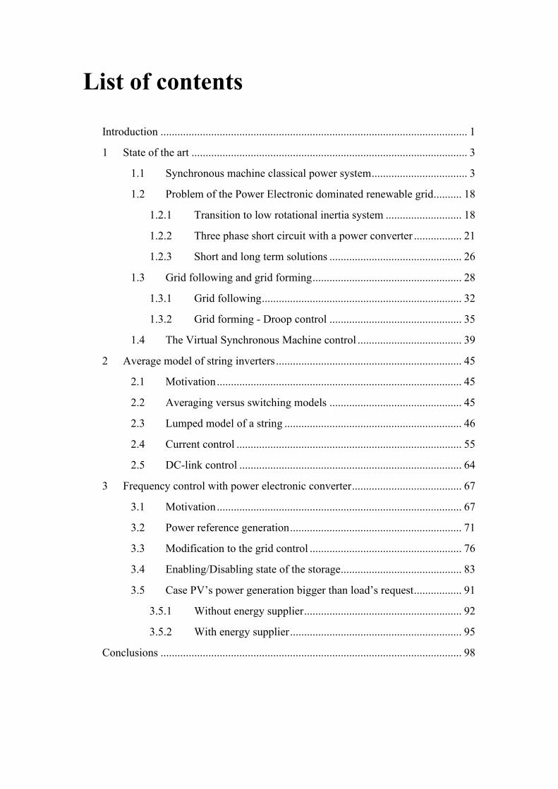
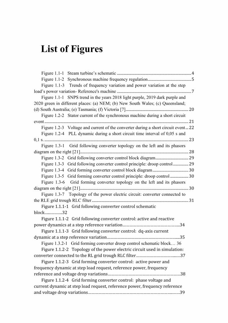