Preprint typeset in JHEP style - HYPER VERSION January 2009

String Theory

University of Cambridge Part III Mathematical Tripos

Dr David Tong

Department of Applied Mathematics and Theoretical Physics,

Centre for Mathematical Sciences,

Wilberforce Road,

Cambridge, CB3 OWA, UK

http://www.damtp.cam.ac.uk/user/tong/string.html

d.tong@damtp.cam.ac.uk

– 1 –

Recommended Books and Resources

• J. Polchinski, String Theory

This two volume work is the standard introduction to the subject. Our lectures will

more or less follow the path laid down in volume one covering the bosonic string. The

book contains explanations and descriptions of many details that have been deliberately

(and, I suspect, at times inadvertently) swept under a very large rug in these lectures.

Volume two covers the superstring.

• M. Green, J. Schwarz and E. Witten, Superstring Theory

Another two volume set. It is now over 20 years old and takes a slightly old-fashioned

route through the subject, with no explicit mention of conformal field theory. How-

ever, it does contain much good material and the explanations are uniformly excellent.

Volume one is most relevant for these lectures.

• B. Zwiebach, A First Course in String Theory

This book grew out of a course given to undergraduates who had no previous exposure

to general relativity or quantum field theory. It has wonderful pedagogical discussions

of the basics of lightcone quantization. More surprisingly, it also has some very clear

descriptions of several advanced topics, even though it misses out all the bits in between.

• P. Di Francesco, P. Mathieu and D. Senechal, Conformal Field Theory

This big yellow book is a↵ectionately known as the yellow pages. It’s a great way

to learn conformal field theory. At first glance, it comes across as slightly daunting

because it’s big. (And yellow). But you soon realise that it’s big because it starts at

the beginning and provides detailed explanations at every step. The material necessary

for this course can be found in chapters 5 and 6.

Further References: “String Theory and M-Theory” by Becker, Becker and Schwarz

and “String Theory in a Nutshell” (it’s a big nutshell) by Kiritsis both deal with the

bosonic string fairly quickly, but include more advanced topics that may be of interest.

The book “D-Branes” by Johnson has lively and clear discussions about the many joys

of D-branes. Links to several excellent online resources, including video lectures by

Shiraz Minwalla, are listed on the course webpage.

Contents

0. Introduction 1

0.1 Quantum Gravity 3

1. The Relativistic String 9

1.1 The Relativistic Point Particle 9

1.1.1 Quantization 11

1.1.2 Ein Einbein 13

1.2 The Nambu-Goto Action 14

1.2.1 Symmetries of the Nambu-Goto Action 17

1.2.2 Equations of Motion 18

1.3 The Polyakov Action 18

1.3.1 Symmetries of the Polyakov Action 20

1.3.2 Fixing a Gauge 22

1.4 Mode Expansions 25

1.4.1 The Constraints Revisited 26

2. The Quantum String 28

2.1 A Lightning Look at Covariant Quantization 28

2.1.1 Ghosts 30

2.1.2 Constraints 30

2.2 Lightcone Quantization 32

2.2.1 Lightcone Gauge 33

2.2.2 Quantization 36

2.3 The String Spectrum 40

2.3.1 The Tachyon 40

2.3.2 The First Excited States 41

2.3.3 Higher Excited States 45

2.4 Lorentz Invariance Revisited 46

2.5 A Nod to the Superstring 48

3. Open Strings and D-Branes 50

3.1 Quantization 53

3.1.1 The Ground State 54

3.1.2 First Excited States: A World of Light 55

– 1 –

3.1.3 Higher Excited States and Regge Trajectories 56

3.1.4 Another Nod to the Superstring 56

3.2 Brane Dynamics: The Dirac Action 57

3.3 Multiple Branes: A World of Glue 59

4. Introducing Conformal Field Theory 61

4.0.1 Euclidean Space 62

4.0.2 The Holomorphy of Conformal Transformations 63

4.1 Classical Aspects 63

4.1.1 The Stress-Energy Tensor 64

4.1.2 Noether Currents 66

4.1.3 An Example: The Free Scalar Field 67

4.2 Quantum Aspects 68

4.2.1 Operator Product Expansion 68

4.2.2 Ward Identities 70

4.2.3 Primary Operators 73

4.3 An Example: The Free Scalar Field 77

4.3.1 The Propagator 77

4.3.2 An Aside: No Goldstone Bosons in Two Dimensions 79

4.3.3 The Stress-Energy Tensor and Primary Operators 80

4.4 The Central Charge 82

4.4.1 c is for Casimir 84

4.4.2 The Weyl Anomaly 86

4.4.3 c is for Cardy 89

4.4.4 c has a Theorem 91

4.5 The Virasoro Algebra 92

4.5.1 Radial Quantization 92

4.5.2 The Virasoro Algebra 94

4.5.3 Representations of the Virasoro Algebra 96

4.5.4 Consequences of Unitarity 98

4.6 The State-Operator Map 99

4.6.1 Some Simple Consequences 101

4.6.2 Our Favourite Example: The Free Scalar Field 102

4.7 Brief Comments on Conformal Field Theories with Boundaries 105

5. The Polyakov Path Integral and Ghosts 108

5.1 The Path Integral 108

5.1.1 The Faddeev-Popov Method 109

– 2 –

5.1.2 The Faddeev-Popov Determinant 112

5.1.3 Ghosts 113

5.2 The Ghost CFT 114

5.3 The Critical “Dimension” of String Theory 117

5.3.1 The Usual Nod to the Superstring 118

5.3.2 An Aside: Non-Critical Strings 119

5.4 States and Vertex Operators 120

5.4.1 An Example: Closed Strings in Flat Space 122

5.4.2 An Example: Open Strings in Flat Space 123

5.4.3 More General CFTs 124

6. String Interactions 125

6.1 What to Compute? 125

6.1.1 Summing Over Topologies 127

6.2 Closed String Amplitudes at Tree Level 130

6.2.1 Remnant Gauge Symmetry: SL(2,C) 130

6.2.2 The Virasoro-Shapiro Amplitude 132

6.2.3 Lessons to Learn 135

6.3 Open String Scattering 139

6.3.1 The Veneziano Amplitude 141

6.3.2 The Tension of D-Branes 142

6.4 One-Loop Amplitudes 143

6.4.1 The Moduli Space of the Torus 143

6.4.2 The One-Loop Partition Function 146

6.4.3 Interpreting the String Partition Function 149

6.4.4 So is String Theory Finite? 152

6.4.5 Beyond Perturbation Theory? 153

6.5 Appendix: Games with Integrals and Gamma Functions 154

7. Low Energy E↵ective Actions 157

7.1 Einstein’s Equations 158

7.1.1 The Beta Function 159

7.1.2 Ricci Flow 163

7.2 Other Couplings 163

7.2.1 Charged Strings and the B field 163

7.2.2 The Dilaton 165

7.2.3 Beta Functions 167

7.3 The Low-Energy E↵ective Action 167

– 3 –

7.3.1 String Frame and Einstein Frame 168

7.3.2 Corrections to Einstein’s Equations 170

7.3.3 Nodding Once More to the Superstring 171

7.4 Some Simple Solutions 173

7.4.1 Compactifications 174

7.4.2 The String Itself 175

7.4.3 Magnetic Branes 177

7.4.4 Moving Away from the Critical Dimension 180

7.4.5 The Elephant in the Room: The Tachyon 183

7.5 D-Branes Revisited: Background Gauge Fields 183

7.5.1 The Beta Function 184

7.5.2 The Born-Infeld Action 187

7.6 The DBI Action 188

7.6.1 Coupling to Closed String Fields 189

7.7 The Yang-Mills Action 191

7.7.1 D-Branes in Type II Superstring Theories 195

8. Compactification and T-Duality 197

8.1 The View from Spacetime 197

8.1.1 Moving around the Circle 199

8.2 The View from the Worldsheet 200

8.2.1 Massless States 202

8.2.2 Charged Fields 202

8.2.3 Enhanced Gauge Symmetry 203

8.3 Why Big Circles are the Same as Small Circles 204

8.3.1 A Path Integral Derivation of T-Duality 206

8.3.2 T-Duality for Open Strings 207

8.3.3 T-Duality for Superstrings 208

8.3.4 Mirror Symmetry 208

8.4 Epilogue 209

– 4 –

Acknowledgements

These lectures are aimed at beginning graduate students. They assume a working

knowledge of quantum field theory and general relativity. The lectures were given over

one semester and are based broadly on Volume one of the book by Joe Polchinski. I

inherited the course from Michael Green whose notes were extremely useful. I also

benefited enormously from the insightful and entertaining video lectures by Shiraz

Minwalla.

I’m grateful to Anirban Basu, Niklas Beisert, Joe Bhaseen, Diego Correa, Nick Dorey,

Michael Green, Anshuman Maharana, Malcolm Perry and Martin Schnabl for discus-

sions and help with various aspects of these notes. I’m also grateful to the students,

especially Carlos Guedes, for their excellent questions and superhuman typo-spotting

abilities. Finally, my thanks to Alex Considine for infinite patience and understanding

over the weeks these notes were written. I am supported by the Royal Society.

– 5 –

0. Introduction

String theory is an ambitious project. It purports to be an all-encompassing theory

of the universe, unifying the forces of Nature, including gravity, in a single quantum

mechanical framework.

The premise of string theory is that, at the fundamental level, matter does not consist

of point-particles but rather of tiny loops of string. From this slightly absurd beginning,

the laws of physics emerge. General relativity, electromagnetism and Yang-Mills gauge

theories all appear in a surprising fashion. However, they come with baggage. String

theory gives rise to a host of other ingredients, most strikingly extra spatial dimensions

of the universe beyond the three that we have observed. The purpose of this course is

to understand these statements in detail.

These lectures di↵er from most other courses that you will take in a physics degree.

String theory is speculative science. There is no experimental evidence that string

theory is the correct description of our world and scant hope that hard evidence will

arise in the near future. Moreover, string theory is very much a work in progress and

certain aspects of the theory are far from understood. Unresolved issues abound and

it seems likely that the final formulation has yet to be written. For these reasons, I’ll

begin this introduction by suggesting some answers to the question: Why study string

theory?

Reason 1. String theory is a theory of quantum gravity

String theory unifies Einstein’s theory of general relativity with quantum mechanics.

Moreover, it does so in a manner that retains the explicit connection with both quantum

theory and the low-energy description of spacetime.

But quantum gravity contains many puzzles, both technical and conceptual. What

does spacetime look like at the shortest distance scales? How can we understand

physics if the causal structure fluctuates quantum mechanically? Is the big bang truely

the beginning of time? Do singularities that arise in black holes really signify the end

of time? What is the microscopic origin of black hole entropy and what is it telling

us? What is the resolution to the information paradox? Some of these issues will be

reviewed later in this introduction.

Whether or not string theory is the true description of reality, it o↵ers a framework

in which one can begin to explore these issues. For some questions, string theory

has given very impressive and compelling answers. For others, string theory has been

almost silent.

– 1 –

Reason 2. String theory may be the theory of quantum gravity

With broad brush, string theory looks like an extremely good candidate to describe the

real world. At low-energies it naturally gives rise to general relativity, gauge theories,

scalar fields and chiral fermions. In other words, it contains all the ingredients that

make up our universe. It also gives the only presently credible explanation for the value

of the cosmological constant although, in fairness, I should add that the explanation is

so distasteful to some that the community is rather amusingly split between whether

this is a good thing or a bad thing. Moreover, string theory incorporates several ideas

which do not yet have experimental evidence but which are considered to be likely

candidates for physics beyond the standard model. Prime examples are supersymmetry

and axions.

However, while the broad brush picture looks good, the finer details have yet to

be painted. String theory does not provide unique predictions for low-energy physics

but instead o↵ers a bewildering array of possibilities, mostly dependent on what is

hidden in those extra dimensions. Partly, this problem is inherent to any theory of

quantum gravity: as we’ll review shortly, it’s a long way down from the Planck scale

to the domestic energy scales explored at the LHC. Using quantum gravity to extract

predictions for particle physics is akin to using QCD to extract predictions for how

co↵ee makers work. But the mere fact that it’s hard is little comfort if we’re looking

for convincing evidence that string theory describes the world in which we live.

While string theory cannot at present o↵er falsifiable predictions, it has nonetheless

inspired new and imaginative proposals for solving outstanding problems in particle

physics and cosmology. There are scenarios in which string theory might reveal itself

in forthcoming experiments. Perhaps we’ll find extra dimensions at the LHC, perhaps

we’ll see a network of fundamental strings stretched across the sky, or perhaps we’ll

detect some feature of non-Gaussianity in the CMB that is characteristic of D-branes

at work during inflation. My personal feeling however is that each of these is a long

shot and we may not know whether string theory is right or wrong within our lifetimes.

Of course, the history of physics is littered with naysayers, wrongly suggesting that

various theories will never be testable. With luck, I’ll be one of them.

Reason 3. String theory provides new perspectives on gauge theories

String theory was born from attempts to understand the strong force. Almost forty

years later, this remains one of the prime motivations for the subject. String theory

provides tools with which to analyze down-to-earth aspects of quantum field theory

that are far removed from high-falutin’ ideas about gravity and black holes.

– 2 –

Of immediate relevance to this course are the pedagogical reasons to invest time in

string theory. At heart, it is the study of conformal field theory and gauge symmetry.

The techniques that we’ll learn are not isolated to string theory, but apply to countless

systems which have direct application to real world physics.

On a deeper level, string theory provides new and very surprising methods to under-

stand aspects of quantum gauge theories. Of these, the most startling is the AdS/CFT

correspondence, first conjectured by Juan Maldacena, which gives a relationship be-

tween strongly coupled quantum field theories and gravity in higher dimensions. These

ideas have been applied in areas ranging from nuclear physics to condensed matter

physics and have provided qualitative (and arguably quantitative) insights into strongly

coupled phenomena.

Reason 4. String theory provides new results in mathematics

For the past 250 years, the close relationship between mathematics and physics has

been almost a one-way street: physicists borrowed many things from mathematicians

but, with a few noticeable exceptions, gave little back. In recent times, that has

changed. Ideas and techniques from string theory and quantum field theory have been

employed to give new “proofs” and, perhaps more importantly, suggest new directions

and insights in mathematics. The most well known of these is mirror symmetry, a

relationship between topologically di↵erent Calabi-Yau manifolds.

The four reasons described above also crudely characterize the string theory commu-

nity: there are “relativists” and “phenomenologists” and “field theorists” and “math-

ematicians”. Of course, the lines between these di↵erent sub-disciplines are not fixed

and one of the great attractions of string theory is its ability to bring together people

working in di↵erent areas — from cosmology to condensed matter to pure mathematics

— and provide a framework in which they can profitably communicate. In my opinion,

it is this cross-fertilization between fields which is the greatest strength of string theory.

0.1 Quantum Gravity

This is a starter course in string theory. Our focus will be on the perturbative approach

to the bosonic string and, in particular, why this gives a consistent theory of quantum

gravity. Before we leap into this, it is probably best to say a few words about quantum

gravity itself. Like why it’s hard. And why it’s important. (And why it’s not).

The Einstein Hilbert action is given by

SEH =1

16⇡GN

Zd4x

p�gR

– 3 –

Newton’s constant GN can be written as

8⇡GN =~cM2

pl

Throughout these lectures we work in units with ~ = c = 1. The Planck mass Mpl

defines an energy scale

Mpl ⇡ 2⇥ 1018 GeV .

(This is sometimes referred to as the reduced Planck mass, to distinguish it from the

scale without the factor of 8⇡, namelyp1/GN ⇡ 1⇥ 1019 GeV).

There are a couple of simple lessons that we can already take from this. The first is

that the relevant coupling in the quantum theory is 1/Mpl. To see that this is indeed

the case from the perspective of the action, we consider small perturbations around flat

Minkowski space,

gµ⌫ = ⌘µ⌫ +1

Mpl

hµ⌫

The factor of 1/Mpl is there to ensure that when we expand out the Einstein-Hilbert

action, the kinetic term for h is canonically normalized, meaning that it comes with no

powers of Mpl. This then gives the kind of theory that you met in your first course on

quantum field theory, albeit with an infinite series of interaction terms,

SEH =

Zd4x (@h)2 +

1

Mpl

h (@h)2 +1

M2

pl

h2 (@h)2 + . . .

Each of these terms is schematic: if you were to do this explicitly, you would find a

mess of indices contracted in di↵erent ways. We see that the interactions are suppressed

by powers of Mpl. This means that quantum perturbation theory is an expansion in

the dimensionless ratio E2/M2

pl, where E is the energy associated to the process of

interest. We learn that gravity is weak, and therefore under control, at low-energies.

But gravitational interactions become strong as the energy involved approaches the

Planck scale. In the language of the renormalization group, couplings of this type are

known as irrelevant.

The second lesson to take away is that the Planck scale Mpl is very very large. The

LHC will probe the electroweak scale,MEW ⇠ 103 GeV. The ratio isMEW/Mpl ⇠ 10�15.

For this reason, quantum gravity will not a↵ect your daily life, even if your daily life

involves the study of the most extreme observable conditions in the universe.

– 4 –

Gravity is Non-Renormalizable

Quantum field theories with irrelevant couplings are typically ill-behaved at high-

energies, rendering the theory ill-defined. Gravity is no exception. Theories of this

type are called non-renormalizable, which means that the divergences that appear in

the Feynman diagram expansion cannot be absorbed by a finite number of countert-

erms. In pure Einstein gravity, the symmetries of the theory are enough to ensure that

the one-loop S-matrix is finite. The first divergence occurs at two-loops and requires

the introduction of a counterterm of the form,

� ⇠ 1

✏

1

M4

pl

Zd4x

p�gRµ⌫

⇢�R⇢��R�

µ⌫

with ✏ = 4�D. All indications point towards the fact that this is the first in an infinite

number of necessary counterterms.

Coupling gravity to matter requires an interaction term of the form,

Sint =

Zd4x

1

Mpl

hµ⌫Tµ⌫ +O(h2)

This makes the situation marginally worse, with the first diver-

Figure 1:

gence now appearing at one-loop. The Feynman diagram in the

figure shows particle scattering through the exchange of two gravi-

tons. When the momentum k running in the loop is large, the

diagram is badly divergent: it scales as

1

M4

pl

Z 1d4k

Non-renormalizable theories are commonplace in the history of physics, the most com-

monly cited example being Fermi’s theory of the weak interaction. The first thing to say

about them is that they are far from useless! Non-renormalizable theories are typically

viewed as e↵ective field theories, valid only up to some energy scale ⇤. One deals with

the divergences by simply admitting ignorance beyond this scale and treating ⇤ as a

UV cut-o↵ on any momentum integral. In this way, we get results which are valid to an

accuracy of E/⇤ (perhaps raised to some power). In the case of the weak interaction,

Fermi’s theory accurately predicts physics up to an energy scale ofp1/GF ⇠ 100 GeV.

In the case of quantum gravity, Einstein’s theory works to an accuracy of (E/Mpl)2.

– 5 –

However, non-renormalizable theories are typically unable to describe physics at their

cut-o↵ scale ⇤ or beyond. This is because they are missing the true ultra-violet degrees

of freedom which tame the high-energy behaviour. In the case of the weak force, these

new degrees of freedom are the W and Z bosons. We would like to know what missing

degrees of freedom are needed to complete gravity.

Singularities

Only a particle physicist would phrase all questions about the universe in terms of

scattering amplitudes. In general relativity we typically think about the geometry as

a whole, rather than bastardizing the Einstein-Hilbert action and discussing perturba-

tions around flat space. In this language, the question of high-energy physics turns into

one of short distance physics. Classical general relativity is not to be trusted in regions

where the curvature of spacetime approaches the Planck scale and ultimately becomes

singular. A quantum theory of gravity should resolve these singularities.

The question of spacetime singularities is morally equivalent to that of high-energy

scattering. Both probe the ultra-violet nature of gravity. A spacetime geometry is

made of a coherent collection of gravitons, just as the electric and magnetic fields in a

laser are made from a collection of photons. The short distance structure of spacetime

is governed – after Fourier transform – by high momentum gravitons. Understanding

spacetime singularities and high-energy scattering are di↵erent sides of the same coin.

There are two situations in general relativity where singularity theorems tell us that

the curvature of spacetime gets large: at the big bang and in the center of a black hole.

These provide two of the biggest challenges to any putative theory of quantum gravity.

Gravity is Subtle

It is often said that general relativity contains the seeds of its own destruction. The

theory is unable to predict physics at the Planck scale and freely admits to it. Problems

such as non-renormalizability and singularities are, in a Rumsfeldian sense, known

unknowns. However, the full story is more complicated and subtle. On the one hand,

the issue of non-renormalizability may not quite be the crisis that it first appears. On

the other hand, some aspects of quantum gravity suggest that general relativity isn’t

as honest about its own failings as is usually advertised. The theory hosts a number of

unknown unknowns, things that we didn’t even know that we didn’t know. We won’t

have a whole lot to say about these issues in this course, but you should be aware of

them. Here I mention only a few salient points.

– 6 –

Firstly, there is a key di↵erence between Fermi’s theory of the weak interaction and

gravity. Fermi’s theory was unable to provide predictions for any scattering process

at energies abovep

1/GF . In contrast, if we scatter two objects at extremely high-

energies in gravity — say, at energies E � Mpl — then we know exactly what will

happen: we form a big black hole. We don’t need quantum gravity to tell us this.

Classical general relativity is su�cient. If we restrict attention to scattering, the crisis

of non-renormalizability is not problematic at ultra-high energies. It’s troublesome only

within a window of energies around the Planck scale.

Similar caveats hold for singularities. If you are foolish enough to jump into a black

hole, then you’re on your own: without a theory of quantum gravity, no one can tell you

what fate lies in store at the singularity. Yet, if you are smart and stay outside of the

black hole, you’ll be hard pushed to see any e↵ects of quantum gravity. This is because

Nature has conspired to hide Planck scale curvatures from our inquisitive eyes. In the

case of black holes this is achieved through cosmic censorship which is a conjecture in

classical general relativity that says singularities are hidden behind horizons. In the

case of the big bang, it is achieved through inflation, washing away any traces from the

very early universe. Nature appears to shield us from the e↵ects of quantum gravity,

whether in high-energy scattering or in singularities. I think it’s fair to say that no one

knows if this conspiracy is pointing at something deep, or is merely inconvenient for

scientists trying to probe the Planck scale.

While horizons may protect us from the worst excesses of singularities, they come

with problems of their own. These are the unknown unknowns: di�culties that arise

when curvatures are small and general relativity says “trust me”. The entropy of black

holes and the associated paradox of information loss strongly suggest that local quan-

tum field theory breaks down at macroscopic distance scales. Attempts to formulate

quantum gravity in de Sitter space, or in the presence of eternal inflation, hint at similar

di�culties. Ideas of holography, black hole complimentarity and the AdS/CFT corre-

spondence all point towards non-local e↵ects and the emergence of spacetime. These are

the deep puzzles of quantum gravity and their relationship to the ultra-violet properties

of gravity is unclear.

As a final thought, let me mention the one observation that has an outside chance of

being related to quantum gravity: the cosmological constant. With an energy scale of

⇤ ⇠ 10�3 eV it appears to have little to do with ultra-violet physics. If it does have its

origins in a theory of quantum gravity, it must either be due to some subtle “unknown

unknown”, or because it is explained away as an environmental quantity as in string

theory.

– 7 –

Is the Time Ripe?

Our current understanding of physics, embodied in the standard model, is valid up to

energy scales of 103 GeV. This is 15 orders of magnitude away from the Planck scale.

Why do we think the time is now ripe to tackle quantum gravity? Surely we are like

the ancient Greeks arguing about atomism. Why on earth do we believe that we’ve

developed the right tools to even address the question?

The honest answer, I think, is hubris.

Figure 2:

However, there is mild circumstantial evidence

that the framework of quantum field theory might

hold all the way to the Planck scale without any-

thing very dramatic happening in between. The

main argument is unification. The three coupling

constants of Nature run logarithmically, meeting

miraculously at the GUT energy scale of 1015 GeV.

Just slightly later, the fourth force of Nature, grav-

ity, joins them. While not overwhelming, this does

provide a hint that perhaps quantum field theory

can be taken seriously at these ridiculous scales.

Historically I suspect this was what convinced large parts of the community that it was

ok to speak about processes at 1018 GeV.

Finally, perhaps the most compelling argument for studying physics at the Planck

scale is that string theory does provide a consistent unified quantum theory of gravity

and the other forces. Given that we have this theory sitting in our laps, it would be

foolish not to explore its consequences. The purpose of these lecture notes is to begin

this journey.

– 8 –

1. The Relativistic String

All lecture courses on string theory start with a discussion of the point particle. Ours

is no exception. We’ll take a flying tour through the physics of the relativistic point

particle and extract a couple of important lessons that we’ll take with us as we move

onto string theory.

1.1 The Relativistic Point Particle

We want to write down the Lagrangian describing a relativistic particle of mass m.

In anticipation of string theory, we’ll consider D-dimensional Minkowski space R1,D�1.

Throughout these notes, we work with signature

⌘µ⌫ = diag(�1,+1,+1, . . . ,+1)

Note that this is the opposite signature to my quantum field theory notes.

If we fix a frame with coordinates Xµ = (t, ~x) the action is simple:

S = �m

Zdt

q1� ~x · ~x . (1.1)

To see that this is correct we can compute the momentum ~p, conjugate to ~x, and the

energy E which is equal to the Hamiltonian,

~p =m~xp

1� ~x · ~x, E =

pm2 + ~p2 ,

both of which should be familiar from courses on special relativity.

Although the Lagrangian (1.1) is correct, it’s not fully satisfactory. The reason is

that time t and space ~x play very di↵erent roles in this Lagrangian. The position ~x is

a dynamical degree of freedom. In contrast, time t is merely a parameter providing a

label for the position. Yet Lorentz transformations are supposed to mix up t and ~x and

such symmetries are not completely obvious in (1.1). Can we find a new Lagrangian

in which time and space are on equal footing?

One possibility is to treat both time and space as labels. This leads us to the

concept of field theory. However, in this course we will be more interested in the other

possibility: we will promote time to a dynamical degree of freedom. At first glance,

this may appear odd: the number of degrees of freedom is one of the crudest ways we

have to characterize a system. We shouldn’t be able to add more degrees of freedom

– 9 –

at will without fundamentally changing the system that we’re talking about. Another

way of saying this is that the particle has the option to move in space, but it doesn’t

have the option to move in time. It has to move in time. So we somehow need a way

to promote time to a degree of freedom without it really being a true dynamical degree

of freedom! How do we do this? The answer, as we will now show, is gauge symmetry.

Consider the action,X

X

0

Figure 3:

S = �m

Zd⌧q

�XµX⌫⌘µ⌫ , (1.2)

where µ = 0, . . . , D � 1 and Xµ = dXµ/d⌧ . We’ve introduced a

new parameter ⌧ which labels the position along the worldline of

the particle as shown by the dashed lines in the figure. This action

has a simple interpretation: it is just the proper timeRds along the

worldline.

Naively it looks as if we now have D physical degrees of freedom rather than D � 1

because, as promised, the time direction X0 ⌘ t is among our dynamical variables:

X0 = X0(⌧). However, this is an illusion. To see why, we need to note that the action

(1.2) has a very important property: reparameterization invariance. This means that

we can pick a di↵erent parameter ⌧ on the worldline, related to ⌧ by any monotonic

function

⌧ = ⌧(⌧) .

Let’s check that the action is invariant under transformations of this type. The inte-

gration measure in the action changes as d⌧ = d⌧ |d⌧/d⌧ |. Meanwhile, the velocities

change as dXµ/d⌧ = (dXµ/d⌧) (d⌧/d⌧). Putting this together, we see that the action

can just as well be written in the ⌧ reparameterization,

S = �m

Zd⌧

r�dXµ

d⌧

dX⌫

d⌧⌘µ⌫ .

The upshot of this is that not all D degrees of freedom Xµ are physical. For example,

suppose you find a solution to this system, so that you know how X0 changes with

⌧ and how X1 changes with ⌧ and so on. Not all of that information is meaningful

because ⌧ itself is not meaningful. In particular, we could use our reparameterization

invariance to simply set

⌧ = X0(⌧) ⌘ t (1.3)

– 10 –

If we plug this choice into the action (1.2) then we recover our initial action (1.1). The

reparameterization invariance is a gauge symmetry of the system. Like all gauge sym-

metries, it’s not really a symmetry at all. Rather, it is a redundancy in our description.

In the present case, it means that although we seem to have D degrees of freedom Xµ,

one of them is fake.

The fact that one of the degrees of freedom is a fake also shows up if we look at the

momenta,

pµ =@L

@Xµ=

mX⌫⌘µ⌫q�X�X⇢ ⌘�⇢

(1.4)

These momenta aren’t all independent. They satisfy

pµpµ +m2 = 0 (1.5)

This is a constraint on the system. It is, of course, the mass-shell constraint for a

relativistic particle of mass m. From the worldline perspective, it tells us that the

particle isn’t allowed to sit still in Minkowski space: at the very least, it had better

keep moving in a timelike direction with (p0)2 � m2.

One advantage of the action (1.2) is that the Poincare symmetry of the particle is

now manifest, appearing as a global symmetry on the worldline

Xµ ! ⇤µ⌫X

⌫ + cµ (1.6)

where ⇤ is a Lorentz transformation satisfying ⇤µ⌫⌘

⌫⇢⇤�⇢ = ⌘µ�, while cµ corresponds

to a constant translation. We have made all the symmetries manifest at the price of

introducing a gauge symmetry into our system. A similar gauge symmetry will arise

in the relativistic string and much of this course will be devoted to understanding its

consequences.

1.1.1 Quantization

It’s a trivial matter to quantize this action. We introduce a wavefunction (X). This

satisfies the usual Schrodinger equation,

i@

@⌧= H .

But, computing the Hamiltonian H = Xµpµ�L, we find that it vanishes: H = 0. This

shouldn’t be surprising. It is simply telling us that the wavefunction doesn’t depend on

– 11 –

⌧ . Since the wavefunction is something physical while, as we have seen, ⌧ is not, this is

to be expected. Note that this doesn’t mean that time has dropped out of the problem.

On the contrary, in this relativistic context, time X0 is an operator, just like the spatial

coordinates ~x. This means that the wavefunction is immediately a function of space

and time. It is not like a static state in quantum mechanics, but more akin to the fully

integrated solution to the non-relativistic Schrodinger equation.

The classical system has a constraint given by (1.5). In the quantum theory, we

impose this constraint as an operator equation on the wavefunction, namely (pµpµ +

m2) = 0. Using the usual representation of the momentum operator pµ = �i@/@Xµ,

we recognize this constraint as the Klein-Gordon equation✓� @

@Xµ

@

@X⌫⌘µ⌫ +m2

◆ (X) = 0 (1.7)

Although this equation is familiar from field theory, it’s important to realize that the

interpretation is somewhat di↵erent. In relativistic field theory, the Klein-Gordon equa-

tion is the equation of motion obeyed by a scalar field. In relativistic quantum mechan-

ics, it is the equation obeyed by the wavefunction. In the early days of field theory,

the fact that these two equations are the same led people to think one should view

the wavefunction as a classical field and quantize it a second time. This isn’t cor-

rect, but nonetheless the language has stuck and it is common to talk about the point

particle perspective as “first quantization” and the field theory perspective as “second

quantization”.

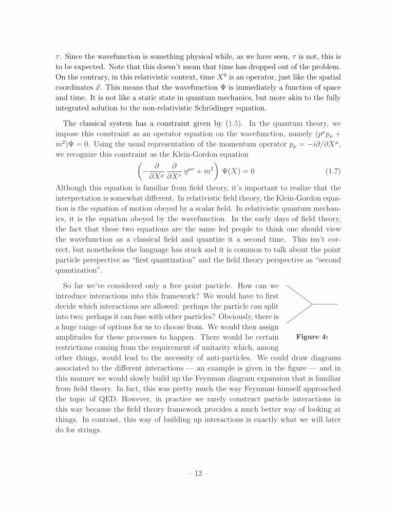
So far we’ve considered only a free point particle. How can we

Figure 4:

introduce interactions into this framework? We would have to first

decide which interactions are allowed: perhaps the particle can split

into two; perhaps it can fuse with other particles? Obviously, there is

a huge range of options for us to choose from. We would then assign

amplitudes for these processes to happen. There would be certain

restrictions coming from the requirement of unitarity which, among

other things, would lead to the necessity of anti-particles. We could draw diagrams

associated to the di↵erent interactions — an example is given in the figure — and in

this manner we would slowly build up the Feynman diagram expansion that is familiar

from field theory. In fact, this was pretty much the way Feynman himself approached

the topic of QED. However, in practice we rarely construct particle interactions in

this way because the field theory framework provides a much better way of looking at

things. In contrast, this way of building up interactions is exactly what we will later

do for strings.

– 12 –

1.1.2 Ein Einbein

There is another action that describes the relativistic point particle. We introduce yet

another field on the worldline, e(⌧), and write

S =1

2

Zd⌧⇣e�1X2 � em2

⌘, (1.8)

where we’ve used the notation X2 = XµX⌫⌘µ⌫ . For the rest of these lectures, terms

like X2 will always mean an implicit contraction with the spacetime Minkowski metric.

This form of the action makes it look as if we have coupled the worldline theory to

1d gravity, with the field e(⌧) acting as an einbein (in the sense of vierbeins that are

introduced in general relativity). To see this, note that we could change notation and

write this action in the more suggestive form

S = �1

2

Zd⌧

p�g⌧⌧

⇣g⌧⌧X2 +m2

⌘. (1.9)

where g⌧⌧ = (g⌧⌧ )�1 is the metric on the worldline and e =p�g⌧⌧

Although our action appears to have one more degree of freedom, e, it can be easily

checked that it has the same equations of motion as (1.2). The reason for this is that

e is completely fixed by its equation of motion, X2 + e2m2 = 0. Substituting this into

the action (1.8) recovers (1.2)

The action (1.8) has a couple of advantages over (1.2). Firstly, it works for massless

particles with m = 0. Secondly, the absence of the annoying square root means that

it’s easier to quantize in a path integral framework.

The action (1.8) retains invariance under reparameterizations which are now written

in a form that looks more like general relativity. For transformations parameterized by

an infinitesimal ⌘, we have

⌧ ! ⌧ = ⌧ � ⌘(⌧) , �e =d

d⌧(⌘(⌧)e) , �Xµ =

dXµ

d⌧⌘(⌧) (1.10)

The einbein e transforms as a density on the worldline, while each of the coordinates

Xµ transforms as a worldline scalar.

– 13 –

1.2 The Nambu-Goto Action

A particle sweeps out a worldline in Minkowski space. A string

σ

τ

Figure 5:

sweeps out a worldsheet. We’ll parameterize this worldsheet by

one timelike coordinate ⌧ , and one spacelike coordinate �. In this

section we’ll focus on closed strings and take � to be periodic,

with range

� 2 [0, 2⇡) . (1.11)

We will sometimes package the two worldsheet coordinates to-

gether as �↵ = (⌧, �), ↵ = 0, 1. Then the string sweeps out a

surface in spacetime which defines a map from the worldsheet to

Minkowski space, Xµ(�, ⌧) with µ = 0, . . . , D � 1. For closed strings, we require

Xµ(�, ⌧) = Xµ(� + 2⇡, ⌧) .

In this context, spacetime is sometimes referred to as the target space to distinguish it

from the worldsheet.

We need an action that describes the dynamics of this string. The key property

that we will ask for is that nothing depends on the coordinates �↵ that we choose

on the worldsheet. In other words, the string action should be reparameterization

invariant. What kind of action does the trick? Well, for the point particle the action

was proportional to the length of the worldline. The obvious generalization is that the

action for the string should be proportional to the area, A, of the worldsheet. This

is certainly a property that is characteristic of the worldsheet itself, rather than any

choice of parameterization.

How do we find the area A in terms of the coordinates Xµ(�, ⌧)? The worldsheet is

a curved surface embedded in spacetime. The induced metric, �↵�, on this surface is

the pull-back of the flat metric on Minkowski space,

�↵� =@Xµ

@�↵

@X⌫

@��⌘µ⌫ . (1.12)

Then the action which is proportional to the area of the worldsheet is given by,

S = �T

Zd2�

p� det � . (1.13)

Here T is a constant of proportionality. We will see shortly that it is the tension of the

string, meaning the mass per unit length.

– 14 –

We can write this action a little more explicitly. The pull-back of the metric is given

by,

�↵� =

X2 X ·X 0

X ·X 0 X 02

!.

where Xµ = @Xµ/@⌧ and Xµ 0 = @Xµ/@�. The action then takes the form,

S = �T

Zd2�q

�(X)2 (X 0)2 + (X ·X 0)2 . (1.14)

This is the Nambu-Goto action for a relativistic string.

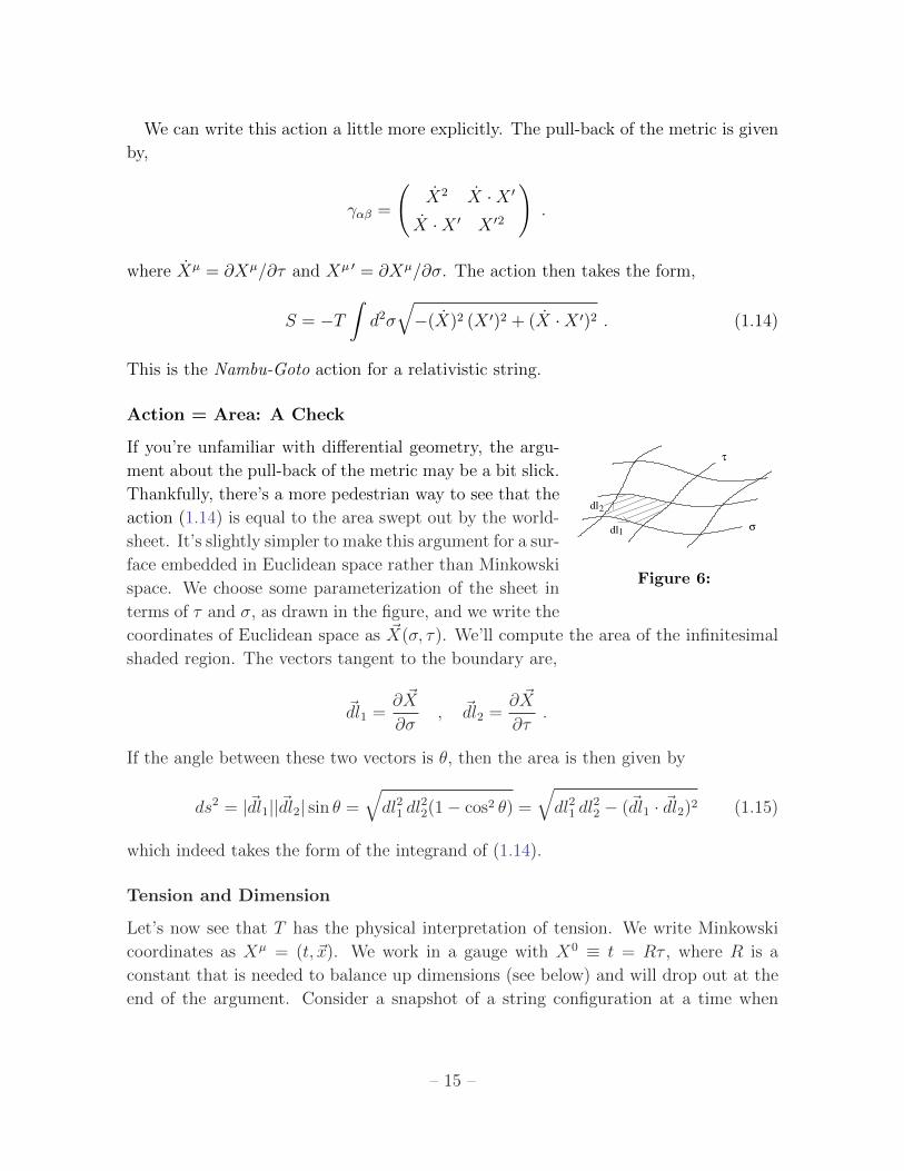
Action = Area: A Check

If you’re unfamiliar with di↵erential geometry, the argu-

dl

dl

1

2

τ

σ

Figure 6:

ment about the pull-back of the metric may be a bit slick.

Thankfully, there’s a more pedestrian way to see that the

action (1.14) is equal to the area swept out by the world-

sheet. It’s slightly simpler to make this argument for a sur-

face embedded in Euclidean space rather than Minkowski

space. We choose some parameterization of the sheet in

terms of ⌧ and �, as drawn in the figure, and we write the

coordinates of Euclidean space as ~X(�, ⌧). We’ll compute the area of the infinitesimal

shaded region. The vectors tangent to the boundary are,

~dl1

=@ ~X

@�, ~dl

2

=@ ~X

@⌧.

If the angle between these two vectors is ✓, then the area is then given by

ds2 = |~dl1

||~dl2

| sin ✓ =q

dl21

dl22

(1� cos2 ✓) =qdl2

1

dl22

� (~dl1

· ~dl2

)2 (1.15)

which indeed takes the form of the integrand of (1.14).

Tension and Dimension

Let’s now see that T has the physical interpretation of tension. We write Minkowski

coordinates as Xµ = (t, ~x). We work in a gauge with X0 ⌘ t = R⌧ , where R is a

constant that is needed to balance up dimensions (see below) and will drop out at the

end of the argument. Consider a snapshot of a string configuration at a time when

– 15 –

d~x/d⌧ = 0 so that the instantaneous kinetic energy vanishes. Evaluating the action for

a time dt gives

S = �T

Zd⌧d�R

p(d~x/d�)2 = �T

Zdt (spatial length of string) . (1.16)

But, when the kinetic energy vanishes, the action is proportional to the time integral

of the potential energy,

potential energy = T ⇥ (spatial length of string) .

So T is indeed the energy per unit length as claimed. We learn that the string acts

rather like an elastic band and its energy increases linearly with length. (This is di↵erent

from the elastic bands you’re used to which obey Hooke’s law where energy increased

quadratically with length). To minimize its potential energy, the string will want to

shrink to zero size. We’ll see that when we include quantum e↵ects this can’t happen

because of the usual zero point energies.

There is a slightly annoying way of writing the tension that has its origin in ancient

history, but is commonly used today

T =1

2⇡↵0 (1.17)

where ↵0 is pronounced “alpha-prime”. In the language of our ancestors, ↵0 is referred

to as the “universal Regge slope”. We’ll explain why later in this course.

At this point, it’s worth pointing out some conventions that we have, until now,

left implicit. The spacetime coordinates have dimension [X] = �1. In contrast, the

worldsheet coordinates are taken to be dimensionless, [�] = 0. (This can be seen in our

identification � ⌘ � + 2⇡). The tension is equal to the mass per unit length and has

dimension [T ] = 2. Obviously this means that [↵0] = �2. We can therefore associate a

length scale, ls, by

↵0 = l2s (1.18)

The string scale ls is the natural length that appears in string theory. In fact, in a

certain sense (that we will make more precise later in the course) this length scale is

the only parameter of the theory.

– 16 –

Actual Strings vs. Fundamental Strings

There are several situations in Nature where string-like objects arise. Prime examples

include magnetic flux tubes in superconductors and chromo-electric flux tubes in QCD.

Cosmic strings, a popular speculation in cosmology, are similar objects, stretched across

the sky. In each of these situations, there are typically two length scales associated to

the string: the tension, T and the width of the string, L. For all these objects, the

dynamics is governed by the Nambu-Goto action as long as the curvature of the string is

much greater than L. (In the case of superconductors, one should work with a suitable

non-relativistic version of the Nambu-Goto action).

However, in each of these other cases, the Nambu-Goto action is not the end of the

story. There will typically be additional terms in the action that depend on the width

of the string. The form of these terms is not universal, but often includes a rigidity

piece of form LR

K2, where K is the extrinsic curvature of the worldsheet. Other

terms could be added to describe fluctuations in the width of the string.

The string scale, ls, or equivalently the tension, T , depends on the kind of string that

we’re considering. For example, if we’re interested in QCD flux tubes then we would

take

T ⇠ (1 GeV)2 (1.19)

In this course we will consider fundamental strings which have zero width. What this

means in practice is that we take the Nambu-Goto action as the complete description

for all configurations of the string. These strings will have relevance to quantum gravity

and the tension of the string is taken to be much larger, typically an order of magnitude

or so below the Planck scale.

T . M2

pl = (1018 GeV)2 (1.20)

However, I should point out that when we try to view string theory as a fundamental

theory of quantum gravity, we don’t really know what value T should take. As we

will see later in this course, it depends on many other aspects, most notably the string

coupling and the volume of the extra dimensions.

1.2.1 Symmetries of the Nambu-Goto Action

The Nambu-Goto action has two types of symmetry, each of a di↵erent nature.

• Poincare invariance of the spacetime (1.6). This is a global symmetry from the

perspective of the worldsheet, meaning that the parameters ⇤µ⌫ and cµ which label

– 17 –

the symmetry transformation are constants and do not depend on worldsheet

coordinates �↵.

• Reparameterization invariance, �↵ ! �↵(�). As for the point particle, this is a

gauge symmetry. It reflects the fact that we have a redundancy in our description

because the worldsheet coordinates �↵ have no physical meaning.

1.2.2 Equations of Motion

To derive the equations of motion for the Nambu-Goto string, we first introduce the

momenta which we call ⇧ because there will be countless other quantities that we want

to call p later,

⇧⌧µ =

@L@Xµ

= �T(X ·X 0)X 0

µ � (X 0 2)Xµq(X ·X 0)2 � X2 X 0 2

.

⇧�µ =

@L@X 0µ = �T

(X ·X 0)Xµ � (X2)X 0µq

(X ·X 0)2 � X2 X 0 2.

The equations of motion are then given by,

@⇧⌧µ

@⌧+

@⇧�µ

@�= 0

These look like nasty, non-linear equations. In fact, there’s a slightly nicer way to write

these equations, starting from the earlier action (1.13). Recall that the variation of a

determinant is �p�� = 1

2

p�� �↵���↵�. Using the definition of the pull-back metric

�↵�, this gives rise to the equations of motion

@↵(p

� det � �↵�@�Xµ) = 0 , (1.21)

Although this notation makes the equations look a little nicer, we’re kidding ourselves.

Written in terms of Xµ, they are still the same equations. Still nasty.

1.3 The Polyakov Action

The square-root in the Nambu-Goto action means that it’s rather di�cult to quantize

using path integral techniques. However, there is another form of the string action

which is classically equivalent to the Nambu-Goto action. It eliminates the square root

at the expense of introducing another field,

S = � 1

4⇡↵0

Zd2�

p�gg↵� @↵X

µ@�X⌫ ⌘µ⌫ (1.22)

where g ⌘ det g. This is the Polyakov action. (Polyakov didn’t discover the action, but

he understood how to work with it in the path integral and for this reason it carries

his name. The path integral treatment of this action will be the subject of Chapter 5).

– 18 –

The new field is g↵�. It is a dynamical metric on the worldsheet. From the perspective

of the worldsheet, the Polyakov action is a bunch of scalar fieldsX coupled to 2d gravity.

The equation of motion for Xµ is

@↵(p�gg↵�@�X

µ) = 0 , (1.23)

which coincides with the equation of motion (1.21) from the Nambu-Goto action, except

that g↵� is now an independent variable which is fixed by its own equation of motion. To

determine this, we vary the action (remembering again that �p�g = �1

2

p�gg↵��g↵� =

+1

2

p�gg↵��g↵�),

�S = �T

2

Zd2� �g↵�

�p�g @↵X

µ@�X⌫ � 1

2

p�g g↵�g

⇢�@⇢Xµ@�X

⌫�⌘µ⌫ = 0 .(1.24)

The worldsheet metric is therefore given by,

g↵� = 2f(�) @↵X · @�X , (1.25)

where the function f(�) is given by,

f�1 = g⇢� @⇢X · @�X

A comment on the potentially ambiguous notation: here, and below, any function f(�)

is always short-hand for f(�, ⌧): it in no way implies that f depends only on the spatial

worldsheet coordinate.

We see that g↵� isn’t quite the same as the pull-back metric �↵� defined in equation

(1.12); the two di↵er by the conformal factor f . However, this doesn’t matter because,

rather remarkably, f drops out of the equation of motion (1.23). This is because thep�g term scales as f , while the inverse metric g↵� scales as f�1 and the two pieces

cancel. We therefore see that Nambu-Goto and the Polyakov actions result in the same

equation of motion for X.

In fact, we can see more directly that the Nambu-Goto and Polyakov actions coincide.

We may replace g↵� in the Polyakov action (1.22) with its equation of motion g↵� =

2f �↵�. The factor of f also drops out of the action for the same reason that it dropped

out of the equation of motion. In this manner, we recover the Nambu-Goto action

(1.13).

– 19 –

1.3.1 Symmetries of the Polyakov Action

The fact that the presence of the factor f(�, ⌧) in (1.25) didn’t actually a↵ect the

equations of motion for Xµ reflects the existence of an extra symmetry which the

Polyakov action enjoys. Let’s look more closely at this. Firstly, the Polyakov action

still has the two symmetries of the Nambu-Goto action,

• Poincare invariance. This is a global symmetry on the worldsheet.

Xµ ! ⇤µ⌫X

⌫ + cµ .

• Reparameterization invariance, also known as di↵eomorphisms. This is a gauge

symmetry on the worldsheet. We may redefine the worldsheet coordinates as

�↵ ! �↵(�). The fields Xµ transform as worldsheet scalars, while g↵� transforms

in the manner appropriate for a 2d metric.

Xµ(�) ! Xµ(�) = Xµ(�)

g↵�(�) ! g↵�(�) =@��

@�↵

@��

@��g��(�)

It will sometimes be useful to work infinitesimally. If we make the coordinate

change �↵ ! �↵ = �↵ � ⌘↵(�), for some small ⌘. The transformations of the

fields then become,

�Xµ(�) = ⌘↵@↵Xµ

�g↵�(�) = r↵⌘� +r�⌘↵

where the covariant derivative is defined by r↵⌘� = @↵⌘� � ��↵�⌘� with the Levi-

Civita connection associated to the worldsheet metric given by the usual expres-

sion,

��↵� = 1

2

g�⇢(@↵g�⇢ + @�g⇢↵ � @⇢g↵�)

Together with these familiar symmetries, there is also a new symmetry which is novel

to the Polyakov action. It is called Weyl invariance.

• Weyl Invariance. Under this symmetry, Xµ(�) ! Xµ(�), while the metric

changes as

g↵�(�) ! ⌦2(�) g↵�(�) . (1.26)

Or, infinitesimally, we can write ⌦2(�) = e2�(�) for small � so that

�g↵�(�) = 2�(�) g↵�(�) .

– 20 –

It is simple to see that the Polyakov action is invariant under this transformation:

the factor of ⌦2 drops out just as the factor of f did in equation (1.25), canceling

betweenp�g and the inverse metric g↵�. This is a gauge symmetry of the string,

as seen by the fact that the parameter ⌦ depends on the worldsheet coordinates

�. This means that two metrics which are related by a Weyl transformation (1.26)

are to be considered as the same physical state.

Figure 7: An example of a Weyl transformation

How should we think of Weyl invariance? It is not a coordinate change. Instead it is

the invariance of the theory under a local change of scale which preserves the angles

between all lines. For example the two worldsheet metrics shown in the figure are

viewed by the Polyakov string as equivalent. This is rather surprising! And, as you

might imagine, theories with this property are extremely rare. It should be clear from

the discussion above that the property of Weyl invariance is special to two dimensions,

for only there does the scaling factor coming from the determinantp�g cancel that

coming from the inverse metric. But even in two dimensions, if we wish to keep Weyl

invariance then we are strictly limited in the kind of interactions that can be added to

the action. For example, we would not be allowed a potential term for the worldsheet

scalars of the form, Zd2�

p�g V (X) .

These break Weyl invariance. Nor can we add a worldsheet cosmological constant term,

µ

Zd2�

p�g .

This too breaks Weyl invariance. We will see later in this course that the requirement

of Weyl invariance becomes even more stringent in the quantum theory. We will also

see what kind of interactions terms can be added to the worldsheet. Indeed, much of

this course can be thought of as the study of theories with Weyl invariance.

– 21 –

1.3.2 Fixing a Gauge

As we have seen, the equation of motion (1.23) looks pretty nasty. However, we can use

the redundancy inherent in the gauge symmetry to choose coordinates in which they

simplify. Let’s think about what we can do with the gauge symmetry.

Firstly, we have two reparameterizations to play with. The worldsheet metric has

three independent components. This means that we expect to be able to set any two of

the metric components to a value of our choosing. We will choose to make the metric

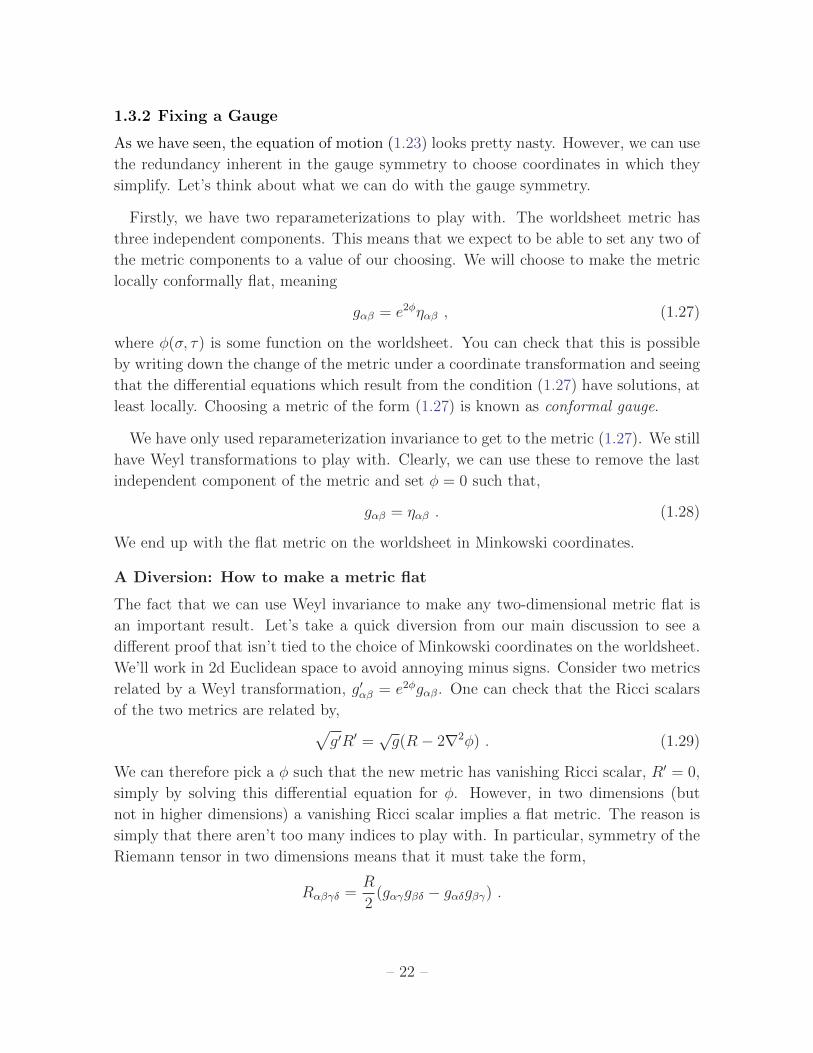
locally conformally flat, meaning

g↵� = e2�⌘↵� , (1.27)

where �(�, ⌧) is some function on the worldsheet. You can check that this is possible

by writing down the change of the metric under a coordinate transformation and seeing

that the di↵erential equations which result from the condition (1.27) have solutions, at

least locally. Choosing a metric of the form (1.27) is known as conformal gauge.

We have only used reparameterization invariance to get to the metric (1.27). We still

have Weyl transformations to play with. Clearly, we can use these to remove the last

independent component of the metric and set � = 0 such that,

g↵� = ⌘↵� . (1.28)

We end up with the flat metric on the worldsheet in Minkowski coordinates.

A Diversion: How to make a metric flat

The fact that we can use Weyl invariance to make any two-dimensional metric flat is

an important result. Let’s take a quick diversion from our main discussion to see a

di↵erent proof that isn’t tied to the choice of Minkowski coordinates on the worldsheet.

We’ll work in 2d Euclidean space to avoid annoying minus signs. Consider two metrics

related by a Weyl transformation, g0↵� = e2�g↵�. One can check that the Ricci scalars

of the two metrics are related by,pg0R0 =

pg(R� 2r2�) . (1.29)

We can therefore pick a � such that the new metric has vanishing Ricci scalar, R0 = 0,

simply by solving this di↵erential equation for �. However, in two dimensions (but

not in higher dimensions) a vanishing Ricci scalar implies a flat metric. The reason is

simply that there aren’t too many indices to play with. In particular, symmetry of the

Riemann tensor in two dimensions means that it must take the form,

R↵��� =R

2(g↵�g�� � g↵�g��) .

– 22 –

So R0 = 0 is enough to ensure that R0↵��� = 0, which means that the manifold is flat. In

equation (1.28), we’ve further used reparameterization invariance to pick coordinates

in which the flat metric is the Minkowski metric.

The equations of motion and the stress-energy tensor

With the choice of the flat metric (1.28), the Polyakov action simplifies tremendously

and becomes the theory of D free scalar fields. (In fact, this simplification happens in

any conformal gauge).

S = � 1

4⇡↵0

Zd2� @↵X · @↵X , (1.30)

and the equations of motion for Xµ reduce to the free wave equation,

@↵@↵Xµ = 0 . (1.31)

Now that looks too good to be true! Are the horrible equations (1.23) really equivalent

to a free wave equation? Well, not quite. There is something that we’ve forgotten:

we picked a choice of gauge for the metric g↵�. But we must still make sure that the

equation of motion for g↵� is satisfied. In fact, the variation of the action with respect

to the metric gives rise to a rather special quantity: it is the stress-energy tensor, T↵�.

With a particular choice of normalization convention, we define the stress-energy tensor

to be

T↵� = � 2

T

1p�g

@S

@g↵�.

We varied the Polyakov action with respect to g↵� in (1.24). When we set g↵� = ⌘↵�we get

T↵� = @↵X · @�X � 1

2

⌘↵� ⌘⇢�@⇢X · @�X . (1.32)

The equation of motion associated to the metric g↵� is simply T↵� = 0. Or, more

explicitly,

T01

= X ·X 0 = 0

T00

= T11

= 1

2

(X2 +X 0 2) = 0 . (1.33)

We therefore learn that the equations of motion of the string are the free wave equations

(1.31) subject to the two constraints (1.33) arising from the equation of motion T↵� = 0.

– 23 –

Getting a feel for the constraints

Let’s try to get some intuition for these constraints. There is a simple

Figure 8:

meaning of the first constraint in (1.33): we must choose our parame-

terization such that lines of constant � are perpendicular to the lines

of constant ⌧ , as shown in the figure.

But we can do better. To gain more physical insight, we need to make

use of the fact that we haven’t quite exhausted our gauge symmetry.

We will discuss this more in Section 2.2, but for now one can check that

there is enough remnant gauge symmetry to allow us to go to static

gauge,

X0 ⌘ t = R⌧ ,

so that (X0)0 = 0 and X0 = R, where R is a constant that is needed on dimensional

grounds. The interpretation of this constant will become clear shortly. Then, writing

Xµ = (t, ~x), the equation of motion for spatial components is the free wave equation,

~x� ~x 00 = 0

while the constraints become

~x · ~x 0 = 0

~x 2 + ~x 0 2 = R2 (1.34)

The first constraint tells us that the motion of the string must be perpendicular to the

string itself. In other words, the physical modes of the string are transverse oscillations.

There is no longitudinal mode. We’ll also see this again in Section 2.2.

From the second constraint, we can understand the meaning of the constant R: it is

related to the length of the string when ~x = 0,Zd�p(d~x/d�)2 = 2⇡R .

Of course, if we have a stretched string with ~x = 0 at one moment of time, then it won’t

stay like that for long. It will contract under its own tension. As this happens, the

second constraint equation relates the length of the string to the instantaneous velocity

of the string.

– 24 –

1.4 Mode Expansions

Let’s look at the equations of motion and constraints more closely. The equations of

motion (1.31) are easily solved. We introduce lightcone coordinates on the worldsheet,

�± = ⌧ ± � ,

in terms of which the equations of motion simply read

@+

@�Xµ = 0

The most general solution is,

Xµ(�, ⌧) = XµL(�

+) +XµR(�

�)

for arbitrary functions XµL and Xµ

R. These describe left-moving and right-moving waves

respectively. Of course the solution must still obey both the constraints (1.33) as well

as the periodicity condition,

Xµ(�, ⌧) = Xµ(� + 2⇡, ⌧) . (1.35)

The most general, periodic solution can be expanded in Fourier modes,

XµL(�

+) = 1

2

xµ + 1

2

↵0pµ �+ + i

r↵0

2

Xn 6=0

1

n↵µn e

�in�+,

XµR(�

�) = 1

2

xµ + 1

2

↵0pµ �� + i

r↵0

2

Xn 6=0

1

n↵µn e

�in��. (1.36)

This mode expansion will be very important when we come to the quantum theory.

Let’s make a few simple comments here.

• Various normalizations in this expression, such as the ↵0 and factor of 1/n have

been chosen for later convenience.

• XL and XR do not individually satisfy the periodicity condition (1.35) due to the

terms linear in �±. However, the sum of them is invariant under � ! � + 2⇡ as

required.

• The variables xµ and pµ are the position and momentum of the center of mass of

the string. This can be checked, for example, by studying the Noether currents

arising from the spacetime translation symmetry Xµ ! Xµ + cµ. One finds that

the conserved charge is indeed pµ.

• Reality of Xµ requires that the coe�cients of the Fourier modes, ↵µn and ↵µ

n, obey

↵µn = (↵µ

�n)? , ↵µ

n = (↵µ�n)

? . (1.37)

– 25 –

1.4.1 The Constraints Revisited

We still have to impose the two constraints (1.33). In the worldsheet lightcone coordi-

nates �±, these become,

(@+

X)2 = (@�X)2 = 0 . (1.38)

These equations give constraints on the momenta pµ and the Fourier modes ↵µn and ↵µ

n.

To see what these are, let’s look at

@�Xµ = @�X

µR =

↵0

2pµ +

r↵0

2

Xn 6=0

↵µn e

�in��

=

r↵0

2

Xn

↵µne

�in��

where in the second line the sum is over all n 2 Z and we have defined ↵µ0

to be

↵µ0

⌘r

↵0

2pµ .

The constraint (1.38) can then be written as

(@�X)2 =↵0

2

Xm,p

↵m · ↵p e�i(m+p)��

=↵0

2

Xm,n

↵m · ↵n�m e�in��

⌘ ↵0Xn

Ln e�in��

= 0 .

where we have defined the sum of oscillator modes,

Ln =1

2

Xm

↵n�m · ↵m . (1.39)

We can also do the same for the left-moving modes, where we again define an analogous

sum of operator modes,

Ln =1

2

Xm

↵n�m · ↵m . (1.40)

with the zero mode defined to be,

↵µ0

⌘r

↵0

2pµ .

– 26 –

The fact that ↵µ0

= ↵µ0

looks innocuous but is a key point to remember when we come

to quantize the string. The Ln and Ln are the Fourier modes of the constraints. Any

classical solution of the string of the form (1.36) must further obey the infinite number

of constraints,

Ln = Ln = 0 n 2 Z .

We’ll meet these objects Ln and Ln again in a more general context when we come to

discuss conformal field theory.

The constraints arising from L0

and L0

have a rather special interpretation. This is

because they include the square of the spacetime momentum pµ. But, the square of the

spacetime momentum is an important quantity in Minkowski space: it is the square of

the rest mass of a particle,

pµpµ = �M2 .

So the L0

and L0

constraints tell us the e↵ective mass of a string in terms of the excited

oscillator modes, namely

M2 =4

↵0

Xn>0

↵n · ↵�n =4

↵0

Xn>0

↵n · ↵�n (1.41)

Because both ↵µ0

and ↵µ0

are equal top↵0/2 pµ, we have two expressions for the invariant

mass: one in terms of right-moving oscillators ↵µn and one in terms of left-moving

oscillators ↵µn. And these two terms must be equal to each other. This is known as

level matching. It will play an important role in the next section where we turn to the

quantum theory.

– 27 –