Strong Coupling Theory of Magic-Angle Graphene: A

Pedagogical Introduction

Patrick J. Ledwith, Eslam Khalaf, Ashvin Vishwanath

Harvard University, Cambridge, MA 02138, USA.

May 13, 2021

Abstract

We give a self contained review of a recently developed strong coupling theory of magic-anglegraphene. An advantage of this approach is that a single formulation can capture both theinsulating and superconducting states, and with a few simplifying assumptions, can be treatedanalytically. We begin by reviewing the electronic structure of magic angle graphene’s flat bands,in a limit that exposes their peculiar band topology and geometry. We highlight how similaritiesbetween the flat bands and the lowest Landau level give insight into the effect of interactions. Forexample, at certain fractional fillings, we note the promise for realizing fractional Chern states.At integer fillings, this approach points to flavor ordered insulators, which can be captured by asigma-model in its ordered phase. Unexpectedly, topological textures of the sigma model carryelectric charge which allows us to extend the same theory to describe the doped phases awayfrom integer filling. We show how this approach can lead to superconductivity on disorderingthe sigma model, and estimate the Tc for the superconductor. We highlight the importantrole played by an effective super-exchange coupling both in pairing and in setting the effectivemass of Cooper pairs. Seeking to enhance this coupling helps predict new superconductingplatforms, including the recently discovered alternating twist trilayer platform. We also contrastour proposal from strong coupling theories for other superconductors.

0 Introduction

In early 2018, the experimental discovery of a host of novel phenomena in twisted bilayergraphene (TBG) took the physics world by storm [1, 2]. New insulating states induced byelectron-electron interactions, as well as robust superconducting states were discovered. Theseexperiments built on earlier work [3, 4, 5, 6, 7, 8, 9, 10, 11, 12, 13] that pointed to the exis-tence of exceptionally narrow and isolated bands arising from the moire pattern obtained ontwisting the two graphene sheets close to a ‘magic angle’, i.e. magic angle TBG (MATBG).The condensed matter community had perhaps not witnessed such a tectonic shift since theexperimental discovery of high temperature superconductivity, more than three decades earlier.

There were other parallels between the two discoveries. Although MATBG with a super-conducting transition temperature of a few Kelvin may seem like an unlikely candidate for thetitle of a high Tc superconductor, a proper comparison of scales is required. At the magic angleof 1.1 degree (θ 1/50th of a radian), many relevant scales - from the lattice spacing to the sizeof the Coulomb interaction - are scaled by this small angle. Thus, a better comparison withthe cuprates or other correlated solids, is obtained by scaling Tc by the small angle (expressed

in radian) Tc/θ, which yields values consistent with the high Tc family. Additionally, in bothcases, interacting insulating states and superconductors appear in conjunction in typical phasediagrams and strange metal transport has been reported on raising temperature (see eg. ref [14]for a review).

At the same time, there are several important distinctions. A principle distinction that willbe emphasized here is the nontrivial quantum band geometry of the flat bands of MATBG.This is a special feature arising from graphene’s Dirac electrons. On the experimental side, themost striking manifestation of this feature is the emergence of spontaneous integer quantumHall states (anomalous quantum Hall) under certain conditions in twisted bilayer systems. Thisremarkable unification of quantum Hall and high Tc superconductivity in a single experimentalplatform, points to this underlying unique feature of TBG.

In 1987, shortly after the discovery of the cuprate high temperature superconductors, An-derson [15] published a short paper ”The Resonating Valence Bond (RVB) Theory of Supercon-ductivity” where he outlined the foundations of a theoretical program for the cuprates. Alongwith several other key ideas, it was proposed that (i) the underlying model was the HubbardModel with hopping t and onsite Coulomb repulsion U that would give rise to local magneticmoments with an antiferromagnetic coupling J ∼ t2/U (super-exchange) between them and (ii)the seeds of superconductivity were already contained in the insulator and charge doping simplyreleased the singlets created by the superexchange, which then condensed into the supercon-ducting state. Consequently, at low doping the superconducting Tc was predicted to be limitedby phase fluctuations. Notwithstanding the fact that later experiments have painted a rich andcomplex picture of the cuprates, these seminal ideas made a deep impression that lasts to thisday.

Translating this program into one that applies to MATBG, immediately runs into problems.As was noticed starting very early on [16, 17, 18, 19], writing down a tight binding model thatcaptures the flat bands alone, while preserving all relevant symmetries, runs into a topologicalobstruction. One must ether give up on some symmetries, such as the 180 degree rotationsymmetry C2z or conservation of valley charge (valley U(1)) [20] or augment the model withadditional bands [21, 16, 17]. Note, preserving these symmetries is not simply a technical nicety- they are the precise symmetries responsible for the band touching of the two bands of magicangle graphene. What then plays the role of the underlying physical model, analogous to theHubbard model employed for the cuprates?

In the first section of this review we outline an approach to studying the single particleeigenstates directly in momentum space and advocating for a choice of basis that will make thesubsequent discussion, on including interaction effects, natural. This is made explicit by tuningto a particular ‘chiral limit’, where the model has remarkably simple features. In fact on tuningangle, perfectly flat bands are obtained, and even the form of the single particle wavefunctionsin this limit can be derived (almost entirely) from analytic arguments[22]. A close analogyto quantum Hall wavefunctions is pointed out; this model has several attractive mathematicalfeatures that remain to be fully understood [23, 24, 25, 26, 27]. The central observation hereis that one can make linear combination of bands that are simulataneously both sublatticepolarized and carry unit Chern number. This property holds even away from the chiral limitand forms the starting point for a strong coupling theory of integer filling in Section 2.

The strong coupling theory, when applied to integer fillings, predicts insulating states whichcan be thought of as generalized flavor ferromagnets. In all, there are eight nearly flat bands.A fourfold degeneracy is attributed to spin and valley. In addition a further twofold banddegeneracy is present, corresponding roughly to the two sublattices of graphene. We show howin an idealized limit a flavor ferromagnet is predicted, and a large emergent symmetry relatesvarious flavor orders. On moving away from the ideal limit, , various anisotropies emerge thatselect a subset of flavor ordered ground states. The ground state is thus a relatively conventionalstate, well approximated by Hartree Fock wavefunctions, and is to be contrasted with the exoticinsulator proposed by Anderson for the cuprates, an RVB quantum spin liquid [15]. However,in one respect they do fit within the Anderson viewpoint. Somewhat to our surprise [28], it wasfound that doping the insulators did not require adding any additional charge degrees of freedom.

2

Instead, charge excitations in the form of skyrmions were already present in the model. Further,it was realized that in certain cases these were nothing but Cooper pairs which can condense,leading to an all electronic mechanism for superconductivity. The transition temperature forthis mechanism is calculated in a simplified limit and the results are broadly in agreement withexperimental data in the low doping limit. Numerical DMRG simulations that capture essentialfeatures of this model reveal that indeed the presence of low energy skyrmion excitations nearinteger filling is closely tied to the appearance of superconductivity at finite doping [29]. Thisis the subject of Section 3. In addition to this detailed mechanism, a more basic feature isthe presence of a superexchange interaction between opposite Chern sectors, which plays animportant role in pairing.

Let us further contrast the mechanism outlined above with the RVB idea, by placing bothin a broader context. We note that in the modern parlance the RVB state has topologicalorder and fractionalization in the precise sense that it has emergent excitations with unusualstatistics and quantum numbers. This obviously goes beyond the idea of classical Landauorder parameters. In contrast the insulators we propose for TBG are flavor ordered phases,without fractionalization. However, thanks to the nontrivial bands of magic angle graphene,these orders are not entirely classical - for instance topological textures such as skyrmions carryelectric charge. Such spontaneous symmetry breaking in topological bands have previouslybeen discussed in relation to superconductivity [30, 31], however a microscopic realization ofthe relevant type of insulator itself has proved elusive. Here we explain how the flavor orderedstates of MATBG at even integer filling fulfill these requirements.

Naturally, predictions for new platforms for superconductivity should emerge from a deeperunderstanding of the physical mechanism. For cuprate superconductors, once key ingredientswere identified, a class of nickelate materials were deemed promising analogs and have recentlybeen fabricated and shown to exhibit superconductivity [32]. In the strong coupling approachto MATBG described here, the principle goal is to enhance a superexchange coupling J , whichin the typical settings of graphene moire systems is related to C2 symmetric structures. Whilethere is already a vast library of graphene based moire materials, MATBG is one of the fewthat exhibits this symmetry. Alignment with a substrate of hBN for example leads to symmetrylowering. A rare class of structures which have all the requisite ingredients for the strongcoupling mechanism described above are the alternating twist multilayers [33]. This is thesubject of Section 4, including both trilayer and tetralayer, the first of which were recentlyreported in experiment to possess robust superconductivity.

1 Single Particle Electronic Structure

In this section we describe how to go from two decoupled graphene sheets to the topologicalflat bands of twisted bilayer graphene. We start from the low energy graphene Dirac conesin each layer and couple them through tunneling between layers. This tunneling has a moireperiodicity that is reflected in the twisted bilayer graphene band structure. Finally, we describea ”chiral” limit where tunneling at AA stacking sites is neglected. In this limit we find that thewavefunctions are very similar to those of the lowest Landau level (LLL). This structure of thewavefunctions has implications for the possibility of fractional Chern insulating (FCI) states intwisted bilayer graphene. It also sets the stage for treating interactions at integer filling.

To set notation, let us begin with the electronic structure of graphene. It consists of two bandsthat cross at two Dirac cones at the K and K ′ points in the Brillouin zone (BZ). There is oneelectron per unit cell, and so accounting for spin we should fill up the bottom band. The lowenergy dispersion thus consists of the Dirac cones

H = vF(px σx ⊗ τ0 + py σy ⊗ τz

)(1)

3

where σz. = ±1 corresponds to the A, B sublattices of graphene and τz = ±1 correspondsto the K, K ′ valleys of graphene.

Now consider the twisted bilayer in the continuum limit, focusing on a single valley; we willderive the Bistritzer-Macdonald (BM) Hamiltonian [8]. We can write the Hamiltonian in thetwo layers as:

H+ =

[HUU HUD

HDU HDD

](2)

We begin with independent layers and then couple them together. The Up and Down layerDirac Hamiltonians are:

HUU = vF (−i∇−KU) · σθ/2HDD = vF (−i∇−KD) · σ−θ/2

(3)

where we have taken into account the shift of the Dirac points and the Pauli matrices due torotation so that σθ/2 = e−i

θ4σz (σx, σy)e+i θ4σz . We now couple the Dirac points together by

interlayer hopping terms HDU = H†UD where :

HUD = T0(r)σ0 + TAB(r)σ+ + TBA(r)σ− (4)

Let us now derive the form of the tunneling matrix elements - for better intuition first considervery local tunneling (i.e. electrons tunnel only when the atoms of the two layers occlude eachother). We then need to consider three cases, where (i) the atoms of both sublattices are on topof each other, the so called AA or equivalently the BB regions which form a triangular lattice,see Figure 1; (ii) where the A atoms of the lower layer align with the B atoms of the upper layer(AB regions), they form one sublattice of a honeycomb lattice on the moire scale; and finally(iii) the BA regions, where B atoms of the lower layer align with the A atoms of the upper layerand form the other sublattice of the honeycomb lattice on the moire scale.

Tunneling, say in the AA regions, could be represented as: T0 ∼∑n δ(r−Rn) where the sum

runs over the triangular moire lattice sites locations. From the Poisson resummation formula thiscan be equivalently written as

∑n δ(r−Rn) = 1

AM

∑m e−iGm·r, where AM is the area of the

moire unit cell and Gm are the moire lattice reciprocal vectors. On the other hand the tunnelingmatrix elements in the other regions acquire additional phase factors due to their displacementfrom the unit cell centers. They are TAB ∼

∑n δ(r−Rn − rA) = 1

AM

∑m e

iGm·rAe−iGm·r and

TBA ∼∑n δ(r−Rn − rB) = 1

AM

∑m e

iGm·rBe−iGm·r. In reality, one has to take into account

a more general interlayer hopping T (r) with Fourier components T (Gm). Since the interlayerhopping depends on the 3D separation between atoms, and the separation between layers is morethan twice the intra-layer atomic separations, we expect the Fourier components to decreaserapidly and we can keep the lowest order harmonics [34]. To obtain the tunneling strengths forthe lowest order harmonics we will appeal to rotation symmetry. Note the original choice ofKU/D for the Dirac points breaks rotation symmetry. To make rotation symmetry manifest, wewill move the Dirac points in both layers to the origin using the unitary transformation with

diagonal entries: W = eiKU·r, eiK

D·r. This leads to the following transformed Hamiltonian:

H ′UU = vF (−i∇) · σθ/2H ′DD = vF (−i∇) · σ−θ/2

(5)

We define bq1 = KU −KD = kθ(0,−1), and the vectors related by 2π/3 rotations q2,3 =

kθ(±√

3/2, 1/2). Then we can write the tunneling matrix elements as

H ′UD = w0U0(r)σ0 + w1UAB(r)σ+ + w1UBA(r)σ− (6)

U0(r) = e−iq1·r + e−iq2·r + e−iq3·r

UAB(r) = e−iq1·r + ei2π3 e−iq2·r + ei

4π3 e−iq3·r

UBA(r) = e−iq1·r + e−i2π3 e−iq2·r + e−i

4π3 e−iq3·r

(7)

4

The BM Hamiltonian has the translation symmetry

H(r + a1,2) = V H(r)V † V = diag(1, e−iφ, 1, e−iφ), (8)

where the moire lattice vectors a1,2 and reciprocal lattice vectors b1,2 are

a1,2 =4π

3kθ

(±√

3

2,

1

2

), b1,2 = q2,3 − q1 = kθ

(±√

3

2,

3

2

). (9)

We will find it useful to sometimes use triangular lattice and reciprocal lattice coordinates

ri =r · bi2π

ki =k · ai

2π(10)

which satisfy r = r1a1 + r2a2 and k = k1b1 + k2b2.The relative phase shift between the top and bottom layers under translations in (8) can

be understood from the misalignment of their graphene Brillouin zones due to the twist angleθ. In particular, momenta in the bottom layer are shifted by q1 relative to the top layer whichgenerates the phase shift eiq1·a1,2 = e−iφ under translations. This is encoded in the form of theBloch states

ψk(r) = uk(r)

(ei(k−K)·r

ei(k−K′)·r

), (11)

where K ′ = K−q1 is the moire K ′ point wavevector in terms of the moire K point wavevector.For zero tunneling, or large angles, the states at K (K ′) correspond to the top layer and bottomgraphene layer respectively.

Note, in the simplest approximation w0 = w1 ∼ 110meV . However, later work [35, 21]showed that inter layer relaxation, relaxation followed by intra-layer relaxation reduce the ratioκ = w0/w1 from unity to κ = 0.8 and further κ = 0.75. This quantity will play an importantrole and we will often treat it as a free parameter.

1.1 The Chiral Model: A simple limiting case

It will be particularly interesting to consider the chiral limit, where κ = 0. As we show in thissection, in this limit, there exists an exactly flat zero energy flat band [22]. Furthermore, thewavefunctions are very similar to those of the LLL; they have identical quantum geometry in asense that we will make precise. This result implies that we can expect chiral twisted bilayergraphene to host fractional Chern insulator ground states, at least for a sufficiently short rangeinteraction potential [36].

We begin with the Bistritzer-Macdonald (BM) model discussed above

H =

(−ivσθ/2 ·∇ T (r)

T †(r) −ivσ−θ/2 ·∇

)(12)

with

T (r) =

(w0U0(r) w1U1(r)w1U

∗1 (−r) w0U0(r)

),

U0(r) = e−iq1·r + e−iq2·r + e−iq3·r,

U1(r) = e−iq1·r + eiφe−iq2·r + e−iφe−iq3·r,

(13)

The vectors qi are q1 = kθ(0,−1) and q2,3 = kθ(±√

3/2, 1/2) and φ = 2π/3.For the following discussion we choose units where v = kθ = 1. We will also find it useful

to choose the origin of the moire BZ to be the K point to simplify some later expressions, eventhough the most symmetric choice is the Γ point.

A very useful appproximation to the above Hamiltonian is to set κ = 0, such that tunnellingonly occurs in AB regions. Realistically we expect κ ≈ 0.7 < 1 due to relaxation effects. While

5

decreasing it all the way to zero is a drastic approximation, we will find it useful to do so atfirst and then examine the effects of going back to a realistic value of κ later in these notes. Themodel with κ = 0 is known as the chiral model because it has the chiral symmetry σzHσz = −H.That is, given an eigenstate |Ψ〉 of H with energy E, one can generate an eigensate σz|Ψ〉, aneigenstate with energy −E. Further, zero energy eigenstates can be chosen to be eigenstates ofσz, i.e. they are sublattice polarized. Below, we will show the existence of special (magic) angleswhere the entire band is at zero energy. As a consequence we can define a sublattice polarizedbasis for these eigenstates. What is less obvious is that these sublattice polarized bands alsocarry Chern number of one [22, 37], and in fact share many similarities, in ways that will bemade precise below, with the LLL[36].

The chiral symmmetry is especially useful at the magic angle; here we obtain exactly flatbands at zero energy that are eigenstates of σz. Since we are interested in zero modes that areeigenstates of σz, we rewrite the Hamiltonian by exchanging the second and third columns afterwhich σz = diag(1, 1,−1,−1) and

H =

(0 D†

D 0

)D =

(−2i∂ αU1(r)

αU1(−r) −2i∂

), (14)

with α = w1 = w1/vkθ. Because H,σz = 0, zero energy solutions may be chosen to beeigenstates of σz. We therefore search for solutions to the equation Dψk(r) = 0 for each moireBloch momentum k. The solutions when σz = −1 can be obtained using C2T symmetry:χk(r) = ψ∗k(−r).

1.1.1 Zero Modes of Chiral Model:

When k = K, we are guaranteed a zero mode solution by continuity from α = 0, i.e. the

unperturbed Dirac points in the two layers. This is because the zero mode ψK =(1 0

)Tis

pinned to zero energy because it is an eigenstate of σz and it cannot move to different values ofk because it is pinned to k = K by C3 symmetry. Thus ψK has zero energy for all α > 0.

Next we note that becauseD only has antiholomorphic derivativesD (F (z)ψK(r)) = F (z)DψK(r) =0 for any holomorphic function F (z) where z = x+ iy. However, any holomorphic function F (z)is either constant or blows up at infinity by Liouville’s theorem. Hence, this state cannot be aBloch state at a momentum other than K. At this point it may appear that we cannot obtainzero modes except at isolated crystal momenta. However there is way out - we can allow F (z)to be a meromorphic function. Although such a function would necessarily have poles at cer-tain positions in the unit cell, we could arrange for them to be precisely cancelled by zeros inψK(r). Note, since this is a spinor wavefunction, we will need both components of ψK(r) tosimultaneously vanish at that location in the unit cell. We can explore if such a condition issatisfied by varying the angle. Indeed the magic angles are precisely those angles for which ψKhas a zero in both of its components at some r.

In fact, symmetry helps us locate where the zero will appear. We focus on the points ±r0, theBA/AB stacking points respectively with r0 = 1

3 (a1 − a2) = 0. These points are distinguishedby C3 symmetry since they map to themselves up to a lattice vector, C3r0 = r0 +a2, see Fig.1.We show that three fold rotation symmetry implies that one of the components ψK2(±r0) = 0.Indeed, C3 symmetry implies ψK(Rφr) = ψK(r) where Rφ rotates vectors by an angle φ. Onemay deduce that this is the correct representation by continuity from α = 0 where ψK = (1, 0)T .However, we additionally have

ψK2(±r0) = ψK2(±Rφr0) = ψK2(±r0 ± a2) = e∓iφψK2(±r0) (15)

since due to the form of the Bloch states (8) the second component of ψK picks up a phaseunder translations.

While it is possible to show that DψK = 0 does not allow for ψK1(−r0) = 0, it is possiblefor the single component ψK1(r0) = 0 (which can be chosen real) by tuning the angle. Thus wehave one tuning parameter to set a single real number to zero, which generically will give a series

6

Figure 1: Real space visualization of the moire pattern and depiction of the AA stacking r = 0,AB stacking r = −r0, and BA stacking r = r0 points. All three of these points map to themselvesup to shifts by lattice vectors under C3 symmetry

of points as solutions, i.e. magic angles. The first of these angles is at nearly the same angle asrealistic TBG and can be approximated using perturbation theory for small α. In particular,we plug in the ansatz

ψK =

(1 + α2u2 + · · ·αu1 + · · ·

)(16)

to the zero mode equation DψK = 0 and obtain

u1 = −i(eiq1·r + eiq1·r + eiq1·r) u2 =i√3e−iφ(e−ib1·r + eib2·r + ei(b1−b2)·r) + c.c. (17)

We then compute u1(r0) = 0 and u2(r0) = −3 such that when α ≈ 1/√

3 ≈ 0.577 the entirespinor vanishes. The perturbation expansion may be carried out to higher orders and seems toget arbitrarily close to the numerically obtained value of α1 ≈ 0.586 for the first chiral magicangle. There seem to be infinitely many α for which ψK vanishes with the quasiperiodicityαn ≈ αn−1+1.5 holding for large α. Other metrics such as vanishing of Dirac velocity, maximumgap to neighboring bands and minimum bandwidth also gives the same result. See ref. [22] formore details.

1.1.2 Wavefunctions and topology:

To generate the rest of the states in the band we need to choose a meromorphic functionFk(z) that is Bloch periodic. To do so, we write Fk(z) = fk(z)/g(z) where both fk and g areholomorphic and g(z0 +ma1 +na2) = 0 where z0 = r0x+ ir0y and similarly a1,2 are the complexnumber versions of the lattice vectors a1,2. The only choice for g(z), up to multiplication by anexponential function, is the Jacobi theta function.

g(z) = ϑ1

(z − z0

a1

∣∣∣∣ω) , ϑ(u|τ) = −i∞∑

n=−∞(−1)neπiτ(n+ 1

2 )2+πi(2n+1)u, (18)

7

where ω = eiφ. Under translations the Jacobi theta function satisfies

ϑ1(u+ 1|τ) = −ϑ1(u|τ), ϑ1(u+ τ |τ) = −e−πiτ−2πiuϑ1(u|τ). (19)

and ϑ1(0|τ) = 0 such that g(z) has the desired zeros (note that a translation by a1 shifts ar-gument of the theta function by 1 while a translation by a2 shifts the argument of the thetafunction by a2/a1 = eiφ = τ). The properties (19) enable us to construct Bloch states by choos-ing fk(z) to also be a theta function, since although a single theta function is only an eigenstateunder translations in one direction, the above u dependence in translations proportional to τwill always cancel out in any ratio of theta functions leaving a pure phase. This pure phase maybe manipulated by shifting the arguments of the theta functions relative to each other, and anexponential function can also be included as an additional knob. We may therefore engineerfk(z) = e2πik1z/a1ϑ1((z − z0)/a1 − k/b2|ω) for k = kx + iky (measured from the K point) suchthat

ψk(r) = e2πik1z/a1ϑ1

(z − z0

a1− k

b2

∣∣∣∣ω) ψK(r)

ϑ1

(z−z0a1|ω) ,

uk(r) = e−ik·rψbk(r) = e−2πir2k/b2ϑ1

(z − z0

a1− k

b2

∣∣∣∣ω) uK(r)

ϑ1

(z−z0a1|ω) , (20)

are Bloch periodic and periodic under translations respectively.Let us make two observations - first, note the functional dependence of Bloch wavefunctions

uk(r) on moving through the BZ. In the gauge we have chosen, the entire dependence is viak = kx + iky, i.e. it is an analytic function of k. Next, note that these wavefunctions describe aChern band with C = +1. To see this, we note that uk(r) is well defined for all k and r withno singularities, but it is not periodic under k 7→ k + b1,2. Instead, using (19) we have

uk+b1(r) = −e−2πir1eiπω+2πiz0e2πik/b2uk(r),

uk+b2(r) = −e−2πir2uk(r)

(21)

For the Berry connection A(k) = −i 〈uk|∇k |uk〉, where u = u/‖u‖ is a normalized wavefunc-tion, this implies

A(k + b1) = A(k) +1

2a1 + a2, A(k + b2) = A(k) (22)

For both (21) and (22) we used b1/b2 = −ω, and for (22) we used triangular lattice coordinateswhere 2π∇k = a1∂k1 + a2∂k2 . The Chern number can be evaluated as

2πC =

∫BZ

∇×A =

∮∂BZ

A · dk

=

∫ 1

0

(A(k1b1)−A(k1b1 + b2)) · b1dk1 +

∫ 1

0

(A(b1 + k2b2)−A(k2b2)) · b2dk2

= a2 · b2 = 2π,

(23)

and so C = 1. The C2T related band with σz = −1 then has C = −1. Including the bands fromthe other graphene valley and spin degeneracy, we obtain four exactly flat bands with C = +1and four exactly flat bands with C = −1.

Such a situation seems extremely close to that of quantum Hall ferromagnetism with twoimportant differences. The first is that there is an extra time reversed copy with opposite Chernnumbers. The second is that these flat bands are not precisely the same as the LLL. How canwe understand and quantify the latter distinction? The coarse indicators of flat dispersion andChern number are the same.

Before we answer this question, we make a side comment on how κ > 0 affects the bands.Because chiral symmetry is no longer present, there is no longer a basis where the wavefunctions

8

(b)

<latexit sha1_base64="BawSIn5+SNlhF960ZUcF5h2S7jk=">AAAB73icbVDLSgNBEOyNrxhfUY9eBoMQL2FXInoMevEYwTwgCWF20psMmZ1dZ2aFsOQnvHhQxKu/482/cZLsQRMLGoqqbrq7/FhwbVz328mtrW9sbuW3Czu7e/sHxcOjpo4SxbDBIhGptk81Ci6xYbgR2I4V0tAX2PLHtzO/9YRK80g+mEmMvZAOJQ84o8ZK7a4fpGX/fNovltyKOwdZJV5GSpCh3i9+dQcRS0KUhgmqdcdzY9NLqTKcCZwWuonGmLIxHWLHUklD1L10fu+UnFllQIJI2ZKGzNXfEykNtZ6Evu0MqRnpZW8m/ud1EhNc91Iu48SgZItFQSKIicjseTLgCpkRE0soU9zeStiIKsqMjahgQ/CWX14lzYuKV61c3ldLtZssjjycwCmUwYMrqMEd1KEBDAQ8wyu8OY/Oi/PufCxac042cwx/4Hz+AIF9j6E=</latexit>

(a)

<latexit sha1_base64="8ghNgIcNJqScW2x7tWV5cZR9u1A=">AAAB73icbVDLSgNBEOyNrxhfUY9eBoMQL2FXInoMevEYwTwgCWF2MpsMmZ1dZ3qFsOQnvHhQxKu/482/cZLsQRMLGoqqbrq7/FgKg6777eTW1jc2t/LbhZ3dvf2D4uFR00SJZrzBIhnptk8Nl0LxBgqUvB1rTkNf8pY/vp35rSeujYjUA05i3gvpUIlAMIpWanf9IC3T82m/WHIr7hxklXgZKUGGer/41R1ELAm5QiapMR3PjbGXUo2CST4tdBPDY8rGdMg7lioactNL5/dOyZlVBiSItC2FZK7+nkhpaMwk9G1nSHFklr2Z+J/XSTC47qVCxQlyxRaLgkQSjMjseTIQmjOUE0so08LeStiIasrQRlSwIXjLL6+S5kXFq1Yu76ul2k0WRx5O4BTK4MEV1OAO6tAABhKe4RXenEfnxXl3PhatOSebOYY/cD5/AH/3j6A=</latexit>

(c)

<latexit sha1_base64="vQ7X+KgyaC9zSOwyv8vHN9Dv9yE=">AAAB73icbVDLSgNBEOyNrxhfUY9eBoMQL2FXInoMevEYwTwgCWF2MpsMmZ1dZ3qFsOQnvHhQxKu/482/cZLsQRMLGoqqbrq7/FgKg6777eTW1jc2t/LbhZ3dvf2D4uFR00SJZrzBIhnptk8Nl0LxBgqUvB1rTkNf8pY/vp35rSeujYjUA05i3gvpUIlAMIpWanf9IC2z82m/WHIr7hxklXgZKUGGer/41R1ELAm5QiapMR3PjbGXUo2CST4tdBPDY8rGdMg7lioactNL5/dOyZlVBiSItC2FZK7+nkhpaMwk9G1nSHFklr2Z+J/XSTC47qVCxQlyxRaLgkQSjMjseTIQmjOUE0so08LeStiIasrQRlSwIXjLL6+S5kXFq1Yu76ul2k0WRx5O4BTK4MEV1OAO6tAABhKe4RXenEfnxXl3PhatOSebOYY/cD5/AIMDj6I=</latexit>

(d)

<latexit sha1_base64="/iBJUin0DzszpXFWN6e22vcjyiY=">AAAB73icbVBNSwMxEJ2tX7V+VT16CRahXsquVPRY9OKxgv2AdinZbLYNzSZrkhXK0j/hxYMiXv073vw3pu0etPXBwOO9GWbmBQln2rjut1NYW9/Y3Cpul3Z29/YPyodHbS1TRWiLSC5VN8CaciZoyzDDaTdRFMcBp51gfDvzO09UaSbFg5kk1I/xULCIEWys1O0HUVYNz6eDcsWtuXOgVeLlpAI5moPyVz+UJI2pMIRjrXuemxg/w8owwum01E81TTAZ4yHtWSpwTLWfze+dojOrhCiSypYwaK7+nshwrPUkDmxnjM1IL3sz8T+vl5ro2s+YSFJDBVksilKOjESz51HIFCWGTyzBRDF7KyIjrDAxNqKSDcFbfnmVtC9qXr12eV+vNG7yOIpwAqdQBQ+uoAF30IQWEODwDK/w5jw6L86787FoLTj5zDH8gfP5A4SJj6M=</latexit>

(e)

<latexit sha1_base64="SK737FeeZ11NRMwaANMe2LqmEjI=">AAAB73icbVDLSgNBEOyNrxhfUY9eBoMQL2FXInoMevEYwTwgCWF20psMmZ1dZ2aFsOQnvHhQxKu/482/cZLsQRMLGoqqbrq7/FhwbVz328mtrW9sbuW3Czu7e/sHxcOjpo4SxbDBIhGptk81Ci6xYbgR2I4V0tAX2PLHtzO/9YRK80g+mEmMvZAOJQ84o8ZK7a4fpGU8n/aLJbfizkFWiZeREmSo94tf3UHEkhClYYJq3fHc2PRSqgxnAqeFbqIxpmxMh9ixVNIQdS+d3zslZ1YZkCBStqQhc/X3REpDrSehbztDakZ62ZuJ/3mdxATXvZTLODEo2WJRkAhiIjJ7ngy4QmbExBLKFLe3EjaiijJjIyrYELzll1dJ86LiVSuX99VS7SaLIw8ncApl8OAKanAHdWgAAwHP8ApvzqPz4rw7H4vWnJPNHMMfOJ8/hg+PpA==</latexit>

Figure 2: Berry curvature [36] for the σz = +1 band of magic angle graphene for different valuesof κ. Panels (a)− (e) have κ = 0, 0.2, 0.4, 0.6, 0.8 respectively.

are completely sublattice polarized. However, one may choose the basis where the sublatticeoperator Γab(k) = 〈uak|σz |ubk〉 is diagonal. The two bands are exchanged by C2T as be-fore. Furthermore, C2T symmetry implies that in this basis the non-Abelian Berry connectionAab(k) = 〈uak|∇k |ubk〉 is diagonal, We may therefore continue to use sublattice σz = ±1 tolabel the two bands, and the two bands continue to have opposite Chern numbers in this basis.The Berry curvature of the σz = +1 band is shown in Figure 2 for various values of κ. Atlarge κ there is a sharp increase in the Berry curvature at the Γ point due to approaching bandcrossings with the remote bands.

1.1.3 Quantum Geometry of the Chiral Flat Bands:

To understand the similarities and differences between the chiral flat TBG bands and Landaulevels we review how to characterize the geometry of a band. We begin by considering the Blochoverlaps, or form factors, 〈uk1

|uk2〉 that appear in any physical quantity that is indifferent to

the “internal” indices of the wavefunctions: in the case of chiral TBG, this is layer and theposition r within a unit cell. There are two important aspects of these overlaps: their phaseand magnitude. The bare phase is not gauge invariant, but if we consider the phase of an overlapthat traces a small loop in k-space we obtain a gauge invariant quantity from which we mayextract the Berry curvature:

Ω(k) = limq→0

q−2 ImP(k)

P (k) =⟨uk− qx2 −

qy2

∣∣∣uk+ qx2 −

qy2

⟩⟨uk+ qx

2 −qy2

∣∣∣uk+ qx2 + qy

2

⟩⟨uk+ qx

2 + qy2

∣∣∣uk− qx2 + qy2

⟩⟨uk− qx2 + qy

2

∣∣∣uk− qx2 − qy2 ⟩(24)

However, Berry curvature is not sufficient to describe band geometry on its own. For example,all Landau levels with constant magnetic field have the same Berry curvature Ω = `2B but theyhave very different band geometry with important implications: charge density waves become theground state at fractional Landau level filling after the first few Landau levels. The origin of thisdifference is that there is information contained in the magnitude of the Bloch overlaps as well

9

that the Berry curvature does not take into account. The variation in magnitude correspondsto the quantum distance between k-points and associated Fubini-Study metric

D(k1,k2) = 1− |〈uk1 |uk2〉|, gab(k) =∂

∂qa

∂

∂qbD(k,k + q)

∣∣q=0

. (25)

For the n’th Landau level, where zero is the lowest, the Fubini study metric is

gab(k) =

(n+

1

2

)`2Bδab. (26)

The increase relative to the LLL comes from the Laguerre polynomial in the form factor|〈uk|uk+q〉| = Ln(q2`2B/2) exp

(−q2`2B/4

). The node in the form factor due to the Laguerre

polynomial helps stabilize charge density wave states in higher Landau levels [38].The Berry curvature and Fubini-Study metric are tied together in special systems. One may

see this by constructing a gauge invariant complex tensor sometimes referred to as the “quantummetric” which is schematically written as η = g−2iεΩ, where g is the symmetric F-S metric andε is the antisymmetric matrix. This can be compactly written in terms of the gauge invariantprojector Q(k) as:

ηab(k) =〈∂kauk|Q(k) |∂kbuk〉

〈uk|uk〉, Q(k) = 1− |uk〉 〈uk|

〈uk|uk〉. (27)

The quantum metric is Hermitian and positive semidefinite because it proportional to a pro-jection of Q(k) onto the subspace spanned by the states |∂kxuk〉 and

∣∣∂kyuk⟩, and Q(k) ismanifestly Hermitian and positive semidefinite as a projection operator. The real and imagi-nary components of η can be seen to correspond to the Fubini Study metric and Berry curvaturerespectively

Ω = −1

2Im ηxy =

1

2Im ηyx, gab = Re ηab (28)

and the fact that η is positive semidefinite, det η ≥ 0, implies that det g(k) ≥ |Ω(k)|2/4. Theinequality is saturated for all two band systems, as well as other special systems. A strongercondition that very few systems satisfy is obtained if we additionally require that the eigenvectorsof g(k) are the same for all k. This is not implied by any rotation symmetry, as the rotationsymmetry changes the value of k. In this case, we may simultaneously diagonalize g(k) at allvalues of k and obtain

gab(k) =1

2|Ω(k)|δab, tr g(k) = |Ω(k)| (29)

This saturates the inequality tr g ≥ |Ω(k)| which may be derived from the determinantinequality above. The trace condition (29) is much harder to satisfy than the analogous deter-minant condition. We will soon show that (29) is satisfied exactly by the lowest Landau level(which further satisfies Ω(k) independent of k) as well as chiral TBG. It is strongly violated forall higher Landau levels. Such a distinction is important because the physics of higher Landaulevels is very different from the lowest Landau level, even though all Landau levels are flat andhave identical Berry curvature and Chern number. In particular, most fractional quantum Hallstates are observed in the lowest Landau level, and none are observed for the second and higherLandau levels.

Notably, if the Bloch states |uk〉 can be chosen to be holomorphic in k = kx+iky, then (29) issatisfied. The reason can be seen directly from (27) upon replacing ∂kxuk = (∂k+∂k)uk = ∂kukand similarly ∂kyuk = i∂kuk. We then obtain

η(k) ∝(

1 i−i 1

)(30)

from which (29) follows. This is the reason why the LLL Bloch states satisfy (29), and in thatcase continuous magnetic translation symmetry additionally implies that Ω(k) is independentof k.

10

Figure 3: Flowchart for results of importance to FCI physics. Both the chiral TBG flat band andDirac LLL (for a possibly inhomogeneous magnetic field) are zero modes of an operator that onlycontains antiholomorphic derivatives. The real space dependence of the Bloch states thus has aholomorphic factor which may be used to write fractional quantum hall (FQH) trial wavefunctions.The periodic wavefunctions uk are only dependent on k = kx+ iky (see the discussion around (31))which implies the “trace condition” (29). The trace condition can also satisfied by fine tuned tightbinding models. The trace condition together with flat Berry curvature implies the GMP algebrawhich is satisfied by the LLL with a constant magnetic field.

For chiral TBG there is no continuous magnetic translation symmetry, but the wavefunctionsuk in (20) are in fact holomorphic in k. We ensured this by carefully choosing fk(z), but sucha choice was always possible because the zero mode operator D only contains antiholomorphicderivatives. Indeed, acting on uk the zero mode equation has the form(

−2i∂ − k αU(r)

αU(r) −2i∂ − k − q1

)uk(r) = 0. (31)

Because uk is a zero mode of an operator that is independent of k, it may also be chosen to beindependent of k. The situation is the same for the LLL.

In fact, the chiral TBG wavefunctions are closely related to LLL wavefunctions. Indeed wemay write them in the form

ψk(r) = e2πik1z/a1ϑ1

(z − z0

a1− k

b2

∣∣∣∣eiφ) e−K(r)

(u1(r)u2(r)

)(32)

with

e−K(r) =‖ψK(r)‖∣∣∣ϑ1

(z−z0a1|eiφ)∣∣∣ , (33)

as the analogue of the Landau gauge factor e−y2/2`2B and ui(r) = eK(r)ψKi(r)/ϑ1

(z−z0a1|eiφ)

are components of a normalized layer-spinor. This normalized layer spinor is independent of kand so drops out of all Bloch overlaps; it has no influence on band geometry. The wavefunctionobtained by stripping off the layer spinor

ψk(r) = e2πik1z/a1ϑ1

(z − z0

a1− k

b2

∣∣∣∣eiφ) e−K(r) (34)

is the Bloch state for a Dirac particle in an inhomogeneous, moire periodic, magnetic fieldB(r) = ~

e∇2K(r). See [36] for further details.

We may use this understanding to deduce the zero modes of chiral twisted bilayer graphenein an additional real magnetic field [24]. In particular, if we thread nΦ flux quanta per moire

11

cell then the wavefunctions of our system will correspond to those of a Dirac particle movingin a periodic magnetic field with nΦ ± σzτz flux quanta per unit cell multiplied by the usualk-independent layer spinor. There will correspondingly be nΦ ± σzτz perfectly flat bands.

1.1.4 Chiral TBG and Fractional Chern Insulators:

In this section we argue that TBG in the chiral limit admits a FCI ground state at fractionalfilling. We first discuss the experimental setting and background. In certain experimentalsamples [39, 40] twisted bilayer graphene hosts a quantum anomalous Hall effect at ν = 3. It isvery likely that in these samples the graphene layers are nearly aligned with the hBN substrate.When aligned, the hBN substrate gives the TBG bands a sublattice potential [41, 42, 43] thatsplits the two flat bands in each valley into a C = +1 and C = −1 band. Then at ν = 3 thesystem spontaneously breaks time reversal symmetry and chooses one Chern band in one valleyto leave unoccupied: the filled bands then have a net Chern number as well and give rise to ananomalous Hall effect. One may hope to obtain a fractional QAHE effect as well, i.e. an FCI,by fractionally filling the unfilled Chern band.

The special quantum geometry and holomorphicity of chiral TBG has important implicationsfor FCI physics. In particular, we may use the real space holomorphicity of the wavefunctions,or the relationship to LLL wavefunctions, to directly write down trial fractional quantum Hallmany body wavefunctions. For example, we may write down the Laughlin state at filling 1/m

F (z1, · · · , zn) ∝∏i<j

(zi − zj)m, (35)

where we used that because the single particle states only depend on a choice of holomorphicfunction, the many body states are also proportional to a holomorphic function of n complexcoordinates. See Ref. [36] for an explicit construction of the m degenerate Laughlin states forchiral TBG on a real space torus that braid into each other upon inserting fluxes through thecycles (mirroring the discussion in Ref. [44] for the LLL case).

As in the QHE case the Laughlin state is expected to be a ground state for short rangeinteractions. The argument that is often made for this uses rotation symmetry to projectthe interaction to the LLL in the symmetric gauge basis for two body states (the Haldanepsuedopotentials [45]). However, the relative angular momentum here essentially labels thepower law describing how fast the wavefunction vanishes as two particles approach each other.The latter makes sense even without rotational symmetry. Using this thinking, we consider”pseudopotentials”

V (r) =

m′∑n=0

vn(aM∇)2nδ(r), (36)

where we insert factors of aM , the moire length, with each ∇ since all states in the band varyon this scale. The Laughlin state pays to energy to this potential and thus should be theground state as long as m > m′. For short range potentials we expect the above to be a goodapproximation: if the length of the potential ` aM we have vn ∼ (`/aM )2nv0. As in theLLL, for small m we may obtain Laughlin ground states even for the unscreened, long range,Coulomb interaction.

As we have discussed, the momentum space band geometry of chiral TBG is also the same asthat of the LLL if we allow for inhomogeneous magnetic fields. The condition (29) and the mostlyflat Berry curvature have been recognized in the FCI literature as important for reproducingthe Girvin-MacDonald-Platzmann (GMP) algebra satisfied by LLL density operators [46, 47, 48]and magnetic translation symmetry [49]. See Figure 3 for a flowchart reviewing the logic of thissection as it relates to FCI physics. Finally, we have not delved into the reports of numericalobservation of FCI phases in magic angle graphene for which the reader is referred to references[50, 51, 52].

12

2 Interaction Effects at Integer Fillings

In this section we begin by recounting the simplest electronic ferromagnet, the quantum Hallsystem at unit filling in the lowest Landau level. We then describe how twisted bilayer graphenemay be thought of as a pair of generalized quantum Hall ferromagnets, with opposite effectivemagnetic fields. A large U(4) × U(4) symmetry rotates the flavors within each quantum Hallsystem independently. It is broken down to the diagonal U(4) by dispersion which couples thetwo sectors, and finally the incomplete sublattice polarization lowers the enlarged symmetry tothe physical symmetry (i.e. U(2)×U(2) symmetry of independent spin and charge rotations ineach valley). This framework will enable us to understand many integer filling states and willform the basis of the skyrmion mechanism of superconductivity discussed in the next section.

2.1 From Quantum Hall Ferromagnetism to TBG:

Let us briefly review some basic facts of quantum Hall ferromagnetism (an excellent referencefor the following discussion is Girvin’s Les-Houches Lecture Notes [53]). The setup is as follows.Electrons in the lowest Landau level are at filling ν = 1. Naturally an integer quantum Hall stateis formed, but electrons also have a two fold spin degeneracy that needs to be resolved. AthoughZeeman coupling splits the spin degeneracy, this is often a weak effect, particularly if the g factoris small. In fact, interactions lead to a spontaneous ferromagnet even in the absence of Zeemanfield. Furthermore the expected energy gaps are set by the interaction strength, and muchlarger than the typical Zeeman splitting. The spontaneous ferromagnet has Goldstone modes(ignoring the Zeeman coupling) characterized by a stiffness. Most interestingly, a consequenceof the Chern number of the Landau level is that there is an entanglement between spin andcharge degrees of freedom. Topological textures of spin (skyrmions) carry electric charge[54].Let us briefly describe this below and transcribe this to our more complex, but similar settingof magic angle TBG. The most important differences will be, first, that in addition to spin,valley quantum number will also be present. Second, given the obvious time reversal symmetry,a mirror sector with opposite magnetic field or equivalently, opposite Chern number will bepresent. This is shown in the table below.

Quantum Hall Ferromagnet TBG

Ground State Ferromagnet at ν = 1 Flavor Order at ν = integer

Single particle excitations Gapped: ∆PH =√

π2e2

εlBGapped Insulator

Collective modes Spin waves stiffness ρ = ∆PH16π Flavor waves

Effective Theory LC [n] = LB + ρ2(∇n)2 + i ε

µνλ

8π CAµn · ∂ν n× ∂λn L+[n+] + L−[n−] + Jn+ · n−

Table 1: Comparison between Quantum Hall ferromagnetism and twisted bilayer graphene (TBG).In the last row, LB is the Berry phase for spin 1/2, and the last row and column describes theeffective theory for a simplified ‘spinless’ TBG.

There are some important consequences of the contrast from the quantum Hall case, i.e.arising from the fact that here we have a pair of quantum Hall ferromagnets with oppositeChern number. These are coupled together by a superexchange interaction J , which locks theminto an antiferromagnetic configuration. We will see that corresponding to the Skyrmions of theinteger quantum Hall effect, in this TBG model the skyrmions will carry twice the charge andcorrespond to Cooper pairs. Also, an important distinction is that there is an effective timereversal symmetry here than ensures skyrmions have an effective mass and do not see a netLorentz force. This is in contrast to IQH skyrmions that effectively experience a strong Lorentzforce from the large effective magnetic field from the ferromagnetic moments.

13

2.2 Projection onto the flat bands

Let us now turn our attention back to twisted bilayer graphene and discuss the effect of addingthe Coulomb interaction to the flat bands. Our main assumption is that the gap to the remote

bands ∆ is much larger than the scale for the Coulomb interaction which is given by V0 = e2

4πεε0LMwhere ε is the relative permittivity and LM is the Moire length. For parameters typical to TBG,V0 is around 10-20 meV whereas the gap ∆ is close to 100 meV in the chiral limit (in the realisticmodel, the gap is reduced to about 40 meV). This is similar to projecting into the lowest Landaulevel.

To consider the interacting problem, we need to take into account the existence of twographene valleys K and K ′ which in addition to spin degeneracy yields a fourfold flavor de-generacy. Combined with the two-fold degeneracy of the flat bands, this means we have 8 flatbands in total. These flat bands are labelled by a spin s =↑ / ↓, valley τ = K/K ′ and sublatticeσ = A/B indices. We will find it convenient to combine these 3 indices into an 8 componentindex α = (s, τ, σ) labeling the states within the 8-dimensional space of flat bands at a givenmomentum. Our task is to understand the nature of the ground state at various filling ν. Byconvention ν = 0 refers to the charge neutrality point and ν = ±4 refers to full and emptybands. We will be particularly interested in integer fillings, where an insulator can be stabilizedeven without enlarging the Moire unit cell. The following analysis follows closely Ref. [37].

The interacting Hamiltonian projected onto the flat bands have the form

H =∑

α,k∈MBZ

c†α,khα,β(k)cβ,k +1

2A

∑q

Vqδρqδρ−q, δρq = ρq − ρq (37)

Here A denotes the area, cα,k denotes the annihilation operator for the electron belonging to theflat band α at momentum k in the Moire Brillouin zone. δρq denotes the Fourier componentsof the density operator projected onto the flat bands with the background density at chargeneutrality subtracted. It can be written explicitly by defining the form factor matrix

[Λq(k)]α,β = 〈uα,k|uβ,k+q〉 (38)

Here, |uα,k〉 denotes the periodic Bloch wavefunctions (which differ from the Bloch wavefunctionsby the factor eik·r) for the flat bands.Using Λ, we can write the density operator ρq as

ρq =∑α,β,k

c†α,k[Λq(k)]α,βcβ,k+q =∑k

c†kΛq(k)ck+q, ρq =1

2

∑k,G

δq,G tr ΛG(k) (39)

Note here that k lies in the Moire Brilluoin zone, q is unrestricted, and G is a reciprocal latticevector. In the second equality for ρq above, we used a more compact matrix notation where ckis an 8-component column vector and Λq(k) is an 8× 8 matrix.

Using symmetries in the chiral limit, (see Appendix A.1 for the detailed analysis), we obtaina very simple form of the form factor matrix:

Λq(k) = Fq(k)eiΦq(k)σzτz (40)

where Fq(k) and Φq(k) are scalars. Note that the form factor of a given flat band only dependson the combination σzτz which corresponds to the Chern number. This can be understoodfrom the fact that in addition to being diagonal in spin and valley, bands in the same valleywith opposite Chern number live on opposite sublattices. This leads to the form above, onfurther noticing that Chern number flips under exchanging sublattice (under C2T symmetry),or valley (under T ) but remains invariant under flipping both (under C2 symmetry). Thisillustrated in Fig. 4 where the spin degree of freedom is suppressed since it does not play a rolein understanding the action of other symmetries (this arises since the problem has a full SU(2)spin rotation invariance).

The non-interacting part hα,β(k) is naively obtained by projecting the chiral BM Hamiltonianonto the flat bands

hα,β(k) = 〈uα,k|HBM(k)|uβ,k〉 (41)

14

Figure 4: Schematic illustration of the Chern sectors for the flat bands in the spinless limit labelledby valley K/K ′ and sublattice A/B with the action of time-reversal T , twofold rotation C2 andthe combination of the two C2T illustrated. Figure adapted from Ref. [37].

which suggests that it vanishes identically at the magic angle. In reality, the process of projectingonto the flat band also generates corrections coming from the interaction with the remote bandsthat contribute to the single particle dispersion hα,β(k) [43, 50, 55]. While a detailed calculationof these corrections is beyond the scope of these notes, we can deduce the general form of hα,β(k)and of the form factors Λq(k) based on symmetry alone. See Appendix A for a completediscussion of the symmetries of chiral TBG.

2.2.1 Enlarged Symmetry

Let us now restore the spin degree of freedom and consider the symmetry of the full problem.The simple structure of the form factor implies that the interaction term in the Hamiltonian(37) has a large symmetry. To see this, we note that the density operator is invariant under anyunitary rotation

ck 7→ Uck, [U, σzτz] = 0 (42)

where as before ck is an 8-component column vector which means that U is an 8×8 matrix. Thecondition that U commutes with σzτz simply means we restrict ourselves to unitary rotationswhich conserve the Chern number i.e. which take place within the same Chern sector. Sincethere are four bands within each Chern sector ±1, this leads to a U(4)×U(4) symmetry for theinteraction term.

To see how this symmetry is reduced in the presence of the single particle term h(k), we needto see how the different symmetries restrict its form. Our main assumption is that, although itsvalue may be renormalized by interactions, it has the same symmetries as the projected chiralBM Hamiltonian (37). First, we can again use spin and valley symmetries to deduce h(k) isproportional to s0 and diagonal in valley index. For a single valley, h(k) is further restricted bysymmetry as described in the Appendix A.2.

This leads to the form:h(k) = hx(k)σx + hy(k)σyτz (43)

To understand how this term reduces the U(4)×U(4) symmetry of the interaction, it is usefulto introduce a new Pauli triplet (γx, γy, γz) = (σx, σyτz, σzτz). The condition [U, σzτz] = 0 thenbecomes [U, γz] = 0 which yields

U =

(U+ 00 U−

)γz

(44)

If we want U to also commute with the single-particle part h(k), we need to require [U, γx] = 0in addition which gives U+ = U−, i.e. U ∝ γ0. This reduces the U(4)× U(4) of the interactionto a single U(4). Intuitively, this can be understood by noting that h(k) has the form of atunneling which connects opposite sublattice bands in the same valley (and spin) in the theopposite Chern sector. This requires us to perform the same U(4) symmetry on both sides toretain the structure of this coupling between the Chern bands thereby reducing U(4)×U(4) toa single U(4). This is schematically illustrated in Fig. 5.

Let us now briefly comment on the symmetry reduction once we move away from the chirallimit. As shown in Appendix A.3, deviation from the chiral limit means that the wavefunctions

15

Figure 5: Illustration of the enlarged U(4)×U(4) symmetry corresponding to independent unitaryrotation in each Chern sector which is reduced to U(4) in the presence of tunneling which couplesthe two sectors together [37].

are not completely sublattice-polarized. This leads to the appearance of a sublattice off-diagonalcontribution to the form factor proportional to σxτz and σy. To understand the symmetryreduction due to this extra term, it is convenient to introduce the Pauli triplet (ηx, ηy, ηz) =(σxτx, σxτy, τz) which commute with γx,y,z. We then find that away from the chiral limit, aunitary rotation U leaves the interaction invariant if and only if [U, γz] = [U, γxηz] = 0. Thismeans that U+ and U− defined in Eq. 44 are related via U+ = ηzU−ηz. This is different from theU(4) symmetry preserved by h(k) which is given by U+ = U−. In fact, the two conditions areonly satisfied if U+ = ηzU+ηz which corresponds to the physical symmetry group U(2) × U(2)which independent spin and charge conservation in each valley.

2.3 Correlated insulators: generalized “quantum Hall ferromagnets”

We can now understand the emergence of correlated insulators at integer fillings. For simplicity,we are going to focus on the spinless limit where the interaction has a U(2) × U(2) symmetrywhich is reduced to U(2) in the presence of the single-particle dispersion. We will also focus onthe case of charge neutrality. The relevance of this limit for TBG can be understood as follows.There is good experimental evidence [56, 57] for spin polarization in the vicinity of half-filling 1.Furthermore, this spin polarization takes place at significantly higher temperature compared tothose associated with the correlated insulating and superconducting phases. This suggests thatthe energy scale for this spin ordering (the spin stiffness) is larger than the scales associatedwith the correlated insulating or superconducting behavior, which justifies projecting out thecompletely empty/completely full spin sector and focusing on the spinless limit.

Thus, we are going to focus on the spinless model at half-filling i.e. two out of four bands arefilled. Let us start by focusing on the interaction term and ignoring the single-particle dispersion.We note that the interaction is a sum of positive semidefinite operators for each momentum q,thus its spectrum is non-negative. Furthermore, any state which satisfies δρq|Ψ〉 = 0 for all q isa ground state for the interacting part. Let use now write the density operator more explicitlyusing Eqs. 39 and 103

ρq =∑k

Fq(k)[eiΦq(k)(c†A,K,kcA,K,k+q+c†B,K′,kcB,K′,k+q)+e−iΦq(k)(c†A,K,kcA,K,k+q+c†B,K′,kcB,K′,k+q)]

(45)We see that ρq consists of four terms which correspond to a momentum space hopping betweenk and k+q in each of the four bands seperately. Thus, the four terms are gauranteed to vanish ifthey act on a state where each of the four bands is completely empty or completely full yieldinga ground state of the interacting Hamiltonian.2

1Note that due to the presence of SU(2) spin rotation symmetry in each valley separately, a spin polarized statedoes not have to be a ferromagnet since we can choose the filled spin independently in each valley.

2This is only valid if q is not equal to a reciprocal lattice vector G which yields a term c†kck+G = c†kck that isequal to the filling of electrons at momentum k. This term yields a constant which cancels against the backgroundterm ρq in δρq such that δρq|Ψ〉 = 0 for all q.

16

Figure 6: Illustration of the Pseudospin vector with K,A and K,B denoting the up pseudospindirection in the ± Chern sectors, respectively [28].

This yields two possible kinds of ground states at half-filling (2 out of 4). First, we can filltwo bands in the same Chern sector yields an anomalous quantum Hall state

|ΨQAH,+2〉 =∏

k∈mBZ

c†A,K,kc†B,K′,k|0〉, |ΨQAH,−2〉 =

∏k∈mBZ

c†B,K,kc†A,K′,k|0〉 (46)

|ΨQAH,±2〉 has Chern number ±2 and map to each other under time-reversal symmetry Ti.e. each of them spontaneously breaks T . Both states are symmetric under the U(2) × U(2)symmetry since unitary rotations among two fully filled or fully empty bands does nothing. Thesecond class of states is obtained by filling one band in each of the ± Chern sectors leading toa vanishing total Chern number. This can be chosen to be any arbitrary linear combination ofthe two bands in each Chern sector yielding the state

|Ψθ+,φ+,θ−,φ−〉 =∏

k∈mBZ

(cos θ+c†A,K,k + sin θ+e

iφ+c†B,K′,k)(cos θ−c†B,K,k + sin θ−e

iφ−cA,K′,k)|0〉

(47)The angles θ± and φ± parametrize two unit vectors n± = (sin θ± cosφ±, sin θ± sinφ±, cos θ±).Another way to see this is to start from a simple state, let’s say θ± = 0, corresponding to avalley polarized state filling both sublattice bands in the K valley. Since a single band outof 2 is selected to be filled in each Chern sector, this state breaks the U(2) × U(2) symmetryof the interaction. For each Chern sector, the U(2) symmetry is broken down to U(1) × U(1)corresponding to independent phase rotation in the full or empty band. Thus, acting withU(2)×U(2) on the valley polarized state generates a manifold of states characterized by a unit

vector in S2 = U(2)U(1)×U(1) in each of the two Chern sectors.

We will call the two unit vectors n+ and n− parametrizing the manifold of Chern zerostates pseudospins (see Fig. 6). These can be extracted from the ground state wavefunction byintroducing the pseudospin Pauli triplet (ηx, ηy, ηz) = (σxτx, σxτy, τz) via

n± = 〈Ψ|η 1± γz2|Ψ〉 (48)

It is instructive to look at some special points on this manifold which are invariant undersome physical symmetries. First, we notice that the U(1) valley rotation associated with theconservation of the valley charge acts as a pseudospin rotation in the x-y plane eiφτz = eiφηz .Thus, if both the pseudospins n± point in the z-direction, the resulting state would preserveU(1) valley symmetry. There are two options, either n+ = n− = ±z corresponding to alignedIsing order between the Chern sectors or n+ = −n− = ±z corresponding to anti-aligned Isingorder between the Chern sector. The former corresponds 〈τz〉 6= 0 and is obtained by fillingthe same valley in the two Chern sectors (both sublattice bands in the same valley) leading toa valley polarized state which is invariant under C2T (remember C2T flips sublattice but notvalley). The latter corresponds to 〈σz〉 6= 0 and is obtained by filling opposite valleys for the twodifferent Chern sectors (or equivalently filling both valleys in only one of the sublattices) leadingto a valley Hall state which is invariant under time-reversal symmetry (remember T flips valleybut not sublattice). In-plane pseudospin order spontaneously breaks U(1) valley symmetry,but we can still distinguish two cases of XY pseudospin order which is aligned or anti-aligned

17

between the Chern sector. The aligned case corresponds to a non-vanishing expectation valuefor the order parameter 〈σxτx,y〉 = 〈ηx,y〉 6= 0 which is invariant under time-reversal symmetrywhereas the anti-aligned case corresponds to the order parameter 〈σyτx,y〉 = 〈γzηx,y〉 6= 0 whichis odd under time-reversal, but invariant under a combination of time-reversal and π valleyrotation. Since T anticommutes with τz (it exchanges valleys), the combination T ′ = iτzT actsas a new time-reversal symmetry which squares to −1 rather than +1, i.e. a Kramers typetime-reversal symmetry. A summary of these states is given below in Table 2.

State Pseudospin Description Unbroken Symmetries

Valley Polarized τz Ising Aligned ηz UV (1), C2TValley Hall σz Ising Anti-aligned γzηz UV (1), T

T -symmetric Intervalley σxτx,y XY Aligned ηx,y TKramers Intervalley σyτx,y XY Anti-aligned γzηx,y T ′ = iτzT

Table 2: Table summarizing some of the states from the manifold of the Chern zero low-energystates, their corresponding pseudospin description, and their symmetries. The pseudospin order isferromagnetic within each Chern sector but it can be aligned n+ = n− or anti-aligned n+ = −n−between Chern sectors.

2.3.1 Effect of dispersion

The analysis of the ground state so far focused on the ground states of the interacting termignoring the single-particle dispersion h(k). As discussed earlier, this term is likely to be non-zero even for the chiral limit at the magic angle and has the general form given by (43) whichbreaks the U(2) × U(2) symmetry down to a single U(2). Our main assumption here is thatthe magnitude of this term is small compared to the interaction scale such that its effect can beincluded perturbatively leading to a splitting among the ground states of the interaction part.

Before computing this splitting, we will present a simple intuitive argument to understandthe effect of this term. h acts as tunneling between opposite Chern (sublattice) bands belongingto the same valley. If we are in a state where both these bands are fully filled or fully empty e.g.in a valley polarized state, then this tunneling term is Pauli blocked and has no effect on theenergy of the state. On the other hand, if one band is fully filled and the other is fully empty,this tunneling term is expected to reduce the energy through virtual tunneling. This reductionmechanism is analogous to superexchange and leads to an energy reduction of the order of h2/Uwhere U is the interaction scale.

For a state in the manifold of zero Chern insulators described by the pseudospin vectorsn+ and n−, the energy correction due to tunneling can only be a function of n+ · n− dueto SU(2) pseudospin symmetry. Furthermore, if we compute this contribution in second orderperturbation theory it can only depend linearly on n+ · n− leading to the energy contribution∆E = J(n+ · n− − 1) where we have added an unimportant constant such that ∆E vanishesfor n+ = n− as expected. The value of J can be computed by taking any of the states withn+ = −n− for which ∆E = −2J . For definiteness, let us take the valley Hall state withn+ = −n− = z. Relegating technical details to appendix B, we can extract the value of J bycomputing the second order correction to the energy due to h leading to

J =1

N

∑k,k′

[hx(k) + ihy(k)][Heh]−1k,k′ [hx(k)− ihy(k)], (49)

where Heh is the Hamiltonian for an interChern particle-hole excitation created by the actionof h(k). Its explicit form is given by [37]

[Heh]k,k′ =1

A

∑q

VqFq(k)2[δk,k′ − δk′,[k+q]e2iΦq(k)] (50)

18

where [q] denotes the part of q within the first Moire Brillouin zone. As discussed in Ref. [37],this Hamiltonian always has a finite spectral gap due to the topological properties of the bandswhich guarantees that the perturbation theory is well-defined.

2.3.2 Deviation from the chiral limit

Let us now see how the deviation from the chiral limit influences the energies of the states in theground state manifold. We start by noting, away from the chiral limit, the wavefunctions arenot completely sublattice-polarized leading to sublattice off-diagonal contribution to the formfactor matrix proportional to σxτz and σy (see appendix A.3 for details). The extra sublatticeoff-diagonal contribution to the form factor means that the density operator has a correspondingextra term given by

ρq =∑k

Fq(k)c†kσxτzeiΦq(k)σzτzck+q

=∑k

Fq(k)[e−iΦq(k)(c†A,K,kcB,K,k+q − c†B,K′,kcA,K′,k+q) + eiΦq(k)(c†B,K,kcA,K,k+q − c†A,K′,kcB,K′,k+q)]

(51)

This represents hopping between opposite sublattices within the same valley. Including thisterm, we find that the condition that a state is a ground state for the full interaction term isδρq|Ψ〉 = ρq|Ψ〉 = 0 for all q. This is manifestly satisfied by the valley polarized state, but itis also satisfied by the Kramers intervalley coherent state which is generated from the valleypolarized state by unitary rotations generated by γzηx,y. In fact, we can deduce the form of theenergy contribution due to deviation from the chiral limit based on symmetry considerationsalone since invariance under the SU(2) group generated by ηxγz, ηyγz, and ηz restricts theenergy to the form

∆E = λ(n+,xn−,x + n+,yn−,y − n+,zn−,z + 1) (52)

where we added a constant such that ∆E vanishes for the valley polarized state as expected.The value of λ can be deduced by taking a state which maximizes ∆E, e.g. valley Hall statewith ∆E = 2λ. A direct calculation yields

λ =1

4A

∑q

Vq〈ΨVH|ρqρ−q|ΨVH〉 =1

2A

∑q

VqFq(k)2 (53)

2.3.3 Energy splitting

Combining the effects of the dispersion and deviation from the chiral limit yields the followingenergy function for the splitting

∆E[n+,n−] = Jn+ · n− + λ(n+,xy · n−,xy − n+,zn−,z) (54)

This function selects the anti-aligned XY order (the Kramers intervalley coherent state) as theunique ground state.

2.3.4 Comparison to numerics and experiments

The main conclusion of our argument is the existence of a large number low-lying insulatingstates at integer filling ν which can be thought of as generalized quantum Hall ferromagnetsobtained by filling 4 + ν of the C = ±1 bands shown in Fig. 5. The energy splitting betweenthese states is relatively small . 1 meV per particle and can depend sensitively on the sampledetails e.g. strain, substrate alignment, lattice relaxation, etc. However, the broad conclusionregarding the existence of a large number of Slater determinant generalized ferromagnets hasbeen robustly reproduced in several studies starting from numerical Hartree-Fock studies [43, 55,37, 58] which identified several closely competing low-lying states whose competition precisely

19

Figure 7: A schematic illustration of the different Chern insulators possible at different integerfillings by filling different bands in the C = ±1 sectors. Here, we use a Landau fan diagram wherethe slope of the different lines represent the Chern number and the intercept represents the filling.Figure adapted from Ref. [66].

matches our analysis. Further verification came from less biased numerical methods such asDMRG [59, 60, 61] and exact diagonalization [62, 63] which found that the ground state isalmost always very close a Slater determinant state. It is worth noting that later analyticalworks also reproduced these results [64, 65].

Experimentally, the main implication of the existence of a large number of closely compet-ing states is that we can induce phase transitions between them by applying relatively smallperturbations. One of the most experimentally accessible such perturbations is the out of planemagnetic field which, due to orbital coupling to the electrons, leads to energy splitting betweenstates with different total Chern number as a function of filling [65]. The different possibleChern insulators obtained by filling a subset of the C = ±1 bands at a given filling are shownin Fig. 7. This picture predicts a phase transition to states with finite Chern number with thesame parity as ν whose maximum value is |C| = 4−|ν| [37, 65]. This was experimentally verifiedin several parallel works [67, 68, 69, 70] which observed these different Chern insulators uponapplying an out-of-plane magnetic field to TBG samples.

3 Skyrmions and superconductivity

In this section, we discuss a possible scenario for the emergence of superconductivity upondoping the half-filling correlated insulators identified in the previous section. We first discussan effective field theory for the manifold of correlated insulators; slowly varying textures of theorder parameter field give rise to skyrmions. We then discuss the energetics of skyrmions aswell as their kinematics which enables us to obtain a BEC condensation temperature. Finally,we show that skyrmion condensation may be understood through a phase transition of the CP1

model, and through a large N expansion obtain a complementary estimate of the condensationtemperature.

20

3.1 Effective field theory

Our starting point is an effective field theory for the correlated insulator. We begin by restrictingourselves to the manifold of Chern 0 states and exclude the quantum anomalous Hall states withChern number ±2. This is motivated by two considerations. First, since the quantum anomalousHall states do not break any contineous symmetry — they are U(2)×U(2) — invariant, there areno low energy degrees of freedom making their effective low energy theory trivial. Second, thesestates strongly break time-reversal symmetry which is likely to suppress superconductivity.

To write the field theory for the manifold of Chern zero states, we notice that it is parametrizedby a pair of unit vectors n± describing the pseudospin magnetization direction in the ± Chernsector. Let us start by focusing on a single Chern sector. Topologically, this system is equiv-alent to a quantum Hall ferromagnet with the main difference being the detailed structure ofthe wavefunctions and the replacement of magnetic translations with regular translations, bothfeatures which does not alter the form of the effective field theory (see Refs. [28, 71] for a detailedderivation for the effective field theory for the case of Chern band). Thus, the field theory for asingle Chern sector with C = ±1 is the same as that of a quantum Hall ferromagnet [53, 72]

L±[n] = LB [n]− ρ

2(∇n)2 ± µeδρ(r), LB [n] = − ~

2AMA[n] · n (55)

The first term is a Berry phase term for a spin 1/2 written in terms of the field of a magneticmonopole A[n] defined through the relation ∇n ×A[n] = n [53]. A simpler way to write thisterm is by considering its variation

δL[n] = − ~2AM

n · (δn× n) (56)

The second term is a gradient term whose coefficient is the pseudospin stiffness. δρ defines theso-called topological topological charge density given by

δρ(r) =1

4πn · (∂xn× ∂yn) (57)

The spatial integral of δρ is an integer. This can be understood by noting that for any finiteenergy spin configuration, the vector n has to approach a constant at infinity so that the gradientterm remains finite. Thus, we can identify all points at infinity which essentially compactifiesthe 2D plane to a sphere. The field n is then a map from S2 to S2 which is characterizedby the homotopy group π2(S2) = Z. This integer is precisely captured by the integral of thetopological density in (57). A remarkable fact is that the spin texture carries an electric chargewhich is equal to the topological density times the Chern number (see Ref. [53] for details).This explains the last term in the Lagrangian (55) with the topological density coupling to thechemical potential with opposite sign in the opposite Chern sectors.

To couple the two sectors, we include the effect of the single-particle dispersion which actsas tunneling between the sectors (cf. Sec. 2.3.1) as well as the anisotropy due to deviation fromthe chiral limit (cf. Sec. 2.3.2). The final Lagrangian takes the form

L[n+,n−] = L+[n+] + L−[n−]− Jn+ · n− − λ(n+,xy · n−,xy − n+,zn−,z) (58)

3.2 Skyrmion energetics

To capture the energetics of the skyrmions, we should also add a term 12

∫d2rV (r−r′)δρ(r)δρ(r′)

for the long range Coulomb interaction. In the absence of coupling between the Chern sectors,the skyrmion energy has two contributions: (i) the elastic contribution coming from the gradientterm in the Lagrangian (55) and (ii) the long range Coulomb energy. The former is invariant un-der the scaling transformation n(r) 7→ n(λr) which means that it only depends on the skyrmionshape but not its size. To find the shape which minimizes it, we note that [73]

(∂an± εabn× ∂bn)2 ≥ 0, (59)

21

Figure 8: Elastic energy of the skyrmion vs the energy of a particle-hole excitation in the intervalleycoherent ground state. Figure adapted from Ref. [28]

where we use the convention where latin indices a, b, . . . go over the spatial components x, y.Upon expanding and using the identity (a× b) · (c× d) = (a · c)(b · d)− (b · c)(a · d) yields

(∂an)2 ≥ ±εbcn · (∂bn× ∂cn) =⇒ Eel =ρ

2

∫d2r(∂an)2 ≥ 4πρ|m| (60)

where m = 18π

∫εbcn · (∂bn × ∂cn) is the skyrmion topological charge . The equality is only

satisfied if ∂an = ±εabn× ∂bn which was shown by Polyakov and Belavin [73] to be equivalent

to the condition that the function w =nx+iny1−nz is analytic in z = x+ iy.

Since the gradient term is scale invariant, the size of the skyrmion is solely determined by theCoulomb repulsion which prefers to make its size as large as possible such that δρ(r) ∼ O(1/A)leading to vanishing Coulomb energy in the thermodynamic limit and a total energy of 4πρ|m|.The field theory (55) is valid below the gap to electron-hole excitations. In a quantum Hallsystem, this gap is indeed larger than the skyrmion energy with the ratio 4πρ

∆PH= 1

2 . For thecase of TBG, this ratio depends on a lot of details. In the chiral limit, it turns out to be veryclose to the quantum Hall value of 1/2 whereas for the realistic value of w0, it is closer to 1 asshown in Fig. 8 [28]. In the following, we will assume that there exists a range of doping suchthat the skyrmions are the lowest energy charged excitation and take the theory (55) to be adescription for the doped system for this doping range.

Let us now see how coupling the two Chern sectors will change the skyrmion energetics.First, if we switch on the antiferromagnetic coupling J , we find that a single skyrmion pays anenergy of the order JR2 where R is the skyrmion size 3. The reason is that at the skyrmion core,the antiferromagnetic condition is violated since the pseudospins are no longer anti-aligned. Thiscontribution acts similar to a Zeeman field for a quantum Hall skyrmion and tries to shrink itssize. The competition between this term and the Coulomb repulsion gives the skyrmion a finitesize R ∼ (EC/J)1/3 (in units of the Moire length) which yields an extra energy contribution

∆E ∼ J2/3E1/3c on top of the elastic energy.

On the other hand, a charge 2e object consisting of a skyrmion in one Chern sector and anantiskyrmion in the opposite sector sitting on top of each other does not pay the energy penaltydue to J since the pseudospins are locally anti-aligned. This means that such object has a finitebinding energy compared to an infinitely separated skyrmion-antiskyrmion pair which is of the

order ∆E ∼ J2/3E1/3c . Thus, the skyrmions and antiskyrmions in opposite Chern sectors pair

to form charge 2e bound states no matter how small J is, provided that the pseudospin SU(2)symmetry (which is exact in the chiral limit) is preserved i.e. λ = 0.

3If we use the Polyakov-Belavin skyrmion, this energy will be logarithmically divergent in the system size. We canhowever, introduce some regularization which cuts this divergence off at the expense of slightly increasing the elasticenergy relative to the minimum bound (see Ref. [29])

22

The inclusion of the chiral symmetry breaking λ significantly complicates the analysis andit can lead to the deformation of skyrmions into meron pairs or the unbinding of charge 2eskyrmions into their individual charge e constituents depending on the detailed values of λ, ρ,and J . A detailed quantitative analysis of the skyrmion energetics in this case is beyond thescope of these notes (see Ref. [71] for details).

3.3 Skyrmion condensation

In the following, we will restrict ourselves to the case λ = 0 realized in the chiral limit wherethe pseudospin SU(2) symmetry is exact. Our conclusions will be valid also for λ > 0 providedit is sufficiently small compared to J as shown in Ref. [71]. In this limit, as discussed above,skyrmions residing in opposite Chern sectors but carrying the same charge e attract forming abound charge 2e object. In addition, we note that the individual charge e skyrmions feel aneffective net magnetic field Beff = h

eAM(AM is the area of the Moire unit cell) which is opposite

in the opposite Chern sectors. In contrast, the charge 2e bound pair does not experience a netmagnetic field. Instead, the magnetic field induces a mass of the charge 2e object due to adipole effect as follows: the two charge e skyrmions constituting the charge 2e bound pair carrythe same charge but opposite magnetic field which leads to a Lorentz force FLor ∝ evBeff . Thisforce is counterbalanced by a springlike force of attraction which arises from the binding energyFbinding ∝ −Jx 4. Equating the two yields the optimal separation as a function of velocity givenby x ∝ evBeff

J which yields the energy E ∝ v2/J corresponding to an effective mass Mpair ∝ 1/J .This discussion can be made more precise by considering a pair of skyrmion-antiskyrmion

in the opposite Chern sectors whose size and shape are fixed by the energetics with only theirposition being a free variable, i.e. n±(r) = ±nsk(r−R±) where nsk(r) is some fixed skyrmionconfiguration. Substituting in the Lagrangian (58) yields

L[R+,R−] =eBeff

2[(R+ × R+)− (R− × R−)] · z − JF (R+ −R−), (61)

F (R) =

∫d2rnsk(r) · nsk(r −R) (62)

Introducing the center of mass coordinate Rs = (R+ + R−)/2 and the relative coordinateRd = R+−R−, we find that the first term in the Lagrangian becomes eBeff(Rd× Rs) · z. Thismeans that we can introduce the momentum if the center of mass P s = ∂L

∂Rs= eBeff z ×Rd.

The quantum theory is obtained by promoting Rs and P s to operators satisfying [P is , Pjs ] =

[Ris, Rjs] = 0 and [Ris, P

js ] = i~δij with the Hamiltonian given by

H ≈ JF

(|P s|eBeff

)= const.+

J

2(eBeff)2F ′′(0)|P s|2+O(|P s|4), =⇒ Mpair =

(eBeff)2

JF ′′(0)(63)

We note that F ′′(0) =∫d2r(∇n)2 which yields F ′′(0) = 4π for a skyrmion which minimizes

the elastic energy giving Mpair = (eBeff )2

4πJ .

The effective pair mass Mpair translates to a superfluid stiffness ρSC = ~2nMpair

where n is the

density of charge 2e skyrmions taken to be equal to ν/(2AM ) where ν is the doping relative tothe insulator where superconductivity is developing (for the spinless model, this is taken to bethe half-filled insulator). The Kosterlitz-Thouless transition is then given by [74]

TBKT =πρSC

2kB=

π~2ν

2AMMpairkB=νJF ′′(0)AM

8πkB=νJAM

2kB(64)

4This arises because the energy penalty associated with separating a skyrmion and antiskyrmion in the oppositeChern sectors by a distance R scales as R2 since it corresponds to the area of the region where the spins are notperfectly anti-aligned

23

3.4 Field theory for skyrmion condensation: CP1 model

To derive a field theoretic description for skyrmion condensation, we consider energies belowthe scale J where the charge e skyrmions are bound into charge 2e objects. In this limit, wecan restrict ourselves to pseudospin configurations n = n+ = −n− by integrating out theantiferromagnetic fluctuations. This procedure is explained in detail in Refs. [28, 71] whichcan be summarized here as follows. We start by parametrizing the ferromagnetic fluctuationsby writing n± = ±n

√1−m2 + m where m is assumed to be small and orthogonal to n.

Expanding the Lagrangian up to quadratic order in m yields

L[n] =~

2AMm · (n× n) + 2Jm2 + ρ(∇n)2 +

µe

2πn · (∂xn× ∂yn) (65)

In the first term, we used the fact that the variation of the Berry phase term has a simple formδLB [n] = eBeff

2 δn · (n× n). We have also ignored gradients of m. Integrating out m yields 5

L[n] = χ(∂tn)2 − ρ(∇n)2 +µe

2πn · (∂xn× ∂yn), χ =

~2

8JA2M

(66)

To study skyrmion condensation, it is useful to rewrite the Lagrangian (65) in the so-calledCP1 representation. This representation relies on the observation that the sigma model tar-

get space is a 2-sphere which is isomorphic to the manifold CP1 = SU(2)U(1) . It is obtained by

introducing a two-component complex unit vector z and writing

n = z†σz, z = (z1, z2)T , z†z = 1 (67)

This representation has a gauge redundancy corresponding to the overall phase of z since thephysical field n is unchanged under the gauge transformation z 7→ eiφz. The Lagrangian canbe written in a simple form by introducing

aµ = −iz†∂µz (68)

which transforms as a U(1) gauge field under the aforementioned gauge transformation. Wecan then write the gradient terms in n as (∂µn)2 = 4|(∂µ− iaµ)z|2. Furthermore, the skyrmioncharge turns out to be related to the flux of a via

δρ =1

2πn · (∂xn× ∂yn) =

1

π∇× a (69)

To write the final form of the theory, it is convenient to go to imaginary time and introducethe velocity c =

√ρ/χ as well as the dimensionless coupling g = Λ

4√ρχ where Λ = 1/

√AM can

be interpreted as a momentum cutoff, where we have set ~ = 1. In addition, we introduce therescaled imaginary time variable rz = cτ leading to the action

S =

∫d3rL[z, a], L[z, a] =

Λ

g|(∂µ − iaµ)z|2 +

2ie

2πεµνλAµ∂νaλ (70)

Here, the greek indices go over x, y, z. Note that the action is dimensionless since ~ was set to 1.Here, we have generalized the term coupling to the chemical potential µ to a general couplingto a background gauge field Aµ with A0 ∝ µ.

An important observation here is the following. Although the gauge field was introduced insuch a way that it is tied to the z field through Eq. 68, we can take it to be an independentfield. The reason is that the constraint (68) is anyway reproduced via the equations of motionobtained from the Lagrangian (70) which take the form

2Λ

g(aµ + iz†∂µz) +

2ie

2πεµνλ∂νAλ = 0 (71)

5Note here that since m · (n× n) vanishes if m is parallel to n, we can relax the condition n ·m = 0 and insteadintegrate over all m.

24

which reproduces (68) for a time-independent and spatially constant background field Aµ. An-other way to see this is to note that the flux of aµ has to be accompanied with the winding of zfield to obtain a finite energy configuration which imposes the constraint (68) at long distance.

3.4.1 Phases of the CP1 model

The main advantage of the CP1 theory is that it maps the non-linear sigma model (65) to atheory of complex bosons coupled to a gauge field which is much easier to analyze. Generally,such a theory admits two phases: (i) an ordered phase where z has a finite expectation valueswhich Higgses the U(1) gauge field a and (ii) a disordered phase where z is gapped and a isin the Coulomb phase. The ordered phase (i) is an insulator which can be seen by integrating

out the gapped field a yielding a Maxwell term ∼ e2g|〈z〉|2Λ (εµνλ∂νAλ)2 which is describes an

insulating dielectric. The pseudospin order parameter has a finite expectation value given by〈n〉 = 〈z〉†σ〈z〉. The disordered phase (ii) is a superconductor. This can be seen by firstintegrating out the gapped variable z which gives a Maxwell term for a [75, 76, 77]. Theresulting Lagrangian has the form

L =1

2κ(εµνλ∂νaλ)2 +

ie

πεµνλAµ∂νaλ (72)

which is dual to a theory of complex boson coupled to the background field with charge 2ei.e. a superconductor. This is established by defining the current Jµ = 1

2π εµνλ∂νaλ which ismanifestly conserved i.e. ∂µJµ = 0. The current conservation can be enforced in the field theoryby including the integral representation of the delta function implemented by adding the termiφ∂µJµ to the Lagrangian where the field φ is an integration variable. Integrating out Jµ yieldsL = κ

8π2 (∂µφ− 2eAµ)2 which describes a superconductor with superfluid stiffness ρSC = κc4π2 .

Let us note the following. Although the z variables are gapped inside the superconductingphases, 〈z〉 = 0, this does not necessarily imply the absence of pseudospin order which isdescribed instead by the order parameter 〈n〉 = 〈z†σz〉. In fact, we do not expect the skyrmioncondensation to destroy the pseudospin order since a skyrmion with finite size only alters thespin in a finite region of space. Within the CP1 theory, this can be understood as follows. Theskyrmion creation operator can be identified with the operator which creates a 2π flux of thea field which corresponds to a monopole operator. To obtained a finite energy excitation, such2π flux has to be associated with a vortex in both z1 and z2 where the phase of each rotates by2π at infinity. The proliferation of such vortices disordered the phases of both z1 and z2 leadingto 〈z1,2〉 = 0, but not the phase of z∗i zj for i, j = 1, 2. Thus, the superconductor obtained byskyrmion condensation is compatible with a finite pseudospin order 〈n〉 6= 0.

3.4.2 Large N analysis

In order to achieve a more quantitative understanding of the phase diagram, we will employa large N approximation by promoting the CP1 variable z = (z1, z2) to a CPN−1 variablez = (z1, . . . , zN ) satisfying z†z = N − 1. We note that, as pointed out in the previous section,we can take the gauge field aµ to be independent of z. In addition, we can enforce the constraintby using the integral representation of the delta function by adding iκ(z†z − (N − 1)) to theLagrangian leading to

L =Λ

g

N∑l=1

z∗l (−D2 + ∆2)zl −∆2(N − 1)

, ∆2 = iκ

g

Λ, Dµ = ∂µ − iaµ (73)

We then proceed to integrate out the variables z2 to zN and rescaling the variable z1 by√N − 1

leading to the Lagrangian

S = (N − 1)

tr ln

(−D2 + ∆2

)+

Λ

g

∫d3r[z∗1(−D2 + ∆2)z1 −∆2]

(74)

25

which enables us to evaluate the path integral using the saddle point approximation. The saddlepoint equations relative to ∆ and z1 take the form 6

(−D2 + ∆2)z1 = 0,Λ

g(|z1|2 − 1) = G0(∆) = tr

1

−D2 + ∆2(75)

We can first consider the case when the chemical potential is sufficiently small (compared to thegap to adding charge 2e skyrmions) such that there is no skyrmions in the system. Since theskyrmions are associated with the flux of a, we can choose a = 0 leading to the simplification[75, 76, 77]

(−∇2 + ∆2)z1 = 0,Λ

g(1− |z1|2) =

∫d3k

(2π)3

[1

k3 + ∆3− 1

k3 + Λ3

]=

1

4π(Λ− |∆|) (76)

Here, we have introduced a Pauli-Villars regularizer for the momentum integral in G0. Thereare two possible solutions to the first equation: (i) z1 = 0 or (ii) ∆ = 0, z1 is a constant. Thefirst solution leads to |∆| = Λ(1 − 4π/g) which can only be realized for g ≥ 4π, whereas thesecond solution leads to |z1| = 1 − g/4π which can only be realized for g ≤ 4π since |z1| ≤ 1.Thus, the theory has two phases depending on the value of g. For g < 4π, the spin is orderedsince |z1| 6= 0 which Higgses a and leads to an insulating phase. For g > 4π, the z variables aregapped and we can expand the action (74) to the next order in the field a leading to a Maxwell

term [75, 76, 77] as discussed earlier (cf. Eq. 72) with κ = 24π|∆|N , leading to the superfluid

stiffness ρSC = κc4π2 = 6|∆|c

πN .To see what happens when skyrmion are introduced into the system via doping, we consider

saddle points characterized by a finite and constant value of ∇×a which is related to the fillingν via ∇ × a = νπ

AM. The saddle point equations have the same form as in Eq. 75 with G0(∆)

given by [28]

G0(∆) =Λ

4

√ν

2π

ζ

(1

2,

1

2+

∆2

2πνΛ2

)− ζ

(1

2,

1

2+

1

2πν

)(77)

where ζ is the Hurwitz zeta function. At small doping ν 1, we can solve this equationperturbatively to get [28]

∆2 = Λ2

[−πν +

1

16g2ν2 +O(ν3)

](78)

which is valid for g < 4π. Working in the small doping limit, we can again expand the saddlepoint action in deviations of a from its background value to get a Maxwell term as in Eq. 72

with κ = 24π√

∆2+πνΛ2

N which upon substituting in (78) yields

ρSC =κc

4π2=

3gcνΛ

2πN=

3Λ2ν

8πχN=

3JAMν

πN, =⇒ TBKT =

3JAMν

2kBN(79)

This expression for TBKT has the same dependence on J and ν as the one obtained from theskyrmion effective mass in Eq. 64. If we substitute with N = 2, we get TBKT = 3JAMν

4kBwhich is

larger by a factor of 3/2. This is not surprising since a large N calculation is not expected tobe quantitatively accurate for N = 2.

3.4.3 Numerical evidence

Compelling numerical evidence for a skyrmion mechanism for superconductivity in a model ofantiferromagnetically coupled quantum Hall ferromagnets was recently obtained in a numericalDMRG study by Chatterjee et. al. [71]. In this work the Chern bands of TBG are approximatedby lowest Landau levels in opposite magnetic fields. This can be partially motivated by the

6there is also a saddle point equation relative to aµ that does not play a significant role in our analysis so will beomitted

26

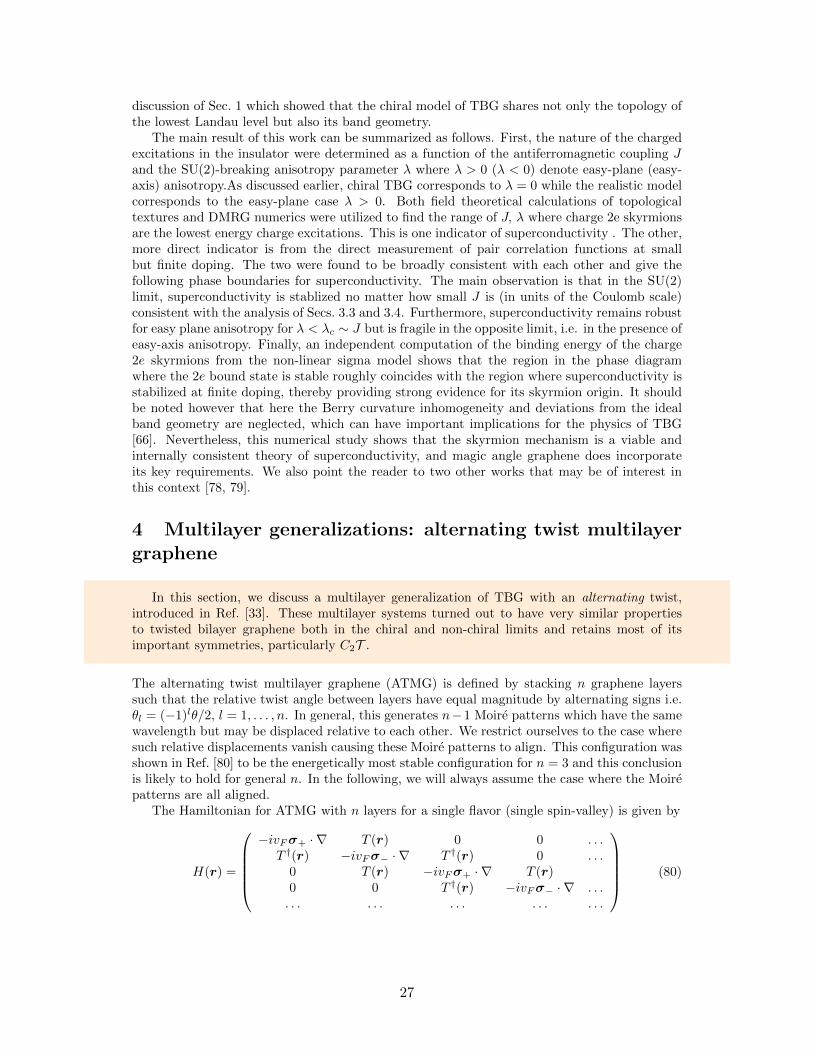
discussion of Sec. 1 which showed that the chiral model of TBG shares not only the topology ofthe lowest Landau level but also its band geometry.

The main result of this work can be summarized as follows. First, the nature of the chargedexcitations in the insulator were determined as a function of the antiferromagnetic coupling Jand the SU(2)-breaking anisotropy parameter λ where λ > 0 (λ < 0) denote easy-plane (easy-axis) anisotropy.As discussed earlier, chiral TBG corresponds to λ = 0 while the realistic modelcorresponds to the easy-plane case λ > 0. Both field theoretical calculations of topologicaltextures and DMRG numerics were utilized to find the range of J, λ where charge 2e skyrmionsare the lowest energy charge excitations. This is one indicator of superconductivity . The other,more direct indicator is from the direct measurement of pair correlation functions at smallbut finite doping. The two were found to be broadly consistent with each other and give thefollowing phase boundaries for superconductivity. The main observation is that in the SU(2)limit, superconductivity is stablized no matter how small J is (in units of the Coulomb scale)consistent with the analysis of Secs. 3.3 and 3.4. Furthermore, superconductivity remains robustfor easy plane anisotropy for λ < λc ∼ J but is fragile in the opposite limit, i.e. in the presence ofeasy-axis anisotropy. Finally, an independent computation of the binding energy of the charge2e skyrmions from the non-linear sigma model shows that the region in the phase diagramwhere the 2e bound state is stable roughly coincides with the region where superconductivity isstabilized at finite doping, thereby providing strong evidence for its skyrmion origin. It shouldbe noted however that here the Berry curvature inhomogeneity and deviations from the idealband geometry are neglected, which can have important implications for the physics of TBG[66]. Nevertheless, this numerical study shows that the skyrmion mechanism is a viable andinternally consistent theory of superconductivity, and magic angle graphene does incorporateits key requirements. We also point the reader to two other works that may be of interest inthis context [78, 79].

4 Multilayer generalizations: alternating twist multilayergraphene

In this section, we discuss a multilayer generalization of TBG with an alternating twist,introduced in Ref. [33]. These multilayer systems turned out to have very similar propertiesto twisted bilayer graphene both in the chiral and non-chiral limits and retains most of itsimportant symmetries, particularly C2T .

The alternating twist multilayer graphene (ATMG) is defined by stacking n graphene layerssuch that the relative twist angle between layers have equal magnitude by alternating signs i.e.θl = (−1)lθ/2, l = 1, . . . , n. In general, this generates n−1 Moire patterns which have the samewavelength but may be displaced relative to each other. We restrict ourselves to the case wheresuch relative displacements vanish causing these Moire patterns to align. This configuration wasshown in Ref. [80] to be the energetically most stable configuration for n = 3 and this conclusionis likely to hold for general n. In the following, we will always assume the case where the Moirepatterns are all aligned.

The Hamiltonian for ATMG with n layers for a single flavor (single spin-valley) is given by

H(r) =

−ivFσ+ · ∇ T (r) 0 0 . . .

T †(r) −ivFσ− · ∇ T †(r) 0 . . .0 T (r) −ivFσ+ · ∇ T (r)0 0 T †(r) −ivFσ− · ∇ . . .. . . . . . . . . . . . . . .

(80)

27

where σ± = e±i4 θσZσe∓

i4 θσz and T (r) is given by

T (r) =

(w0U0(r) w1U1(r)w1U

∗1 (−r) w0U0(r)

), Um(r) =

3∑n=1

e2πi3 m(n−1)e−iqn·r, (81)

qn = 2kD sin

(θ

2

)R 2π(n−1)

3(0,−1) (82)

where Rφ denotes counter clockwise rotation by φ and kD = 4π3√

3aCC.

A remarkable result proved in Ref. [33] is that the Hamiltonian (80) maps to m copiesof TBG with rescaled tunneling matrices T for n = 2m and to m copies of TBG (also withrescaled tunneling matrices T ) in addition to a single Dirac cone for n = 2m + 1. To establishthis mapping, we follow Ref. [33] and perform the transformation H = PTHP with P definedas

P =

bn/2c∑k=1

δ2k,dn/2e+k +

dn/2e∑k=1

δ2k−1,k (83)

This transformation simply relabels the layers such that the Hamiltonian has a block matrixstructure in the even-odd layer index

H = PTHP =

(−ivFσ+ · ∇ T (r)⊗WT †(r)⊗W † −ivFσ− · ∇

), (84)

with W being an dn/2e × bn/2c describing the structure of the tunneling between layers. Sincetunneling only takes place between nearest neighboring layers, W has the simple form Wij =δi,j + δi,j+1. The mapping can be established by writing the singular value decomposition forW = AΛB† which implies that

H ′ =

(A† 00 B†

)H

(A 00 B

)=

(−ivFσ+ · ∇ T (r)⊗ ΛT †(r)⊗ Λ† −ivFσ− · ∇

)(85)

Here, Λ is a diagonal matrix with eigenvalues λk = 2 cos πkn+1 where k = 1, . . . , bn/2c. For even n,

this means that the Hamiltonian H ′ decomposes into a sum of n/2 TBG Hamiltonians with thetunneling T (r) rescaled by λk. For odd n, the matrix Λ is a rectangular (n− 1)/2× (n+ 1)/2matrix. As a result, the Hamiltonian H ′ reduces to (n − 1)/2 TBG Hamiltonians with thetunneling T (r) rescaled by λk in addition to a single Dirac cone that is decoupled from the restof the system. The general unitary matrix which maps H to a decoupled sum of TBGs possiblyin addition to a Dirac cone has the explicit form

Hdec = V †HV, V = P

(A 00 B

)PT (86)

The different TBG systems can be approximately understood as corresponding to differentmomenta along the z direction with the subtlety that there is no true translation in the verticaldirection due to the absence of periodic boundary condition (since the topmost and bottomlayers are not connected by tunneling).

4.1 Trilayer n = 3

The simplest example of ATMG corresponds to the trilayer case with n = 3. The Hamiltonianfor this case is given explicitly by

H(r) =

−ivFσ+ · ∇ T (r) 0T †(r) −ivFσ− · ∇ T †(r)

0 T (r) −ivFσ+ · ∇

(87)

28

The matrix P given explicitly by

P =

1 0 00 0 10 1 0

=⇒ H = PTHP =

−ivFσ+ · ∇ 0 T (r)0 −ivFσ+ · ∇ T (r)

T †(r) T †(r) −ivFσ− · ∇

(88)

The tunneling matrix W and its singular value decomposition W = AΛB† are given by

W =

(11

), =⇒ A =

1√2

(1 −11 1

), Λ =

( √2

0

), B = 1 (89)

Combining these two, we can construct the unitary matrix V which decouples H given explicitlyby

V = P

(A 00 B

)PT =

1√2

0 − 1√2

0 1 01√2

0 1√2

(90)

=⇒ Hdec = V †HV =

−ivFσ+ · ∇√

2T (r) 0√2T †(r) −ivFσ− · ∇ 0

0 0 −ivFσ+ · ∇

(91)

The mapping can be simply understood in terms by noting that the TBG blocks consists ofthe middle layer and the bonding combination of the top and bottom layers whereas the singleDirac cone consists of the anti-bonding combination. The rescaling of the interlayer tunnelingby√

2 means that the magic angles of the trilayer system are larger by a factor of√

2 comparedto TBG magic angles. In particular, the first magic angle is θ ≈ 1.5o.

4.2 Tetralayer n = 4

We can similarly work out the Hamiltonian for the tetralayer case n = 4. The Hamiltonian forthis case is given explicitly by

H(r) =

−ivFσ+ · ∇ T (r) 0 0

T †(r) −ivFσ− · ∇ T †(r) 00 T (r) −ivFσ+ · ∇ T (r)0 0 T †(r) −ivFσ− · ∇

(92)

The matrix P given explicitly by

P =

1 0 0 00 0 1 00 1 0 00 0 0 1

(93)

The tunneling matrix W and its singular value decomposition W = AΛB† are given by

W =

(1 01 1

)=⇒ A =

√3−ϕ

5 −√

2+ϕ5√

2+ϕ5

√3−ϕ

5

, Λ =

(ϕ 00 1/ϕ

), B =

√2+ϕ

5 −√

3−ϕ5√

3−ϕ5

√2+ϕ

5

(94)

29

where ϕ is the golden ratio ϕ = 1+√

52 . The decoupling matrix V is

V =

√3−ϕ

5 0 −√

2+ϕ5 0

0√

2+ϕ5 0 −

√3−ϕ

5√2+ϕ

5 0√

3−ϕ5 0

0√

3−ϕ5 0

√2+ϕ

5

(95)

=⇒ Hdec = V †HV =

−ivFσ+ · ∇ ϕT (r) 0 0ϕT †(r) −ivFσ− · ∇ 0 0

0 0 −ivFσ+ · ∇ 1ϕT (r)

0 0 1ϕT†(r) −ivFσ− · ∇

(96)

Thus, the tetralayer system maps to a pair of TBGs whose interlayer tunneling is scaled by ϕand 1/ϕ. This yields two sequences of magic angles obtained from TBG magic angles either bymultiplying or dividing by the golden ratio ϕ [33]. This mapping can also be understood in termsof bonding and antibonding orbitals as follows. The first TBG (with T rescaled by ϕ) is builtusing the bonding orbitals between the first and third (layer 1) and second and fourth (layer2) whereas the second TBG (with T rescaled by 1/ϕ) is built using the antibonding orbitalsbetween the first and third (as layer 1) and second and fourth (as layer 2).

5 Discussion and Conclusions

In his 1977 Nobel Lecture, Phil Anderson observes:

The art of model-building is the exclusion of real but irrelevant parts of the problem,and entails hazards for the builder and the reader.

In keeping with this spirit, we note that our perspective on magic angle graphene effectivelybegins by approaching the problem from the chiral limit, although several realistic features aresubsequently included. In this limit, the flat bands take the form of zero modes of a Diracoperator, which can be analytically obtained. Further, not just the single particle states buteven the interacting ground state at certain integer fillings can be reliably found in this limit,which are insulators with a generalized flavor order. The topology of the bands ensures the flavororder and the charge physics are inter-related. This has implications for finite doping, and wediscussed a plausible topological mechanism for superconductivity. Other states at fractionalfilling, notably fractional Chern insulators, are also potentially stabilized due to the specialband geometry of the flat bands that resemble that of the lowest Landau level. We believe thisviewpoint broadly captures the observed physics and makes predictions for future experiment.At the same time, let us mention some of the complexities that have been left out. First,although tunneling between opposite Chern bands is retained, which is a significant source ofdispersion, the intra-Chern band dispersion is neglected. Second, the potentially important roleof moire lattice strain, as well as of phonons was not discussed. These and other approximations(such as anisotropies in the sigma model) could alter the energetics of charge carriers, i.e. thecompetition between charge 2e skyrmions and electrons. For small doping, charge could beadded as electrons/holes, and only later intersect the 2e-skyrmion energy. Developing a theoryof such Fermi-Bose models will be an interesting and important task for the future, related tothe quest for a weak coupling version of the same pairing mechanism.

Another important direction is to design experimental probes to identify subtle flavor orders(such as intervally coherence, in particular K-IVC, featuring spatially modulated currents) whichwould be instrumental in both detecting such order in insulators, and tracking their evolutionon doping. One route to identifying the flavor ordered state is by detecting the collective modesassociated with the ground state [66]. These modes can serve as a fingerprint of the flavor orderand also help pin down key parameters like the flavor stiffness, and anisotropies, J and λ.

30

6 Acknowledgements

We would like to thank N. Bultinck, S. Chatterjee, A. Kruchkov, J. Y. Lee, S. Liu, G. Tarnopol-sky and M. Zaletel for collaborations summarized in this work. AV was supported by a SimonsInvestigator award and by the Simons Collaboration on Ultra-Quantum Matter, which is agrant from the Simons Foundation (651440, AV). EK was supported by the German NationalAcademy of Sciences Leopoldina through grant LPDS 2018-02 Leopoldina fellowship. P.J.L. waspartly supported by the Department of Defense (DoD) through the National Defense Scienceand Engineering Graduate Fellowship (NDSEG) Program

A Symmetries of the chiral model

The main feature of the chiral TBG Hamiltonian is the presence of a chiral or sublattice sym-metry which anticommutes with the single-particle Hamiltonian σz, H = 0. In addition,weak-spin orbit coupling in graphene implies that H is invariant under SU(2) spin rotations,i.e. H ∝ s0. The large momentum separation between the graphene valleys leads to valleydecoupling at low energies relevant to TBG physics which implies independent spin and chargeconservation in each valley i.e. H is diagonal in the valley index τz. The two valley are relatedby spinless time-reversal symmetry which is implemented as T = τxK with K denoting complexconjugation, such that HK′(k) = HK(−k)∗. The single particle Hamiltonian is also invariantunder two-fold rotation symmetry which flips sublattice and valley C2 = σxτx. The combi-nation of the two C2T = σxK leaves the valley index invariant and relates the two sublatticewavefunctions at the same momentum k.

A more subtle symmetry of the chiral TBG Hamiltonian is a particle-hole symmetryH(−k)∗ =µyσxH(k)µyσx where µ denote the Pauli matrices in layer space [81, 82]. On the level ofthe single-particle Hamiltonian this is an antiunitary anticommuting symmetry given by P =iµyσxK whereas in second quantized language, this is a unitary particle-hole symmetry actingas

P−1fkP = µyσxf†−k, P−1iP = i (97)

where fk denotes the annihilation operators for microscopic electrons. In addition to the sub-lattice, valley, and spin indices, these electrons also carry a layer index.

Since the chiral symmetry σz is anticommuting and unitary ( anti-unitary particle-hole insecond quantization), T is commuting and anti-unitary (anti-unitary in second quantization),and P is anti-commuting and anti-unitary (unitary particle-hole in second quantization), theirproduct R = iσzPT = τxσyµy is a Z2 unitary commuting symmetry. This extra “hidden”symmetry relates different valley, sublattice and layer indices and leads to enhanced symmetryof the interacting problem as we will see below.

A.1 Symmetries and the Form Factor

Let us now see how that symmetries restrict the structure of the form factor Λq(k). Due to theSU(2) spin rotation symmetry, the spin index does not play any role in the following discussion soit can be dropped. This essentially corresponds to considering a spinless version of the problem.In the following, we will write out the flat band index α in terms of the sublattice-valley indicesσ and τ . We note that sublattice symmetry implies that Λq(k) is diagonal in the sublatticeindex since

〈uA,τ,k|uB,τ,k′〉 = 〈uA,τ,k|σ2z |uB,τ,k′〉 = −〈uA,τ,k|uB,τ,k′〉 = 0 (98)

where we used σz|uA/B,τ,k′〉 = ±|uA/B,τ,k′〉. In addition, valley symmetry implies that Λq(k)is also diagonal in valley. We now note that since R symmetry flips both valley and sublattice,we have

Ruσ,τ,k = eiφσ,τ,ku−σ,−τ,k (99)

for some phase φσ,τ,k. Since we are free to choose the gauge independently in the two valleysτ = ± = K/K ′ and sublattices σ = ± = A/B, we can set φσ,τ,k to 0 by fixing the gauge e.g. in

31

valley K ′ relative to K. This means that we can choose the action of R on the flat bands to beσxτx

7. Similarly, we can deduce the representation of C2T on the flat bands by noting that itflips sublattice but not momentum

C2T uσ,τ,k = eiησ,τ,ku∗−σ,τ,k (100)

The phase factors ησ,τ,k are not completely free since we want to preserve the relation C2T RC2T =−R satisfied by the microscopic operators which implies that η−σ,−τ,k = ησ,τ,k + π. Otherwise,we have the freedom to choose the relative phase between the wavefunctions in sublattices A andB such that ηA,K,k = ηB,K,k = 0 which implies ηA,K′,k = ηB,K′,k = π. This means that C2Tacts as σxτzK in the flat band basis. Note that the action of any of the remaining symmetries,e.g. T or C2, on the flat band will contain extra phase factors that cannot be removed. Inparticular, it can be shown that the band topology enforces a non-trivial phase factors for C2

symmetry [37].Using Eq. 99, we can relate the diagonal entries of the form factor between σ, τ and −σ,−τ

〈uσ,τ,k|uσ,τ,k+q〉 = 〈uσ,τ,k|R2|uσ,τ,k+q〉 = 〈u−σ,−τ,k|u−σ,−τ,k+q〉, (101)

This can be used to relate the form factors in opposite valleys at the same momentum. Inaddition, we can use Eq. 100 to related the form factors within the same valley for the twosublattices leading to

〈uσ,τ,k|uσ,τ,k+q〉 = 〈uσ,τ,k|(C2T )2|uσ,τ,k+q〉 = 〈u−σ,τ,k|u−σ,τ,k+q〉∗ (102)

Thus, the diagonal entries of the form factor are related by complex conjugation upon exchangingsublattice or valley but remain the same under exchanging both. This leads to the followingsimple form of the form factor matrix

Λq(k) = Fq(k)eiΦq(k)σzτz (103)

where Fq(k) and Φq(k) are scalars. Note that the form factor of a given flat band only dependson the combination σzτz which corresponds to the Chern number. This flips under exchangingsublattice (under C2T symmetry), or valley (under T ) but remains invariant under flipping both(under C2 symmetry).

A.2 Symmetries and the Kinetic Term

Different symmetries restrict the form of the single particle term h(k). Our main assumptionis that, although its value may be renormalized by interactions, it has the same symmetries asthe projected chiral BM Hamiltonian (37). First, we can again use spin and valley symmetriesto deduce h(k) is proportional to s0 and diagonal in valley index. For a single valley, h(k) isstricly off-diagonal in sublattice index since:

〈uσ,τ,k|HBM(k)|uσ,τ,k〉 = −〈uσ,τ,k|σzHBM(k)σz|uσ,τ,k〉 = −〈uσ,τ,k|HBM(k)|uσ,τ,k〉 = 0 (104)

This means that the matrix h(k) can only contain the terms σx, σy, σxτz, and σyτz. We can usethe R symmetry to restrict this form further using

〈uσ,τ,k|HBM(k)|uσ′,τ ′,k〉 = 〈uσ,τ,k|RHBM(k)R|uσ′,τ ′,k〉 = 〈u−σ,−τ,k|HBM(k)|u−σ′,−τ ′,k〉 (105)

which implies that h(k) commutes with σxτx excluding the terms σy and σxτz. This leads tothe form

h(k) = hx(k)σx + hy(k)σyτz (106)

7Note that this gauge choise is slightly different from the one used in Ref. [37]

32

A.3 Deviations from the chiral limit

Let us now consider what happens when we deviate from the chiral limit w0 = 0. In this case,chiral symmetry is broken which means that the unitary symmetry R is also broken. As a result,we do not expect the form factors to be diagonal in the sublattice index since the wavefunctionsare no longer completely sublattice polarized. We can still use valley and spin symmetries toshow that the form factor is diagonal in valley and proportional to the identity in spin space.

To restrict the form factor further, we note that the particle-hole symmetry P remains asymmetry to a good approximation provided we assume the angle is small 8. We note thatthe product of P and T anticommutes with the single particle Hamiltonian which means thatthe action of PT = µyτxσx maps positive energy states to negative energy states at the samemomentum k. As a result, it leave the space of flat bands invariant and we can write

PT uσ,τ,k = eiϕσ,τ,ku−σ,−τ,k (107)

To be compatible with the gauge choice in Appendix A.1, we choose the gauge such that PT =iσzR = σyτx which implies that the form factor satisfies σyτxΛq(k)σyτx = Λq(k). This restrictsthe form factor to the terms τ0σ0,y and τzσx,z. In addition, we can use C2T (cf. Eq. 100) to get

〈uσ,τ,k|uσ′,τ,k+q〉 = 〈uσ,τ,k|(C2T )2|uσ′,τ,k+q〉 = 〈u−σ,τ,k|u−σ′,τ,k+q〉∗ (108)

which yields Λq(k) = σxΛq(k)∗σx which implies that the coefficients of τ0σ0, τ0σx and τzσy arereal while the coefficient of τzσz is imaginary leading to the form

Λq(k) = Fq(k)eiΦq(k)σzτz + σxτzFq(k)eiΦq(k)σzτz (109)

Compared to Eq. 103, there is an extra sublattice off-diagonal term which is only non-vanishingaway from the chiral limit.

B Perturbative correction to energy due to single-particledisperison h

To compute the perturbative correction to energy due to single-particle disperison h, we write∆E = J(n+ ·n−−1) and take n+ = −n− = z. We see that the contribution from the tunneling∆E is equal to twice the contribution from tunneling connecting a single fully filled Chern bandto a single fully empty band in the opposite Chern sector. This means we can restrict ourselvesto a pair of tunnel-coupled opposite Chern bands and just multiply the result by 2 9. Fordefiniteness, we take the positive Chern band to be fully filled and the negative Chern band tobe fully empty such that the total number of electrons in the ± band is N+ = N and N− = 0.The single particle “tunneling” term has the form

h =∑k

c†kh(k)ck =∑k

c†+,k[hx(k)− ihy(k)]c−,k + h.c. (110)

where ck = (c+,k, c−,k) is a 2-component vector with annihilation operators in the ± Chern

band. h does not conserve the particle number in each Chern sector separately. Acting with inon a state with (N+, N−) = (N, 0) yields a state with (N+, N−) = (N − 1, 1) with an electronhole pair at some momentum k which can be written as

|Ψk〉 = c†−,kc+,k|Ψ0〉 (111)

8it is only a symmetry if we ignore the angular rotation in the Pauli matrices in Eq. 3 which is equivalent to thereplacemntsuch that σ±θ/2 7→ σ

9the factor of 2 cancels out due to our definition of J with ∆E = −2J such that the absolute value of the resultis precisely J

33

The interacting part of the Hamiltonian conserves momentum and Chern number so it maps thestate |Ψk〉 to a state |Ψk′〉 and it determines the energy spectrum of the particle-hole excitations.As a result, the second order correction to the energy can be written as

∆E = − 1

N

∑k,k′

[hx(k) + ihy(k)][Heh]−1k,k′ [hx(k)− ihy(k)], (112)

with Heh given by [37]

[Heh]k,k′ =1

2A

∑q

Vq〈Ψk|δρqδρ−q|Ψk′〉 =1

A

∑q

VqFq(k)2[δk,k′ − δk′,[k+q]e2iΦq(k)] (113)

where [q] denotes the part of q within the first Moire Brillouin zone.

References

[1] Y. Cao, V. Fatemi, S. Fang, K. Watanabe, T. Taniguchi, E. Kaxiras, and P. Jarillo-Herrero, “Unconventional superconductivity in magic-angle graphene superlattices,” Na-ture, vol. 556, pp. 43–50, Apr 2018.

[2] Y. Cao, V. Fatemi, A. Demir, S. Fang, S. L. Tomarken, J. Y. Luo, J. D. Sanchez-Yamagishi,K. Watanabe, T. Taniguchi, E. Kaxiras, R. C. Ashoori, and P. Jarillo-Herrero, “Correlatedinsulator behaviour at half-filling in magic-angle graphene superlattices,” Nature, vol. 556,pp. 80–84, Apr 2018.

[3] J. M. B. Lopes dos Santos, N. M. R. Peres, and A. H. Castro Neto, “Graphene bilayer witha twist: Electronic structure,” Phys. Rev. Lett., vol. 99, p. 256802, Dec 2007.

[4] G. Li, A. Luican, J. M. B. Lopes dos Santos, A. H. Castro Neto, A. Reina, J. Kong, andE. Y. Andrei, “Observation of van hove singularities in twisted graphene layers,” NaturePhysics, vol. 6, pp. 109–113, Feb 2010.

[5] G. Trambly de Laissardiere, D. Mayou, and L. Magaud, “Localization of dirac electrons inrotated graphene bilayers,” Nano Letters, vol. 10, pp. 804–808, Mar 2010.

[6] E. J. Mele, “Commensuration and interlayer coherence in twisted bilayer graphene,” Phys.Rev. B, vol. 81, p. 161405, Apr 2010.

[7] A. Luican, G. Li, A. Reina, J. Kong, R. R. Nair, K. S. Novoselov, A. K. Geim, and E. Y.Andrei, “Single-layer behavior and its breakdown in twisted graphene layers,” Phys. Rev.Lett., vol. 106, p. 126802, Mar 2011.

[8] R. Bistritzer and A. H. MacDonald, “Moire bands in twisted double-layer graphene,” Pro-ceedings of the National Academy of Sciences, vol. 108, no. 30, pp. 12233–12237, 2011.

[9] J. M. B. Lopes dos Santos, N. M. R. Peres, and A. H. Castro Neto, “Continuum model ofthe twisted graphene bilayer,” Phys. Rev. B, vol. 86, p. 155449, Oct 2012.

[10] D. Wong, Y. Wang, J. Jung, S. Pezzini, A. M. DaSilva, H.-Z. Tsai, H. S. Jung, R. Khajeh,Y. Kim, J. Lee, S. Kahn, S. Tollabimazraehno, H. Rasool, K. Watanabe, T. Taniguchi,A. Zettl, S. Adam, A. H. MacDonald, and M. F. Crommie, “Local spectroscopy of moire-induced electronic structure in gate-tunable twisted bilayer graphene,” Phys. Rev. B,vol. 92, p. 155409, Oct 2015.

[11] K. Kim, A. DaSilva, S. Huang, B. Fallahazad, S. Larentis, T. Taniguchi, K. Watanabe, B. J.LeRoy, A. H. MacDonald, and E. Tutuc, “Tunable moire bands and strong correlationsin small-twist-angle bilayer graphene,” Proceedings of the National Academy of Sciences,vol. 114, no. 13, pp. 3364–3369, 2017.

[12] S. Huang, K. Kim, D. K. Efimkin, T. Lovorn, T. Taniguchi, K. Watanabe, A. H. Mac-Donald, E. Tutuc, and B. J. LeRoy, “Topologically protected helical states in minimallytwisted bilayer graphene,” Phys. Rev. Lett., vol. 121, p. 037702, Jul 2018.

34

[13] P. Rickhaus, J. Wallbank, S. Slizovskiy, R. Pisoni, H. Overweg, Y. Lee, M. Eich, M.-H.Liu, K. Watanabe, T. Taniguchi, T. Ihn, and K. Ensslin, “Transport through a networkof topological channels in twisted bilayer graphene,” Nano Letters, vol. 18, pp. 6725–6730,Nov 2018.

[14] L. Balents, C. R. Dean, D. K. Efetov, and A. F. Young, “Superconductivity and strongcorrelations in moire flat bands,” Nature Physics, vol. 16, pp. 725–733, Jul 2020.

[15] P. W. Anderson, “The resonating valence bond state in la2cuo4 and superconductivity,”Science, vol. 235, no. 4793, pp. 1196–1198, 1987.

[16] H. C. Po, L. Zou, A. Vishwanath, and T. Senthil, “Origin of mott insulating behavior andsuperconductivity in twisted bilayer graphene,” Phys. Rev. X, vol. 8, p. 031089, Sep 2018.

[17] H. C. Po, L. Zou, T. Senthil, and A. Vishwanath, “Faithful tight-binding models and fragiletopology of magic-angle bilayer graphene,” Physical Review B, vol. 99, May 2019.

[18] J. Ahn, S. Park, and B.-J. Yang, “Failure of Nielsen-Ninomiya Theorem and Fragile Topol-ogy in Two-Dimensional Systems with Space-Time Inversion Symmetry: Application toTwisted Bilayer Graphene at Magic Angle,” Physical Review X, vol. 9, p. 021013, Apr2019.

[19] Z. Song, Z. Wang, W. Shi, G. Li, C. Fang, and B. A. Bernevig, “All magic angles in twistedbilayer graphene are topological,” Phys. Rev. Lett., vol. 123, p. 036401, Jul 2019.

[20] J. Kang and O. Vafek, “Symmetry, maximally localized wannier states, and a low-energymodel for twisted bilayer graphene narrow bands,” Phys. Rev. X, vol. 8, p. 031088, Sep2018.

[21] S. Carr, S. Fang, Z. Zhu, and E. Kaxiras, “Minimal model for low-energy electronic statesof twisted bilayer graphene,” arXiv e-prints, p. arXiv:1901.03420, Jan 2019.

[22] G. Tarnopolsky, A. J. Kruchkov, and A. Vishwanath, “Origin of magic angles in twistedbilayer graphene,” Phys. Rev. Lett., vol. 122, p. 106405, Mar 2019.

[23] S. Becker, M. Embree, J. Wittsten, and M. Zworski, “Spectral characterization of magicangles in twisted bilayer graphene,” 2020.

[24] F. K. Popov and A. Milekhin, “Hidden wave function of twisted bilayer graphene: Flatband as a landau level,” 2020.

[25] J. Wang, Y. Zheng, A. J. Millis, and J. Cano, “Chiral approximation to twisted bilayergraphene: Exact intra-valley inversion symmetry, nodal structure and implications forhigher magic angles,” 2020.

[26] G. G. Naumis, L. A. Navarro-Labastida, and E. Aguilar-Mendez, “Reduction of the twistedbilayer graphene chiral hamiltonian into a 2×2 matrix operator and physical origin of flat-bands at magic angles,” 2021.

[27] Y. Ren, Q. Gao, A. MacDonald, and Q. Niu, “Wkb estimate of bilayer graphene’s magictwist angles,” Physical Review Letters, vol. 126, Jan 2021.

[28] E. Khalaf, S. Chatterjee, N. Bultinck, M. P. Zaletel, and A. Vishwanath, “Chargedskyrmions and topological origin of superconductivity in magic-angle graphene,” ScienceAdvances, vol. 7, no. 19, 2021.

[29] S. Chatterjee, N. Bultinck, and M. P. Zaletel, “Symmetry breaking and skyrmionic trans-port in twisted bilayer graphene,” Phys. Rev. B, vol. 101, p. 165141, Apr 2020.

[30] A. Abanov and P. Wiegmann, “Theta-terms in nonlinear sigma-models,” Nuclear PhysicsB, vol. 570, no. 3, pp. 685–698, 2000.

[31] T. Grover and T. Senthil, “Topological spin hall states, charged skyrmions, and supercon-ductivity in two dimensions,” Phys. Rev. Lett., vol. 100, p. 156804, Apr 2008.

[32] D. Li, K. Lee, B. Y. Wang, M. Osada, S. Crossley, H. R. Lee, Y. Cui, Y. Hikita, and H. Y.Hwang, “Superconductivity in an infinite-layer nickelate,” Nature, vol. 572, pp. 624–627,Aug 2019.

35

[33] E. Khalaf, A. J. Kruchkov, G. Tarnopolsky, and A. Vishwanath, “Magic angle hierarchy intwisted graphene multilayers,” Phys. Rev. B, vol. 100, p. 085109, Aug 2019.

[34] R. Bistritzer and A. H. MacDonald, “Moire bands in twisted double-layer graphene,” Pro-ceedings of the National Academy of Sciences, vol. 108, no. 30, pp. 12233–12237, 2011.

[35] N. N. T. Nam and M. Koshino, “Lattice relaxation and energy band modulation in twistedbilayer graphene,” Phys. Rev. B, vol. 96, p. 075311, Aug 2017.

[36] P. J. Ledwith, G. Tarnopolsky, E. Khalaf, and A. Vishwanath, “Fractional chern insulatorstates in twisted bilayer graphene: An analytical approach,” Phys. Rev. Research, vol. 2,p. 023237, May 2020.

[37] N. Bultinck, E. Khalaf, S. Liu, S. Chatterjee, A. Vishwanath, and M. P. Zaletel, “Groundstate and hidden symmetry of magic-angle graphene at even integer filling,” Phys. Rev. X,vol. 10, p. 031034, Aug 2020.

[38] M. M. Fogler, “Stripe and bubble phases in quantum hall systems,” arXiv preprintarXiv:cond-mat/0111001, Nov 2001.

[39] A. L. Sharpe, E. J. Fox, A. W. Barnard, J. Finney, K. Watanabe, T. Taniguchi, M. A.Kastner, and D. Goldhaber-Gordon, “Emergent ferromagnetism near three-quarters fillingin twisted bilayer graphene,” Science, vol. 365, no. 6453, pp. 605–608, 2019.

[40] M. Serlin, C. L. Tschirhart, H. Polshyn, Y. Zhang, J. Zhu, K. Watanabe, T. Taniguchi,L. Balents, and A. F. Young, “Intrinsic quantized anomalous hall effect in a moire het-erostructure,” Science, vol. 367, no. 6480, pp. 900–903, 2020.

[41] Y.-H. Zhang, D. Mao, and T. Senthil, “Twisted bilayer graphene aligned with hexagonalboron nitride: Anomalous hall effect and a lattice model,” Phys. Rev. Research, vol. 1,p. 033126, Nov 2019.

[42] N. Bultinck, S. Chatterjee, and M. P. Zaletel, “Mechanism for anomalous hall ferromag-netism in twisted bilayer graphene,” Phys. Rev. Lett., vol. 124, p. 166601, Apr 2020.

[43] M. Xie and A. H. MacDonald, “Nature of the correlated insulator states in twisted bilayergraphene,” Phys. Rev. Lett., vol. 124, p. 097601, Mar 2020.

[44] F. D. M. Haldane and E. H. Rezayi, “Periodic laughlin-jastrow wave functions for thefractional quantized hall effect,” Phys. Rev. B, vol. 31, pp. 2529–2531, Feb 1985.

[45] F. D. M. Haldane, “Fractional quantization of the hall effect: A hierarchy of incompressiblequantum fluid states,” Phys. Rev. Lett., vol. 51, pp. 605–608, Aug 1983.

[46] S. A. Parameswaran, R. Roy, and S. L. Sondhi, “Fractional chern insulators and the W∞algebra,” Phys. Rev. B, vol. 85, p. 241308, Jun 2012.

[47] R. Roy, “Band geometry of fractional topological insulators,” Phys. Rev. B, vol. 90,p. 165139, Oct 2014.

[48] S. A. Parameswaran, R. Roy, and S. L. Sondhi, “Fractional quantum hall physics in topolog-ical flat bands,” Comptes Rendus Physique, vol. 14, no. 9, pp. 816 – 839, 2013. Topologicalinsulators / Isolants topologiques.

[49] M. Claassen, C. H. Lee, R. Thomale, X.-L. Qi, and T. P. Devereaux, “Position-momentumduality and fractional quantum hall effect in chern insulators,” Phys. Rev. Lett., vol. 114,p. 236802, Jun 2015.

[50] C. Repellin, Z. Dong, Y.-H. Zhang, and T. Senthil, “Ferromagnetism in narrow bands ofmoire superlattices,” Phys. Rev. Lett., vol. 124, p. 187601, May 2020.

[51] A. Abouelkomsan, Z. Liu, and E. J. Bergholtz, “Particle-hole duality, emergent fermiliquids, and fractional chern insulators in moire flatbands,” Phys. Rev. Lett., vol. 124,p. 106803, Mar 2020.

[52] P. Wilhelm, T. C. Lang, and A. M. Lauchli, “Interplay of fractional chern insulator andcharge density wave phases in twisted bilayer graphene,” Phys. Rev. B, vol. 103, p. 125406,Mar 2021.

36

[53] S. M. Girvin, “The quantum hall effect: novel excitations and broken symmetries,” in As-pects topologiques de la physique en basse dimension. Topological aspects of low dimensionalsystems, pp. 53–175, Springer, 1999.

[54] S. L. Sondhi, A. Karlhede, S. A. Kivelson, and E. H. Rezayi, “Skyrmions and the crossoverfrom the integer to fractional quantum hall effect at small zeeman energies,” Phys. Rev. B,vol. 47, pp. 16419–16426, Jun 1993.

[55] S. Liu, E. Khalaf, J. Y. Lee, and A. Vishwanath, “Nematic topological semimetal andinsulator in magic-angle bilayer graphene at charge neutrality,” Phys. Rev. Research, vol. 3,p. 013033, Jan 2021.

[56] U. Zondiner, A. Rozen, D. Rodan-Legrain, Y. Cao, R. Queiroz, T. Taniguchi, K. Watanabe,Y. Oreg, F. von Oppen, A. Stern, E. Berg, P. Jarillo-Herrero, and S. Ilani, “Cascade of phasetransitions and dirac revivals in magic-angle graphene,” Nature, vol. 582, pp. 203–208, Jun2020.

[57] D. Wong, K. P. Nuckolls, M. Oh, B. Lian, Y. Xie, S. Jeon, K. Watanabe, T. Taniguchi,B. A. Bernevig, and A. Yazdani, “Cascade of electronic transitions in magic-angle twistedbilayer graphene,” Nature, vol. 582, pp. 198–202, Jun 2020.

[58] T. Cea and F. Guinea, “Band structure and insulating states driven by coulomb interactionin twisted bilayer graphene,” Phys. Rev. B, vol. 102, p. 045107, Jul 2020.

[59] T. Soejima, D. E. Parker, N. Bultinck, J. Hauschild, and M. P. Zaletel, “Efficient simulationof moire materials using the density matrix renormalization group,” Phys. Rev. B, vol. 102,p. 205111, Nov 2020.

[60] D. E. Parker, T. Soejima, J. Hauschild, M. P. Zaletel, and N. Bultinck, “Strain-inducedquantum phase transitions in magic angle graphene,” arXiv preprint arXiv:2012.09885,2020.

[61] J. Kang and O. Vafek, “Non-abelian dirac node braiding and near-degeneracy of correlatedphases at odd integer filling in magic-angle twisted bilayer graphene,” Phys. Rev. B, vol. 102,p. 035161, Jul 2020.

[62] F. Xie, A. Cowsik, Z. Son, B. Lian, B. A. Bernevig, and N. Regnault, “Tbg vi: An ex-act diagonalization study of twisted bilayer graphene at non-zero integer fillings,” arXivpreprint arXiv:2010.00588, 2020.

[63] P. Potasz, M. Xie, and A. H. MacDonald, “Exact diagonalization for magic-angle twistedbilayer graphene,” arXiv preprint arXiv:2102.02256, 2021.

[64] B. A. Bernevig, Z. Song, N. Regnault, and B. Lian, “Tbg iii: Interacting hamiltonian andexact symmetries of twisted bilayer graphene,” arXiv preprint arXiv:2009.12376, 2020.

[65] B. Lian, Z.-D. Song, N. Regnault, D. K. Efetov, A. Yazdani, and B. A. Bernevig, “Tbgiv: Exact insulator ground states and phase diagram of twisted bilayer graphene,” arXivpreprint arXiv:2009.13530, 2020.

[66] E. Khalaf, N. Bultinck, A. Vishwanath, and M. P. Zaletel, “Soft modes in magic angletwisted bilayer graphene,” arXiv preprint arXiv:2009.14827, 2020.

[67] Y. Choi, H. Kim, Y. Peng, A. Thomson, C. Lewandowski, R. Polski, Y. Zhang, H. S. Arora,K. Watanabe, T. Taniguchi, et al., “Tracing out correlated chern insulators in magic angletwisted bilayer graphene,” arXiv preprint arXiv:2008.11746, 2020.

[68] S. Wu, Z. Zhang, K. Watanabe, T. Taniguchi, and E. Y. Andrei, “Chern insulators, van hovesingularities and topological flat bands in magic-angle twisted bilayer graphene,” NatureMaterials, vol. 20, pp. 488–494, Apr 2021.

[69] K. P. Nuckolls, M. Oh, D. Wong, B. Lian, K. Watanabe, T. Taniguchi, B. A. Bernevig, andA. Yazdani, “Strongly correlated chern insulators in magic-angle twisted bilayer graphene,”Nature, vol. 588, pp. 610–615, Dec 2020.

37

[70] Y. Saito, J. Ge, L. Rademaker, K. Watanabe, T. Taniguchi, D. A. Abanin, and A. F. Young,“Hofstadter subband ferromagnetism and symmetry-broken chern insulators in twisted bi-layer graphene,” Nature Physics, vol. 17, pp. 478–481, Apr 2021.

[71] S. Chatterjee, M. Ippoliti, and M. P. Zaletel, “Skyrmion superconductivity: DMRG evi-dence for a topological route to superconductivity,” arXiv preprint arXiv:2010.01144, 2020.

[72] K. Moon, H. Mori, K. Yang, S. M. Girvin, A. H. MacDonald, L. Zheng, D. Yoshioka,and S.-C. Zhang, “Spontaneous interlayer coherence in double-layer quantum hall systems:Charged vortices and kosterlitz-thouless phase transitions,” Phys. Rev. B, vol. 51, pp. 5138–5170, Feb 1995.

[73] A. M. Polyakov and A. A. Belavin, “Metastable States of Two-Dimensional Isotropic Ferro-magnets,” JETP Lett., vol. 22, pp. 245–248, 1975. [Pisma Zh. Eksp. Teor. Fiz.22,503(1975)].

[74] D. R. Nelson and J. M. Kosterlitz, “Universal jump in the superfluid density of two-dimensional superfluids,” Phys. Rev. Lett., vol. 39, pp. 1201–1205, Nov 1977.

[75] A. d’Adda, M. Luscher, and P. Di Vecchia, “A 1n expandable series of non-linear σ modelswith instantons,” Nuclear Physics B, vol. 146, no. 1, pp. 63–76, 1978.

[76] E. Witten, “Instatons, the quark model, and the 1/n expansion,” Nuclear Physics B,vol. 149, no. 2, pp. 285–320, 1979.

[77] A. Polyakov, Gauge Fields and Strings. Contemporary concepts in physics, Taylor &Francis, 1987.

[78] M. Christos, S. Sachdev, and M. S. Scheurer, “Superconductivity, correlated insulators,and wess–zumino–witten terms in twisted bilayer graphene,” Proceedings of the NationalAcademy of Sciences, vol. 117, no. 47, pp. 29543–29554, 2020.

[79] Y. Liu, Z. Wang, T. Sato, M. Hohenadler, C. Wang, W. Guo, and F. F. Assaad, “Supercon-ductivity from the condensation of topological defects in a quantum spin-hall insulator,”Nature Communications, vol. 10, Jun 2019.

[80] S. Carr, C. Li, Z. Zhu, E. Kaxiras, S. Sachdev, and A. Kruchkov, “Ultraheavy and ultrarela-tivistic dirac quasiparticles in sandwiched graphenes,” Nano Letters, vol. 20, pp. 3030–3038,May 2020.

[81] Z. Song, Z. Wang, W. Shi, G. Li, C. Fang, and B. A. Bernevig, “All magic angles in twistedbilayer graphene are topological,” Phys. Rev. Lett., vol. 123, p. 036401, Jul 2019.

[82] K. Hejazi, C. Liu, H. Shapourian, X. Chen, and L. Balents, “Multiple topological transitionsin twisted bilayer graphene near the first magic angle,” Phys. Rev. B, vol. 99, p. 035111,Jan 2019.

38