structural - mdh 4 2 the axe system and the plex language 5 2.1 ... 30 3.3.4 execution time limits...
TRANSCRIPT

A Structural Operational Semantics for
PLEX
Johan Erikson
November 7, 2003

i
Abstract
Programming Language for EXchanges, PLEX, is a single-purpose and
event-based real-time language developed by Ericsson and used in the central
parts of the AXE switching system. The language has a signal paradigm as
its top execution level, and it is event-based in the sense that only events,
encoded as signals, can trigger code execution. This report presents a struc-
tural operational semantics for fundamental parts of the language, i.e., over
jumps and signal sending statements.
The language and its execution model are tightly connected and it is
not possible to separate one from the other. With the semantics presented
in this report, a �rst step towards the semantic de�nition of the execution
model has been taken. The semantics of the execution model is considered
to be a cornerstone in the work of adapting the language to a multi-processor
environment.
Earlier attempts to map the language to description languages, like SDL,
have not been as successful as expected, which is probably due to the fact that
the semantics of the language and its execution model have not been paid
enough attention. With this report, a formal basis for further investigations
in that direction is provided.

ii
Acknowledgments
This report was written mainly between spring and autumn 2002 at
Mälardalen University, Västerås, Sweden. The work is published within
the research co-operation between Ericsson AB and Mälardalen Real-Time
Research Center.
First of all, the author would like to thank Björn Lisper at Mälardalen
University, and Janet Wennersten at Ericsson AB, for supervising this
work.
Secondly, a number of people at Mälardalen University, have helped me
in di�erent ways: I have had many interesting discussions with Peter Funk
and Bo Lindell . Lars Bruce and Jan Gustafsson have both proof read
parts of the material. Markus Bohlin and Jan Carlson have helped me
out when my LATEX and Emacs skills were insu�cient.
Then comes a number of people at Ericsson AB: Per-Åke Ek , Anton
Massoud , Ingvar Nilsson and Lars-Erik Wiman have all helped me
with material and/or discussions.
I would also like to thank Per Burman , Anders R. Larsson and
Anders Skelander at Ericsson AB, as well as Peter Funk (again) at
Mälardalen University, who all have been eager to keep the research co-
operation between Ericsson AB and Mälardalen University �up and running�.
Finally, this work has been founded by Ericsson AB , Mälardalen
Real-Time Research Center and the KK-foundation . Thank you.

Contents
List of Figures vi
List of Tables ix
1 Introduction 1
1.1 Background and Problem De�nition . . . . . . . . . . . . . . 1
1.2 Limitations . . . . . . . . . . . . . . . . . . . . . . . . . . . . 2
1.3 Aim . . . . . . . . . . . . . . . . . . . . . . . . . . . . . . . . 2
1.4 Organization . . . . . . . . . . . . . . . . . . . . . . . . . . . 2
I The Execution Model of APZ/PLEX 4
2 The AXE System and the PLEX Language 5
2.1 The AXE System . . . . . . . . . . . . . . . . . . . . . . . . . 5
2.1.1 Central- and Regional Processors . . . . . . . . . . . . 5
2.1.2 Input and Output statements . . . . . . . . . . . . . . 8
2.1.3 Load, Reload and Dump . . . . . . . . . . . . . . . . . 9
2.2 Programming Language for EXchanges . . . . . . . . . . . . . 10
2.2.1 The structure of a PLEX program . . . . . . . . . . . 11
2.2.2 Records, Files and Pointers . . . . . . . . . . . . . . . 13
2.2.3 Variables . . . . . . . . . . . . . . . . . . . . . . . . . 14
2.2.4 Data Encapsulation . . . . . . . . . . . . . . . . . . . 17
3 The Execution Model 19
3.1 Introduction . . . . . . . . . . . . . . . . . . . . . . . . . . . . 19
3.1.1 PLEX structure and OS requirements . . . . . . . . . 19
3.1.2 Software Units . . . . . . . . . . . . . . . . . . . . . . 19
3.1.3 Function Blocks . . . . . . . . . . . . . . . . . . . . . . 21
iii

iv
3.1.4 Application System . . . . . . . . . . . . . . . . . . . . 21
3.2 Program Interwork - Signals . . . . . . . . . . . . . . . . . . . 21
3.2.1 Direct and bu�ered signals . . . . . . . . . . . . . . . 24
3.2.2 Unique and multiple signals . . . . . . . . . . . . . . . 24
3.2.3 Single and combined signals . . . . . . . . . . . . . . . 25
3.2.4 Local and Non-local signals . . . . . . . . . . . . . . . 26
3.2.5 Signals and Priorities . . . . . . . . . . . . . . . . . . . 27
3.2.6 Signals and Data . . . . . . . . . . . . . . . . . . . . . 27
3.3 Jobs, Signal Bu�ers and Job Handling . . . . . . . . . . . . . 28
3.3.1 What is a Job? . . . . . . . . . . . . . . . . . . . . . . 28
3.3.2 Signal Bu�ers . . . . . . . . . . . . . . . . . . . . . . . 28
3.3.3 Job Handling . . . . . . . . . . . . . . . . . . . . . . . 30
3.3.4 Execution Time Limits . . . . . . . . . . . . . . . . . . 34
3.4 Linking Encapsulation . . . . . . . . . . . . . . . . . . . . . . 34
3.4.1 Addressing a Program Sequence . . . . . . . . . . . . . 35
3.5 Software Recovery . . . . . . . . . . . . . . . . . . . . . . . . 38
3.5.1 Forlopp . . . . . . . . . . . . . . . . . . . . . . . . . . 40
3.5.2 System Restart . . . . . . . . . . . . . . . . . . . . . . 40
3.5.3 Forlopp Release or a System Restart? . . . . . . . . . 42
3.5.4 Variables and Software Recovery . . . . . . . . . . . . 44
II Semantics 45
4 Related Work 46
5 Programming Language Semantics 48
5.1 The meaning of a program . . . . . . . . . . . . . . . . . . . . 48
5.2 Semantic approaches . . . . . . . . . . . . . . . . . . . . . . . 49
5.3 Notation . . . . . . . . . . . . . . . . . . . . . . . . . . . . . . 50
5.4 Operational Semantics . . . . . . . . . . . . . . . . . . . . . . 51
5.4.1 Natural Semantics . . . . . . . . . . . . . . . . . . . . 51
5.4.2 Structural Operational Semantics . . . . . . . . . . . . 52
5.5 Denotational Semantics . . . . . . . . . . . . . . . . . . . . . 53
5.6 Axiomatic Semantics . . . . . . . . . . . . . . . . . . . . . . . 53

v
6 Semantic Approach 55
6.1 Selected Approach and Motivation . . . . . . . . . . . . . . . 55
6.2 The State of the System . . . . . . . . . . . . . . . . . . . . . 56
6.3 Lexical Units and Syntactical Categories . . . . . . . . . . . . 61
6.4 Statements for Variable Assignments . . . . . . . . . . . . . . 65
6.5 Jump Statements . . . . . . . . . . . . . . . . . . . . . . . . . 65
6.6 Conditional Statements . . . . . . . . . . . . . . . . . . . . . 66
6.7 Selections . . . . . . . . . . . . . . . . . . . . . . . . . . . . . 67
6.8 Iterations . . . . . . . . . . . . . . . . . . . . . . . . . . . . . 67
6.9 Signal Sending/Receiving Statements . . . . . . . . . . . . . . 68
6.9.1 Statements for Single Signals . . . . . . . . . . . . . . 69
6.9.2 Statements for Combined Signals . . . . . . . . . . . . 70
6.9.3 Statements for Local Signals . . . . . . . . . . . . . . . 70
6.10 Exit . . . . . . . . . . . . . . . . . . . . . . . . . . . . . . . . 71
6.11 Semantic Functions . . . . . . . . . . . . . . . . . . . . . . . . 71
6.12 The Semantics for Assignment Statements . . . . . . . . . . . 76
6.13 The semantics for Jump statements . . . . . . . . . . . . . . . 77
6.14 The semantics for Conditional statements . . . . . . . . . . . 77
6.15 The semantics for Selection statements . . . . . . . . . . . . . 78
6.16 The semantics for Iteration statements . . . . . . . . . . . . . 78
6.17 The Semantics for Signal Statements . . . . . . . . . . . . . . 81
6.17.1 Single Signals . . . . . . . . . . . . . . . . . . . . . . . 84
6.17.2 Combined Signals . . . . . . . . . . . . . . . . . . . . . 87
6.17.3 The Semantics for Local Signals . . . . . . . . . . . . . 90
6.18 The Semantics for the EXIT-statement . . . . . . . . . . . . . 91
6.19 The Semantic Function SPLEX . . . . . . . . . . . . . . . . . 93
7 Summary 95
Index 97
A The Semantics for PLEX 98
B The Signal Description 106
List of Figures
1.1 This report and its context. . . . . . . . . . . . . . . . . . . . 3
2.1 The hierarchical structure of the AXE system . . . . . . . . . 6
2.2 AM shared between applications . . . . . . . . . . . . . . . . . 6
2.3 Stores in the central processor (CP). (The interaction between
the di�erent stores are covered in Section 3.4.) . . . . . . . . 8
2.4 The I/O system and its communication with the environment. 9
2.5 The di�erent languages used in di�erent parts of the AXE
system . . . . . . . . . . . . . . . . . . . . . . . . . . . . . . . 12
2.6 Structure of the SPI, i.e., a PLEX program �le. . . . . . . . . 14
2.7 An example �le with n records and a pointer with the current
value 2. . . . . . . . . . . . . . . . . . . . . . . . . . . . . . . 15
2.8 Variables and properties (from a storage point of view). . . . . 16
2.9 Permitted combinations of variable properties and variable types. 18
2.10 The structure of a software unit (block). The possibility of
several sub-programs accessing the same data within the block
is shown. All sub-programs (signal entries) can access all DS
variables inside the same block (except for individuals that are
DS variables inside a record). This conveys a DS variable can
be used as a communication channel between all sub-programs
inside the same software unit. . . . . . . . . . . . . . . . . . . 18
3.1 APT Application system. . . . . . . . . . . . . . . . . . . . . . 20
3.2 The di�erent types of software signals. . . . . . . . . . . . . . 22
3.3 A PLEX program �le divided in subprograms. Note that the
assignment CUSELESS = 0; will never be executed since it is
placed between an exit and an enter statement. (See also Fig.
2.6 where a complete program �le is described.) . . . . . . . . 23
vi

vii
3.4 Direct and bu�ered signals. . . . . . . . . . . . . . . . . . . . 24
3.5 Unique and multiple signals. . . . . . . . . . . . . . . . . . . . 25
3.6 Single and combined signals. . . . . . . . . . . . . . . . . . . . 26
3.7 Possible properties for CP-CP signals. X indicates a legal/possible
combination, shaded with Grey indicates an illegal alternative.
NOTE: A combined backward signal can not be multiple
since this signal is an answer (i.e., an acknowledgment) to a
�caller� and must therefore return to the �caller� and nobody
else. . . . . . . . . . . . . . . . . . . . . . . . . . . . . . . . . 26
3.8 Forward and Backward signals. . . . . . . . . . . . . . . . . . 27
3.9 Sending of a delayed (and multiple) signal. The signal is sent
from Unit A and received in Unit C but, as could be seen in
the �gure, it is possible to receive the signal in Unit B as well
if Unit B is speci�ed as the receiver by the PLEX designer. . 30
3.10 Job bu�ers and runtime priorities in the AXE system. . . . . 31
3.11 The execution model - Four jobs are executed. The process
of transferring a bu�ered signal from the sending block to the
receiving, via a job bu�er, is shown in Fig. 3.12. NOTE the
�parallel� architecture that could become real parallel execution. 32
3.12 Linking and execution for a bu�ered signal in APZ. See also
Fig. 3.11. NOTE: The procedure is the same for direct sig-
nals except that they not are inserted in a Job Bu�er. . . . . 33
3.13 PS, showing SDT, SST and Program Code of one function unit. 35
3.14 RS, showing the Reference Table. . . . . . . . . . . . . . . . . 36
3.15 The information �ow in determining the signal entry when
sending a signal. . . . . . . . . . . . . . . . . . . . . . . . . . 36
3.16 The consecutive order of handling a signal sending. . . . . . . 37
3.17 Show how addressing to DS is performed in RS. BSA points
to the starting point of BAT . . . . . . . . . . . . . . . . . . . 39
3.18 Di�erent types of system restart. . . . . . . . . . . . . . . . . 42
3.19 The intensity counter. . . . . . . . . . . . . . . . . . . . . . . 43
3.20 Di�erent levels of recovery after a detected software error. . . 43
3.21 Data security of di�erent start/restart types. . . . . . . . . . . 44
5.1 The compound statement expressed in natural semantics. . . . 52
5.2 The compound statement expressed in structural operational
semantics. . . . . . . . . . . . . . . . . . . . . . . . . . . . . . 53

viii
5.3 The compound statement expressed in denotational semantics. 54
5.4 The compound statement expressed in a axiomatic semantics
style. . . . . . . . . . . . . . . . . . . . . . . . . . . . . . . . . 54
6.1 The di�erent stores in the central processor (CP). . . . . . . . 57
6.2 A simpli�ed �gure of the job bu�ers in the PLEX/AXE envi-
ronment. (See also Fig. 3.10) . . . . . . . . . . . . . . . . . . 58
6.3 The FIFO-semantics of the job bu�ers. . . . . . . . . . . . . . 58
6.4 Organization of the job bu�ers. NOTE: The pointer regis-
ters, W8-W9, are treated as one register (and referred to as
POINTER B0). This is due to the fact that the register in
W9 is only used when a pointer is too large to �t only in W8.
In this case, the pointer will be split up and placed in W8 with
its �rst half, and in W9 with its second half. . . . . . . . . . . 59
6.5 PLEX iteration statements - a comparison. . . . . . . . . . . 68
6.6 The process of �nding the receiver of a bu�ered signal. (Re-
peated from Section 3.3.3, Fig. 3.12.) NOTE: The process is
similar for direct signals, except that they are not inserted in
a Job Bu�er. (See also Figure 6.4 for a detailed description
on the organization of the job bu�ers.) . . . . . . . . . . . . . 83

List of Tables
6.1 Priorities and meaning of the PLEX operators. Priorities are
numbered from the highest (1) to the lowest (8). . . . . . . . . 64
6.2 A summary of the semantic functions de�ned and used in
Chapter 6 (and in Appendix A). . . . . . . . . . . . . . . . . . 72
6.3 The semantics of �arithmetic� expressions. . . . . . . . . . . . 74
6.4 The semantics of �boolean� expressions. (See also, Table 6.1
where the di�erent operators, as well as their meaning, are de-
scribed.) an represents a �eld-expression whereas tn represents
a string. . . . . . . . . . . . . . . . . . . . . . . . . . . . . . . 75
6.5 The function APZ which fetches the �rst �ready-job� with
highest priority. . . . . . . . . . . . . . . . . . . . . . . . . . . 92
ix

Chapter 1
Introduction
1.1 Background and Problem De�nition
The programming language PLEX (Programming Language for EXchanges)
is a single-purpose and event-based real-time language developed by Erics-
son. The language is designed exclusively for telephony systems and used in
central parts of the AXE switching system (from Ericsson). The language
has a signal paradigm as its top execution level, and it is event-based in the
sense that only events, encoded as signals, can trigger code execution.
The language has been continuously evolving since the 1970's when it
was originally designed. But in parallel with this, attempts have been made
to replace it with more �modern� languages like C++ for instance, or speci-
�cation languages like standard SDL. However, most of these attempts have
failed and considerable money has been spent. It is probable that the failure
of replacing PLEX is due to properties of the language and its execution
model, i.e. the semantics of the language has not been paid enough atten-
tion. For example, to use SDL successfully, the unique semantics of PLEX
were considered in creating an extension to SDL, called SDL-10 which could
then be code generated to PLEX.
A second �problem� is the fact that since the semantics of the language
has not been speci�ed before, it is possible to use �ad hoc� solutions in
new implementations of the language, i.e., when a new hardware platform is
introduced.
This report should also be seen in a further perspective, where the aim
is to extend and modify the language with a possibility to run in a multi-
processor environment, see Fig. 1.1. This could already be done today due
1
CHAPTER 1. INTRODUCTION 2
to the modular structure of the language, but as shown by Lindell [Lin03],
there are problems that need to be solved.
1.2 Limitations
This report will focus on the basic concepts of signals since this is consid-
ered to be the most important aspects of the language, and the parts that
most signi�cantly di�erentiate PLEX from other languages. It will give an
operational semantics for the individual PLEX statements, as well as for se-
quences of statements. However, the semantics for sequences of statements is
restricted to well-formed constructs (which will be de�ned in Section 6.19).
1.3 Aim
The aim of this report is to give a semantic de�nition of the most important
parts of PLEX, mentioned in Section 1.2. With this in hand, a formal basis
for further investigations and comparisons with other languages is provided
since the meaning of a (PLEX)program has been given a semantic de�nition.
The semantics will also reveal ambiguities and prevent �ad hoc� solutions
when the language is moved to a new hardware platform.
A second aim is to form the basis for further investigations and develop-
ment of a possible semantic framework for the execution model of PLEX. As
shown in Fig. 1.1, this is one of the steps in modifying PLEX for parallel
execution.
1.4 Organization
This report is structured in two main parts:
� Part I includes the Technical Report �The Execution Model of
APZ/PLEX - An Informal Description� by J. Erikson and B Lindell
[EL02]. This part serves as an introduction to the execution model
of PLEX for the reader not familiar with the language and its envi-
ronment1. This part could be skipped, without any loss, by the reader
familiar with PLEX.
1Also, a general survey of PLEX as well as of the AXE switching system can be found
in [AGG99]

CHAPTER 1. INTRODUCTION 3
� Part II is the main part of this report. This part deals with the
semantics for PLEX. Chapter 5 serves as an introduction to semantic
notation and describes the most common frameworks. Chapter 6 could
be seen as the main chapter of this report, since the semantics for
PLEX is de�ned here. The semantics is developed throughout the
chapter, when we look at the di�erent statements in the language.
Appendix A then summarizes the semantics that are de�ned in Chapter
6.
Formal semantics for theexecutionmodel of
PLEX/APZ
"A StructuralOperational
Semantics for PLEX"(Erikson)
"The Execution Model ofAPZ/PLEX - An Informal
Description"(Erikson & Lindell)
"Analysis of reentrancyand problems of data
interference in the parallelexecution of a multiprocessor AXE-APZ
system"(Lindell)
PLEXExtensions and
Modifications for parallelexecution
Figure 1.1: This report and its context.

Part I
The Execution Model of
APZ/PLEX
4

Chapter 2
The AXE System and the
PLEX Language
2.1 The AXE System
The AXE telephone exchange system from Ericsson, developed in its ear-
liest version in the beginning of the 1970s, is structured in a modular and
hierarchical way. It consists of the two main parts:
APT: The telephony or switching part
APZ: The control part including central and regional processors
which both consist of hardware and software. The two main parts are di-
vided into subsystems or Application Modules (AM). An AM is a group of
blocks with a collection of shared software resources and it only exist in the
APT side, See Fig. 2.2 for an example of how AMs are used. A subsystem is
divided in function blocks. Function blocks consist of function units which
is either a central software unit or a hardware unit, a regional software unit
and a central software unit. The structure of the system is shown in Fig 2.1.
(Note that this is not a complete description of the system.) The parts that
will be of interest in this report is marked with bold text.
2.1.1 Central- and Regional Processors
The hardware aspects that is of interest in this report is the distinction be-
tween Central- and Regional Processors. This is because di�erent forms of
5

CHAPTER 2. THE AXE SYSTEM AND THE PLEX LANGUAGE 6
System Level 1
System Level 2
Subsystem /Application
Module
Function Block
Function Unit
CPS NMS
LIC LIR LIUCJU
AXE
APZ APT
MAS FMS SSS GSS
CJ KR LI
APT - Telephony/Switching part APZ - Control part including central and regional processors
as well as operating system CPS - Central Processor Subsystem MAS - Maintenance Subsystem
AMAM . . .
Figure 2.1: The hierarchical structure of the AXE system
AM AM AM AMAM
Application 1 Application 2
Figure 2.2: AM shared between applications

CHAPTER 2. THE AXE SYSTEM AND THE PLEX LANGUAGE 7
interwork is performed between di�erent kinds of processors. The distinc-
tions are brie�y discussed in this subsection and explained in more detail in
Section 3.2.
Regional Processor (RP): There are several regional processors in an
AXE system. The main task of a regional processor is to relieve the
central processor by handling small routine jobs like scanning and �l-
tering.
Central Processor (CP): This is the central control unit of the system.
All complex and non-trivial decisions are taken in the central proces-
sor. This is the place for all forms of non-routine work. The work
of the processor can be separated into two speci�cally distinct parts,
namely instruction execution and job administration. Instruction exe-
cution means handling of uninterrupted sequences of operations where
the work consists of address table look-up and calculations, plausibility
checks, storage accesses and data manipulations. The job administra-
tion mainly consists of signal handling, signal conversion and signal
bu�er handling. The execution of instructions is a single-stream work
by nature, whereas the job administration to a great extent is a ques-
tion of prioritized job queues (Section 3.3) and transfer of signal data.
The CP is always duplicated. The two sides work in parallel, perform-
ing exactly the same operations. During normal operation, one CP is
executive and the other is stand-by. A continuous check is made to
ensure that both processors reach the same result - If they don't, some
form of recovery action is performed (Section 3.5). The CP duplica-
tion also enables function changes (installation of new software ver-
sions) while the exchange is in an operational mode by �rst installing
new software on the stand-by side and then change the executive and
stand-by order between the processors. As a last step, the new software
is installed on the former executive (now stand-by) side.
The CPs store all central software and data. The CP memory consists
of the register memory and the di�erent stores. Programs are stored in
the program store (PS) and data is stored in the data store (DS). The
reference store contains information about where to �nd the di�erent
programs and data, Fig. 2.3.

CHAPTER 2. THE AXE SYSTEM AND THE PLEX LANGUAGE 8
Program Store
PS
Reference Store
RS
Data Store
DS
Figure 2.3: Stores in the central processor (CP). (The interaction between
the di�erent stores are covered in Section 3.4.)
2.1.2 Input and Output statements
An AXE exchange needs to communicate with its environment and its op-
eration and maintenance (O&M) sta�. Some typical situations could be the
following:
- An exchange technician changes subscriber categories, replaces devices or
connects new subscribers.
- The exchange informs the O&M sta� of important events, e.g., if an RP is
blocked due to a fault. In other words, the I/O statements are an important
part of the recovery mechanism. (See Section 3.5.)
- Input/output includes certain routine tasks to, e.g. dumping data on a
hard disk.
There is a large number of I/O devices used; alarm and hard copy print-
ers, display units, work stations and PC's, magnetic tape drivers, hard and
�exible disks.
Before communicating with an I/O device, the PLEX program has to
seize the device. Likewise, the device has to be released when the com-
munication ends. This guarantees exclusive access to the device. All I/O
devices are connected to a support processor (SP), and function blocks that
receive or send information via the I/O system are called user blocks. Fig.
2.4 shows the interaction between the I/O system and a user block. When
seizing an I/O device, the I/O system assigns a free line bu�er and a free
analysis bu�er (see Fig. 2.4) to this device. These bu�ers temporarily store
the I/O text. The analysis bu�er handles input from the I/O device, and
the line bu�er handles output.
The basic (PLEX) statements for transferring information between the
bu�ers and the I/O device, and between the bu�ers and the user blocks are:
- FETCH: transfer information from the analysis bu�er to the user block.

CHAPTER 2. THE AXE SYSTEM AND THE PLEX LANGUAGE 9
SP
Line Buffer72 Characters
Analysis Buffer144 Characters
I/O System
UserBlock
2 Insert
3 Write
4 Read
1
1 Fetch23
4
Program Store
I/O device
Figure 2.4: The I/O system and its communication with the environment.
- INSERT: transfer information from the user block to the line bu�er.
- WRITE: orders the I/O system to print out the text in the line bu�er to an
I/O device.
- READ: transfer information from the I/O device to the analysis bu�er.
Again, see Fig. 2.4.
Typically, I/O communication starts with the operator entering a com-
mand on an I/O device. The command is received by the I/O system and
delivered to the software unit where it has been de�ned by the programmer.
A command is received in a program (i.e., a software unit) in the same way
as a signal (Section 3.2) but the command receiving statement must be pre-
ceded by the keyword COMMAND to indicate that this is a statement used by
the I/O system.
2.1.3 Load, Reload and Dump
An AXE exchange may exist for up to 40 years, which implies certain re-
quirements regarding the operation and maintenance of the software. The
terms Load, Reload and Dump are covered in this section since they will
be used in this report when we discuss variables (Section 2.2.3) and software
recovery (Section 3.5).
When all the software blocks have been written and compiled, the pro-

CHAPTER 2. THE AXE SYSTEM AND THE PLEX LANGUAGE 10
grams and data, initial and exchange, are written, dumped, to a magnetic
tape which is loaded into the exchange. This process is called initial load-
ing. On loading of new blocks, or new revisions of existing blocks, an in-
cremental re-linking occurs, as well as an initialization of data store variable
values, if required according to their given variable properties1. A DCI (Data
Conversion Information) is written for each block being loaded to specify the
data initialization between the old (if existing) and new blocks. During the
function change process (Section 2.1.1) the new block can get its new value
from either of the following three ways:
- Get value from data sector2.
- Get value from DCI.
- Get value from existing software.
In the case of system failure where a system restart3 has been performed,
software backup copies are reloaded into the exchange. When reloaded, some
variables will receive reload values from the magnetic tape, whereas other
variables will not have values until the program is executed by a signal4.
Whether or not a variable receives a reload value is determined by the vari-
able properties set by the designer. This is covered in Section 2.2.3.
Reloading means that the contents of DS (i.e., only RELOAD declared vari-
ables) are reloaded into the exchange again. If a change has occurred in PS
and RS, they will be reloaded as well.
The contents of Program-, Reference- and Data store are regularly saved
to a hard disk (or a magnetic tape). This process is called dump and enables
the reload action described above.
2.2 Programming Language for EXchanges
Programming Language for EXchanges (PLEX) is a single-purpose language
designed by Ericsson exclusively for telephony systems. It lacks common
statements from other programming languages such as WHILE loops, negative
numeric values and real numbers. These are not needed in a telephony
exchange system. The language was designed and developed in its �rst form
1Variable properties is covered in Section 2.2.32The data sector is mentioned in Section 2.2.13The system restart process is explained in Section 3.54Signals are examined in Section 3.2

CHAPTER 2. THE AXE SYSTEM AND THE PLEX LANGUAGE 11
in the 1970s and extended in 1983. The version under consideration in this
report, PLEX-C, is used in the AXE central processors (see Section 2.1.1).
Other languages used in the AXE system are shown in Fig. 2.55. The
reason for developing a new language for the AXE system was that no other
languages under consideration ful�lled Ericsson's requirements.
Some important characteristics of the language are listed below:
� PLEX is an event-based language with a signaling paradigm as the top
execution level. Only events can trigger code execution and events are
programmed as signals. A typical event is when a subscriber lifts the
phone to dial a number.
The execution model is described in Chapter 3 and signals in Section
3.2.
� The signals are executed on one of four priority levels (explained in
Section 3.3), which results in very little overhead when a higher level
interrupts a lower since each priority level has its own register set.
� Jobs (Section 3.3.1) at the same level are �atomic� and can never in-
terrupt each other.
2.2.1 The structure of a PLEX program
When we talk about a PLEX program, or a PLEX program �le, we mean
the PLEX �le that speci�es a function unit (Section 3.1.3). This document,
the Source Program Information (SPI), shown in Fig. 2.6, consists of the
following main parts:
� The Declare sector, which contains the variable and constant declara-
tions that are used in the program sector. Variables with the property
DS, Data Store, (Section 2.2.3) will exist beyond the execution of sub-
programs.
� The Parameter sector, where speci�c AXE parameters are placed.
These parameters are not local to a block, and permit global access
from all parts of the exchange. They can be changed by customers
since they are placed in an SQL database.
5As could be seen in Fig. 2.5, there is another dialect of PLEX (PLEX-M). However,
these dialects are similar, and when we talk about PLEX in this report, we mean the
dialect used in the central processors, i.e, the PLEX-C dialect.

CHAPTER 2. THE AXE SYSTEM AND THE PLEX LANGUAGE 12
EMRPD
EMRP
EM
RPG
CP
STR STC RPD RP
GARP
C/C++
Plex-MASM 6809
ASM 6809 ASM 6809 C/C++
ASA 21RASA 210R
Plex-CASA 210C
EMRPD - Extension Module Regional Processor Digital EMRP - Extension Module Regional Processor STR - Signaling Terminal Remote STC - Signaling Terminal Central RPD - Regional Processon Digital RP - Regional Processon CP - Central Processon EM - Extension Module RPG - RP with group switch interface GARP - Generic Application RP
C/C++
C/C++
Figure 2.5: The di�erent languages used in di�erent parts of the AXE system
CHAPTER 2. THE AXE SYSTEM AND THE PLEX LANGUAGE 13
� The Program sector contains the executable statements, i.e., the
PLEX source code that will run in the exchange. This sector is nor-
mally divided in several subprograms (explained in Section 3.2 and
Fig. 3.3).
� The Data sector: Some variables, i.e. Data Store variables, needs to
have initial values when the program (i.e., the SPI) is loaded into the
exchange6. These initial values can be provided in the data sector.
Also, the position, i.e. the base address, of stored variables in memory
can be allocated in the data sector. This enables a faster function
change (brie�y described in Section 2.1.1).
� The ID sector is used for internal documentation only.
The SPI is compiled together with the following documents7:
- The Signal Survey, SS, which is a list of all the di�erent signals that one
function unit (i.e., the function unit speci�ed in the SPI) receives and sends.
There is one SS per function unit. There is no information about senders
and receivers in the SS, this information is added later during loading.
- The Signal Description, SD. The function blocks and function units com-
municate with signals (Section 3.2). The SD describes the purpose, type and
data of one signal. SDs are stored in separate signal handling libraries.
2.2.2 Records, Files and Pointers
Records collect variables that describe properties of a group of items, for
instance, calls or subscribers8. Record variables may be stored �eld, symbol
or string variables (Section 2.2.3). Variables in a record may be indexed
or structured, and they are called individual variables. DS (Data Store,
described in Section 2.2.3) variables that are not part of a record, are known
as common variables.
A File is a set of records. One �le consist of one or more records, all
with the same individual variables.
Pointers address the relevant record in a �le. In PLEX, pointers are
simply record numbers. The records in a �le are numbered, and the value
6The initial loading is described in Section 2.1.3.7The di�erent steps of the compilation process, as well as the PLEX compiler, is de-
scribed in [AE00]8A (PLEX) record is similar to a struct in C.

CHAPTER 2. THE AXE SYSTEM AND THE PLEX LANGUAGE 14
DOCUMENT KRUPROGRAM; DECLARE; : : END DECLARE; PARAMETER; : : END PARAMETER; PROGRAM; PLEX; : : END PROGRAM; DATA; : : END DATA; END DOCUMENT; ID KRUPROGRAM TYPE DOCUMENT; : : END ID;
Figure 2.6: Structure of the SPI, i.e., a PLEX program �le.
of the pointer is the number of the current record. In other words, pointers
in PLEX are not similar to pointers in C and can not be manipulated in
the same way. Fig. 2.7 shows an example �le with its records and a pointer.
The number of records in a �le may be �xed or changeable. A �xed size is
speci�ed in the Data sector of the SPI (Section 2.2.1), while alterable �le
sizes are set by commands (Section 2.1.2).
2.2.3 Variables
Depending on how variables is to be treated at a software error and a fol-
lowing recovery action, the PLEX designer can assign di�erent properties to
the variables. This is to be covered in this section.
There are three di�erent data types in PLEX:
- Field variables for numeric information. They contain non-negative integers
only. (Negative integers are not needed in the AXE system.)
- Symbol variables for symbol information, e.g., IDLE, BLOCKED, BUSY, etc.
- String variables store text strings.
These data types (variables) can be stored or temporary.
� The value of a temporary variable exists only in the Register Memory
(RM - internal CP registers) and only while its corresponding software

CHAPTER 2. THE AXE SYSTEM AND THE PLEX LANGUAGE 15
n
43
21
SUBNUMBER
NAME
STATE
0POINTER
Figure 2.7: An example �le with n records and a pointer with the current
value 2.
is being executed. Variables are by default temporary.
� Stored variables are stored in the Data Store (Fig. 2.3), loaded into
a register in the RM for processing and then written back to the DS.
Thus, its value is never lost, even if the program is exited and re-
entered later. DS variables are also a natural way to communicate
between di�erent forlopps9.
It is the stored variables that may be assigned the di�erent properties al-
ready described. These properties are DS, CLEAR, RELOAD, DUMP, STATIC,
BUFFER and COMMUNICATION BUFFER. The properties will all be described in
this section.
From a storage point of view, the variables can be divided into the fol-
lowing types: Temporary and stored have been described above. The third
category is the bu�ers. Bu�er variables10 are allocated dynamically in an
area reserved for dynamic bu�ers by using an allocate statement. The size
of the bu�ers can be speci�ed static (COMMUNICATION BUFFER) or dynamic
BUFFER. The �xed size is speci�ed in the Declare sector (Section 2.2.1) while
the dynamic size can be set in the Program sector. The dynamic bu�ers are
slower than the static since they must be administered dynamically. These
categories are pictured in Fig. 2.8 together with its properties.
9Forlopps are explained in Section 3.5.110Bu�er variables are similar to the array structure in C.

CHAPTER 2. THE AXE SYSTEM AND THE PLEX LANGUAGE 16
VARIABLES
REGISTER-ALLOCATED VARIABLES(Temporary variables)
MEMORY-ALLOCATED VARIABLES(DS & BUFFER)
PERMANENTLYALLOCATED VARIABLES (DS)
DYNAMICALLYALLOCATED VARIABLES (BUFFER)
STATIC
CLEAR
RELOAD
DUMP
Field
Var
Var
Symbol
Var
String
DUMP
Field
Var
Figure 2.8: Variables and properties (from a storage point of view).

CHAPTER 2. THE AXE SYSTEM AND THE PLEX LANGUAGE 17
Under normal circumstances, the exchange starts the (application) soft-
ware and it never stops. After serious errors, however, the APZ (i.e., the
operating system part) stops the program execution and restarts the soft-
ware. The following properties describe the variable behavior at start or
restart:
� CLEAR - �Clearing at start/restart�
Field variables are set to zero; symbol variables to the �rst value in
their declaration list.
� RELOAD - Loading at �restart with reload�
The variable value is reloaded from tape/hard disk to ensure that the
values before and after the �restart with reload� are the same.
� DUMP - �Dumping at restart�.
This property is used for testing and tracing purposes.
� STATIC - When a software unit in an operating exchange is to be up-
dated, a function change takes place. Remember from Section 2.1.1
that the CP is always duplicated. This means that new software can
be installed while the exchange is running. A STATIC declared vari-
able means that the variable value is not updated with a new software
version.
Not all combinations of the variable properties are possible (i.e., legal). Fig.
2.9 contains a table listing all valid combinations of variables and properties.
2.2.4 Data Encapsulation
All variables and constants declared in the Declare sector of the SPI, see
Section 2.2.1, have their scope inside the software unit speci�ed. All sub-
programs (Section 3.2) of that SPI can access these variables and constants.
Subprograms not part of that function unit cannot access these variables
and constants.

CHAPTER 2. THE AXE SYSTEM AND THE PLEX LANGUAGE 18
Field Variable
String Variable
Symbol Variable
DS DS DUMP DS STATIC DS RELOAD DS RELOAD DUMP DS RELOAD STATIC
DS CLEAR DS CLEAR DUMP
BUFFER BUFFER DUMP
Temporary
Yes
Yes
Yes No
NoYes(1)
Yes No
(1) Except for one- and two-dimensional arrays
Figure 2.9: Permitted combinations of variable properties and variable types.
SignalENTRY 1
SignalENTRY 2
SignalENTRY 3
SignalENTRY 4
... ... ...Signal
ENTRY n
Variable A
DATACommon Data Storagefor all Variables in allentries of the whole
Block
Figure 2.10: The structure of a software unit (block). The possibility of
several sub-programs accessing the same data within the block is shown. All
sub-programs (signal entries) can access all DS variables inside the same
block (except for individuals that are DS variables inside a record). This
conveys a DS variable can be used as a communication channel between all
sub-programs inside the same software unit.

Chapter 3
The Execution Model
3.1 Introduction
A brief discussion of the execution model has already been given in Section
2.2 and we continue and deepen the discussion in this section. We �rst brie�y
discuss PLEX structure, operating system requirements, function blocks and
application system before we look deeper at program interwork (i.e, sig-
nals), Section 3.2, and job bu�ers, Section 3.3, both central concepts in the
PLEX/APZ environment.
3.1.1 PLEX structure and OS requirements
PLEX is an asynchronous concurrent event based real-time language and, as
stated in Section 2.2, it has a signaling paradigm as the top execution level
which means that only events can trigger code execution and these events are
programmed as signals. Signals will be further explored in Section 3.2. The
main task of an operating system that is to run PLEX, is to bu�er incoming
signals and start their execution in the right signal entry statement.
3.1.2 Software Units
In large software systems, such as a telecommunication system, there is a
need to group code into modules, for example, to control a certain hardware,
or to implement in software add-on functionality. A Software Unit is a
quantity of PLEX code for the di�erent jobs1 needed for such a module,
1Jobs are covered in Section 3.3.1.
19

CHAPTER 3. THE EXECUTION MODEL 20
Event
Hardware
Hardware
RP(D)
EMRP(D)
unit structure
function block
RP-CP signal
SST
SDTDATAunit }
}
code
enter
exitsend
effect
aptapz signal interface
forlopp
forloppmanager
restartcode
restart signal
cp-cpsignal
apz
apt
Central Processor (CP)
APT applicationsystem
APZplatformsystem
Figure 3.1: APT Application system.

CHAPTER 3. THE EXECUTION MODEL 21
called a function. A Unit can not access data in another unit, i.e, a unit has
data encapsulation (see Section 2.2.4).
3.1.3 Function Blocks
A function block is a software unit by itself or a software unit in the CP with
the associated software unit in the EMRP or RP and possibly associated
hardware needed to implement a function.
3.1.4 Application System
An application system is a group of function blocks that interwork together
to form a complete application, such as the control of a certain telephone
exchange, see Fig. 3.1. All the signals and units of the part of the application
system hosted on a certain processor take part in a �linking� process. (For
units written in PLEX-C, the host is the CP.) The linking process resolves
that signals sent from a certain unit are directed to the right entry point in
the right unit.
3.2 Program Interwork - Signals
A signal is an externally de�ned language element in PLEX for the interwork
between software units. A signal can be described as a message within one
or between two software units or as an asynchronous (one way) function call,
i.e., it is signals that perform the communication between di�erent function
units. Signals can be classi�ed in numerous ways (Section 3.2.1, 3.2.2, 3.2.3
and 3.2.4) but the main distinction is between direct and bu�ered signals
(Section 3.2.1). A direct signal is similar to a jump from one function unit
or program to another, whereas a bu�ered signal is more like a fork2 system
call except that the execution continues in the �parent process� whereas the
�child process� is put in the job queue (Section 3.3) for later execution. In
this way, after the sending of the bu�ered signal, the two execution paths are
independent parallel threads, unsynchronized with each other. The di�erence
is explained in more detail in Section 3.2.1, but we already state that bu�ered
2fork is a nonANSI C function that �copies the current process and begins executing
it concurrently�, [KP96]. The execution will then continue in this newly created �child-
process�.

CHAPTER 3. THE EXECUTION MODEL 22
signals is the �norm� and that the classi�cation referred to only applies to
CP-CP signals. CP-RP and RP-CP signals are always bu�ered.
As shown in Fig. 3.2, signals are sent between software executing on the
di�erent processor types described in Section 2.1.1.
RP - CP CP - RP RP - CPCP - RP
CP - CP
CP - CP
Function Block A Function Block B
Hardware
RegionalSoftware
CentralSoftware
HA
RD
WA
RE
SO
FT
WA
RE
Figure 3.2: The di�erent types of software signals.
Most signals could be seen as a jump from a signal-sending statement
in one program to a signal-receiving statement in another program (even if
bu�ered signals �rst go through a bu�er). This implies that the code in a
PLEX program unit3 never executes from the beginning to the end (i.e., from
the beginning of the program �le to the end of the program �le), but from
a signal receiving statement (e.g., ENTER), to either a direct signal-sending
statement (e.g., SEND) or an EXIT statement. In PLEX, a subprogram is
the code sequence from ENTER to EXIT. It is possible to leave a subprogram
with an EXIT without a previous signal sending statement, but it is also
possible to send several bu�ered signals before an EXIT statement. Fig. 3.3
illustrates a general program divided into subprograms. Note that since
programs written in PLEX do not normally execute from start to end, or
in any order, it can not be assumed that the program in Fig. 3.3 receives
SIGNAL1 before or after SIGNAL3, or SIGNAL4 before or after SIGNAL6.
This can result in unpredictable values of stored variables.
Since the exchange handles several calls simultaneously while the CP
can only execute one program at a time, the CP must queue the signals
somewhere. This is done in job bu�ers, a job table or in time queues and
3A PLEX program unit = a PLEX source code �le

CHAPTER 3. THE EXECUTION MODEL 23
PROGRAM; PLEX; ENTER SIGNAL1; .... SEND BUFFERED SIGNAL2; .... EXIT;
ENTER SIGNAL3; .... SEND DIRECT SIGNAL4;
CUSELESS = 0;
ENTER SIGNAL5; .... SEND BUFFERED SIGNAL6; .... SEND DIRECT SIGNAL7;
ENTER SIGNAL8; .... EXIT;
.... END PROGRAM;
a subprogram
a subprogram
a subprogram
a subprogram
Figure 3.3: A PLEX program �le divided in subprograms. Note that the
assignment CUSELESS = 0; will never be executed since it is placed between
an exit and an enter statement. (See also Fig. 2.6 where a complete program
�le is described.)
CHAPTER 3. THE EXECUTION MODEL 24
this will be explored in Section 3.3.
As was said earlier there are di�erent parameters that describe the signal
properties of a CP-CP signal. Three groups classify these properties and each
signal has one property from each group. Each group is described below and
all possible combinations is shown in Fig. 3.7.
3.2.1 Direct and bu�ered signals
As was stated in Section 3.2, the main distinction between (CP-CP) signals
is whether they are direct or bu�ered. Bu�ered signals start a new job,
whereas direct signals continue the current job. (Jobs are covered in Section
3.3.1). That is, they are handled di�erently in the execution model.
Direct signals reach the receiving block immediately, they could be seen
as direct jumps to another unit. By using direct signals, other signals have
no possibility of coming-in-between, i.e., the programmer retains control over
the execution. However, direct signals are normally only allowed to be used
in very time-critical program sequences, such as call set-up routines.
With bu�ered signals, it is not predictable when the signal reaches the
receiving block. Direct and bu�ered signals are illustrated in Fig. 3.4.
Unit A Unit B
A Direct Signal
Unit A Unit B
A Buffered Signal
Job Buffer
Figure 3.4: Direct and bu�ered signals.
3.2.2 Unique and multiple signals
This distinction concerns the number of receivers of the signal. A unique
signal can only be received in one particular block, while a multiple signal
can go to any block as shown in Fig. 3.5. However, it is not possible to send
a multiple signal to more than one block simultaneously which means that a
multiple signal does not perform multicast4. But even if a multiple signal
4Multicast: Send once - received by all

CHAPTER 3. THE EXECUTION MODEL 25
can go to any of the receiving blocks speci�ed in the Signal Survey5, the
signal sending statement must always contain one (and only one) receiver
of the multiple signal.
Unit A Unit B
A Unique Signal
Unit D
Unit C
Unit B
Unit A
A Multiple Signal
Figure 3.5: Unique and multiple signals.
3.2.3 Single and combined signals
The third distinction concerns whether the sending block expects an an-
swer. Combined signals demand an immediate answer, while single signals
do not require such feedback. For this reason, combined signals can never
be bu�ered (as shown in Fig. 3.7). Instead, they behave like direct jumps
from one unit to another. When the execution in the other unit (the receiver
of the signal) �nishes, execution jumps back to the originating unit. Com-
bined signals are always direct signals, which means that execution continues
without interrupt and all other signals have to wait. Fig. 3.6 illustrates these
kind of signals.
When discussing the sending and receiving of combined signals, one will
also mention forward and backward signals. A communication between two
parts6 is always initiated by one of the parts. The initiating part is sending
the forward signal whereas the part that replies to the call is sending the
backward signal. This is pictured in Fig. 3.8.
5The Signal Survey is described in Section 2.2.16Which, in our target domain, is the sending and receiving of signals between function
blocks.

CHAPTER 3. THE EXECUTION MODEL 26
Unit A Unit B
A Single Signal
Unit A Unit B
Combined Signals
Figure 3.6: Single and combined signals.
Signal Type BufferedDirect
Single
Combined
unique
multiple
unique
multiple
X
X
X
X
X
X
Figure 3.7: Possible properties for CP-CP signals. X indicates a le-
gal/possible combination, shaded with Grey indicates an illegal alternative.
NOTE: A combined backward signal can not be multiple since this signal is
an answer (i.e., an acknowledgment) to a �caller� and must therefore return
to the �caller� and nobody else.
3.2.4 Local and Non-local signals
In the beginning of Section 3.2, we said that signals are used �for the inter-
work between software units�. But signals can also be used for the interwork
between di�erent parts of the same software unit. These signals are called
local signals, since they are local to the software unit they belong to. I.e., the
recipient resides in the same software unit. (Consequently, all other signals
are called non-local signals.
The behavior of a local signal is similar to that of a GOTO statement
since they result in direct jumps to the recipient. (And in that sense, they
can be regarded as direct signals.)
Whether a signal is local or not, is speci�ed in the Signal Description
(which was brie�y explained in Section 2.2.1, and covered in more detail

CHAPTER 3. THE EXECUTION MODEL 27
SEND Signal-A(Forward)
RETRIEVE Signal-A(Backward)
RECEIVE Signal-B(Forward)
RETURN Signal-B(Backward)
Block A
RECEIVE Signal-A(Forward)
RETURN Signal-A(Backward)
SEND Signal-B(Forward)
RETRIEVE Signal-B(Backward)
Block B Time
Figure 3.8: Forward and Backward signals.
in Appendix B). The distinction between local and non-local signals is of
importance in, for instance a semantic framework for PLEX.
3.2.5 Signals and Priorities
Every signal that is sent in the system is assigned a priority level, A - D. The
priority level is of importance when the signal is to be bu�ered (Section 3.3),
and it tells the �importance� of the source code that is triggered to execution
by the signal. The priority of each signal is speci�ed in the corresponding
Signal Description.
3.2.6 Signals and Data
Signal Data are variable values sent with a signal7. The data may consist
of �eld variables, symbol variables, pointers, numerals, string objects, bu�er
variables and �eld expressions. For single and combined signals, it is possible
to send 25 signal data. The data is loaded to the register memory in the
central processor (see Section 2.1.1) if the signal is direct, or to the job bu�er
if the signal is to be bu�ered.
7This is similar to a call by value function call.

CHAPTER 3. THE EXECUTION MODEL 28
3.3 Jobs, Signal Bu�ers and Job Handling
In the following sub-sections, we will discuss the de�nition of a job (Section
3.3.1), the di�erent ways of delaying/bu�ering a signal (Section 3.3.2) and,
�nally, how jobs are handled at runtime (Section 3.3.3).
3.3.1 What is a Job?
A job is a continuous sequence of statements executed in the processor. A
job begins with an ENTER statement for a bu�ered signal and ends with an
EXIT statement.
Between the ENTER and the EXIT statement, several bu�ered signals (or
no signals at all) may be sent. A job is not limited to one CP software unit,
several units and blocks can take part in a job.
A job does always have a single entry point but it may have multiple
exit points.
In Section 3.2.5 we discussed the priority of a signal. In the following
subsections, we will instead talk about the priority of a job. This make sense
since it is more natural to look at whole jobs when discussing execution of
PLEX code, than it is to look at a single8 signal. The reason is that a job
includes the actual PLEX code that is triggered to execution by the signal,
as well as the signal itself.
3.3.2 Signal Bu�ers
Some jobs in the AXE system are not time-critical and can wait to be exe-
cuted, while others need to be executed immediately. The �rst case holds for
administrative jobs and the second case for jobs related to tra�c handling
(i.e., telephone calls9) and CP faults.
Bu�ered signals (which could be read as �the start of a new job�) may be
delayed using one of the following methods:
� Job Bu�er: delays a signal until all �older� jobs have been processed
� Job Table: sends signals at short periodic intervals
8By single signals, we do not mean single signals as described in Section 3.2.3.9A normal load on the system is 200 telephone calls that is to be handled every second.
These jobs are all time critical and have the same priority, but the performance would
not be acceptable with a ��rst-come-�rst-served � approach. A solutions is to use bu�ered
signals as a �time sharing� mechanism.

CHAPTER 3. THE EXECUTION MODEL 29
� Time Queue: delays signals by relative or absolute time
We will look further to these di�erent ways of delaying a signal.
Job Bu�ers: Job bu�ers are queues with a FIFO-semantics10. There are
four bu�ers for CP-CP and RP-CP signals and one for CP-RP signals;
Job Bu�er A, Job Bu�er B, Job Bu�er C and Job Bu�er D, all for CP-
CP and RP-CP signals, where Job Bu�er A has the highest priority.
Job Bu�er R is the bu�er for CP-RP signals.
The bu�ers carry the following type of tasks:
Job Bu�er A - urgent tasks of the operating system; preferential jobs,
e.g., errors in tra�c equipment.
Job Bu�er B - telephone tra�c.
Job Bu�er C - I/O communication. The command statement de-
scribed in Section 2.1.2 is handled at this level.
Job Bu�er D - APZ routine self-tests.
Job Bu�er R - CP-RP signals queue in JBR, a bu�er for signals sent
from the CP to a RP.
The Job Table: The job table contains jobs executed at short periodic
intervals, for instance, incrementing clocks for time supervision. The
job table has higher priority than any of the job bu�ers. Since the
possible execution time after a job table signal is very short, this signal
only initiates a program sequence in the receiving block, which inserts
a bu�ered signal in one of the job bu�ers. The bu�ered signal initiates
the �real� work in the program which from an application point of view,
has the priority of the bu�er it is inserted in.
Time Queues: Time queues delay periodic and other jobs at longer inter-
vals than the job table. There is one absolute time queue and three
relative ones. The absolute time queue stores the absolute time for
signal execution (month, day, hour and minute). Every minute, the
time queue compares this value with the system calendar. When there
is a match, the signal is moved to one of the four job bu�ers. The three
relative queues have a counter for each job. Every 100 ms, 1 second
and 1 minute, respectively, the time queue receives a periodic signal
from the job table and decrements the counter. If a counter reaches
10First In First Out

CHAPTER 3. THE EXECUTION MODEL 30
the value zero, the corresponding signal is forwarded to one of the job
bu�ers. I.e., a signal that is fetched from a time queue is almost never
executed at once11. Execution of the signal is performed when the
operating system fetches it from the job bu�er it was inserted in.
Fig. 3.9 shows how a software unit sends a delayed (and multiple) signal.
The signal is �rst placed in a time queue and after that in a job bu�er. After
it is taken from the job bu�er, the execution is started in the receiving unit.
...Enter SigA
...
Unit B
...Enter SigA
...
Unit C
Time Queue Job Buffer
...Send SigA
...Delay 200ms
EXIT...
Unit A
Figure 3.9: Sending of a delayed (and multiple) signal. The signal is sent
from Unit A and received in Unit C but, as could be seen in the �gure, it is
possible to receive the signal in Unit B as well if Unit B is speci�ed as the
receiver by the PLEX designer.
3.3.3 Job Handling
The priorities at runtime correspond to the priorities among the job bu�ers
(Section 3.3.2), as will be shown below.
As already stated, Section 3.3.2, depending on their purpose and time
requirements, jobs are assigned to certain priority levels - �ve di�erent lev-
els exist. But the important thing, when discussing job priorities, is how
di�erent priority levels can interrupt each other and, as could be seen in
the following discussion, we could view the �ve di�erent priority levels as
11The only exception is when the receiving job bu�er (and every job bu�er with higher
priority) is empty.

CHAPTER 3. THE EXECUTION MODEL 31
only three if we take the possibility for one job to preempt another into
consideration.
Tasks initiated by a periodic Job Table signal use the tra�c-handling
level 1 (THL 1), JBA signals use tra�c-handling level 2 (THL 2), JBB use
tra�c-handling level 3 (THL 3), JBC use base level 1 (BAL 1) and JBD use
base level 2 (BAL 2), see Fig. 3.10.
The Job Table has a higher priority than all the job bu�ers. JBA has
a higher priority than JBB, and so forth. The jobs in the job bu�ers are
executed in order of priority - JBA is emptied before JBB, and so on. Data
used in interrupted jobs stay in the processor register memory, and THL,
BAL 1 and BAL 2 jobs have their own processor registers. That means all
THL jobs share the same register bu�ers. Hence, no job at one sub level
of THL can interrupt a job at another sub level of THL, since they share
the same set of registers and the temporary variables would be destroyed
otherwise.
I.e., jobs from the job table, JBA and JBB have to wait for each other,
but all three can interrupt job from JBC and JBD. As BAL 1 and BAL 2
have di�erent register memories, JBC can interrupt JBD.
Job TableJBAJBBJBCJBDJBR
Job Buffers for CP-CPand RP-CP signals
Job Buffer for CP-RP signals
JBA - urgent tasks of the operating system: preferential trafficJBB - all other telephone trafficJBC - input/output to operator and I/O devicesJBD - APZ routine self-testJBR - signals from Central Processor to Regional ProcessorTHL - traffic-handling levelBAL - base level
THL 1THL 2THL 3BAL 1BAL 2
THL
Own processor registerOwn processor register
Shared processorregister
Figure 3.10: Job bu�ers and runtime priorities in the AXE system.
In some cases, however, it may be necessary to prevent the system from
interrupting an important task. For example, an operation and maintenance
(O&M, Section 2.1.2) routine at C-level (BAL 1) is writing to variables that

CHAPTER 3. THE EXECUTION MODEL 32
are also accessed by tra�c-handling routines at B-level (THL 3). In this
situation, it is best to inhibit the interrupt function as long as the writing
at C-level is in progress. The interrupt function is inhibited by the DISABLE
INTERRUPT statement and activated by the ENABLE INTERRUPT statement.
We conclude this subsection with an example. Fig. 3.11 illustrates the
execution of several jobs. In the �gure, the execution starts in block 1 with
the �rst job, proceeds in block 2 with the second job and �nally ends in block
1 with the execution of the last job. Fig. 3.12 gives a closer look of the link
(into job bu�ers) and execute process.
If a new job enters an empty job bu�er, the bu�er sends an interrupt
signal for that priority level. If the ongoing job has a lower priority level,
that job is interrupted. However, a job can not interrupt a job on the same
(or higher) priority level.
Timeblock 1 block 3block 2
enter
send
exit enter
send
send
exit enter
enter
send
exit
signal 1
signal 2
signal put injob buffer
signal 5
signal put injob buffer
signal put injob buffer
signal 3
signal 4exit
Figure 3.11: The execution model - Four jobs are executed. The process of
transferring a bu�ered signal from the sending block to the receiving, via a
job bu�er, is shown in Fig. 3.12. NOTE the �parallel� architecture that could
become real parallel execution.

CHAPTER 3. THE EXECUTION MODEL 33
(module)block A
Signal Number
1
5432
Link Signal Number
ENTER
EXITENTER
SEND siganlname
EXITENTER
EXIT
Signal Number 1
432 Block number of B
APZ
(module)block B
ENTER
EXITENTER
EXITENTER
EXIT
Hop address
SSTSST
SDTSDT
APZ - Operating System SDT - Signal Distribution Table SST - Signal Sending Table
Job Buffer
Signal Number
DataBlock Nr ofB
Figure 3.12: Linking and execution for a bu�ered signal in APZ. See also
Fig. 3.11. NOTE: The procedure is the same for direct signals except that
they not are inserted in a Job Bu�er.

CHAPTER 3. THE EXECUTION MODEL 34
3.3.4 Execution Time Limits
As stated in Section 3.1.1, PLEX is a real-time language. This means that a
system programmed in PLEX is a real-time system12. When talking about
execution times limits, one always refer to the execution time of a job. There
are limits for the execution time, but this is not measured in absolute times.
Instead, there are programmer guidelines that specify how many lines of code
that may be placed in a software unit (or units) for one job.
3.4 Linking Encapsulation
All blocks used in the system are compiled separately and it is also possible
to �load� them separately, even at run-time. This process is called a Func-
tion Change and it was described in Section 2.1.1. When doing a Function
Change, the Signal-Sending Table (SST) and the Global-Signal Distribution
Table (GSDT) has to be updated. The update has to be done because all
signal sendings has to look in the SST and the GSDT to �nd which signal
to invoke.
When updating the tables, by the Rationalized Software Production (RSP)
functionality, the (new) introduced signal is given a unique number, the
Global Signal Number (GSN). This number is stored in the GSDT as well
as in the SST of the Function Unit (block) using this �new� signal. The
GSDT also stores Block Number Receiving (BN-R), (the unique number of
the block receiving the signal) and the Local Signal Number (LSN) which is
the position holding the local relative address of the entry point of the signal
entry.
The Signal Distribution Table (SDT) is not updated, as the SDT holds
the relative address to the signal entries inside the Function Unit. SDT is
set with a local number in the object step (during compilation).
SDT: Contains the relative entry address, set during compilation, of the
speci�c program sequences where signals are received.
SST: Contains the global signal number (GSN) of signals to invoke from
function unit using �this� SST, created in the object step and changed
12And, as shown by Arnström et. al, the AXE system is classi�ed as a soft real-time
system [AGG99].

CHAPTER 3. THE EXECUTION MODEL 35
SignalDistribution Table
(SDT)
Signal SendingTable (SST)
Program Code
PS
One function Unit(Block)
Figure 3.13: PS, showing SDT, SST and Program Code of one function unit.
by the RSP.
GSDT: Contains the global signal number (GSN), the Block Number Re-
ceiving (BN-R) and the Local Signal Number (LSN).
In DS, values are stored for all variables.
In PS, the programs for all blocks are stored together with the Signal-
Sending Tables (SST), the Signal Distribution Table (SDT) and the Global-
Signal Distribution Table (GSDT), see Fig. 3.13
RS is used for addressing DS and PS, and contain the Program Start
Address (PSA) and Base Start Address (BSA), see Fig. 3.14.
3.4.1 Addressing a Program Sequence
Fig. 3.15 shows �unit A� sending a signal to �unit B�; the global signal
number (GSN) is found in the Signal-Sending Table (SST) of �unit A�. The
GSN is used to �nd the Block Number Receive (BN-R) and the Local Signal
Number (LSN) in �unit B� (�unit A� doesn't know it is �unit B� that holds
the signal entry for the signal sent from �unit A�). The BN-R is used to
obtain the Program Start Address (PSA) in the Register Store (RS). The
PSA is an absolute address in the Program Store (PS), and by knowing the
LSN and PSA, and also using the Signal Distribution Table (SDT) of �unit
B� the entry point of the program code can be determined in �unit B�. See
Fig. 3.16.

CHAPTER 3. THE EXECUTION MODEL 36
Block 1
RS
Block 2
Block 3
...
...
...
Block n
PSA
PSA = Program Start Address
Reference Table
Figure 3.14: RS, showing the Reference Table.
Unit A GSDTReferenceTable (RS)
UNIT B
GSN
LSNPSA
BN-R
Figure 3.15: The information �ow in determining the signal entry when
sending a signal.

CHAPTER 3. THE EXECUTION MODEL 37
SDT
SST
ProgramCode
SDT
SST
ProgramCode
Block X
Block Y
PSA
PSA / LSN
GSN
GSN
GSNGSN
GSDT
LSNBN-R
1
2
PS RS
PSA
3
SSP
GSN
BN-R /LSN 4
PSA / LSN
5
IA
6 LSNBN-R = Block Number ReceiveGSDT = Global-Signal Distribution TableGSN = Global Signal NumberIA = Instruction AddressLSN = Local Signal NumberPS = Program StorePSA = Program Start AddressRS = Register StoreSDT = Signal Distribution TableSSP = Signal-Sending PointerSST = Signal-Sending Table
PSA + IA
7
Figure 3.16: The consecutive order of handling a signal sending.
CHAPTER 3. THE EXECUTION MODEL 38
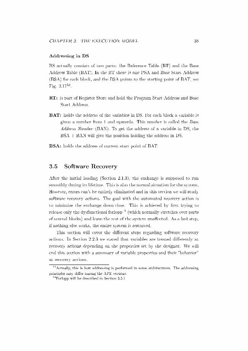
Addressing in DS
RS actually consists of two parts: the Reference Table (RT) and the Base
Address Table (BAT). In the RT there is one PSA and Base Start Address
(BSA) for each block, and the BSA points to the starting point of BAT, see
Fig. 3.1713.
RT: is part of Register Store and hold the Program Start Address and Base
Start Address.
BAT: holds the address of the variables in DS. For each block a variable is
given a number from 1 and upwards. This number is called the Base
Address Number (BAN). To get the address of a variable in DS, the
BSA + BAN will give the position holding the address in DS.
BSA: holds the address of current start point of BAT.
3.5 Software Recovery
After the initial loading (Section 2.1.3), the exchange is supposed to run
smoothly during its lifetime. This is also the normal situation for the system.
However, errors can't be entirely eliminated and in this section we will study
software recovery actions. The goal with the automated recovery action is
to minimize the exchange down-time. This is achieved by �rst trying to
release only the dysfunctional forlopp14 (which normally stretches over parts
of several blocks) and leave the rest of the system una�ected. As a last step,
if nothing else works, the entire system is restarted.
This section will cover the di�erent steps regarding software recovery
actions. In Section 2.2.3 we stated that variables are treated di�erently at
recovery actions depending on the properties set by the designer. We will
end this section with a summary of variable properties and their �behavior�
at recovery actions.
13Actually, this is how addressing is performed in some architectures. The addressing
principles may di�er among the APZ versions14Forlopp will be described in Section 3.5.1

CHAPTER 3. THE EXECUTION MODEL 39
PSA BSA
Base Address 1(the word-address of a
stored variable)Base Address 2
.....
Base Address n
BaseAddress
Table
ReferenceTable
PS
BN-R RS DS
1
2
3
Block ABlock B
Block n
.....
Block A
Block B.....
Block n
1 = BSA indicates the starting point of base address table for block A located in referencestore. The BSA will give the absolute address.2 = BAN indicates where the BAT word address for the specific variable is found. BAN is arelative address.3 = The word address indicates where the value of the specific variable is stored in DS.
Figure 3.17: Show how addressing to DS is performed in RS. BSA points to
the starting point of BAT

CHAPTER 3. THE EXECUTION MODEL 40
3.5.1 Forlopp
The �rst line of defense for maintaining system availability is the Forlopp
release. The purpose of a forlopp release is to allow a single process chain,
e.g., a call, to be released without adversely a�ecting any other processes in
the system.
Forlopp originates from the Swedish word �förlopp� meaning �sequence of
related events�. In the contents of AXE, a typical forlopp will result in a �path
through the system� which generally will be represented by a chain of linked
software resources, such as records. In AXE, the word forlopp can be used to
denote both the �sequence of related events� and the resulting �path through
the system�. The forlopp mechanism is implemented in the Maintenance
Subsystem, MAS, Fig. 2.1. Examples of forlopps are an ordinary telephone
call or a command. Some concepts associated with forlopps:
� A forlopp identity (FID), stored in a special register, is assigned to
each process (a call or forlopp). All parts participating in the same
forlopp have the same forlopp identity.
� The forlopp manager (FM) stores information concerning the di�erent
forlopps.
� When a software error is detected, the FM sends release signals to the
blocks involved according to the information stored in FM. A forlopp
release is hereby performed.
� At a forlopp release, a software error dump is performed, which means
that the contents of the records participating in the current forlopp are
dumped15.
To summarize, a detected software fault may result in a forlopp release, pro-
vided that the function block in which the fault occurred is forlopp-adapted
and the forlopp function is active.
3.5.2 System Restart
The system restart has been the traditional recovery action taken by the APZ
(Section 2.1) when it detects a software fault. The system restart a�ects the
15Section 2.1.3 describes what a dump is.

CHAPTER 3. THE EXECUTION MODEL 41
entire system and not only the forlopp in which the fault occurred. The
purpose of a system restart is to restore the system to a prede�ned state.
During restart, restart signals are sent to each block, so that during suc-
cessive restart phases, blocks perform actions to complete the initialization
or restoration to a consistent value of their data store variables.
The system restart procedure could be initiated manually, by a COMMAND
(Section 2.1.2), or automatically. A manual system restart clears error sit-
uations, for instance the disconnection of a hanging device. An automatic
system restart is detected by programs, microprograms and supervisory cir-
cuits. At a system restart, the job table, the job bu�ers and the time queues
(Section 3.3) are cleared.
There are three levels of system restart activities:
� Small system restart, which does not a�ect calls in speech position and
semi-permanent connections. Other calls are disconnected. This is a
minimal system restart.
� Large system restart in which all calls are disconnected. Semi-permanent
connections are not a�ected.
� Reload and large system restart in which a reload is performed �rst
to ensure that RELOAD-marked variables contain correct values. This is
then followed by a large system restart. Semi-permanent connections
are disconnected and automatically reestablished.
The reason to have di�erent types of system restarts is to disturb tra�c
handling as little as possible during the restart phase.
With the occurrence of the �rst fault in a normal block that leads to a
system restart, the system tries to repair itself without disturbing the tra�c
too much - A small system restart is initiated. If another serious fault occurs
within a prede�ned time interval, a large system restart will be initiated. In
the event of the occurrence of a third serious fault within another prede�ned
time interval, a reload and a large system restart will take place. This
represents the system's most extreme error-recovery action. The described
phases is pictured in Fig. 3.18.
Finally, it is sometimes unnecessary to immediately initiate an automatic
system restart. The system restart could be delayed or inhibited. This is
done by calling the selective restart function.

CHAPTER 3. THE EXECUTION MODEL 42
timex min x min
SmallRestart
SmallRestart
LargeRestart
Reload+
LargeRestart
Figure 3.18: Di�erent types of system restart.
3.5.3 Forlopp Release or a System Restart?
In Section 3.5.1 we described the concept of forlopps as a way to recover from
a software error without a�ecting more than the faulty forlopp. Then, in the
following Section, 3.5.2, we described the system restart and the di�erent
levels of restart and when they apply. This section explains when the system
restart action takes over from the forlopp release mechanism.
As we said in Section 3.5.1, a forlopp release is always a �rst choice if an
error has been detected. The system restart �function� applies when and if:
� The forlopp release fails to recover the system (i.e., the faulty forlopp),
or
� The faulty process has not been forlopp-adapted, or
� The number of faults have been to high according to a predetermined
limit.
The last case is checked against an intensity counter. This counter keeps
tracks of the quantity of software faults. The counter is stepped each time
a fault is detected leading to a delayed system restart or a forlopp release.
When the counter reaches the predetermined limit, a system restart is initi-
ated. The counter is then reset and starts again from zero. Fig. 3.19 shows
the intensity counter and Fig. 3.20 shows the di�erent levels of software
recovery.

CHAPTER 3. THE EXECUTION MODEL 43
time
Countervalue
Restart limit (default = 25)
+5
+10
+3
-1 every hour
No restartError is ignored
Delayedrestart
Forlopprelease
Figure 3.19: The intensity counter.
ERROR
Forlopp releasepossible and active?
SelectiveRestart active?
Intensitycounter high?
Check blockcategory
Error ignored
Delayed restart
Immediate restart
Delayed restart with reload
System Restart
0 1 2 3
Yes Forlopprelease
System Restart
No
No
No
Yes
Yes
Figure 3.20: Di�erent levels of recovery after a detected software error.

CHAPTER 3. THE EXECUTION MODEL 44
3.5.4 Variables and Software Recovery
As said in Section 2.2.3, the variable properties determine how the variables
are to be treated (i.e., from a data point of view) in the case of a system
restart. Fig. 3.21 shows the principles of how di�erent types of variables
should be treated after a system restart.
DS DS DUMP DS STATIC DS RELOAD DS RELOAD DUMP DS RELOAD STATIC
DS CLEAR DS CLEAR DUMP
StartSmall
system restartLarge
system restart
System restartwith
reloading Cannot be trusted
Cannot be trusted
Can be trusted Can betrusted
Can be trusted
Cannot be trusted Exception: when the variable value is checked in system restart routine
Figure 3.21: Data security of di�erent start/restart types.

Part II
Semantics
45

Chapter 4
Related Work
In Section 1.1, we mentioned that e�orts have been made to replace PLEX
with, or �map� PLEX to, speci�cation languages like SDL for instance. The
latest version of SDL (Speci�cation and Description Language), SDL2000,
has been given a formal (semantic) de�nition1. Work on this can be found
in [IT00] and [EGG+01]. Whether or not SDL and PLEX are �compatible�
with each other is still discussed within the PLEX design group, and will
not be a subject of study in this report.
Another language used for speci�cation is UML, Uni�ed Modeling Lan-
guage. The relation between PLEX and UML has been discussed in [AGG99].
A dialect of UML, UML-RT, is discussed by Herzberg in [Her99]. This paper
investigates the mapping between PLEX and UML-RT. This paper is pub-
lished within the E-CARES project2, which also explores the AXE system,
but from a �re-engineering� point of view.
Another language used in the same domain, i.e., the telecommunication
domain, is CHILL (CCITT High Level Language), which was developed by
the International Telecommunication Union (ITU), [IT99]. The language has
been speci�ed by the Vienna Development Method, [BJ82], in [IT82]. This
is a denotational framework and could be of interest since CHILL is used in
the same domain as PLEX. But, since the VDM is more of a speci�cation
method, that goes from abstract notation to formal speci�cation, whereas
1See the home page of the SDL Formal Semantics Project on:
http://rn.informatik.uni-kl.de/projects/sdl/2Home page:
http://www-i3.informatik.rwth-aachen.de/research/projects/ecares/Main.html
46

CHAPTER 4. RELATED WORK 47
this work goes from an implemented language to a formal speci�cation, the
VDM will not be considered in this report.
CHILL has also been covered by Winkler in [Win00].
Chapter 5
Programming Language
Semantics
What is programming language semantics and how/when is it used? The
�rst section in this chapter is devoted to answer these questions. We will
explain what we mean by a semantic description of a programming language.
The following sections will look at the most common forms of semantics.
5.1 The meaning of a program
Programming language semantics is concerned with rigorously specifying the
meaning, or the e�ect, of programs that are to be executed. By e�ect we
mean, for instance, the contents of the memory locations, which parts of the
program that is to be executed, or the behavior of the hardware a�ected by
the program. A semantic speci�cation captures these things in a formal way,
and later in this chapter we will study di�erent approaches to this formal
description.
Formal descriptions of programming languages are becoming more and
more popular, e.g. the BNF1 is used to specify the syntax of PLEX. The
problem is that a formal description of the syntax says nothing about the
meaning of the program since �syntax is concerned with the grammatical
structure of programs� whereas �semantics is concerned with the meaning of
grammatically correct programs� [NN92]. It is also possible to distinguish be-
1Backus-Naur Form
48

CHAPTER 5. PROGRAMMING LANGUAGE SEMANTICS 49
tween static and dynamic semantics [Mos01]. Static semantics corresponds
to the compile-time behavior of the program, the dynamic semantics hence
corresponds to the run-time behavior.
But now when we know what programming language semantics is, how
can we use it? We consult [NN92] for an answer to this question:
� The semantics can reveal ambiguities and complexities in what may
look as a clear documentation of the language (e.g. the language man-
ual).
� The semantics can also form the basis for implementation, analysis and
veri�cation.
Even with these obvious advantages with formal semantics, it is still widely
regarded as being of interest only to theoreticians [Mos01].
5.2 Semantic approaches
The formalizations of a programming language may di�er, i.e. the explana-
tions (or the meaning) can be formalized in di�erent ways. Most frameworks,
or approaches, can be classi�ed as one of the following three categories:
� Operational semantics - How to execute the program. The operational
approach(es) is (are) concerned with how the e�ect of the computations
is produced. The meaning is often speci�ed by an abstract machine
and/or a transition system.
� Denotational semantics - The e�ect of executing the program. Deno-
tational semantics, in contrast to operational semantics, is only con-
cerned with the e�ect of the computation, not how it is obtained.
Meanings are modeled by mathematical objects representing the e�ect
of executing the constructs.
� Axiomatic semantics - Partial correctness properties of the program.
The axiomatic approach is concentrated on speci�c properties of a
program. These properties are expressed as assertions. Axiomatic
semantics involves rules for checking these assertions. There may be
aspects of the executions that are ignored since only speci�c properties
are considered.

CHAPTER 5. PROGRAMMING LANGUAGE SEMANTICS 50
These di�erent categories will be further investigated/explained in their own
sections (5.4, 5.5 and 5.6), but we can already state that in the general case,
the semantics will tell us something about the relation between an initial
and a �nal state2.
5.3 Notation
In the following studies of the di�erent approaches, some �semantic� nota-
tions will be used3. These notations may seem unfamiliar to the reader and
we will summarize some basic notations here.
� By [x 7! 5] we mean the function that maps the symbol x to the
numerical value 5. I.e. x has the value 5.
� s0 = [x 7! 5] is called a state. The state s0 where x maps to 5. We
will also use the general form s x to denote the variable x in state s.
For a value 3, bound to x in the state s, we will write s x = 3.
� By hx := z; s0i ! s1 we mean that the execution of x:=z in the state
s0 will result in the new state s1.
� We will later talk about semantic functions and use the notation [[ ]]
to denote the syntactic argument (enclosed in syntactic brackets) to
the semantic function.
� We will use tt and � to denote the truth values true and false, re-
spectively.
�h S1; s i ! s0; h S2; s0 i ! s00
h S1; S2; si ! s00 is called a rule. It has a number of
premises above the solid line and one conclusion below the solid line.
A rule may also have a number of conditions that have to be ful�lled
whenever the rule is applied.
� We will use ) as the transition relation, i.e., when we go from one
state to another with the execution of one statement.
� )� means that we take zero or more steps from an initial to a �nal
state.
2The meaning of a state is explained in the following subsection.3The notation used in this report are the same as used in [NN92]

CHAPTER 5. PROGRAMMING LANGUAGE SEMANTICS 51
5.4 Operational Semantics
In Section 5.2 we said that a semantic formalism tells us something about
the relationship between the initial and the �nal state. In the Operational
approach we are not only interested in this relationship. We also want to
know how the computations that lead to the �nal state modify the interme-
diate state(s) as well. The di�erent operational approaches di�er in the level
of details:
� In the Natural semantics, the focus is on how the overall results of the
executions are obtained, whereas
� in the Structural operational semantics, it is of interest in how the
individual steps of the execution takes place4.
These two di�erent approaches will be studied in the following subsections
(5.4.1 and 5.4.2). For both styles of operational semantics, the meaning of
statements is speci�ed by a transition system with two di�erent con�gura-
tions:
� hS; si which means that the statement S is to be executed from the
state s.
� s that represent a terminal state, i.e. a termination of the computation.
5.4.1 Natural Semantics
The relationship between the initial and the �nal state of the execution of a
statement is in focus for the natural semantics (ns). The transition system
speci�es this relationship for every statement and is written in the form
hS; si ! s0 which, intuitively, means that the execution of the statement S
from state s will terminate and the resulting state will be s0. The execution
of the statement S on the state s will:
� terminate i�5 there is a state s0 such that hS; si ! s0, and provided
that the language under consideration is deterministic, or
4Natural semantics is also known as Big Steps Semantics, whereas the structural op-
erational approach sometimes is called Small Steps Semantics. These alternative names
tell us something about how detailed the transition is speci�ed.5if and only if

CHAPTER 5. PROGRAMMING LANGUAGE SEMANTICS 52
� loop i� there is no such state s0.
An example on how a natural semantics may look is given in Fig. 5.16. In this
table, we see a compound statement consisting of the individual statements
S1 and S2. We see that the execution of S1 from s results in a �nal state s0,
a �nal state that also is a start state in the con�guration h S2; s0 i which
has the �nal state s00. So, the execution of the compound statement S1; S2
from the start state s result in a �nal state s00.
[compns]h S1; s i ! s0; h S2; s0 i ! s00
h S1; S2; si ! s00
Figure 5.1: The compound statement expressed in natural semantics.
5.4.2 Structural Operational Semantics
In the natural semantics, we were interested in the relationship between the
initial and the �nal state when a statement was executed. In the structural
operational semantics (sos), we are also interested in the intermediate states
as well. I.e., if the execution of the statement S in state s leads to the �nal
state s0, the structural operational semantics will tell us something about the
intermediate states that are �visited� during the execution. In other words,
the focus is on the individual steps of the execution. The transition system
has the form hS; si ) where is either of the form hS0; s0i or of the form
s0. This means that the transition system expresses the �rst step of the
execution of the statement S from the state s and the result of this is .
� If is of the form hS0; s0i then the execution of S from s is not com-
pleted and the rest of the computation is expressed by the intermediate
con�guration hS0; s0i.
� If , on the other hand, is of the form s0, then the execution of S has
terminated and the �nal state is s0.
6This, and other examples of semantic styles/approaches in Section 5.2 are all from
[NN92].

CHAPTER 5. PROGRAMMING LANGUAGE SEMANTICS 53
In Fig. 5.2 we express the compound statement in a structural operational
semantics style. Unlike the natural semantics in Fig. 5.1, we see two �cases�
for the compound statement. In the �rst case, the execution is not completed
and the next con�guration (from hS1; si) is the intermediate con�guration
hS01; s0i. In the second case, the execution of S1 is completed and the �nal
state is s0. From this state, the execution of the con�guration hS2; s0i can
start.
[comp 1sos]
h S1; si ) h S0
1; s0 i
h S1; S2; s i ) h S0
1; S2; s0 i
[comp 2sos]
h S1; si ) s0
h S1; S2; s i ) h S2; s0 i
Figure 5.2: The compound statement expressed in structural operational se-
mantics.
5.5 Denotational Semantics
With the operational approach, the focus was on how the program was exe-
cuted - �How to compute.� In the denotational approach, the emphasis is on
�the e�ect of computing�. By e�ect, we mean the relationship between the
initial and the �nal state. The denotational approach consists of de�ning
semantic functions for each syntactic category. This semantic function maps
each syntactic construct to a mathematical object, most often a function,
that describes the e�ect of executing the construct. In Fig. 5.3, we see a
denotational description of the compound statement (previously shown in
Figure 5.1 and 5.2). In the Figure, we see that the e�ect of computing the
compound statement S1; S2 is the functional composition of executing S1
followed by S2.
5.6 Axiomatic Semantics
With the operational as well as the denotational approach, we are concerned
with the meaning of a given program. This is in contrast to the axiomatic

CHAPTER 5. PROGRAMMING LANGUAGE SEMANTICS 54
Sds[[S1; S2]] = Sds[[S2]] Æ Sds[[S1]]
Figure 5.3: The compound statement expressed in denotational semantics.
approach were we study properties of a given program. These properties
(expressed as assertions) could, for instance, be execution times (see [NN92]
for an example) or the degree of resource utilization. But, since the focus is
on speci�c properties and not on the meaning (as in the previously described
styles) �there may be aspects of the execution that are ignored� [NN92]. Ax-
iomatic de�nitions is often given in the form
fPgSfQg
where P is a Pre-condition, S the statement to be executed and Q a Post-
condition. This is to be interpreted as: �If P holds and the execution of S
terminates, then Q will hold�. In Fig. 5.4 we show the compound statement
in the axiomatic style. From this, we can say that if the pre-condition P
holds and the execution of S1 followed by the execution of S2 terminates
holds, then the post-condition R will hold.
Sp[[S1;S2]]fPgS1fQg; fQgS2fRg
fPg S1; S2 fRg
Figure 5.4: The compound statement expressed in a axiomatic semantics
style.

Chapter 6
Semantic Approach
6.1 Selected Approach and Motivation
In the process to determine a proper semantic approach for PLEX, it was
early agreed that the axiomatic approach (described in Section 5.6) was not
a suitable choice because of the rather abstract notation and also because its
focus is on properties more than the e�ect. So, the selection had to be made
between some form of operational semantics, or the denotational approach.
Some considerations that were taken into account:
� The operational semantics has its main advantages1 in the fact that it
is relatively easy to understand and also that the executional steps are
explicit. A possible disadvantage may be the fact that the approach is
tightly connected to how a statement is executed (i.e., it is closer to
the actual execution than the denotational approach).
� For the denotational approach, the advantage is that since mathemat-
ical objects are in focus, it abstracts away from how programs are ex-
ecuted. It can therefore be seen as the denotational approach provides
a more formal basis for reasoning about programs. The disadvantage
lays in the notation - Mathematical notation may �scare� the unfamiliar
reader.
[NN92] claims that the denotational approach may be preferred when reason-
ing about programs whereas the operational approach may be preferred when
1This is the authors opinion.
55

CHAPTER 6. SEMANTIC APPROACH 56
implementing the language. The decision to use an operational approach was
based on the following considerations:
� It was a pre-request that the notation would be relatively easy to un-
derstand even by a reader unfamiliar with semantic notation.
� The language PLEX is continuously updated and new hardware is
introduced in periodic intervals. This means that our semantic de-
scription also could be seen as a reference manual for new (future)
implementations of the language.
A second decision had to be made whether we should use the natural
semantics (described in Section 5.4.1) or the structural operational semantics
(described in Section 5.4.2). Even if the PLEX language does not provide
parallelism today, it is shown that many constructs are suitable for parallel
execution [Lin03], and to be able to deal with this in a future extension of
the (language and the) semantics, the structural operational approach were
preferred2.
6.2 The State of the System
In order to develop a semantic framework for PLEX, we have to determine
what a state of the system is since the execution of a statement will change
the current state, i.e., with the execution of a statement, we go from an old
state to a new state. Our starting point will be:
� With the state of the system, we mean the contents of the memory.
So, in order to determine the state of the system, we will look at the di�erent
forms of storage that exist in the system.
The �rst thing we have to consider is the memory and stores of the
Central Processor. The memory in the Central Processor (CP) consists of
the register memory and the di�erent stores.
The register memory is used for storing of temporary variables, pointers
and for transferring of signal data between di�erent �processes�3. Values in
2[NN92] shows why the structural operational semantics is well suited for parallel con-
structs.3The transferring of signal data have similarities to an ordinary function call: Just as
variables are loaded when the function is entered, are the signal data loaded at the start
of a sub-program, i.e., at a SIGNAL ENTRY.

CHAPTER 6. SEMANTIC APPROACH 57
the registers are lost after an EXIT from a job, or other register killing state-
ments such as direct signals, combined signals or IO statements, for example.
These are all statements that force the execution to leave the current block.
Temporary variables are only �alive� (i.e., containing a value in a register)
from the �rst write to it, until the last use. The PLEX compiler keeps track
of write-read chains and only allocates registers while the variables are alive
during the execution.
The di�erent stores in the CP were shown in Fig. 2.3. They are repeated
in Fig. 6.1. The di�erent forms of storage contains the following information:
� The Program Store is used for the storage of programs.
� Variables that is to survive the termination of a �process� or a system
restart, are stored in the Data Store.
� The Reference Store, �nally, contains information about where to �nd
the di�erent programs and data.
Program Store
PS
Reference Store
RS
Data Store
DS
Figure 6.1: The di�erent stores in the central processor (CP).
The second thing that is important, is the di�erent kind of job bu�ers (which
are used to store the di�erent kinds of signals). A simpli�ed �gure of the
job bu�ers is shown in Fig. 6.24. The semantics of the job bu�ers are the
FIFO5 approach, as shown in Fig. 6.3. Associated with each job bu�er
are two pointers, Job Bu�er In (JBI) and Job Bu�er Out (JBO). These
pointers make it possible for the APZ (the operating system) to know where,
in a job bu�er, to insert a signal that is to be bu�ered, or from where to fetch
a new signal. The memory layout, in a job bu�er, for one bu�ered signal
is pictured in Fig. 6.4. The job bu�er will consequently consist of several
items of the form described in the picture. So, as stated in the beginning of
4A more detailed description is found in Fig. 3.10.5First-In-First-Out

CHAPTER 6. SEMANTIC APPROACH 58
JBA - urgent tasks of the operating system; preferential traffic JBB - all other telephone traffic JBC - input/output to operator and I/O devices JBD - APZ routine self-tests JBR - Signals from Central Processor to Regional Processor
Job buffers for CP-CPand RP-CP signals
Job buffer for CP-RP signals
JBA
JBB
JBC
JBD
JBR
Figure 6.2: A simpli�ed �gure of the job bu�ers in the PLEX/AXE environ-
ment. (See also Fig. 3.10)
...Enter SigA
...
Unit B
Job Buffer...Send SigA
...EXIT
...
Unit A
JBI JBO
Figure 6.3: The FIFO-semantics of the job bu�ers.

CHAPTER 6. SEMANTIC APPROACH 59
W0
W1
W2
W3
W4
W5
W6
W7
W8
W9
W10
W11
Wn
IPOINTER LI
0 BN|R
0 BN|S
BN|S ND
FORLOPP ID B0 15
STYPE 0L F
FORLOPP ID B16 31TR
POINTER B0 15
POINTER B16 27
DATAWORD 0
DATAWORD 1
DATAWORD N
0 LSN (SNX)
LI - Lengt Indicator LSN - Local Signal Number. The entry point in the Signal Distribution Table of the receiving block DATAWORD <p> - Where the actual data is placed
Figure 6.4: Organization of the job bu�ers. NOTE: The pointer registers,
W8-W9, are treated as one register (and referred to as POINTER B0). This
is due to the fact that the register in W9 is only used when a pointer is too
large to �t only in W8. In this case, the pointer will be split up and placed
in W8 with its �rst half, and in W9 with its second half.

CHAPTER 6. SEMANTIC APPROACH 60
this section, our starting point in determining the state of the system, was:
� With the state of the system, we mean the contents of the memory.
And, we can now tell that the contents of the memory is the contents of the
register memory, the contents of the di�erent stores, and the contents of the
job bu�ers. The state of the system can, at this point, be represented as a
tuple of the form6:
hRM;PS;DS;RS; JBA; JBB; JBC; JBD; JBRi
where RM = Register Memory, PS = Program Store, DS = Data Store, RS
= Reference Store, JBA = Job Bu�er A, JBB = Job Bu�er B, JBC = Job
Bu�er C, JBD = Job Bu�er D and JBR = Job Bu�er R.
The above representation would indeed be su�cient if PLEX was a
strictly sequential language, i.e., if statementA precedes statementB in our
source code �le, then we could be absolutely certain that statementA would
execute before statementB. This holds in a language without the possibility
to manipulate the Program Counter, e.g., with a JUMP statement. But since
these kind of statements do exist in PLEX7, we also have to model the pos-
sibility of �moving� the execution to somewhere di�erent from the following
statement. If we had been dealing with some kind of assembler code, the
above could easily be managed by adjusting the Program Counter according
to the instructions executed by the CPU. But we are not looking at the se-
mantics from an instruction level point of view, instead we are working with
statements that consists of n instructions.
� Our solution is to de�ne the Virtual Statement Counter, VSC
The VSC contains an address (an integer value), which tells where the �rst
instruction in the next statement resides in memory. By stepping up the
VSC with 1, we step it up to the �rst instruction in the next statement8.
If nothing else is stated, the VSC will always be stepped up to the next
6The contents of the memory could also be extended with the contents of the DATA
SECTOR (see Section 2.2.1), which is used in a startup phase as well as in a system restart
phase. But since we do not cover those phases in this report, the contents of the Data
Sector is omitted in our description of the systems state.7E.g., the GOTO statement.8The approach is similar to the one described in [Lis98], where the program counter is
modi�ed in a similar way.

CHAPTER 6. SEMANTIC APPROACH 61
statement after the execution of a previous statement, i.e., s[VSC 7! VSC+1].
For convenience, we will use the notation s[VSC++] to denote s[VSC 7!
VSC+1]. In situations where this is obvious, we will omit this �information�.
A situation where this is the case would for instance look like: hS1; si )
hS0
; s0
i
The above leads us to the following de�nition of the state of the system:
hVSC; RM;PS;DS;RS; JBA; JBB; JBC; JBD; JBRi
6.3 Lexical Units and Syntactical Categories
In this section9, we will follow the conventions in [AB02] and use the same
variant of EBNF (Extended Backus-Naur Form) notation.
� ::= is used as the �de�nition operator�.
� We will mark a KEYWORD with bold, upper case letters.
� The vertical bar, |, represents a choice between elements.
� The square brackets [ ] are used to denote an optional construct. I.e.,
the construct inside the brackets may be omitted.
� Optional properties are marked in a separate way, like in �length�.
� Curly brackets, f g, are used to delimit an operand, or simply to im-
prove readability. f g� represents a possibly empty sequence of ele-
ments, i.e., the element may be repeated zero or more times. Finally,
f g+, are used for the non-empty sequence of elements.
The lexical units and the syntactic categories10 in PLEX are as follows:
� upper-case-letter ::= A|B|C|...|X|Y|Z
� lower-case-letter ::= a|b|c|...|x|y|z
� letter ::= upper-case-letter | lower-case-letter
� decimal-digit ::= 1|2|3|...|7|8|9
� hexadecimal-digit ::= 1|2|...|8|9|A|B|...|E|F
9The syntactical material in this section is basically compiled together from the fol-
lowing internal Ericsson documents: [AB98, AB02, AB86]10Please note that the syntactical categories in this section are only a subset of the
language.

CHAPTER 6. SEMANTIC APPROACH 62
� special-character ::= !|"|#|%|1|'|?|(|)|*|+|,|-|.|/|:|;|<|=|>|_
|[|]|$|@
� character ::= letter | decimal-digit | special-character
� identi�er ::= letter fletter | decimal-digit | _f letter | decimal-digitgg�
� decimal-numeral ::= decimal-digitfdecimal-digit | _g�
� hexadecimal-numeral ::= hexadecimal-digitfhexadecimal-digit | _g�
� numeral ::= [+]fdecimal-numeral | hexadecimal-numeralg
� string-object ::= �characterfcharacterg��
� arithmetic-operator ::= '+' | '-' | '*' | '/'
� bit-operator ::= '(-)' | '(*)' | '(+)' | '(=)' | '=>' | '<='
� relation-operator ::= '<' | '=<' | '=' | '/=' | '>=' | '>'
� binary-operator11 ::= arithmetic-operator | bit-operator12 | relation-operator
y There are no syntactic categories such as arithmetic or boolean expres-
sions in PLEX. Instead, there is the �eld-expression. A �eld expression
is one or several operands separated by arithmetic or �logical�13 opera-
tors14. We could say, �separated by binary operators�, but that would
include bit operators that don't �give� logical values.
Field expression is evaluated from left to right and according to the
priorities shown in Table 6.1.
� �eld-expression ::= [+|-] sub-expression
� subexpression ::= operand | negation-operator sub-expression
| subexpression binary-operator subexpression
| '('subexpression')'
� operand ::= �eld-variable | pointer | numeral | number-symbol
yOperands and (sub)expressions can only adopt positive integers [AB02]!
� �eld-variable ::= identi�er
y When a �eld-variable is declared, the variable properties must also be
speci�ed. The variable properties is concerned with if the variable is
stored or temporary, and how the variable is to be treated during
11The meaning of, and the priority among the operators are summarized in Table. 6.1.12All bit operators are binary operators except the NOT-operator '(-)'.13With logical operators, we mean operators that are used in expressions that we think
of as being true or false, and these operators are marked as logical in Table 6.1.14I.e., arithmetic and boolean expressions exist, but are both called �eld expressions.

CHAPTER 6. SEMANTIC APPROACH 63
software recovery actions. The property is speci�ed as a valid15 combi-
nation of the keywords: DS,BUFFER,COMMUNICATION BUF-
FER, CLEAR, SEMICLEAR, RELOAD, DUMP, STATIC and
TRANSIENT
� pointer ::= POINTER pointer-name '('record-name')' ';'
� pointer-name ::= identi�er
� record-name ::= identi�er
y [AB98] states that the pointer-name should end with the su�x pointer,
ptr or p.
yy Pointers are not more than record numbers (i.e., positive integers). A
pointer is always associated with a �le and the value of the pointer is
the number of the current record in that �le. (See Section 2.2.2 for
details.)
yyy Pointers behave like, and are treated as, temporary variables. I.e.,
pointers are stored in the register memory and they may loose their
value whenever the execution of the software unit terminates.
There is no explicit pointer arithmetic, instead they are treated and
used as operands in �eld-expressions (described above) and in assign-
ment statements (described later in this section).
� number-symbol ::= identi�er
y Number symbols have the same semantic meaning as constants in C (for
example).
yy Number symbols are declared in the Declare Sector (see Section 2.2.1)
with the statement:
NSYMB identi�er '=' fdecimal-numeral | hexadecimal-numeralg';'
� condition ::= �eld-expression relation-operator �eld-expression
| symbol-variable ['=' | '/='] symbol-value
| string-object ['=' | '/='] string-object
� symbol-variable ::= SYMBOL VARIABLE
'('symbol-value f; symbol-valueg�')' [properties] ';'
� symbol-value ::= identi�er
� properties = A valid combination of: DS, BUFFER, COMMUNI-
15The valid combinations of the variable properties, as well as the meaning of the dif-
ferent properties is covered in Section 2.2.3.

CHAPTER 6. SEMANTIC APPROACH 64
CATION BUFFER, CLEAR, SEMICLEAR, RELOAD,
DUMP, STATIC and TRANSIENT
y Symbol variables are also known as enumeration type variables, a con-
cept that is familiar to C programmers. Their use is to hold symbol val-
ues, which in the AXE domain could be IDLE, BUSY, BLOCKED for inst-
ance. A symbol variables can be assigned symbol values and compared
to other symbol variables.
yy The code generation phase16 replaces the symbol values with numeri-
cal values. This is why symbol variables can be assigned to, and com-
pared with, �eld variables (that store numerical values). I.e., if a �eld
variable is assigned a symbol value, the numerical value of the symbol
is assigned the �eld variable.
Priority Operator Meaning Type
1 (-) Logical NOT Bit operator (logical)
2 => Shift right Bit operator
2 <= Shift left Bit operator
3 * Multiplication Arithmetic
3 / Division Arithmetic
4 +, - Addition, Subtraction Arithmetic
5 = Equality Relation (logical)
5 /= Inequality Relation (logical)
5 < Less than Relation (logical)
5 > Greater than Relation (logical)
5 =< Less or equal than Relation (logical)
5 >= Equal or greater than Relation (logical)
6 (*) Logical AND Bit operator (logical)
7 (=) Logical XOR (Exclusive or) Bit operator (logical)
8 (+) Logical OR Bit operator (logical)
Table 6.1: Priorities and meaning of the PLEX operators. Priorities are
numbered from the highest (1) to the lowest (8).
16The code generation phase is the process of translating (in several steps) the source
code (PLEX) to machine code. (The compilation process, in which the code generation
takes place, is covered in [AE00].)

CHAPTER 6. SEMANTIC APPROACH 65
6.4 Statements for Variable Assignments
The general form of the assignment statement has the following syntax:
� assignment-statement ::= [SET] variable '=' expression ';'
We recall (from Section 2.2.3) that PLEX have three di�erent types of vari-
ables; Field variables for numerical information, symbol variables for sym-
bolic values, e.g., IDLE, BLOCKED, BUSY, etc and string variables which store
text strings. This implies the following three statements for variable assign-
ment:
� �eld-assignment-statement ::= [SET]
f f fpointer | �eld-variableg '=' g+
f�eld-expression | maxnum-expressiong g
| f �eld-variable '='g+ symbol-variable ';'
� maxnum-expression ::= MAXNUM OF variable
y The value of a maxnum-expression is the number of individuals in
the �le associated with the given variable name.
� symbol-assignment-statement ::=
[SET] fsymbol-variable '='g+ symbol-value ';'
� string-assignment-statement ::=
[SET] fstring-variable '='g+ string-object ';'
6.5 Jump Statements
PLEX o�ers both conditional and unconditional jump statements. The �pro-
grammer guidelines� for the use of jump statements are: �Please avoid back-
ward jumps as far as possible, because they are di�cult to follow.� and �Try to
avoid jump statements, since they can give rise to a poor program structure.
It is very di�cult to read a program with a great many jump statements.�
[AB98]. But still, they are part of the language, and we will look at their
syntax here.
The unconditional jump statement simply interrupts the sequential exe-
cution order and its syntax is as follows:

CHAPTER 6. SEMANTIC APPROACH 66
� unconditional-jump-statement ::= fGOTO | GO TOg label ';'
The conditional jump statement o�ers a possibility to jump if the given con-
dition is met. It has the form of an if-statement with a goto:
� if-statement ::= IF [NOT] condition [PROCEED ELSE]
fGOTO | GO TOg label ';'
Since condition will return in other statements, its syntax is given here:
� condition ::= f�eld-expression1 relation-operator �eld-expression2g
| fsymbol-variable f'=' | '/='g symbol-valueg
| fstring-object f'=' | '/='g string-object g
In connection to the jump statements, there is also the BRANCH statement
which selects between a number of program sequences, but since this state-
ment has been �removed�17 from the language, we will not cover it here.
6.6 Conditional Statements
The if-statement in Section 6.5 is a rather primitive construction since it
does not have an else clause and because the only permitted action is an
unconditional jump. This is the motivation for the following more recent
statement:
� improved-if-statement ::=
IF [NOT] condition THEN sequence-of-statements
fELSEIF [NOT] condition THEN sequence-of-statementsg�
[ELSE sequence-of-statements]
FI
17I.e., it is an old statement and should be avoided in new design [AB98].

CHAPTER 6. SEMANTIC APPROACH 67
6.7 Selections
The CASE statement is used for selection between an arbitrary18 number of
unambiguous choices:
� case-statement ::=
CASE expression IS
fWHEN choice f',' choiceg� DO sequence-of-statementsg+
OTHERWISE DO sequence-of-statements
ESAC ';'
� expression ::= �eld-expression | symbol-variable | string-object
� choice ::= numeral | number-symbol | symbol-value | string-symbol
| text-string
It is not allowed to use a signal reception statement (Section 6.9) inside the
sequence of statements part19. Neither is it allowed to jump into a CASE
statement.
6.8 Iterations
The well known While statement is missing in PLEX. The main reason is
that such a construct is not considered necessary in the application domain
(which is the central part of the AXE switching system). A second reason is
that the construct may give rise to unpredictable execution times, which is
not the case with the iteration statements in PLEX (see below).
Instead, PLEX o�ers three di�erent statements for iteration: ON, FOR
ALL and FOR FIRST. They are all used for scanning �les or indexed variables
between given start and stop values. The three iteration statements are
compared in Fig. 6.5 and their syntax are as follows:
� on-statement ::=
ON fpointer | �eld-variableg FROM �eld-expression
fUPTO | DOWNTOg �eld-expression
DO sequence-of-statements
NO ';'
18I.e., one or more19Which also holds for iterations and conditionals.

CHAPTER 6. SEMANTIC APPROACH 68
� for-statement ::=
FOR fFIRST | ALLg fpointer | �eld-variableg
FROM �eld-expression-1 [UNTIL �eld-expression-2 ]
[WHERE f [NOT] condition
| �eld-variable IS CHANGED TO �eld-expressiong]
f fGOTO | GO TOg label
| DO fstatement | statement-block-nameg g ';'
Criterion ON FOR ALL FOR FIRST
Ascending or descending order Yes Always descending
Several statements in action part Yes No, except in statement
blocks, IF, CASE and
loop statements
Condition in iteration statements NO Possible Always
Iteration ends after matching
condition once and handling one
individual
Not applicable No Yes
Iteration variable/pointer after
loop
Unde�ned Unde�ned De�ned if
matching
individ-
ual/condition
Generates high-speed loop No20 Possible Possible
Figure 6.5: PLEX iteration statements - a comparison.
6.9 Signal Sending/Receiving Statements
In Section 3.2 it was stated that the main distinction to be made between
the di�erent kinds of signals in PLEX is between direct and bu�ered signals.
And this is true from the point of view of the execution model, but from a
syntactical point of view, the main distinction is between single and combined
signals. Every signal will fall into one of these categories. I.e., from the
syntactical point of view it is only of interest whether one has to wait for an
�answer� (a combined signal) or not - Whether the signal is direct or bu�ered,
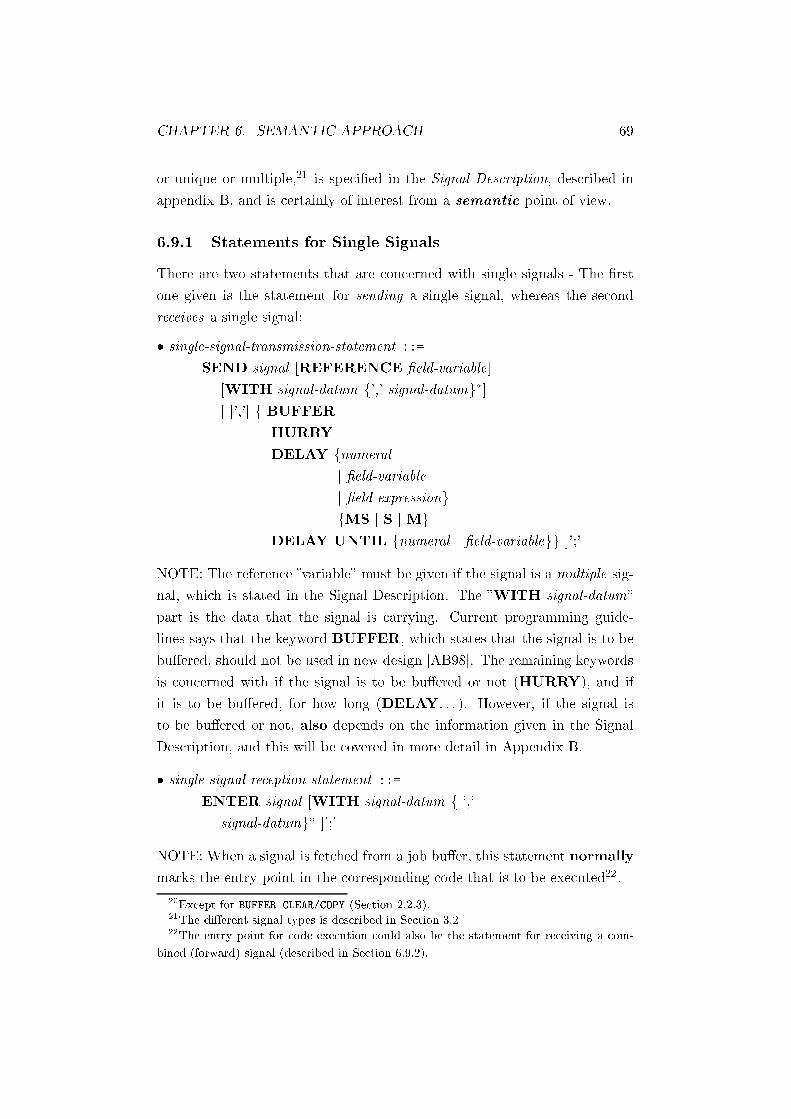
CHAPTER 6. SEMANTIC APPROACH 69
or unique or multiple,21 is speci�ed in the Signal Description, described in
appendix B, and is certainly of interest from a semantic point of view.
6.9.1 Statements for Single Signals
There are two statements that are concerned with single signals - The �rst
one given is the statement for sending a single signal, whereas the second
receives a single signal:
� single-signal-transmission-statement ::=
SEND signal [REFERENCE �eld-variable]
[WITH signal-datum f',' signal-datumg�]
[ [','] f BUFFER
| HURRY
| DELAY fnumeral
| �eld-variable
| �eld-expressiong
fMS | S | Mg
| DELAY UNTIL fnumeral | �eld-variablegg ]';'
NOTE: The reference �variable� must be given if the signal is a multiple sig-
nal, which is stated in the Signal Description. The �WITH signal-datum�
part is the data that the signal is carrying. Current programming guide-
lines says that the keyword BUFFER, which states that the signal is to be
bu�ered, should not be used in new design [AB98]. The remaining keywords
is concerned with if the signal is to be bu�ered or not (HURRY), and if
it is to be bu�ered, for how long (DELAY. . . ). However, if the signal is
to be bu�ered or not, also depends on the information given in the Signal
Description, and this will be covered in more detail in Appendix B.
� single-signal-reception-statement ::=
ENTER signal [WITH signal-datum f ','
signal-datumg� ]';'
NOTE: When a signal is fetched from a job bu�er, this statement normally
marks the entry point in the corresponding code that is to be executed22.
20Except for BUFFER CLEAR/COPY (Section 2.2.3).21The di�erent signal types is described in Section 3.222The entry point for code execution could also be the statement for receiving a com-
bined (forward) signal (described in Section 6.9.2).

CHAPTER 6. SEMANTIC APPROACH 70
6.9.2 Statements for Combined Signals
� combined-forward-signal-transmission-statement ::=
SEND cfsignal [REFERENCE �eld-variable]
[WITH signal-datum f',' signal-datumg�]
[',']
WAIT FOR cbsignal1 IN label
fOR cbsignaln IN labelg� ';'
NOTE: As could be seen in the syntax for the sending of a combined forward
signal, it must be speci�ed where (in the code) the �answer� is supposed to
arrive. Also, note that it is allowed to wait for more than one backward
signal. This is useful when one wants to take action according to the result
of the execution in the block that received the forward signal (and then sent
the backward signal).
The following statement is used for receiving of a forward signal.
� combined-forward-signal-reception-statement ::=
RECEIVE cfsignal
[WITH signal-datum f',' signal-datum g�] ';'
The following two statements is concerned with the answer to the initiating
part. The �rst statement is sending the �reply� whereas the second receives
the �answer�.
� combined-backward-signal-transmission-statement ::=
RETURN cbsignal
[WITH signal-datum f',' signal-datumg�] ';'
� combined-backward-signal-reception-statement ::=
label ')' RETRIEVE cbsignal
[WITH signal-datum f',' signal-datumg�] ';'
6.9.3 Statements for Local Signals
The following statements is for the sending, and receiving of a local signal,
respectively. (Local signals are described in Section 3.2.4.)
� local-signal-sending-statement ::=
TRANSFER signal

CHAPTER 6. SEMANTIC APPROACH 71
[WITH signal-datum f',' signal-datumg�] ';'
� local-signal-receiving-statement ::=
ENTRANCE signal
[WITH signal-datum f',' signal-datumg�] ';'
6.10 Exit
The exit statement is a deactivation statement for the sequence of statements
that begins with a signal reception statement for a single signal or a command
reception statement.
� exit-statement ::= EXIT ';'
NOTE: The exit statement marks the (possible) termination of a subprogram
and also the termination of a job, since the control is transferred back to the
operating system (which fetches the next job from the job bu�ers).
6.11 Semantic Functions
In order to develop a semantic description of the most important parts of
PLEX, which is considered to be the concept of signals (as mentioned in
Section 1.2), we need some semantic functions 23 24 that will help us ex-
pressing the meaning of the language. Some of them will be de�ned in this
section whereas the other will be de�ned when the need arise. However, we
summarize all semantic functions, that we de�ne and use in Chapter 6, in
Table 6.2.
The �rst function that we introduce is the function that determine the
number represented by a numeral, and this function is de�ned in the following
way:
N : numeral! Z
This function is to be read as �The semantic function N that takes a nu-
meral as input and returns the corresponding integer value�, i.e., a number.
23Semantic functions are brie�y introduced in Section 5.3.24When we, in this section as well as in the following report, denote the state of the
system with s, we mean the tuple hVSC; RM;PS;DS; RS; JBA; JBB; JBC; JBD; JBRi
that was speci�ed in Section 6.2.

CHAPTER 6. SEMANTIC APPROACH 72
Function De�ned in
N : numeral! Z Section 6.11
ST : string ! Characters Section 6.11
A : field-expression! Z Table 6.3, Section 6.11
B : field-expression! ftt, �g Table 6.4, Section 6.11
P : variable! var-property Section 6.11
ADR : label! Z Section 6.11
STMT : address! statement Section 6.11
SD : signal! sig-property Section 6.17
SIG : signal! address Section 6.17
L : signal! level Section 6.17
BLOCK : address! CodeBlock Section 6.17.2
APZ : state ,! state Table 6.5, Section 6.18
CODE : address! code Section 6.19
SPLEX : Code! state Section 6.19
Table 6.2: A summary of the semantic functions de�ned and used in Chapter
6 (and in Appendix A).

CHAPTER 6. SEMANTIC APPROACH 73
An example of applying the function is N [[137]] = 137 2 Z. NOTE: It is
important to understand the di�erence between the numeral 137, which is
a syntactic construct (and therefore enclosed in syntactical braces), and the
meaning of the numeral, which is the number 137. In the following, we will
write N [[n]] to denote the �meaning� of n, i.e., the corresponding numerical
value.
The second function is similar to the �rst, but �operates� on strings:
ST : string ! Characters
and returns the meaning of a string-object as in:
ST [[abc]] = abc 2 Characters
In other words, both N and ST captures what we intuitively think of when
we talk about the meaning of syntactical constructs such as '137' or 'abc'.
The third function we will use, is the function that will determine the
meaning of a �eld expression. We recall, from Section 6.3, that PLEX does
not contain the �usual� arithmetic and boolean expressions. Instead, there
is the �eld expression. But depending on the operator, the value of a �eld
expression could be seen as numerical or logical. We will therefore de�ne
two semantic functions for �eld expressions, one that applies when the ex-
pression is to be treated as an arithmetic expression, and one that applies
when the expression is to be treated as a logical expression. The �rst func-
tion, A, summarized in table 6.3, is de�ned in the following way:
� The meaning of a �eld expression, when the expression is a numeral as
in A[[n]]s, is given by the function N , as speci�ed above25.
� The meaning of a variable x is the value currently bound to the variable,
s x.
� The meaning of a �eld expression consisting of sub-expressions, A[[a1+a2]]s,
is determined by the meanings of the sub-expressions.
For �eld expressions that is to be treated as logical expressions, their seman-
tics is given by the semantic function B as speci�ed in Table 6.426.
25Remember that the s after the syntactic braces, [[ ]], represent the state of the system
which was speci�ed in Section 6.2.26When specifying the semantics for the Selection statement (Section 6.15), we will have
to compare two strings and see if they are equal. This motivates the rule B[[t1 = t2]]s in
the table.

CHAPTER 6. SEMANTIC APPROACH 74
A[[n]]s = N [[n]]
A[[x]]s = s x
A[[a1 + a2]]s = A[[a1]]s+A[[a2]]s
A[[a1 � a2]]s = A[[a1]]s�A[[a2]]s
A[[a1 � a2]]s = A[[a1]]s � A[[a2]]s
A[[a1 = a2]]s = A[[a1]]s = A[[a2]]s
Table 6.3: The semantics of �arithmetic� expressions.
The next function de�ned, is the function P, which will �nd the speci�ed
properties for the given variable. P is de�ned in the following way:
P : variable! var-property
where var-property � f";DS,BUFFER,COMMUNICATION BUFFER,
CLEAR, SEMICLEAR, RELOAD, DUMP, STATIC and TRAN-
SIENTg27.
It is necessary to determine the variable properties, since depending on which
properties that are speci�ed for the given variable, di�erent parts of the state
of the system will be updated in an assignment.
Finally, to be able to determine the start address for a given program
label and also to �nd the statement that is located at a given address, we
de�ne the following two functions
ADR : label ! Z
STMT : address! statement
where ADR takes a program label and returns its corresponding address,
and whereas STMT takes an address and returns the corresponding PLEX
statement.
27" is returned if the variable is temporary.

CHAPTER 6. SEMANTIC APPROACH 75
B[[a1 < a2]]s =
(tt if A[[a1]]s < A[[a2]]s
� if A[[a1]]s >= A[[a2]]s
B[[a1 =< a2]]s =
(tt if A[[a1]]s =< A[[a2]]s
� if A[[a1]]s > A[[a2]]s
B[[a1 = a2]]s =
(tt if A[[a1]]s = A[[a2]]s
� if A[[a1]]s 6= A[[a2]]s
B[[t1 = t2]]s =
(tt if ST [[t1]]s = ST [[t2]]s
� if ST [[t1]]s 6= ST [[t2]]s
B[[a1= = a2]]s =
(tt if A[[a1]]s 6= A[[a2]]s
� if A[[a1]]s = A[[a2]]s
B[[a1 >= a2]]s =
(tt if A[[a1]]s >= A[[a2]]s
� if A[[a1]]s < A[[a2]]s
B[[a1 > a2]]s =
(tt if A[[a1]]s > A[[a2]]s
� if A[[a1]]s =< A[[a2]]s
B[[(�)a1]]s =
(tt if B[[a1]]s = �
� if B[[a1]]s = tt
B[[a1(�)a2]]s =
(tt if B[[a1]]s = tt and B[[a2]]s = tt
� if B[[a1]]s = � or B[[a2]]s = �
B[[a1(=)a2]]28s =
8>><>>:tt if B[[a1]]s = tt and B[[a2]]s = �
tt if B[[a1]]s = � and B[[a2]]s = tt
� if B[[a1]]s = B[[a2]]s
B[[a1(+)a2]]s =
(tt if B[[a1]]s = tt or B[[a2]]s = tt
� if B[[a1]]s = � and B[[a2]]s = �
Table 6.4: The semantics of �boolean� expressions. (See also, Table 6.1 where
the di�erent operators, as well as their meaning, are described.) an represents
a �eld-expression whereas tn represents a string.

CHAPTER 6. SEMANTIC APPROACH 76
6.12 The Semantics for Assignment Statements
Now, when the required functions have been speci�ed, we are ready to ap-
proach the language constructs that is to be treated in this report. We start
with the semantics of the assignment statements, since these are the state-
ments that most obviously a�ect the state of the system by their change of
the contents in the memory.
First, from Section 2.2.3, we recall that from a storage point of view, the
main distinction to be made between variables is whether they are temporary
or stored which means that they reside in the register memory (RM) or the
data store (DS), respectively. To determine this, we use the function
P : variable! var-property
which was speci�ed last in the previous section. As was mentioned earlier
(Section 6.11) we will use s to denote the tuple
hVSC; RM;PS;DS;RS; JBA; JBB; JBC; JBD; JBRi
and if one item of this tuple is to be updated, we will write (DS)x if x in
the DS is to be updated. We will also use the notation RM 7! UNDEF in
situations where the contents of the register memory should be considered as
non-existing29. Secondly, we have three di�erent kinds of variables to deal
with; �eld variables, symbol variables and string variables. The semantics
for �eld variable and symbol variable assignments are similar, but we write
them as separate rules to make it explicit which kind of assignment we are
dealing with. This leads us to the following rules for assignment statements.:
� [assfield] hx := a; si ) s[VSC++; (DS)x 7! A[[a]]s] if P[[x]] = DS
� [assfield] hx := a; si ) s[VSC++; (RM)x 7! A[[a]]s] if P[[x]] = "
� [asssym] hx := a; si ) s[VSC++; (DS)x 7! A[[a]]s] if P[[x]] = DS
� [asssym] hx := a; si ) s[VSC++; (RM)x 7! A[[a]]s] if P[[x]] = "
The �nal assignment statement concerns string variables and for these, we
specify the following rules:
� [assstring] hx := c; si ) s[VSC++; (DS)x 7! ST [[c]]s] if P[[x]] = DS
� [assstring] hx := c; si ) s[VSC++; (RM)x 7! ST [[c]]s] if P[[x]] = "
28This rule could also be expressed as: B[[a1(=)a2]]s =
�tt if B[[a1]]s 6= B[[a2]]s
� if B[[a1]]s = B[[a2]]s29I.e., we use our own de�ned constant UNDEF in a way similar to the use of NULL in C.

CHAPTER 6. SEMANTIC APPROACH 77
6.13 The semantics for Jump statements
As mentioned in Section 6.5, PLEX o�ers two kinds of jump statements; Un-
conditional and conditional. The unconditional jump statement will always
perform a jump to the speci�ed label, whereas the conditional is dependent
on the evaluation of the given condition. Their respective semantics are as
follows:
� [jumpuncond] hGOTO label; si ) s[VSC 7! ADR[[label]] ]
� [jumpcond] hIF condition GOTO label; si ) s[VSC 7! ADR[[label]] ]
if B[[condition]]s = tt
� [jumpcond] hIF condition GOTO label; si ) s[VSC++]
if B[[condition]]s = �
6.14 The semantics for Conditional statements
We begin this section by repeating the syntax for the if-statement from
Section 6.6. This statement is denoted as the improved-if-statement since
it improves the above conditional jump statement. As could be seen, from
the syntax, the elseif as well as the else clause are optional. This will be
explicit in the semantics for the if-statement.
� improved-if-statement ::=
IF [NOT] condition THEN sequence-of-statements
fELSEIF [NOT] condition THEN sequence-of-statementsg�
[ELSE sequence-of-statements]
FI
� [condif ] hIF condition THEN S1; si ) hS1; si
if B[[condition]]s = tt
� [condif ] hIF condition THEN S1; si ) s[VSC++]
if B[[condition]]s = �
� [condif ] hIF condition THEN S1 ELSE S2; si ) hS1; si
if B[[condition]]s = tt
� [condif ] hIF condition THEN S1 ELSE S2; si ) hS2; si
if B[[condition]]s = �

CHAPTER 6. SEMANTIC APPROACH 78
The case IF...ELSEIF...ELSE can be seen as an instance of the IF...ELSE
rule and is therefore omitted.
6.15 The semantics for Selection statements
The syntax for the selection statement, CASE, was discussed in Section 6.7
and is repeated below:
� case-statement ::=
CASE expression IS
fWHEN choice f',' choiceg� DO sequence-of-statementsg+
OTHERWISE DO sequence-of-statements
ESAC ';'
The pair, expression/choice, is either numerical or strings. Both cases are
covered by B[[expression = choice]]s as could be seen from Table 6.4.
We give the semantics in term of the �basic case�, i.e., when CASE is
followed by one WHEN DO and terminated by a OTHERWISE DO. Multiple
instances of WHEN DO could be seen as instances of the �basic case�.
� [select] hCASE expression IS WHEN choice DO S1
OTHERWISE DO Sn; si ) hS1; si
if B[[expression = choice]]s = tt
� [select] hCASE expression IS WHEN choice DO S1
OTHERWISE DO Sn; si ) hSn; si
if B[[expression = choice]]s = �
6.16 The semantics for Iteration statements
As stated in Section 6.8, PLEX o�ers three di�erent statements for itera-
tions; Namely ON, FOR ALL and FOR FIRST. We will give their semantics30 in
turn.31
30Note: PLEX �o�ers� the possibility to jump out of an iteration with a GOTO statement
for example. This means that a proper semantics could not rely on a sequential execution
order! However, the following rules does not take that into consideration. I.e., the following
rules are speci�ed for well formed iterations, which consequently are iterations without
such jumps.31For convenience we use point/var for pointer/variable and expn for expressionn .

CHAPTER 6. SEMANTIC APPROACH 79
� [ONUp]
hS; si ) s0; hON point=var FROM exp1+1 UPTO exp2 DO S; s0i) s00
hON point=var FROM exp1 UPTO exp2 DO S; si ) s00
if A[[exp1]]s < A[[exp2]]s
� [ONUp] hON pointer/variable FROM 'expression1' UPTO
'expression2' DO S; si ) s[VSC++]
if A[[expression1]]s > A[[expression2]]s
The semantics for the ON-statement in the case of DOWNTO instead of
UPTO is almost the same in every step, as could be seen in the following
rules:
� [ONDown]
hS; si ) s0; hON point=var FROM exp1�1 DOWNTO exp2 DO S; s0i) s00
hON point=var FROM exp1 DOWNTO exp2 DO S; si ) s00
if A[[exp1]]s > A[[exp2]]s
� [ONDown] hON pointer/variable FROM 'expression1' DOWNTO
'expression2' DO S; si ) s[VSC++]
if A[[expression1]]s < A[[expression2]]s
Then follows the two FOR-statements, and we start with the FOR ALL. As
could be seen from the syntax for the FOR ALL statements (Section 6.8),
there are a lot of things that are optional. We omit these parts here. The
reason is that these parts only makes it possible to give more precise values
for the iteration variables. In its basic form (which will be the form we spec-
ify the semantics for), the FOR ALL statements iterate from pointer/�eld-
expression1 down to zero.
� [FORALL]32
hS; si ) s0;
hFOR ALL pointer=field-var FROM field-exp1 - 1 DO S; s0i ) s00
hFOR ALL pointer=field-var FROM field-exp1 DO S; si ) s00
if A[[field� exp1]]s > 0
32Due to space limitations, we will write only S where we mean S/statement-block-name
in the �rst rule for the FOR ALL statement. For the same reason, we will say �eld-var
and �eld-exp where we mean �eld-variable and �eld-expression respectively.

CHAPTER 6. SEMANTIC APPROACH 80
� [FORALL] hFOR ALL pointer/�eld-variable FROM �eld-expression1
DO S/statement-block-name, si ) s[VSC++]
if A[[field-expression1]]s < 0
The di�erence between the two FOR-statements is that the condition part
(see Section 6.8) is mandatory in the FOR FIRST and optional in the FOR
ALL. This means that when the condition is ful�lled, if it is, then the FOR
FIRST will abort the iteration and transfer the control to the following
statements. This will be captured in the following rules for FOR FIRST.
Also, as with the FOR ALL statement, we omit parts that are optional
and focus on the basic and mandatory parts. The 'action' part in the FOR
FIRST statement can either be a GOTO or a DO statement. We will specify
this by giving separate rules for these cases.
� [FORFIRST ] hFOR FIRST pointer/�eld-variable FROM �eld-expression1
WHERE condition | �eld-variable IS CHANGED TO
�eld-expression GOTO label, si ) s[VSC 7! ADR[[label]] ]
if A[[field-expression1]]s >= 0
and
B[[condition|field-variable = field-expression]]s = tt
� [FORFIRST ] hFOR FIRST pointer/�eld-variable FROM �eld-expression1
WHERE condition | �eld-variable IS CHANGED TO
�eld-expression DO S/statement-block-name, si )
hS/statement-block-name-name, si
if A[[field-expression1]]s >= 0
and
if B[[condition|field-variable = field-expression]]s = tt
� [FORFIRST ] hFOR FIRST pointer/�eld-variable FROM �eld-expression1
WHERE condition | �eld-variable IS CHANGED TO
�eld-expression GOTO label, si )
hFOR FIRST pointer/�eld-variable FROM �eld-expression1-1
WHERE condition | �eld-variable IS CHANGED TO
�eld-expression GOTO label, si
if A[[field-expression1]]s >= 0
and
if B[[condition|field-variable = field-expression]]s = �

CHAPTER 6. SEMANTIC APPROACH 81
� [FORFIRST ] hFOR FIRST pointer/�eld-variable FROM �eld-expression1
WHERE condition | �eld-variable IS CHANGED TO
�eld-expression DO S/statement-block-name, si )
hFOR FIRST pointer/�eld-variable FROM �eld-expression1-1
WHERE condition | �eld-variable IS CHANGED TO
�eld-expression DO S/statement-block-name, si
if A[[field-expression1]]s >= 0
and
if B[[condition|field-variable = field-expression]]s = �
� [FORFIRST ] hFOR FIRST pointer/�eld-variable FROM �eld-expression1
DO S/statement-block-name, si ) s[VSC++]
if A[[field-expression1]]s < 0
6.17 The Semantics for Signal Statements
As pointed out in Section 6.9, the main distinction between signals is either
between direct and bu�ered or between single and combined. The distinction
depends on whether one looks at the signals from the point of view of the
execution model, or from a syntactical point of view, respectively. This
means that, since we are specifying their semantics, we are only interested
in their e�ect, not on their syntax. But, since the syntax is only concerned
with if an answer is expected or not, not on whether the signal is direct or
bu�ered, we need help. From Section 6.9 (and Appendix B), we recall that
the information on whether the signal is direct or bu�ered could be found in
the signal sending statement and in the Signal Description33 So, by de�ning
the function
SD : signal! sig-property
where sig-property 2 fBUFFER, DIRECTg, which inspects the Signal Descrip-
tion and tells whether a signal is direct or bu�ered, we are able to separate
between these categories.
� Our general approach for the semantics of signals is to model them as
assignments or 'jumps'.
33The Signal Description is covered in Appendix B.

CHAPTER 6. SEMANTIC APPROACH 82
I.e., a bu�ered signal is put in, or assigned to, a job bu�er, whereas a direct
signal moves, or jumps, to the signal receiver for further execution. Fig. 6.6,
which we repeat from Section 3.3.3 (Fig. 3.12), explains the mechanism of
�nding the receiver of a signal. From the �gure, it is obvious that we can not
use the same mechanism as with the jump-statements, i.e., VSC 7! label,
when we specify the semantics for direct signals since the execution will
continue in another block (for a direct signal) or with the next statement (for
a bu�ered signal)34. To solve our problem, we de�ne the following function:
SIG : signal ! address
which takes a signal as input and returns an address. This address speci�es
where in the receiving block the signal receiving statement, for �this� par-
ticular signal is found35. In other words, the function SIG will perform a
�backward trace� of the linking procedure described in Fig. 6.6.
With the above functions we are able to tell whether a signal is direct or
bu�ered and we will also be able to specify the semantics for direct signals
(as will be shown).
We claimed above that a bu�ered signal will be modeled as an assignment
to �its� job bu�er. We can not, however, use the same notation as we did
when we speci�ed the semantics for assignment statements. The reason is
that we don't change the contents of a bu�er in a similar way as we change
the contents of a memory location when we deal with assignments. The
assignment of a bu�ered signal to a job bu�er is more of a �insert�-operation
to a queue. To capture the insert of a signal, sig, to job bu�er A (for instance)
we could use the notation JBA:sig to denote that sig is inserted at the end
of job bu�er A (and similar for the other bu�ers). But if we examine Fig. 6.4
and recapture what was said in Section 3.2.6 we realize that we must be able
to separate the case where we �insert� a signal from the case where we �insert�
signal data36. For this reason we will write JBAS:sig and JBAD:sig-data
to denote that we insert a signal and a signal-data respectively to job bu�er
34This implies that labels in di�erent blocks are disjunct sets35Note from Fig. 3.3 and 6.6 that a block, or the Source Program Information (SPI,
Section 2.2.1), contains one or several sub-programs and that each sub-program starts
with a signal receiving statement. This means that a block contains one, or several, signal
receiving statements - One for each sub-program.36What we actually do when a new signal is bu�ered is to assign the signal and its data
(if any) to a new �instance� of the form described in Fig. 6.4.

CHAPTER 6. SEMANTIC APPROACH 83
(module)block A
Signal Number
1
5432
Link Signal Number
ENTER
EXITENTER
SEND siganlname
EXITENTER
EXIT
Signal Number 1
432 Block number of B
APZ
(module)block B
ENTER
EXITENTER
EXITENTER
EXIT
Hop address
SSTSST
SDTSDT
APZ - Operating System SDT - Signal Distribution Table SST - Signal Sending Table
Job Buffer
Signal Number
DataBlock Nr ofB
Figure 6.6: The process of �nding the receiver of a bu�ered signal. (Repeated
from Section 3.3.3, Fig. 3.12.) NOTE: The process is similar for direct
signals, except that they are not inserted in a Job Bu�er. (See also Figure
6.4 for a detailed description on the organization of the job bu�ers.)
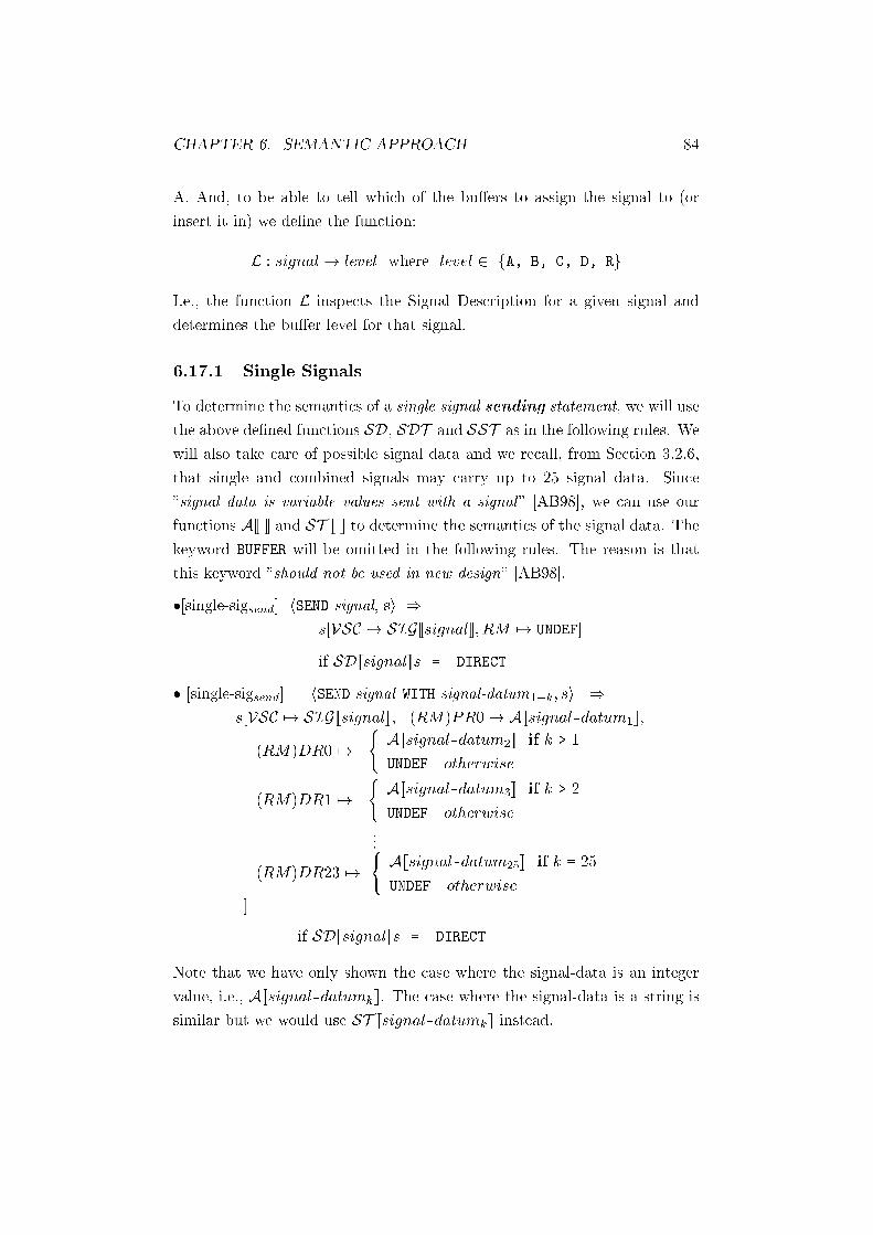
CHAPTER 6. SEMANTIC APPROACH 84
A. And, to be able to tell which of the bu�ers to assign the signal to (or
insert it in) we de�ne the function:
L : signal! level where level 2 fA, B, C, D, Rg
I.e., the function L inspects the Signal Description for a given signal and
determines the bu�er level for that signal.
6.17.1 Single Signals
To determine the semantics of a single signal sending statement, we will use
the above de�ned functions SD, SDT and SST as in the following rules. We
will also take care of possible signal data and we recall, from Section 3.2.6,
that single and combined signals may carry up to 25 signal data. Since
�signal data is variable values sent with a signal� [AB98], we can use our
functions A[[ ]] and ST [[ ]] to determine the semantics of the signal data. The
keyword BUFFER will be omitted in the following rules. The reason is that
this keyword �should not be used in new design� [AB98].
�[single-sigsend] hSEND signal, si )
s[VSC 7! SIG[[signal]]; RM 7! UNDEF]
if SD[[signal]]s = DIRECT
� [single-sigsend] hSEND signal WITH signal-datum1�k; si )
s[VSC 7! SIG[[signal]]; (RM)PR0 7! A[[signal-datum1]];
(RM)DR0 7!
(A[[signal-datum2]] if k > 1
UNDEF otherwise
(RM)DR1 7!
(A[[signal-datum3]] if k > 2
UNDEF otherwise...
(RM)DR23 7!
(A[[signal-datum25]] if k = 25
UNDEF otherwise
]
if SD[[signal]]s = DIRECT
Note that we have only shown the case where the signal-data is an integer
value, i.e., A[[signal-datumk]]. The case where the signal-data is a string is
similar but we would use ST [[signal-datumk]] instead.
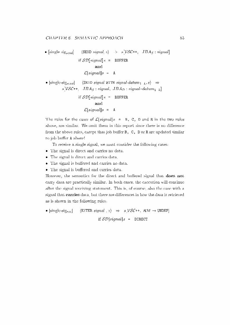
CHAPTER 6. SEMANTIC APPROACH 85
� [single-sigsend] hSEND signal, si ) s[VSC++; JBAS : signal]
if SD[[signal]]s = BUFFER
and
L[[signal]]s = A
� [single-sigsend] hSEND signal WITH signal-datum1�k; si )
s[VSC++; JBAS : signal; JBAD : signal-datum1�k]
if SD[[signal]]s = BUFFER
and
L[[signal]]s = A
The rules for the cases of L[[signal]]s = B, C, D and R in the two rules
above, are similar. We omit them in this report since there is no di�erence
from the above rules, except that job bu�er B, C, D or R are updated similar
to job bu�er A above!
To receive a single signal, we must consider the following cases:
� The signal is direct and carries no data.
� The signal is direct and carries data.
� The signal is bu�ered and carries no data.
� The signal is bu�ered and carries data.
However, the semantics for the direct and bu�ered signal that does not
carry data are practically similar. In both cases, the execution will continue
after the signal receiving statement. This is, of course, also the case with a
signal that carries data, but there are di�erences in how the data is retrieved
as is shown in the following rules.
� [single-sigrec] hENTER signal , si ) s[VSC++; RM 7! UNDEF]
if SD[[signal]]s = DIRECT

CHAPTER 6. SEMANTIC APPROACH 86
� [single-sigrec] hENTER signal WITH signal-datum1�k, si )
s[VSC++; (RM)PR0 7! A[[signal-datum1]];
(RM)DR0 7!
(A[[signal-datum2]] if k > 1
UNDEF otherwise
(RM)DR1 7!
(A[[signal-datum3]] if k > 2
UNDEF otherwise...
(RM)DR23 7!
(A[[signal-datum25]] if k = 25
UNDEF otherwise
]
if SD[[signal]]s = DIRECT
Actually, the signal data has already been put in the register memory (RM)
by the APZ Operating System, which, of course, is the case for all kinds of
transferring of signal data. We write the rule in this way just to make it
explicit where the signal data is located.
In a similar way to when we inserted a signal (and its data) to a job
bu�er, and used the notation JBAS:sig and JBAD:sig-data, we will write
sig:JBAS and signal-datum1-k:JBAD to denote the contents of the job
bu�er (A in this case) before the statement is executed whereas the contents
of the job bu�er, after we have fetched a signal and its eventual data, is
denoted JBAD and JBAS which indicates that the �rst item in the bu�er
has been removed.
With the same argumentation as with the sending of a single/bu�ered
signal above, we omit the rules for receiving a single/bu�ered signal from
any of the bu�ers B - R since there is no di�erence except which bu�er is to
be updated.
� [single-sigrec] hENTER signal , s[signal : JBAS ]i )
s[VSC++; JBAS ; RM 7! UNDEF]
if SD[[signal]]s = BUFFER
and
L[[signal]]s = A

CHAPTER 6. SEMANTIC APPROACH 87
� [single-sigrec] hENTER signal WITH signal-datum1�k;
s[signal : JBAS ; signal-datum1-k : JBAD]i )
s[VSC++; JBAD; JBAS;
(RM)PR0 7! A[[signal-datum1]];
(RM)DR0 7!
(A[[signal-datum2]] if k > 1
UNDEF otherwise
(RM)DR1 7!
(A[[signal-datum3]] if k > 2
UNDEF otherwise...
(RM)DR23 7!
(A[[signal-datum25]] if k = 25
UNDEF otherwise
]
if SD[[signal]]s = BUFFER
and
L[[signal]]s = A
6.17.2 Combined Signals
As stated in the beginning of Section 6.17, the distinction that is of interest is
between direct and bu�ered signals. The syntactical distinction between sin-
gle and combined signals is of secondary interest since the combined signals
are semantically equal to the single signals, with one exception, namely
the sending of a combined forward signal. This is due to the fact that the
control of the execution will return to the �caller�37.
According to the above, all but one rule for the semantics of combined
signals are given in shortened versions together with a few comments. We
refer to Appendix A for the complete set of rules.
The sending of a combined forward signal is in many ways similar to the
sending of a (direct) single signal. However, there are two things that we
must take into consideration when we specify the following rule38.
1. We must be able to tell what happens on �the other side�. I.e., we must
37From a semantical point of view, the combined signals can be viewed as direct signals
since a combined signal can never be bu�ered 3.2.38We will omit the �REFERENCE �eld-variable� part (see Section 6.9.2) since this part
does not change the meaning of the statement.

CHAPTER 6. SEMANTIC APPROACH 88
be able to trace the execution in the receiving part.
2. We must also handle the �reply�, i.e, the jump back. (Recall from
Section 3.2.3 that the execution always returns to the �caller�.)
To be able to trace the execution in the receiving part, we will de�ne the
code to be executed as a CodeBlock and let blockn be a meta-variable ranging
over CodeBlock. blockn is de�ned as
� blockn ::= S; RET
� S ::= Statement; S | "
� Statement ::= Any of the PLEX statements described in Section 6.4
- 6.10 except for the following statements: RECEIVE, RETURN,
ENTER or EXIT.
� RET ::= IF expressionRETURN cbsig ELSE RET |RETURN cbsig
I.e., we de�ne CodeBlock as a sequence of PLEX statements with a Single-
Entry-Multiple-Exit �semantics�.
To �fetch� a codeblock, we will use the following function
BLOCK : address! CodeBlock
which takes an address (which will be the value of our statement counter
VSC) and returns the corresponding CodeBlock. Finally, to specify the
meaning of this CodeBlock, we will use the function SPLEX . The function
will not be de�ned before Section 6.19, but we can already say that this
function will determine the meaning of a sequence of PLEX statements.

CHAPTER 6. SEMANTIC APPROACH 89
� [combined-sig-fwdsend]
hRECEIVE cfsig; s[VSC 7! SIG[[cfsig]]s; RM 7! UNDEF]i ) s0;SPLEX [[block1]]s0 ) s00
hSEND cfsig WAIT FOR cbsig1 IN label1 OR ::: cbsign IN labeln; si) s00[VSC 7! label]
where label =
8>><>>:ADR[[label1]] if RM(PR0) = cbsig1
...
ADR[[labeln]] if RM(PR0) = cbsign
and
block1 = BLOCK[[VSC0++]]
NOTE: Recall that the last statement in block1 is a RETURN cbsigk and
that the name of the return signal is found in the �rst register (PR0) of the
Register Memory (RM).
The case where the combined forward signal carries signal data is equiv-
alent except that the register memory (RM) is updated with the data. We
omit this case since there is no other di�erence from the above rule!
� [combined-sig-fwdrec] hRECEIVE cfsignal [WITH signal-datum], si )
s[VSC++; : : :]
From the receiver's point of view, it is of no interest whether the signal it
receives is a single signal or a combined signal. The execution will continue
with the statement that follows the receiving statement, which is shown
above. Depending on if the signal does carry any data, the register memory
(RM) is updated in the same way as with a single signal. (See Appendix A.)
� [combined-sig-bwdsend ] hRETURN cbsignal [WITH signal-datum], si )
s[VSC 7! SIG[[cbsignal]]; : : :]
Sending a combined backward signal, means an immediate reply to the ini-
tiating block/sender, i.e. a direct signal. Again, we refer to Appendix A for
a description on how the register memory is updated (which is similar to the
updating in case of a single, direct signal).
� [combined-sig-bwdrec ]
hlabel ')' RETRIEVE cbsignal [WITH signal-datum], si )
s[VSC++; : : :]

CHAPTER 6. SEMANTIC APPROACH 90
The same argumentation as with the combined forward receiving statement
above. After the receiving of the signal the execution continues with the
statement that follows the receiving statement. Appendix A shows how the
register memory is updated (in case of signal data).
6.17.3 The Semantics for Local Signals
Since the local signals are similar to direct signals (Section 3.2.4), their se-
mantics could be regarded as similar to the semantics for the single-direct
signals (Section 6.17.1). But, since they are implemented as a direct jump,
their semantics could also be seen as similar to the semantics for uncondi-
tional jumps (Section 6.13). It is also said that �a simple GOTO statement
could replace a local signal � [AB98]. From the same source, we also �nd out
that local signals is not transferred via the Signal Distribution Table, which
means that we can not use the same functions as in Section 6.17.1.
To solve our �problem�, we will make use of the following fact: Since the
signal is local, the receiving point is found in the same SPI (Section 2.2.1).
This means that we can use the signal name as a label and �combine� the
semantics for the unconditional jump and the single-direct signals! As for
the previous signal statements, we will separate the case when no data is
sent with the signal from the case when the signal carry one or more (up to
25) signal data.
The main di�erence between local and �global�39 signals are that local
signals preserve the temporary variables, i.e., the contents of the register
memory (RM) is left unchanged if no signal data is transferred along with
the signal. This will be shown in the following rules.
� [local-sigsend] hTRANSFER signal-name, si )
s[VSC 7! ADR[[signal-name]] ]
39By �global� signals we mean signals that are not local.

CHAPTER 6. SEMANTIC APPROACH 91
�[local-sigsend] hTRANSFER signal-name WITH signal-datum1�k; si )
s[VSC 7! ADR[[signal-name]]; (RM)PR0 7! signal-datum1;
(RM)DR0 7!
(A[[signal-datum2]] if k > 1
(RM)DR0 otherwise...
(RM)DR23 7!
(A[[signal-datum25]] if k = 25
(RM)DR23 otherwise
]
� [local-sigrec] hENTRANCE signal-name, si ) s[VSC++]
�[local-sigrec] hENTRANCE signal-name WITH signal-datum1�k; si )
s[VSC++; (RM)PR0 7! signal-datum1;
(RM)DR0 7!
(A[[signal-datum2]] if k > 1
(RM)DR0 otherwise...
(RM)DR23 7!
(A[[signal-datum25]] if k = 25
(RM)DR23 otherwise
]
6.18 The Semantics for the EXIT-statement
As explained in Section 6.10, the EXIT statement is a deactivation statement
for a sequence of statements. The meaning of the EXIT statement is that
the control is transferred back to the operating system (APZ), which selects
the next signal to execute based on the contents of the job bu�ers. This
means, in a sense, that we move our semantic approach away from the level
of statements and look at what's going on in the operating system. I.e., the
semantics of the EXIT statement is more a question of the semantics for the
execution model than the language40. However, in contradiction to the job
bu�er pointers, the EXIT statement is part of the language, and is therefore
treated here. To be able to capture what happens after an EXIT statement,
we introduce the partial function
APZ : state ,! state
40See also Section 6.17 where the similar argumentation is made on the job bu�er
pointers.

CHAPTER 6. SEMANTIC APPROACH 92
which inspects the current state and assign the �rst �ready-job� to our state-
ment counter, VSC. It is de�ned in Table 6.5.
The function is partial function since it is unde�ned in the case of all job
bu�ers being empty at the same time. The absence of a transition in this
situation models the fact that the system �goes idle�, i.e., it will simply wait
for a RP-CP signal (see Section 3.2 and Fig. 3.2) to arrive in any of the job
bu�ers.
So, with the introduction of APZ we can specify the semantics of the
EXIT statement as
� [exit] hEXIT, si ) s[VSC 7! APZ(s); RM 7! UNDEF]
APZ(s) =
8>>>>>>>>>>>>>>>>>>>>>>>>>>>>>>>>>>>><>>>>>>>>>>>>>>>>>>>>>>>>>>>>>>>>>>>>:
s[VSC 7! first(JBA)] if s[JBA] 6= ;41
s[VSC 7! first(JBB)] if s[JBA] = ; and
if s[JBB] 6= ;
s[VSC 7! first(JBC)] if s[JBA] = ; and
if s[JBB] = ; and
if s[JBC] 6= ;
s[VSC 7! first(JBD)] if s[JBA] = ; and
if s[JBB] = ; and
if s[JBC] = ; and
if s[JBD] 6= ;
undef if s[JBA] = ; and
if s[JBB] = ; and
if s[JBC] = ; and
if s[JBD] = ;
Table 6.5: The function APZ which fetches the �rst �ready-job� with highest
priority.
41JBA = ; is the same as JBI = JBO, i.e., Job Bu�er In = Job Bu�er Out. (See Section
6.2.)

CHAPTER 6. SEMANTIC APPROACH 93
6.19 The Semantic Function SPLEX
In the previous sections (6.12 - 6.18) we have speci�ed how the execution of
single PLEX statements change the state of the system. In this section we
will de�ne the meaning of a sequence of statements. But as claimed in Sec-
tion 1.2, the semantics for sequences of statements is restricted to well-formed
constructs (i.e., well-formed sequences of statements). These sequences have
a single-entry-multiple-exit semantics. They are entered through an EN-
TER or a RECEIVE statement and left with an EXIT or a RETURN
statement. The entering of such a sequence, via one of the above statements,
must be through a signal sending statement. I.e., every entering statement
must be preceded by an exit statement (EXIT or RETURN) which un-
conditionally breaks the �normal� sequential execution order. And, since we
say that these constructs have a single-entry semantics, we do not alove a
second entering statement before an exit statement!
To specify the semantics for sequences of statements in a proper way,
there are two important things that we must take into consideration:
1. We must capture the possibility of a �non-sequencial� execution order.
I.e., the possible occurrence of a GOTO statement must be handled.
2. An EXIT statement aborts the execution and none of the statements
that may follow in the source code �le will be executed.
To specify the meaning of a sequence of statements, we �rst denote the
syntactic category of sequences of statements, terminated by an EXIT state-
ment or an unconditional GOTO statement, as Code and let cn be a meta-
variable ranging over Code. cn is then de�ned as
� cn ::= S; OUT
� S ::= Statement; S | "
� Statement ::= Any of the PLEX statements described in Section 6.4
- 6.10 except for the EXIT statement (Section 6.18) and the uncon-
ditional jump, GOTO, (Section 6.5).
� OUT ::= EXIT | GOTO label
Then, we de�ne the function
CODE : address! code

CHAPTER 6. SEMANTIC APPROACH 94
to be the function that takes an address (which will be the value of our
statement counter, VSC) and returns the code sequence that starts at the
given address.
The meaning of a sequence of statements is now given by the function
SPLEX :
SPLEX [[S; c1]]s =
8>>>>>>>>>><>>>>>>>>>>:
s0 if hS; si ) s0 and c1 = "
s0 if hS; si ) s0 and S = EXIT
SPLEX [[c1]]s0 if hS; si ) s0 and VSC0 = VSC++
SPLEX [[c2]]s0 if hS; si ) s0; VSC0 6= VSC++;
and c2 = CODE [[VSC0]]
Note, the last case expresses the fact that the sequential execution order
is �broken� (for example by a GOTO statement) and the execution is �trans-
ferred� somewhere di�erent from the following statement.
So, with the de�nition of SPLEX we have �nally speci�ed the semantics
for individual PLEX statements as well as for sequences of statements. And
by this, we have also speci�ed the semantics of an entire job (Section 3.3.1)
since SPLEX determines the meaning of an arbitrary sequence of statements
which could very well start with an ENTER statement and end with an EXIT
statement (which constitutes a job).

Chapter 7
Summary
This report presents a structural operational semantics for the language
PLEX, a single-purpose and event-based real-time language developed by
Ericsson and used exclusively in telephony systems, i.e., in central parts of
the AXE switching system (from Ericsson). We have presented a formal
description of fundamental parts of the language, which is considered to be
jumps and signal sending statements.
By means of the semantics presented in this report, a formal basis for fur-
ther investigations and comparisons with other languages is provided since
the meaning, i.e. the semantics, of the language now is explicit. The seman-
tics presented could also be seen as a reference manual when the language is
implemented for new hardware platforms.
The language PLEX and its execution model are tightly connected and
it is not possible to separate one from another. For a complete semantic over
the language, one also have to consider the semantics of the execution model.
This report takes the �rst step towards a semantic de�nition of the execution
model of PLEX, and hence to a complete semantic de�nition of the language.
The report should also be seen in a further perspective, where the aim
is to extend and modify the language with a possibility to run in a multi-
processor environment, as described in Section 1.1. With a semantic descrip-
tion of the fundamental parts of the language, an important step towards
the multi-processor environment has been taken since the semantics of the
execution model is fundamental for this work, and as shown above, this work
takes a �rst step towards de�ning the execution model formally.
95

Bibliography
[AB86] Ericsson Telecom AB. PLEX Reference Manual, 1986.
[AB98] Ericsson Telecom AB. PLEX-C 1 Course book, 1998.
[AB02] Ericsson Telecom AB. PLEX-C Language Description, 2002.
[AE00] J. Axelsson and J. Erikson. SAPP, Theories and Tools for Ex-
ecution Time Estimation for Soft Real Time (Communication)
Systems. Master's thesis, Mälardalen University, 2000.
[AGG99] A. Arnstrom, C. Grosz, and A. Guillemot. GRETA: a tool con-
cept for validation and veri�cation of signal based systems (e.g.
written in PLEX). Master's thesis, Mälardalen University, 1999.
[BJ82] D. Bjørner and C. B. Jones. Formal Speci�cation and Software
Development. Prentice-Hall, 1982.
[EGG+01] R. Eschbach, U. Glässer, R. Gotzhein, M. von Löwis, and
A. Prinz. Formal De�nition of SDL-2000: Compiling and Run-
ning SDL Speci�cations as ASM Models. Journal of Universal
Computer Science, 11(7):1025�1050, 2001.
[EL02] J. Erikson and B. Lindell. The Execution Model of the
APZ/PLEX - An Informal Description. Technical report,
Mälardalen University, 2002.
[Her99] D. Herzberg. UML-RT as a Candidate for Modeling Embed-
ded Real-Time Systems in the Telecommunication Domain. In
Proceedings of the Second International Conference on UML
(UML'99),LNCS 1723, Springer, 1999.
[IT82] ITU-T. CHILL: Formal De�nition, 1982. International Telecom-
munication Union, Volume 1, Part 1, 2, 3.
96

BIBLIOGRAPHY 97
[IT99] ITU-T. CHILL: The ITU-T programming Language, 11 1999.
International Telecommunication Union, Geneva, (Recommen-
dation Z.200).
[IT00] ITU-T. SDL Formal Semantics De�nition, 2000. ITU-T Re-
comendation Z.100 Annex F.
[KP96] Al Kelley and Ira Pohl. C By Dissection - The Essentials of C
Programming. Addison-Wesley, 1996.
[Lin03] B. Lindell. Analysis of reentrancy and problems of data inter-
ference in the parallel execution of a multi processor AXE-APZ
system. Master's thesis, Mälardalen University, 2003.
[Lis98] B. Lisper. Semantical Tidbits, 1998.
[Mos01] P. D. Mosses. The Varieties of Programming Language Semantics
(and Their Uses). In Lecture Notes in Computer Science, Vol.
2244, pages 165 � 190, 2001.
[NN92] H. R. Nielson and F. Nielson. Semantics with Applications: A
Formal Introduction. John Wiley & Sons, 1992.
[Win00] Jürgen F. H. Winkler. CHILL 2000. Telektronikk, 96(4):70�77,
2000.
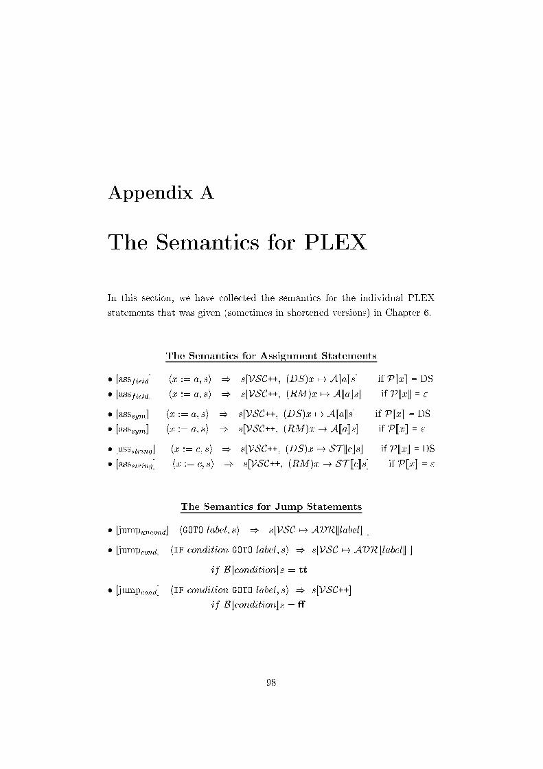
Appendix A
The Semantics for PLEX
In this section, we have collected the semantics for the individual PLEX
statements that was given (sometimes in shortened versions) in Chapter 6.
The Semantics for Assignment Statements
� [assfield] hx := a; si ) s[VSC++; (DS)x 7! A[[a]]s] if P[[x]] = DS
� [assfield] hx := a; si ) s[VSC++; (RM)x 7! A[[a]]s] if P[[x]] = "
� [asssym] hx := a; si ) s[VSC++; (DS)x 7! A[[a]]s] if P[[x]] = DS
� [asssym] hx := a; si ) s[VSC++; (RM)x 7! A[[a]]s] if P[[x]] = "
� [assstring] hx := c; si ) s[VSC++; (DS)x 7! ST [[c]]s] if P[[x]] = DS
� [assstring] hx := c; si ) s[VSC++; (RM)x 7! ST [[c]]s] if P[[x]] = "
The Semantics for Jump Statements
� [jumpuncond] hGOTO label; si ) s[VSC 7! ADR[[label]] ]
� [jumpcond] hIF condition GOTO label; si ) s[VSC 7! ADR[[label]] ]
if B[[condition]]s = tt
� [jumpcond] hIF condition GOTO label; si ) s[VSC++]
if B[[condition]]s = �
98

APPENDIX A. THE SEMANTICS FOR PLEX 99
The Semantics for Conditional Statements
� [condif ] hIF condition THEN S1; si ) hS1; si
if B[[condition]]s = tt
� [condif ] hIF condition THEN S1; si ) s[VSC++]
if B[[condition]]s = �
� [condif ] hIF condition THEN S1 ELSE S2; si ) hS1; si
if B[[condition]]s = tt
� [condif ] hIF condition THEN S1 ELSE S2; si ) hS2; si
if B[[condition]]s = �
The Semantics for Selection Statements
� [select] hCASE expression IS WHEN choice DO S1
OTHERWISE DO Sn; si ) hS1; si
if B[[expression = choice]]s = tt
� [select] hCASE expression IS WHEN choice DO S1
OTHERWISE DO Sn; si ) hSn; si
if B[[expression = choice]]s = �
The Semantics for Iteration Statements
� [ONUp]
hS; si ) s0; hON point=var FROM exp1+1 UPTO exp2 DO S; s0i) s00
hON point=var FROM exp1 UPTO exp2 DO S; si ) s00
if A[[exp1]]s < A[[exp2]]s
� [ONUp] hON pointer/variable FROM 'expression1' UPTO
'expression2' DO S; si ) s[VSC++]
if A[[expression1]]s > A[[expression2]]s
� [ONDown]
hS; si ) s0; hON point=var FROM exp1�1 DOWNTO exp2 DO S; s0i) s00
hON point=var FROM exp1 DOWNTO exp2 DO S; si ) s00
if A[[exp1]]s > A[[exp2]]s

APPENDIX A. THE SEMANTICS FOR PLEX 100
� [ONDown] hON pointer/variable FROM 'expression1' DOWNTO
'expression2' DO S; si ) s[VSC++]
if A[[expression1]]s < A[[expression2]]s
� [FORALL]
hS; si ) s0;
hFOR ALL pointer=field-var FROM field-exp1 - 1 DO S; s0i ) s00
hFOR ALL pointer=field-var FROM field-exp1 DO S; si ) s00
if A[[field� exp1]]s > 0
� [FORALL] hFOR ALL pointer/�eld-variable FROM �eld-expression1
DO S/statement-block-name, si ) s[VSC++]
if A[[field-expression1]]s < 0
� [FORFIRST ] hFOR FIRST pointer/�eld-variable FROM �eld-expression1
WHERE condition | �eld-variable IS CHANGED TO
�eld-expression GOTO label, si ) s[VSC 7! ADR[[label]] ]
if A[[field-expression1]]s >= 0
and
B[[condition|field-variable = field-expression]]s = tt
� [FORFIRST ] hFOR FIRST pointer/�eld-variable FROM �eld-expression1
WHERE condition | �eld-variable IS CHANGED TO
�eld-expression DO S/statement-block-name, si )
hS/statement-block-name-name, si
if A[[field-expression1]]s >= 0
and
if B[[condition|field-variable = field-expression]]s = tt
� [FORFIRST ] hFOR FIRST pointer/�eld-variable FROM �eld-expression1
WHERE condition | �eld-variable IS CHANGED TO
�eld-expression GOTO label, si )
hFOR FIRST pointer/�eld-variable FROM �eld-expression1-1
WHERE condition | �eld-variable IS CHANGED TO
�eld-expression GOTO label, si
if A[[field-expression1]]s >= 0
and
if B[[condition|field-variable = field-expression]]s = �

APPENDIX A. THE SEMANTICS FOR PLEX 101
� [FORFIRST ] hFOR FIRST pointer/�eld-variable FROM �eld-expression1
WHERE condition | �eld-variable IS CHANGED TO
�eld-expression DO S/statement-block-name, si )
hFOR FIRST pointer/�eld-variable FROM �eld-expression1-1
WHERE condition | �eld-variable IS CHANGED TO
�eld-expression DO S/statement-block-name, si
if A[[field-expression1]]s >= 0
and
if B[[condition|field-variable = field-expression]]s = �
� [FORFIRST ] hFOR FIRST pointer/�eld-variable FROM �eld-expression1
DO S/statement-block-name, si ) s[VSC++]
if A[[field-expression1]]s < 0
The Semantics for Signal Statements
�[single-sigsend] hSEND signal, si )
s[VSC 7! SIG[[signal]]; RM 7! UNDEF]
if SD[[signal]]s = DIRECT
�[single-sigsend] hSEND signal WITH signal-datum1�k; si )
s[VSC 7! SIG[[signal]]; (RM)PR0 7! A[[signal-datum1]];
(RM)DR0 7!
(A[[signal-datum2]] if k > 1
UNDEF otherwise
(RM)DR1 7!
(A[[signal-datum3]] if k > 2
UNDEF otherwise...
(RM)DR23 7!
(A[[signal-datum25]] if k = 25
UNDEF otherwise
]
if SD[[signal]]s = DIRECT
� [single-sigsend] hSEND signal, si ) s[VSC++; JBAS : signal]
if SD[[signal]]s = BUFFER
and
L[[signal]]s = A

APPENDIX A. THE SEMANTICS FOR PLEX 102
� [single-sigsend] hSEND signal WITH signal-datum1�k; si )
s[VSC++; JBAS : signal; JBAD : signal-datum1�k]
if SD[[signal]]s = BUFFER
and
L[[signal]]s = A
�[single-sigrec] hENTER signal , si ) s[VSC++; RM 7! UNDEF]
if SD[[signal]]s = DIRECT
�[single-sigrec] hENTER signal WITH signal-datum1�k; si )
s[VSC++; (RM)PR0 7! A[[signal-datum1]];
(RM)DR0 7!
(A[[signal-datum2]] if k > 1
UNDEF otherwise
(RM)DR1 7!
(A[[signal-datum3]] if k > 2
UNDEF otherwise...
(RM)DR23 7!
(A[[signal-datum25]] if k = 25
UNDEF otherwise
]
if SD[[signal]]s = DIRECT
� [single-sigrec] hENTER signal , s[signal : JBAS ]i )
s[VSC++; JBAS ; RM 7! UNDEF]
if SD[[signal]]s = BUFFER
and
L[[signal]]s = A

APPENDIX A. THE SEMANTICS FOR PLEX 103
� [single-sigrec] hENTER signal WITH signal-datum1�k;
s[signal : JBAS ; signal-datum1-k : JBAD]i )
s[VSC++; JBAD; JBAS;
(RM)PR0 7! A[[signal-datum1]];
(RM)DR0 7!
(A[[signal-datum2]] if k > 1
UNDEF otherwise
(RM)DR1 7!
(A[[signal-datum3]] if k > 2
UNDEF otherwise...
(RM)DR23 7!
(A[[signal-datum25]] if k = 25
UNDEF otherwise
]
if SD[[signal]]s = BUFFER
and
L[[signal]]s = A
� [combined-sig-fwdsend]
hRECEIVE cfsig; s[VSC 7! SIG[[cfsig]]s; RM 7! UNDEF]i ) s0;SPLEX [[block1]]s0 ) s00
hSEND cfsig WAIT FOR cbsig1 IN label1 OR ::: cbsign IN labeln; si) s00[VSC 7! label]
where label =
8>><>>:ADR[[label1]] if RM(PR0) = cbsig1
...
ADR[[labeln]] if RM(PR0) = cbsign
and
block1 = BLOCK[[VSC0++]]
� [combined-sig-fwdrec] hRECEIVE cfsignal, si )
s[VSC++; RM 7! UNDEF]

APPENDIX A. THE SEMANTICS FOR PLEX 104
� [combined-sig-fwdrec] hRECEIVE cfsignal WITH signal-datum1�k; si )
s[VSC++; (RM)PR0 7! A[[signal-datum1]];
(RM)DR0 7!
(A[[signal-datum2]] if k > 1
UNDEF otherwise
(RM)DR1 7!
(A[[signal-datum3]] if k > 2
UNDEF otherwise...
(RM)DR23 7!
(A[[signal-datum25]] if k = 25
UNDEF otherwise
]
� [combined-sig-bwdsend ] hRETURNcbsignal; si )
s[VSC 7! SIG[[cbsignal]]; RM 7! UNDEF]
� [combined-sig-bwdsend] hRETURN cbsignal WITH signal-datum1�k; si )
s[VSC 7! SIG[[cbsignal]]; (RM)PR0 7! A[[signal-datum1]];
(RM)DR0 7!
(A[[signal-datum2]] if k > 1
UNDEF otherwise
(RM)DR1 7!
(A[[signal-datum3]] if k > 2
UNDEF otherwise...
(RM)DR23 7!
(A[[signal-datum25]] if k = 25
UNDEF otherwise
]
� [combined-sig-bwdrec ]
hlabel0)0 RETRIEVE cbsignal; si ) s[VSC++; RM 7! UNDEF]
� [combined-sig-bwdrec ]
hlabel0)0 RETRIEVEcbsignal[WITH signal � datum]; si )
s[VSC++; (RM)PR0 7! A[[signal-datum1]];
(RM)DR0 7!
(A[[signal-datum2]] if k > 1
UNDEF otherwise
(RM)DR1 7!
(A[[signal-datum3]] if k > 2
UNDEF otherwise...
(RM)DR23 7!
(A[[signal-datum25]] if k = 25
UNDEF otherwise
]

APPENDIX A. THE SEMANTICS FOR PLEX 105
� [local-sigsend] hTRANSFER signal-name; si )
s[VSC 7! ADR[[signal-name]] ]
�[local-sigsend] hTRANSFER signal-name WITH signal-datum1�k; si )
s[VSC 7! ADR[[signal-name]]; (RM)PR0 7! signal-datum1;
(RM)DR0 7!
(A[[signal-datum2]] if k > 1
(RM)DR0 otherwise...
(RM)DR23 7!
(A[[signal-datum25]] if k = 25
(RM)DR23 otherwise
]
� [local-sigrec] hENTRANCE signal-name; si ) s[VSC++]
� [local-sigrec] hENTRANCE signal-name WITH signal-datum1�k; si )
s[VSC++; (RM)PR0 7! signal-datum1;
(RM)DR0 7!
(A[[signal-datum2]] if k > 1
(RM)DR0 otherwise...
(RM)DR23 7!
(A[[signal-datum25]] if k = 25
(RM)DR23 otherwise
]
The Semantics for the EXIT Statement
� [exit] hEXIT; si ) s[VSC 7! APZ(s); RM 7! UNDEF]

Appendix B
The Signal Description
There are two main documents for signals: The Signal Survey, which is a
listing of all the signals sent and received in a unit, and the Signal Descrip-
tion, which will be studied in this section. These documents are compiled
together with the Source Program Information1, SPI.
The Signal Description, SD, is the document that de�nes a signal. The
type of the signal, as well as the priority level of the signal is speci�ed in
this document. There is one SD for every signal and all SD's are stored in
special libraries. We will study how the SD �interact� with the SPI during
the code generation phase. But as a �rst attempt to capture the contents of
the SD, it could be seen as similar to the h-file in C that externally de�nes
a function (among other things).
The SD includes the following items:
� Name of the signal - Every signal has a name that, perhaps, captures
its functionality.
� Signal number - For internal documentation.
� Function - Used to make comments about functionality.
� Signal type - The signal type indicates whether the signal is Single
or Combined. There are three possible type speci�cations:
� Type 1: Single signal
1The Source Program Information is the �source code �le�, i.e., the document that we
normally call a program. See Section 2.2.1 for further details.
106

APPENDIX B. THE SIGNAL DESCRIPTION 107
� Type 2: Combined forward
� Type 3: Combined backward
If the signal isMultiple, this is indicated by adding the keywordMUL-
TIPLE to the signal type, like in: TYPE IS 1 MULTIPLE
A Unique signal has no indication at this point! (A signal is unique
�by default� if nothing else is stated.) If the signal is local, the keyword
LOCAL is added to the signal type.
� Possible return signal - For internal documentation.
� Possible sending block - For internal documentation.
� Possible receiving block - For internal documentation.
� Bu�er level - The priority level! In Section 3.3, it is described how
every signal is assigned a priority level, and how signals are stored in
di�erent job bu�ers (in case of a bu�ered signal). The bu�er level
states the priority level of the corresponding job and also in which job
bu�er the signal will be bu�ered (if it is to be bu�ered, i.e.).
NOTE: The bu�er level can have the following combinations:
� NO BUFFER: The signal is direct. (A combined signal is al-
ways direct, see Section 3.2.3.)
� LEVEL A/B/C/D BUFFER: The signal is bu�ered and uses
the job bu�er speci�ed. This combination overrides a possible use
of the HURRY option in the signal sending statement (see below).
� LEVEL A/B/C/D: The signal is bu�ered and uses the job
bu�er speci�ed, unless the keyword HURRY is used in the signal
sending statement, which indicates that the signal is direct.
� Signal data - Speci�cation of the �arguments� (i.e., the data) that the
signal is carrying.
� ID sector - For internal documentation.