structural algorithms for diagnostic system design · pdf filestructural algorithms for...
TRANSCRIPT

Structural Algorithms for Diagnostic
System Design Using Simulink Models
Master’s thesis
performed in Vehicular Systems
byLars Eriksson
Reg nr: LiTH-ISY-EX-3601-2004
10th January 2005

Structural Algorithms for Diagnostic
System Design Using Simulink Models
Master’s thesis
performed in Vehicular Systems,Dept. of Electrical Engineering
at Linkopings universitet
by Lars Eriksson
Reg nr: LiTH-ISY-EX-3601-2004
Supervisor: Mattias Krysander
Linkopings UniversitetMattias Nyberg
Scania CV AB
Examiner: Assistant Professor Erik Frisk
Linkopings Universitet
Linkoping, 10th January 2005


Avdelning, Institution
Division, DepartmentDatum
Date
Sprak
Language
Svenska/Swedish
Engelska/English
Rapporttyp
Report category
Licentiatavhandling
Examensarbete
C-uppsats
D-uppsats
Ovrig rapport
URL for elektronisk version
ISBN
ISRN
Serietitel och serienummer
Title of series, numberingISSN
Titel
Title
Forfattare
Author
Sammanfattning
Abstract
Nyckelord
Keywords
Today’s society depends on complex and technically advanced mechanical systems,often containing a variety of different components. Despite careful development andconstruction, some of these components may eventually fail. To avoid unnecessarydamage, for example environmental or financial, there is a need to locate anddiagnose these faults as fast as possible. This can be done with a diagnostic system,which should produce an alarm if there is a fault in the mechanical system and, ifpossible, indicate the reason behind it.
In model based diagnosis, a mathematical model of a fault free system is usedto detect if the monitored system contain any faults. This is done by constructingfault indicators, called fault tests, consisting of equations from different parts of themodel. Finding these parts is a time-consuming and demanding task, hence it ispreferable if as much as possible of this process can be automated. In this thesis analgorithm that finds all parts of a system that can be used to create these fault testsis presented. To make this analysis feasible, in industrial applications, a simplifiedversion of a system model called a structural model is used. Since the modelsconsidered in this thesis are implemented in the mathematical software Simulink, amethod for transforming Simulink models into analytical equations and structuralmodels is described. As a way of increasing the diagnostic performance for a modelbased diagnostic system, information about different faults, called fault models, canbe included in the model. However, since the models in this thesis are implementedin Simulink, there is no direct way in which this can be preformed. This thesisdescribes a solution to this problem. The correctness of the algorithms in this thesisare proved and they have been applied, with supreme results, to a Scania truckengine model.
Vehicular Systems,Dept. of Electrical Engineering581 83 Linkoping
10th January 2005
—
LITH-ISY-EX-3601-2004
—
http://www.vehicular.isy.liu.sehttp://www.ep.liu.se/exjobb/isy/2004/3601/
Structural Algorithms for Diagnostic System Design Using SimulinkModels
Strukturella Algoritmer for Design av Diagnossystem med Simulink-modeller
Lars Eriksson
××
Model based diagnosis, Structural methods, Diagnostic systems, Graphtheory, Decomposition

Abstract
Today’s society depends on complex and technically advanced mechani-cal systems, often containing a variety of different components. Despitecareful development and construction, some of these components mayeventually fail. To avoid unnecessary damage, for example environ-mental or financial, there is a need to locate and diagnose these faultsas fast as possible. This can be done with a diagnostic system, whichshould produce an alarm if there is a fault in the mechanical systemand, if possible, indicate the reason behind it.
In model based diagnosis, a mathematical model of a fault free sys-tem is used to detect if the monitored system contain any faults. Thisis done by constructing fault indicators, called fault tests, consistingof equations from different parts of the model. Finding these partsis a time-consuming and demanding task, hence it is preferable if asmuch as possible of this process can be automated. In this thesis analgorithm that finds all parts of a system that can be used to createthese fault tests is presented. To make this analysis feasible, in in-dustrial applications, a simplified version of a system model called astructural model is used. Since the models considered in this thesisare implemented in the mathematical software Simulink, a method fortransforming Simulink models into analytical equations and structuralmodels is described. As a way of increasing the diagnostic performancefor a model based diagnostic system, information about different faults,called fault models, can be included in the model. However, since themodels in this thesis are implemented in Simulink, there is no directway in which this can be preformed. This thesis describes a solutionto this problem. The correctness of the algorithms in this thesis areproved and they have been applied, with supreme results, to a Scaniatruck engine model.
Keywords: Model based diagnosis, Structural methods, Diagnosticsystems, Graph theory, Decomposition
v

vi

Acknowledgments
This work has been carried out at the department of Electrical En-gineering, division of Vehicular Systems at Linkopings University asa combined project between the department of Electrical Engineeringand Scania CV AB in Sodertalje.
I would like to express my gratitude to an number of people:
My excellent supervisors Mattias Krysander and Mattias Nyberg formany interesting and inspiring discussions during the work. The staffat Vehicular Systems, special thanks to Erik Frisk for being my exam-iner and Jan Aslund for helping me with some mathematical issues.My fellow master thesis students Gustav Arrhenius, Henrik Einars-son, Kristian Krigsman and John Nilsson at Scania, Sodertalje. MikaelRautio, Jonas Eriksson and especially Jonas Elmqvist for giving mevaluable feedback on my report. Thank you all!
Finally I would like to thank my beloved girlfriend Tina for coping withme during this work, and my mother and father for always believing inand supporting me throughout my education.
Linkoping, December 2004
Lars Eriksson
vii

viii
Contents
Abstract v
Acknowledgments vii
Notation xi
1 Introduction 1
1.1 Background . . . . . . . . . . . . . . . . . . . . . . . . . 1
1.2 Related Work . . . . . . . . . . . . . . . . . . . . . . . . 2
1.3 Problem Formulation . . . . . . . . . . . . . . . . . . . . 2
1.4 Objectives . . . . . . . . . . . . . . . . . . . . . . . . . . 3
1.5 Target Group . . . . . . . . . . . . . . . . . . . . . . . . 3
1.6 Thesis Outline . . . . . . . . . . . . . . . . . . . . . . . 3
1.7 Contributions . . . . . . . . . . . . . . . . . . . . . . . . 4
2 Diagnostic Theory 5
2.1 Terminology and Definitions . . . . . . . . . . . . . . . . 5
2.2 Diagnostic Systems . . . . . . . . . . . . . . . . . . . . . 6
2.3 Behavioral Modes . . . . . . . . . . . . . . . . . . . . . . 8
2.4 Structural Models and their Properties . . . . . . . . . . 11
2.4.1 Structural Models . . . . . . . . . . . . . . . . . 11
2.4.2 Bipartite Graphs . . . . . . . . . . . . . . . . . . 13
2.4.3 Structural Properties . . . . . . . . . . . . . . . . 13
3 Algorithms for Simulink 19
3.1 Transforming Simulink Models to Analytical Equations 19
3.1.1 Simulink Simplification . . . . . . . . . . . . . . 20
3.1.2 Deriving Analytical Equations from Simulink . . 21
3.1.3 Analytical Simplification . . . . . . . . . . . . . . 24
3.2 Structural Transformation . . . . . . . . . . . . . . . . . 25
3.3 Behavioral Modes in Simulink . . . . . . . . . . . . . . . 25
3.4 Fault Modeling in Simulink . . . . . . . . . . . . . . . . 26
ix
4 Structural Algorithms 29
4.1 Steps Toward Finding All MSO Sets . . . . . . . . . . . 294.2 Structural Simplification . . . . . . . . . . . . . . . . . . 304.3 Finding All MSO Sets . . . . . . . . . . . . . . . . . . . 33
4.3.1 Basic Algorithm . . . . . . . . . . . . . . . . . . 344.3.2 Improvements . . . . . . . . . . . . . . . . . . . . 36
4.4 Finding All MSO Sets in a Behavioral Mode System . . 394.5 The Correctness of the Algorithms . . . . . . . . . . . . 41
5 An Engine Model Example 47
5.1 Algorithm Efficiency . . . . . . . . . . . . . . . . . . . . 475.2 MSO Validation . . . . . . . . . . . . . . . . . . . . . . . 48
6 Conclusions and Future Work 52
6.1 Conclusions . . . . . . . . . . . . . . . . . . . . . . . . . 526.2 Future Work . . . . . . . . . . . . . . . . . . . . . . . . 53
References 55
x

Notation
Operators
|S| number of items in the set SM model i.e. a set of equationsX set of unknown variablesvarX′M set of variables in X ′ that are included in the model MequMX ′ set of equations in M that include some variable in X ′
G(M, varX′M) bipartite graph with vertex set M and X ′
var(G) set of all variable vertices in the graph Gequ(G) set of all equation vertices in the graph Gvar(γ) set of all variable vertices connected to an edge in
the edge set γequ(γ) set of all equation vertices connected to an edge in
the edge set γ
Abbreviations
SO Structurally OverdeterminedMSO Minimal Structurally OverdeterminedDSSM Differentiated-Separated Structural-ModelDLSM Differentiated-Lumped Structural-Model
xi

xii

Chapter 1
Introduction
This master’s thesis was performed at the department of ElectricalEngineering, division of Vehicular Systems at Linkopings University asa combined project between the department of Electrical Engineeringand Scania CV AB in Sodertalje. Scania is a worldwide manufacturer ofheavy duty trucks, buses and engines for marine and industrial use. Thework was carried out for the engine software development department,which is responsible for the engine control and the on board diagnostics(OBD) software.
1.1 Background
Today’s society depends on complex and technically advanced mechan-ical systems. Despite rigorous and careful development and construc-tion, some of the components in these systems may eventually fail. Toavoid unnecessary damage there is a need to locate and diagnose thesefailures as fast as possible. This can be illustrated through numerousexamples. Airplanes contain lots of safety critical systems. If a partof an engine begin to malfunction, it is important to detect this assoon as possible in order to carry out necessary maintenance. In theprocess industry a lot of money can be saved if a faulty componentcan be detected and replaced on a scheduled break in the manufactur-ing process, without causing any unplanned stop. The construction ofdiagnosis systems is therefore an important and necessary step in thedevelopment process for a lot of industrial applications.
Diagnosis of systems has been around for as long as there have beenmachines. In the beginning the diagnosis consisted in manual inspec-tions. With the introduction of computers, new ways of checking thecorrectness of systems was developed. Initially, techniques for detecting
1

2 Introduction
failures by analyzing signal levels of sensors were used. When a signallevel exceeded a predefined level at a specific working point the conclu-sion was that a failure had occurred. In addition to that, model baseddiagnosis was introduced. Model based diagnostic systems uses the un-derlying mathematical models for the physical components to diagnosethe components. This made it possible to base the entire diagnosticsystem on calculations. Using these model based diagnosis systems hasmade it possible to construct even more accurate and automated kindsof failure checking.
1.2 Related Work
This work can be seen as a link in a chain in the developing of modelbased diagnosis for engine systems. The objective is to develop methodsso that the whole procedure is as automated as possible. The workingprocess can schematically be described by the following list.
1. Construction of an engine model in Simulink.
2. Extracting model equations from the Simulink model.
3. Finding parts of the equation system that can be used for diag-nosis.
4. Constructing executable diagnostic tests for these parts.
The modeling work described in step (1) has been carried out in avariety of different phases and by different persons. For modeling workrelated the specific Scania truck engine mentioned in this thesis see [3].In this thesis, the emphasis is on step (2) and (3) in the list above.Work related to this has prior been presented by Mattias Krysanderin [7]. Parallel to this work, methods for handling step (4) has beendeveloped at Scania CV AB in Sodertalje. For a description of thiswork see [5].
1.3 Problem Formulation
Previous on-board diagnostic systems at Scania have mainly been man-ually constructed. These have been obtained through hard testing andsometimes an intuitive feeling of what part of an engine that can beused in the construction of a diagnostic system. This approach is bothtime consuming and ineffective. If for example a last minute changeis made in the engine, a total reconstruction of the diagnosis systemmay be necessary. Since the modeling work at Scania has been success-ful, creating models that are more and more accurate with low mean

1.4. Objectives 3
errors, model based diagnosis is becoming a realistic alternative to ex-isting methods. Model based diagnosis uses a mathematical descriptionof the system to be diagnosed i.e. the system can be described by aset of equations. This makes it possible to use automated tools inthe construction process of the diagnosis system. By using parts of theequation system, sensitive to specific faults, it is possible construct faultindicators, so-called fault tests. One problem is to find which parts ofthe equation system that can be used to construct these tests. Previousattempts to develop methods to find these parts have resulted in highlyineffective and computably demanding algorithms. This has made itimpossible to develop model based diagnosis, in the form described bythis work, for large and highly redundant models. Even though the partof the construction process described in this thesis do not have any realtime computation demand, it is desirable that the algorithms produceresults in matter of hours. Previous algorithms have had difficulties toproduce any results at all for the type of engine models considered inthis thesis, even if they have been running for days.
1.4 Objectives
The main objective of this thesis is to find all parts of an engine modelthat can be used in order to construct a diagnostic system i.e. tofind subsets of equations in the system model that can be used toindicate if something has failed. The existing algorithms for doing thisare inadequate since they, due to computational inefficiency, fails topresent results for certain kind of systems. Hence, there is an obviousneed to develop new versions of these algorithms. Since the modelis implemented in Matlab/Simulink there is also a need to find waysof transforming a Simulink model into analytical equations. In orderto increase the performance of the diagnostic system the concept ofbehavioral modes in Simulink will also be investigated.
1.5 Target Group
The target group of this work is primarily M.Sc./B.Sc. students withbasic knowledge in modeling work and some experience in using themodeling and simulation software Matlab/Simulink.
1.6 Thesis Outline
This section describes the outline of this thesis.
Chapter 2 gives an introduction to diagnostic theory. In order toincrease the ability for fault tests to pin point exactly what fault

4 Introduction
that have occurred in a system, so-called behavioral modes will beintroduced. The concept of structural models will be introducedas a solution to reduce the computing time for finding diagnosticfault tests.
Chapter 3 describes a solution to how a Simulink model may be trans-formed to model equations and how behavioral modes can beincluded into a Simulink model.
Chapter 4 presents new structural algorithms for extracting parts ofa system model that can be used to construct diagnostic tests. Inthe end of this chapter, these new algorithms are mathematicalverified by introducing a series of lemmas and theorems.
Chapter 5 present an industrial example with a Scania truck enginemodel. Compares and verifies the new algorithms by a series ofexecution tests.
Chapter 6 concludes this thesis by presenting the main results anddiscussing possible future work.
1.7 Contributions
In this section the main contributions of this thesis are listed.
• An algorithm that transforms Simulink models into analyticalequations.
• A method that describes how fault models can be included graph-ically into a Simulink model.
• An algorithm that simplifies a structural model.
• Algorithms for finding all parts of a system model that can beused when constructing a diagnostic system.
• New mathematical properties concerning structural models andgraph theory, for example the property of overdeterminedness.
• Mathematical verification of the derived algorithms through anumber of proved theorems and lemmas.
• The algorithms in this thesis provides a foundation toward a com-pletely automated construction process of model based diagnosticsystems.

Chapter 2
Diagnostic Theory
In this chapter some basic theory about diagnostic systems and theirproperties are presented. In the first section some commonly used def-initions regarding diagnosis will be explained. In the following sectionthe general concepts behind diagnosis systems and behavioral modesare discussed. Finally in the last section the theory behind structuralmethods is introduced. The theory in these sections is explained withemphasis on what is needed for understanding the following chapters.For a more thorough description on the subject see [4] and [2].
2.1 Terminology and Definitions
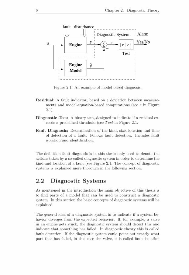
In Figure 2.1 an engine containing a diagnostic system is shown. Theengine behavior received from sensors y is compared to expected be-havior y calculated from an engine model. If these values diverge fromeach other more then a predefined threshold j, the diagnostic systemsignals that something is wrong.
In this section some of the terminology used in the field of diagnosis andin this thesis are explained. The following definitions are suggested bythe IFAC (International Federation of Automatic Control) TechnicalCommittee SAFEPROCESS and are given in [9].
Fault: An unpermitted deviation of at least one characteristic propertyor parameter of the system from the acceptable/usual/standardcondition.
Failure: A permanent interruption of a system’s ability to perform arequired function under specified operating conditions.
Disturbance: An unknown (and uncontrolled) input action on a sys-tem.
5
6 Chapter 2. Diagnostic Theory
Engine
EngineModel
∑ | r | > j
y
y
Alarm
u_
r Yes/No
Test
Diagnostic System
fault disturbance
Figure 2.1: An example of model based diagnosis.
Residual: A fault indicator, based on a deviation between measure-ments and model-equation-based computations (see r in Figure2.1).
Diagnostic Test: A binary test, designed to indicate if a residual ex-ceeds a predefined threshold (see Test in Figure 2.1.
Fault Diagnosis: Determination of the kind, size, location and timeof detection of a fault. Follows fault detection. Includes faultisolation and identification.
The definition fault diagnosis is in this thesis only used to denote theactions taken by a so-called diagnostic system in order to determine thekind and location of a fault (see Figure 2.1. The concept of diagnosticsystems is explained more thorough in the following section.
2.2 Diagnostic Systems
As mentioned in the introduction the main objective of this thesis isto find parts of a model that can be used to construct a diagnosticsystem. In this section the basic concepts of diagnostic systems will beexplained.
The general idea of a diagnostic system is to indicate if a system be-havior diverges from the expected behavior. If, for example, a valvein an engine gets stuck, the diagnostic system should detect this andindicate that something has failed. In diagnostic theory this is calledfault detection. If the diagnostic system could point out exactly whatpart that has failed, in this case the valve, it is called fault isolation

2.2. Diagnostic Systems 7
FaultsValve stuck Oil leak
Test 1 x xTest 2 x 0
Table 2.1: An example of a decision structure for a simple diagnosticsystem of an engine.
and is usually the aim of a diagnostic system.
In Figure 2.2 a schematic picture of the architecture in a diagnosticsystem is shown. Given observations, i.e. sensor values and actuatorvalues, the diagnostic system runs a number of diagnostic tests. Thetests are checking different parts of the system and returns binary val-ues indicating if the test detected a fault in the system or not, see Figure2.1. Since each of these tests usually is sensitive to a number of faults,isolation cannot directly be obtained. Therefore the results are sent toa fault isolation function. Using the combined results from the teststhe diagnostic system tries to isolate what specific part of the systemthat has failed and presents this as a diagnostic statement. In Table2.1 a simple example of fault isolation in a diagnostic system is shownwith a decision structure [4]. If a test in the diagnostic system becomesnon-zero the structure shows possible explanation. A x in the structureshows what faults a test may react to whereas the number 0 indicatethat the test is not sensitive to this specific fault. If for example Test 1in Table 2.1 becomes non-zero the only possible explanations are thatthere must be a stuck valve or an oil leak. If both tests signal that theyare indicating a fault, the fault isolation part of the diagnostic systemwill conclude that the valve is stuck.
In order for a diagnostic system to obtain fault indication there needsto be residuals able to indicate when a fault occur. In their simplestform these residuals are just a set of equations that equals zero if the su-pervised system is non-faulty. For example consider a system modeledas
x = uy = x
(2.1)
where u is an actuator signal, y is a sensor signal and x is an internalvariable. A residual that checks the correctness of this equation systemcan then be constructed as r1 = y − u. If the system behavior do notcoincide with the system model, the residual will not equal zero andthere is said to be a faulty system. As mentioned earlier the maingoal in most diagnostic systems is to isolate faults when they occur.
8 Chapter 2. Diagnostic Theory
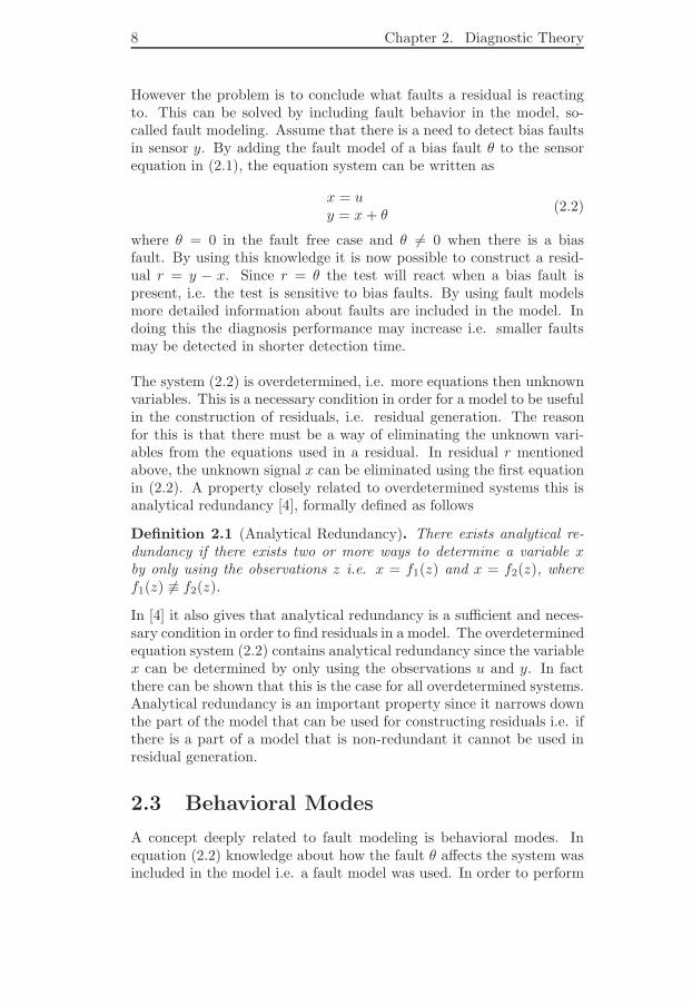
However the problem is to conclude what faults a residual is reactingto. This can be solved by including fault behavior in the model, so-called fault modeling. Assume that there is a need to detect bias faultsin sensor y. By adding the fault model of a bias fault θ to the sensorequation in (2.1), the equation system can be written as
x = uy = x + θ
(2.2)
where θ = 0 in the fault free case and θ 6= 0 when there is a biasfault. By using this knowledge it is now possible to construct a resid-ual r = y − x. Since r = θ the test will react when a bias fault ispresent, i.e. the test is sensitive to bias faults. By using fault modelsmore detailed information about faults are included in the model. Indoing this the diagnosis performance may increase i.e. smaller faultsmay be detected in shorter detection time.
The system (2.2) is overdetermined, i.e. more equations then unknownvariables. This is a necessary condition in order for a model to be usefulin the construction of residuals, i.e. residual generation. The reasonfor this is that there must be a way of eliminating the unknown vari-ables from the equations used in a residual. In residual r mentionedabove, the unknown signal x can be eliminated using the first equationin (2.2). A property closely related to overdetermined systems this isanalytical redundancy [4], formally defined as follows
Definition 2.1 (Analytical Redundancy). There exists analytical re-dundancy if there exists two or more ways to determine a variable xby only using the observations z i.e. x = f1(z) and x = f2(z), wheref1(z) 6≡ f2(z).
In [4] it also gives that analytical redundancy is a sufficient and neces-sary condition in order to find residuals in a model. The overdeterminedequation system (2.2) contains analytical redundancy since the variablex can be determined by only using the observations u and y. In factthere can be shown that this is the case for all overdetermined systems.Analytical redundancy is an important property since it narrows downthe part of the model that can be used for constructing residuals i.e. ifthere is a part of a model that is non-redundant it cannot be used inresidual generation.
2.3 Behavioral Modes
A concept deeply related to fault modeling is behavioral modes. Inequation (2.2) knowledge about how the fault θ affects the system wasincluded in the model i.e. a fault model was used. In order to perform

2.3. Behavioral Modes 9
Diagnostic
Diagnostic Test 1
Diagnostic Test n
.
.
.
FaultIsolation
Diagnostic Test 2Statement
Observations
Diagnostic System
Figure 2.2: The architecture of a diagnostic system.
systematic fault identification there is a need to classify and separatedifferent faults from each other. This can be done using so-called be-havioral modes. For example consider the model (2.2) again. Here twobehavioral modes can be defined, no fault (NF) and bias fault (B). Ifθ = 0 the system is in behavioral mode NF and if θ 6= 0 the systemis in behavioral mode B. Now assume that the system (2.2) has twosensors y1 and y2 both measuring the signal x. Also assume that thefirst sensor y1 can sustain a bias fault (B) while the other sensor y2 issensitive to a gain fault (G). The bias fault is in this case modeled bythe variable θ1 whereas the gain fault is model by θ2. The system canthen be written as
x = uy1 = x + θ1
y2 = θ2x(2.3)
By letting θ = [θ1 θ2] be a fault state vector the behavioral modes canbe defined as
Behavioral mode Fault StateNF θ = [0 1]B θ = [θ1 1; θ1 6= 0]G θ = [0 θ2; θ2 6= 1]
The reason for defining these modes is to be able to identify and isolatethe corresponding faults when they occur. For example consider theresiduals r1 = y1 − x and r2 = y2 − x of system (2.3). If residual r1 isnon-zero the system is said to be in behavioral mode B whereas resid-ual r2 is reacting then the system is said to be in behavioral mode G.If none of these tests react, then the system is in behavioral mode NF.
10 Chapter 2. Diagnostic Theory
Behavioral ModesNF B G UF
r1 0 x 0 xr2 0 0 x x
Table 2.2: Decision structure for system (2.3).
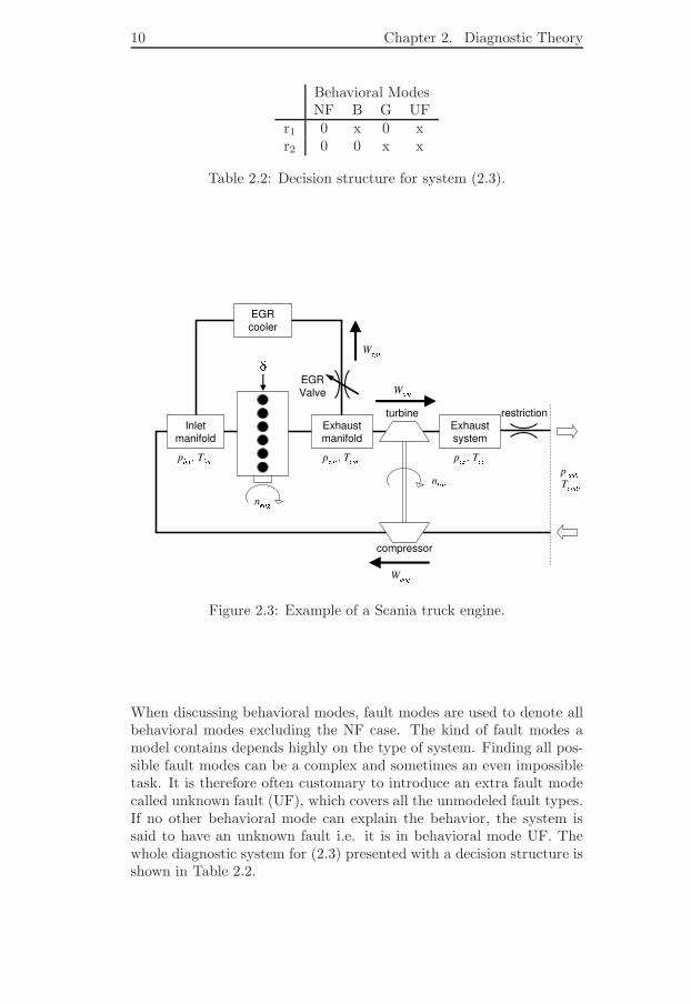
Figure 2.3: Example of a Scania truck engine.
When discussing behavioral modes, fault modes are used to denote allbehavioral modes excluding the NF case. The kind of fault modes amodel contains depends highly on the type of system. Finding all pos-sible fault modes can be a complex and sometimes an even impossibletask. It is therefore often customary to introduce an extra fault modecalled unknown fault (UF), which covers all the unmodeled fault types.If no other behavioral mode can explain the behavior, the system issaid to have an unknown fault i.e. it is in behavioral mode UF. Thewhole diagnostic system for (2.3) presented with a decision structure isshown in Table 2.2.

2.4. Structural Models and their Properties 11
2.4 Structural Models and their Proper-
ties
The diagnosis system is in this thesis applied to a Scania truck engineshown in Figure 2.3. The engine model is a large and complex system,containing eight actuator signals, four sensor signals and four states.The whole model is expressed using approximately 280 differential-algebraic equations. By Definition 2.1 there need to be analytical re-dundancy in order to construct a residual, i.e. there must be a way ofeliminating the unknown variables in the equation set used for a resid-ual. For example consider a system where u and y are known signalsand x3 = u and y = x. In order derive a residual based on these equa-tions the unknown variable x needs to be eliminated. This is done byfirst letting x = 3
√u and then constructing the residual as
r = y − 3√
u (2.4)
Hence all unknown variables can be eliminated and the two equationsx3 = u and y = x can be used to construct a valid residual.
While calculating the simple test in (2.4) one has to compute the cubic-root of a variable, a fairly demanding operation to perform. In theengine model it will not exist any tests of this simple form. In factexperiences have shown that the residuals in a Scania truck engine willinclude up to 300 equations. Due to combinatorial effects the numberof possible tests in the system will be in the range of 1000-10000. Toanalytically eliminate all the unknown variables in the search for validresiduals, like the one in (2.4), will be highly computational demanding,if even possible. In this thesis this problem is solved by using structuralmodels described in the following section.
2.4.1 Structural Models
The basic idea behind structural models is presented in [6]. Instead oflooking on the whole analytical expression of an equation, a less detailedversion is used. This is done by just including information of whichvariables that are present in each equation. For example, consider anequation e1 : f(x, z) = 0, where f is the analytical function, x is anunknown variable and z is a known variable. The structural modelcorresponding to this equation will just contain information about thatvariable x and z are included in equation e1, the analytical expressionof function f is ignored in the structural model. Consider the followingequation system

12 Chapter 2. Diagnostic Theory
e1 : x1 = x2 + 3ue2 : x1 = 4x3
2 + 5e3 : y = x2
(2.5)
where xi are internal variables, y is a sensor signal and u actuatorsignal. u and y can be considered to be known signals in this case. Byusing an biadjacency matrix, see [1], the system (2.5) can be writtenin its structural form as
equation unknown knownx1 x1 x2 y u
e1 x x xe2 x xe3 x x
Table 2.3: DSSM representation of equation system (2.5)
The structural model shown in Table 2.3 is called a Differentiated-Separated Structural-Model (DSSM) [7]. In a DSSM a variable andits derivatives are treated as separate variables, e.g. x1 and x1 in Ta-ble 2.3. There exists an even simpler version of a structural modelcalled Differentiated-Lumped Structural-Model (DLSM). In a DLSMa variable and its derivatives are treated as the same variable. Thisis possible by letting the variables in a DLSM represents functions oftime rather then values. The DLSM of (2.5) is shown in Table 2.4.A model of DSSM type contains the most information. However forthe application types used in this thesis the information loss of usingDLSMs instead of DSSMs has proven to not be substantial.
By using the structural model (2.4) of (2.5) instead of the analyticalexpressions a much simpler system is obtained. Since structural modelscan be represented as simple one/zero matrices, the computation timefor finding residuals can be significantly reduced compared to using theanalytical model.
equation unknown knownx1 x2 y u
e1 x x xe2 x xe3 x x
Table 2.4: DLSM representation of equation system (2.5)

2.4. Structural Models and their Properties 13
2x1
ε1 ε2 ε3 4ε ε5 ε6
x
e3e1 e2
yu
Figure 2.4: Equation system (2.5) as a bipartite graph.
2.4.2 Bipartite Graphs
Like biadjacency matrices mentioned above, bipartite graphs is a wayof displaying structural models. The reason for introducing them, isthat there already exists a large amount of theory concerning graphsthat will be used later in this thesis. In Figure 2.4 the system (2.5) isshown as a bipartite graph. In the graph in Figure 2.4, e1, e2 and e3corresponds to the equations and are called equation nodes or equationvertices. The circles u, y, x1 and x2 represent the variables and are re-ferred to as variable nodes or variable vertices. Between variable nodesand equation nodes are lines, ε1,.., ε6, connecting equations to their cor-responding variables. In graph theory these lines are called edges. A bi-partite graph is in this thesis referred to as G(M, X), where M is the in-cluded equation nodes and X is the variable nodes. The graph in Figure2.4 would in this representation look like G(e1, e2, e3, u, x1, x2, y).
2.4.3 Structural Properties
In order to construct a diagnostic system, it is, as mentioned earlier,important to find what part of a model that contain analytical redun-dancy. To make this analysis easier some structural properties needto be defined. In this section this is done by using some propertiesof bipartite graphs. First in Definition 2.2-2.4 a graph property calledmatching is defined. This is later used in Definition 2.5 and Definition2.6 in order to explain the concepts of graph paths and free nodes. Fi-nally in Definition 2.7-2.9 this is used in order to conclude what partsof a model that can be used in order to construct a diagnostic system.Especially Definition 2.9 will be of interest in this thesis.
Definition 2.2 (Matching Γm). Given a graph with edges Γ a matchingis a set of edges Γm ⊆ Γ such that not two edges have a vertex incommon.
A matching will be denoted Γm. In Figure 2.4 the edge set ε1, ε3is an example of an matching since they do not have any vertices incommon.
14 Chapter 2. Diagnostic Theory
ε
2x1
e1 e2
x3
ε4
x
3ε1ε2
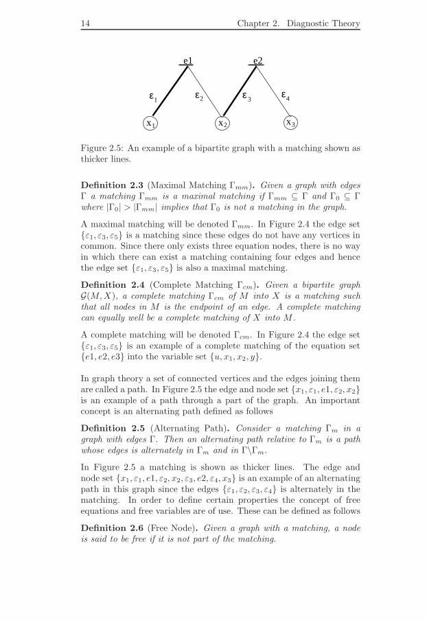
Figure 2.5: An example of a bipartite graph with a matching shown asthicker lines.
Definition 2.3 (Maximal Matching Γmm). Given a graph with edgesΓ a matching Γmm is a maximal matching if Γmm ⊆ Γ and Γ0 ⊆ Γwhere |Γ0| > |Γmm| implies that Γ0 is not a matching in the graph.
A maximal matching will be denoted Γmm. In Figure 2.4 the edge setε1, ε3, ε5 is a matching since these edges do not have any vertices incommon. Since there only exists three equation nodes, there is no wayin which there can exist a matching containing four edges and hencethe edge set ε1, ε3, ε5 is also a maximal matching.
Definition 2.4 (Complete Matching Γcm). Given a bipartite graphG(M, X), a complete matching Γcm of M into X is a matching suchthat all nodes in M is the endpoint of an edge. A complete matchingcan equally well be a complete matching of X into M .
A complete matching will be denoted Γcm. In Figure 2.4 the edge setε1, ε3, ε5 is an example of a complete matching of the equation sete1, e2, e3 into the variable set u, x1, x2, y.
In graph theory a set of connected vertices and the edges joining themare called a path. In Figure 2.5 the edge and node set x1, ε1, e1, ε2, x2is an example of a path through a part of the graph. An importantconcept is an alternating path defined as follows
Definition 2.5 (Alternating Path). Consider a matching Γm in agraph with edges Γ. Then an alternating path relative to Γm is a pathwhose edges is alternately in Γm and in Γ\Γm.
In Figure 2.5 a matching is shown as thicker lines. The edge andnode set x1, ε1, e1, ε2, x2, ε3, e2, ε4, x3 is an example of an alternatingpath in this graph since the edges ε1, ε2, ε3, ε4 is alternately in thematching. In order to define certain properties the concept of freeequations and free variables are of use. These can be defined as follows
Definition 2.6 (Free Node). Given a graph with a matching, a nodeis said to be free if it is not part of the matching.

2.4. Structural Models and their Properties 15
e1
e3
e2
en
xnx1 x2 x3 . . . .
M+
M −
M0
Equations, M
X0
X−
X +
Maximal Matching
Alternating Path
Free Equations
. . .
.
Unknown Variables, X
Figure 2.6: Schematic illustration of canonical decomposition on amodel M . The gray rectangles represent matrices that may containnon-zero variables whereas all the entries in the white area are zero.
The main objective in this thesis is, as mentioned before, to find equa-tion sets in a system that can be used in the construction of a diag-nosis system. By Definition 2.1 the redundant or overdetermined partof a model seems to be of special interest. There is in other words aneed to divide a model into different parts and in some way extractthe overdetermined one. In [8] it is proven that there always exists aunique structurally overdetermined part in a model, a way to obtainthis part called canonical decomposition is also presented. Canonicaldecomposition can be explained by the following definition
Definition 2.7 (Canonical Decomposition). Let Γmm be a maximalmatching in the bipartite graph G(M, varXM). Denote the equationnodes and variable nodes in Γmm with Mm and Xm respectively. Thenthe set of all equation nodes in M such that they are reachable via analternating path from M\Mm is the structurally overdetermined partM+. The structurally underdetermined set M− is the set of all equationnodes in M such that there is an alternating path from varXM\Xm.The remaining part of the model is the structurally justdetermined partdenoted M0. The structurally overdetermined, justdetermined and un-derdetermined variables are defined asX+ = varXM+,
16 Chapter 2. Diagnostic Theory
5
1 x3 x4x2
4εε3ε2ε1 ε
x
e1 e2 e4e3
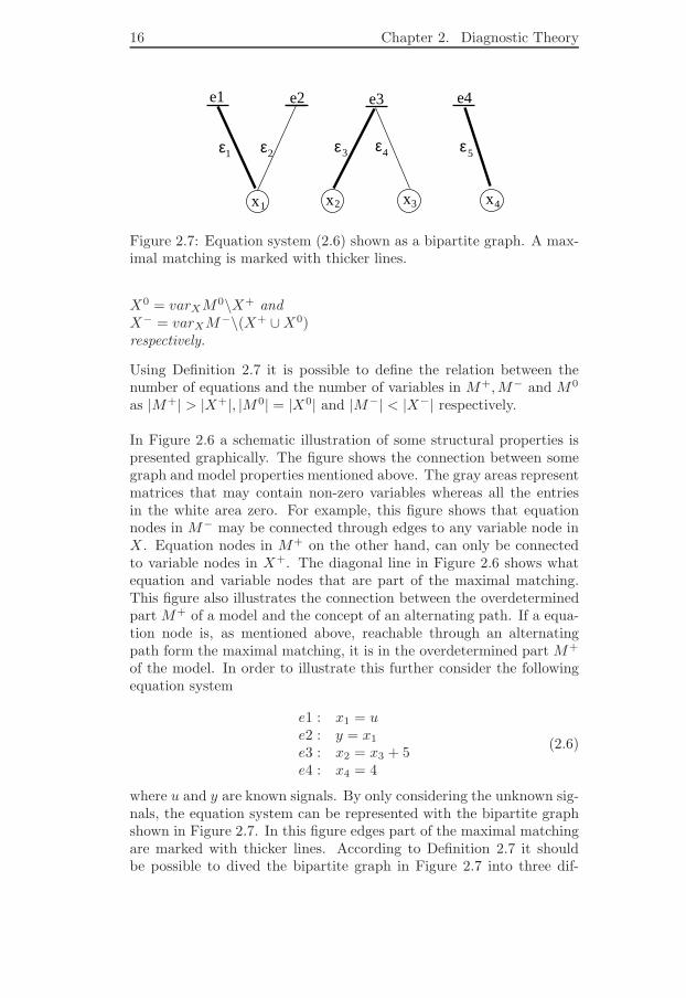
Figure 2.7: Equation system (2.6) shown as a bipartite graph. A max-imal matching is marked with thicker lines.
X0 = varXM0\X+ andX− = varXM−\(X+ ∪ X0)respectively.
Using Definition 2.7 it is possible to define the relation between thenumber of equations and the number of variables in M+, M− and M0
as |M+| > |X+|, |M0| = |X0| and |M−| < |X−| respectively.
In Figure 2.6 a schematic illustration of some structural properties ispresented graphically. The figure shows the connection between somegraph and model properties mentioned above. The gray areas representmatrices that may contain non-zero variables whereas all the entriesin the white area zero. For example, this figure shows that equationnodes in M− may be connected through edges to any variable node inX . Equation nodes in M+ on the other hand, can only be connectedto variable nodes in X+. The diagonal line in Figure 2.6 shows whatequation and variable nodes that are part of the maximal matching.This figure also illustrates the connection between the overdeterminedpart M+ of a model and the concept of an alternating path. If a equa-tion node is, as mentioned above, reachable through an alternatingpath form the maximal matching, it is in the overdetermined part M+
of the model. In order to illustrate this further consider the followingequation system
e1 : x1 = ue2 : y = x1
e3 : x2 = x3 + 5e4 : x4 = 4
(2.6)
where u and y are known signals. By only considering the unknown sig-nals, the equation system can be represented with the bipartite graphshown in Figure 2.7. In this figure edges part of the maximal matchingare marked with thicker lines. According to Definition 2.7 it shouldbe possible to dived the bipartite graph in Figure 2.7 into three dif-

2.4. Structural Models and their Properties 17
M
0
x1x4x2x3
M
+
M−x
x
e3e4e1e2
x
x
x
Figure 2.8: Equation system (2.6) divided into three parts by canonicaldecomposition. Variables and equations nodes included in the maximalmatching are marked with bigger x:s.
ferent parts. The overdetermined part is all equation nodes part of analternating path from equation nodes outside the maximal matching,i.e. equation nodes e1 and e2. The underdetermined part is all equa-tion nodes part of an alternating path from variable nodes outside themaximal matching, i.e. equation node e3. The justdetermined part isthe rest of the equation nodes in the graph, i.e. equation node e4. InFigure 2.8 this is shown in the same format as the system in Figure 2.6discussed above, variables and equations nodes included in the maxi-mal matching are marked with bigger x:s.
Since the redundant part of a model is the one used to construct di-agnostic tests, models that consist of only overdetermined parts areof special interest. Therefore it is convenient to make the followingdefinitions
Definition 2.8 (Structurally Overdetermined). An equation set M issaid to be Structurally Overdetermined (SO) if M = M+.
From Definition 2.7 and Definition 2.8 it follows that if M is SO thenM− = ∅ and M0 = ∅.
In the design of a diagnostic system small overdetermined models are ofspecial interest [7]. This follows from the fact that it is in general easierto construct residuals that are based on few equations and hence aresensitive to a few number of faults. One type of sets that are especiallyimportant in this sense, are Minimal Structurally Overdetermined setsor MSO sets. In fact in [7] it is shown that the problem of finding allparts of a model that can be used in order to construct residuals can,when using structural models, be reduced to finding all MSO sets (seeChapter 4). MSO sets are formally defined as follows
Definition 2.9 (Minimal Structurally Overdetermined). A structurallyoverdetermined set is a Minimal Structurally Overdetermined set (MSO)if none of its proper subsets are structurally overdetermined.

18 Chapter 2. Diagnostic Theory
An overdetermined equation system contains more equations then un-known variables. In order to make it easier to express how many moreequations then variables there is in such a system and hence define thedegree of redundancy, the following definition is convenient
Definition 2.10 (Degree of Overdeterminedness). The degree of overde-terminedness for an overdetermined set of equations M+ is defined as
n = |M+| − |varXM+| (2.7)
An overdetermined set of equation with a degree of overdeterminednessn will be denoted M+n, also called a +n system. For example, theoverdetermined part M+ in Figure 2.8 should be denoted M+1, sincethe set of equations in M+ got a degree of overdeterminedness equalto one.
Chapter 3
Algorithms for Simulink
At Scania, engine models are implemented in Simulink. In order tofind parts, i.e. equation sets, of a model that can be used to constructdiagnostic test there is a need, as mentioned before, to perform analyt-ical and structural computations on the model. Necessary calculationscan not however be performed directly in a Simulink model, since itis presented graphically. In this chapter some newly developed algo-rithms for handling analytical and structural transformations will bedescribed, as well as a method of inserting behavioral modes into aSimulink model. First in Section 3.1 a way of transforming a Simulinkmodel into analytical equations is introduced. Then in Section 3.2 thetransformation from analytical equations to a structural model is de-scribed. Finally in Section 3.3 a solution to the problem of includingbehavioral modes into a Simulink model is proposed.
3.1 Transforming Simulink Models to An-
alytical Equations
This section contains a description of an algorithm that retrieves allanalytical equations from a Simulink file. Since the engine models,treated in this thesis, are implemented in Simulink this is a necessarystep in the process of constructing a diagnostic system. The algorithmcan be summarized by the following steps.
Algorithm 3.1.
1. Simulink Simplification: Structuring the contents in the Simulinkfile in order to construct a less complex Simulink model.
2. Deriving Analytical Equations: Creates an analytical model fromthe structure given in step (1).
19

20 Chapter 3. Algorithms for Simulink
Constant
2
Display
2
Figure 3.1: Example of a Simulink file(simex.mdl).
3. Analytical Simplification: Simplifies the analytical model in orderto decrease the complexity of the system.
In step (1) the Simulink file is parsed and the important parts, i.e. partsthat contain analytical information, are extracted and transformed intoa less complex structure. Step (2) turns the structure created in step (1)into analytical equations. Finally in step (3) an analytical simplificationis made in order to reduce the size of the model. A more thoroughdescription of the individual steps in Algorithm 3.1 is given in thesections that follows.
3.1.1 Simulink Simplification
Simulink files are stored as text files. In order to decrease the timespent reading files, there is a need to transform these into a more com-prehensible format.
Example 3.1
The Simulink model in Figure 3.1 is in this example first shown asa text file and then transformed into a less complex object orientedstructure.
Model
Name "simex"
System
Name "simex"
Block
BlockType Constant
Name "Constant"
Value "2"
Block
BlockType Display

3.1. Transforming Simulink Models to Analytical Equations 21
Name "Display"
Ports [1]
Line
SrcBlock "Constant"
SrcPort 1
DstBlock "Display"
DstPort 1
By parsing the file above and extracting the different levels of classes,the model in the file can be transformed to the following, less complex,structure.
simex.Constant.Blocktype = Constant
simex.Constant.Name = "Constant"
simex.Constant.Value = "2"
simex.Display.Blocktype = Display
simex.Display.Name = "Display"
simex.Display.Ports = [1]
simex.Line.SrcBlock = Constant
simex.Line.SrcPort = 1
simex.Line.DstBlock = "Display"
simex.Line.DstPort = 1
As shown in Example 3.1, Simulink files are built hierarchical. Thismeans that they are on an ideal format to be transform into a sortof object oriented format, with super and subclasses. For example,if a Simulink block named sum is contained in a subsystem namedsubsystem1, then it is possible to transform these into a structure likesubsystem1.sum. Hence, an object oriented structure can easily becreated by parsing Simulink files and extracting blocks and lines as ex-plained by Example 3.1. By transforming Simulink files into structuresthe time spent reading files are minimized. Since file access is fairlytime demanding, the execution time is hence reduced.
3.1.2 Deriving Analytical Equations from Simulink
In a Simulink file signals are represented as lines (see Figure 3.1). Theselines are connected to blocks which, with some exceptions, execute a

22 Chapter 3. Algorithms for Simulink
3
++2
Constant
y
SensorTo Workspace
ActuatorFrom Workspace
u
S1
1
X
Product
Constant1
S2
1
S1 S2
Subsystem
a1
Subsystem
a4
a5
a3
sum
a2
Figure 3.2: Example Simulink model with a subsystem.
computation on the signals. This process coincide with the behaviorof a mathematical function, i.e. a block can be compared with a func-tion Y = f(X), where X is a vector of input signals and Y is a vectorwith output signals. Hence, by defining the analytical function f foreach block in a model it should be possible to convert the model intoan analytical equation system. If there, for example, exists a summa-tion block, e.g. sum in Figure 3.2, there must exist a definition thatthis block corresponds to equation S1 = a1 + a2. In this thesis thiswas solved by using a special definition file that contains the analyti-cal functions for all the block types needed. Another problem is thatSimulink models often contain unnamed lines. Since this correspondsto unnamed variables in the equation system, these need to be namedbefore they can be included into a model. This can however be solvedautomatically by the algorithm and causes no problem. The algorithmcan now be written as follows.
Algorithm 3.2.
Input: An object oriented structure S of a Simulink model given fromstep (1) in Algorithm 3.1.
1. Let B be the set of all blocks and L be the set of all lines in S.
2. For all unnamed lines in L assign a unique variable name.
3. Set i = 1.
4. Select block bi ∈ B.

3.1. Transforming Simulink Models to Analytical Equations 23
5. Let X be all input signal names and Y all output signal namesfor the signals connected to bi.
6. Get the analytical function f corresponding to the block type ofbi.
7. Save the analytical function for bi as Y = f(X) together with aunique equation name.
8. If |B| 6= i set i = i + 1 and goto step (4), otherwise exit.
Output: The analytical equations for the Simulink model given from S.
By applying Algorithm 3.2 on the Simulink model in Figure 3.2 thefollowing analytical equation system is obtained.
e1 Constant : a1 = 2
e2 Actuator From Workspace : a2 = u
e3 Sum : S1 = a1 + a2
e4 Sensor To Workspace : y = S2
e5 Subsystem.S1 : a4 = S1
e6 Subsystem.Constant1 : a3 = 3
e7 Subsystem.Product : a5 = a4 * a3
e8 Subsystem.S2 : S2 = a5
Note that in the equation system above the block names for the blockscorresponding to each equation are also shown.
Special Simulink Blocks
In order for the transformation toward an analytical system model tobe correct, some special feature blocks need to be defined. These blocksare listed below.
Subsytem Treated as container component. Do not have any blockfunction other then naming signals connected to its ports (see S1and S2 in Figure 3.2).
To Workspace Treated as sensor signal in the model if the blockname is tagged with the letters Sensor (see ”Sensor To Workspace”in Figure 3.2).
From Workspace Treated as actuator signal in the model if the blockname is tagged with the letters Actuator (see ”Actuator FromWorkspace” in Figure 3.2).
The sensor and actuator blocks are important since they indicate signalswhich are considered known in the model. This information is laterused when transforming the analytical model into a structural model(see Section 3.2).

24 Chapter 3. Algorithms for Simulink
3.1.3 Analytical Simplification
Structural methods can be an efficient tool when trying to find parts ofa model that can be used to construct diagnostic tests (see Chapter 4).This must be kept in mind if an analytical model is simplified, other-wise structural information may be lost. By examining the analyticalequations generated by Algorithm 3.2 above, it can be seen that it ispossible to simplify analytically. For example, a5 can easily be elimi-nated by replacing it with S2 and hence can equation e8 be removed.The problem that arises when doing this is to not merge equations thatcan appear in different residuals. If this is done, information will belost and it may be impossible to structurally generate all possible testsfor a model. For example, consider the following analytical model.
e1 : y1 = x1
e2 : y2 = x2
e3 : x1 = x2
e4 : x1 = u
(3.1)
where y1, y2 and u are considered to be known variables. By doing acorrect, in the analytical sense, simplification this model can be reducedto
e1, e4 : y1 = ue2, e3, e4 : y2 = u
(3.2)
For (3.1) it is possible to structurally extract three residuals r1 = y1−u,r2 = y2 − u and r3 = y1 − y2. However, from the ”correct” simplifiedmodel it is only possible to structurally construct two residuals as r1 =y1−u and r2 = y2−u, hence one residual will be lost. This follows fromthe fact that the structural methods used in this thesis do not allowknown variables to be eliminated. The solution to this problem is tojust remove simple assignments of unknown variables from analyticalequation systems. By doing this, the model can be reduced withoutcausing the loss of structural information. For example consider themodel in (3.1). By letting x1 = x2 and then replace any occurrence ofx1 with x2 the model can be reduced to
e1 : y1 = x2
e2 : y2 = x2
e3 : x2 = x2
e4 : x2 = u
(3.3)
and hence, equation e3 can be removed without causing any informationloss. In test runs this reduced an engine model with approximately 360equations to about 170 equations. This will later on be proven to beextremely vital since the processing cost for finding residuals is highlydependent on the model size (see Chapter 4).

3.2. Structural Transformation 25
3.2 Structural Transformation
Earlier in Section 2.4 it was mentioned that by trying to find residualsin a structural model instead of in an analytical model, the compu-tation time could be significantly reduced. Hence it is essential thatequations derived from the Simulink model can be transformed to theirstructural form. However, this is not difficult since the only informa-tion that should be included is which variables each equation containsand if they are consided to be known or unknown.
The analytical equations for the system in Figure 3.2 was presentedin Section 3.1.2. Now the equations can be transformed to the follow-ing structural model.
equations unknown knowna1 a2 a3 a4 a5 S1 S2 u y
e1 xe2 x xe3 x x xe4 x xe5 x xe6 xe7 x x xe8 x x
As mentioned in Section 3.1.2, Sensor tagged To Workspace and Ac-tuator tagged From Workspace blocks are treated as known signals.Hence variable u and y are shown as known variables in the structuralmodel.
3.3 Behavioral Modes in Simulink
The main objective in this thesis is to extract equations from a modelthat later can be used to construct diagnostic tests. As explained inSection 2.2 and 2.3 the use of fault models and behavioral modes in amodel may increase the possibility for the diagnostic systems to isolatefaults, and hence increase the diagnostic performance. Since the modelsconsidered in this thesis are implemented in Simulink, which is basedon a graphical interface, it would be preferred if the behavioral modescan be included directly in the visual model. This section describes ageneral solution of how this can be done without changing the modelappearance significantly. Note that there is a difference between faultsimulation and fault modeling in Simulink. Since the Simulink meth-

26 Chapter 3. Algorithms for Simulink
Actuator
u
Sensor
y
Figure 3.3: Example of a Simulink model.
ods described in this thesis only focus on extracting equations fromSimulink models, there is no guarantee that the fault model solutionsdescribed in this section can run under a Simulink simulation. How-ever, the method proposed in this section has been developed with thisin mind and a solution to the simulation problem will not be hard toobtain.
3.4 Fault Modeling in Simulink
When modeling faults graphically in Simulink, enough informationmust be included into the model so it is possible to extract all behav-ioral modes. For example, consider the Simulink model in Figure 3.3.The corresponding model can be written as
y = u (3.4)
where y is a sensor measuring the signal u. Assume now that thesensor has three possible fault models: a constant bias fault (B), ashort circuit (SC) and some unknown faults (UF). Let Ω denote the setof all behavioral modes in the system as Ω = NF, B, SC, UF whereNF denotes the No Fault mode. An example of how this model maylook like can be written as follows.
Ass. EquationNF y = uB y = u + bSC y = 0UF y ∈ RΩ b = 0
(3.5)
where Ass. is the behavioral mode assumption. If the system behaviordiverge for any equation above the conclusion is that the system is notin the corresponding behavioral mode. For example, if u 6= 0 and y = 0then the conclusion will be that that the system is not in the faultfree NF state. In order to introduce systems like (3.5) into a Simulinkmodel there must first be a way to include this information graphi-cally. Algorithm 3.2, that transforms Simulink models into analyticalequations must be modified in order to connect the right equations to
3.4. Fault Modeling in Simulink 27
++Actuator
u
Sensor
y
NF
B
SC
UF>
0
F2
UK F1
b
BM C1
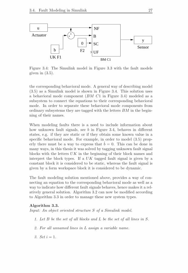
Figure 3.4: The Simulink model in Figure 3.3 with the fault modelsgiven in (3.5).
the corresponding behavioral mode. A general way of describing model(3.5) as a Simulink model is shown in Figure 3.4. This solution usesa behavioral mode component (BM C1 in Figure 3.4) modeled as asubsystem to connect the equations to their corresponding behavioralmode. In order to separate these behavioral mode components fromordinary subsystems they are tagged with the letters BM in the begin-ning of their names.
When modeling faults there is a need to include information abouthow unknown fault signals, see b in Figure 3.4, behaves in differentstates, e.g. if they are static or if they obtain some known value in aspecific behavioral mode. For example, in order to model (3.5) prop-erly there must be a way to express that b = 0. This can be done inmany ways, in this thesis it was solved by tagging unknown fault signalblocks with the letters UK in the beginning of their block names andinterpret the block types. If a UK tagged fault signal is given by aconstant block it is considered to be static, whereas the fault signal isgiven by a form workspace block it is considered to be dynamic.
The fault modeling solution mentioned above, provides a way of con-necting an equation to the corresponding behavioral mode as well as away to indicate how different fault signals behaves, hence makes it a rel-atively general solution. Algorithm 3.2 can now be modified accordingto Algorithm 3.3 in order to manage these new system types.
Algorithm 3.3.
Input: An object oriented structure S of a Simulink model.
1. Let B be the set of all blocks and L be the set of all lines in S.
2. For all unnamed lines in L assign a variable name.
3. Set i = 1.
28 Chapter 3. Algorithms for Simulink
4. Select block bi ∈ B.
5. Let X be all input signal names and Y all output signal namesfor the signals connected to bi.
6. If bi is a constant block tagged with the letters UK giving a signalθ, save θ′ = 0 as an analytical function together with a uniqueequation name.
7. If not bi is a subsystem tagged with the letters BM goto step (9).
8. For all x ∈ X save x = Y as an analytical function together witha unique equation name and the behavioral mode name given frombi, then goto step (11).
9. Get the analytical function f corresponding to the block type ofbi.
10. Save the analytical function for bi as Y = f(X) together with aunique equation name.
11. If |B| 6= i set i = i + 1 and goto step (4) otherwise exit.
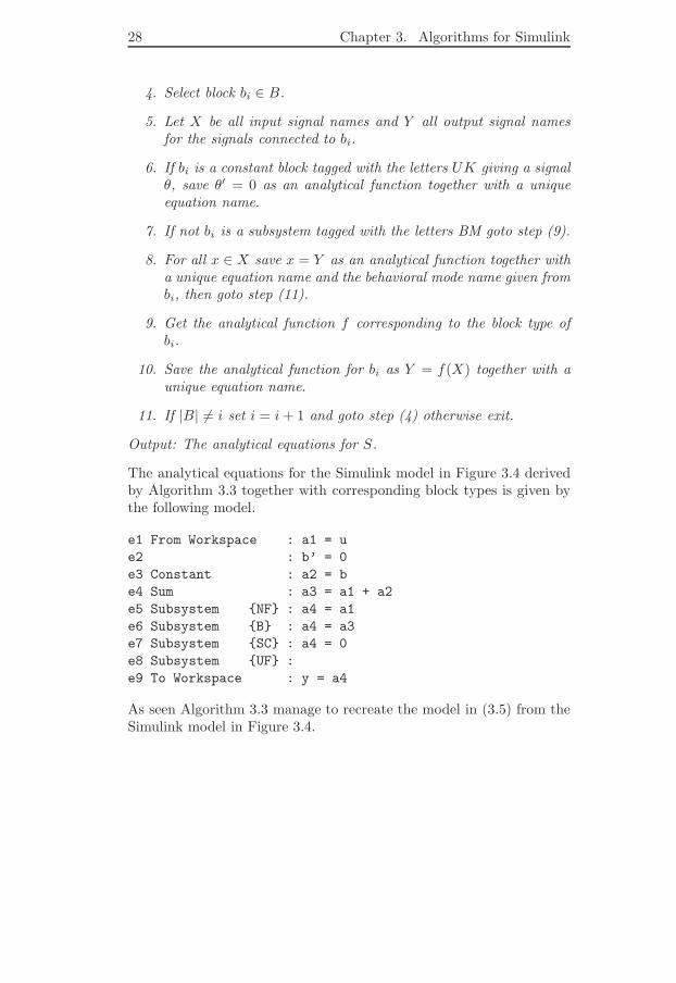
Output: The analytical equations for S.
The analytical equations for the Simulink model in Figure 3.4 derivedby Algorithm 3.3 together with corresponding block types is given bythe following model.
e1 From Workspace : a1 = u
e2 : b’ = 0
e3 Constant : a2 = b
e4 Sum : a3 = a1 + a2
e5 Subsystem NF : a4 = a1
e6 Subsystem B : a4 = a3
e7 Subsystem SC : a4 = 0
e8 Subsystem UF :
e9 To Workspace : y = a4
As seen Algorithm 3.3 manage to recreate the model in (3.5) from theSimulink model in Figure 3.4.

Chapter 4
Structural Algorithms
As explained in Chapter 2, minimal structurally overdetermined setsare of special interest when designing diagnostic tests, since they arein general small and sensitive to few faults. In [7], it is shown thatby using the MSO sets contained in a model it is possible to constructsufficiently accurate diagnostic system. Hence, in order to constructa solid diagnostic system, just using structural models, it is essentialthat all MSO sets are found. In [7], an algorithm for extracting allMSO sets from a system model is presented. However, some of thesteps in this algorithm are highly ineffective and computational ex-pensive for the kind of models considered in this thesis. This chapterpresents newly developed algorithms for extracting all MSO sets con-tained in a structural model. In Section 4.1 the main objectives forthe new algorithm are given. In Section 4.2 and 4.3 a more detaileddescription of the different steps in the algorithm are presented. InSection 4.4 a partially changed algorithm for finding all MSO sets ina system containing behavioral modes is shown. Finally in Section 4.5the correctness of the new algorithms is proved. The input to all thesealgorithms is a structural model extracted from the model equations ofthe engine, see Section 3.2.
4.1 Steps Toward Finding All MSO Sets
In [7] Algorithm 8.1 introduces a way of finding all MSO sets in astructural model. In this section a new improved and partially changedversion of this algorithm is presented. The algorithm can be describedby the following structure
29

30 Chapter 4. Structural Algorithms
Algorithm 4.1.
Input: A structural model M.
1. Removing derivatives: This algorithm does not separate a vari-able from its derivatives, hence the structural model M must betransformed to a DLSM (see Section 2.4.1).
2. Extracting the overdetermined part of the model: Since MSOs cannot contain any justdetermined or underdetermined parts, theseare removed (see Definition 2.8 and Definition 2.9).
3. Structural Simplification: Simplifies the model by combining equa-tion sets that have to be used together in an MSO set. This pro-duces a less complex model, fewer equations and unknown vari-ables, and hence decreases the computing time in the next step.
4. Finding all MSO sets: Searching the structural model obtainedfrom the last step and extracting all MSO sets.
Output: All MSO sets contained in the model M.
As mentioned above Algorithm 4.1 is a modified version of an algorithmpresented in [7]. However the results given from the two algorithms arethe same. Compared to the algorithm in [7] it is mainly step (3) andstep (4) of Algorithm 4.1 that have been improved. Hence, in thefollowing sections a more thorough description of these steps will begiven. For more information concerning the other steps see [7].
4.2 Structural Simplification
As mentioned earlier in Section 2.4, finding all diagnostic tests for amodel is a complex task. This is still the case when using structuralmethods. Hence every simplification of the structural model is helpful.In [7] a structural simplification algorithm is introduced. The algorithmcreates a simpler model by merging those equations that must be in thesame MSO. The merging is achieved by looking for unknown variablesthat are present in only two equations. If such a variable is found thetwo equations are combined and the variable is removed. This can bedescribed according to the following
Algorithm 4.2.
Input: A structural overdetermined model M ′
1. Set X ′ = varXM ′.
2. For all variables x ∈ X ′ do step (3).

4.2. Structural Simplification 31
3. If |equM ′x| = 2 merge the equations in equM ′x and remove thevariable x.
4. If any equations was merged in step (3) goto step (1) otherwiseexit.
Output: The simplified model M ′.
This algorithm can be illustrated through a simple example. Considerthe following analytical equation system
e1 : y1 = x1 + u1
e2 : y2 = x1 + u2(4.1)
where the variables yi and ui are known while x1 are unknown. In thiscase the unknown variable x1 is present in only two equations. Hence,according to the Algorithm 4.2 the two equations can be merged andthe variable x1 removed. By doing this the following equation systemis derived
e1, e2 : y1 − y2 = u1 − u2 (4.2)
The algorithm repeats these steps until no more simplification is pos-sible. By applying this on structural models it produces an effectivesimplification. However Algorithm 4.2 is not able to handle all struc-tural cases. Consider the structural model describing an MSO in Table4.1. In the first run with Algorithm 4.2 variable x3 is found to bepresent in only two equations, e3 and e4. Hence x3 is removed andequations e3 and e4 merged together. The result is shown in Table4.2. Since there not exists any more variables contained in only twoequations Algorithm 4.2 will now exit.
equation unknown knownx1 x2 x3 y u
e1 x x xe2 x x xe3 x x x xe4 x x
Table 4.1: An example of a structural model before the simplificationstep.
In Table 4.1 all equations can be merged together since all equationsis needed to remove the unknown variables in the system, and hencemust be used together in an MSO. However, Table 4.2 clearly showsthat Algorithm 4.2 fails to find all possible ways of merging equationsand simplifying the model. This problem can be solved by construct-ing a new simplification algorithm that uses the properties of canonical
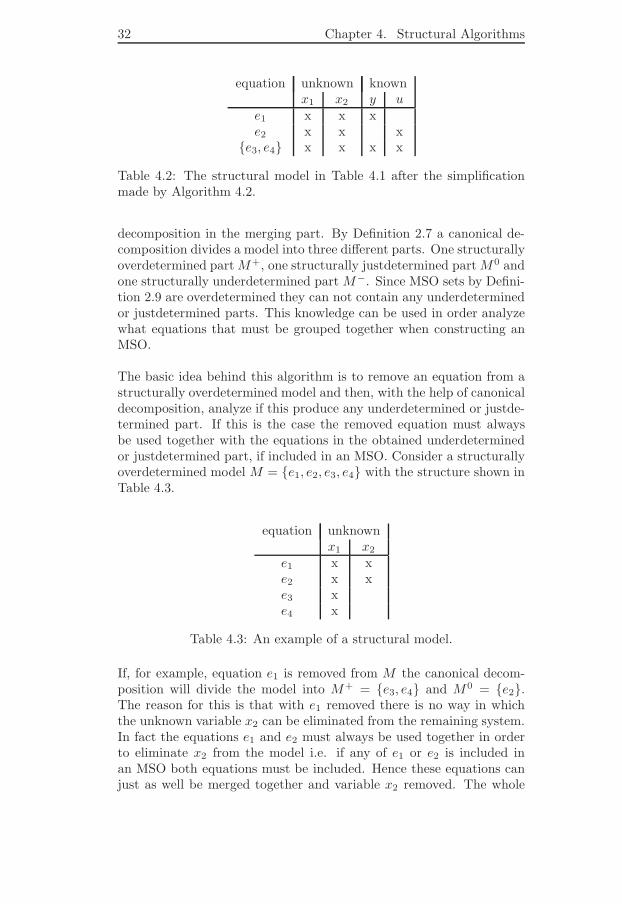
32 Chapter 4. Structural Algorithms
equation unknown knownx1 x2 y u
e1 x x xe2 x x x
e3, e4 x x x x
Table 4.2: The structural model in Table 4.1 after the simplificationmade by Algorithm 4.2.
decomposition in the merging part. By Definition 2.7 a canonical de-composition divides a model into three different parts. One structurallyoverdetermined part M+, one structurally justdetermined part M0 andone structurally underdetermined part M−. Since MSO sets by Defini-tion 2.9 are overdetermined they can not contain any underdeterminedor justdetermined parts. This knowledge can be used in order analyzewhat equations that must be grouped together when constructing anMSO.
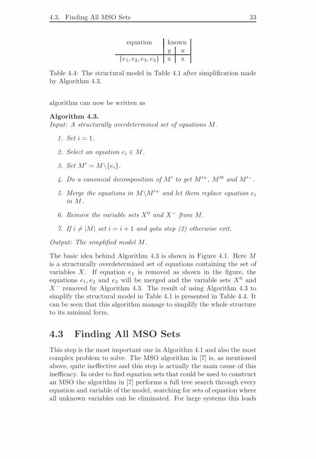
The basic idea behind this algorithm is to remove an equation from astructurally overdetermined model and then, with the help of canonicaldecomposition, analyze if this produce any underdetermined or justde-termined part. If this is the case the removed equation must alwaysbe used together with the equations in the obtained underdeterminedor justdetermined part, if included in an MSO. Consider a structurallyoverdetermined model M = e1, e2, e3, e4 with the structure shown inTable 4.3.
equation unknownx1 x2
e1 x xe2 x xe3 xe4 x
Table 4.3: An example of a structural model.
If, for example, equation e1 is removed from M the canonical decom-position will divide the model into M+ = e3, e4 and M0 = e2.The reason for this is that with e1 removed there is no way in whichthe unknown variable x2 can be eliminated from the remaining system.In fact the equations e1 and e2 must always be used together in orderto eliminate x2 from the model i.e. if any of e1 or e2 is included inan MSO both equations must be included. Hence these equations canjust as well be merged together and variable x2 removed. The whole
4.3. Finding All MSO Sets 33
equation knowny u
e1, e2, e3, e4 x x
Table 4.4: The structural model in Table 4.1 after simplification madeby Algorithm 4.3.
algorithm can now be written as
Algorithm 4.3.
Input: A structurally overdetermined set of equations M .
1. Set i = 1.
2. Select an equation ei ∈ M .
3. Set M ′ = M\ei.
4. Do a canonical decomposition of M ′ to get M ′+, M ′0 and M ′−.
5. Merge the equations in M\M ′+ and let them replace equation ei
in M .
6. Remove the variable sets X0 and X− from M .
7. If i 6= |M | set i = i + 1 and goto step (2) otherwise exit.
Output: The simplified model M .
The basic idea behind Algorithm 4.3 is shown in Figure 4.1. Here Mis a structurally overdetermined set of equations containing the set ofvariables X . If equation e1 is removed as shown in the figure, theequations e1, e2 and e3 will be merged and the variable sets X0 andX− removed by Algorithm 4.3. The result of using Algorithm 4.3 tosimplify the structural model in Table 4.1 is presented in Table 4.4. Itcan be seen that this algorithm manage to simplify the whole structureto its minimal form.
4.3 Finding All MSO Sets
This step is the most important one in Algorithm 4.1 and also the mostcomplex problem to solve. The MSO algorithm in [7] is, as mentionedabove, quite ineffective and this step is actually the main cause of thisinefficacy. In order to find equation sets that could be used to constructan MSO the algorithm in [7] performs a full tree search through everyequation and variable of the model, searching for sets of equation whereall unknown variables can be eliminated. For large systems this leads
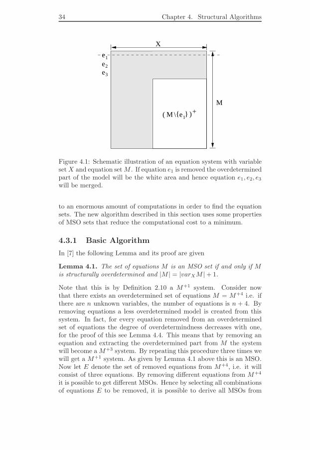
34 Chapter 4. Structural Algorithms
1
e2
e3
e1M \ +)(
e
X
M
Figure 4.1: Schematic illustration of an equation system with variableset X and equation set M . If equation e1 is removed the overdeterminedpart of the model will be the white area and hence equation e1, e2, e3
will be merged.
to an enormous amount of computations in order to find the equationsets. The new algorithm described in this section uses some propertiesof MSO sets that reduce the computational cost to a minimum.
4.3.1 Basic Algorithm
In [7] the following Lemma and its proof are given
Lemma 4.1. The set of equations M is an MSO set if and only if Mis structurally overdetermined and |M | = |varXM | + 1.
Note that this is by Definition 2.10 a M+1 system. Consider nowthat there exists an overdetermined set of equations M = M+4 i.e. ifthere are n unknown variables, the number of equations is n + 4. Byremoving equations a less overdetermined model is created from thissystem. In fact, for every equation removed from an overdeterminedset of equations the degree of overdetermindness decreases with one,for the proof of this see Lemma 4.4. This means that by removing anequation and extracting the overdetermined part from M the systemwill become a M+3 system. By repeating this procedure three times wewill get a M+1 system. As given by Lemma 4.1 above this is an MSO.Now let E denote the set of removed equations from M+4, i.e. it willconsist of three equations. By removing different equations from M+4
it is possible to get different MSOs. Hence by selecting all combinationsof equations E to be removed, it is possible to derive all MSOs from

4.3. Finding All MSO Sets 35
M+4. This can be formalized by the algorithm that follows below. Theinput to this algorithm is the simplified model derived by Algorithm4.3.
Algorithm 4.4.
Input: A structurally overdetermined set of equations M+n = e1, .., en.
1. Set i = 1.
2. Select an equation ei ∈ M+n.
3. Let M+(n−1) = (M+n\ei)+ .
4. If n − 1 6= 1 call this algorithm with M+(n−1).
5. If n − 1 = 1 save M+(n−1) as an MSO.
6. If i 6= |M+n| set i = i + 1 and goto step (2) otherwise exit.
Output: All MSO sets in M+n.
Algorithm 4.4 performs a systematical reduction of the equation setM+n until all M+1 systems are derived. Step (2) chooses an equationfrom M+n that is used in step (3) to decrease the degree of overde-terminedness n with one. The equation set obtained is according toDefinition 2.10 a +(n − 1) system, hence the chosen notation M+n−1.If an MSO is derived it is saved and the algorithm chooses the nextequation in the set, otherwise the algorithm calls itself with the newM+(n−1) system. In Example 4.1 a run with this algorithm is shown.
Example 4.1
Consider the following structurally overdetermined model consistingof four equations and two unknown variables
equation unknownx1 x2
e1 xe2 x xe3 xe4 x
Input to the algorithm: M+2 = e1, e2, e3, e4
36 Chapter 4. Structural Algorithms
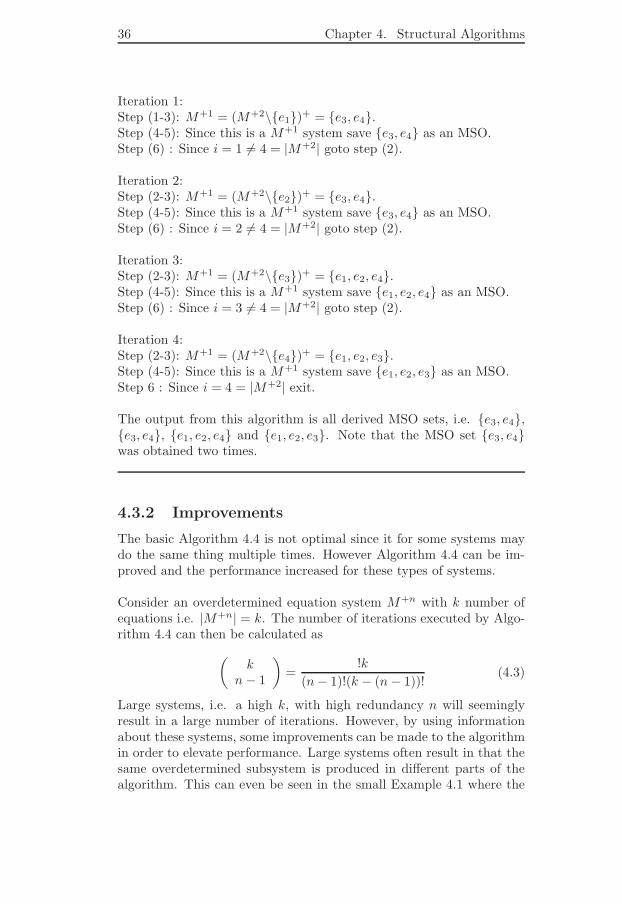
Iteration 1:Step (1-3): M+1 = (M+2\e1)+ = e3, e4.Step (4-5): Since this is a M+1 system save e3, e4 as an MSO.Step (6) : Since i = 1 6= 4 = |M+2| goto step (2).
Iteration 2:Step (2-3): M+1 = (M+2\e2)+ = e3, e4.Step (4-5): Since this is a M+1 system save e3, e4 as an MSO.Step (6) : Since i = 2 6= 4 = |M+2| goto step (2).
Iteration 3:Step (2-3): M+1 = (M+2\e3)+ = e1, e2, e4.Step (4-5): Since this is a M+1 system save e1, e2, e4 as an MSO.Step (6) : Since i = 3 6= 4 = |M+2| goto step (2).
Iteration 4:Step (2-3): M+1 = (M+2\e4)+ = e1, e2, e3.Step (4-5): Since this is a M+1 system save e1, e2, e3 as an MSO.Step 6 : Since i = 4 = |M+2| exit.
The output from this algorithm is all derived MSO sets, i.e. e3, e4,e3, e4, e1, e2, e4 and e1, e2, e3. Note that the MSO set e3, e4was obtained two times.
4.3.2 Improvements
The basic Algorithm 4.4 is not optimal since it for some systems maydo the same thing multiple times. However Algorithm 4.4 can be im-proved and the performance increased for these types of systems.
Consider an overdetermined equation system M+n with k number ofequations i.e. |M+n| = k. The number of iterations executed by Algo-rithm 4.4 can then be calculated as
(
kn − 1
)
=!k
(n − 1)!(k − (n − 1))!(4.3)
Large systems, i.e. a high k, with high redundancy n will seeminglyresult in a large number of iterations. However, by using informationabout these systems, some improvements can be made to the algorithmin order to elevate performance. Large systems often result in that thesame overdetermined subsystem is produced in different parts of thealgorithm. This can even be seen in the small Example 4.1 where the

4.3. Finding All MSO Sets 37
1
c3c2c1
b1 b2
an
n−1
n−2
overdetermindnessDegree of
Figure 4.2: A part of an execution with Algorithm 4.4 represented asa tree, where each node represents a set of equations M+n.
MSO e3, e4 was derived two times. Figure 4.2 describes a run withthe algorithm presented as an execution tree, where each node repre-sents a set of equations M+n. Assume now that the equation set b1 inthe left most path is the same as b2 in the right most path in Figure4.2. Since these are the same it is obvious that they will result in thesame children in the execution tree, in this case c1, c2 and c3. Hence,it is unnecessary to continue the execution in the right path after nodeb2. This can be solved by keeping track of the equation sets producedat each level in the tree and hence avoid any identical execution.
Another improvement uses the same principle as the new structuralsimplification step described in section 4.2. In step (3) of Algorithm 4.4,an equation ei is removed and a new overdetermined part is extractedas
M+(n−1) = (M+n\ei)+ (4.4)
Let E = M+(n−1)\M+n. According to Lemma 4.6 an equivalent E willbe derived as long as ei ∈ E in (4.4). Hence, it is unnecessary to selectmore than one equation ei ∈ E, since this will produce the same re-sult. By keeping track of equations that will produce equivalent resultsin step (3) of Algorithm 4.4 the number of iterations will be reduced.This simplification step uses the same theory as the structural simpli-fication Algorithm 4.3. Hence, there is no need to do any structuralsimplification before this new improved MSO algorithm is executed.

38 Chapter 4. Structural Algorithms
Let Mso be a set containing structurally overdetermined equation sets,the improved algorithm will then look as follows.
Algorithm 4.5.
Input: A structurally overdetermined set of equations M+n = e1, .., en..
1. Mso = ∅.
2. Let E = M+n.
3. Select an equation e ∈ E.
4. Let M+(n−1) = (M+n\e)+ .
5. Set E = E\(M+n\M+(n−1)).
6. If M+(n−1) already exists in Mso goto step (3) otherwise letMso = Mso ∪ Mn−1.
7. If n − 1 6= 1 call this algorithm with M+(n−1).
8. If n − 1 = 1 save M+(n−1) as an MSO.
9. If E 6= ∅ goto step (2) otherwise exit.
Output: All MSO sets in M+n.
In Example 4.2 a run with Algorithm 4.5 on the same model as in Ex-ample 4.1 is shown.
Example 4.2
Consider the structurally overdetermined model in Example 4.1 again.
equation unknownx1 x2
e1 xe2 x xe3 xe4 x
Input to the algorithm: M+2 = e1, e2, e3, e4

4.4. Finding All MSO Sets in a Behavioral Mode System 39
Iteration 1:Step (1) : E = e1, e2, e3, e4.Step (2) : Select an equation from E = e1, e2, e3, e4.Step (3) : M+1 = (M+2\e1)+ = e3, e4.Step (4) : E = E\(M+2\e3, e4) = e3, e4.Step (5) : Since M+1 has not been obtained earlier goto step (6).Step (6-7): Since this is a M+1 system save e3, e4 as an MSO.Step (8) : Since E 6= ∅ goto step (2).
Iteration 2:Step (2) : Select an equation from E = e3, e4.Step (3) : M+1 = (M+2\e3)+ = e1, e2, e4.Step (4) : E = E\(M+2\e1, e2, e4) = e4.Step (5) : Since M+1 has not been obtained earlier goto step (6).Step (6-7): Since this is a M+1 system save e1, e2, e4 as an MSO.Step (8) : Since E 6= ∅ goto step (2).
Iteration 3:Step (2) : Select an equation from E = e4.Step (3): M+1 = (M+2\e4)+ = e1, e2, e3.Step (4) : E = E\(M+2\e1, e2, e3) = .Step (5) : Since M+1 has not been obtained earlier goto step (6).Step (6-7): Since this is a M+1 system save e1, e2, e3 as an MSO.Step (8) : Since E = ∅ exit.
The output from this algorithm is all derived MSO sets, i.e. e3, e4,e1, e2, e4 and e1, e2, e3.
As seen in Example 4.2 Algorithm 4.5 manage to avoid the doubleexecution made by Algorithm 4.5 in Example 4.1. The number ofiterations is, in this example, reduced with 25%. In larger models theimprovements in Algorithm 4.5 shows to have an even bigger impacton the number of iterations and hence reduces the execution timesdramatically (see Chapter 5).
4.4 Finding All MSO Sets in a Behavioral
Mode System
The insertion of behavioral modes into a model is not uncomplicated.New problems arise such as increased execution time and the produc-tion of invalid MSO sets. As explained in Section 3.3, behavioral modesin this thesis appear in a system model as new equations, i.e. each be-

40 Chapter 4. Structural Algorithms
+
x1
yNF
B5
0 SC
Figure 4.3: Example of a behavioral mode component.
havioral mode correspond to one equation in the system model. Forexample, the behavioral mode component shown in Figure 4.3 can betranslated into
NF : y = x1
B : y = x1 + 5SC : y = 0
(4.5)
Equations connected to a specific behavioral mode component, like theones in (4.5), are supposed to be valid in separate fault modes. If forexample the component in Figure 4.3 is in a fault free environmentthe first equation in (4.5) is valid, whereas if the component got a biasfault of 5 the second equation is the correct one. This means thatthere should not be possible to include two or more equations from thesame behavioral mode component in an MSO. In the present form theMSO Algorithm 4.5 does not prevent this. Hence, it will produce someinvalid MOS sets if it is executed on a model, containing behavioralmodes equations like (4.5). This can easily be solved by simply re-moving all invalid MSO sets after the algorithm has finished. However,since new equations containing the same variables are included into themodel, when new behavior modes are added, this will make the modelmore redundant. As explained in Section 4.3.2 the number of iterationsperformed by Algorithm 4.5 is highly dependent on the redundancy ofthe system. Introducing behavioral modes into the system will causethe execution time to increase significantly. This problem is solved bytagging the equations connected to a specific behavioral mode compo-nent with the name of that behavioral mode component. Algorithm 4.5can then be modified to disallow two equations with identical tags tobe included into the same MSO. Let equCi
(M+n) be the equations ina structurally overdetermined set of equations M+n tagged with thebehavioral mode component Ci. Note that this is an extension of theequX(M) notation motioned earlier. The modified version of Algo-rithm 4.5 can then be written as follows.
Algorithm 4.6.
Input: A structural overdetermined set of equations M+n.
1. If there exists any i such that |equCi(M+n)| > 1 select one such
Ci and let E = equCi(M+n), else let E = M+n.
4.5. The Correctness of the Algorithms 41
2. Select an equation e ∈ E.
3. Let M+(n−1) = (M+n\e)+ .
4. Set E = E\(M+n\M+(n−1)).
5. If M+(n−1) already exist in the MSO-structure goto step (2).
6. If n − 1 6= 1 call this algorithm with M+(n−1).
7. If n− 1 = 1 and there not exists any i such that |equCiM+n| > 1
save M+(n−1) as an MSO.
8. If E 6= ∅ goto step (2).
Output: All MSO sets in M+n.
In Algorithm 4.6 step (1), (2) and (8) have been changed or added incomparison to Algorithm 4.5. Step (1) and (2) checks if there are twoor more equations with identical behavioral mode component tags inthe model. If this is the case one of these equations is removed. Due tothe systematical reduction of the model this will lead to that every pos-sible combination of behavioral mode equations will be included in theMSOs as long as there never is more than one with a specific tag. Notethat Algorithm 4.6 is not general since it assumes that all behavioralmodes can be expressed with one equation. This may not necessarilybe the case when concerning models not generated thought the algo-rithms described in this thesis. However, Algorithm 4.6 can easily beextended to handle all model types. Algorithm 4.6 shows to be effectiveeven in highly redundant behavioral mode systems. Test runs of largeengine models containing behavioral modes, shows that Algorithm 4.6finds all MSO sets more than ten times faster than Algorithm 4.5.
The algorithms presented in this chapter require some new propertiesof structural models that has not previously been proved. In the fol-lowing section some newly developed lemmas and proofs are presentedin order to analyze the correctness of the algorithms. This part of thethesis is however quite theoretical and is possible to omit.
4.5 The Correctness of the Algorithms
In order to prove the correctness of Algorithm 4.1, in particular thethe simplification step described in Section 4.2 (see Lemma 4.6) andthe MSO algorithm presented in Section 4.3 (see Theorem 4.1), a fewsupporting lemmas need to be defined.

42 Chapter 4. Structural Algorithms
The following lemma provides a connection between the matching prop-erty of bipartite graphs and structurally overdetermined models, seeSection 2.4.
Lemma 4.2. If an equation set M is structurally overdetermined thenthere exists a complete matching Γcm of varXM into M inG(M, varXM).
Proof. Consider a structurally overdetermined set of equations M andassume that there is no complete matching of varXM into M inG(M, varXM). Now for any maximal matching Γmm in G(M, varXM)there must exist a free variable vertex v. Then for all e ∈ equM(v) apath P (v, e) is an alternating path in G(M, varXM). Hence by Defin-ition 2.7 it follows that e ∈ M−, i.e. M− 6= ∅. According to Definition2.8 this contradicts the assumption that M is structurally overdeter-mined.
In the next lemma an important consequence of structurally overdeter-mined equation sets is given
Lemma 4.3. Let M be a set of equations. If M ′ ⊆ M is an SO modelthen M ′ ⊆ M+.
Proof. Consider an arbitrary structurally overdetermined set of equa-tions M ′ ⊆ M . From Lemma 4.2 it follows that there must exist acomplete matching Γcm of varXM ′ into M ′ in G(M ′, varXM ′). Thismeans that equ(Γcm) ⊆ M ′ and var(Γcm) ⊆ varXM ′. Set X ′ =varXM\varXM ′ and let Γmm be a maximum matching in G(M\M ′, X ′).Then it follows that equ(Γmm) ⊆ (M\M ′) and var(Γmm) ⊆ X ′. Fromthe definition of X ′ this gives that X ′ ∩ varXM ′ = ∅ which impliesthat var(Γcm) ∩ var(Γmm) = ∅, i.e. the node sets of Γcm and Γmm
are disjunct. From this it follows that Γcm ∪ Γmm will be a match-ing in G(M, varXM). Since varX′M ′ = ∅ and Γcm is maximal inG(M ′, varXM ′) and Γmm is maximal in G(M\M ′, X ′), this impliesthat Γcm ∪ Γmm will be a maximal matching in G(M, varXM).
Now take an arbitrary equation e ∈ M ′. From Definition 2.8 and giventhat Γcm is a maximal matching in G(M ′, varXM ′), it follows that theremust exist an alternating path P in G(M ′, varXM ′) between e and afree equation e′ ∈ M ′. From Definition 2.7 and given that Γcm ∪ Γmm
is a maximal matching in G(M, varXM), this also implies that P willbe an alternating path in G(M, varXM). Furthermore since e′ ∈ M ′
is a free equation in G(M ′, varXM ′) w.r.t. Γcm and given that thenode sets of Γcm and Γmm are disjunct, it follows that e′ is also a freeequation w.r.t. Γcm∪Γmm in G(M, varXM). From this, the propertiesof P and Definition 2.7 it follows that e ∈ M+. Since e was arbitrary
4.5. The Correctness of the Algorithms 43
chosen this implies that every equation in M ′ is a part of M+ andhence M ′ ⊆ M+.
One of the most important features in Algorithm 4.4 is included in step(3), namely if one equation is removed from a structural overdeterminedset of equations, the degree of overdeterminedness will decrease withexactly one. This is formalized by the following lemma
Lemma 4.4. If M is a structurally overdetermined set of equationswith the degree of overdeterminedness n and e ∈ M , then (M+n\e)+has degree of overdeterminedness n − 1.
Proof. Consider the structurally overdetermined set of equations M.From Lemma 4.2 it follows that there exist a complete matching Γcm
of varXM into M in G(M, varXM). By Definition 2.3 it follows thatΓcm also is a maximal matching. According to theorem 5.1.7 in [1] anew maximal matching is obtained with one sequence of transfers alongan alternating path if the path consists of an even number of edges.Definition 2.7 gives that a free equation node is always reachable fromany equation in M via an alternating path in G(M, varXM). Thismeans that for any equation e ∈ M it is possible to find a path P inG(M, varXM) where |equ(P )| = |var(P )| + 1. This gives that
|P | = |var(P )| + |equ(P )| − 1 = 2|var(P )| (4.6)
i.e. for all equations in a SO set of equations it is always possible to finda path with an even number of edges. From (4.6) and theorem 5.1.7 in[1] it now follows that if an equation e ∈ Γmm in a graph G(M, varXM)where M is SO, then it is possible to construct a new maximal matchingΓ′
mm so that e /∈ Γ′
mm. This together with (4.6) gives that there exist acomplete matching of varXM into M\e where e ∈ M . By Definition2.7 this yields that (M\e)− = ∅ i.e.
M ′ = M ′+ ∪ M ′0 (4.7)
where M ′ = (M\e). Consider now that M+ is an M+n system andM ′+ is an M ′+m system. By using Definition 2.8, Definition 2.10 and(4.7) the degree of overdeterminedness for M ′+m can be calculated as
m = |M ′+| − |varXM ′| = |M | − |varXM | − |e| − |M ′0|+ |varXM ′0|(4.8)
Definition 2.7 gives that |M ′0| = |varXM ′0| which yields that m =n − 1 since |M | − |varXM | = n. From this it follows that M ′+m =(M+n\e)+ = M+(n−1).
In the next lemma and corollary some characterizations of the degreeof overdeterminedness in structural overdetermined sets of equationswill be presented.

44 Chapter 4. Structural Algorithms
Lemma 4.5. Let M+m0 and M+n
1 be two overdetermined set of equa-tions where M+m
0 ⊆ M+n1 then it follows that m ≤ n.
Proof. Consider the set of equations E = M+n1 \M+m
0 . If E = ∅ thenM+n
1 = M+m0 and hence n = m, otherwise let M2 = M+n
1 \e where e ∈E. Since E and M+m
0 are two disjunctive sets and M+m0 ⊆ M+n
1 itfollows that
M+m0 ⊆ M2 (4.9)
Lemma 4.3 and (4.9) now gives that
M+m0 ⊆ M+k
2 (4.10)
Using Lemma 4.4 on (4.10) it also follows that
M+k2 = (M+n
1 \e)+ (4.11)
where k = n − 1. Expression (4.10) and (4.11) implies that
M+m0 ⊆ M
+(n−1)2 (4.12)
Since E and M+m0 are tow disjunctive sets it is possible to remove all
equations in E and from M+m0 and still get (4.12). Hence, E 6= ∅ gives
that m < n. Since E = ∅ implies that m = n it follows that m ≤ n.
Corollary 4.1. Let M+m0 and M+n
1 be two overdetermined set of equa-tions where M+m
0 ⊆ M+n1 and n = m then it follows that M+m
0 =M+n
1 .
Proof. Let M+m0 ⊆ M+n
1 where n = m and consider the set of equationsE = M+n
1 \M+m0 . If not M+m
0 = M+n1 then it follows that E 6=
∅. By using the same discussion as in the proof of Lemma 4.5 it is
then possible to show that M+m0 ⊆ M
+(n−1)1 and hence m < n. This
contradicts the assumption that m = n.
The simplification step presented in Section 4.2 as well as one of theimprovements to Algorithm 4.4 presented in Section 4.3.2 uses the as-sumption that if a set of equations do not belong to the overdeterminedpart in a model they can be merged. This property is concluded in thefollowing lemma
Lemma 4.6. Let M be a structurally overdetermined set of equationsthen it follows that if
E = M\(M\e)+ (4.13)
andE′ = M\(M\e′)+ (4.14)
thenE′ = E iff e′ ∈ E (4.15)

4.5. The Correctness of the Algorithms 45
Proof. Let M+n be an overdetermined set of equations. Consider aequation e ∈ M+n and let e′ /∈ (M+n\e)+. Then it follows that
(M+n\e)+ ⊆ M+n\e′ (4.16)
Lemma 4.3 and (4.16) implies that
(M+n\e)+i ⊆ (M+n\e′)+j (4.17)
where i = j = n − 1 according to Lemma 4.4. Since
(M+n\e)+(n−1) ⊆ (M+n\e′)+(n−1) (4.18)
Corollary 4.1 gives that
(M+n\e)+(n−1) = (M+n\e′)+(n−1) (4.19)
In Section 4.3 it is claimed that Algorithm 4.4 finds all overdeterminedsets M ′ ⊆ M by systematically reducing the equation set and extract-ing overdetermined parts. In order to prove this let alg(M) denote theset of all structurally overdetermined sets M ′ ⊆ M found by Algorithm4.4 and let SO(M) denote the set of all structurally overdetermined setsthat actually are contained in M . Then the following theorem can bewritten.
Theorem 4.1. Let M be a structurally overdetermined set of equationsthen it follows that alg(M) = SO(M).
Proof. Assume that M+m0 ∈ SO(M) is an arbitrary overdetermined sys-
tem where M = M+n so that
M+m0 ⊆ M+n (4.20)
If M+m0 = M+n the set is already found and there is nothing to prove,
so assume that M+m0 ⊂ M+n. Lemma 4.5 then implies that m < n.
Using basic set operation it also follows that
M+m0 ⊆ M+n\e (4.21)
if e /∈ M+m0 . Lemma 4.3 and (4.21) gives that
M+m0 ⊆ (M+n\e)+ (4.22)
where e /∈ M+m0 . By using Lemma 4.4, (4.22) this can be written as
M+m0 ⊆ M+n−1 (4.23)
Since m < n Algorithm 4.4 give two different cases
46 Chapter 4. Structural Algorithms
Case I: m = n − 1. From (4.23) it follows that M+m0 =M+n−1 and
hence the set M+m0 is found.
Case II: m < n − 1. Algorithm 4.4 sets M+n=M+n−1 and startsover. According to Lemma 4.4 the overdeterminedness of M willdecrease with one step for each run by the algorithm and thus itwill eventually end in Case I.
Since M+m0 was arbitrary chosen this gives all structural overdeter-
mined subsystem SO(M) ⊆ alg(M) is found by Algorithm 4.4. Byusing canonical decomposition Algorithm 4.4 only returns structuraloverdetermined sets, hence it follows from the definition of SO(M)that alg(M) ⊆ SO(M). By using these results it follows that alg(M) =SO(M).
Note that since MSO ⊆ SO(M), Theorem 4.1 also implies that Al-gorithm 4.4 finds all MSO sets in a structurally overdetermined set ofequations M .

Chapter 5
An Engine Model
Example
In order to test the efficiency and, in some extent, to verify the algo-rithms in Chapter 4 a number of execution tests were preformed. Thealgorithms were tested on a variety of different engine models deliveredby Scania CV AB. In this chapter some of these tests are presented. InSection 5.1 efficiency tests of different variants of the new algorithmspresented in this thesis in comparison to the old algorithm in [7], willbe presented. In [5] the MSO sets derived by Algorithm 4.1 has beenused to construct residuals. In Section 5.2 some of these residuals willbe analyzed as well as some of the MSO sets created by the algorithmsin this thesis.
5.1 Algorithm Efficiency
In order to verify the efficiency of the new algorithms presented in thisthesis, execution tests have been carried out. The algorithms weretested on an engine model containing 281 differential-algebraic equa-tions and with a degree of overdeterminedness of four. The differentalgorithms tested are presented in Table 5.1. The analytical simplifica-tion step mentioned in Table 5.1 is presented in Section 3.1.3 whereasthe structural simplification is presented in Section 4.2. In Figure 5.1the execution times for the different versions of the MSO algorithmsare shown. Note that the execution of Algorithm a) in Table 5.1 wasaborted after 48 hours without any results. As shown in Figure 5.1the simplification steps highly reduce the execution time. This showsthat the basic Algorithm 4.4 is extremely dependent on the model size,completely in line with the results presented in equation (4.3).Note alsothat the new improved Algorithm 4.5 without the structural simplifi-
47

48 Chapter 5. An Engine Model Example
a) The old MSO algorithm presented in [7] with structuralsimplification.
b) The old MSO algorithm presented in [7] with structuraland analytical simplification.
c) The basic MSO Algorithm 4.4 without structural and analyticalsimplifications.
d) The improved MSO Algorithm 4.5 without structural andanalytical simplifications.
e) The basic MSO Algorithm 4.4 with structural but not analyticalsimplifications.
f) The basic MSO Algorithm 4.4 with structural and analyticalsimplifications.
g) The improved MSO Algorithm 4.5 with structural andanalytical simplifications.
Table 5.1: Different versions of the MSO algorithm.
cation step (c) has the same execution time as the basic Algorithm 4.4including the structural simplification step. This is however quite ob-vious since the improvement presented in Section 4.3.2 uses the sameproperty as the structural simplification. Hence Algorithm 4.5 has thestructural simplification directly included in the algorithm and there isno need for any structural presimplification. As shown in Figure 5.1the new algorithms presented in this thesis have dramatically shortenedthe execution time for finding all MSO sets.
5.2 MSO Validation
As mentioned in Section 1.2 this thesis is part of a project which aimsto automatically produce a diagnostic system from an engine model.The MSO sets derived with the help of the algorithms in this thesisare used to construct residuals that can be executed in real time in theengine (see [5]). The MSO sets as well as the residuals have undergonea series of tests in order validate their correctness. In this section someof those validations will be presented.
In Figure 5.2 a selection of MSO sets of equations derived from anengine model with the algorithms presented in this thesis is shown.The plot shows which equations and variables that are contained ineach MSO after an attempt to structural eliminate all unknown vari-ables, e.g. the variable neng is contained in the first MSO equationset since it is marked with a circle corresponding to neng in the figure.Note that the number of equations for the different MSO sets are tolarge to be fully displayed. By definition MSO sets are overdetermined

5.2. MSO Validation 49
> 1
7280
0
50
100
150
200
250
300
350
sec
c fe gb da
75 000
50 000
Figure 5.1: Execution time for the different versions of the MSO algo-rithm presented in Table 5.1.

50 Chapter 5. An Engine Model Example
e23,e10,e9,e8,e6,e4,e3,e1,e77,e76,e101,e12,e96,e93,e7,e28,e37,e33,e21,e32,e26,e34,e25,e36,e24,e31,e39,e29,e121,e120,e122,e118,e116,e119,e117,e87,e78,e89,e88,e86,e80,e82,e79,e83,e5,e84,e81,e85,e72,e69,e65,e62,e58,e57,e71,e70,e73,e67,e59,e54,e19,e14,e51,e20,e123,e124,e126,e15,e38,e22,e30,e27,e50,e125,e18,e16,e17,e49,e52,e53,e44,e42,e114,e113,e112,e109,e107,e115,e105,e45,e46,e111,e110,e108,e106,e48,e47,e66,e68,e56,e75,e74,e63,e60,e64,e61,e55,e13,e102,e104,e103,e97,e92,e100,e99,e95,e91,e98,e94,e90
e35,e23,e10,e9,e8,e4,e3,e1,e77,e76,e101,e12,e96,e93,e7,e28,e37,e33,e21,e32,e26,e34,e25,e36,e24,e31,e39,e29,e121,e120,e122,e118,e116,e119,e117,e87,e78,e89,e88,e86,e80,e82,e79,e83,e5,e84,e81,e85,e72,e69,e65,e62,e58,e57,e71,e70,e73,e67,e59,e54,e19,e14,e51,e20,e123,e124,e126,e15,e38,e22,e30,e27,e50,e125,e18,e16,e17,e49,e52,e53,e44,e42,e114,e113,e112,e109,e107,e115,e105,e45,e46,e111,e110,e108,e106,e48,e47,e66,e68,e56,e75,e74,e63,e60,e64,e61,e55,e13,e102,e104,e103,e97,e92,e100,e99,e95,e91,e98,e94,e90
e23,e10,e9,e8,e6,e4,e3,e1,e77,e76,e28,e37,e33,e21,e32,e26,e34,e25,e36,e24,e31,e39,e29,e121,e120,e122,e118,e116,e119,e117,e87,e78,e89,e88,e86,e80,e82,e79,e83,e5,e84,e81,e85,e72,e69,e65,e62,e58,e57,e71,e70,e73,e67,e59,e54,e19,e14,e51,e20,e123,e124,e126,e15,e38,e22,e30,e27,e50,e125,e18,e16,e17,e49,e52,e53,e44,e42,e114,e113,e112,e109,e107,e115,e105,e45,e46,e111,e110,e108,e106,e48,e47,e66,e68,e56,e75,e74,e63,e60,e64,e61,e55,e40,e41,e43,e2,e13,e102,e104,e103,e97,e92,e100,e99,e95,e91,e98,e94,e90
e35,e23,e10,e9,e8,e4,e3,e1,e77,e76,e28,e37,e33,e21,e32,e26,e34,e25,e36,e24,e31,e39,e29,e121,e120,e122,e118,e116,e119,e117,e87,e78,e89,e88,e86,e80,e82,e79,e83,e5,e84,e81,e85,e72,e69,e65,e62,e58,e57,e71,e70,e73,e67,e59,e54,e19,e14,e51,e20,e123,e124,e126,e15,e38,e22,e30,e27,e50,e125,e18,e16,e17,e49,e52,e53,e44,e42,e114,e113,e112,e109,e107,e115,e105,e45,e46,e111,e110,e108,e106,e48,e47,e66,e68,e56,e75,e74,e63,e60,e64,e61,e55,e40,e41,e43,e2,e13,e102,e104,e103,e97,e92,e100,e99,e95,e91,e98,e94,e90
e35,e10,e9,e8,e6,e4,e3,e77,e76,e101,e12,e96,e93,e7,e28,e37,e33,e21,e32,e26,e34,e25,e36,e24,e31,e39,e29,e121,e120,e122,e118,e116,e119,e117,e87,e78,e89,e88,e86,e80,e82,e79,e83,e5,e84,e81,e85,e72,e69,e65,e62,e58,e57,e71,e70,e73,e67,e59,e54,e19,e14,e51,e20,e123,e124,e126,e15,e38,e22,e30,e27,e50,e125,e18,e16,e17,e49,e52,e53,e44,e42,e114,e113,e112,e109,e107,e115,e105,e45,e46,e111,e110,e108,e106,e48,e47,e66,e68,e56,e75,e74,e63,e60,e64,e61,e55,e40,e41,e43,e2,e13,e102,e104,e103,e97,e92,e100,e99,e95,e91,e98,e94,e90
e35,e23,e10,e9,e8,e6,e3,e77,e76,e101,e12,e96,e93,e7,e28,e37,e33,e21,e32,e26,e34,e25,e36,e24,e31,e39,e29,e121,e120,e122,e118,e116,e119,e117,e87,e78,e89,e88,e86,e80,e82,e79,e83,e5,e84,e81,e85,e72,e69,e65,e62,e58,e57,e71,e70,e73,e67,e59,e54,e19,e14,e51,e20,e123,e124,e126,e15,e38,e22,e30,e27,e50,e125,e18,e16,e17,e49,e52,e53,e44,e42,e114,e113,e112,e109,e107,e115,e105,e45,e46,e111,e110,e108,e106,e48,e47,e66,e68,e56,e75,e74,e63,e60,e64,e61,e55,e40,e41,e43,e2,e13,e102,e104,e103,e97,e92,e100,e99,e95,e91,e98,e94,e90
e35,e23,e9,e8,e6,e4,e1,e77,e76,e101,e12,e96,e93,e7,e28,e37,e33,e21,e32,e26,e34,e25,e36,e24,e31,e39,e29,e121,e120,e122,e118,e116,e119,e117,e87,e78,e89,e88,e86,e80,e82,e79,e83,e5,e84,e81,e85,e72,e69,e65,e62,e58,e57,e71,e70,e73,e67,e59,e54,e19,e14,e51,e20,e123,e124,e126,e15,e38,e22,e30,e27,e50,e125,e18,e16,e17,e49,e52,e53,e44,e42,e114,e113,e112,e109,e107,e115,e105,e45,e46,e111,e110,e108,e106,e48,e47,e66,e68,e56,e75,e74,e63,e60,e64,e61,e55,e40,e41,e43,e2,e13,e102,e104,e103,e97,e92,e100,e99,e95,e91,e98,e94,e90
e35,e23,e10,e9,e8,e6,e4,e1,e77,e76,e101,e12,e96,e93,e7,e25,e36,e24,e31,e39,e29,e121,e120,e122,e118,e116,e119,e117,e87,e78,e89,e88,e86,e80,e82,e79,e83,e5,e84,e81,e85,e72,e69,e65,e62,e58,e57,e71,e70,e73,e67,e59,e54,e19,e14,e51,e20,e123,e124,e126,e15,e38,e22,e30,e27,e50,e125,e18,e16,e17,e49,e52,e53,e44,e42,e114,e113,e112,e109,e107,e115,e105,e45,e46,e111,e110,e108,e106,e48,e47,e66,e68,e56,e75,e74,e63,e60,e64,e61,e55,e40,e41,e43,e2,e13,e102,e104,e103,e97,e92,e100,e99,e95,e91,e98,e94,e90
e35,e23,e10,e8,e6,e3,e1,e77,e76,e101,e12,e96,e93,e7,e28,e37,e33,e21,e32,e26,e34,e25,e36,e24,e31,e39,e29,e121,e120,e122,e118,e116,e119,e117,e87,e78,e89,e88,e86,e80,e82,e79,e83,e5,e84,e81,e85,e72,e69,e65,e62,e58,e57,e71,e70,e73,e67,e59,e54,e19,e14,e51,e20,e123,e124,e126,e15,e38,e22,e30,e27,e50,e125,e18,e16,e17,e49,e52,e53,e44,e42,e114,e113,e112,e109,e107,e115,e105,e45,e46,e111,e110,e108,e106,e48,e47,e66,e68,e56,e75,e74,e63,e60,e64,e61,e55,e40,e41,e43,e2,e13,e102,e104,e103,e97,e92,e100,e99,e95,e91,e98,e94,e90
e35,e23,e10,e9,e8,e6,e3,e1,e77,e76,e101,e12,e96,e93,e7,e28,e37,e33,e21,e32,e26,e34,e25,e36,e24,e31,e39,e29,e121,e120,e122,e118,e116,e119,e117,e87,e78,e89,e88,e86,e80,e82,e79,e83,e5,e84,e81,e85,e72,e69,e71,e70,e73,e67,e59,e54,e19,e14,e51,e20,e123,e124,e126,e15,e38,e22,e30,e27,e50,e125,e18,e16,e17,e49,e52,e53,e44,e42,e114,e113,e112,e109,e107,e115,e105,e45,e46,e111,e110,e108,e106,e48,e47,e66,e68,e56,e75,e74,e63,e60,e64,e61,e55,e40,e41,e43,e2,e13,e102,e104,e103,e97,e92,e100,e99,e95,e91,e98,e94,e90
n_en
gu_
vgt
T_im
p_am
b
u_EGR
T_am
bp_
im
W_c
mp
n_trb
p_em de
ltaalp
ha
MSO equations
Variables:
Figure 5.2: An example of MSOs extracted from a engine model.
systems with one more equation the unknown variables. Hence, since itis possible to structurally eliminate all unknown variables in an MSO,the obtained MSO sets should not contain any unknown variables. Ifthis is the case the algorithm must be incorrect. The variables in Fig-ure 5.2 is however known in the engine model, i.e. they are receivedthrough sensors and actuators in the system, and hence these MSOsets are valid. This has also shown to be the case for all MSO setsproduced, for the engine models, by the algorithms in this thesis.
As mentioned above, residuals has been created from the MSO equa-tion sets produced by the algorithms in this thesis. These residualshave been validated with simulation data in order to see if they behavein the supposed way, i.e. if they really can be used to indicate faultsin an engine. This is however out of the scope of this thesis. How-ever, in order to illustrate how this is done, one of these tests will beused to exemplify the technique. In Figure 5.3 the residual of one ofthese tests is shown. This particular residual is created from the firstMSO in Figure 5.2. Hence, since the MSO contains the variable neng,the residual is supposed to be sensitive to faults concerning the signalneng. The signal neng is a notation for an actuator providing the en-gine with revolutions per minute (rpm) information. Figure 5.3 show
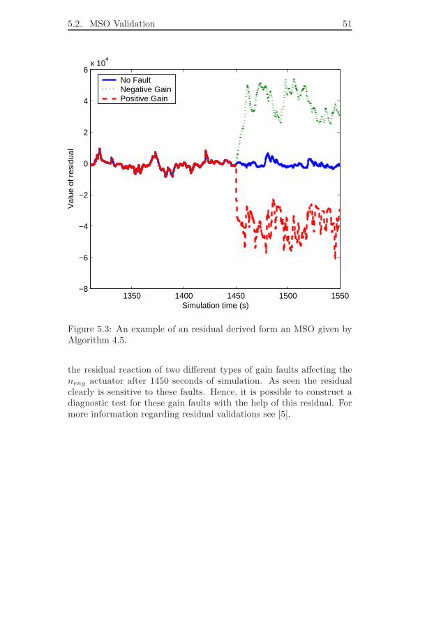
5.2. MSO Validation 51
1350 1400 1450 1500 1550−8
−6
−4
−2
0
2
4
6x 10
4
Simulation time (s)
Val
ue o
f res
idua
lNo FaultNegative GainPositive Gain
Figure 5.3: An example of an residual derived form an MSO given byAlgorithm 4.5.
the residual reaction of two different types of gain faults affecting theneng actuator after 1450 seconds of simulation. As seen the residualclearly is sensitive to these faults. Hence, it is possible to construct adiagnostic test for these gain faults with the help of this residual. Formore information regarding residual validations see [5].

Chapter 6
Conclusions and Future
Work
In this chapter the results and conclusions are presented in Section 6.1.Then in Section 6.2 a possible extension to the work in this thesis isproposed.
6.1 Conclusions
Today’s society depends on complex and technically advanced mechan-ical systems. To design diagnostic systems for these systems are a timedemanding and complex task. Hence, it is preferable, if as much ofthe construction process as possible can be automated. This thesis haspresented a number of algorithms and methods in order to make thispossible.
Since the models considered in this thesis were implemented in Simulink,there was a need to develop an algorithm that could transform thesemodels into analytical equations. By treating Simulink blocks as equa-tions and lines as variables, a transformation into analytical equationswas possible, see Section 3.1.2. Section 3.3 introduced a way in whichfault models can be included graphically directly into a Simulink model,in order to increase the diagnostic performance of the resulting diag-nostic system. The main objective in this thesis was to find the partsof a model that can be used to construct diagnostic tests. It provedto be an almost impossible task to perform this analytically, on themodels considered in this thesis. Hence, the analytical models weretransferred into a less complex mathematical format called structuralmodels. Structural models allow a complex analytical model to bepresented as a simple matrix, which decreases the execution times on
52

6.2. Future Work 53
certain calculations significantly. By using graph theory, it has beenshown that the task of finding all parts of a model that can be used inthe construction of a diagnostic system can be reduced to finding allminimal structurally overdetermined (MSO) sets in these models. Analgorithm for finding all MSO sets in a structural model has been devel-oped prior to this thesis. However, in test runs this algorithm showedto be extremely computationally ineffective and even unable to pro-duce results for the models considered in this work. In Chapter 4 newalgorithms for finding these MSO sets are presented. Especially thestructural simplification Algorithm 4.3 and the improved MSO findingAlgorithm 4.5, proved to be important in order to perform the extrac-tion of the MSO sets efficiently. Test runs verified the efficiency of thesealgorithms. It took less than a minute to extract all MSO sets fromthe models considered in this thesis. In Section 4.5 the correctness ofthe new MSO algorithms were proved mathematically. The concept ofoverdeterminedness introduced in Chapter 2 proved to be essential fordeveloping theory concerning the correctness of the algorithms.
All algorithms in this thesis have during this work been implementedand tested on various truck engine models provided by Scania CV AB.The conclusion drawn from these tests is that finding all parts of amodel that can be used to construct diagnostic test, can be preformedin an efficient and automated way. In Chapter 5 it was shown thatthese MSO sets could be used to form residuals. Hence, this thesis hasconstructed a foundation toward a completely automated constructionprocess of model based diagnostic systems. In theory this means thata diagnostic system can be constructed from, for example an enginemodel, completely automatic and in a fraction of the time it wouldtake to do it manually.
6.2 Future Work
The structural algorithms in this thesis only treat DLSMs (see Section2.4.1), i.e. structural models where a variable and its derivatives aretreated as the same signal. However, in some cases simpler residualscan be obtained form MSO sets of DSSMs, as the next example willshow. Consider the following model
e1 : y = x1
e2 : x1 = x1
e3 : x1 = u(6.1)
where y and u can be considered to be known. By using a DLSM thismodel can be transformed into the following structure

54 Chapter 6. Conclusions and Future Work
equation unknown knownx1 u y
e1 x xe2 xe3 x x
where three MSO sets can be obtained as e1, e2, e1, e3, e2, e3. Byusing these MSO sets three residuals can be constructed as r1 = y − y,r2 = u − y and r3 = u − u. However, by using a DSSM instead, (6.1)can be transformed into the following structure
equation unknown knownx1 x1 u y
e1 x xe2 x xe3 x x
with only one MSO e1, e2, e3. By using this MSO it is now possibleto create a residual like r4 = y − u, and hence completely avoid anyderivatives. For some model types, using DSSMs instead of DLSMs istherefor an advantage. This causes, on the other hand, another prob-lem. By using the three residuals derived from the DLSM above it ispossible to separate faults in the signals y and u from each other. Thisis not the case for the residual r4, which is sensitive to both faults. Asolution to this problem is to include derivatives of certain equationsinto the structural model. However, when doing this new problemsarise. Firstly the structural model will become significantly larger andsecondly, it may be uncertain how many derivatives that must be ex-tracted from a specific equation.
Seemingly, there are pros and cons with both structural model typesand today it is therefore impossible to say that one structure is betterthen the other. In order to investigate this further, algorithms for han-dling DSSMs could be seen as an extension to the work presented inthis thesis.

References
[1] Denley T. & Haggkvist R. Asratian A. Bipartite Graphs andtheir Applications. Cambridge University Press, Cambridge, UnitedKingdom, 1998.
[2] Lunze J. & Staroswiecki M. Blanke M., Kinnaert M. Diagnosis andFault-Tolerant Control. Linkoping, Sweden, 2004.
[3] Ericson C. Mean value modelling of a poppet valve egr-system.Master’s thesis LiTH-ISY-EX-3542-2004, Department of ElectricalEngineering, Linkopings Universitet, Linkoping, Sweden, May 2004.
[4] Nyberg M. & Frisk E. Model Based Diagnosis of TechnicalProcesses. Linkoping, Sweden, 2004.
[5] Krigsman K. &. Nilsson J. Code generation for efficient real-time execution of diagnostic residual generators. Master’s thesisIMIT/LECS-2004-66, The Department of Microelectronics and In-formation Technology, Royal Institute of Technology, Stockholm,Sweden, December 2004.
[6] Cassar J. & Staroswiecki M. A structural approach for the designof failure detection and identification systems. In IFAC Control ofIndustrial Systems, Belford, France, 1997.
[7] Krysander M. Design and analysis of diagnostic systems utilizingstructural methods, September 2003.
[8] Dulmage A. & Mendelsohn N.S. Coverings of bipartite graphs.Canadian Journal of Mathematics, (10):517–534, January 1958.
[9] Isermann R. & Balle P. Trends in the application of model-basedfault detection and diagnosis of technical processes. Control Eng.Practice, 5(5):709–719, March 1997.
55

56
Copyright
Svenska
Detta dokument halls tillgangligt pa Internet - eller dess framtida ersattare- under en langre tid fran publiceringsdatum under forutsattning attinga extra-ordinara omstandigheter uppstar.Tillgang till dokumentet innebar tillstand for var och en att lasa, lad-da ner, skriva ut enstaka kopior for enskilt bruk och att anvanda detoforandrat for ickekommersiell forskning och for undervisning. Overforingav upphovsratten vid en senare tidpunkt kan inte upphava detta tillstand.All annan anvandning av dokumentet kraver upphovsmannens medgi-vande. For att garantera aktheten, sakerheten och tillgangligheten finnsdet losningar av teknisk och administrativ art.Upphovsmannens ideella ratt innefattar ratt att bli namnd som up-phovsman i den omfattning som god sed kraver vid anvandning avdokumentet pa ovan beskrivna satt samt skydd mot att dokumentetandras eller presenteras i sadan form eller i sadant sammanhang somar krankande for upphovsmannens litterara eller konstnarliga anseendeeller egenart.For ytterligare information om Linkoping University Electronic Pressse forlagets hemsida: http://www.ep.liu.se/
English
The publishers will keep this document online on the Internet - or itspossible replacement - for a considerable time from the date of publi-cation barring exceptional circumstances.The online availability of the document implies a permanent permis-sion for anyone to read, to download, to print out single copies for yourown use and to use it unchanged for any non-commercial research andeducational purpose. Subsequent transfers of copyright cannot revokethis permission. All other uses of the document are conditional on theconsent of the copyright owner. The publisher has taken technical andadministrative measures to assure authenticity, security and accessibil-ity.According to intellectual property law the author has the right to bementioned when his/her work is accessed as described above and to beprotected against infringement.For additional information about the Linkoping University ElectronicPress and its procedures for publication and for assurance of documentintegrity, please refer to its WWW home page: http://www.ep.liu.se/

c© Lars ErikssonLinkoping, 10th January 2005