structural design using cellular automata - digital library and

Structural Design Using Cellular Automata

by

Douglas J. Slotta

Thesis submitted to the Faculty of the

Virginia Polytechnic Institute and State University

in partial fulfillment of the requirements for the degree of

MASTER OF SCIENCE

in

Computer Science and Applications

APPROVED:

Layne T. Watson

Zafer Gurdal Calvin J. Ribbens

May, 2001

Blacksburg, Virginia

Keywords: cellular automata, massively parallel processing, structural analysis.

Copyright 2001, Douglas J. Slotta

Structural Design Using Cellular Automata

Douglas J. Slotta

(ABSTRACT)

Traditional parallel methods for structural design do not scale well. This thesis discusses

the application of massively scalable cellular automata (CA) techniques to structural design.

There are two sets of CA rules, one used to propagate stresses and strains, and one to

perform design analysis. These rules can be applied serially, periodically, or concurrently,

and Jacobi or Gauss-Seidel style updating can be done. These options are compared with

respect to convergence, speed, and stability.

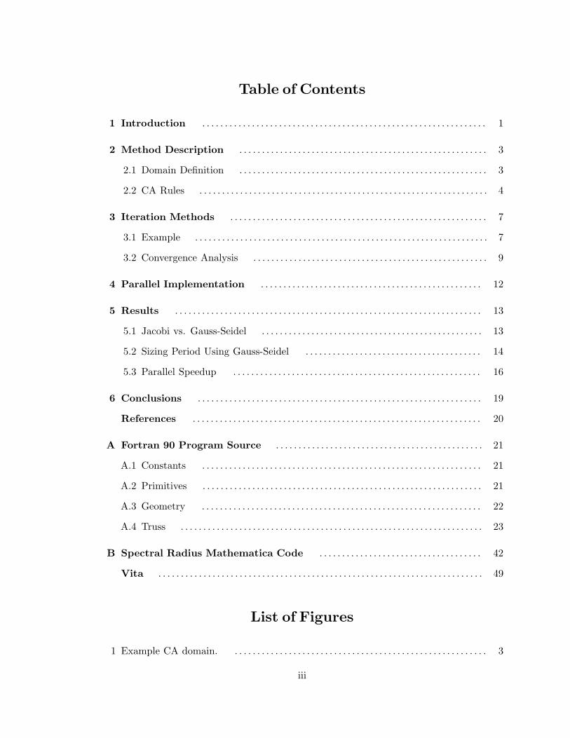
Table of Contents

1 Introduction . . . . . . . . . . . . . . . . . . . . . . . . . . . . . . . . . . . . . . . . . . . . . . . . . . . . . . . . . . . . . . . 1

2 Method Description . . . . . . . . . . . . . . . . . . . . . . . . . . . . . . . . . . . . . . . . . . . . . . . . . . . . . . . 3

2.1 Domain Definition . . . . . . . . . . . . . . . . . . . . . . . . . . . . . . . . . . . . . . . . . . . . . . . . . . . . . . . 3

2.2 CA Rules . . . . . . . . . . . . . . . . . . . . . . . . . . . . . . . . . . . . . . . . . . . . . . . . . . . . . . . . . . . . . . . . 4

3 Iteration Methods . . . . . . . . . . . . . . . . . . . . . . . . . . . . . . . . . . . . . . . . . . . . . . . . . . . . . . . . . 7

3.1 Example . . . . . . . . . . . . . . . . . . . . . . . . . . . . . . . . . . . . . . . . . . . . . . . . . . . . . . . . . . . . . . . . . 7

3.2 Convergence Analysis . . . . . . . . . . . . . . . . . . . . . . . . . . . . . . . . . . . . . . . . . . . . . . . . . . . . 9

4 Parallel Implementation . . . . . . . . . . . . . . . . . . . . . . . . . . . . . . . . . . . . . . . . . . . . . . . . . 12

5 Results . . . . . . . . . . . . . . . . . . . . . . . . . . . . . . . . . . . . . . . . . . . . . . . . . . . . . . . . . . . . . . . . . . . . 13

5.1 Jacobi vs. Gauss-Seidel . . . . . . . . . . . . . . . . . . . . . . . . . . . . . . . . . . . . . . . . . . . . . . . . . 13

5.2 Sizing Period Using Gauss-Seidel . . . . . . . . . . . . . . . . . . . . . . . . . . . . . . . . . . . . . . . 14

5.3 Parallel Speedup . . . . . . . . . . . . . . . . . . . . . . . . . . . . . . . . . . . . . . . . . . . . . . . . . . . . . . . 16

6 Conclusions . . . . . . . . . . . . . . . . . . . . . . . . . . . . . . . . . . . . . . . . . . . . . . . . . . . . . . . . . . . . . . . 19

References . . . . . . . . . . . . . . . . . . . . . . . . . . . . . . . . . . . . . . . . . . . . . . . . . . . . . . . . . . . . . . . . 20

A Fortran 90 Program Source . . . . . . . . . . . . . . . . . . . . . . . . . . . . . . . . . . . . . . . . . . . . . . 21

A.1 Constants . . . . . . . . . . . . . . . . . . . . . . . . . . . . . . . . . . . . . . . . . . . . . . . . . . . . . . . . . . . . . . 21

A.2 Primitives . . . . . . . . . . . . . . . . . . . . . . . . . . . . . . . . . . . . . . . . . . . . . . . . . . . . . . . . . . . . . . 21

A.3 Geometry . . . . . . . . . . . . . . . . . . . . . . . . . . . . . . . . . . . . . . . . . . . . . . . . . . . . . . . . . . . . . . 22

A.4 Truss . . . . . . . . . . . . . . . . . . . . . . . . . . . . . . . . . . . . . . . . . . . . . . . . . . . . . . . . . . . . . . . . . . . 23

B Spectral Radius Mathematica Code . . . . . . . . . . . . . . . . . . . . . . . . . . . . . . . . . . . . 42

Vita . . . . . . . . . . . . . . . . . . . . . . . . . . . . . . . . . . . . . . . . . . . . . . . . . . . . . . . . . . . . . . . . . . . . . . . . 49

List of Figures

1 Example CA domain. . . . . . . . . . . . . . . . . . . . . . . . . . . . . . . . . . . . . . . . . . . . . . . . . . . . . . . . . 3

iii

2 Example non-rectangular CA domain. . . . . . . . . . . . . . . . . . . . . . . . . . . . . . . . . . . . . . . . . 4

3 Simple bridge truss, before and after running CA. . . . . . . . . . . . . . . . . . . . . . . . . . . . . 7

4 Bridge truss with smaller cells, converged. . . . . . . . . . . . . . . . . . . . . . . . . . . . . . . . . . . . . 7

5 Jacobi vs. Gauss-Seidel iteration methods. . . . . . . . . . . . . . . . . . . . . . . . . . . . . . . . . . . 13

6 Jacobi vs. Gauss-Seidel for analysis only. . . . . . . . . . . . . . . . . . . . . . . . . . . . . . . . . . . . . 13

7 Undamped sizing with Gauss-Seidel iteration. . . . . . . . . . . . . . . . . . . . . . . . . . . . . . . . 15

8 Damped sizing with Gauss-Seidel iteration. . . . . . . . . . . . . . . . . . . . . . . . . . . . . . . . . . . 15

9 Timings on an Origin 2000. . . . . . . . . . . . . . . . . . . . . . . . . . . . . . . . . . . . . . . . . . . . . . . . . . 16

10 Timings on a Beowulf cluster. . . . . . . . . . . . . . . . . . . . . . . . . . . . . . . . . . . . . . . . . . . . . . . . 16

List of Tables

1 Spectral radius . . . . . . . . . . . . . . . . . . . . . . . . . . . . . . . . . . . . . . . . . . . . . . . . . . . . . . . . . . . . . . 10

iv

1. Introduction

The traditional method of doing structural analysis and design uses finite element based

numerical analysis programs. While this approach works well for many problems, it does

not parallelize efficiently on massively parallel processors (MPPs), thus limiting the size and

complexity of the designs that can be analyzed and optimized. A new approach is needed

that works well on MPPs. This method need not be faster than those currently used for

serial machines on problems that do not exhaust the machines’ resources; rather it needs

to allow each processor of a MPP enough useful work such that large problems beyond the

resources of serial or moderately parallel machines can be solved in acceptable times.

Cellular automata (CA) were used at least as early as 1946 by Weiner and Rosenblunth

[13] to describe the operation of heart muscle, even though their use was not computationally

feasible at the time. CA tiles a problem domain into cells of equal size. Each cell has

the same set of simple rules that dictate how it behaves and interacts with its neighboring

cells. The principle is that an overall global behavior can be computed by a group of cells

that only know local conditions [14]. If each cell only needs to know local conditions, then

this minimizes the communication requirements and therefore the problem scales well on a

MPP. A CA is the archetypical algorithm for the SIMD parallel architecture [1].

A cellular automaton is a discrete dynamical system [14]. It is discrete in the sense

that space and time are discrete. Each cell is a fixed point in a regular lattice. The state of

each cell is updated at discrete time steps, based upon conditions in previous time steps.

All of the cells are updated every time step, thus the state of the entire lattice is updated

every time step.

In general, CA are used to simulate the dynamic behavior of physical systems, and

have been used successfully to represent a variety of phenomena such as diffusion of gaseous

systems, solidification and crystal growth in solids, and hydrodynamic flow and turbulence

[12]. CA has also recently been used in conjunction with genetic algorithms to derive the

rules required at each cell to perform structural analysis [6]. CA rules have recently been

devised for the simultaneous analysis and design of simple two-dimensional structures [4,

1

11]. That work is the basis for this thesis. In the case of structural design, the intention

is to describe a static equilibrium of a structure under a system of forces acting on it.

In this sense, time is not being simulated, rather each step of the automaton is used to

propagate (local) stresses and strains through a structure to allow it to reach equilibrium

state while simultaneously determining the shape and/or dimensions of the cells associated

with this equilibrium state. This is continued until the entire process converges (ideally)

to a global state where there is no significant change in the structure for every subsequent

iteration, corresponding to a static equilibrium state. Note that analysis and design are

done simultaneously and locally by each cell.

This thesis will begin by describing the CA used to do structural design on ground

trusses in Chapter 2 and give an example. Chapter 3 will discuss the merits of two different

iteration methods. Chapter 4 will explain how the CA is parallelized, and finally Chapter

5 will discuss some preliminary results.

2

2. Method Description

The basic elements of the structural design CA consist of the division of the problem

into cells and the three types of rules that can operate on those cells. Each of the rules

operates on the cells using the information in a Moore neighborhood, which consists of the

surrounding nine cells. The first set of rules are used to do analysis only, determining the

stresses and strains in each cell. The second set of rules does the design work, changing

the areas of the connecting beams to withstand the stresses. The final set of rules performs

simultaneous analysis and design.

2.1 Domain Definition

Each cell of this CA is an eight-beam truss where each beam starts at the center of

the cell and connects to its opposite member in an adjacent cell as illustrated in Figure 1.

Figure 1. Example CA domain with a single cell denoted by the dashed line.

3

This type of structure is known as a ground truss. Those cells which fall on the border

of the rectangular domain are not partial cells requiring special rules, but are complete

cells with the area of the beams that fall outside the computational domain set to zero. In

addition, they are connected to an invisible set of surrounding cells that are turned off and

that also have all of their beam areas set to zero. Cells that are turned off are not part

of the computation, being used only to make the rules for the border and non-border cells

consistent, since the stress analysis rules require the displacements of all eight surrounding

cells.

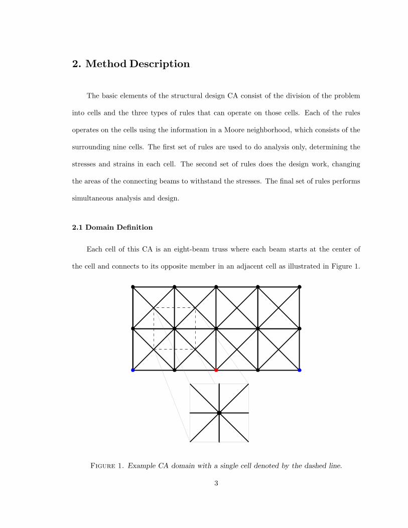
The actual border of the computational domain of the CA need not be rectangular.

Any shape can be defined for the truss by turning off any cells that are not within the

computational domain, as illustrated in Figure 1. A simple method to define a shape for

the truss is to define an enclosing polygon, and then turn off every cell that does not fall

within the polygon. A more sophisticated method could be used to allow for holes, circular

regions, or other, nonstraight boundaries.

The “edge crossings” algorithm [8] to determine those points within the polygon can

be used; it is simple and parallelizes well. From each point, a ray is cast, usually in the

horizontal direction, and the number of edges that it crosses are counted. If there are an

odd number of edges, then the point is within the polygon. If there are an even number of

edges, then the point is outside the polygon. Special care must be taken for those points

that are on the edge, or where the ray happens to intersect a vertex. A Fortran 90 module

implementing this is included in Appendix A.3.

As seen in Figure 2, only those polygons that are composed of lines with slopes 0,

1, −1, or ∞ will be represented exactly. This is the same aliasing problem that bitmaps

face. A better resolution can be obtained by decreasing the cell size in the domain, thereby

increasing the number of cells that form the shape. This is the same as smoothing the

outline of a bitmap by increasing the number of pixels that form the bitmap. The amount

by which the original cells have been subdivided to increase the resolution is known as the

cell density factor (CDF).

4

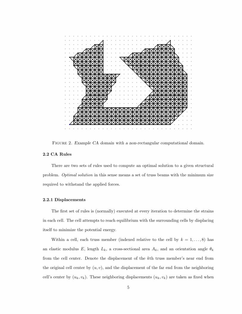
Figure 2. Example CA domain with a non-rectangular computational domain.

2.2 CA Rules

There are two sets of rules used to compute an optimal solution to a given structural

problem. Optimal solution in this sense means a set of truss beams with the minimum size

required to withstand the applied forces.

2.2.1 Displacements

The first set of rules is (normally) executed at every iteration to determine the strains

in each cell. The cell attempts to reach equilibrium with the surrounding cells by displacing

itself to minimize the potential energy.

Within a cell, each truss member (indexed relative to the cell by k = 1, . . . , 8) has

an elastic modulus E, length Lk, a cross-sectional area Ak, and an orientation angle θk

from the cell center. Denote the displacement of the kth truss member’s near end from

the original cell center by (u, v), and the displacement of the far end from the neighboring

cell’s center by (uk, vk). These neighboring displacements (uk, vk) are taken as fixed when

5

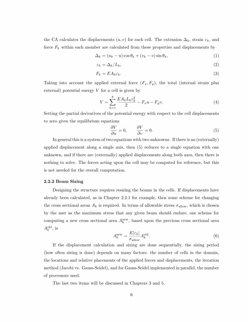
the CA calculates the displacements (u, v) for each cell. The extension ∆k, strain εk, and

force Fk within each member are calculated from these properties and displacements by

∆k = (uk − u) cos θk + (vk − v) sin θk, (1)

εk = ∆k/Lk, (2)

Fk = EAkεk. (3)

Taking into account the applied external force (Fx, Fy), the total (internal strain plus

external) potential energy V for a cell is given by

V =8

∑

k=1

EAkLkε2k

2− Fxu− Fyv. (4)

Setting the partial derivatives of the potential energy with respect to the cell displacements

to zero gives the equilibrium equations

∂V

∂u= 0,

∂V

∂v= 0. (5)

In general this is a system of two equations with two unknowns. If there is an (externally)

applied displacement along a single axis, then (5) reduces to a single equation with one

unknown, and if there are (externally) applied displacements along both axes, then there is

nothing to solve. The forces acting upon the cell may be computed for reference, but this

is not needed for the overall computation.

2.2.2 Beam Sizing

Designing the structure requires resizing the beams in the cells. If displacements have

already been calculated, as in Chapter 2.2.1 for example, then some scheme for changing

the cross sectional areas Ak is required. In terms of allowable stress σallow, which is chosen

by the user as the maximum stress that any given beam should endure, one scheme for

computing a new cross sectional area Anewk , based upon the previous cross sectional area

Aoldk , is

Anewk =

E|εk|

σallowAold

k . (6)

If the displacement calculation and sizing are done sequentially, the sizing period

(how often sizing is done) depends on many factors: the number of cells in the domain,

the locations and relative placements of the applied forces and displacements, the iteration

method (Jacobi vs. Gauss-Seidel), and for Gauss-Seidel implemented in parallel, the number

of processors used.

The last two items will be discussed in Chapters 3 and 5.

6

3. Iteration Methods

Each cell depends on the displacements of the surrounding cells to calculate its own

displacement, thereby propagating the stresses and strains. This is repeated until the

structure no longer changes appreciatively, at which point it is said to have converged.

The convergence criterion for the displacement of a cell is defined by the condition that

the current change in displacement is a small fraction or percentage (usually 10−6) of the

maximum displacement within the structure. The sizing convergence criterion is analogous.

For an entire structure to be considered converged with respect to displacement or sizing,

every cell within that structure must meet the convergence criterion for that update rule.

One method of implementing a CA is to keep two copies of the array of cells, one to

represent time t, and the other to represent time t + 1. The values for the cells at t + 1

are calculated from the cells at t. At the end of this iteration, the labels of the arrays are

swapped, and the process is repeated. This is a Jacobi iteration, where all of the new values

are calculated from the old values.

For any process that converges, using a Jacobi iteration method can be inefficient [1].

By using a Gauss-Seidel iteration method, where new values are calculated using updated

values, the process should converge using fewer iterations. This means that only one copy

of the array is kept. When a new displacement is calculated for one cell, then the next

adjacent cell will use that updated value when calculating its own displacement. Note that

this does not apply to the sizing rules since, as defined, their application is independent of

the information in the surrounding cells.

3.1 Example

Consider the problem of a simple bridge truss. The first image in Figure 3 shows a

CA with six cells. The bottom two corner cells have an applied displacement of (0,0) so

they are fixed in place. The bottom middle cell has an applied force of 100kN downward.

The width of the bridge is 50 meters and the height is 25 meters. The bars are composed

7

Figure 3. Simple bridge truss, before and after running CA.

Figure 4. Bridge truss with same dimensions, smaller cells, converged.

of medium steel (E = 200GPa and σallow = 250MPa). Each beam has an initial area of

0.0175m2.

Running the CA on the bridge problem using the Gauss-Seidel iteration method for

displacements and applying the sizing rules every sixth iteration until it converges at iteration

253, the result shown in the second image of Figure 3 is obtained. Since the bridge is 50m

across and the steel beams are no more than a few cm thick, the areas in this view are

exaggerated by a factor of 3000 to show the differences in the beam sizes.

8

The bridge in Figure 3 is only composed of eleven trusses, and the solution could easily

have been computed by hand. But if each beam is required to be less than 25m long, the

complexity of the problem rises. Figure 4 shows a problem of the exact same dimensions,

where each cell is 40 times smaller than previously. Each horizontal and vertical beam is

0.625m long, rather than 25m.

3.2 Convergence Analysis

To analyze the efficacy of the iteration method used, it is useful to transform the CA

into an equivalent system of linear equations. Recall from Chapter 2.2.1 that each cell is

computing its position (u, v) based upon the position of the surrounding cells. If each cell

were assigned unique variables for its position, such that cell 1 has u1 and v1, cell 2 has

u2 and v2, and so forth, then the equations for each cell can be expressed in terms of the

variables for the surrounding cells. For a CA structure composed of 6 cells, this will form

a linear system of 12 equations and 12 unknowns.

This standard system of linear equations,

Ax = b, (7)

can be solved by the Jacobi and Gauss-Seidel fixed-point iteration methods or block versions

thereof, which are the exact mathematical formulations of the local cell calculations. For

the Jacobi, A is split into its strictly 2× 2 block lower triangular (L), 2× 2 block diagonal

(D), and strictly 2× 2 block upper triangular (U) parts,

A = L+D+U. (8)

The system is then rewritten as a fixed point iteration where the next iterate x(n+1) is

computed from the previous iterate x(n) via

x(n+1) = Bx(n) +C, (9)

where

B = −D−1(L+U), C = D−1b. (10)

9

CDF n Jacobi Gauss-Seidel

1 8 0.794104 0.611503

2 26 0.949748 0.8982

3 52 0.979368 0.959006

4 86 0.989496 0.978893

5 128 0.993801 0.987605

6 178 0.995959 0.991925

7 236 0.997181 0.994365

8 302 0.997933 0.995865

9 376 0.998426 0.996853

10 458 0.998765 0.997532

Table 1. Spectral radius of the bridge truss for various CDFs.

Note that Ax = b if and only if x = Bx+C, assuming D−1 exists. For Gauss-Seidel

the iteration x(n+1) = Bx(n) +C has

B = −(D+ L)−1U, C = (D+ L)−1b, (11)

assuming (D+ L)−1 exists.

The fixed point iteration (9) converges for any starting point x(0) if and only if all of

the eigenvalues of B are less than one in absolute value [7]. The maximum absolute value

of the eigenvalues for a matrix is called the spectral radius. The spectral radius for the

bridge structure at various CDFs is shown in Table 1. The n column denotes the number

of equations and number of unknown variables being solved for a given CDF.

This table shows that the Jacobi or Gauss-Seidel CA iteration for analysis does converge,

but extremely slowly. For larger CDFs, the improvement of Gauss-Seidel over Jacobi is

marginal. Even with massive parallelism, any competitive advantage of CA (over solving

the linear system with standard iterative numerical methods) must come by combining

analysis with sizing.

10

Aitken’s δ2 method [7] was also explored. This method uses the (scalar) values of three

successive iterations to extrapolate a value (hopefully) closer to the fixed-point value. This

method requires that (for scalar values xn)

∆xn+1

∆xn

≈∆xn

∆xn−1≈

∆xn−1

∆xn−2≈ A, (12)

where |A| < 1. However, this requirement was not met by the components x(n)i of the vector

iteration (9), and therefore Aitken’s δ2 acceleration method was not applicable.

11

4. Parallel Implementation

The code for this CA was implemented in Fortran 90 using the Message Passing Interface

(MPI) library as its parallel communication mechanism. It has been tested on both an

Origin 2000 with 64 processors and a Beowulf cluster with 32 processors.

A parallel decomposition was performed by dividing the computational domain into

vertical strips and assigning each strip of contiguous cells to a single processor. Each strip

has an additional column of border cells on either side that are turned off. These border

cells represent the connected cells located on the adjacent processors. At every iteration, a

processor computes the updated values for its cells, and then exchanges its left and right

columns with its neighbors. These updated values are stored in the border cells and used

for the next iteration. Therefore the natural communication topology is a ring topology,

which easily maps into most other communication topologies.

Stripped partitioning works well for a rectangular shaped domain because it provides a

good balance of computation to communication. It does have some limitations, for example,

given a domain size of N rows ×M cols, there can be at most M processors; if M < N then

the lattice can be trivially rotated. For those problems with an irregular shape, there will

not be the same balance of computation to communication at every processor. For these

cases, a more efficient partitioning method (e.g., graph-based partitioning) should be used.

When implementing the Gauss-Seidel iterationmethod in parallel, no attempt is made to

keep the order in which the cells are updated the same as in the non-parallel implementation.

Instead, each processor iterates over its collection of cells as if it were the sole processor

operating on the domain, where the domain consists of its assigned cells, plus a group of

surrounding “dead” cells that are not computed. The “dead” cells are used to contain the

updated values from the adjacent processors that are sent at the end of every iteration.

Since the Gauss-Seidel iteration is contained solely within each processor, the rate of

convergence differs depending upon the number of processors used. This has an effect upon

the stability of the calculation as will be seen in Chapter 5.1. On the other hand, the

programming task is much easier since, except for the initial setup and the communication

at the end of every iteration, the program is exactly the same as the Gauss-Seidel iteration

for a single processor.

12

5. Results

5.1 Jacobi vs. Gauss-Seidel

When comparing the performance of Jacobi and Gauss-Seidel iteration methods it is

useful to look at the number of iterations it takes the displacements (without sizing) to

converge using a single processor. Figure 5 compares the number of iterations to the vertical

displacement of the mid-span of the bridge truss with a CDF (cell density factor) of 16. The

mid-span will have the largest displacement for any correct solution to the problem because

it has the only externally applied force. Figure 5 shows that it takes 12,808 iterations to

converge with the Jacobi method and only 6,723 iterations using the Gauss-Seidel.

-0.025

-0.02

-0.015

-0.01

-0.005

0

0 2500 5000 7500 10000 12500

Iterations

-0.01

-0.009

-0.008

-0.007

-0.006

-0.005

-0.004

0 1 2 3 4 5 6 7 8 9 10 11 12 13 14 15 16 17 18 19 20

Ver

ticle

Dis

plac

emen

ts a

t Mid

-Spa

n

Gauss-Seidel AnalysisJacobi AnalysisGauss-Seidel DesignJacobi Design

Figure 5. Comparison between Jacobi and Gauss-Seidel iteration

methods on the bridge structure with a CDF of 16.

The speed of convergence for a structural analysis CA is affected by more than just the

iteration method if sizing rules are used as well. Figure 5 also has an expanded view of the

first 20 iterations that includes sizing rules applied every four iterations. Note that when

using the Jacobi method with sizing, the maximum displacement diverges away quickly

13

0 5 10 15 20 25 300

2000

4000

6000

8000

10000

12000

14000

16000

CDF = 16

Jacobi Iterations

Gauss-Seidel

Iter

atio

ns

Number of Processors

Figure 6. Comparison between Jacobi and Gauss-Seidel iteration methods for

analysis only on the bridge structure with a cell density factor of 16.

from the maximum displacement using analysis only. In fact, for this sizing period, the CA

is non-convergent. For the Gauss-Seidel method with sizing applied every n iterations, the

CA is usually more stable and converges quicker.

As mentioned previously, when using a Gauss-Seidel iteration, the rate of convergence

differs depending upon the number of processors used. As shown in Figure 6 for analysis

with no sizing, the number of iterations needed to converge increases as the number of

processors increases. As the number of processors increases, the smaller the number of cells

each processor contains, and therefore the less area each stress and strain can propagate each

iteration. Intuitively, this continues until each processor has exactly one cell and (parallel)

Gauss-Seidel iteration is exactly the same as Jacobi.

5.2 Sizing Period Using Gauss-Seidel

As seen in the previous section, the choice of how often to apply sizing rules is very

important to the speed and the stability of the CA. Since the design equations allow the

areas of the bars to adjust fully to the surrounding stresses and strains, it is possible that

14

0 10 20 30 40 50Sizing Period

0

3

6

9

12

15

CDF

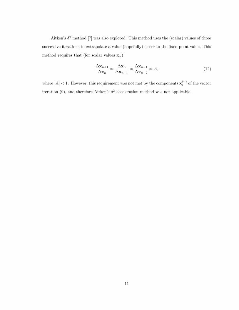
Figure 7. Convergence data using undamped sizing with Gauss-Seidel iteration.

0 10 20 30 40 50Sizing Period

0

3

6

9

12

15

CDF

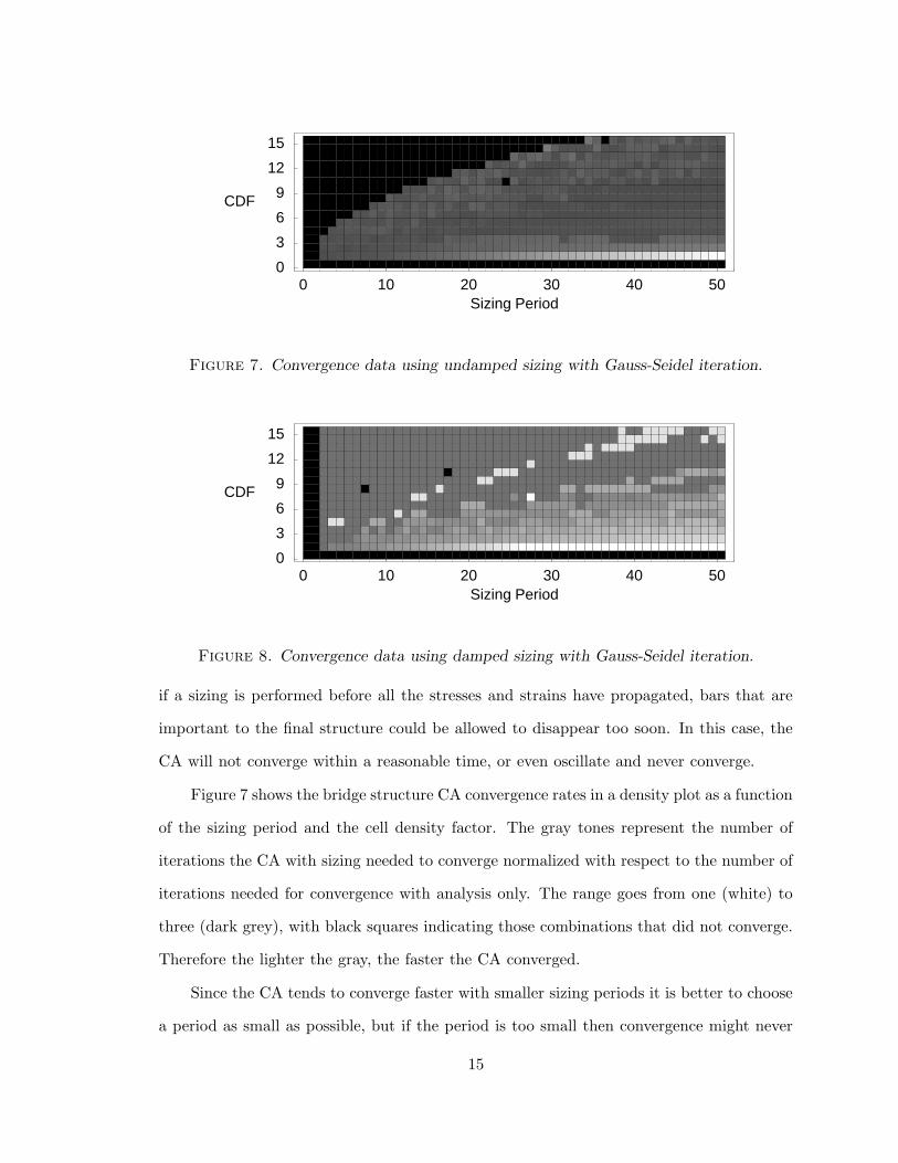
Figure 8. Convergence data using damped sizing with Gauss-Seidel iteration.

if a sizing is performed before all the stresses and strains have propagated, bars that are

important to the final structure could be allowed to disappear too soon. In this case, the

CA will not converge within a reasonable time, or even oscillate and never converge.

Figure 7 shows the bridge structure CA convergence rates in a density plot as a function

of the sizing period and the cell density factor. The gray tones represent the number of

iterations the CA with sizing needed to converge normalized with respect to the number of

iterations needed for convergence with analysis only. The range goes from one (white) to

three (dark grey), with black squares indicating those combinations that did not converge.

Therefore the lighter the gray, the faster the CA converged.

Since the CA tends to converge faster with smaller sizing periods it is better to choose

a period as small as possible, but if the period is too small then convergence might never

15

be achieved. To allow smaller sizing periods to be chosen, damping (in terms of the rate in

which the cross-sectional areas can change) was applied to the design equations. Damping

the sizing function limits the area to be within a certain percentage of the current value

of the bar area. Figure 8 shows the results for the same problem as in Figure 7 with 10%

damping applied.

In this case, farmore combinations of CDFs and sizing periods converged than previously,

especially when using smaller sizing periods. However, more iterations were needed for each

computation to converge than for sizing without damping. Thus there is a tradeoff between

speed of convergence and robustness of the code.

5.3 Parallel Speedup

Execution time for the Fortran 90 code was measured for the Gauss-Seidel version of

the code since it seemed to be the most stable version. Timing runs were done using a fixed

number of iterations that are below the number of iterations required for full convergence.

This was to eliminate the vagaries of convergence using Gauss-Seidel on different numbers

of processors. Parallel overhead was measured by taking a time stamp at the beginning

and end of every communication between processors at a single processor. The cumulative

time difference is the parallel overhead needed to pack the information, send it to adjacent

processors, wait for the updates from the other processors, and then finally unpack the

information.

The communication is using blocking MPI calls to aid in measurement, therefore the

computation time is the overall time minus the parallel overhead. The design easily allows

for a more efficient implementation overlapping the computation and communication by

using non-blocking MPI calls.

Figure 9 shows the timing results for an Origin 2000 using shared memory for the

communication channels. The data shown in Figure 9 is the average of 5 runs, and the

standard deviations ranged between 0.11 and 1.19. In this case, communication overhead

does not begin to dominate until about 64 processors are used.

Figure 10 shows the timing results for a Linux Beowulf system using 100Mbit Ethernet

between processor nodes. The data shown is the average of 5 runs, and the standard

deviations ranged between 0.29 and 0.46. Here the communication overhead dominates

from the beginning. The theoretical curve is the ideal speedup, serial time divided by the

number of processors.

16

0

20

40

60

80

100

120

140

8 16 24 32 40 48 56 64


Computation

Theoretical

Comm TimeSe

cond

s

Figure 9. Timings on an Origin 2000 machine for the bridge structure

with a CDF of 40 for 20,000 iterations.

17

0

10

20

30

40

50

60

70

80

90

8 16 24 32


Computation

Theoretical

Comm Time

Seco

nds

Figure 10. Timings on a Beowulf cluster for the bridge structure

with a CDF of 40 for 20,000 iterations.

18

6. Conclusions

Cellular automata techniques can be applied to structural design and allow efficient

use of MPPs. This potentially allows problems of far greater complexity to be solved in a

reasonable time. The technique is also easy to implement and is versatile in design of truss

topologies. Slow convergence and divergence of the CA is mathematically explained by the

spectral radius of the iteration matrix, for analysis only, but adding sizing makes the fixed

point iteration x(n+1) = F (x(n)) nonlinear. A topic for future work is the mathematical

analysis of the full nonlinear iteration. Future work could also include extending the method

to three dimensions and to creating more types of structures other than ground trusses.

19

References

[1] Bertsekas, D. and Tsitsiklis, J. (1989), Parallel and Distributed Computation,

Numerical Methods, Prentice Hall, Englewood Cliffs, NJ.

[2] Ca, J. and Thierauf, G. (1997), “Evolution strategies in engineering computation,”

Engineering Optimization, Vol. 29, pp. 177–199.

[3] Gaylord, R. and Nishidate, K. (1996), Modeling Nature: Cellular Automata

Simulations with Mathematica, Springer-Verlag, New York.

[4] Gurdal, Z. and Tatting, B. (2000), “Cellular automata for design of truss struc-

tures with linear and nonlinear response,” Proc. 41st AIAA/ASME/ASCE/AHS

Structures, Structural Dynamics, and Materials Conf., AIAA Paper 2000-1580,

Atlanta, GA.

[5] Hajela, P. and Kim, B. (1999), “GA based learning in cellular automata models

for structural analysis,” 3rd World Congress on Structural and Multidisciplinary

Optimization, Niagara Falls, NY.[6] Hajela, P. and Kim, B. (2000), “On the use of energy minimization for CA based

analysis in elasticity,” manuscript, in preparation.

[7] Issacson, E. and Keller, H. (1966), Analysis of Numerical Methods, Dover, New

York.

[8] O’Rourke, J. (1994), Computational Geometry in C, Cambridge University Press,

Cambridge, MA.

[9]Quinn, M. (1993), Parallel Computing, Theory and Practice, McGraw Hill, New York.

[10] Quinn, M. (1993), Designing Efficient Algorithms for Parallel Computers, McGraw

Hill, New York.

[11]Tatting, B. andGurdal, Z. (2000), “Cellular automata for design of two-dimensional

continuum structures,” Proc. 8th AIAA/NASA/ISSMO Symp. on Multidisci-

plinary Analysis and Optimization, AIAA Paper 2000-4832, Long Beach, CA.

[12] Toffoli, T. and Margolus, N. (1991), Cellular Automata Machines, MIT Press,

Cambridge, MA.

[13] Weiner, N. and Rosenblunth, A. (1946), “The mathematical formulation of the

problem of conduction of impulses in a network of connected excitable elements,

specifically in cardiac muscle,” Arch. Inst. Cardiol. Mexico, Vol. 16, pp. 205–265.

[14]Wolfram, S. (1994), Cellular Automata and Complexity: Collected Papers, Addison-

Wesley, Reading, MA.

20

Appendix A

The code for this CA was implemented in Fortran 90 using the Message Passing Interface

(MPI) library as its parallel communication mechanism. The code uses the non-standard

getarg routine, which is not in the Fortran 90 specification. The code has been successfully

compiled and run on an Origin 2000 using the SGI compiler, Linux using the Portland

Group compiler, Win32 using the Digital F90 compiler, and Digital Unix on a Dec Alpha

using the Digital F90 compilers.

A.1

!-----------------------------------------

! Constants and tuning parameters

!-----------------------------------------

module constants

implicit none

save

integer, parameter :: MAX_DIM = 10000

integer, parameter :: CMD_LEN = 250

double precision, parameter :: EPSILON = 1.0D-6

double precision, parameter :: SQRT2 = 1.414213562373095

double precision, parameter :: RF = 0.01

!Cell directions

integer, parameter :: SW = 1

integer, parameter :: SOUTH = 2

integer, parameter :: SE = 3

integer, parameter :: WEST = 4

integer, parameter :: EAST = 5

integer, parameter :: NW = 6

integer, parameter :: NORTH = 7

integer, parameter :: NE = 8

end module constants

A.2

!-----------------------------------------

! Contains data types and provides 64-bit reals on all platforms

!-----------------------------------------

module primitives

use geometry

implicit none

type modifier

character :: xType, yType

type(iPoint) :: location

type(rPoint) :: component

end type modifier

type cell

logical :: exists

logical :: conv

21

double precision :: u, v

double precision, dimension(8) :: area

type(modifier), pointer :: mod

end type cell

end module primitives

A.3

!-----------------------------------------

! Used to construct polygon and to determine cell existence.

!-----------------------------------------

module geometry

implicit none

type rPoint

double precision :: x, y

end type rPoint

type iPoint

integer :: x, y

end type iPoint

integer, private, save :: nVertices

type(iPoint), private, allocatable, dimension(:), save :: Polygon

contains

!-----------------------------------------

! Create space for the defined polygon

!-----------------------------------------

subroutine initPolygon(nVerts)

implicit none

integer, intent(in) :: nVerts

nVertices = 0

allocate(Polygon(0:(nVerts-1)))

end subroutine initPolygon

!-----------------------------------------

! Adds (integer) point (x,y) to the polygon

!-----------------------------------------

subroutine addPoint(x, y)

implicit none

integer, intent(in) :: x, y

Polygon(nVertices)%x = x

Polygon(nVertices)%y = y

nVertices = nVertices + 1

end subroutine addPoint

!-----------------------------------------

! Changes the size of the polygon by scaling all of the vertices

!-----------------------------------------

subroutine scalePolygon(scale)

implicit none

integer, intent(in) :: scale

Polygon(:)%x = Polygon(:)%x * scale

Polygon(:)%y = Polygon(:)%y * scale

end subroutine scalePolygon

!-----------------------------------------

! Purpose: Determines if a point is enclosed with the polygon.

!-----------------------------------------

logical function PointInPoly(q)

type(rPoint), intent(in) :: q

22

type(rPoint), allocatable, dimension(:) :: P

integer :: i, i1, rCross, lCross

double precision :: intersect

allocate(P(0:(nVertices-1)))

!Shift Polygon so that q is the origin

do i=0, (nVertices-1)

P(i)%x = Polygon(i)%x - q%x

P(i)%y = Polygon(i)%y - q%y

end do

rCross = 0

lCross = 0

!For each edge, e=(i-1, i) see if it crosses ray

do i=0, (nVertices-1)

!Check if q (0,0) is a vertex

if ((P(i)%x .eq. 0.0) .and. (P(i)%y .eq. 0.0)) then

PointInPoly = .true.

return

end if

i1 = MOD((i+nVertices-1), nVertices)

!Check if e straddles the x-axis

if (((P(i)%y > 0.0) .and. (P(i1)%y <= 0.0)) .or. &

((P(i1)%y > 0.0) .and. (P(i)%y <=0.0))) then

!if ((P(i)%y > 0.0) .ne. (P(i1)%y > 0.0)) then

!It does straddle, so compute intersection

intersect = (P(i)%x * P(i1)%y - P(i1)%x * P(i)%y ) / (P(i1)%y - P(i)%y)

if (intersect >= 0.0) then

rCross = rCross + 1

end if

end if

!Check if e straddles the x-axis when reversed

if (((P(i)%y < 0.0) .and. (P(i1)%y >= 0.0)) .or. &

((P(i1)%y < 0.0) .and. (P(i)%y >= 0.0))) then

!if ((P(i)%y < 0.0) .ne. (P(i1)%y < 0.0)) then

!It does straddle, so compute intersection

intersect = (P(i)%x * P(i1)%y - P(i1)%x * P(i)%y ) / (P(i1)%y - P(i)%y)

if (intersect <= 0.0) then

lCross = lCross + 1

end if

end if

end do

!q is an edge if left and right crossing are not the same parity

if (MOD(rCross, 2) .ne. MOD(lCross, 2)) then


return

end if

!q inside iff odd number of crossings

if (MOD(rCross, 2) == 1) then


else

PointInPoly = .false.

end if

deallocate( P )

end function PointInPoly

end module geometry

23

A.4

!-----------------------------------------

! Implementation of Cellular Automata

! technique for the solution of 2-D truss problems.

!-----------------------------------------

program Truss

use constants ! Various constants

use primitives

implicit none

include ’mpif.h’

! Define variables input by user

double precision :: initArea, minArea, eMod, dist, sigAllow

integer :: maxIterations, designRate, scale, nModifiers

character (len = CMD_LEN) :: datafile

logical :: printAll

! Computation control variables

logical :: gauss=.true.

logical :: linear=.true.

! Define additional variables used for solution

integer :: iLeft, iRight, iTop, iBottom, iteration

integer :: moveCount = 0, designCount = 0, oldMoveCount=0, newMoveCount=0

double precision :: curVolume, prevVolume, maxDisp

logical :: dispConverge, designConverge

type(cell), allocatable, dimension(:,:) :: Lattice

type(modifier), allocatable, target, dimension(:) :: Mods

! Variables for parallel

integer :: ierr, myrank, nprocs, major, minor, height, left_neighbor, right_neighbor

integer :: iLeft_all, iRight_all, iTop_all, iBottom_all

integer, dimension(MPI_STATUS_SIZE) :: status

logical :: lAnswer

double precision :: rAnswer

double precision, allocatable, dimension(:) :: buffer

! Timing Variables

integer :: clock_start, clock_finish, clock_max, ticks_per_second

integer :: comm_total = 0, comm_start, comm_finish, setup_time

call mpi_init(ierr)

if (ierr /= MPI_SUCCESS) write (*, *), "MPI_INIT error: ", ierr

call mpi_comm_rank(MPI_COMM_WORLD, myrank, ierr)

if (ierr /= MPI_SUCCESS) write (*, *), "MPI_COMM_RANK error: ", ierr

call mpi_comm_size(MPI_COMM_WORLD, nprocs, ierr)

if (ierr /= MPI_SUCCESS) write (*, *), "MPI_COMM_SIZE error: ", ierr

if (myrank == 0) call system_clock(clock_start, ticks_per_second, clock_max)

if (myrank == 0) comm_total = 0

call InputData() ! Collects input variables from command line and input file.

! Also defines iLeft-iBottom, Mods, plus nVertices and

! Polygon from the geometry module.

allocate(Lattice(iLeft:iRight, iBottom:iTop))

call BuildLattice(Lattice) ! Constructs initial locations and data for cell lattice.

call ApplyModifiers(Lattice, Mods) ! Only need one copy of target variable

call PrintLattice(Lattice, 0) ! Prints out initial lattice (iteration = 0)

! Initialize variables used within analysis loop

designConverge = .false.

if (designRate == 0) designConverge = .true.

curVolume = TotalVolume(Lattice)

if (myrank == 0) call system_clock(comm_start)

24

call mpi_allreduce(curVolume, rAnswer, 1, MPI_DOUBLE_PRECISION, &

MPI_SUM, MPI_COMM_WORLD, ierr)

if (myrank == 0) call system_clock(comm_finish)

if (myrank == 0) comm_total = comm_total + elapsed_time(comm_start, comm_finish)

curVolume = rAnswer

! if (myrank == 0) write (*, *), "Initial Total Volume: ", curVolume

dispConverge = .false.

maxDisp = EPSILON

height = iTop - iBottom + 1

allocate(buffer(height * 2))

if (myrank == 0) then

left_neighbor = MPI_PROC_NULL

else

left_neighbor = myrank - 1

end if

if (myrank == (nprocs-1)) then

right_neighbor = MPI_PROC_NULL

else ! All the rest

right_neighbor = myrank + 1

end if

if (myrank == 0) call system_clock(clock_finish)

if (myrank == 0) setup_time = elapsed_time(clock_start, clock_finish)

do iteration = 1, maxIterations-1 ! Begin analysis/design loop

if (.NOT. dispConverge) then ! This obviates use of variable design rate.

moveCount = moveCount + 1

dispConverge = Move(Lattice)


call mpi_allreduce(dispConverge, lAnswer, 1, MPI_LOGICAL, &

MPI_LAND, MPI_COMM_WORLD, ierr)

dispConverge = lAnswer

call UpdateBoundries(Lattice)



end if

if (dispConverge) then

oldMoveCount = newMoveCount

newMoveCount = moveCount

designCount = designCount + 1

prevVolume = curVolume

call Design(Lattice)

curVolume = TotalVolume(Lattice)


call mpi_allreduce(curVolume, rAnswer, 1, MPI_DOUBLE_PRECISION, &

MPI_SUM, MPI_COMM_WORLD, ierr)

curVolume = rAnswer

maxDisp = MaxDisplacement(Lattice)

call mpi_allreduce(maxDisp, rAnswer, 1, MPI_DOUBLE_PRECISION, &

MPI_MAX, MPI_COMM_WORLD, ierr)

maxDisp = rAnswer



!designConverge = ( abs(curVolume-prevVolume)/(dist*minArea) < EPSILON ) ! (deltaA/minA)

designConverge = ( abs(curVolume-prevVolume)/prevVolume < EPSILON ) ! (deltaA/minA)

! Guarantees that both disp and design must be converged for solution

dispConverge = .false.

end if

25

! This provides a suitable displacement comparison when no sizing is performed.

if (designRate == 0 .AND. &

iteration == 2*(iRight_all-iLeft_all)*(iTop_all-iBottom_all)) then

maxDisp = MaxDisplacement(Lattice)


call mpi_allreduce(maxDisp, rAnswer, 1, MPI_DOUBLE_PRECISION, &

MPI_MAX, MPI_COMM_WORLD, ierr)

maxDisp = rAnswer



!write (*, *), " Myrank: ", myrank, " Iteration: ", iteration, &

! " Convergence displacement = ",maxDisp

end if

if ((dispConverge .AND. designConverge) .OR. &

(newMoveCount - oldMoveCount .EQ. 1)) exit ! Analysis run will always be last.

if (printAll) then

call printLattice(Lattice, iteration)

end if

end do ! Ends analysis/design loop

if (myrank == 0) call system_clock(clock_finish)

! Print final statistics

if (myrank == 0) call FinalOutput(Lattice)

call printLattice(Lattice, iteration)

call mpi_finalize(ierr)

contains ! Program Truss uses these procedures:

!-----------------------------------------

! Updates the cells on the boundries between the processors

!-----------------------------------------

subroutine UpdateBoundries(L)

!Dummy variable

type(cell), dimension(iLeft:iRight, iBottom:iTop), intent(inout) :: L

! Everybody send to the right

buffer(1:height) = L(iRight-1,:)%u

buffer(height+1:height*2) = L(iRight-1,:)%v

call mpi_sendrecv_replace(buffer, size(buffer), MPI_DOUBLE_PRECISION, &

right_neighbor, iteration, left_neighbor, iteration, &

MPI_COMM_WORLD, status, ierr)

if (left_neighbor /= MPI_PROC_NULL) then

L(iLeft,:)%u = buffer(1:height)

L(iLeft,:)%v = buffer(height+1:height*2)

end if

! Everybody send to the left

buffer(1:height) = L(iLeft+1,:)%u

buffer(height+1:height*2) = L(iLeft+1,:)%v

call mpi_sendrecv_replace(buffer, size(buffer), MPI_DOUBLE_PRECISION, &

left_neighbor, iteration, right_neighbor, iteration, &

MPI_COMM_WORLD, status, ierr)

if (right_neighbor /= MPI_PROC_NULL) then

L(iRight,:)%u = buffer(1:height)

L(iRight,:)%v = buffer(height+1:height*2)

end if

end subroutine UpdateBoundries

!-----------------------------------------

! Used to give correct time difference if

! the system clock happens to rollover during

! timing. N.B. does not work if system_time rolls

26

! over more than once or if the finish time passes

! the start time after rollover

!-----------------------------------------

function elapsed_time(start, finish)

integer, intent(in) :: start, finish

integer :: elapsed_time

!Global variables that are referenced:

! clock_max

if (start <= finish) then

elapsed_time = finish - start

else

write (*, *), "Oh no! Counter wraparound!"

elapsed_time = finish + (clock_max - start)

end if

end function elapsed_time

!-----------------------------------------

! Collects input variables from command line

! and input file. Also defines iLeft-iBottom, Mods,

! plus nVertices and Polygon from the geometry module

!-----------------------------------------

subroutine InputData()

!use dflib

implicit none


! Integers(8, 7 passed):

! maxIterations, designRate, nModifiers,

! iLeft, iRight, iTop, iBottom

! Not passed: scale

! Reals(5, 5 passed):

! eMod, dist, sigAllow, initArea, minArea

! Other:

! Mods, datafile, printAll

! Parallel:

! myrank, nprocs, ierr

!Local variables

integer(2) :: in=5, argNumber, ios, temp

integer :: nVerts, i, X, Y

character(len=25) :: section

character(len=CMD_LEN) :: argBuffer

!Parallel local variables

integer :: gWidth, lWidth, extra_col

integer, dimension(8) :: iMesg

double precision, dimension(8) :: rMesg

integer, allocatable, dimension(:) :: vertMesg

integer, allocatable, dimension(:) :: mod_loc

double precision, allocatable, dimension(:) :: mod_comp

character, allocatable, dimension(:) :: mod_type

! Set defaults for command line arguments (if not specified within

! the input file or from the command line, the absolute value

! of these parameters are used)

maxIterations = -1000

designRate = -2

scale = -1


datafile = ""

printAll = .false.

27

! Parse the command line

argNumber = 0

do

argNumber = argNumber + 1

call getarg(argNumber, argBuffer)

if (argBuffer == "") exit

select case (argBuffer)

case ("-jacobi")

gauss=.false.

case ("-gauss")

gauss=.true.

case ("-nonlinear")

linear=.false.

case ("-linear")

linear=.true.

case ("-i")



read (argBuffer, *) maxIterations

if (maxIterations < 0) then

call PrintUsage

write (*, *), "Must have 0 or more max iterations"

call exit

end if

case ("-r")



read (argBuffer, *) designRate

if (designRate < 0) then

call PrintUsage

write (*, *), "designRate must be a non-negative integer"

call exit

end if

case ("-s")



read (argBuffer, *) scale

if (scale < 1) then

call PrintUsage

write (*, *), "Scale must be a positive integer"

call exit

end if

case ("-h")

call PrintUsage

call exit

case ("-H")

call PrintUsage

call exit

case ("- ")

call PrintUsage

call exit

case ("-a")

printAll = .true.

case default

if (datafile == "") then

datafile = argBuffer

28

else

call PrintUsage

call exit

end if


call PrintUsage

call exit

end if

end select

end do


write (*, *),"Enter name of input file"

read *,datafile

end if

!write (*, *), "Attempting to open file: ", TRIM(datafile)

! Open the input file

open(unit=in, status="old", file=datafile, iostat=ios)

if (ios .ne. 0) then

write (unit=*, fmt=’("Unable to open file: ", A)’), datafile

call exit

else

!write (unit=*, fmt=’(1x,a,/)’),"Data file found"

end if

! Input data from file. Defaults are not necessary, and can be

! overridden by command line arguments.

do

read (unit=in, fmt=*) section

select case (section)

case ("[MAX_ITERATIONS]")

read (in, *) temp

if (maxIterations < 0) maxIterations = temp

case ("[SIZE_RATE]")

read (in, *) temp

if (designRate < 0) designRate = temp

case ("[SCALE]")

read (in, *) temp

if (scale < 0) scale = temp

case ("[SPACING]")

read (in, *) dist

case ("[eMod]")

read (in, *) eMod

case ("[AREAS]")

read (in, *) initArea

read (in, *) minArea

case ("[SigAll]")

read (in, *) sigAllow

case ("[VERTICES]")

read (in, *) nVerts

allocate(vertMesg(nVerts*2))

iRight_all = -MAX_DIM

iTop_all = -MAX_DIM

iLeft_all = MAX_DIM

iBottom_all = MAX_DIM

do i = 1, nVerts

read (in, *) X, Y

vertMesg(i*2-1) = X

29

vertMesg(i*2) = Y

if (X > iRight_all) iRight_all = X

if (Y > iTop_all) iTop_all = Y

if (X < iLeft_all) iLeft_all = X

if (Y < iBottom_all) iBottom_all = Y

end do

case ("[MODIFIERS]")

read (in, *) nModifiers

if (nModifiers .ne. 0) then

allocate(Mods(1:nModifiers))

do i = 1, nModifiers

read (in, *) Mods(i)%xType, Mods(i)%yType, &

Mods(i)%location%x, Mods(i)%location%y, &

Mods(i)%component%x, Mods(i)%component%y

end do

end if

case ("[EOF]")

close(in)

exit

case default

write (*, *), "Unknown section heading: |", section, "|"

call exit

end select

end do

! Use hard-coded defaults if none were supplied

maxIterations = abs(maxIterations)

designRate = abs(designRate)

scale = abs(scale)

! Multiply dimensions by scale variable

if (scale .ne. 1) then

dist = dist / scale

initArea = initArea / scale

minArea = minArea / scale

iRight_all = iRight_all*scale

iTop_all = iTop_all*scale

iLeft_all = iLeft_all*scale

iBottom_all = iBottom_all*scale

Mods(:)%location%x = Mods(:)%location%x * scale

Mods(:)%location%y = Mods(:)%location%y * scale

vertMesg = vertMesg * scale

end if

! Output command line data

!write (*, *), " Max Iterations: ", maxIterations

!write (*, *), " Size_rate: ", designRate

!write (*, *), " Scale: ", scale

!write (*, *), " Print All: ", printAll

iMesg(1) = maxIterations

iMesg(2) = designRate

iMesg(3) = nModifiers

iMesg(4) = nVerts

iMesg(5) = iLeft_all

iMesg(6) = iRight_all

iMesg(7) = iTop_all

iMesg(8) = iBottom_all

rMesg(1) = eMod

rMesg(2) = dist

30

rMesg(3) = sigAllow

rMesg(4) = initArea

rMesg(5) = minArea

end if


call mpi_bcast(iMesg, size(iMesg), MPI_INTEGER, 0, MPI_COMM_WORLD, ierr)

call mpi_bcast(rMesg, size(rMesg), MPI_DOUBLE_PRECISION, 0, MPI_COMM_WORLD, ierr)

call mpi_bcast(datafile, len(datafile), MPI_CHARACTER, 0, MPI_COMM_WORLD, ierr)

call mpi_bcast(printall, 1, MPI_LOGICAL, 0, MPI_COMM_WORLD, ierr)



maxIterations = iMesg(1)

designRate = iMesg(2)

nModifiers = iMesg(3)

nVerts = iMesg(4)

iLeft_all = iMesg(5)

iRight_all = iMesg(6)

iTop_all = iMesg(7)

iBottom_all = iMesg(8)

eMod = rMesg(1)

dist = rMesg(2)

sigAllow = rMesg(3)

initArea = rMesg(4)

minArea = rMesg(5)

if (myrank /= 0) then

allocate(Mods(nModifiers))

allocate(vertMesg(nVerts*2))

end if


call mpi_bcast(vertMesg, nVerts*2, MPI_INTEGER, 0, MPI_COMM_WORLD, ierr)



call initPolygon(nVerts)

do i = 1, nVerts

call addPoint(vertMesg(i*2-1), vertMesg(i*2))

end do

allocate(mod_type(nModifiers))

allocate(mod_loc(nModifiers))

allocate(mod_comp(nModifiers))


mod_type = mods(:)%xType

mod_loc = mods(:)%location%x

mod_comp = mods(:)%component%x

end if


call mpi_bcast(mod_type, nModifiers, MPI_CHARACTER, 0, MPI_COMM_WORLD, ierr)

call mpi_bcast(mod_loc, nModifiers, MPI_INTEGER, 0, MPI_COMM_WORLD, ierr)

call mpi_bcast(mod_comp, nModifiers, MPI_DOUBLE_PRECISION, 0, MPI_COMM_WORLD, ierr)




mods(:)%xType = mod_type

mods(:)%location%x = mod_loc

mods(:)%component%x = mod_comp

end if


31

mod_type = mods(:)%yType

mod_loc = mods(:)%location%y

mod_comp = mods(:)%component%y

end if


call mpi_bcast(mod_type, nModifiers, MPI_CHARACTER, 0, MPI_COMM_WORLD, ierr)

call mpi_bcast(mod_loc, nModifiers, MPI_INTEGER, 0, MPI_COMM_WORLD, ierr)

call mpi_bcast(mod_comp, nModifiers, MPI_DOUBLE_PRECISION, 0, MPI_COMM_WORLD, ierr)




mods(:)%yType = mod_type

mods(:)%location%y = mod_loc

mods(:)%component%y = mod_comp

end if

!Partition the domain

gWidth = iRight_all - iLeft_all + 1

lWidth = gWidth / nprocs

extra_col = mod(gWidth, nprocs)

if (myrank < extra_col) then

iLeft = iLeft_all + (myrank * 2) + (myrank * (lWidth - 1))

iRight = iLeft + lWidth

else

iLeft = iLeft_all + (extra_col * 1) + (myrank * (lWidth - 1)) + (myrank * 1)

iRight = iLeft + lWidth - 1

end if

iBottom = iBottom_all

iTop = iTop_all

!write (*, *), "My Rank: ", myrank, " iLeft=", iLeft, " iRight=", iRight

!write (*, *), " iLeft_all: ", iLeft_All, " iRight_all: ", iRight_All

!write (*, *), " lWidth: ", lWidth, " extra_col: ", extra_col

!Increase array by one block all around

iLeft = iLeft-1

iRight = iRight+1

iBottom = iBottom-1

iTop = iTop+1

end subroutine InputData

!-----------------------------------------

! Explains how to use the program

!-----------------------------------------

subroutine PrintUsage

!use dflib

implicit none

character(len=25) :: ProgName

call getarg(0, ProgName)

write (*, *), "Usage: ", trim(ProgName), " [options] filename"

write (*, *), "Options are:"

write (*, *), " "

write (*, *), " -[jacobi|gauss] Select the iteration method (Default: Gauss-Seidel)"

write (*, *), " -[non]linear Choose the equation type (Default: Linear)"

write (*, *), " -i (interations) Maximum number of iterations"

write (*, *), " -r (size rate) Calculate size every Nth iteration"

write (*, *), " -s (scale) Scale mesh density"

write (*, *), " -a Creates output for every iteration"

write (*, *), " -[h|H| ] This helpful information"

end subroutine PrintUsage

32

!-----------------------------------------

! Fills lattice with data

!-----------------------------------------

subroutine buildLattice(L)

implicit none

!Dummy variable



! initArea, iLeft, iRight, iTop, iBottom

!Local variables

integer :: X, Y

!Create Cells with zero displacements

L(:,:)%u = 0.0

L(:,:)%v = 0.0

!All cells are where they should be at the beginning

L(:,:)%conv = .true.

!Determine existence of each cell

do Y=iBottom, iTop

do X=iLeft, iRight

L(X,Y)%exists = PointInPoly( rPoint(X,Y) )

end do

end do

!Fill Lattice

do Y=(iBottom+1), (iTop-1)

do X=(iLeft+1), (iRight-1)

nullify( L(X,Y)%mod )

L(X,Y)%area(:) = 0.0

if (L(X,Y)%exists) then

!East

if (L(X+1,Y)%exists) then

if (PointInPoly(rPoint(X+0.5, Y))) L(X,Y)%area(EAST) = initArea

end if

!NorthEast

if (L(X+1,Y+1)%exists) then

if (PointInPoly(rPoint(X+0.5, Y+0.5))) L(X,Y)%area(NE) = initArea

end if

!North

if (L(X,Y+1)%exists) then

if (PointInPoly(rPoint(X, Y+0.5))) L(X,Y)%area(NORTH) = initArea

end if

!NorthWest

if (L(X-1,Y+1)%exists) then

if (PointInPoly(rPoint(X-0.5, Y+0.5))) L(X,Y)%area(NW) = initArea

end if

!West

if (L(X-1,Y)%exists) then

if (PointInPoly(rPoint(X-0.5, Y))) L(X,Y)%area(WEST) = initArea

end if

!SouthWest

if (L(X-1,Y-1)%exists) then

if (PointInPoly(rPoint(X-0.5, Y-0.5))) L(X,Y)%area(SW) = initArea

end if

!South

if (L(X,Y-1)%exists) then

if (PointInPoly(rPoint(X, Y-0.5))) L(X,Y)%area(SOUTH) = initArea

end if

33

!SouthEast

if (L(X+1,Y-1)%exists) then

if (PointInPoly(rPoint(X+0.5, Y-0.5))) L(X,Y)%area(SE) = initArea

end if

end if

end do

end do

end subroutine buildLattice

!-----------------------------------------

! Attaches the list of applied forces and displacments to the given lattice

!-----------------------------------------

subroutine ApplyModifiers(L, M)

implicit none

!Dummy variables


type(Modifier), target, dimension(nModifiers), intent(inout) :: M


! nModifiers

!Local variables

integer :: x, y, i

do i = 1, nModifiers

x = M(i)%location%x

y = M(i)%location%y

if ((x > iLeft) .and. (x < iRight)) then

!write (*, *), "Myrank: ", myrank, "applying mods."

L(x,y)%mod => M(i)

if (M(i)%xType == ’D’) then

L(x,y)%u = M(i)%component%x

else if (M(i)%xType == ’N’) then

M(i)%component%x = 0.0

end if

if (M(i)%yType == ’D’) then

L(x,y)%v = M(i)%component%y

else if (M(i)%yType == ’N’) then

M(i)%component%y = 0.0

end if

end if

end do

end subroutine applyModifiers

!-----------------------------------------

! Prints specified lattice to output file

!-----------------------------------------

subroutine printLattice(L, specifier)

implicit none

!Dummy variables

type(cell), dimension(iLeft:iRight, iBottom:iTop), intent(in) :: L

integer, intent(in) :: specifier


! datafile, dist, iLeft, iRight, iTop, iBottom

!Local variables

logical :: force, disp

integer :: X, Y, out=6

character(len=CMD_LEN) :: outfile

character(len=6) :: extension

character(len=3) :: procnum

!Construct output filename

34

write (extension, FMT="(I6.6)") specifier

write (procnum, FMT="(I3.3)") myrank

outfile = TRIM(datafile)//extension//"_"//procnum//".dat"

open(unit=out, status="replace", file=outfile)


write (out, *) iRight_all+1, ";", iLeft_all-1, ";", iTop_all+1, ";", iBottom_all-1

write (out, *) dist

end if

do Y=iBottom+1, iTop-1

do X=iLeft+1, iRight-1


force = .false.

disp = .false.

if (Associated(L(X,Y)%mod)) then

if (L(X,Y)%mod%xType == ’F’) force = .true.

if (L(X,Y)%mod%yType == ’F’) force = .true.

if (L(X,Y)%mod%xType == ’D’) disp = .true.

if (L(X,Y)%mod%yType == ’D’) disp = .true.

end if

! grid location ; existance; u ; v

!write (out, *) X, ";", Y, ";", .true., ";", &

! L(X,Y)%u, ";", L(X,Y)%v, ";", force, ";", disp, ";", L(X,Y)%conv

write (out, 99) X, Y, .true., L(X,Y)%u, L(X,Y)%v, force, disp, L(X,Y)%conv

! Strut areas

write (out, 100) L(X,Y)%area

else

write (out, *) X, ";", Y, ";", .false.

end if

end do

end do

close(out)

99 FORMAT (I4.1, " ; ", I4.1, " ; ", L1, " ; ", E12.6, " ; ", E12.6, &

" ; ", L1, " ; ", L1, " ; ", L1)

100 FORMAT (8(E12.6, " ; "))

end subroutine printLattice

!-----------------------------------------

! Calculates the total Volume for the given lattice

!-----------------------------------------

function TotalVolume(L)

implicit none

!Dummy variables


double precision :: TotalVolume


! dist, iLeft, iRight, iTop, iBottom

!Local variables

integer :: X, Y

double precision :: total

total = 0




total = total + L(X,Y)%area(NORTH) + L(X,Y)%area(EAST) + &

L(X,Y)%area(SOUTH) + L(X,Y)%area(WEST) + &

((L(X,Y)%area(NE)+L(X,Y)%area(SW))*SQRT2) + &

((L(X,Y)%area(NW)+L(X,Y)%area(SE))*SQRT2)

35

end if

end do

end do

TotalVolume = total * (dist/2)

end function TotalVolume

!-----------------------------------------

! Calculates the maximum displacement for the given lattice

!-----------------------------------------

function MaxDisplacement(L)

implicit none

!Dummy variables


double precision :: MaxDisplacement



!Local variables

integer :: X, Y

double precision :: temp

MaxDisplacement = 0




temp = sqrt( L(X,Y)%u*L(X,Y)%u + L(X,Y)%v*L(X,Y)%v )

MaxDisplacement = max(MaxDisplacement, temp)

end if

end do

end do

end function MaxDisplacement

!-----------------------------------------

! Find the solution for a cell using linear equations

!-----------------------------------------

subroutine LinearSolve(L, X, Y, cResult)

implicit none

!Dummy variables


type(cell), intent(out) :: cResult

integer, intent(in) :: X, Y


! Mods, eMod, dist, minArea, maxDisp

!Local variables

double precision, dimension(8) :: area

double precision :: Ah, Av, Anwse, Aswne

double precision :: Uc, Vc, Fx, Fy, a, b, c, d, e, f, determinant

!Solver variables

integer :: info = 0

integer, dimension(2) :: ipivt

double precision, dimension(2, 2) :: coeff

double precision, dimension(2) :: answer

!cResult=L(X,Y)

!Calculate areas in each direction

area = L(X,Y)%area

Ah = area(EAST) + area(WEST)

Av = area(NORTH) + area(SOUTH)

Anwse = area(NW) + area(SE)

Aswne = area(SW) + area(NE)

!Calculate coefficients for solution

36

a = Ah + ( Anwse + Aswne )/(2*SQRT2)

b = ( Aswne - Anwse )/(2*SQRT2)

c = b

d = Av + ( Anwse + Aswne )/(2*SQRT2)

e = area(EAST)*L(X+1,Y)%u + area(WEST)*L(X-1,Y)%u + &

(area(SW)*(L(X-1,Y-1)%u + L(X-1,Y-1)%v) + &

area(SE)*(L(X+1,Y-1)%u - L(X+1,Y-1)%v) + &

area(NW)*(L(X-1,Y+1)%u - L(X-1,Y+1)%v) + &

area(NE)*(L(X+1,Y+1)%u + L(X+1,Y+1)%v)) / (2*SQRT2)

f = area(SOUTH)*L(X,Y-1)%v + area(NORTH)*L(X,Y+1)%v + &

(area(SW)*(L(X-1,Y-1)%u + L(X-1,Y-1)%v) - &

area(SE)*(L(X+1,Y-1)%u - L(X+1,Y-1)%v) - &

area(NW)*(L(X-1,Y+1)%u - L(X-1,Y+1)%v) + &

area(NE)*(L(X+1,Y+1)%u + L(X+1,Y+1)%v)) / (2*SQRT2)

!determinant = Av*Ah + Anwse*Aswne/2 + (Ah+Av)*(Anwse+Aswne)/ (2*SQRT2)

!If determinant effectively zero, re-do constants

!if (determinant < minArea*minArea) then

! call degenerate(Ah, Av, Anwse, Aswne, minArea, a, b, c, d, e, f, L, X, Y)

! determinant = a*d-b*c

!end if

coeff(1,1) = a

coeff(1,2) = b

coeff(2,1) = c

coeff(2,2) = d

!Determine if forces or applied displacements are present

if ( .not. Associated( L(X,Y)%mod) ) then

answer(1) = e

answer(2) = f

call dgesv(2,1, coeff, 2, ipivt, answer, 2, info)

!call la_gesv(coeff, answer)

Uc = answer(1)

Vc = answer(2)

!Uc = (d*e-b*f)/determinant

!Vc = (a*f-c*e)/determinant

else

!Solve on a case by case basis

if ( L(X,Y)%mod%xType == "D" ) then

if ( L(X,Y)%mod%yType == "D" ) then

!Solve case DD

Uc = L(X,Y)%u

Vc = L(X,Y)%v

!cResult%mod%component%x = (a*Uc + b*Vc - e)*eMod/dist

!cResult%mod%component%y = (c*Uc + d*Vc - f)*eMod/dist

else

!Solve case DF

Uc = L(X,Y)%u

Fy = L(X,Y)%mod%component%y

Vc = (f + Fy*dist/eMod - c*Uc)/d

!L(X,Y)%v = Vc

!cResult%mod%component%x = (a*Uc + b*Vc - e)*eMod/dist

end if

else

if ( L(X,Y)%mod%yType == "D" ) then

!Solve case FD

Vc = L(X,Y)%v

Fx = L(X,Y)%mod%component%x

37

Uc = (e + Fx*dist/eMod - b*Vc)/a

!L(X,Y)%u = Uc

!cResult%mod%component%y = (c*Uc + d*Vc - f)*eMod/dist

else

!Solve case FF

Fx = L(X,Y)%mod%component%x

Fy = L(X,Y)%mod%component%y

answer(1) = e+(Fx*dist/eMod)

answer(2) = f+(Fy*dist/eMod)

call dgesv(2,1, coeff, 2, ipivt, answer, 2, info)

!call la_gesv(coeff, answer)

Uc = answer(1)

Vc = answer(2)

!Uc = ( d*(e+Fx*dist/eMod) - b*(f+Fy*dist/eMod) )/determinant

!Vc = ( a*(f+Fy*dist/eMod) - c*(e+Fx*dist/eMod) )/determinant

end if

end if

end if

!Convergence checks

if ((abs(Uc - L(X,Y)%u)/maxDisp > EPSILON) .or. &

(abs(Vc - L(X,Y)%v)/maxDisp > EPSILON)) then

cResult%conv = .false.

else

cResult%conv = .true.

end if

cResult%u = Uc

cResult%v = Vc

end subroutine LinearSolve

!-----------------------------------------

! Find new locations of cells

!-----------------------------------------

logical function Move(L)

implicit none

!Dummy variables




!Local variables

integer :: X, Y

type(cell) :: ans




if (Linear) then

call LinearSolve(L,X,Y,ans)

L(X,Y)%conv=ans%conv

L(X,Y)%v=ans%v

L(X,Y)%u=ans%u

else

!call NonlinearSolve(L,X,Y)

end if

end if

end do

end do

Move = all(L(:,:)%conv)

end function Move

38

!-----------------------------------------

! Recalculates coefficients for degenerate cases.

! This subroutine called from Move function.

!-----------------------------------------

subroutine degenerate(Ah, Av, Anwse, Aswne, minArea, a, b, c, d, e, f, L, X, Y)

implicit none

!Dummy variables


double precision, intent(in) :: Ah, Av, Anwse, Aswne, minArea

double precision, intent(inout) :: a, b, c, d, e, f

integer, intent(in) :: X, Y

!Local variables

integer , dimension(8) :: binaryarea

double precision :: abar, bbar, cbar, dbar, ebar, fbar

!Determine existence of neighbors, set to one or zero

binaryarea(:) = 1

if (.not. L(X+1,Y)%exists) binaryarea(EAST) = 0

if (.not. L(X+1,Y+1)%exists) binaryarea(NE) = 0

if (.not. L(X,Y+1)%exists) binaryarea(NORTH) = 0

if (.not. L(X-1,Y+1)%exists) binaryarea(NW) = 0

if (.not. L(X-1,Y)%exists) binaryarea(WEST) = 0

if (.not. L(X-1,Y-1)%exists) binaryarea(SW) = 0

if (.not. L(X,Y-1)%exists) binaryarea(SOUTH) = 0

if (.not. L(X+1,Y-1)%exists) binaryarea(SE) = 0

!Find coefficients according to existing neighbors

abar = binaryarea(EAST) + binaryarea(WEST) + &

( binaryarea(NW)+binaryarea(SE)+binaryarea(SW)+binaryarea(NE) )/(2*SQRT2)

bbar = ( binaryarea(SW)+binaryarea(NE)-binaryarea(NW)-binaryarea(SE) )/(2*SQRT2)

cbar = bbar

dbar = binaryarea(NORTH) + binaryarea(SOUTH) + &

( binaryarea(NW)+binaryarea(SE)+binaryarea(SW)+binaryarea(NE) )/(2*SQRT2)

ebar = binaryarea(EAST)*L(X+1,Y)%u + binaryarea(WEST)*L(X-1,Y)%u + &

(binaryarea(SW)*(L(X-1,Y-1)%u + L(X-1,Y-1)%v) + &

binaryarea(SE)*(L(X+1,Y-1)%u - L(X+1,Y-1)%v) + &

binaryarea(NW)*(L(X-1,Y+1)%u - L(X-1,Y+1)%v) + &

binaryarea(NE)*(L(X+1,Y+1)%u + L(X+1,Y+1)%v)) / (2*SQRT2)

fbar = binaryarea(SOUTH)*L(X,Y-1)%v + binaryarea(NORTH)*L(X,Y+1)%v + &

(binaryarea(SW)*(L(X-1,Y-1)%u + L(X-1,Y-1)%v) - &

binaryarea(SE)*(L(X+1,Y-1)%u - L(X+1,Y-1)%v) - &

binaryarea(NW)*(L(X-1,Y+1)%u - L(X-1,Y+1)%v) + &

binaryarea(NE)*(L(X+1,Y+1)%u + L(X+1,Y+1)%v)) / (2*SQRT2)

!Now replace according to case

if (Ah >= abs(minArea) ) then

c = cbar

d = dbar

f = fbar

else if ( Av >= abs(minArea) ) then

a = abar

b = bbar

e = ebar

else if ( Anwse >= abs(minArea) ) then

c = abar + cbar

d = bbar + dbar

f = ebar + fbar

else if ( Aswne >= abs(minArea) ) then

c = abar - cbar

39

d = bbar - dbar

f = ebar - fbar

else

a = abar

b = bbar

c = cbar

d = dbar

e = ebar

f = fbar

end if

end subroutine degenerate

!-----------------------------------------

! Re-assigns the areas (for both lattices)

! according to the present level of stress.

!-----------------------------------------

subroutine Design(L)

implicit none

!Dummy variables


!Global variables that are referenced

! eMod, dist, sigAllow, minArea,


!Local variables

integer X, Y

double precision, dimension(8) :: epsi, newA, SR, A_factor




epsi(EAST) = 2.0* (-L(X,Y)%u + L(X+1,Y)%u)

epsi(NE) = -L(X,Y)%u + L(X+1,Y+1)%u - L(X,Y)%v + L(X+1,Y+1)%v

epsi(NORTH) = 2.0* (-L(X,Y)%v + L(X,Y+1)%v)

epsi(NW) = L(X,Y)%u - L(X-1,Y+1)%u - L(X,Y)%v + L(X-1,Y+1)%v

epsi(WEST) = 2.0* (L(X,Y)%u - L(X-1,Y)%u)

epsi(SW) = L(X,Y)%u - L(X-1,Y-1)%u + L(X,Y)%v - L(X-1,Y-1)%v

epsi(SOUTH) = 2.0* (L(X,Y)%v - L(X,Y-1)%v)

epsi(SE) = -L(X,Y)%u + L(X+1,Y-1)%u + L(X,Y)%v - L(X+1,Y-1)%v

epsi = epsi / (2.0 * dist)

SR = (eMod / sigAllow) * abs(epsi)

!A_factor = max(1.0 - RF, min( SR, 1.0 + RF))

A_factor = SR

newA = L(X,Y)%area * A_factor

if ( minArea > 0.0) then

where (newA < minArea) newA = minArea

else

where (newA < abs(minArea)) newA = 0.0

end if

where (L(X,Y)%area .gt. 0.0) L(X,Y)%area = newA

!L(X,Y)%area = L(X,Y)%area !I do this here instead of within Move

!L(X,Y)%u = L(X,Y)%u

!L(X,Y)%v = L(X,Y)%v

! This turns off those nodes whose areas are zero.

!if (all(L(X,Y)%area == 0)) then

! L(X,Y)%exists = .false.

! L(X,Y)%conv = .true.

!end if

end if

40

end do

end do

end subroutine Design

!-----------------------------------------

! Prints out final info.

!-----------------------------------------

subroutine FinalOutput(L)

implicit none

!Dummy variables


!Global variables that are referenced

! iteration, maxIterations, iLeft, iRight, iTop, iBottom

! clock_start, clock_finish, ticks_per_second

write (*, *)," "

write (*, *),"Total run time in seconds: ", &

real(elapsed_time(clock_start, clock_finish)) / real(ticks_per_second)

write (*, *),"Total comm time in seconds: ", real(comm_total) / real(ticks_per_second)

write (*, *),"Total setup time in seconds: ", real(setup_time) / real(ticks_per_second)

write (*, *),"Total computation time in seconds: ", &

real(elapsed_time(clock_start, clock_finish) - comm_total - &

setup_time) / real(ticks_per_second)

write (*, *)," "

if (iteration .lt. maxIterations) then

write (*, *), "Solution converged after ", iteration," iterations"

write (*, *), " Analysis calls = ", moveCount

write (*, *), " Sizing calls = ", designCount

else

write (*, *), "Solution did not converge after ", iteration-1," iterations"

end if

write (*, *), "Final Total Volume: ", TotalVolume(Lattice)

write (unit=*, fmt=1), "Max Displacement Magnitude: ", MaxDisplacement(L)

write (unit=*, fmt=1), "Max Positive Displacements (x, y): ", &

maxval(Lattice(:,:)%u), maxval(Lattice(:,:)%v)

write (unit=*, fmt=1), "Max Negative Displacements (x, y): ", &

minval(Lattice(:,:)%u), minval(Lattice(:,:)%v)

1 format(1x,a,2(f14.8))

!write(*,"(1x,i5,1x,i10,4(1x,f11.3))")nprocs, iteration, &

! real(elapsed_time(clock_start, clock_finish))/real(ticks_per_second), &

! real(comm_total)/real(ticks_per_second), &

! real(setup_time) / real(ticks_per_second), &

! real(elapsed_time(clock_start, clock_finish) - comm_total - &

! setup_time) / real(ticks_per_second)

end subroutine FinalOutput

end program Truss

41

Appendix B

Spectral Radius

In[1]:=�� Li near Al gebr a` Mat r i xMani pul at i on` ;� Tur n of f t hose annoyi ng spel l i ng er r or s. Yes, I know ' maxX' l ooks l i ke ' maxY' �

Of f Gener al : : spel l ;

Of f Gener al : : spel l 1 ;

Setup Values

In[4]:= CDF � 3;

shape � 0, 0 , 0, 1 , 2, 1 , 2, 0 ;

Zer oDi spl acement s � 0, 0 , 2, 0 ; � Li st of nodes �

For ces � 1, 0 , 0, � 100000. 0 ; � node, u, v �

Hor i zont al Di st ance � 50;

el ast i cMod � 200 � 109;

St ar t i ngAr ea � 0. 00175;�

al l ow � 250 � 106;� Comput ed Val ues, do not t ouch � �

I ni t Ar ea � St ar t i ngAr ea CDF;

act Shape � shape � CDF;

ZD � Zer oDi spl acement s � CDF;

SF f r c_ : � f r c � CDF, 1, 1

Fr cs � Map SF, For ces ;

maxX � Max act Shape Al l , 1 ;

mi nX � Mi n act Shape Al l , 1 ;

maxY � Max act Shape Al l , 2 ;

mi nY � Mi n act Shape Al l , 2 ;

r ows � maxY � mi nY � 1;

col s � maxX � mi nX � 1;

maxNode � r ows � col s;

di st � Hor i zont al Di st ance col s � 1 ;

Printed by Mathematica for Students

42

Define Functions

In[25]:= � Checks for an intersection between a given line

segement and a hoizontal ray drawn to the left of the given point. �LeftIntersection ix1_, iy1_ , ix2_, iy2_ , x3_, y3_ : � Module x1, y1, x2, y2 ,

x1 � ix1 � x3; x2 � ix2 � x3; y1 � iy1 � y3; y2 � iy2 � y3;

If y1 � 0 && y2 � 0 y2 � 0 && y1 � 0 ,

Ifx1 y2 � x2 y1� � � � � � � � � � � � � � � ��

y2 � y1�0, True, False ,

False ;

� Checks for an intersection between a given line

segement and a hoizontal ray drawn to the right of the given point. �RightIntersection ix1_, iy1_ , ix2_, iy2_ , x3_, y3_ : � Module x1, y1, x2, y2 ,

x1 � ix1 � x3; x2 � ix2 � x3; y1 � iy1 � y3;

y2 � iy2 � y3; If y1 � 0 && y2�0 y2 � 0 && y1

�0 ,

Ifx1 y2 � x2 y1� � � � � � � � � � � � � � � ��

y2 � y1� 0, True, False ,

False ;

� This is the routine that tests if a point is within a polygon. �PinP pt : _, _ , polypoints : _, _ .. : �

Module xmin, xmax, ymin, ymax, xpts, ypts, loutpoint, routpoint, edges, rcount, lcount ,

If MemberQ polypoints, pt , True,

xpts, ypts � Transpose polypoints ;

xmax, ymax � Max � xpts, ypts ;

xmin, ymin � Min � xpts, ypts ;

loutpoint � 3 xmin � xmax 2, ymin ymax 2 ;

routpoint � 3 xmax � xmin 2, ymin ymax 2 ;

edges � Partition Join polypoints, First polypoints , 2, 1 ;

lcount � Count LeftIntersection #, pt & � edges, True ;

rcount � Count RightIntersection #, pt & � edges, True ;

If OddQ lcount OddQ rcount ,

OddQ rcount ,

True

;


43

In[28]:= Midpoint x1_, y1_ , x2_, y2_ : �x1 � x2� � � � � � � � � � � � � � � � � �

2,

y1 � y2� � � � � � � � � � � � � � � � � �2

;

� Returns 0 if node does not exist,

valid nodes start at one, left to right, bottom to top �

GetNodeNumber direction_, node : _, _ : � Module pt, midpt, nodeNumber ,

Switch direction,

"e", pt � node � 1, 0 ,

"ne", pt � node � 1, 1 ,

"n", pt � node � 0, 1 ,

"nw", pt � node � � 1, 1 ,

"w", pt � node � � 1, 0 ,

"sw", pt � node � � 1, � 1 ,

"s", pt � node � 0, � 1 ,

"se", pt � node � 1, � 1 ,

"c", pt � node;

nodeNumber � pt 2 � cols � pt 1 � 1;midpt � Midpoint pt, node ;

If PinP pt, actShape && PinP midpt, actShape && � MemberQ ZD, pt , nodeNumber, 0

;

� Returns 0 if a connection to the node does not exist,

the initial cross � sectional area otherwise �

GetArea direction_, node : _, _ : � Module pt, midpt, nodeNumber ,

Switch direction,

"e", pt � node � 1, 0 ,

"ne", pt � node � 1, 1 ,

"n", pt � node � 0, 1 ,

"nw", pt � node � � 1, 1 ,

"w", pt � node � � 1, 0 ,

"sw", pt � node � � 1, � 1 ,

"s", pt � node � 0, � 1 ,

"se", pt � node � 1, � 1;

nodeNumber � pt 2 � cols � pt 1 � 1;midpt � Midpoint pt, node ;

If PinP pt, actShape && PinP midpt, actShape , InitArea, 0

;

� Returns the unique node symbol, or a zero if a connection to the node does not exist �

GetNode direction_, node : _, _ , type_ : � Module nodeNum ,

nodeNum � GetNodeNumber direction, node ;

If nodeNum �� 0,0, Symbol StringInsert type, ToString nodeNum , 2

;

GetUNode node : _, _ : � GetNode "c", node, "u" ;

GetVNode node : _, _ : � GetNode "c", node, "v" ;


44

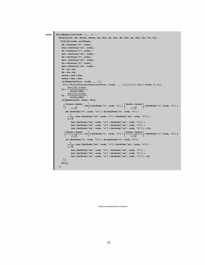
In[34]:= BuildEquations node : _, _ : �

Module Av, Ah, Anwse, Aswne, Ae, Ane, An, Anw, Aw, Asw, As, Ase, Frc, Fx, Fy ,

If PinP node, actShape ,

Ae � GetArea "e", node ;

Ane � GetArea "ne", node ;

An � GetArea "n", node ;

Anw � GetArea "nw", node ;

Aw � GetArea "w", node ;

Asw � GetArea "sw", node ;

As � GetArea "s", node ;

Ase � GetArea "se", node ;

Av � An � As;

Ah � Ae � Aw;

Anwse � Anw � Ase;

Aswne � Asw � Ane;

If MemberQ Frcs, node, _, _ ,

Frc � Frcs Flatten Position Frcs, node, _, _ 1 , Frc � node, 0, 0 ;

Fx �Frc 2 � dist

� � � � � � � � � � � � � � � � � � � � � � � � � � � � � � � �� elasticMod

;

Fy �Frc 3 � dist

� � � � � � � � � � � � � � � � � � � � � � � � � � � � � � � �� elasticMod

;

If MemberQ ZD, node , Null,

Anwse � Aswne� � � � � � � � � � � � � � � ��

2 2

� Ah � GetNode "c", node, "u" � Aswne � Anwse� � � � � � � � � � � � � � � ��

2 2� GetNode "c", node, "v" �

Aw GetNode "w", node, "u" � Ae GetNode "e", node, "u" �

1� � � � � � � � � � � � � �

2 2Asw GetNode "sw", node, "u" � GetNode "sw", node, "v" �

Ase GetNode "se", node, "u" � GetNode "se", node, "v" �

Anw GetNode "nw", node, "u" � GetNode "nw", node, "v" �

Ane GetNode "ne", node, "u" � GetNode "ne", node, "v" � Fx,

Anwse � Aswne� � � � � � � � � � � � � � � ��

2 2

� Av � GetNode "c", node, "v" � Aswne � Anwse� � � � � � � � � � � � � � � ��

2 2� GetNode "c", node, "u" �

As GetNode "s", node, "v" � An GetNode "n", node, "v" �

1� � � � � � � � � � � � � �

2 2Asw GetNode "sw", node, "u" � GetNode "sw", node, "v" �

Ase GetNode "se", node, "u" � GetNode "se", node, "v" �

Anw GetNode "nw", node, "u" � GetNode "nw", node, "v" �

Ane GetNode "ne", node, "u" � GetNode "ne", node, "v" � Fy

,

Null

;


45

Create the matrices

In[35]:= possibleNodes � Partition Flatten Table x, y , y, minY, maxY , x, minX, maxX , 2 ;

eqs � DeleteCases Flatten Map BuildEquations, possibleNodes , Null ;

var � DeleteCases

Flatten Thread Map GetUNode, possibleNodes , Map GetVNode, possibleNodes , 0 ;

mat, vec � LinearEquationsToMatrices eqs, var ;

Solve the System

In[39]:= Lsolution � LinearSolve mat, vec ;

solution � Solve eqs, var

Out[40]= u2 �� 0.000873342, v2 �� 0.00511063, u3 �� 0.0008673, v3 �� 0.00838378, u4 � 2.38894 � 10 � 19,v4 �� 0.0142231, u5 � 0.0008673, v5 �� 0.00838378, u6 � 0.000873342, v6 �� 0.00511063,u8 � 0.000876675, v8 �� 0.00222631, u9 � 0.00122874, v9 �� 0.00503332, u10 � 0.0010726,

v10 �� 0.00840954, u11 � 1.8094 � 10 � 18, v11 �� 0.0104327, u12 �� 0.0010726, v12 �� 0.00840954,u13 �� 0.00122874, v13 �� 0.00503332, u14 �� 0.000876675, v14 �� 0.00222631, u15 � 0.00185675,v15 �� 0.00329847, u16 � 0.00188014, v16 �� 0.00535986, u17 � 0.00126546, v17 �� 0.00758479,

u18 � 3.90311 � 10 � 18, v18 �� 0.00859663, u19 �� 0.00126546, v19 �� 0.00758479,u20 �� 0.00188014, v20 �� 0.00535986, u21 �� 0.00185675, v21 �� 0.00329847, u22 � 0.00292269,v22 �� 0.00356459, u23 � 0.00265657, v23 �� 0.00527127, u24 � 0.00164961, v24 �� 0.00694416,

u25 � 5.82442 � 10 � 18, v25 �� 0.00765334, u26 �� 0.00164961, v26 �� 0.00694416,u27 �� 0.00265657, v27 �� 0.00527127, u28 �� 0.00292269, v28 �� 0.00356459

Show the Solution

In[41]:= GetActualNode node : _, _ : � If PinP node, actShape , If MemberQ ZD, node , Null, node , Null ;


46

In[42]:= ScaleDisp � 30;

points � Partition Flatten var . solution , 2 � ScaleDisp �

DeleteCases Map GetActualNode, possibleNodes , Null ;

cells � ListPlot

Join points, ZD ,

AspectRatio � Automatic, Axes � True, PlotStyle � PointSize 0.02 ;

1 2 3 4 5 6-0.5

0.5

1

1.5

2

2.5

In[45]:= � Plot the original polygon over the cells �

Show Graphics RGBColor 1, 0, 0 , Line Join actShape, First actShape ,

cells ;


47

Compute the Spectral Radius

In[46]:= SpectralRadius A_ : � Max Abs Eigenvalues A ;

NonDiag x_, y_ : � If x �� y, 0,

If EvenQ x ,

If x�y � 1, mat x, y , 0 ,

If x�y � 1, mat x, y , 0

;

Diag x_, y_ : � If x �� y,

mat x, y ,

If EvenQ x ,

If x � y � 1, mat x, y , 0 ,

If x � y � 1, mat x, y , 0

;

In[49]:= sz � Length mat ;

lwr � LowerDiagonalMatrix NonDiag, sz ;

upr � UpperDiagonalMatrix NonDiag, sz ;

dg � Array Diag, sz, sz ;

Bjacobi �� Inverse dg . lwr � upr ;

Bgs �� Inverse dg � lwr .upr;

SpectralRadius Bjacobi

SpectralRadius Bgs

Out[55]= 0.979368

Out[56]= 0.959006


48

Vita

Douglas was born on July 1, 1970 in San Bernadino, California. He spent four years in

the Marine Corps which included a brief tour of Kuwait during the Gulf War. He earned a

BS degree in computer science in 1997 from Ohio Northern University. He has worked as

a programmer at LTV Steel and POMS Inc.

49

structural design using cellular automata - digital library and

Documents