i

Structural Features in Heat Transfer Modeling of

PEM Fuel Cell Materials

by

Steven Joseph Botelho

A thesis submitted in conformity with the requirements

for the degree of Masters of Applied Science

Department of Mechanical and Industrial Engineering

University of Toronto

© Copyright by Steven Joseph Botelho 2014

ii

Structural Features in Heat Transfer Modeling of

PEM Fuel Cell Materials

Steven Joseph Botelho

Masters of Applied Science

Department of Mechanical and Industrial Engineering

University of Toronto

2014

Abstract

In this thesis, the impact of incorporating high resolution structural features into the thermal

modeling of the polymer electrolyte membrane (PEM) fuel cell gas diffusion layer (GDL) and

microporous layer (MPL) is studied. Atomic force microscopy (AFM) has been used to image

the surfaces of untreated Toray GDL fibres, and the nano-sized particles within Sigracet MPL.

The validity of the GDL smooth fibre assumption commonly employed in literature is studied

using a thermal resistance network approach. The MPL, which has been found to show structural

variability between manufacturers, was also analyzed using AFM to obtain distributions for the

particle size and filling radius. The equivalent thermal resistance between MPL particles was

computed using the Gauss-Seidel iterative method, and was found to be sensitive to the particle

separation distance and filling radius. Finally, unit-cell analysis is presented as a methodology

for incorporating MPL nano-features into modeling of the MPL bulk regions.

iii

Acknowledgments

Firstly, I would like to thank God above all, for giving me this opportunity, and providing me

with the challenges I have faced on a daily basis that made me who I am today. I would like to

thank my dear professor, Dr. Aimy Bazylak, for taking me under her wing and helping me

unlock my potential. Thank you for your guidance, wisdom, and encouragement.

Thank you to my lab mates. Your eagerness to help me has bettered myself as a researcher,

student, and most importantly, as a person. Thank you James for your unlimited patience with

me from the first day I joined this group. I appreciate you answering all of my questions, even

when you were incredibly busy – and always being ready for a Dominion break. Thank you

Ronnie for overviewing my work, and helping me keep things in perspective. Those laughs we

shared when watching stupid videos together would work better than coffee during those

stressful 14 hour days.

Thank you to my family. My parents, you mean the world to me, and everything I do is with the

intention of supporting your Florida retirement. Your hard work has truly inspired me. To my

brother, Zander, thank you for being patient with me when I would hog the computer. To my

sister, Stephanie, thank you for paving the path for me to follow. I have been influenced by you

since I was a kid, and I appreciate you in my life very much. To my brother-in-law, Danny, thank

you for helping me – whether it was by picking me up from school, playing basketball with me,

or listening to my research problems, thank you. Your insight has been truly valuable. To

Rachel, the love of my life, thank you for your support during these stressful times. I appreciate

you being here for me day after day, and always believing in me. To my friends; Vahid in

iv

particular, thank you for being there for me. I have enjoyed the come-up, and I am excited to see

what the view looks like from the top.

To my best friend, Atlas. I love you, and coming home to you wiggling down the stairs at any

time of the day/night would always put a smile on my face. You are the best dog ever.

Thank you to the University of Toronto, NSERC, and OGS for all of the financial support. It is

greatly appreciated, and realistically, none of this work could have been done without your

assistance.

v

Table of Contents

Acknowledgements iii

Table of Contents v

List of Tables x

List of Figures xii

Abbreviations & Nomenclature xvii

Chapter 1: Introduction 1

1.1 Preamble 1

1.2 Motivation and Objective 2

1.3 Contributions 3

1.3.1 Journal Manuscripts 3

1.3.2 Conference Papers (Accompanied by Oral Presentations) 3

1.4 Organization of Thesis 4

Chapter 2: Background and Literature Review 5

2.1 Introduction 5

2.2 PEM Fuel Cells 5

2.2.1 Electrochemical Energy Generation 6

2.2.2 Thermal Energy and Water Management 7

2.3 Cathode Material Structure and Function 8

2.3.1 GDL Structure 8

vi

2.3.2 MPL Structure 9

2.4 Effective Thermal Conductivity 11

2.4.1 GDL Effective Thermal Conductivity 12

2.4.2 MPL Effective Thermal Conductivity 13

2.5 Tables 15

2.6 Figures 16

Chapter 3: GDL Fibre Surface Morphology 21

3.1 Introduction 21

3.2 Motivation and Objective 21

3.3 Characterization of GDL Fibre Surfaces 23

3.4 Methodology 25

3.4.1 Determination of Fibre Contact Force Range 26

3.4.2 Surface Fitting of GDL Fibre Data 27

3.4.3 Determination of Micro-Contact Order 28

3.5 Contact Mechanics 29

3.5.1 Micro-Contact Shape 29

3.5.2 Step-Wise Compression 30

3.6 Thermal Analysis 32

3.7 Rough Fibre Contact Area 34

3.7.1 Micro-Contact Area 34

3.7.2 Total Contact Area 35

3.7.3 Curve-Fitting of Total Contact Area Data 36

vii

3.8 Rough Fibre Thermal Contact Resistance 37

3.8.1 Thermal Contact Resistance Range 37

3.8.2 Critical Regions in GDL with respect to Thermal Contact

Resistance

38

3.8.3 Curve-Fitting of Thermal Contact Resistance Data 38

3.9 Conclusions 39

3.10 Tables 41

3.11 Figures 45

Chapter 4: Characterization of the MPL 58

4.1 Introduction 58

4.2 Motivation and Objective 58

4.3 Characterization of MPL Materials 60

4.4 Thermal Model 62

4.4.1 Thermal Model Description 62

4.4.2 Thermal Model Assumptions 65

4.5 Thermal Analysis of MPL Particle Contact Types 66

4.5.1 Effect of Varying Overlapping Distance on Equivalent Thermal

Resistance

67

4.5.2 Effect of Varying Filling Radius on Equivalent Thermal Resistance 67

4.5.3 Effect of Varying Separation Distance on Equivalent Thermal

Resistance

68

4.5.4 Effect of Varying Particle Diameter Ratio on Equivalent Thermal

Resistance

68

4.6 Conclusions 69

4.7 Tables 71

viii

4.8 Figures 72

Chapter 5: Unit-Cell Analysis 90

5.1 Introduction 90

5.2 Motivation and Objective 90

5.3 Unit-Cell Reconstruction of MPL Particles 91

5.3.1 Voxel Resolution Selection Based On Unit-Cell Reconstruction

Accuracy

92

5.3.2 Voxel Resolution Selection Based On Effective Thermal

Conductivity Measurement

93

5.3.3 Irregular Unit-Cells 94

5.4 Comparison of MPL Particle Features on Unit-Cell Effective Thermal

Conductivity

94

5.4.1 Filled Contact Algorithm 95

5.4.2 SGL-10BB and SGL-10BC Regular Unit-Cells 95

5.4.3 SGL-10BB and SGL-10BC Irregular Unit-Cells 97

5.4.3.1 Irregular Unit-Cell Nomenclature 98

5.4.3.2 Irregular Unit-Cell Effective Thermal Conductivity 99

5.5 Validation of the Thermal Model presented in Section 4.4 99

5.6 Conclusions 100

5.7 Tables 102

5.8 Figures 108

Chapter 6: Conclusions 117

ix

Chapter 7: Future Work 122

7.1 GDL Fibre Surface Morphology 122

7.2 MPL Particle Analysis 123

7.3 Unit-Cell Analysis 124

References 127

x

List of Tables

Table 2-1. Summary of reported effective thermal conductivity values for GDL,

MPL, and GDL+MPL substrates.

15

Table 3-1. AFM image surface feature data.

41

Table 3-2. Properties of the GDL Carbon Fibres

42

Table 3-3. Coefficients matrix for empirical mean total contact area (µm2) and

total contact area standard deviation formulae.

43

Table 3-4. Coefficients matrix for empirically determined mean thermal contact

resistance (K(mW)-1

) and thermal contact resistance standard deviation.

44

Table 4-1. Statistical information based on the gamma probability distribution

regarding MPL particle contacts and particle connections

71

Table 5-1. Impact of voxel resolution on accuracy of BCC and FCC reconstruction

102

Table 5-2. Voxel resolution for various unit-cell reconstructions

103

Table 5-3. Effective thermal conductivity of various unit-cell configurations with

air at 80oC as the fluid-phase

104

Table 5-4. Effective thermal conductivity of various unit-cell configurations with

liquid water as the fluid-phase

105

xi

Table 5-5. Effective thermal conductivity (Wm-1

K-1

) of unsaturated SGL-10BB

irregular BCC structures, with a separation distance of 0 nm in x-, y-, and

z-directions.

106

Table 5-6. Effective thermal conductivity (Wm-1

K-1

) of unsaturated SGL-10BB

irregular FCC structures, with a separation distance of 0 nm in x-, y-, and

z-directions.

107

xii

List of Figures

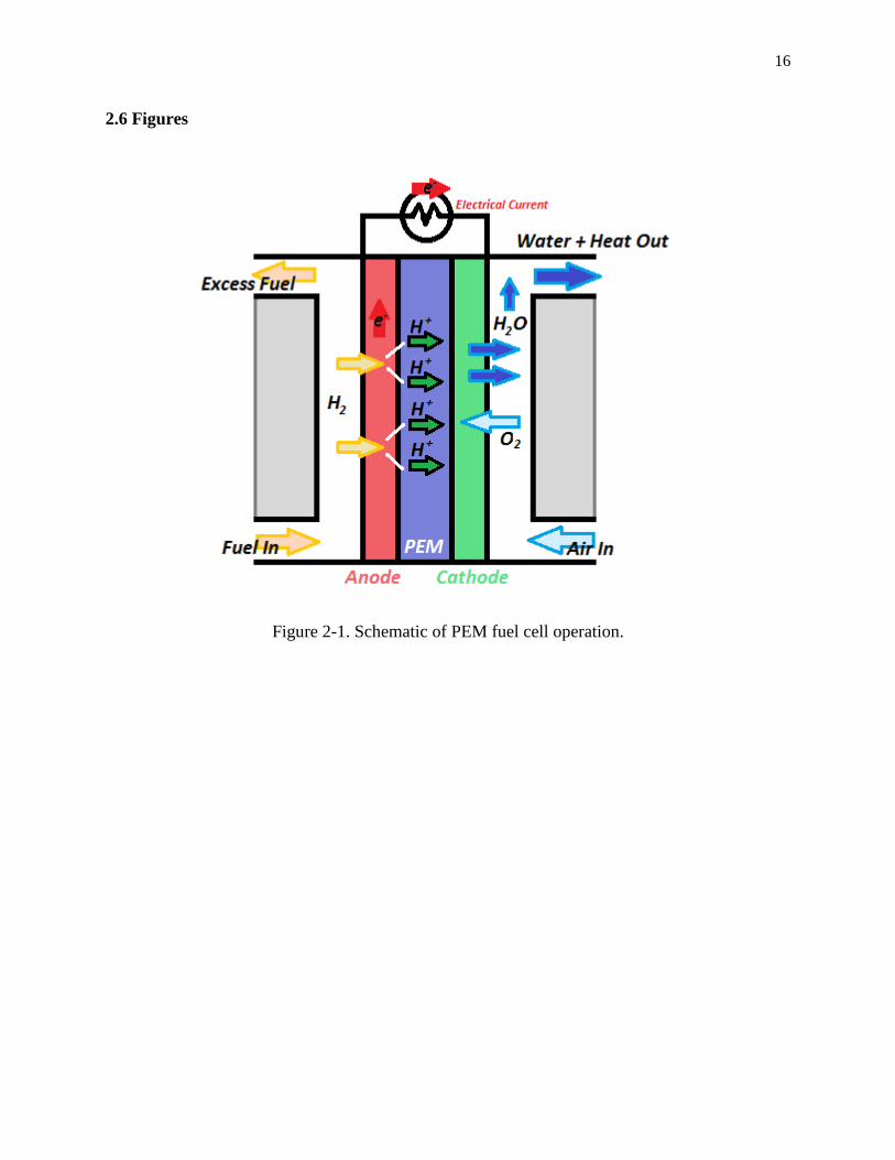
Figure 2-1. Schematic of PEM fuel cell operation.

16

Figure 2-2. SEM Image of Toray GDL.

17

Figure 2-3. Backscatter electron microscopy image comparing GDL fibre size,

MPL crack width, and MPL pore size.

18

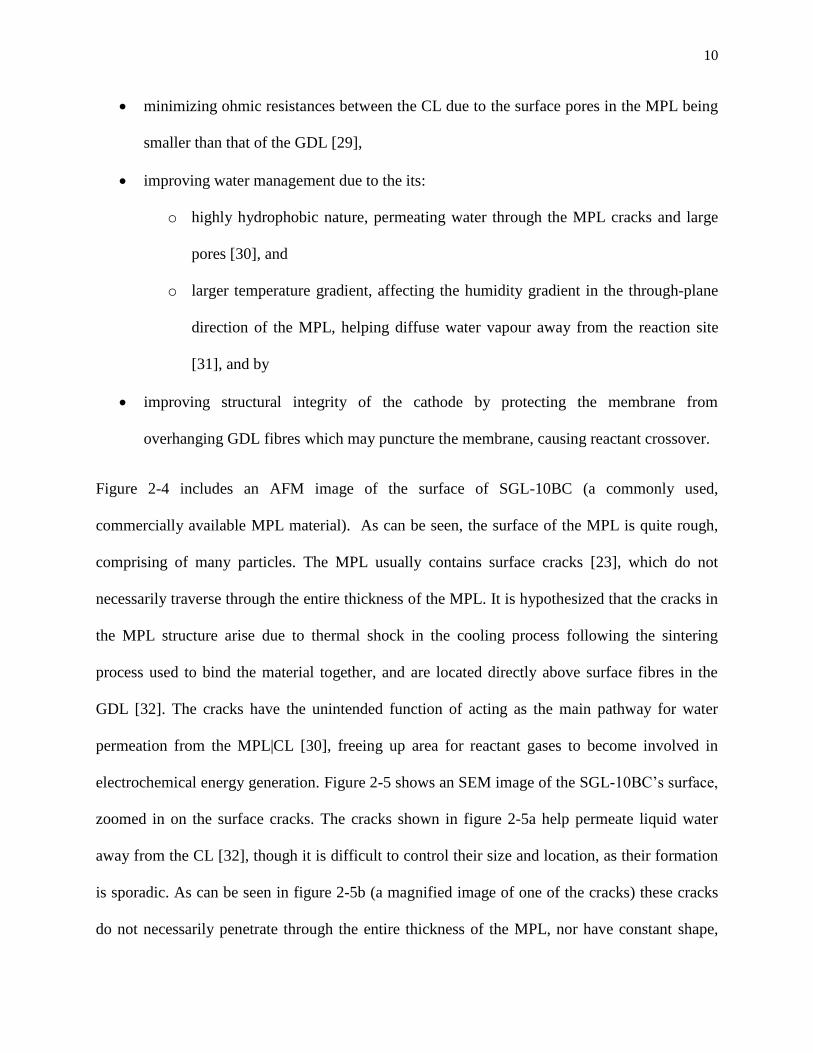
Figure 2-4. AFM images of SGL-10BC MPL with frame size of 10 μm;

Figure 2-4a) 3-dimensional view, Figure 2-4b) Topological view.

19

Figure 2-5. SEM images of SGL-10BC MPL. Figure 2-5a) 100x magnification

with scale bar length of 100 μm. Figure 2-5b) 2000x magnification on crack wall.

Figure 2-5c) 2000x magnification on crack corner.

20

Figure 3-1. AFM images used in rough contact analysis featuring cylindrical

asperities (image b and image f, respectively), protruding irregularities (image a

and image c), localized flat-zones (image e), and sharp peaks (image d).

45

Figure 3-2. 3D mapping of fibre surface data obtained using AFM for image f.

46

Figure 3-3. Height deviation in the circumferential (a), and longitudinal (b)

directions for AFM image a.

47

Figure 3-4. Algorithm used to determine thermal contact resistance and contact

area for rough contacting fibres.

48

Figure 3-5. Average Cross-Sections with and without curve fits for AFM images

a, c, and f.

49

xiii

Figure 3-6. Comparison of micro-contact shapes for two asperities of radii of

curvature equal to 100 nm in contact with various contact force, and angle of

orientation equal to (a) 45° and (b) 90°.

50

Figure 3-7. Qualitative representation of heat transfer between rough fibres.

51

Figure 3-8. Micro-contact area versus contact force for two AFM image a type

profiles in contact, for an angle of orientation of (a) 30°, (b) 45°, and (c) 90°.

52

Figure 3-9. Total Contact Area versus Contact Force for Rough and Smooth Cases

53

Figure 3-10. Total contact area versus contact force for rough and smooth cases

for an angle of orientation of 45° (a), and total contact area versus angle of

orientation for rough and smooth cases for a contact force of 0.01 N (b).

54

Figure 3-11. Average total contact area contour plot versus angle of orientation

and fibre contact force.

55

Figure 3-12. Effective thermal contact resistance versus contact force for rough

and smooth cases for an angle of orientation of 45° (a), and effective thermal

contact resistance versus angle of orientation for rough and smooth cases for a

contact force of 0.01 N (b).

56

Figure 3-13. Effective Thermal Contact Resistance versus Angle of Orientation

and Fibre Contact Force

57

Figure 4-1. SEM image of SGL-10BC showing variance in particle sizes

72

Figure 4-2 AFM images of SGL-10BB MPL with frame size of 1x1 μm2; Figure

4-2a) 3-dimensional view, Figure 4-2b) Topological view.

73

xiv

Figure 4-3: Comparison of raw AFM data (SGL-10BB) and smoothed data using a

span of 30%.

74

Figure 4-4. SGL-10BB particles (red) and particle connections (blue) circle fitted

to the smoothened AFM image height data (black).

75

Figure 4-5. Particle size distribution for SGL-10BB (a), and SGL-10BC (b).

76

Figure 4-6. Filling radius distribution for SGL-10BB (a), and SGL-10BC (b).

77

Figure 4-7. Combined data for SGL-10BB and SGL-10BC; particle size (a) and

filling radius (b)

78

Figure 4-8. Schematic of MPL particle structure (a) boundary conditions and (b)

cubic element

79

Figure 4-9. Schematic of MPL particle contact types; (a) various overlapping

distance with no filling radius, (b) various filling radius with no overlapping or

separation distance, and (c) various separation distance with constant filling

radius.

80

Figure 4-10. Schematic (a) and 3D representation (b) of particles with varying

diameter in contact. Figure 4-15b shows examples for two Dia1/Dia2: 0.4 and 1.6.

81

Figure 4-11. Equivalent thermal resistance between MPL particle contacts versus

overlapping distance.

82

Figure 4-12. Comparison of equivalent thermal resistance with air and water as the

surrounding fluid, versus overlapping distance.

83

xv

Figure 4-13. Equivalent thermal resistance between MPL particle contacts versus

filling radius.

84

Figure 4-14. Comparison of equivalent thermal resistance with air and water as the

surrounding fluid, versus filling radius.

85

Figure 4-15. Equivalent thermal resistance between MPL particle contacts versus

separation distance.

86

Figure 4-16. Comparison of equivalent thermal resistance with air and water as the

surrounding fluid as a function of particle separation distance.

87

Figure 4-17. Equivalent thermal resistance between MPL particle contacts versus

particle diameter ratio (Dia1/Dia2)

88

Figure 4-18. Particle diameter ratio distribution generated using SGL-10BB and

SGL-10BC particle size data (figure 4-5)

89

Figure 5-1. Schematic of an MPL cross-section, approximately 1 µm by 1 µm,

showing the use of unit-cells for population low-resolution MPL reconstructions

in 2D; (a) schematic of an MPL cross-section, (b) schematic of a unit-cell

populated cross section, and (c) both images overlaid.

108

Figure 5-2. BCC and FCC reconstructions using various number of voxels

109

Figure 5-3. Comparison of voxel count in unit-cell reconstruction with analytical

results for kp/km = 1000, for (a) BCC and (b) FCC structures.

110

Figure 5-4. Irregular BCC Lattice Structures

111

Figure 5-5. Irregular FCC Lattice Structures 112

xvi

Figure 5-6. Various SGL-10BB unit-cell configurations, (a) BCC with ds = 10.1

nm, (b) BCC with ds = 0 nm, (c) FCC with ds = 10.1 nm, and (d) FCC with ds = 0

nm

113

Figure 5-7. Naming system and co-ordinate axis used to define directional

effective thermal conductivities of irregular BCC (a) and FCC (b) unit-cells.

114

Figure 5-8. Comparison of numerical results with analytical data, for various

⁄ , (a) BCC and (b) FCC.

115

Figure 5-9. Analytical and numerical results for ⁄

(non-infinite), (a) BCC and (b) FCC.

116

xvii

Abbreviations & Nomenclature

PEM Fuel Cell Components:

CL Catalyst Layer

GDL Gas Diffusion Layer

MPL Microporous Layer

MPL|CL Interface between the Microporous Layer and Catalyst Layer

PTFE Polytetrafluorethylene

PEM Polymer Electrolyte Membrane

Measurement Terminology:

AFM Atomic Force Microscopy

FIB-SEM Focused Ion-Beam Scanning Electron Microscopy

LBM Lattice Boltzmann Methods

RMS Root-Mean Square

SEM Scanning Electron Microscopy

UCA Unit-Cell Analysis

Chemical Abbreviations:

e- Electrons

H2 Hydrogen Gas

O2 Oxygen Gas

H+ Protons

H2O Water

xviii

Chapter 3 Variables:

Asperity Radius

Bulk Pressure

Contact Force

TCR Effective Thermal Contact Resistance

TCRavg Effective Thermal Contact Resistance Average

TCRstd Effective Thermal Contact Resistance Standard Deviation

Fibre Thermal Conductivity

Length of Gas Diffusion Layer

Micro-Contact Radius

Micro-Contact Area

Number of Contact Points Between Layers in GDL

θ Orientation Angle

Temperature Sink

Temperature Source

Thermal Constriction Resistance

Thermal Spreading Resistance

Total Contact Area

Total Contact Area Mean

Total Contact Area Standard Deviation

Width of Gas Diffusion Layer

xix

Chapter 4 and 5 Variables:

Conductive Heat Transfer Between Elements in Direction of Initial Temperature

Gradient

Effective Thermal Conductivity Between Element i and Neighbouring Element

Effective Thermal Conductivity

Effective Thermal Conductivity of Fluid-Phase

Effective Thermal Conductivity of Solid-Phase

R Equivalent Thermal Resistance of Structure

Heat Transfer Between Element Under Consideration and Neighbouring Element

Dia1/Dia2 Particle Diameter Ratio

Separation Distance

svf Solid-Volume Fraction

Temperature Boundary Condition (top)

Temperature Boundary Condition (bottom)

Temperature of Element i

Temperature of Neighbouring Element

Thermal Conductivity of Carbon

Thermal Conductivity of Element i

Thermal Conductivity of Neighbouring Element

Thermal Conductivity of Polytetrafluoethylene

Total Heat Transfer at Structure Boundary

Unit-Cell Area

Unit-Cell Length [nm]

a Unit-Cell Length [voxels]

Voxel Area

Voxel Width

1

Chapter 1: Introduction

1.1 Preamble

Polymer electrolyte membrane (PEM) fuel cells are electrochemical energy conversion devices,

and have been a main focus of study in the area of clean energy systems in the past decade. PEM

fuel cells generate power electrochemically, utilizing hydrogen gas and oxygen from air, forming

only water and heat as by-products. Production of hydrogen gas via electrolysis or by other

alternatives is becoming more economically and ecologically efficient, with the advancement of

renewable energy systems based on solar, wind, hydro, and geothermal power generation.

With growing demand for efficient clean energy systems, PEM fuel cells offer promising

advantages over current technologies, such as the internal combustion engine, increasing their

potential as a viable alternative in energy conversion. For example, the PEM fuel cell and

internal combustion engine energy generation cycles were compared from a thermodynamic,

economic, and ecological perspective by Braga et al. [1]. In this study, it was quantitatively

determined that PEM fuel cells are more exergetically efficient (producing higher quality of

energy) than internal combustion engines, with exergetic efficiencies of PEM fuel cells being

approximately 40%, compared to 22% exergetic efficiency for internal combustion engines [1].

PEM fuel cells also produce less greenhouse gas emissions during operation, having ecological

efficiencies of 96% compared to 51% for internal combustion engines, based on the emission of

carbon dioxide [1]. Automobile companies such as Ford, General Motors, and Nissan are

committed to advancing their fleet of fuel cell based cars, with the intention of having them on

the market by 2015 [2]. However, before PEM fuel cells can compete with existing technologies

in terms of cost, durability, and reliability [1], further advancements in issues regarding thermal

2

energy and water management within the cathode of the cell must be incorporated into future cell

designs.

1.2 Motivation and Objective

The main objective of this thesis is to investigate the impact of high-resolution features in PEM

fuel cell cathode materials on their effective thermal conductivity. In particular, two cathode

materials are studied at the nano-scale: the gas diffusion layer (GDL) and microporous layer

(MPL). By understanding the impact of incorporating these features on heat transfer modeling,

more accurate predictions of effective thermal conductivity can be obtained. Using the results of

this study, thermal gradients within the cell, which affect the overall cell performance, can be

more accurately computed. The results of this study can also inform GDL and MPL

manufacturers on limiting features in their designs, helping improve their product by optimizing

material tolerances.

The impact of incorporating fibre roughness into analytically calculated fibre-fibre thermal

contact resistance is analyzed to test the validity of the smooth-fibre assumption commonly

employed in literature. Secondly, the MPL particle connections and particle sizes are studied to

investigate the variability among material types, and their impact on the numerically calculated

effective thermal conductivity, computed using the Gauss-Seidel iterative method. Finally, a

methodology for incorporating the studied nano-structures found within the MPL, based on unit-

cell analysis, is presented.

3

1.3 Contributions

The results of this work have led to the following contributions:

1.3.1 Journal Manuscripts

Botelho, S. J., and Bazylak, A. (2013) “The Impact of Fibre Surface Morphology on the

Effective Thermal Conductivity of a Polymer Electrolyte Membrane Fuel Cell Gas

Diffusion Layer”, Journal of Power Sources, 269, pgs. 385 – 395.

Botelho, S.J., and Bazylak, A. (2014) “Impact of Polymer Electrolyte Membrane Fuel

Cell Microporous Layer Nano-Scale Features on Thermal Conductance”, Journal of

Power Sources (Submitted September 2014)

Botelho, S.J., and Bazylak, A. (2014) “Development of a High-Resolution

Reconstruction of the Microporous Layer found in Polymer Electrolyte Membrane Fuel

Cells”, Journal of Power Sources (In Preparation)

1.3.2 Conference Papers (Accompanied by Oral Presentations)

Botelho, S. J., and Bazylak, A. (2013) “Development of a High Resolution Thermal

Model of the Microporous Layer found in PEM Fuel Cells” (F1-0653), Journal of

Electrochemical Society, Orlando, FL. (ECS 2015), May 11th

– 16th

.

Botelho, S. J., and Bazylak, A. (2012) “The Impact of Fibre Surface Morphology on the

Effective Thermal Conductivity of a PEM Fuel Cell Gas Diffusion Layer” (B11-1417),

Journal of Electrochemical Society, San Francisco, CA. (ECS 2014), Oct. 27th

– Nov. 1st.

1.4 Organization of Thesis

This thesis is organized into 7 chapters in total. In this chapter, a brief description regarding the

PEM fuel technology and the thesis motivation/contributions was provided. In chapter 2, details

regarding the processes required for electrochemical energy generation are described. The role of

thermal energy management and water management in the GDL and MPL, and the impact of

GDL and MPL structures on cell performance are also discussed. A detailed review of the

4

effective thermal conductivity values referenced in literature for the GDL and MPL is also

presented in chapter 2. In chapter 3, the impact of fibre surface morphology on the validity of the

smooth fibre assumption is studied by calculating the thermal contact resistance between rough

fibres. The effect of the fibre circumferential roughness, fibre orientation angle, and fibre contact

force on the contact area and thermal contact resistance is explored, with results presented in the

form of empirical relations to be used in future studies. In chapter 4, the MPL is analyzed to

obtain the particle diameter and particle connection filling radius distributions to investigate the

variability of the MPL nano-structures among different material types. The impact of

incorporating nano-resolution in the reconstruction of the MPL particles and particle connections

is explored, highlighting the effect of altering the nature of contact between particles on the

numerically calculated equivalent thermal resistance. In chapter 5, unit-cell analysis is presented

as a technique for modeling the MPL nano-features studied in chapter 4, in a macro-model of the

MPL. Finally, in chapters 6 and 7, the conclusions to the thesis and highlighted future works are

presented respectively.

5

Chapter 2: Background and Literature Review

2.1 Introduction

In this chapter, the fundamentals of PEM fuel cell operation and the impact of effective heat

transfer within the cathode on cell performance are explored. The structures of two critical

components of the PEM fuel cell, the GDL and MPL, are described and compared. Also, the

existing literature focused on effective thermal conductivity measurement and heat transfer

mechanisms within the PEM fuel cell are discussed and summarized.

2.2 PEM Fuel Cells

PEM fuel cells are electrochemical energy conversion devices that have the potential to generate

electricity with zero local greenhouse gas emissions, when fed hydrogen gas and oxygen from

air. Aside from being a clean energy system with only heat and water as by-products (when

hydrogen is used as the fuel), PEM fuel cells offer other promising advantages. For example,

PEM fuel cells maintain high efficiency during operation (50%-60% conversion efficiency) [3],

supply a high power to volume ratio (0.7 W/cm2) [3], operate with little to no noise, and are able

to quickly reach steady state conditions [4] due to their relatively low operating temperature of

80°C [5-7]. In spite of these advantages, PEM fuel cells have issues regarding their:

cost [8], primarily due to the manufacturing of the bipolar plates and use of platinum as a

catalyst to improve reaction efficiency,

durability [9], as long-term use causes decreases in mechanical stability of cell

components via crack propagation and component delamination [10], and

6

reliability [8], as maintaining steady state conditions is sometimes difficult due to their

multi-phase nature.

These limitations can be minimized by optimally designing cell components, and by designing

cathode materials for enhanced thermal energy and water management. Improvements to the

PEM fuel cell design must take place before the technology can broaden its range of viable

applications, increasing its profit margins within the booming industry of renewable energy

systems [1].

2.2.1 Electrochemical Energy Generation

The PEM fuel cell allows for continuous electrical energy conversion as long as hydrogen, H2, is

supplied to the anode, oxygen, O2, is supplied to the cathode, and operational environmental

conditions are maintained. When hydrogen is supplied to the anode of the PEM fuel cell, the

hydrogen molecule is catalytically broken down into protons, H+, that travel through the polymer

electrolyte membrane, and electrons, e-, that travel through an external circuit in the form of

electricity. When the protons and electrons meet with the oxygen molecules at the cathode

catalyst layer (CL), water is formed exothermically. The cathode half-reaction involved in the

formation of water is shown in equation 2.1. A schematic of the PEM fuel cell operation

principles is shown in figure 2-1. A detailed study regarding the amount of heat released from

the cathode half-reaction involved in water formation can be found in [11], conducted by

Ramousse et. al.

( )

7

2.2.2 Thermal Energy and Water Management

The performance of PEM fuel cells is dependent on the effective thermal energy management

and water management within the MPL and GDL. However, thermal gradients in the diffusion

media (MPL and GDL) and the saturation of liquid water are both coupled, making control of

these parameters through the design of the MPL and GDL structures quite difficult. For example,

while both heat and water are formed exothermically at the interface between the MPL and CL

(MPL|CL), heat is also produced from joule heating (ohmic resistance to electron flow in the

solid-space of the diffusion media) and water phase change [6,12]. Heat is introduced with the

inlet gases, which facilitates higher humidity in the cathode of the PEM fuel cell, helping hydrate

the polymer electrolyte membrane. Hydrating the membrane assists in minimizing fluctuations

from low to high current densities [13], as the membrane’s structural properties and ionic

conductivity (conduction of H+) are very sensitive to the membrane’s hydration levels [14,15].

Although water is required to hydrate the membrane, too much water in the MPL causes mass

transport losses (attributed to the increased tortuosity of the path reactant gases must take to the

reaction site) [16-19], causing fluctuations in current density. Also, during operation,

delamination in the MPL|CL may occur due to the fluctuation of water levels caused by

temperature changes [4]. Delamination between the MPL and CL can lead to an increase in

ohmic resistances at the MPL|CL which affects water saturation levels and the cell’s

performance [4,20]. Finally, heat sinks and sources are introduced whenever water evaporates or

condenses, respectively, which is dependent on the local saturation pressure and temperature,

further complicating the cathode temperature gradient and pathway for thermal conduction [15].

Nonetheless, there is a delicate balance between the water saturation (liquid and vapour) and

temperature levels in the PEM fuel cell which must be controlled in order to optimize

8

performance. Therefore, understanding how material structures affect heat transfer, water

permeability, and reactant gas/water vapour diffusion is critical for advancing the design of cell

components.

2.3 Cathode Material Structure and Function

The GDL and MPL are both porous materials used as domains for which the mechanical and

chemical processes required for energy generation can take place. The pore sizes in the GDL are

approximately two orders of magnitude larger than the pore sizes in the MPL. With the exception

of cracks in the MPL [21], the pore sizes in the MPL are on the order of nanometres [22] while

pore sizes in the GDL are on the order of micrometres [23,24]. The main functions of the two

materials are to assist in water management and thermal energy management through the design

of the solid-space and pore-space. In particular, the GDL and MPL designs provide:

a pathway for thermal and electrical conduction in the solid-space,

a path for inlet gas diffusion in the pore-space,

a pathway for liquid water permeation through pore-space, and

structural integrity to the design of the PEM fuel cell.

2.3.1 GDL Structure

The GDL is composed of carbon fibres, with mean diameter of 7.32 µm [5,20,25], which are

often bound together using a polymeric binding agent to improve the structures stability and

effective thermal conductivity (by increasing the contact area between fibres). The GDL fibres

are coated with polytetrafluorethylene (PTFE) to increase the structure’s hydrophobicity. The

GDL is located between the bipolar plates and CL. GDLs come in three different structures;

paper, cloth, and felt, with paper being most popular of the three structures due to its ease of

9

manufacturing and its ability to be modeled easily (consisting of stacked, relatively straight

fibres), helping its design evolve more quickly [7,26,27]. Carbon is used in the GDL structure

due to its exceptional mechanical properties, including a high stiffness to density ratio, and high

thermal/electrical conductivity. The thickness of the GDL is approximately 200 µm. Figure 2-2

includes a scanning electron microscopy image of a commercially available Toray GDL,

illustrating the random nature of the GDL structure and size-scale of the fibres.

2.3.2 MPL Structure

The MPL is a nano-porous material, composed of agglomerations of carbon particles which

range in diameter (on the order of nanometres), bound together with PTFE filling, with the

features of the MPL being two orders of magnitude smaller than that of the GDL. Figure 2-3

includes a backscatter electron microscopy image showing the relative size of the MPL

solid-space, GDL fibre, and MPL cracks. The MPL is usually coated onto one side of the GDL

near the CL, acting as either a:

fully-immersed coating, where the MPL exists within the pore-space of the GDL,

partially-immersed coating, where part of the MPL is within the GDL pore-space and the

other part is its own layer, or

standalone structure [6].

The MPL is a relatively new material structure used in PEM fuel cell operation with growing

interest as studies have shown that the incorporation of an MPL improves cell performance

(current density and voltage potential) [28]. Though the direct impact of the MPL is somewhat

unknown, it has been postulated that the MPL improves cell performance by:

10

minimizing ohmic resistances between the CL due to the surface pores in the MPL being

smaller than that of the GDL [29],

improving water management due to the its:

o highly hydrophobic nature, permeating water through the MPL cracks and large

pores [30], and

o larger temperature gradient, affecting the humidity gradient in the through-plane

direction of the MPL, helping diffuse water vapour away from the reaction site

[31], and by

improving structural integrity of the cathode by protecting the membrane from

overhanging GDL fibres which may puncture the membrane, causing reactant crossover.

Figure 2-4 includes an AFM image of the surface of SGL-10BC (a commonly used,

commercially available MPL material). As can be seen, the surface of the MPL is quite rough,

comprising of many particles. The MPL usually contains surface cracks [23], which do not

necessarily traverse through the entire thickness of the MPL. It is hypothesized that the cracks in

the MPL structure arise due to thermal shock in the cooling process following the sintering

process used to bind the material together, and are located directly above surface fibres in the

GDL [32]. The cracks have the unintended function of acting as the main pathway for water

permeation from the MPL|CL [30], freeing up area for reactant gases to become involved in

electrochemical energy generation. Figure 2-5 shows an SEM image of the SGL-10BC’s surface,

zoomed in on the surface cracks. The cracks shown in figure 2-5a help permeate liquid water

away from the CL [32], though it is difficult to control their size and location, as their formation

is sporadic. As can be seen in figure 2-5b (a magnified image of one of the cracks) these cracks

do not necessarily penetrate through the entire thickness of the MPL, nor have constant shape,

11

though that is how they are commonly modelled [29,33]. Also, the walls of the cracks are rough,

which would affect the advancing contact angle of liquid water traversing through the thickness

of the MPL away from the MPL|CL. Figure 2-5c is a magnified image of one of the crack

corners. As can be seen, there also exists over-hanging MPL particle agglomerations in the void

regions of the structure, which make up the MPL solid-space.

Though the MPL assists in water management in the PEM fuel cell, due to the high PTFE

content, incorporation of a MPL tends to lower the overall effective thermal conductivity of the

diffusion media [8]. Therefore, there is a growing interest in optimizing the design of the MPL

structure via computational modeling [21,34]. However, due to the structures variability among

manufacturer and material type, validation of MPL models is difficult [22].

2.4 Effective Thermal Conductivity

In order to analyze how well various GDLs and MPLs conduct heat, their effective thermal

conductivity is measured. Measurements have been obtained experimentally and numerically

through the use of modeling of the diffusion media structures. It has been found that the GDL

fibrous substrate effective thermal conductivity varies between the through-plane and in-plane

directions [35] while the MPL displays isotropic effective thermal conductivity and diffusion

properties [22]. Due to both the variability in the MPL structure [22] and difficulties in

distinguishing between the GDL and partially-immersed MPL structures, the reported effective

thermal conductivities range drastically [22]. Table 2-1 includes a summary of the findings in

literature for the effective thermal conductivities of the GDL, MPL, and GDL+MPL substrates.

12

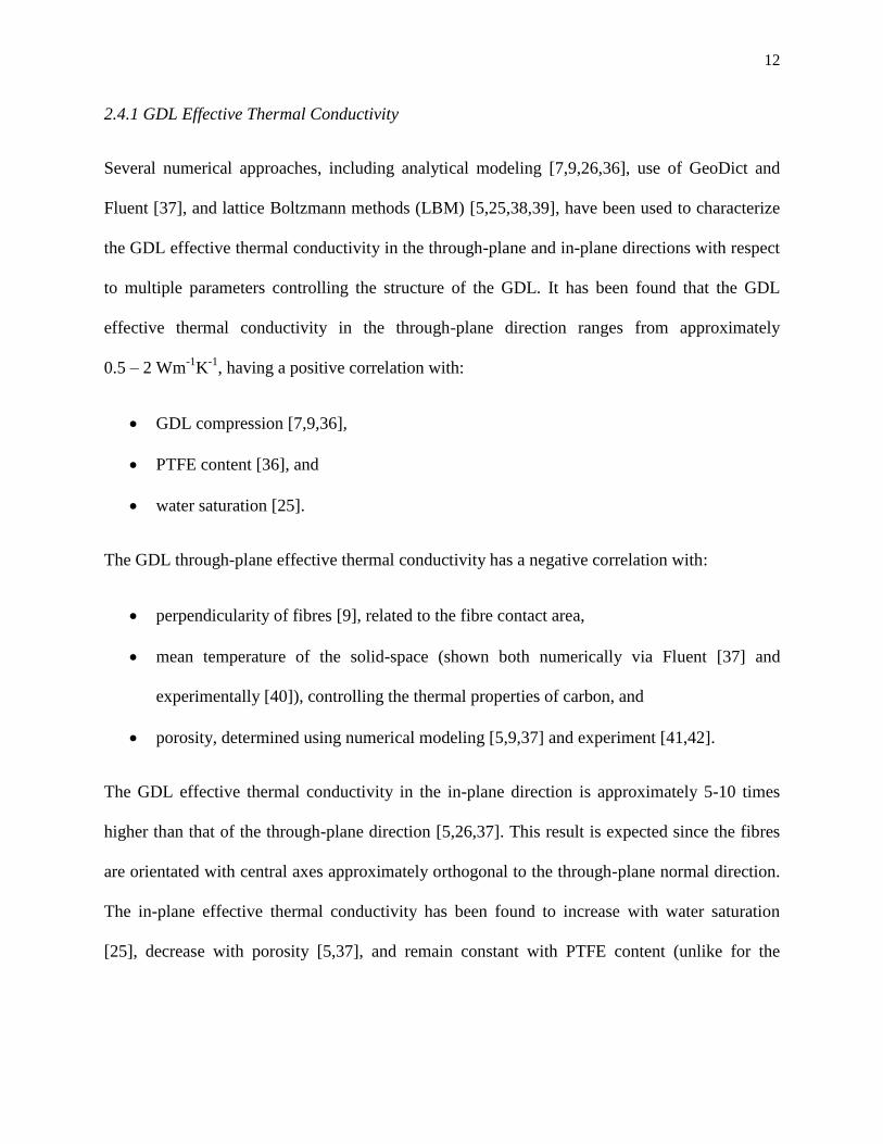
2.4.1 GDL Effective Thermal Conductivity

Several numerical approaches, including analytical modeling [7,9,26,36], use of GeoDict and

Fluent [37], and lattice Boltzmann methods (LBM) [5,25,38,39], have been used to characterize

the GDL effective thermal conductivity in the through-plane and in-plane directions with respect

to multiple parameters controlling the structure of the GDL. It has been found that the GDL

effective thermal conductivity in the through-plane direction ranges from approximately

0.5 – 2 Wm-1

K-1

, having a positive correlation with:

GDL compression [7,9,36],

PTFE content [36], and

water saturation [25].

The GDL through-plane effective thermal conductivity has a negative correlation with:

perpendicularity of fibres [9], related to the fibre contact area,

mean temperature of the solid-space (shown both numerically via Fluent [37] and

experimentally [40]), controlling the thermal properties of carbon, and

porosity, determined using numerical modeling [5,9,37] and experiment [41,42].

The GDL effective thermal conductivity in the in-plane direction is approximately 5-10 times

higher than that of the through-plane direction [5,26,37]. This result is expected since the fibres

are orientated with central axes approximately orthogonal to the through-plane normal direction.

The in-plane effective thermal conductivity has been found to increase with water saturation

[25], decrease with porosity [5,37], and remain constant with PTFE content (unlike for the

13

through-plane direction) [26]. Nonetheless, the GDL has been modeled quite extensively, and the

findings in literature have been used to further develop the structures of these materials.

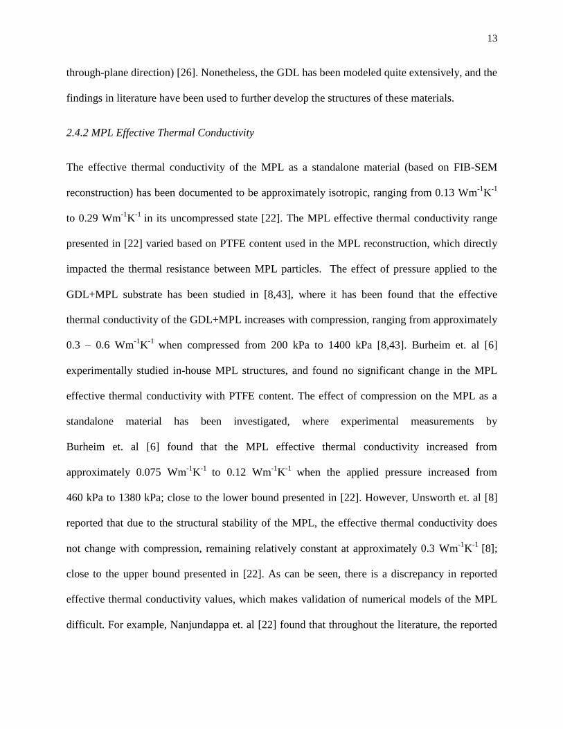
2.4.2 MPL Effective Thermal Conductivity

The effective thermal conductivity of the MPL as a standalone material (based on FIB-SEM

reconstruction) has been documented to be approximately isotropic, ranging from 0.13 Wm-1

K-1

to 0.29 Wm-1

K-1

in its uncompressed state [22]. The MPL effective thermal conductivity range

presented in [22] varied based on PTFE content used in the MPL reconstruction, which directly

impacted the thermal resistance between MPL particles. The effect of pressure applied to the

GDL+MPL substrate has been studied in [8,43], where it has been found that the effective

thermal conductivity of the GDL+MPL increases with compression, ranging from approximately

0.3 – 0.6 Wm-1

K-1

when compressed from 200 kPa to 1400 kPa [8,43]. Burheim et. al [6]

experimentally studied in-house MPL structures, and found no significant change in the MPL

effective thermal conductivity with PTFE content. The effect of compression on the MPL as a

standalone material has been investigated, where experimental measurements by

Burheim et. al [6] found that the MPL effective thermal conductivity increased from

approximately 0.075 Wm-1

K-1

to 0.12 Wm-1

K-1

when the applied pressure increased from

460 kPa to 1380 kPa; close to the lower bound presented in [22]. However, Unsworth et. al [8]

reported that due to the structural stability of the MPL, the effective thermal conductivity does

not change with compression, remaining relatively constant at approximately 0.3 Wm-1

K-1

[8];

close to the upper bound presented in [22]. As can be seen, there is a discrepancy in reported

effective thermal conductivity values, which makes validation of numerical models of the MPL

difficult. For example, Nanjundappa et. al [22] found that throughout the literature, the reported

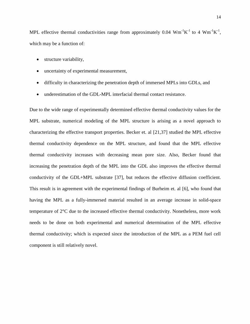
14

MPL effective thermal conductivities range from approximately 0.04 Wm-1

K-1

to 4 Wm-1

K-1

,

which may be a function of:

structure variability,

uncertainty of experimental measurement,

difficulty in characterizing the penetration depth of immersed MPLs into GDLs, and

underestimation of the GDL-MPL interfacial thermal contact resistance.

Due to the wide range of experimentally determined effective thermal conductivity values for the

MPL substrate, numerical modeling of the MPL structure is arising as a novel approach to

characterizing the effective transport properties. Becker et. al [21,37] studied the MPL effective

thermal conductivity dependence on the MPL structure, and found that the MPL effective

thermal conductivity increases with decreasing mean pore size. Also, Becker found that

increasing the penetration depth of the MPL into the GDL also improves the effective thermal

conductivity of the GDL+MPL substrate [37], but reduces the effective diffusion coefficient.

This result is in agreement with the experimental findings of Burheim et. al [6], who found that

having the MPL as a fully-immersed material resulted in an average increase in solid-space

temperature of 2°C due to the increased effective thermal conductivity. Nonetheless, more work

needs to be done on both experimental and numerical determination of the MPL effective

thermal conductivity; which is expected since the introduction of the MPL as a PEM fuel cell

component is still relatively novel.

15

2.5 Tables

Material Effective Thermal

Conductivity

Positive Correlation Negative Correlation

GDL (through-plane)

0.5 – 2 Wm-1

K-1

GDL compression

[7,9,36]

PTFE content [36]

Water saturation

[25]

Perpendicularity

of fibres [9]

Mean

temperature of

solid-space

[37,40]

Porosity [5,9,37]

GDL (in-plane)

5 – 15 Wm-1

K-1

[5,26,37]

Water Saturation

[25]

Porosity [5,37]

GDL+MPL 0.3 – 0.6 Wm-1

K-1

[8,43]

Substrate

compression [8,43]

Penetration depth of

MPL [6,37]

MPL (isotropic)

0.13 – 0.3 Wm-1K-1

[8,22]

0.075 – 0.12 Wm-1

K-1

[6]

GDL compression

(slight increase

reported in [6], no

increase reported

in [8])

Mean pore size

[21,37]

Table 2-1. Summary of reported effective thermal conductivity values for GDL, MPL, and

GDL+MPL substrates.

16

2.6 Figures

Figure 2-1. Schematic of PEM fuel cell operation.

17

Figure 2-2. SEM Image of Toray GDL.

18

Figure 2-3. Backscatter electron microscopy image comparing GDL fibre size, MPL crack width,

and MPL pore size.

19

a)

b)

Figure 2-4. AFM images of SGL-10BC MPL with frame size of 10 μm;

Figure 2-4a) 3-dimensional view, Figure 2-4b) Topological view.

20

a)

b)

c)

Figure 2-5. SEM images of SGL-10BC MPL. Figure 2-5a) 100x magnification with scale bar

length of 100 μm. Figure 2-5b) 2000x magnification on crack wall. Figure 2-5c) 2000x

magnification on crack corner.

21

Chapter 3: GDL Fibre Surface Morphology

3.1 Introduction

In this chapter, the impact of incorporating fibre surface morphology in the thermal analysis of

the PEM fuel cell GDL is investigated. Using atomic force microscopy (AFM), fibre roughness

in the circumferential direction is fitted to obtain asperity height information, which is used to

test the validity of the smooth fibre assumption. Greenwood’s rough contact model was

implemented to obtain the rough fibre contact area, and thermal contact resistance between

contacting rough fibres, for various contact force and angles of orientation. The analysis

conducted in this chapter provides a tool which can be used to incorporate the surface features of

GDL fibres into existing effective thermal conductivity models, representing more realistic GDL

structures.

3.2 Motivation and Objective

Numerical modeling has become a popular approach in aiding the design process of novel GDL

materials. Numerical modeling can be used to simulate the performance of PEM fuel cells with

respect to the multitude of parameters which affect the cell performance [44], which is difficult

to do via experimentation. It has been found that the dominant mechanism for thermal energy out

of the GDL is conduction through the carbon fibre network [11,39]. Several thermal conductivity

models exist for analyzing thermal conduction within the PEM fuel cell. Lattice Boltzmann

methods (LBM) have been used for determining the through-plane and in-plane thermal

conductivity of the GDL because of their ability to model complicated structures effectively, and

have been used to study both saturated [25,39] and unsaturated [35,38] GDLs. Using LBM, it

22

was found that the effective thermal conductivity of the GDL increases with water saturation,

with a more significant impact in the through-plane direction rather than the in-plane direction

[25]. Also, models based on analytical equations have been commonly used for characterizing

the effect of compression on the effective thermal conductivity of the GDL [7,36], by

characterizing the nature of contact between smooth fibres using Hertzian contact mechanics. It

was found that the thermal resistance in the GDL is dominated by the fibre-to-fibre contacts, and

the through-plane effective thermal conductivity increases linearly with GDL compression [36].

Although the effective thermal conductivity of the GDL has been studied, it was commonly

assumed that the surfaces of the carbon fibres are smooth [7,20], or that the reconstruction

resolution corresponding to the lattice spacing in LBM simulations was sufficient for modeling

heat flow between contacting fibres. However, as the development of a realistic thermal

representation of the GDL continues to evolve, the effect of fibre structural features in the GDL

are being considered. For example, the effect of fibre waviness in the longitudinal direction has

been studied in a recent publication (2014) by Sadeghifar et al. [45], showing a growing interest

in the validity of the simplistic nature of the assumptions controlling the representation of fibres;

assumed to be smooth and straight. The objective of this study is to investigate the impact of

incorporating realistic fibre surface morphology, in particular the circumferential fibre

roughness, on effective thermal conductivity measurement in GDLs. Using an analytical

approach based on Greenwood’s rough contact model [46], the thermal contact resistances and

contact areas between rough fibres housed in the GDL are analyzed and compared with smooth

fibre representations to test the validity of the smooth fibre assumption. The results of this study,

published in [47], could be incorporated into other existing effective thermal conductivity

23

models, further advancing effective thermal conductivity measurement to reflect what occurs

during PEM fuel cell operation.

3.3 Characterization of GDL Fibre Surfaces

Carbon fibres housed in untreated Toray GDL were analyzed using AFM. A Nanoscope IIIa

Multimode (Digital Instruments) atomic force microscope, located at the Canadian Centre for

Electron Microscopy at McMaster University, Ontario, was used to image Toray TGP-H-120

carbon fibre paper without polytetrafluoroethylene (PTFE) treatment. Fibres from the top layer

of the GDL were imaged to obtain the following surface feature information:

roughness in the circumferential and longitudinal directions,

surface area, and

height deviations caused by protruding asperities or irregularities.

The longitudinal roughness differs from the fibre waviness. The roughness in this context can be

viewed as the deviation in the distance between the fibre surface to the central axis of the fibre in

the direction considered (circumferential or longitudinal). The waviness however can be viewed

as the path which the central axis of the fibre follows, where a straight central axis would

correspond to a non-wavy fibre [45].

AFM images from two locations for three fibres within untreated GDL samples are shown in

figure 3-1. The six AFM images in figure 3-1 feature large and small asperities (image b and

image f, respectively), protruding irregularities (image a and image c), localized flat-zones

(image e), and sharp peaks (image d). A scanning frequency of 1.001 hertz with the atomic force

microscope in tapping mode was used to obtain the images with dimensions of 3 µm by 3 µm.

The image dimensions were determined by the expected size of the contact area shape based on

24

findings from previous studies assuming smooth fibre contact [7,20]; the contact area does not

exceed this boundary for the forces and orientation angles considered. Table 3-1 includes

statistical information regarding the surface features for each of the AFM images from

figure 3-1, including the root-mean square (RMS) roughness and surface area. Since the rough

fibres are nominally cylindrical in shape, with an assumed nominal carbon fibre diameter of

7.32 µm [20], the roughness values in table 3-1 were obtained by plane-fitting the height

information to a cylindrical plane [48]. The AFM images display roughness about the cylindrical

surface (the nominal shape of the fibre), and therefore the plane-fit represents the height

deviation with respect to the nominal diameter, and was not calculated assuming the nominal

surface was flat. The plane-fit was performed in the x-direction of the AFM images shown in

figure 3-1, as all fibres were oriented with their central axis parallel to the y-direction.

Using the AFM height data, a three-dimensional mapping of the fibre surfaces were obtained

using MATLAB. Figure 3-2 shows an example of one of the 3D meshes, for AFM image f in

figure 3-1. The image depicted in figure 3-2 includes the surface features of a section of an

individual carbon fibre found in the GDL. In the AFM images, the x- and y-axes represent the

spatial co-ordinate of the AFM image, while the z-axis represents the height of the surface. There

is an appreciable degree of roughness in the x-direction (the circumferential direction of the

fibre), as opposed to the y-direction (the longitudinal direction); this was also observed in

[49,50]. An example fibre height profile for image a is shown in figure 3-3. Equally

spaced slices were taken through the length and width of the AFM images to obtain roughness

profiles.

While the waviness of the fibres in the longitudinal direction may have an important effect on the

nature of contact between the GDL fibres and flat surfaces, such as the bipolar plate [45], the

25

focus of this work is to evaluate the fibre-to-fibre contact within the bulk region of the GDL. The

fibre roughness in the circumferential direction was found to be more impactful than the

roughness in the longitudinal direction. For example, figures 3-3a and 3-3b show the height

profiles of various cross-sections, traversing through the AFM images in the (a) circumferential

and (b) longitudinal directions for AFM image a. As can be seen in figure 3-3b, the surface is

relatively smooth along the fibre length, showing a single asperity deviation in height. Similar

trends were found for the other cases. Throughout the various AFM images, it was found that the

largest deviation in height along the longitudinal direction caused by roughness (excluding

inclusions on the fibre surface) was approximately 50 nm, which is negligible considering the

degree of roughness in the circumferential direction (figure 3-3a). Height profiles for

cross-sections at different positions along the length of the fibre are shown in figure 3-3a, and

show no significant change in cross-section. The bolded curve represents the nominal diameter

of the fibre [20] and was curve-fitted to each of the respective AFM images using a RMS

approach. As can be seen, although the cross-section is relatively constant along the 3 µm length

of the fibre, the circumferential roughness causes a significant variation from the assumed

smooth fibre profile, shown in the deviation of the rough fibre cross-sections compared to the

smooth fibre profile (bolded curve).

3.4 Methodology

An analytical approach was used to determine the contact area and thermal contact resistance

between rough fibres. Pairs of fibre surface profiles were analyzed for a range of contact forces

that would be expected within the GDL of an assembled fuel cell. A range of fibre orientation

angles from 15° to 90° was studied. The mechanical and thermal properties used in the study

26

(Table 3-2) were assumed to be isotropic. Figure 3-4 shows the algorithm used for calculating

the contact area and thermal contact resistance of GDLs.

3.4.1 Determination of Fibre Contact Force Range

The range of contact forces was determined using the results of a previous study, where Yablecki

et al. [20] developed analytical formulations for the number of contact points between adjacent

layers of fibres in compressed GDLs. These formulations were derived from micro-computed

tomography data [51] yielding porosity distributions for compressed GDLs. Using the porosity

distributions, this group numerically constructed GDLs based on the nominal diameter and

length of fibres housed in commercial GDLs, while assuming the fibres were preferentially

stacked and allowed to overlap within adjacent layers. The number of contacts between fibres in

adjacent layers was then determined using the numerically reconstructed GDLs, and presented as

a function of orientation angle and average layer interface porosity [20]. The total number of

contact points (on average) between layers within the GDL for various GDL thicknesses was

then determined [20]. The range of contact forces experienced by the fibres in contact was then

found using equation 3.1 [20], where is the contact force experienced between touching fibres

when a GDL section of length , and width is exposed to a through-plane bulk pressure

of . The bulk pressure used to compress the GDL during operation typically ranges between

460 kPa and 1390 kPa [20,52]. Though these are just bulk values, the actual pressure the GDL

will experience is dependent on the location of the GDL section (under the ribs or channel of the

bipolar plates).

( ) ( ) ⁄

27

Equation 3.1 assumes the contact force is evenly distributed among the number of contacts

between the two layers, defined as . It was found that the maximum contact force occurs

between the layers with largest porosity values. The largest contact force experienced between

contacting fibres was calculated to be 0.01 N. Therefore, this value was used as an upper-bound

when parameterizing the contact area and thermal contact resistance with the contact force. The

contact forces between fibres are difficult to verify due to the complexity of the GDL structure.

However it is hypothesized that the low contact force regions in the GDL, such as beneath the

bipolar plate channels, is best reflected by forces less than 0.002 N. Therefore, the contact force

range from 0 and 0.002 N is critical in the thermal contact resistance analysis presented in this

chapter, and is discussed in more detail in section 3.8.1.

3.4.2 Surface Fitting of GDL Fibre Data

The first step in the algorithm shown in figure 3-4 is the input of the fibre contact profiles, which

are different than the AFM images shown in figure 3-1. The fibre contact profiles represent

analytical mappings of each asperity, comprised of a diameter and position. It was assumed that

the cross-section of the fibres could be arithmetically averaged across the 3 µm length of each

AFM image, since there was no appreciable degree of roughness in the longitudinal direction.

Therefore, the protruding asperities were curve-fitted in each of the average cross-sections with

circular curves. The diameters and heights of the circular curves were obtained using a RMS

curve fit, as described in [48]. The assumption that the average cross-section could be used along

the 3 µm length of AFM images implies that the asperity surfaces are cylindrical. The curve fits

for three of the six AFM images from figure 3-1 are shown in figure 3-5.

28

3.4.3 Determination of Micro-Contact Order

Once two fibre contact profiles have been selected for analysis, the next step is to determine the

number of micro-contacts. A micro-contact is formed when an asperity of one fibre comes into

contact with an asperity of another fibre. The number of potential micro-contacts is the product

of the number of asperities for the two fibre contact profiles considered. The red asperity curve

shown for AFM image a is a special case, which will be described in detail in section 3.5.

For this study, the maximum force considered is 0.01 N, which is not large enough for the lowest

asperities to come into contact with the tallest ones. Therefore, the next step in the analysis is to

determine the order in which the micro-contacts potentially come into contact. For two

non-parallel fibres coming into contact with an angle of orientation (θ), the order of contact is

solely determined by the height of each individual asperity. In essence, the two asperities with

highest peaks will come into contact first. If fibres were to be compressed together further, a

second contact would be formed when one of the two initially contacting asperities meets the

next tallest asperity, and so on. The distinct order of the contacts can be described as the ranking

of the summed heights of all combinations of asperities for the two fibre contact profiles

considered.

Once the contact problem has been fully described using the input information of the contact

order, the angle of orientation is considered. In this study, an angle of orientation of 90° means

the projection of the central axis of the top fibre is orthogonal to the central axis of the bottom

fibre. The 0° case consisting of parallel contacting fibres is not considered in this study.

29

3.5 Contact Mechanics

The method used in this study for analysing the contact between two rough fibres is based on a

step-wise compression algorithm evolved from Greenwood’s rough contact model [46]. Since

the protruding asperities in this study are fitted with circular curves, the asperities in contact are

treated as micro cylinders, rather than spherical tips as in the Greenwood model [46]. Moreover,

since there are relatively few asperities within the 3 µm by 3 µm domain, micro-contact analysis

is performed individually rather than stochastically via probabilistic functions [33] or by using

Fourier transforms [29]. In this study, the well-established Hertzian contact mechanics

formulations [53] are used to determine the micro-contact area and fibre normal displacement

(penetration displacement), while ensuring the maximum pressure is less than the tensile strength

for the carbon fibres [54]. It is assumed that the individual asperities are smooth, continuous, and

non-conforming surfaces, which are compressed together while neglecting friction. The Hertzian

equations are valid for small strains, which lead to stresses remaining in the elastic region for

these surfaces.

3.5.1 Micro-Contact Shape

The Hertzian equations used to model the contact between the micro-cylinders, generated using

the GDL fibre asperities, can be found in chapter 4 in the work of Johnson [53]. The analytical

approach to fully characterizing the contact between two cylinders forming normal, Hertzian

elastic contact is presented and explained in detail. In order to analyze the micro-contact area

between two rough GDL fibres, the elastic modulus, Poisson ratio, contact force, radii of

curvature of the two asperities, and angle of orientation are needed. The shapes of the

micro-contacts are generally elliptical and are dependent on the orientation angle and cylinder

diameters, while the area of the micro-contacts is dependent on the contact force. For the special

30

case of the orientation angle being 90° and cylinders in contact being equal in diameter and

mechanical properties, the micro-contact shape is circular. Figure 3-6 shows an overview of the

contact shapes for two arbitrary asperities with radii of curvature equal to 100 nm and equal

mechanical properties (as would be the case for contacting GDL fibres), for various contact

forces and angles of orientation. In figure 3-6, the grey regions represent the regions of the

asperities in contact (not the entire fibre), the red dashed line represents the orientation of the

major axis of the elliptical contact area, and the green and blue + green regions represent the

contact regions for the various contact forces. The dotted black lines represent the central axis of

the two contacting cylindrical asperities. It is important to note that figure 3-6 shows an example

of a micro-contact. The actual modeled contact area between rough fibres will be comprised of

multiple micro-contacts, with varying size and shape.

3.5.2 Step- Wise Compression

The step-wise compression algorithm begins with the two highest asperities forming point

contact. At each step, the contact force is increased, and Hertzian analysis is used to determine

the contact area and normal displacement at the locations of the micro-contacts. As the contact

force continues to increase incrementally, a second micro-contact may form when the fibre

normal displacement is sufficiently large. When more than one micro-contact occurs, the

increment in contact force is distributed amongst the micro-contacts. At the instance where the

second contact is formed, the asperities forming the initial micro-contact have already been

compressed a certain amount. Therefore, in order to compensate for the elastic compression

imposed up until this point, the increment of the contact force, rather than the total contact force,

is split up evenly amongst the micro-contacts in the following iteration [55]. Therefore, it is

31

assumed that the fibres are vertically compressed into each other (without rotation about the fibre

axis), without slippage.

During each step, the contact force is incremented, the algorithm determines which asperity

combinations form micro-contacts, and Hertzian analysis is used to calculate the elliptical

micro-contact area and normal displacement of the fibres for each micro-contact. The area of

each micro-contact is calculated independently, and the effect of neighbouring asperities is

assumed to be negligible in this study since the contact forces are small [55]. The contact area

was examined to exclude overlapping micro-contact regions with the notion of macro-asperities.

In some cases, since the mean surface is curved rather than smooth, the curve fitted regular

asperities (shown in blue in figure 3-5) do not represent the rough fibre surface well. For

example, in figure 3-5, image a, the rightmost regular asperity fits the protrusion from the

surface well, but not the entire fibre profile. Macro-asperities, such as the curve shown in red in

figure 3-5, image a, are used to account for these special cases where it appears that there is an

asperity on top of an asperity. The goal of using the notion of macro-asperities is to better

approximate the contact area, and is commonly used in models comparing various magnification

levels of surfaces [56]. For example, considering AFM image a (figure 3-5) coming into contact

with a flat-surface, initially, the rightmost regular asperity (blue) will be used to define the

contact between the two surfaces. However, once the normal displacement exceeds

(approximately) 100 nm, the surface of the fibre becomes much wider, as the compression of the

regular asperity caused the flat surface to come into contact with the macro-asperity region of

the fibre. Therefore, in subsequent force increments, the properties of the macro-asperity are

used in calculating the increase in contact area and normal displacement [53]. The model

automatically utilizes the notion of macro-asperities to account for irregular surface features,

32

where smaller asperities appear to be on top of larger asperities. It is important to note that the

initial compression of the regular asperity would cause resistance to further compression once

the macro-asperity information is used in the contact advancement due to the pressure attributed

to the micro-contact. This is accounted for by appending the normal displacement of the

macro-asperity to the initial compression of the regular asperity, and by continuing to calculate

the maximum pressure (located at the centroid of the micro-contact area) using the original

regular asperity curvature.

3.6 Thermal Analysis

Once the contact area is determined, the next step is to calculate the effective thermal contact

resistance between the contacting rough fibres. The effective thermal contact resistance ( ) is

calculated using an equivalent resistance network consisting of the constriction and spreading

resistances of each of the individual micro-contacts [57]. In this study, it was assumed that the

only heat transfer occurring between the fibres was steady, thermal conduction through the

carbon solid space. Thermal conduction along the length of the fibres was not calculated, as it is

commonly assumed to be negligible in comparison to the spreading and constriction resistances

[7,9,20]. Since untreated fibres (with PTFE) were analyzed, the effect of PTFE agglomeration

near the fibre contacts was not considered. Also, the effect of interstitial fluid thermal

conductivity on the constriction/spreading resistance was not analyzed, although the thermal

conduction would be dominated by the solid pathways through the carbon material, as the carbon

thermal conductivity is much greater than that of other species found in the GDL [20]. Heat

transfer caused by convection was found to be negligible by Ramousse et al. [58] as the velocity

of fluids through the interstitial spaces and surrounding the fibres is miniscule. Radiative heat

33

transfer is negligible for temperatures below 1000 K [39], which is the case for PEM fuel cells

operating at temperatures of approximately 80°C (353 K).

Figure 3-7 depicts a representation of the thermal and mechanical phenomena occurring during

fibre contact [59]. The thermal energy is transferred between rough fibres through the

micro-contacts. Each of the micro-contacts has their own respective spreading and constriction

thermal resistances [46]. The equivalent thermal resistance network used to determine the

between two rough fibres with temperatures of and is obtained by summing the

constriction ( ) and spreading ( ) resistances in series, then by adding the sums ( + )

in parallel [46]. The formulations used to determine the thermal contact resistance for the

micro-contacts are provided by Cooper et al. [57]. Here, it is assumed that the thermal domain

can be treated as a flux-tube geometry considering the effect of neighbouring asperities [59]. The

formulation used is presented in equation 3.2, where asperity radius ( ) depends on which

asperity is forming the micro-contact, the thermal conductivity of the fibre ( ) is

120 Wm-1

K-1

, and the equivalent micro-contact radius ( ) is calculated using the micro-contact

area ( ): √ ⁄ , which is determined using the steps outlined in section 3.5.2. Once

the micro-contact areas are obtained, the thermal contact resistance per micro-contact can be

calculated using equation 3.2, from which the effective thermal contact resistance ( ) can be

computed.

( ) (

⁄ ) ( )⁄

34

3.7 Rough Fibre Contact Area

Sections 3.7 and 3.8 includes the results obtained for the analyses for contact area and thermal

contact resistance between two rough GDL fibres, respectively. Since the surface morphology

can vary between different fibres [49], there is a multitude of contact combinations which can

occur. For example, the combinations studied in this analysis could include 256 cases formed by

cross-referencing each of the AFM images, and by vertically and/or horizontally rotating fibre

contact profiles prior to the analysis. Each case was analyzed for various angles of orientation

and contact force.

3.7.1 Micro-Contact Area

Figure 3-8 depicts the micro-contact area versus contact force for the case of two fibre profiles

with AFM image a surface information coming into contact for various angles of orientation. In

these figures, each of the curves corresponds to the growth of an individual micro-contact area as

the contact force is increased. For example, since profiles shown in figure 3-8 both have two

asperities, having them come in contact will lead to 4 micro-contacts (four curves). In each of the

three sub-figures shown in figure 3-8, some micro-contacts are formed after the initial contact.

One point of interest in these figures is the change in slope of the individual contact areas. As

can be seen, the rate of change of the micro-contact area with contact force decreases as new

contacts are formed. The proportionality of the micro-contact area ( ) with the contact force

( ) in figure 3-8 is ∝

, which is in line with the results of Hertz, presented by Persson

in [56], and also mentioned in [46,60]. Also, the total contact area for this fibre contact

combination ( ), as shown in figure 3-9, tends to increase linearly with contact force (with

values larger than 0.002 N) such that ∝ , which is in agreement with contact models that

have the ability to form new contacts [56].

35

Figure 3-8 also shows the effect of altering the orientation angle on the micro-contact area; the

micro-contact area decreases as the angle of orientation approaches 90°, due to there being a

smaller projection of the top fibre onto the bottom fibre. When the asperities in contact have

equal diameter and mechanical properties (as in the case depicted in figure 3-7c), the

micro-contact shape is circular, as shown in figure 3-6. For angles of orientation of 30° and

45°, the micro-contact area shape is elliptical, yielding larger contact areas than the orthogonal

case.

3.7.2 Total Contact Area

The total contact area is a summation of the individual micro-contact areas. Figure 3-9 includes

total contact area values for the base cases depicted in figure 3-8, and as well as data for two

smooth fibres in contact (with no micro-asperities). The total contact area for the rough cases is

significantly less than the total contact area for the smooth fibre cases for fibre contact force

range and orientation angle range considered.

Figure 3-10a shows the total contact area versus the contact force at a constant angle of

orientation of 45° and versus the angle of orientation at a constant contact force of 0.01 N (figure

3-10b). In these images, the dashed line represents the smooth fibre case; fibres with no

asperities. The smooth fibre approximation is typically considered in existing effective thermal

conductivity analyses in the literature [7,9,11,20,26,38,58] and provides a good grounds for

comparison to the rough fibre cases. The solid, dark curve within the grey shaded region

represents the arithmetically calculated average total contact area amongst the various rough

fibre contact profile combinations. The shaded region represents the range exhibited throughout

the analysis, defined by the upper and lower bounds of the total contact area values. The total

36

contact area for the average rough case and its upper bound are less than the total contact area of

smooth fibres in contact. This is observed for the range of angles of orientation and contact

forces. The difference in the total contact area for the rough and smooth cases increases with

contact force.

3.7.3 Curve-Fitting of Total Contact Area Data

The total contact area is depicted in a contour graph as a function of orientation angle and the

contact force in figure 3-11. The data displayed in figure 3-11 is the average contact area

amongst the various fibre surface profile contact combinations. As can be seen, the contact area

increases with contact force, and decreases with angle of orientation (as the angle of orientation

approaches the orthogonal case of 90°). The change in contact area with angle of orientation is

more evident for larger contact forces. The average measured rough contact area data, shown in

figure 3-11, was surface-fit to obtain an empirical formulation as a function of angle of

orientation ( ) and contact force ( ). The form of the empirical average contact area

surface-fit ( ), measured in µm2, and standard deviation between measured values

( ) is displayed in equation 3.3.

( ) ( )

The constants for and are found in table 3-3. The surface fits were

determined using a least squares fit (MATLAB 2011a), and were fitted to the data within 98%

accuracy. The surface-fits for the average contact area and contact area standard deviation were

computed for the angle of orientation range considered (15° to 90°), and contact force range of

0.0001 N to 0.01 N. Note, the units for the input variables and are degrees (°) and

newtons (N) respectively. The formulation shown in equation 3.3 and table 3-3 may serve use to

37

those interested in incorporating fibre surface morphology between rough carbon fibres within

the ranges considered. Also, these formulations could be used as an input into existing effective

thermal conductivity models to incorporate surface feature information with respect to the carbon

fibres.

3.8 Rough Fibre Thermal Contact Resistance

The data for various fibre profiles in contact as a function of contact force and angle of

orientation is shown in figure 3-12a and figure 3-12b. As shown in figures 3-12a and 3-12b, the

for the average rough fibre contact is greater the smooth fibre case.

3.8.1 Thermal Contact Resistance Range

Similar to figure 3-10, the shaded regions in figure 3-12 represent the range of measured for

various fibre contact combinations. The range of rough values (shaded region in

figure 3-12a) is large, constituting to approximately 40% of the average when the contact

force is greater than 0.008 N, and approximately 90% of the average when the contact

forces are below 0.002 N. This is shown specifically in figure 3-12b, where the lower bound of

the rough approaches the smooth fibre case for an angle of orientation near 90° and high

contact forces. The of the rough GDL fibres in contact is sensitive to the shape of the total

contact area; contact areas derived from multiple smaller micro-contacts lead to thermal contact

resistances which are higher than those arising from contact areas derived from larger elliptical

shapes, leading to the variation in results presented (range of values). It was found that

the lower bound of the rough fibre range is defined by fibre profiles with larger asperities in

contact, leading to larger micro-contact areas, while the upper bound is defined by fibre profiles

with smaller asperities, leading to smaller micro-contact areas.

38

3.8.2 Critical Regions in GDL with respect to Thermal Contact Resistance

When the contact force is significantly high, the amount of compression of each of the fibres into

one another becomes significantly large, and may amount to the heights of the asperities having a

minimal effect on the overall . In essence, higher contact forces cause compression area

shapes that approach the smooth fibre case (elliptical). The opposite is true for lower contact

forces, where the surface roughness and asperity heights dominate the contact formed between

rough fibres, leading to much larger values. This is significant in the design of GDLs since

there will be various contact forces experienced by fibres underneath the bipolar plates. In the

regions below the bipolar plate ribs, there will be larger contact forces, and therefore, the effect

of fibre surface morphology will be negligible with respect to the computed . However,

underneath the channels of the bipolar plates, the contact forces will be less, and therefore the

fibre roughness should be considered in the determination of the thermal heat transfer between

contacting fibres.

3.8.3 Curve-Fitting of Thermal Contact Resistance Data

A contour plot for the thermal contact resistance versus the angle of orientation and contact force

is depicted in figure 3-13. The data in the contour plot is calculated similarly to that of

figure 3-11, being the arithmetic average of the various fibre profile contact combinations with

varying contact force and angle of orientation. The force axis is displayed in a logarithmic

fashion, as there are larger gradients in thermal contact resistance for lower contact forces. The

tends to increase with decreasing contact force and as the angle of orientation approaches

the orthogonal case. Also, the change in with angle of orientation is more evident for

contact forces below 0.001 N; an opposite trend to that shown in the contact area contour in

39

figure 3-11. Equation 3.4 shows the empirical form for the effective thermal contact resistance

average values ( ), measured in K(mW)-1

(degrees kelvin per milliwatt), and the standard

deviation ( ). The standard deviation is calculated similarly to that of contact area standard

deviation, . Empirical formulations for the were derived using MATLAB, in a

similar manner to those derived for the total contact area found in equation 3.3. The coefficients

to the two empirical surface-fits are tabulated in table 3-4, and are valid for angles of orientation

of 15° to 90°, and contact forces of 0.0001 N to 0.01 N. The formulations shown in equation 3.4

and table 3-4 provide a tool used to reproduce the analysis conducted for rough contact between

GDL fibres. It is important to note that the thermal contact resistance reported is solely due to the

conduction through the solid space of the contact carbon asperities. Results from the study

may be used in analyses with other materials within the contact region (such as PTFE, binder, or

interstitial fluid) causing other thermal contact resistances, though care must be taken in

summing the resistance values. The analysis conducted provides insight into the effect of

incorporating the circumferential fibre roughness in computed thermal contact resistance, and

also provides an alternative to increasing the grid resolution when considering the fibre

structures in GDL models.

( ) ( )

( )

3.9 Conclusion

In this study, a method for determining the contact area between rough fibres for various angles

of orientation and contact load was presented. Fibre surface information was obtained using

AFM for untreated Toray carbon paper (TGP-H-120) GDL samples with 0% PTFE content. A

modification of the Greenwood rough contact model, treating the asperities as cylindrical tips

40

(rather than the classical use of spherical tips), was used to determine the contact area between

rough fibres. It was found that the contact area of rough fibres housed in the GDL changes

with angle of orientation, with minimum values when the contacting fibres are

orthogonal. The contact area of rough fibres was found to be less than the analogous smooth

fibre case for various angles of orientation and contact force, with larger deviations for higher

contact forces.

It was found that the thermal contact resistance decreases with increasing contact force, with

maximum points at angles of orientations of 90°. The effect of fibre surface morphology on

thermal contact resistance calculations is more significant for lower contact forces, such as those

imposed on fibres underneath the bipolar plate channels. Empirical formulations for the contact

area and thermal contact resistance were presented, and were found to be within 98% accuracy of

the average contacting fibre surface. The goal of this work was to determine the impact of the

smooth-fibre assumption, and it was found that the circumferential roughness features do have a

significant impact on the contact area and thermal contact resistance between fibres. Fuel cell

modellers are encouraged to incorporate these circumferential roughness features into their bulk

(macro) GDL models, which should then result in more predictive thermal conductivity values

that can be compared to experimental validation work.

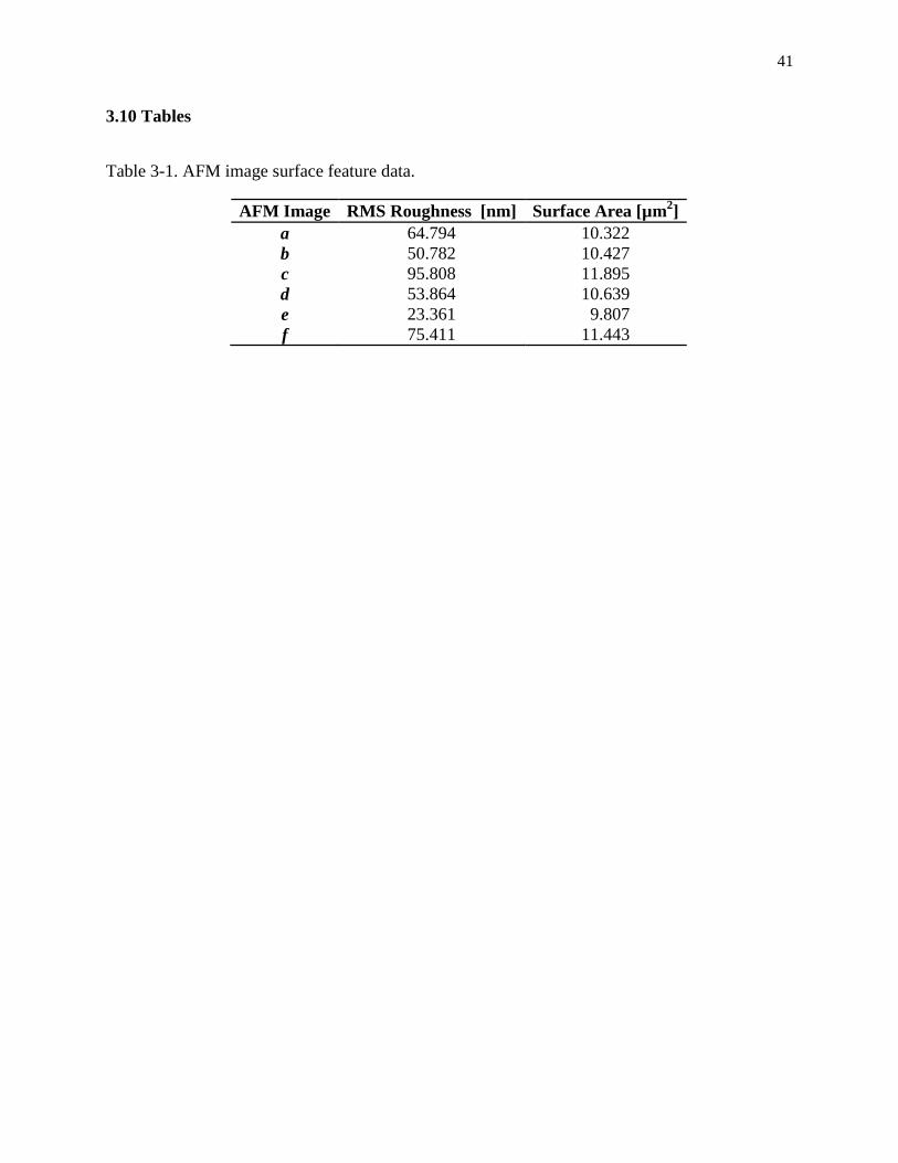
41

3.10 Tables

Table 3-1. AFM image surface feature data.

AFM Image RMS Roughness [nm] Surface Area [µm2]

a

b

c

d

e

f

64.794

50.782

95.808

53.864

23.361

75.411

10.322

10.427

11.895

10.639

9.807

11.443

42

Table 3-2. Properties of the GDL Carbon Fibres

Average Fibre

Diameter,

Average Fibre

Length, Thermal

Conductivity,

Poisson’s

Ratio,

Young’s Modulus of

Elasticity,

7.32 µm [20] 325 µm [20] 120 Wm-1

K-1

[20] 0.3 [9] 210 GPa [9]

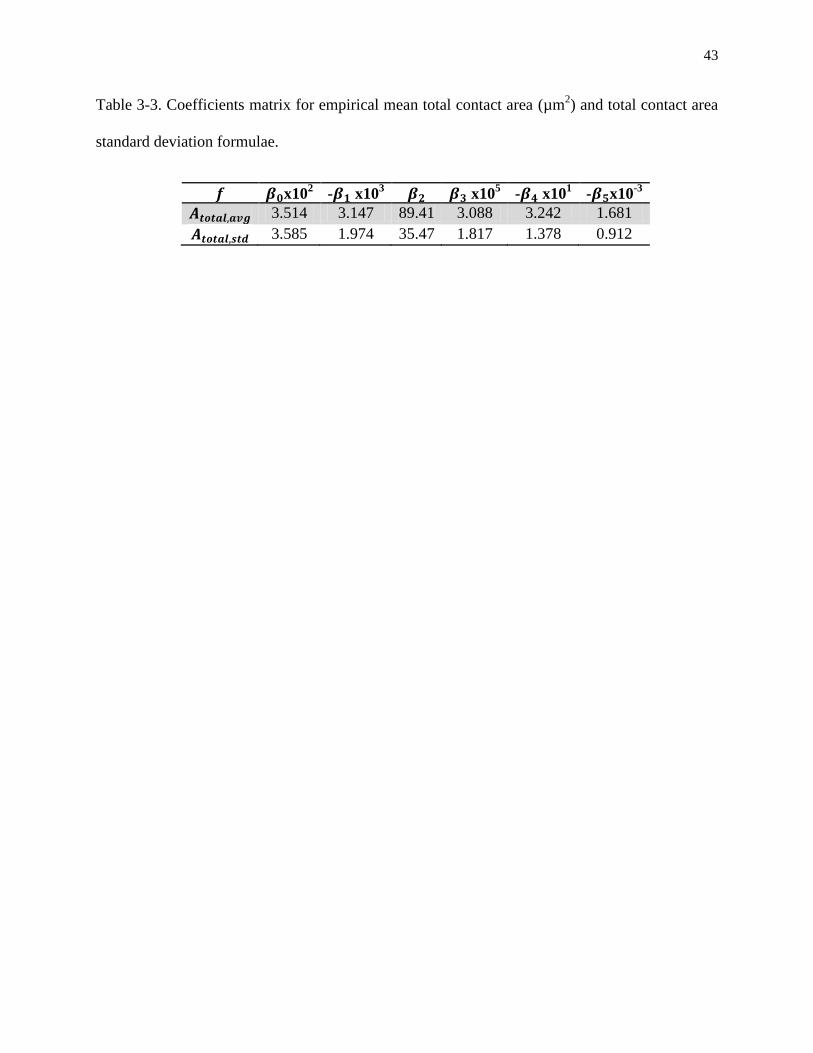
43

Table 3-3. Coefficients matrix for empirical mean total contact area (µm2) and total contact area

standard deviation formulae.

x102

- x103 x10

5 - x10

1 - x10

-3

3.514 3.147 89.41 3.088 3.242 1.681

3.585 1.974 35.47 1.817 1.378 0.912

44

Table 3-4. Coefficients matrix for empirically determined mean thermal contact resistance

(K(mW)-1

) and thermal contact resistance standard deviation.

- x10

2 x10

2 - x10

1

1.553 1.049 2.98 1.652 1.27 97.42

1.327 -6.530 2.50 -0.507 0.98 58.43

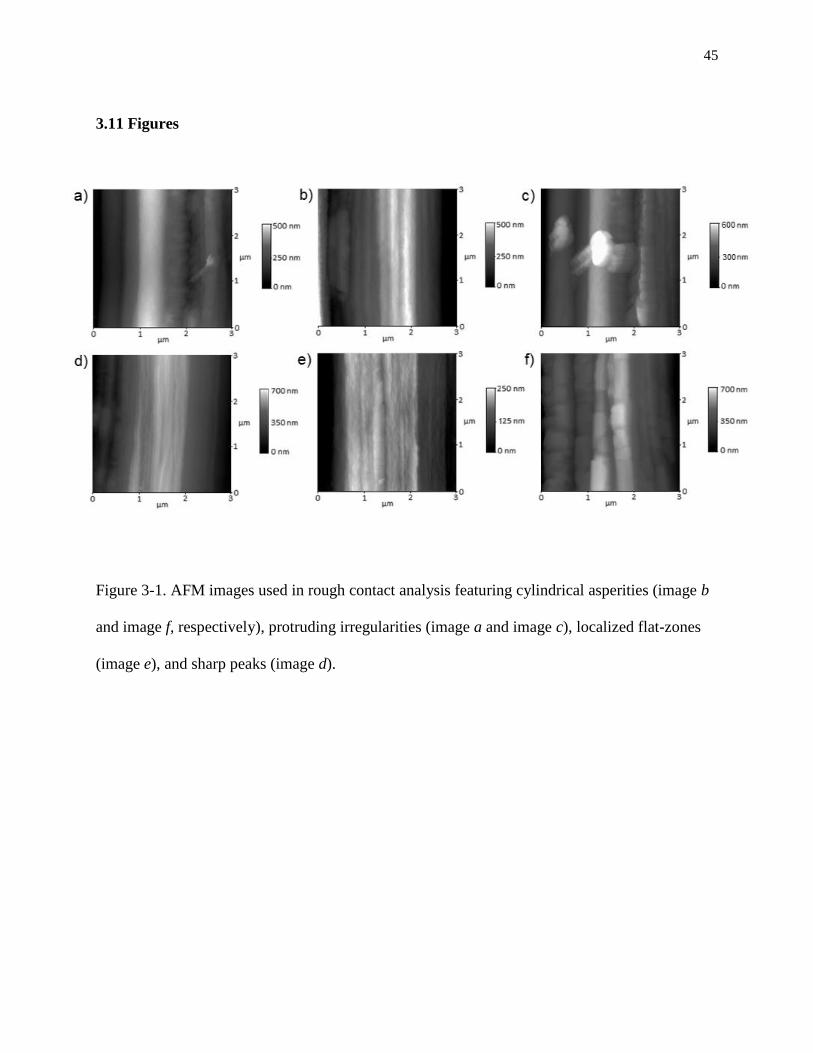
45

3.11 Figures

Figure 3-1. AFM images used in rough contact analysis featuring cylindrical asperities (image b

and image f, respectively), protruding irregularities (image a and image c), localized flat-zones

(image e), and sharp peaks (image d).

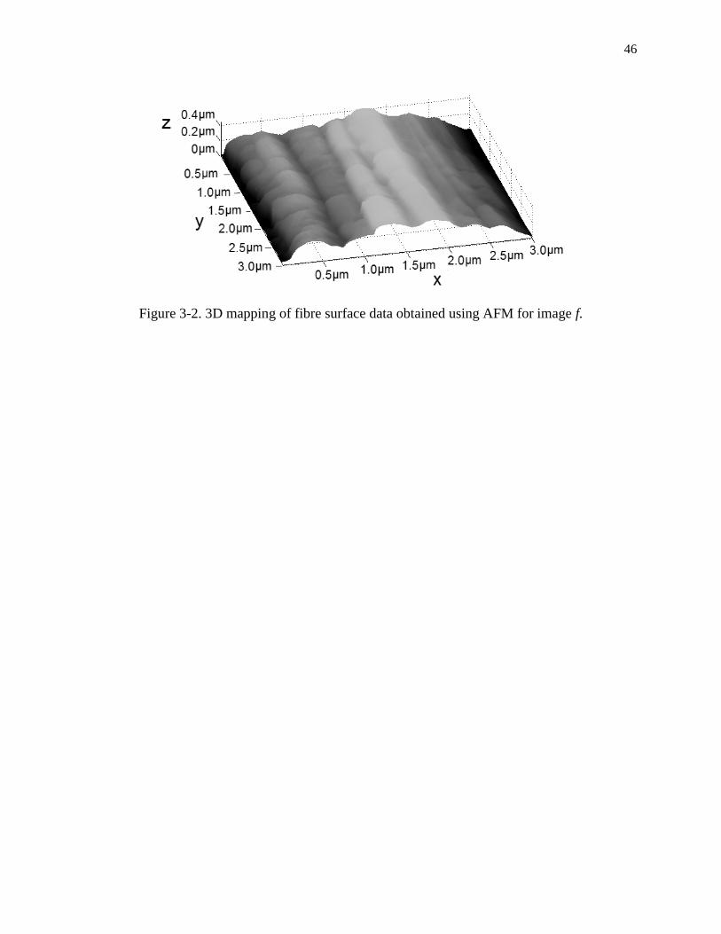
46

Figure 3-2. 3D mapping of fibre surface data obtained using AFM for image f.

47

Figure 3-3. Height deviation in the circumferential (a), and longitudinal (b) directions for AFM

image a.

a) b)

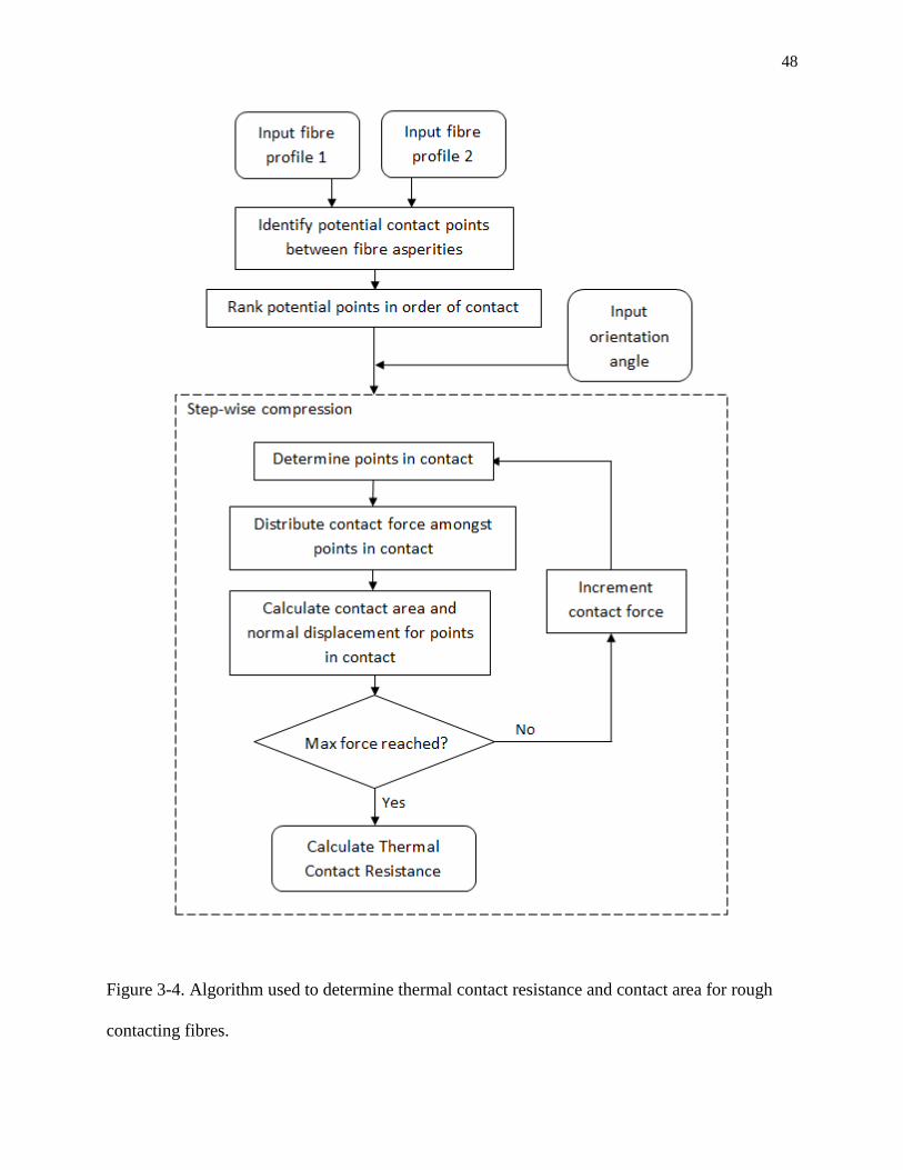
48

Figure 3-4. Algorithm used to determine thermal contact resistance and contact area for rough

contacting fibres.

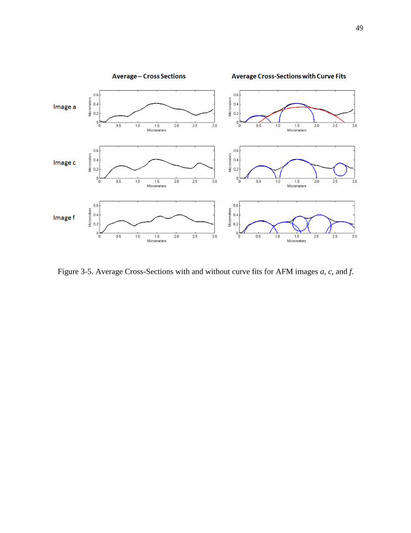
49

Figure 3-5. Average Cross-Sections with and without curve fits for AFM images a, c, and f.

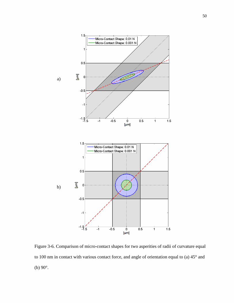
50

a)

b)

Figure 3-6. Comparison of micro-contact shapes for two asperities of radii of curvature equal

to 100 nm in contact with various contact force, and angle of orientation equal to (a) 45° and

(b) 90°.

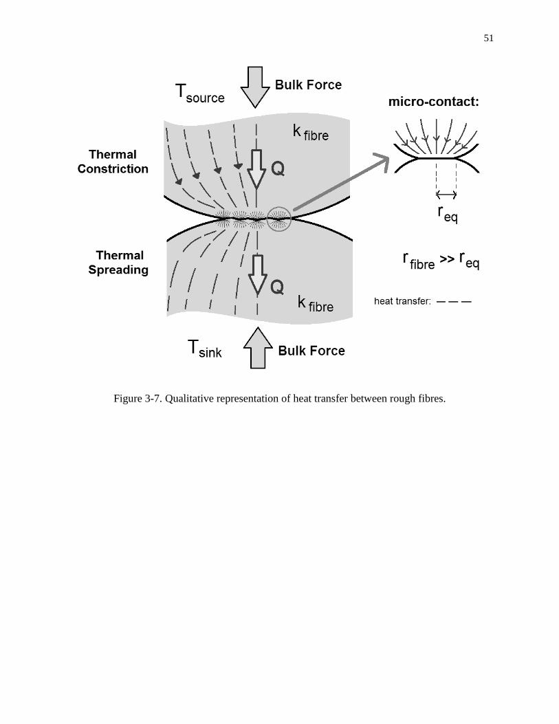
51

Figure 3-7. Qualitative representation of heat transfer between rough fibres.

52

Figure 3-8. Micro-contact area versus contact force for two AFM image a type profiles in

contact, for an angle of orientation of (a) 30°, (b) 45°, and (c) 90°.

a)

b)

c)

53

Figure 3-9. Total Contact Area versus Contact Force for Rough and Smooth Cases

.

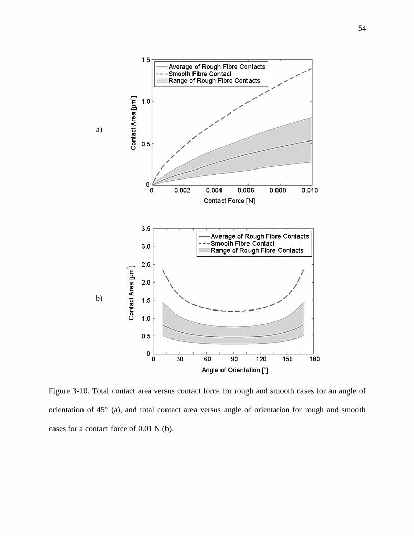
54

a)

b)

Figure 3-10. Total contact area versus contact force for rough and smooth cases for an angle of

orientation of 45° (a), and total contact area versus angle of orientation for rough and smooth

cases for a contact force of 0.01 N (b).

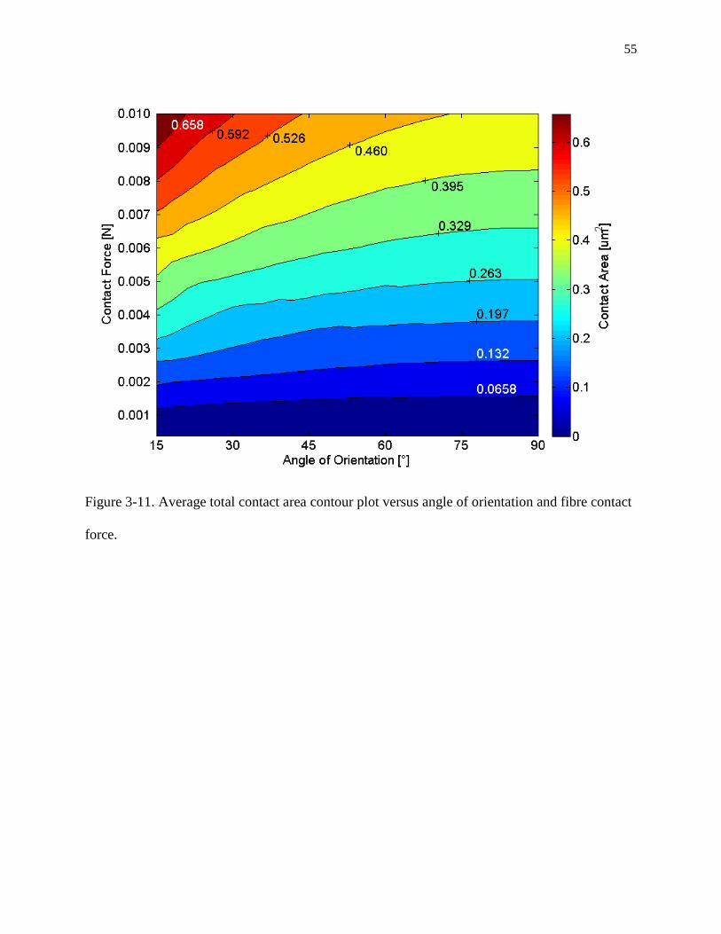
55

Figure 3-11. Average total contact area contour plot versus angle of orientation and fibre contact

force.

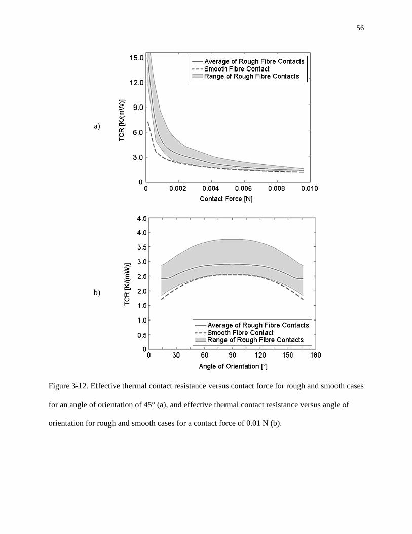
56

a)

b)

Figure 3-12. Effective thermal contact resistance versus contact force for rough and smooth cases

for an angle of orientation of 45° (a), and effective thermal contact resistance versus angle of

orientation for rough and smooth cases for a contact force of 0.01 N (b).

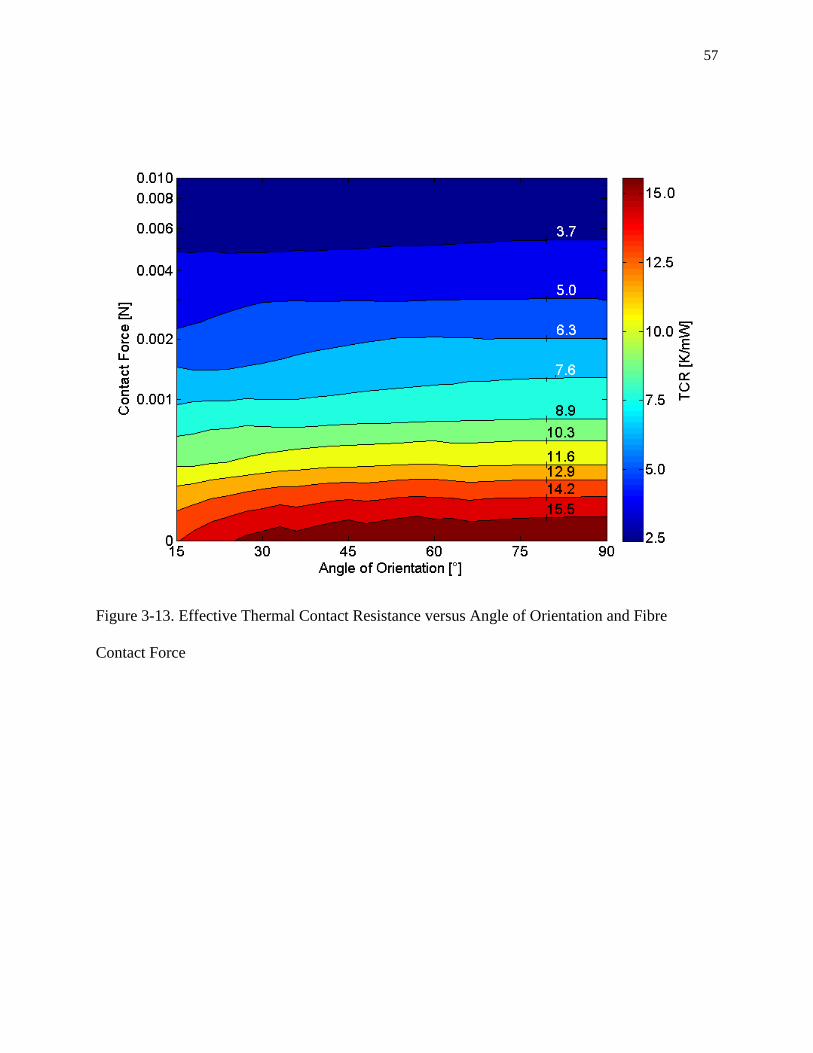
57

Figure 3-13. Effective Thermal Contact Resistance versus Angle of Orientation and Fibre

Contact Force

58

Chapter 4: Characterization of the MPL

4.1 Introduction

In this chapter, atomic force microscopy (AFM) and scanning electron microscopy (SEM)

images of two commercially available MPL materials; SGL-10BB and SGL-10BC, are analyzed

for the purpose of determining the impact of nano-scale features on effective thermal

conductivity modeling. Particle diameters and the nature of particle contacts were characterized

and presented as inputs for future stochastic MPL models. The need for both high-resolution

MPL reconstructions and material-specific data regarding MPL nano-features in heat transfer

modeling is highlighted in this chapter. Also, a robust model based on the Gauss-Seidel iterative

method is presented as a useful technique for analyzing the effective thermal conductivity of

multi-phase MPL structures. The results of this study have been presented for the first time in the

literature, in the recently submitted journal manuscript [61].

4.2 Motivation and Objective

The MPL is a critical component to the PEM fuel cell that has been shown to enhance cell

performance by reducing flooding at the interface between the catalyst layer (CL) and GDL [28],

thereby increasing catalyst utilization efficiency for electrochemical energy conversion [34].

Also, the addition of the MPL has been found to decrease water saturation in the cathode of the

PEM fuel cell, which improves the ability for inlet gases to reach the reaction site [62] due to its

highly hydrophobic nature [8]. However, due to its high polytetrafluorethylene (PTFE) content,

incorporation of an MPL tends to lower the overall effective thermal conductivity of the

diffusion media [8]. Therefore, there is a growing interest in optimizing the design of the MPL

59

structure via computational modeling [21,34] with respect to both water and thermal energy

management, even though the batch-to-batch variations and length scale of the MPL features

contribute to the challenge of validating numerical models [22].

The MPL structure is a relatively new component in the PEM fuel cell. Effective thermal

conductivity models are evolving to more accurately model the material structure. For example,

for the case of modeling the GDL, initial effective thermal conductivity models assumed fibres

were straight and smooth [5,7,9,20,25,26], however recent studies have found that higher

resolution features of the GDL fibres, such as the fibre roughness [47] and waviness [45], should

be considered. In previous literature [21,22,34], the nano-features of the MPL (i.e. nature of

particle-to-particle contacts) were not considered, though they may have a critical impact on rate

of heat transfer in the solid-space. The findings in literature indicate that only the MPL bulk

properties, such as agglomeration shape [21,34], porosity [21,34], thickness [34], and penetration

depth into the GDL [6,34], have been considered. Also, in these models, generic MPL

specifications regarding the particle size and pore-space have been used in the reconstructions,

without consideration of MPL structure variability among material types and manufacturers [22].

The motivation of this chapter is to obtain material-specific structural data on the nano-features

of SGL-10BB and SGL-10BC, including the particle diameter and nature of particle contact,

which will provide fuel cell modelers the reconstruction resolution required to accurately model

heat transfer in the MPL. The Gauss-Seidel iterative method is presented as a robust tool which

can be applied to multi-phase conductive heat transfer modeling. With the findings in this study,

MPL materials can be designed to optimize cell performance with respect to improving the

effective thermal conductivity [44].

60

4.3 Characterization of MPL Materials

As can be seen from the SEM image shown in figure 4-1, the MPL is comprised of particles of

various sizes. This is well documented within the literature regarding the MPL, however no data

has been published on the quantification of the MPL particle size distribution (to the best of the

authors’ knowledge). In order to determine the particle size distribution within the MPL,

information regarding the curvature of the particles is required. AFM functioning in tapping

mode was used to obtain surface information for both SGL-10BB and SGL-10BC. Seven

samples of both materials were imaged with an atomic force microscope (Nanoscope IIIa

Multimode by Digital Instruments and MFP-3D Infinity by Oxford Instruments). For each

sample, images were obtained using a frame size of 1x1 μm2. The region of interest was selected

to obtain a resolution of 2 nm per pixel for measuring the particle curvature (based the expected

particle size [21]). Also, the frame size was based on the results of Wargo et al. [63], where it

was found that the representative elementary volume of the MPL based on diffusivity

calculations is 1 µm3. An example of the AFM results is shown in figure 4-2.

The results obtained from AFM provide the resolution required to analyze the radii of curvature

of the particles, from which the particle size distributions could be obtained. The particle centre

coordinates (x- and y-positions) were located by determining the local maxima within the

respective AFM binary images. The particles were assumed to be spherical. The centres of

adjacent particles, with x- and y-coordinates equal to those of the local maxima, were connected

with straight lines, from which the surface height information of the particles was obtained

(along the directions connecting the particle centres). The surface height information for over

400 particles was analyzed using the AFM images of SGL-10BB and SGL-10BC.

61

A smoothing filter was applied to the surface height contours of connecting particles in order to

reduce the noise attributed to the AFM measurement (figure 4-3 shows an example). The

smoothing filter was applied in MATLAB using the locally weighted scatter plot smooth or loess

function, which uses a locally weighted linear regression model to filter the data. A span of 30%,

corresponding to the percentage of data points near the data point considered (included in the

curve fit calculation), was used reduce the noise attributed to the AFM measurement. Circles

were fitted to the curved regions based on the Taubin method [64] in order to find particle

diameters and filling radii of particle-particle contacts. An example is shown in figure 4-4, where

the curved black line represents the filtered AFM data. I define the particle diameters as the

diameter of the circles fitted to the protruding regions of the filtered AFM data. The location of

the protruding region was set to the location near the local maxima where the concavity1 is

negative (concave down). The filling radius is defined as the radius of a circle which fits the

concave up (positive concavity) regions of the filtered AFM data, forming a particle

connection. The particle protrusion and particle connection regions are shown schematically in

figure 4-3.

The particle size distributions and filling radius distributions from the 2D height contours are

presented in figures 4-5 and 4-6, where the solid line represents gamma-distribution curve

fittings. The particle diameter and filling radius distributions for both SGL-10BB and SGL-10BC

can be compared in figure 4-7. Table 1 includes the shape parameter and scale parameter, which

can be used to reproduce the statistical distributions that can be used as inputs into future

stochastic models. As can be seen in figures 4-5 and 4-6, there is a wide range of particle

1 Concavity is mathematically defined as the second derivative of the height ( ( )),

where ( ) is concave up at if ( ) , ( ) is concave down at if ( ) , and ( ( ))

is an inflection point if ( ) .

62

diameters and filling radii for both materials. In SGL-10BC, there are large particle sizes as

measured with AFM yielding an average particle size of 60.9 nm, compared to 38.4 nm for

SGL-10BB (table 1). Although the particle size distributions measured is larger than that

documented by Becker in [21,34], the mean particle diameter (for SGL-10BB only) and filling

radius agree well with those documented by Becker in [34]. Therefore, the MPL nano-structures

are material dependent [22]. Particle size and filling radius distributions can also be obtained for

other types of diffusion media, characterizing their material-specific structural properties as well.

4.4 Thermal Model

MPL particle structures were generated computationally to reflect the impact of the nature of

contact between particles on thermal conduction. The types of structures considered vary the

nature of contact between particles, and are shown schematically in figures 4-8 and 4-9. The

parameters controlling structural features are discussed in detail in section 4.5. The method used

for determining the effective thermal conductivity of various particle contact structures is based

on the Gauss-Seidel iterative method. The main mode of heat transfer is conduction between

MPL contacts [21,34], since the pores of the MPL are small, and the fluid velocity is low

(negligible convection) [58]. Heat transfer via radiation is assumed to be negligible [65] since the

operating temperature of the PEM fuel cell is 80°C [5,20]. Therefore the heat transfer between

MPL particle structures is modeled as purely conductive in this thesis.

4.4.1 Thermal Model Description

Heat transfer within the MPL particle structures is modeled by discretizing the structures into

cubic elements, from with the Gauss-Seidel iterative method (based on Fourier’s law of

conduction) is applied. A schematic of a MPL particle structure (not showing the cubic elements

63

which form it) is included in figure 4-8a, while figure 4-8b includes a single cubic element taken

from the structure and its neighbours. Constant temperature boundary conditions were positioned

at the top and bottom faces of the modeled MPL particle structure, denoted and . A

linear temperature gradient from the bottom to the top surface was used initially for the

intermediate elements in both cases. The element temperatures are calculated and updated until

the bottom and top heat fluxes are within 0.1% of each other, which is assumed to simulate

steady state conditions and calculation convergence. For the MPL particle structures analyzed in

this chapter, insulated boundary conditions were imposed on the four side walls.

The structure analyzed is discretized into cubic elements. Each element has an energy balance

comprised of six terms, representing the heat transfer across the different faces of the element

(up [U], down [D], north [N], south [S], east [E], and west [W]). Each structure was treated as a

two-phase material with a solid-phase and fluid/matrix-phase. The matrix-phases considered

were stagnant air with thermal properties equivalent to air at 80°C (operating temperature of

PEM fuel cells) [58], representing unsaturated MPL, and liquid water at 80oC, representing

saturated regions in the MPL. Equations 4.1-4.3 represent the approach to determining the

temperature profile of the structure under consideration, where an individual element

temperature is denoted by .

( )

Each of the respective heat transfer rates, between the 6 directions shown in equation 4.1, can be

calculated using equation 4.2, where represents heat transfer between the element under

consideration and neighbouring element i (U, D, N, E, S, W), is the voxel width (detailed

discussion in section 5.5.2), is equal to , and is the temperature of element i.

64

( )

( )

The conductivity of the considered and neighbouring elements would affect the heat transfer

rate: . An effective thermal conductivity between neighbouring voxels, , defined in

equation 4.3, is therefore used in the analysis.

( )

( )( )

⁄

In equation 4.3, represents the thermal conductivity of the element under consideration,

while is the thermal conductivity of the neighbouring element. The thermal conductivity of air

as the fluid-phase is 0.03 Wm-1

K-1

[25], while the thermal conductivity of liquid water was

modeled at 0.58 Wm-1

K-1

[25]. The thermal conductivity of the solid material ( ) however

depends on the PTFE content of the MPL considered, which is well dispersed throughout the

MPL solid-phase; in agreement with the findings of Nanjundappaa in [22]. Therefore, the

thermal conductivity for the solid-phase was calculated using equation 4.4, where is the

thermal conductivity of carbon (120 Wm-1

K-1

), is the thermal conductivity of PTFE

(0.649 Wm-1

K-1

) [25], and is the volume percentage of PTFE used (5% for both

materials). The thermal conductivity for the solid-phase of SGL-10BB and SGL-10BC was

determined to be 114 Wm-1

K-1

.

( ) ( )

Once the temperature profile of the structure (calculated using equations 4.1 to 4.4) has

converged, the effective thermal conductivity of the structure ( ) can be determined using

equation 4.5, where is the conductive heat transfer in the direction of the initial temperature

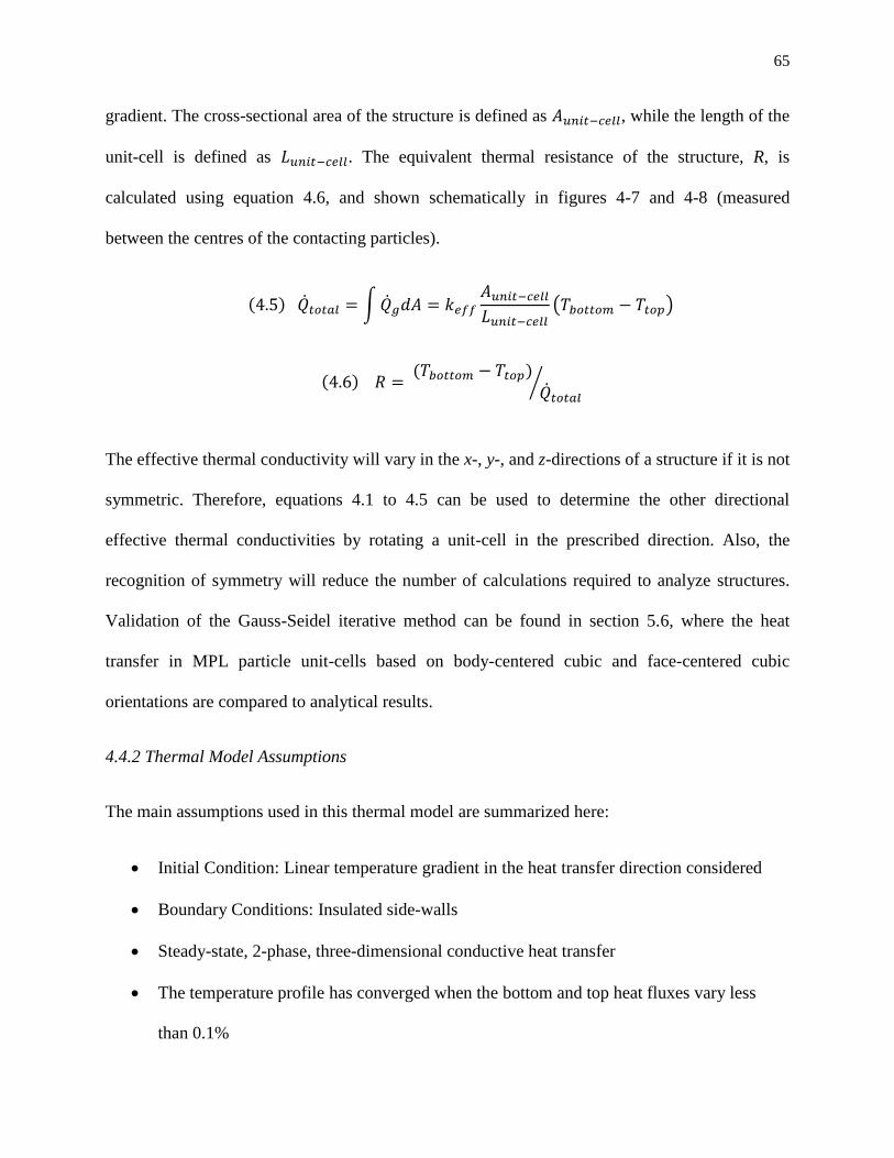
65

gradient. The cross-sectional area of the structure is defined as , while the length of the

unit-cell is defined as . The equivalent thermal resistance of the structure, R, is

calculated using equation 4.6, and shown schematically in figures 4-7 and 4-8 (measured

between the centres of the contacting particles).

( ) ∫

( )

( ) ( )

⁄

The effective thermal conductivity will vary in the x-, y-, and z-directions of a structure if it is not

symmetric. Therefore, equations 4.1 to 4.5 can be used to determine the other directional

effective thermal conductivities by rotating a unit-cell in the prescribed direction. Also, the

recognition of symmetry will reduce the number of calculations required to analyze structures.

Validation of the Gauss-Seidel iterative method can be found in section 5.6, where the heat

transfer in MPL particle unit-cells based on body-centered cubic and face-centered cubic

orientations are compared to analytical results.

4.4.2 Thermal Model Assumptions

The main assumptions used in this thermal model are summarized here:

Initial Condition: Linear temperature gradient in the heat transfer direction considered

Boundary Conditions: Insulated side-walls

Steady-state, 2-phase, three-dimensional conductive heat transfer

The temperature profile has converged when the bottom and top heat fluxes vary less

than 0.1%

66

Convective heat transfer is minimal since fluid velocity in the pore space is low [58]

Heat transfer by radiation can be assumed to be negligible since the operating

temperature is 80°C [65]

Thermal conductivity of the various phases are constant, and do not change with

temperature

4.5 Thermal Analysis of MPL Particle Contact Types

Figure 4-9 shows schematics of the three particle types: varying overlapping distance between

particles with a filling radius of 0 nm (figure 4-9a), varying filling radius with zero particle

overlap or separation distance (figure 4-9b), and finally, varying separation distance between

particles with a constant filling radius (figure 4-9c). The equivalent thermal resistance of the

particle contacts were determined using the thermal model described in section 4.4. The

particles are assumed to be 50 nm in diameter, approximately equal to the arithmetic average of

the mean particle diameters found in section 4.3. In the particle structure shown in figure 4-9c, a

filling radius equal to 10.8 nm, the mean of the filling radii found in section 4.3, is used. Both

unsaturated (air as the surrounding fluid) and water-saturated (liquid water as the surrounding

fluid) MPL particle contacts were considered. Finally, in figure 4-10, particle structures with

varying particle diameters (and constant filling radius equal to 10.8 nm and separation distance

of 0 nm) are presented. Here one particle is held at a constant diameter (Dia1) of 50 nm, while

the other particle’s diameter (Dia2) varies from 10 nm to 100 nm; within the range of particle

diameters found in section 4.3.

67

4.5.1 Effect of Varying Overlapping Distance on Equivalent Thermal Resistance

The equivalent thermal resistances of overlapping MPL particles were calculated (figures 4-11

and 4-12), and was found to decrease with increasing overlapping distance and found to be

inversely proportional to the contact radius (figure 4-9a). The surrounding fluid thermal

conductivity has a larger impact on the calculated equivalent thermal resistance when the contact

radius is low, since a larger percentage of thermal energy flows through the fluid-phase in this

scenario. Figure 4-11 indicates that the equivalent thermal resistance between particle contacts is

sensitive to the overlapping distance; reducing to half when the overlap distance increase to 4 nm

from point contact, and decreases at a rate of approximately 75 K(mW)-1

per nm when the

overlapping distance increases from 4 nm to 12 nm. Therefore, the selection of the overlapping

distance in stochastic models must be treated with care, especially when the overlapping distance

is less than 4 nm.

4.5.2 Effect of Varying Filling Radius on Equivalent Thermal Resistance

Figure 4-13 and figure 4-14 show the impact of varying the filling radius between particle

contacts on equivalent thermal resistance (figure 4-9b) for air and water as the surrounding

fluids. The equivalent thermal resistance between particles decreases with increasing filling

radius and contact radius, though the change in equivalent thermal resistance tends to plateau

when the filling radius reaches 10 nm. The equivalent thermal resistance decreases by 16% when

the filling radius changes from 10 nm to 25 nm, compared to the 43% decrease in the equivalent

thermal resistance when increasing the filling radius from 1 nm to 10 nm. Therefore, in

stochastic MPL models based on experimentally observed data, the selection of a filling radius is

68

significant when less than 10 nm, and high resolutions should be incorporated into modeling of

the MPL particle connections in order to incorporate this effect.

4.5.3 Effect of Varying Separation Distance on Equivalent Thermal Resistance

Figure 4-15 includes the effect of altering the separation distance (figure 4-9c) on the equivalent

thermal resistance between MPL particle contacts with a constant filling radius of 10.8 nm. The

equivalent thermal resistance increases exponentially with separation distance while being

sensitive to the fluid-phase thermal conductivity (figure 4-16). The separation distance is a key

parameter required to analyze the heat transfer between particle contacts in the MPL due to its

extreme impact on the equivalent thermal resistance. Based on these insights, the predictive

model development would benefit from quantifying the particle separation distance in MPL

materials. This information can only be obtained using data from a 3-dimensional reconstruction

of the MPL materials with nano-resolution.

4.5.4 Effect of Varying Particle Diameter Ratio on Equivalent Thermal Resistance

The effect of varying the particle diameters (for two connected particles) on the equivalent

thermal resistance is presented in figure 4-17. A separation distance of 0 nm and a filling radius

of 10.8 nm were used in this study. Here the particle diameter ratio (Dia1/Dia2) is shown

schematically in figure 4-10, where Dia1 is changed from 10 nm to 100 nm. As Dia1/Dia2

increases, the contact area between the particles increases, causing the equivalent thermal

resistance to decrease. The equivalent thermal resistance is sensitive to the Dia1/Dia2 when

Dia1/Dia2 < 1, and less sensitive for Dia1/Dia2 > 1.

Using the shape parameters and scale parameters (table 4-1), 10,000 particle pairs representing

fictitious particle connections were randomly generated while holding one particle diameter

69

constant at 38.4 nm (SGL-10BB) or 60.9 nm (SGL-10BC) respectively (material averages). The

particle diameter ratios were then computed and summarized in figure 4-18. The average

particle diameter ratio for SGL-10BB and SGL-10BC is less than 1. Therefore, assuming 10,000

particle connections is sufficient and considering the results of figure 4-18, it was found that the

MPL should not be modeled with constant particle size. However, it is important to note that this

analysis has been based on studies involving two particles in contact, and should be extended to

multiple particles in contact. Stochastic models should be computed using variable particle sizes

to explore the impact on MPL effective thermal conductivity modeling, as the minimum particle

size used in the reconstruction will gauge the level of resolution required to accurately model the

MPL structure.

The analysis in section 4.5 compares various MPL particle structures and the impact of structural

features on the equivalent thermal resistance. Section 4.5 should be used as a tool for future MPL

models, helping justify the assumptions used in the construction of the particle-based

agglomerations found in the MPL.

4.6 Conclusions

In this study, nano-features of MPL structure were analyzed, and the impact of incorporating

those features into equivalent thermal resistance calculations was investigated. It was found that

the particle diameters in SGL-10BB are smaller than those in SGL-10BC, having mean

diameters of 38.4 nm and 60.9 nm respectively, reflecting variability among material types. The

separation and overlapping distance between MPL particles had the largest impact on equivalent

thermal resistance. For example, the equivalent thermal resistance between MPL particles was

found to decrease by half when the overlapping distance increased to 4 nm from point contact,

70

while the equivalent thermal resistance increases exponentially with separation distance. Also,

the equivalent thermal resistance between MPL particles is sensitive to the filling radius for

values less 10 nm and particle diameter ratios less than 1. If these parameters, such as the particle

spacing or the filling radius, can be controlled in the fabrication of new MPLs, the effective

thermal conductivity can be greatly increased. Also, by incorporating material-specific

nano-features in MPL computational reconstructions, the thermal gradients within the MPL can

be computed more accurately, and the effective thermal conductivity of the MPL, which has

been found to depend on the MPL particle contact [22], can be accurately computed. The results

found here are useful inputs to existing and future MPL models, driving them towards more

realistic reconstructions of the MPL. The results of this study can assist in the fabrication of

better, advanced materials, further improving the efficiency of the technology, driving it towards

global commercialization.

71

4.7 Tables

Table 4-1. Statistical information based on the gamma probability distribution regarding MPL

particle contacts and particle connections

Particle Diameter Filling Radius

SGL-10BB SGL-10BC SGL-10BB SGL-10BC

Mean 38.4 nm 60.9 nm 10.1 nm 11.5 nm

Scale Parameter 10.9 19.5 3.0 2.7

Shape Parameter 3.5 3.1 3.3 4.2

72

4.8 Figures

Figure 4-1. SEM image of SGL-10BC showing variance in particle sizes

73

a)

b)

Figure 4-2 AFM images of SGL-10BB MPL with frame size of 1x1 μm2; Figure 4-2a) 3-

dimensional view, Figure 4-2b) Topological view.

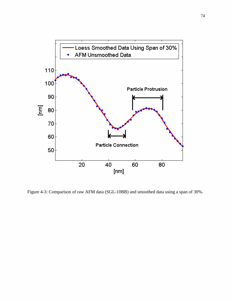
74

Figure 4-3: Comparison of raw AFM data (SGL-10BB) and smoothed data using a span of 30%.

75

Figure 4-4. SGL-10BB particles (red) and particle connections (blue) circle fitted to the

smoothened AFM image height data (black).

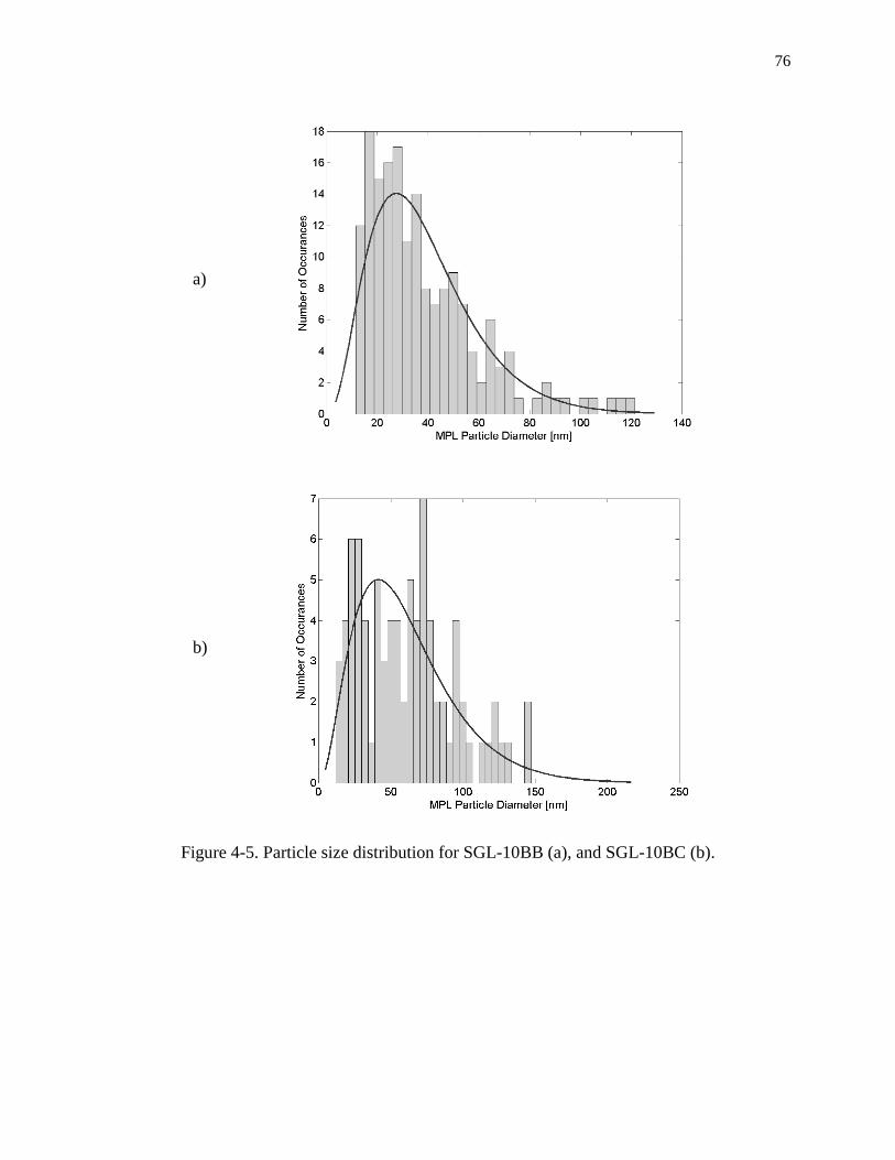
76

a)

b)

Figure 4-5. Particle size distribution for SGL-10BB (a), and SGL-10BC (b).

77

a)

b)

Figure 4-6. Filling radius distribution for SGL-10BB (a), and SGL-10BC (b).

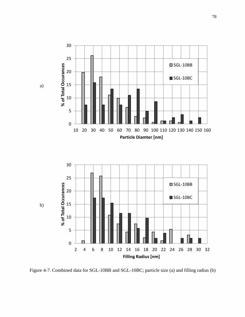
78

a)

b)

Figure 4-7. Combined data for SGL-10BB and SGL-10BC; particle size (a) and filling radius (b)

0

5

10

15

20

25

30

10 20 30 40 50 60 70 80 90 100 110 120 130 140 150 160

% o

f To

tal O

ccu

ran

ces

Particle Diamter [nm]

SGL-10BB

SGL-10BC

0

5

10

15

20

25

30

2 4 6 8 10 12 14 16 18 20 22 24 26 28 30 32

% o

f To

tal O

ccu

ran

ces

Filling Radius [nm]

SGL-10BB

SGL-10BC

79

a)

b)

Figure 4-8. Schematic of MPL particle structure (a) boundary conditions and (b) cubic element

80

Schematic Example 3-D

Reconstruction

a)

b)

c)

Figure 4-9. Schematic of MPL particle contact types; (a) various overlapping distance with no

filling radius, (b) various filling radius with no overlapping or separation distance, and (c)

various separation distance with constant filling radius.

81

a)

b)

Diameter1 = 20 nm

Diameter2 = 50 nm

Diameter1 = 80 nm

Diameter2 = 50 nm

Figure 4-10. Schematic (a) and 3D representation (b) of particles with varying diameter in

contact. Figure 4-10b shows examples for two Dia1/Dia2: 0.4 and 1.6.

82

Figure 4-11. Equivalent thermal resistance between MPL particle contacts versus overlapping

distance.

83

Figure 4-12. Comparison of equivalent thermal resistance with air and water as the surrounding

fluid, versus overlapping distance.

84

Figure 4-13. Equivalent thermal resistance between MPL particle contacts versus filling radius.

85

Figure 4-14. Comparison of equivalent thermal resistance with air and water as the surrounding

fluid, versus filling radius.

86

Figure 4-15. Equivalent thermal resistance between MPL particle contacts versus separation

distance.

87

Figure 4-16. Comparison of equivalent thermal resistance with air and water as the surrounding

fluid as a function of particle separation distance.

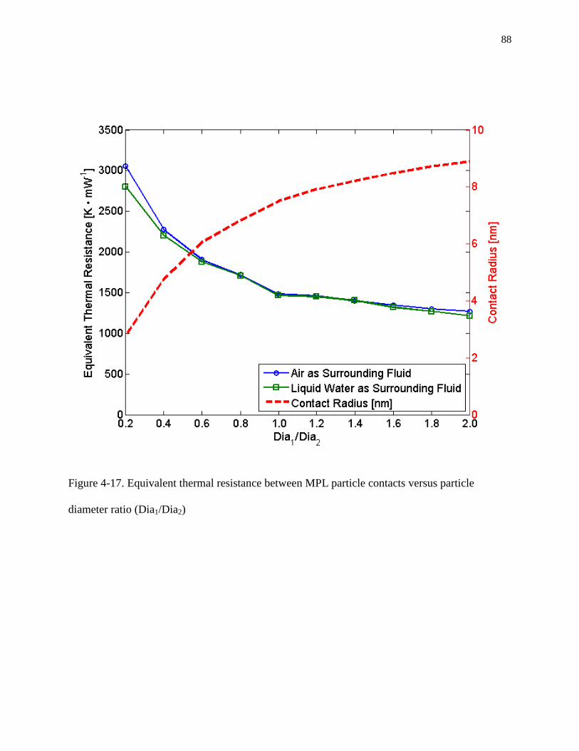
88

Figure 4-17. Equivalent thermal resistance between MPL particle contacts versus particle

diameter ratio (Dia1/Dia2)

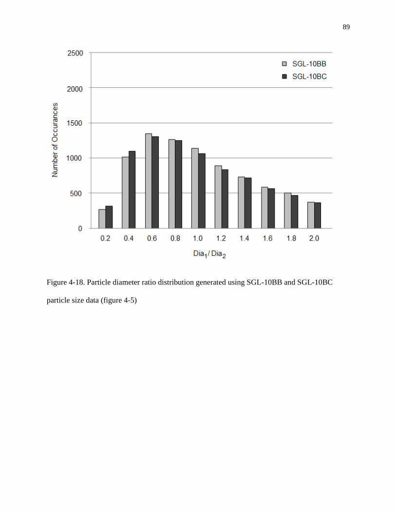
89

Figure 4-18. Particle diameter ratio distribution generated using SGL-10BB and SGL-10BC

particle size data (figure 4-5)

90

Chapter 5: Unit-Cell Analysis

5.1 Introduction

In this chapter, I present the preliminary stages of utilizing unit-cell analysis (UCA) as a

technique for modeling the MPL particle interactions and agglomeration shapes, for the purpose

of modeling the MPL effective thermal conductivity. Various unit-cell structures are constructed

using the particle diameter and filling radius distributions of SGL-10BB and SGL-10BC

(chapter 4) and are analyzed for their effective thermal conductivity, to be used as building

blocks for constructing stochastic or deterministic MPL materials.

5.2 Motivation and Objective

Due to the random nature of the MPL particle agglomerations [66], the variability in the MPL

structure [22], and scale of the structural features [21,67], it is difficult to develop an accurate

representation of the MPL to measure the effective thermal conductivity. In particular, the

resolution required to effectively model the contact region between particles has not been

achieved in literature for modeling the solid-space of the MPL [67,68]. Based on the particle

diameter and filling radius distributions for SGL-10BB and SGL-10BC (chapter 4), the MPL

should be modeled with material-specific inputs regarding the particle size and nature of contact.

The current models found in literature are based on the stochastic reconstruction of the entire

MPL material [21,34] or deterministic reconstructions of the MPL based on computed

tomography [22,67,68]. Incorporating higher resolution information is necessary for modeling

heat transfer between MPL particles and nano-pores found between the particles [22]

(as discussed in section 4.5), but has been disregarded in the past since the resolution of

91

computed tomography reconstructions of the MPL are incapable of imaging the nano-structures

with such detail [67].

UCA has been used to model the GDL by Sadeghi et al. [7,9,26] who considered fibre

interactions to be repeating structures. To the best of the author’s knowledge, the results of this

chapter highlight the first time UCA has been used to analyze the effective thermal conductivity

of the MPL. Therefore, UCA is presented as a novel technique for analyzing the MPL under the

necessary resolution for modeling nano-features in the structure, and provides the ability to

parameterize those nano-structural features with respect to effective thermal conductivity

calculations, helping further optimize the MPL structure. UCA is based on having MPL

modeling being approached into two length scales; nano-scale for particle interactions and

agglomerations (via unit-cells), and micro-scale for the modeling of cracks and large pore spaces

(not covered in this chapter). Therefore the objective of this study is to obtain unit-cells for

SGL-10BB and SGL-10BC that can be used as building blocks to reconstruct the MPL

stochastically, or to populate low-resolution material reconstructions which may have been

previously viewed as insufficient for modeling heat transfer. A schematic of how UCA can be

applied in the construction of nano-resolved MPL structures is shown in figure 5-1

(in 2-dimensions for visualization purposes).

5.3 Unit-Cell Reconstructions of MPL Particles

The unit-cell reconstructions utilized to model MPL particles are based on body-centred cubic

(BCC) and face-centred cubic (FCC) orientations. The BCC unit-cell contains particles

positioned at the volumetric centre of the unit-cell, and eight corners. The FCC unit-cell is

similar to the BCC structure, with eight 1/8th

particles located at the eight corners of the unit-cell,

92

however, instead of having a particle at the volumetric centre, six half-particles are centred at the

six faces of the unit-cell. Visual representations of BCC and FCC structures, assuming point

contact, are displayed in figure 5-2, for various unit-cell side lengths, a, measured in voxels.

Increasing the voxel resolution (side-length of individual voxels [nm/voxel]) used in the unit-cell

reconstruction improves the accuracy of the reconstruction (section 5.3.1) and the accuracy of

the measured effective thermal conductivity (section 5.3.2).

5.3.1 Voxel Resolution Selection Based On Unit-Cell Reconstruction Accuracy

One of the first considerations in the development of the unit-cells is the resolution used,

corresponding to the number of voxels utilized in the reconstruction. As can be seen in

figure 5-2, as voxel count increases, related to a, the particles appear to be more spherical. The

accuracy of the reconstruction can be quantified by using the solid volume fraction, svf, which is

defined as the amount of solid volume in a unit-cell divided by the total unit-cell volume.

Equations 5.1 and 5.2 include the actual solid volume fractions for the BCC and FCC structures,

assuming the particle diameters are all equal. The unit-cell side length, a, can be measured in

terms of the particle radius, r, given that the particles are touching along the body-diagonal for

BCC structures ( √ ), and along the face-diagonal for FCC structures ( √ ).

( ) (

) (

) √

( ) (

) (

) √

Table 5-1 shows the svf of the various reconstructions analyzed in figure 5-2 to determine the

effect of varying the voxel resolution on the reconstruction accuracy. As the total number of

93

voxels used in the reconstruction increases, the svf of the unit-cell approaches the actual svf

values of 0.68 for BCC and 0.74 for FCC.

5.3.2 Voxel Resolution Selection Based On Effective Thermal Conductivity Measurement

Though increasing the voxel count in the unit-cell reconstruction causes the svfs to approach the

analytical values, it is also important to understand the impact of voxel count on the measured

effective thermal conductivity ( ). Figure 5-3 shows the impact of increasing the unit-cell

voxel count from 513 to 101

3 (corresponding to an increase in voxel resolution) for BCC and

FCC unit-cell reconstructions on the numerically calculated . Figure 5-3 uses the thermal

model described in section 4.4 to solve for the , with a solid thermal conductivity ( ) to

matrix-phase thermal conductivity ( ) ratio equal to 1000. The numerical data is

compared with analytical results conducted by Lord Rayleigh and McPhedran et al. [69,70],

which are discussed in detail in section 5.5: Validation of the Thermal Model presented in

Section 4.4.

As can be seen in figure 5-2, increasing the voxel count not only improved the reconstruction

accuracy, but also improved the accuracy of the measurement, showing an average increase

in accuracy (compared to the analytical data) of 34% for BCC structures, and 24% for FCC

structures. However, it is important to note that the time required for the analysis of the unit-cells

increased by approximately 161 times (since the number of computations increased). Therefore

although an increase in voxel count from 513 to 101

3 is justified by the increase in accuracy, a

further increase in accuracy, such as from 1013 to 501

3 is not justified (since the results for 101

3

are already quite accurate). Nonetheless, a voxel count of 1013 voxels per unit-cell was used in

94

all of the reconstructions (including those in section 4.4) with the assumption that the accuracy of

the results in figure 5-3 and section 5.6 are sufficient for this study.

5.3.3 Irregular Unit-Cells

In order to form particle agglomerations using unit-cells, BCC and FCC structures with some

missing components must also be included. These types of unit-cells are described herein as

irregular unit-cells. For the BCC and FCC structures, there can be numerous combinations of

removing selected particles from the structures, resulting in many unit-cells. Figure 5-4 and 5-5

represents the distinct cases for BCC and FCC respectively, from which any irregular unit-cell

can be obtained by either rotating or flipping any of these structures. When building

agglomerations from the irregular unit-cells, the boundary conditions of the neighbouring

unit-cells must be compliant. For example, you may have a BCC-Irregular-1 unit-cell beside a

BCC-Irregular-2 unit-cell, provided that the corner diameters for both unit-cells are the same.

BCC unit-cells could be mixed with FCC unit-cells for the special irregular cases where one of

the faces of the FCC unit-cells does not have a face particle. Irregular unit-cells are analyzed

with SGL-10BB and SGL-10BC particle diameter and filling radius inputs from section 4.3, in

section 5.4.3.

5.4 Comparison of MPL Particle Features on Unit-Cell Effective Thermal Conductivity

UCA is presented as a method for modeling the effective thermal conductivity of the solid-space

of SGL-10BB and SGL-10BC, from which material-specific parameters are required for analysis

(results of section 4.3). The effective thermal conductivity of various unit-cell configurations

informed from AFM data is presented here, where the side-walls of the unit-cells are modeled

95

using mirror boundary conditions, simulating the effect of having compliant neighbouring

unit-cells, rather than the insulated side-wall boundary conditions used in chapter 4.

5.4.1 Filled Contact Algorithm

Until this point in chapter 5, only unit-cells with particles forming point contact have been

considered. However, the results of section 4.3 indicate that there is filling volume between

particles found in SGL-10BB and SGL-10BC, with curvature equal to the filling radius. The

method used to fill in the contacts of the generated unit-cell structures is straightforward. A

sphere of radius equal to the filling radius traverses the surface of the particles in the unit-cell,

keeping in contact with the particle surfaces. The sphere is not allowed to overlap any of the

solid-space. The regions that the sphere cannot reach, due to the surfaces of the particles being

too close together, is converted into solid material. The end result is that the contact regions

between particles are filled with solid volume maintaining a curvature equal to the filling radius.

A visual example of this is shown in figure 4-9b and figure 4-9c.

5.4.2 SGL-10BB and SGL-10BC Regular Unit-Cells

The parameters used for the BCC and FCC reconstructions of SGL-10BB and SGL-10BC

unit-cells, in particular the particle diameter and filling radius, are the mean values included in

table 4-1. Since the actual separation/overlapping distance cannot be determined via AFM, the

particle configurations built have been parameterized with two extremes: a separation distance

equal to the filling radius of the material or a separation distance equal to zero. The unit-cell

reconstructions for SGL-10BB, which are similar in shape to SGL-10BC, can be viewed in

figure 5-6 for both separation distances. It is important to note that the images shown here show

the full particles at the unit-cells face boundaries for visualization purposes. The actual modeled

96

unit-cells contain 1/8th

particles at the corners (BCC or FCC), and half-particles at the faces

(FCC).

As mentioned in section 5.3.2, the unit-cells were discretized with a equal to 101 voxels with

equal particle diameters. Based on the characteristic equations for BCC and FCC unit-cells, a

[nm] could be obtained through the use of equations 5.3 and 5.4, for BCC and FCC

configurations respectively, where is the separation distance between particles. The voxel

resolution is defined as a [nm] divided by 101 voxels. Table 5-2 includes the voxel resolution for

the various material-specific unit-cells constructed.

( ) √

( ) √

Using the method described in section 4.4, the SGL-10BB and SGL-10BC BCC and FCC

unit-cells were analyzed for their , assuming the cells were both unsaturated (table 5-3) and

saturated with liquid water (table 5-4). The of the unit-cells vary significantly with the

separation distance; in agreement with the findings from section 4.5.3, highlighting the

sensitivity of the MPL to . Also, the of the unit-cells is dominated by the solid-phase

thermal conductivity, varying little with the fluid-phase thermal conductivity. This is mainly due

to the high solid volume fractions seen for these unit-cell configurations, where the effect of

fluid-phase thermal conductivity will be more significant for irregular unit-cells missing a large

number of particles (figures 5-6 and 5-7). The of the BCC structures are less than that of the

FCC structures, again since there are higher solid volume fractions in FCC and better solid path

connectedness in FCC than in BCC. Finally there are slightly higher values in SGL-10BB

97

compared to SGL-10BC [6], with an average of 5% higher effective thermal conductivity in

SGL-10BB than in SGL-10BC for BCC, and an average of 0.6% higher effective thermal

conductivity in SGL-10BB than in SGL-10BC for FCC. This result is affected by the variance in

the structures which are dictated by the particle diameters and filling radii, forming a larger

particle contact area to particle diameter ratio in SGL-10BB than in SGL-10BC, which causes

SGL-10BB to conduct heat better than SGL-10BC within the unit-cells.

5.4.3 SGL-10BB and SGL-10BC Irregular Unit-Cells

In order to model the MPL particle agglomerations for SGL-10BB and SGL-10BC materials,

irregular unit-cells based on the material specific nano-features (table 4-1) are required. The

complete irregular unit-cell study should incorporate the following combinations:

SGL-10BB and SGL-10BC nano-features

Water-saturated and unsaturated MPL unit-cells

BCC and FCC configurations

Ten different irregular unit-cells for the BCC configuration and sixteen distinct irregular

unit-cells for the FCC configuration were generated. Each of the irregular unit-cells must be

analyzed in the x-, y-, and z-directions. Also, since the exact separation distance is unknown, the

two extremes analyzed in section 5.4.2 must be used in the two different irregular unit-cell

reconstructions. This constitutes to 624 simulations that must be conducted to fully characterize

the SGL-10BB and SGL-10BC materials (which can be reduced by half if the separation distance

of the MPLs is determined, and computed more efficiently using the notion of symmetry in the

heat transfer analysis). Since, in section 5.4.2, the effective thermal conductivity of SGL-10BB

and SGL-10BC structures do not vary significantly, the effective thermal conductivity of

98

SGL-10BB BCC and FCC structures is presented with air as the fluid-phase thermal conductivity

and particle-to-particle separation distance of 0 nm. It is hypothesized that the effective thermal

conductivity will be affected more greatly by the fluid-phase thermal conductivity for irregular

unit-cells with lower svfs, which will be the focus of future work in this area of research.

5.4.3.1 Irregular Unit-Cell Nomenclature

The irregular unit-cell reconstructions are based on the structures discussed in section 5.3.3, with

material information corresponding to SGL-10BB in table 4-1. The effective thermal

conductivities of unsaturated SGL-10BB BCC and FCC with a separation distance of 0 nm can

be found in tables 5-5 and 5-6, respectively. In order to decipher the x-, y-, and z-directions with

respect to the irregular unit-cells, a naming system has been created. The names of the various

irregular unit-cells can be found in tables 5-5 for BCC and 5-6 for FCC, under the irregular

unit-cell number in the “Name” rows. The names given to the irregular unit-cells can be used in

combination with figure 5-7, which contains labels for the particles in different lattice locations,

to determine the directional effective thermal conductivity. The names in tables 5-5 and 5-6

correspond to the particles not present at the particular lattice locations. For example,

BCC-Irregular-3 contains two missing particles at opposite corners on one face of the unit-cell.

The analogous name for BCC-Irregular-3 is “B4”. Similarly, FCC-Irregular-6 has one face with

no particles positioned, and is therefore named “BDQ24”, corresponding to the four corner and

one face particles missing. This naming system helps us distinguish the x-, y-, and z-directions of

the irregular unit-cells using figure 5-7, which cannot be understood with only figures 5-6 and

5-7, since the images in these figures have been rotated for visualization purposes.

99

5.4.3.2 Irregular Unit-Cell Effective Thermal Conductivity

As can been seen in the data in tables 5-5 and 5-6, as the number of removed particles increases,

the effective thermal conductivity decreases, converging towards the fluid-phase thermal

conductivity, which is 0.03 Wm-1

K-1

for air. A significant decrease in effective thermal

conductivity occurs when there is not solid material connecting opposite faces (in the direction

considered). This is due to the relatively low thermal conductivity of the fluid-phase acting as a

thermal insulator, causing the effective thermal conductivity of the unit-cell to decrease

significantly. This is seen in between FCC-Irregular-5 (BDQ2) and FCC-Irregular-6 (BDQ24)

for example, where the effective thermal conductivity in the y-direction decreases from

4.99 Wm-1

K-1

to 0.19 Wm-1

K-1

, since the opposite faces with normal parallel to the y-direction

are no longer connected with solid material, as the particle in the “4” location is removed

(evolving from FCC-Irregular-5 to FCC-Irregular-6). Similar trends are found for BCC and FCC

structures, when certain lattice locations do not have a particle.

5.5 Validation of the Thermal Model presented in Section 4.4

The thermal model presented in section 4.4 was tested using BCC and FCC structures in point

contact, due to their complicated structures and complex thermal gradient patterns arising during

convergence of the temperature field. The numerical results from such unit-cells were compared

with analytical results presented in [69] by Rayleigh. Rayleigh determined the of BCC and

FCC structures of constant particle diameter. Various svfs were analyzed, with limiting cases for

BCC and FCC being 0.68 and 0.74, as explored in equations 5.1 and 5.2 respectively. In the

mathematical formulations conducted by McPhedran [70], who advanced Rayleigh’s work, the

ratio between the to fluid/matrix-phase thermal conductivity was assumed to be

100

infinite. Figure 5-8 includes a comparison of the numerical results conducted in this study with

the analytical data found in literature, for BCC and FCC structures.

In figure 5-8, the effective thermal conductivity to matrix-phase thermal conductivity ratio is

shown as a function of svf. Two ⁄ values were analyzed. The first ratio used the

thermal conductivity of air at 80°C (0.03 Wm-1

K-1

) as and the of SGL-10BB

(114 Wm-1

K-1

), as calculated with equation 4.4. The second ratio used = 100 Wm-1

K-1

while the was set to be 0.1 Wm-1

K-1

, leading to a ⁄ = 1000. The results

obtained for the two respective ⁄ ratios varied by less than 1% for BCC and less

than 5% for FCC. This is in agreement with a study conducted by Jae Kim et al. [71], who

determined that a ⁄ > 1000 can be viewed as ⁄ = ∞. Jae Kim

conducted a secondary study for non-infinite ⁄ [71]. Included in figure 5-9 are

numerical results for a ⁄ = 100, which can be compared to the study conducted in

[71]. Nonetheless, the results give good agreement with the analytically determined data,

obtained by Rayleigh [69], McPhedran [70] and Jae Kim et al. [71].

5.6 Conclusion

In this chapter, a model capable of analyzing the MPL of the PEM fuel cell was developed,

capable of solving issues regarding reconstruction resolution and computational inefficiencies.

Unit-cell analysis was used to analyze the effect of varying MPL structures, SGL-10BB and

SGL-10BC, in terms of effective thermal conductivity. It was found that the structures of

SGL-10BB are slightly more thermally conductive than SGL-10BC. It was also found that the

fluid-phase effective thermal conductivity is not a major contributor in the effective thermal

conductivity of regularly shaped BCC and FCC unit-cells, due to the high conductivity of the

101

solid-phase. The analysis of irregular unit-cells have been presented, and offers a promising,

novel approach to modeling MPL materials, provided that the particle diameter, filling radius,

and separation distance are known. UCA is a modeling tool that can help in the design of the

MPLs at the nano-scale, from which parameters involved in the fabrication can be altered, in

order to optimize the structure in terms of thermal energy transfer in the MPL, further improving

the efficiency of the technology.

102

5.7 Tables

Table 5-1. Impact of voxel resolution on accuracy of BCC and FCC reconstruction

Unit Cell Width,

a [voxels] 11 51 101 501 Actual

Number of

Voxels 10

3 10

6 10

7 10

8 ∞

svf (BCC) 0.83 0.79 0.71 0.684 0.68

svf (FCC) 0.89 0.86 0.79 0.749 0.74

103

Table 5-2. Voxel resolution for various unit-cell reconstructions

Voxel Resolution [nm/voxel] SGL-10BB SGL-10BC

BCC 0.55 0.84

FCC 0.68 1.00

104

Table 5-3. Effective thermal conductivity of various unit-cell configurations with air at 80

oC as

the fluid-phase

keff [Wm-1

K-1

] ds = filling radius [nm] ds = 0 nm

SGL-10BB SGL-10BC SGL-10BB SGL-10BC

BCC 7.01 6.62 20.34 19.20

FCC 11.09 10.97 26.83 26.72

105

Table 5-4. Effective thermal conductivity of various unit-cell configurations with liquid water as

the fluid-phase

keff [Wm-1

K-1

] ds = filling radius [nm] ds = 0 nm

SGL-10BB SGL-10BC SGL-10BB SGL-10BC

BCC 7.37 6.99 20.52 19.42

FCC 11.32 11.23 26.89 26.76

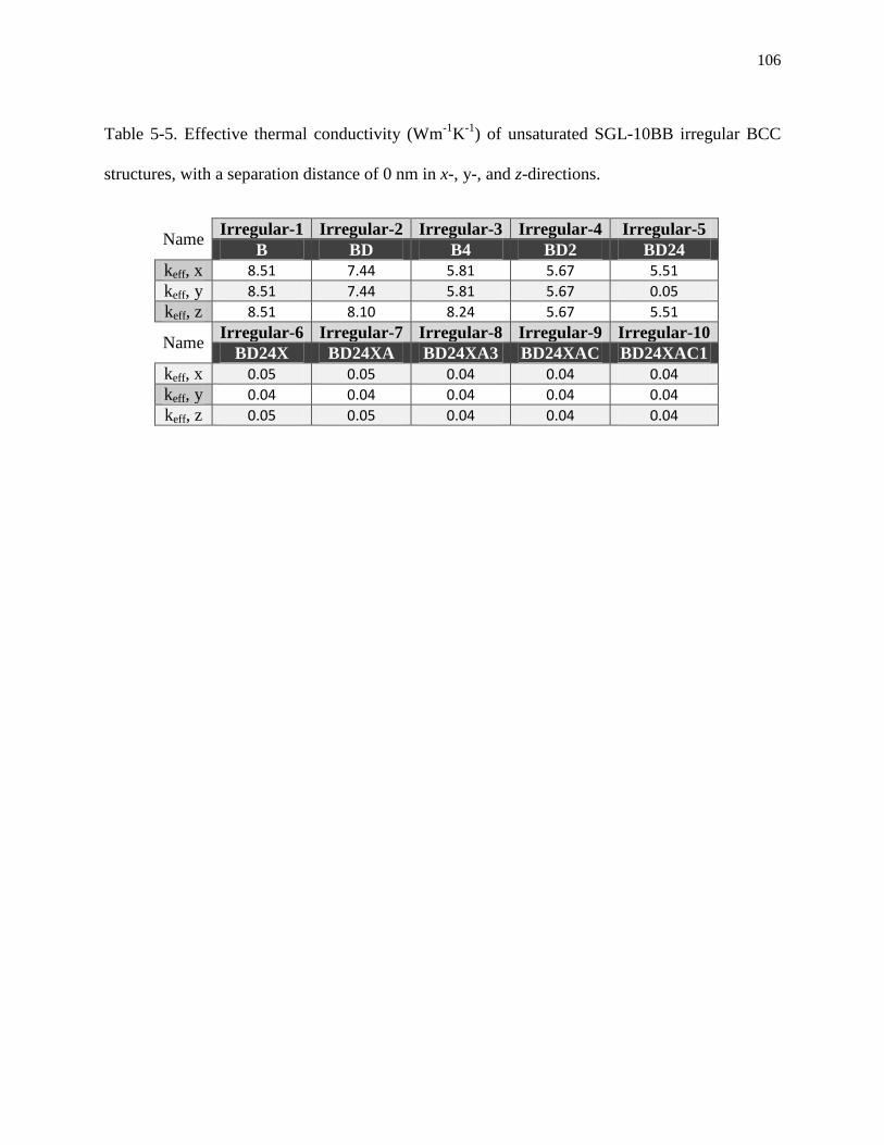
106

Table 5-5. Effective thermal conductivity (Wm

-1K

-1) of unsaturated SGL-10BB irregular BCC

structures, with a separation distance of 0 nm in x-, y-, and z-directions.

Name Irregular-1 Irregular-2 Irregular-3 Irregular-4 Irregular-5

B BD B4 BD2 BD24

keff, x 8.51 7.44 5.81 5.67 5.51

keff, y 8.51 7.44 5.81 5.67 0.05

keff, z 8.51 8.10 8.24 5.67 5.51

Name Irregular-6 Irregular-7 Irregular-8 Irregular-9 Irregular-10

BD24X BD24XA BD24XA3 BD24XAC BD24XAC1

keff, x 0.05 0.05 0.04 0.04 0.04

keff, y 0.04 0.04 0.04 0.04 0.04

keff, z 0.05 0.05 0.04 0.04 0.04

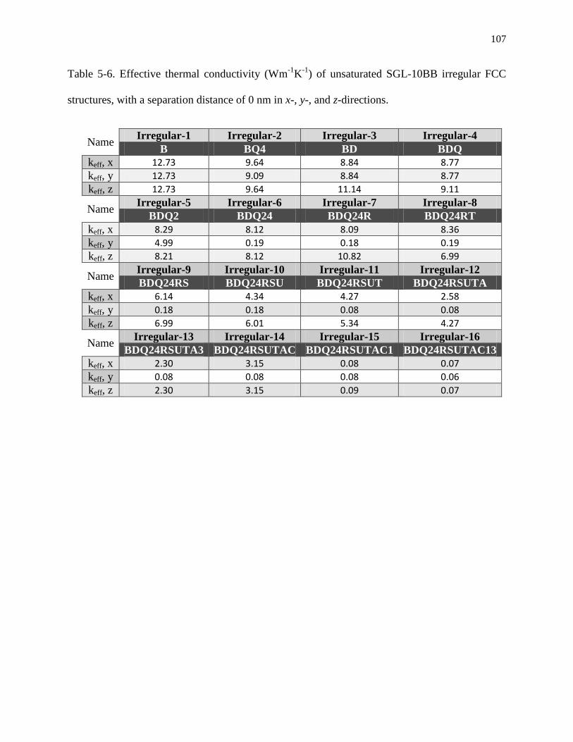
107

Table 5-6. Effective thermal conductivity (Wm-1

K-1

) of unsaturated SGL-10BB irregular FCC

structures, with a separation distance of 0 nm in x-, y-, and z-directions.

Name Irregular-1 Irregular-2 Irregular-3 Irregular-4

B BQ4 BD BDQ

keff, x 12.73 9.64 8.84 8.77

keff, y 12.73 9.09 8.84 8.77

keff, z 12.73 9.64 11.14 9.11

Name Irregular-5 Irregular-6 Irregular-7 Irregular-8

BDQ2 BDQ24 BDQ24R BDQ24RT

keff, x 8.29 8.12 8.09 8.36

keff, y 4.99 0.19 0.18 0.19

keff, z 8.21 8.12 10.82 6.99

Name Irregular-9 Irregular-10 Irregular-11 Irregular-12

BDQ24RS BDQ24RSU BDQ24RSUT BDQ24RSUTA

keff, x 6.14 4.34 4.27 2.58

keff, y 0.18 0.18 0.08 0.08

keff, z 6.99 6.01 5.34 4.27

Name Irregular-13 Irregular-14 Irregular-15 Irregular-16

BDQ24RSUTA3 BDQ24RSUTAC BDQ24RSUTAC1 BDQ24RSUTAC13

keff, x 2.30 3.15 0.08 0.07

keff, y 0.08 0.08 0.08 0.06

keff, z 2.30 3.15 0.09 0.07

108

5.8 Figures

a)

b)

c)

Figure 5-1. Schematic of an MPL cross-section, approximately 1 µm by 1 µm, showing the use of unit-

cells for population low-resolution MPL reconstructions in 2D; (a) schematic of an MPL cross-section,

(b) schematic of a unit-cell populated cross section, and (c) both images overlaid.

109

Figure 5-2. BCC and FCC reconstructions using various number of voxels

a 11 voxels 51 voxels 101 voxels 501voxels

BCC

FCC

110

a)

b)

Figure 5-3. Comparison of voxel count in unit-cell reconstruction with analytical results for

kp/km = 1000 [70], for (a) BCC and (b) FCC structures.

111

BCC-Irregular-1 BCC-Irregular-2 BCC-Irregular-3 BCC-Irregular-4 BCC-Irregular-5

BCC-Irregular-6 BCC-Irregular-7 BCC-Irregular-8 BCC-Irregular-9 BCC-Irregular-10

Figure 5-4. Irregular BCC Lattice Structures

112

FCC-Irregular-1 FCC-Irregular-2 FCC-Irregular-3 FCC-Irregular-4

FCC-Irregular-5 FCC-Irregular-6 FCC-Irregular-7 FCC-Irregular-8

FCC-Irregular-9 FCC-Irregular-10 FCC-Irregular-11 FCC-Irregular-12

FCC-Irregular-13 FCC-Irregular-14 FCC-Irregular-15 FCC-Irregular-16

Figure 5-5. Irregular BCC Lattice Structures

113

a)

b)

c)

d)

Figure 5-6. Various SGL-10BB unit-cell configurations, (a) BCC with ds = 10.1 nm, (b) BCC

with ds = 0 nm, (c) FCC with ds = 10.1 nm, and (d) FCC with ds = 0 nm

114

a)

b)

Figure 5-7. Naming system and co-ordinate axis used to define directional effective thermal

conductivities of irregular BCC (a) and FCC (b) unit-cells.

115

a)

b)

Figure 5-8. Comparison of numerical results with analytical data [69,70], for various

⁄ , (a) BCC and (b) FCC.

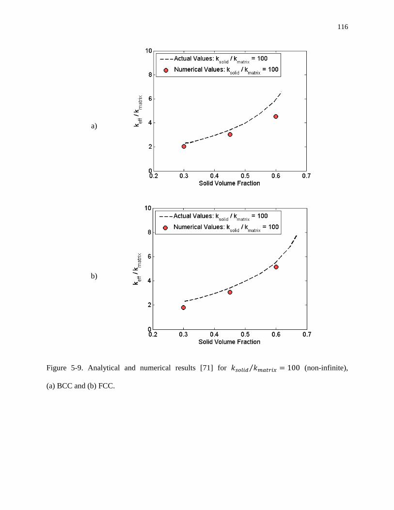
116

a)

b)

Figure 5-9. Analytical and numerical results [71] for ⁄ (non-infinite),

(a) BCC and (b) FCC.

117

Chapter 6: Conclusions

In this thesis, the effect of incorporating high resolution structural features in the MPL and GDL

has been studied to determine the impact on heat transfer modeling in the cathode of the PEM

fuel cell. A literature review regarding the role of the GDL and MPL on thermal energy

management and water management in the PEM fuel cell has been completed. A comprehensive

comparison of literature comparing/contrasting the GDL, MPL, and combined GDL+MPL

substrates (both numerically and experimentally) has been included, highlighting the main

parameters affecting the bulk effective thermal conductivity measurement.

In chapter 3, the impact of fibre surface morphology on the thermal contact resistance between

rough GDL fibres is presented. Carbon fibres housed in untreated Toray GDL were imaged using

AFM to obtain their circumferential roughness. The fibre surface asperities were curve fitted and

applied to an analytical model based on the Greenwood algorithm for rough contact. The thermal

contact resistance between rough contact fibres was calculated using thermal spreading and

constriction resistance equations presented in [57], identifying the validity of the smooth fibre

assumption. In summary:

Rough fibre contact results in smaller contact areas than in smooth fibre contact, with

both rough and smooth fibre contact area increasing with contact force. The contact area

between rough or smooth fibres is minimal when the fibres in contact are orthogonal to

each other.

The thermal contact resistance mean and range decreases with increasing contact force.

The upper bound of the thermal contact resistance range is attributed to rough fibres

118

having asperities with smaller diameters, resulting in smaller micro-contact areas, while

the lower bound corresponds to asperities with larger diameters, resulting in larger

micro-contact areas.

The impact of incorporating fibre surface morphology into thermal contact resistance

modeling is critical when the contact forces between the fibres are low, deeming the

smooth fibre assumption unacceptable for low contact forces. When the contact force is

low, the measured thermal contact resistance is much higher in the rough contact case

than in the smooth contact case. This corresponds to regions under the bipolar plate

channel for example, or any location where there is lower contact force between GDL

fibres.

When the contact forces are high, the rough fibre contact and smooth fibre contact are

similar. For example, when the contact force is 0.01 N, the rough thermal contact

resistance differs from the smooth fibre contact resistance by approximately 10%.

In chapter 4, commercially available MPL materials, SGL-10BB and SGL-10BC, were

characterized with respect to their nano-structures. A curve-fitting algorithm based on the Taubin

method was implemented to measure the curvature of particles, and regions between particles,

corresponding to particle connections. In this chapter, a thermal model based on the

Gauss-Seidel iterative method was also introduced, which has the advantage of modeling the

conductive heat transfer within any multi-phase structure given only the structural data of the

material considered (a direct output from AFM). The Gauss-Seidel iterative method was used to

analyze various types of particle contact with respect to their impact on heat transfer between

MPL particles, with a resolution of 0.5 nm/voxel side length, where the critical sizes of particle

contact were found. The main conclusions of this chapter are as follows:

119

The average particle diameter in SGL-10BB was found to be 38.4 nm, which is 37% less

than the average particle size of SGL-10BC; 60.9 nm. The nano-features of these two

MPL materials vary significantly, as mentioned by Nanjundappa in [22]. Therefore there

is a need for characterizing the MPL nano-features for inputs into modeling of specific

MPL structures.

The filling radius between particle contacts was found to vary less than the particle

diameter; 10.1 nm for SGL-10BB and 11.5 nm for SGL-10BC.

The equivalent thermal resistance between MPL particle contacts is dependent on the

contact area and contact shape. The equivalent thermal resistance:

o decreases with increasing overlapping distance; showing an directly inverse

proportionality to the contact area between particles

o decreases with increasing filling radius; non-linearly for filling radii less than 10

nm and approximately linearly for filling radii between 10 nm to 25 nm

o increases with increasing separation distance; showing a need for better

understanding of the MPL particle separation distances found in MPL materials

o decreases with increasing particle diameter ratio, being more sensitive to

Dia1/Dia2 < 1 (found in SGL-10BB and SGL-10BC) than Dia1/Dia2 < 1.

The MPL should be modeled with variable particle diameter, and variable filling radius,

informed by material-specific characterizations.

In chapter 5, UCA is presented as a technique which can be used in future stochastic models of

the MPL, considering the nano-features studied in chapter 4. The advantage of using unit-cells in

the construction of MPL structures is that a higher resolution can be used to model the MPL

particle contacts. With higher resolution reconstructions, the nano-features which affect the

120

effective thermal conductivity measurement can be considered. Also, unit-cells can be

incorporated into existing reconstructions of the MPL to improve their resolution, to be

applicable to effective thermal conductivity measurement. The notion of unit-cells can be

extended to electrical conductivity or to calculate diffusive properties as well. The following are

key-points highlighted in chapter 5:

BCC and FCC structures were used to model particle unit-cells based on SGL-10BB and

SGL-10BC MPL materials. It was found that a voxel side length of 101 voxels

sufficiently represents the unit-cell structure with respect to the accuracy of the solid

volume fraction measurement, and also effective thermal conductivity measurement. As

the number of voxels used in the reconstruction increases, the computational time

required to analyze the unit-cell increases significantly.

The effective thermal conductivity of SGL-10BB and SGL-10BC regular unit-cells with

either air or water was computed for two particle separation distances: equal to the

fillings radius of the material (via chapter 4) or equal to zero. It was found that:

o The separation distance used to model the unit-cells greatly affects the measured

effective thermal conductivity, highlighting the need for the separation distance

distribution in SGL-10BB and SGL-10BC materials (unattainable via AFM)

o The effective thermal conductivity of the regular unit-cells is not sensitive to the

fluid-phase effective thermal conductivity since the solid volume fractions are

quite high in BCC and FCC structures

o SGL-10BB structures are slightly more conductive (0.6% to 5% more) than

SGL-10BC structures

121

Irregular unit-cells were modeled for their effective thermal conductivity. The irregular

unit-cells can be used to generate random, abnormal agglomerations. It was found that

the effective thermal conductivity of the irregular unit-cells is directly related to the solid

volume fraction of the unit-cell and the solid path connectedness between opposite sides

of the unit-cell.

The results of chapters 3 to 5 provide insight as to how future effective thermal conductivity

models could be improved to incorporate the effect of circumferential fibre roughness in the

GDL and nano-features in the MPL structures, which have been found to effect the conductivity

measurement. By improving the accuracy of material models, modeling could be used to better

predict the impact of distinct structure alterations, helping guide the design process of PEM fuel

cell materials.

122

Chapter 7: Future Work

The findings in this thesis can be investigated further to either improve the accuracy of thermal

conductivity modeling or to explore new concepts, such as those described below.

7.1 GDL Fibre Surface Morphology

The study presented in chapter 3 is based on characterizing the surface of GDL fibres in order to

determine the impact of fibre surface morphology on the fibre-fibre thermal contact resistance.

Firstly, the carbon fibres analyzed in chapter 3 were from untreated (no PTFE) GDLs. The

analysis of PTFE-treated carbon fibres could be insightful to model PTFE-treated GDLs, by

investigating the effect of fibre roughness and PTFE content. Longitudinal roughness could be

implemented into the study, as it was assumed that the longitudinal roughness is negligible with

respect to the circumferential roughness. Also, angles of orientation less than 15° could be

analyzed, including the 0° case of line contact between fibres (fibres with parallel central axis,

forming contact areas that appear rectangular rather than elliptical). Angles less than 15° were

not studied in this thesis as the AFM data was obtained for a 3 µm by 3 µm frame, and shallow

angles caused the elliptical contact shape to become longer than 3 µm for high contact forces.

Therefore using larger AFM images, contact between rough fibres having shallower angles could

be analyzed. Also, the thermal contact resistance between rough fibres and the bipolar plate

could be analyzed in collaboration with the results of the fibre waviness study presented in [45],

to investigate the impact of fibre roughness in the circumferential direction on the bipolar

plate-GDL thermal contact resistance. The results of this study can also be extended to filtration

systems comprised of micro-sized fibres, with heat transfer being the limiting factor in the filter

performance.

123

In the contact model of chapter 3, it was assumed that the fibres are supported firmly between the

adjacent fibre layers. Therefore, only vertical compression between contacting fibres was

considered, which may over-predict the maximum pressure in the fibre. It is important to note

that if the maximum pressure exceeds the ultimate compressive strength of 2.88 GPa for carbon

fibre, the fibre will fracture [72]. In a future study, the effect of fibre bending could be

incorporated to determine the impact of the wrapping angle of contact fibres on the contact area,

which would cause the contact area to increase without necessarily increasing the maximum

pressure (the pressures in this study may have been overestimated compared to what actually

occurs). The effect of bending can be incorporated into Hertzian analysis by determining the

curvature of the central axis of the fibres [53]. Once the mechanics of the fibre contact is fully

characterized, carbon fibre fracture can be considered.

Finally, future experimental validation could include the following approaches. Though outside

the scope of the work presented here, the fibre-to-fibre contact resistance could be measured

directly; data for which does not currently exist in the literature. Also, this model could be

incorporated into a macro model, such as [7,25,37], and compared to experimentally measured

bulk GDL thermal contact resistances reported by [52]. Though this does not constitute as a

quantitative validation method, the shape of the TCR vs. Contact Force data (figure 3-12a) does

reflect the trends of the contact resistance between the rough MPL-CL interface found by Swamy

et al. [33].

7.2 MPL Particle Analysis

In the characterization process of SGL-10BB and SGL-10BC, it was assumed that the particles

are spherical in nature. The particles imaged via AFM could be curve fitted in two directions to

124

study the eccentricity of the particles, and how much they vary from the spherical approximation.

Also, it was assumed that the particle size and filling radii distributions for the bulk of the MPL

could be approximated using the concave down and concave up regions (respectively) of the

AFM data obtained for the MPL surface. The tip used in the characterization processes is the

AC160TS-R3 model, developed by Asylum Research. In future works, various tip shapes and

apex sizes used in the AFM measurement should be studied, in order to determine the

dependence of the MPL imaging accuracy on the tip selection and tip wear from repeated

operation [73]. Parameters defining the geometry of the tip, such as the tip radius of curvature or

the sharpness of the tip (limiting the depth of crevices which can be measured), will have an

impact on the resolution of the AFM data. Finally, high resolution 3-dimensional reconstructions

based on computed tomography of SGL-10BB and SGL-10BC should be implemented to

validate the distributions obtained in this thesis, and also used to compute the separation distance

between particles; a necessary input for modelling heat transfer in the MPL. The characterization

of other MPL materials could also be completed to fully characterize all types of MPLs.

7.3 Unit-Cell Analysis

In chapter 5, UCA was presented as a tool for which high resolution MPL nano-features could be

implemented into a macro-MPL model, assisting in the parameterization of the MPL

nano-features on the bulk effective thermal conductivity. Though the unit-cells have been

constructed for one case of irregular unit-cells (SGL-10BB with air as the fluid-phase and a

separation distance of zero nm), future work involves the full analysis of the SGL-10BB and

SGL-10BC, saturated and unsaturated, irregular unit-cells. However before this can be done, the

separation distance between MPL particles is required. Also, it is assumed that all of the particle

diameters and filling radii could be approximated using the mean values. The effect of varying

125

the particle diameter and filling radius should also be quantified using UCA, prior to being

implemented into a macro-reconstruction of the MPL. It was also assumed that the MPL

structure can be modeled as a 2-phase material; the surrounding fluid-phase and solid-phase. The

MPL structure should be analyzed at the nano-scale to understand how the PTFE and carbon

particles interact to form the solid-space. When this analysis is complete, the UCA could be

extended to incorporate 3-phases, differentiating between the PTFE and carbon regions in the

solid-space, better approximating the MPL structure.

Finally, a method for incorporating the unit-cell structures must be developed before the

unit-cells can be used to model the MPL bulk properties. Wargo et al. determined that the

representative elementary volume of the MPL is 1µm3 based on diffusivity measurements [63],

consisting of approximately 103

unit-cells. Two potential techniques could be used to construct

the MPL material:

1. Building the MPL structure randomly while ensuring neighbouring unit-cells have similar

faces. The construction of the bulk material could be informed by the pore size

distributions of SGL-10BB or SGL-10BC, or the bulk effective thermal conductivity of

the MPL materials, presented in table 2-1.

2. Using a lower resolution 3-dimensional reconstruction of the MPL material, and

populating the solid-space of the reconstruction with unit-cells. This technique recycles

data which may have been seen as unfit for modeling the effective thermal conductivity

of the MPL, due to the resolution of the reconstruction not being able to image the

nano-contacts between particles. An example of this method is shown schematically in

figure 5-1.

126

By advancing the work of this thesis, fuel cell materials will be able to be modeled more

accurately. This will lead to better predictive models for guiding future designs of the cathode

materials. Since all of the processes in PEM fuel cell operation are dependent on the material

structures, optimally designing them can significantly improve the performance of this promising

technology. The works of this thesis can also be extended to the characterization of other

applications involving porous media, such as foams, filters, etc.

127

References

[1] Braga, L., Silveira, J., Silva, M., Machin, E., Pedroso, D., and Tuna, C. Comparative analysis

between a PEM fuel cell and an internal combustion engine driving an electricity generator:

technical, economical and ecological aspects. Applied Thermal Engineering 2014;63:354-61.

[2] Daimler, Ford, GM/Opel, Honda, Hyundai/Kia, the alliance of Nissan/Renault, Toyota. Letter

of Understanding on the Development and Market Introduction of Fuel Cell Vehicles. 2009.

[3] Kreutz, T., and Ogden, J. Assessment of Hydrogen-Fueled PEMFCs for Distributed

Generation and Co-Generation. Proceedings of the 2000 US DOE Hydrogen Program Review

2000.

[4] Feroldi, D., and Basualdo, M. Description of PEM Fuel Cells System. 2012;87 (Green

Energy and Technology):49-72.

[5] Yablecki, J., Nabovati, A., and Bazylak, A. Modeling the Effective Thermal Conductivity of

an Anisotropic Gas Diffusion Layer in a Polymer Electrolyte Membrane Fuel Cell. 2012;

159:B647-53.

[6] Burheim O., Su H., Pasupathi S., Pharoah J., and Pollet B. Thermal conductivity and

temperature profiles of the micro porous layers used for the polymer electrolyte membrane fuel

cell. Journal of Hydrogen Energy 2013;38:8437-47.

[7] Sadeghi E, Djilali N, Bahrami M. Effective thermal conductivity and thermal contact

resistance of gas diffusion layers in proton exchange membrane fuel cells. Part 1: Effect of

compressive load. J.Power Sources 2011 20110101;196(1):246-54.

[8] Unsworth G, Zamel N, Li X. Through-plane thermal conductivity of the microporous layer in

a polymer electrolyte membrane fuel cell. Int J Hydrogen Energy 2012 3;37(6):5161-9.

[9] Sadeghi E, Bahrami M, Djilali N. Analytic determination of the effective thermal

conductivity of PEM fuel cell gas diffusion layers. J.Power Sources 2008;179(1):200-8.

[10] Banan, R., Bazylak, A., and Zu, J. Effect of mechanical vibration on damage propagation in

polymer electrolyte membrane fuel cells. International Journal of Hydrogen Energy

2009;38:14764.

[11] Ramousse J, Lottin O, Didierjean S, Maillet D. Heat sources in proton exchange membrane

(PEM) fuel cells. J.Power Sources 2009 JUL 15;192(2):435-41.

[12] Bajpaj, H., Khandelwal, M, Kumbur, E., and Mench, M. A computational model for

assessing impact of interfacial morphology on polymer electrolyte fuel cell performance. Journal

of Power Sources 2010; 195:4196.

128

[13] Zhang J. PEM Fuel Cell Electrocatalysts and Catalyst Layers: Fundamentals and

Applications; 2008.

[14] Chen, D. and Peng, H. A thermodynamic model of membrane humidifiers for PEM fuel cell

humidification control. Transactions of the ASME 2005;127:424.

[15] Pharoah JG, Burheim OS. On the temperature distribution in polymer electrolyte fuel cells.

J.Power Sources 2010 20100815;195(16):5235-45.

[16] Hinebaugh J, Bazylak A. Investigation of PEM fuel cell transport material flooding and

microstructure with synchrotron radiography. 219th Electrochemical Society Meeting, Montreal,

QC May 1-6, 2011;Abstract # 1631.

[17] Hinebaugh J, Bazylak A, Mukherjee PP. Multi-scale modeling of two-phase transport in

polymer electrolyte membrane fuel cells. In: Hartnig C, Roth C, editors. Polymer electrolyte

membrane and direct methanol fuel cell technologyCambridge, UK: Woodhead Publishing;

2012, p. 254.

[18] Hinebaugh J, Bazylak A. Pore network modeling to study the effects of common

assumptions in GDL liquid water invasion studies. ; 2012.

[19] Challa P, Hinebaugh J, Bazylak A. Comparison of saturation profiles of compressed PEM

GDLs. ASME Conf. Proc. 2011 August 7-10, 2011;2011:121-6.

[20] Yablecki J, Bazylak A. Determining the effective thermal conductivity of compressed

PEMFC GDLs through thermal resistance modelling. J.Power Sources 2012.

[21] Becker J., Wieser C., Fell S., and Steiner K. A multi-scale approach to material modeling of

fuel cell diffusion media. International Journal of Heat and Mass Transfer 2011;54:1360-8.

[22] Nanjundappaa A., Alavijeha A., Hannacha M., and Kjeanga E. A customized framework for

3-D morphological characterization ofmicroporous layers. Electrochim Acta 2013;110:349-57.

[23] Fishman Z, Bazylak A. Heterogeneous through-plane porosity distributions for treated

PEMFC GDLs. I. PTFE Effect. Journal of The Electrochemical Society Submitted.

[24] Fishman Z, Bazylak A. Heterogeneous Through-Plane Distributions of Tortuosity, Effective

Diffusivity, and Permeability for PEMFC GDLs. J.Electrochem.Soc. 2011;158(2):B247-52.

[25] Yablecki J, Hinebaugh J, Bazylak A. Effect of Liquid Water Presence on PEMFC GDL

Effective Thermal Conductivity. J.Electrochem.Soc. 2012;159(12):F805-9.

[26] Sadeghi E, Djilali N, Bahrami M. A novel approach to determine the in-plane thermal

conductivity of gas diffusion layers in proton exchange membrane fuel cells. J.Power Sources

2011 20110401;196(7):3565-71.

129

[27] Sadeghifar, H., Bahrami, M., and Djilali, N. A statistically-based thermal conductivity

model for fuel cell Gas Diffusion Layers. J. Power Sources 2013;233:369-79.

[28] Qi Z, Kaufman A. Improvement of water management by a microporous sublayer for PEM

fuel cells. J.Power Sources 2002 6/15;109(1):38-46.

[29] Zenyuk I., Kumbur E., and Litster S. Deterministic contact mechanics model applied to

electrode interfaces

in polymer electrolyte fuel cells and interfacial water accumulation. Journal of Power Sources

2013;241:379-87.

[30] Lee J, Hinebaugh J, Bazylak A. Investigation of water evolution and transport in a PEM fuel

cell with synchrotron radiography. 219th Electrochemical Society Meeting, Montreal, QC May

1-6, 2011;Abstract # 211.

[31] Morgan, J., and Datta, R. Understanding the gas diffusion layer in proton exchange

membrane fuel cells. I. How its structural characteristics affect diffusion and performance.

Journal of Power Sources 2014;251:269.

[32] Fishman Z, Bazylak A. Heterogeneous through-plane porosity distributions for treated

PEMFC GDLs. II. Effect of MPL cracks. J.Electrochem.Soc. 2011 2011;158(8):B846-51.

[33] Swamy T., Kumbur E. C., and Mench M. Characterization of Interfacial Structure in

PEFCs: Water Storage and Contact Resistance Model. Journal of Electochemical Society

2010;157 (1):B77-85.

[34] Zamel N, Becker J, Wiegmann A. Estimating the thermal conductivity and diffusion

coefficient of the microporous layer of polymer electrolyte membrane fuel cells. J.Power Sources

2012 6/1;207(0):70-80.

[35] Yablecki J, Nabovati A, Bazylak A. Modeling the effective thermal conductivity of an

anisotropic gas diffusion layer in a polymer electrolyte membrane fuel cell. J.Electrochem.Soc.

2012;159(6):B647-53.

[36] Yablecki J, Bazylak A. Determining the effective thermal conductivity of compressed

PEMFC GDLs through thermal resistance modelling. J.Power Sources 2012 11/1;217(0):470-8.

[37] Zamel N, Li X, Shen J, Becker J, Wiegmann A. Estimating effective thermal conductivity in

carbon paper diffusion media. Chemical Engineering Science 2010 20100701;65(13):3994-4006.

[38] Wang M, Kang Q, Pan N. Thermal conductivity enhancement of carbon fiber composites.

Appl.Therm.Eng. 2009 200902;29(2-3):418-21.

[39] Wang M, Wang J, Pan N, Chen S, He J. Three-dimensional effect on the effective thermal

conductivity of porous media. J.Phys.D: Appl.Phys. 2007 7 January 2007;40(1):260-5.

130

[40] Khandelwal M, Mench MM. Direct measurement of through-plane thermal conductivity and

contact resistance in fuel cell materials. J.Power Sources 2006;161(2):1106-15.

[41] Burheim O, Vie PJS, Pharoah JG, Kjelstrup S. Ex situ measurements of through-plane

thermal conductivities in a polymer electrolyte fuel cell. J.Power Sources 2010

20100101;195(1):249-56.

[42] Teertstra P, Karimi G, Li X. Measurement of in-plane effective thermal conductivity in

PEM fuel cell diffusion media. Electrochim.Acta 2011;56(3):1670.

[43] Sadeghifar, H., Bahrami, M., and Djilali, N. Effect of Polytetrafluoroethylene (PTFE) and

micro porous layer (MPL)

on thermal conductivity of fuel cell gas diffusion layers: Modeling and

experiments. Journal of Power Sources 2014;248:642.

[44] Jang, J., Chiu, H., Yan, W., and Sun, W. Effects of operating conditions on the

performances

of individual cell and stack of PEM fuel cell. Journal of Power Sources 2008;180:476.

[45] Sadeghifar, H., Djilali, N., and Bahrami, M. A new model for thermal contact resistance

between fuel cell gas diffusion layers and

bipolar plates. Journal of Power Sources (Accepted) 2014.

[46] Greenwood, J. A., and Williamson, J. Contact of Nominally Flat Surfaces. 1966;295.

[47] Botelho, S. J., and Bazylak, A. The impact of fibre surface morphology on the effective

thermal conductivity of a polymer electrolyte membrane fuel cell gas diffusion layer. Journal of

Power Sources 2014;269:385.

[48] Rabinovich Y, Adler J, Ata A, Singh R, Moudgil B. Adhesion between nanoscale rough

surfaces - II. Measurement and comparison with theory. J.Colloid Interface Sci. 2000 DEC

1;232(1):17-24.

[49] Kleinke, M., and Rezende, M. C. Evaluation of Carbon Fiber Surface Treated by Chemical

and Cold Plasma Processes. 2005;8(3):281-6.

[50] Song, W., Liang, G., and Yuan, G. Effect of the surface roughness on interfacial properties

of carbon fibers

reinforced epoxy resin composites. Applied Surface Science 2011;257:4069.

[51] Fishman Z, Hinebaugh J, Bazylak A. Microscale Tomography Investigations of

Heterogeneous Porosity Distributions of PEMFC GDLs. J.Electrochem.Soc. 2010

2010;157(11):B1643-50.

131

[52] Burheim OS, Pharoah JG, Lampert H, Vie PJS, Kjelstrup S. Through-Plane Thermal

Conductivity of PEMFC Porous Transport Layers. Journal of Fuel Cell Science and Technology

2011;8(2):021013.

[53] Johnson KL. Contact mechanics. New York: Cambridge University Press; 1989.

[54] Kim S, Ahn BK, Mench MM. Physical degradation of membrane electrode assemblies

undergoing freeze/thaw cycling: Diffusion media effects. J.Power Sources 2008 APR

15;179(1):140-6.

[55] Johnson J, Nitao J and Morris J. Reactive transport modeling of cap rock integrity during

natural and engineered CO2 sequestration. Abstr. Pap. Am. Chem. S; 2003.

[56] B. N. J. Persson. Contact Mechanics for Randomly Rough Surfaces. 2006;61:201-27.

[57] Cooper, M. G., Mikic, B. B., and Yovanovich, M. M.,. Thermal Contact Conductance.

1969;Int. J. Heat Mass Transfer, 12:279-300.

[58] Ramousse J, Didierjean S, Lottin O, Maillet D. Estimation of the effective thermal

conductivity of carbon felts used as PEMFC Gas Diffusion Layers. International Journal of

Thermal Sciences 2008;47(1):1-6.

[59] Bahrami, M., Cullham, J. R., and Yovanovich, M. M. Modeling Thermal Contact

Resistance: A Scale Analysis Approach. 2004;126(Transactions by ASME):896.

[60] Jackson RL, Streator JL. A multi-scale model for contact between rough surfaces. Wear

2006 DEC 20;261(11-12):1337-47.

[61] Botelho, S. J., and Bazylak, A. Impact of Polymer Electrolyte Membrane Fuel Cell

Microporous Layer Nano-Scale Features on Thermal Conductance. Journal of Power Sources

(Submitted September 2014) .

[62] Lee J, Yip R, Antonacci P, Ge N, Toshikazu K, Tabuchi Y, et al. Impact of MPL Thickness

on Water Management of PEMFC by Synchrotron X-ray Radiography

ECS Transactions 2014.

[63] Wargo, E.A., Hanna, A. C., Cecen, A., Kalidindi, S. R., and Kumbur, E. C. Selection of

representative volume elements for pore-scale analysis of transport

in fuel cell materials. Journal of Power Sources 2012;197:168.

[64] Taubin G. Estimation of Planar Curves, Surfaces, and Nonplanar Space Curves Defined by

Implicit Equations and Applications to Edge and Range Image Segmentation. IEEE Transactions

on Pattern Analysis and Machine Intelligence 1991;13:1115.

132

[65] Shi Y, Xiao J, Quan S, Pan M, Yuan R. Fractal model for prediction of effective thermal

conductivity of gas diffusion layer in proton exchange membrane fuel cell. J.Power Sources

2008 OCT 15;185(1):241-7.

[66] Medalia, A. I., and Heckman, F. A. Morphology of Aggregates - II. Size and Shape Factors

of Carbon Black Agglomerates from Electron Microscopy. Journal of Carbon Materials

1969;7:567.

[67] Ostadi H, Rama P, Liu Y, Chen R, Zhang XX, Jiang K. 3D reconstruction of a gas diffusion

layer and a microporous layer. J.Membr.Sci. 2010;351(1-2):69-74.

[68] Wargo EA, Schulz VP, Çeçen A, Kalidindi SR, Kumbur EC. Resolving macro- and micro-

porous layer interaction in polymer electrolyte fuel cells using focused ion beam and X-ray

computed tomography. Electrochim.Acta 2013 1/1;87(0):201-12.

[69] Lord Rayleigh. On the influence of obstacles arranged in rectangular order upon the

properties of a medium. Phil. Mag. 1892;34:481-501.

[70] McKenzie D. R., McPhedran R. C., and Derrick, G. H. Body Centred and Face Centred

Cubic Lattices

The Conductivity of Lattices of Spheres. II. The. Proc. R. Soc. Lond, 1978;362.

[71] Kim. J., and Yoon, B. The Effective Conductivities of Composites with Cubic Arrays of

Spheroids and Cubes. Journal of Composite Materials 1999;33:1344-63.

[72] Kumar, S., Anderson, D. P., and Crasto, A. S. Carbon fibre compressive strength and its

dependence on structure and morphology. Journal of Material Science 1993;28:423.

[73] W. T. Filleter. Nanometer-scale studies of friction, dissipation, and plasticity, McGill

University; 2009.