structural matching in computer vision using … kittler, and petrou: structural matching in...

IEEE TRANSACTIONS ON PATTERN ANALYSIS AND MACHINE INTELLIGENCE, VOL. 17, NO. 8, AUGUST 1995 749

Structural Matching in Computer Vision Using Probabilistic Relaxation

William J. Christmas, Josef Kittler, Member, IEEE, and Maria Petrou, Member, IEEE

Abstract-In this paper, we develop the theory of probabilistic relaxation for matching features extracted from 2D images, derive as limiting cases the various heuristic formulae used by re- searchers in matching problems, and state the conditions under which they apply. We successfully apply our theory to the problem of matching and recognizing aerial road network images based on road network models and to the problem of edge matching in a stereo pair. For this purpose, each line network is represented by an attributed relational graph where each node is a straight line segment characterized by certain attributes and related with every other node via a set of binary relations.

Index Terms-Matching, probabilistic relaxation, object recognition.

I. INTRODUCTION

ATCHING is one of the all pervading problems in com- M puter vision. It arises in 2D and 3D object recognition from 2D and 3D image descriptions (for an extensive survey on 3D object recognition see [4]). It is a prerequisite to depth recovery from binocular or motion stereo where the correspondence of image tokens must be established before their 3D position can be estimated. It is fundamental to image fusion and registration and many other problems.

In essence the matching problem involves a collection of object primitives or features extracted from the image. The aim is to relate the set of primitives to a similar collection representing a model or a reference object (e.g., second image of a stereo or motion pair). Each image object primitive assumes a label from a given label set. The label identifies and estab- lishes the correspondence between the observed and model entities. As object identity is defined by the properties of its constituent primitives and their relations, the assignment of labels in the matching process is based on these major sources of information, together with any prior knowledge that can be brought to bear on the problem.

Mathematically, image and model object primitives can be represented as the nodes in a graph with the connecting arcs representing their relations. The properties of the primitives are encoded as the node attributes. The matching problem can be then formulated as one of attributed relational graph matching.

The graph matching problem has been approached in many different ways in the computer vision literature [2], [5], [ti],

Manuscript received Aug. 10, 1993; revised Apr. 13, 1995. Recommended for acceptance by L. Shapiro.

W.J. Christmas, J. Kittler, and M. Petrou are currently working in the Vision, Speech, and Signal Processing Group, Department of Electronic and Electrical Engineering, University of Surrey, Guildford, Surrey GU2 SXH, U.K.; e-mail: [email protected].

IEEECS Log Number P95 106.

[111, [121, [ W , [141, [161, [171, [201, P21, [351, [371, P81, [40], [41], [44]. The early attempts, still widely popular, rely on graph search techniques with heuristic measures employed to reduce the inherently NP-complete problem to a manage- able process. More recent are the efforts based on energy minimization using simulated annealing [l], [ 191, [27], mean field theory [18] or deterministic annealing [9], [lo], [24], [30], [42], and relaxation labeling [6], [7], [14], [ E ] , [17], [25], [36], [39]. The latter approach, in particular, has the ad- vantage that it replaces the NP complete problem with one of polynomial complexity.

Although probabilistic relaxation has been shown to offer a very effective method for attributed relational graph matching, its foundations, and consequently the relaxation process design methodology are very heuristic. The recent work of Kittler and Hancock [29] directed towards theoretical underpinning of probabilistic relaxation using the Bayesian framework proved very successful. It led to the development of an evidence- combining formula which fuses observational and a priori contextual information in a theoretically sound manner. The polynomial combinatorial complexity has been reduced even further using the concept of a label configuration dictionary. Unfortu- nately, the methodology is applicable only to low-level matching problems such as edge or line postprocessing. The main reason for this limitation is that the process does not make use of measurements with the exception of the initialization stage where observations are used to compute the initial noncontextual probabilities for the candidate labels at each object primitive. Inci- dentally, the failure to utilize measurement information through- out the relaxation process has been the perennial point of criticism aimed at probabilistic relaxation.

Some workers have attempted to remedy this problem by heuristic means. Yamamoto [43] used an information-theoretic approach to derive a compatibility measure from relational measurements, and then from this measure generated by heuristic means compatibility coefficients to fit the relaxation method of Rosenfeld et al. [36]. Li [31] incorporated relational measurements into compatibility coefficients which figure in his probability updating formula. In this way he overcame a major criticism of the probabilistic relaxation approach as measurements were used in all stages of the iterative process to find consistent labeling. However, his solution retained the heuristic framework of probabilistic relaxation as introduced by Rosenfeld, Hummel, and Zucker [36] and Hummel and Zucker [25]. In particular, the compatibility and support functions were specified heuristically.

In this paper we present theoretical foundations for the probabilistic relaxation process which significantly advance

0162-8828/95$04.00 0 1995 IEEE

mailto:[email protected]

750 IEEE TRANSACTIONS O N PATTERN ANALYSIS AND MACHINE INTELLIGENCE, VOL. 17, NO. 8, AUGUST 1995

the mathematical apparatus developed in Hancock and Kittler [23] and make it applicable to general matching problems. The matching problem is formulated in the Bayesian framework for contextual label assignment. The formulation leads to an evidence-combining formula which prescribes in a unified and consistent manner how unary attribute measurements relating to single entities, binary relation measurements relating to pairs of objects, and prior world knowledge encapsulating the known interactions of objects should be jointly brought to bear on the object labeling problem. The evidence-combining scheme can be shown to be unbiased.

The significance of the theoretical foundation developed is manifold. It not only offers a better understanding of the probabilistic relaxation labeling process and removes its heuristic components, but most importantly, from the computer vision point of view, it offers a clear methodology for designing such processes. It will be shown that the measurements on both unary and binary relations enter the process in the most natural way through measurement error distributions, which in most applications are likely to be assumed to be Gaussian. The methodology can cope with many-to-one matches which are frequently required in the computer vision context.

The compatibility coefficients of the process are defined in terms of the binary relation measurement error distributions. Thus, through the compatibility coefficients, measurements are used in all iterations of the relaxation process. The support function is also derived from the formulation, rather than being specified and ad hoc. Its product rule or arithmetic average forms are shown to depend on the assumptions made about the nature of the contextual information influencing the matching process. In the general case the product rule is shown to be appropriate but in low context situations or in case of contextual information redundancy, the arithmetic average support function can be derived from the product rule.

The theoretical framework also suggests how the probabilistic relaxation process should be initialized based on unary measurements. This contrasts with the approach adopted by Li [31] who commenced the iterative process from a random assignment of label probabilities.

We show how the theory and methodology developed in the paper can be applied to problems in which the graph nodes represent straight line segments in a 2-D image. We illustrate this using two different matching problems: One is concerned with the matching of road networks extracted from an image and a much larger digital map, and the other with the matching of edges in a stereo pair.

The paper is organized as follows: In Section I1 we outline the main features of the notation used in the rest of the paper. In Section I11 we formulate the problem and derive the product rule support function which incorporates binary relation measurements. In Section IV we discuss the compatibility coefficients, and show how to initialize the update rule in Section V. In Section VI we compare our method with other probabilistic relaxation methods. In Section VI1 we discuss the application of the algorithm to graphs whose nodes consist of straight line segments. We present some experimental results in Section VIII, and we draw our conclusions in Section IX.

11. NOTATION

We represent the nodes of the graph of the scene to be matched as a set A of N objects:

A = {ai, a2, ...,a N I These objects could be extracted from the image in a bottom- up way.

We wish to match the scene to a model. We therefore assign to each object a, a label e,, which may take as its value any of the M + 1 model labels that form the set Q:

Q = { w o Jq,...,qf}

where wo is the null label used to label objects for which no other label is appropriate. We use the notation we, to indicate that we specifically wish to associate a model label with a particular scene label e,. At the end of the labeling process, we expect each object to have one unambiguous label value. However, we allow the labels of more than one object to have the same value (i.e., we allow many-to-one matches).

For convenience we define two sets of indices:

No= { 1,2, ..., N }

N I = {1,2, ..., i - l , i + 1 , ..., N }

For each object a, we have a set of ml measurements x, corresponding to the unary attributes of the object:

XI = [ x : ~ ) , x : ~ ) , . . . , x y 1 Examples of unary attributes are the length, color, or orientation of an object. The abbreviation x , , ~ , ~ ~ denotes the set of all unary measurement vectors x, made on the set A of objects; i.e.,

'i,icN0 = ('1, " ' 9

For each pair of objects a, and a, we have a set of m2 binary measurements A,,:

Examples of binary relations are the relative position of one object with respect to another, relative size, or orientation. Each measurement has a range DCk) of possible values;

we denote the width of DCk) by p C k ) . Thus, if A?' is the dis-

tance between two objects, would range from 0 to the maximum dimension of the image, and p@) is the maximum dimension of the image. Similarly we use 2) = DC1) x . . . x D(m2) to denote the range of Ay.

We use the abbreviation-aij,jGN, to denote all the binary relations object ai has with the other objects in the set; i.e.,

Aj , j .N, = {AI, %-I, -%+I, ...) 4 N )

The same classes of unary and binary measurements are also made on the model, to create the model graph. These are respectively: #a, to denote the unary measurements of model

CHRISTMAS, KITTLER, AND PETROU: STRUCTURAL MATCHING IN COMPUTER VISION USING PROBABILISTIC RELAXATION 75 1

label w,, and A,fi, to denote the binary measurements be-

tween model labels 0, and wp. There is also a set Qi of mo parameters which relate the

model and scene coordinate systems:

Qi = (p, q(2), ..., f#J(mo))

For example, if one of the unary measurements is the orientation of the object with respect to the coordinate systems of the image and model, the corresponding parameter would be the relative orientation of the model coordinates relative to those of the scene.

We use an upper-case P to represent the probability of an event; thus P(8, = w,) denotes the probability that scene la-

bel 0; is matched to model label w,. The lower-case p represents a probability density function; thus p(xJ denotes the probability density function of the random variable x;.l

We use the notation Nx(p, o) to denote a Gaussian probability density function with mean p and standard deviation 0; i.e.,

We also extend the notation to the multivariate distribution N x ( p , E) of a vector x , where p represents the vector mean and Z is the covariance matrix.

111. THEORETICAL FRAMEWORK FOR OBJECT LABELING USING PROBABILISTIC RELAXATION

In Section I11 we formulate the general problem of shape matching in the framework of Bayesian probability theory and derive the necessary formulae for the relaxation labeling approach.

The label Oi of an object ai will be given the value w e ; , provided that it is the most probable label given all the information we have for the system, i.e., all unary measurements and the values of all binary relations between the various objects. We argue that for certain types of binary relations used, the label of an object is only affected by the values of the binary relations in which it is directly involved, and there is no need for the consideration of ternary and higher order relations. The type of binary relations we assume are metric relations which once given specify uniquely one object given the identity of the others. Examples of such binary relations are: Object U; is at 135” angle from object uj and at distance 25 units from it. Topological or symbolic relations like “object a; is on the top of object ai’ are not appropriate for this type of formalism, because they may not specify uniquely the label of

1 . We also write d

- d r P(x;. e; = U , ) A --(I, I X , e, = U , )

where P ( x , 5 x , e, = m a ) denotes the probability of the compound event defined by its arguments. Note that p ( x i O i = m a ) is not strictly a density

function, since p ( x , , e, = 0,) dr, # 1 in general.

an object and higher order relations may have to be used. Sur- prisingly, however, many standard matching problems in computer vision fall into the admissible category.

Assuming the right type of binary relations, it can be shown by mathematical induction that there is no need for the inclusion of all binary relations of all objects in order to identify an object, and thus we may say that the most appropriate label of object U; is we, given by:

The explicit use of binary relations as evidence in computing the contextual a posteriori probability of event 8; = wk represents a crucial point of departure from the previous formulation [29] which relied on unary relations only.

In the remainder of this section we show that, under certain often-adopted assumptions, the conditional probabilities in this equation can be expressed in a form that indicates that a relaxation updating rule would be an appropriate method of finding the required maximum. We find that the general form of our updating rule is very similar to the heuristic updating rule suggested in [29].

Using Bayes’s formula, we can write:

(2) Using the theorem of total probability to expand the right-hand

The joint probability density, which appears in the numera- tor and the denominator of the above equation, can be expressed as:

x p ( e , =we , , . . . ,e; =me, ,...,eN = w e N y 4 j , j c N , )

(4) Assuming that the occurrence of unary measurements is independent of binary relations, we can write:

Further, it is reasonable to assume that the unary measurements are conditionally statistically independent and that the measurement xj is independent of all of the labelings except

152 IEEE TRANSACTIONS ON PATTERN ANALYSIS AND MACHINE INTELLIGENCE, VOL. 17, NO. 8, AUGUST 1995

The second factor on the right hand side of (4) can be factorized as follows:

~ ( 8 1 = m e l , . . . , e i =we,, . . . ,eN =weN, 4 y , j E N , )

= p(AilI 4 2 , .. ., A i i - 1 , Aii+l,. . .,

x p(Ai2l Ai39 ...? Aii- ly A i i+ l , . . .Y = ...) =

81 = Wel 7 . . ., 6, = meN )

x ... x ~ ( A , I e, = m o l , ..., e, = w o N )

X P ( ~ , = m e , , ..., 8, = w e N )

(7) We assume that the binary relations in the set dij , jEN, are independent of each other; in other words, 4,, by itself provides no information about 4,* without knowledge of Ajlj2, which is not in the set We also assume that the relation 4, is affected by the labels of objects ai and aj only. Fi- nally, it is obvious that knowledge of the labeling Oi does not by itself tell us anything about the labeling 8 = W e , .

We can then simplify the above expression to obtain:

p(el = w e l 9 . . ., ei = 0 0 , . . ., e N = me,,, A j , j E N , )

where &ei = wei ) is the prior probability of label Wei being

assigned to object ai. Substituting from (6) and (8) into (4) and subsequently into (3) we obtain:

P('i = WOi I ' j , j E N 0 9 -%j. jENi)

where

n p(e j =wej I x j ) P ( 4 j l 8, = m a , e j =me,) j e N ,

We notice that each factor in the product in the above expression depends on the label of only one other object apart from the object ai under consideration. We can, therefore, simplify it as follows:

Q(ei = U , ) = n J E W

P(Bj =wPI x j ) (1 1)

p ( 4 j l ei = ma, e j =aP)

Thus, (9) and (11) tell us how to express the match probabilities conditional on both unary and binary measurements as a function of

0 the probabilities conditional only on the unary measurements, and information about the binary measurements.

It is interesting to check what form (9) takes in the absence of any measurement information. If 2&y,jsNi does not convey any

information, then p (a, /ei = ma , e, = ma) is a constant, and if x ~ , ~ ~ , , does not convey any information, then, for all

and all ma E R, we have

p(ei = w,[ x i > = i ( e i = m a ) (12)

By substituting in (9) and ( 1 1), we obtain

p ( e i x j , j € N o , 4 j , j E N , ) = i ( e i = W e , ) (13)

which is correct. Another interesting point to notice is that even if the unary

measurements do not convey any information, the binary relations may still be informative. That is the reason schemes which almost ignore the unary measurements, but use binary ones, are able to find good solutions to the labeling problem (e.g., PI]) .

Clearly the last term in (1 1) is a quantity that is known to us at the outset of the matching process; hence the equations effectively tell us how to update the probabilities P(8, = W e i \ x i ) given information about the binary measurements. This suggests that the desired solution to the problem of labeling, as defined by (l), can be obtained by combining (9) and (1 1 ) in an iterative scheme where the probabilities P(Oi = mei \ x i ) are those calculated at one level (level n, say) of the iteration process, and the probabilities P(Bi = Wei I x j , j C ~ , , ' a i j , j € ~ ~ )

are the updated probabilities of a match at level n (c$ W I , [ W ) :

P(")(Oi = 0 0 , ) Q("'(Qi = @e, )

P'"'(ei = mi)Q'"'(ei = w A ) olcn (ei = me,) =

p ( " + l )

where

The quantity Q(")(Oi = m a ) expresses the support the match Bi = w, receives at the nth iteration step from the other objects in the scene, taking into consideration the binary relations that exist between them and object ai. The density function p ( 4 , l Bi = m,,Oj =up) corresponds to the compatibil-

CHRISTMAS, KITTLER, A N D PETROU: STRUCTURAL MATCHING IN COMPUTER VISlON USING PROBABILISTIC RELAXATION 753

ity coefficients of other methods (e.g., [25], [36]; that is, it quantifies the compatibility between the match O j = up. and a neighboring match 8, = 0,. It appears, therefore, that we have compatibility coefficients that are not dimensionless (since a density function has dimensions which are the reciprocal of the relevant random variable). However, they may be normalized by an appropriate datum without affecting the computation. This datum is typically chosen so that a coefficient which represents indifference (i.e., neither compatibility nor incom- patibility) has a normalized value of 1.

The iteration scheme can be initialized by considering as P(o)(Bi = w,, ) the probabilities computed by using the unary attributes only, i.e.,

We discuss this initialization process in detail later (Section VI.

Ideally the process would terminate when an unambiguous labeling is reached, that is when each object is assigned one label only with probability one, the probabilities for all other labels for that particular object being zero. Since we find in practice that the updating rule we have derived generally approaches the state of unambiguous labeling asymptotically, we terminate the algorithm if any one of the following conditions is true:

For each scene node one of the match probabilities ex- ceeds 1 - €1, where e l 4 1.

0 In the last iteration, none of the probabilities changed by more than e2, where e2 < 1.

0 The number of iterations has reached some specified limit.

We then use (1) to determine the actual match

Iv. EVALUATING THE COMPATIBILITY COEFFICIENTS

The relaxation process of (14) and (15) requires the preevaluation of the compatibility coefficients which have the form ~(3~1 Bi =w,,Oj = w P ) ; that is they are the density

functions for the binary measurements a, given the matches 8; = m a and B j = U

In evaluating the density function we first consider the general case, in which neither u, nor uj is matched to the null label U,,; in this case, because the density function is conditional on both matches, there is an associated model attribute measure-

ment Asp. If we assume that the noise in the scene attribute measurements is Gaussian, we may write the density function as

P '

where X is the covariance matrix for the measurement vectors 4,. In practice, to limit the number of parameters that have to be estimated, we assume that the errors associated with each one of the measurements are statistically independent; hence:

k = l

where q?' is the value of the kth binary relation between

scene objects ai and uj and A$) the value of the correspond-

ing binary relation between the matching model labels U, and up. The constants ok are the standard deviations of the distributions of errors in the measurements of the values of the corresponding binary relations. The values of these standard deviations should be small compared with the corresponding range sizes p'k' because we assume that the tails of the Gaus- sian distribution that lie outside the range D(k) are insignifi- cant. If this assumption is not true, some distribution with a finite domain (for example the pdistribution) must be used instead. Clearly, the theory does not in itself indicate what type of distribution should be used, since this is a property of the measurement data. Thus if better knowledge of the form of the distributions is available, this should be used instead.

It is important to note that we have assumed that the scene and model measurements are compatible; e.g., if A?' and

A$) are distance measurements, the scales of the scene and model should be the same. So if there is uncertainty in the relative scaling, this should be built into the expression for p ( 4 , l 8; = U,, O j = w p ) . This problem (of uncertainty in the relationship between scene and model measurements) is encountered more often when the unary measurements are used to initialize the probabilities, and so is discussed in more detail in Section V.

Of the remaining types of compatibility coefficient, either ai, ai or both are matched to the null node w 0 . In previous methods that used null nodes [12], the attributes were simply discarded when the null node was used as the label. Our method requires that measurements are used for all labelings, so a distribution must be estimated for the binary measurements that include a null labeling. The reasoning for the case in which both objects are labeled as null is similar to that in which there is one null label, leading to the same result; we therefore do not consider it explicitly here. Also since the density function is symmetric in the two matches, we need only examine say the case where a, is matched to w 0 .

There are two reasons why a null labeling might be generated. The model may be incomplete, in which case some model nodes will be missing and the null node provides an alternative label. Also if the image is noisy, we may find that the feature extraction process generates spurious nodes, which should therefore be labeled with the null model node. We consider these two situations in turn.


A. Noisy Scene Data

Because the scene data is usually noisy, not only will this affect the measurements of genuine features extracted from the scene, but it also creates the possibility that spurious scene nodes may be generated that do not correspond to actual physical features at all. We cope with this situation by permit- ting such spurious nodes to be labeled with the null model node. In this case, the null node has no physical existence, so it neither has attributes nor has relations with any other model node. Thus the conditional part of the expression for the density function (i.e., the matches Bi = w , and 0, = w o in the expression p ( 4 , l Qi = w,, O j = U, ) ) tells us nothing about the relations involving the spurious scene nodes, and hence provides no information towards evaluating the density function. We therefore take the maximum entropy view, and assume that in the absence of any other information the density functions are uniformly distributed within their domain D. Hence

“ J € D , 1

p ( ~ , l ei =u,,ej = w 0 ) = nm2 k=l P ( k ) (19) l o otherwise

B. Incomplete Model

In some applications, because the model is imperfect it may have some missing nodes. For example, in the stereo matching application described below (Section VIII), there may be an edge in the scene image that is occluded in the model image, or it may lie just outside the border of the model image. In such a case, we take the view that the missing node does exist, but its attributes and relations with other nodes are unknown; this node therefore has the character of a “wild card,” to which we can match all nodes in the scene whose genuine match is missing. That there is only one null model node presents no problem, because our theory explicitly permits one model node to label many scene nodes.

From this viewpoint, we consider that the measurements

A a o between the null node and another model node W, have unknown values, so we can represent them as a set of random variables. Therefore in order to calculate the appropriate compatibility coefficient, we use the theorem of total probability to

expand the density function, making the measurements A a o explicit:

p ( ~ ~ l e, = w,, e j = w o ) = J p ( q j l Aao,ei = U , , e j = w o )

p ( A 0 l e, = e, = w o ) d 3 a o

(20) This first term under the integral,

p < q , ( Aunoei = O , , O ~ = U , ) ,

is the conditional density function for 4, given the location of the missing model node wo. It is therefore of the same form as the density function p ( 4 , l Bi = U,, O j = up) in the case

where neither label is the null node (in which, we may remem-

ber from Section 111, the model measurement AaP was included implicitly). In other words, if we make the assumption of a Gaussian distribution as before,

For the second term, p(A,,l Oi = w,, B j = wo ), we again adopt the maximum entropy approach. Thus, in the absence of any information apart from the possible range of each compo-

nent of A0, &? should be uniformly distributed over

that range. If for example is a distance measurement, its value could range from around zero (if the missing model node should have been located close to the node 0,) to the maximum dimension of the scene (if the missing model node should have been located at the opposite corner of the scene to the

node 0,). Thus in general, the likely range of is of the

order of Ok), the range of A$ . Assuming that the attributes

are independent, and denoting the width of Gk) by p ( k )

(Section II), we can put

l o otherwise

and hence

where the approximation holds provided that, as before,

An extension to this approach would be to calculate

p ( a a o l Oi = U,, B j = a,) by using the total probability theorem to consider all possible positions for o0; this will usually give values that are larger than those that result from the maximum-entropy approach.

One may reduce the uncertainty by considering only a win- dow of the range of measurements located around the point defined by the measurements of the scene node. Then clearly one will obtain larger values of p ( 4 , l Bi = w,, O j = wo>. At the limit, the missing model node will be exactly at the same location in the measurement space as the scene node, and p(A,l Bi = m , , e j =a,) will have the maximal value of

1 /(*”]CI). In this limiting case, the null match would

therefore be preferred to any of the possible non-null matches

CTk 4 P ( k ) Vk.

CHRISTMAS, KITTLER, A N D PETROU: STRUCTURAL MATCHING IN COMPUTER VISION USING PROBABILISTIC RELAXATION 755

except those which match exactly; we conclude, therefore, that p ( 4 , l Bi = w,, 8, = w,) . should be well below this maximal value.

We note that both ways of dealing with the problem of null matches lead to the same formula for the compatibility coefficients that involve them. This is very convenient in that we may have no means of discriminating a priori between the two situations that can create a null match.

Since the null match density, p ( q j l Oi =w, ,B , = w o ) , has a constant value over the region of interest, we denote its value by the symbol q, i.e.,

where the symbol R is introduced for convenience in later sections. In Section VI11 we experiment with a range of values of v to determine the sensitivity of the algorithm to it.

v. ASSIGNING THE INITIAL PROBABILITIES

In this section we provide a rationale for the assignment of the probabilities of the initial label matches P'O'(Oi = w , ) based on the unary measurements. As was discussed in Sec- tion 111, we assume that the unary measurements are independent, so we are seeking to evaluate the quantities:

P(O)(e, = w , ) = P(ei = w , I x i ) .

We can expand this using Bayes's theorem and the theorem of total probability:

In order to evaluate this expression, we firstly consider the prior probabilities k(ei = U , ) . If w , is the null label w o , we define the prior probability of a match with this label to be some constant <, and the prior probabilities of matches with all other labels are assumed to be equal to each other. Thus:

< i f a = o i ( e i = m a ) = (27) V ' w , ~ R a n d a # O

Thus, < represents the proportion of scene nodes that match the null model node. Since this proportion will depend on the application, <must be determined experimentally.

In order to be able to evaluate the expression p(xi l Bi = U,) , we need some information about the relationship between the frames of reference of the scene and model. Thus for example, if we were to use the color of a node as a unary measurement, this would require some knowledge of the relative scale and offset of the color values of the scene and model. Similarly, if we were to use the node orientation, we would need to have some notion of the overall orientation of the model coordinate system with respect to that of the scene. The knowledge we have of this overall relation may be imperfect; furthermore it is important to distinguish this uncertainty

from the uncertainty arising from noise in the measurements of the attributes themselves. We do this by expanding the conditional density function for the unary measurements in terms of @, which expresses the (possibly uncertain) relationship between the frames of reference, again using the total probability theorem:

j P ( X , I 0 1 = wa 9 @)p(ei = Q ) P ( @ ) ~ @ - - w 1 = U , )

(28) Without knowledge of the unary measurements x, the probability of a given match is independent of @; that is, P(0, = w,I @) = P(OL = ma). Hence (28) simplifies to:

~ ( ~ 1 1 8, = m a ) = ~ ( ~ 1 1 0, @)p(@)'@ (29)

In this equation, the first term under the integral sign contains information about the unary attribute measurement x, for a given match, The second term, p(@), is a density function that expresses what we know of the relationship between the coordinate systems used to express the scene and model node attributes.

In general, @ represents a function that transforms measurements from the model domain into the image domain; therefore the form of the function, and hence the evaluation of (29), will depend on the nature of the application. We therefore illustrate how we might evaluate the terms in (29) for a simple application in which each node has one attribute, whose measurement errors have a Gaussian distribution. This attribute is such that the function @ is represented by a constant (but unknown) offset $ between the scene and model attribute values, and the attribute measurement is denoted by the scalar x . We consider each of the terms of (29) in turn.

A. The Effect of the Unary Attributes Given the Relation- ship Between the Frames of Reference

In the case of nonnull matches, if a label ma has a measure-

ment i,, and if we make the above simplifying assumptions, we can say:

where oo is the standard deviation of the errors. Using the same reasoning that we employed for the binary

relation densities, we assign a constant value qo for the density conditional on a null match:

p(xil Q i = w o , $ ) = v o (31)

~ ( ~ i l ei = W O ) = 770

and therefore

(32)

756 IEEE TRANSACTIONS ON PATTERN ANALYSIS AND MACHINE INTELLIGENCE, VOL. 17. NO. 8, AUGUST 1995

B. The Relationship Between the Scene and Model Frames of Reference

Because 4 is a constant, it could be regarded as a parameter whose value should be estimated in some way; ideally we would estimate it as part of the matching process. If, however, we regard it as another random variable, we must decide on its likely distribution. In some applications we will know the relationship between the coordinate systems. In this case, the density function p ( 4 ) collapses to a delta function, and (29) becomes (for non-null matches):

(33)

Alternatively we may only be able to estimate the mean and standard deviation of 4. In this case, from maximum entropy considerations, p ( $ ) should take the form of a Gaussian distribution, with mean and standard deviation om, say; from this we may deduce that

If all that we know is (or if our system specification tells us) that 4 say, lies in the range 4, ... &, then maximum entropy indicates that we should use an equiprobable density function:

(35)

Assuming (as in the case of the binary measurements) that the standard deviation of the unary measurements is small, i.e., 00 4 & - 4,, (29) becomes:

C. Pruning the Set of Initial Matches

If our choice of p ( @ ) is such that some of the initial match probabilities P'0'(8i = w,) are zero, the form of the updating rule of (14) will prevent that match from ever being selected. In this case, these potential matches can be excluded from the relaxation process, possibly resulting in a significant reduction in the computational load. In practice, we also exclude matches where the initial probabilities are very small. This pruning of the set of possible matches will modify the algorithm, since the size of the set may now be different for each scene node. In other words, each scene label Oi will now be matched against its own set of possible model labels SZi c SZ, where

n. = wj,,wj, )...) COiM,]

VI. COMPARISON WITH O T H E R RELAXATION METHODS

In this section we compare our method to those of other workers, in particular to the methods of Kittler and Hancock [29], Rosenfeld, Hummel, and Zucker [36], Hummel and Zucker [25] and Li, Kittler, and Petrou [32].

Our method is similar in principle to that of Kittler and Hancock, with the important difference that we include binary as well as unary information. In both cases the support function is initially derived in the form of a multiple summation of a product, which is of exponential complexity ((11) in our case). In [29], this problem is resolved in one of two ways: either the model is sufficiently small that a dictionary method may be used, or it is assumed that the number of neighboring nodes that interact directly with a given node is very small, which enables the factorization of the support function. With our method, the inclusion of the binary information leads to a form of the support function which can be factorized without needing to make any further assumptions; this means that we can apply it to large problems in which each node interacts with all other nodes. In this factorized form our support function is then in a similar form to that derived in [29]. This type of product-of-sum support function has also been derived, using different approaches, by several other authors [26] , [28], [331, [451.

It is interesting to note that unless the binary relations used are of an entirely different nature than the unary relations, all the information concerning the binary relations is already present in the unary relations. For example, if the unary attributes of a node are color and size, and the binary relations used are relative position and orientation, the binary relations clearly contain additional information to that conveyed by the unary measurements. In such a case the unary measurements concerning a certain object are indeed independent from the measurements concerning any other object in the scene, and the assumption made in order to derive (9) (and a corresponding one in the Kittler and Hancock formalism) is correct. However, if for example the unary measurements used concern position and orientation of the objects in the image coordinate system and the binary relations are relative position and relative orientation, then the binary relations do not convey any extra information over that of the unary measurements, and one would expect that the inclusion of the binary relations in the relaxation scheme would not make any difference to the process. However, this is not the case. The explicit inclusion of information that is already there implicitly, greatly acceler- ates the process of convergence to the solution because it allows the modelling of this information. There is an analogous situation in the message-centered approaches where optimization of the joint posterior distribution is sought (e.g., [19]): Through the Gibbs distribution the long range and higher order interactions are implicitly included in the process, but mul- tiresolution schemes which make these implicit interactions explicit, greatly accelerate the convergence to the solution (e.g., [21]). In our case, the inclusion of the binary relations and their assumed metric nature in effect allows us to model explicitly the overall shape of the configuration of the objects we try to label.

We can see that our updating rule (14) is of the same form as that proposed by Rosenfeld et al. (if we view our support function Q as being related to their support function q by Q = 1 + q), although the form of the support function (15) is different. However, we can show that the method of Rosenfeld

CHRISTMAS, KITTLER, AND PETROU: STRUCTURAL MATCHING IN COMPUTER VISION USING PROBABILISTIC RELAXATION 757

et al. is the limiting case of our method when we assume that the contextual information conveyed by the binary constraints 4, is small. We may normalise the density function in (15) without affecting the overall result; thus we may put

Q(")(e; = m a > = n C PCfl)(ej = w p ) r ( e i = wa,ej = w P ) j e N , ma&

(37) where

po being the value of the density function for which match Oi = w, is expressing support neither for nor against the match 0; = or For example, in the application discussed in Sec- tion VII, we might put po = 1/R. Thus, r(Gi = U,, e, = wp) is a positive quantity, which we can view as expressing compatibility between the matches 0; = wa and e, = wr In particular if the match 0; = w, supports the match 9 = up, r is greater than one, and vice versa.

If the influence of match Oi = w, on match e, = wp is small, we can put

r e ; = w a , e j =wp)=1+n(e i =w,,ej =up ) (39) ( where we are assuming that the quantities n(0; = y, e, = ma) are some small numbers, i.e.,

=U, , e j =up )I (40)

Substituting (39) into (37), we obtain: I

(41) which, on expanding the product and retaining only first order terms, becomes

Q'"'(0; = m a ) = I + C C p(")(e , =mP)n(ei =wa,e j =up 1 jeNioasR

(42)

Thus, if the m in this form of the support function are equivalent to the weighted correlation coefficients of Rosenfeld et al., we can see that the two methods are equivalent. In practice however, the form of the density function p ( A , , ( 8; =aa, e j = w p ) is Gaussian, with relatively small standard deviations (Section IV); therefore the assumption that In(€Jj = w p , Bi = ma)[ *: 1 is not valid, and indeed in general

will not even guarantee that Q is nonnegative. Attempts to use the method by scaling down the m were not satisfactory: matches were more frequently incorrect than those obtained using the support function of (1 5), and the number of iterations required for convergence was typically greater by about one order of magnitude.

The method of Li et al. uses a similar form of support function to that of (42). Also their compatibility coefficients n are similar, although they are derived heuristically. The updating rule is a modified form of the projected gradient algorithm of Hummel and Zucker. From the analysis earlier, it is clear that the approach of Li et al. corresponds to the case of low contextual information. This assumption clearly does not hold, since the unary measurements themselves do not seem to contain much information in the application they considered. In fact the authors could obtain good results even when their scheme was initialized at random. However, their scheme needed many more iterations to converge (typically 30-50), whereas our scheme reaches a consistent solution typically within 2 4 iterations. The reason is that the restrictions im- posed by the assumption of low contextual information permits only a "diluted" version of the contextual information to be taken into account at each step, so that many more iterations are necessary.

VII. APPLICATION OF T H E METHOD T O GRAPHS W H O S E NODES ARE S T R A I G H T L I N E S E G M E N T S

So far we have not indicated what particular objects the nodes of the graph represent. We now show how the theory may be applied to problems in which the graph nodes correspond to straight line segments extracted from a scene and a corresponding model.

We use one unary measurement x)l' (i.e., ml = I) , namely the absolute orientation of each line segment. Therefore, in the remainder of this section we use the scalar xi instead of the vector xi to denote a unary measurement, and oo to denote its standard deviation. The relationship @, therefore, reduces to the addition of @, the orientation of the scene relative to the model. The constant po denotes the extent of the possible values of the xi; in the case of line features, since the matching process is oblivious to a 180" mismatch, po = 180".

-a,j.')-the angle between line segments ai and a,. This can

range from -90" to 90", so 4:)-&a has a value in the

range -90" . . . +90". Hence (cf. the unary measurement) p(') = 180".

We use four binary relations (m2 = 4):

" (1)

-AF'-the angle between segment ai and the line joining the center-points of segments ai and ai. Since the orientation of

ai lies in the range -90"... +90", we constrain 2lf)-Ag to lie in this range as well; hence p(2) = 180".

-$-the minimum distance between the endpoints of line

segments a; and aj; thus the range p(3) of possible values is some measure d of the scene size (measured in pixels).

4y ) - the distance between the midpoints of line segments ai

and ai; therefore p(4) = P'~ ' .

758 IEEE TRANSACTIONS ON PATTERN ANALYSIS AND MACHINE INTELLIGENCE, VOL. 17. NO. 8, AUGUST 1995

An important issue in representations for computer vision and pattern recognition is invariance. Structures like the attributed relational graphs are meant to give rise to intrinsically invariant representations of objects [3]. Of the above binary relations, the angle relation between lines is invariant to (2D) rotation, translation and scale changes; the distance relation is invariant to (2D) rotation and translation but not to scale changes. Therefore, our graph matching is independent of translation and rotation, but not of scale changes. Further, as distances between segments are used as matching cues, the line segments involved should be of roughly the same size. For this purpose, the lines extracted from the model and the scene are divided into segments of roughly similar size.

From the foregoing we see that the implementation of the method depends on the values of several parameters; we discuss each in turn:

00, ok,-the standard deviations of the errors in the unary and binary measurements. Initially we estimate these values from a visual comparison of a typical scene with the corresponding model. However once a match is established, the errors themselves can be obtained from the matched segments, and improved estimates of the standard deviations can be calculated from these measurements. These improved estimates can then be used in subsequent instantia- tions of the algorithm.

+the orientation of the scene with respect to the model. The distribution of $J will depend on what we know about the origins of the data, and is therefore determined by the particular problem being solved.

c-the a priori probability of obtaining a null match. This is dependent on the quality of the algorithms that extract line segments for the scene and model. A fairly small value is chosen initially (< = 0.1). An improved estimate can be obtained by counting the proportion of null matches obtained from match results that are deemed to be good.

qo, 17-the null match densities for the unary and binary measurements respectively. The analysis of Section IV indicates that we might use one of a range of possible values for the null match density. In practice values for 7 in the region of 1/R from (24) were found to give better results (Section VIII). Similarly, we used a value of U180 for qO. To find a solution we proceed as follows. Firstly we initial-

ize the probabilities P'o'(8, = w,), using (25) and (26):

Then at each iteration step and for each possible match, we compute the support function as given by (15):

Q'"'(Oi = U,)

and update the probability of each possible match using (14):

The process is halted when, for each object ai, there is one label w,, for which P'"'(8, = 0 8 , ) is within some small dis-

tance E from unity. This ensures that the final labeling is in general effectively unambiguous, i.e., P(Bi = w,, ) = 1 for

some we,, and P(Oi = a) = 0 V a E R, a f we, ; in other words, each node has a single interpretation.

VIII. EXPERIMENTAL RESULTS

We applied the theory developed in the previous sections to two problems. The first was to match roads extracted from an aerial photograph with the corresponding roads in a digital map; the second was to match corresponding edges extracted from a stereo pair of images. In both applications we assume that the line networks have already been extracted by some means (e.g., [34] and each of the networks is represented by an attributed relational graph, where the nodes are line segments. Problems of line or edge extraction and polygon fitting do not concern us here.

A. The Road-Matching Problem

We assume that the aerial photograph has already been roughly corrected for perspective and other geometric distortions and that a digital map is available, covering a large area which includes the area depicted in the photograph. Our purpose is to identify on the map where exactly the area depicted by the photograph is. For this purpose, we chose to match the road networks of the image and the map, as opposed to matching roundabouts (traffic circles) or junctions which are not usually detected robustly by the various edge detectors.

We used a model consisting of road segments that were extracted from a large-scale digital Ordnance Survey map, covering a mainly urban area 1-km square. The map is shown scaled so that it approximately matches the image (Fig. la). In practice this would reflect the knowledge of the height of the air- craft and the direction of flight derived from on-board sensors.

For the scene we used an aerial image from which we extracted a series of 19 small square subimages, of varying information content and quality; each subimage corresponds to an area that is about 10% of that of the region contained in the map (Fig. lb). In most cases the line segment extraction process generated around 8%-10% of the number of line segments extracted from the map.

In both scene and model, long line segments (more than 20 pixels long) are broken into shorter ones to make line sizes in model and scene more consistent; this is because we use binary relations derived from distances between the centers of pairs of line segments. One might argue that the process of breaking long line segments may lead to impossible graphs, and that it would have been better to resort to other solutions, like for example using the length of the segment as a unary attribute. Line strings, however, tend to get broken in unpredictable places during the process of their detection, and their lengths


are very unreliable attributes. Short line segments (less than 8 pixels long) are omitted in order to limit the size of the data sets because the computation time is proportional to the square of the product of the scene and model data set sizes.

(a) Subimages

Fig. 1 . Model and image data.

A.1 Measures of Match Accuracy

Since there are many geometrical relations between the line segments, it is clear that there are several ways we might select some group of these relations to measure the goodness of match between scene and model. We used two such measures, one which relies on knowing the correct match in advance, and one which does not.

The "position error" measure compares the center of gravity of the matched segments in the map with the correct position obtained using a priori knowledge. This measure is therefore only of use for testing the matching algorithm. The errors are measured in units of pixels of the image, each image in Fig. 1 b being 60-pixels square. By comparison, the map when cor- rectly scaled is about 185-pixels square. We assume here that the scales of the map and the image are approximately the same.

The "match spread" measure is calculated as follows. Firstly the center of gravity of the matched segments in image and map is found, and the map is rotated about this center of gravity to fit the image. The measure is then computed as the standard deviation of the difference in position of the segments in image and map, measured with respect to their respective centers of gravity. This measure, therefore, does not require any prior knowledge of where the correct match is on the map; hence it is a measure of the plausibility of the match, or in other words an indication of how well the algorithm performed compared with what one might expect from it.

Consider the matches illustrated in Fig. 2. In Fig. 2a the match is a good one, and so the position error is zero. The match spread is 2.8 pixels, which is substantially less than the measured standard deviation of the distance measures (8 pixels). In Fig. 2b the match is incorrect, with a position error of 40 pixels. Also two null matches, indicated by the white line segments in the scene, were required in order to find the match. The match spread is still only 3 pixels however, indicat- ing that the match is a reasonably good fit in spite of being incorrect. We can see that the fit is good if we note that the match is out by about 180".

(a) Correct match

.o I I. ,.. c-: I. , . / ' ,..-

( I , ) Incorrect but plausible match

Fig. 2. Examples of correct and incorrect matches.

A.2 Dependence on the Unary Measurements

In our application we include unary information in the form of the orientations of the line segments. The usefulness of this information depends, therefore, on our knowledge of the relative orientation 4 of the image and map. In our experiments we assumed that the distribution of 4 was either Gaussian or uniform over some range. In the limiting case of a uniform distribution over the full range of 4, the algorithm ignores the unary


matches no. of bad matches no. of failed matches

information altogether. We tested all 19 scenes of Fig. lb., with seven different distributions for 4. The results are shown in Table I, with 17 = 1/R and 6 = 0.1. The values for ok were estimated as 20", 5", 5 pixels, and 5 pixels for k = 1 ... 4, respectively. In Table I, a good match is considered to be one that is less than 10 pixels in error, a fair one between 10 and 20 pixels, and a bad one more than 20 pixels in error. This large tolerance was used because of the uncertainty in position of line segments along their length. A more sophisticated analysis might make a distinction between errors along and perpendicular to the direction of the segments. In all cases a match was found, and all but one of the match spread measurements were within one standard deviation (8 pixels) of the distance relation measurements. We can see from Table I that there was little dependence on the unary measurements; good results were obtained even when the unary measurements contained no information at all (last row of Table I).

TABLE I RESULTS FOR DIFFERENT DISTRIBUTIONS OF $, USING 19 IMAGES

53 14 18 132 67 73

0 59 412 424 0 0

A.3 Dependence on the Values of 77, 4 and Ok

In order to find good values for these parameters, we used the same 19 images that were used in Table I. Using the same range of unary constraints and the same values of the noise standard deviations, c&, we first tested the algorithm with a range of possible combinations of the null match density, 77, and the prior null match probability <. We chose a wide range of values for q in order to cover the full range of possible values for the null match density (Section IV); <took the values successively of 1(N + l), 0.1,0.3, and 0.6.

Table I1 shows the dependence on 77 of the position error and the number of null matches (there were on average about 12 scene nodes to be matched). The first row of the table gives the values of q, divided by the constant normalizing factor v of the corresponding Gaussian density function:

1

matches no. of failed matches

The results are an average over all of the images, unary distributions and values of 6. A bad match is one for which the position error is more than 20 pixels; a failed match is one in which all of the matches were to the null node. We can see from this that good performance is obtained for 77 in the region of 1/R, and that the matching process degrades significantly for higher values of q.

We use the same set of results to examine the dependence on the null match prior probability, <, except that we discard the two highest values for q. The value <= 1/(N + 1) implies

0 5 16 38

that <has the same value as the prior probabilities of the non- null matches. From Table I11 it appears that the match accuracy is little affected by variations of <, although the number of failed matches increases with <, as might be expected.

TABLE I1 PERFORMANCE AS A FUNCTION OF THE NULL MATCH DENSITY q.

(N.B. Il(vR) E 0.002 IN THESE EXPERIMENTS)

01 (") no. of bad matches out of 2850 total

I 0.0001 I 0.001 I Il(vR) I 0.02 I 0.25 I 1.0 I 479 I 518 I 514 I 341 I 53 I 35

5 8 12 20

42 20 13 46 ,

~~

OdO) no. of bad matches out of 1900 total

TABLE 111 PERFORMANCE AS A FUNCTION OF THE PRIOR NULL MATCH PROBABILITY {

0.1 I 0.3 I 0.6 467 I 463 I 455

5 8 12 16 20 25

30 27 17 12 9 26

3 5 8 12 20

17 19 19 19 47

q (pixels) no. of bad matches out of 2280 total

-----

0 4 (pixels) 3 5 8 12 no. of bad matches out of 2280 total 24 14 16 21

20

46

CHRISTMAS, KITTLER, A N D PETROU: STRUCTURAL MATCHING IN COMPUTER VISION USING PROBABILISTIC RELAXATION 761

A.4 Scaling and Orientation Errors

We tested the effects of errors in scaling and orientation of the map. Good matches were generally obtained provided that the map scaling error was within the range -20% . . . + 30%. If the scale error is significantly outside this range, gross mis- matches usually occur.

The orientation error that could be tolerated depended strongly on the unary constraints; good matches were usually obtained provided that the magnitude of the orientation error was less than the standard deviation of the unary measurements. When there were no unary constraints, the results were unaffected by the orientation error, as might be expected.

Table V indicates how the overall match is dependent on both orientation and scaling errors. The same 19 images were used, and a Gaussian distribution was used for the unary constraints, with a standard deviation of 20". A bad overall match was deemed to be one in which the position error was more than 20 pixels.

TABLE V MATCH QUALITY AS A FUNCTION OF SCENE SCALE AND ROTATION

MISMATCH, EXPRESSED AS THE NO. OF BAD OVERALL MATCHES OUT OF 19

B. Stereo Image Pair Matching

In the problem of stereo matching we assume that we have extracted the edges in the two images and fitted them with straight line segments. We also assume that the two images have the same orientation, so that we use (33) into (43) in order to determine the initial probabilities.

Using a stereo pair of images, we extracted the edges and generated a set of line segments for each image. Line segments less than 20 pixels long were discarded in order to reduce the data set to a size that would fit in the computer memory. We used the left-hand image as the model and the right-hand one as the scene. The match results indicated that many of the values of the parameters needed were similar to the previous application; the exceptions were the angle standard deviation and null match parameters. Also the relative orientation of the two images is known in this application. We, therefore, used a Gaussian distribution for the unary measurements with oo = 5", and set ol = oz = 5". We set c= 0.25 to reflect the greater in- cidence of null matches.

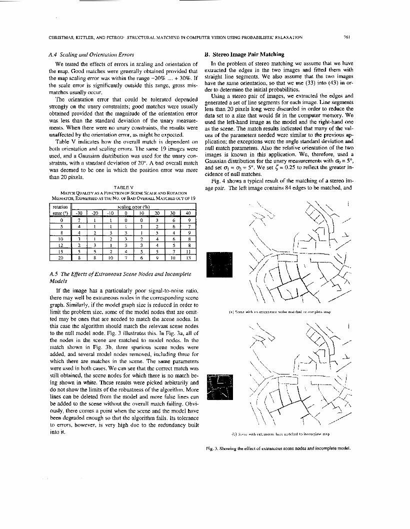
Fig. 4 shows a typical result of the matching of a stereo image pair. The left image contains 84 edges to be matched, and

I rotation (I

A.5 The Effects of Extraneous Scene Nodes and Incomplete Models

If the image has a particularly poor signal-to-noise ratio, there may well be extraneous nodes in the corresponding scene graph. Similarly, if the model graph size is reduced in order to limit the problem size, some of the model nodes that are omitted may be ones that are needed to match the scene nodes. In this case the algorithm should match the relevant scene nodes to the null model node. Fig. 3 illustrates this. In Fig. 3a, all of the nodes in the scene are matched to model nodes. In the match shown in Fig. 3b, three spurious scene nodes were added, and several model nodes removed, including three for which there are matches in the scene. The same parameters were used in both cases. We can see that the correct match was still obtained, the scene nodes for which there is no match being shown in white. These results were picked arbitrarily and do not show the limits of the robustness of the algorithm. More lines can be deleted from the model and more false lines can be added to the scene without the overall match failing. Obvi- ously, there comes a point when the scene and the model have been degraded enough so that the algorithm fails. Its tolerance to errors, however, is very high due to the redundancy built into it.

[a) Scene with no extraneous nodes matched to complete map

(b) Scrnr with extraneous lines matched to incomplete map

Fig. 3. Showing the effect of extraneous scene nodes and incomplete model.


the right 69 edges. 60 matching pairs were found, of which two are incorrect. The black lines in both images are those that remained unmatched. Otherwise corresponding edges in the two images are indicated by white lines. Also in the occasional instance where two (or more) edges of one image are mapped to the same edge of the other, one of the edges will be obscured.

Fig. 4. Matching edge segments from a stereo pair of images.

C. Algorithm Performance

We see from (45) and (44) that the computation consists of two parts: The precalculation of the compatibility coefficients and the relaxation process. Each has a complexity proportional to the square of the total possible number of matches, which we denote as n,. Thus, n, I NM, the product of the number of scene and model nodes, the equality being obtained when no matches have been pruned.

The calculation of the compatibility coefficients is thus a fixed overhead; with our algorithm it is usually the more time- consuming part of the computation, taking for example about 10 sec on a Sun Sparcstation 10 for an example that had a total of 951 possible matches. The coefficients also dominate the memory consumption, occupying n, floating-point words.

The computation for each iteration essentially requires one multiply-accumulate for each match; in the example above each iteration took about 800 msec on the same machine. Fig. 5 shows a histogram for the number of iterations required for convergence for the road-matching example, accumulated over about 3,600 experiments using different parameters and scene locations. The relaxation process for this test was stopped when for each scene node there was one match that had a probability of at least 0.9.

1x. DISCUSSION AND CONCLUSIONS

We have developed a theory of probabilistic relaxation for structural matching. By using as our starting point the Maxi- mum A Posteriori probability rule, we were able to specify completely the relaxation algorithm, including the calculation of the compatibility coefficients.

The theory rests heavily on the assumption that binary relations between primitives are adequate for the description of the whole structure and that higher order relations are superfluous. This is certainly true if the binary relations are defined in such

a way that their knowledge uniquely defines the absolute position (and thus the identity) of a primitive (object) given the absolute position of the object with respect to which the binary relations are defined. Examples of such binary relations are the relative orientation between lines, or the relative orientation, midpoint distance and size between line segments. Counter examples are relations like “object ai is on the left of object uj,” etc. If the binary relations have been chosen in the appropriate way, the number of relations needed to define the whole structure fully is given by the square of the graph size, as opposed to an exponentially growing number if higher order relations were to be involved. This considerably reduces the computational overhead.

800

600

400

200

0 5 10 15 20 25 0

Fig. 5. Histogram of the number of iterations required for convergence.

In the specific application we discussed in this paper, further redundancy would be possible if a much more reliable line map could be extracted from the image. For example, humans could match road networks by simply matching two or three roads which are at specific orientations from each other. Similarly, objects often can be recognized by recognizing a small subpart of them. In principle, this should be possible in machine vision too. However, machine vision data are too noisy and the matching process has to rely on the cooperative matching of all visible subparts. That is why, in the algorithm that we implemented, all binary relations between objects are taken into consideration. This may sound excessive; however it results in a very robust algorithm which, as shown in the previous section, can cope with very noisy data containing


many extraneous line segments as well as missing whole parts of the matched networks.

Because of the choice of unary and binary relations, our matching is invariant to translation and rotation but not to scale changes. Clearly the results are not affected if both networks are changed by the same scale factor. However, they will deteriorate drastically when scales are changed relative to each other by a factor larger than about 20%. Our work is aimed at performing inexact matching under distortions caused by noise, but not at dealing with rubber-like shape changes. This is because the constraints used are geometric rather than topological.

The computational algorithm for the matching may be paral- lelized at different levels, according to the requirements of the available hardware. Thus, for a coarse-grained parallelism we may implement the update rule for each scene node on a sepa- rate processor; alternatively on vector-processor or SIMD architectures we may treat the multiply-accumulate operation at the heart of the support function as a vector process.

ACKNOWLEDGMENTS

This work was supported by IED and Sciences and Engi- neering Research Council, project number IED-1936. The images were kindly provided by the Defense Research Agency, RSRE, U.K.

REFERENCES

D.H. Ackley, G.E. Hinton, and T.J. Sejnowski, “A learning algorithm for Boltzmann machines,” Cognitive Science, vol. 9, pp. 147-169, 1985. H.S. Baird, Model-Based Imuge Matching Using Location. MIT Press, 1985. H. Ballard and M. Brown, Computer Vision. Prentice-Hall, 1982. P.J. Besl and R.C. Jain, “Three-dimensional object recognition,” Com- puting Surveys, vol. 17, pp. 75-145, 1985. J.R. Beveridge and E.M. Riseman, “Hybrid weak-perspective and full- perspective matching,” Cunf Computer Vision and Pattern Recogni- tion, pp. 432-438, 1992. B. Bhanu, “Representation and shape matching of 3-D objects,” IEEE Trans. Pattem Analysis and Machine Intelligence, vol. 6, no. 3, pp. 340-351, 1984. B. Bhanu and O.D. Faugeras, “Shape matching of two-dimensional objects,” IEEE Trans. Pattern Analysis and Machine Intelligence,

E. Bienenstock, “Neural-like graph-matching techniques for image processing,” D.Z. Anderson, ed., Neural Infurmation Processing Sys- tems, pp, 21 1-235, Addison-Wesley, 1988. A. Blake, “The least disturbance principle and weak constraints,” Pat- tern Recognition Letters, vol. 1, pp. 393-399, 1983.

vol. 6, pp. 137-156, 1984.

- _ [lo] A. Blake and A. Zisserman, Visual Reconstruction. Cambridge, Mass.:

MIT Press, 1987. [ l 11 R.C. Bolles, “Robust feature matching through maximal cliques,” Proc.

Soc. Photo-Optical Instrument Engineers, vol. 182, pp. 140-149, Apr. 1979.

[12] K.L. Boyer and A.C. Kak, “Structural stereopsis for 3-D vision,” IEEE Trans. Pattern Analysis and Muchine Intelligence, vol. 10, pp. 144-166, 1988.

[13] T.A. Cass, “Polynomial-time object recognition in the presence of clut- ter, occlusion, and uncertainty,” Second European Cont Computer Vision, Santa Margherita Ligure, Italy, May 1992, pp. 834-842. Springer-Verlag, 1992.

[ 141 L.S. Davis, “Shape matching using relaxation techniques,” IEEE Trans. Pattern Analysis and Machine Intelligence, vol. 1, no. 1, pp. 60-72, Jan. 1979.

[I51 O.D. Faugeras and M. Berthod, “Improving consistency and reducing ambiguity in stochastic labeling: An optimization approach,” IEEE Trans. Pattern Analysis and Machine Intelligence, vol. 3, pp. 412-423, Apr. 1981.

161 O.D. Faugeras and M. Hebert, “The representation, recognition, and locating of 3-D objects,” Int’l J . Robotics Research, vol. 5 , no. 3, pp. 27-52, 1986.

171 M. Fischler and R. Elschlager, “The representation and matching of pictorial structures,” IEEE Truns. on Computers, vol. 22, pp. 67-92, 1973.

181 D. Geiger and F. Girosi, “Parallel and deterministic algorithms from MRF‘s: Surface reconstruction,” IEEE Trans. Pattern Analysis and Machine Intelligence, vol. 13, no. 5 , pp. 401-412, May 1991.

[I91 S. Geman and D. Geman, “Stochastic relaxation, Gibbs distributions, and the Bayesian restoration of images,” IEEE Trans. Pattern Analysis and Machine Intelligence, vol. 6, pp. 721-741, 1984.

[20] D.E. Gharhaman, A.K.C. Wong, and T. Au, “Graph optimal monomor- phism algorithms,” IEEE Trans. Systems, Man, and Cybernetics, vol. 10, no. 4, pp. 181-188, Apr. 1980.

[21] B. Gidas, “A renormalization group approach to image processing problems,” IEEE Trans. Pattern Analysis and Machine Intelligence, vol. 11, pp. 164-180, 1989.

[22] W.E.L. Crimson and T. Lozano-Perez, “Localizing overlapping parts by searching the interpretation tree,” IEEE Trans. Puttem Analysis and Machine Intelligence, vol. 9, pp. 469482, 1987.

[23] E.R. Hancock and J. Kittler, “Edge labeling using dictionary-based relaxation,” IEEE Trans. Pattern Analysis and Machine Intelligence, vol. 12, pp. 165-181, 1990.

[24] J.J. Hopfield, “Neurons with graded response have collective computational properties like those of two-state neurons,” Proc. National Acad- emy cf Science, USA, vol. 81, pp. 3.088-3,092. 1984.

[25] R.A. Hummel and S.W. Zucker, “On the foundations of relaxation labeling process,” IEEE Trans. Pattern Analysis and Machine Intelligence, vol. 5 , no. 3, pp. 267-286, May 1983.

[26] R.L. Kirby, “A product rule relaxation method,” CGIP, vol. 13, pp. 158-189, 1980.

[27] S. Kirkpatrick, C.D. Gellatt, and M.P. Vecchi, “Optimisation by simulated annealing,” Science, vol. 220, pp. 671480, 1983.

[28] J. Kittler and J. Foglein, “On compatibility and support functions in probabilistic relaxation,” CVGIP, vol. 34, pp. 257-267, 1986.

[29] J. Kittler and E.R. Hancock, “Combining evidence in probabilistic relaxation,” Int ’1 J. Pattern Recognition und Artificial Intelligence, vol. 3, pp. 29-51, 1989.

[30] C. Koch, J. Marroquin, and A. Yuille, “Analog ‘neuronal’ networks in early vision,” Proc. National Academy of Science, USA, vol. 83, pp. 4,2634,267, 1986.

[31] S.Z. Li, “Matching: invariant to translations, rotations and scale changes,” Pattern Recognition, vol. 25, pp. 583-594, 1992.

[32] S.Z. Li, J. Kittler, and M. Petrou, “On the automatic registration of aerial photographs and digitised maps,” Optical Engineering, vol. 32, no. 6, pp. 1,213-1,221, June 1993.

[33] S . Peleg, “A new probabilistic relaxation scheme,” IEEE Trans. Puttern Analysis und Machine Intelligence, vol. 2, pp. 362-369, 1980.

[34] M. Petrou, “Optimal convolution filters and an algorithm for the detection of wide linear features,” IEEE Proc.-I, vol. 140, no. 5 , pp. 331- 339, Oct. 1993.

[35] B. Radig, “Image sequence analysis using relational structures,” Pattem Recognition, vol. 17, pp. 161-167, 1984.

[36] A. Rosenfeld, R. Hummel, and S. Zucker, “Scene labeling by relaxation operations,” IEEE Trans. Systems, Man, and Cybemetics, vol. 6, pp. 4 2 M 3 3 , June 1976.

[37] L.G. Shapiro and R.M. Haralick, “Structural description and inexact matching,” IEEE Trans. Pattern Analysis and Machine Intelligence, vol. 3 , pp. 504-519, Sept. 1981.

[38] F. Stein and G. Medioni, “Structural indexing: Efficient 3-D object recognition,” IEEE Truns. Pattern Analysis and Machine Intelligence, vol. 14, pp. 125-145, 1992.

IEEE TRANSACTIONS ON PATTERN ANALYSIS AND MACHINE INTELLIGENCE, VOL. 17, NO. 8, AUGUST 1995

S. Ullman, “Relaxation and constraint optimization by local process,” Computer Graphics and Image Processing, vol. 10, pp. 115-195, 1979. N.M. Vaidya and K.L. Boyer, “Stereopsis and image registration from extended range features in the absence of camera pose information,” Con5 Computer Vision and Pattern Recognition, pp. 76, 82. W.M. Wells, “MAP model matching,” Con$ Computer Vision and Pattern Recognition, pp. 486-492, 1991, A. Witkin, D. Terzopoulos, and M. Kass, “Signal matching through scale space,” Int’l J . Computer Vision, vol. 1, pp. 133-144, 1987. K. Yamamoto, “A method of deriving compatibility coefficients for relaxation operators,” Computer Graphics and Image Processing, vol. 10, pp. 256-27 1, 1979. B. Yang, W.E. Snyder, and G.L. Bilbro, “Matching oversegmented 3-D images to models using association graphs,” Image und Vision Comput- ing, vol. 7, pp. 135-143, 1989. S. Zucker and J. Mohammed, “Analysis of probabilistic labeling process,” IEEE PRIP Con$, Chicago, USA, pp. 167-173, 1978.

Bill Chr stmas received his first degree in engineering science from Oxford University in 1972 He worked for many years as a research engineer for the Bntish Broadcasting Corporation in the field of telecommunications, where he developed an interest in real-time systems In 1986 he moved to BP Re- search International. There he initially worked on hardware aspects of large-scale parallel-processing computer architectures and subsequently developed real-time image processing and machine vision applications While at BP he received an MSc degree in signal processing and machine intelligence

from the University of Surrey Since 1992 he has been a research fellow with the Vision, Speech, and Signal Processing group at the University of Surrey, where he has been studying for a PhD on the use of probabilistic methods for geometric feature matching.

Josef Kittler obtained his BA in electrical engineering in 1971, his PhD in pattern recognition in 1974, and his ScD in 1992, all from the University of Cambridge. He has been a research assistant in the engineering department of Cambridge University (1972-1975); SERC research fellow, University of Southampton, Department of Electronics (1975- 1977); Royal Society European research fellow, Ecole Nationale Superieure de Telecommunications, Paris (1977-1978); IBM research fellow, Balliol College, Oxford (1 978-1980); principal research associate, SERC Rutherford Appleton Laboratory

(1980-1984); and principal scientific officer, SERC Rutherford Appleton Laboratory (1985). He also worked as the SERC coordinator for pattern analysis (1982) and was Rutherford research fellow in Oxford University, Department of Engineering Science (1985). He joined the Department of Electrical Engineering of Surrey University in 1986 as a reader in information technology and became professor of machine intelligence in 1991. He is head of the Vision, Speech, and Signal Analysis group at the Department.

He has worked on various theoretical aspects of pattern recognition and on many applications including system identification, automatic inspection, ECG diagnosis, remote sensing, robotics, speech recognition, character recognition, and line-drawing processing. His current research interests include pattern recognition, image processing, and computer vision.

Dr. Kittler has coauthored a book entitled Pattern Recognition: A Statisti- cal Approach published by Prentice-Hall. He is a member of the Committee of the British Machine Vision Association and Society for Pattern Recogni- tion and a representative of the British Machine Vision Association and Society for Pattern Recognition for the International Association for Pattern Recognition. Finally, he is a member of the editorial boards of IEEE Trans- actions on Puttern Analysis und Machine Intelligence, Pattern Recognition Journal, Image and Vision Computering, Pattern Recognition Letters, and Pattern Recognition and A rtijicial Intelligence.

Maria Petrou received her BSc in physics from the University of Thessaloniki, Greece, in 1975 and her PhD in astronomy from the University of Cam- bridge, U.K., in 1981. She has been working on computer vision since 1986 and has published more than 50 papers, half of them in refereed journals, on remote sensing, low-level vision, feature extraction, texture analysis, Markov random fields, probabilistic relaxation, industrial inspection, etc. She is a senior lecturer at the Department of Electronic and Electrical Engineering of Surrey University, a mem-

ber of the British Machine Vision Association, the Society of Optical Engi- neering, and the IEEE.

Dr. Petrou is on the refereeing panel of many international journals, has served on the program committee of several international conferences, is associate editor of IEEE Transactions on Imuge Processing, and is editor of the newsletter of the International Associution of Pattern Recognition.

structural matching in computer vision using … kittler, and petrou: structural matching in...

Documents