1*NOAA/NMFS/NEFSC, Woods Hole, MA 02543

cProfessional and Technical Services, Inc., Norfolk VA, 23502

1

Structure and transport of alongshelf currents across the southern flank ofGeorges Bank during late summer, 1982

RONALD J. SCHLITZ*1, JAMES P. MANNING* and KESTON W. SMITHc

Abstract--An array including seven moorings was in place between 10 August and 25 September,

1982 on southern Georges Bank. This was the second setting in cooperation with the Warm-Core

Rings Experiment (WCRII). Ten of the records from the Vector Averaging Current Meters

(VACMs) were complete. Short-term drifters with window-shade drogues at 10 m were launched

and recovered seaward of the shelfbreak (200 m) to document flow of shelf water across

bathymetry. Winds were available for this period from NOAA buoy 44003 at the southwestern

corner of Georges Bank near the array. The major structure in the subtidal flow is an alongshelf

maximum toward the west (mean speed ~ 27 cms -1 with bursts often > 30 cms -1) at the shelfbreak

front (~ 100 m); the shelfbreak jet. The first two modes in empirical orthogonal analysis of the

cross-bank structure contain 82% of the variance. Mode 1 is associated with the large-scale

alongshelf current and is partially correlated with local winds. Mode 2, generally not correlated

with wind, may be generated by features initiated by the Gulf Stream. The current record at the

northern periphery of the warm eddy or remnant of a warm-core ring has a mean velocity of 5 cms -1

toward the east for the period, opposite the general circulation over the shelf. Elsewhere the

circulation over the shelf seemed minimally affected even with the proximity of the offshore

feature.

A mean estimate for volume transport of shelf water during the period is 0.83 ± 0.2 sv with

2

periods of greater than 1 sv related to NE winds leading by six hours. While a bias is possible due

to undersampling of the velocity field, this mean value and variability during late summer are

higher than previously reported estimates for transport of shelf water. This is primarily due to the

additional contribution of the shelfbreak jet near the 100 m isobath. Confidence limits for the

transport were calculated by two independent methods, geometric weighting and block estimation

by universal kriging.

Keywords: Wind-driven currents; Volume transport; Current meter data; Hydrography; Georges Bank;

Southern flank

INTRODUCTION AND MOTIVATION FOR EXPERIMENT

One source of mortality for planktonic species is removal from a favorable habitat (e.g., Iles and

Sinclair, 1982). Among the hypothesized physical mechanisms for dislocation of pelagic organisms

from Georges Bank are alongshore transport into the Middle Atlantic Bight and entrainment of shelf

water by Gulf Stream warm-core rings, i.e., advection of shelf water beyond the normal position of the

shelf/slope front and subsequent loss from the coastal ocean. The organism associated with the

entrained shelf water would eventually be within a hostile environment for survival. The overall

importance of this loss on subsequent recruitment of year-classes of fish has been discussed often,

always including caveats. For example Cohen et al. (1986) attempt to partition various physical effects

on recruitment of haddock for Georges Bank. They conclude that different advective processes,

including entrainment by warm-core rings, could dominate at different times. Their analysis was

complicated because a strong storm with high winds occurred concurrently with the passage of a

warm-core ring. Direct measurements showing the intensity and frequency of entrainment and

distribution of shelf larvae beyond the shelf break south of Georges Bank were not available to help

3

their interpretation. On the other hand, flow along the isobaths from Georges Bank to the Middle

Atlantic Bight results in an unequivocal loss for populations of zooplankton on the southern flank. This

is a continuous mechanism operating throughout the year on plankton within the water column. Mean

speeds along isobaths of 10-20 cms-1 would remove plankton from the southern flank in approximately

a week unless counteracted by biological processes. The balance between these various mechanisms

affecting mortality of zooplankton and ichthyoplankton remains an open question.

Georges Bank is a broad, shallow section of continental shelf that separates the deeper Gulf of

Maine from the main body of the Atlantic Ocean. While the mean circulation is generally clockwise

around the bank continuing into the Middle Atlantic Bight, some turning into Great South Channel is

shown during the stratified season (Manning and Beardsley, 1996). Butman and Beardsley (1987)

present a seasonal cycle for circulation around Georges Bank, peaking in late summer. However,

Limeburner and Beardsley (1996) could not confirm the seasonal cycle in circulation from a series of

drifters with drogues at 5 m and 50 m. Also, no drogue at the 50 m level recirculated around Georges

Bank. Significant fluctuations at higher frequencies occur due to tides, time-varying winds, and

variations in density structure. Changes in the position of both the tidally mixed front (in the stratified

season) and the shelf/slope front along the southern flank result in deviations from the classical gyre-like

flow. These may provide the primary mechanism for seasonal and interannual differences in the

retention and loss of ichthyoplankton and their prey.

The details of frontal dynamics as summarized by Flagg (1987) include several processes.

These include a seasonal migration of the front bankward from winter through the summer, the

presence of the cold band in the deep water just shoreward of the shelf/slope front in spring and

4

summer, the potential effects of warm-core rings throughout the year, and other small scale processes

such as calving, the detachment of parcels of shelf water into slope water (Garvine et al., 1988).

However, on the southern flank, few reported experiments of long duration have sufficient spatial

resolution to determine the structure of the alongshelf currents or to calculate volume transports.

Nearby, toward the west, Beardsley et al. (1985) report on an array of current meters south of

Nantucket for 13 months. Also Manning and Beardsley (1996) discuss a synthesis of many individual

settings of current meters across Great South Channel and the southern flank of Georges Bank.

A series of cruises was completed by NMFS in coordination with the Warm-Core Ring project

sponsored by NSF. During one cruise (June 1982), a Multiple Opening Closing Net Environmental

Sensing System (MOCNESS) with an opening of one square meter sampled plankton at stations on the

continental shelf and within entrained shelf water associated with ring 82-B. These stations were in the

Middle Atlantic Bight off the Delmarva Peninsula. LeBlanc (1986) reports that 12 species of larval fish

were identified within entrained shelf water seaward of the 200 m isobath. For example, the mean

standard lengths for P. Triacanthus (butterfish) of 4.3 mm and M. bilinearis (silver hake) of 4.9 mm are

sizes associated with recently hatched larvae (unfortunately comparative samples from the other cruises

in the series were lost). Schlitz (1999) concludes from examining the temperature-salinity properties of

ring-entrained water that the predominant source is along the outer continental shelf seaward of the cold

band (Houghton et al., 1982), but at times includes a contribution from the seaward side of the cold

band.

Besides the shipboard physical and biological sampling completed during the Warm-Core Ring

project, two moored arrays were set along and across the shelf break to examine the interaction

5

between rings and shelf water. The first of these arrays (WCRI) was in place between 15 April and 1

July 1982 south of New England. Ramp (1989) reports on current variability in relation to the

radiation of barotropic topographic waves from ring 82-B. He also concludes from temperature

measurements that two months are needed to restore the shelf/slope front to a "normal" position after

passage of a warm-core ring. Ramp (1986) proposes two mechanisms that could trigger entrainment

of shelf water; horizontal shear instability along the front formed between the ring water and shelf water

and wakes resulting from Rossby waves.

The second array (WCRII) sampled currents and temperature along the southern side of

Georges Bank between 10 August and 25 September, 1982. The placement of WCRII was

determined after sea-surface temperatures derived from AVHRR data indicated that a warm-core ring

was present in the area. Subsequently, AVHRR images showed that the feature was more likely a

complicated structure on the northern periphery of the meandering Gulf Stream rather than an isolated

ring. The feature interacted continuously with the main Gulf Stream located toward the south during

deployment (Figure 1). Detailed interpretation of a time series of AVHRR data was hampered by

clouds.

This report emphasizes the structure of alongshelf flow, effects of wind on the circulation, and

estimates of variations in transport during WCRII. The interval of time covered by this moored array,

although short, is important since maximum stratification generally occurs during late summer and the

total alongshelf flow should also reach a maximum (Butman and Beardsley, 1987).

DATA

WCRII was deployed on the southern flank of Georges Bank between 10 August and 25

6

September, 1982. The array had both alongbank and crossbank components (Figure 2). Basic

information for each instrument and corresponding statistics are presented in Table 1a. All moorings

were recovered but the current meter at site 4 lost when wire rope parted during retrieval of the

instrument. All other sites returned records from the instrument near the surface (10 m) except site 3 in

which the tape failed to advance. In addition subsurface instruments were at site 3 (40 m, 100 m, and

305 m) and site 6 (35 m and 85 m). Vector-averaging current meters (VACMs) were used at each

location to record a vector-averaged velocity and instantaneous temperature every 15 minutes. All

data were processed by the Woods Hole Oceanographic Institution using the standard data analysis

system for oceanographic time series. The 15-minute samples were checked for gaps and bad points

and hourly time series were generated.

An additional check was made on these data for known tides. The most energetic currents on

Georges Bank occur at the semi-diurnal period (M2), increasing in amplitude from the southern flank to

the northern edge (e.g., Manning and Beardsley, 1996; Moody et al., 1984). The amplitudes, semi-

major and semi-minor axes, and phases of currents at the M2, O1, K1, N2, and S2 periods were

determined for each instrument in the array. M2 values are consistent with previous results ranging

from 8 cms-1 at the edge of the continental shelf to 53 cms-1 at the northern end of the array near the

tidally mixed front. For example, site 5 nearly corresponds to site K in Moody et al. (1984). The

semi-major axes of the tidal ellipses from these sites agree to within 1%, and the semi-minor axes to

within 10%. The orientations of the tidal ellipses differ by 1.1E T. Although the results are expected, it

gives additional confirmation of the quality and consistency of these data.

Low-passed time series were then calculated using a digital filter with a half-point at 33 hours,

7

PL33 (Flagg et al., 1976), which removes tides (Table 1b). The east and north components of velocity

were rotated onto principal axes to determine the direction of low-frequency variability (Table 2a).

Also axes relative to the local overall mean alongshore current at each instrument were determined for

further analyses (Table 2b).

Winds for the region were taken from NOAA Buoy 44003, at 40E48' N , 68E30' W (Figure

2). Anemometers were situated at 5 m above the surface as part of the standard General Service Buoy

Payload (GSBP). On this system both wind speed and direction were sampled at 1 Hz and averaged

every 8.5 minutes. These data were then averaged to hourly time series. Also, peak hourly gusts were

recorded. Wind stress was calculated from the hourly time series (see Manning and Strout, this issue,

for a summary of methods).

Temperature and salinity profiles were collected using a continuously recording

Conductivity/Temperature/Pressure (CTD) instrument during cruises that set and recovered the

moorings. Water samples were collected at selected depths during casts. Salinities, which were

determined by a precision conductive salinometer, were then used to check the calibration of

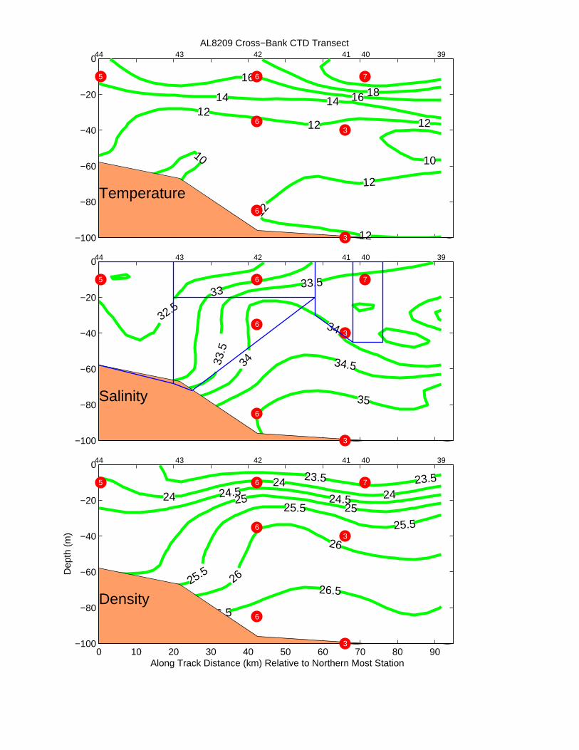
conductivity data. Temperature, salinity, and density sections along the mooring line are shown in Figure

3. Shelf water is defined by salinities < 34; based on the range of salinities generally found on Georges

Bank inside the shelfbreak front (Schlitz, 1999).

During the cruise of R/V Albatross IV to set the moored array, five surface buoys drogued at

10 m were launched and tracked for short periods. Each consisted of a window-shade approximately

220 ft2 (21 m2) in area, attached by thin line to a high-flyer at the surface, approximately 1 ft2 (0.09 m2)

in cross-sectional area. The purpose was to follow the offshelf movement in an entrainment associated

8

with a warm-core ring. The resulting data are summarized in Table 3. Four of the five drogues (D1,

D3, D4, D5) were launched in a surface layer of shelf water at oceanic depths greater than 200 m. The

fifth, the easternmost (D2), was always in water with salinity > 34 near the boundary between shelf

water and slope water. Temperature and salinity characteristics at the drogues were determined

through a series of additional CTD casts.

A T-S diagram for all stations in the region is presented in Figure 4. The demarcation between

shelf water and slope water occurs at a maximum temperature of about 21.7EC for these data.

RESULTS

Subtidal temperature and currents

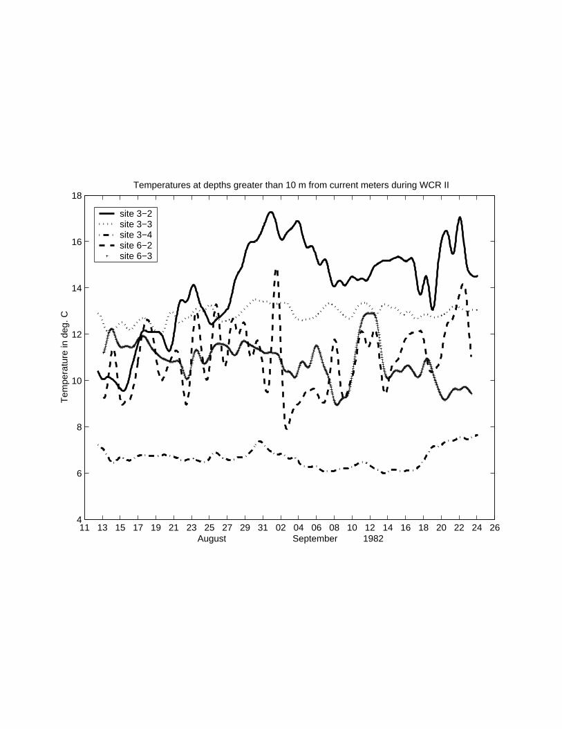
The low-passed temperatures from thermisters on each current meter are shown for the

duration of the moored array (Figure 5). Some noteworthy features are within the time series.

Temperatures at 10 m’s from sites one and two, located along the ~ 325 m isobath, decrease markedly

early in the record. Maximum temperatures for both, 24.7EC at site 1 and 25.2EC at site 2, occur at

the beginning of the record. These temperatures can be associated with water from the warm feature of

the Gulf Stream (Figure 4). One CTD station taken within this feature produces a limb on the T-S

diagram with temperatures > 25E C. Temperatures then decrease to minimums of 15.6EC at site 1

and 16.8EC at site 2. These temperature changes result from inflow of cooler shelf water coincident

with southward recession of the feature. The inverse trend happens at site 3 (record at 40 m), warming

from 8.5EC to 17.2EC as the cooler shelf water from an earlier entrainment of shelf water is displaced.

The near-surface record at site 6 has variability typical of measurements near the shelfbreak front (e.g.,

9

Flagg, 1987). Also a characteristic signature of the cold band, temperatures around 10EC, is seen at a

depth of 35 m on site 6. Although site 7 was positioned to sample changes in the slope water regime

associated with variability in loss of shelf water by entrainment, only shelf water persisted until the end

of the record. Resolution of spatial variability at a short scale above the thermocline between sites 3

and 7 was not possible with the loss of the record at 10 m on mooring 3.

The overall means of low-passed currents during the WCRII array are shown in Figure 2 and

Table 2. Currents at sites 5 and 6 on the shelf follow the general trend of the local mean topography.

Largest velocities, 27 cms-1 toward 250E T and 19 cms-1 toward 255E T, were found on mooring 6 at

depths of 10 m (6-1) and 35 m (6-2) respectively. The means at sites 1 and 2, both near the 325 m

isobath, suggest convergence between the moorings during two months. Site 1 is opposite the overall

shelfwide flow toward the southwest resulting from the influence of the circulation associated with the

Gulf Stream interaction. The velocities at site 3 show considerable variation with depth. Influence of

the local topography is possible since the mooring is located on the continental slope between Powell

and Lydonia Canyons (Figure 2). The mean at site 7 is small and toward the north.

Individual currents at each instrument in the array can be seen from the progressive vectors

(Figure 6). Flow is generally parallel to the bathymetry toward the southwest at all locations except site

7 in 895 m of water where net movement was small, and site1 described above. Intensification of flow

in deeper water over the southern flank is clearly portrayed. The largest movements toward the

southwest are at 10 m and 35 m depths for site 6 at 100 m on the southern flank. These are the only

locations where low-passed currents exceeded 30 cms-1 during periods of low wind. This structure

has only recently (Linder and Gawarkiewicz, 1998, Pickart et al., 1998, Manning et al., 1999) been

10

called the shelfbreak jet though clearly it is a permanent part of the alongshelf circulation (e.g., Flagg,

1977). The core of the current is generally centered between 100 m and 120 m in the Middle Atlantic

Bight (Linder and Gawarkiewicz, 1998), shallower than the large increase in bottom-slope at

approximately the 200 m isobath, defined as the shelfbreak for this region.

Specific drogues were followed between 15 hours and 70 hours (Table 3). D2 was recovered

after a series of four CTD stations taken at the position of the drogue showed only slope water

(surface salinity of 34.76 and temperature of 22.31EC at the final station). D1 was also recovered after

leaving shelf water. D3 - D5 were recovered earlier than planned due to unanticipated needs of

another project. Except for a single station alongside D5 with a salinity at the surface of 32.95,

increasing to 33 at 5 m, all salinities for shelf water were greater than 33 at the drogues indicating a

source near the shelfbreak front. In addition, the near-surface temperatures associated with these

salinities were everywhere greater than 19.5EC and predominately greater than 20EC (Figure 4).

These T-S values are found near the surface above the 100 m isobath as shown in Figure 3.

Mean velocities over the duration of each drogue are shown in Figure 7, superimposed on the

surface temperature field from an AVHRR image during the period. Low-passed velocities at 10 m

from each current meter for the hour closest to the AVHRR transit are also included. The overall drift

determined from the drogues appears decoupled from the currents over the southern flank of Georges

Bank during this time. Excepting D5, which is close to the 34 isohaline at a western boundary of

entrained shelf water, there is no cross-isobath flow of shelf water potentially associated with the

nearby circulation of water originating from the Gulf Stream. The mean direction of D3 is consistent

with the northern edge of a cyclonic ringlet described by Kennelly et al. (1985), albeit at a lower speed.

11

There is no further information in the currents to confirm this. D1, D2, and D4 moved opposite the

mean regional circulation.

Wind-driven response

Wind-driven response of currents on the southern side of Georges Bank shows significant

variability during the summer. This association can be seen through examples. On 25-26 August 1982

“strong” SW-W winds ( hourly averages >15 kt (7.7 ms-1, 0.1 Pa) for 14 hours including three hours

with $20 kt (10.3 ms-1, 0.18 Pa)) caused a response above the thermocline along the southern flank

consistent with Ekman forcing (Figure 8). Surface currents rotated toward the south at each location,

first at site 7 where the mean current was low. During this period, maximum currents at sites 5, 6, and

7 exceeded 30 cms-1 in the upper layer, suggesting significant southward excursions (>26 kmd-1) for

water on the southern flank of Georges Bank. Spin-up time coincides reasonably with the initiation of

Ekman velocity at the surface, 7-8 hours for this latitude. Although speeds for wind at 7.7 - 10.3 ms-1

may not seem high in the yearly cycle for Georges Bank, the NOAA National Data Buoy Center

(NDBC) (unpublished data) calculates an average wind speed of 3.8 ms-1 during August at buoy

44003 for data collected between 1977 and 1983. Also, the average of hourly peak gusts for August

was 4.1 ms-1 for data collected between 1981 and 1983. So this burst of southwesterly winds was at

least double the mean condition from the time series at 44003.

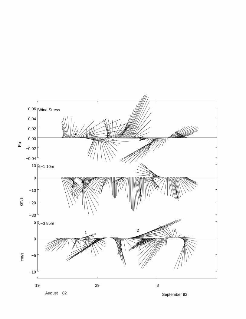
On this and two other occasions these wind-driven offshore flows in the upper layer coincided

with return flow at depth below the shelfbreak front. These three events are labeled in the bottom panel

of Figure 9a where periods of northeastward wind stress forced southward flow at instrument 6-1 with

northward flow at 6-3. Details are shown in Figure 9 b-d. At the beginning of each episode the total

12

low-passed current at 6-1 begins to rotate cyclonically from the mean southwesterly direction. This

rotation is understood as the vector summation of the general alongshelf current and adjustment of the

current vector near the sea surface following an Ekman response to the onset of wind. As the event

progressed and the wind continued rotating toward the east, flow with an onshelf component developed

at 6-3 when the wind stress was between 070E T and 105ET. Each instance was accompanied by a

rise in temperature consistent with warmer slope water offshelf at this depth (Figure 5).

This reversal of flow at depth was persistent enough to be captured in the spectral statistics.

The coherence calculations between the north component of velocity at 6-1 and 6-3 showed a phase

difference of approximately 180E, using overlapping segments of 10 days and averaging over four

frequency bands. Also, the statistical relationship between eastward wind and the northward current at

6-3 was in phase with a transfer function of 84 ± 42 cms-1Pa-1, following Bendat and Piersol (1986) for

confidence intervals. Although this presumed upwelling does not happen continuously, the transfer

function is only one third that near the surface (259 ± 70 cms-1Pa-1), and the statistics are not strongly

significant due to limited degrees of freedom (10), the process represents an additional subtle

intermittent flow across isobaths.

Wind stress was calculated for 15E T intervals in direction, and spectral quantities between

wind and currents at mooring 6 estimated to determine the component of the wind most effective in

driving the near-surface currents over the southern flank. Significant values resulted for certain

rotations, again noting the limitation in the number of degrees of freedom. The north/south variability

recorded at 6-1 was best correlated with no rotation of the east/west wind (Figure 10a) in the 1-2 day

band. The phase of approximately 180 ± 25E T at the 95% confidence level indicates a southward

13

flow responded to a west wind (eastward stress). East/west variability recorded at 6-1 was most

coherent with the northeast/southwest component of the wind (Figure 10b). In this instance the phases

are insignificantly different from zero showing northeastward wind stress driving eastward flow and

southwestward wind stress driving westward flow. These results are consistent with Noble et al.

(1985) for data collected across four years on the southern flank of Georges Bank. The period of this

east/west process was longer (3-5 days vs. 1-2 days) but not as effective with transfer functions of

136 ± 55 cms-1Pa-1 versus 259 ± 70 cms-1Pa-1.

Estimates of residual velocities from the tracks of drogues required removal of slippage (Geyer,

1989; Allen, 1995) and the large wind-driven component seen in the currents at 10 m from the mooring

sites. First, the transfer functions between current and wind at 7-1, -177 ± 64 cms-1Pa-1 and 355 ±

129 cms-1Pa-1, were applied to the eastward and northward wind stress, respectively, to estimate the

southward and eastward components of wind-driven flow. The slippage between the window-shade

and flow was then needed.

Previous estimates of slippage for drifters (Geyer, 1989; Allen, 1995) are between 0-6 cms-1

depending on both configuration of the drifter and the wind/wave conditions. Since slippage for a

window-shade drifter with a high-flyer has apparently never been measured, a middle value of 3 cms-1

in the downwind direction was chosen for the correction. Because the wind was oriented in the

alongshelf direction during the drifter deployment, uncertainty in the magnitude of slippage should only

minimally affect any estimate of crossbank residual velocity.

The resulting residuals (total velocity - wind-driven component - slippage) show a mean flow

toward the southern flank of Georges Bank at about 5 cms-1 (Figure 11) for the drifters set near the

14

200 m isobath. The direction for D3 remains compatible with a location at the northern side of a small

cyclone in the entrained shelf water. Consistency in the directions of the three drogues (D1, D2, D4)

and the residual current for site 7 at 10 m for the same period is surprising, particularly with the warm

anticyclonic feature in close proximity. Note in particular that the direction for D5 reverses substantially

once the wind-driven component was removed.

EOF analysis

Empirical orthogonal functions showing the variance in a group of time series were determined

for the portion of the array across the shelf (sites 5, 6, 3, and 7). The first two modes for structure of

the alongshelf component of low-passed currents, illustrated in Figure 12, account for 82% of the total

variance, 63% in mode 1 and 19% in mode 2. Mode 1 represents the large scale alongshelf flow,

peaking for the record at 10 m in the shelfbreak jet, site 6-1. Mode 2 is governed by the records at

depths greater than 10 m found off the shelf and represents a response to features induced by the Gulf

Stream. Highest amplitudes are found at site 3 for the depths of 100 m and 305 m. Figure 13a visually

shows correlation between the mode 1 and the alongshore winds. Coherence calculations are

significant in a band from 1.3 to 3.6 days for mode 1 but suffer from low degrees of freedom. The

significant correlation between alongshore winds and mode 1 is expected since mode 1 is comprised

mainly of shallower time series over the shelf.

Two events dominate the series in Figure 13; the northeastward stress between 25-26 August

1982 that affected both modes and the southwestward stress between 6-8 September 1982 for mode

1. These results generally agree with the interpretation of the data from NSFE79 (Beardsley et al.,

1985) which separates flow over the continental shelf, partially driven by the wind, from that at the edge

15

of the shelf. The current record at 10 m for the seaward mooring of Beardsley et al. (1985) located in

810 m of water contributes to mode 2 associated with passage of warm-core rings. The current at site

7 of the present study in 895 m of water was part of flow over the shelf, mode 1.

Transport variability

Transport of water along the continental shelf can be estimated for the duration of the array.

To place confidence limits on volume transport, two independent methods for calculations were

developed and are presented in Appendix 1. The first is based on assigning areas to each velocity

record, a traditional method for estimating volume transport. Confidence limits for the traditional

estimates are produced under the assumption that the spatial distribution of velocity is locally Gaussian

with a constant variance and a mean which changes in time. The variance of the velocity distribution in

each area is estimated from the time-averaged variance of the instruments about the area. A local mean

of velocity is estimated from the record of an instrument found within the area. The neighborhood

scheme was defined by taking the closest adjacent instruments to the instrument used for the estimate of

mean, both horizontally and vertically if other instruments were present. Instrument 6-2 was added to

the neighborhood of instrument 5-1 and instruments 3-3 and 3-4 were added to the neighborhood of

instrument 7-1 to factor in the variance in current due to depth at those sites. The second estimation is

by block universal kriging. For the kriging estimates it is assumed that the velocity structure at each

time step is the sum of a linear function and an unknown spatially-correlated noise term. The transport

estimator for each time is restricted to be a constant linear combination of data from that time, with

coefficients of the linear combination from that period chosen to minimize the prediction error.

Confidence intervals for the transport are derived from the additional assumption that the prediction

16

error of the linear predictor has a Gaussian distribution.

Figure 3 shows the areas associated with the first method superimposed on the two CTD

sections. The calculations were limited to a region approximating shelf water, salinities < 34. Likewise

kriging was limited to shelf water through pseudo-topography that treats the 34 isohaline as a solid

boundary. Extension of the area for mooring 5 into shallower water was based on drifter tracks

(Limeburner and Beardsley, 1996) showing that mean flow toward the southwest is found at depths

shallower than the 50 m isobath. The outer boundary is more problematic for the first CTD section

since shelf water extends beyond mooring 7. However the speeds are generally low as seen in the

drogue tracks, so minor underestimates for shelf water were possible. Although the east and north

components of velocity were reasonable approximations to the alongbank and crossbank directions,

transports were also calculated based on the direction of the mean alongbank current for each location.

Sensitivity of the estimates to local topography could be bounded in this way.

The estimated transports of shelf water shown in Figures 14 and 15 are based on the

distributions of salinity at the beginning and end of the time series (Case 1 and Case 2). Corresponding

weights and confidence limits computed for the geometric and kriging methods are in Table 4. Kriging

is considered less subjective since weights are not determined by positions of instruments alone and

account for the covariance structure of the currents. The mean estimated transport August-September,

1982 based on all estimates is 0.83 ± 0.2 sv. This value is generally higher than transports reported

earlier (Manning and Beardsley, 1996; Beardsley et al., 1985) for the area.

The time series of alongbank transport shows four periods (Figure 16) when all estimates were

greater than 1 sv. These were on 22 August, 29 August, 9 September, and 18-19 September.

17

Visually, all were associated with moderate NE winds blowing < 12 hours earlier at speeds between

7.2 ms-1 and 8.2 ms-1 (14 -16 kt), indicating rapid alongshelf response of transport to southwesterly

wind stress over the southern flank of Georges Bank. The representativeness of these observations

within the time series was investigated by determining the maximum correlation between the alongshelf

transport of shelf water and the vector of wind stress. The result was a correlation of 0.66 between

volume transport and wind stress toward 211E T leading by 6 hours. This correlation is well above the

value for significance at the 95% confidence level, 0.37, suggesting a primary role for wind in forcing

variability of transport along the southern flank of Georges Bank during summer. The total gain for

these conditions is 4.89 ± 1.28 svPa-1, calculated as covariance between wind stress and transport

divided by the variance of wind stress.

DISCUSSION

Vertical structure of wind-driven response

The WCRII array demonstrates that low-frequency episodes of alongshelf wind stress toward

the northeast are effective in driving the current field off the southern flank of Georges Bank. Although

contemporaneous and correlated, the vertical response at 6-3 cannot be directly forced by wind

through an Ekman layer. Under homogeneous conditions, a maximum calculated Ekman depth for the

three events is 55m well above the depth of 6-3, 85 m. Also, Werner (1999) concludes that the

Ekman response is mainly trapped above thermocline on the southern side of Georges Bank. One

explanation for the vertical structure comes from recent modeling. Greenberg et al. (1997) formulated

a three-dimensional, harmonic, finite-element model forced at low frequency by wind peaking at 0.1

18

Pa. Results show that a combination of direct Ekman forcing and pressure-gradient response results in

a significant divergence in the surface currents near the 60 m isobath on the southern side of Georges

Bank. They also note upwelling (i.e., return flow at depth to surface flow off the shelf) is particularly

strong for the southern side of Georges Bank. In addition, the modeled field of deep velocity near site 6

has a component across the bathymetry into shallower water. A region of convergence in flow near the

bottom occurs at oceanic depths of about 60 m on the southern flank. Therefore, continuity is

maintained by vertical motion in this area.

This flow across isobaths in response to winds from the southwest gives an intermittent process

that adds nutrients to the shelf from locations at the base of the shelfbreak front. Results from many

studies (e.g., Schlitz and Cohen, 1984) show that mean nitrogen content below 75 m on the southern

side is higher than levels on Georges Bank, particularly in summer. However, any quantitative estimate

of the potential flux from this process is beyond the present scope.

Residual velocity of drogues

An AVHRR image for 16 August was contoured to emphasize frontal features (Figure 11).

Residual flow for drogues D1, D2, and D4 toward the shelfbreak front at ~ 5 cms-1 is clearly shown.

These and the concurrent residual at site 7 suggest that convergence at the shelfbreak front leads to

flow toward the shelf in the surface layer at that time. The 20EC isotherm at the surface is within the

gradient associated with the shelfbreak front and crosses site 6 indicating that the shelfbreak jet was

near the 100 m isobath there. The speed of ~ 5 cms-1 is higher than the findings of Churchill and

Manning (1997). They report a convergence of 2 cms-1 onto the shelfbreak front in the same area

using sets of clustered drifters. The 21EC isotherm nearly enclosed cooler water off the shelf at D3

19

consistent with a cyclonic ringlet (Kennelly et al., 1985). Demarcation between flow affected by warm

circulation appears to coincide with the 23EC isotherm and salinities >34.6 (Figure 4). The residual

motion of D5 is not easily explained from available data.

Transport variability

The mean transport of shelf water (salinity < 34 ) calculated here, 0.83 ± 0.2 sv, is higher than

transports reported earlier for the area. This may be expected since the moorings were in place during

the time of maximum stratification on Georges Bank. Butman et al. (1987) discuss the seasonal cycle

of currents on Georges Bank, primarily seen as baroclinic adjustment to the density changes during the

stratified season, although Limeburner and Beardsley (1996) could not confirm the cycle. The only

other reported estimate of directly measured transport along the southern flank of Georges Bank is by

Manning and Beardsley (1996) for the period 27 July - 18 November, 1985. A mean value of 0.421

sv inside the 100 m isobath results from multiplying the low-passed velocity by the cross section over

which the velocity acts. The same calculation for a subset of these data, 1 September - 31 October,

produces 0.428 sv. Information is not available about the water types carried along the southern flank

within the flow. Farther to the west, Flagg (1977) estimates a transport of 0.4 sv based on three

hydrographic sections adjusted with interpolated currents at 30 m from current meters. The raw mean

estimates of 0.401 sv, inside the 100 m isobath, and 0.218 sv, outside the 100 m isobath, were

adjusted based on potential sources of error. These data were collected during the New England Shelf

Dynamics Experiment, 27 February - 3 April, 1974. A different analysis by Beardsley et al. (1976),

using the same measurements of currents and adding one additional record from the preceding year

gives 0.168 sv inside the 100 m isobath. The reasons for the difference are not clear. Finally the

20

Nantucket Shoals Flux Experiment (NSFE79) gives 0.383 ± 0.069 sv at depths between 40 m and

120 m over the 13 month time series without any detectable seasonal variations.

Here the four separate estimates for transport, based on two salinity sections and two

independent statistical models, are consistent. Questions remain about potential bias in the estimates

due to undersampling of the velocity field. For example the currents for one depth at 5-1 are used to

represent a substantial weight in the box method. There are no contemporaneous data with which to

consider potential bias. Speculation about the magnitude of an error in transport can be conducted in

the following way. Under the assumption that the basic physical processes remain within narrow

bounds for summer seasons and alongshelf scales are long on Georges Bank, vertical shear collected

nearby at the same isobath during an equivalent time for a different year can be used as a surrogate.

Such data were collected during the GLOBEC II experiment in 1997. An Acoustic Doppler Current

Profiler (ADCP) mounted on a tripod was located in 61m of water on the southern flank of Georges

Bank between 16 January and 20 August 1997. The location (40E 42.9NN, 68E 24.4NW) was about

64 km toward the west-southwest of site 5. A mean vertical distribution of alongshelf currents was

determined for the first 20 days of August, based on a vertical resolution of 1 m for the currents from

the ADCP. This mean profile was adjusted to match the time series of velocity in the direction of the

mean current at 5-1. Then estimates of transport were calculated by the geometric method. The

resulting transports are 0.63 ± 0.13 sv for Case 1 and 0.74 ± 0.15 sv for Case 2. The decreases in the

estimates of transport are 0.1 sv for Case 1 and 0.1 sv for Case 2. Similar calculations are not well

suited to universal block kriging. Under the geometric method shear correction can be interpreted

21

statistically as an adjustment for a known bias in the velocity measurement. Due to spatial

interdependence of the weighting scheme in the kriging calculation, it is not clear how to interpret the

results of an adjustment to the kriging estimates for such a bias. Notwithstanding a limitation to only the

geometric method for the calculation, the 12% - 15% reduction in transport estimates for Cases 1 and

2 are within the confidence intervals.

SUMMARY

The WCRII array on the southern flank of Georges Bank was designed to investigate

interaction of shelf waters with warm-core rings originating from the Gulf Stream. Due to the complex

structure of a meander and eddy-like feature of the Gulf Stream instead of a detached ring (Figure 1),

understanding of the intricacy of interactions was not possible through these data. However, influence

of these features originating from the Gulf Stream was shown directly in two ways. The mean current at

site 1 was toward 089E T at 5 cms-1 from 10 August through 25 September, 1982, opposing the

general circulation over the continental shelf. Concurrently temperatures at sites 1 and 2 steadily

decreased from a maximum of 24.7EC at the beginning of the record to 15.6EC on 7 September while

a meander of the Gulf Stream moved southeast away from the shelf, as interpreted from available

AVHRR images. Also a mean one-dimensional convergence was indicated along the 325 m isobath

between sites 1 and 2, inferring undefined cross-isobath flow, possibly due to meandering of the

shelfbreak front in response to anticyclonic circulation off the shelf (Figure 11). In addition shelf water,

previously entrained, was present well seaward of the normal position for the shelfbreak front.

The major feature in the circulation pattern over the southern flank of Georges Bank for this

period was the shelfbreak jet, captured in the current records at site 6 in 100 m of water. The mean

22

speeds at 6-1 (10 m) and 6-2 (35 m) were 27 cms-1 and 19 cms-1 toward the WSW respectively. The

velocities of Beardsley et al. (1985) for the shelf south of Nantucket, Manning and Beardsley (1996),

and Butman et al. (1982) for the southern flank of Georges Bank, are approximately 50% of these

results. However the period covered by the present measurements was shorter than the others and

was at the time of maximum stratification in the seasonal cycle. More recently Linder and

Gawarkiewicz (1998) geostrophically calculate velocities of 20 cms-1 -30 cms-1 for the shelfbreak jet in

the Middle Atlantic Bight. Also, residual flow for drifters, drogued with window-shades at 10 m and

located offshore in entrained shelf water at an oceanic depth of 200 m, was toward the shelfbreak front

at ~ 5 cms-1.

Empirical orthogonal analysis clearly divided the alongshelf flow into a component over the

southern flank of Georges Bank (63% of the total variance) that is part of the large-scale circulation

along the continental shelf and a fraction in deeper water (19% of the total variance) forced by

meanders and eddies of the Gulf Stream.

Even though winds for the period were less than 10 ms-1 except for three hours on 26 August

1982, there were significant wind-driven responses in the circulation above the southern flank. Overall

both alongshelf and across-shelf variability of currents were best correlated with alongshelf variability in

wind stress at lags of approximately 6 - 8 hours.

During the short burst of winds from the SW at speeds approaching 10 ms-1, the surface

currents at sites 5-1, 6-1, and 7-1 rotated cyclonically toward the south consistent with an Ekman

response in the upper layer perturbing the mean alongshelf current. Maximum southerly speeds were

greater than 30 cms-1. During three instances of SW winds, the response at site 6 showed flow toward

23

the south at 6-1 in response to the wind. This was accompanied by northward flow at 6-3 toward a

divergence in flow at the surface near the 60m isobath on Georges Bank, observed in results from

modeling (Greenberg et al., 1997). This intermittent upwelling of slope water near the shelfbreak is a

potential source of nutrients for the southern flank of Georges Bank since the mean direction for wind in

the summer is from the SW.

Estimates of volume transport for the duration of the moored array were calculated by a

geometric estimation method that echoes the classical method and block universal kriging.

Hydrographic sections completed during the setting and recovery of the array were used to define shelf

water as the region with salinity < 34. An additional comparison was made between estimates

calculated from the east component of velocity applied to the entire section and a local alongshelf

direction determined from the mean at individual records. At the 95% confidence level all estimates

overlap leading to an overall estimate of 0.83 ± 0.2 sv. The alongshelf transport responded at a lag of

6 hours to NE winds blowing at moderate speeds. On four occasions transports in excess of 1 sv were

estimated for NE winds blowing between 7.2 ms-1 and 8.2 ms-1 (14-16 kt).

24

APPENDIX 1

Because of the sparsity of our data over the region covered by the transport calculations

confidence intervals to account for prediction error in transport due to spatial undersampling were

produced. Unfortunately an accounting for all small scale variability and biasing is not possible due to

placement of instruments during the experiment. Analysis that accounts for variation in the velocity

field on a scale smaller than the spacing of the instruments would require reconstruction of the velocity

fields through assimilation of the data into a circulation model, beyond the present scope.

Transport was estimated by a simple geometric estimation method and by block universal

kriging, a procedure of linear prediction with minimum error. The geometric method approximates the

transport by partitioning the cross section over which the transport is being calculated into polygonal

subregions, each subregion containing one current meter. This method is used extensively in

oceanography for transport estimates (e.g., Churchill and Berger, 1998, Mercier and Speer, 1998).

Here, as in earlier calculations, the polygons are oriented rectangles intersected with the bottom

topography. A partition is chosen so that the flow through each polygon is reasonably homogeneous.

The contribution of each instrument to the transport estimate is the area of the subregion containing the

instrument. Transport estimates by kriging use a least-squares fit of a polynomial to the data at each

time step and subsequent spatial analysis of the residual.

For a cross section containing N instruments sampling in unison let Z(t)=(Z1(t),Z2(t),...,ZN(t)),

where Zk(t) denotes the speed of the water in the direction of the transport calculation sampled by the

instrument located at xk, yk at time t. Let S(t) denote the transport at time t, the integral of the speed

over the region of transport. Let T be the number of samples gathered by the instruments with samples

25

gathered at times t=1, 2,...,T.

Confidence intervals for transport estimates computed by the geometric method were

constructed under the assumption that the distribution of current in each subregion is Gaussian with

constant variance but a mean which changed in time. The constant variance for each subregion was

estimated by averaging the sample variance with neighboring instruments at each time step over the

length of the record. The estimates of variance for each polygon should be larger than the actual

variance since the instruments used to estimate the variance lie in a larger region than the individual

polygon. See Table A1 for the neighborhoods and dimensions of rectangles constructed for the present

data.

Under the assumption that the flow through each polygon is Gaussian with constant variance

and a time-dependent mean, the two sided a confidence interval for the mean estimate, µk(t), of the

transport at time t through polygon k is:

( )Z t N Z t Nk k k k( ) (( ) / ), ( ) (( ) / )+ − + +− −σ α σ α1 11 2 1 2

where s k is the estimated standard deviation of the signal in the k’th polygon

σ k

j

ii Neighbors k

j Neighbors kt

TZ t

Z t

Neighbors k

T=

−

∈

∈=

∑∑∑ ( )

( )

# ( )( )

( )

2

1

26

and N-1 is the inverse of the standard normal distribution. The transport estimate is:

S t Z testkk

n( ) ( )=

=∑ 1(Area of subregion k)

with a confidence interval:

( )S t N S t Nestkk

n estkk

n( ) (( ) / ), ( ) (( ) / )+ − + +−

=−

=∑ ∑(Area k) (Area k)σ α σ α1

1

1

11 2 1 2

Estimates of transport were also calculated by block kriging, a statistical procedure for estimating

spatial integrals from point sampled data. Standard procedures for kriging are designed for data

assumed to be collected at a single time. This is largely because kriging was originally developed for

geological data (e.g., mineral concentrations) which are collected on a time scale much shorter than the

time scale in which the distributions change. For oceanographic time series modifying traditional kriging

to deal with the rapid temporal dynamics is necessary. Only the methods that were specifically adapted

for the kriging calculation on the present time series are presented. Details of the kriging derivation are

found in section 3.4 of Cressie (1993).

For the kriging calculations data are assumed to be of the form:

Z x y t B t f x y x y tj jj

m( , , ) ( ) ( , ) ( , , )= +

=∑ 1δ

where f j are known constant functions, B j are time-dependent unknown coefficients, and d is a

27

stationary random process with zero mean which has a distinct realization at each sampling time. The

units of f and d are the same as the units of the observations. The transport estimates presented here use

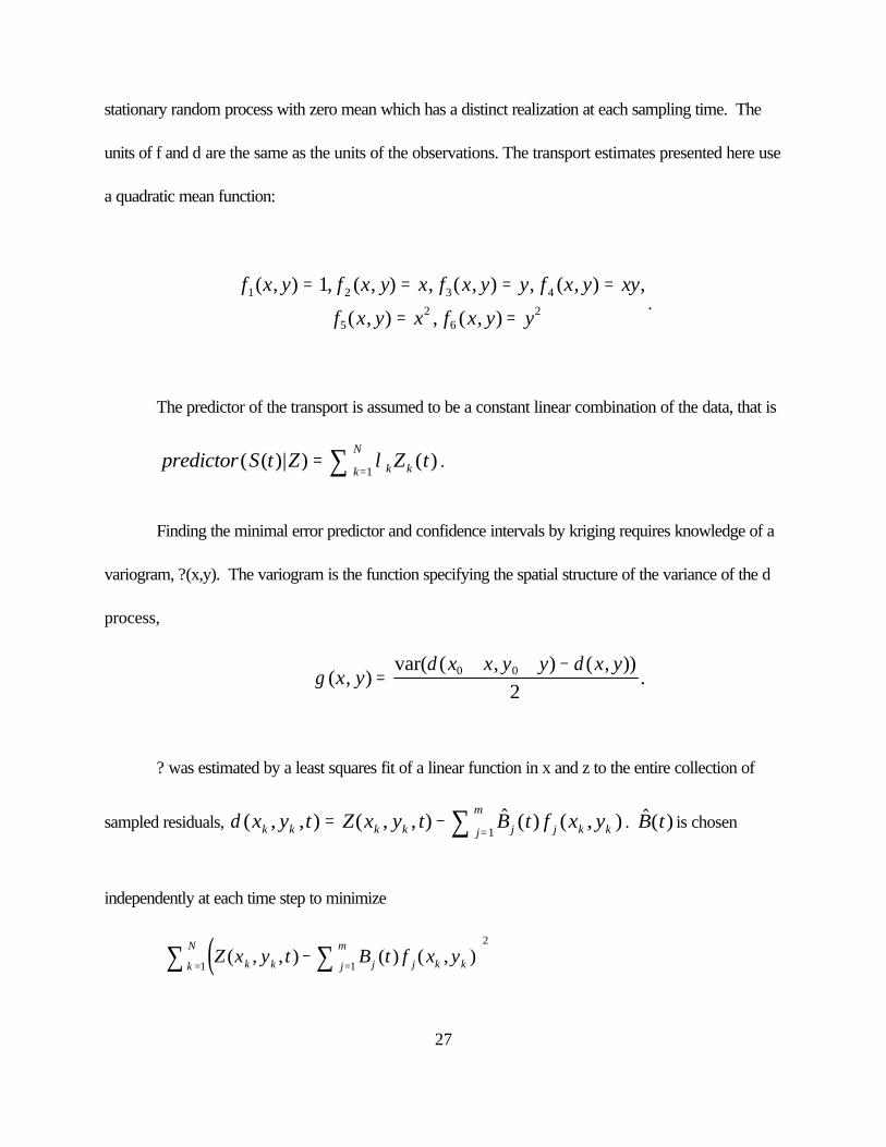
a quadratic mean function:

.f x y f x y x f x y y f x y xy

f x y x f x y y1 2 3 4

52

62

1( , ) , ( , ) , ( , ) , ( , ) ,

( , ) , ( , )

= = = =

= =

The predictor of the transport is assumed to be a constant linear combination of the data, that is

. predictor S t Z Z tk kk

N( ( )| ) ( )=

=∑ λ1

Finding the minimal error predictor and confidence intervals by kriging requires knowledge of a

variogram, ?(x,y). The variogram is the function specifying the spatial structure of the variance of the d

process,

γδ δ

( , )var( ( , ) ( , ))

.x yx x y y x y

=+ + −0 0

2

? was estimated by a least squares fit of a linear function in x and z to the entire collection of

sampled residuals, . is chosenδ ( , , ) ( , , ) $ ( ) ( , )x y t Z x y t B t f x yk k k k j j k kj

m= −

=∑ 1$( )B t

independently at each time step to minimize

( )Z x y t B t f x yk k j j k kj

m

k

N( , , ) ( ) ( , )−

== ∑∑ 1

2

1

28

The confidence intervals for the transport estimates by this method of kriging are based on a

mean-squared error of prediction and an assumption that the transport is drawn from a Gaussian

distribution. Because of the assumption that d does not change in time, the error in prediction is

independent of time and is

( )σ λE kk

N

kE S t Z t21

2= −

=∑[ ( ) ( ) ]

where S(t) is the true transport at time t. From the Gaussian assumption, the two-sided a

confidence interval on the prediction of transport, , is$( ) ( )S t Z tkk

N

k==∑ λ

1

.( )$( ) (( ) / ), $( ) (( ) / )S t N S t NE E+ − + +− −σ α σ α1 11 2 1 2

The details of the calculation of minimal variance ? from the data, the f i and ? can be found in

Cressie (1993), section 3.4. A summary of the parameters estimated for the kriging calculation can be

found in Table A1. Figure A1 shows the results of these calculations.

29

REFERENCES

Allen, A. A. (1995) The determination of slippage of drifters and the leeway of search and rescue

targets using Interocean S4 EMCMs. Proceedings of the IEEE Current Meter Conference 1995.

Beardsley, R. C., W. C. Boicourt, and D. V. Hansen (1976) Physical oceanography of the Middle

Atlantic Bight. In: Middle Atlantic Continental Shelf and the New York Bight, Special Symposium,

2, Limnology and Oceanography, M. Grant Gross, Allen Press, Lawrence, Kansas, 441 pp.

Beardsley, R. C., D. C. Chapman, K. H. Brink, S. R. Ramp, and R. Schlitz (1985) The Nantucket

Shoals Flux Experiment (NSFE79). Part I: A basic description of the current and temperature

variability. Journal of Physical Oceanography, 15, 713-748.

Bendat, J. S. and A. G. Piersol (1986) Random data. J. Wiley and Sons, New York, 566pp.

Butman, B. and R. C. Beardsley (1987) Long-term observations on the southern flank of Georges

Bank. Part I: A description of the seasonal cycle of currents, temperature, stratification, and wind

stress. Journal of Physical Oceanography, 17, 367-384.

Butman, B., J. W. Loder, and R. C. Beardsley (1987) The seasonal mean circulation: observation and

theory. In: Georges Bank R. H. Backus and D. W. Bourne, MIT Press, Cambridge, Massachusetts,

30

593 pp.

Butman, B., R. C. Beardsley, B. Magnell, D. Frye, J. A. Vermersch, R. Schlitz, R. Limeburner, W. R.

Wright, and M. Noble (1982) Recent Observations of the mean circulation on Georges Bank. Journal

of Physical Oceanography, 12, 569-591.

Churchill, J. H. and T. J. Berger (1998) Transport of Middle Atlantic Bight shelf water to the Gulf

Stream near Cape Hatteras. Journal of Geophysical Research, 103, 30605-30621.

Churchill, J. H. and J. P. Manning (1997) Horizontal convergence and dispersion over the southern

flank of Georges Bank, ICES CM 1997/T:31.

Cohen, E. B., D. G. Mountain, and R. G. Lough (1986) Possible factors responsible for the variable

recruitment of the 1981, 1982, and 1983 year-classes of haddock (Melanogrammus aeglefinus L.) on

Georges Bank. Northwest Atlantic Fisheries Organization, SRC. Document 86/110, Serial Number

N1237. 27 pp.

Cressie, N. A. C. (1993) Statistics for spatial data. J. Wiley and Sons, New York, 900pp.

Flagg, C. N. (1987) Hydrographic structure and variability. In: Georges Bank R. H. Backus and D.

W. Bourne, MIT Press, Cambridge, Massachusetts, 593 pp.

31

Flagg, C. N. (1977) The kinematics and dynamics of the New England Continental Shelf and

shelf/slope front. Ph.D. thesis. Woods Hole Oceanographic Institution - Massachusetts Institute of

Technology, WHOI Reference 77-67, Woods Hole, Massachusetts, 208pp.

Flagg, C. N., J. A. Vermersch, and R. C. Beardsley (1976) 1974 MIT New England Shelf Dynamics

Experiment (March 1974) data report, part II: The moored array. MIT Technical Report 76-1,

Massachusetts Institute of Technology, Cambridge, Massachusetts, 22pp.

Garvine, R. W., K. -C. Wong, G. G. Gawarkiewicz, R. K. McCarthy, R. W. Houghton, and F.

Aikman III (1988) The morphology of shelfbreak eddies. Journal of Geophysical Research, 93, C

12, 15,593-15,607.

Geyer, W. R. (1989) Field calibration of mixed-layer drifters. Journal of Atmospheric and Ocean

Technology, 6, 333-342.

Greenberg, D. A., J. W. Loder, Y. Shen, D. R. Lynch, and C. E. Naimie (1997) Spatial and temporal

structure of the barotropic response of the Scotian Shelf and Gulf of Maine to surface wind stress: A

model-based study. Journal of Geophysical Research, 102, 20,897-20,915.

Houghton, R. W., R. Schlitz, R. C. Beardsley, B. Butman, and J. L. Chamberlin (1982) The Middle

Atlantic Cold Pool: Evolution of the temperature structure during summer 1979. Journal of Physical

32

Oceanography, 12, 1019-1029.

Iles, D. and M. Sinclair (1982) Atlantic herring stock discreteness and abundance. Science, 215, 627-

633.

Kennelly, M. A., R. H. Evans, and T. M. Joyce (1985) Small-scale cyclones on the periphery of a Gulf

Stream warm-core ring. Journal of Geophysical Research, 90, C 5, 8,845-8,857.

LeBlanc, P. R. (1986) The distribution and abundance of larval fishes in shelf water entrained by warm-

core ring 82-B. M.S. thesis. Southeast Massachusetts University, South Dartmouth, Massachusetts,

143 pp.

Limeburner, R. and R. C. Beardsley (1996) Near-surface recirculation over Georges Bank. Deep-Sea

Research II, 43, 1547-1574.

Linder, C. A. and G. G. Gawarkiewicz (1998) A climatology of the shelfbreak front in the Middle

Atlantic Bight. Journal of Geophysical Research, 103, 18,405-18,423.

Manning, J. P. and R. C. Beardsley (1996) Assessment of Georges Bank recirculation from Eulerian

current observations in the Great South Channel. Deep-Sea Research II, 43, 1575-1600.

33

Manning, J. P. and G. Strout (2000) Georges Bank Winds: 1975-1997. Deep-Sea Research II,

accepted.

Manning, J. P., R. G. Lough, C. E. Naimie, and J. H. Churchill (1999) The effect of a slope water

intrusion and shelfbreak jet on larval advection along the southern flank of Georges Bank, ICES

Journal of Marine Science, accepted.

Mercier, H. and K. G. Speer (1998) Transport of bottom water in the Romanche Fracture Zone and

the Chain Fracture Zone. Journal of Physical Oceanography, 28, 779-790.

Moody, J. A., B. Butman, R. C. Beardsley, W. S. Brown, P. Daifuku, J. D. Irish, D. A. Mayer, H. O.

Mofjeld, B. Petrie, S. Ramp, P. Smith, and W. R. Wright (1984) Atlas of Tidal Elevation and Current

Observations on the Northeast American Continental Shelf and Slope. U.S. Geological Survey Bulletin

1611, Woods Hole, Massachusetts, 122 pp.

Noble, M., B. Butman, and M. Wimbush (1985) Wind-current coupling on the southern flank of

Georges Bank: Variation with season and frequency. Journal of Physical Oceanography, 15, 604-

620.

Pickart R. S., D. J. Torres, T. K. McKee, M. J. Caruso, and J. E. Przystup (1999) Diagnosing a

meander of the shelfbreak current in the Middle Atlantic Bight. Journal of Geophysical Research,

34

104, 3121-3132.

Ramp, S. R. (1989) Moored observations of current and temperature on the shelf and upper slope near

ring 82B. Journal of Geophysical Research, 94, 18071-18087.

Ramp S. R. (1986) The interaction of warm core rings with the shelf water and shelf/slope front south

of New England. Ph.D. dissertation, University of Rhode Island, Kingston, Rhode Island, 137 pp.

Schlitz, R. J. (1999) The interaction of shelf water with warm-core rings. Journal of Geophysical

Research, in revision.

Schlitz, R. J. and E. B. Cohen (1984) A nitrogen budget for the Gulf of Maine and Georges Bank.

Biological Oceanography. 3, 203-222.

Werner, S. R. (1999) Surface and bottom boundary layer dynamics on a shallow submarine bank:

southern flank of Georges Bank. Ph.D. thesis. Woods Hole Oceanographic Institution - Massachusetts

Institute of Technology, MIT/WHOI Reference 99-13, Woods Hole, Massachusetts, Massachusetts,

222pp.

35

TABLES

Table 1. Basic information for the second array of current meters set as part of the Warm-Core Rings

Experiment (WRCII), 10 August - 25 September, 1982. Panel a. contains the basic statistics on the

time series averaged to hourly samples. Panel b. contains statistics for low-passed data after filtering to

remove tidal and inertial energy.

Table 2. Principal axes and mean values for the data collected as part of WCRII, 10 August - 25

September, 1982. Panel a. has the principal axes of low-passed currents. The direction for the major

axis is arbitrarily chosen to correspond to the highest numerical value on the compass. For example the

major axis for 5-1 is along 080-260E T. Panel b. has the overall mean speed and direction for each

instrument in the array.

Table 3. Data for drifters launched and recovered during a cruise of R/V Albatross IV. Each drifter

was drogued with a window-shade centered at 10 m.

Table 4. Weights used and mean estimates for transport of shelf water by the geometric method and

universal block kriging for WCRII. Panel A. uses the salinity from the CTD section in August, 1982

(Case 1) to determine shelf water and Panel B. uses salinity from the CTD section in September, 1982

(Case 2).

36

Table A1. Coefficients used in the geometric method and universal block kriging for estimating

transport from an array of velocities at individual points. Lambda (?) is the vector of coefficients for

linear estimator of mean transport producing minimum error.

37

FIGURES

Figure 1. AVHRR image taken at 08:00 Z on 16 August 1982 for region south of Georges Bank

showing interactions of the Gulf Stream. Positions of the array set for Warm-Core Rings II (WRCII)

are shown for reference.

Figure 2. Locations for moored array set during Warm-Core Rings II (WRCII), 10 August - 25

September 1982 on southern flank of Georges Bank. Mean low-passed currents from each current

meter and mean velocities from drogues are shown. Mooring locations are circles and launch points for

drogues are squares. The designation at the head of the arrow corresponds to the depth in meters for the

measurement . All drogues are at 10 m. Also shown is the position of NOAA data buoy 44003.

Bathymetry is in meters.

Figure 3. Temperature (EC), salinity (psu), and density (s t) sections across the southern flank of

Georges Bank. Figure 3a. is for data collected on 16 August, 1982 during the cruise on R/V Albatross

IV to set the moored array. Figure 3b. is for data collected on 25 September 1982, during the cruise on

R/V Delaware II to recover the array. Positions of individual instruments are also shown. The black

lines indicate boundaries to areas assigned for transport calculations.

Figure 4. Temperature-Salinity diagram for CTD stations completed in the vicinity of moorings and

drogues during the cruise on R/V Albatross IV.

38

Figure 5. Low-passed temperature records from thermisters on each current meter during WCRII, 10

August - 25 September 1982. Figure 5a. is for records at 10 m depth. Figure 5b. is for all deeper

records.

Figure 6. Progressive vectors for velocities recorded at moorings during WCR II. The top panel is for

records at 10 m depth and the bottom panel is for all deeper records. All velocities were first scaled by

0.1 (i.e. the distance shown is one tenth that which a water parcel would travel) to fit on one chart. Tidal

excursions are shown by cross-shelf variability in the tracks. Note that the depth of each record in the

lower panel is posted in italics at the end of the track. Bathymetry in meters is labeled on the upper

panel.

Figure 7. AVHRR image taken at 08:00 Z on 16 August 1982 showing vectors for each current

measurement at 10 m at the same hour (black), and overall mean velocity for drogues with window-

shades centered at 10 m (blue). The boundary for shelf water can be approximated by the 22EC

isotherm.

Figure 8. Low-passed currents at 10 meters for three sites across the southern flank of Georges Bank

and low-passed wind stress at buoy 44003 for 26 - 27 August 1982. Wind speeds during the period

were highest, > 10 ms-1 , for the period of the array.

Figure 9. Low-passed currents at site 6 for depths of 10 and 85 meters and low-passed wind stress at

39

buoy 44003. Figure 9a. shows three events for which there was upwelling associated with SW winds.

Figures 9 b-d. provide details of the interaction of currents and winds for individual events.

Figure 10. Coherence between wind and current contoured as a function direction of wind and period.

Direction of wind is shown by the arrows. Only significant values of coherence are contoured. The

phase angles (negative for wind leading current) and transfer functions, gain in cms-1Pa-1, correspond to

significant coherence only. The top panel is for the north/south component of current and the bottom

panel for the east/west component of current.

Figure 11. Mean residual velocities for drogues after wind-driven component and slippage was

removed. The mean velocities, with wind-driven component removed, over the same period at 10 m

from the current meters are shown. Included is the mean wind stress for the period. Contoured

temperature at the surface is for AVHRR data at 08:00 Z on 16 August 1982.

Figure 12. The first two empirical orthogonal modes calculated from the low-passed records of

alongbank flow during WCRII, 10 August - 25 September 1982 containing 82% of the variance. Mode

1, 63%, is shown by red arrows and mode 2, 19%, is shown by green arrows.

Figure 13. Amplitudes of the first two empirical orthogonal modes and wind stress during WCRII., 10

August - 25 September 1982. The top panel with mode 1 visually shows partial correlation in response.

The bottom panel with mode 2 shows low correlation except for one event on 25-26 August, 1982

40

which caused a significant response.

Figure 14. Alongshelf transport of shelf water for the period of WCRII, 10 August - 25 September

1982, estimated from the salinity distribution at the beginning of the period, 16 August (Case 1). The

top panel shows estimates of the transport from the east/west component of velocity at each site by a

geometric method and universal block kriging. The bottom panel shows estimates of the transport using

the maximum mean velocity at each instrument and same methods. Confidence intervals at 95% level

are vertical lines.

Figure 15. Alongshelf transport of shelf water for the period of WCRII, 10 August - 25 September

1982, estimated from the salinity distribution at the end of the period, 25 September (Case 2). The top

panel shows estimates of the transport from the east/west component of velocity at each site by a

geometric method and universal block kriging. The bottom panel shows estimates of the transport using

the maximum mean velocity at each instrument and same methods. Confidence intervals at 95% level

are vertical lines.

Figure 16. Comparison of alongshelf transports of shelf water for the period of WCRII, 10 August - 25

September 1982. The top panel contains the four estimates using the geometric method. The bottom

panel has the four estimates using universal block kriging. All estimates are within the confidence limits

of the individual time series as shown in Figures 14 and 15.

41

Figure A1. Time series of transport determined by a geometric method and universal block kriging for

an array of current meters.

a. Basic Statistics

Speed in cms-1Northward speed in cms-1Eastward speed in cms-1Temperature in 0CInstrument DepthWater Depth LongitudeLatitudeSitest. devmaximumminimummeanst. devmaximumminimummeanst. dev.maximumminimummeanst. dev.maximumminimummeanmetersmetersWN

12.172.90.524.518.557.9-59.80.119.555.2-72.74.92.224.715.920.11033768 49.340 06.91-111.368.50.121.515.647.7-64-2.217.447.8-68.5-6.1225.216.820.21032567 56.540 18.02-18.247.80.515.813.335.8-44.51.211.633.1-46.7-2.32.2208.5144032367 33.140 22.23-26.5440.515.410.528.4-29.60.810.424.2-40.6-7.70.414.39.712.91003-35.435.90.4107.324.2-35.9-0.97.714-30.1-40.69.35.66.73053-4

15.5100.21.249.938.667.5-98.2-6.832.465.3-78.4-12.20.817.412.915106067 42.840 57.25-118.589.70.643.631.161.9-77.8-92438.1-89.5-252.122.710.617.41010067 35.540 34.96-115.585.80.33626.756.4-69-4.621.631.6-79.3-18.42.220.97.810.9356-2

957.91.628.221.445.4-54.5-2.819.437.6-47.5-5.71.113.38.110.8856-311.481.60.220.717.342.7-73.70.81671.2-49.301.123.41520.11089567 31.640 19.57-1

b. Low-Passed Statistics

Northward speed in cms-1Eastward speed in cms-1Temperature in 0CInstrument DepthWater Depth LongitudeLatitudeSitest. devmaximumminimummeanst. dev.maximumminimummeanst. dev.maximumminimummeanmetersmetersWN

4.412-15.40.27.318.1-12.45224.716.920.11033768 49.340 06.91-14.58.3-20.3-2.28.311.1-31.7-6.71.92517.620.11032567 56.540 18.02-14.811-8.90.94.87-15.6-2.6217.39.614.14032367 33.140 22.23-23.78-10.50.65.47.2-24.7-8.50.313.51212.91003-312.6-3.6-0.95.79.1-21.4-4.20.47.666.73053-4

5.66.2-31-6.86.21.1-27.5-12.50.616.113.515106067 42.840 57.25-18.111-30.6-9.17.4-8.3-46.3-25.31.821.414.417.61010067 35.540 34.96-16.111.6-23.7-56-4.7-33.3-18.61.415811356-22.95.7-9.5-2.85.29.7-17.7-5.80.912.98.910.9856-37.917.3-29.40.96.824.8-16-0.70.922.816.720.11089567 31.640 19.57-1

a. Principal Axes

Principal Axes of the low-passed (PL33) time seriesInstrument DepthWater Depth LongitudeLatitudeSiteangle compassminormajormetersmetersWN

notation: °Taxisaxishighest anglecms-1cms-1

2744.57.41033768 49.340 06.91-1 2784.38.31032567 56.540 18.02-1 2134.754032367 33.140 22.23-2 2412.761003-3 2670.95.73053-4 2605.66.2106067 42.840 57.25-1 3215.69.41010067 35.540 34.96-1 3265.86.2356-2 2542.75.5856-3 3526.96.91089567 31.640 19.57-1

b. Mean Speed and Direction

Mean speed and direction Instrument DepthWater Depth LongitudeLatitudeSite° Tcms-1metersmetersWN

8951033768 49.340 06.91-12537.11032567 56.540 18.02-12892.84032367 33.140 22.23-22748.61003-32584.33053-424214.2106067 42.840 57.25-125026.91010067 35.540 34.96-125519.2356-22446.4856-332611089567 31.640 19.57-1

Launch DepthBearing Mean Drift Overall Distance End Begin Location of Recovery Location of LaunchDrifterMDeg Tcms-1knotsKMNMTime (Z)DateTime (Z)DateLongitudeLatitudeLongitudeLatitudeNumber

2070192.150.045.122.76144216-Aug-82203813-Aug-8267o 09.94'40o 33.34'67o 11.16'40o 30.74'D12050683.670.071.991.07141014-Aug-82231313-Aug-8267o 01.91'40o 39.95'67o 03.22'40o 39.55'D2

15462236.860.1317.419.40184317-Aug-82202114-Aug-8267o 25.71'40o 13.45'67o 17.38'40o 20.37'D35870693.480.074.392.37065017-Aug-82200815-Aug-8267o 13.85'40o 26.45'67o 16.75'40o 25.59'D4

17241453.480.072.381.28202217-Aug-82011017-Aug-8267o 29.89'40o 08.41'67o 30.84'40o 09.47'D5

Summary of measurements for drogued drifters during Albatross IV 82-09

a. Case 1, August 1982

Universal Block KrigingGeometric MethodRecordComponent of VelocityComponent of Velocityfor

Mean DirectionWestMean DirectionWestComputation

0.45280.42830.52500.52505-10.13900.25620.15240.15246-10.32830.24460.16600.16606-20.23780.26570.00420.00426-3-0.1579-0.19480.15240.15247-10.93300.92750.73020.6651Mean Transport (sv)0.22550.20640.18230.176795% Confidence Interval (sv)

b. Case 2, September 1982

Universal Block KrigingGeometric MethodRecordComponent of VelocityComponent of Velocityfor

Mean DirectionWestMean DirectionWestComputation

0.46320.44360.50360.50355-10.17290.27530.13190.13196-10.30940.22960.21080.21086-20.15240.17900.04850.04856-3-0.0980-0.12750.10520.10527-10.88710.86880.83710.7652Mean Transport (sv)0.19910.18520.20340.197295% Confidence Interval (sv)

0.83± 0.2Overall Mean Transport (sv)

Estimate ofRatio of areas NeighborhoodLambda ( λ)Instrumentstandardto total areafor westwarddeviationfor geometrictransport

estimate(kriging)

0.0900.083{3-2, 3-3, 6-1, 7-1}-0.1043-20.0530.157{3-2, 3-3, 3-4, 6-3, 7-1}0.3283-30.0550.139{3-2, 3-3, 6-3, 7-1}0.1233-40.0740.213{5-1, 6-1, 6-2}0.2335-10.1030.062{3-2, 5-1, 6-1, 6-2, 7-1}-0.2706-10.1000.103{3-2, 5-1, 6-1, 6-2, 6-3}0.3176-20.0710.110{3-3, 5-1, 6-2, 6-3}0.2406-30.0530.135{3-2, 3-3, 3-4, 7-1}0.1347-1

10 13 16 19 22 25 28

71 W 70 W 69 W 68 W 67 W

37 N

38 N

39 N

40 N

41 N

42 N

Longitude

Latit

ude

16 August 1982 at 0800Z

60m

100m

200m

Meandering Gulf S

tream

1

23

5

6

7

69 W 68 W 67 W 40 N

41 N

42 N

60

60

60

60

60

60

80

80

80

80

100

100

100

200

200

1000

Longitude

Latit

ude

Nantucket S

hoals

44003

Georges Bank5 cm/s

10

10

40100

305

10

10

35

85

1

2333

5

666

7

1

2

3

4

5

0.005 Pa

1

23

5

6

7

10

−100

−80

−60

−40

−20

0

10 10

1212 12

12

12

12

14 14

16

16 18

44 43 42 41 40 39

Temperature

AL8209 Cross−Bank CTD Transect

3

3

3

5 6

6

6

7

−100

−80

−60

−40

−20

0

32.533

33

33.5

33.5

33.5

34

34

34.5

35

44 43 42 41 40 39

Salinity

3

3

5 6

6

6

7

0 10 20 30 40 50 60 70 80 90−100

−80

−60

−40

−20

023.5 23.5

2424

2424.5 24.52525

25.5

25.5

25.5

26

26

26.5

26.5

44 43 42 41 40 39

Along Track Distance (km) Relative to Northern Most Station

Dep

th (

m)

Density

3

3

5 6

6

6

7

−100

−80

−60

−40

−20

0

8

9910

10 11

11

11

12

12

1212

13

13 131414

14

1515

1616

17

4 10 9 5 8 7 6

Temperature

De8206 Cross−Bank CTD Transect

3

3

3

5 6

6

6

7

−100

−80

−60

−40

−20

0

33

33

3333

33.5

33.5

34

34

34.5

4 10 9 5 8 7 6

Salinity

3

3

5 6

6

6

7

0 10 20 30 40 50 60 70−100

−80

−60

−40

−20

0

2424

24 24.524.5

25

25

25.525.5

25.5

26

26

26.5

4 10 9 5 8 7 6

Along Track Distance (km) Relative to Northern Most Station

Dep

th (

m)

Density

3

3

5 6

6

6

7

32 32.5 33 33.5 34 34.5 35 35.5 36 36.50

5

10

15

20

25

30

Salinity in psu

Tem

pera

ture

in d

eg. C

T−S diagram from CTD data during Ablatross IV cruise AL−8209

09 11 13 15 17 19 21 23 25 27 29 31 02 04 06 08 10 12 14 16 18 20 22 24 2612

14

16

18

20

22

24

26

Tem

pera

ture

in d

eg. C

August September 1982

Temperatures at 10 m from current meters during WCR II

site 1site 2site 5site 6site 7

11 13 15 17 19 21 23 25 27 29 31 02 04 06 08 10 12 14 16 18 20 22 24 264

6

8

10

12

14

16

18

Tem

pera

ture

in d

eg. C

August September 1982

Temperatures at depths greater than 10 m from current meters during WCR II

site 3−2site 3−3site 3−4site 6−2site 6−3

40 N

40 30’N

41 N

Lat

itude

Advection at 10m

1

2

5

6

7

69 W 68 30’W 68 W 67 30’W 40 N

40 30’N

41 N

Longitude

Lat

itude

40m100m

305m

35m

85m

Advection greater than 10m

3

6

100m

200m

2000m

SST image for 8−16−1982 at 0800

Low−passed currents and wind stress during WCRII array, August−September, 1982, including drogues

73oW 72oW 71oW 70oW 69oW 68oW 67oW 66oW 38oN

39oN

40oN

41oN

42oN

16

16

16

16

16

16

16

18

18

18

18 18

1818

18

20

20

202020

20

20

22

22

22

2222

22

22

24

24

24

24

24

26

26

2626

26

26

26

26

26

73oW 72oW 71oW 70oW 69oW 68oW 67oW 66oW 38oN

39oN

40oN

41oN

42oN

60

60 60

60

80

80

80

80

80

100

100

100 100

100

200

200

200

200

500

500

500

10001000

1000

25 cm/sec

0.1 pascal

D1 D2

D3 D4

D5

0 5 10 15 20 25

25

August 82

26

−20

−10

0

10 7−1 10m

cm/s

−20

−10

0

106−1 10m

cm/s

−20

−10

0

10 5−1 10m

cm/s

−0.02

0.00

0.02

0.04 Wind Stress

Pa

27

19

August 82

29 8

September 82

−10

−5

0

5 6−3 85m

cm/s

−30

−20

−10

0

10 6−1 10m

cm/s

−0.04

−0.02

0.00

0.02

0.04

0.06 Wind Stress

Pa

1 2 3

25

August 82

26

−20

−10

0

10 6−3 85m

cm/s

−20

−10

0

10 6−1 10m

cm/s

−0.02

0.00

0.02

0.04 Wind Stress

Pa

27

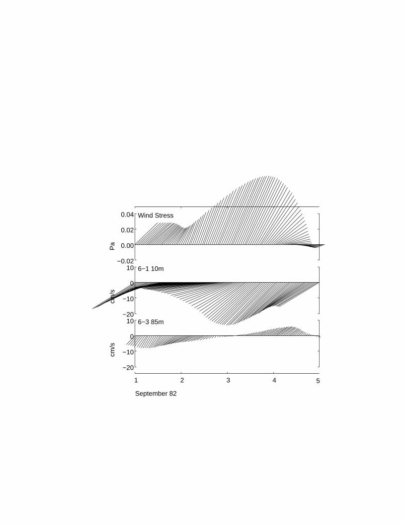
1

September 82

2 3 4

−20

−10

0

10 6−3 85m

cm/s

−20

−10

0

10 6−1 10m

cm/s

−0.02

0.00

0.02

0.04 Wind Stress

Pa

5

9

September 82

10 11

−20

−10

0

10 6−3 85m

cm/s

−20

−10

0

10 6−1 10m

cm/s

−0.02

0.00

0.02

0.04 Wind Stress

Pa

0.5

0.54

0.58

0.62

0.66

0.7

0.74

20

40

60

80

100

120Rotated−East/West Wind Driving North/South Current

Per

iod

(hou

rs)

234139

233150

237159

246167

259173

275179

292−174

303−165

GainPhase

0.5

0.54

0.58

−80 −60 −40 −20 0 20 40 60 8020

40

60

80

100

120Rotated−North/South Wind Driving East/West Current

Per

iod

(hou

rs)

160−13.9

145−13.6

136−13.2

133−12.8

135−12.5

GainPhase

Wind Angle (Clockwise Rotation)

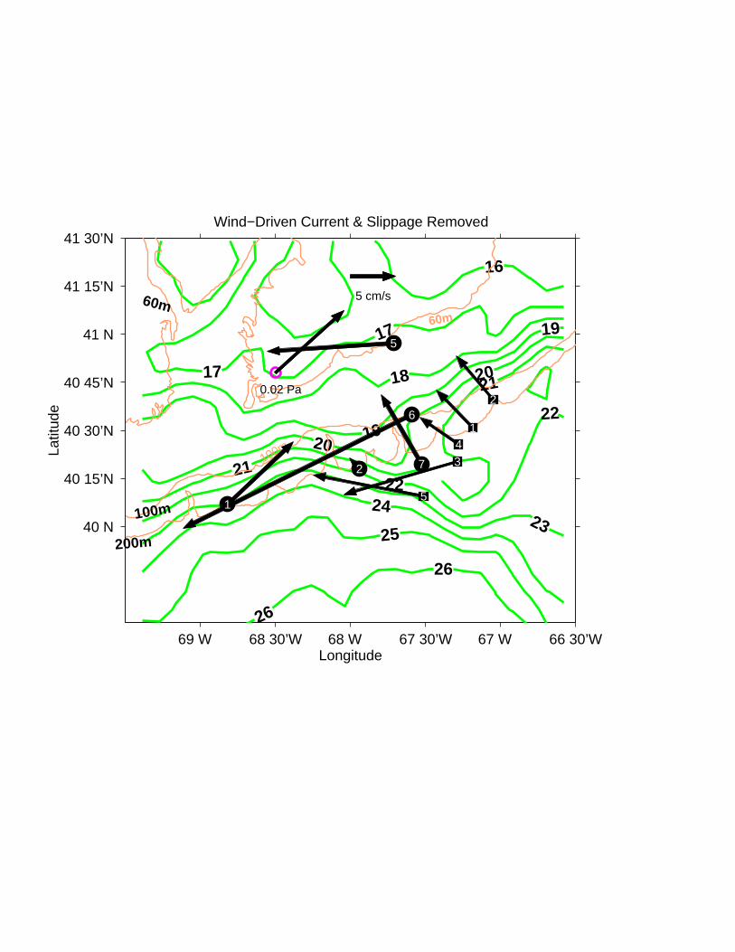
69 W 68 30’W 68 W 67 30’W 67 W 66 30’W

40 N

40 15’N

40 30’N

40 45’N

41 N

41 15’N

41 30’N

16

17

17

18

19

19

20

20

21

21

22

22

2324

25

26

26

Longitude

Latit

ude

100m

60m

Wind−Driven Current & Slippage Removed

60m

100m

200m

5 cm/s

1

2

5

6

7

1

2

34

5

0.02 Pa

−69

−68.5

−68

−67.5

−67

40

40.5

41

41.5

42−100

−80

−60

−40

−20

0

7

3

6

Longitude

5

80m

Mode 1 (red) and 2 (green)

60m

Latitude

Dep

th(m

)

100m

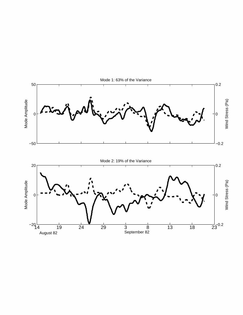
−50

0

50

Mod

e A

mpl

itude

Mode 1: 63% of the Variance

−0.2

0

0.2

Win

d S

tres

s (P

a)−20

0

20

Mod

e A

mpl

itude

Mode 2: 19% of the Variance

August 82 September 8214 19 24 29 3 8 13 18 23

−0.2

0

0.2

Win

d S

tres

s (P

a)

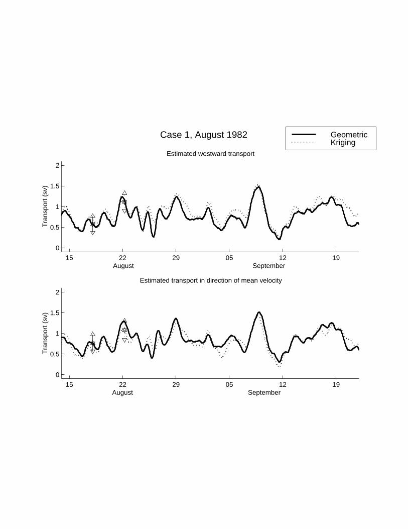
15 22 29 05 12 19

0

0.5

1

1.5

2

Estimated transport in direction of mean velocity

Tra

nspo

rt (

sv)

August September

GeometricKriging

Case 1, August 1982

15 22 29 05 12 19

0

0.5

1

1.5

2

Estimated westward transport

August September

Tra

nspo

rt (

sv)

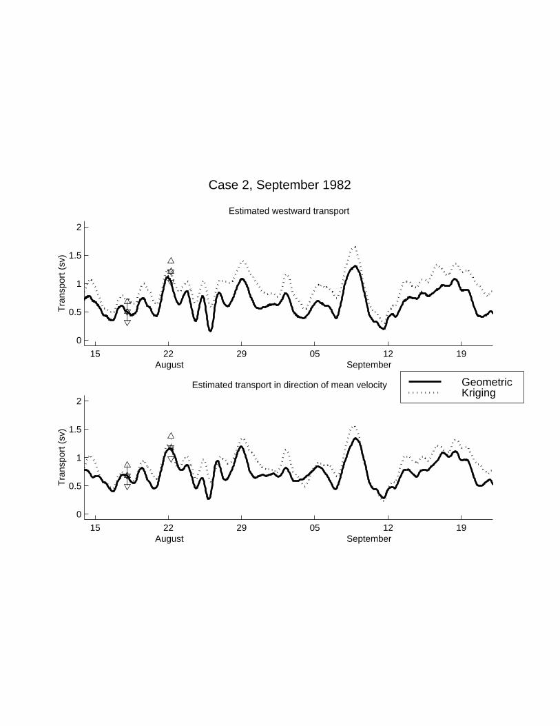
15 22 29 05 12 19

0

0.5

1

1.5

2

Estimated transport in direction of mean velocity

August September

Tra

nspo

rt (

sv)

GeometricKriging

Case 2, September 1982

15 22 29 05 12 19

0

0.5

1

1.5

2

Estimated westward transport

August September

Tra

nspo

rt (

sv)

12 17 22 27 01 06 11 16 21 26

0

0.5

1

1.5

2Transport estimated by geometric method

Tra

nspo

rt (

sv)

August September

12 17 22 27 01 06 11 16 21 26

0

0.5

1

1.5

2Transport estimated by Kriging

Tra

nspo

rt (

sv)

August September

West−case 2Mean−case 2West−case 1Mean−case 1

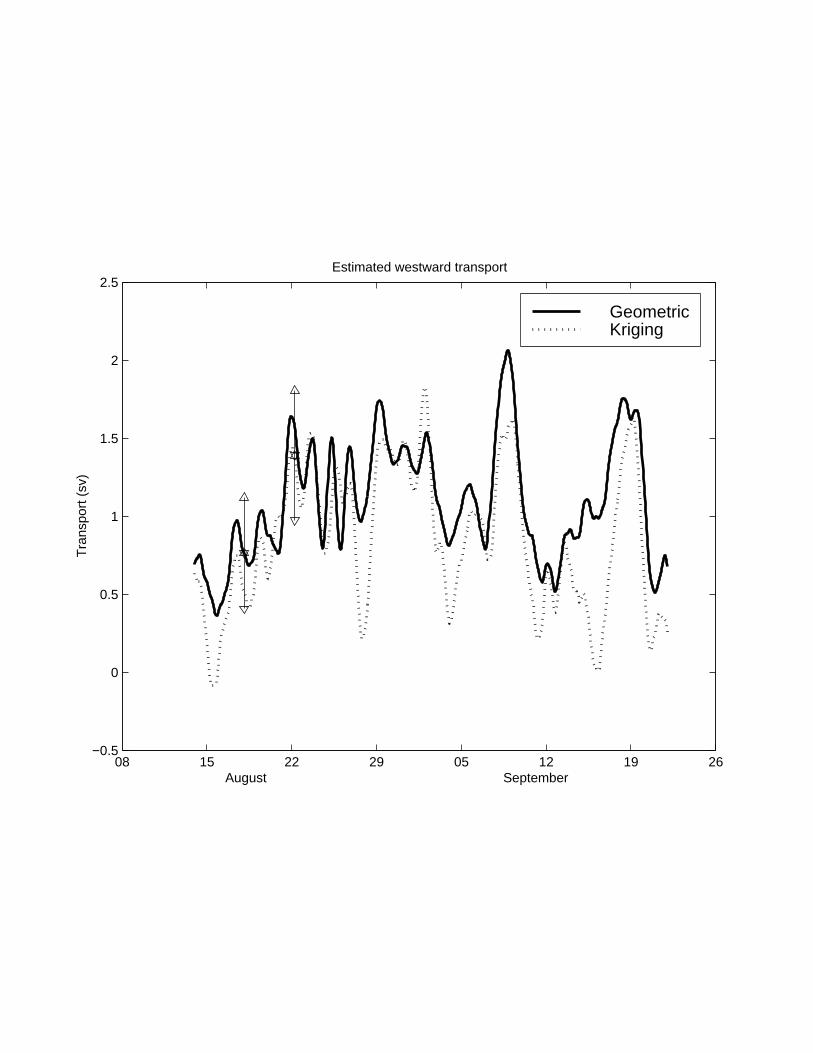
08 15 22 29 05 12 19 26−0.5

0

0.5

1

1.5

2

2.5Estimated westward transport

Tra

nspo

rt (

sv)

August September

GeometricKriging