Structure factor statistics and likelihood

Randy J Read

Principle of maximum likelihood

•  Best model is most consistent with data •  Measure consistency by probabilities •  Optimise model by adjusting parameters in

probability distribution

•  Crystallographic likelihood is based on probability distributions of structure factors •  univariate for maps, molecular replacement, refinement •  multivariate for experimental phasing and other advanced

applications

Wilson distribution

Structure factors with random atoms

•  Assume atoms randomly scattered relative to Bragg planes

•  Random walk in complex plane

The Central Limit Theorem

•  Probability distribution of a sum of independent random variables tends to be Gaussian •  regardless of distributions of variables in sum

•  Conditions: •  sufficient number of independent random variables •  none may dominate the distribution

•  Centroid (mean) of Gaussian is sum of centroids •  Variance of Gaussian is sum of variances

Wilson distribution for space group P1

•  Apply central limit theorem to real and imaginary parts of structure factor separately •  sums of real and imaginary atomic contributions

Derivation of Wilson distribution: centroids

F = f j exp 2πih ⋅x j( )j=1

Natom

∑ = f j cos 2π h ⋅x j( )j=1

Natom

∑ + i f j sin 2π h ⋅x j( )j=1

Natom

∑= A + iB

F = A + iB = A + i B

A = f j cos 2π h ⋅x j( )j=1

Natom

∑= 0, (assume random position relative to Bragg planes)

B = f j sin 2π h ⋅ x j( )j=1

Natom

∑ = 0

F = 0

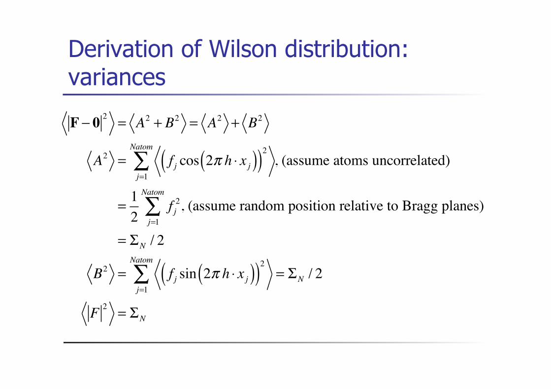
Derivation of Wilson distribution: variances

F − 0 2 = A2 + B2 = A2 + B2

A2 = f j cos 2π h ⋅ x j( )( )2

j=1

Natom

∑ , (assume atoms uncorrelated)

= 12

f j2

j=1

Natom

∑ , (assume random position relative to Bragg planes)

= ΣN / 2

B2 = f j sin 2π h ⋅ x j( )( )2

j=1

Natom

∑ = ΣN / 2

F 2 = ΣN

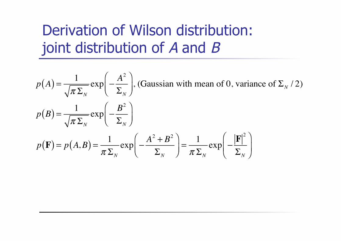
Derivation of Wilson distribution: joint distribution of A and B

p A( ) = 1π ΣN

exp − A2

ΣN

⎛⎝⎜

⎞⎠⎟

, (Gaussian with mean of 0, variance of ΣN / 2)

p B( ) = 1π ΣN

exp − B2

ΣN

⎛⎝⎜

⎞⎠⎟

p F( ) = p A,B( ) = 1π ΣN

exp − A2 + B2

ΣN

⎛⎝⎜

⎞⎠⎟= 1π ΣN

exp −F 2

ΣN

⎛

⎝⎜⎞

⎠⎟

Alternative derivation of Wilson distribution

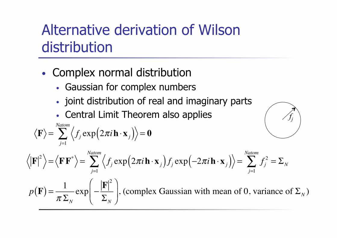
•  Complex normal distribution •  Gaussian for complex numbers •  joint distribution of real and imaginary parts •  Central Limit Theorem also applies

F = f j exp 2πih ⋅x j( )j=1

Natom

∑ = 0

F 2 = FF* = f j exp 2πih ⋅x j( ) f j exp −2πih ⋅x j( )j=1

Natom

∑ = f j2

j=1

Natom

∑ = ΣN

p F( ) = 1π ΣN

exp −F 2

ΣN

⎛

⎝⎜⎞

⎠⎟, (complex Gaussian with mean of 0, variance of ΣN )

fj

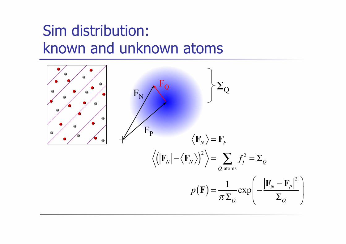
Sim distribution: known and unknown atoms

FP

FQ FN

ΣQ

FN = FP

FN − FN( )2= f j

2

Q atoms∑ = ΣQ

p F( ) = 1π ΣQ

exp −FN −FP

2

ΣQ

⎛

⎝⎜

⎞

⎠⎟

Sim distribution for amplitudes

•  Likelihood function is the probability of the observations •  but only the intensity (or amplitude) is measured •  phase component has to be eliminated

•  Change variables from real and imaginary to amplitude and phase

•  Integrate over all possible values of (unknown) phase

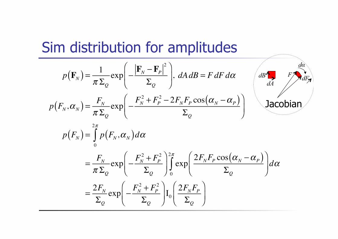
Sim distribution for amplitudes

p FN( ) = 1π ΣQ

exp −FN −FP

2

ΣQ

⎛

⎝⎜

⎞

⎠⎟ , dAdB = F dF dα

p FN ,αN( ) = FNπ ΣQ

exp −FN

2 + FP2 − 2FNFP cos αN −αP( )

ΣQ

⎛

⎝⎜⎞

⎠⎟

p FN( ) = p FN ,αN( )dα0

2π

∫

= FNπ ΣQ

exp − FN2 + FP

2

ΣQ

⎛

⎝⎜⎞

⎠⎟exp

2FNFP cos αN −αP( )ΣQ

⎛

⎝⎜⎞

⎠⎟dα

0

2π

∫

= 2FNΣQ

exp − FN2 + FP

2

ΣQ

⎛

⎝⎜⎞

⎠⎟I0

2FNFPΣQ

⎛

⎝⎜⎞

⎠⎟

dA dB dF

dα F

Jacobian

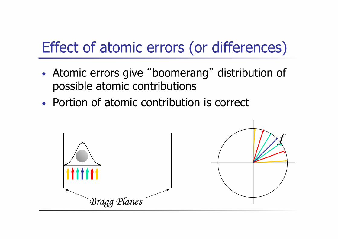
Effect of atomic errors (or differences)

•  Atomic errors give “boomerang” distribution of possible atomic contributions

•  Portion of atomic contribution is correct

f

Bragg Planes

df

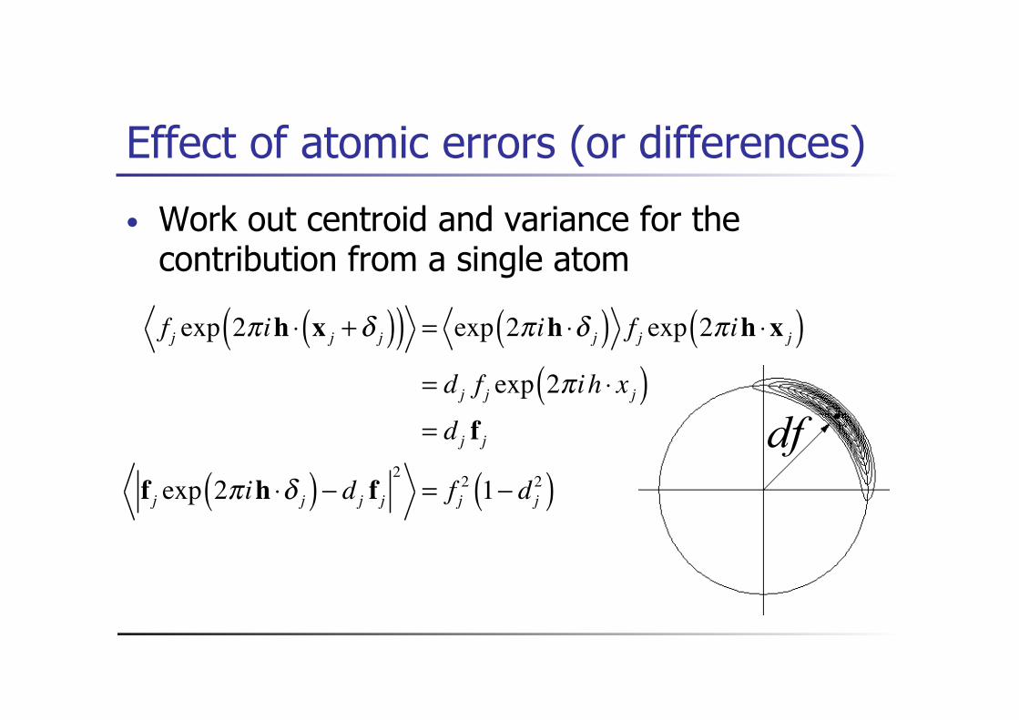
Effect of atomic errors (or differences)

•  Work out centroid and variance for the contribution from a single atom

f j exp 2πih ⋅ x j +δ j( )( ) = exp 2πih ⋅δ j( ) f j exp 2πih ⋅x j( )= dj f j exp 2πih ⋅ x j( )= dj f j

f j exp 2πih ⋅δ j( )− dj f j 2 = f j2 1− dj

2( )

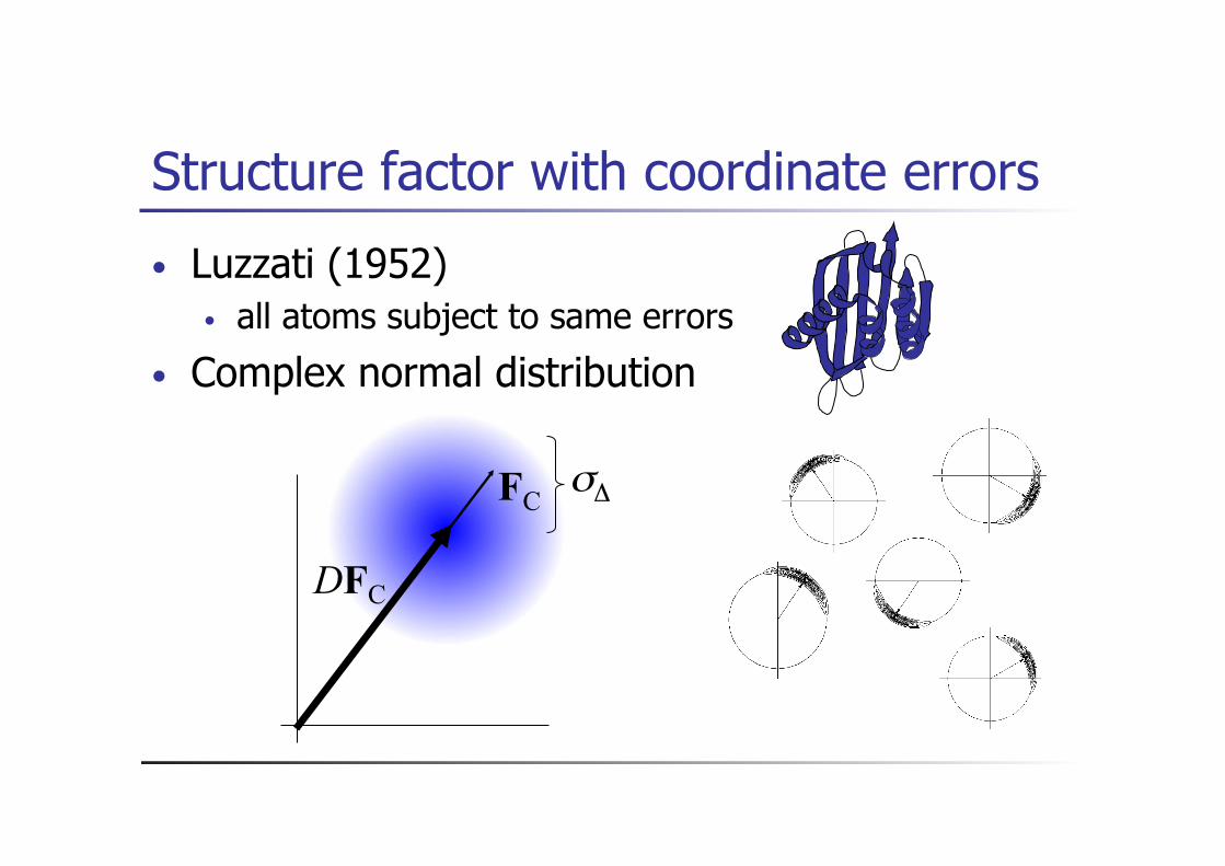
Structure factor with coordinate errors

•  Luzzati (1952) •  all atoms subject to same errors

•  Complex normal distribution

DFC

FC σΔ

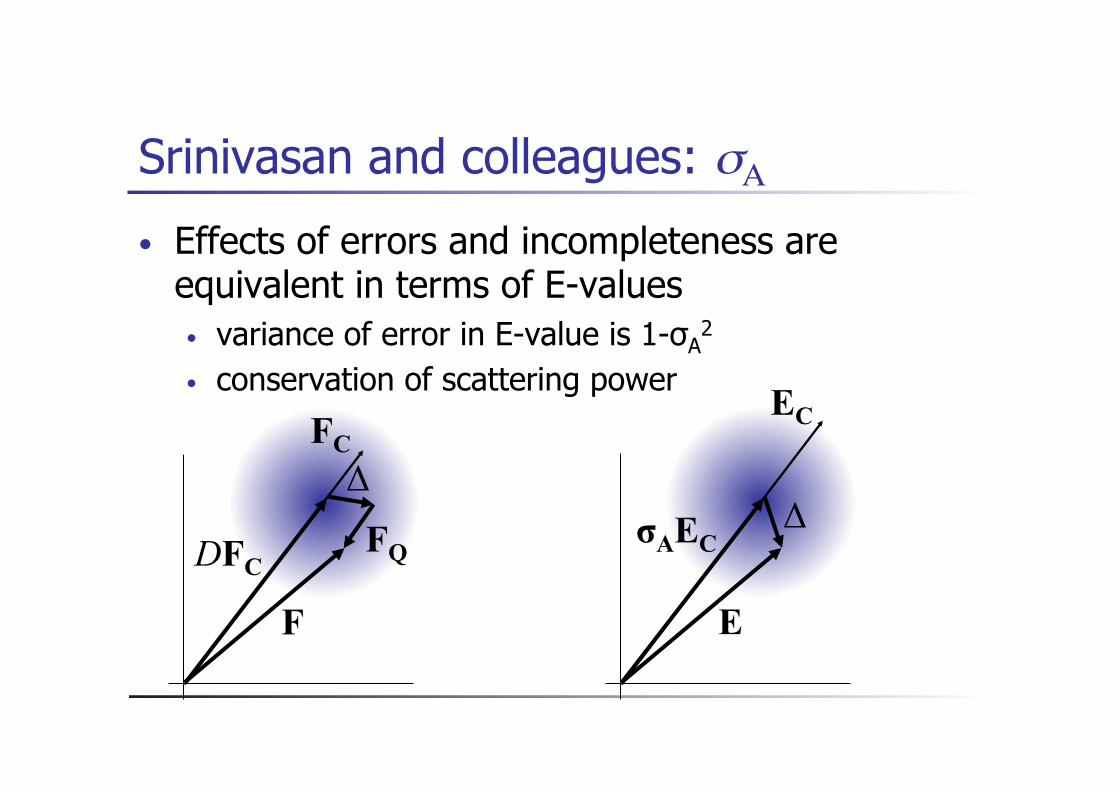
Srinivasan and colleagues: σΑ

•  Effects of errors and incompleteness are equivalent in terms of E-values •  variance of error in E-value is 1-σA

2

•  conservation of scattering power

DFC

FC Δ

F

FQ σAEC

EC

Δ

E

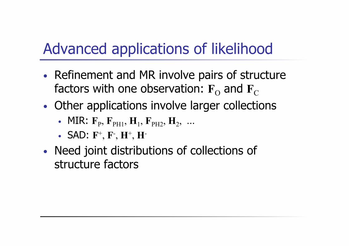
Advanced applications of likelihood

•  Refinement and MR involve pairs of structure factors with one observation: FO and FC

•  Other applications involve larger collections •  MIR: FP, FPH1, H1, FPH2, H2, … •  SAD: F+, F-, H+, H-

•  Need joint distributions of collections of structure factors

Likelihood for more structure factors

•  σΑ can be interpreted as complex covariance between normalised structure factors

•  New applications based on multivariate complex normal distribution •  difficulty is integrating out more than one phase! •  can always isolate one phase by factoring probability

distribution •  see paper on SAD likelihood target

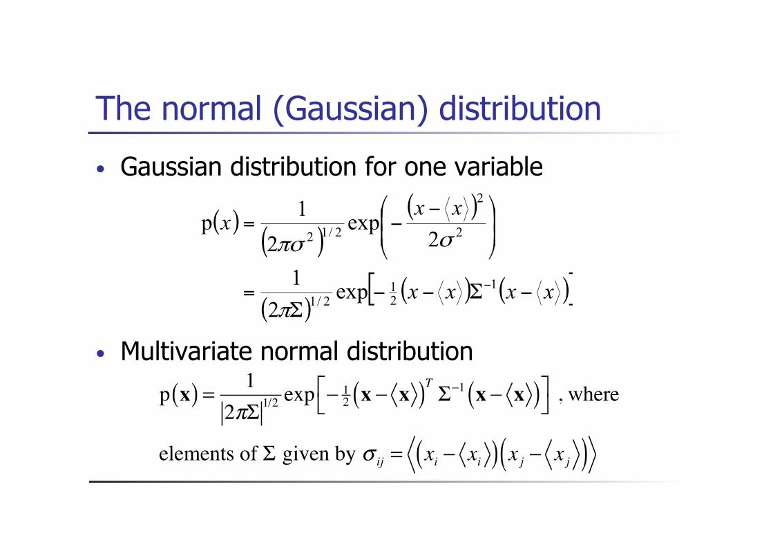
The normal (Gaussian) distribution

•  Gaussian distribution for one variable

•  Multivariate normal distribution

( )( )

( )

( )( ) ( )[ ]xxxx

xxx

−Σ−−Σ

=

⎟⎟⎠

⎞⎜⎜⎝

⎛ −−=

−121

2/1

2

2

2/12

exp21

2exp

21p

π

σπσ

p x( ) = 12πΣ 1/2 exp − 1

2 x − x( )T Σ−1 x − x( )⎡⎣

⎤⎦ , where

elements of Σ given by σ ij = xi − xi( ) x j − x j( )

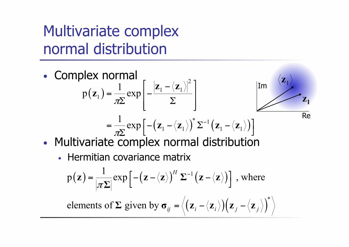
Multivariate complex normal distribution

•  Complex normal

•  Multivariate complex normal distribution •  Hermitian covariance matrix

( ) ( ) ( )

( )( )

1

*

1p exp , where

elements of given by

H

ij i i j j

π−⎡ ⎤= − − −⎣ ⎦

= − −

z z z Σ z zΣ

Σ σ z z z z

( )

( ) ( )

21 1

1

* 11 1 1 1

1p exp

1 exp

π

π−

⎡ ⎤−= −⎢ ⎥

Σ Σ⎢ ⎥⎣ ⎦

⎡ ⎤= − − Σ −⎣ ⎦Σ

z zz

z z z z

1z

Re

Im

z1

•  Start with large joint distribution

•  Fix known or model (y) terms •  partition covariance matrix

•  update covariances and expected values for remaining variables

Deriving conditional Gaussian probability

data − data data −modeldata −model model −model

⎡

⎣⎢

⎤

⎦⎥ =

Σ11 Σ12Σ21 Σ22

⎡

⎣⎢⎢

⎤

⎦⎥⎥

x1xm

⎡

⎣

⎢⎢⎢⎢

⎤

⎦

⎥⎥⎥⎥

= Σ12Σ22−1

y1yn

⎡

⎣

⎢⎢⎢⎢

⎤

⎦

⎥⎥⎥⎥

p x1,x2 ,…,xm , y1, y2 ,… yn( )

Σ11' = Σ11 − Σ12Σ22

−1Σ21

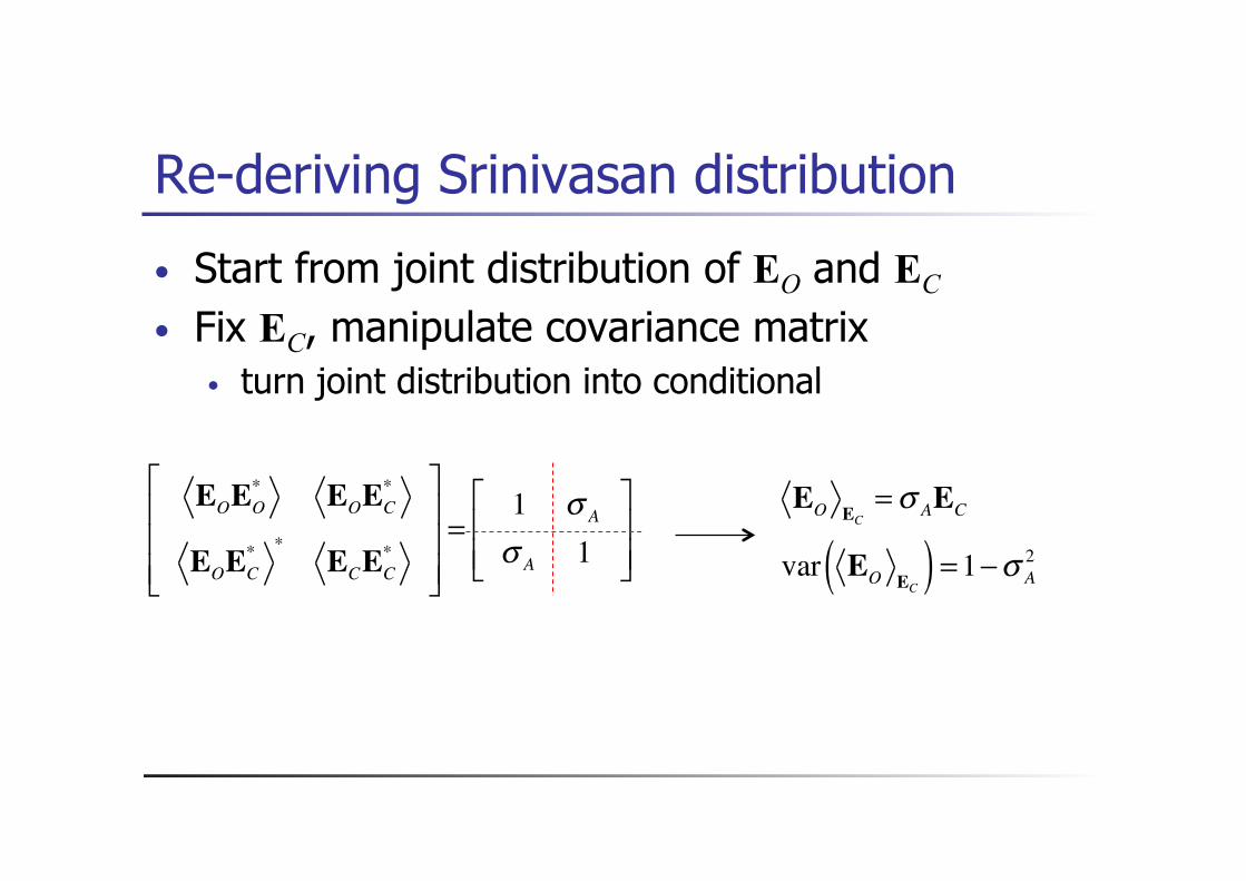
Re-deriving Srinivasan distribution

•  Start from joint distribution of EO and EC •  Fix EC, manipulate covariance matrix

•  turn joint distribution into conditional

EOEO* EOEC

*

EOEC* *

ECEC*

⎡

⎣

⎢⎢⎢

⎤

⎦

⎥⎥⎥=

1 σ A

σ A 1

⎡

⎣⎢⎢

⎤

⎦⎥⎥

EO EC=σ AEC

var EO EC( ) =1−σ A2

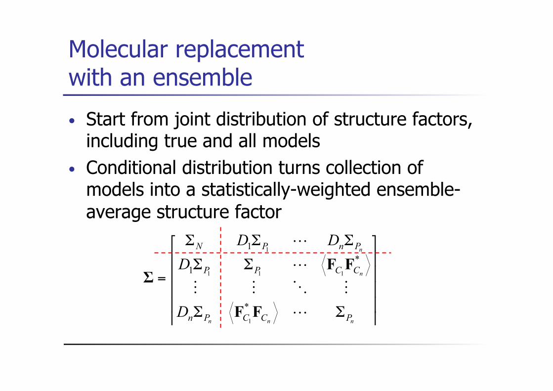
Molecular replacement with an ensemble

•  Start from joint distribution of structure factors, including true and all models

•  Conditional distribution turns collection of models into a statistically-weighted ensemble-average structure factor

⎥⎥⎥⎥

⎦

⎤

⎢⎢⎢⎢

⎣

⎡

ΣΣ

ΣΣ

ΣΣΣ

=

nnn

n

n

PCCPn

CCPP

PnPN

D

DDD

FF

FFΣ

*

*1

1

1

111

1

SAD: probabilities for Friedel pair

•  Start from joint distribution of true and calculated structure factors

•  Use standard manipulations to get conditional probability:

ΣN FO+FO

− FO+H+* FO

+H−

FO+FO

− *ΣN FO

−H+ *FO

−*H−

FO+*H+ FO

−H+ ΣH H+H−

FO+H− *

FO−H−* H+H− *

ΣH

⎡

⎣

⎢⎢⎢⎢⎢⎢⎢

⎤

⎦

⎥⎥⎥⎥⎥⎥⎥

p FO+ ,FO

− ,H+ ,H−( )→ p FO+ ,FO

−;H+ ,H−( )

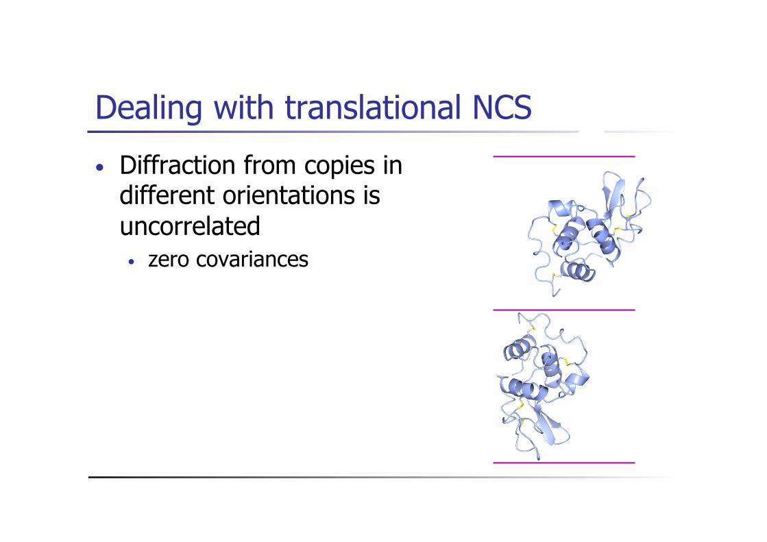
Dealing with translational NCS

•  Diffraction from copies in different orientations is uncorrelated •  zero covariances

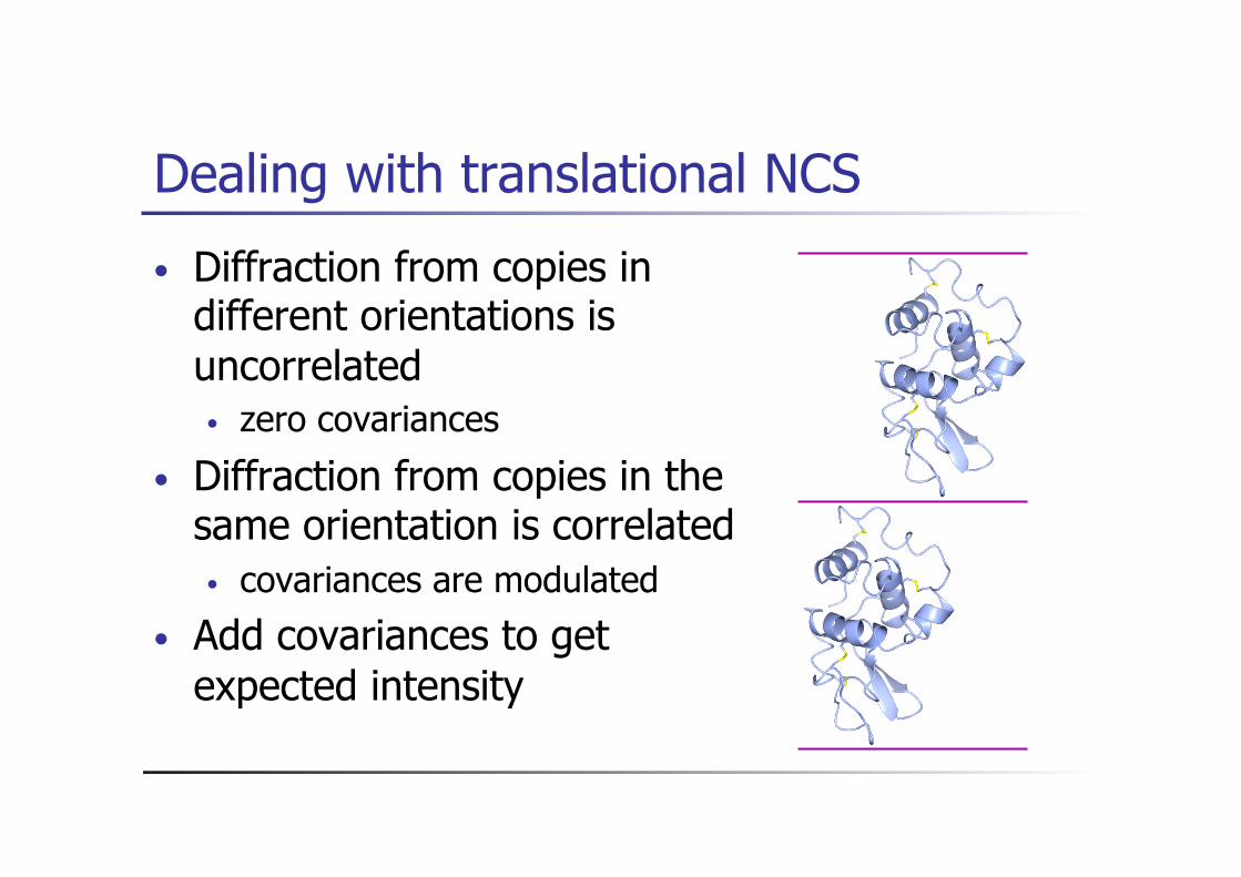
Dealing with translational NCS

•  Diffraction from copies in different orientations is uncorrelated •  zero covariances

•  Diffraction from copies in the same orientation is correlated •  covariances are modulated

•  Add covariances to get expected intensity

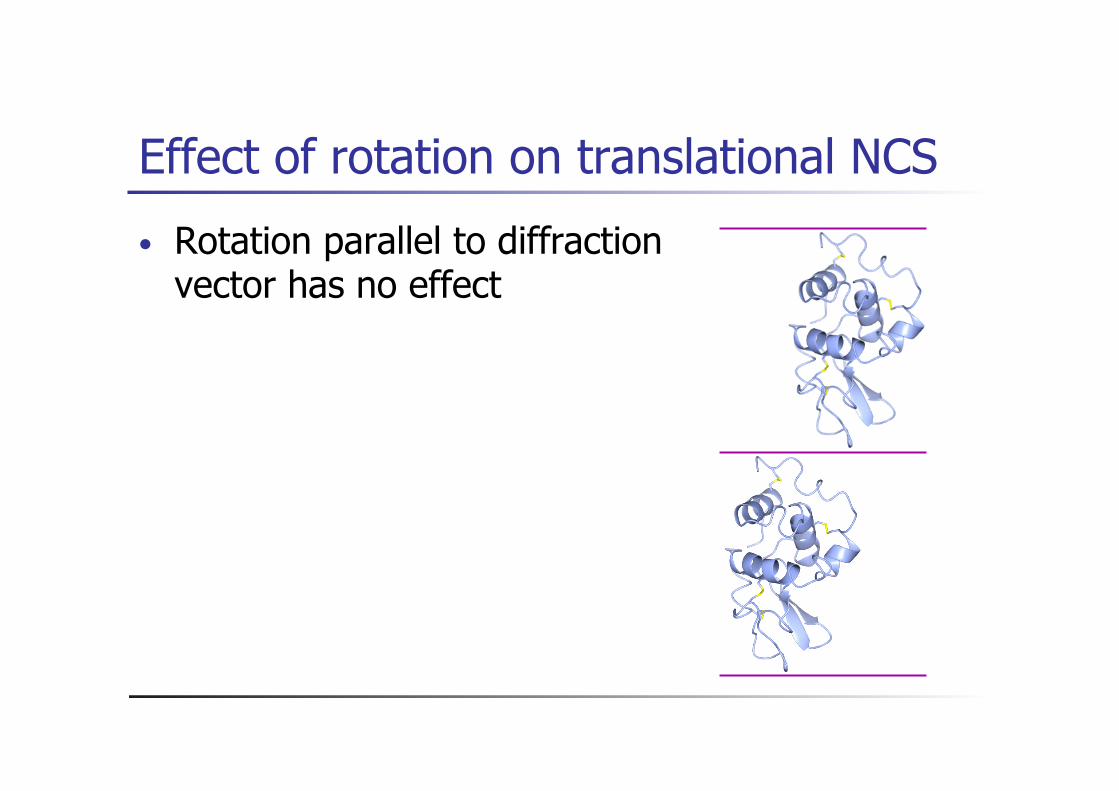
Effect of rotation on translational NCS

•  Rotation parallel to diffraction vector has no effect

Effect of rotation on translational NCS

•  Rotation parallel to diffraction vector has no effect

•  Rotation around other axes reduces correlation

•  Random coordinate differences between copies reduce correlation

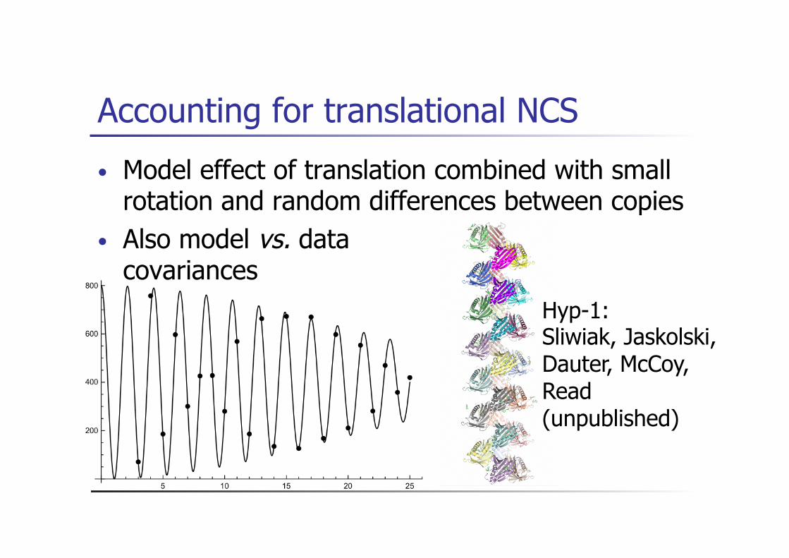
Accounting for translational NCS

•  Model effect of translation combined with small rotation and random differences between copies

•  Also model vs. data covariances

Hyp-1: Sliwiak, Jaskolski, Dauter, McCoy, Read (unpublished)

Other potential applications

•  SIR likelihood target •  SIR phasing •  joint refinement of native and liganded structures

•  Fast translation function for SAD target •  Understanding of solvent flattening

Acknowledgements

•  Phaser: Airlie McCoy, Laurent Storoni, Gábor Bunkóczi, Rob Oeffner

•  Hyp-1: Mariusz Jaskolski, Joanna Sliwiak, Zbyszek Dauter