structure of a flat plate boundary layer subjected to free ...ndjilali/papers/ijcfd_peneau et...

Structure of a Flat Plate Boundary Layer Subjected toFree-Stream Turbulence

FREDERIC PENEAUa,*, HENRI CLAUDE BOISSONb, ALAIN KONDJOYANc and NED DJILALId

aCERAM EAI Tech, 157 rue Albert Einstein, BP 085, 06902 Sophia Antipolis Cedex, France; bIMFT, av Pr Camille Soula, 31400 Toulouse, France;cINRA, S.R.V., 63122 Saint Genes Champanelle, France; dDepartment of Mechanical Engineering, University of Victoria, Victoria, BC, Canada V8W 3P6

The structure near the flat plate leading edge of an incompressible boundary layer subjected to free-stream turbulence is investigated using large eddy simulation (LES) with a dynamic mixed subgrid-scale model. Free-stream turbulent intensities ranging from 1.5 to 10% are investigated. The evolutionsof the velocity, temperature and turbulent intensity profiles inside the boundary layer and thecharacteristic length scales are analyzed and compared to a laminar flat plate boundary layer. Theimpact of the free-stream turbulence is examined for Reynolds numbers ranging from 0 (leading edge ofthe flat plate) to Rex ¼ 80; 000 by using two consecutive spatial LESs. Bypass transition is found tooccur in the early stage of the boundary layer development for all five cases presented here. Theanalysis indicates that the thermal turbulent structures transfer more energy and hence generate morethermal fluctuations in their wake than the dynamic structures.

Keywords: Heat transfer; Free-stream turbulence; Flat plate boundary layer; Large eddy simulations

NOMENCLATURE

Cf Friction coefficient with

free-stream turbulence

Cf 0Friction coefficient without


D ¼ lrCp

Thermal diffusivity

Dt Subgrid diffusivity, turbulent

diffusivity ¼ kv0T 0l=›T=›y

Iu ¼

ffiffiffiffiffiffiffiffiffiffiffiffiffiffiffiffiffiffiffiffiffiffiffiffiffiffiffiffiffiffiffiffiffiffiffiffiu2rmsþv2

rmsþw2rms

qUe

Turbulent intensity

h, he, hw Fluid enthalpy, free-stream

fluid enthalpy and wall

fluid enthalpy

L1 ¼kq2

el3=2

Ue›kq2

el›x

Free-stream turbulence

dissipative

length-scale

P ¼ P þ P00 Large eddy decomposition

for the pressure field�P Resolved pressure field

P00 Subgrid pressure field

Pr ¼ nD

Prandtl number

Prt ¼nt

DtTurbulent Prandtl number

qe¼u2

rms þ v2rms þw2

rms

2Turbulent kinetic energy

Rex ¼Uexn

Reynolds number based

on the distance from

the leading edge ‘x’

Reu ¼Ueun

Reynolds number based on

the local momentum

thickness u

St Stanton number with


St0 Stanton number without


T ¼ Tmean þ T 0 Reynolds decomposition

for the temperature field

Tmean Mean temperature

T0 Temperature fluctuations

kT 0l ¼ 0

T rms ¼ kT 0T 0l0:5 Temperature turbulent level

T ¼ T þ T 00 Large eddy decomposition

for the temperature field

T Resolved temperature field

T00 Subgrid temperature field

Tu ¼ urms

UeTurbulent level

ui ¼ Ui þ u0i Reynolds decomposition

for the velocity field

Ui Mean velocity field; U1 ¼ U

longitudinal direction;

U2 ¼ V lateral direction;

U3 ¼ W span-wise

direction

ISSN 1061-8562 print/ISSN 1029-0257 online q 2004 Taylor & Francis Ltd

DOI: 10.1080/10618560310001634177

*Corresponding author. E-mail: [email protected]

International Journal of Computational Fluid Dynamics, February 2004 Vol. 18 (2), pp. 175–188

u0i Velocity

fluctuations

ku0il ¼ 0

u01 ¼ u0 longitudinal direction;

u02 ¼ v0 lateral direction;

u03 ¼ w0 spanwise direction.

Ue Mean free-stream longitudinal

velocity component

ui ¼ �ui þ u00i Large eddy decomposition

for the velocity field

�ui Resolved velocity field

u00i Subgrid velocity field

urms ¼ ku01u0

1l0:5

Longitudinal turbulent

fluctuations

vrms ¼ ku02u0

2l0:5

Lateral turbulent fluctuations

wrms ¼ ku03u0

3l0:5

Span-wise turbulent

fluctuations

d Dynamic boundary layer

thickness

dT Thermal boundary

layer thickness

d1 ¼

ð1

0

1 2U

Ue

� �dy Displacement thickness

d3 ¼

ð1

0

U

Ue

£ 1 2 UUe

� �2� �

dy

Kinetic energy

thickness

D ¼

ð1

0

U

Ue

he 2 h

he 2 hw

� �dy Enthalpy

thickness

u ¼

ð1

0

U

Ue

1 2U

Ue

� �dy Momentum thickness

l Thermal conductivity

m Dynamic viscosity

n ¼mr

Kinematic viscosity

nt Subgrid viscosity, turbulent

viscosity ¼ ku0v0l=›U=›y

r Fluid density

k l Average operator in the span-

wise direction and in time

INTRODUCTION

The influence of high free-stream turbulence on the

dynamics and heat transfer of boundary layer flows is

relevant to many industrial applications and has been the

subject of experimental and theoretical research for some

time. The first studies were performed in the thirties by Fage

and Falkner (1931) who did not observe any influence on

heat transfer in the presumed laminar region. Due to

discrepancies and contradictions in reported findings, the

field remained wide open until the landmark work of

Bradshaw (1974). In a series of studies with his team,

(Simonich and Bradshaw, 1978; Hancock and Bradshaw,

1983, 1989; Baskaran et al., 1989), Bradshaw and his group

analyzed the influence of free-stream turbulence not only in

terms of the turbulence level Tu but also in terms of the

turbulent length scale Le. It was found that if Le is too small

with respect to the boundary layer length scale, then the free-

stream turbulent structures dissipate before reaching the

surface of the plate with no increase in the dynamic activities

of the flow or in heat transfer. In his report of 1974, Bradshaw

noted the importance of the work of Charnay et al. (1971,

1972, 1976) on the interaction mechanisms between the

free-stream flow and the wake of the boundary layer. A few

years later, Dyban et al. (1977), Dyban and Epick (1985)

published a very interesting and original work on the

influence of free-stream turbulence on the laminar region of

the boundary layer. With the focus of both academic and

industrial research at that time on turbulent flow, Dyban

et al.’s work did not receive the attention it deserved.

An increase of 56% in the friction coefficient was observed

at low Reynolds numbers (,20,000) with a free-stream

turbulence level of 12.5%. These results underscored the

importance of the interaction between the boundary layer

and the free-stream near the leading edge. Meanwhile, a

consensus has emerged from the numerous studies on

turbulent boundary layers. Free-stream turbulence does

increase the dynamic and heat transfer in the turbulent

boundary layer and heat transfer seems to be more sensitive

to free-stream turbulence (Pedisius et al., 1979; Meier and

Kreplin, 1980; Blair, 1983a,b). Although this conclusion is

general, there is considerable variation from study to study

on the magnitude of the heat transfer enhancement. Several

studies in the 80s and 90s attempted to model these

phenomena with varying success (Young et al., 1992;

Maciejewski and Moffat, 1992). A review of the main

experimental work can be found in Kondjoyan et al. (2002).

In this paper we present a numerical analysis of the

influence of free-stream turbulence on the “laminar”

boundary layer. Our results are compared to the experimental

data of Dyban et al. (1977) and Dyban and Epick (1985) and

we propose an interpretation of the observed phenomena.

The paper provides first an overview of the numerical model,

the computational procedure and the physical characteristics

of the problem. We then present the evolution of the

velocity and temperature profiles inside the boundary layer in

the presence of free-stream turbulence. The turbulent

intensity and turbulent energy production profiles are

examined and compared to those for a turbulent boundary

layer with no free-stream turbulence. Finally, a physical

interpretation of the results is proposed based on an analysis

of the Reynolds stresses and turbulent Prandtl number.

NUMERICAL METHOD AND SUBGRID

MODELING

The LES Equations and the Subgrid-scale Model

The LES equations are obtained by introducing the

following decomposition in the Navier–Stokes equations:

ui ¼ �ui þ u00i ð1Þ

F. PENEAU et al.176

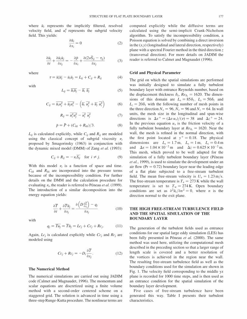
where �ui represents the implicitly filtered, resolved

velocity field, and u00i represents the subgrid velocity

field. This yields:

›�ui

›xi

¼ 0 ð2Þ

›�ui

›tþ

›�ui �uj

›xj

¼ 2›�p

›xi

þ›ð2nSij 2 tijÞ

›xj

ð3Þ

wheret ¼ uiuj 2 �ui �uj ¼ Lij þ Cij þ Rij ð4Þ

withLij ¼ �ui �uj 2 �ui �uj ð5Þ

Cij ¼ �uiu00j þ �uju

00i 2 �ui u00

j þ �uj u00i

� �ð6Þ

Rij ¼ u00i u00

j 2 u00i u00

j ð7Þ

�p ¼ �P þ ðCkk þ RkkÞ=3: ð8Þ

Lij is calculated explicitly, while Cij and Rij are modeled

using the classical concept of subgrid viscosity nt

proposed by Smagorinsky (1963) in conjunction with

the dynamic mixed model (DMM) of Zang et al. (1993):

Cij þ Rij ¼ 2ntSij for i – j: ð9Þ

With this model nt is a function of space and time.

Ckk and Rkk are incorporated into the pressure terms

because of the incompressibility condition. For further

details on the DMM and the calculation procedure for

evaluating nt, the reader is referred to Peneau et al. (1999).

The introduction of a similar decomposition into the

energy equation yields:

›T

›tþ

›T �uj

›xj

¼› D ›T

›xj

� �2 qj

›xj

ð10Þ

with

qj ¼ Tuj ¼ T �uj ¼ Lcj þ Ccj þ Rcj: ð11Þ

Again, Lcj is calculated explicitly while Ccj and Rcj are

modeled using

Ccj þ Rcj ¼ 2Dt

›T

›xj

: ð12Þ

The Numerical Method

The numerical simulations are carried out using JADIM

code (Calmet and Magnaudet, 1996). The momentum and

scalar equations are discretized using a finite volume

method with a second-order centered scheme on a

staggered grid. The solution is advanced in time using a

three-step Runge-Kutta procedure. The nonlinear terms are

computed explicitly while the diffusive terms are

calculated using the semi-implicit Crank-Nicholson

algorithm. To satisfy the incompressibility condition, a

Poisson equation is solved by combining a direct inversion

in the (x,y) (longitudinal and lateral direction, respectively)

plane with a spectral Fourier method in the third direction z

(transversal direction). For more details on JADIM the

reader is referred to Calmet and Magnaudet (1996).

Grid and Physical Parameter

The grid on which the spatial simulations are performed

was initially designed to simulate a fully turbulent

boundary layer with entrance Reynolds number, based on

the displacement thickness d1, Red1¼ 1620: The dimen-

sions of this domain are Lx ¼ 85d1; Ly ¼ 50d1 and

Lz ¼ 20d1 with the following number of mesh points in

the three direction Nx ¼ 96; Ny ¼ 96 and Nz ¼ 64. In wall

units, the mesh size in the longitudinal and span-wise

directions is Dxþ ¼ ðDx·utÞ=ðnÞ ¼ 38 and Dzþ ¼ 24:In the previous equation ut is the friction velocity of a

fully turbulent boundary layer at Red1¼ 1620: Near the

wall, the mesh is refined in the normal direction, with

the first point located at yþ ¼ 0:18: The physical

dimensions are Lx ¼ 1:7 m; Ly ¼ 1 m; Lz ¼ 0:4 m

and Dx ¼ 1:04 £ 1022 m and Dz ¼ 0:625 £ 1022 m.

This mesh, which proved to be well adapted for the

simulation of a fully turbulent boundary layer (Peneau

et al., 1999), is used to simulate the development under an

air flow ðPr ¼ 0:72Þ boundary layer near the leading edge

of a flat plate subjected to a free-stream turbulent

field. The mean free-stream velocity is Ue ¼ 1:23 m=s:The free-stream temperature is Te ¼ 273 K while the wall

temperature is set to Tw ¼ 274 K: Open boundary

conditions are set as ›2 �ui=›n2 ¼ 0; where n is the

direction normal to the exit plane.

THE HIGH FREE-STREAM TURBULENCE FIELD

AND THE SPATIAL SIMULATION OF THE

BOUNDARY LAYER

The generation of the turbulent fields used as entrance

conditions for our spatial large eddy simulation (LES) has

been fully presented in Peneau et al. (2000). The same

method was used here, utilizing the computational mesh

described in the preceding section so that a larger range of

length scale is covered and a better resolution of

the vortices is achieved in the region near the wall.

The resulting free-stream turbulence field as well as the

boundary conditions used for the simulation are shown in

Fig. 1. The velocity field corresponding to the middle yz

plane is recorded for 1000 time steps, and is then used as

an entrance condition for the spatial simulation of the

boundary layer development.

Five cases of free-stream turbulence have been

generated this way. Table I presents their turbulent

characteristics.

STRUCTURE OF FLAT PLATE BOUNDARY LAYER 177

Figures 2 and 3 show the turbulence level and intensity

profiles for the five cases of free-stream turbulent fields

investigated, and Fig. 4 shows the temporal evolution. The

profiles presented were obtained by applying an averaging

operator in the span-wise direction and in time (1000 time

steps). “y ¼ 0 m” corresponds to the position of the flat

plate while “y ¼ 1 m” corresponds to the north boundary

of the domain of calculation. In this direction, the mesh

size increases progressively and hence there is a decrease

in the turbulent levels and intensities as we reach the north

boundary.

This phenomenon is less important for cases D and E

because these turbulent fields were generated with larger

vortices which are better resolved and do not dissipate as

much in this region. The root mean square velocity profiles

for the five cases indicate that the turbulent fields are

almost isotropic and homogeneous except near the north

and south boundaries of the domain, again because of the

boundary conditions imposed there. Note that a constant

free-stream temperature field is imposed such that no rms

temperature profile exists.

The temporal evolution obtained by applying an

averaging operator in the span-wise and lateral direction

on the entrance velocity signals shows an exponential

decay of the turbulence level similar to the spatial decay of

grid-generated turbulence.

In order to extend the Reynolds number of the

simulations, two successive spatial simulations were

FIGURE 4 Temporal evolution of the turbulence levels.

FIGURE 3 Turbulent intensity profiles.

FIGURE 2 Turbulent level profiles.

TABLE I Turbulent characteristics of the five free-stream turbulentfields generated

Tu in % Iu in %

Case A 1 2Case B 3 5Case C* 3 5Case D 5 8Case E 10 16

* The case C was generated with bigger vortices to analyse the influence of theturbulence length-scale on the wall transfer.

FIGURE 1 Lateral component of a typical free-stream vorticity field.(Colour version available to view online.)

F. PENEAU et al.178

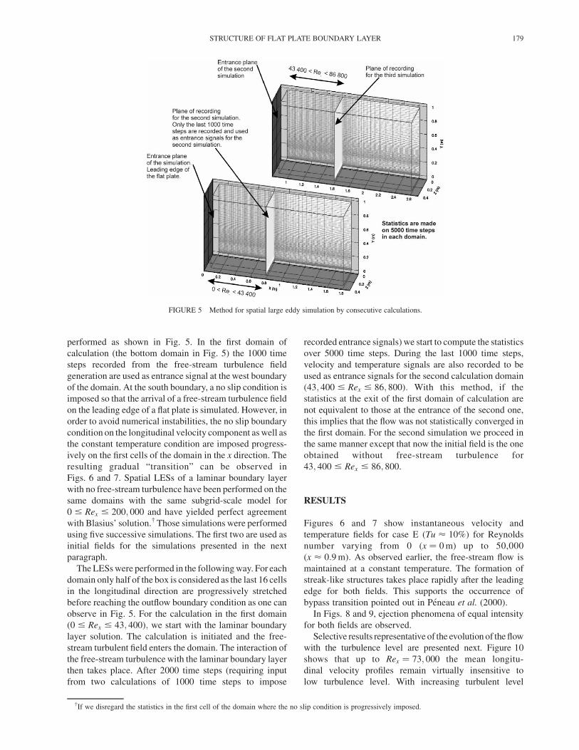
performed as shown in Fig. 5. In the first domain of

calculation (the bottom domain in Fig. 5) the 1000 time

steps recorded from the free-stream turbulence field

generation are used as entrance signal at the west boundary

of the domain. At the south boundary, a no slip condition is

imposed so that the arrival of a free-stream turbulence field

on the leading edge of a flat plate is simulated. However, in

order to avoid numerical instabilities, the no slip boundary

condition on the longitudinal velocity component as well as

the constant temperature condition are imposed progress-

ively on the first cells of the domain in the x direction. The

resulting gradual “transition” can be observed in

Figs. 6 and 7. Spatial LESs of a laminar boundary layer

with no free-stream turbulence have been performed on the

same domains with the same subgrid-scale model for

0 # Rex # 200; 000 and have yielded perfect agreement

with Blasius’ solution.† Those simulations were performed

using five successive simulations. The first two are used as

initial fields for the simulations presented in the next

paragraph.

The LESs were performed in the following way. For each

domain only half of the box is considered as the last 16 cells

in the longitudinal direction are progressively stretched

before reaching the outflow boundary condition as one can

observe in Fig. 5. For the calculation in the first domain

ð0 # Rex # 43; 400Þ; we start with the laminar boundary

layer solution. The calculation is initiated and the free-

stream turbulent field enters the domain. The interaction of

the free-stream turbulence with the laminar boundary layer

then takes place. After 2000 time steps (requiring input

from two calculations of 1000 time steps to impose

recorded entrance signals) we start to compute the statistics

over 5000 time steps. During the last 1000 time steps,

velocity and temperature signals are also recorded to be

used as entrance signals for the second calculation domain

ð43; 400 # Rex # 86; 800Þ: With this method, if the

statistics at the exit of the first domain of calculation are

not equivalent to those at the entrance of the second one,

this implies that the flow was not statistically converged in

the first domain. For the second simulation we proceed in

the same manner except that now the initial field is the one

obtained without free-stream turbulence for

43; 400 # Rex # 86; 800.

RESULTS

Figures 6 and 7 show instantaneous velocity and

temperature fields for case E ðTu < 10%Þ for Reynolds

number varying from 0 ðx ¼ 0 mÞ up to 50,000

ðx < 0:9 mÞ: As observed earlier, the free-stream flow is

maintained at a constant temperature. The formation of

streak-like structures takes place rapidly after the leading

edge for both fields. This supports the occurrence of

bypass transition pointed out in Peneau et al. (2000).

In Figs. 8 and 9, ejection phenomena of equal intensity

for both fields are observed.

Selective results representative of the evolution of the flow

with the turbulence level are presented next. Figure 10

shows that up to Rex ¼ 73; 000 the mean longitu-

dinal velocity profiles remain virtually insensitive to

low turbulence level. With increasing turbulent level

†If we disregard the statistics in the first cell of the domain where the no slip condition is progressively imposed.

FIGURE 5 Method for spatial large eddy simulation by consecutive calculations.


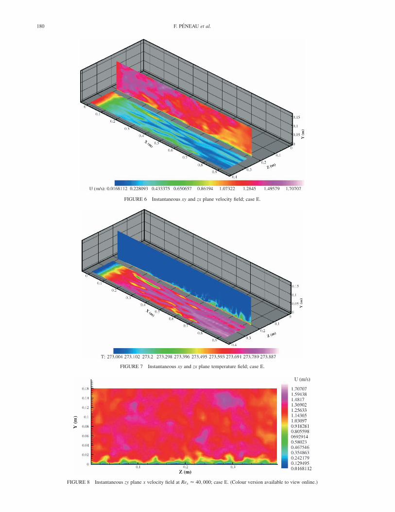
FIGURE 6 Instantaneous xy and zx plane velocity field; case E.

FIGURE 7 Instantaneous xy and zx plane temperature field; case E.

FIGURE 8 Instantaneous zy plane x velocity field at Rex < 40; 000; case E. (Colour version available to view online.)

F. PENEAU et al.180

(shown in Fig. 11), a progressive flattening of the velocity

profile takes place inducing the formation of a wake.

The wake formation was also observed experimentally

by Dyban et al. (1977) and Dyban and Epick (1985) shown

in Fig. 12.

Figure 13 shows a more pronounced flattening of the

temperature profile compared to the velocity profile. This

was reported in Peneau et al. (2000) and is confirmed here

with the finer grid simulations presented for both lower

turbulent levels and higher Reynolds numbers. At higher

turbulence levels we can observe in Fig. 14 that for case E,

the profile is closer to a turbulent profile even though no

logarithmic region is yet apparent.

The spatial evolution of the boundary layer thicknesses

is plotted in Figs. 15 and 16. The absence of dis-

continuities around Rex < 40; 000 proves, at least up to

Rex ¼ 80; 000; that the consecutive simulations method-

ology used does not perturb the spatial evolution. It also

shows that at a moderate turbulent level, there is no

significant thickening of the boundary layer in contrast

with higher turbulence levels. The thickening explains the

flattening of the velocity profile and, consequently, the

reduction of the displacement thickness and increase of

momentum thickness. The corresponding phenomena for

the thermal field are even more important, hence the

higher flattening of the temperature profile (Fig. 17) when

the boundary layer thickness is used for normalizing the

data.

The higher thickening of the thermal boundary layer is

explained by the value of the turbulent Prandtl number

inside the boundary layer. As shown in Figs. 18 and 19,

whereas Prt is close to 1 at low turbulence levels, Prt , 1

over most of the boundary layer at a higher turbulence

level, such as in case E. This implies the thermal

turbulent structures transfer more energy and hence

generate higher fluctuations in their wake than the

dynamic structures.

Although at low turbulence levels no thickening of the

boundary layer and no flattening of the velocity profile is

observed, there are nevertheless some important phenom-

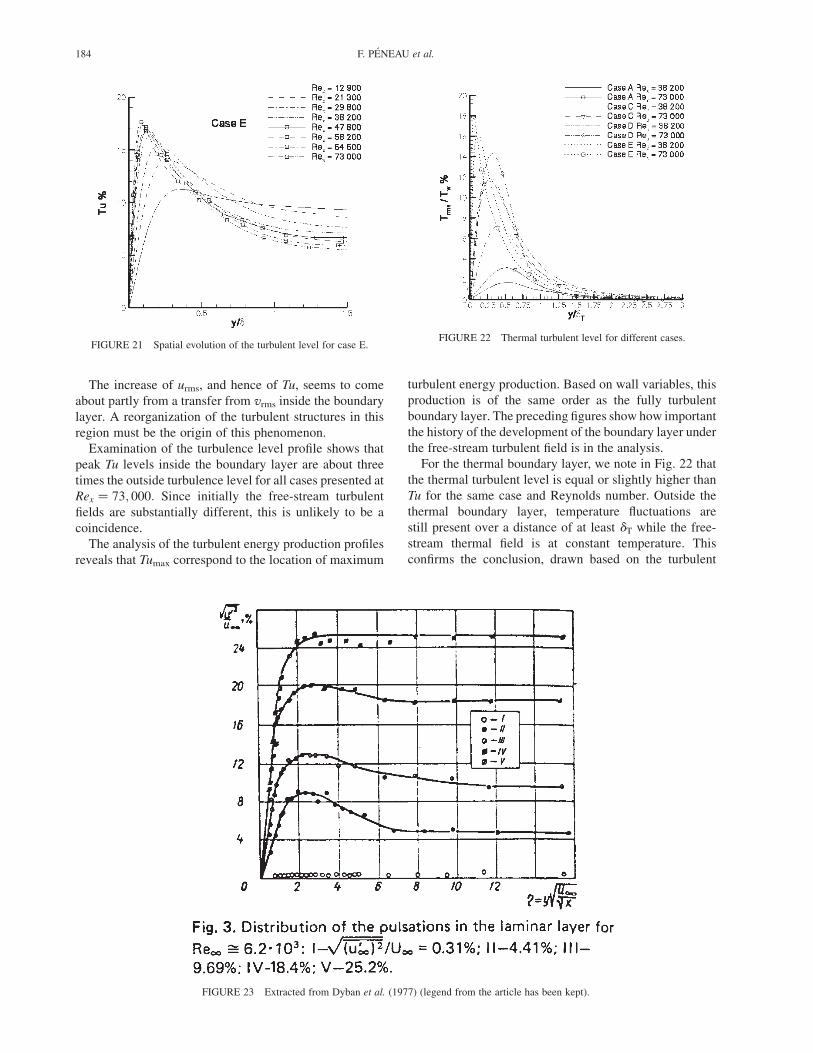
ena that occur inside the boundary layer. Figures 20–22

show that a rapid increase of the maximum turbulence

level takes place inside the boundary layer, and values

exceeding free-stream levels are attained. This points to a

mechanism of turbulent energy production inside the

boundary layer. These observations are consistent with

the experimental measurements of Dyban et al. (1977)

(see Fig. 23).

FIGURE 9 Instantaneous zy plane temperature field at Rex < 40; 000; case E. (Colour version available to view online.)

FIGURE 10 U velocity profile spatial evolution for case A. FIGURE 11 U velocity profile spatial evolution for case D.


FIGURE 12 Extracted from Dyban et al. (1977) (legend from the article has been kept).

FIGURE 13 Temperature profile spatial evolution for case D. FIGURE 14 U velocity profile spatial evolution for case E.

F. PENEAU et al.182

FIGURE 15 Spatial evolution of the boundary layer thicknesses (in m)for case B.

FIGURE 16 Spatial evolution of the boundary layer thicknesses (in m)for case E.

FIGURE 17 Spatial evolution of the thermal boundary layerthicknesses (in m) for case E.

FIGURE 18 Spatial evolution of the turbulent Prandtl number for case A.

FIGURE 19 Spatial evolution of the turbulent Prandtl number for case E.

FIGURE 20 Spatial evolution of the turbulent level for case A.


The increase of urms, and hence of Tu, seems to come

about partly from a transfer from vrms inside the boundary

layer. A reorganization of the turbulent structures in this

region must be the origin of this phenomenon.

Examination of the turbulence level profile shows that

peak Tu levels inside the boundary layer are about three

times the outside turbulence level for all cases presented at

Rex ¼ 73; 000: Since initially the free-stream turbulent

fields are substantially different, this is unlikely to be a

coincidence.

The analysis of the turbulent energy production profiles

reveals that Tumax correspond to the location of maximum

turbulent energy production. Based on wall variables, this

production is of the same order as the fully turbulent

boundary layer. The preceding figures show how important

the history of the development of the boundary layer under

the free-stream turbulent field is in the analysis.

For the thermal boundary layer, we note in Fig. 22 that

the thermal turbulent level is equal or slightly higher than

Tu for the same case and Reynolds number. Outside the

thermal boundary layer, temperature fluctuations are

still present over a distance of at least dT while the free-

stream thermal field is at constant temperature. This

confirms the conclusion, drawn based on the turbulent

FIGURE 21 Spatial evolution of the turbulent level for case E.FIGURE 22 Thermal turbulent level for different cases.

FIGURE 23 Extracted from Dyban et al. (1977) (legend from the article has been kept).

F. PENEAU et al.184

Prandtl number, that the thermal boundary layer transfers

more energy.

The analysis of the correlations kT 0T 0l; ku0T 0l and kv0T 0linside the boundary layer reveals that the temperature

fluctuations are aligned with v0. However, although up to

the peak of Tumax the amplitude of Trms is directly

correlated to urms, after that point the correlation weakens

until, in the wake of the boundary layer ku0T 0l , kT 0T 0l ,kv0T 0l (see Figs. 24 and 25).

We deduce that the thermal fluctuations are

convected by the v velocity field and this explains

why the temperature fluctuations do not vanish outside

the boundary layer. From this analysis we can conclude

that the v velocity field feeds the thermal boundary

layer in turbulent energy through the wake. kw0T 0l is

negligible throughout the computational domain.

Figures 26 – 29 show the impact of the above

phenomena on wall shear stress and heat transfer

coefficients, both of which are above the laminar

values for Rex . 20; 000: This increase is linked to

the amplitude of the free-stream turbulence level.

For the case E, Cf and St reach the turbulent value at

Rex < 70; 000 or Reu < 200: For this case we

note that wall coefficients do not change much for Rex .

20; 000; and as a first step to correlate wall transfer and

free-stream turbulence a fit of the formffiffiffiffiffiffiffiRex

pis proposed

for Cf/Cf lam and St/Stlam in Figs. 30 and 31.

Cases B and C in these figures exhibit the same increase

of wall transfer and with no influence of the dissipative

length scale. Furthermore, the temperature field is no more

sensitive to free-stream turbulence than the velocity field

since the same expressions fit the data. This appears to be

in contradiction with the numerical and experimental

observations. The answer to this contradiction lies in the

rapid thickening of the boundary layers observed

previously. Indeed, if instead of expressing the laminar

value of Cf and St in terms of Rex, we express them in

FIGURE 24 Spatial evolution of the velocity temperature correlationfor case E. —: Rex ¼ 16; 800; –-– –: Rex ¼ 33; 700; · · ·: Rex ¼ 55; 000;–-– –: Rex ¼ 71; 900:

FIGURE 25 Spatial evolution of the velocity temperaturecorrelation for case E. The same sign convention as in Fig. 24 is used—: Rex ¼ 16; 800; –-– –: Rex ¼ 33; 700; · · ·: Rex ¼ 55; 000; –-– –:Rex ¼ 71; 900:

FIGURE 26 Influence of the free-stream turbulence on the frictioncoefficient.

FIGURE 27 Influence of the free-stream turbulence on the frictioncoefficient based on the momentum thickness.


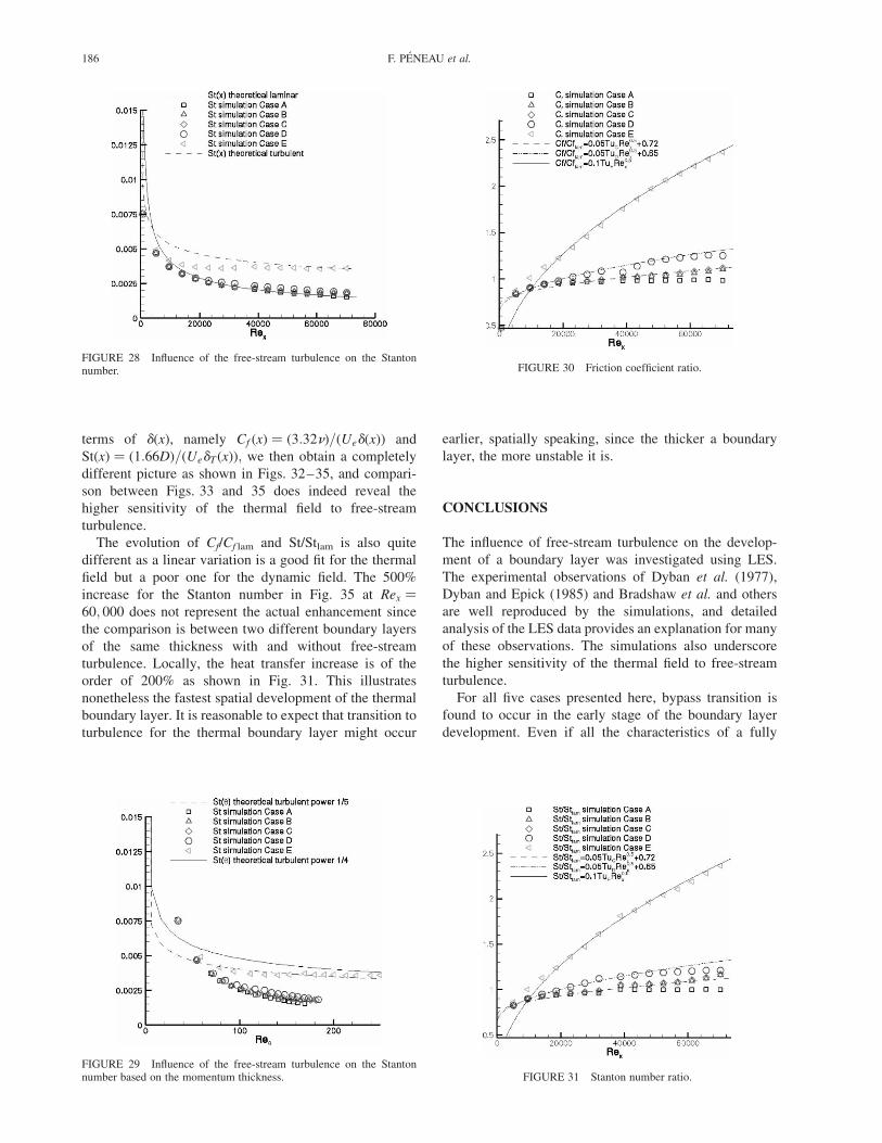
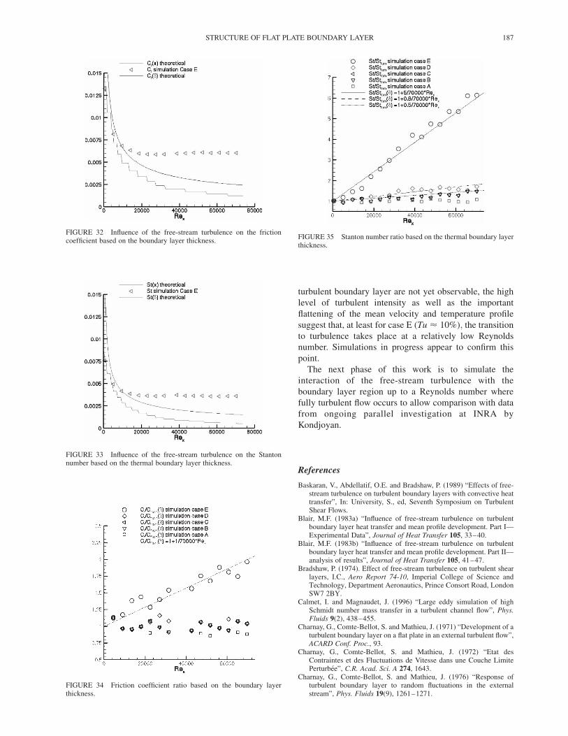
terms of d(x), namely Cf ðxÞ ¼ ð3:32nÞ=ðUedðxÞÞ and

StðxÞ ¼ ð1:66DÞ=ðUedT ðxÞÞ; we then obtain a completely

different picture as shown in Figs. 32–35, and compari-

son between Figs. 33 and 35 does indeed reveal the

higher sensitivity of the thermal field to free-stream

turbulence.

The evolution of Cf/Cf lam and St/Stlam is also quite

different as a linear variation is a good fit for the thermal

field but a poor one for the dynamic field. The 500%

increase for the Stanton number in Fig. 35 at Rex ¼

60; 000 does not represent the actual enhancement since

the comparison is between two different boundary layers

of the same thickness with and without free-stream

turbulence. Locally, the heat transfer increase is of the

order of 200% as shown in Fig. 31. This illustrates

nonetheless the fastest spatial development of the thermal

boundary layer. It is reasonable to expect that transition to

turbulence for the thermal boundary layer might occur

earlier, spatially speaking, since the thicker a boundary

layer, the more unstable it is.

CONCLUSIONS

The influence of free-stream turbulence on the develop-

ment of a boundary layer was investigated using LES.

The experimental observations of Dyban et al. (1977),

Dyban and Epick (1985) and Bradshaw et al. and others

are well reproduced by the simulations, and detailed

analysis of the LES data provides an explanation for many

of these observations. The simulations also underscore

the higher sensitivity of the thermal field to free-stream

turbulence.

For all five cases presented here, bypass transition is

found to occur in the early stage of the boundary layer

development. Even if all the characteristics of a fully

FIGURE 28 Influence of the free-stream turbulence on the Stantonnumber.

FIGURE 29 Influence of the free-stream turbulence on the Stantonnumber based on the momentum thickness.

FIGURE 30 Friction coefficient ratio.

FIGURE 31 Stanton number ratio.

F. PENEAU et al.186

turbulent boundary layer are not yet observable, the high

level of turbulent intensity as well as the important

flattening of the mean velocity and temperature profile

suggest that, at least for case E ðTu < 10%Þ; the transition

to turbulence takes place at a relatively low Reynolds

number. Simulations in progress appear to confirm this

point.

The next phase of this work is to simulate the

interaction of the free-stream turbulence with the

boundary layer region up to a Reynolds number where

fully turbulent flow occurs to allow comparison with data

from ongoing parallel investigation at INRA by

Kondjoyan.

References

Baskaran, V., Abdellatif, O.E. and Bradshaw, P. (1989) “Effects of free-stream turbulence on turbulent boundary layers with convective heattransfer”, In: University, S., ed, Seventh Symposium on TurbulentShear Flows.

Blair, M.F. (1983a) “Influence of free-stream turbulence on turbulentboundary layer heat transfer and mean profile development. Part I—Experimental Data”, Journal of Heat Transfer 105, 33–40.

Blair, M.F. (1983b) “Influence of free-stream turbulence on turbulentboundary layer heat transfer and mean profile development. Part II—analysis of results”, Journal of Heat Transfer 105, 41–47.

Bradshaw, P. (1974). Effect of free-stream turbulence on turbulent shearlayers, I.C., Aero Report 74-10, Imperial College of Science andTechnology, Department Aeronautics, Prince Consort Road, LondonSW7 2BY.

Calmet, I. and Magnaudet, J. (1996) “Large eddy simulation of highSchmidt number mass transfer in a turbulent channel flow”, Phys.Fluids 9(2), 438–455.

Charnay, G., Comte-Bellot, S. and Mathieu, J. (1971) “Development of aturbulent boundary layer on a flat plate in an external turbulent flow”,ACARD Conf. Proc., 93.

Charnay, G., Comte-Bellot, S. and Mathieu, J. (1972) “Etat desContraintes et des Fluctuations de Vitesse dans une Couche LimitePerturbee”, C.R. Acad. Sci. A 274, 1643.

Charnay, G., Comte-Bellot, S. and Mathieu, J. (1976) “Response ofturbulent boundary layer to random fluctuations in the externalstream”, Phys. Fluids 19(9), 1261–1271.

FIGURE 32 Influence of the free-stream turbulence on the frictioncoefficient based on the boundary layer thickness.

FIGURE 33 Influence of the free-stream turbulence on the Stantonnumber based on the thermal boundary layer thickness.

FIGURE 34 Friction coefficient ratio based on the boundary layerthickness.

FIGURE 35 Stanton number ratio based on the thermal boundary layerthickness.


Dyban, E.P. and Epick, E.Y (1985). Transferts de Chaleur etHydrodynamique dans les Ecoulements Rendus Turbulents.Monograph translated from Russian at I.N.R.A., available from A.Kondjoyan.

Dyban, E.P., Epick, E.Y. and Surpun, T.T. (1977) “Characteristics of thelaminar layer with increased turbulence of the outer stream”, Int.Chem. Eng. 17(3), 501–504.

Fage, A. and Falkner, V.M. (1931) “On the relationship between heattransfer and surface friction for laminar flow”, Br. Aero. Res. CouncilR and M, 1408.

Hancock, P.E. and Bradshaw, P. (1983) “The effect of free-stream turbulence on turbulent boundary layers”, J. Fluids. Eng. 105,284–289.

Hancock, P.E. and Bradshaw, P. (1989) “Turbulence structure of aboundary layer beneath a turbulent free-stream”, J. Fluid. Mech. 205,45–76.

Kondjoyan, A., Peneau, F. and Boisson, H.C. (2002) “Effect of highfree-stream turbulence on heat transfer between plates and airflows: a review of existing experimental results”, Int. J. Therm. Sci.41, 1–16.

Maciejewski, P.K. and Moffat, R.J. (1992) “Heat transfer with very highfree-stream turbulence: part II analysis of the results”, ASME J. HeatTransfer 114, 834–839.

Meier, H.U. and Kreplin, H.P. (1980) “Influence of free-streamturbulence on boundary-layer development”, AIAA 18(1), 11–15.

Pedisius, A.A., Kazimekas, P.V. and Slanciauskas, A.A. (1979) “Heattransfer from a plate to a high-turbulence airflow”, Heat TransferSoviet Res. 11(5), 125–134.

Peneau, F., Legendre, D., Magnaudet, J. and Boisson, H.C. (1999) “Largeeddy simulation of a spatially growing boundary layer using adynamic mixed subgrid-scale model”, Symposium ERCOFTAC onDirect and Large Eddy Simulation, (Cambridge).

Peneau, F., Boisson, H.C. and Djilali, N. (2000) “Large eddy simu-lation of the influence of high free-stream turbulence on a spatiallyevolving boundary layer”, Int. J. Heat and Fluid Flow 21, 640–647.

Simonich, J.C. and Bradshaw, P. (1978) “Effect of free-stream turbulenceon heat transfer through a turbulent boundary layer”, Trans. ASME J.of Heat Transfer 100, 671–677.

Smagorinsky, J. (1963) “General circulation experiments with theprimitive equations”, Mon. Weather Rev. 93, 99.

Young, C.D., Han, Y., Huang, Y. and Rivir, R.B. (1992) “Influence of jetgrid turbulence on flat plate turbulent boundary layer and heattransfer”, J. Heat Transfer 114, 64–72.

Zang, Y., Street, R.L. and Koseff, J.R. (1993) “A dynamic mixed subgrid-scale model and its application to turbulent recirculating flows”,Phys. Fluids A5(12), 3186–3196.

F. PENEAU et al.188

structure of a flat plate boundary layer subjected to free ...ndjilali/papers/ijcfd_peneau et...

Documents