structure of murnomomiimmu - defense …. monitoring agency name a aodress(ol difioert imm c...
TRANSCRIPT
AD-A130 468 INFRARED RADIANCE STRUCTURE OF THE AURORA AND AIRGLOW I/(U) PHOTOMETRICS INC WOBURN MA I L KOFSKY ET AL.30 JUN 82 PHM-TR-82-02 AFGL-TR-82-0220 F19628-80-C-0134
UNCLASSIFIED F/G 4/1 NLmurnomomiimmuEhhEEmhhhohmhEEEEmhEmhhhEE-EEEhEE
Ehmhhhmhhhu
EIEIIIIIEIIIII-El..III
11111~ * ~ 128 511111L 12
L3
11111 o
1.1 ,1.8
111- 1111
MICROCOPY RESOLUTION TEST CHARTNATIONAL BUREAU OF STANDARDS-193 A

IAFGL-TR-82-0220
(00INFRARED RADIANCE STRUCTURE OF THE AURORA AND AIRGLOW
I.L. Ksk
L.McVay
C:::1 PhotoMetrics, Inc.4 Arrow DriveWoburn, MA 01801
30 June 1982
scientific Report No. 2
Approved for public release; distribution unlimited
*Prepared for DTIC__ AIR FORCE GEOPHYSICS LABORATORY JUL 8198
a - AIR FORCE SYSTEMS CON MAND JL18ILLJ UNITED STATES AIR FORCE'
M... . HANSCOM AFB, MASSACHUSETTS 01731
B3 O 18
UnclassifiedeCUFmTY CLASSIPICATIOwI OF TIS PAGEr & Don. asemu_ _ _
REPORT DOCUMENTATION PAGE _ _ _AD _____T____ _i__SBEPOlt COMPLTOro'w1. 04PONT NUMBER 0 VT Acceftwo "a. AUIPIEIT* s CArTALOG MIWealk
AFGL-TR-82-0220 r1Ay D -A_ 5_ /66L TITLE (a neI.) - S. TYPE OF NIPONT a PEIOD COVERED
INFRARED RADIANCE STRUCTURE OF Scientific-,THE AURORA AND AIRGLOW 1%,N. 2
em.. mO- EPA' m7. AUTNO( S.. ACT ON GN&NT NUMSCla.)
I.L. Kofsky L. McVay F19628-80-C-0134J.L. Barrett
S. PENONMING OROANIZATION NAME AND ADDRESS '0. PRIOGRAMLEMIT. PROJECT. TASK
PhotoMetrics, Inc. 62101F
Arrow Drive 767011AFoburn. Massachusetts 01801
It. CONTROLLING OFFICE NAME AND ADDRESS 12. REPORT DATE
Air Force Geophysics Laboratory 30 June 82Hanscom AFB, Massachusetts 01731 , U1NFo PAoESMonitor/Robert E. Pierce/OPR 168
14. MONITORING AGENCY NAME a AODRESS(ol dIfIoert Imm C nef..ilne O1ro) IS. SECURITY CLASS. (oh #l IAMJ
Unclassified
T "- DECLASS PIC ATION/OOUNGNADNGSCHEDULE
1I. DISTRI§UTIO* STATEMENT $ 1. Sl. Rflpr#)
Approved for public release; distribution unlimited
I. DISTRInUTION STATEMENT (of tA. C40au1ecf .Imr I- 9I.eh 20. If dXlafe" h.o Rifo.p.
16 SUPPLEMENTARY NOTES
It K EY WORDS fCmofin., O toveto $$do it n .e ola md 1d*.liv II, lork .,, bw)
AuroraAuroral Occurrence AirgaowAuroral Irregularities -Infrared BaurllnceAirgiow Irregularities d Surveillance
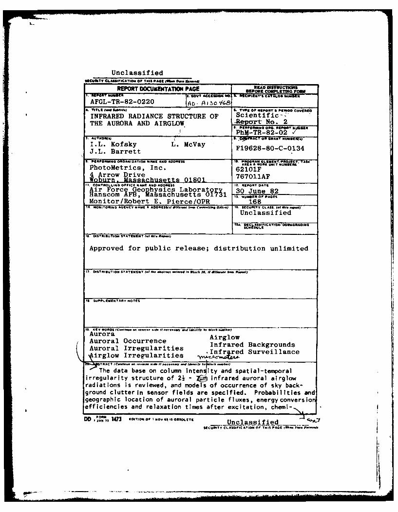
irregularity structure of 21 infrared auroral airglow [radiations is reviewed, and models of occurrence of sky back- I
ground clutter in sensor fields are specified. Probabilities andgeographic location of auroral particle fluxes, energy conversionefficiencies and relaxation times after excitation, chemi-
DO , s 1473 EO*TONOP NOV51 ,SOL-ETE UnclassifiedSICURITY CLASSIFICAYION O THIS PAGE RY.. Ir;a PN-mIl
Unclassified +,Jzc .k, Z-IScuftUTV CL.*SUaFICATICOi OF 141S VA*6(fNW D0. Eal~
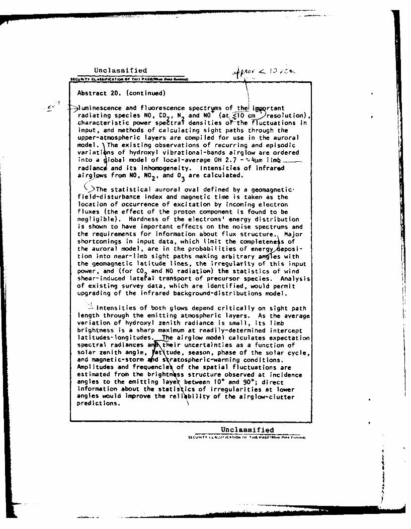
Abstract 20. (continued)
-luminescence and fluorescence spectryms of the imlrtant
radiating species NO, CO , N and NO (at Oh cmjresoution)characteristic power spe~traT densities of-the fluctuations ininput, and methods of calculating sight paths through theupper-atmospheric layers are compiled for use in the auroralmodel. The existing observations of recurring and episodicvariations of hydroxyl vibrational-bands airglow are orderedinto a lobal model of local-average OH 2.7 -% 4lim limb
radiancd and its inhomogeneity. Intensities of infraredairgiows from NO, NO2, and 03 are calculated.
/)The statistical auroral oval defined by a geomagnetic"field-disturbance index and magnetic time is taken as thelocation of occurrence of excitation by incoming electronfluxes (the effect of the proton component is found to benegligible). Hardness of the electrons' energy distributionis shown to have important effects on the noise spectrums andthe requirements for information about flux structure. Majorshortcomings in input data, which limit the completene s ofthe auroral model, are in the probabilities of energy eposi-tion into near-limb sight paths making arbitrary ae es withthe geomagnetic latitude lines, the irregularity of this inputpower, and (for CO and NO radiation) the statistics of windshear-induced latefal transport of precursor species. Analysisof existing survey data, which are identified, would permitupgrading of the infrared background-distributions model.
-- Intensities of both glows depend critically on sight pathlength through the emitting atmospheric layers. As the averagevariation of hydroxyl zenith radiance is small, its limbbrightness is a sharp maximum at readily-determined interceptlatitudes-longitudes. The airglow model calculates expectationspectral radiances a their uncertainties as a function ofsolar zenith angle, aat~tude, season, phase of the solar cycle,and magnetic-storm d s ratospheric-warming conditions.Amplitudes and frequencie of the spatial fluctuations areestimated from the brightn ss structure observed at incidenceangles to the emitting laye between 10* and 90*; directInformation about the statis ics of irregularities at lowerangles would improve the reli bility of the airglow-clutterpredictions. \
Unclassified%LA.1.11 11 v r)I T"09 PAGF(W ism*. t
M& ,4

FOREWORD
This report reviews the existing data on the occurrence
of short-wavelength infrared sky background clutter due to
aurora and airglow, and specifies models for calculating
occurrence-probability distributions. Section 1 relates these
non-equilibrim emissions to the thermal radiation from the
lower atmosphere. Section 2 discusses the geographic location
location and frequency of excitation of air by auroral particles
and the ensuing reaction processes that result in infrared radia-
ations, and develops a background-noise occurrence model of scope
commensurate with the available input data (Fig 23). In Section
3 the observations of airglow from hydroxyl molecules are ordered
into a global model of mean limb radiance and its fluctuation
structure (Fig 25). Information on 2-1/2 - 7um glows from
the other infrared-active atmospheric species NO, NO2 and 03is presented in two appendixes.
We have attempted to include enough basic information on
luminescence processes in the upper atmosphere to make the re-
port directly useful to designers of measurement systems. The
terminology of auroral radiation and morphology is explained;
a procedure for converting between the coordinate systems of
auroral occurrence and an optical measurement system is given;
example spectral radiance distributions are shown, in engineering
units; and references clarifying (and Justifying) all critical
ideas are presented. The report is written at the technical
standard of the geophysics and aerochemistry communities, toward
stimulating thought on how best to improve the input data that
determine reliability and resolution of the models of infrared
cl utter.
3

The authors express their thanks to the many indivi-
duals who supplied information beyond that available in the
literature, and especially to J. Whalen, E. Weber, A. McIntyre,
R. Huffman, R. Nadile, R. O'Neil, R. Murphy, S. Dandekar, F.
Kneizys (all of Air Force Geophysics Laboratory) and D. Archer,
J. Stephens, T. Degges, R. Eather, F. Kaufman, and G. Caledonia.
The figures were prepared by D.P. Villanucci of PhotoMetrics,
and F. Richards and M. Craig assisted with preparation of the
report. Particular thanks is due Mrs. Carmela C. Rice, who
was responsible for typing the manuscript. Most of the basic
ideas on auroral-infrared occurrence were developed by Lance
McVay, and on hydroxyl airglow by John Barrett. The authors
gratefully acknowledge the support and encouragement of
Dr. Randall E. Murphy of AFGL/OPR.
Accession For
NTIS GRA&1DTIC TABUnannounced CJustifioation
Dy.
Distribution/Availability Codes
Avail and/orIst Special
4_

TABLE OF CONTENTS
SECTION PAGE
Foreword .................................................. 3
1. Introduction ....... *.. . . .. ..... *.*.... ....... ..... 91.1. Context of Auroral-Airgiow Clutter Background ..... 101.2. Scope of This Report ............................. 121.3. Overview of Infrared Aurora and Airgiow ........ 16
1.3.1. Emission Spectrum *..... . .*to.. ...... 0 ... 191o.4. Comparison of Typical Aurora-Airglow and Thermal
Radiance Backgrounds .... *........... .. ... ... . o ... .. o. 201.4.1.* Nadir Radiances ......... ................ o21
1.4.2. Limb Radiance Considerations .................. 251.4.2.1. Limb Enhancements ... o........o........ 27i1.4.2.2. Effects of Limb Enhancements
on Backgrounds Distributions oo...... o 33
2. Auroral Infrared Backgrounds .......... ooo.. ....... o... 342.1. Data Base on Auroral Occurrence and Aerochemistry . ... 34
2 2.2l ccurrenc heOvenlog ............... *.......... 35
2.2.2. Zenith-Flux Occurrence Probabilities ... ... o... 392.2.3. Line-of-Sight Input Occurrence .... too.....o 402.2.4. Inhomogeneity Occurrence ........... o...... too. 41
2.2.4.1. Spatial Inhomogeneity to .............. 412.2.4.2. Temporal Inhomogeneity .. ............. 41
2.2o5. Temporal Correlation of Input Flux ....... 422.3. Contribution of Protons ... ............... o....... o ... 442.4. Altitude Profiles ... ... to... o ................. o..... 45
2.4.1. Particle Energy Distribution 000009*0000000000. 452.4.2. Optical Diagnostics of the Energy Spectrum .... 462.4o3. Dependence of F on a ............. 0... *.......492.4.4o Minimum Energy Flux and Energy Parameter ...... 53
2.5. Auroral Emissions: Fluorescence ... o..... to.... o ...... 542.5.1. "Prompt" Emission Near 4.3jmn .................. 57
2.6o Auroral Emissions; Chemiluminescence andVibraluminescence .. . .. ........... .. 582.6.1. Nitric Oxide .o.............................. 59
2.6.1.*1 * Time Dependence . . .. . . . .. 63I2.6.1.2. Space Dependence .... 0.......... 662.6.1.3. Spatial-Temoral Radiance Variations .. 692.6.1.4. Altitude Profiles . ... 0040064606696. 732.6.1.5. Non-tauror]. NO Fundamental Band
2.6.2. Carbon Dioxide . .. ... 000 ... . . ....... *0000 742.6.2.1. Excitation Transfer and Residence
*Times of Vibrational Energy .... o... o. 752.6.2.2. Impact on Background of the Conver-
sion Efficiency and Residence Time ... 81
2.6.2.3. Other 4.3m Emission(s) ..... o..o .... 82
t 5

TABLE OF CONTENTS (concluded)SECTION PAGE
2.7. Specification of Spatial and Temporal Input Struc-ture ................................................ 86
2.d. An Occurrence Model .............................. .. 892.8.1. Auroral Activity Index ....................... 902.8.2. Dimensions and Location of the Occurrence
Region ....................................... 912.8.2.1. Conversion to Geographic Coordin-
ates and Universal Time ............. 942.8.3. Occurrence Within the Oval ................... 98
2.8.3.1. DMSP Images ........................ 992.8.3.2. Other Data .......................... 1012.8.3.3. Zenith Occurrence ................... 1032.8.3.4. Slant-Path Input .................... 1042.8.3.5. Temporal and Spatial Structure ...... 104
2.8.4. A First-Generation Auroral Clutter Model ..... 1052.9. Discussion ........... *.................0.........0..... 109
3. Airglow Infrared Background ...... 111
3.2. Radiance Variability ........ . ... ...... ... 1173.2.1. Diurnal Variations .... ....... o............ 1193.2.2. Seasonal Variations ........... .......... o 1203.2.3. Solar Cycle Variations ..... ..... 1213.2.4. Magnetic Storm-Induced Variations ... o....... 1223.2.5. Stratospheric Warming-Induced Enhancement .... 1233.2.6. Latitude Effects ........ ........ . 1243.2.7. Diurnal Model . .. ... ... .. . ........ o...oo.. . 124
3.3. Emission Spectrum ...... ..... ........ .. ... * ...... 1263.4. Calculations of Column Intensity ... ...... o ....... 1293.5. Clutter Statistics ............... .... o..... 132
3.5.1. Zenith Data ................ ........... 1333.5.2. Low Elevation-Angle Data ..... o* ...... 1353.5.3. Clutter Amplitude and Frequency ......... 136
3.6. Hydroxyl Data Base ...... .......................... 139
References .. 00.... ... .. ...... .. . 0..... 140
Appendix I Nitric Oxide Vibrational-Overtone Airglow ...... 149Appendix II Infrared Airglows from 03 and NO 2 ......... o--. 154Appendix III Auroral Input-Intensity gistribution Data
from Dynamics Explorer ....................... 163
6
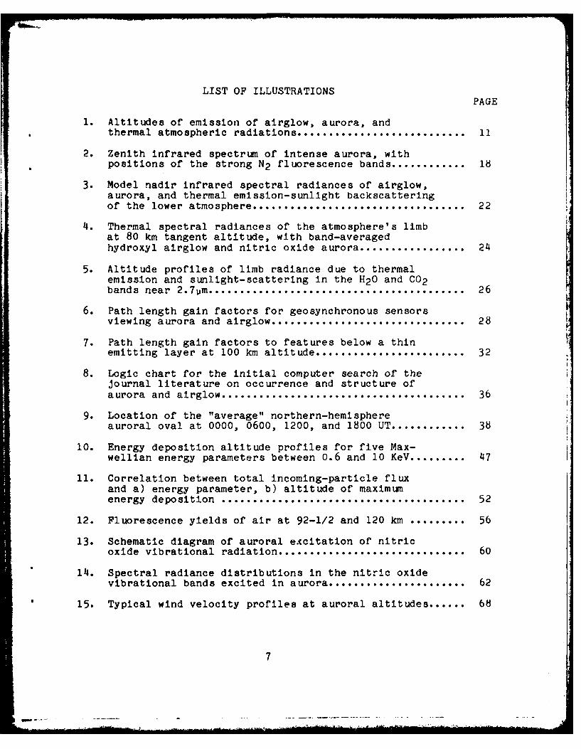
LIST OF ILLUSTRATIONSPAGE
1. Altitudes of emission of airglow, aurora, andthermal atmospheric radiations ........................... 11
2. Zenith infrared spectrum of intense aurora, withpositions of the strong N 2 fluorescence bands ............ 18
3. Model nadir infrared spectral radiances of airglow,aurora, and thermal emission-sunlight backscatteringof the lower atmosphere .................................. 22
4. Thermal spectral radiances of the atmosphere's limbat 80 km tangent altitude, with band-averagedhydroxyl airglow and nitric oxide aurora ................. 24
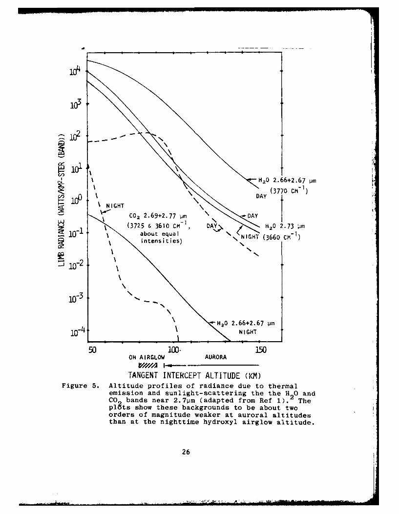
5. Altitude profiles of limb radiance due to thermalemission and sunlight-scattering in the H20 and CO 2bands near 2.7im ......... .... .......................... 26
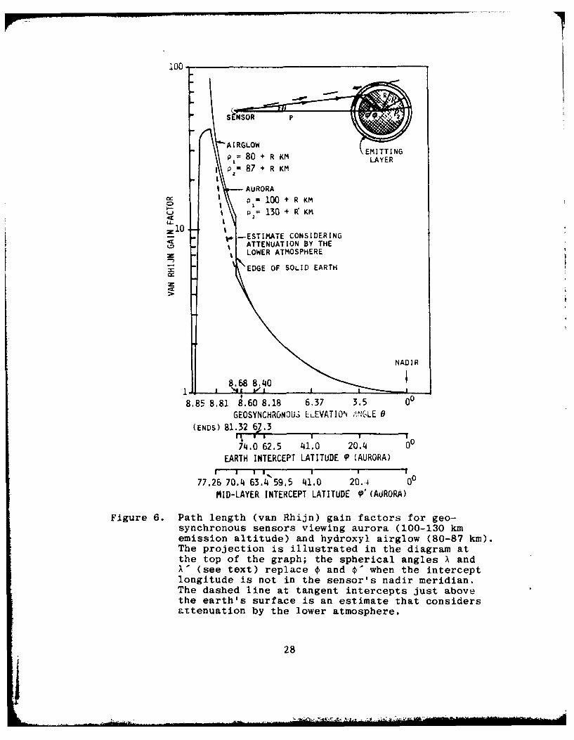
6. Path length gain factors for geosynchronous sensorsviewing aurora and airglow ............................... 28
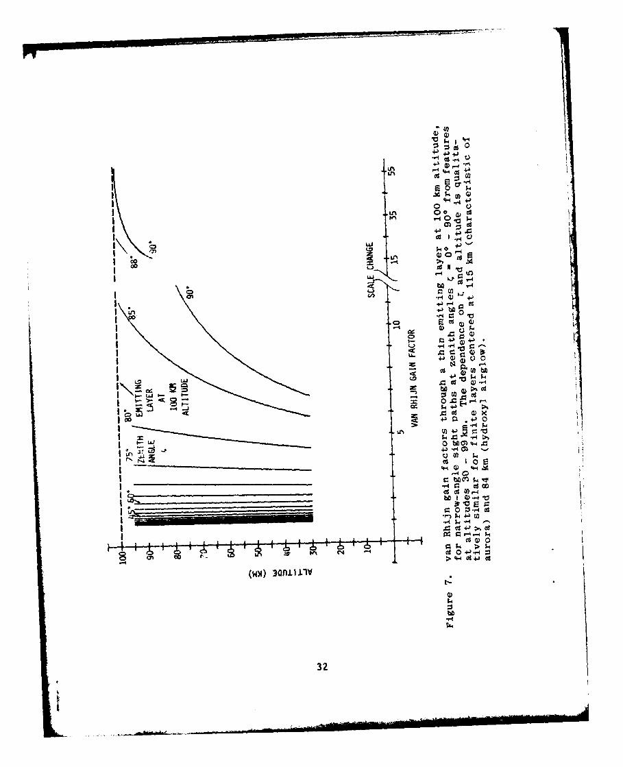
7. Path length gain factors to features below a thinemitting layer at t00 km altitude ....................... 32
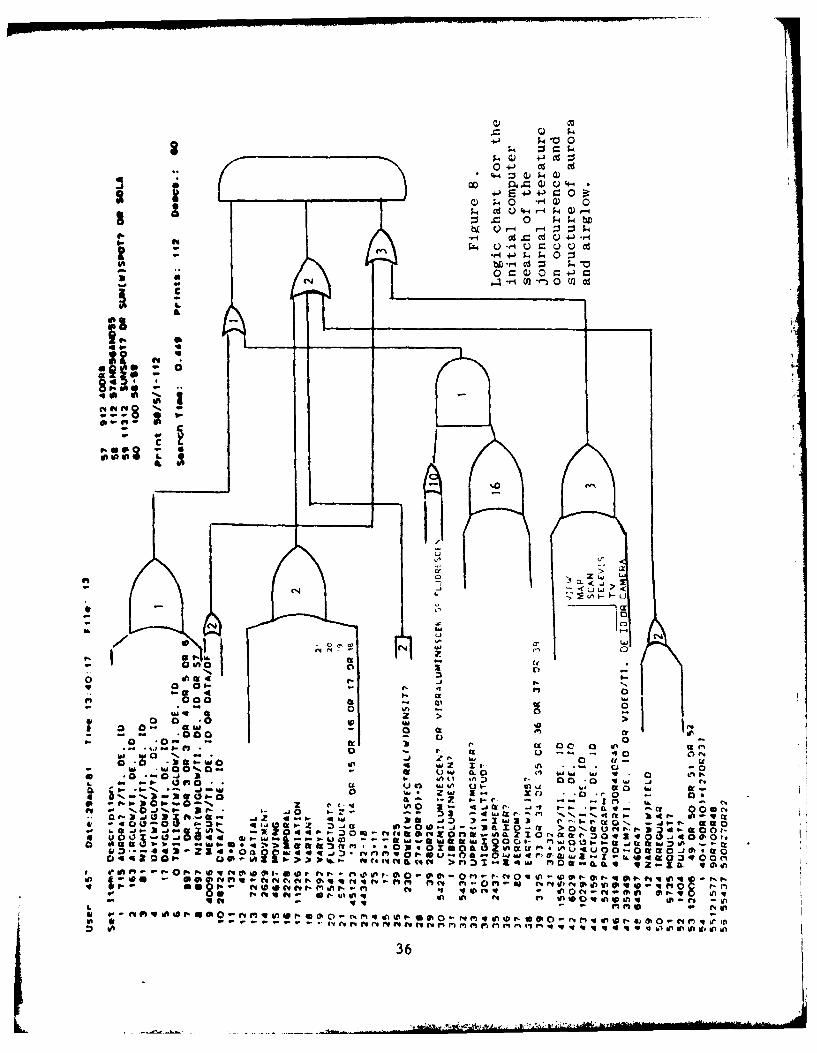
8. Logic chart for the initial computer search of thejournal literature on occurrence and structure ofaurora and airglow .......... ..................... ........ 36
9. Location of the "average" northern-hemisphereauroral oval at 0000, 0600, 1200, and 1800 UT ............ 38
10. Energy deposition altitude profiles for five Max-wellian energy parameters between 0.6 and 10 KeV ......... 47
11. Correlation between total incoming-particle fluxand a) energy parameter, b) altitude of maximumenergy deposition ....................................... 52
12. Fluorescence yields of air at 92-1/2 and 120 km ......... 56
13. Schematic diagram of auroral excitation of nitricoxide vibrational radiation .......................... o... 60
14. Spectral radiance distributions in the nitric oxidevibrational bands excited in aurora ...................... 62
15. Typical wind velocity profiles at auroral altitudes ...... 68
7

ILLUSTRATIONS (concluded)PAGE
16. Altitude profiles of characteristic times for emiss-ion by NO and CO 2 following auroral excitation,and of transport of the precursor species ................ 72
17. Schematic diagram of model of CO 2 4.3om vibralu-minescence excited in aurora ............................ 76
18. Relative spectral radiance distributions in theCO2 v3, NO " (1,0), and NO+' fundamental bands .......... 84
19. Occurrence and exceedance of auroral activity index Q ... 92
20. Plots for transforming geomagnetic to geographiccoordinates ...... ........... . .. .... .... .......... 95
21. Dependence of frequency of auroral activity on Kp ....... 100
22. Estimated probabilities of occurrence of zenithenergy input within the nighttime auroral oval .......... 102
23. Flow diagram for a model of occurrence ofauroral infrared background clutter ..................... 106
24. Mean zenith spectral radiance of the hydroxyl-fundamental airglow .................. ................ 114
25. Flow diagram for a model of occurrence ofhydroxyl airglow background clutter .............. 128
26. Geometry of the hydroxyl radiance variations ............ 134
LIST OF TABLES
1. Scope of Assessment r Auroral/Airglow Backgrounds ...... 13
2. Technical Background on Infrared Aurora and Airglow ..... 17
3. Deposition Profile Characteristics ...................... 53
4. Altitude Profiles of Excitation and Transport of4.3um CO2 Radiation ..................................... 78
5. Expected Properties of Near-Prompt 4.3an Radiation ...... 85
6. Mean Zenith Radiance of Hydroxyl Fundamental Bands ...... 113
8
1. Introduction
We review in this report the existing data base on spatial
and temporal structure of the natural infrared aurora and air-
glow, and specify from this information models of the occurrence
of their radiant intensities and inhomogeneities. Definition of
the global distribution of background clutter from the atmosphere
provides standardized, quantitative criteria for design of optical
measurements systems; specifically, the noise spectrums serve in
selecting the wavelength sensitivity bands, spatial resolution,
signal integration times, background-suppression logic, and
other engineering factors that optimize system performance.
Additionally, real-time prediction of geophysical effects on
the sky's radiance -- in particular, the sporadic increases
and irregularities resulting from magnetospheric disturbances --
would permit future measurements systems to mitigate their
impact by changing operating parameters such as wavelength
band intervals.
Aurora (for the purposes of this report) is the luminosity
of high-altitude air resulting from impact excitation by charged
particles, principally electrons with energy near 5 kilo-electron
volts, that flow into the high-latitude atmosphere from the
magnetosphere. We define airglow to be the other non-thermal,
chemical reaction-indulced radiations from the earth's upper
atmosphere, with the exceptions of resonant and fluorescent
scattering of sunlight and earthshine and of glows excited by
sporadic local events such as meteor trains and lightning strokes.
Unlike aurora, airglow is virtually never detectable by the
unaided eye because of its low radiance and contrast. The
energy source for airglow radiation is short wavelength photons
from the sun, which with their photoelectrons initiate the
reactions by ionizing and dissociating air molecules. Both
91
types of nonequilibriun emission originate from altitudes above
about 70 kin, where photochemistry plays an important part in
determining the species concentrations and the low collision
rates favor depopulation of excited states of molecules and
atoms by emission of ultraviolet, visible, and infrared radiation.
1.1. Context of Auroral-Airglow Clutter Background
The relation of airglow and aurora to the other infrared
backgrounds presented to a measurement platform by the earth's
atmosphere and surface is illustrated schematically in Figure 1.
In the troposphere and stratosphere (<-50 km) the populations of
excited states of the air molecules are controlled by collisions;
that is, the radiational and kinetic temperatures of the gas
are effectively the same. The spectral radiance of this thermal
emission is determined by transport of radiation across the
temperature and species-concentration profiles of the atmosphere.
Vibration-rotation bands of minor permanent-dipole species, in
particular H20 and C02 , play a prominent role in defining the
infrared radiation field (as discussed in Section 1.4). Nadir-
viewing high altitude sensors see also collisionally-excited
radiation -nd resonant and fluorescent scattering from air species
at higher altitudes, and solar photons scattered from molecules
and aerosol at lower altitudes (and at some wavelengths, from
the earth's surface), with an overlay of non-equilibrium molecular
band and atomic line emissions from the upper mesosphere (-70 -
90 km) and thermosphere (>90 km).
As the tangent intercept of the sensor's field-of-view
moves upward, these latter radiations in general contribute a
larger fraction of the signal. The natural spatial and temporal
irregularity of auroral-airglow emissions -- the topic reviewed
in this report -- then plays an increasingly important part in
determining the structure or "clutter" of the total atmospheric
backgro und.
10

I.. CO
fll Nz
c)'~ C.-)
C)C\C/) =M
W4)L
L0QJ uJLLJ
I/ IL -)C
I 4 L I Cf I--
h C)
LL 4J$L 4L )K
= ad C1ck:-

Air Force Geophysics Laboratory has developed computer
models of the spatially- and temporally-averaged infrared spectral
radiances near the earth's limb (Ref 1), and of the lower atmo-
sphere under prespecified meteorological and instrument-pointing
conditions (from LOWTRAN, Ref's 2, 3). These "thermal-emission"
calculations omit excitation by auroral particles and all but
one of the airglow reactions from the physical processes that
populate Infrared-emitting states. The limb model (Ref's 1, 4)
considers resonant and fluorescent scattering of photons from
the sun and earth-lower atmosphere -- which we shall henceforth
include with the collisional excitation -- , and the airglow from
03 molecules in a band centered at 9.6pm (1040 cm- ') produced by
recombination of 0 with 02. Auroral particle input has some
influence on both types of radiation, as aissociation and
excitation of ambient molecules increases the concentrations of
scattering and reactive species such as NO (this issue of effect
of aurora on the "thermal" radiance is not explicitly treated in
this report).
Little information exists on the variability in space and
time of the atmosphere's thermal infrared radiations. We note
that the noise statistics of limb radiances at low and middle
latitudes will be measured under a future USAF program, and that
data on the lower atmosphere's nadir-hemisphere infrared radiance
fluctuations are becoming available from balloon and other high-
altitude measurement platforms.
1.2. Scope of This Report
The scope of the assessment of sky background clutter
reported here is outlined in Table 1. As noted, we review 1)
what we defined above as airglow and 2) the radiations emitted
within a few minutes of the excitation, ionization, and dissoc-
iation of air by auroral particles. We have not considered
12
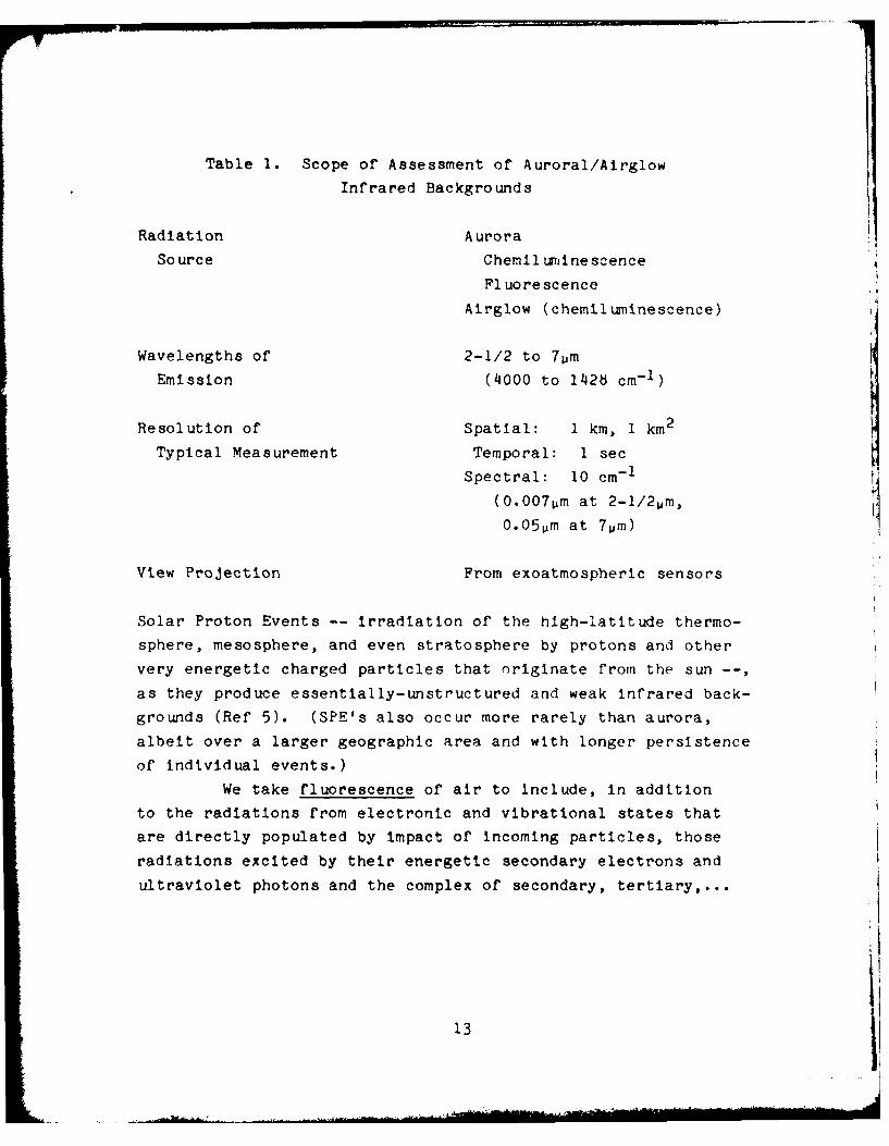
Table 1. Scope of Assessment of Auroral/Airglow
Infrared Backgrounds
Radiation Aurora
So urce Chem ir ine scence
Fluorescence
Airglow (chemiluminescence)
Wavelengths of 2-1/2 to 7pm
Emission (4000 to 1428 cm- )
Resolution of Spatial: I kin, 1 km 2
Typical Measurement Temporal: 1 sec
Spectral: 10 cm-1
(0.O07um at 2-1/2pm,
0.05pm at 7pm)
View Projection From exoatmospheric sensors
Solar Proton Events -- irradiation of the high-latitude thermo-
sphere, mesosphere, and even stratosphere by protons and other
very energetic charged particles that originate from the sun -- ,
as they produce essentially-unstructured and weak infrared back-
grounds (Ref 5). (SPE's also occur more rarely than aurora,
albeit over a larger geographic area and with longer persistence
of individual events.)
We take fluorescence of air to include, in addition
to the radiations from electronic and vibrational states that
are directly populated by impact of incoming particles, those
radiations excited by their energetic secondary electrons and
ultraviolet photons and the complex of secondary, tertiary,...
13
ELI--

processes (recombination reactions, collisional excitation trans-
fer, cascade radiation) that takes place within a few seconds
of the initial deposition of the primary particles' kinetic
energy. (We ignore radiation from longer-lived metastable states,
as in practice it does not contribute to the infrared backgroundclutter.) The W3Au + B3 g (Wu-Benesch) bands of N2, observed
in an EXCEDE artificial-aurora experiment (Ref 6), are an example
of an infrared fluorescence feature from high altitude (low
pressure) air. Fluorescence at the shorter wavelengths to which
the eye and photographic film (and photoemissive detectors) are
sensitive is the most familiar feature of aurora, and is commonly
used to investigate spatial-temporal distributions of particle
input as well as many other aspects of auroral phenomenology.
Chemiluminescence is the conversion into radiation of
the exothermicity of chemical reactions, which in the atmosphere
involve species produced by the action of either auroral particles
or, energetic solar photons. Indirect chemiluninescence can also
take place, the energy of an excited state being transferred
to another atom or molecule. As an example, the reaction of H
atoms with 03 molecules (Section 3) produces vibrationally-
excited OH radicals, which either radiate directly or collis-
ionally transfer their energy (via vibrational excitation of
N2 molecules) to CO2 molecules; which in turn can radiate
at another (longer) wavelength. Chemiluminescence is differen-
tiated from thermal emission by being due to conversion of
chemical potential, rather than kinetic, energy; hence the
initial distribution of vibrational and electronic upper states
does not directly reflect the kinetic temperature of the emitting
species. (Note that in general no hard and clear boundary exists
between chemiliuinescence and the slower aecondary mechanisms
that contribute to what we have called fluorescence, this mild
ambiguity turns out to be of no practical importance.)
14
We have considered only the short- and medium-wavelength
infrared spectral region between 2-1/2 and 7um (wavenumbers
4000-1428 cm-1 ), in which high detector sensitivity can be
achieved with liquid-nitrogen cryocooling systems of weight and
lifetime compatible with the capabilities of certain classes of
measurement platforms. The methods developed here for charac-
terizing auroral and airglow background noise can of course also
be applied to the longer wavelength-infrared features, albeit
with less accuracy because their spectral yields are not as well
known (longward of 15;,m in particular).
The minimum time and space scales of atmospheric varia-
bility and the measurement wavelength interval(s) have been
selected to illustrate conditions of most interest. We consider
a 1 kilometer footprint on the earth's atmosphere (3 x 10- 5 radians
at geosynchronous altitude), and henceforth normalize background
radiances to 1 km2 of radiating area. We take dwell or signal-
integration times down to 1 sec, and spectral widths to 10 wave-
numbers (0.007 and 0.05um "filter widths" at the short- and
long-wavelength extremes of the infrared band considered). This
modest spectral resolution, which is derived from instrument-
design and intensity considerations, reduces the requirements
for extending analysis of the background spectrum to intervals
comparable to the separation between rotational lines in bands
vibration-rotation bands of atmospheric molecules.
The sight paths considered intercept the atmosphere
from satellite orbit, with emphasis on geosynchronous altitude
(5.632 earth radii). While we have not expressly selected the
minimum background-feature intensity that merits consideration,
a reasonable figure based on a comparison to weakly-radiating
man made sources would be 100 watts emitted isotropically into4w steradians from 1 km 2 of projected area, which is about
10 w/km 2 ster.
15

1.3. Overview of Infrared Aurora and Airglow
For further orientation, Table 2 presents a brief out-
line of the characteristics of aurora and airglow that influence
the infrared clutter background, and Figure 2 shows the emission
spectrum measured from a sounding rocket just below the radiating
volumes at a time of intense aurora (Ref 7). The technical issues
In Table 2 will be reviewed quantitatively in Sections 2 and 3.Spatial and temporal inhomogeneity of auroral infra-
red radiance is principally due to the high variability of the
flux of incoming energetic electrons. The spatial gradients
are generally smoothed (and occasionally enhanced) by upperatmospheric winds and turbulence. The emitting air volumes tend
to align along the direction of the earth's magnetic field (as
indicated in Fig 1), since these electrons are constrained
within a few meters of a field line (the Larmor radius) between
their occasional large-angle elastic scatterings by atomic
nuclei. Airglow, on the other hand, results from slow chemi-
luminous reactions following long-period solar ultraviolet
irradiation, and hence the time and space scales of its intensity
changes are considerably longer than those of aurora; the short-
period variability of airglow is due principally to atmosphere-
dynamics. Infrared aurora is limited to the range of high
latitudes from which the particle-guiding geomagnetic field
lines extend into the turbulent (due to interaction of the
solar wind; refer to, for example, Ref 8), charged particle-
releasing magnetosphere; airglow, in contrast, is a global
phenomenon because the effects of sunlight illumination of the
upper atmosphere extend to all latitudes/longitudes. The
vertical-column radiance of aurora varies over an enormous
range; the dynamic range of radiance variability of the major
airglow is only about one order of magnitude at a given viewing
projection.
16
I

Table 2. Technical Background on Infrared Aurora and Airglow
Aurora Airglow
Energy Source Energetic charged Ultraviolet photonsparticles from the from the sunmagnetosphere --continuous input--sporadic input in daytime
Time Delay <0 sec to -50 sec, Hoursbetween Input plus a featureand Radiation persisting >2000 secOutput
Geographic Largely confined to Global -- moreLocation latitudes -100 to 300 variable at high
from geomagnetic poles latitudes
Principal Altitude 90 to 130 km 80 to 90 kmRange of IR (see also AppendixEmission I and II)
Source of Variability of Recurring andSpatial- particle flux latitude-Temporal due to turbulent dependent due toIrregularities interaction of the changes in the
solar wind with sunlight irrad-the magnetosphere iance; episodic
due to atmospheredynamics effectscaused by geo-magnetic storms,stratosphericwarmings, internalatmospheric waves
Range of About a factor 105 ± A factor 3Radiance at latitudes whereVariability particles enter(Approximate) the atmosphere
17
i .....

LrlQ 0Oa, E-4
r. 4) 4- O
II, 00 D
0 -k 0-H4-4 0
o) 0 0 4- Q Q0) 0 C 4)a)o
CNq LA--4 00 0 0.
CLVJ C 0C/) LL Ln a).0 0r4
'-I S- 00a).00'
0 0 C
:> L)L)Q
(.0 W 0 X
0 (12 r..-4 10
0 0 04 2L 0 44)05 4 0
Lu U.) ~-r4 $4 14>C
od N - r- N
LLA 0j 0A E 0>
(WLJ L.)S-LW /S.-( MO1 00
- 9 -- =+C)C no

1.3.1. Emission Spectrum
A low-resolution infrared spectrum of bright
aurora (Fig 2) shows four principal molecular band systems, the
vibrational fundamental (labeled av - 1) and first overtone
(av = 2) sequences of the nitric oxide molecule, the vibra-
tional fundamental of the hydroxyl radical, and the (001-000)
or v3 transition of carbon dioxide. This strong CO2 feature
lies principally between 4.22 and 4 .30um at 200 K rotational
temperature; we shall refer to it as the 4 .3um band. It is inpart due to scattering of earthshine and thermal emission, in
part to the vibrational energy transfer mentioned in Section1.2, and in part to auroral energy input; this last (complex)
process is treated in Section 2.6.2. Fluorescence in severalbands of molecular nitrogen also occurs, and although notresolved in this particular spectrum (being much weaker thanchemiluminescence) was prominent when electrons of energy about
equal to those that produce natural aurora were injected intothe lower thermosphere and mesosphere (Ref 6). Fig 2 indicates
the wavelengths of some of these fluorescence bands, which areemitted within <<l sec after the molecules are excited and thus
closely reflect the inhomogeneities of the initial particle-energy input pattern.
The fundamental (Av = 1) vibrational bands of the
ground electronic state of OH, which lie at wavelengths above2.65um, overlay the NO overtone radiation. These turn out tobe by far the most intense airglow (at any wavelength), and in-
deed the only one so far detected in the 2-7pm region (with the
exception of the O~tH N2t+ C02t. CO2 + 4.3um-photon processnoted above). (The symbols t and * indicate vibrationally and
electronically excited states respectively.) An infrared airglowfrom NO, which is largely unstructured and close in peak limb
19

intensity to our nominal threshold of 10 w/km2 ster, is dis-
cussed In Appendix I. Some other weak (and uncertain) chemilurn-
inescent glows from 03 and NO2 are reviewed in Appendix II.
OH airglow is excited principally between 80 and 90 km altitude,
at least at night when the emission profile of its shorter-
wavelength vibrational bands (in the av =2 and higher over-
tone transitions) can be measured from sounding rockets
Auroral emission arises from higher In the atmo-
sphere. The altitude profile or energy deposition depends on
the energy distribution of the incoming charged particles, and
furthermore the efficiency with which these particles' kinetic
energy is converted to radiation In general varies with altitude.
Therefore the infrared aurora's radiance, in vertical as well
as limb projections, depends not only on the total incoming
flux of energy but also on the energies of the individual
charged particles.
1.4. Comparison of Typical Aurora-Airgiow and Thermal
Radiance Backgrounds
To assess further the potential impact of sky back-
grounds from airgiow and aurora relative to the atmosphere's
thermal emissions, we compare some model nadir and limb spec-
tral intensities. Potential AF measurements systems are in
fact stressed by variability in the scene rather than averaged
radiances such as are presented here. To the extent that the
spatial and temporal fluctuations of the non-equilibriumi
emissions exceed those of the thermal -- as might be expected
from a sporadic phenomenon such as aurora -- a -simple comparison
of' mean background intensities underestimates these emissions'
relative effect.The thermal background from the troposphere and strato-
sphere varies with meteorological conditions, in particular withthe altitude profiles of temperature and water vapor concentra-
20

tion. For example the six different model atmospheres considered
in Ref 2 (LOWTRAN 5 calculations) result in nighttime spectral
radiances spanning almost an order of magnitude. In the day-
time the wide range of input conditions -- solar zenith angle,
earth albedo, and clouds and aerosol, among others -- results in
further variability at the short wavelength end of our infrared
range. Additionally, the spectral distributions within the aurora-
airglow features are subject to some error. In view of the
uncertainties in both specifying mean radiances and characterizing
the variability, our comparison of typical backgrounds should be
considered as only a qualitative measure of the relative contri-
tribution to atmospheric clutter made by the non-equilibrium
radiations.
1.4.1. Nadir Radiances
Calculated nadir intensities of the hydroxyl-
fundamental airglow and a moderately intense aurora are compared
with those of the lower atmosphere-earth's surface in Figure 3.
As will be done henceforth, the backgrounds are plotted in units
of watts per steradian per wavenumber from each km2 of radiating
atmosphere; a wavelength scale is also shown, and units of
w/km 2 ster pm are indicated at key points in the plot. Spectral
resolution is 20 cm - I for the thermal radiations and about
15 cm- 1 for the nonequilibrium emissions.
The auroral particle input in Fig 3 is that which
results in an output of 35 x 109 photons/sec cm2 -column (35
kilorayleighs (kR)) in an air fluorescence feature whose intensityclosely follows the energy input rate, the N2 First Negative
(0,0) band with head at 0.3914pm. This rate of particle
energy input, which is 35 kilowatts/km2 , occurs a few percentof the time at auroral latitudes; roughly 10% of this power isconverted to optical radiations. (The input in Fig 2 was about
150 kw/km 2 .) The radiances in the nitric oxide bands can be
21

WAVELENGTH (uM)
6 5 4 3 2:7 2.5I I I I
+4
6 x io5 W/KM2-STER-M
O+2 - x04
3x 10⁴
C.-,
C 2 LOWER;0/2
ATMOSPHERE 02/H2O,,
~010 0, I
NO &AURR G(35KR 0.3914pM)
FUNDAMENTAL OVERTON 4 x lo
0-2
OH AIRGLOW(ME IN CONDITIONS)-04 I-'.
104 A1500 2000 2500 3000 3500 4000
WAVENUMBER (CM-1)
Figure 3. Infrared spectral radiances in the nadir of themean hydroxyl vibrational-bands airglow, thenitric oxide emissions in 35 kR 0.3914um aurora,and the thermal emission and sunlight backscatter-int of the lower atmosphere (midlatitude summerconditions, 600 solar zenith angle in the daytime(dashed) curve). Spectral risolution of thethermal background is iO cm (LOWTRAN), of theairglow-aurora ^-10 cm- . Note: These arenominal, model values intended to provide asemiquantitative comparison of atmospheric back-ground intensities; refer to the text.
22
taken as proportional to the instantaneous rate of energy in-
put when the input is >-5 kw/km2 , so that the NO chemilumin-
escence spectrums in Fig 3 can be moved up or down for other
such high auroral input rates.
As shown, vertical-column brightness in the NO
overtone sequence is about 20 watts/km2 ster (as described in
Section 2.6.1), and that in the O fundamental is 13 watts/km2 -
ster (Section 3). The thermal radiance distribution was adapted
from the LOWTRAN calculations in Ref's 2 and 4 for summer (warm)
atmospheres, with its daytime segment taken from SPOT radiation-
transfer code calculations (Ref 9) for the sun at a zenith angle
of 600.
The comparability of this (intense) aurora and
(normal mean) airglow to the thermal emission at wavenumbers be-
tween -3400 and 3800 cm-1 (wavelengths near 2 .7um) is one of the
most striking features of Fig 3. Qualitatively stated, the strong
absorption-emission bands of the atmosphere's H20 and CO2 molecules
in this region of the spectrum make the upwardescaping thermal
radiation intensity characteristic of the kinetic temperatures
near 25 km altitude, which are lower than those at the ground
surface. (This important effect is indicated in Fig 1.) Absorp-
tion of incident and backscattered solar photons by these mole-
cules also reduces the daytime radiance of the nadir hemisphere.
At longer wavelengths (lower wavenumbers), the
thermal background is increased by the combination of a larger
Planck blackbody-radiation envelope and the generally-higher
radiating temperature at lower altitudes. An exception is the
4.3um CO2 band, whose effective escape altitude is near the
atmosphere's temperature minimum at 90 km (also indicated in
Fig I); hence the low sky brightness in this band. Between about
2400 and 2800 cm-1 -- 3.4 to 4 .2 um -- most of the radiation
reaching nadir-pointing sensors has emerged directly from the
ground or cloud deck; here the "warm" earth and essentially-
transparent atmosphere enhance the thermal radiation relative
23

103 1 ,
io2
~11
OH
~1O~ NO
10-1
10-1
-I
m
10-4,L
NIGHT
2000 3000 4
WAVSUW (M-1)
Figure 4. Infrared spectral radiance of the atmosphere's
thermal emission at 80 km tangent intercept alti-
tude (from Ref 1) and band-averaged radiances of
nitric oxide aurora (35 kR 0.3914pm) and mean
hydroxyl airglow. The OH limb radiance, whose
spectrum is shown in Fig's 5 and 24, is a maxi-
mum at this intercept altitude. A van Rhijn
gain factor of 10 has been applied in plottingthe NO-band intensities.
24

ra and airglow. In addition the greatly increased
iy-radiation function (it approaches a maximum near lOim)
in much more thermal emission near 5.4um than the NO-
ntal aurora.
1.4.2. Limb Radiance Considerations
In sensor projections that do not intercept
s within a few km of) the earth's surface, those molecular
ons that are absorbed and re-emitted by the atmosphere
the brightest features; that is, the emission spectrum is
,d from the nadir view. Additionally, the increased sight
!ngths tend to enhance the relative intensity of infrared
and airglow, to which (with the exception of the CC 2
ice band) the overlying atmosphere is optically thin, as
id-integrated surface brightnesses in optically-thick thermal
)n features change only slowly with intercept altitude.
We select for an initial corparison of above-
7izon radiances an 80 km tangent intercept (the altitude
sest approach to the earth's surface of a spectrometer's
1-narrow field of view). At this tangent altitude the
ath through the mean hydroxyl airglow layer is a maximum;
ie-of-sight cf course also passes twice through auroral-
)n altitudes. Figure 4 compares model daytime and night-
iermal limb radiances (taken from Ref 1) with nominal,
nber-averaged radiances in the OH and NO bands (the latter
iccompanying 35 kR of 0.391 4 pm radiation). Note the in-
p reversal in the CO2 4.3pm band and the H20 - CO2 bands
.7mm, which are identified in Figure 5.
The thermal background in the -1600-1900 cm-1
-- that is, near 5. 4um -- is three or more orders of
ude below that in nadir projections, and therefore it is
5er large compared to the NO fundamental-band chemilumin-
,. Although the reduction in mean radiance is much less
25
10?
H20 2.66+2.67 Pim
(3770 C1MC5lpDAYNIGHT \,
CO2 2.69+2.77 Pm DAY
(3725 & 3610 CM DA H2 2.73 mi 10-1 about equal NIGH (0
~~~~~~intensities) NIH (3 0C - )
H20 2.66+2.67 Pmi0-4 NIGHT
50 100. 1.50OH AIRGLOW AURORA
W11A -
TANGENT INTERCEPT ALTITUDE ((M)Figure 5. Altitude profiles of radiance due to thermal
emission and sunlight-scattering the the H 0 andCO^ bands near 2.7m (adapted from Ref 1) Te2CO bndsnea 2.7im adated romRef1).Thepl~ts show these backgrounds to be about twoorders of magnitude weaker at auroral altitudesthan at the nighttime hydroxyl airglow altitude.
26
IL
in the 3400 - 3800 cm "1 H20 - CO2 emission region (at least
for the atmospheric species concentration profiles adopted in
Ref 1, which are subject to revision), the aforementioned effect
of sight path strongly increases airglow-aurora's relative con-
tribution to the sky background. The OH radiation is plotted as
more intense than NO because the maximum increase in path length
is higher through the thinner emitting layer (as will be shown
in the next subsection).
The radiance of the hydroxyl layer decreases
slowly with tangent altitude just above its lower boundary at 80
km (as will also be evident from the next subsection), and then of
course goes to zero at its upper boundary. As Fig 5 shows,
collisionally-excited emission and scattering in the H20
bands near 2.7um also decreases with altitude. (The daytime
C02 -band radiances increase slightly to -90 km before
falling off.) By 115 km tangent altitude these thermal back-
grounds are about two orders of magnitude below those values
shown in Fig 4 for an 80 km intercept. As 115 km is near the
niximum of the emission profile of moderately intense aurora,
the auroral 2.7um-band background can be substantially greater
than the thermal background.
We point out once again that these comparisons
refer only to mean sky background intensities rather than fluc-
tuation amplitude within bands of spatial and/or temporal frequency,
and that the thermal radiances vary with atmosphere (and ground-
surface) conditions with the limb subject to particularly
high uncertainty. The model data are intended to put the issue
of spectral intensity of the non-equilibrium radiations into the
context of other infrared backgrounds from the earth's atmosphere.
1.4.2.1. Limb Enhancements
As the distribution of clutter back-
grounds is a strong function of the distribution of sight paths
through the emitting layers, we review briefly the dependence of
27
100
sR
A IRGLOW EMITT INGPs = 80 + R KM LAYERP-87 + R KM
AURORAk\\p- 100 + R KM
~P2= 130 + R KM0.
-ESTIMATE CONSIDERINGATTENUATION BY THELOWER ATMOSPHERE
EDGE OF SOLID EARTH
NADIR
8.68 8.40f 00
8.85 8.81 8.60 8.18 6.37 3.5GEOSYNCHRONOUS LLEVATION \,,NGLE 0
(ENDS) 81.32 6.3II 0 V I
74.0 62.5 41.0 20.4
EARTH INTERCEPT LATITUDE 9 (AURORA)m I I 1%m I I I
77.26 70.4 63.4 59.5 41.0 20..4 0°
MID-LAYER INTERCEPT LATITUDE (P'(AURORA)
Figure 6. Path length (van Rhijn) gain factors for geo-synchronous sensors viewing aurora (100-130 kmemission altitude) and hydroxyl airglow (80-87 km).The projection is illustrated in the diagram atthe top of the graph; the spherical angles X andA' (see text) replace 0 and 4< when the interceptlongitude is not in the sensor's nadir meridian.The dashed line at tangent intercepts just abovethe earth's surface is an estimate that considersattenuation by the lower atmosphere.
28

radiance of optically-thin (non-scattering, non-absorbing) air-
glow and aurora on the projection to spaceborne platforms. (A
detailed treatment for radiometers having finite field of view
below and within airglow layers appears in Ref 10.)
Refer to the diagram in Figure 6, in
which height p is measured from the earth's center and R = earth
radius .6370 km. The ratio of oblique to vertical volume emis-
sion rate-weighted path lengths through a layer is given by the
so-called van Rhijn function (Ref's 10,11). For a sensor above
a uniform layer of thickness P2 - P1 this gain factor is a2[(p + 1~1 ~2 - 1/2
maximum of 2[(P2 + P)/P2 - Pl)] when the tangent altitude
of the sight path is pl - R, that is, when the line of sight
just grazes the layer's lower boundary. The maximum van Rhijn
gain factor of the nighttime hydroxyl airglow, which has an
effective thickness P2 - Pl of 7 kin, is thus somewhat greater
than 80. This multiplier was applied in the estimate of OH
limb radiance in Fig 4. Implicit in this calculation is the
assumption that the altitude profile of volume emission rate
does not vary strongly over the horizontal path, which is
7 x 80 = 560 km. In practice nonuniformity of the hydroxyl
emission profile (discussed in Section 3.4) would be expected
to result in some reduction of the maximum gain factor.
The effective vertical radiating thick-
ness P2 - Pl in intense aurora is about 30 km. The resulting
maximum gain factor, 40, would require uniform particle input
over 40 x 30 km = 1200 km horizontally, which in fact would beencountered only rarely in nature. Because of aurora's spatiallyvariable volume emission rates, and as an 80 km tangent intercept
results in less than the maximum achievable van Rhijn gain, we
applied a path length multiplier of only 10 in estimating the
NO chemiluminescence intensities in Fig 4.
Referring to Fig 6, the latitude *
of intercept at height p of a nadir-meridian sight path from
29

an equatorial-latitude sensor located at distance P from the
earth's center is related to the path's elevation angle o by
tan n - p sin 4,/(P - p cos v)- sin *'/(P/p - cos €7).
Thus
n - tan- 1 [sin 41/(P/p - cos *)].
Also, from the law of sines,
-, - sin- 1 [(P/p) sin o -n.
Similarly, the relation between n and the latitude of intercept
on the earth's surface 4 (again restricting the sight path to
the meridian in the sensor's nadir) is
nf- tan - 1 [sin s/(P/R - cos 4)].
(When p = R the intercept is at the earth's surface.) The path
length from elevation angle n through a (rectangular. uniform)
layer with upper and lower boundaries P2 and ol is- p2 sin 2o)1 /2 - (P2 - p2 sin 2 n)1 /2
when arc sin R/P > o > 0;
2[(p - p2 sin 2A) 1/2 _ (02 _ p2 sin 2 r)1 /2].
when arc sin pl/P > o arc sin R/P;
2(p2 _ p2 sin 2n)1/ 2 ,
when arc sin P2 /P > o> arc sin pl/P;
and 0, when o > arc sin 0 2 /P.
The van Rhijn factor is just this path-
length divided by the thickness of the layer P2 - Pl- In practice
the gain does not double discontinuously when the sight path passes
above the solid earth's surface (that is, when sin A reaches R/P)
because the intervening lower atmosphere attenuates radiation
originating from the back side. When the tangent intercept's
height above the earth's surface is greater than pl - R
(o greater than sin oi/P; dashed line in Fig 6's diagram)
the path length, but not the gain factor, becomes independent of
this inner boundary height. When P sin n - p the second
term in the second equation above vanishes and the gain factor
30

reaches its maximum:2 2 1/2 ( -
2[(p2- Pl ) 1 P2 P l =
2[(P2 + Pl)/(P2 -pl)]1 2 .
Limb brightening factors for model
spherical shell hydroxyl and intense-auroral profiles, projected
to a sensor at equatorial geosynchronous altitude (P = 6.6321R),
are shown in Fig 6 as a function of O, 0 (the intercept
latitude on the earth's surface), and 01 (taken as the intercept
latitude of the auroral emission layer's midpoint). When the
line of sight is tangent to the earth's surface o = 8.680,
* = 81.320, and 0- at 115 km midpoint altitude is 70.40. The ab-
scissa scale in Fig 6 is nonlinear (compressed or (for o) greatly
expanded) near the limb, due to the very rapid change in van Rhijn
factor with latitude when 01 (or 0) approaches its upper limit.
The above equations show that the sight path factor remains high
while the tangent intercept rises through most of the layer, and
then rapidly falls off to zero near its upper boundary. Although
the maximum gain decreases as the layer width P2 - P1 increases,
the range of elevation angles o over which it remains near
this maximun of course increases with P2 - Pl
van Rhijn factors can be readily calcu-
lated from the above equations for satellite orbits other than
geostationary. The area of earth and infrared airglow-aurora
surface accessible to sensor fields of course decreases as the
platform's height P - R is decreased. Note that the intercepts
cut through aurora-airglow emission altitudes at lower latitudes
than those at which they project to ground points; for example,
at ground intercepts near the upper-latitude limit of the sight
path from geostationary stations the infrared clutter would come
from aurora or airglow as much as 110 closer to the equator.
For clarity, the relationships above
and Fig 6 were derived for the longitude of intercept points
lying on the platform's nadir meridian. The equations and the
31
4-4*0
4.30.4J
cdc
4-4
0)
cd v
r-4
I-~w V O ~4r
r.W
0 iO
N 0bO 0) (A b
1 0 S*-4 S0
UJ- 0 o
0).$4 .E4 F4
2C od 4)
441
r-4 32
two lower abscissa scales in Fig 6 can be generalized to include
points on the earth's surface at latitude * (measured from theequator), longitude * (measured from the nadir) by replacing with
a new intercept angle X derived from the simple spherical-triangle
relationship cos X - cos cos *. Similarly, V becomes
cos- 1 (cos #* cos *'), where f' and *" are the latitude andlongitude of the sensor field's intercept on the glow layer.
x or V then replaces or f' in determining the elevation
angle 0, which no longer is restricted to the meridian plane
illustrated in Fig 6.
Figure 7 (from calculations in Ref 10)
further illustrates the impact of oblique projections to the
curved earth on the distribution of sky background radiances
from airglow or aurora. The plot shows this emitting path length
as a function of zenith angle (=* + 0) to the sensor
from surveillance targets underneath a narrow radiating layer at
100 km. The dependence of the zenith radiance multiplier on the
sensor's zenith anglc a:d the target's altitude is qualitatively
similar when layers of finite width are at airglow and auroral
altitudes.
1.4.2.2. Effect of Limb Enhancements on
Backgrounds Distributions
We have presented the rather detailed
atmospheric path-length information in Section 1.4.2.1 because
sight paths play a very important part in determining the pro-
bability distributions of atmospheric radiance and clutter viewed
by spaceborne sensors. The van Rhijn gain factors looking from
equatorial geosynchronous altitude are generally high at the high
latitudes where aurora occurs. In addition the vertical-column
hydroxyl radiance is both uncertain and noisy at high latitudes,
because of the perturbations of the mesosphere caused by magneto-
spheric substorms and stratospheric warmings.
i133 .
..... ....

2. Auroral Infrared Backgrounds
The task of characterizing auroral sky background noise
becomes greatly simplified if the phenomenology of particle
energy-input occurrence can be treated separately from the aero-
chemistry that results in infrared emissions. Input to spatially-
localized regions would first be specified, and then the effi-
ciencies and (equally important) characteristic times for
conversion of energy into individual spectrum features would
determine the atmosphere's radiance distribution. Qualitatively
speaking, the emission inhomogeneities would be those of this
energy input convolved with the time delays and resulting trans-
port associated with excitation of the radiating species.
In practice each infrared output has an essentially linear
dependence on energy input; that is, changes in the atmosphere's
composition during aurora do not measurably alter the spectral
yield or the deposition profile, and furthermore the chemical
reactions leading to excitation of individual radiating species
proceed independently. In addition the disturbance in the
atmosphere does not react back on the disturbance in the magneto-
sphere responsible for the incoming-particle streams. Hence
the two major aspects of the natural-backgrounds question,
auroral phenomenology and radiation chemistry of air, can indeed
be decoupled and considered separately.
2.1. Data Base on Auroral Occurrence and Aerochemistry
Auroral occurrence phenomenology (Ref 12) has long been
a subject of research, principally at institutions located at
high laLitudes. In contrast, most of the existing information
about the chemistry and spectroscopy of auroral infrared results
from work done in recent years by Air Force Geophysics Laboratory.
To ensure that no potentially relevant information on
auroral (and also airglow) occurrence statistics, spatial/temp-
oral uniformity, and excitation of infrared radiations would be
34
omitted in specifying clutter models, we made computer-assisted
surveys of the technical reports on those topics. Figure 8 is
the logic flow chart of our initial search of scientific journals,
which used the Massachusetts Institute of Techno]logy's Computer-
ized Literature Search Service. The data base was the worldwide
open technical literature (INSPEC) on geophysics, atmosphere
and atmospheric optics, environment, meteorology, and planetary
and space sciences, which includes approximately 150 journals,
22 annual publications, and 60 monographs. The strategy of
Fig 8 resulted in 278 and 112 abstract printouts respectively
for the periods 1969-77 and 1978-81. About 50 further reports
were identified from this source with a somewhat different
logic that used the descriptors auroral morphology, structure,
and inhomogeneity (among others). This latter search strategy
was then applied to the National Technical Information Service
listing of 1964-1981 Government-sponsored (largely DoD and
NASA) research, resulting in identification of 154 reports.
This literature search as expected turned up moderately
useful information on the systematics of auroral energy input
and potentially-applicable unanalyzed data (as discussed in
Section 2.8.3.2), but no comprehensive survey of the distri-
bution of input-particle flux and energy occurrence as a
function of geographic coordinates, time, and magnetosphere
conditions. That is, no previous global model of intensity and
fluctuation structure of aurora, or of airglow, was found.
Additionally, no significant new data on upper-atmospheric
infrared radiation beyond those considered in AFGL's current
planning of field and laboratory measurements were identified.
2.2. Occurrence Phenomenology
The concept of an auroral-occurrence region having a
boundary that varies with a readily-measurable geophysical
parameter provides a starting point for defining physically-
35 I
Cco
0 j Cd Cd
-) r=. 4- C) V 0a S. 0 -4 ) 0
$w ..- CU 4-4 -4 k -) -4-~: z. 0,4 .) O C
a N ~-M 0 0+~
I> aLL
@0 44
ftD* -0
* -.
-L CL
at 0j
I- j .q I 0 O
-is 0 000 Do- -JI 0"p.-4~ 2 -cofr
* 4 -g 0. UP &
%- 0. - 0rD ~ ~ . mCtT0i
a.ar-u in i
N 0 V ~ % 00 3&Z P' 0 0mfil r) V.r..34% mt 4 N0 m-~ .3r44 m m0 ~'4 ~ l 0l .f" m 4, I ft 4 ' 9-9bl it' in 1. 0
* uo8 .-... ~ ~ S S @ ~ 0 ~ 36
appropriate, frequency distributions of energy input and
spatial-temporal irregularity.
2.2.1. Auroral Oval
One of the first "occurrence" questions to have
been considered was that of probability of visually- or photo-
graphically-detectable aurora appearing in the zenith as a
function of the observer's latitude and longitude. When this
long-standing problem was addressed by analysis of the spatial
and temporal distributions of visible air fluorescence measured
by groundbased wide-angle camera networks, the occurrence data
were found to be ordered by a statistical construct now called
the auroral oval (Ref's 8,13). This oval is, in effect, the
locus of probability >-70% that >-500 w/km 2 energy input rate
(0.3914um-band brightness >1/2 kilorayleigh) appears over-
head within a 30-min period.
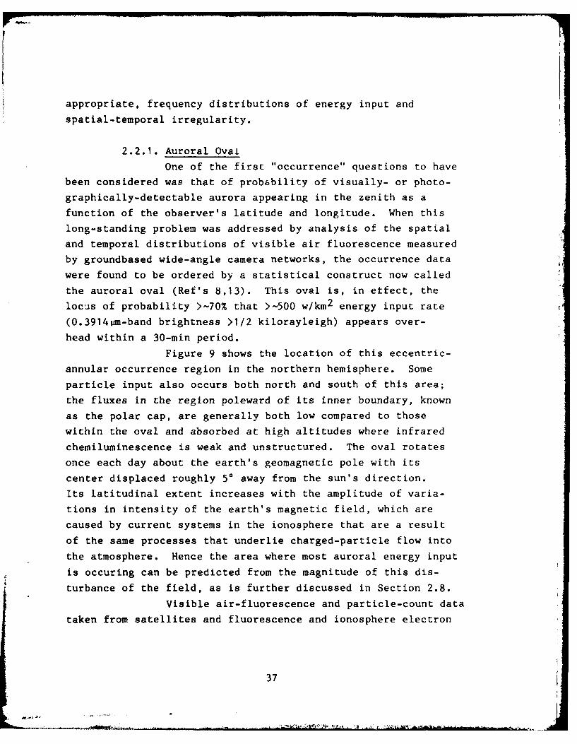
Figure 9 shows the location of this eccentric-
annular occurrence region in the northern hemisphere. Some
particle input also occurs both north and south of this area;
the fluxes in the region poleward of its inner boundary, known
as the polar cap, are generally both low compared to those
within the oval and absorbed at high altitudes where infrared
chemiluminescence is weak and unstructured. The oval rotates
once each day about the earth's geomagnetic pole with its
center displaced roughly 50 away from the sun's direction.
Its latitudinal extent increases with the amplitude of varia-
tions in intensity of the earth's magnetic field, which are
caused by current systems in the ionosphere that are a result
of the same processes that underlie charged-particle flow into
the atmosphere. Hence the area where most auroral energy input
is occuring can be predicted from the magnitude of this dis-
turbance of the field, as is further discussed in Section 2.8.
Visible air-fluorescence and particle-count data
taken from satellites and fluorescence and ionosphere electron
37
-- - a ~4 - .-

OZ LONGITUDE SUN
iT
Fiur 9. " o " io ofth "avrae nortern
Ref 8). VTh eceic"ego rtae
238
ISFigure 9. Location of the "average" northern-hemisphere auroral oval (adapted fromRef 8). The eccentric region rotatesclockwise oncE per day; refer to sectien2.8.2. The geomagnetic pole is shown asa small circle at the center of each mapand the direction to the sun is indicatedwith arrows.
38
,ity data from aircraft (Ref 14) have shown the auroral
.s to be reasonably well-defined regions of diffuse particle
it in which local higher-flux areas are embedded. USAF's
Lr orbiting Defense Meteorological Satellite Program (DMSP'
cles (Ref 15) and the ISIS satellites (Ref 16) have provided
:icularly useful information on the spatial-temporal patterns
Lnput flux and the energy distributions of the incoming
:icles, and imaging photometers on the high eccentricity-
Lt Dynamics Explorer satellite (Appendix III) are now return-
virtually continuous views of the large-scale pattern of
gy input into the atmosphere.
2.2.2. Zenith-Flux Occurrence Probabilities
The oval concept localizes occurrence and leads
:he more pertinent question of the probability of magnitude
he zenith flux at each latitude-longitude. These input-
!nsity probabilities can be estimated from the auroral
-fluorescence and particle-spectroscopy data bases, as
L be discussed in Section 2.8; the currently most access-
a data, which we have specified for the flux occurrences,
from DMSP. The oval's rotation in part defines the diurnal
iation of energy input rate at a given latitude and longitude.
Since the yields of infrared chemiluminescence
I also fluorescence) vary with the excitation altitude,
Dral radiances depend on the altitude profiles of energy
3sition. That is to say, three-dimensional energy input
)ability distributions are needed to determine the sky
Kground in both nadir and near-limb sight daths. Fortun-
Ly there exists a statistical correlation between total
it flux and altitude distribution that allows the profile
3e estimated (Section 2.4.3), which simplifies development
a model of mean volume input rate by eliminating one input
ameter. (Unfortunately, however, as a result of this correla-
39

tion the amount of energy deposited at each altitude cnanges
nonlinearly with the total vertically-directed flux -- it can
even go in the opposite direction (Fig 10); thus the fractional
variations in volume excitation rates are riot simply proportional
to the corresponding irregularities in energy input rate.)
2.2.3. Line-of-Sight Input Occurrence
As the average van R-niJn factor through the
auroral oval from geosynchronous sensors is comparable to its
maximum value (Section 1.4), the horizontal component of the
sight path is typically of order 10 x the 30-km vertical emission
halfwidth or -300 km. In most cases this listance exceeds
the distance over which the particle flux is spatially uniform;
that is, the path length is greater than the characteristic
srale or correlation length of the auroral energy input. Thus
multiplying the zenith energy flux at a specified latitude/
l-ngitude by Its van Rhijn factor (Inside the boundaries of the
oval) 4ould tend to result in too high or too low an input within
the slant-path column. The error due to this broadening of the
d'strbutlon of energy input can in principle be corrected by
aPplying a model of the spatial distribution of zenith flux
along sets of lines of sight.
Intense, discrete aurora -- which is most likely
to degrade exoatmospheric maeasurements of other phenomena -- is
frequently striated with long axis oriented geomagnetically east-
west, that is, about parallel to the oval's boundaries. This
lirect'..nality leads to a qualitatively different pattern of
,ccurreace of energy input within oblique fields of view inter-
secting the auroral layer at longitudes close to and far from
th,? sensor's nadir, as the sight path ri,.y line up with the
striations -- auroral arcs -- at the higher longitudes and
Ir'tersetts several arcs near the nadir. The anisotropy of the
energy input flux's spatial correlation thus makes the probability
dLstrlbutlon of slant coluxnn input change with sensor azimuth
(or longitude angle y) along the air.r'al oval.
40
2.2.4. Inhomogeneity Occurrence
Spatial and temporal str xcture of the input is
statistically specified by power spectral densities (PSD's) of
the particle fluxes. (As noted, the spa 'tal po4er spectrum is
expected to depend on direction relatIve t. tic rval s ooundar-
ies.) Such spectruins usually have a contrnuous frequency 11-
tributlon, which is characterized by an Inner un,,, outer scale,
along with excess power at some characteristic frequencles.
This limited numiber of points would serve to describe numeric-
ally the input Inhomogeneity spectriz,,s. The magnitude of the
auroral flux requires only a single, readily-Intfrcomparable
descriptor.) That is, probability distributions of the amplitude
and frequency at inner and outer scale and of any discrete
Fourier components would quantitatively characterize the stat-
Istics of energy input irregularity.
2.2.4.1. Spatial Inhomogeneity
Analysis of auroral imagery data from
DMSP (Ref 17) is expected to provide information on the spatial
spectrum present In broad (several degrees of latitude or
longitude) input-flux segments in the very near future. Similarly
off-zenith radiance distributions have also been measured with
ground-based photometers, for input to AFGL's "BRIM" procedure
for calculating infrared limb brightness structure (Ref 18).
These appear to be the only available reduced data directly
applicable to modeling the spatial inhomogeneities in auroral
particle flux. (Much more such data exist in elevation-scan
and photographic photometry records from auroral observatories.)
2.2.4.2. Temporal Inhomogeneity
Temporal fluctuations were also meas-
ured for BRIM, but do not extend up to the -1 Hz frequency
41

range suggested in Section 1.2. Several observations have been
ma(ie of large-area quasi-coherent regular pulsations and localized
,illckering of visible aurora (reviewed in Ref 19). The typical
auroral power spectrum, which Is measured by photometers havingboth wide and narrow fields of view, shows a steep decrease with
increasing frequency and often a subsidiary peak indicating a
5-10 sec periodicity (Ref 20). This finding suggests that the
source of auroral particles has natural frequencies in therange of 1/5-1/10 sec - , which has implications in design of
measurements sensors.
We have found no Information relating
temporal power spectrin to the mean energy input rate. Pending
availability of better information, we prescribe using a power
spectrum of the type reported in Ref's 19 and 20 -- (frequency) ~- 3
with a peak centered near 1/7 sec -1 -- to characterize the
temporal irregularity of all auroral particle fluxes. (We
return to this point in Section 2.8.)
2.2.5. Temporal Correlation of Input Flux
As noted, the spatial distribution of auroralenergy input often has a long correlation length, particularly
in the east-west direction, as shown by the existence of optical
forms having nearly uniform brightness extending tens of degreesIn longitude (arcs). Similarly, temporal correlation is evi-denced by the persistence of the patterns of particle input that
produce these forms.
Lifetimes of discrete, intense aurora present
within wide-angle aircraft camera fields (-1000 km diameter
circles) have been found to be Poisson-distributed with a most
probable duration near 15 min (and a weak secondary occurrence
maximum near 120 min) (Ref 21). The average duration of
nearly-constant zenith energy input rate would of course be
shorter, closer to 2 min. Periods of negligible aurora were
42

found to last for typically 20 min or less, but ocrasionally
also extend to 120 min. The 93 hrs of data from this survey
represent an average over the auroral oval and magnetic distur-
bance conditions from near magnetic midnight (which is when the
sun's azimuth is on the night-side of the meridian that pa3ses
through the geomagnetic poles and the measurement point). This
finding of essentially-random occurrence of moderate auroral
activity within areas extending several degrees in latitude and
longitude is supported by a recent analysis of DMSP data (Ref
22).
These activity periods may be compared with the
-1-3 hr duration of the magnetospheric substorm (Ref 8), a
concept that orders many observations of particle- and space
plasma-flux patterns. (At a more fundamental level, it serves
in understanding the interaction of the solar wind with the
magnetosphere that results in release of the auroral particles.)Models of substorm development (Ref 23, for example) call for
systematic changes in the (three-dimensional) spatial distri-
butions of energy input and fluctuation structure in the course
of its half-dozen phases. The -20-min "breakup" phase,
during which the particle energy input is highly irregular in
space and time as well as on-the-average high across much of the
oval, would result in particularly intense and structured sky
backgrounds. (The spectrum in Fig 2 was taken from underneath
what was interpreted as a breakup.)
Adherence to the largely-heuristic construct of
the magnetospheric substorm as the aurorally-active period would
require segmenting the auroral occurrence model to conform to
its phases. On the other hand the development of individual
substorms is so highly variable and unpredictable (as is reviewed
in Ref 22, which makes note of the "types" of substorms
recently proposed), and the spatial-temporal distributions of
43

energy input within each phase so poorly quantified, that this
may prove impractical or even undesirable. Furthermore there
exists the contrary evidence (Ref's 21 ,22) that the lifetimes
of auroral energy input are Poisson-(randomly) distributed --
that is, input does not not follow a predictable course -- ,
about a mean that is substantially less than the duration of
substorms. In consideration of these uncertainties in duration
and systematics of energy input, and the mechanical difficulties
in implementing segmentation by phase, we recommend that the
first-generation model of auroral infrared background omit
explicit consideration of substorm phenomenology.
2.3. Contribution of Protons
Energetic (-100 keV) protons form part of the incom-
ing charged-particle stream, and contribute a spatially-diffuse
component to the optical aurora. Their deposition altitude
profile does not differ greatly from that of the electrons,
with the peak typically between 115 and 130 km. The presence
of protons was initially recognized from the doppler-shifted
hydrogen atom line emissions in auroral spectra, which are
excited when they pick up an orbital electron from the atmo-
sphere's N2 , 02, or 0 to become neutral H atoms. During
the segments of their trajectory that they exist as HO these
particles are unconstrained by the geomagnetic field, which
results in their being Coulomb-scattered about 50 km (root-
mean-square horizontal displacement) before they reach the end
ot their range ; (Ref 11). Thus the distribution of energy
deposition by auroral protons is laterally diffused at a scale
much greater than that of the magnetically-confined auroral
electrons; the spatial spectrum has little power at frequencies
greater than -10- 2 km-1 (other than that due to pre-existing
horizontal structuring of the lower thermosphere's density,
which is small).
The temporal power spectrum of the proton component of
44

auroral input does not exhibtt the -1/10 sec - 1 character-
istic peak and is otherwise lacking in high frequency components.
While under a few daytime-auroral conditions protons carry as
much as half of the incoming energy, they contribute <-i/1C
of the total column excitation in the strong nighttime auroras
most likely to affect measurements systems performance. Thus
protons make only a very small contribution to the time-varl-
ability of the total atmospheric excitation. For these reasons,
the proton flux can be safely omitted from initial treatments
of infrared background clutter.
2.4. Altitude Profiles
Regularities in the altitude profile of energy depo-
sition by the incoming electrons simplify characterization of
the infrared background. Purthermore the statistical correla-
tion between total input flux and range of excitation altitudes
permits construction of a first-approximation model of the
three-dimensional distribution of initial energy deposition
using only one of the two beam parameters.
2.4.1. Particle Energy Distribution
Kinetic energies and pitch angles (direction of
motion relative to the magnetic field) of the incoming auroral
particles have been measured directly from sounding rockets and
low earth orbiting satellites (see, for example, Ref 24). In
many cases the flux of electrons per unit energy can be approx-
imated by a "Maxwellian" distribution E1 exp(-E/a), in par-
ticular at energies E >1/3 kilo-electron volts, which represent
most of the total energy input and the penetration down to alti-
tudes where infrared chemiluminescence is favored. With this
particle spectrum the differential flux is a maximum at the
e-folding energy a (which can be interpreted as the "tempera-
ture" of the incoming electron beam), and the average electron
45*1i-...

energy is 2a. Normalized to a total energy flux F
E d d,/dE) in watts/km2 . the spectrum becomes
do(E)/dE = F x 3.1 x 10¹⁸ ,- 3 E exp(-E/i),
where ds/dE is the downward-directed number flux of auroral
electrons per electron volt (et/sec-eV passing through a
horizontal km 2 from the upper hemisphere) and E and a are in
units of eV.
Altitude profiles of energy deposition in model
upper atmospheres by these auroral electrons have been calculated
from their ionization, elastic scattering, and magnetic-confine-
ment properties. (Ref 25 reviews the various computations, all
of which assume that the incoming and secondary electrons are
not further accelerated by collective atmospheric processes
such as electric discharges.) Figure 10 plots these deposition
profiles for Maxwellian energy distributions with a = 600 to
10.000 eV at auroral latitudes, where the earth's magnetic field
lines are nearly vertical. Note that the 115-km peak altitude
and 30-km vertical halfwidth in the example of limb brightness
enhancements in Fig 6 refer to a .3000 eV. which is characteristic
of moderately intense aurora.
Altitude profiles such as those in Fig 10 are
typical of auroral excitation even when the incoming electrons'
energy distribution departs from Maxwellian. The deposition
rate decreases at high altitudes because the density of the
atmosphere is decreasing, and toward the bottoM side because of
the stopping (and backscattering) of the less-energetic primary
particles.
2.4.2. Optical Diagnostics of the Energy Spectrum
As the auroral beam's cheracteristic energy
decreases (increases) the excitation profile moves to higher
46

-.4 Cd
a) C .-4C4-) F4
-- 4
-)
4-~G
LA.J
-& 4 J2
'.4 - .4 0-
S0
>- >1
__ .-4 w +-
0Za
-C C N C
0 1.4- -4 4
a) xc~~~+ 0 0iD(3N (N -4 -4 -4 4
4 474
(lower) altitudes, where deactivation by collisions is less
(more) probable and the relative concentration of oxygen atoms
is higher (lower). Thus the intensities in emission lines of
0 and bands Of 02 and N2 summed over vertical columns would
be expected to depend on a as well as F. This applies
also to infrared-chemiluminous features, as both the initial
distribution of ionizations, excitations, and dissociations of
ambient species and the subsequent aerochemistry depend on
the relative species concentrations, which vary with altitude.
This principle has been quantified to derive
a for Maxwellian distributions from ratios of near-zenith
radiance of visible auroral features (most notably, in Ref 26)
and nadir radiance in ultraviolet features (Ref's 25,27). (In-
frared emission bands could also be used.) A column intensity
ratio to which a is particularly sensitive and which is readily
experimentally accessible is that of the 0.6300Om line of 0 to
First Negative bands of N2 + (the strong 0.3914 and 0.4278 m bands
provide the best precision). The long-lived metastable upper
state of this red oxygen line is collisionally deactivated below
about 220 kin, while the blue-near ultraviolet First Negative
system, which originates from electron impact on N2 molecules, is
unquenched at all. auroral altitudes.
Radiances in these spectroscopic features measured
from ground stations or satellites -- or from aircraft, which
are more accurate because the corrections for scattering of
auroral photons by the atmosphere are very small -- thus permit
estimation of altitude profiles of the energy input. Both the
altitude and halfwidth of the peak in the profile depend on a.
The maximum volume excitation rate also depends on F, to which (as
noted earlier) the column intensities in the N2 bands are closely
proportional. (Actually the ratio F/(N +-band radiance) depends
somewhat on a because the relative concentration of N2 mole-cules increases toward lower altitudes, a secondary effect that
is taken into account in Ref 26's model.)
48

The Maxwellian distribution of course represents
only a two-parameter fit to what is often a structured differ-
ential spectrum with spikes of mono-energetic electrons, par-
ticularly in discrete auroral forms (see, for example, Ref 28).
It underestimates the number of low-energy ((-300 eV) primaries,
which do not contribute to infrared clutter backgrounds (more
on this shortly) but add to the 0.6300izn-line radiation.
Furthermore the ratios are recognized as a less-than-perfect
measure of a on both theoretical grounds (the input information
on electron energy dissipation, excitation of molecules and
atoms, and atmosphere composition are subject to some error) and
for experimental reasons (photometers may not view excitation by
electron streams in which a is everywhere constant, especially
if they are not pointed along a magnetic field line; and the 0.631Rn
line emission requires -1/2 min of near-constant energy
input to reach an equilibrium emission intensity). Nonetheless,
in large part because of its convenience, the spectroscopic-ratios
method has been widely applied for assessing altitude profiles
of auroral excitation. (BRIM's limb-radiance calculations are
based on it, for example.)
2.4.3. Dependence of F on a
In situ measurements of the free-electron density
and energetic-electron flux are inherently the most accurate
means of determining altitude profiles of energy deposition
rates. Unfortunately, too few such measurements have been made
with the aurora remaining stable in space and time during passage
of the rocket probe to systematize the relationship between
F and a. Particle energy spectrums measured from satellites
are another, less direct source of profile information. However
most of the energy distributions reported refer to individual
auroral events being analyzed in depth, and the results of a
major survey (Ref 29) are not presented in a form directly suitable
49

for conversion to sets of deposition profiles. Furtner, particle-
flux data from sun-synchronous polar-orbiting satellites (such
as DMSP) apply only to the limited range of local times during
which they regularly pass over the auroral ovals.
Still another source is incoherent-backscatter
radar data (Ref 30,31), which refer to narrow ranges of latitude/
longitude across which the auroral oval cuts obliquely due to
Its eccentric rotation. These radar results are subject to some
uncertainty from the conversion of the measured quantity,
ionospheric electron densities, to rates of ionization by the
incoming particles (the same can be said about in situ electron
density mcasurements). Although we have identified no published
Long-period radar survey that focuses on the relationship between
F and a (or for that matter on occurrence statistics of F),
the input data for a comprehensive study are most probably on
record.
An immediately-available data base on energy
input profiles appropriate to systematizing auroral infrared
backgrounds is the ~6000 spectroscopic ratios measured from
a NASA subsonic jet aircraft in 1968-69 (Ref 32). Similar large
sets of zenith-photometry data, as yet unanalyzed, are available
from the 1967-1980 auroral-latitude flights of AFGL's NKC-135
research aircraft S/N 55-3120 (Ref 33) and 55-3131. (These
latter measurements could be segmented by latitude, local time,
magnetic-field disturbance, and even phase of the solar cycle --
and perhaps phase of substorms.) We note also that the imaging
photometers on the recently-orbited Dynamics Explorer Satellite
will provide further systematic information on occurrence
and the F-a relationship when F >_ 1 kw/km 2 over >-(50 km) 2
areas, and that remote optical or ultraviolet sensing from
satellites can provide real-time eetimates of the auroral energy
deposition profile for measurements systems applications, even
In the daytime (as is discussed in Appendix III).
50
The NASA suevey consists of approximately 200
hrs of measurements with 3' field photometers (giving a footprint
of 5 km on auroral erniss-Lon), which were averaged over
2-mmn intervals -'-25 km aircraft motion). Since the sampl-
ings were made over a period ot months at a wide range of auroral
latitudes and geomagnetic times (Ref 34) the data base is a more-
or-less representative sum over geophysical conditions. (Geo-
magnetic time (Section 2.8.2) is reckoned from the azimuth angle
between the sun and the meridian that passes through the geomag-
netic poles and the latitude-longitude to which the time refers.)
F and a were measured from the radiances in the 0.4278im N2 +First Negative band and the 0.6300 mn 0 line.
Figure 11a shows the polynomial best-fit between
F and a (from Ref 32) with the approximate mean range of
scatter in their cross plot (from our estimate). (The data set
remains available for calculation of the correlation coefficient,
which is not given in Ref 32.) The corresponding altitudes of
maximum energy deposition (from Ref 35) are plotted in Figure
11b, which includes for later reference the [0]/(N 2 ] ratio
from the Jacchia 1977 model atmosphere (Ref 36).
The considerable natural scatter indicated in the
plot of F against a is also evident in auroral-particle
spectrums measured by other than optical means (Ref's 23,28,
and 37, for example). The spread in peak altitude of the
profile (Fig 11b), on the other hand, becomes only ±6 km
when F reaches 5000 watts/km2 (5 kR 0.3914 pm radiation)., This
narrowing is due to the increasing effect of the exponential
increase in atmospheric density near the end of the primary
electrons' penetration ranges. Insensitivity to a of the rela-
tive profile at high a and F is also evident in Fig 10, which
plots absolute rates of energy deposition per unit volume
calculated for four a, F on the best-fit regression line in
Fig 11a. Parameters of these profiles are given in Table 3.
51

0.01 0.1 1.0170
160
150
140 /
130 -/O1
120 /X b) /
110
10
S 8 POLYNOMIAL
BEST-FIT
6-LU C a)
4 -MEANm SCATTER
~RANGE
2
LLJ 0 ._ _ .LI I I I. f l l10 100 1000 10,000 100,000
INCOMING PARTICLE ENERGY FLUX F (WATTS/KM2)
Figure 11. Correlation between Maxmellian energy parameter aand total incoming-particle flux F as measuredfrom a survey aircraft by the spectroscopic-ratiosmethod (a), and resulting correlation between F
and altitude of maximum energy deposition (b).
52
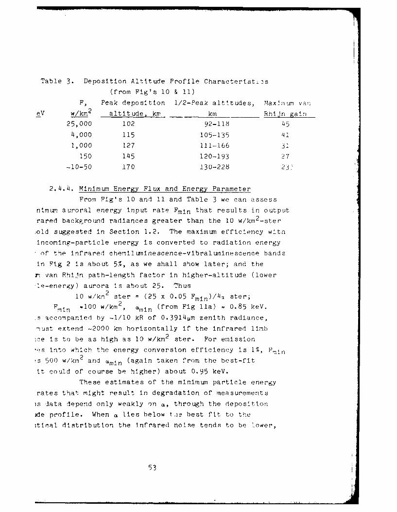
Table 3. Deposition Altitude Profile Characteristics
(from Pig's 10 & 11)
F, Peak deposition 1/2-Peak altttudes, Maximum vani
eV w/km 2 altitude, km km Rhijn gain
25,000 102 92-118 45
4,000 115 105-135 41
1,000 127 111-166 3.
150 145 120-193 27
-10-50 170 130-228 23'
2.4.4. Minimum Energy Flux and Energy Parameter
From Pig's 10 and 11 and Table 3 we can assess
nimum auroral energy input rate Fmin that results in output
rared background radiances greater than the 10 w/km 2 -ster
iold suggested In Section 1.2. The maximum efficiency with
Incoming-particle energy is converted to radiation energy
of the infrared chemiluninescence-vibralumLinescence bands
in Fig 2 is about 5%, as we shall show later; and the
n van RhlJn path-length factor in higher-altitude (lower
le-energy) aurora Is about 25. Thus
210 w/kmn ster = (25 x 0.05 Frnin)/&r ster;
PmIn -100 w/km2 , Ctmin (from Fig lla) - 0.85 keV.
.s accompanied by -1/10 kR of 0.3914pm zenith radiance,
must extend -2000 km horizontally if the infrared limb
ice Is to be as high as 10 w/km 2 ster. For emission
-s into whicb the energy conversion efficiency is 1%, Fmin
!s 500 w/kin2 and umin (again taken from the best-fit
It could of course be higher) about 0.95 keV.
These estimates of the minimum particle energy
rates that might result in degradation of measurements
Is data depend only weakly on a, through the deposition
ide profile. When c lies below t.)E! best fit to the
-tical distribution the infrared noise tends to be lower,
53

u Ln t eonce e.i er iclt g~r~ ~y twr t'~ t~I
ar i h ra (i 1 Ing vo] cznes ar re o r " f- ,a ered" y an 6,: rt of
reaotants. (Tie maxirm r van ,h Jo :,itor a I :.-, r ,
ie r:)asing . ) This means th-,at wnen :s -
-- even r,. erauly larger xt i .- <'-":; I' , .. t
- considered In the model of auroral infrared u5 5.r s
2.5. Auroral Emissions: Fluorescence
hi1e the ;nim r, nput 4Lux rate Is s.me f un2"tion
r -,,rgy 'onversIon yIeld and (secondarily) al. -ttude profiIe
ISection 2.4.4), the minim un scale of iinput irregularlt!es is
wfirned hy delays in emission and the resulting transport ofp o, _rsor species. That is to say, temporal and spatIal fre-
uJincy comTponents of energy input whose effect on the Inf'rared
rii'ance distribut on is strongly attenuated oy the processes
t~tal result In radiation output need not have ,een initially
snecifle. Hence we turn now to the second major Issue in
ur)ra. sky backgrounds, how the emissions are excited in tne
, a ,Ss.ere.
We cor .. er first the less-complex, and less Important,
u,) luor- seence. he auroral particles directly and indirectly
, e a naLiber ult etectronio states of nitrogen molecules,
* *,' ' rnio 1 vely 'and c IIstcnally) cascade wl!rn infrared
.'.',n , Ir s-rv ral han systems. 2-1,/2 - 7P.,, f uorescence
fr.- 'ess-abundant '12 Mrolecules and from 0 atoms is only
,)f te )rer of tne uncertainty in the spectral yields from ,N2 ,
ari "hu. can be neglected. We note for reference that the
U( C' w:ce yield Cron auroral-altitude aiLr in the 0.40 - U. 70km
VV.:hbL-wavelength region (which may include some near-prompt
chem lum .ne,3cer, ce) Is close to 2;.
'Luorescence directly reflect:, the inoomogeneities
of InItial e-nergy deposition at all spatial and temporal scales,
sinr'e it is virtually all emitted within <<I sec of passage of
54

the auroral particles and transmitted by the overlying atmosphere
The low energy conversion yields, however, result in sky back-
grounds below threshold in all but the most intense aurora.
Synthetic spectra that include the 12 most prominent infrared
band systems of N2 and N2+ have been compiled from detailed
surveys of laboratory excitation-deexcitation data and support-
ing theory, for input to atmospheric and auroral codes (Ref 38).
Figure 12 shows fluorescence efficiency per wavenmnber interval
at two altitudes, calculated from this model (in Ref 39) with
the excitation probabilities in one very strong band system (the
W3Au 4 B3 g) increased by a factor 20 from its previously-
accepted value to conform to recent EXCEDE artificial aurortl
measurements (Ref 6). In practice these W + B bands and those of3 3±*
of First Positive (B i g + A3Eu ) sequences largely dominate
dominate the fluorescence spectrum of auroral-altitude air
between 2-1/2 and 7pm. (The steepsided broad peaks in Fig 12
are individual emission bands.) The temperatures in these spec-
trums are those of Ref 36's model atmosphere; the spectral distri-
bution of air fluorescence can be seen to have only a very weak
dependence on temperature at the -5 cm - 1 resolution.
The energy conversion efficiencies plotted in Fig 12
assume a 70% relative concentration of N2 at both deposition
altitudes (79% of all particles are N2 molecules at 90 kin, and
60% at 150 kin). This simplification introduces much less error
than the uncertainties in excitation cross-sections -- of the
W + B bands in particular -- and cascade branching ratios.
Collisional deactivation has little impact on fluorescence
yields above 120 km, and as the spectra show is only about a
factor-two effect at 92-1/2 km deposition altitude. Since only
a small fraction of auroral particle energy is deposited below
-100 km, little error is introduced into most zenith intensities
if the "unquenched" differential fluorescence efficiencies are
used at all altitudes; alternatively the geometric mean of the
55
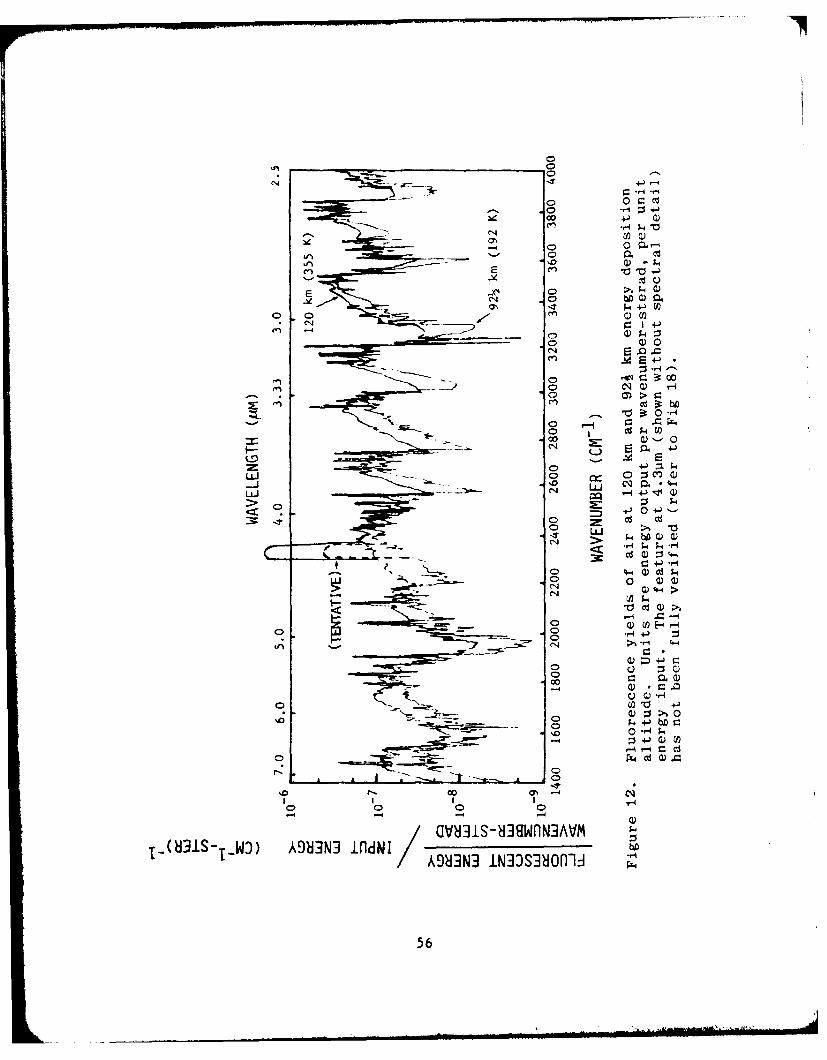
0 r._
-1
0 0.'0) Q)
EE
-CN 0)b
0)
0 n Cd b-
-0 e -or-4
0 --
-4-
-L 0 0
Cd CdLUI >
S00 Q) Q)
r-4 ~
o Q) (0E-.-0n - N 0) * 4-. 4
0 Qo C -
o0 CCL Q.
4 -r4 4
I.- 0--4 r- C * .--
'.0 C- a) C
C))
-44
A9HN3 IN33SJHOlJd
56

efficiencies could be applied. The energy conversion efficien-
cies given are probably upper limits over much of the spectral
range, since the yields in the dominant W * B bands are Incom-
pletely verified.
The ordinate of Fig 12 is in units
Fluorescent energy output _
(kmin column or km3 volume) (waveriumber-sterad)
Particle energy input
(km2 column or km 3 volume)
Sky-background radiance in spectral interval Ak wavenumbers
is then F x (sight path factor) x fuk(ordinate in Fig 12)dk.
As an example, for the reasonably typical conditions of sight
path multiplier = 10 and wavenumber interval 2600-2800 cm- I
(3.57-3.85m filter width; the spiky feature in this interval
is the (3,1) W B band) the fluorescent radiance reaches the
nominal values of Section 1.2 when
F x 10 x -(1.5 x 10- 7 x 100 cm-1 + 3 x 10-7 x 10 cm-1 ) = 10 w/km2 ,
F - 55,000 w/km 2 (55 kR 0.3914om radiation).This figure is indicative of the high input flux levels needed to
produce significant infrared air fluorescence.
2.5.1. "Prompt" Emission near 4.3um
A component of the signal measured by 4.3pm
filter radiometers pointed toward optical aurora from sounding
rockets appears to follow the energy input rates much more closely
than the intense CO2 vibraluminescence-transfer radiation dis-
cussed in Section 2.6.2 (Ref's 40,41,42). This "prompt" radi-
ation has not been identified from its spectrum; prime candid-
ates are NO+ chemiluminescence and impact-excitation of CO 2 .
It Is considered sufficiently well validated from the field
measurements to be included in AFGL's BRIM model.
We have provisionally included this feature
near 4.3um in Fig 12, taking its energy efficiency from the
57

data interpretations in Ref's 42 and 18 (0.3% total yield at
>110 km, increasing deactivation at lower altitudes), and
its spectral width (but not structure) as that of the CO2 v3band at 200 K rotational temperature. Its spectral distribution
would be broadened if this radiation is due to NO+ fundamental
bands; refer to Figure 18 and the discussion in Section 2.6.2.4.
2.6. Auroral Emissions: Chemiluminescence
and Vibraluminescence
As is shown in Fig's 2 and 3, the principal auroral
infrared chemiluminescence is in vibrational bands of nitric
oxide at wavelengths above 2.7 and 5.3un and carbon dioxide
just below 4.3um. The upper atmosphere is optically thin
to NO vibrational radiation, which is excited in reactions that
produce new NO molecules; in contrast the C02 radiation most
copiously produced by aurora, which is in part absorbed and re-
radiated by the atmosphere, is initially excited by transfer
of vibrational energy from N2 to pre-existing CO2 molecules.
The existing data do not rule out the possibilitythat still further molecular species created or initially
present in the atmosphere are chemiluminescing. An upper
limit to the energy yield in any such emissions that are spec-
trally separated from the CO2 and NO bands is -10- 4 , as is shown
by spectroradiometry of aurora and artificially-irradiated air
(in both the laboratory and upper atmosphere). With this low
conversion efficiency the maximum limb radiances of thesefeatures would be near the 10 w/km 2-ster threshold in even the
most intense aurora. Furthermore any such chemiluminescence
would be overlaid by at least comparably intense N2 fluor-
escence, which (as Fig 12 shows) sets a lower limit to the
energy conversion efficiency of about 10-4 per 100-wavenumber
interval -- fairly typical of the spectral width of molecular
bands -- over virtually the whole 2-1/2 - 7wn infrared range.
58

On the other hand the uncertainty in the absolute
yields and spectral distributions of the strong known atmo-
spheric chemiluminescence bands allows for larger yields --
-10-3 -_ in unidentified emissions that would be masked by
these bands. Such radiations would 1) distort the emission
spectrum in and within about 50 cm "1 (-1/I0tan) of the CO2 and
NO overtone bands (less in the NO fundamental, where higher
resolution auroral spectra are available, as described in the
next subsection); 2) superpose further temporal frequency
components on the sky background noise measured by sensors
operating at these wavelengths; and 3) through this change in
time scales, alter the spatial distributions of infrared
radiance. A detailed review of the minor species in air whose
spectrums overlay 2.7, 4.3, and 5.3wm (in the context of
irradiation of the atmosphere by nuclear particles, which
produce more concentrated excitation than aurora and penetrate
to lower altitudes) appears in Ref 43. Since no extraneous
emissions other than (perhaps) the "prompt" 4.31m component can
be considered to be verified, we have not explicitly included
radiation from these molecules in our model of auroral back-
grounds near 2.7 and 5.3um.
2.6.1. Nitric Oxide
The processes that lead to nitric oxide
vibrational radiation in aurora are shown schematically
in Figure 13 (adapted from Ref 41; NO aerochemistry has been
most recently reviewed in Ref 44). The component responsible
for infrared clutter is due to the fast reaction with ambient
02 molecules of N atoms in the low-lying metastable D state.
The resulting vibrationally-excited NO molecules cascade to
the ground state by radiating Av = I or (fewer) Av - 2 photons
and collisions with 0 atoms or (with lower probability) 02 mole-
59
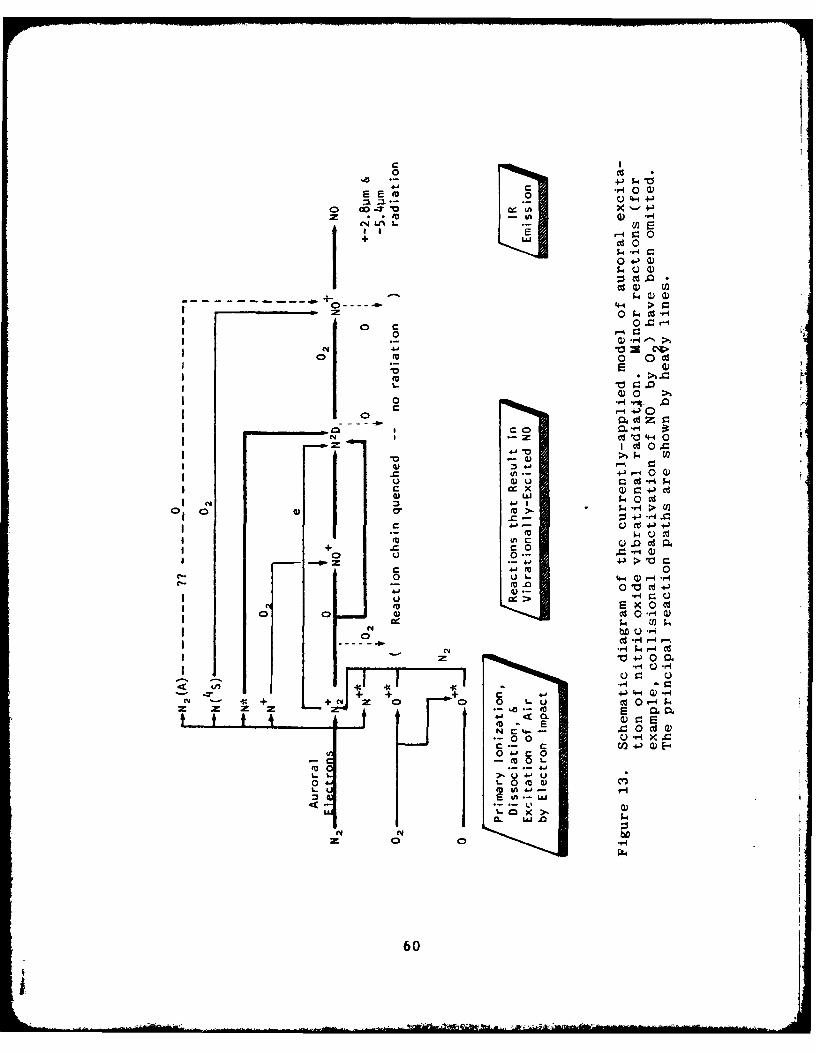
CC
00
E E
o G -T w 0
Z * .0I.
4-4 >,.
0 0 CI 0
I 12a) -ri~
0 0 20 Cd
Q) 0
Cd z -
I Cl
I& N )
0i k 0) 0*
I Cd45 -4 C.)
C-. 0C-.-
c 4. bm 0-I - m VC
-N s. 0 0
+Nd 0 0w -
-- 00o 04.CN CHkr4C
I- '0 -)0U
0 ZOCDU
+- +~4 z -U-40r-
I- 4- E
0 0 -
4-14
60

cules. Since they react much more slowly with 02, ground state
N4 S atoms contribute a longer-lived (-1000 sec), less intense
component that adds little to the background's structure.
The spectral distributions in the NO funda-
mental and overtone sequences, normalized to a particle energy
input flux of 35,000 w/km 2 (remaining constant for >-10 sec),
are shown in Figure 14. (The emission spectrums are higher-
effective resolution versions of those in Fig 3.) These absolute
chemiluminescence efficiencies can be directly compared to the
relative N2 fluorescence efficiencies in Fig 12 by dividing
them by 3.5 x 10⁴; the spectral yields from NO can be seen
to be one to two orders of magnitude higher. They represent
current best-estimates for steady-state auroral excitation,
and are believed to be accurate to within ± a factor 2-1/2
for the fundamental and 1-1/2 for the overtone. Potential
errors of this magnitude arise from uncertainties in absolute
calibration of the rocket instruments (Ref's 45,46), in some
of the rate coefficients for the processes indicated in Fig 13,
and also in the altitude profile of atomic oxygen (Ref 44).
These "equilibrium-excitation" spectrums were derived from the
following experimental and theoretical results.
Yields in the fundamental sequence (Fig 14a)
scale a 180 K rotational temperature laboratory spectrum
unaffected by quenching (Ref 47) to the chemiluminous yield of
2.0% measured in the auroral limb with the HIRIS interfero-
metric spectrometer (Ref 46). (The yield inferred from lower-
resolution zenith spectroradiometry of aurora is 1.5% (Ref 45).)
This spectral distribution is very closely fit by the atmo-
spheric spectrum measured in EXCEDE (Ref 6). Unfortunately
HIRIS's much higher-resolution spectrums cannot be used directly,
as they have a substantial contribution of (1,0) band radiation
from thermal excitation of NO. HIRIS and EXCEDE detect no other
emission features spectrally overlapping the fundamental bands.
61
* ~ ~ ~ ~ ~ i -ik ~$.

0.30FUNDAMENTAL
0.20
0.10 a
L) 1500 1600 1700 1800 1900
0.08OVERTONE
0.06
S0.04
0.02b)
2800 3000 3200 3400 3600 3800
WAVENUM1BER (CM1)
Figure 14. Spectral radiance distributions in the nitricoxide vibrational baud sequences with inputflux F - 35,000 w/km .For direct comparisonwith F'94 12, divide the ordinate scalelby3.5 x 10 . Spectral rejolution 11 cm(fundamental) and 5 cm (overtone).
62
The total energy conversion efficiency into the
fundamental sequence is about half that predicted from model
calculations, perhaps because of quenching or errors in calibra-
tion of the instruments. (These calculations input the initial
vibrational-state population distribution of NO from the reaction
of N2D with 02 measured in the laboratory (Ref 47), the
calculated transition rates (Einstein coefficients) for the
radiative cascade (Ref 48), and the expected number of N2 D
precursor atoms produced along with each ionization.) 2% is the
* best-estimate sequence yield averaged over a - 3 keV auroral
energy deposition profiles.
Although individual NO overtone bands have not
been spectrally resolved in the auroral atmosphere, the total
yield in the sequence is somewhat better known. We adopt an
energy efficiency of 0.7% again averaged over a deposition
profile for a -3 keV. This figure is the mean of measure-
* ments on aurora with with side-viewing (Ref 49) and zenith-
pointing (Ref 45) rocket radiometers and zenith-pointing aircraft
radiometers (Ref 41); it is also supported by calculations using
the above mentioned inputs. The spectral distribution in Fig 14b
is calculated from a radiative cascade model by PhotoMetrics'
AIRSPEC code (Ref 50). Quenching of N2D by 0 atoms, which
lowers the total yield at the higher deposition altitudes (Ref
44), is in effect averaged over altitude in Fig 14. Deactivation
of NOt by 0, which may halve the volume emission rates near the
-100-km peak of the [0] profile (Ref's 43,44), would affect
the relative spectral intensities.
2.6.1.1. Time Dependence
The finite time required for excitation
of NOt results in attenuation of the higher temporal and spatial
frequency components of the auroral-sky radiance in these bands.
Radiometer data from AFGL's aircraft (Ref 51) indicate that the
63
delay between input of particle energy and output of overtone
radiation, averaged over near-vertical measurement columns,
varies between -5 sec and <1 sec. Calculations with the
ARCTIC aerochemistry code (Ref 52) show the zenith radiance
asymptotically approaching equilibrium after a step-function
turnon of the particle beam; the e-folding times are 1-1/2 sec
when a - 10 keV (100 km mean energy deposition altitude)
and 7 sec for 2 keV (120 km), and when the 10 keV beam was
turned off the radiance decreased by a factor e in 1 sec.
BRIM assumes that the final reaction N2 D + 024 NOt + 0
is the rate-limiting step in chemiluminescence, that is, the
excitation process is essentially monomolecular; thus the
characteristic exponential time constant is ([02] x the
reaction rate coefficient, 5.2 x 10⁻¹² cm 3 /sec)- I . This
simplification results in substantially shorter grow-in and
decay times at low deposition altitudes than ARCTIC predicts --
1/10 sec at 100 km and 2-1/2 sec at 120 km -- , as would be
expected from ignoring reaction paths in Fig 13 that do not
involve direct production of N2D by electron impact. Clearly,
assuming that N + 02 is the rate-limiting step gives a lower
limit to the time delay, especially at the lower altitudes
where it is not necessarily slower than N2 D's precursor
reactions.
Volume emission rates can be calcul-
ated by applying a procedure developed in Ref 41, which inte-
grates the energy input backward in time with altitude-dependent
exponential time constants (representing consumption of precursor
species produced at a rate proportional to the input rate).
(BRIM uses a closely similar method.) The procedure is valid
when the scale length of the energy deposition pattern is
larger than the physical transport length, so that thereis negligible net flow of reactants into the emitting volume
64
----------

(as discussed in Section 2.6.1.3). The spectral intensity ot
nitric oxide radiation at time T is then
(Yield from Figure 14/3.5 x 104) x
(I/T) fT exp [-(T - t)/Tl f(t)dt watts/km 3 ster cm -1.
Here f(t) is the rate of energy input at (earlier) time t into
the volume in watts/km3 , which like the characteristic time
T depends on altitude. Typical values of f in aurora with
total input flux rate F are given in Fig 10. To determine
spectral radiances these volume emission rates are summed along
sensor sight paths. This approach could of course be straight-
forwardly modified to take into account the variation with
altitude of the equilibrium yields of NO-radiation, by placing
the yield underneath the integral sign.
The above equation assumes that the
time dependence of NO chemiluminescence can be characterized by
a single exponential time constant, applicable to both its grow-
in and decay, a simplification not completely consistent with
the aforementioned results of aerochemistry code calculations.
Pending further analysis of AFGL's aircraft radiometry data (now
in progress), which will provide further information about
this time dependence, we prescribe the following provisional
values for T. In near-vertical sight paths, a lumped-parameter
figure can be adopted for auroral particle beams having energy
parameter a:
a (F best-fit, from Fig 11) T
> 5 keV O 104 w/km2 1 sec
2 keV 2 x 10³ w/km 2 5 sec
1 keV 3 x 10² w/km 2 50 sec
For calculations of limb radiance:
Energy deposition altitude
< 100 km I sec
110 km 2 sec
120 km 5 sec
135 km 20 sec
150 km 70 sec
65

Clearly, the lower-frequency components in the temporal power
spectrum of clutter background from NO' are attenuated as the
aurora's energy parameter decreases and deposition altitudes
increase. For example, when a = 2 keV the amplitude of
oscillations in infrared output resulting from energy input
pulsating with the "characteristic" auroral period of 10 sec
noted in Section 2.2.4.2 is about an order or magnitude less thaii
the input amplitude. Note also the substantial spread in time
when a <1 keV (alluded to in 6ection 2.4.4), which is accom-
panied by a large spatial spread above the resulting -140 km
peak deposition altitude (Fig ib).
2.6.1.2. Space Dependence
Similarly, transport ot the reactive
precursor species during these radiation times smears out spatial
structure in the NO vibrational-band radiances. Shear in the
upper-atmospheric wind distorts the initial energy-input columns,
and molecular and eddy diffusion spreads the source of emission
vertically as well as horizontally. Although the quantitative
effects of this atmospheric transport are specific to the
geometry of the input distribution and sight path, and in the
general auroral case are not separable from the effects of the
temporal dependence of energy input, its overall impact on the
radiance distributions can be estimated.
The magnitude and direction of the
horizontal wind velocities at auroral latitudes is highly vari-
able, as shown in Figure 15's examples of wind protiles (compiled
from the survey in Ref 53 and data from AFGL's recent Auroral-E
program, Ref 54). Wind shear turns out to be particularly high
near the peaks of the particle energy-input profiles; note the
common occurrence near 120 km of 100-200 m/sec differences
over 10 km vertical distance. The about-average wind speed of
.1 100 m/sec at 120 km would result in -1/2 km (100 m/sec x 5-sect )
66

al offset of the source of NO vibrational radiation trom
itially vertical energy-deposition column. Wind vector
les at auroral altitudes and latitudes have been measured
otography of luminous chemical tracers released from
!ts (as in Ref's 53 and 54) and recently by more-continuous
erent scatter and other (Ref 55) radar methods. While a
-al correlation with magnetic activity is observed, and
-rence and atmospheric-circulation models have been advanced
s 56,57), the wind field can be predicted only statistically.
Diffusion coefficients (Ref 58) and
Lcteristic diffusion lengths of nitrogen atoms at auroral
:udes are as follows:
:itude Diffusion Coefficient D _4D_
) km 102 m2 /sec -- turbulent eddies 20 meters
) km 103 m 2/sec -- molecular 100 meters
) km 3 x 10³ m 2 /sec-- molecular 1/4 km
km 104 m2 /sec -- molecular 1 km
) km 3 x 10⁴ m 2 /sec -- molecular 2-1/2 km.
is the rms horizontal transport distance from an initially-
)w vertical segment in time T. The total spread ot N atoms
:o diffusion would be 2x that shown in the right-hand
in, and diatomic atmospheric molecules (and also ions, such
)+) would be spread V2 x /4DT. The smearing-out of
irsor concentrations due to diffusion changes very little
geophysical conditions, except at the bottom end of the
of auroral energy input altitudes where the variable tur-
ice dominates atmospheric mixing.
Better estimates of the spatial dis-
itions of infrared radiance that result from given time-
Lonary (steady-state) input distributions require detailed
ision-wind drift calculations. Further, when the input
is temporally varying -- specifically, if the scale time ot
67
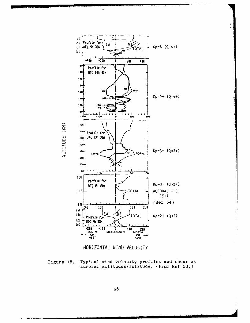
i4 u 'rofile for EW
1,0LI J 5h MmOTAL Kp=6 (Qz6+)
-A0o -200 0 20 400
IG - Profile for160 UT 14h i19
130
Ito -'me- Kp=4+ (Q=4+)
Io=
- 0 -00
10 IGO 20
Profile forLU~~U 1 0 -T13h 30m
e
Kp=3- (Q2+)EW NS TOTAL Kp-(2)
Ito~
-100 0 100 200
120-; -
Profile TOOT IND VEOCT
UT 9 5
Figure 15. Typical
wind velocity profiles
and shear at
auroral altitudes/latitude.
(From Ref
53.)
68
-10 0 10 0

energy deposition rate is less than T -- solution of tirne-depe'W, At
transport equations is required. Note that the chemical reactlo.:
time and molecular diffusion coefficient both chang( in the sar)i
direction with altitude; and that diffusive transport depends
only on VT while the relative displacements by wind shear vary
directly with T and are thus relatively larger than diffus-
ion at the lower auroral altitudes (although the spread is twu-
rather than three-dimensional).
As the energy deposition altitude decre ;.s
-- and most-probable F increasing -- the infrared background
clutter from NO more closely reflects the Inhomogeneities
present in the auroral particle beam. The above tabulations
indicate the temporal and spatial structure of particle Input
that must be considered (or alternatively, neglected) in speci-
fying an auroral model. They show that below approximately
125 km spatial smearing and distortion of the vibrational-radiation
pattern is less than the usual measurements footprint, 1 kin; on
the other hand temporal components down to the nominal minimum
sensor integration time of 1 sec are attenuated at all energy-
deposition altitudes.
2.6.1.3. Spatial-Temporal Radiance Variations
The effects of aerochemical delays
on infrared clutter are sufficiently important to merit re-
emphasis, in particular as they impact CO2 even more than NO
background structure.
Pending availability of more accurate
information, we prescribe calculating volume or column emission
rates of NOt radiation using a single time constant parameter T,
which is a function of altitude or a and independent of the
absolute energy input rate. The average delay in infrared
emission can be shown to be T, and thus the average spatial
offset of the radiation is at the position reached in .
69

Within their expected accuracy these i's do not change with
geophysical conditions. The single-pole linear integrating
circuit will be recognized as an analog of this simplified
aerochemistry model's exponentially-decreasing weighting of
previous input:
R
particle volume or column
energy t(=RC) emission rate of NO
input rate f(t) _ vibrational radiation.
or F(t)
This calculation procedure is physically
valid only when the spatial scale or correlation length of the
energy input is large compared to species transport distances
in characteristic chemiluminescence-output time T; otherwise
net inflow or outflow of reactants from the volumes in the
sensor's field must be considered in predicting their infrared
radiation rates. In those cases that the fractional change in
energy input rate to a specified volume of air is <<I over time
T and the scale length of this input exceeds the transport
distance -- "equilibrium" auroral input in time and space -- ,
Fig 14 directly giLves the spectral yields from that volume.
Aerochemical delay acting independently of mixing damps NO
radiance variations with periods 10 sec at all auroral-
excitation altitudes, and attenuates even 100 sec-period
components of the infrared background at the higher tangent
altitudes.
If the temporal PSD's (power at radian
frequency w) of the energy input F or f are known and mixing-
transport can be neglected, the temporal PSD's of infrared output
intensity can be determined by multiplying this distribution by
the Fourier transform of the atmosphere's response to the input,
(I +w 2 T2 )']. Thus in this auroral case the statistics of
temporal clutter in sky radiance can be straightforwardly
70

assessed. If the correlation length of energy input i.ti so small
that substantial physical transport between a typical senisor's
instantaneous fields of view does take place within time 1, the
temporal frequency distributions in these individual Image
elements (pixels) will be further affected. Calculation of the
infrared radiance distribution in the general case -- aurordl
energy input rate varying In both space and time with scale less
than ~ -requires solution of time-dependent transport equations
with chemical depletion of species (for which a wind field model
must be adopted).
Gradients in the spatial radiance distri.-
bution are reduced by the natural wind shear and (secondarily)
diffusive transport of NOt's precursors during these chemical
induction times, at scales Indicated in the above tabulations
and Figure 16. (While shear and turbulence may also enhance
radiance structure in some view projections, the general tendency
Is toward smoothing.) Charged as well as neutral particles
experience these offsets and spreading, since below -1l40 km
the collision frequency Is sufficiently high to couple the wind
drift and diffusion of the two types of species (that is, pre-
cursor Ions such as NO and N2 are not confined by the geomag-netic field). Variations in the turbulent diffusion coefficient
result in little error in the estimates of physical transport,
because T is small at the altitudes where natural turbulence
occurs. In contrast to the spreading due to diffusion, the bulk
distortions due to wind shear can be predicted only statistically
(except, of course, when the actual shear profile has been mnea-
sured). By analogy with the method mentioned above for calculating
the power spectrum of temporal frequencies in the Infrared back-
ground, the spectrum of spatial frequencies can be determined when
the input spatial spectrum remains sensibly constant for time T by
constructing a spatial filtering function from model wind shear
profiles (as in Fig 15) and the T appropriate to each altitude.
71
Q o C *,.0 bt a-
-4 00i r.O
w0 a
.4-)
rz4zwg (1)Cfl3 ) uW
z72 kQ.0b
2.6.1.4. Altitude Profiles
Figure 16 illustrates in a semiquan-
titative way the effects of aerochemical delays in emission on
temporal and spatial radiance structure from NO and Co
(to be discussed in Section 2.6.2). In the left panel are plotted
altitude profiles of input parameters: VD, a model auroral-
latitude (scalar) wind velocity, and the volume energy deposition
rate f when a = 3 keV (from Fig 10). (Note again the coincidence
of high wind speed with high deposition.) T and the analogous
emission time of CO2 vibraluminescence-transfer radiation, along
with the initial efficiency of conversion of auroral particle
energy to CO2 vibrational energy, are plotted in the middle
panel. The resulting altitude profiles of mean transport of the
two infrared radiation sources are shown in the right-hand panel.
Physically-reasonable values for the "transport length" that
would be applied in the estimation of attenuation of spatial
frequency components of scene radiance alluded to in the pre-
ceding paragraph, can be derived for desired view projections
from these offsets. (For nadir sight paths, for example,
weighting one-half the displacement over the actual particle
energy deposition profile would provide a fair estimate.)
The increase with altitude of the
spatial spread of chemiluminescent reactions works in the same
direction as the decrease in photon yield per initial ionization
(due to quenching of N2 D atoms by 0, Ref 44), both reducing the
power spectral density of sky radiance at the higher spatial
and temporal frequencies. A closely similar effect is found for
CO2 4.3u m-band clutter (refer to Fig 16), 0 atoms again
being the quenching agent. Since the atmosphere above auroral
energy deposition altitudes is optically thin to NO vibrational
radiation (even in very high zenith-angle sight paths), radiance
distributions can be calculated by directly summing volume
emission rate distributions. In contrast, absorption and re-
73
emission of CO2 v3-band photons excited as a result of auroral
particle impact must in general be considered in determining
4.3om scene radiance (as is further discussed in Section 2.6.2).
2.6.1.5. Non-auroral NO Fundamental Band Emission
The vibrational-fundamental cascade spec-
trum in Fig 14a is always overlaid at its high-wavenumber (short-
wavelength) end by thermal emission and earthshine scattering
from the atmosphere's NO molecules in the (1,0) band (Ref's
44,45,46). A midlatitude limb spectrum of this component (at
lower resolution, and on a logarithmic scale) appears in Fig 4;
since [NO] is higher at high latitudes, presumably because of
creation of NO molecules in aurora (Ref's 45,58), the thermal
radiances would be expected to be higher viewing through
the oval. Chemiluminescence in aurora can be looked at as
producing "hot [vibrational] bands" of NO that extend the
thermal background above 5.5um (below 1820 cmn 1). It also
increases the quiescent atmosphere's radiance within the (1,0)
band's spectral range (to the extent discussed in Ref 46) and
adds higher spatial and temporal frequency components to the
infrared noise.
N atoms produced by solar photons also
create NOt, by reacting with 02 molecules at altitudes generally
above the aurora. While this process results in much less
(1,0) band radiation than thermal excitations, it is the principal
source of NO overtone sequence radiation in the dayglow (as
shown in in Appendix I, which also notes that the NO-fundamental
"hot bands" are weak in the airglow).
2.6.2. Carbon Dioxide
Calculation of the background clutter from C02 's
(001-000) 4.3pm resonance transition (the v3 band) is further
complicated by 1) two orders of magnitude longer mean interval
74

between initial energy deposition and infrared emission, 2) a
strong dependence on altitude of the effective efficiency with
which this energy results in vibrational excitation of CO2molecules, and 3) absorption and re-emission ot the radiation
in the atmosphere. To determine surface radiances or even
volume emission rates, coupled sets of equations that describe
the time dependent radiation and excited-species transport
must in general be solved; this is practical for only limited
classes of auroral energy input geometries. Procedures for
approximate solution of the photon diffusion equations (which
do not consider the physical motion of the N2 precursor, which
as we shall see has 4.-portant effects on the radiance distri-
butions) have been developed by AFGL (Ref's 60,61,62) and are
summarized in the description of the BRIM method for calculating
limb radiances in the 4.3um band (Ref 18). As previously noted,
the vibraluminescence of CO2 that results from impact of
energetic charged particles overlies emission excited lower in
the atmosphere by thermal collisions, vibration transfer, and
scattering of earthshine and sunlight (Ref 63); only the
auroral component is explicitly discussed here.
Since the sky radiance distributions from trans-
fer of vibrational quanta are broadly smeared in space and time,
weak "prompt" 4.3um excitation processes could dominate the back-
ground clutter at high frequencies. The important and still un-
resolved issue of other sources of radiation overlapping the CO2band mentioned in Section 2.5.1 is discussed in Section 2.6.2.3.
2.6.2.1. Excitation Transfer and Residence
Times of Vibrational Energy
The collisional and radiative processes
leading to 4.3um vibraluminescence from CO2 are shown in
Figure 17; compare Fig 13 for the chemiluminescence of NO. We
have attempted to make this review of these processes suffic-
75

- a
E IPd
Q) CL -Q- > L
-c4 3 3 E-4
C) t-(N 0
o 0 0V) 0 0'~
z
C,--
0
C) -4N ) )
Co 0 at'
I- WNo~ U ~00
4-4 r.
W 0) Cd
z o-z c
0 CY-nU)" 0 u C) IO
0-4-- c d0
C:4f- J.- (N1-
00
L.&
(N L410 u
76

lently complete to illustrate and provide physical insight into
the proceciures for calculating the radiances from specified
auroral energy Input distributions, and to identify deficiencies
in the information needed to provide usef ul scientific results.
Actual application of these procedures requires substantial corn-
putational effort, and the original sources referenced should of
course be consulted befot'e such calculations are considered.
Table 14 lists characteristic times and
probabilities of collisional energy transfer and direct photon
escape at auroral altitudes. The entries were calculated using
the temperature-dependent chemical reaction rate coefficients
in Ref 6'4, 0 and N2 concentrations from Ref 36's model atmo-
sphere, and the geometric mean of the midlatitude CO2 concen-
trations measured In daytime (Ref 65) and nighttime (Ref 66)
rocket flights. The mass spectroscopically-measured CO2 mixing
ratio (listed in the second column) decreases by almost a
factor 10 between 90 km and 150 km altitude; this profile,
furthermore, would be expected to vary with latitude, as it
depends on the mean solar elevation. Characteristic times
for transfer of energy from N2 tto CO2 (in which the vibra-tional qua-itm is preserved; v-v in Fig 16) and 0 (in which It
is converted to kinetic energy of translation), listed in the
third and fourth columnns, are of course inversely proportional
to the actual concentrations of C02 molecules and 0 atoms
at the latitude of the aurora.
The reactions are Initiated by the
excitation of N2 molecules to vibrational states of their
ground electronic state, principally by secondary electrons
from impacts of the primary aur'oral electrons (thick line in
Fig 17). About 8 vibrational quanta are believed to accompany
each ionization of an atmospheric molecule or atom (somewhat
fewer at the higher altitudes of energy deposition, where the
relative concentration of N2 decreases); this Is an Initial
energy conversion efficiency of 7%, and is considered uncertain
A 77

4- ol
4-
.0 0 0 0 0 0r- C,- 0 0 0
C* 1-4 ~
u ouU - " 0 0 0 0o r-w 0 cD 0 0 0
.,4 EJ4
N o N (
4J~tyo
*r c' u4
oU
o 1-44~
0 4''~ 0 0 ,
H) 0 c.) m :
10 0
> 0
can
00
0 0 .1 ell 0 24- u0 - 0 0 . q
o, - M 0 0 0 0
os W
w 0 C00 0 0 0 w
0 0a0 0 0 0 2
E 0 0 0 0 C 0 c
4.) Go - %. - d . bo
c4 w - cj
E~~~O o ,o*~ ' )
00l 0 u 4o
r0-* 4 t 9 U .lj ...~ 0 0 0 0 #j 1
(S td 0 05 U, C)E *.0 -
> 0 1 0 0 V
'V *6 4
78
because it has not been directly measured. These N2 molecules
transfer their energy in collisions with CO 2 , which are near-
resonant, or with 0 or 02. Below about 80 km altitude the
principal quenching species is 02 (which in turn loses the
vibrational energy in collisions with other molecules); as this
reaction plays a very minor part in determining the 4.3on radi-
ance of the auroral atmosphere it is among those in Fig 17 that
have not been included in Table 4.
The fraction of vibrationally-excited
N2 molecules that excite CO 2 , calculated from the rates of
energy transfer in the third and fourth columns, is given in the
fifth column. By 120 km altitude this fraction has decreased to
1%, so that the effective particle-energy conversion efficiency
is only 0.07%; this shows that vibraluminescence of CO2 is
largely confined to the low-altitude end of auroral deposition
profiles. The sixth column gives the probability that a v3-
band photon initially directed into the upper hemisphere escapes
the atmosphere without further absorption/emission (from Ref 61;
our estimates using the CO 2 altitude profile in the second
column, which is somewhat different from that in Ref 61, are in
parentheses). Those photons initially directed toward the atmo-
sphere's limb -- i.e., in the direction of equatorial-geosynchronous
sensors -- have of course lower probability of directly escaping,
and some of those directed downward are eventually out-scattered
and so contribute to the sky brightness. As is indicated in
Fig 17, some of the vibrational energy is radiated in "weak"
infrared bands: v3 from molecules with isotopic composition
other than C1 20 1 60 1 6 , which have longer mean free paths because
the rotational lines do not line up with those of this most
abundant isotope, and by branching into 9.6 and 10.4 = and
(in part through collisions) longer wavelengths.
The characteristic times for transfer
of the vibrational quantum back to an N2 molecule (seventh
79

column) or other collisional deactivation (eighth column) are
long compared to the radiative lifetime of the CO2 001 state.
0.0023q sec. Hence virtually all the CO molecules excited at
auroral altitudes depopulate by radiating. (At lower altitudes,
the vibrational quantum has a much higher probability of being
transferred by collisions C022 N. CO1 .... or by 4.3um-band
radiation (or collision) CO C0.) The final entry in Table 4
gives the residence time of the quantum (Ref 60), which is in
effect the e-folding time for escape of v3-band radiation from
the atmosphere and so is analogous to the T for exciting NOt
discussed in Section 2.6.1.
This residence time is the inverse of
the sum of the rates of transfer of the quantum of energy from
N2 to
CO2. increased for collisional transfers
back to N2 and corrected for prob-
ability of escape of the photon
from the atmosphere, collisional
quenching of COt, and radiation
in bands other than the 001-000
+ 0
+ 02 (not important at auroral altitudes).
At energy deposition altitudes below 100 km this time is deter-
mined largely by the corrected NJ + Cot transfer rate. The
sharp falloff in IC0 2] above this altitude (Table 4) then causes
the residence time of the quantum to jump to near the time for
its conversion to kinetic energy in collisions of NJ with 0.
-2000 sec. As would be expected, this increase is accompanied
by a rapid decrease in the probability of radiation from CO 2.
and also by near-transparency of the overlying atmosphere to
the v3 -band photons (except in the longer limb paths). The
"ledge" in effective energy conversion efficiency introduces
spatial frequency components near 1/15 km- 1 into the PSD's of
vertical v 3-band radiance (see Fig 16).
80
2.6.2.2. impact on Background of the Con-
version Efficiency and Residence Time
These residence times are of course
)gous to the times required for aerochemical reactions to
te NOt, in that they quantify the duration of intrared
ation output following particle energy input. Since they
two orders of magnitude longer, however, the Nt (and
precursor is moved two orders of magnitude farther
pper-atmospheric winds and spread one order of magnitude
by turbulent and molecular diffusion. As the scale lengths
uroral energy input are usually considerably less than this
sport (typical values of which are shown in Fig 16), surface
ance distributions can only rarely be calculated from a simple
y-time formalism such as was prescribed for NOt, even from
Psition altitudes where the atmosphere is optically thin to
v3 radiation. Wind shear can be expected to smear out
surface radiance spatially as much as the "random walk" of
:on diffusion at all auroral altitudes. (The rms horizontal
!ad from upward-directed 4.3 w photons originating from a
it source at 90 km is of the order of 10 km, and decreases
i increasing altitude.) That is, atmosphere dynamics, which
)nly statistically predictable, has as much effect on the
cground's spatial distribution as radiative transfer, which
least in principle) can be calculated from the absorption-
J parameters and concentration profiles of the atmosphere's
!cules.
Since the probability that the vibra-
ial quantum will be quenched by 0 increases very rapidly
ie 100 km, the energy parameter of the auroral particle
n plays a critical part in determining the CO 2 vibralum-
3cence intensities. Referring to the deposition profiles
Fig 10, we see that little auroral v3 -band emission occurs
a is less than 3 keV. The radiances are obviously sensi-
81
tive to the [C021/[O1 ratio, anti indeed inaccuracy of these con-
centration profiles and in the transport calculations introduces
more uncertainty in the auroral brightnesses than the aforemen-
tioned uncertainty in the number of N2 vibrational quanta initially
excited. (The lifetimes and yields in Table 4 were computed
for midlatitude CO 2 concentrations.)
As noted, quite detailed computations
that include the effects of physical and radiation transport are
required to predict CO2 v3 -band clutter statistics from even
the least spatially and temporally complex auroral energy input
distributions. At present there exists no "library" of results
of such calculations for naturally-occurring structured particle
fluxes in model atmospheric wind and turbulence fields.
2.6.2.3. Other 4.3um Emission(s)
Despite the paucity of such calcula-
tions. it is obvious that this CO2 vibraluminescence-transfer
radiation has negligible spectral power density at temporal
frequencies above -l1- 3 /sec and horizontal spatial frequencies
above -2 x 10- 2 /km (other than that due to horizontal structuring
of the ambient CO 2 and/or 0 concentrations, which is expected to
be small). Again only those inhomogeneities in the particle
energy input pattern having longer time and space scales need
be specified for calculations of the vibraluminescence background.
Such unstructured 4.3um aurora
has been seen by AFGL's zenith-viewing spectroradiometers (as
reviewed in Ref 63). However, the diffuse enhancement seen by
spatially scanning (rotating side- and off-zenith-viewing) fixed-
band radiometers on two of their sounding rockets is overlaid
by a more localized component (Ref's 40,42,67). Additional
evidence for "near-prompt" 4.3urm-band emission is provided
by the EXCEDE spectrums, which show a factor three more radia-
tion than predicted from the times required for vibralum-
R2

inescence transfer (Ref 68). This more closely correlated
emission, should it be verified by subsequent measurements,
would reflect the irregularities in energy input and so repre-
sent a potentially more important source of infrared noise.
Two excitation processes, electron
impact excited fluorescence of CO 2 and chemiluminescence of
NO+ -- currently more favored -- , have been invoked as the source
of this emission (refer to Table 5). NO+t would be excited
in the exothermic reactions following initial ionization of air
N2 + + 0 + NO+t + N and
N + 0 2 + NO+t + 0
and, with less probability
N2 + 0 + - NO + t + N and
NO + O + 4 NO + t + 02.
Characteristic times for completion of the first two atom-
interchange reactions are estimated in Table 5 from their rate
coefficients (-2 x 10⁻¹⁰ cm 3/sec to all states of the
products) and the auroral atmosphere's concentration of 0 atoms
and 02 molecules These time scales are considerably shorter
than those fo NO chemiluminescence, as the rate coefficients
for the ion-neutral reactions are higher than that of neutral N
with 02 (and no intermediate reactions are thought to be
involved). Only insignificant spatial and temporal smearing
of the radiance distributions would result from these short
delays. The measurements to date on artificial (Ref 68) and
natural (Ref's 42,67) aurora did not have sufficient resolu-
tion to quantify the temporal and spatial correlation between
energy input and "near-prompt" 4.3mn radiation(s).
Similarly, existing data do not have
sufficient spectral resolution to identify the radiating species,
Figure 18 shows the calculated spectral intensities (at -11 cm -1
resolution) from each excitation process, normalized to the
83
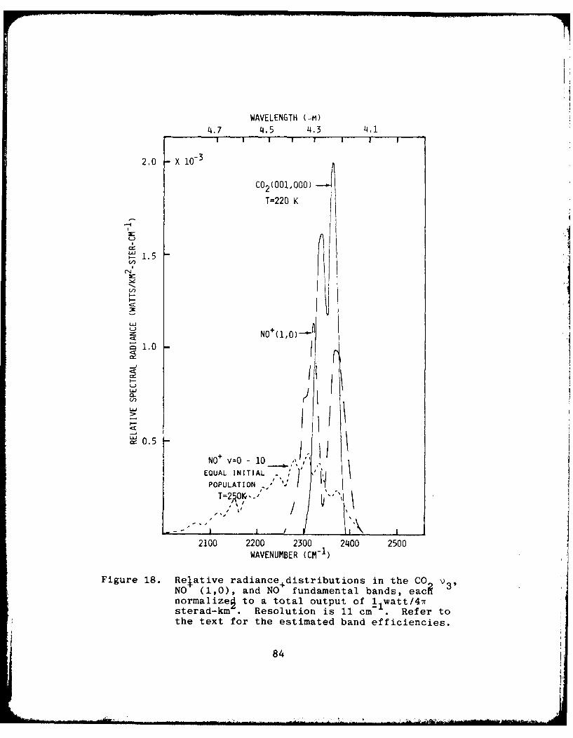
WAVELENGTH (.M)4.7 4.5 4.3 4.1
I I I I 1 I
2.0 X 10⁻³
C02(001,000)
T=220 K
1.LU
CN
NO (1,0)-
~1.0
C
LU
" /~ 05NO += v010 ~ 1
EQUAL INITIAL , '.
POPULATION " - I IT=2RO& , . ",
2100 2200 2300 2400 2500WAVENUMBER (CM-1)
Figure 18. Relative radiance.distributions in the CO_ v3'NO (1,0), and NO fundamental bands, eachnormalizeq to a total output of l1 watt/4Tsterad-km . Resolution is 11 cm- . Refer tothe text for the estimated band efficiencies.
84
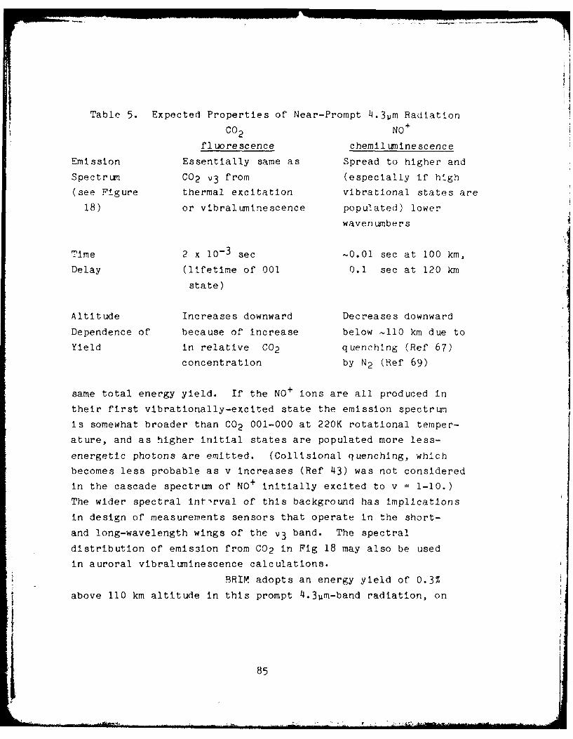
Table 5. Expected Properties of Near-Prompt 4.3pm Radiation
CO2 NO+
fl uorescence chemil ininescence
Emission Essentially same as Spread to higher and
Spectrum CO2 v3 from (especially if high
(see Figure thermal excitation vibrational states are
18) or vibraluminescence populated) lowerwaven umbers
Time 2 x I0 - 3 sec -0.01 sec at 100 kin,
Delay (lifetime of 001 0.1 sec at 120 km
state)
Altitude Increases downward Decreases downward
Dependence of because of increase below ~110 km due to
Yield in relative CO2 quenching (Ref 67)
concentration by N2 (Ref 69)
same total energy yield. If the NO+ ions are all produced in
their first vibrationally-excited state the emission spectrum
is somewhat broader than CO2 001-000 at 220K rotational temper-
ature, and as higher initial states are populated more less-
energetic photons are emitted. (Collisional quenching, which
becomes less probable as v increases (Ref 43) was not considered
in the cascade spectrum of NO+ initially excited to v = 1-10.)
The wider spectral int'rval of this background has implications
in design of measurements sensors that operate in the short-
and long-wavelength wings of the v3 band. The spectral
distribution of emis3ion from CO2 in Fig 18 may also be used
in auroral vibraluminescence calculations.
BRIM adopts an energy yield of 0.3Z
above 110 km altitude in this prompt 4.3um-band radiation, on
85

the basis of radiometry data from 1978 auroral probe IC 807.15
(Ref 67); a figure of 0.2 - 0.5% was derived from the 1974 probe
A18.219-1 (Ref 42). As the time scale of the feature is expected
to be <1 sec (Table 5), we have included it in the plot of air
fluorescence (Fig 12), spread over -70 cm-1 with spectral
detail omitted. The total band yield is estimated as 0.3% above
110 km, 0.1% at 100 km, and 0.04% at 92-1/2 km energy deposi-
tion altitude on the assumption that the radiation is due to NO+ t
being quenched by N2 molecules (Ref 69). The spectral yields in
Fig 18 have been normalized to a total output of (1/4N) watts/
steradian (from a column or volume), so that radiances or
volume emission rates can be calculated for specified energy-
deposition input rates and assumed radiation process. We note
that if the prompt 4.3pm-band component is 001-000 emission
from CO2 some of the photons will be absorbed in the atmosphere,
and therefore the radiative transfer methods alluded to in
Section 2.6.2.2 must be applied in calculating the sky radiance
distributions that would be measured from exoatmospheric altitudes.
Also, If it is from an NO+ vibrational cascade originating
in part below 110 km, the high-wavenumber end of the spectral
distribution will be less intense than shown in Fig 18 because
of preferential quenching of the lower vibrational states.
With an energy conversion efficiency
of 0.3% above 110 km deposition altitude, a limb radiance of
10 w/km 2 ster in the optically thin emission band is reached
when the input flux rate is 1000 w/km2 (best-fit = 1.6 keV).
All spatial and temporal frequency components (above the mini-
mum scales in Table 1) in aurora with mean F >1000 w/km 2 would
be required to specify the sky background clutter in this
spectral feature.
. 7. Specification of Spatial and Temporal Input Structure
The review of infrared air fluorescence and chemilum-
86

inescence in Sections 2.5 and 2.6 indicates the input-structure
information needed for modeling occurrence of clutter back-
grounds. Insofar as the output (radiance) structure is speci-
fic to the input distribution, the upper limit of sky noise that
can be tolerated is not precisely defined (the 10 w/km2 -ster
minimum-mean is a "soft" boundary), and the radiance is sensi-
tive to intercept latitude or spherical angle X (or A-) through
the van Rhijn factor, the minimum power spectral densities do not
lend themselves to a straightforward tabulation. A brief summary
of input requirements, which carries the assumption that inhomo-
geneities need be considered only when the mean auroral-sky radi-
ance is above the aforementioned threshold, is as follows.
Fluorescence of N2 results in weak backgrounds extending
over the 2-1/2 - 7pm wavelength band (Fig 12). As the emis-
sion rate follows the energy input rate with negligible delay,
all the temporal and spatial frequency components must be speci-
fied when the input rate is above threshold. At a maximum van
Rhijn gain factor of 40, reached when 0 is 8.810 - 8.840 and A'
is near 77-1/40 (Fig 6), the radiance in a - 1/2om spectrum
interval reaches 10 w/km2 ster at input flux about 50 kw/km2 .
A further condition here (which of course also applies in com-
puting the maximum brightnesses of the other infrared features)
is that the flux remains at least this high over a - 1000 km
atmospheric path in the sensor field. For other intercepts on
the auroral-emission layer the minimum F at which frequency-con-
tent information is needed will of course be higher, indeed
considerably so at most latitudes/longitudes (as Fig 6 shows).
Nitric oxide chemiluminescence is principally at 5.3 -
6.2um and 2.7 - 3.1 wn (1900 - 1600 and 3700 - 3300 cm -1 ;
details are in Fig 14), with a much higher energy conversion
efficiency. The threshold F is about 2/3 kw/km 2 (overtone) or
1/4 kw/km2 (fundamental) when the sight path is at the maximum
van Rhijn factor of 30; these figures refer to a best-fit a near
87

1-1/3 keV. Again this condition can apply only over a narrow
range of tangent intercepts, with higher thresholds over most of
the auroral oval. At this worst case, temporal frequency com-
ponents below - 1/30 sec - I and spatial frequency components be-
low - 1/3 km- 1 need be specified for input rates greater than
- 1/2 kw/km 2 ; higher frequencies are severely attenuated by
the chemical delay and accompanying species transport. Parti-
cle fluxes above 5 kw/km 2 (best-fit a = 3 KeV), which result
in above-threshold radiances at angles x- > 690, would call for
frequency components below 1/3 sec -1 and 3 km-1 (which would be
reduced to 1 km- 1 , as the minimum measurements sensor footprint
is 1 km). Fig's 11, 10, 6, and 16 and the tabulations in
Section 2.6.1 provide the data for further estimates of the
maximum spatial and temporal frequencies at which power spec-
tral densities of the energy input are needed to predict the
occurrence of background clutter in the NO vibrational bands.
Carbon dioxide vibraluminescence at 4.22 - 4.30pm
has little spectral power at frequencies above 10 - 3 sec - I and
2 x 10 - 2 km- 1 (horizontally) under any auroral input conditions.
As was shown in the previous section, a model of the occurrence
of sky background in the as-yet-unidentified (or validated)
"prompt 4 .3um" emission would require specification of all
frequency components when F > 1 kw/km2 (again, only in the
narrow range of o or x'). If the radiation proves to be due
to NO+, the effect of the decrease in average energy-conversion
efficiency as a increases (because of increased collisional
quenching at lower energy-deposition altitudes) is to be con-
sidered in determining the minimum input flux rate at other
intercepts.
The above figures are intended to establish semi-
quantitative limits to the input structure detail needed for a
model of infrared clutter. They underscore the ideas that the
highest temporal and spatial frequency components needed vary
inversely with the lowest characteristic emission time and that
88
the minimum particle flux that need be included (for a given
wavelength band) depends rather critically on the sensor
field's elevation angle o or its intercept A-. These limita-
tions on requirements serve to guide f uture measurements or
the occurrence and noise spectrums of auroral energy input.
2.8. An Occurrence Model
We proceed now to outline a first-generation model of
the distribution of infrared radiance and Its structure in
measurements sensors' slant-path liies of sight. The sophis-
tication of the model Is commensurate with the scope and quality
of the input data reviewed in Sections 2.2 (probabilities of
particle energy input) and 2.5 ani 2.6 (aerochemistry and
atmospheric transport). It.--an of course be refined as better
input information becomes available from new measurements
and analysis of existing data bases.
We take the auroral oval (Section 2.2.1) to be the
locus of occurrence of all particle energy input fluxes that re-
sult in above-threshold sky background. The latitudinal extent
of this region can be determined from the measured magnitude of
the disturbance of the geomagnetic field, as described below.
Real-time as well as historical data on these field variations
are available. In addition, the probabilit'cs of Input flux
intensity are also taken as varying with the magnetic distur-
bance. That Is to say, both the spatial location of occurrence
of aurora and the absolute probability distribution of auroral
particle input within this occurrence region are assumed to cor-
relate with the change in net magnetic field at the earth, and
to depend on no geophysical parameter other than local (mag-
netic) time.
Before proceeding, we point out that the "1auroral oval"
concept is somewhat arbitrarily defined (refer to the discussion
89
in Ref 70) in terms of probability of appearance of diffuse par-
ticle fluxes generally well below those that excite above-thres-
hold infrared noise, and that some energy input occurs outside
its boundaries. Nonetheless, insofar as it contains the regions
where discrete areas of high flux are most probable (Ref's 14,71)
and the occurrence of these higher fluxes is roughly proportional
to that of the weaker flux component (Ref 72) (with the proportion
increasing toward the equatorward edge (Ref's 72, 73)), the oval
seen in groundbased all-sky and meteorological satellite images
represents the optimum geometry for a first-generation model
of auroral infrared sky backgrounds.
2.8.1. Auroral Activity Index
The variations in the earth's field are routinely
rmieasured with magnetometers at stations worldwide and applied
to form several numerical descriptors of the level of magnetic
"activity" (Ref's 74, 75, 76), the best known of which is the
global (subauroral-latitude) index Kp. The Auroral Activity
Index (or Polar Range Index) Q has been found to provide a good
statLstical prediction of the extent of auroral particle input
(Ref's 77, 78), as has the AE index (Ref 79). We choose to
apply Q to characterize the oval because it is more commonly
used.
Q is a quasi-logarithmic expression of the maxi-
mum deviation of one horizontal component of the earth's magne-
tic field at auroral latitudes (Ref 75). It is intended to mea-
sure currents in the ionosphere near the station, which have
less effect on the vertical component of the field vector. As
might be expected, Kp and a Q derived from a series of western-
hemisphere stations are statistically correlated (Ref's 34, 80;
they also have nearly equal nunerical values), despite the fact
that the two disturbance indexes refer to different latitudes
90
and possibly field directions. N werical values of Q extend
from 0 (410- 3 fractional change in the field) to 9 (-10-1)
and in very rare cases higher. The dimensions of the auroral
oval shown in Fig 9 refer to Q = 3, a nominal "average" magneto-
spheric-disturbance condition. As a typical time scale of
change in particle-input activity is of the order of 1/4 hr,
an ideal Q would be calculated from the excursions of the
magnetometer signals four times each hour.
Probabilities of occurrence of Q at a single
auroral-latitude station and the distribution of duration of
periods over which Q exceeds fixed values are shown in Figure 19
(from data in Ref 81). Just after solar minimum the Q-indexes
cluster around 2, while after solar maximum they become spread
to higher values. The systematics data in Ref 81 and the monthly
and yearly Q averages listed in Ref 82, along with data on
occurrence and persistence of Kp (in surveys such as Ref 83),
would be used to determine the statistics of oval size and flux
occurrence. "Instantaneous" oval locations can be found from
15-mmn Q indexes reported by civilian agencies.
2.8.2. Dimensions and Location of the Occurrence Region
The boundaries of the auroral oval, which our
model considers as hard-edged limits to the input-occurrence
region, are located in so-called corrected geomagnetic lati-
tude - magnetic local time coordinates (Ref's 78, 84, 85). The
average equatorward geomagnetic latitude OE is fit to a pre-
cision of about 1/20 by a simple analytical expression (Ref 78)
OE = 72 - 0.9 Q - 5.1 cos (H* - 12),
where H* is magnetic time in degrees measured eastward from mag-
netic midnight (defined in Section 2.2.5; H* and its relationship
to geomagnetic longitude ,' are described further in 2.8.1.1)
and the other nunerical quantities in the formula are in degrees.
91

100
80
LL)60LW U
a- DURATION OF
C2) EXCEEDANCEA\
1 HR (AVERAGE OVER
20 H SOLAR CYCLE)
Q_ 24HR
(b)
40 .
k--SOLAR MINIMUMo3 + +3YEARS
o30U
-U
<= C'20
al 0 gSOLAR MAXIMUM + 3 YEARS
10 - C
(a) W 0 0
AURORAL ACTIVITY INDEX Q
Figure 19. Probabilities of occurrence (R.) and distri-bution of duration of exceedance (b) ofauroral activity index Q
92

Thus the outer boundary of occurrence is represented by a circle
around a rotating center offset 5.10 from the geomagnetic pole
(in the direction away from the sun), whose radius increases by
0.90 of latitude per unit Q.
The poleward boundary Op does not depend on
Q in such a simple way, and in addition its center is offset from
that of the equatorial boundary. The data from all sky camera
and meteorological satellite images can be fit (Ref 84) to <10 by
OP =90 - JI - J2 cos (H* + J3 ) ,
where the parameters J(Q) are (again in units of degrees)
Q J1 12 J3
0 15.2 2.4 12
1 15.9 2.7 11
2 16.1 2.5 7
3 16.2 1.9 0
4 16.3 1.4 -4
5 16.4 0.8 -9
6 16.7 0.4 -13
(7 16.8 0 -17)
(8 17.0 0 -21).
The figures in parentheses for Q 7 and 8 are our extrapola-
tion of the results of Ref 84, which presents higher order
parameters for an improved fit to the data. To within the
expected accuracy of our model the extrapolation to higher Q
should be adequate and a closer fit is not justified.
In this regard, we point out that the mean
equatorward boundary of the "diffuse-appearing" aurora in
meteorological satellite images has a scatter of ±21 when
plotted against Kp or the magnetic-disturbance index AE (Ref
79). Hence a more conservative backgrounds model would increase
the area of occurrence by lowering the constant term in the
expression for OE by 20 (to 700) and the J1 's In * p by 10.
93
2.8.2.1. Conversion to Geographic Coordinates
and Universal Time
Corrected geomagnetic latitude-
longitude and local time (which is related to longitude) firn
a natural coordinate system for aurura] occurrence. Measure-
ments sensors, on the other hand, could also be expected to
operate in geographic latitude-longitude and Universa Time.
Hence a conversion between these two coordinate systems is
needed to determine the range of -, ' over which intercept
paths through altitudes where infrared emission can take place
pass within the region where energy input occurs.
in practice this coordinate trans-
formation has been done principally by analog nethods (suchas in Ref 85), as the earth's magnetic field's large departure
from a simple dipole at high latitudes requires tedious corm-
putations to achieve even ±1/20 precLsion. Indeed, we have
not identified In the literature a digital subroutine suitable
for immediate adaptation into an occurrence model. A look-up
zable of suff'icient accuracy can be complied from tne latitude--
longitude plots in Figure 20 (taken f'rom Ref 86) or the analog
auroral-oval plotter in Ref 85. (Such a table is currently in
use at Air Force Geophysics Laboratory (Ref d7).)
Geomagnetic local time ri , tne ihour
angle between the magnetic meridlan y* and the antl-subsolar
(or midnight = noon + 12 hrs) magnetic meridian y, requires
similarly tedious (albeit conceptually simple) computations.
Since the position of the sun moves relative to the pole at a
':ixed local soU±- time H, H* depends on day of the year, .nd
hence on the solar declination, which is tabulated in ephemerises
such as Ref 88 (and also Ref 133). H* can be calculated using
the look-up table, as described below, or found by the analog
method of Ref 85. Alternatively, after ,* of the desired in-
tercept point has been looked up, it can be determined from the
equation (adapted from Ref 89)
94
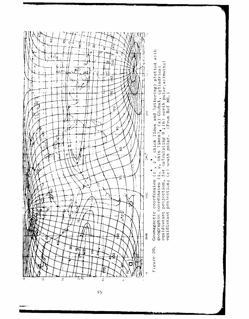
b4
cd
0 w7Z 0 ::r- E
cd .0
C) Ua d
LoQ)
"C5
C 0
4 4-
ct Ld4 4-3
Cd
Cd
0, rz: bLO0 0
bp
N
95

AD-A130 468 INFRARED RADIANCE TRUCTURE OF THE AURORA AND AIRGLOW(U) PHOTOMETRICS INC WOBURN MA I L KOFSKY ET AL.30 JUN 82 PHM-TR-82-02 AFGL-TR-82-0220 F19628-80-C-D134
UNCLASSIFIED F/G 4/1 NL
ENDE
883

L32
11111 1111.6
MICROCOPY RESOLUTION TEST CHART
NATIONAL fiU~ftJ)A ()I SIANVARD~ 9f, A

150 30
30
966

270E
21040 330
80
90I70
97

H* 0 _
sin-1 [cos(Dec)sin U/{1 - (alsin(Dec) - a2cos(Dec)cos U)2}1/2
Here (Dec) is the solar declination angle and U = * - H + a3 ;
H and * are posit.ve eastward, in degrees (H(*) is found from
UT as described in Section 3.2.7). The constants, which are
derived from the latitude and longitude of the geomagnetic
axis poles, are
Northern hemisphere Southern hemisphere
a1 0.984 0.961
a2 0.174 0.276
a3 810 2340.
H' at a given UT and ** (from the
look-up table) can also be determined by locating the geographic
coordinates of the overhead sun (from an ephemeris) and findingI#: + 12 hrs through the look-up table. First the subsolarpoint's longitude (local noon, = 15'(UT - 12)) and latitude (from
the ephemeris; absolute value always < 22-1/2 ° ) are found,
and then the geomagnetic coordinates of this subsolar point are
looked up (in a compilation from Figure 20a). Then
H' = ** - *o = *' - (geomagnetic longitude of noon) + 12.
These He's, or alternatively the *''s(H*, UT), serve to locate
the poleward and equatorward latitude boundaries of the auroral-
input region.
The procedures described here lend them-
selves to digital implementation. Although they may not repre-
sent the optimum strategy for a clutter model, their develop-
ment illustrates the mechanical problems and serves as an intro-
duction to the literature on conversion between geomagnetic
(auroral-occurrence) and geographic (measurements-systems)
coordinates.
2.8.3. Occurrence Within the Oval
As was pointed out in Section 2.2, probabilities
98

of line-of-sight occurrence in near-limb paths at all directions
* relative to the local geomagnetic latitude lines (or oval
boundaries) are needed. We look once again at the existing
data to determine how closely this input requirement can be met.
2.8.3.1. DMSP Images
The most useful reduced data on fre-
quency of occurrence of column energy input come from the Defense
Meteorological Satellite Program (Ref's 15, 17). These polar-
orbiting, sun-synchronous satellites build up images of the
visible and near-infrared air fluorescence from a raster scan
traverse to their -800-km orbital path with a nominal resolu-
tion of --2 km at the nadir and ±560 (-2500 km across)
angular field.
About 750 DMSP images containing both
oval boundaries were analyzed for auroral "activity" as a func-
tion of Kp (Ref 90). In most of these data H* - 0-2 hrs at
the spacecraft's nadir, and all are from winter months (when
scattered sunlight does not obscure the fluorescence). A quali--
tative activity-classification scheme was applied, which with
the help of the DMSP calibration in Ref 91 can be made semi-
quantitative. The results, which apply to the oval as a whole
rather than individual vertical columns, are summarized in Fig-
ure 21. The classification Quiet means that the input fluxes
are well below nominal threshold. Moderate means presence
of some discrete auroral structure with column intensities up
to a few times the mean shown. The Active category includes
scenes with high brightness over most of the longitudinal seg-
ment of oval within the radiometer's field of view, some of
them overexposed in the the photographic reproduction of the
sky brightness distribution. (Some of the DMSP image data are
also available in digital form.)
99

0 4
d ho
A) -A_/> U-H aa 0)/4 Q 0 4
0 ~~ *~ Q.
N I
0 a 0
/~ v~ 0
4qU 43) 4-1
0 4-)
5t-- P4 0a
P.4
(IN33H3d)A1I1IlVOd 33NUM~f33O
100
It is clear that this analysis gives
only very low resolution information about large-area, much
less localized, occurrence of energy input. The intensity re-
solution within the Active category can be improved by apply-
ing the results of a study with a groundbased high-sensitivity
video camera of discrete bright forms (narrow arcs) when Q was
between -3 and 6 (Ref 92). About an order of magnitude
more 104 - 105 w/km 2 events were observed in the magnetic
zenith than l05 - 106 w/km 2 events. (The fact that fewer 103 -
104 w/km 2 events were reported is most probably an artifact of
the sensitivity of the camera and the definition of a discrete
auroral feature.)
2.8.3.2. Other Data
None of the other surveys of auroral
particle fluxes, air fluorescence distributions, or ionospheric
electron densities have been analyzed to produce directly-applicable
data on probabilities of energy input.
The following data bases contain input-
occurrence information, of varying degrees of spatial and inten-
sity resolution. (The references are intended to identify the
data sets, and discuss other results from the experiments.)
--DMSP particle spectrometry (Ref 24)
--000-4 particle spectrometry (Ref 73)
--ISIS particle spectrometry (Ref 93)
--Injun-5 particle spectrometry (Ref 29)
--DMSP images (Ref's 17, 79, 84, 90)
--ISIS images (Ref 71)--Dynamics Explorer images (Appendix III)
--All-sky camera images (Ref 84; also Ref 13)
--S3-4 Satellite UV photometry (Appendix III)
-- Aircraft photometry (Ref's 32 and 33).
101
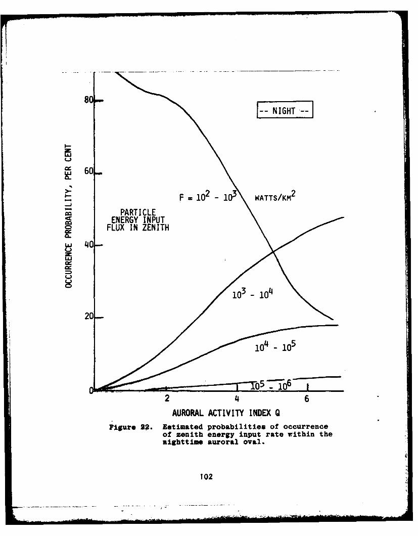
S60,
F 10i2 10 WATTS/KM2
PARTICLEENERGY INPUT
CD FLUX IN ZENITH
w40-
20
2 4 6AURORAL ACTIV.1TY INDEX Q
Figure 22. Estimated probabilities of occurrenceof zenith energy input rate within thenighttime auroral oval.
102

Image data are particularly effective, as they allow correla-
tion lengths to be determined for calculating column inputs
in slant paths. Systematic survey data not explicitly referen-
ced in the literature would also be expected to be on record
(as mentioned in Section 2.4.3). These would include meridian
photometer scans and all-sky images from auroral observatories,
and electron density profiles measured with ionosondes and the
higher lateral spatial resolution incoherent-backscatter radars
(in particular, the unit until recently at Poker Flat Research
Range (Chatanika), Alaska).
2.8.3.3. Zenith OccurrenceIt is clear that the data now available
permit only a rough estimate of the occurrence probabilities of
zenith column input rates F(Q, H*). Such an estimate, derived
principally from Ref's 90 and 92 and a qualitative review of the
particle spectrometry and aircraft photometry data is in Figure
22. The large uncertainty even at this one-decade intensity
resolution gives impetus to further auroral surveys and to analy-
sis of the above-mentioned existing data bases. To use Fig 22's
estimates in an occurrence model, the probabilities would be re-
plotted against F at fixed Q's and the resulting curves smoothed.
To within their expected accuracy these
occurrence probabilities apply at all latitudes and geomagnetic
times within the nighttime oval (notwithstanding the increased
probability of high I and a toward its equatorward edge and near
midnight (Ref 73)). During the daytime the average particle flux
in discrete aurora is an order of magnitude less than at night
(Ref's 70, 94) and the characteristic energies are also substan-tially lower within what has been defined as the oval (Ref 70).Hence we prescribe reducing Fig 22's probabilities of input
fluxes >103 w/km2 by a factor 10 when H* is between 0600 and
1800 hrs. (That is, for purposes of the mcdel the auroral oval
is divided into two input-occurrence zones.)
103
. i nms -. -.. .. . ... ....

2.8.3.4. Slant-Path Input
Energy Input into the oblique sight
paths from measurements sensors depends on the scale or correla-
tion length of the zenith-column inputs. As was pointed out in
Section 2.2.3, this scale length tends to be long in the direc-
tion(s) parallel to the oval's boundary, so that high input rateswould be more probable at some intermediate-longitude intercepts.Near the measurements nadir the correlation lengths In the dir-
ection of the Instrument field tend to be smaller, and therefore
the total columin input rates may be better approximated by the
swn of independently-selected volumne energy Inputs. The path-
lengths within the oval -- truncated van Rhijn factors -- depend
on its width and location (that is, on Q and UT) as well as on
*1, *1 and the measurement sensor's longitude; refer to Fig's 9
and 6.Pending availability of information on
these position- and orienitation-dependent scale lengths and in
view of the large uncertainty in the estimates of occurrence of
vertically-directed particle flux, we prescribe calculating slant-
path inputs with the assumnption that F remains constant within
each oblique field. This approximation overestimates the number
of very high and very low input rate occurrences (Section 2.2.3),
and thus the model (conservatively) overstates the exceedance
probabilities at high sky backgrounds.
2.8.3.5. Temporal and Spatial StructureThe accuracy of the computed colmn in-
put rates is much too low to derive useful structure information
from differences between neighboring fields or times. We specify
that instead PSD's of the form discussed in Section 2.2.4.2 be
used to characterize the temporal variability. As these spec-
trums were derived from near-zenith auroral radiances, we aremaking the further assuption that they apply also in near-limb
104

fields of view. The power spectral densities at outer scale
and in the secondary peak are to be taken as proportional to
the calculated mean energy input rate.
A very preliminary estimate (Ref 95) of
the spatial PSD can by made from analysis in progress of DMSP
image data (Ref 17). The spatial spectrums in these near-nadir
projections ap-'ear similar to the temporal spectrums (without
the secondary peak), with the power per unit frequency decreas-
ing as (frequency)-( 2 or 3). We assume that this behavior holds
also in all other (including near-limb) projections, as well as
in all directions relative to the oval's boundaries; and that
the absolute spectral densities are again proportional to the
mean input flux rates. (Note thzt we have also taken the noise
in the airglow to be proportional to mean column intensity
(Section 3.5).)
2.8.4. A First-Generation Auroral Clutter Model
Figure 23 is the flow chart for a model of
occurrence of mean intensity and spatial-temporal structure
of the infrared sky backgrounds excited in aurora. Following
the approach stated in the introduction to Section 2, the ener-
gy input into individual elements of the sensor's field is first
computed and then the aerochemistry is applied to calculate radi-
ances in emission features or spectrum intervals. The framework
does not attempt to consider explicitly attenuation of higher
frequencies in the chemiluminescent output for specific complex
input patterns (Sections 2.6.1.3-4), but rather applies the prin-
ciples developed for less general cases. In addition it omits or
simplifies some of the technical issues that we have raised, to-
ward making the model's detail commensurate with the standard of
information available about probability and scale lengths of par-
ticle input (Section 2.8.3) and chemistry and transport of pre-
cursors of infrared radiatioT output (Section 2.6).
105

12 3
SPECIFY SPECIFY SPECIFY
FEATURE OR SENSOR J DAY of YEARWAVELENGTH LONGITUDE
BAND
LOOK UP CALCULATE'(T
MINIMM F See 28.2)OV#L VOUNDASIE§
(e2.)LOOK UP PROB- (ee 2.8.2) (
(FSic 2.8.2)
TRANSFORM TOGEOGRAPHIC COORDINATES
of ocurneoMuoa inred back-.1
grudE lttrDETERINE LOK UENERGY06
1A 2 l DTRIELNT
The model calls for selection of an emission
feature or wavelength/wavenumber interval (column I in Fig 23);
position of the field intercept 1', j<, which is taken at
100 km altitude to accomodate sight paths that pass above the
solid earth (column 2; the sensor's nadir is again taken as the
reference longitude, except for calculating magnetic time); and
auroral activity index and Universal Time of the measurement ob-
servation, with day of year (needed to determine H*; colunn 3).
Following first down column 3, the boundaries of the auroral
oval -- the sole region where energy input occurs -- are
calculated in corrected geomagnetic coordinates using a proced-
ure such as prescribed in Section 2.8.2 and then transformed to
geographic coordinates (Section 2.8.2.1). All remaining calcu-
lations are made in this exoatmospheric sensor-oriented coordinate
system.
The boundaries of this occurrence region are
taken as extensions of the lines from the earth's center
through the oval's boundaries at zero altitude OE(), p(),
that is, as vertical "walls". (The small inclination angle of
the particle-guiding magnetic field lines is neglected.) Next
the day-or-night condition is determined from H*( ,,*,, UT)
and a zenith energy flux F1 is input to the calculation. Pro-
bability of occurrence of flux is taken from the refinement of
Fig 22 suggested in Section 2.8.3.3. (If the sight path extends
through both the day and night ovals separate calculations are F1
made for the F assigned to each sector.) The best-fit a for
(from Fig 11) defines the FWHM altitudes Pl - R and P2 - R of
the volume energy deposition rate fl. Energy input is then either
approximated as extending in altitude between P2 and pl with
a constant volume deposition rate, or fit by an altitude profile
of fl from Fig 10 (which involves somewhat greater, but not
burdensome, computational complexity).
107
If F1 is below the minimum that results in
threshold radiance in the selected infrared feature when the
van Rhijn factor has its maximum allowed value (as determined
from Section 2.7), the calculation is terminated. In this regard,the location of the oval's boundaries, and thus Q and H*, imposeconstraints on the maximum possible sight path length which fur-
ther reduce the limiting F. Flags applying this idea could beincorporated into the logic to reduce the time needed to compute
distributions of background occurrence probabilities and exceed-ances for sets of values of the input conditions F, , ' Q,UT, and infrared feature or spectrum interval. (Another flag isshown later in Fig 23.)
The deposition profile and auroral oval bound-aries determine the length through the occurrence region of
the sight path that intercepts the point *,~at 100 km alti-
tude. Summing fj along this path gives the total particle-energy
deposition within the instrument field. The relative altitudeprofile of the total energy input into oblique fields is to a
satisfactory approximation the same as would be derived from thebest-fit a. This procedure applies the above-stated simplifi-
cation that the zenith flux F1 and volume deposition ratesfl
once chosen as part of the input conditions, remain constant inthe (potentially-long) slant path. It also sets to zero theenergy input in those segments of the sensor's spatial scan thatdo not cut through the three-dimensional occurrence region.
The model then brings in the energy conversionprocess to determine the radiance and modification of the inputirregularity structure. Absence of time delay and a narrowly-varying altitude profile of yields simplifies considerably the
calculation of fluorescence intensities (Section 2.5, and also
2.6.2.3 -- "prompt" 4.3 um emission). A geometric mean of theenergy conversion efficiencies at altitudes P2 - R and pl - Ris a more than satisfactory approximation to the average efficiency
108

over the deposition profile. When the mean sky radiance exceeds
Table 1's threshold -- rare for fluorescence of N2 -- , its spatial
and temporal power spectrums are calculated as described in Sec-
tion 2.8.3.5. (Further zenith-input spectra are in Ref 96.)
These spectral densities will be directly proportional to those
of the energy input.
For NO chemiluminescence, the occurrence model
assumes that the correlation length of energy input perpen-
dicular to the slant-path column is large compared to the mean
lateral transport distance during one or two characteristic reac-
tion times. (BRIM (Ref 18), which considers input distributions
having variable F along the oblique path, makes the same assump-
tion.) Thus "cross-talk" between adjacent sensor fields due to
mixing or shear is neglected. T is then determined from a and
the mean radiance is calculated from the F's extending backward
for time 1-2 T, following Section 2.6.1.1. Power at temporal
frequencies w in the input power spectrum is multiplied by
(1 + w 2 T2 )-1 (to an adequate approximation the spectrum
could be simply truncated at I/T), and a spatial frequency
filter is created and applied as suggested in Section 2.6.1.4.
2.9. Discussion
In view of the large number of variables on which the
background radiances depend, a substantial volume of calculations
is needed to generate probability distributions of auroral infra-
red noise. Hence further flagging algorithms, including rapid
termination for sight paths that miss the oval (or if F1 or the
energy conversion efficiency into the feature is low, have short
paths through it), and perhaps even further simplifications of
the inputs model, are highly desirable. I
As noted, the occurrence model is designed to be con-
sistent with the quality of its input information. Hence it does pnot treat some of the issues raised in Section 2.2, such as the
109

anisotropy and "periodicity" (or persistence) of auroral flux
patterns. The major data shortcomings are in the probability
of particle energy deposition -- particularly, into the near-limb
sight paths through auroral latitudes/altitudes from geosynchron-
ous sensors --, the irregularity structure of this input power,
and the statistics of lateral transport of precursors of NO chem-
iluminescent and CO2 vibraluminescent emissions. These geophysics
factors appear to overweigh the uncertainties of the aerochemistry.
Several other aspects of the model's development merit
mention. None of the many surveys of aurora has explicitly
addressed the question of occurrence probability of vertically-
directed particle flux at specified latitudes-longitudes-times;
same information about this issue can be extracted from existing
data bases. Since the infrared column output is in general speci-
fic to its three-dimensional energy input pattern, calculations
of radiance distributions can be expected to be time-consuming
(except, of course, for fluorescence). Qualitatively speaking,
the most intense sky backgrounds would be expected at those inter-
cepts where the sensor's field has long pathlengths through the
oval at altitudes -90-130 km that roughly parallel the lines
of geomagnetic latitude. The incoming particles' energy distri-
bution also plays an important part in determining the background
intensity and its spatial-temporal variability. Thus informa-
tion about spatial scale lengths and energy parameters of the
zenith auroral flux is as important as the vertical-flux occur-
rences themselves.
110

3. Airglow Infrared Background
The fundamental vibration-rotation bands of the hydroxyl
radical's ground electronic state (Ref 97) are by far the
principal 2-1/2 - 7um airglow feature. Sky backgrounds due
to chemiluminescence of other minor species -- NO, NO2 , and 03,
estimated in Appendixes I and II -- would be at most comparable
to the 10 w/km2 -ster minimum even in limb projections, and
as noted have so far not been detected in the upper atmosphere.
An "airglow" component of the C02 v3-band vibraluminescence
is also present (as briefly noted in Section 1.2). It results
from collisional vibration transfer OHt . N . CO (Ref 63,
98) and thus reduces the hydroxyl emission intensity. This
excitation of C02 (001) proceeds at rates comparable to absorp-
tion of earthshine plus thermal collisions in the -80 - 87 km
layer where OH t is produced. The overlying atmosphere is
optically thick to the rotational lines of the C1 2 0216 v3band from these altitudes (see Table 4), particularly so in
the limb, making the residence time of a vibrational quantum
~400 sec (Ref 62). Hence exoatmospheric sensors do not
directly "see" inhomogeneities in the luminescence-transfer
component, but may detect the glow as a broadly smeared -- in
space and time -- enhancement of the thermal radiance in the
v3 band. (At night this radiance totals about 4 w/kn2 ster
at 80 km tangent intercept (Fig 4)). The energy transfer
process contributes little to the much higher daytime limb
intensity, which is due to fluorescent scattering of sunlight,
or to the similarly higher nadir intensity (Fig 3), which
results from temperature (doppler) broadening of the rotational
lines. The hydroxyl emission-rate variations reviewed here
would of course apply directly in detailed calculations of the
atmosphere's 4 .3um radiance. In view of this low intensity
and absence of structure, however, we have not expressly con-
sidered the airglow component of C02 v3 background.
111

The so-called Meinel hands of OH include AV = 9 to av - 1
transitions that extend from 0.38um (P branch of 9,0) to almost
5um (R branch of 9,8) (Ref 99). About 1/4 of the power (-1/3
of the photons) is emitted in the AV - 1 sequence at wave-
lengths above 2 -1/2um. The spectrum of these fundamental
bands has not been directly measured in the atmosphere; only
some uncertain balloon data on its short wavelength end exist.
In Section 3.3 we derive the expected absolute spectral dis-
tribution in the zenith, which is shown in Figure 24. This
"best-estimate" mean spectrum is prescribed for all geophysical
conditions and view projections; that is, for purposes of the
background-occurrence model it is applicable to all emission
altitudes, temperatures, and quenching-species concentrations.
Table 6 lists the best-estimate mean zenith radiances in in-
dividual bands of the sequence. Note the pronounced minimum
between the (9,8) and (4,3) and the concentration of the hy-
droxyl emission between 2800 and 3500 cm- 1 . The mean total
fundamental-bands radiance is 13 w/km 2 ster in the zenith,
and the limb maximum (as shown in Section 1.4.2.1) would be
close to 1 x 10³ w/km2 ster.
While a substantial literature exists on the hydroxyl air-
glow, it is nonetheless inadequate for producing a high-accuracy
model of the natural infrared clutter. We will review per-
tinent elements of this data base to provide a perspective on
the input information needed to upgrade the occurrence model
developed. A brief overview of the major features of the
airglow appears in Table 2.
3.1. Excitation
The reaction widely considered to be responsible for
most or all of the chemiluminescence (Ref's 100,101) is
03 + H + OHt (v9) + 02 + 3.34 eV.
OH Meinel bands are emitted in the radiational (-collisional)
112
4- . . . .. -- I . . . ]

Table 6. Mean Zenith Radiance of Hydroxyl Fundamental Bands
Radiance Radiance from
Origin,* Ref 99. Data Base
Band um kR kR w/km 2 ster
9,8 4.470 11.2 32.2 ± 13.2 1.14
8,7 4.141 5.4 7.5 t 4.7 0.28
7,6 3.867 0.63 0.66 ± 0.32 0.027
6,5 3.633 0.57 0.46 * 0.08 0.020
5,4 3.429 6.2 6.9 ± 1.5 0.32
4,3 3.248 20.8 42.3 + 5.8 2.05
3,2 3.085 45.3 27.2 ± 1.8 1.42
2,1 3.937 86.9 60.0 t 8.3 3.23
1,0 2.801 148 79.8 4.49
* Q branch. R branch is toward shorter wavelengths,
P toward longer.
cascade of the OH radicals to their ground state. The fact
that the highest vibrational level energetically accessible
is the highest upper state observed in spectrums of the night-
glow supports this mechanism. Some further support is provided
by the calculated concentration profile of H atoms (which
result from photodissociation of water vapor) and the measured
profile of ozone molecules (from recombination of 0 with 02).
The H + 03 reaction rate coefficient has been recently found to
vary as exp(-480/T) down to at least 196 K (Ref 102), which is
typical of the mesosphere; this temperature dependence varies
the reaction rates and layer radiance much more than the IT-
dependence (derived assuming zero activation energy, Ref 103)
that has been used in earlier models of hydroxyl emission.
A second reaction, yielding a different initial vibra-
tional population distribution has been proposed (Ref 104):
113
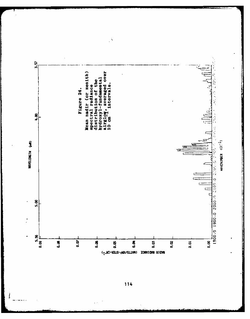
o04 00 04
N4 Vo~4
41 0 01-4) 04 OrD.,Vi
cj
114.

4-2
LI w___
?i.
-4- --
PM __ _ _ _ _ _ _ _ __ _ _ _D__ _ __ _ _ _ _ _ _ _
I- (c )
-e
cm 0TW-~S&W/iv 33 I VI

HO2 + 0 + OHt (v4 6) + 02 + 2.4 ± 0.1 eV.
It is thought to contribute principally to the dayglow (Ref 105)
at altitudes extending below those where most of the nightglow
has been found (by rocket radiometry). The two reactions
would in general result in different temporal-spatial varia-
tions of column emission, and also in a difference between
the altitude profiles of hydroxyl emission originating from
higher (v = 7,8,9) and lower (v '6) vibrational states. Both
types of effect could of course also be caused by v-dependent
collisional quenching. Some such differences have been reported
(Ref's 106, 107, 108). while other measurements have not detected
these effects (Ref's 109, 110, for example). Thus the contri-
bution of the HO2 + 0 reaction can not be considered substan-
tiated, and furthermore its principal impact would be in the
daytime when thermal emissions from the limb at OH Av = 1
wavelengths are an order of magnitude higher than at night (refer
to Fig 4). In any case, the zenith-intensity occurrence model
and spectral distribution we have derived from the data are
independent of the specific hydroxyl production mechanism.
Several attempts have been made to construct models of
the photochemistry and vertical species transport that fit
measured hydroxyl radiance variations (for example Ref's 109,
111,112, and 113). As uncertainties still exist in the radia-
tional transition probabilities, quenching rate coefficients,
and number densities of participating species (and even tempera-
ture dependence of the H + 03 reaction rate), the results of
such efforts are by and large inconclusive. Deactivation of
OHt by molecular nitrogen (cross-sections for which were most
recently reported in Ref 114) is evidenced by the cbove-mentioned
observations of energy transfer to CO2 .
van Rhijn sight-path factors for P2 - 87 + R km, l -
80 + R km are shown in Fig 6. The mean volume emission rate
per unit spectral interval or in each band would be 1/7 the
116

average zenith radiance from Fig 24 or Table 6. A nominally
more accurate limb radiance profile could be derived from
Gaussian or parabolic volume emission rate profiles (Profile
A of Ref 10 makes about the best fit to the existing set of
rocket measurements). In view of the inherent uncertainty of
the spectrum and the variability and perhaps "waviness" of the
actual profile (Section 3.5), however, the rectangular shape
is adequate for predicting the atmospheric background.
3.2. Radiance Variability
Total column emission rates in near-infrared Av - 3,
4, and 5 OH bands can be readily measured at night from ground
stations, and thus many long-period surveys of the airglow have
been made. In contrast, the altitude profile has been measured
from less than a dozen rocket probes, which have not served to
determine its systematics.
Consumption of 03 (H atoms are recycled) would pre-
dict a continuous decline in hydroxyl radiance through the
night, which is observed at low latitudes (Ref 115,116) but
much less frequently elsewhere. Models incorporating one-
dimensional transport, which advect reactants with a variable
eddy diffusion coefficient (Ref 117), have reproduced some of
the measured diurnal variations, such as the often-seen rise
in intensity after midnight at midlatitudes. Other temporal
and spatial irregularities found in the airglow -- patchiness
(Ref 118), traveling waves (Ref's 119,120), and meridional
gradients (Ref 125), for example -- may call for three- (or
perhaps two-) dimensional dynamical modeling.
Variations in the hydroxyl intensity have been found
to correlate with the occurrence of sporadic as well as re-
curring events, such as stratospheric warmings (Ref 112) and
severe magnetic storms (Ref 122). The latter (and in all
probability the former) also produce changes in the bands'
117
rotational temperature, which is in effect the kinetic temper-
ature. These episodic, propagating disturbances overlie the
more or less regular variations with mean solar ultraviolet
irradiance (which determines the altitude profiles of H and
03) and the more localized atmospheric wave-induced and
mesosphere-temperature effects.
The vast majority of existing data refer to the night-
&low. Some measurements have been made at twilight, but vir-
tually none at solar elevations above -50 because of the overlay
of Rayleigh-scattering of sunlight by the atmosphere at the
shorter hydroxyl wavelengths (which can be inexpensively
measured with uncooled spectroradiometers and are detectable
through/against the lower atmosphere, unlike the Av - 1
sequence). We have used the fact that the rates of emission
from the same upper state to two different lower states are
proportional to the Einstein coefficients for the two transi-
tions to assess the mean intensities of the fundamental bands
from the measurements of intensities in these higher overtone
sequences (Section 3.3).
In the following subsections we discuss the airglow's
variation with time of day, season of year, phase of solar
cycle, magnetic disturbance index, and stratospheric warmings.
Irregularities at a shorter spatial-temporal scale caused by
atmospheric wave phenomena are discussed separately in Section3.5. (While all but one of these column intensity variations
depend on latitude the latitude dependence of the backgroundnoise spectrums is not known.) We then develop a model of the
variation of the atmosphere's projected radiant intensity asa function of these recurring and episodic geophysical parameters,
which assumes that their effects act independently (and linearly).
This occurrence model assigns multipliers to the mean radiancewith standard deviations that estimate the uncertainty due to
the non-deterministic nature of the variability and the limi-
118
tations of existing input data. The estimated amplitudes of
infrared clutter are taken as proportional to the radiance
within the selected spectral band at the projection of the
sensor's field of view (Section 3.5).
The body of column-intensity data from ground stat-
ions allows the large-scale (-degrees of latitude) hydroxyl
surface radiances to be derived. As virtually no systematic
data exist on the smaller-scale spatial and temporal inhomo-
geneities, however, the clutter model is much less reliable
than the average-intensity model. In what follows negative
fractional uncertainties (-u), which can be comparable to 1
and thus would otherwise result in too-low (or even negative)
radiance limits, should be applied as (1 + u)-1 ; for example a
calculated total uncertainty ±70% means that the 1la range
(due to unsystematic natural behavior and/or inadequate inputinformation) would be between 1.7 and 0.59 times the quoted
best-estimate spectral radiance.
3.2.1. Diurnal Variations
Many groups (Ref's 115,122,123,124,125,126,
among others) have searched for systematically recurring
patterns in the hydroxyl nightglow, underlying (and perhaps
connected with) the fluctuations due to atmosphere dynamics.
Detailed analyses (Ref's 115,124) show that the occurrence
frequency of types of time-dependence depends on latitude and
give an indication that the distribution of these patterns
changes with season. At low latitudes a steady decrease through
the night is most commonly observed, in general agreement with
staticphotochemistry calculations. The most common diurnal
variation at midlatitude (where the most measurements have
been made) is a decrease after evening twilight to a minimum
near midnight, followed by an increase. Recurrence of nightglow
patterns gradually becomes undetectable at higher latitudes
119

(>-55*). This overall change with latitude in the diurnal
variation shows the increasing importance of species transport
at higher latitudes. We found the average ratio of highest
to lowest intensity over the course of a night to be 1.64
± 0.27, with no latitude dependence apparent within the
noise of the data set.
The most striking feature of the hydroxyl glow
near twilight is a narrow factor-about-two minimum at 4-6* solar
depression angle (Ref's 126,127,128,129). This behavior occurs
about 3/4 of the evenings (Ref 126), and also -1/4 of the
morning twilights. A measurement of the column intensity during
the day found the mean to be about the same as nightglow (Ref
129); on the other hand some calculations (Ref's 109,111)
suggest a daytime decrease by a factor as much as three.
We postpone specifying a diurnal variation model
until we have discussed the other solar zenith angle-related
changes; refer to Section 3.2.7.
3.2.2. Seasonal Variations
The distribution of time-dependence patterns
(Ref's 115,124) and the time of the nightly minimum (Ref 127)
have been reported to vary repeatably with season in the
northern hemisphere. From this variation data we have derived
a best-estimate seasonal multiplier and uncertainty:
mS = 1 + 0.26 sin [(I/3)(M - 5/2 + 2,/45)] sin i(/90 - 5/18),
us - ± 23%.
Here M is the month of the year (M - 1 refers to January) and
# is the latitude in degrees (positive in both hemispheres);
the argument of each sine function is in radians. Note that the
intensity modulation is not in phase with the mean solar eleva-
tion, but may be controlled by the mesospheric temperature (which
is a maximum in winter).
120

The average over a night of the spectral radi-
ance at month M and latitude * is found by multiplying the
mean radiance in Fig 24 or Table 6 by this factor. At * = 250
the amplitude of the seasonal modulation goes to zero, and at
700 it is a maximum of 0.26. In our model this variation is
symmetric about the equator with a six-month phase difference
between hemispheres. The la uncertainty uS (= 23%),
which is in part due to the seasonal change in occurrence of
diurnal patterns, is an average of the uncertainties in the
data sets (references above).
Stratospheric warmings, an episodic winter-
seasonal phenomenon, are discussed separately in Section 3.2.5.
3.2.3. Solar Cycle Variation
A change it, the annual-mean hydroxyl radiance
(corrected for the seasonal and diurnal variations, and again
with dynamics-induced fluctuations smoothed out) has been found
to be correlated with phase of the solar cycle at latitudes
44*N (Ref 115) and 58*N and 42*N (Ref 122). Its amplitude
averages 17%, and noise in the data set introduces an uncertainty
uC = 23%. The radiance multipler for the eleven-year solar cycle
is thus
mC = 1 + 0.17 cos [(2w/11) (Y - 1958)] ± 23%,
where Y is the year and the argument of the cosine is as usual
in radians.
This smooth variation in phase with the solar
cycle is most probably due to the increase/decrease in average
hardultraviolet energy emitted by the sun. (Solar flux varia-
tions at shorter time scales would also be expected to induce
fluctuations in the OH radiance, averaged over many days; we
have identified no direct evidence of such effects.) The
above dependence is derived from a geographically very limited
121
MA
range of observations; nonetheless as the maximum hydroxyl
emission coincides with the maximum solar flare activity,
whose effect is felt worldwide, the dependence in first approx-
imation should b2 applicable to all latitudes. The uncertainty
quoted is again an unweighted average of the uncertainties in
the individual nightglow surveys.
3.2.4. Magnetic Storm-Induced Variations
Geomagnetic storms with global magnetic index Kp
greater than about 4 have been found to produce wavelike changes
in the hydroxyl intensity (Ref 122). (The rotational tempera-
tures are also affected.) The delay of the initial enhancement
increases with decreasing latitude, while the amplitude of the
disturbance decreases. This first pulse is followed by oscill-
ations with smaller amplitudes, which extend below as well as
above the mean. Both the enhancement and its period increase
with Kp. This behavior suggests that the onset of a major
magnetic disturbance excites a wave in the mesosphere that
spreads from high latitudes (at an observed speed of 5 - 10
m/s along the meridian), decaying in amplitude. The failure
of some other surveys to detect this correlation (Ref's 124,
129) may be due to weakness of the disturbances during their
measurements, or perhaps lack of samplings when the waves
is peaking.
The maximum increase in zenith intensity resulting
from major magnetic storms is 14% per unit Kp above 4, and the
decay rate is 20% per day. An analysis of the network data in
Ref 122 indicates that the radiance multiplier at time tK in
days from the beginning of the disturbance can be expressed as
m K = 1 * G(tK, 0, Kp - 4) ± uK,
where the change due to the event is
122
iL _ _ I------

G = g cos 8 exp(-0. 2 tK),
g = 0.14 (Kp - 4) (a*2 + b* + c), and
8 = 5 (tK - 0.26 A*)/(Kp + 21).
The empirical constants are
a = 8.6 x 10 - 4 , - b - 4.0 x 10⁻², and c = 4 x 10⁻¹;
uK = ± 1.5G/mK x 100%.
This prescription holds when 4 4 Kp 4 9, * 650 . For
0 650 only an additional estimated uncertainty
uK(*> 650) = ±1.5 (0.14 (Kp - 4)] exp -(0. 2 tK) x 100%
can be applied to the radiance, as no useful data are available
on the effect of geomagnetic storms on airglow within the auroral
oval and polar cap. A* in the cyclic term is the difference
in latitude from the point of observation to the "origin" of
the disturbance, which we estimate to be at 650.
Because this origin cannot be unambiguously
determined and as no systematic data on the effect exist other
than from this one survey (Ref 122), substantial error may
result from application of the above formulas. For example,
an error in phase of the wave could even reverse the sign of
the change in hydroxyl intensity. Hence we have assigned a
large uncertainty to the enhancements excited by geomagnetic
storms.
3.2.5. Stratospheric Warming-Induced Enhancement
Similarly, the long-term effects of stratospheric
warmings (Ref 130) on the high latitude hydroxyl emission are
not well characterized. Major warmings, of scale sufficient
to cause measurable changes in the intensity (and temperature),
are thought to occur an average of once every two winters (Ref
131). They represent a meteorological effect on the mesosphere,
in contrast to geomagnetic storms, in which energy from the
thermosphere is coupled downward to the altitudes where hydroxyl
is excited.
123
An extensive survey of OH radiance during an
identified stratospheric warming was made from the OGO-4
satellite in 1967-68 (Ref 112). Emission in the (9,3) band
near 0.6225tim was found to vary with longitude (it increased
markedly above 60*N from 70*E to 70'W, for example). Increases
of up to a factor four in the nadir column intensity were re-
ported, with a factor two typical for about a month during the
late stages of the warming when the temperature wave reaches the
mesosphere. (Recall that the H + 03 reaction rate increases
with temperature.) These sole satellite data are supported by
one set of ground measurements from a station at 580 latitude
(Ref 132), from which a southward-propagating enhancement wave
with velocity 1-2 m/sec was inferred.
This thin data base does not allow prediction
of the changes in local hydroxyl radiances. The most that can
now be done is assignment of an additional uncertainty uW.
We estim&Le uW to be t 50% at latitudes above 550 and ± 30%
between 450 and 550 during major winter stratospheric warmings.
3.2.6. Latitude Effects
As we have seen, latitude comes into play in
each of these OH variations except solar-cycle. The changes
of intensity with latitude that would be due to the change in
solar ultraviolet fluence are contained in the diurnal variation
to be described below; no others can be resolved from the data
set. Latitude, then, appears as a dependent variable in the
other intensity modulations rather than as a fully independent
variable.
3.2.7. Diurnal Model
We fit the survey data on diurnal variation ofthe nightglow with equations that describe a linear decrease
after evening twilight at equatorial latitudes giving way to a
124

midnight minimum at midlatitudes, which becomes shallower toward
higher latitudes and eventually disappears into the noise. These
are the most probable patterns in each latitude region; the
less-frequent occurrence of other types of diurnal variation
is accounted for in the calculated uncertainties. The time of
day H is in hours local solar time, or Universal Time H +/- 1 hr
per 150 E/W longitude (for example at 1030 U.T. the local solar
time at 350 E is 12.83). te and tm are the local solar times
of evening and morning "hydroxyl twilight", that is, when the
local solar depression is 5* (where the minimums in the airglow
are observed). The diurnal variation multipliers for the night-
glow and their uncertainties uD are
00404260 mD - 1 - 0.04(24-H) ±33%, 24 > H ; te;
mD - 1 - 0.04H ±29%, tm > H > 0.
26(<r40* mD - 0.88 + 0.0061(H-24)2 ±10%, 24 : H > te;
mD - 0.88 + 0.0061 H2 ± 02, tm > H > 0.
40°<,(560 mD - 0.94 + 0.0033(H-24)2 ±25%, 24 > H > te;
mD = 0.94 + 0.0033 H2 ±25%, tm > H > 0;
560<04900 mD - 1 ± 63% Between OH twilights.
For the twilight and dayglow, a best-estimate
applicable to all latitudes is
mD = 0.44 + 0.56 cos [(w/12)(H-12)] ± 100%, te> Htm.
Attention is directed to the large uncertainty assigned. This
fitting function indicates a season-dependent minimum intensity
at each twilight transition, since the times at which hydroxyl-
twilight occurs vary with month of the year, and an increase
toward noon up to the mean nighttime radiance.
The local times of these twilight transitions
are determined as follows. First, the local hour angle of the
sun Hs is found from the equation
cos H. - sin(Dep)[coso cos(Dec)] - tan# tan(Dec),
where (Dec) and (Dep) are the solar declination and depression
angles. At hydroxyl twilight sin(Dep) - sin 5O - 0.087. (Dec)
125

at zonal meridians is tabulated against date in Ref 133, as is
the time of solar meridian passage ts . The local mean times
of the two twilights are:
tm i ts - Hs, te - ts + Hs,
where Hs (like H) is expressed in hours. This procedure for
finding the local times of hydroxyl twilight, which are needed
to decide whether to apply the nightglow or twilight-dayglow
formula, will be illustrated by a worked example in Section
3.4.1.
3.3. Emission Spectrum
Spectral intensities of the hydroxyl airglow measured
in Av > 1 bands -- that is, at visible and near-infrared wave-
lengths -- permit the essentially-unmeasured spectrum of the
Av = 1 sequence to be derived from ratios of intensity in
progressions (bands originating from the same upper state).
The volume rate of radiation Iij from state i to state j
is Aij ni, where Aij is the Einstein coefficient for the
transition (the inverse lifetime) and ni is the number density of
molecules in state i. Thus the rate to lower state k is simply
lk - lij x Aik/Aij.
As we noted at the start of Section 3, our occurrence model
assumes that the relative spectral distribution of OH radiation
remains constant over space and time. Consequently only the
mean radiances in single transitions originating from the
second to the ninth upper states and ratios of Einstein coef-
ficients need be known to determine the mean airglow intensity
in each fundamental vibrational band (except the (1,0), which
is determined from the population model in Ref 109).
Unfortunately, no fully coherent and reliable set of
these intensities exists. Hence we have derived a least-error
set by fitting the existing nightglow spectrum data with
measured and theoretically-derived Einstein coefficients. It
was found that the laboratory Aij's (Ref 134) resulted in
126

maximimum self-consistency of individual progression intensities
in the radiometry data base (Ref's 106,108,109,110,115,116,
117,120,125,132,135-138).
To compare the measurements from different instru-
ments and geophysical conditions, we first corrected them to
the zenith. No attempt was made to compensate for variable
attenuation by the lower atmosphere, as this effect introduces
only a small error at the long wavelengths of most of the
measurements (out-scattering is in any case largely compensated
by in-scattering from the wide-angle airglow source). We then
factored out the seasonal and solar cycle variations using the
procedure described in Sections 3.2.2 and 3.2.3. These correc-
tions reduced the average uncertainty in the combined data to
28% from its initial 70%. (The latter figure is substantiallylarger than the claimed uncertainty of individual measurements.)
We interpret this factor- 2-1/2 reduction in the spread of ab-
solute intensities of the OH IKeinel bands as evidence of the
validity of our method for removing the recurring variations
and of the accuracy of the set of Einstein coefficients adopted.
The resulting zenith intensities in the fundamental
sequence, along with the 1la uncertainty in reproducibility
of the data and the intensities calculated in Ref 99's review
of near-infrared airglow, are listed in Table 6. This distri-
bution represents a mean over the solar cycle, season, and time
of night. Fig 24's spectrum was generated with the AIRSPEC
code (Ref 50) using the Einstein coefficients in Ref 139 and
standard rotational line intensity functions (Ref 140) at a
rotational temperature of 213K, which is typical of the winter
mesosphere (Ref 141). The total spectral width of each vibra-
tional band changes by only a small amount over the range of
temperatures encountered in the mesosphere; therefore, con-
sidering also the overlap of adjoining bands and the errors
in band intensities, we have Judged a single spectrum to be
127

Specify: Mean Nadir SpectralLatitude. Longitude, Radiance x (Table 6Year, Month, Day, or Fig 24)Local Time, Kp(t);Sensor Lon itude
Generate multipliers Correct with multipliersand uncertainties for m~*,*m*X - X_ m~ - )recurring phenomena Deqeffin~ uncertainty(Sections 3.2.2, 1-2. 2 2 23.2.3, 3.2.7) U uS + N D
Kp >, Yes Gen m., x 1. X,(SeK _2. 2 2
(Se 9c 3.4) u U , + K
~K=
UK 0_
Generate van RhijnPath length multiplier,h3 CluaeSno(Fig 6 or Sec 1.4 and MVCluaeSnocos A~ cos * cos (A Long)) View Angle A~
Generate Clutter
output Spectral Radiancein detector field
±total uncertainty u.. Output Clutter
Figure 25. Flow diagram for a first-generationmodel of hydroxyl airgiow backgroundclutter.
128

adequate for the occurrence model. (Spectrums for other
temperatures can of course be readily calculated from Table 6.)
Line intensities in Fig 24 are averaged over a 10 cm "1 rectan-
gular spectrum interval.
3.4. Calculations of Column Intensity
The long-period (hours to solar cycle) temporal and
global distributions of radiance in individual bands or spectrum
intervals are calculated from the means in Table 6 or Fig 24
using the procedures described in Section 3.2. The analytic
functions that model the variations are piece-wise continuous
with latitude; discontinuities where the functions change
should be recognized as due to this quantization noise rather
than taken as a real geophysical effect, and the values faired
into one another. Similarly, the changes in intensity with year
and season, for which integer values of Y and M were derived from
the data base for input to the formulas, should be taken as
continuous.
Since the geophysical processes underlying the column
intensity changes are considered as independent of one another,
the m's can be multiplied together in any order and the total
fractional uncertainty is the square root of the sum of the
squares of the individual u's. Information on whether a major
stratospheric warming or magnetic storm is in progress, which
is available from USAF Air Weather Center as well as non-DoD
sources, is input to assess the episodic effects. Little
further error is introduced into the occurrence pattern if the
change in zenith radiance over oblique sight paths through the
emitting layer is neglected; we prescribe using the radiance
at the mid-point of the cut. Similarly, as the difference
between latitude * at the ground intercept and * at theemitting layer (shown in Fig 6) is substantial only above -55°
where the uncertainty in the airglow intensities is already
large, it can also be neglected.
129

Figure 25 is a flow chart of the procedure for calcu-
lating expectation hydroxyl background intensities and their
uncertainties. X is the mean radiance of the airgiow within
the selected wavenumber (or wavelength) interval. and the other
symbols not defined in the text are self-explanatory. As shown,the multipliers for the recurring-geophysical variations and
their uncertainties are generated to derive a provisional
x ± u', and then the magnetic storm and stratosphericwarming factors (when applicable) give the zenith radiance
x" t- u". The van Rhijn path length factor is determinedfrom the latitude and longitude of the specified sensor intercept
using Fig 6 or the equations in Section 1.4.2.1. The estimated
upper and lower limits are the expectation radiance multiplied
and divided by (1 + u )
The expected amplitude and frequency range of clutternoise superposed on this calculated average local radiance is
then derived from the simple model in Section 3.5.
3.4.1. Example Calculation
To illustrate this procedure, we work an
example for near-twilight, magnetically-disturbed conditions:
Latitude *-55 0N
Longitude =700W, sensor at 200 W.
Day/month M/year Y -01/09/1984
Time UT - 2300 U.T.
Kp - 7 storm onset 2.0 days earlier.
Seasonal: ms - 1 + 0.26 sin wr/3 (9.0 - 5/2 + 110/45) x
(Sec 3.2.2) sin w (55/90 - 5/18)
- 1.013 ± 23%.
Solar cycle: mC - 1 + 0.17 cos (2w/11) (1984 - 1958)(Sec 3.2.3) - 0.89 ±23%
130

Diurnal: Local solar time H is universal time UT
(Sec 3.2.7) corrected for the longitude difference
-70°/(15°/hr) --4.67 hr, or 23.00 - 4.67
M 18.33. We next calculate time of hydroxyl
evening twilight to determine whether to
apply the nightglow or dayglow variation
formula. Referring to Table 1 of Ref 133, we
find that at 70°W on 01 Sep local solar time
of solar meridian passage ts is 11.67 hours
and solar declination is 8.40. The hour angle
of the sun is then determined from
cos Hs = 0.087 (cos 550 cos 8.40)- 1
-tan 550 tan 8.40 = -0.0563,
Hs = 93.7 ° x 1 hr/15 0 = 6.21 hr.
Then te = ts + Hs - 11.67 + 6.21 - 17.88.
As H > te, we apply the nighttime dependence for550 latitude:
mD - 0.94 + 0.0033 (18.33 - 24) 2 25%= 1.05 ± 25%
Recurring: m' = mS • mC. mD = 0.95u- = (0.232 + 0.232 + 0.252)1/2 = ± 41%.
Magnetic Storm: mK - 1 + 0.14 (7 - 4) [8.6 x 10- 4 (55)2
(Sec 3.2.4) - 0.040 (55) + 0.4] x
cos 5[(2 - 0.26(65 - 55))/28]exp(-0.4)-1.11
uK - (1.5) (0.11)/1.11 - ± 13%.
Stratwarm: M * 12, 1, 2, or 3; therefore no change.
(Sec 3.2.5)
Total m "' - m* mK - 1.05
Zenith: u - (0.412 + 0.132 + 02)1/2 = ± 43%
131

Pathlength: Referring to Section 1.4.2.1, the angle
between the exoatmospheric measurement platform
nadir and the point of observation is found
from
cos x - cos 0 cos (A longitude)
= cos 550 cos (700-200) = 0.3687,
= 68.370.
The elevation angle of the sight path is found from
sin o = sin A/(P/R - cos 0)
= 0.9300/(6.6321 - 0.3667) = 0.1485,
0 = 8-540.
As this angle intercepts the earth's surface
(see Fig 6), the path length for o2 = 87 km + R,
Pl = 80 km + R is given by the first of the
formulas in Sec 1.4.2.1. Substituting P2,
Pl, P = 6.6321 R, R = 6370 km, and sin 2 0,
we find the pathlength is 30 km.
Therefore mv = 30/7 = 4.3.
Radiance m-1 = m- . mv - (1.05) (4.3) = 4.52 . 43%.
Multiplier:
Thus the projected sky radiance in, for example, the total
(13 w/km 2 ster) hydroxyl band system would be k .
59 + 25, - 18 w/km 2 ster.
3.5. Clutter Statistics
Irregular, non-systematic variations also appear in
the hydroxyl nightlow. These have at least two loosely-defined
spatial-temporal scales, -5 min-25 km horizontally and -3 hr-
thousands km. The latter modulations, whose occurrence statis-
tics is poorly understood (largely because their scale is close
132

have amplitudes of about 10% and are considered to be associated
with traveling ionosphere disturbances (Ref 142). The shorter-
wavelength irregularities are thought to be due to internal
gravity waves (Ref 143,144) that have their origin In disturb-
ances of either the troposphere (principally) or thermosphere.
As their scale is much closer to that of the footprints and
signal integration times of typical measurements sensors, they
would be the major source of clutter from hydroxyl.
3.5.1. Zenith Data
No quantitative data exist on the frequency
spectrum of this background in near-limb projections. The
measurements from below the layer have focused principally on
temporal variations, with some preliminary spatial cross-
correlations determined using a multiple-field Av = 4-bands
photometer (Ref 145). Spatial scans of Av = 1 and 2 emission
made with AFGL's optical aircraft flying at 220 m/sec (Ref 31)
and with a radiometer whose field of view was rotated in a
vertical plane at 21 elevation/sec (Ref 146) (a horizontal
sweep speed of 3 km/sec at the zenith) do not differ qualita-
tively from the many temporal scans made with fixed-pointing
instruments. (These hydroxyl data bases are available for
quantifying the short-period spatial variations.)
Narrow-field groundbased instruments -- with
footprint <5 km on the hydroxyl layer -- show the variation to
have amplitude 2-3% in a band of frequencies near 1/5 min- I
(Ref's 142, 143, 145, for example). No power spectral densities
have been reported in the journal literature, presumably be-
cause this fluctuation signal is so weak. Reports of arge
episodic changes -- "spikes" or "ledges" of scale less than a
few min and amplitude greater than a few percent, not due to
cloud or instrument effects -- are conspicuously missing from
the literature.
133Li
- .. WhOW.A.&

LU
2->
LU
Q) 4-
.c2 0
00 0)>-
4 Q)4-4 ~.)
I-4 Cd - l
'-E -~) bt 4-
Q) C, ~) Wz4-)X 0W
00) 4-) 4-)
0 O"o
0 ,- .4) 4-)
> 0ogob~)C11 b
2) 4-4 ) I
- C.) 'W4-.H 2 S.
134
1 I
How the rms amplitude or the frequency range
of this irregularity depends on average airglow radiance,
latitude, or other geophysical parameters, is not known. One
model (Ref 149) suggests that at least one type of short-
period irregularity is excited when longer-period atmospheric
waves reach a threshold amplitude. While the disturbances
might be expected to be more intense and frequent at high
latitudes (Ref's 3,148), especially in the winter mesosphere
(Ref 142), the direct evidence is not useful for modeling such
behavior. We have not attempted to extract this information
from the nightglow data base, as instrument noise and data
smoothing (seldom specified) would most probably mask any
systematic changes.
3.5.2. Low Elevation-Angle Data
Spatial distributions of OH radiance near
the horizon can be measured by conventional photography from
mountain or aircraft altitudes (Ref 107). The van Rhijn gain
raises the irradiance in the image plane over the effective-
exposure threshold of near Infrared-sensitive emulsions (Ref
142), and simultaneously an enhancement of the projected ir-
regularity results in readily-detectable contrast on the
negative (rather than a smooth and thus virtually uninterpre-
table density distribution). At zenith angles greater than
about 700 -- an angle of 220 between line of sight and
hydroxyl layer -- the amplitude of the spatial variations in
the Av = 4 and 5 bands within the camera's spectral range
increases to about 15% in many of the photographs (Ref 150).
The low-to-the-horizon nightglow shows as a series of more or
less regularly rippled clouds separated by a few 10's of km
and traveling perpendicular to their length in a horizontal
plane, and sometimes as patches whose spatial frequency
spectrum would be isotropic. No favored direction of the
135

waves has been identified. Occurrence of this structure Is
reported by one group to be correlated with lunar high tide
'Ref 148), which they interpret as due to excitation of second-
ary shorter waves in the mesosphere by a harmonic of the lunar
atmospheric tidal wave. The literature does not provide quan-
titatIve information on the probabilities of occurrence of
amplitude of this radiance modulation.
Other investigators (Ref 150, 151) explain the
measurei sky brightness distributions by invoking a "corrugated"
emitting layer whose vertical amplitude/horizontal wavelength
ratio Is -1/20, such as is shown in Figure 26. Near the
zenIlth, the line of sight intercepts the layer once; variations
in ra~idance are due to the small changes in pathlength as Its
ank, to th layer Thanges. Near the horizon (sight paths
A,P,C), the nolulation of the pathlength gain factor would
increase rapidly, with multiple intercepts on the waves at low
Incidenoe angles. (Near-horizon views also enhance the relative
sIght path through the bottom edge of tne emitting volume,
where most of the irregularity is expected (Ref" 148)). This
height variation implies that the maxim~n, van RhiJn factor for
hydroxyl (in Section 1.4) is somewhat overestimated.
Tnis airglow geometry indicates that the peaks
should appear closer together as F decreases. That this
foreshortening toward smaller spatial-scale Irregularities has
not been reported for & between 220 and 9-1/2' (0' eleva-
tion, about the limit of view on the photographic images) is
most probably due to the nonuniformity of the wavelength.
From the near-zenith temporal (and spatial) variations anj
gravity wave theory, it may be concluded that a broad band of
spatial frequencies is present in the emitting layer, which
would have the effect of attenuating higher-frequency structure
at low incidence angles (such as those of limb views from
rockets or satellites).
136

3.5.3. Clutter Amplitude and Frequency
This incidence angle F Is the key variable in
modeling the short-period, short-wavelength hydroxyl radiance
v~riatlon seen from space. From geosynchronous orbit reaches
220 at an elevation angle o of 8.140 (refer to Fig 6); there-
fore the ground-intercept latitude in the nadir meridian (or the
spherical angle x from the earth's center) is 59.80. The
groundbased hydroxyl-radiometry data Indicate that when
o 4 8.140, where the points on the earth's surface are at
X 59.80 and the van Rhijn gain is thus 42-1/2, the rms
amplitude of this clutter Is
0.02 x average radiance X-, with 70% probability
0.03 x average radiance, with 30% probability.
For the range 22' >c) 9.30,
which corresponds to 8.14' 4o4 8.68' and
59.80 <X- 81.32',
we take the fluctuation amplitude to be larger and again
proportional to the average radiance. We deduce from the
available data that weak disturbances resulting from the
layer having the shape indicated in Fig 26 are always present,
and are overlaid roughly half the time by a strong disturbance
(perhaps resulting from the nonlinear lunar-tide process de-
scribed in Ref 148) with the microdensitometrically-measured
amplitude reported in Ref 150. Some probability of even
larger excursions is included to err on the side of conserva-
tism. The estimated fluctuation amplitudes are then
0.07 x average radiance, with 50% probability
0.15 x average radiance, with 40% probability
0.20 x average radiance, with 10% probability.
These occurrence probabilities are to be taken as independent
of the direction in the horizontal plane in which the measure-
ments sensor is pointing, latitude, mean radiance, and solar
time. (A variation with time of lunar transit would be included
137
when the data of Ref 148 are refined.) Note that when x
81.320 the sensor's sight path is tangent to the earth's
surface, which is the effective limit of the photographic
measurements of hydroxyl emission structure.
For the range of o over which the geo-
synchronous sensor's field of view intercepts the hydroxyl
layer but not the earth, which is
6.680< < 8.820
which corresponds to 9.3' > - O ,
no structure data from the bottomside are available. Ref 150's
geometric model does not show 9.30 to have any special property,
and the presence of a distribution spectrum of wavelengths
indicates no change in the spectrum of radiance variations at
these low incidence angles. Hence we prescribe continuing the
probability distribution of clutter amplitudes for & 220 to9.30 down to 0*.
These background radiance variations extend
over spatial frequencies 1/50 km- 1 to 1/10 km-1 in the photo-
graphic data. The qualitative similarity between temporal
and spatial scans of the radiation, supported by the theory of
these fluctuations (Ref's 143, 152), suggests that the same
frequencies are present when 4 >220. The best-estimate of the
spatial power spectral density of hydroxyl noise seen by a geo-
synchronous experiment sensor is thus
(0.03 or 0.02 radiance)2
per cycle/km, o <6.14 0 , x <59.80
(0.20, 0.15 or 0.07 radiance)2
per cycle/km, 0 #8.140, X >59.80.The same prescription applies to the temporal PSD's in the
frequency band between 1/600 and 1/100 Hertz. No reliable
estimate can be made of probabilities of exceedance of spectral
138

power beyond those derivable from the estimated occurrence
probabilities.
At the current state of knowledge, these
estimates of the clutter background can be taken as applicable
to all projected hydroxyl radiances under all geophysical
conditions.
3.6. Hydroxyl Data Base
It is clear that the existing information on hydroxyl-
emission irregularities, in particular those in limb views of
the layer, is sufficient to construct only a rudimentary model
of the infrared clutter background. The spatial and temporal
noise spectrzns at incidence angles as low as 6.770(0 = 8.730)
could be determined by measurements from balloon altitudes.
The short-wavelength irregularities' frequency spectrum, with
its occurrence statistics and dependence on geophysical para-
meters, could be derived from ground and aircraft measurements;
indeed, some unanalyzed existing data contain this type of
information. Surveys of the airglow's radiance structure from
satellite and even sounding rockets would of course provide the
most directly-applicable inputs to design of future measurements
experiments, as is the case for the auroral infrared backgrounds.
This review has also shown broad gaps in the data on
other important aspects of the hydroxyl vibrational-bands back-
ground. Information is lacking on, for example, the basic
radiative and collisional deactivation parameters of OHt; the
systematics of airglow intensity averaged over -1 hr through
the day; and in the spectral distribution in the fundamental
sequence, particularly in above-the-limb projections.
139
" I *
REFERENCES
1. T.C. Degges and H.J.P. Smith, A High Altitude InfraredRadiance Model, AFGL-TR-77-0271 (30 Nov 77).
2. F.Y. Kneizys, E.P. Shettle, W.O. Gallery, J.H. Chetwynd, Jr.,L.W. Abreu, J.E.A. Selby, R.W. Fenn, and R.A. McClatchey,Atmospheric Transmittance/Radiance: Computer Code LOWTRAN 5,AFGL-TR-80-0067 (21 Feb 80).
3. J.E.A. Selby, F.X. Kneizys, J.H. Chetwynd, Jr., and R.A.McClatchey, Atmospheric Transmittance/Radiance: ComputerCode LOWTRAN 4, AFGL-TR-78-0253 (1978).
4. C.H. Humphrey, R.M. Nadile, C.R. Philbrick, and D.R. Smith,Atmospheric Infrared Radiance Variability, AFGL-TR-81-0207 (27 May 81).
5. I.L. Kofsky and J.W. Schroeder, Visible and InfraredRadiations from the atmosphere Accompanying PCA Events,AFCRL-TR-74-0476 (30 Sept 74).
6. R.R. O'Neil, A.T. Stair, Jr., E.T.P. Lee, D. Burt, andG. Frodsham, Excede Spectral: An Artificial AuroralExperiment, Paper 81-0422, AIAA 19th Aerospace SciencesMeeting, St. Louis, 1981.
7. K.D. Baker, D.J. Baker, J.C. Ulwick, and A.T. Stair, Jr.,Rocketborne Measurement of an Infrared EnhancementAssociated with a Bright Auroral Breakup, AFGL-TR-77-0157 (05 Jul 77).
8. S.-I. Akasofu, Polar and Magnetospheric Substorms,Springer, New York, 1968.
9. C.M. Langley and W.G.M. Blaettner, E-O Sensor SignalRecognition: Computer Code SPOT I, Radiation ResearchAssociates (Ft. Worth, TX) Report T7809 (01 Oct 78).
10. W.F. Grieder and L.A. Whalen, Geometric Aspects ofRocket Photometry, AFGL-TR-76-0046 (Feb 76).
11. J.W. Chamberlain, Physics of the Aurora and Airglow,
Academic Press, New York, 1961.
12. D.W. Swift, Rev's Geophys. Space Phys. 17, 681 (1979).
13. Y.I. Feldstein and G.V. Starkov, Planet. Space Sci.15, 209 (1967).
140

REFERENCES (continued)
14. J.A. Whalen, General Characteristics of the AuroralIonosphere, in Physics of Space Plasmas (ed's T. Chang,B. Coppi, and J. Jasperse), SPI Conference and ReprintSeries 4, Scientific Publications, Cambridge, MA (1981).
15. C.P. Pike and J.A. Whalen, J. Geophys. Res. 79, 985 (1975).
16. A.T.Y. Lui and C.D. Anger, Planet. Space Sci. 21, 799 (1973).
17. G. Davidson, The Use of Digital DMSP Data for AuroralMeasurements, AFGL-TR-81-0105 (15 Feb 81).
18. J.B. Kumer, R.D. Sears, J.E. Evans, S.E. Harris, and R.M.Nadile, Application of Visible Monochromatic AuroralImaging Data for Modeling Infrared Earth-Limb Morphology,AFGL-TR-81-0025 (26 Mar 81).
19. A. Omholt, The Optical Aurora, Springer, New York, 1971,Chapter 7.
20. G.G. Shepherd and E.V. Pemberton, Radio Sci. 3, 650 (1968).
21. A.P. Krukonis and J.A. Whalen, J. Geophys. Res. 85, 119(1980).
22. R.E. Sheehan, R.L. Carovillano, and M.S. Gussenhoven,J. Geophys. Res. 87, 3581 (1982).
23. R.A. Hoffman and J.L. Burch, J. Geophys. Res. 78, 2867(1973).
24. P.J. Tanskanen, D.A. hardy, and W.J. Burke, J. Geophys.Res. 86, 1379 (1981).
25. D.J. Strickland, Electron Transport, Chemistry, andOptical Emissions in the Auroral E-Layer, AFGL-TR-81-0042(Jan 81).
26. M.H. Rees and D. Luckey, J. Geophys. Res. 79, 5181 (1974).
27. I.L. Kofsky, Ultraviolet-Optical Remote Sensing of theIonosphere, AFGL-TR-77-0142 (30 Jun 77).
28. R.L. Arnoldy and P.B. Lewis, Jr., J. Geophys. Res. 82,5563 (1977).
29. L.A. Frank and K.L. Ackerson, J. Geophys. Res. 76, 3612(1971).
141

REFERENCES (continued)
30. R.K. White, Incoherent Scatter Radar Measurements in theUpper Atmosphere, DNA 3082T (Nov 77).
31. I.L. Kofsky, D.P. Villanucci, and R.B. Sluder, Evaluationof Infrared Simulation Data, DNA 5521F (26 Nov 80).
32. S.B. Mende and R.H. Eather, J. Geophys. Res. 80, 3211(1975).
33. I.L. Kofsky, J.D. Geller, and C.A. Trowbridge, Sky Back-ground Measurement Program, AFCRL-70-0032 (30 Nov 69).
34. R.H. Eather and S.B. Mende, J. Geophys. Res. 76, 1976(1971).
35. A. Belon, G. Romick, and M.H. Rees, Planet. Space Sci.14, 597 (1966).
36. L.G. Jacchia, Smithsonian Astrophysical Report 375,Cambridge, MA (1977).
37. C.S. Deehr, J.D. Winningham F. Yasuhara, and S.-I. Akasofu,J. Geophys. Res. 81, 5327 (1976).
38. T.L. Stephens (Kaman TEMPO), Private communication (1982).
39. D.H. Archer, Infrared Program Support, Final Report onDNA-001-81-0011, DNA-0000 (30 Nov 81).
40. D.J. Baker, G.D. Frodsham, J. Kumer, A.T. Stair, Jr.,and J.C. Ulwick, Trans. Am. Geophys. Un. 60, 328 (1979).
41. I.L. Kofsky, D.P. Villanucci, and W.S. Andrus, Assessmentof Rocketborne and Airborne Infrared Data, DNA 4731F(30 Nov 78).
42. I.L. Kofsky, D.P. Villanucci, and G. Davidson, Assessmentand Evaluation of Simulation Data, DNA 4303F (15 Nov 77).
43. D.H. Archer, Requirements for Im proved Infrared PredictionCapability, DNA 4585F (30 Apr 78).
44. G.E. Caledonia and J.P. Kennealy, NO Infrared Radiationin the Upper Atmosphere, submitted to Planetary and SpaceScience (1982).
45. W.P. Reidy, T.C. Degges, A.G. Hurd, A.T. Stair, Jr., andJ.C. Ulwick, J. Geophys. Res. 87, 3591 (1982).
46. W.T. Rawlins, G.E. Caledonia, J.J. Gibson and A.T.Stair, Jr., J. Geophys. Res. 86, 1313 (191).
142
• . . .. . . f ' .. . .. . . . .. ... .. . .. .... - -''t ~ J I . . .g; . , , - . .. . ... . . . . -.

REFERENCES (continued)
47. J.P. Kennealy, F.P. Del Greco, G.E. Caledonia, and B.D.Green, J. Chem. Phys. 69, 1574 (1978).
48. F.P. Billingsley II, J. Molec. Spectrosc. 61, 53 (1976).
49. I.L. Kofsky, D.P. Villanucci, and R.B. Sluder, DataReduction and Auroral Characterizations for ICECAP III,DNA 4220F (31 Jan 77).
50. I.L. Kofsky, C.A. Trowbridge, and R.B. Sluder, DataReduction and Auroral Characterizations for ICECAP 11,DNA 3789F (25 Oct 75).
51. I.L. Kofsky, D.P. Villanucci, M.T. Chamberlain, and C.A.Trowbridge, Further Evaluations of Infrared SimulationData, DNA-TR-81-41 (30 Nov 81).
52. D.H. Archer (Mission Research Corp.), Private communica-tion (Mar 82).
53. J.P. Heppner and M.L. Miller, J. Geophys. Res. 87, 1633(1982).
54. R.E. Good and C.A. Trowbridge (AFGL), Private communica-tion (1982).
55. G.D. Nastrom, B.B. Balsley, and D.A. Carter, Geophys.Res. Lett. 9, 139 (1982).
56. R.G. Roble, R.E. Dickinson, and E.C. Ridley, J. Geophys.
Res. 87, 1599 (1982),
57. G.V. Groves, J. Brit. Interplan. Soc. 22, 285 (1969).
58. U.S. Standard Atmosphere, NOAA-S/T 76-1562 (1976).
59. J.-C. Gerard and C.A. Barth, J. Geophys. Res. 82, 1674(1977).
60. J.B. Kumer, Analysis of 4.3on ICECAP Data, AFCRL-TR-74-0334 (Jul 74).
61. J.B. Kumer and T.C. James, J. Geophys. Res. 79, 638(1974).
62. J.B. Kumer, J. Geophys. Res. 82, 2203 (1977).
63. J.B. Kumer, Multidimensional Time Dependent Structureand Mechanisms for Non-LTE CO2 Infrared Emissions and4.3m Aurora, AFGL-TR-79-0224 (31 Aug 79).
143

REFERENCES (continued)
64. D. Garvin and R.F. Hampson, Chemical Kinetics Data SurveyVol 7, National Bureau of Standards TR1974-30 (1974).
65. H. Trinks and K.H. Fricke, J. Geophys. Res. 83, 3883(1978).
66. D. Offermann and K.U. Grossmann, J. Geophys. Res. 78, 8296(1973).
67. D.J. Baker, G.D. Frodsham. J. Kumer, A.T. Stair, Jr., andJ.C. Ulwick, in Proceedings of the Second DNA InfraredData Review Meeting (ed's A.T. Stair, Jr., and J.A. Mayo),AFGL-TM-18 (1979).
68. E.T.P. Lee, R.R. O'Neil, and A.T. Stair Jr., in EXCEDESpectral Preliminary Results (ed. R.O.'Neil), AFGL-TM-41(1980).
69. F. Bien, Measurements of Nitric Oxide Vibrational Absorp-tion Coefficient and Vibrational Transfer to N2 , AFGL-TR-77-0181 (Sep 77).
70. R.H. Eather, Rev's Geophys. Space Phys. 11, 155 (1973).
71. A.T.Y. Lui, C.D. Anger, D. Venketesan, W. Sawchuk, andS.-I. Akasofu, J. Geophys. Res. 80, 1795(1975).
72. R.E. Sheehan, M.S. Gussenhoven. and R.L. Carovillano,Activity Rating Scheme and Latitudinal Extent ofDMSP Auroras, Boston College Report BC-76 801 (1976).
73. G. Gustafsson, Latitude and Local Time Dependence ofPrecipitated Low Energy Electrons at High Latitudes,NASA X-645-72-293 (Aug 72).
74. G. Rostoker, Rev's Geophys. Space Phys. 10, 935 (1972).
75. S.L. Valley (ed.), Handbook of Geophysics and SpaceEnvironments, McGraw-Hill, New York. 1965, Section 11.
76. A.V. Jones, Aurora, Reidel, Dordrecht, 1974.
77. B.S. Dandekar, Study of Equatorward Edge of the Auroral
Oval from Satellite Observations, AFGL-TR-79-0010 (09 Jan 79).
78. G.V. Starkov, Geomag. i Aeron. 9, 614 (1969).
79. R.E. Sheehan and R.L. Carovillano, J. Geophys. Res.
83, 4749 (1978).
144

REFERENCES (continued)
80. B.S. Dandekar, AFGL Report TM-86, in preparation (1982).
81. B.S. Dandekar, Magnetic Disturbance Statistics from aSingle Station Q Index Applied to an Actual OTH-B RadarStation, AFGL-TR-79-0296 (18 Dec 79).
82. A.E. Reilly, The Geomagnetic Index Q -- Its Persistence,Predictability, and Other Pertinent Properties,AFGL-TR-78-0223 (18 Sep 78).
83. A.L. Cage and E. Gawalick, A Discussion of GeomagneticIndices Kp and Ap, 1932-1971, AFCRL-72-0693 (Nov 72).
84. R.H. Holzworth and C.-I. Meng, Geophys. Res. Lett. 2,377 (1975).
85. J.A. Whalen, Auroral Oval Plotter and Nomograph forDetermining Corrected and Geomagnetic Local Time,Latitude, and Longitudes for High Latitudes in theNorthern Hemisphere, AFCRL-70-0422 (27 Jul 70).
86. J.E. Evans, L.L. Newkirk, and B.M. McCormac, NorthPolar, South Polar, World Maps and Tables of InvariantMagnetic Coordinates for Six Altitudes, DASA 2347 (Oct 69).
87. J.A. Whalen (AFGL), Private communication (1982).
88. U.S. Naval Observatory Air Almanac, Washington, 1982.
89. B. Hultqvist and G. Gustafsson, J. Atm. Terr. Phys.19, 246 (1960).
90. R.L. Carovillano, G.L. Siscoe, R.E. Sheehan, R.H. Eather,M.S. Gussenhoven, and N.U. Crooker, Unified Model ofAuroral Substorm Development, AFCRL-TR-75-0558 (31 Aug 75).
91. R.H.Eather, J. Geophys. Res. 84, 4134 (1979).
92. J.E. Maggs and T.N. Davis, Planet. Space Sci. 16,205 (1968).
93. Y. Kamide and J.D. Winningham, J. Geophys. Res. 82,5573 (1977).
94. T.R. Hartz, Particle Precipitation Patterns, in TheRadiating Atmosphere (ed. B. McCormac), Reidel,Dordrecht, 1971.
95. G. Davidson and C.A. Trowbridge (PhotoMetrics, Inc.),Private communication (1982).
145
REFERENCES (continued)
96. R. Sears, Experimental Visible Spatial Structure, inProceedings of the Second DNA Infrared Data Review Meeting(ed's A. T. Stair, Jr. and J. A. Mayo), AFGL-TM-18(1979).
97. A.B. Meinel. Astrophys. J. 111, 555 (1950).
98. J.B. Kumer, A.T. Stair, Jr., N. Wheeler, K.D. Baker andD.J. Baker, J. Geophys. Res. 83, 4743 (1978).
99. A. Vallance Jones, Space Sci. Rev's 15, 355 (1973).
100. D.R. Bates and M. Nicolet, J. Geophys. Res. 55, 301 (1950).
101. G. Herzherg, J. Roy. Astron. Soc. Can. 45, 100 (1951).
102. D.L. Baulch. R.A. Cox, R.F. Hampson, Jr., J.A. Kerr,J. Troe, and R.T. Watson, J. Phys. Chem. Ref. Data 9,295 (1980).
103. M. Nicolet. Planet. Space Sci. 20, 1671 (1972).
104. M. Nicolet, Ann. Geophys. 26, 531 (1970).
105. E.L. Breig. Planet. Space Sci. 18, 1271 (1970).
106. H. Takahashi and P.P. Batista, J. Geophys. Res. 86. 5632(1981).
107. V.I. Krassovsky and M.V. Shagaev, Planet. Space Sci. 25,509 (1977).
108. J.W. Rogers. R.E. Murphy, A.T. Stair, Jr.. and J.C. Ulwick.J. Geophys. Res. 78, 7023 (1973).
109. E.J. Llewellyn. B.H. Long, and B.H. Solheim, Planet. SpaceSci. 27, 1421 (1979).
110. L.M. Kieffaber and A.W. Peterson, J. Atmos. Terr. Phys.40. 1339 (1978).
111. E. Battener and J.J. Lopez-Moreno, Planet. Space Sci. 27,1421 (1979).
112. J.D. Walker and E.I. Reed, Behavior of the Sodium and Hy-droxyl Nighttime Emissions During a Stratospheric Warming,NASA/Goddard Space Flight Center Report X-621-76-6 (1975).
113. G. Moreels, G. Megie, A. Vallance Jones, and R.L. Gattinger,J. Atmos. Terr. Phys. 39, 551 (1977).
114. G.E. Streit and H.S. Johnston, J. Chem. Phys. 64, 95 (1976).
146

REFERENCES (continued)
115. R.H. Wiens and G. Weill, Planet. Space Sci. 21, 1011 (1973).
116. G. Fiocco and G. Visconti, J. Atmos. Terr. Phys. 36, 583(1974).
117. G. Moreels, D. Chahrokhi and J.E. Blamont, J. Geophys.
Res. 81, 5467 (1976).
118. A.W. Peterson and L.M. Kieffaber, Nature 242, 321 (1973).
119. J.F. Noxon, Geophys. Res. Lett. 5, 25 (1978).
120. B.R. Clemesha, V.W.J.H. Kirchoff, D.M. Simonich, H. Taka-hashi, and P.P. Batista, J. Geophys. Res. 84, 6477 (1979).
121. F.A Herrero and J.W. Meriwether, Jr., J. Geophys. Res.85, 4191 (1980).
122. N.N. Shefov, Planet. Space Sci. 17, 797 (1969).
123. P. Berthier, Ann. Geophys. 12, 113 (1956).
124. M. Nakamura, Symposium on the Ionospheric Regions: Proc.Inst. Space Aero. Sci., University of Tokyo, 153 (1974).
125. F.E. Bunn and H.P. Gush, Can. J. Phys. 50, 213 (1972).
126. R.J. Huppi and D.J. Baker, Intensity Variations of Atmos-pheric Hydroxyl Emissions, AFGL-TR-76-0032 (1976).
127. K.A. Dick, Ann. Geophys. 28, 149 (1972).
128. D.R. Pick, E.J. Llewellyn, and A. Vallance Jones, Can. J.Phys. 49, 897 (1971).
129. G. Moreels, W.F.J. Evans, J.E. Blamont, and A. VallanceJones, Planet. Space Sci. 18, 637 (1970).
130. K. Labitzke, J. Atmos. Sci. 29, 1395 (1972).
131. M.R. Schoeberl, Rev's Geophys. Space Phys. 16, 521 (1978).
132. N.N. Shefov, Ann. Geophys. 28, 137 (1972).
133. B.P. Sandford and L.R. Doan, Graphs of the Solar Depres-sion Angle from 0* to 900, AFCRL-69-0543 (1969).
134. R.E. Murphy, J. Chem. Phys. 54, 4852 (1971).
147

REFERENCES (concluded)
135. R.E. Goody, Planet. Space Sci. 24, 389 (1976).
136. T. Watanabe, M. Nakamura, and T. Ogawa, J. Geophys. Res.
86, 5768 (1981).
137. V.I. Krassovsky, Ann. Geophys. 28, 739 (1972).
138. R.G. MacDonald, H.L. Buijs, and H.P. Gush, Can. J. Phys.46, 2575 (1968).
139. F.H. Mies, J. Molec. Spectrosc. 53, 150 (1971).
140. G. Herzberg, Spectra of Diatomic Molecules, Van NostrandReinhold, New York, 1950.
141. Cospar International Reference Atmosphere, Akademie-Verlag, Berlin, 1972.
142. I.L. Kofsky, J.W. Meriwether, Jr., J.W. Schroeder, andR.B. Sluder, Data Reduction and Auroral Characteriza-tions for ICECAP, DNA 3511F (10 Apr 75).
143. R. Hatfield, T.F. Tuan and S.M. Silverman, J. Geophys.Res. 86, 2429 (1981).
144. T.F. Tuan, Research in Gravity Waves and Airglow Pheno-mena, AFGL-TR-76-0296 (1976).
145. R.D. Sears, Ground-Based Photometric Measurements, DNA4975 (31 Jan 79).
146. Ground Support Data Report in Support of Black Brant18.219-1 Flight, Utah State University (02 Sept 74).
147. T. Sugiyama, Ionosphere Symposium of the University ofTokyo (Oct 75).
148. A.W. Peterson, L. Kieffaber, T.F. Tuan, D. Papadopoulos,and R.M. Nadile, submitted to J. Geophys. Res. (1982).
149. M. Davis and A.V. DaRosa, J. Geophys. Res. 74, 5721 (1969).
150. M. Herse, G. Moreels, and J. Clairemidi, Appl. Opt. 19,355 (1980).
151. G. Moreels and M. Herse, Planet. Space Sci. 25, 265 (1977).
152. T.F. Tuan, Theoretical Investigation of the Effects of At-mospheric Gravity Waves on the Hydroxyl Emissions of theAtmosphere, AFGL-TR-80-0007 (1979).
153. L. H. Keiffaber and A. W. Peterson, J. Atm. Terr. Phys. 40,
1339 (1978).
148
kI
APPENDIX I
NITRIC OXIDE VIBRATIONAL-OVERTONE AIRGLOW
BACKGROUND
The major source of excitation of NO (v>2) in the mid-
latitude (non-auroral) daytime upper atmosphere is the reactions
of ambient 02 with N atoms that result from dissociation of
N2 molecules by solar photons and their secondary electrons.
At night [N] decreases by about two orders of magnitude in the
altitude range where these reactions produce significant dayglow
(aeronomy model results, Ref I-i), reducing +d[NOt ]/dt by the
same factor.
Other processes that could excite NO (v>2) in the thermo-
sphere occur either less frequently or are unverified. The quench-
ing reaction N2 (A) + 0, even if it always produces NO t (which has
not been observed experimentally), would result in a lower
volume excitation rate at most altitudes. (The concentration of
N2 (A) in the atmosphere above - 120 km can be estimated
from the intensity of dayglow in the Vegard-Kaplan (A-X) bands.)
N(4 S) + 02( 1A) is similarly both infrequent and with uncertain
yield of NOt. The column emission rates of solar-pumped electronic
bands of NO (8,-y, 6) are so low that the ensuing vibrational
cascade is only of the order of 10-2 as intense as chemilumin-
escence. Thermal population of NO to the Av = 2 state is also
small compared to daytime N + 02, as current atmospheric limb
emission models show (Ref 1-2); however, when [N] decreases at
night it is about the same order of magnitude. Scattering of
solar photons from NO, H20, and CO2 molecules also produces less
volume emission in cne 2.7pm region above -110 km altitude,
according to limb models (Ref 1-2).
This chemiluminous dayglow was in fact considered in the
initial treatments of upper-atmospheric NOt-production processes,
149
Ref's 1-3 and 1-4. At the time no measurements were available
of [N] or of yields of NOt from the reaction of ground-state
and excited N atoms with 02 (since measured by AFGL). (Ref 1-3
presents calculated fractional rates of vibrational excitation
of ambient NO molecules, rather than sky background radiances
in the overtone band.)
INTENSITY CALCULATIONS
We have calculated The zenith and limb brightnesses in the NO
overtone sequence using the midwinter 1400 LT profiles of [N4S]
and [N2 D + 2pI from Ref 1-5, and the [02] and temperature profiles
from the Jacchia 1977 Atmosphere (Ref 1-6; about exosphere tempera-
ture about 1020 K). The yield of overtone photons was taken as
1/3 in each reaction of the metastable N atoms with 02 (calcu-
lated from 0.7% auroral chemiluminous efficiency for NO overtone
radiation, with 1-1/2 N2 D + N2 p atoms produced per ion
pair) and 1/4 in the reactions of ground-state N (which are less
exothermic and thus result in less vibrational excitation).
The zenith radiance in the nitric oxide overtone is then
the sum over altitude
LiO 2 (1/4[N SI 3 x 10- 2exp(-3150/T) + 1/3[N2D + 2P] 5.2 x 10⁻¹²),
where the numerical figures just after the atomic nitrogen
concentrations are the rate coefficients for reaction of each
species with 02 to produce NO, and T is the ambient kinetic
temperature at the altitude considered.
The results are as follows. Little radiation is emitted
below 100 km because the natural N-atom concentrations are decreas-
ing rapidly near that altitude. The volume emission rate profile
then shows an increase to a flat maximum (near 2000 photons/cm 3 sec
over - 40 km) near 160 km. 2/3 of the emission is due to the
N2 D + 02 reaction. (Using a rate coefficient of only 2.7 x 10⁻¹ 2
cm 3/sec for the N2 D + 02 reaction and earlier altitude
profiles of [N], another group (Ref 1-7) has calculated that 1/5
of the NO production, and thus -1/4 of the overtone emission,
150

is due to the metastable-state reaction.) The total daytime
vertical-column radiance is 1 watt/km 2 ster. Maximum bright-
ness in the limb for the broad layer is then about 30 w/km 2-
ster, which is near the 10 w/km 2-ster minimum stated in Section
1.2. (All figures are accurate to only a factor -2 because
of uncertainties in the input concentration profiles.)
By night the predicted precipitous drop in [N] (Ref I-i)
reduces the calculated radiances in the NO overtone by about two
orders of magnitude below these daytime figures. Some recent
rocket profiles at 31'N latitude (Ref 1-8) indicate signifi-
cantly higher nighttime vertical column intensities near 2.6 n;
however, as these radiometer data would result in factor-100
higher nightglow radiances in the N2 D-4S airglow doublet
at 0.5200im than are observed, and in addition fail to show
the accepted hydroxyl-fundamental profile, they are subject to
question. (None of AFGL's rocket probe data apply unambiguously
to measuring the NO overtone nightglow intensity above - 110 km
altitude.)
DISCUSSION
It is instructive to compare these figures to other radiant
intensities in the 2-1/2 - 3-1/3 = wavelength (3000 - 4000 cm -1 )
band. The mean nighttime hydroxyl fundamental is 13 w/km2 ster in
the zenith and a .,jaximum of 1000 w/km 2 ster in limb projections
(Section 3). If these intensities a factor 2 or 3 lower by
day, the zenith radiance of OH would be only about a factor 5
higher than the NO overtone. Note that the altitude of the
OHt layer is some 80 km below the peak of NO Av ;o2 airglow.
The "thermal" (atom-interchange) radiance of the NO (2,0)
band is no more than 1/2 w/km2 ster by day and 1/20 w/km2 ster by
night at tangent altitudes between 60 and 200 km (using data in
Ref 1-2). Thus the interchange process produces much less overtone
radiation than chemiluminescence in the daytime, but is comparable
in the nighttime atmosphere. Referring to Fig 5, we see that the
151

daytime limb radiances of all the CO2 and H20 bands near 2.7 x
fall below 30 w/km 2 ster at about 120 km tangent altitude.
Thus the backgrounds from these other features are lower than NO
Av = 2 at intercept altitudes above about 120 km.
The N + 02 reactions of course also produce fundamental-
band sequence photons, which make a small contribution to the
daytime radiance at wavelengths above 5.3vn. The thermal back-
ground in the (1,0) band at 150 km tangent altitude is broadened
to a spectral width of about 300 cm "1 by the atmosphere's
high temperature (Ref 11-2), and so extends well into the lower-
wavenumber region of the chemiluminescence cascade spectrum at
lower altitude and temperature (shown in Fig 14a). This limb
radiance is 1000 w/km 2 ster by day, which is an order of magni-
tude higher than the fundamental-sequence radiance from chemi-
luminescence with the yield estimated as -3x that in the over-
tone sequence (refer to the discussion in Section 2.6.1), which
would be -90 w/km 2 ster. Considering the intensity and broaden-
ing of the calculated thermal emission in the NO fundamental, the
airglow component of the sequence could be expected to be detect-
able in only a narrow wavenumber interval near 1700 cm-1 (5.9 a),
if at all.
As the concentrations of N and 02 in the (non-auroral)
thermosphere do not exhibit substantial irregularities over
short periods and distances, little radiance structure viewing
through the thick emitting layer would be expected. Although
clutter is minimal, since the N-atom profiles are strongly de-
pendent on solar zenith angle and geomagnetic activity (as shown
in Ref's 1-9 and 1-10), the magnitude of this infrared background
will vary with latitude and season, as well as diurnally.
152

SUMMARY
By day chemiluminescence in the nitric oxide overtone
sequence is the dominant 2-1/2 - 3-1/2um-band airglow at
thermospheric limb intercepts. Its peak radiance is at least
an order of magnitude less than that of the >ydroxyl and sun-
light scattering from H20 and CO 2 molecules below -100 km. so
that it would not be readily detectable in zenith projections
from below these layers. By night the NO-overtone limb back-
ground falls to less than 1 w/km 2 ster. Although the airglow's
mean intensity varies with geophysical parameters, little short-
period or short-wavelength structure is expected.
REFERENCES
1-1. D. Strobel, J. Geophys. Res. 76, 2441 (1971).
1-2. T. Degges and H.J.P. Smith, A High Altitude InfraredRadiance Model, AFGL-TR-77-0271 (30 Nov 77).
1-3. T. Degges, Appl. Optics 10, 1856 (1971).
1-4. D.F. Strobel, D.M. Hunten, and M.B. McElroy, J. Geophys.Res. 75, 4307 (1970).
I-5. P.G. Richards. D.C. Torr, and M.R. Torr, J. Geophys. Res.86, 1495 (1981).
1-6. L.G. Jacchia, Smithsonian Astrophysical Report 375.Cambridge. MA (1977).
1-7. D.W. Rusch, A.I. Stewart, P.B. Hays, and J.H. Hoffman,J. Geophys. Res. 80. 2300 (1975).
1-8. S. Hayakawa, K. Ito, T. Matsumoto, H. Murakami, K. Noguchi,T. Ono, and K. Uyama, J. Geomag. Geoelectr. 32, 691 (1980).
1-9. W. Kohnlein. D. Krankowsky, P. Lammerzahl, W. Joos, andH. Volland, J. Geophys. Res. 84, 4315 (1979).
1-10. M.J. Engebretson, J.A. DeFreese, and K. Mauersberger,J. Geophys. Res. 85, 2165 (1980).
153
APPENDIX II
INFRARED AIRGLOWS FROM 03 AND NO 2
INTRODUCTION
In addition to the chemiluminescence of OHt (Section 3)
and NOt(Appendix I) in the wavenumber regions indicated in
Fig 3, some further short wavelength-infrared airglow is
emitted in the intercombination and fundamental vibrational
bands of 03 and N02 molecules excited by exothermic
reactions of upper-atmospheric species:
t
O+0 2 +M+ 03' + M + 1.05 eV
NO + 0 (+ M) NO2 (+ M) + 3.12 eV
NO + 03 NO2*,t + 02 + 2.07 eV.
Little direct information exists on the spectral distribution
and absolute photon yields from these reactions, or on the
altitude dependence of effects of collisions; in fact the 2-1/2-
7 pm airglows have not been detected in the atmosphere. Assess-
ments of the chemiluminescent background intensities must
further consider the natural -- and incompletely understood --
variability of the reactant concentrations, in particular NO,
which varies diurnally and with solar activity and increases
at high latitudes as a result of dissociation of N2 molecules
by auroral particles (Ref I-I; see also Fig 13). Because of
these uncertainties calculations of spectral radiances of the
zenith and limb infrared airglows from 03 and NO 2 should
be considered as largely speculative.
03 AIRGLOW
AFGL laboratory experiments (Ref 11-2) have shown that the
third body stabilized reaction of 0 with 02 has a high efficiency
154

for production of vibrationally-excited O3(v3), which was found
to radiate in the the - 9.5-11.5 1im wavelength region. The
WOE code for computing backgrounds of the artificially-disturbed
upper atmosphere (Ref 11-3; see also Fig A-I of Ref 11-4) predicts
that along with -1 v3 (+ vl near 9.1um) photon from each re-
combination reaction, radiation is emitted in blends of 03 inter-
combination bands with local broad maximums, as shown in Table
11-I. The offset of these emission peaks to wavenumbers below
Table 11-I. 03 Intercombination-Band Radiation (Model Predictions)
Wavelength of
Peak Wavenumber, FWHM Band Photons/Reaction
5.7 um 1760 ± 80 cm- 1 v2 + v3 & 0.21Itv1 -I- v2
5.0 um 2000 ± 100 cm- I v1 + v3 (?) 0.15
3.85um 2600 t 125 cm "1 v1 + v2 0.01
+ v3
the band centers (v1 + v3 is at 2110 cm- 1 and v, + v2 + v3 at
2779 cm-1) is thought to be an effect of anharmonicity of the
03 molecule, which is assumed to be initially excited to a dis-
tribution of levels of each vibrational mode (Ref 11-3).
The -5.0-5.7um feature was not detectable in the spectra
of the auroral limb taken from the HIRIS rocket, which clearly
showed (as did AFGL's SPIRE experiment) the v3 emission enhanced
over thermal (Ref 11-5); and furthermore in the laboratory measure-
ments (Ref 11-2) the 03 v2 excitation (bands near 14um)
was found to be weak compared to WOE's predictions. In con-
sequence of these observations (and in recognition of the fact
155

that WOE is a worst-case sky backgrounds model) we have chosen
to reduce the yields in the emission peaks centered at 5.0 and
5.71m to 0.1 photon per recombination reaction. The photon
emission rate in the feature near 3.8 m would then be 1/10 that
of these longer-wavelength bands. As Fig 4 shows, the thermal
radiance of the atmosphere is small near 3.8n= (2600 cm "1 ) and
high in the -5-6pm (1600-2100 cm "1 ) region.
The column emission rates in the zenith are then the sum
over altitude34(0.1 or 0.01) x {[O] 1021 [MI x 1.1 x 10- exp(510/T)},
where T is again the temperature in K and the last term is the
recombination rate coefficient (Ref 11-6). We cut off the
summation at 90 km altitude, below which 03t has a high probab-
ility of collisional deactivation by N2 and 02 (Ref 11-5); that is,
we have taken the altitude dependence of total photon yield as the
same step function for each feature (although collisions would be
expected to change the spectrum distribution in the real atmosphere).
The zenith column intensity is moderately sensitive to the choice
of this cutoff altitude, as the rates are proportional to the
square of the atmosphere's density; the rate coefficient changes
slowly with altitude near 90 km, and the very sharp decrease in
(0] effectively cuts off chemiluminescent emission below 80 km.Applying the concentration and temperature profiles from the
Jacchia 1977 model atmosphere (Ref 11-7), we calculate a zenith
radiance of 1/2 w/km 2 ster in each of the larger spectrum peaks in
the 03 airglow. Most of this emission originates from a -5 km
altitude slice just above our assumed 90 km cutoff. While the
radiance of course depends on the O-atom concentration profile
selected, it does not vary significantly with solar elevation,since the diurnal change in [0] is very small above 85 km altitude
(the other reaction parameters also do not change significantly).
As the largest van Rhijn path length increase from the narrowemitting layer is of the order of 100, the highest limb radiances
in the spectrum peaks would be -50 w/km2 ster or -0.2 w/km2 ster-
156
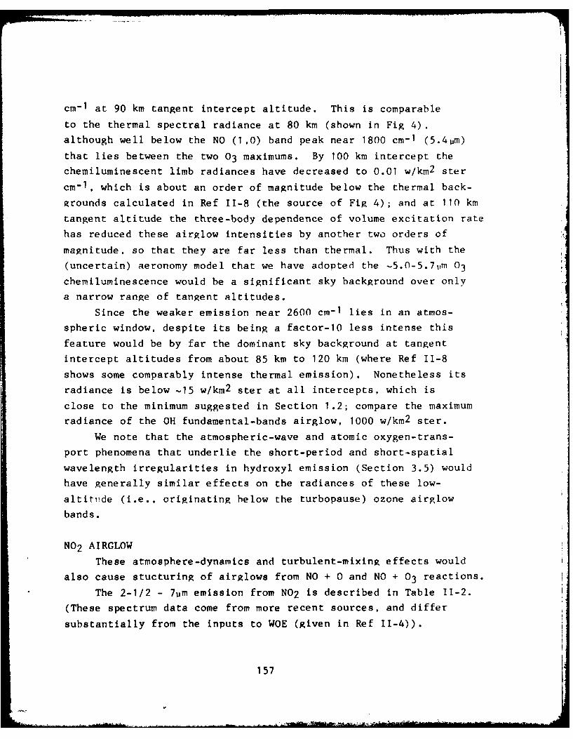
cm- 1 at 90 km tangent intercept altitude. This is comparable
to the thermal spectral radiance at 80 km (shown in Fig 4).
although well below the NO (1.0) band peak near 1800 cm-1 (5.4um)
that lies between the two 03 maximums. By 100 km intercept the
chemiluminescent limb radiances have decreased to 0.01 w/km2 ster
cm- 1 . which is about an order of magnitude below the thermal back-
grounds calculated in Ref 11-8 (the source of Fig 4); and at 110 km
tangent altitude the three-body dependence of volume excitation rate
has reduced these airglow intensities by another two orders of
magnitude, so that they are far less than thermal. Thus with the
(uncertain) aeronomy model that we have adopted the -5.0-5.7itm 03
chemiluminescence would be a significant sky background over only
a narrow range of tangent altitudes.
Since the weaker emission near 2600 cm -1 lies in an atmos-
spheric window, despite its being a factor-10 less intense this
feature would be by far the dominant sky background at tangent
intercept altitudes from about 85 km to 120 km (where Ref 11-8
shows some comparably intense thermal emission). Nonetheless its
radiance is below -15 w/km2 ster at all intercepts, which is
close to the minimum suggested in Section 1.2; compare the maximum
radiance of the OH fundamental-bands airglow, 1000 w/km 2 ster.
We note that the atmospheric-wave and atomic oxygen-trans-
port phenomena that underlie the short-period and short-spatial
wavelength irregularities in hydroxyl emission (Section 3.5) would
have generally similar effects on the radiances of these low-
altitude (i.e., originating below the turbopause) ozone airglow
bands.
NO 2 AIRGLOW
These atmosphere-dynamics and turbulent-mixing effects would
also cause stucturing of airglows from NO + 0 and NO + 03 reactions.
The 2-1/2 - 7um emission from N02 is described in Table 11-2.
(These spectrum data come from more recent sources, and differ
substantially from the inputs to WOE (given in Ref 11-4)).
1 57
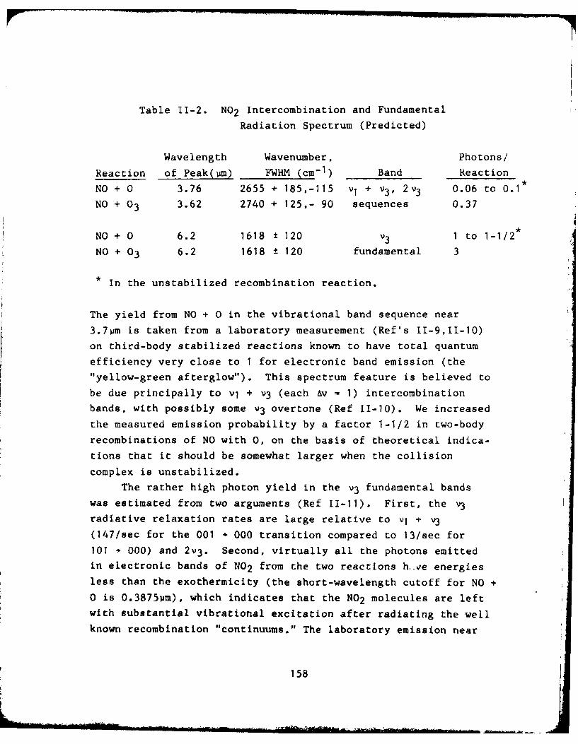
Table 11-2. NO2 Intercombination and Fundamental
Radiation Spectrum (Predicted)
Wavelength Wavenumber, Photons/
Reaction of Peak(um) FUHM (cm-i1 ) Band Reaction
NO + 0 3.76 2655 + 185,-115 v1 + v3 , 2v3 0.06 to 0.1*
NO + 03 3.62 2740 + 125,- 90 sequences 0.37
NO + 0 6.2 1618 ± 120 v3 1 to 1-1/2
NO + 03 6.2 1618 ± 120 fundamental 3
* In the unstabilized recombination reaction.
The yield from NO + 0 in the vibrational band sequence near
3.7om is taken from a laboratory measurement (Ref's 11-9,11-10)
on third-body stabilized reactions known to have total quantum
efficiency very close to 1 for electronic band emission (the"yellow-green afterglow"). This spectrum feature is believed to
be due principally to vI + v3 (each Av - 1) intercombination
bands, with possibly some v3 overtone (Ref 11-10). We increased
the measured emission probability by a factor 1-1/2 in two-body
recombinations of NO with 0, on the basis of theoretical indica-
tions that it should be somewhat larger when the collision
complex is unstabilized.
The rather high photon yield in the v3 fundamental bands
was estimated from two arguments (Ref 11-11). First, the v3radiative relaxation rates are large relative to vI + v3
(147/sec for the 001 + 000 transition compared to 13/sec for
101 + 000) and 2v3. Second, virtually all the photons emitted
in electronic bands of NO2 from the two reactions h..ve energies
less than the exothermicity (the short-wavelength cutoff for NO +
0 is 0.3875um), which indicates that the NO2 molecules are left
with substantial vibrational excitation after radiating the well
known recombination "continuums." The laboratory emission near
158

3.7um from NO + 03 is shifted to shorter wavelengths (Ref 11-10);
since less energy is available for vibrational excitation, we
have estimated a lower yield of v3 fundamental photons from
these reactions (93% of which result in NO2 in the ground
electronic state of N02 , Ref 11-12). In practice, NO + 03 re-
arrangement reactions make only a small contribution to the
total infrared radiances.
The effective two-body rate coefficient for NO + 0 recombina-
tion decreases with pressure above -50 km altitude (Ref 11-13).
In the absence of better information we adopt the (temperature)- 2
dependence observed in the high-pressure (third-body-stabilized)
limit, and as noted we have also increased the photon yields from
the unstabilized reactions. For NO + 03, we apply the rate
coefficient 2.1 x 10⁻¹² exp[-1450/T] from Ref 11-4. We adopt
again the Jacchia model atmosphere, along with the altitude
profiles of [NO] (which is an average of observations) and [03]
(which differ by about an order of magnitude between day and
night) that are used in AFGL's model of thermal radiance (Ref
11-8). For reference, the input data for our calculation of
NO2 chemiluminescence are given in Table 11-3 (the k's are
rate coefficients for the two reactions). We used the "average"
NO profile given in Ref 11-8; the factors-10 variations about
this mean that have been measured (as reviewed in Ref 11-14)
result in correspondingly large excursions from the mean airglow
radiances calculated.
Zenith column emission rates in the two airglow peaks in
Table 11-2 are then again the sum over altitude
J[NOJ {[OJ x(Rate coefficient x photons/reaction from Table 11-3)
+103] x(Rate coefficient from Table 11-3 x 0.37 or 3
photons/reaction)}.
In view of the low deactivation cross-sections reported in Ref
II-10 collisional quenching can be neglected at the altitudes
where NO2 is produced. The emission is dominated by the NO + 0
159
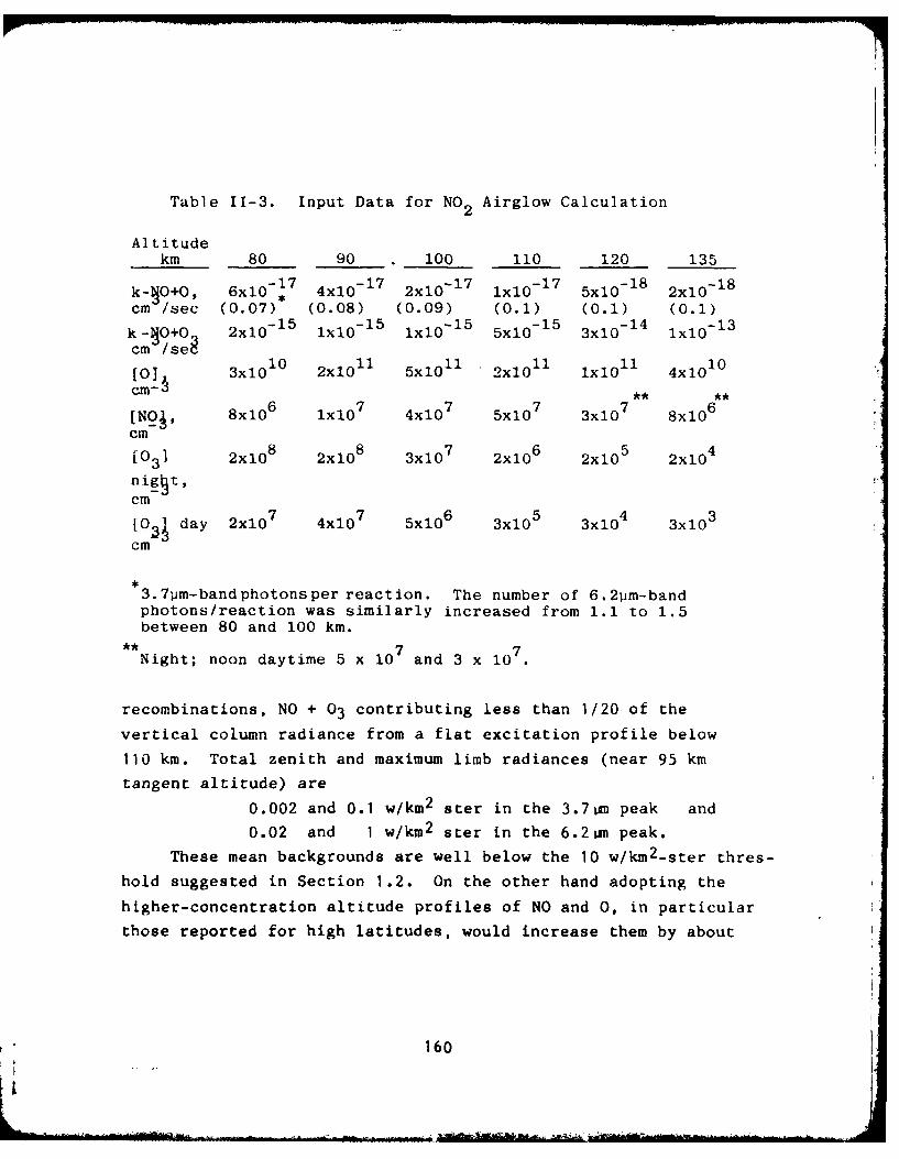
Table 11-3. Input Data for NO 2 Airglow Calculation
Altitudekm 80 90 100 110 120 135
k--O+OV 6x10 7 4x10¹⁷ 2x10 17 1x10⁻¹ 7 5xi0-18 2x10¹⁸
cm /sec (0.07) (0.08) (0.09) (0.1) (0.1) (0.1)
k- O+O 2xlO - 1 5 ixlO-15 IxlO 1 5 5xlO-15 3x1-14 IxlO-13
cm /sex
[0] 3x10 2xlO1 1 5x10 2x1 1 lxlO 4x10cm- ** **
[NOJ, 8x10 6 1x10 7 4x10 7 5x10 7 3x10 7 8x10 6
cm8 8 7 6 54[03) 2x10 2x10 3x10 2x10 2x10 2x10 4
nigqt,cm
[0 day 2x10 7 4x10 7 5x10⁶ 3x10 5 3x10 4 3x10 3
cm
3.71im-bandphotonsper reaction. The number of 6.2km-bandphotons/reaction was similarly increased from 1.1 to 1.5between 80 and 100 km.
**7 7Night; noon daytime 5 x 10 and 3 x 10
recombinations, NO + 03 contributing less than 1/20 of the
vertical column radiance from a flat excitation profile below
110 km. Total zenith and maximum limb radiances (near 95 km
tangent altitude) are
0.002 and 0.1 w/km2 ster in the 3.7 a peak and
0.02 and 1 w/km 2 ster in the 6.2in peak.
These mean backgrounds are well below the 10 w/km 2-ster thres-
hold suggested in Section 1.2. On the other hand adopting the
higher-concentration altitude profiles of NO and 0, in particular
those reported for high latitudes, would increase them by about
160

V
a factor 50, to 5 and 50 w/km 2 ster (or -0.015 and 0.15 w/km 2 -
ster cm-1 ) respectively in the limb. Like the 3.80m
(-2600 cm- 1 ) chemiluinescence of 03, the shorter-wavelength NO2
peak is weak compared to planned measurements experiments
thresholds but strong compared to the upper atmosphere's thermal
emission. With the yield of v3-fundamental photons adopted,
the airglow radiance in the 6 .2 wm band is more intense than
the thermal (largely, H2 0) emission shown in Ref 11-8 above
-90 km tangent intercept altitude. Moreover, it would be substan-
tially brighter in the apparently not-infrequent cases that
[NO] and [0] are significantly enhanced over the averages listed
in Table 11-3.
SUMMARY
Because of the large uncertainties in the photon yields and
emission spectra and the natural variability of reactant concen-
trations, intensities of the infrared airglows from 03 and N02 can
only be approximated. Clearly, further data are needed on excita-
tation/deexcitation rates, species profile systematics, and
actual limb radiances. With the aeronomy and model atmosphere
that we have adopted, chemiluminescence from these molecules
results in limb backgrounds at least comparable to thermal
broad wavenuber regions; in particular, both 03 and NO2 €overwveznrrgos32
fill in the the atmospheric window near 2600 cm-1 .
Spatial and temporal irregularities of these relatively
low-altitude airglows at all scales would be expected to be
generally similar to those of hydroxyl. The NO2 vibrational
band intensities are increased by auroral activity, with a
smaller effect on 03 because charged-particle impacts result
in only a small fractional increase in concentration of 0 atoms.
The long time scales of the recombination-airglow reactions
(-days), however, washes out the initial structure of auroral-
particle input.
161
REFERENCES
II-1. J.C. Gerard and C.A. Barth, J. Geophys. Res. 82, 674(1977).
11-2. W.T. Rawlins, G.B. Caledonia, and J.P. Kennealy,J. Geophys. Res. 86. 5247 (1981).
11-3. T.L. Stephens (Kaman-Tempo), Private communication(1982).
11-4. D.H. Archer, Further Requirements for Improved Pre-diction Capability: LWIR, DNA 5471F (31 Oct 80).
11-5. B.D. Green, W.T. Rawlins, and G.E. Caledonia, PhysicalSciences, Inc.. Report TR-296 (Feb 82).
11-6. R.E. Huie, J.J. Huron, and D.D. Davis, J. Phys. Chem 76,2653 (1972).
11-7. L.G. Jacchia. Smithsonian Astrophysical. ObservatoryReport 375. Cambridge. MA (1977).
II-R. T.C. DeRges and H.J.P. Smith, A High Altitude RadianceModel. AFGL-TR-77-0271 (30 Nov 77).
11-9. M.F. Golde. A.E. Roche, and F. Kaufman, J. Chem, Phys.59. 3953 (1973).
II-10. M.F. Golde and F. Kaufman, Chem. Phys. Lett. 29, 480(1974).
I-11. F. Kaufman (University of Pittsburgh). Privatecommunication (1982).
11-12. P.N. Clough and B.A. Thrush, Trans. Faraday Soc. 63,915 (1967).
11-13. F. Kaufman, The Air Afterglow Revisited, in Chemi-luminescence and Bioluminescence (ed's Cormier,Hercules, and Lee), Plenum, New York, 1973.
11-14. W. Swider in Proc. NATO Advanced Study Institute onAtmospheric Ozone (ed. A.C. Aikin), FAA-EE-80-20 (1980).
162
APPENDIX III
AURORAL INPUT-INTENSITY DISTRIBUTION DATA
FROM DYNAMICS EXPLORER
INTRODUCTION
As noted in Section 2, the spatial and temporal distribution
of auroral-particle energy input into measurements sight paths
is subject to considerable uncertainty because of the sparsity
of observational data. (The extreme complexity of' the underlying
geophysics precludes development of plausible predictive models.)
The data base to date consists principally of scanning-images
excited by particle impact taken from the sun-synchronous DMSP
satellites (the radiances are only semi-quantitative, and are
restricted to the limited (night) time period during which the
satellites pass over auroral latitudes), and from the ISIS
satellites (also low earth orbiting and sensitive only at night);
nadir UV radiometry from the S3-4 satellite (on which more
presently); groundbased all-sky camera network photographs;
some surveys from aircraft with all--sky cameras and ionosphere
sounders; and energy spectrums of the incoming particles measuredi
from low altitude orbiting satellites (including DMSP and IShS).
A systematic and self-contained set of energy inpit !' ux
data is now becoming available, from imaging photometers onr
NASA's Dynamics Explorer 1 Satellite (Ref's III-1, MI-2.. The
critical features of the experiment are
1) a highly eccentric, Molniya-type orbit
initially at 90' inclination, which
maintains the satellite over high latitudes
for most of each orbit when its apogee Is
near a geomagnetic pole;
2) measurement of radiance distributions over
an angular field larger than that subtended
by the auroral oval in six auroral emission
bands, including some in the ultraviolet from
163
which particle energy input rates in thesunlit atmosphere can be determined.
Thils combination of image field and spacecraft location proviaes
nearly continuous (actually, "time-lapse", as 10 mnn Is needed
to compose an image' ronitorilng of the particle energy input
occurrences and thieir spatial correlation over most or all of
tne oval, albeit at some sacrifice of spatial resolution. The
duration of the measurements Is determinea by the selected
satellites orbital precession and expectedi lifetime.
?EiFOR,'ANCE CAARACTEHISTICS
Dynamics Explorer is a followon to NASA's Atmospheric Explort-m
anid International Sun-Earth Explorer satellite programs. It
design d to probe s1multaneously the magnetospnere ano iosp:.,r,
to study coupling between the two regions and in partlcular tr,e
mechanism by which the energetic charged particles that excite
optLcal and infrared aurora are injected into the atmospherF-.
The two spatially-coordinated DE spacecraft were launchei from
Western Test Range at 0255 PDT on 03 Aug 81; DE-2 is in a low
altitu]e ('"ionosphere") orbit (1012 x 305 kin, -i01 min perlou),
tid [LE-I ("magnetosphere") in a coplanar 23,100 km (4.6 earth
radii) x 570 km orbit with _)440 min period.
Three 1/4' x 1/4°-IFOV photometers on DE-1 (Spin-Scan
Auroral Imagers, or alternatively, Global Auroral Imaging Photo-
meters, described in Ref 111-2) compose 300 x 120 0 -field radio-
metrically calibrated images. They are programmed for sensitivity
to the 0.3914wm N2 First Negative bands, 0.55774m 0i line, 0.6300m
!)i line, 0.i216vm hydrogen Lyman-a, 01 permitted lines between
0.130 and 0.136pm, or N 2 Lyman-Birge-Hopfield bands between about
0.13 and 0.171m. (Other wavelength-isolating filters can be
cycled into position to perform non-auroral measurements.) The
sunlit-sky background in the last two vacuum ultraviolet-
sensitivity bands is sufficiently low and spatially unvarying
164

(at least away from the atmosphere's limb) that particle energy
fluxes are measurable by day.
Intensity threshold without coadding picture elements is
about 1 kilorayleigh (109 photons/sec cm 2-coliznn). Spatial
resolution -- footprint of the photometers' fields -- is is 40 kj
when DE-1 is at 10,000 km altitude and 115 km (which is 1' of
latitude) at apogee. Thus spatial and intensity resolution have
been traded off against maintaining nearly continuous coverage
of the auroral oval (when apogee is over high latitudes). Some
early DE-l scanning images of substorm development that were
presented at an AGU meeting (Ref III-1), clearly show the
instrument's expected low spatial resolution and wide angular
coverage.
DE-1's apogee was placed initially over the north geographic
pole. Its orbit processes south at about 0.30 of latitude per
day, which moves the apogee over the south pole by April 1983.
Since the spatial distribution of charged particle input is
similar in conjugate hemispheres, occurrence statistics from
the southern auroral oval apply also to the northern oval.
Occurrence data will be available for all local times, as the
orbital period is not commensurate with the length of a day.
We note that a three-year lifetime of DE-1 would allow it to
survey auroral input distributions over about one quarter of a
solar cycle.
COMPLEMENTARY DATA FROM S3-4
UV atmospheric emissions have also been recently measured
by .1arrow-field photometers and spectrometers on USAF's polar-
orbiting satellite S3-4 (Ref 111-3), at wavelengths at which
daytime aurora is detectable. These data have much higher
spatial and intensity resolution because of the vehicle's low
orbital altitude (<260 kin); however, they are limited to the
times of its sun-synchronous crossings of the ovals and of
course lack the longitudinal coverage provided by DE-l's cross-
165

track scan. (That is, like particle counters the photo-
meters compose only one-dimensional "images."). Since S3-4
crosses the ovals near 1030 and 2230 LT it returns information
on the probabilities of input flux on both the dayside and the
(better-known) local midnight sector. It is also a source of
data on spatial structure at <1 km scale, which complement the
lower-resolution, more continuous radiance distributions from
Dynamics Explorer.
The auroral input flux rate is closely proportional to the
column intensities of the N2 Lyman-Birge-Hopfield bands as
well as the N First Negative bands. The First Negative bands
are of course detectable only at night, and their radiance distri-
bution is contaminated by backscattering from the lower atmosphere
and earth's surface. In contrast the ultraviolet L-B-H bands from
aurora become detectable against the zenith-sunlit sky when the
particle input rate is greater than about 2000 w/km 2 , and
their radiances have only a negligible backscatter component.
Further, the relative intensities of individual L-B-H bands (and
of the 01 lines) provide a measure of the characteristic energy
of the incoming particles (Ref 111-4; because of the wavelength
dependence of VUV absorption by atmospheric 02). At night
mean emission altitudes (for measuring energy input into into
slant sight paths) can be determined from the 0.6300 =/0.3914
column intensity ratios, as described in Section 2.4.1. Similarly,
the altitude profiles of energy deposition in the daytime can be
assessed from DE-I's ultraviolet image data.
ADMINISTRATIVE, SUMMARY
The Dynamics Explorer program is managed by NASA/Goddard
Space Flight Center. Data from the Spin-Scan Auroral Imager will
be treated separately from those from the 14 in-situ measuring,
non-imaging instruments on the two satellites; they are to be
preprocessed as described in Ref 111-2 and put on microfilm (and
166
other formats) for distribution to the program scientists. An
analysis of these imaging-photometer data from periods when
DE-I's apogee is at high northern or southern latitudes would
serve to determine probabilites of occurrence of auroral input
flux with time resolution of a few min and spatial resolution
(footprint) about 1 degree square at virtually all magnetic times.
REFERENCES
III-I. Trans. Am. Geophys. Un. 61, (1980) (general descriptionof satellites); Trans. Am. Geophys. Un. 62, 995-6 (1981)(Fall 1981 meeting abstracts outlining preliminary results).
111-2. L.A. Frank, J.D. Craven, K.L. Ackerson, M.R. English,R.H. Eather, and R.L. Carovillano, Space Sci. Inst. 5,369 (1981).
111-3. R.E. Huffman, F.J. LeBlanc, J.C. Larrabee, amd D.E. Pau3str,J. Geophys. Res. 85, 2201 (1980).
111-4. D.J. Strickland, J. R. Jasperse, and J.A. Whalen, Trans.Am. Geophys. Un. 62 977 (1981).
167

I