structure of the dualsphysics code

Structure of the DualSPHysics code

Dr José Manuel Domínguez Alonso

[email protected]

Dr George Fourtakas

[email protected]

mailto:[email protected]

mailto:[email protected]

Outline

1. DualSPHysics

1.1. Origin of DualSPHysics

1.2. Why GPUs?

1.3. DualSPHysics project

2. SPH formulation

3. Structure of code

3.1. Stages of simulation

3.2. Source files

3.3. Object-Oriented Programming

3.4. Execution diagram

4. Input & output files

5. Test cases online

6. Novelties in next release v4.0

DualSPHysics Users Workshop 2015, 8-9 September 2015, Manchester (United Kingdom)

SPHysics is a numerical SPH solver developed for the study of free-surface problems.

It is a code written in Fortran90 with numerous options (different kernels, several

boundary conditions, etc.), which has already demonstrated high accuracy in several

validations with experimental results but it is too slow to apply to large domains.

The DualSPHysics code was created starting from SPHysics.



The problem:

• SPH REQUIRES HIGH COMPUTATIONAL COST THAT INCREASES WHEN

INCREASING THE NUMBER OF PARTICLES

• THE SIMULATION OF REAL PROBLEMS REQUIRES HIGH RESOLUTION WHICH

IMPLIES SIMULATING MILLIONS OF PARTICLES

IT WAS NECESSARY TO INCREASE THE PERFORMACE OF THE CODE A FACTOR

x100

Classic options:

- OpenMP: Distribute the workload among all CPU cores (≈4x)

- MPI: Combines the power of multiple machines connected via network (high cost).

New option:

- GPU: Graphics cards with a high parallel computing power (cheap and accessible).



Advantages: GPUs provide the necessary computational power with very low cost and

without expensive infrastructures.

Drawbacks: An efficient and full use of the capabilities of the GPUs is not

straightforward.

Graphics Processing Units (GPUs)

are powerful parallel processors

originally designed for graphics

rendering.

Due to the development of the video

games market and multimedia, their

computing power has increased

much faster than CPUs.

Now, GPUs can be used for general

purpose applications, achieving

speedups of x100 or more.

1.2. Why GPUs?


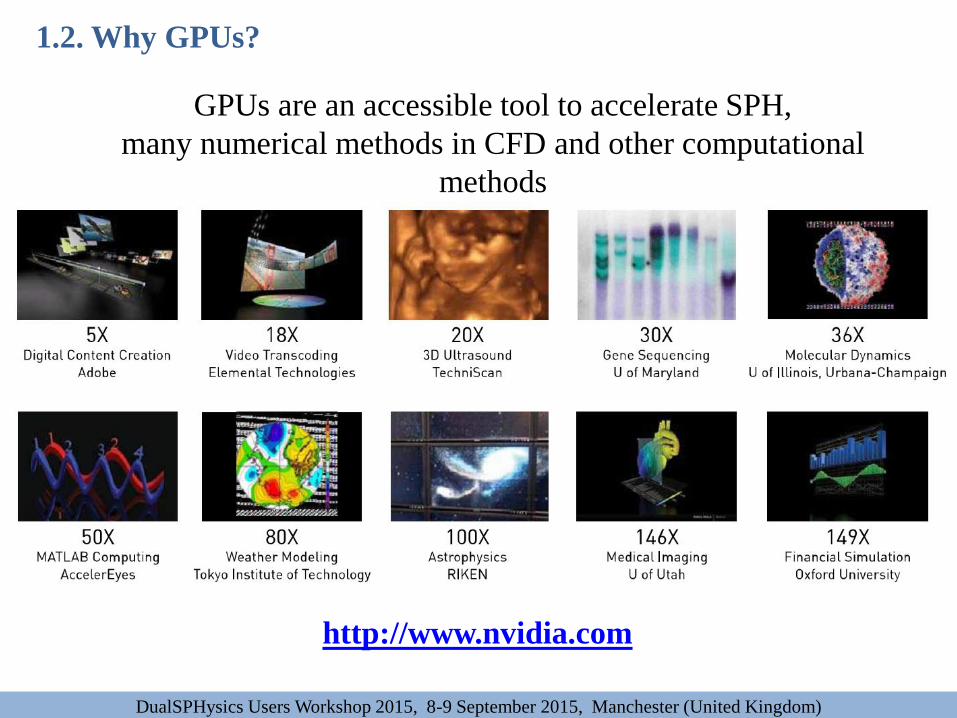
GPUs are an accessible tool to accelerate SPH,

many numerical methods in CFD and other computational

methods

http://www.nvidia.com

1.2. Why GPUs?


http://www.nvidia.com/

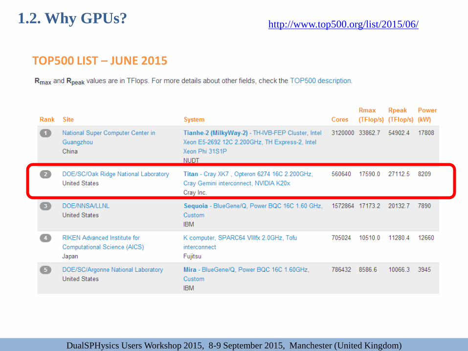
http://www.top500.org/list/2015/06/

1.2. Why GPUs?


TOP500 LIST – JUNE 2015



Why two implementations?

This code can be used on machines with and without a GPU.

It allows us to make a fair and realistic comparison between CPU and GPU.

Some algorithms are complex and it is easy to make errors - difficult to detect. So they

are implemented twice and we can compare results.

It is easier to understand the code in CUDA when you can see the same code in C++.

Drawback: It is necessary to implement and to maintain two different codes.

First version in late 2009.

It includes two implementations:

- CPU: C++ and OpenMP.

- GPU: CUDA.

Both implementations optimized for

best performance for each

architecture.




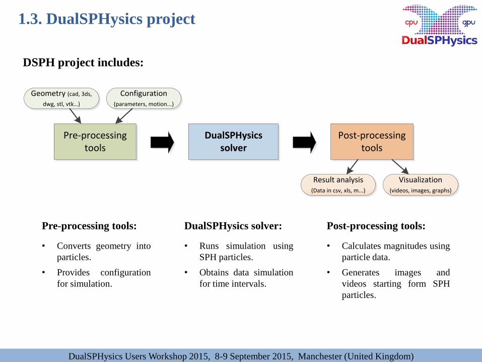
Pre-processing tools

DualSPHysics solver

Post-processing tools

Geometry (cad, 3ds,

dwg, stl, vtk…)

Configuration (parameters, motion...)

Visualization(videos, images, graphs)

Result analysis(Data in csv, xls, m...)

DSPH project includes:

Pre-processing tools:

• Converts geometry into

particles.

• Provides configuration

for simulation.

DualSPHysics solver:

• Runs simulation using

SPH particles.

• Obtains data simulation

for time intervals.

Post-processing tools:

• Calculates magnitudes using

particle data.

• Generates images and

videos starting form SPH

particles.


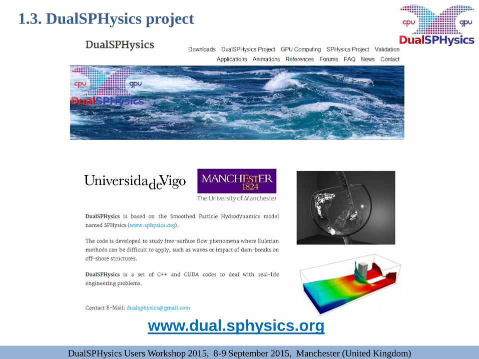
www.dual.sphysics.org



Prof. Moncho Gómez Gesteira

Dr Alejandro J.C. Crespo

Dr Jose M. Domínguez

Dr Anxo Barreiro

Orlando G. Feal

Carlos Alvarado

Dr Benedict D. Rogers

Dr Athanasios Mokos

Dr Georgios Fourtakas

Dr Stephen Longshaw

Abouzied Nasar

Prof. Peter Stansby

Dr Renato Vacondio

Prof. Paolo Mignosa

Dr Corrado Altomare

Dr Tomohiro Suzuki

Prof. Rui Ferreira

Dr Ricardo Canelas

Dr Xavier Gironella

Andrea Marzeddu

People working on DualSPHysics project:



Outline

1. DualSPHysics


1.2. Why GPUs?


2. SPH formulation



3.2. Source files







• Time integration scheme: o Verlet [Verlet, 1967]

o Symplectic [Leimkhuler, 1996]

• Variable time step [Monaghan and Kos, 1999]

• Smoothing kernel functions: o Cubic Spline kernel [Monagham and Lattanzio, 1985]

o Wendland kernel [Wendland, 1995]

• Weakly compressible approach using Tait’s equation of state

• Density filter: o Shepard filter [Panizzo, 2004]

o Delta-SPH formulation [Molteni and Colagrossi, 2009]

• Viscosity treatments: o Artificial viscosity [Monaghan, 1992]

o Laminar viscosity + SPS turbulence model [Dalrymple and Rogers, 2006]

• Dynamic boundary conditions [Crespo et al., 2007]

• Floating objects [Monaghan et al., 2003]

• Periodic open boundaries

2. SPH formulation: DualSPHysics v3


Outline

1. DualSPHysics


1.2. Why GPUs?


2. SPH formulation



3.2. Source files







System update (SU):

Time integration is performed using the values

of computed forces, the particles field variables

are updated for the next iteration of the

simulation.

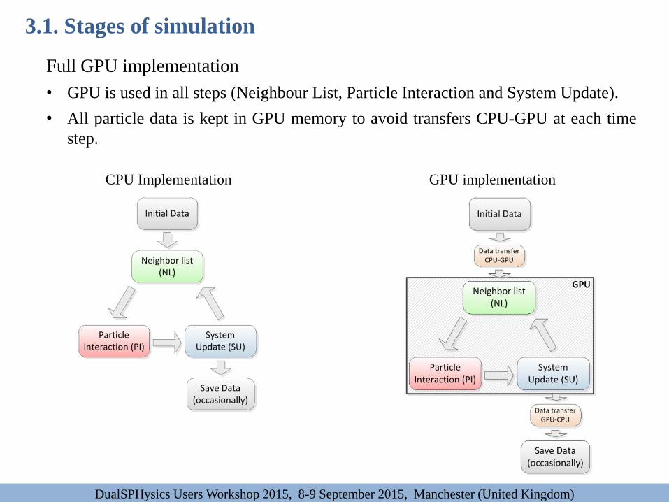
For the implementation of SPH, the code is organised in 3 main steps that are repeated

each time step till the end of the simulation.

Initial Data

Neighbour List (NL)

Particle Interaction (PI)

System Update (SU)

Save Data (occasionally)

Neighbour list (NL):

Particles are grouped in cells and reordered to

optimise performance (memory access).



ncx

2h

2h ncz

Particle interactions (PI):

Forces between particles are computed, solving

momentum and continuity equations.

This step takes more than 95% of execution time.

CPU Implementation GPU implementation

Full GPU implementation

• GPU is used in all steps (Neighbour List, Particle Interaction and System Update).

• All particle data is kept in GPU memory to avoid transfers CPU-GPU at each time

step.



3.2. Source files


20

21)2(4

1

104

3

2

31

)( 3

32

R

RR

RRR

aRW d

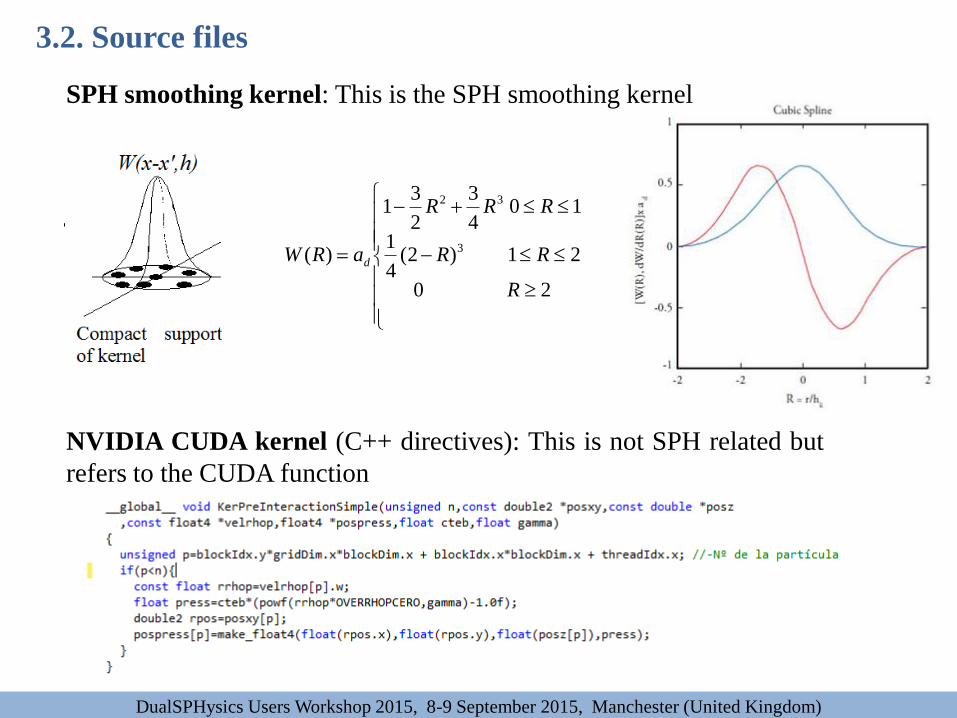
SPH smoothing kernel: This is the SPH smoothing kernel

NVIDIA CUDA kernel (C++ directives): This is not SPH related but

refers to the CUDA function

3.2. Source files

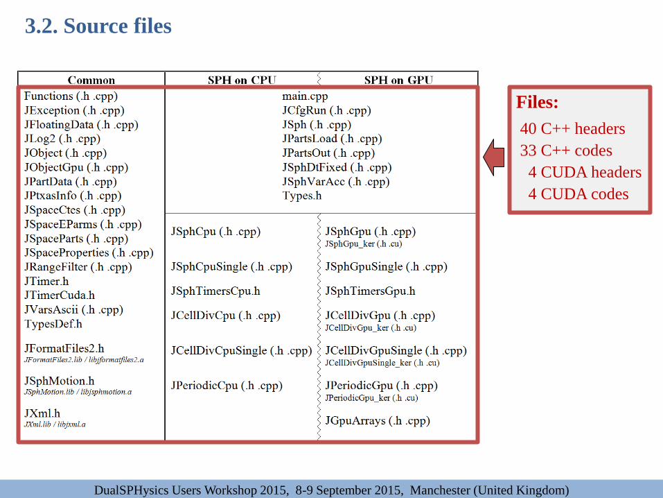
Files:

40 C++ headers

33 C++ codes

4 CUDA headers

4 CUDA codes


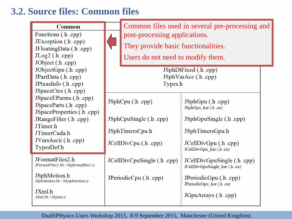
Common files used in several pre-processing and

post-processing applications.

They provide basic functionalities.

Users do not need to modify them.


3.2. Source files: Common files

Precompiled code in libraries.

Common files used in several pre-processing and

post-processing applications.

They provide basic functionalities.


3.2. Source files: Precompiled files

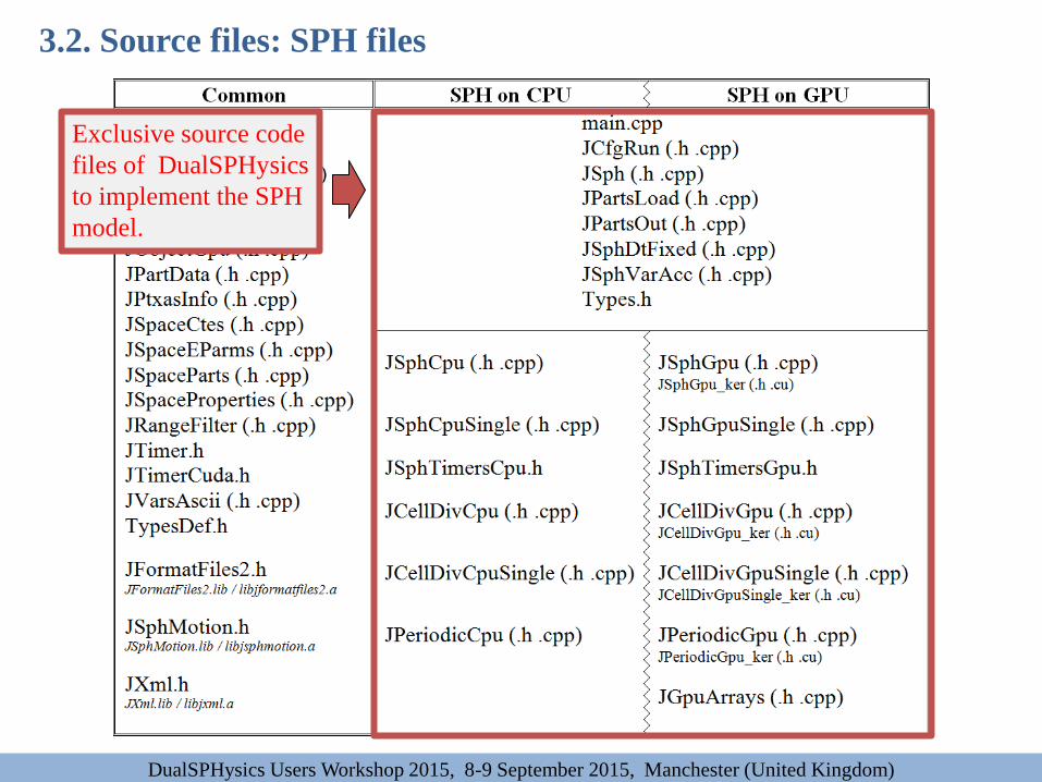
Exclusive source code

files of DualSPHysics

to implement the SPH

model.


3.2. Source files: SPH files

Code used in CPU and

GPU implementation.

Exclusive code for

CPU implementation.

Exclusive code

for GPU.


3.2. Source files: SPH files

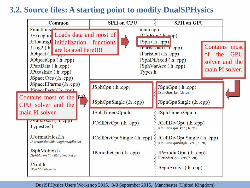
Loads data and most of

initialization functions

are located here!!!!

Contains most of the

CPU solver and the

main PI solver.

Contains most

of the GPU

solver and the

main PI solver.


3.2. Source files: A starting point to modify DualSPHysics

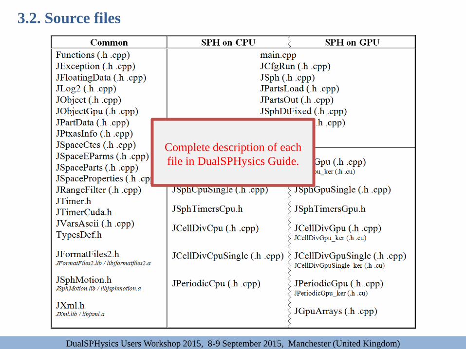
Complete description of each

file in DualSPHysics Guide.


3.2. Source files



Diagram main classes

DualSPHysics uses Object-Oriented Programming (OOP) to organise the code.

However, the particles data is stored in arrays to improve the performance.

Class name matches the file name.

JSphCpu

JSphCpuSingle

JCellDivCpu

JCellDivCpuSingle

JSph

JSphGpu

JSphGpuSingle

JCellDivGpu

JCellDivGpuSingle

JPeriodicCpu JPeriodicGpu

JLog2::Init

New JSphCpuSingle New JSphGpuSingle

Delete objects

END

MAIN

JSphGpuSingle::RunJSphCpuSingle::Run

JCfgRun::LoadArgv

3.4. Execution diagram: Main


The execution of DualSPHysics begins in function main() in file main.cpp

Loads parameters from

command line

Initializes log file

Creates object for execution

on Cpu or Gpu

Executes method Run() of

SPH object to start simulation

Deletes objects and frees

memory


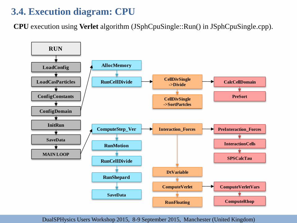
CPU execution using Verlet algorithm (JSphCpuSingle::Run() in JSphCpuSingle.cpp).

LoadConfig

LoadCasParticles

ConfigConstants

InitRun

SaveData

MAIN LOOP

ComputeStep_Ver

RunMotion

RunCellDivide

RunShepard

SaveData

Interaction_Forces

SPSCalcTau

DtVariable

RunFloating

RUN

ConfigDomain

ComputeVerlet

InteractionCells

PreInteraction_Forces

ComputeRhop

ComputeVerletVars

AllocMemory

RunCellDivideCellDivSingle

->Divide

CellDivSingle

->SortPartcles

PreSort

CalcCellDomain

3.4. Execution diagram: CPU


CPU execution using Symplectic algorithm (JSphCpuSingle::Run() in JSphCpuSingle.cpp).

LoadConfig

LoadCasParticles

ConfigConstants

InitRun

SaveData

MAIN LOOP

ComputeStep_Sym

PREDICTOR

RunMotion

RunCellDivide

RunShepard

SaveData

Interaction_Forces

SPSCalcTauDtVariable

RunFloating

RUN

ConfigDomain

ComputeSymplecticPre

InteractionCells


ComputeRhop

AllocMemory

RunCellDivideCellDivSingle

->Divide

CellDivSingle

->SortPartcles

PreSort

CalcCellDomain

ComputeStep_Sym

CORRECTOR

Interaction_Forces

SPSCalcTau

RunFloating

ComputeSymplecticCorr

InteractionCells


ComputeRhopEpsilon

RunCellDivide

DtVariable

3.4. Execution diagram: CPU


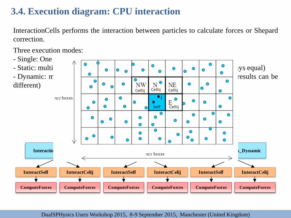
InteractionCells performs the interaction between particles to calculate forces or Shepard

correction.

Three execution modes:

- Single: One execution thread

- Static: multi-thread with OpenMP using static schedule (the results are always equal)

- Dynamic: multi-thread with OpenMP using dynamic schedule (faster but results can be

different)

InteractionCells<INTER_Forces>

<INTER_ForcesCorr>

InteractionCells_Single

InteractCelijInteractSelf

ComputeForcesComputeForces

InteractionCells_Static



InteractionCells_Dynamic



3.4. Execution diagram: CPU interaction


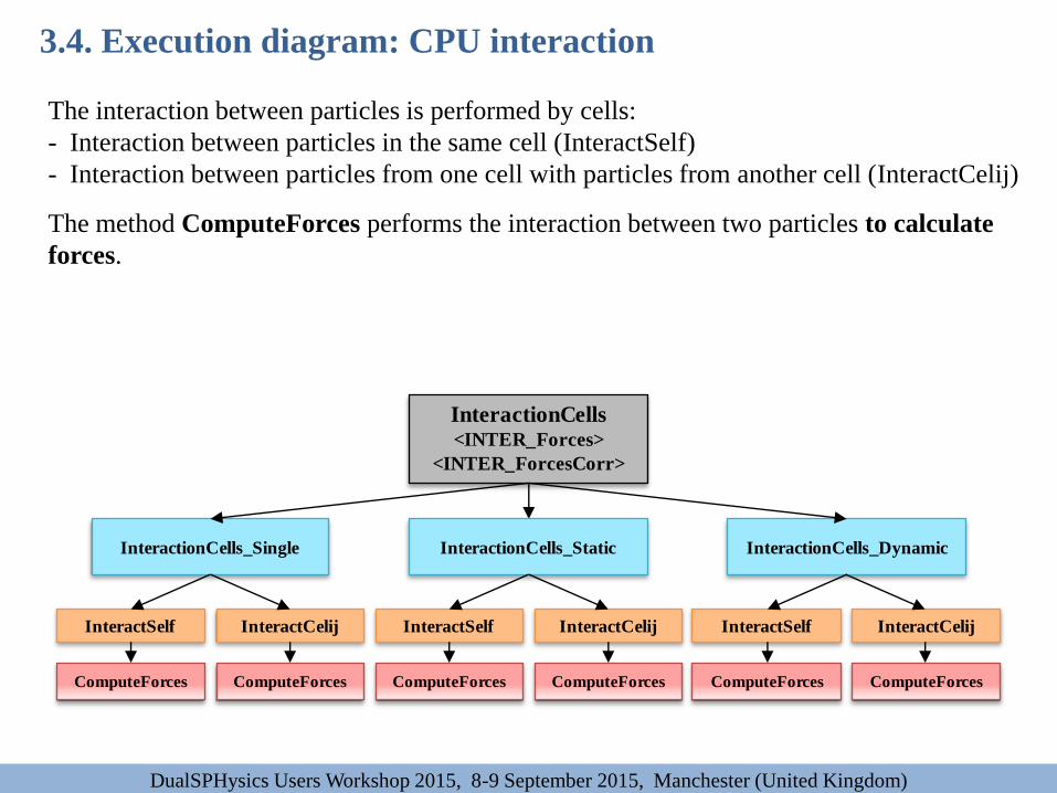
The interaction between particles is performed by cells:

- Interaction between particles in the same cell (InteractSelf)

- Interaction between particles from one cell with particles from another cell (InteractCelij)

The method ComputeForces performs the interaction between two particles to calculate

forces.

InteractionCells<INTER_Forces>

<INTER_ForcesCorr>












The interaction between particles is performed by cells:

- Interaction between particles in the same cell (InteractSelf)

- Interaction between particles from one cell with particles from another cell (InteractCelij)

The method ComputeForces performs the interaction between two particles to calculate

forces.

The method ComputeForcesShepard performs the interaction between two particles to

calculate Shepard correction.

InteractionCells<INTER_Shepard>



ComputeForcesShepardComputeForcesShepard









GPU execution using Verlet algorithm (similar to CPU execution).

LoadConfig

LoadCasParticles

ConfigConstants

InitRun

SaveData

MAIN LOOP

ComputeStep_Ver

RunMotion

RunCellDivide

RunShepard

SaveData

Interaction_Forces

SPSCalcTau DtVariable

RunFloating

RUN

ConfigDomain

ComputeVerlet

Interaction_Forces


FtCalcOmega

ComputeStepVerlet

AllocGpu

MemoryParticles

RunCellDivide

CellDivSingle

->Divide

CellDivSingle

->SortBasicArraays

PreSort

CalcCellDomainAllocCpu

MemoryParticles

ParticlesDataUp CellDivSingle

->CheckPartclesOut

Sort

CalcBeginEndCell

SelecDevice

FtUpdate

MoveLinBound

MoveMatBound

PreInteraction_Shepard

Interaction_Shepard

PosInteraction_Shepard

PreInteractionVars_Forces

PreInteractionVars_Shepard

PosInteraction_Forces

3.4. Execution diagram: GPU


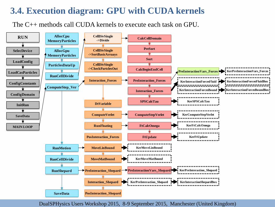
The C++ methods call CUDA kernels to execute each task on GPU.

LoadConfig

LoadCasParticles

ConfigConstants

InitRun

SaveData

MAIN LOOP

ComputeStep_Ver

RunMotion

RunCellDivide

RunShepard

SaveData

Interaction_Forces

SPSCalcTau DtVariable

RunFloating

RUN

ConfigDomain

ComputeVerlet

Interaction_Forces


FtCalcOmega

ComputeStepVerlet

AllocGpu

MemoryParticles

RunCellDivide

CellDivSingle

->Divide

CellDivSingle

->SortBasicArraays

PreSort

CalcCellDomainAllocCpu

MemoryParticles

ParticlesDataUp CellDivSingle

->CheckPartclesOut

Sort

CalcBeginEndCell

SelecDevice

FtUpdate

MoveLinBound

MoveMatBound

PreInteraction_Shepard

Interaction_Shepard

PosInteraction_Shepard

PreInteractionVars_Forces KerPreInteractionVars_Forces

KerInteractionForcesFluid

KerSPSCalcTau

KerComputeStepVerlet

KerFtCalcOmega

KerFtUpdate

KerMoveLinBound

KerMoveMatBound

PreInteractionVars_Shepard KerPreInteraction_Shepard

KerPreInteraction_Shepard

PosInteraction_Forces

KerInteractionShepardBox

KerInteractionForcesFluidBox

KerInteractionForcesBound KerInteractionForcesBoundBox

3.4. Execution diagram: GPU with CUDA kernels

Outline

1. DualSPHysics


1.2. Why GPUs?


2. SPH formulation


3.1. Steps of simulation

3.2. Source files







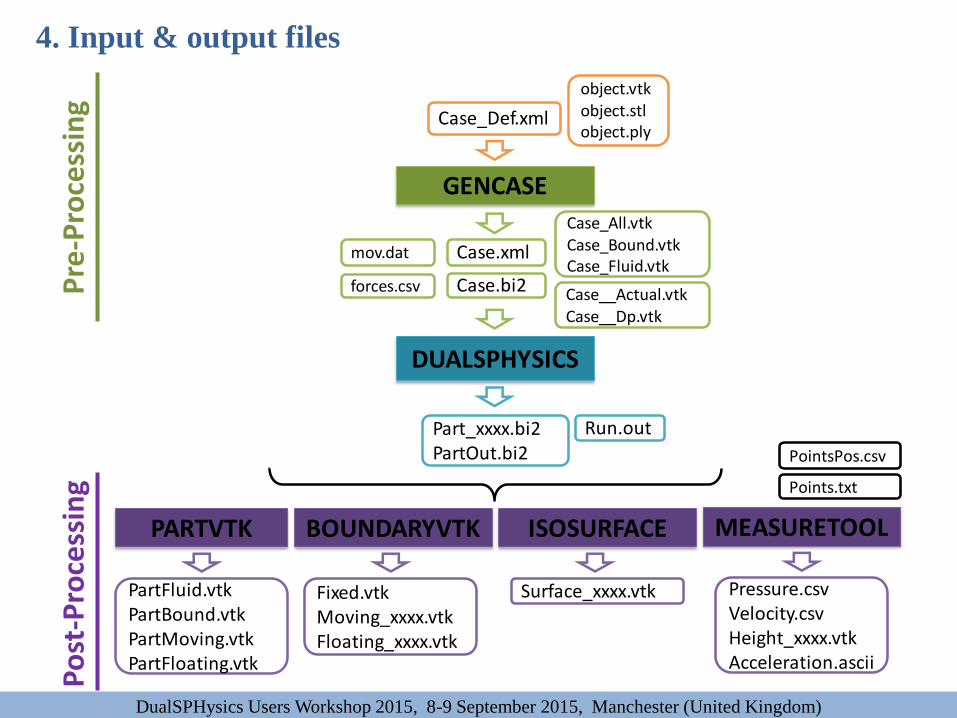
GENCASE

Case_Def.xml

object.vtkobject.stlobject.ply

DUALSPHYSICS

Run.outPart_xxxx.bi2PartOut.bi2

Case_All.vtkCase_Bound.vtkCase_Fluid.vtk

Case__Actual.vtkCase__Dp.vtk

Case.xml

Case.bi2

mov.dat

forces.csv

BOUNDARYVTKPARTVTK MEASURETOOL

Points.txt

Fixed.vtkMoving_xxxx.vtkFloating_xxxx.vtk

PartFluid.vtkPartBound.vtkPartMoving.vtkPartFloating.vtk

Pressure.csvVelocity.csvHeight_xxxx.vtkAcceleration.ascii

ISOSURFACE

Surface_xxxx.vtk

PointsPos.csv



Po

st-P

roce

ssin

g

P

re-P

roce

ssin

g

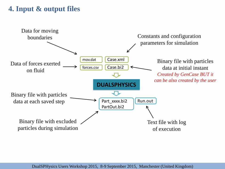
DUALSPHYSICS


Case.xml

Case.bi2

mov.dat

forces.csv



Data for moving

boundaries

Data of forces exerted

on fluid

Constants and configuration

parameters for simulation

Binary file with particles

data at initial instant Created by GenCase BUT it

can be also created by the user

Text file with log

of execution

Binary file with particles

data at each saved step

Binary file with excluded

particles during simulation


4. Input & output files: Format files

DUALSPHYSICS


Case.xml

Case.bi2

mov.dat

forces.csv

DUALSPHYSICS


Case.xml

Case.bi2

mov.dat

forces.csv

DUALSPHYSICS


Case.xml

Case.bi2

mov.dat

forces.csv

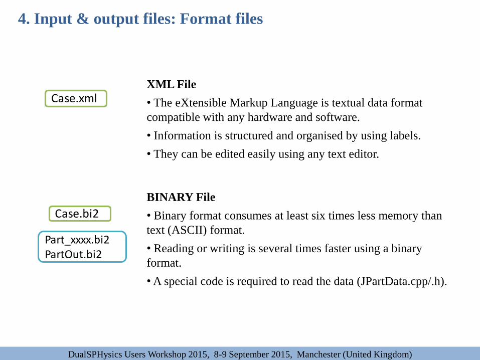
XML File

• The eXtensible Markup Language is textual data format

compatible with any hardware and software.

• Information is structured and organised by using labels.

• They can be edited easily using any text editor.

BINARY File

• Binary format consumes at least six times less memory than

text (ASCII) format.

• Reading or writing is several times faster using a binary

format.

• A special code is required to read the data (JPartData.cpp/.h).

Outline

1. DualSPHysics


1.2. Why GPUs?


2. SPH formulation



3.2. Source files







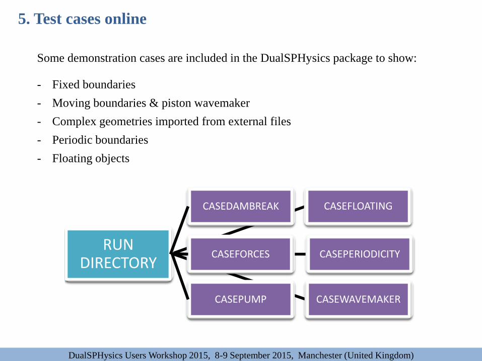
Some demonstration cases are included in the DualSPHysics package to show:

- Fixed boundaries

- Moving boundaries & piston wavemaker

- Complex geometries imported from external files

- Periodic boundaries

- Floating objects

EXECS

HELP

MOTION

DualSPHysicsCaseTemplate.xmlHELP_GenCase.out, HELP_DualSPHysics.out, HELP_BoundaryVTK.out, HELP_IsoSurface.out,HELP_PartVTK.out, HELP_MeasureTool.outXML_examples

GenCaseDualSPHysics + dll’s or lib’sDualSPHysics_ptxasinfoIsoSurfaceBoundaryVTKPartVTKMeasureTool

Motion.batMotion01.xml, Motion02.xml…, Motion08.xmlmotion08mov_f3.out

SOURCECode_Documentation

Source (+Libs)DualSPHysics_v3ToVTK

DualSPHysics_v3

RUN DIRECTORY

CASEDAMBREAK CASEFLOATING

CASEFORCES CASEPERIODICITY

CASEPUMP CASEWAVEMAKER



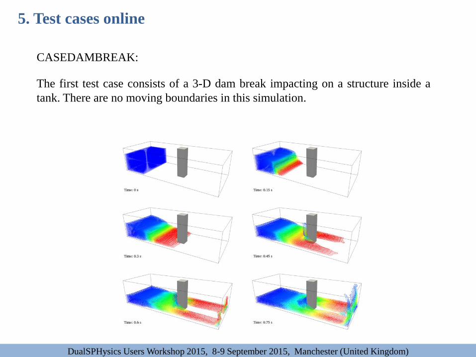
CASEDAMBREAK:

The first test case consists of a 3-D dam break impacting on a structure inside a

tank. There are no moving boundaries in this simulation.



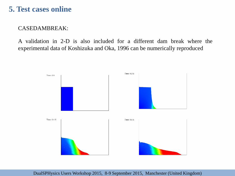
CASEDAMBREAK:

A validation in 2-D is also included for a different dam break where the

experimental data of Koshizuka and Oka, 1996 can be numerically reproduced



CASEFLOATING:

A floating box moves due to waves generated with a piston



CASEFLOATING:

The 2-D case of fluid-structure interaction is also provided. The text files included

in the folder contains the experimental displacement and velocity of experiments

in Fekken, 2004 and Moyo and Greenhow, 2000.



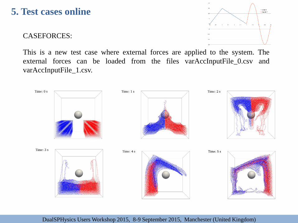
CASEFORCES:

This is a new test case where external forces are applied to the system. The

external forces can be loaded from the files varAccInputFile_0.csv and

varAccInputFile_1.csv.



CASEPERIODICITY:

This test case is an example of periodicity applied to 2D case where particles that

leave the domain through the right side are introduced through the left side with

the same properties but where the vertical position can change (with an increase

of +0.3 in Z-position).



CASEPUMP:

This 3D test case loads an external model of a pump with a fixed

(pump_fixed.vtk) and a moving part (pump_moving.vtk). The moving part

describes a rotational movement and the reservoir is pre-filled with fluid particles.



CASEWAVEMAKER:

CaseWavemaker simulates several waves breaking on a numerical beach. A

wavemaker is performed to generate and propagate the waves. In this test case, a

sinusoidal movement is imposed to the boundary particles of the wavemaker



Outline

1. DualSPHysics


1.2. Why GPUs?


2. SPH formulation



3.2. Source files







1) New CPU structure that mimics the GPU threads.

2) New GPU structure with the code better organized

Easy to follow and modify by the user.

3) Double precision implementation; several options.

4) Floating bodies formulation is corrected.

5) Delta-SPH of Molteni&Colagrossi plus others (to be confirmed)

6) Shifting algorithm

7) New wave generation (regular, irregular by given H/Hs, T/Tp and depth)

8) Source code of DEM (Discrete Element Method )

9) Multi-phase liquid-sediment solver release v3.2 (September 2015)

Check the website for news / releases / info



structure of the dualsphysics code

Documents