structured prediction cascades

916

Structured Prediction Cascades

David Weiss and Ben TaskarUniversity of Pennsylvania

Abstract

Structured prediction tasks pose a fundamen-tal trade-off between the need for model com-plexity to increase predictive power and thelimited computational resources for inferencein the exponentially-sized output spaces suchmodels require. We formulate and developstructured prediction cascades: a sequenceof increasingly complex models that progres-sively filter the space of possible outputs. Werepresent an exponentially large set of fil-tered outputs using max marginals and pro-pose a novel convex loss function that bal-ances filtering error with filtering efficiency.We provide generalization bounds for theseloss functions and evaluate our approach onhandwriting recognition and part-of-speechtagging. We find that the learned cascadesare capable of reducing the complexity of in-ference by up to five orders of magnitude, en-abling the use of models which incorporatehigher order features and yield higher accu-racy.

1 Introduction

The trade-off between approximation and estimationerror is fundamental in learning complex predictionmodels. In structured prediction tasks, such as part-of-speech tagging, machine translation and gene pre-diction, the factor of computation time also plays animportant role as models with increasing complexityof inference are considered. For example, a first orderconditional random field (CRF) (Lafferty et al., 2001)is fast to evaluate but may not be an accurate modelfor phoneme recognition, while a fifth order model ismore accurate, but prohibitively expensive for bothlearning and prediction. (Model complexity can also

Appearing in Proceedings of the 13th International Con-ference on Artificial Intelligence and Statistics (AISTATS)2010, Chia Laguna Resort, Sardinia, Italy. Volume 9 ofJMLR: W&CP 9. Copyright 2010 by the authors.

lead to overfitting problems due the sparseness of thetraining data. We do not specifically address this prob-lem in our paper other than judiciously regularizingmodel parameters.)

In practice, model complexity is limited by computa-tional constraints at prediction time, either explicitlyby the user or implicitly because of the limits of avail-able computation power. We therefore need to balanceexpected error with inference time. A common solu-tion is to use heuristic pruning techniques or approx-imate search methods in order to make higher ordermodels feasible. While it is natural and commonplaceto prune graphical model state space, the problem ofexplicitly learning to control the error/computationtradeoff has not been addressed. In this paper, we for-mulate the problem of learning a cascade of models ofincreasing complexity that progressively filter a givenstructured output space, minimizing overall error andcomputational effort at prediction time according to adesired tradeoff. The contributions of this paper are:

• A novel convex loss function specifically gearedfor learning to filter accurately and effectively.

• A simple online algorithm for minimizing this lossusing standard inference methods.

• Theoretical analysis of generalization of the cas-cade (in terms of both accuracy and efficiency).

• Evaluation on two large-scale applications: hand-writing recognition and part-of-speech tagging.

2 Related Work

Heuristic methods for pruning the search space of out-puts have been exploited in many natural languageprocessing and computer vision tasks. For part-of-speech tagging, perhaps the simplest method is to limitthe possible tags for each word to those only seen as itslabels in the training data. For example, the MXPOSTtagger (Ratnaparkhi, 1996) and many others use thistechnique. In our experiments, we compare to thissimple trick and show that our method is much moreaccurate and effective in reducing the output space. Inparsing, the several works (Charniak, 2000; Carreraset al., 2008; Petrov, 2009) use a “coarse-to-fine” idea

917


closely related to ours: the marginals of a simple con-text free grammar or dependency model are used toprune the parse chart for a more complex grammar.We also compare to this idea in our experiments. Thekey difference with our work is that we explicitly learna sequence of models tuned specifically to filter thespace accurately and effectively. Unlike the work ofPetrov (2009), however, we do not learn the structureof the hierarchy of models but assume it is given bythe designer.

It is important to distinguish the approach proposedhere, in which we use exact inference in a reduced out-put space, with other approximate inference techniquesthat operate in the full output space (e.g., Druck et al.(2007), Pal et al. (2006)). Because our approach is or-thogonal to such approximate inference techniques, itis likely that the structured pruning cascades we pro-pose could be combined with existing methods to per-form approximate inference in a reduced output space.

Our inspiration comes partly from the cascade classi-fier model of Viola and Jones (2002), widely used forreal-time detection of faces in images. In their work, awindow is scanned over an image in search of faces anda cascade of very simple binary classifiers is trained toweed out easy and frequent negative examples earlyon. In the same spirit, we propose to learn a cascadeof structured models of increasing order that weed outeasy incorrect assignments early on.

3 Structured Prediction Cascades

Given an input space X , output space Y, and a train-ing set S = {

⟨x1, y1

⟩, . . . , 〈xn, yn〉} of n independent

and identically-distributed (i.i.d.) random samplesfrom a joint distribution D(X,Y ), the standard super-vised learning task is to learn a hypothesis h : X 7→ Ythat minimizes the expected loss ED [L (h(x), y)] forsome non-negative loss function L : Y × Y → R+.

We consider the case of structured classification whereY is a `-vector of variables and Y = Y1 × · · · × Y`.In many settings, the number of random variables Ydiffers depending on input X (for example, length ofthe sentence in part of speech tagging), but for sim-plicity of notation, we assume a fixed number ` here.We denote the components of y as y = {y1, . . . , y`},where yi ∈ {1, . . . ,K}. The linear hypothesis class weconsider is of the form:

hw(x) = argmaxy∈Y

w>f(x, y) (1)

where w ∈ Rp is a vector of parameters and f : X ×Y 7→ Rp is a function mapping (x, y) pairs to a setof p real-valued features. We further assume that fdecomposes over a set of cliques C ⊆ P{X,Y } (where

P is a powerset):

w>f(x, y) =∑c∈C

w>fc(x, yc). (2)

Above, yc is an assignment to the subset of Y vari-ables in the clique c and we will use Yc to refer tothe set all assignments to the clique. By consideringdifferent cliques over X and Y , f can represent ar-bitrary interactions between the components of x andy. Thus, evaluating hw(x) is not always tractable, andcomputational resources limit the expressiveness of thefeatures that can be used.

For example, a first order Markov sequence model hascliques {Yi, Yi+1, X} to score features depending onemissions {X,Yi} and transitions {Yi, Yi+1}:

w>f(x, y) =∑i=1

w>fi(x, yi, yi+1). (3)

For the first order model, evaluating (1) requiresO(K2`) time using the Viterbi decoding algorithm.For an order-d Markov model, with cliques over{yi, . . . , yi+d, x}, inference requires O(kd+1`) time.

Several structured prediction methods have beenproposed for learning w, such as conditional ran-dom fields (Lafferty et al., 2001), structured percep-tron (Collins, 2002), hidden Markov support vectormachines (Altun et al., 2003) and max-margin Markovnetworks (Taskar et al., 2003). Our focus here is in-stead on learning a cascade of increasingly complexmodels in order to efficiently construct models thatwould otherwise be intractable.

3.1 Cascaded inference with max-marginals

We will discuss how to learn a cascade of models inSection 4, but first we describe the inference proce-dure. The basic notion behind our approach is verysimple: at each level of the cascade, we receive as in-put a set of possible clique assignments correspondingto the cliques of the current level. Each level furtherfilters this set of clique assignments and generates aset of possible clique assignments which are passed asinput to the next level. Note that each level is able toprune further than the preceding level because it canconsider higher-order interactions. At the end of thecascade, the most complex model chooses a single pre-diction as usual, but it needs only consider the cliqueassignments that have not already been pruned. Fi-nally, pruning is done using clique max-marginals, forreasons which we describe later in this section.

An example of a cascade for sequential prediction usingMarkov models is shown is Figure 1. A d-order Markovmodel has maximal cliques {X,Yi, Yi+1, . . . , Yi+d}. We

918

David Weiss, Ben Taskar

Figure 1: Schematic of a structured prediction cascade us-ing unigram, bigram, and trigram Markov sequence mod-els. Models are represented as factor graphs; as order in-creases, the state space grows, but the size of the filteredspace remains small (filled area).

can consider a cascade of sequence models of increasingorder as a set of bigram models where the state spaceis increasing exponentially by a factor of K from onemodel to the next. Given a list of valid assignmentsVi in a d-order model, we can generate an expandedlist of valid assignments Vi+1 for a (d+1)-order modelby concatenating the valid d-grams with all possibleadditional states.

More generally, for a given input x, for each maximalclique c ∈ C in the current level of the cascade, wehave a list of valid assignments Vc ⊆ Yc. Inferenceis performed only over the set of valid clique assign-ments V =

⋃c∈C Vc. Using the filtering model w of

the current cascade level, the clique assignments in Vcare scored by their max-marginals, and a threshold tis chosen to prune any yc ∈ Vc with a score less thanthe threshold. The sets V are then passed to the nextlevel of the cascade, where higher-order cliques consis-tent with unpruned cliques are constructed. If we caneliminate at least a fraction of the entries in V on eachround of the cascade, then |V| decreases exponentiallyfast and the overall efficiency of inference is controlled.

Thus, to define the cascade, we need to define: (1) theset of models to use in the cascade, and (2) a procedureto choose a threshold t. In the remainder of this sectionwe discuss our approach to these decisions.

First, to define a set of models for the cascade, werequire only that the sets of cliques of the models forma nesting sequence. The cliques of the models mustsatisfy the relation,

C1 ⊆ C2 ⊆ · · · ⊆ Cd, (4)

where Ci is the set of cliques of the i’th model of thecascade. In other words, every clique assignment ycof the i’th model is contained in at least one clique

assignment y′c of the (i + 1)’th model. This propertyallows for the use of increasingly complex models asthe depth of the cascade increases. As long as (4)holds, a simple and intuitive mapping from the set ofvalid cliques of the i’th model Vi to a correspondingset of valid cliques of the (i+ 1)’th model, Vi:

Vi+1c = {yc ∈ Yc | ∀c′ ∈ Ci, c′ ⊆ c, yc′ ∈ Vic′} (5)

This is the set of clique assignments yc in the (i+1)’thmodel for which all consistent clique assignments yc′

for subcliques c′ ∈ Ci have not been pruned by the i’thmodel.

In order to filter clique assignments, we use theirmax-marginals. We introduce the shorthand θx(y) =w>f(x, y) for the cumulative score of an output y, anddefine the max marginal θ?x(yc) as follows:

θ?x(yc) , maxy′∈Y

{θx(y′) : y′c = yc}.

Computing max-marginals can be achieved using thesame dynamic programming inference procedures infactor graphs as would be used to evaluate (1). Mostimportantly, max marginals satisfy the following sim-ple property:

Lemma 1 (Safe Filtering). If θx(y) > θ?x(y′c) for somec, then yc 6= y′c.

Lemma 1 states that if the score of the true label y isgreater than the max marginal of a clique assignmenty′c, then that clique assignment y′c must be inconsistentwith the truth y. The lemma follows from the factthat the max marginal of any clique assignment ycconsistent with y is at least the score of y.

A consequence of Lemma 1 is that on training data,a sufficient condition for the target output y not tobe pruned is that the threshold t is lower than thescore θx(y). Note that a similar condition does notgenerally hold for standard sum-product marginals ofa CRF (where p(y|x) ∝ eθx(y)), which motivates ouruse of max-marginals.

The next component of the inference procedure ischoosing a threshold t for a given input x. Note thatthe threshold cannot be defined as a single global valuebut should instead depend strongly on the input xand θx(·) since scores are on different scales. We alsohave the constraint that computing a threshold func-tion must be fast enough such that sequentially com-puting scores and thresholds for multiple models inthe cascade does not adversely effect the efficiency ofthe whole procedure. One might choose a quantilefunction to consistently eliminate a desired propor-tion of the max marginals for each example. However,quantile functions are discontinuous in the score func-tion, and we instead approximate a quantile threshold

919


with a more efficient mean-max threshold function, de-fined as a convex combination of the mean of the maxmarginals and the maximum score θ?x = maxy θx(y),

tx(α) = αθ?x + (1− α)1

|V|∑

c∈C,yc∈Vc

θ?x(yc). (6)

Choosing a mean-max threshold is therefore choos-ing α ∈ [0, 1). Note that tx(α) is a convex func-tion of θx(·) (in fact, piece-wise linear), which com-bined with Lemma 1 will be important for learningthe filtering models and analyzing their generaliza-tion. In our experiments, we found that the distri-bution of max marginals was well centered around themean, so that choosing α ≈ 0 resulted in ≈ 50% ofmax marginals being eliminated on average. As α ap-proaches 1, the number of max marginals eliminatedrapidly approaches 100%. We used cross-validation todetermine the optimal α in our experiments (section6).

4 Learning the cascade

We now turn to the problem of finding the best pa-rameters w and the corresponding best tuning of thethreshold α for each level of the cascade. When learn-ing a cascade, we have two competing objectives thatwe must trade off:• Accuracy: Minimize the number of errors incurredby each level of the cascade to ensure an accurate in-ference process in subsequent models.• Efficiency: Maximize the number of filtered maxmarginals at each level in the cascade to ensure anefficient inference process in subsequent models.

We quantify this trade-off by defining two loss func-tions. We define the filtering loss Lf to be a 0-1 lossindicating a mistakenly eliminated correct assignment.The efficiency loss Le is the proportion of unfilteredclique assignments.

Definition 1 (Filtering loss). Let θx be the scoringfunction in the current level of the cascade. A filteringerror occurs when a max-marginal of a clique assign-ment of the correct output y is pruned. We definefiltering loss as Lf (y, θx) = 1 [θx(y) ≤ tx(α)].

Definition 2 (Efficiency loss). Let θx be de-fined as above. The efficiency loss is the propor-tion of unpruned clique assignments Le(y, θx) =1|V|∑c∈C,yc∈Vc 1 [θ?x(yc) ≥ tx(α)].

Note that we can trivially minimize either of these atthe expense of maximizing the other. If we set (w, α)to achieve a minimal threshold such that no assign-ments are ever filtered, then Lf = 0 and Le = 1.Alternatively, if we choose a threshold to filter every

assignment, then Lf = 1 while Le = 0. To learn a cas-cade of practical value, we can minimize one loss whileconstraining the other below a threshold ε. Since theultimate goal of the cascade is accurate classification,we focus on the problem of minimizing efficiency losswhile constraining the filtering loss to be below a de-sired tolerance ε.

We can express the cascade learning objective as ajoint optimization over w and α:

minw,α

E [Le(Y, θX)] s.t. E [Lf (Y, θX)] ≤ ε, (7)

We solve this problem with a two-step procedure.First, we define a convex upper-bound on the filtererror Lf , making the problem of minimizing Lf con-vex in w (given α). We learn w to minimize filter er-ror for several settings of α (thus controlling filteringefficiency). Second, given w, we optimize the objec-tive (7) over α directly, using estimates of Lf and Lecomputed on a held-out development set. In section5 we present a theorem bounding the deviation of ourestimates of the efficiency and filtering loss from theexpectation of these losses.

To learn one level of the structured cascade model wfor a fixed α, we pose the following convex marginoptimization problem:

SC : infw

λ

2||w||2 +

1

n

∑i

H(w; (xi, yi)), (8)

where H is a convex upper bound on the filter loss Lf ,

H(w; (xi, yi)) = max{0, `+ txi(α)−w>f(xi, yi)}.

The upper-bound H is a hinge loss measuring the mar-gin between the filter threshold txi(α) and the scoreof the truth w>f(xi, yi); the loss is zero if the truthscores above the threshold by margin ` (in practice,the length ` can vary by example). We solve (8) usingstochastic sub-gradient descent. Given a sample (x, y),we apply the following update if H(w; (x, y)) (i.e., thesub-gradient) is non-zero:

w′ ← (1− λ)w + ηf(x, y)− ηαf(x, y?)

− η(1− α)1

|V|∑c∈C,yc

f(x, y?(yc)).(9)

Above, η is a learning rate parameter, y? =argmaxy′ θx(y′) and y?(yc) = argmaxy′:yc=y′c θx(y′).The key distinguishing feature of the this update ascompared to structured perceptron is that it sub-tracts features included in all max marginal assign-ments y?(yc).

Note that because (8) is λ-strongly convex, if we choseηt = 1/(λt) and add a projection step to keep w in a

920


closed set, the update would correspond to the Pegasosupdate with convergence guarantees of O(1/ε) itera-tions for ε-accurate solutions (Shalev-Shwartz, Singer,and Srebro, 2007).

5 Generalization Analysis

In this section, we give generalization bounds on thefiltering and efficiency loss functions for a single levelof a cascade. These bounds depend on Lipschitz dom-inating cost functions φf and φe that upper bound Lfand Le. To formulate these functions, we define the thescoring function θx : X 7→ Rm where m =

∑c∈C |Yc| to

be the set of scores for all possible clique assignments,θx = {w>fc(x, yc) | c ∈ C, yc ∈ Yc}. Thus, given θx,the score θx(y) can be computed as the inner product〈θx, y〉, where we treat y as a m-vector of indicatorswhere yi = 1 if the i’th clique assignment appears iny. Finally, we define the auxiliary function φ to bethe difference between the score of output y and thethreshold as φ(y, θx) = θx(y) − tx(α). We now statethe main result of this section.

Theorem 1. Let θx, Le, Lf , and φ be defined asabove. Let Θ be the class of all scoring functionsθX with ||w||2 ≤ B, the total number of cliques `,and ||f(x, yc)||2 ≤ 1 for all x and yc. Define thedominating cost functions φf (y, θX) = rγ(φ(y, θX))and φe(y, θX) = 1

m

∑c∈C,yc rγ(φ(y?(yc),−θX)), where

rγ(·) is the ramp function with slope γ. Then for anyinteger n and any 0 < δ < 1 with probability 1 − δover samples of size n, every θX ∈ Θ and α ∈ [0, 1]satisfies:

E [Lf (Y, θX)] ≤ E [φf (Y, θX)] +O

(m√`B

γ√n

)

+

√8 ln(2/δ)

n,

(10)

where E is the empirical expectation with respect totraining data. Furthermore, (10) holds with Lf andφf replaced by Le and φe.

This theorem relies on the general bound givenin Bartlett and Mendelson (2002), the propertiesof Rademacher and Gaussian complexities (also inBartlett and Mendelson (2002)), and the followinglemma:

Lemma 2. φf (y, ·) and φe(y, ·) are Lipschitz (withrespect to Euclidean distance on Rm) with constant√

2`/γ.

A detailed proof of Theorem 1 and Lemma 2 is givenin the appendix.

Theorem 1 provides theoretical justification for thedefinitions of the loss functions Le and Lf and the

structured cascade objective; if we observe a highlyaccurate and efficient filtering model (w, α) on a finitesample of training data, it is likely that the perfor-mance of the model on unseen test data will not betoo much worse as n gets large. Theorem 1 is the firsttheoretical guarantee on the generalization of accuracyand efficiency of a structured filtering model.

6 Experiments

Handwriting Recognition. We first evaluated theaccuracy of the cascade using the handwriting recog-nition dataset from Taskar et al. (2003). This datasetconsists of 6877 handwritten words, with avereagelength of ∼8 characters, from 150 human subjects,from the data set collected by Kassel (1995). Eachword was segmented into characters, each characterwas rasterized into an image of 16 by 8 binary pixels.The dataset is divided into 10 folds; we used 9 foldsfor training and a single withheld for testing (note thatTaskar et al. (2003) used 9 folds for testing and 1 fortraining due to computational limitations, so our re-sults are not directly comparable). Results are aver-aged across all 10 folds.

Our objective was to measure the improvement in pre-dictive accuracy as higher order models were incorpo-rated into the cascade. The final cascade consistedof four Markov models of increasing order. Pixels areused as features for the lowest order model, and 2,3,and 4-grams of letters are the features for the threehigher order models, respectively. The maximum filterloss threshold ε was set to 1%, 2%, and 4% (this avoidsover-penalizing higher order models), and we trainedstructured cascades (SC) using α’s from the candidateset {0, 0.25, 0.5}. To simplify training, we fixed η = 1,λ = 0, and used an early-stopping procedure to choosew that achieved optimal tradeoff according to (7).

Results are summarized in Table 1. We found thatthe use of higher order models dramatically increasedaccuracy of the predictions, raising accuracy at thecharacter above 90% and more than tripling the word-level accuracy. Furthermore, the cascade reduced thesearch space of the 4-gram model by 5 orders of mag-nitude, while incurring only 3.41% filtering error.

Part-of-Speech Tagging. We next evaluated ourapproach on several part of speech (POS) taggingtasks. Our objective was to rigorously compare theefficacy of our approach to alternative methods ona problem while reproducing well-established bench-mark prediction accuracy. The goal of POS tagging isto assign a label to each word in a sentence. We usedthree different languages in our experiments: English,Portuguese and Bulgarian. For English, we used vol-

921


umes 0-17 of the Wall Street Journal portion of thePenn TreeBank (Marcus et al., 1993) for training, vol-umes 18-20 for development, and volumes 21-24 fortesting. We used the Bulgarian BulTreeBank (Simovet al., 2002) and the Bosque subset of the PortugueseFloresta Sinta(c)tica (Afonso et al., 2002) for Bulgar-ian and Portuguese datasets, respectively.

For these experiments, we focused on comparing theefficiency of our approach to the efficiency of severalalternative approaches. We again used a set of Markovmodels of increasing order; however, to increase filter-ing efficiency, we computed max marginals over sub-cliques representing (d − 1) order state assignmentsrather than d-order cliques representing transitions.Thus, the bigram model filters unigrams and the tri-gram model filters bigrams, etc. Although we ranthe cascades up to 5-gram models, peak accuracy wasreached with trigrams on the POS task.

We compared our SC method to two baselines: thestandard structured perceptron (SP) and a maximuma posteriori CRF. All methods used the same stan-dard set of binary features: namely, a feature each(word,tag) pair 1 [Xt = xt, Yt = yt] and feature foreach d-gram in the model. For the baseline methods,we trained to minimize classification error (for SP) orlog-loss (for CRF) and then chose α ∈ [0, 1] to achieveminimum Le subject to Lf ≤ ε on the development set.For the CRF, we computed sum-product marginalsP (yc|x) =

∑y′:y′c=yc

P (y′|x), and used the threshold

tx(α) = α to eliminate all yc such that P (yc|x) ≤ α.For all algorithms, we used grid search over several val-ues of η and λ, in addition to early stopping, to choosethe optimal w based on the development set. For SCtraining, we considered initial α’s from the candidateset {0, 0.2, 0.4, 0.6, 0.8}.

We first evaluated our approach on the WSJ dataset.To ensure accuracy of the final predictor, we set a strictthreshold of ε = 0.01%. All methods were trained us-ing a structured perceptron for the final classifier. Theresults are summarized in Table 2. SC was comparedto CRF, an unfiltered SP model (Full), and a heuris-tic baseline in which only POS tags associated with agiven word in the training set were searched during in-ference (Tags). SC was two orders of magnitude fasterthan the full model in practice, with the search spacereduced to only ≈ 4 states per position in inference(roughly the complexity of a greedy approximate beamsearch with 4 beams.) SC also outperformed CRF bya factor of 2.6 and the heuristic by a factor of 6.8.Note that because of the trade-off between accuracyand efficiency, CRF suffered less filter loss relative toSC due to pruning less aggressively, although neithermethod suffered enough filtering loss to affect the ac-curacy of the final classifier. Finally, training the full

Model Order: 1 2 3 4Accuracy, Char. (%) 77.44 85.69 87.95 92.25Accuracy, Word (%) 26.65 49.44 73.83 84.46Filter Loss (%) 0.56 0.99 3.41 —Avg. Num n-grams 26.0 123.8 88.6 5.4

Table 1: Summary of handwriting recognition results. Foreach level of the cascade, we computed prediction accuracy(at character and word levels) using a standard voting per-ceptron algorithm as well as the filtering loss and averagenumber of unfiltered n-grams per position for the SC onthe test set.

Model: Full SC CRF TagsAccuracy (%) 96.83 96.82 96.84 —Filter loss (%) 0 0.121 0.024 0.118Test Time (ms) 173.28 1.56 4.16 10.6Avg. Num States 1935.7 3.93 11.845 95.39

Table 2: Summary of WSJ Results. Accuracy is the accu-racy of the final trigram model. Filter loss is the numberof incorrectly pruned bigrams at the end of the cascade.The last row is the average number of states considered ateach position in the test set.

trigram POS tagger with exact inference is extremelyslow and took several days to train; training the SCcascade took only a few hours, despite the fact thatmore models were trained in total.

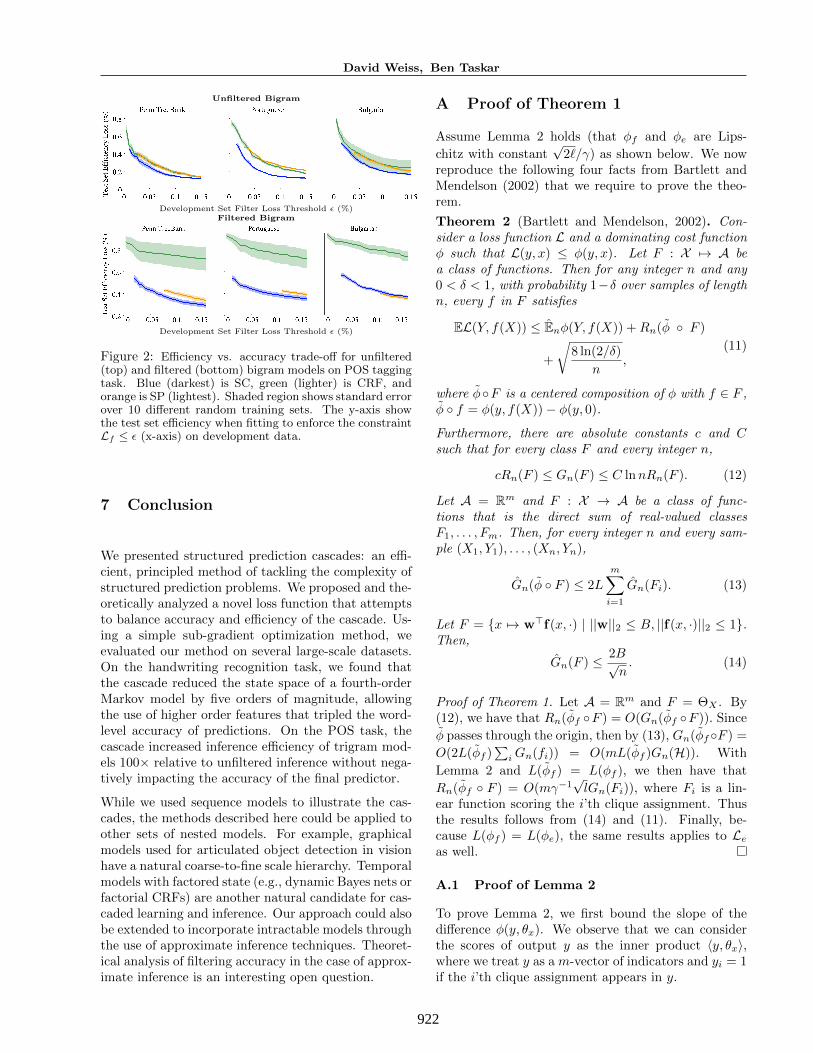
We next investigated the efficiency vs. filtering accu-racy trade-off of SC compared to the SP and CRFbaselines on all three languages. For each of thethree languages, we generated 10 different trainingsets from 40% of the full training datasets. Random-ization was taken with the same 10 seeds for eachdataset/algorithm pair. For all methods, we trainedbigram models under two conditions: first, as the ini-tial step of a cascade (e.g., no prior filtering), and sec-ond, as the second step of a cascade after initial filter-ing by the SC algorithm with ε = 0.05%, and analyzedthe resulting trade-off between efficiency and accuracy.

The results are presented in Figure 2. The figures weregenerated by computing for each ε along the x-axis thecorresponding test efficiency Le when the constraint onfilter loss (Lf ≤ ε) is enforced using development setdata. Points for which the constraint could not be en-forced (even with α = 0) are not shown. SC handilybeats the competitors in both the filtered and unfil-tered case. Note that in the unfiltered condition, theCRF is unable to achieve significant pruning efficiencyfor any ε, while the SP cannot achieve filtering accu-racy for small ε. However, because SC and SP becomeequivalent as α approaches 1, we observe that the per-formance of SC and SP converge as ε increases.

922


Unfiltered Bigram

Development Set Filter Loss Threshold ε (%)Filtered Bigram

Development Set Filter Loss Threshold ε (%)

Figure 2: Efficiency vs. accuracy trade-off for unfiltered(top) and filtered (bottom) bigram models on POS taggingtask. Blue (darkest) is SC, green (lighter) is CRF, andorange is SP (lightest). Shaded region shows standard errorover 10 different random training sets. The y-axis showthe test set efficiency when fitting to enforce the constraintLf ≤ ε (x-axis) on development data.

7 Conclusion

We presented structured prediction cascades: an effi-cient, principled method of tackling the complexity ofstructured prediction problems. We proposed and the-oretically analyzed a novel loss function that attemptsto balance accuracy and efficiency of the cascade. Us-ing a simple sub-gradient optimization method, weevaluated our method on several large-scale datasets.On the handwriting recognition task, we found thatthe cascade reduced the state space of a fourth-orderMarkov model by five orders of magnitude, allowingthe use of higher order features that tripled the word-level accuracy of predictions. On the POS task, thecascade increased inference efficiency of trigram mod-els 100× relative to unfiltered inference without nega-tively impacting the accuracy of the final predictor.

While we used sequence models to illustrate the cas-cades, the methods described here could be applied toother sets of nested models. For example, graphicalmodels used for articulated object detection in visionhave a natural coarse-to-fine scale hierarchy. Temporalmodels with factored state (e.g., dynamic Bayes nets orfactorial CRFs) are another natural candidate for cas-caded learning and inference. Our approach could alsobe extended to incorporate intractable models throughthe use of approximate inference techniques. Theoret-ical analysis of filtering accuracy in the case of approx-imate inference is an interesting open question.

A Proof of Theorem 1

Assume Lemma 2 holds (that φf and φe are Lips-

chitz with constant√

2`/γ) as shown below. We nowreproduce the following four facts from Bartlett andMendelson (2002) that we require to prove the theo-rem.

Theorem 2 (Bartlett and Mendelson, 2002). Con-sider a loss function L and a dominating cost functionφ such that L(y, x) ≤ φ(y, x). Let F : X 7→ A bea class of functions. Then for any integer n and any0 < δ < 1, with probability 1−δ over samples of lengthn, every f in F satisfies

EL(Y, f(X)) ≤ Enφ(Y, f(X)) +Rn(φ ◦ F )

+

√8 ln(2/δ)

n,

(11)

where φ◦F is a centered composition of φ with f ∈ F ,φ ◦ f = φ(y, f(X))− φ(y, 0).

Furthermore, there are absolute constants c and Csuch that for every class F and every integer n,

cRn(F ) ≤ Gn(F ) ≤ C lnnRn(F ). (12)

Let A = Rm and F : X → A be a class of func-tions that is the direct sum of real-valued classesF1, . . . , Fm. Then, for every integer n and every sam-ple (X1, Y1), . . . , (Xn, Yn),

Gn(φ ◦ F ) ≤ 2L

m∑i=1

Gn(Fi). (13)

Let F = {x 7→ w>f(x, ·) | ||w||2 ≤ B, ||f(x, ·)||2 ≤ 1}.Then,

Gn(F ) ≤ 2B√n. (14)

Proof of Theorem 1. Let A = Rm and F = ΘX . By(12), we have that Rn(φf ◦F ) = O(Gn(φf ◦F )). Since

φ passes through the origin, then by (13), Gn(φf ◦F ) =

O(2L(φf )∑iGn(fi)) = O(mL(φf )Gn(H)). With

Lemma 2 and L(φf ) = L(φf ), we then have that

Rn(φf ◦ F ) = O(mγ−1√lGn(Fi)), where Fi is a lin-

ear function scoring the i’th clique assignment. Thusthe results follows from (14) and (11). Finally, be-cause L(φf ) = L(φe), the same results applies to Leas well.

A.1 Proof of Lemma 2

To prove Lemma 2, we first bound the slope of thedifference φ(y, θx). We observe that we can considerthe scores of output y as the inner product 〈y, θx〉,where we treat y as a m-vector of indicators and yi = 1if the i’th clique assignment appears in y.

923


Lemma 3. Let f(θx) = 〈y, θx〉 −maxy′ 〈y′, θx〉. Then

f(u)− f(v) ≤√

2`||u− v||2.

Proof. Let yu = argmaxy′ 〈y′, u〉 and yv =argmaxy′ 〈y′, v〉. Then we have,

f(u)− f(v) = 〈y, u〉 − 〈yu, u〉+ 〈yv, v〉 − 〈y, v〉= 〈yv − y, v〉+ 〈y − uu, u〉+ 〈yv, u〉 − 〈yv, u〉= 〈yv − y, v − u〉+ 〈u, yv − yu〉≤ 〈yv − y, v − u〉

≤ ||yv − y||2||u− v||2 ≤√

2`||u− v||2.

The last two steps follow from the fact that yu maxi-mizes 〈yu, u〉 (so 〈u, yv − yu〉 is negative), applicationof Cauchy-Schwarz, and from the fact that there areat most ` cliques appear, each of which can contributea single non-zero entry in y or yv.

Lemma 4. Let f ′(θx) = 〈y, θx〉 −1m

∑c∈C,yc maxy′:y′c=yc 〈y

′, θx〉. Then f(u) − f(v) ≤√2`||u− v||2.

Proof. Let yui = argmaxy′:y′c=yc 〈y′, u〉 for the i’th

clique assignment yc, and yvi the same for v. Thenwe have,

f ′(u)− f ′(v) =1

m

m∑i=1

〈y, u〉 − 〈yui, u〉+ 〈yvi, v〉 − 〈y, v〉

≤ 1

m

m∑i=1

〈yvi − y, v − u〉

≤ 1

m

m∑i=1

√2`||u− v||2 =

√2`||u− v||2.

Here we have condensed the same argument used toprove the previous lemma.

Lemma 5. Let g(θx) = 〈y, θx〉 − tx(α). Then g(u) −g(v) ≤

√2`||u− v||2.

Proof. Plugging in the definition of tx(α), we see thatg(θx) = αf(θx)+(1−α)f ′(θx). Therefore from the pre-vious two lemmas we have that g(u)−g(v) = α(f(u)−f(v)) + (1− α)(f ′(u)− f ′(v)) ≤

√2`||u− v||2.

From Lemma 5, we see that φ(y, ·) = g(·) is Lip-schitz with constant

√2`. We can now show that

φf and φe are Lipschitz continuous with constant√2`/γ. Let L(·) denote the Lipschitz constant. Then

L(φt) = L(rγ) · L(φ(y, ·)) ≤√

2`/γ.

To show L(φe) requires more bookkeeping becausewe must bound φ(y?(yc), θx). We can prove equiva-lent lemmas to lemmas 3, 4 and 5 where we substi-tute 〈y, θx〉 with maxy′:y′c=yc 〈y

′, θx〉, and thus show

that L(φ(y?(yc), ·)) ≤√

2`. Therefore, L(φe) =1m

∑c∈C,yc L(rγ) · L(φ(y?(yc), ·)) ≤

√2`/γ, as desired.

References

S. Afonso, E. Bick, R. Haber, and D. Santos. FlorestaSinta(c)tica: a treebank for Portuguese. In Proc. LREC,2002.

Y. Altun, I. Tsochantaridis, and T. Hofmann. HiddenMarkov support vector machines. In Proc. ICML, 2003.

P. L. Bartlett and S. Mendelson. Rademacher and Gaus-sian complexities: Risk bounds and structural results.Journal of Machine Learning Research, 3:463–482, 2002.

X. Carreras, M. Collins, and T. Koo. TAG, dynamic pro-gramming, and the perceptron for efficient, feature-richparsing. In Proc. CoNLL, 2008.

E. Charniak. A maximum-entropy-inspired parser. In Proc.NAACL, 2000.

M. Collins. Discriminative training methods for hiddenmarkov models: theory and experiments with percep-tron algorithms. In Proc. EMNLP, 2002.

G. Druck, M. A. Amherst, M. Narasimhan, W. A. Red-mond, and P. Viola. Learning A* underestimates: Usinginference to guide inference. In Proc. AISTATS, 2007.

R. Kassel. A Comparison of Approaches to On-lineHandwritten Character Recognition. PhD thesis, Mas-sachusetts Institute of Technology, 1995.

J. Lafferty, A. McCallum, and F. Pereira. Conditional ran-dom fields: Probabilistic models for segmenting and la-beling sequence data. In Proc. ICML, 2001.

M. Marcus, S. Santorini, and M. Marcinkiewicz. Buildinga large annotated corpus of english: the penn treebank.Computational Linguistics, 19(2):313–330, 1993.

C. Pal, C. Sutton, and A. McCallum. Sparse forward-backward using minimum divergence beams for fasttraining of CRFs. In Proc. ICASP, 2006.

S. Petrov. Coarse-to-Fine Natural Language Processing.PhD thesis, University of California at Bekeley, 2009.

A. Ratnaparkhi. A maximum entropy model for part-of-speech tagging. In Proc. EMNLP, 1996.

S. Shalev-Shwartz, Y. Singer, and N. Srebro. Pegasos: Pri-mal estimated sub-gradient SOlver for SVM. In Proc.ICML, 2007.

K. Simov, P. Osenova, M. Slavcheva, S. Kolkovska, E. Bal-abanova, D. Doikoff, K. Ivanova, A. Simov, E. Simov,and M. Kouylekov. Building a linguistically interpretedcorpus of bulgarian: the bultreebank. In Proc. LREC,2002.

B. Taskar, C. Guestrin, and D. Koller. Max margin Markovnetworks. In Proc. NIPS, 2003.

P. Viola and M. Jones. Robust real-time object detection.International Journal of Computer Vision, 57(2):137–154, 2002.

structured prediction cascades

Documents