Structured Products and the Mischief of Self-Indexing

by

Geng Deng, PhD, CFA, FRM,

Craig McCann, PhD, CFA,

and Mike Yan, PhD, CFA, FRM 1

1. INTRODUCTION

In recent years, investment banks have issued structured products linked to indexes they

create rather than just linking to standardized indexes from Standard & Poor’s. In doing so, the

investment banks created additional difficulties for investors evaluating these investments. We

illustrate the potential conflicts of interest investment banks created by linking their structured

products to proprietary volatility indexes although the conflicts are present in other proprietary

index-based investments as well.

In the late 1980s and early 1990s, equity-linked notes were issued by operating

companies in financial distress. These mandatory convertible securities, branded PERCS,

PRIDES, DECS, ACES, PEPS etc., provided rating agency equity capital and preserved

deductibility of interest payments. For example, in 1992, Citicorp issued $1 billion of 3-year

Preferred Equity Redemption Cumulative Stock (PERCS) issued at a time when Citicorp had

suspended its dividend and its stock price had declined from over $30 to under $15 in the prior

two years. 2 At maturity, Citicorp paid the lesser of the value of one share of Citicorp stock and

$20.28. Setting aside the PERCS’ $0.30425 quarterly dividend and the expected Citicorp

dividend, this payoff is the same as purchasing Citicorp at its current $14.75 market value and

selling a 3-year out-of-the-money call option with a $20.28 strike price. This Citicorp PERCS is

very similar to what later became known as reverse convertibles.

In 1994, Reynolds Metals issued $472.5 million 4-year Preferred Redeemable Increased

Dividend Equity Securities (PRIDES).3 At maturity, Reynolds Metals paid the lesser of the value

1 © Securities Litigation and Consulting Group, Inc, 2016. Geng Deng can be reached at 703-760-6180 or

at GengDeng@gmail.com. Craig McCann can be reached at 703-246-9381 or at

CraigMcCann@slcg.com. Mike Yan can be reached at 703-539-6780 or MikeYan@slcg.com.

2 This offering pre-dates SEC's Edgar system. A copy of the prospectus is available at

www.slcg.com/OtherStructuredProductResearch/Citicorp%201992%20PERCS%20Prospectus.pdf.

3 This issue occurred in January 1994 just as Edgar launched and the offering document is available here

www.sec.gov/Archives/edgar/data/83604/0000083604-94-000007.txt.

2

© Securities Litigation and Consulting Group, Inc.

of one share of Reynolds stock and $47.25 plus 82% of any excess above $57.62. This maturity

payoff could be achieved by purchasing Reynolds’ stock at its then current $47.25 market value,

selling a 4-year at-the-money call option and buying 0.82 call options with a $57.62 strike price.

The Reynolds Metals' PRIDES are very similar to what later became known as tracking

securities under brand names such as Performance Leveraged Upside Securities or PLUS.

Early equity-linked notes were also used by corporations and wealthy investors to

“monetize” highly appreciated stock positions, shedding risk and deferring taxes. For example,

in 1996 Times Mirror issued $51.2 million of Premium Equity Participating Securities (PEPS)

linked to the price of Netscape.4 Times Mirror had acquired pre-IPO Netscape shares and seen

the value post-IPO Netscape shares skyrocket and start to fall back to earth. At maturity, Times

Mirror paid the value of a share of one share of Netscape stock if less than $39.25 or $39.25 plus

87% of any excess above $45.14. Times Mirror deferred taxes for 5 years, shed the downside

risk in Netscape, kept the first 15% upside, and 15% of any further gains.

Later in the 1990s, investment banks switched from underwriting reverse convertibles

and tracking securities issued by operating companies like Citicorp and Reynolds Metals linked

to their own stock to issuing and underwriting structured products linked to unrelated publicly

traded companies. This change in investment banks' role led to a dramatic proliferation of new

structured product issuances and ever more complicated payoff structures since the investment

banks were no longer limited to underwriting securities other companies wanted to issue.

Investment banks could now issue notes in small denominations linked to publicly traded

companies that affiliated brokerage firms could then sell through their retail sales forces.

Lehman Brothers’ 1998 $1 million Yield Enhanced Equity Linked Debt Security

(YEELDS) is an early reverse convertible issued by an investment bank linked to an unrelated

publicly traded company.5 At maturity, Lehman paid the lesser of the value of one share of Cisco

Systems’ stock and $100.75. Setting aside the YEELDS’ $0.83 quarterly dividend and the

expected Cisco Systems’ dividend, this payoff was similar to purchasing Cisco Systems at

$66.50 and selling a 3-year call option with a $100.75 strike price.

4 The offering circular is available here www.sec.gov/Archives/edgar/data/925260/0000950150-96-

000146.txt.

See also Floyd Norris, “Times Mirror to Cash In on Netscape's Rise” New York Times, March 5, 1996.

http://www.nytimes.com/1996/03/05/business/times-mirror-to-cash-in-on-netscape-s-rise.html

5 www.sec.gov/Archives/edgar/data/806085/0001047469-98-008488.txt

Preliminary Draft

3

Deng, McCann and Yan

Structured Products and the Mischief of Self-Indexing

Investment banks acting as issuers as well as underwriters created ever more complex

payoff structures late last decade. Capped and leveraged dual directional and autocallable

structured products are examples of payoff structures grown so complicated that they lost readily

apparent investment meaning.6 The complexity of these notes made regulatory oversight more

difficult and allowed investment banks to sell structured products with very low issue date

values. Since April 2012, the SEC partially ameliorated the problem of low-value structured

products by requiring prominent disclosure of issue date fair values.7

As part of their evolution, investment banks became index providers as well as

underwriters and issuers of structured products late last decade. Rather than using indexes from

Standard and Poor’s and other independent index providers, investment banks began to “self-

index”. As we show in what follows, issuing and underwriting structured products linked to

proprietary indexes has led investment banks to mischief. Costs which had previously been built

into payoff structures based on indexes which did not contain trading costs or disclosed as annual

deductions from third party index returns were now being built into the index construction where

they were much harder for investors and regulators to identify and quantify. We illustrate the

problems with self-indexing structured products with proprietary volatility indexes from Bank of

America and JP Morgan.

In the past year, regulators have brought enforcement actions related to structured

products linked to proprietary indexes. In October 2015, the Securities and Exchange

Commission (“SEC) settled charges against UBS over its V10 Currency Index finding that UBS

did not disclose that it was applying bid-ask spread trading costs when rebalancing the currencies

in its proprietary index. 8 In June 2016, the SEC and FINRA reached settlements with Merrill

Lynch over structured products linked to Bank of America’s proprietary VOL Index finding that

6 See for example Credit Suisse's 2012 Absolute Return Barrier Securities at

www.sec.gov/Archives/edgar/data/1053092/000095010312004245/dp32342_424b2-u696.htm. 7 https://www.sec.gov/divisions/corpfin/guidance/structurednote0412.htm. 8 The SEC press release announcing the UBS V10 Currency Index settlement is available at

www.sec.gov/news/pressrelease/2015-238.html and its Order Instituting Proceedings is available at

https://www.sec.gov/litigation/admin/2015/33-9961.pdf.

4

© Securities Litigation and Consulting Group, Inc.

hypothetical trading costs in the calculation of the VOL Index returns and therefore the returns

on the linked structured products was inadequately disclosed.9

2. VIX FUTURES, INDEXES AND STRUCTURED PRODUCTS

The Chicago Board Options Exchange (CBOE) first published the Volatility Index (VIX)

in the early 1990s and, in 2003, reformulated it as a weighted average of S&P 500 options prices

across a range of strike prices and with between 9 and 60 days to expiration.10 In 2014, the

CBOE began using SPX WeeklysSM options to narrow the range of option expirations used in the

calculation of the VIX to between 23 and 37 days.

The correlation between weekly changes in the VIX and weekly changes in the S&P 500

over the period from January 1, 1990 to June 30, 2016 was -0.72. The negative correlation has

led some to argue that investors could hedge stock portfolios with VIX-related derivatives.11

Since the VIX itself is simply a calculated index value and is not directly investable, investors

gain exposure to the VIX, and therefore any potential hedging benefit, through derivatives

contracts (i.e. futures and options) whose payoffs depend on future realized values of the VIX.

The CBOE began trading future contracts based on the VIX on March 26, 2004. The

CBOE maintains a set of futures contracts on the VIX expiring each month for the next nine

months plus five contracts expiring quarterly in February, May, August and November spanning

up to 15 months in the future. VIX futures contracts settle on a Wednesday thirty days prior to

the third Friday of the following month. The contract closest to expiration is referred to as the

first-month contract, and later expiring contracts in sequence are second-month contract, third-

month contract and so on. VIX futures prices typically increase with the remaining time to

expiration. That is, it is common for contract prices to drop over time as they mature unless the

whole term structure is shifting up.

The S&P 500 VIX Short-Term Futures Total Returns Index (SPVXSTR) reflects the

daily returns to a fully collateralized long position in short term VIX futures contracts with

interest accrual based on 91-day US Treasury rate. The daily return of the index is based on the

9 The SEC press release announcing the Bank of America VOL Index settlement is available at

www.sec.gov/news/pressrelease/2016-129.html and its Order Instituting Proceedings is available at

www.sec.gov/litigation/admin/2016/33-10103.pdf. The companion FINRA settlement press release is

available at www.finra.org/newsroom/2016/finra-fines-merrill-lynch-5-million-related-return-notes-sales

and AWC is available at www.finra.org/sites/default/files/Merrill_AWC_062316.pdf.

10 See Carr and Wu (2006) for an explanation of the old and new VIX calculations. 11 See Deng, McCann and Wang (2012) for a discussion of VIX ETPs as a hedge for stock portfolios.

Preliminary Draft

5

Deng, McCann and Yan

Structured Products and the Mischief of Self-Indexing

weighted average returns of the first-month and the second-month VIX futures contract. The

weights on the two contracts are adjusted daily such that the weighted maturity of the included

contracts is one month. Throughout each roll-over period, first-month VIX futures contracts are

gradually replaced by second-month VIX futures contracts. At the end of a roll period, all the

weight applied to calculate that day’s return is on the second-month contract which then becomes

the first-month contract and the third-month contract becomes the second-month contract for the

next roll period.12

Similarly, the S&P 500 VIX Mid-Term Futures Total Returns Index (SPVXMTR) uses a

weighted average of fourth-, fifth-, sixth- and seventh-month VIX futures contracts to estimate

the returns to a fully collateralized long position in a VIX futures contract expiring in five

months. Every day the index rolls over some of the weight from the fourth-month contract into

the seventh-month contract while keeping the weights on the fifth-month and sixth-month

contracts constant. Like the SPVXSTR, the SPVXMTR includes interest accrual based on the

91-day US Treasury rate.

In addition to the short-term and medium-term total return indices, S&P publishes the

S&P 500 VIX Short-Term Futures Index Excess Return, or SPVXSP, and the S&P 500 VIX

Mid-Term Futures Index Excess Return, SPVXMP, which exclude the Treasury interest that

would accrue on a fully collateralized futures position.

Exchange traded products (ETPs) have been issued on both the total return and excess

return versions of S&P’s VIX Short Term and Mid-Term Futures Indexes. Shortly after S&P

published the S&P 500 VIX Short-term Future Index and Mid-term Future Index on January 22,

2009, Barclays issued two exchange traded notes (ETNs), VXX linked to S&P 500 VIX Short-

Term Futures Index and VXZ linked to S&P 500 VIX Mid-Term Futures Index, that each had a

face value of $250 million. By June 2016, Barclays had raised gross proceeds of $11.9 billion

from issuing VXX ETNs and $1.8 billion from issuing VXZ ETNs. As of June 30, 2016,

Barclays has raised gross proceeds of $15.65 billion from issuing various ETNs linked to S&P

500 VIX Futures Indices, including leveraged and inverse ETNs.

12 For more details see, S&P VIX Futures Indices, Methodology, March 2016. http://us.spindices.com/documents/methodologies/methodology-sp-vix-future-index.pdf

6

© Securities Litigation and Consulting Group, Inc.

In January 2011, ProShares issued the ProShares VIX Short-Term Futures ETF (VIXY)

which tracks the S&P VIX Short-Term Futures Index and the ProShares VIX Mid-Term Futures

(VIXM) which tracks the S&P Mid-Term VIX Futures Index. In October 2011, ProShares issued

SVXY which is an inverse ETF and UVXY which is a twice-leveraged inverse ETF based on the

S&P VIX Short-Term Futures Index. As of December 31, 2015, those four ETFs had a market

exposure of roughly $1.15 billion.13 In November 2011, VelocityShares and UBS issued VIX-

related long-term ETNs. VelocityShares issued 20-year ETNs based on the S&P VIX Futures

Indices, and UBS issued 30-year ETNs based on the S&P VIX Futures Indices.

S&P’s VIX Futures Indices allow issuers to design ETPs with returns focused on at least

six different dates on the VIX futures term structure plus several complicated combinations of

positions on the term structure. Rather than linking structured products to the S&P VIX Futures

Indices, Bank of America and JP Morgan published and used their own “proprietary” volatility

indexes which are ultimately derived from the same set of S&P Index options or VIX futures

contracts as are the S&P VIX Futures Indices.14

3. BANK OF AMERICA’S PROPRIETARY INDEX AND STRUCTURED PRODUCTS

Bank of America describes its VOL Index as an investable benchmark “designed to

measure the return of an investment in the forward implied volatility of the S&P 500® Index.”

The VOL Index tracks the 3-month implied volatility of the S&P 500 index three and a half

months forward, i.e. for the period from 3.5 months to 6.5 months in the future. Bank of America

first published the VOL Index on March 23, 2010, back-filling the index to a starting index level

of 250 on December 31, 2004.

13 www.sec.gov/Archives/edgar/data/1415311/000119312516485710/d92789d10k.htm. 14 Citigroup’s Citi Volatility Index Total Return (“CVOLT”) Index is a more complicated

combination of twice-leveraged third-month and fourth-month futures contracts and a short position in the

S&P 500. The size of the short position is determined by regression analysis to maximize the correlation

between the VIX and the CVOLT. Like the S&P Total Return VIX Futures Indexes, the CVOLT Index

level includes interest accruing at the 91day Treasury bill rate. Citigroup calculated the CVOLT Index

starting in October 2010 and backfilled the index to 2005. Citigroup issues C-Tracks 10-year ETNs linked

to the CVOLT Index in November 2010, and increased its issuance in 2012, 2013, and 2014. In total

Citigroup received gross proceeds of $132.6 million from issuing CVOLT ETNs.

Deutsche Bank’s ELVIS index measures the returns to a strategy of investing in forward starting

6-month variance swaps. There do not appear to be any retail structured products or ETNs linked solely to

the ELVIS or ELVIS II indexes. Deutsche Bank issued several structured products linked to a basket of

indexes, which included its ELVIS II Index as one basket component. The weights of the ELVIS II Index

in the baskets was always 13% or less.

Preliminary Draft

7

Deng, McCann and Yan

Structured Products and the Mischief of Self-Indexing

The VOL Index is not calculated from VIX futures contracts like the S&P VIX Futures

Indices but instead from four CBOE spot VIX calculations based on S&P 500 Index option

contracts expiring in March, June, September, and December denoted as VXMAR, VXJUN,

VXSEP, and VXDEC. The CBOE calculates VXMAR, VXJUN, VXSEP, and VXDEC in a

similar manner to the VIX calculation although the CBOE’s weighting of option prices of

different expirations in its calculation of the VIX is unnecessary since VXMAR is based only on

the prices of S&P options all expiring on the same day in March, VXJUN is based only on the

prices of S&P options all expiring on the same day in June, and so on.

In general, a forward implied volatility between two dates in the future, t1 and t2 can be

calculated as follows.

𝐹𝑜𝑟𝑤𝑎𝑟𝑑 𝐼𝑚𝑝𝑙𝑖𝑒𝑑 𝑉𝑜𝑙𝑎𝑡𝑖𝑙𝑖𝑡𝑦𝑡1𝑡𝑜 𝑡2= √

𝐼𝑚𝑝𝑙𝑖𝑒𝑑 𝑉𝑜𝑙𝑎𝑡𝑖𝑙𝑖𝑡𝑦𝑡𝑜 𝑡2

2𝑡2 − 𝐼𝑚𝑝𝑙𝑖𝑒𝑑 𝑉𝑜𝑙𝑎𝑡𝑖𝑙𝑖𝑡𝑦𝑡𝑜 𝑡1

2𝑡1

𝑡2 − 𝑡1

For example, we can estimate 3-month implied volatility four months in the future from implied

volatilities based on market prices of options expiring in seven months (t1 = 7 months) and from

implied volatilities based on market prices of options expiring in four months (t1 = 4 months).

Following Bank of America’s notation, we refer to VXMAR, VXJUN, VXSEP, and

VXDEC as Index Components. The nearest Index Component is denoted IC1; second-, third-

and fourth-to-nearest Index Components are referred to as IC2, IC3, and IC4, respectively. These

Index Components are not forward contract prices. They are approximate implied volatilities

covering the periods from the current date to expiration dates of S&P 500 Index options in

March, June, September and December. IC1, IC2, IC3, and IC4 are used to estimate the quarterly

Forward Implied Volatility (“FIV”) between adjacent Index Components.

The nearest FIV, denoted as FIVA, is the implied volatility starting from the nearest to

expiration of the four Index Components, IC1, to the second-to-nearest to expiration, IC2.

Similarly, FIVB and FIVC are the forward implied volatilities starting from the second Index

Component, IC2, expiration to the third Index Component, IC3, expiration, and from the third

Index Component, IC3, expiration to the fourth Index Component, IC4, expiration.

𝐹𝐼𝑉𝐴 = √𝐼𝐶22𝑡2−𝐼𝐶12𝑡1

𝑡2−𝑡1, 𝐹𝐼𝑉𝐵 = √

𝐼𝐶32𝑡3−𝐼𝐶22𝑡2

𝑡3−𝑡2, 𝐹𝐼𝑉𝐶 = √

𝐼𝐶42𝑡4−𝐼𝐶32𝑡3

𝑡4−𝑡3

8

© Securities Litigation and Consulting Group, Inc.

Since the VOL Index is to measure changes in the 3-month forward implied volatility

centered five months in the future, the calculation agent uses FIVA and FIVB which are centered

before and after five months in the future. Denote the FIV that is centered right before the 5-

month point as FIV1, and the FIV that is centered after as FIV2.

The FIV1 and FIV2 values fluctuate every day, reflecting the changing levels of the

Index Components (VXMAR, VXJUN, VXSEP and VXDEC). The center of the date range

covered by VOL remains 5 months in the future so, as time passes, if the Index Components’

values don’t change much from one day to the next, the weight on FIV1 is steadily reduced to

0% and the weight on FIV2 is steadily increased to 100%. When the weight on FIV1 drops to

0% and the weight on FIV2 has increased to 100%, the old FIV2 becomes the new FIV1 with a

weight of 100% and the old FIV3 becomes the new FIV2 with a weight of 0% and the rolling

from FIV1 to FIV2 starts again.

The daily return of the synthetic portfolio equals the weighted change in the FIV1 and

FIV2 values less the impact of an “Execution Factor”. Setting aside the Execution Factor, the

value of the synthetic portfolio is equivalent to investing $100 split between the two forward

implied volatility contracts, FIV1 and FIV2, with weights rebalanced daily. For example, if the

weights are 40% and 60% for FIV1 and FIV2, respectively, then $40 is invested in FIV1 and $60

is invested in FIV2. On the next day, the portfolio becomes more or less valuable depending on

changes in the value of the $40 invested in FIV1 and the $60 invested in FIV2. At the end of

each day, the synthetic portfolio is rebalanced to reflect the newly calculated portfolio weights

which change because of the passage of time. In addition, because of daily changes in the

relative value of FIV1 and FIV2 the number of units of FIV1 and FIV2 contracts which should

be held to establish the desired portfolio weights changes daily.

Assume the hypothetical portfolio value increases from $100 to $105 because the spot

VIX term structure has become steeper, and the updated FIV weights become 38% and 62%.

Then the target value of FIV1 is $39.90 (i.e. 38% of $105), and the target value of FIV2 is

$65.10. There is no chance the portfolio starts the second day with $39.90 in FIV1 and $65.10 in

FIV2, and thus would not require any rebalancing. Instead, each day the portfolio is rebalanced

to reflect the new weights, i.e., some units of one of the hypothetical contracts are sold and units

of the other contract are purchased.

Preliminary Draft

9

Deng, McCann and Yan

Structured Products and the Mischief of Self-Indexing

In our example, if the increase in the portfolio value is solely due to an increase of the

$40 invested in FIV1 to $45, with FIV2 unchanged, then $5.1 of FIV1 must be sold, and the

proceeds used to purchase FIV2. The proceeds - $5.1 in our example - are subject to the

Execution Factor, and the purchased FIV2 amount is reduced to $5.025, the ratio of the proceeds

and the Execution Factor (i.e., $5.1/1.015). Thus at the end of the day, instead of the hypothetical

portfolio being worth $105, it is only worth 104.925, equivalent to a seven basis point (0.07%)

daily charge.

Because the Execution Factor is applied to hypothetical contracts purchased each day as

part of the rebalancing, the daily cost fluctuates from zero in the vanishingly rare instances when

no rebalancing occurs to significantly more than seven basis points when the rebalancing

required exceeds the average daily rebalancing. While the impact of the Execution Factor on any

individual day is variable and uncertain, the impact over the five-year term of Bank of America’s

structured products is fixed and certain. Every quarter the entire portfolio value is eventually

transferred from the FIV1 contract to the FIV2 contract and the entire unencumbered index value

is subjected to the Execution Factor four times a year. Thus, the Execution Factor embeds a

phantom transaction cost of 6% per year into the construction of the VOL Index.

The daily return of the synthetic portfolio is multiplied by a 120% “Index Multiplier” and

then increased by the 30-day Treasury-bill rate to determine the daily return of the VOL Index.

The Index Multiplier magnifies the impact of the Execution Factor by 20% so the trading costs

Bank of America incorporates into the volatility index calculation is 7.20% per year.

The impact on investors of Bank of America deducting 7.2% daily from the

unencumbered index through the Execution Factor and then 0.75% through the Index Fee is the

same as deducting 7.9% at the structured product level from an index calculated without the

embedded phantom trading costs. 15 To demonstrate that Bank of America was deducting 7.9%

per year from the levels implied by changes in forward implied volatility we assume that instead

of applying an Execution Factor, Bank of America deducted a 7.2% annual index charge daily

from the thus unencumbered VOL Index. We first calculate the daily return of the VOL Index

without the Execution Factor, then reduce these daily returns by 7.2% divided by 252 days.

15 7.9% = 1 - (1-7.2%)*(1-0.75%).

10

© Securities Litigation and Consulting Group, Inc.

In Figure 1, we plot the impact of the Execution Factor against the impact of a 7.2%

annualized deduction from the index and draw a regression line through the data. The vertical

axis measures the impact of the Execution Factor on the change in the VOL Index level over

rolling 12 month windows. The horizontal axis measures the impact of alternatively applying a

7.2% annual charge daily on the change in the VOL Index level over the same rolling 12 month

windows. The effective annual cost of the Execution Factor and the 7.2% fixed fee are highly

correlated with an R-squared value 0.9995. The complex method by which the Execution Factor

is included in the index calculation has no economic substance other than to add an additional

7.2% annual deduction from the unencumbered index at the structured product level.

Figure 1: Execution Factor and 7.2% Annual Charge Have Identical Impacts.

Further, in Figure 2 we plot the VOL Index and the VOL Index without the Execution

Factor but with a fixed annual fee of 7.2%. The difference between the VOL Index and the

replicated VOL Index using a 7.2% annualized fee deducted daily is trivial. As of June 30, 2016,

the VOL Index level is 8.97, and the index level with 7.2% fee is 9.77 – 0.8 or 0.3% of the

starting value after 12 years of daily calculations.

y = 1.0322x - 0.0026R² = 0.9989

0%

5%

10%

15%

20%

0% 5% 10% 15% 20%

Imp

act

of

Exe

cuti

on

Fac

tor

Impact of Annual Fee of 7.2%

Preliminary Draft

11

Deng, McCann and Yan

Structured Products and the Mischief of Self-Indexing

Figure 2: Levels of the VOL Index with and without the Execution Factor, and the

Modified Index with a 7.2 % Annual Fee

The correlation between weekly changes in the VOL Index and changes in the S&P 500

VIX Mid-Term Futures Total Return Index, which is based on the prices of fourth, fifth, sixth

and seventh-month futures contracts on the VIX, between December 2005 and June 2016 is 0.90.

That means 81% of the variation in the VOL Index can be explained by the variation in the S&P

500 VIX Mid-Term Futures. Informed investors who wanted whatever exposure a VOL-linked

structured product could provide would instead purchase Barclays’ VXZ ETNs or some other

S&P Mid-Term VIX Futures Index based investment.

By embedding costs in the index construction, Bank of America was able to lower the

amounts it would have to pay out to purchasers of its structured products. Standard and Poor’s

does not incorporate any estimated transaction costs in its calculation of the S&P VIX Futures

Indices referenced by other firms’ ETPs. These other ETP issuers disclose an annual deduction

from the S&P VIX futures indexes of 0.85% and 0.89%, significantly lower than the undisclosed

but quantifiable and certain annual costs embedded in the VOL Index and charged 7.9% per year

at the structured product level.

0

100

200

300

400

500

600

700

VOL Index

7.2% Annual Charge

12

© Securities Litigation and Consulting Group, Inc.

4. JP MORGAN STRATEGIC VOLATILITY INDEX

Our second example of a proprietary index used to determine structured product payoffs

is JP Morgan’s Strategic Volatility (“Strat VOL”) Index. JP Morgan started calculating the Strat

VOL Index in July 2010 and backfilled it to September 2006.16 JP Morgan calculates the Index

from changes in the prices of an uncollateralized long position in the second-month and third-

month VIX futures contracts and contingent short position in the first-month and second-month

VIX futures contracts.

The return of a long position in second-month and third-month futures contracts and of

the short position in the first-month and second-month futures contracts are determined as flows.

1. Long Returnt = w1,t ×P2,t

P2,t−1+ w2,t ×

P3,t

P3,t−1− 1

2. Short Returnt = −1 × (w1,t ×P1,t

P1,t−1+ w2,t ×

P2,t

P2,t−1− 1)

where Pi,j is the price of the ith-month VIX futures contract on day j. The weights w1,t and w2,t

result in an approximate 60-day weighted maturity for the long futures positions and an

approximate 30-day weighted maturity for the short position when included in the index.

w1,t =Days Remaining in Current Period Between Rebalancing

Total Days in Current Period Between Rebalancing

w2,t = 1 − w2,t

The daily gross return of the Strat Vol Index on day t, before any fees is calculated as

3. Gross Returnt = 1 + Long Returnt − ℓt−1 × Short Returnt,

4. Return(t) = GrossReturn(t) − RebAdjAmount(t) − 0.75%∆t

5. Reblancing Adjustment Amount(t) = Rebalancing Adjustment Factor ×

(Daily Rebalancing Percentage (t)+ Short Exposure Change)

where ℓ𝑡−1 denotes the short exposure determined at the end of the previous day. The short

position is adjusted according to the shape of the VIX futures term structure. When the spot VIX

is below a weighted average of the first- and second-month VIX futures prices on each of the

16 JP Morgan also published the Strategic Volatility Dynamic Index, which is similar to the Strat VOL

Index but allocates weight to the third-, fourth-, fifth- and six-month contracts to center the long position

at 4 months in the future and allocates weight to the second- and third-month contracts to center the short

position at 2 months in the future. Our comment herein about the Strat Vol Index apply with only slight

modifications to the JP Morgan’s Strategic Volatility Dynamic Index.

Preliminary Draft

13

Deng, McCann and Yan

Structured Products and the Mischief of Self-Indexing

three immediately preceding business days (i.e., the VIX futures term structure is upward

sloping), the short exposure is increased 20% per day, up to 100%, to compensate for the

negative roll yield in the long position. When the spot VIX is above the weighted average of the

first- and second-month VIX futures prices on each of the preceding three business days (i.e., the

VIX futures term structure is downward sloping), the short exposure is decreased 20% per day,

down to 0%.

Up to this point the calculation and interpretation of the Strat Vol Index is pretty

straightforward. It is simply an estimate of the excess return to a long position in a rolling 2-

month VIX futures contract, supplemented by the return to a short 1-month VIX futures contract

when the VIX term structure is upward sloping.

JP Morgan could have calculated the Strat Vol Index based on the Gross Return above.

This is what Standard and Poor’s does in calculating the various VIX Futures Excess Return

Indices before adding 91-day Treasury yields to calculate its VIX Futures Total Return Indices.

Barclays and other investment banks issued ETPs linked to S&P’s VIX Futures Indices

deducting and disclosing any fees at the structured product level. In fact, the returns to the Strat

Vol can be closely replicated using two low cost, listed VIX ETPs.

To illustrate, consider a strategy of buying Barclays mid-term VIX futures ETN, VXZ,

and buying VelocityShares’ inverse short-term VIX futures ETN, XIV, whenever the VIX

futures term structure is upward sloping. We constructed a portfolio using the short exposure ℓ𝑡

indicator from the Strat VOL calculation to determine the weight on XIV. Our portfolio of VXZ

and VIX ETNs does not track the long exposure in JP Morgan’s Strat VOL Index perfectly

because VXZ is centered 4.5 months out on the VIX futures term structure while Strat Vol’s long

position is centered 2 months out on the term structure. Nonetheless, the dynamical trading

strategy we set up gives a correlation of 0.91 from the index inception to June 2016. However,

the annual cost on the ETNs, at 0.89% on VXZ and 1.35% on XIV, is significantly lower than

the greater than 10% annual costs JP Morgan embedded in its Strat Vol Index.

Similar to Bank of America’s application of the Execution Factor, JP Morgan clips the

Strat Vol Index returns each day through the application of its Adjustment Factor and

Rebalancing Adjustment Amount. The Adjustment Factor is a 0.75% per annum fee applied

daily. The Rebalancing Adjustment Amount is more complex but is never less than 4.8% per

14

© Securities Litigation and Consulting Group, Inc.

year and is almost always 9.6% per year. As we will see below, JP Morgan’s “estimated value”

for structured products linked to the Strat VOL Index notes is based on an index that only

includes the first term, the Gross Return, and excluded to two daily deductions from the index.

Since the JP Morgan structured notes payout at maturity exactly the change in the Strat

Vol Index over the term of the note, JP Morgan could apply the 0.75% fee at the structured

product level as Bank of America does with its 0.75% Index Adjustment Factor and as Barclays

does with the 0.85% annual fee applied to the S&P Mid-term Futures Index returns referenced by

the VXX ETN.

JP Morgan’s Rebalancing Adjustment Amount is substantially more complicated than the

Adjustment Factor. It includes an annual charge that is certain and a charge that varies with the

amount of short exposure and with the VIX level over time. It is the sum of the Daily

Rebalancing Percentage plus the Short Exposure Change together multiplied by the Rebalancing

Adjustment Factor.

The Daily Rebalance Percentage on any calculation date, is the sum of the absolute value

of changes in the weights on the three VIX future contracts, and the absolute changes of the short

exposure, |ℓ𝑡−1 − ℓ𝑡|. For example, if we assume there is 20 days in the rebalancing period,

then as the long position is rolled the weight on the third-month will increase daily by 5% and

the weight on the second-month will decrease daily by 5%. The absolute change in the weight

on each the third-month and the second-month contract is 5% for a total of 10%.

On days when the weight on the short position remains 0%, the Daily Rebalance

Percentage will be 10%. On days when the weight on the short position remains 100%, the daily

roll from the first-month contract to the second contract adds an additional 10% to the Daily

Percentage Rebalance for a total of 20%. When the short position remains 100%, daily changes

in the weight on the second-month contract in the short position exactly offset changes in the

weight on the second month contract in the long positon. Although JP Morgan’s calculation

assumes trading would equal 20% of the notional value of the contracts on such days, real world

trading would only equal 10% of the notional value of the contracts. Thus, an investor replicating

the Strat Vol strategy would trade much less than implied by the Daily Rebalancing Percentage.

In addition, on days when the weight on the short position is changing – whether

increasing or decreasing by 20% – the absolute value of the change in the short position

exposure, i.e. 20%, is added to the Daily Rebalance Percentage. JP Morgan appears to implement

Preliminary Draft

15

Deng, McCann and Yan

Structured Products and the Mischief of Self-Indexing

hypothetical trades twice on days when the weight in the short position changes after already

overstating the amount of trading necessary to adjust the long and short futures positions. Thus,

Daily Rebalancing Percentage significantly overstates the amount of trading required to

implement the Strat Vol strategy.

The VIX futures term structure is typically upward sloping. Table 1 reports the

percentage of days from index inception date of July 30, 2010 to June 30, 2016. 83.8% of the

time the weight on the contingent short position has been 100%. If we use the simplifying 20-day

roll period assumption and ignore the impact of changes in the short exposure which only

increases the Daily Rebalance Percentage, the average Daily Rebalance Percentage is 18.9%

based on the statistics in Table 1.

Table 1: Short Exposure is Significant and Unchanging.

Short Exposure Change in Exposure

0.00 0.20 0.40 0.60 0.80 1.00 -.20 0 +.20

Frequency 6.2% 1.7% 2.5% 2.5% 3.4% 83.8% 4.5% 91.0% 4.5%

The Daily Rebalancing Amount equals the Daily Rebalancing Percentage which can

range from 10% to 58% multiplied by the Rebalancing Adjustment Factor, R in Table 2. Using

0.2%, the lowest R, the Daily Rebalancing Amount is on average at least 0.038%, which is

equivalent to an annual fee of 9.54% across 252 trading days.

Table 2: Rebalancing Adjustment Factor by Daily VIX level and Frequency.

Day VIX Level Frequency R

≤ 35 97.9% 0.2%

≤ 50 and > 35 2.1% 0.3%

≤ 70 and > 50 0% 0.4%

> 70 0% 0.5%

The Daily Rebalancing Amount imparts a minimum annualized deduction on the Strat

Vol Index of 5%, even with the lowest R number, although it could be as high as 0.1% per day.

Back-testing the data from index inception to June 2016, we find that JP Morgan could replace

the Daily Rebalancing Amount by a 10.6% fixed annual deduction, similar to the 0.75% fixed

annual deduction JP Morgan subtracts from the index and the resulting index levels would be

within 1% of the levels derived by JP Morgan. On June 1, 2016, the JP Morgan index level is

158.57 and the index level with 10.6% fee is 159.61. As with the VOL Index, a simple fixed

16

© Securities Litigation and Consulting Group, Inc.

annual deduction from the Strat Vol Index would have had the same impact on the index and

therefore on investors as the convoluted application of the Daily Rebalancing Amount.

While Strat VOL Index is less complicated than VOL Index in that it is based on VIX

futures contracts instead of differences in implied volatilities from index options, JP Morgan’s

incorporation of trading costs into the index calculation through an Adjustment Factor is more

complicated and its impact more variable than Bank of America’s Execution Factor.

In Figure 3 we plot the Strat Vol Index as published by JP Morgan and our replication of

it assuming a 10.6% annual charge applied daily. We also plot the Strat Vol Index without the

Daily Rebalancing Amount deductions and the value of a portfolio of long positions in VXZ and

XIV which mimics the long and short exposure in the Strat Vol Index.

Figure 3: JP Morgan Strategic Volatility Index Levels, Replicated Index with Zero-

Rebalancing Fee, Daily Rebalanced Hedging Strategy, and Index with 10.6% Annual

Charge.

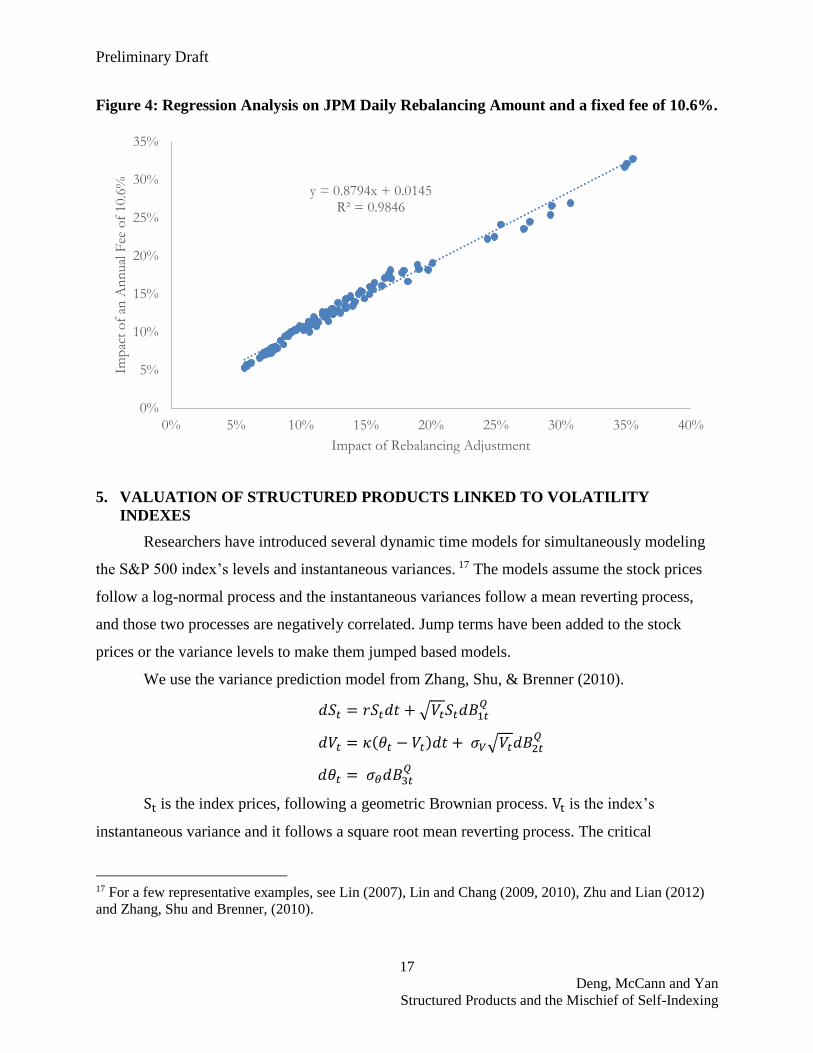
In Figure 4 we do the regression analysis on the annual impact of the Daily Rebalancing

Amount and the impact of a fixed charge of 10.6% per annum applied daily. The annual impact

from 2006 to 2016 has a very high correlation with R2 of 0.985

0

100

200

300

400

500

600

700

800

900

1000

JPM Index

Replicated Index Zero-Rebalancing Fee

Daily Rebalanced VXZ and XIV

10.6% Annual Charge

Preliminary Draft

17

Deng, McCann and Yan

Structured Products and the Mischief of Self-Indexing

Figure 4: Regression Analysis on JPM Daily Rebalancing Amount and a fixed fee of 10.6%.

5. VALUATION OF STRUCTURED PRODUCTS LINKED TO VOLATILITY

INDEXES

Researchers have introduced several dynamic time models for simultaneously modeling

the S&P 500 index’s levels and instantaneous variances. 17 The models assume the stock prices

follow a log-normal process and the instantaneous variances follow a mean reverting process,

and those two processes are negatively correlated. Jump terms have been added to the stock

prices or the variance levels to make them jumped based models.

We use the variance prediction model from Zhang, Shu, & Brenner (2010).

𝑑𝑆𝑡 = 𝑟𝑆𝑡𝑑𝑡 + √𝑉𝑡𝑆𝑡𝑑𝐵1𝑡𝑄

𝑑𝑉𝑡 = 𝜅(𝜃𝑡 − 𝑉𝑡)𝑑𝑡 + 𝜎𝑉√𝑉𝑡𝑑𝐵2𝑡𝑄

𝑑𝜃𝑡 = 𝜎𝜃𝑑𝐵3𝑡𝑄

St is the index prices, following a geometric Brownian process. Vt is the index’s

instantaneous variance and it follows a square root mean reverting process. The critical

17 For a few representative examples, see Lin (2007), Lin and Chang (2009, 2010), Zhu and Lian (2012)

and Zhang, Shu and Brenner, (2010).

y = 0.8794x + 0.0145R² = 0.9846

0%

5%

10%

15%

20%

25%

30%

35%

0% 5% 10% 15% 20% 25% 30% 35% 40%

Imp

act

of

an A

nn

ual

Fee

of

10.6

%

Impact of Rebalancing Adjustment

18

© Securities Litigation and Consulting Group, Inc.

parameters for the variance model are the mean reverting speed parameter, κ, the long term mean

level for the variance, θt , and the volatility of variance σV. All the parameters are calibrated with

observed VIX futures prices. κ , σV and a uniform long term mean θ can be calibrated with

historical VIX futures price data from 2004 because they are regarded as time independent. θt is

assumed to be varying over time and it is calibrated to the VIX futures price on day t to better

reflect the term structure of the futures prices on day t.

We use the parameter values κ = 2.4208 and σV = 0.1425 calibrated using VIX futures

from 2004-2008, as presented in Zhang, Shu, & Brenner (2010). A compressive comparison of

parameter calibrations across different volatility models can be found in Zhu & Lian (2012). The

VIX level on day t is used to calculate the non-observable instantaneous variance, 𝑉𝑡. We

calibrate the long term variance mean θt in our model to the VIX futures data on the trade date of

each note. Once it is calibrated, our model assumes the long term mean changes with a standard

deviation of 𝜎𝜃 = 0.005.Then the simulated future variance can be used to predict the implied

volatility levels for options that are part of the index components.

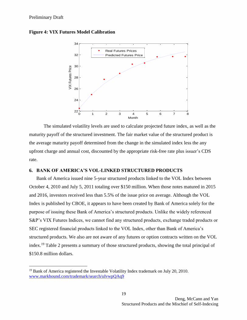
Figure 4 shows the model calibration using the VIX Futures data on September 22, 2010.

With all the parameters calibrated to the market, we simulate the daily instantaneous variances

for the next several years to cover the term of the investment. The four computed spot volatility

indexes are a function of daily instantaneous variances 𝑉𝑡 and the long term variance mean θt

viewed on the same day.18

18 The expected functional form for spot volatilities or forward volatilities futures are given in (Zhang, et

al., 2010). The expected value of spot variance (spot volatility squared) is essentially regarded as a

weighted average of current instantaneous variance and long term variance mean. The same functional

form is used in calibrating market VIX futures.

Preliminary Draft

19

Deng, McCann and Yan

Structured Products and the Mischief of Self-Indexing

Figure 4: VIX Futures Model Calibration

The simulated volatility levels are used to calculate projected future index, as well as the

maturity payoff of the structured investment. The fair market value of the structured product is

the average maturity payoff determined from the change in the simulated index less the any

upfront charge and annual cost, discounted by the appropriate risk-free rate plus issuer’s CDS

rate.

6. BANK OF AMERICA’S VOL-LINKED STRUCTURED PRODUCTS

Bank of America issued nine 5-year structured products linked to the VOL Index between

October 4, 2010 and July 5, 2011 totaling over $150 million. When those notes matured in 2015

and 2016, investors received less than 5.5% of the issue price on average. Although the VOL

Index is published by CBOE, it appears to have been created by Bank of America solely for the

purpose of issuing these Bank of America’s structured products. Unlike the widely referenced

S&P’s VIX Futures Indices, we cannot find any structured products, exchange traded products or

SEC registered financial products linked to the VOL Index, other than Bank of America’s

structured products. We also are not aware of any futures or option contracts written on the VOL

index.19 Table 2 presents a summary of those structured products, showing the total principal of

$150.8 million dollars.

19 Bank of America registered the Investable Volatility Index trademark on July 20, 2010.

www.markhound.com/trademark/search/uIvwpQAq9

0 1 2 3 4 5 6 7 822

24

26

28

30

32

34

Month

VIX

Fut

ures

Pric

e

Real Futures Prices

Predicted Futures Price

20

© Securities Litigation and Consulting Group, Inc.

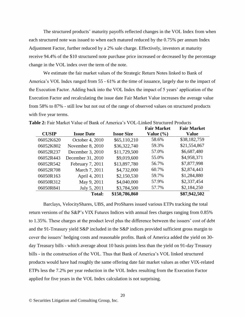
The structured products’ maturity payoffs reflected changes in the VOL Index from when

each structured note was issued to when each matured reduced by the 0.75% per annum Index

Adjustment Factor, further reduced by a 2% sale charge. Effectively, investors at maturity

receive 94.4% of the $10 structured note purchase price increased or decreased by the percentage

change in the VOL index over the term of the note.

We estimate the fair market values of the Strategic Return Notes linked to Bank of

America’s VOL Index ranged from 55 - 61% at the time of issuance, largely due to the impact of

the Execution Factor. Adding back into the VOL Index the impact of 5 years’ application of the

Execution Factor and recalculating the issue date Fair Market Value increases the average value

from 58% to 87% - still low but not out of the range of observed values on structured products

with five year terms.

Table 2: Fair Market Value of Bank of America’s VOL-Linked Structured Products

CUSIP Issue Date Issue Size

Fair Market

Value (%)

Fair Market

Value

06052K620 October 4, 2010 $65,110,210 58.6% $38,182,759

06052K802 November 8, 2010 $36,322,740 59.3% $21,554,867

06052R237 December 3, 2010 $11,729,500 57.0% $6,687,480

06052R443 December 31, 2010 $9,019,600 55.0% $4,958,371

06052R542 February 7, 2011 $13,897,780 56.7% $7,877,998

06052R708 March 7, 2011 $4,732,000 60.7% $2,874,443

06050R163 April 4, 2011 $2,150,530 59.7% $1,284,880

06050R312 May 9, 2011 $4,040,000 57.9% $2,337,454

06050R841 July 5, 2011 $3,784,500 57.7% $2,184,250

Total: $150,786,860 $87,942,502

Barclays, VelocityShares, UBS, and ProShares issued various ETPs tracking the total

return versions of the S&P’s VIX Futures Indices with annual fees charges ranging from 0.85%

to 1.35%. These charges at the product level plus the difference between the issuers’ cost of debt

and the 91-Treasury yield S&P included in the S&P indices provided sufficient gross margin to

cover the issuers’ hedging costs and reasonable profits. Bank of America added the yield on 30-

day Treasury bills - which average about 10 basis points less than the yield on 91-day Treasury

bills - in the construction of the VOL. Thus that Bank of America’s VOL linked structured

products would have had roughly the same offering date fair market values as other VIX-related

ETPs less the 7.2% per year reduction in the VOL Index resulting from the Execution Factor

applied for five years in the VOL Index calculation is not surprising.

Preliminary Draft

21

Deng, McCann and Yan

Structured Products and the Mischief of Self-Indexing

The Bank of America VOL-linked structured products were issued before the SEC began

requiring issue date fair value disclosures and so it was virtually impossible for investors to

know that Bank of America’s structured products were worth approximately 30% less than

alternatives from Barclays, VelocityShares, UBS, and ProShares.

7. JP MORGAN’S STRAT VOL-LINKED STRUCTURED PRODUCTS

JP Morgan first issued structured products linked to its proprietary Strat VOL Index and

Strategic Volatility Dynamic Index in July 2011, and continued to issue those structured products

in 2012, 2013, and 2014. JP Morgan issued at least 76 structured products that are linked to the

Strategic Volatility Index from 2011 to 2014. The total issue size of the structured products is

over $253 million.20 Table 3 lists the issue size and fair market value of the 10 largest JP Morgan

structured products linked to the Strat Vol and the remaining 66 issues size and fair market value

in the aggregate.

Table 3: Fair Market Value of JP Morgan’s Strat Vol-Linked Structured Products

CUSIP Issue Date Issue Size

JPM

Estimated

Value

Adjusted

Estimated

Value

Estimated

Value ($)

48125VQU7 3/13/2012 $23,642,000 N/A 84.92% $20,076,368

48126DZM4 3/4/2013 $14,159,000 N/A 85.44% $12,097,508

48125VEG1 11/30/2011 $13,473,000 N/A 83.98% $11,315,230

48125XE93 8/26/2011 $11,151,000 N/A 84.81% $9,456,770

48125VSH4 3/23/201221 $10,217,000 N/A 67.54% $6,900,816

48126NLV7 8/27/2013 $8,865,000 98.58% 85.53% $7,581,856

48125VWZ9 5/25/2012 $8,173,000 N/A 84.60% $6,914,587

48125VB58 6/26/2012 $7,387,000 N/A 84.69% $6,256,232

48125VPS3 3/27/2012 $7,174,000 N/A 85.11% $6,105,940

48125XYT7 7/26/2011 $6,503,000 N/A 85.39% $5,552,743

66 Smaller Notes $142,950,130 N/A 84.95% $121,438,487

Total: $253,694,130 84.23% $213,696,536

20 JP Morgan issued at least $32 million of structured notes linked to another Strategic Volatility Dynamic

Index from 2012 to 2013.

21 This is the only structured note issued with a term of 3-year, and the terms of the other notes are 2-year

or less.

22

© Securities Litigation and Consulting Group, Inc.

JP Morgan issued $109,550,130 of Strat Vol-linked structured products before the SEC’s

April 13, 2012 letter to issuers about, amongst other things, disclosure of issue date estimated

values. JP Morgan issued another $103,061,000 in Strat Vol linked structured products before it

started putting an issue date estimated value on the offering documents. Only $41 million of the

$254 million Strat Vol linked structured products were issued after JP Morgan started including

estimated issue date values.

JP Morgan’s estimated values have little relationship to the actual issue date values of the

Strat VOL-linked structured products because JP Morgan excluded the Rebalancing Adjustment

Amount from its valuations.

JPMS’s estimated value reflects the index fee that will accrue on a daily basis

over the term of the notes. The other adjustments to the level of the Index do not

impact JPMS’s estimated value.22

The only “other adjustments” to the level of the Index is the Rebalancing Adjustment

Amount. JP Morgan’s statement could be mis-interpreted to mean the other adjustments don’t

effect the value of the notes when what it actually means is literally that it doesn’t impact JP

Morgan’s estimate value because JP Morgan does not take into account the material, negative

impact of the Rebalancing Adjustment Amount on the Index and therefore on the future payoffs

and issue date estimated value of the notes. This is analogous to reporting an issue date estimated

value of a reverse convertible but not including the readily quantifiable value of the embedded

put option. Of course, that estimated value would be of a coupon note, not a reverse convertible.

As we demonstrated above, the Rebalancing Adjustment Amount reduces the Strat VOL

index and therefore the payoffs to JP Morgan’s structured products by at least 4.8% in every

possible state of the world and on average by 10.6% per year. Thus, JP Morgan overstates the

value of its Strat VOL-linked notes with a 15 month term by at least 6% with certainty when it

reports an estimated value of $987.64 per $1,000 and states. Accepting JP Morgan’s modeling of

the VIX term structure and other assumptions but simply incorporating the Rebalancing

Adjustment Amount, yields an 84.23% average issue date value. Most of the notes have 15

month terms. Taking into account the term of each note, the weighted average annual cost

embedded in the JP Morgan Strat Vol Notes was 12.1%. These are even higher than the average

annual costs in Bank of America’s VOL-linked notes.

22 See sp.jpmorgan.com/document/cusip/48126N3A3/doctype/Product_Termsheet/document.pdf.

Preliminary Draft

23

Deng, McCann and Yan

Structured Products and the Mischief of Self-Indexing

8. CONCLUSION

In structured products’ early days, issuers issued, underwriters underwrote and index

providers provided indexes. In the 1990s investment banks began issuing debt which looked a lot

like the convertible debt they had previously underwritten for operating companies. This allowed

for a proliferation of structured products but also created additional conflicts of interest as the

underwriter/issuer was not held to account for securities losses as operating companies who

issued convertible debt to investors were held to account for losses on the securities they issued.

The evolution of structured products continued with ever more complex structures tied to

stocks, indexes, commodities and baskets and then with proprietary indices including the two

VIX derived indices discussed herein. When brokerage firms include hypothetical trading costs

in their proprietary indices – costs that are absent from third-party indices – they make

comparison of disclosed costs at the structured product level uninformative. Even when issuers

are required to report issue date values, those values are uninformative if the issuer can value a

structured product based on an index that includes significant hypothetical costs but assume for

purposes of calculating an estimated value that the index was going to be calculated with no

trading costs thereby significantly inflating the value of the structured product. This mischief

would not be possible if issuers linked to indexes provided by third-party vendors who had no

interest in the payoffs from structured products linked to their indexes.

References:

Carr, Peter and Liuren Wu, “A Tale of Two Indices” Journal of Derivatives, 2006, 13(3), 13-29.

Deng, Geng, Craig McCann and Olivia Wang, “Are VIX Futures ETPs Effective Hedges?” with,

2012, Journal of Index Investing, 3(3):35-48, Winter 2012.

Lin, Yueh-Neng. “Pricing VIX futures: Evidence from integrated physical and risk-neutral

probability measures”, Journal of Futures Markets, 27(12):1175-1271, 2007.

Lin, Yueh-Neng and Chien-Hung Chang, “VIX Option Pricing” Journal of Futures Markets

29(6): 523-543, 2009.

Lin, Yueh-Neng and Chien-Hung Chang, “Consistent Modeling of S&P 500 and VIX

Derivatives” Journal of Economic Dynamics and Control 34(11):2302-2319, 2010.

Zhu, Song-Ping and Guanghua Lian, “Pricing Vix Options with Stochastic Volatility and

Random Jumps” Rivista di Matematica per le Scienze Economiche e Sociali 36(1), 2012.

Zhang, Jin E., Jinghong Shu, and Menachem Brenner, “The New Market For Volatility Trading",

The Journal of Futures Markets, Vol. 30, No. 9, 809-833 (2010).