student sorting and bias in value added estimationjrothst/publications/rothstein...student sorting...
TRANSCRIPT
Student sorting and bias in value added estimation:
Selection on observables and unobservables
Jesse Rothstein*
Princeton University and NBER
January 11, 2009
Abstract
Non-random assignment of students to teachers can bias value added estimates of teachers’
causal effects. Rothstein (2008a, b) shows that typical value added models indicate large
counter-factual effects of 5th grade teachers on students’ 4th grade learning, indicating that
classroom assignments are far from random. This paper quantifies the resulting biases in
estimates of 5th grade teachers’ causal effects from several value added models, under varying
assumptions about the assignment process. If assignments are assumed to depend only on
observables, the most commonly used specifications are subject to important bias but other
feasible specifications are nearly free of bias. I also consider the case where assignments depend
on unobserved variables. I use the across-classroom variance of observables to calibrate several
models of the sorting process. Results indicate that even the best feasible value added models
may be substantially biased, with the magnitude of the bias depending on the amount of
information available for use in classroom assignments.
* Industrial Relations Section, Firestone Library, Princeton NJ 08544. [email protected]. I thank Nathan Wozny and Enkeleda Gjeci for research assistance. I am grateful to the North Carolina Education Data Research Center and the North Carolina Department of Public Instruction for assembling and making available the data used in this study. This work has benefited from helpful conversations with Jane Cooley, Gordon Dahl, Ed Glaeser, Brian Jacob, David Lee, and Diane Schanzenbach, and from comments from an anonymous referee. Financial support was generously provided by the Industrial Relations Section and the Center for Economic Policy Studies at Princeton and by the U.S. Department of Education (#R305A080560).
1
1. Introduction
Proposals to consider teacher quality in hiring, compensation, and retention require
adequate measures of quality. This is increasingly defined in terms of educational outputs, as
reflected in student performance, rather than by teacher inputs like graduate degrees and
experience. In order for output-based quality measures to be of use, they must reflect teachers’
causal effects on the student outcomes of interest, not pre-existing differences among students
for which the teacher cannot be given credit or blame.
If students were known to be randomly assigned to teachers, there would be no
systematic differences in students’ potential outcomes across teachers, so straightforward
comparisons of mean end-of-year achievement would provide unbiased estimates of teachers’
effects.1 But there are many reasons for teachers not to be randomly assigned. Principals may
attempt to group students of similar ability together, so as to permit more focused teaching to
students’ skill levels, or they may try to spread high- and low-ability students across classrooms.
Teachers who are thought to be particularly skilled at teaching, e.g., reading skills may be
assigned students who are in need of extra reading help. Students who are known to create
trouble together may be intentionally assigned to different classrooms. Teachers who the
principal would like to reward may be given the easiest-to-teach students, with troublemakers
assigned to disfavored teachers in an effort to drive them away.2 Finally, parents, perceiving
teacher assignments as important determinants of their children’s success, may intervene to
ensure that their students are given a favored teacher or kept away from a disfavored one.
Given non-random assignments, the evaluation challenge in teacher effect modeling is to
distinguish teachers’ causal effects from the effects of pre-existing differences between the
students in their classrooms. If the determinants of classroom assignments are not adequately
controlled, teacher effect estimates will be biased. This bias is not averaged away even in large
1 There would still be the problem of accounting for sampling variation in the estimates: Because each teacher is in contact with only a few dozen students per year, annual estimates of teacher effects are quite noisy, and compensation schemes based on these estimates would have to be robust to the misidentification of teacher quality that results from this noise. But existing strategies – e.g., the Empirical Bayes approach used by Kane and Staiger (2008) or the similar Best Linear Unbiased Predictor used by the Tennessee Value Added Assessment System (Sanders and Horn, 1994) – suggest methods for doing this. 2 This aspect of assignments is likely to depend on the accountability metric in place: If teachers are rewarded for their value added and if value added estimates can be biased by systematic student assignment, the pattern of assignments is likely to change so that favored teachers benefit from this bias and disfavored ones are penalized.
2
samples, and existing methods for adjusting estimates for sampling error will not in general
remove its effects from teacher rankings.
The premise of “value added” models is that differences in the difficulty of the task faced
can be controlled by holding teachers responsible for students’ gains over the course of the year
rather than for their absolute end-of- year achievement levels. Rothstein (2008a, b) shows that
this is false. Students are sorted across classrooms in ways that correlated with both their score
levels and their gains. Specifically, 4th grade gains are highly non-randomly sorted across 5th
grade classrooms, with nearly as much across-class variation as in 5th grade gains. Because
annual achievement tends to revert quickly toward a student-specific mean, a student with a 4th
grade gain that exceeds the average by one standard deviation (SD) can be expected to fall short
of the average in 5th grade by about 0.4 SDs. Existing value added models attribute this shortfall
to the 5th grade teacher. A teacher assigned students with high 4th grade gains in the previous
year will look like a bad teacher through no fault of her own, while a teacher whose students
posted poor gains in the previous year will be credited for their predictable reversion to trend.
Although Rothstein (2008a, b) documents substantial non-randomness in teacher
assignments that violates the restriction of common value added models (hereafter, VAMs), he
does not directly estimate the magnitude of the resulting biases, and he provides little evidence
about the prospects for correcting them via more sophisticated controls for students’ past
achievement trends.3
This paper attempts to quantify the bias created by non-random assignment in several
value added specifications. Three conditions govern the bias. It depends first on the amount of
information available for use in the classroom assignment process about students’ potential end-
of-year achievement or annual gain, second on the importance attached to this information in
assignments, and third on the degree to which the control variables included in the value added
specification can absorb the information used in assignments.
Value added studies frequently distinguish between the effect of having a particular
teacher and the effect of being in a particular classroom, with the former included in the latter. I
take the classroom effect – the causal effect of being in one classroom as opposed to another in
3 Rothstein (2008a, b) does demonstrate that unbiased estimation requires controls for dynamic student achievement: Teacher assignments are not governed solely by permanent student characteristics, but respond dynamically to each year’s test scores. This rules out fixed effects solutions like those used by Harris and Sass (2006); Koedel and Betts (2007); Jacob and Lefgren (2008); Rivkin et al. (2005); and Boyd et al. (2008).
3
the same school – as the parameter of interest.4 This avoids the problem of distinguishing
different components of the classroom effect, the most obvious being the effects of teacher
quality and of peers. This problem is complex even when classroom assignments are random and
is much more so with non-random assignments. But the identification of classroom effects is a
necessary precondition for the larger problem of isolating teachers’ causal effects, and by
focusing on this smaller, first problem I can place a lower bound on the bias in estimates of
teachers’ effects that is produced by the assignment process.
I distinguish between two forms of non-random assignments: Those that depend only on
variables which are observed by the analyst, with random assignment conditional on those, and
those that depend as well on information known to participants in the assignment process but not
observed by the researcher. In the former case, “selection on observables,” bias in classroom
effect estimates can be measured directly. In the latter, the magnitude of the bias can be
quantified only with assumptions about the amount and nature of information that is used in
classroom assignments. I take an approach that is in the spirit of Altonji, Elder, and Taber’s
(2005; hereafter AET) assumption that sorting on unobserved variables resembles sorting on
observables, though the specific assumptions differ: Where AET assume that sorting is incidental
and is equally correlated with observed and unobserved determinants of the outcome variable of
interest, I assume that the sorting is intentional and that it depends on a limited set of predictors
that are observed by the school principal,5 a subset of which are observed by the researcher as
well. AET’s assumption represents a limiting case for my analysis, in which the principal can
perfectly predict students’ end-of-year achievement and gains before making teacher
assignments. I also consider several more plausible scenarios for the principal’s role in
assignments.
Section 2 describes the data. In Section 3, I demonstrate that past test scores and
behavioral variables are strongly predictive of future achievement and achievement gains.
Section 4 summarizes the evidence from Rothstein (2008a, b) that teacher assignments are
4 If a teacher’s assignments are uncorrelated across cohorts – that is, if a teacher who gets high-potential-gain students this year is no more or less likely than any other teacher to get high-potential-gain students next year – then studies that examine several cohorts of students for the same teacher can convert bias in the classroom effect into mere sampling error in the teacher’s effect. But this uncorrelated assignments assumption is a strong one, and it does not appear to hold – even approximately – in the North Carolina data used here. 5 For simplicity, I discuss class assignments as the outcome of principals’ decisions. This is not meant to restrict the principal to be the only determinant of these assignments; the principal’s decision might reflect input from parents, teachers, and the student itself.
4
importantly correlated with past scores. In Section 5, I examine the bias that arises in several
common value added models if classroom assignments are random conditional on the observed
variables. Section 6 describes the methodology for assessing the bias that arises if parents and
principals have more information about students’ potential learning growth than is available in
research data sets. Section 7 presents the results of the analysis of selection on unobservables.
Section 8 concludes.
2. Data
I work with longitudinal administrative data on students in public elementary schools in
North Carolina, assembled and distributed by the North Carolina Education Research Data
Center. North Carolina has been a leader in the development of linked longitudinal data on
student achievement, and the North Carolina data have been used for several previous value
added analyses (Clotfelter, Ladd, and Vigdor 2006; Goldhaber 2007).6
I focus on the value added of 5th grade teachers in 2000-2001. I use annual end-of-year
tests that were given in grades 3-5, as well as “pre-tests” given at the beginning of grade 3. The
tests purport to use a “developmental” scale, and the score scale is intended to be meaningful
(i.e. scores are cardinal and not simply ordinal measures) both across grades and across the
distribution within grades.7 I standardize scores so that the population mean is zero and the
standard deviation one in 3rd grade; by using the same standardization in all grades I preserve
the comparability of scores across grades.
The North Carolina data do not identify students’ teachers directly, but they do identify
the person who administered the end-of-grade tests. In the elementary grades, this was usually
the regular teacher. I follow Clotfelter, Ladd, and Vigdor (2006) in using a linked personnel
database to identify test administrators with regular teaching assignments. I count a match as
valid if the test administrator taught a self-contained (all day, all subject) 5th grade class that was
not coded as Special Education or Honors and if at least half of the tests that she administered
6 North Carolina was one of the first two states approved by the U.S. Department of Education to use “growth-based” accountability models in place of the status-based metrics that are otherwise required under No Child Left Behind. 7 It is not clear that a scale with this property is even possible (Martineau, 2006), or even if it is how one would know whether a test’s scale has the property. Nevertheless, value added modeling as typically practiced is difficult to justify if scores are not interval scaled both across and within grades. See Ballou (2002) and Yen (1986). The analysis here is not sensitive to violations of this property, though if it does not hold the value added estimators considered (here, and elsewhere in the literature) are difficult to justify. See Rothstein (2008a).
5
were to 5th grade students. 73% of 5th grade tests were administered by teachers who are valid
by this definition.
My analysis focuses reading scores, though similar results obtain for math scores. My
sample consists of students who were in 5th grade in 2000-2001, who had a valid teacher
assignment in that year, and for whom I have complete test score data in grades 3-5. Table 1A
presents summary statistics and a correlation table for reading scores on the 3rd grade pretest and
on the end-of-grade tests in 3rd, 4th, and 5th grades, as well as for the 5th grade gain score
(defined as the difference between the 4th and 5th grade scores). Mean scores in my complete-
data sample are about 0.07 standard deviations higher than in the population in every grade.
Scores are correlated about 0.80 in adjacent grades (lower for the 3rd grade pre-test, which is
substantially shorter), with slightly reduced correlations across longer time spans. 5th grade gains
are weakly positively correlated (+0.07) with 5th grade score levels and strongly negatively
correlated (-0.52) with 4th grade scores. They are notably negatively correlated (-0.25) with 3rd
grade scores as well.
Observed scores are noisy measures of true achievement. The degree of measurement
error in test scores is usually measured by the “test-retest reliability,” the correlation between
students’ scores on alternative forms of the same test administered a short interval apart.8 A 1996
report estimates that the test-retest reliability of the North Carolina 7th grade reading test is 0.86
(Sanford 1996, p. 45). Unfortunately, test-retest studies have not been conducted for other
grades. Under the assumption that individual item reliability is constant across grades and that
item responses are independent, the 7th grade reliability can be extended to the shorter tests in
earlier grades.9 Doing so, I estimate that the grade-3 pre-test has reliability 0.72, the grade-3 end-
of-grade test has reliability 0.84, and the tests in grades 4 and 5 have reliability 0.86. I treat these
as known, without sampling error.10
8 Test makers often report alternative measures of reliability, e.g. internal consistency measures that are based on correlations between a student’s scores on different subsets of questions. The internal-consistency reliabilities for the tests in grades 3, 4, and 5, respectively, are 0.92, 0.94, and 0.93 (Sanford, 1996, p. 45). The corresponding statistic for the grade-3 pre-test used for the cohort under consideration is not reported, but a more recent form of the test has reliability 0.82 (as compared with 0.92 in on the corresponding tests in grades 3-5; see Bazemore, 2004, p. 63). These statistics are computed under the assumption that responses are independent across questions; common shocks (e.g. a cold on test day) would lead these methods to overstate the test’s reliability. 9 If item responses are not independent, reliability will be less sensitive to test length, and I will most likely understate the reliability of the (relatively short) 3rd grade pretest. 10 The sample for the test-retest study was only 70 students, in 3 classrooms. If the 70 observations are independent, an approximate confidence interval for the grade-7 test reliability is (0.78, 0.91), though within-classroom
6
A known reliability allows me to compute summary statistics for true achievement, net of
measurement error, assuming that errors are independent across grades. These are reported in
Table 1B. The correlation between a student’s true achievement in adjacent grades is
approximately 0.96. The 5th grade gain is strongly negatively correlated with achievement levels
in all grades.
One can examine across-grade correlations in gain scores as well as in score levels. The
correlation between observed grade-4 and grade-5 gains is -0.42. Measurement error in the
annual test scores biases this downward, but even when corrected the correlation remains
negative. Thus, students with above-average gains in grade 4 will, on average, have below-
average gains the following year. To the extent that such students are systematically assigned to
particular teachers, value added models that fail to account for this mean reversion will be biased
against those teachers.
3. Predictions of grade 5 achievement and gains
The relevance of classroom assignments for value added estimation depends crucially on
the degree to which students’ gains are predictable based on prior information. If 4th grade
characteristics are entirely unpredictive of 5th grade gains, then even assignment on the basis of
those characteristics will not create bias in 5th grade value added models. Table 2 presents
several specifications for students’ reading scores at the end of grade 5, using prior scores and
other predetermined variables as explanatory variables. Because it is almost certainly more
difficult to control for the sorting of students across schools than within, and because I focus in
this paper in identifying differences in teachers’ effects within schools, I consider only
specifications for within-school variation in 5th grade scores. The first column shows that 87%
of the variance in 5th grade scores is within schools. Column 2 adds the 4th grade reading score.
This has a coefficient of 0.680; neither zero nor one is within the confidence interval. The
inclusion of the 4th grade score increases the model’s R2 by 0.55; 4th grade scores explain 63.5%
of the within-school variation in 5th grade scores.
Column 3 adds to the specification reading scores from the beginning and end of grade 3.
Both are significant predictors of 5th grade scores. Their inclusion lowers the 4th grade score
dependence would imply a wider interval. Note also that a given test will have higher reliability in a heterogeneous population than in a homogeneous one. The likely homogeneity of the test-retest sample suggests that the reliability in the population of North Carolina students is probably higher than was indicated.
7
coefficient by about one third, and raises the within-school R2 by 0.045. Column 4 adds three
lagged scores on the math exam. Again, all are significant. The within-school R2 is 0.058 higher
than in the specification with just a single lagged reading score. Column 5 adds 28 additional
covariates, measured in grade 4, that might help to predict students’ grade-5 achievement. These
include race, gender, and free lunch status indicators; measures of parental education; various
categories of “exceptionality” and learning disabilities; and measures of the time spent on
homework and watching TV. These are jointly highly significant, though their inclusion raises
the explained share of variance by only 0.003.
The available variables –nearly all of which were readily observable when students were
assigned to 5th grade classrooms – explain nearly 70% of the within-school variation in students’
grade-5 test scores. Moreover, this substantially understates the predictability of student
achievement. Recall from Section 2 that 14% of the variance in observed 5th grade scores is
noise that would not even persist into a second administration of the test a week later. This noise
is irrelevant to the predictability of achievement, and is uncorrelated with all predictor variables.
Table 2 also shows estimates of the explained share of the within-school variance of true
achievement, net of this transitory noise. These range from 0.764 with just the 4th grade score to
0.837 with the full set of controls.
Of course, predictions of end-of-year scores are easy: It should not be surprising that
students who score highly in 4th grade tend to continue to earn high scores in 5th grade, and all
value added models control for this variation in one way or another. A harder task is to predict
5th grade gains. So long as the 4th grade score is included as a covariate, the coefficients in a
prediction equation for gains are identical to those for levels, save that the 4th grade score
coefficient is reduced by 1. But the explained share of variance is much lower. The bottom rows
of the Table show the R2 statistics for specifications that take grade-5 gains as the dependent
variable. These range from 0.279 to 0.398 within schools. The first-difference transformation
does not eliminate predictability; the principal clearly has substantial information at his disposal
for the prediction of student gain scores.11
11 Neither coefficients nor fit statistics can be directly converted to those that would be seen for the true gain score, net of measurement error, because measurement error in the 4th grade score appears on both sides of the equation for 5th grade gains. I discuss in Section 6 how the coefficients of specifications for true gains can be recovered from the estimates in Table 2. True gains are quite predictable as well.
8
Also relevant to the analysis below is the value of past gains for predicting future scores
and gains. Table 3 presents specifications using grade-4 gains as explanatory variables. These
explain only 0.2% of the within-school variance in 5th grade achievement but 18.2% of the
variance in 5th grade gains.
4. Evidence for non-random assignment
The simplest value added model estimates each teacher’s effect as the average gain score
of her students.12 In order to attribute this average gain to the teacher, it must be the case that the
information used to make teaching assignments is uninformative about students’ potential gains,
conditional on any control variables. As shown in Section 3, prior achievement and gains are
strongly predictive of future scores and gains, so correlations between teacher assignments and
past gains would violate the simple VAMs identifying assumption. Rothstein (2008a, b) tests for
“effects” of 5th grade teachers on 4th grade gains. Given the evidence in Table 3, effects of this
sort would indicate that expected 5th grade gains are not balanced across 5th grade classrooms,
and that the simple VAM will be biased.
Let Aig be the test score for student i at the end of grade g. The grade-g gain is defined as
∆Aig ≡ Aig − Ai,g−1. Let Sig be a vector of indicators for the school attended in grade g and let Tig
be a set of teacher indicators. The simple value added model is based on the regression of gains
on school and teacher indicators, with the teacher coefficients normalized to mean zero within
each school:
∆Aig = Sig αg + Tig βg + εig. (1)
In order for this regression to yield unbiased estimates, unobserved determinants of annual gains
must be uncorrelated with Tig. I evaluate this assumption by substituting in (1) the student’s gain
in some prior year h < g:
∆Aih = Sig αh + Tig βh + εih. (2)
The causal effect of the grade-g teacher on the gain in grade h is necessarily zero. A nonzero
coefficient βh can therefore arise only if the error in grade h, εih, is correlated with the grade-g
teacher assignment; that is, if teacher assignments in grade g depend on past outcomes. As we
12 This is not a widely used model. However, it is quite similar to the implicit model of the most widely used VAM, the Tennessee Value Added Assessment System (TVAAS; see Sanders et al., 1997). This is specified as a mixed model for level scores that depend on the full history of classroom assignments, but its identifying assumption is essentially that the simple model that I consider here is an unbiased estimator of teachers’ causal effects.
9
have seen, εih is correlated with εig, so any such correlation means the simple value added model
will yield a biased estimate of the effect of the grade-g teacher on the grade-g gain.13
Table 4 presents estimates of 5th grade teachers’ coefficients in models for gain scores in
grades 5, 4, and 3, using specifications (1) and (2). To permit comparisons across models, I use a
balanced panel of students who attended the same school for all three grades. These are similar
to those reported in Table 3 of Rothstein (2008a), albeit estimated from a slightly different
sample.
We begin with the model for grade-5 gains. The 3,013 elements of the vector
(normalized to mean zero across all 5th grade teachers at the school) can be summarized by their
standard deviation. This, 0.152, is shown in Column 1.
β̂5
14 I also report an adjusted standard
deviation that subtracts from the across-teacher variance the contribution of sampling error to
this variance (Aaronson, Barrow, and Sander 2007; Rothstein 2008a). This adjusted standard
deviation, which estimates the variability of the true β coefficients net of sampling error, is
0.107: A teacher who is one standard deviation better than average has students who gain 1/10 of
a standard deviation (of achievement levels) relative to the average over the course of the year.
This resembles existing estimates (Aaronson, Barrow, and Sander 2007; Kane, Rockoff, and
Staiger 2008; Rivkin, Hanushek, and Kain 2005).
The remaining columns present counterfactual estimates that vary only the dependent
variable. Column 2 presents estimates for 4th grade gains. We know that there are no causal
effects of 5th grade teachers on 4th grade gains (i.e. that β4 = 0), so any non-zero coefficients in
this specification are indicative of student sorting. The hypothesis that β4 =0 is decisively
rejected, and indeed there is nearly as much variation in the elements of ~β4 as in those of : The
sampling-adjusted standard deviation of 5th grade teachers’ normalized “effects” on 4th grade
gains is 0.080, nearly as large as that for 5th grade gains. Column 3 presents an analogous model
where the dependent variable is the 3rd grade gain, the difference between the student’s score on
β̂5
13 Rothstein (2008b) formalizes the test and discusses its interpretation in greater detail than is possible here. Note that the grade-h teacher is a potential omitted variable in (2), and a correlation between Tig and Tih could yield a non-zero βh even if grade-g classroom assignments do not depend on εih. Rothstein (2008b) shows that the inclusion of controls for Tih has essentially no effect on the results. 14Across-teacher means and standard deviations are weighted by the number of students taught, and degrees of freedom are adjusted for the normalization of . Further details of the methods are available in Rothstein (2008a). β5
10
the end-of-grade reading test and the beginning-of-the year pretest. We see even larger apparent
effects of 5th grade teachers here.
The lower portion of Table 4 presents correlations between the estimates of the
coefficient vectors β5, β4, and β3, first unadjusted for sampling error and then adjusted. Adjacent
coefficients are highly negatively correlated, both before and after the adjustment for sampling
error, but there is nearly no correlation between β5 and β3.
Two of these correlations are of particular interest here. First, corr (β5, β4) = −0.35. This
indicates that 5th grade teachers who appear (by the simple model 1) to have high value added
tend to be those whose students experienced below-average gains in grade 4. As noted earlier,
gains are negatively autocorrelated at the student level; at least a portion of the variation in
estimated 5th grade value added apparently reflects predictable consequences of non-random
student assignments.
The second interesting correlation is that between β4 and β3, -0.36. One hypothesis that
could explain the presence of counterfactual “effects” of 5th grade teachers on earlier grades’
gains is that students differ systematically in their rate of gain, and that classroom assignments
depend in part on that rate. Rothstein (2008a) refers to this explanation as “static tracking”–the
determinants of classroom assignments are constant across grades, and conditional on these
determinants the test score in grade g does not affect the teacher assignment in g+1. In the
presence of static tracking, the bias in teacher effects coming from non-random assignment can
be absorbed by pooling data on a student’s gains across several grades and including student
fixed effects in the specification. This sort of specification is used by Harris and Sass (2006);
Koedel and Betts (2007); Jacob and Lefgren (2008); Rivkin, Hanushek, and Kain (2005); and
Boyd et al. (2008), among others.
As Rothstein (2008a) notes, static tracking implies that in simple specifications like those
in Table 4 the coefficients for the grade-g teacher on gains in grades h and k (h, k < g) should be
identical, up to sampling error. In other words, corr (β4, β3) = 1.15 This restriction does not even
approximately hold in the data. Classroom assignments are evidently not made on the basis of
permanent student characteristics, but respond dynamically to annual student performance. This
implies that student fixed effects specifications provide inconsistent estimates of teachers’ causal
15 Again, this conclusion is supportable only if the correlation between β4 and β3 is negative in specifications that include controls for 4th and 3rd grade teachers, where those in Table 2 do not. The correlation is nearly identical when these controls are included.
11
effects. The only way to control for non-random classroom assignments while permitting
consistent estimation of teachers’ effects is to measure the determinants of assignments directly.
Many value added specifications (e.g., Gordon, Kane, and Staiger 2006; Kane, Rockoff,
and Staiger 2008; Aaronson, Barrow, and Sander 2007; Jacob and Lefgren 2008) control for the
baseline score, in effect modeling the end-of-year score as a function of the beginning-of-year
score and the teacher assignment. These specifications are robust to dynamic teacher
assignments of a very restricted form: Unless teacher assignments are random conditional on the
baseline score, estimates will still be biased. The estimates in Tables 2 and 3 indicate that there is
a great deal of information available to principals about students’ potential gains above and
beyond that provided by the lagged score; there is no reason to expect that the use of this
information in forming classroom assignments can be absorbed with simple controls. I show
below that the once-lagged-score specification is rejected by the data.
5. Selection on observables
Strategies for isolating causal effects in the presence of non-random assignment of
treatment (in this case, of classroom assignments) depend importantly on whether the
determinants of treatment are observed or unobserved. Accordingly, I treat the two cases
separately. I defer discussion of the selection-on-unobservables case to Section 6. In this Section,
I assume that selection is solely on observables: 5th grade teacher assignments are random
conditional on the available variables measured in 4th grade. Under this assumption, bias can be
avoided by controlling for the full set of observables in the value added model. Models that use
less complete controls may be biased if the included variables are unable to absorb all of the non-
randomness of teacher assignments. Note that no harm is done by controlling for variables that
are not used in teacher assignments. Accordingly, I allow teacher assignments to depend on any
or all of the variables included in Column 5 of Table 2 – the history of math and reading test
scores plus a set of demographic and behavioral variables as measured in grade 4. I label these
variables Xi4. If 5th grade classroom assignments are in fact random conditional on Xi4, then the
effects of 5th grade teachers can be estimated via a simple regression of 5th grade gains on 5th
grade school and teacher indicators with controls for the Xi4 variables:
∆Ai5 = S i5 α + T i5 β + X i4 γ + εijs5. (3)
12
Note that 4th grade reading and math scores are included in Xi4. Thus, (3) is identical to a
regression that uses the 5th grade score (rather than the gain) as the dependent variable, as this
simply adds Ai4 to both sides.
Value added models (hereafter, VAMs) rarely have access to the full set of control
variables included in Xi4. Omission of any variable that influences classroom assignments may
produce bias in the estimated teacher effects. To evaluate the importance of this – under the
maintained assumption of selection-on-observables – I compare estimates from (3) with those
obtained from three VAMs with less complete controls:
VAM1: Ai5 = S i5 a + T i5 b + e i5
VAM2: ∆Ai5 = S i5 a + T i5 b + e i5
VAM3: ∆Ai5 = S i5 a + T i5 b + A i4 c + e i5
VAM4: ∆Ai5 = S i5 a + T i5 b + A i4 c4 + A i3 c3 + A i2 c2 + e i5
VAM1 credits each teacher with the average achievement of students in her class (less the
school-and-grade-level average). I include this “levels” specification, which few would advocate,
solely as the basis for comparison to more reasonable models. VAM2 effectively controls for
students’ 4th grade scores, constraining their coefficients to one. Teachers are credited with
students’ average gain scores (again relative to the school-grade average). This is the basic
specification used in most value added policy and above in Section 4. VAM3 controls for
students’ 4th grade achievement and estimates the coefficient on the lagged score rather than
constraining it to one. In this model, teachers are credited with their students’ performance
relative to other students in the same school and grade with the same beginning-of-year scores.
Finally, VAM4 controls not just for last year’s score but for the two prior scores as well. (The 3rd
grade pre-test is denoted Ai2 here.) This sort of specification is not widely used. It could in
principle be used in some value added implementations, though unavoidable data limitations
would prevent its widespread adoption. Most importantly, this VAM is not available for the
assessment of teachers in the first three grades in which students are tested.
For each model, I compute the standard deviation across teachers of b and of the bias
relative to the coefficient vector from the richer specification (3), b – β. A useful summary
statistic is the variance of the bias relative to that of teachers’ “true” effects (as indicated by (3)),
V(b − β) ⁄ V(β). I also compute the correlation between the bias and the true effect, corr (b − β,
β): It is helpful to know whether good teachers (at least as indicated by the baseline model (3))
13
are helped or hurt by the assignment process. A strong positive correlation between true effects
and the bias would imply that teacher rankings are not much affected by sorting bias, while a
negative correlation would indicate that biases from non-random assignments mask differences
in true teacher quality.
Table 5 presents the results. Each statistic is computed first from the estimated
coefficients (in the first panel), then adjusted for the influence of sampling error (second panel).
The baseline specification indicates that the standard deviation of teachers’ effects is 0.096, or
0.124 before the adjustment for sampling error. VAM1 indicates much more variability of
teacher effects, though this is primarily bias–the bias in this specification is more than three
times as large (in variance terms) as the true variability that we are attempting to measure. The
specification for gain scores, VAM2, eliminates much of the bias, but its variance is still half that
of the true effects. VAM3, controlling for the 4th grade score, cuts the standard deviation of the
bias in half; here, the variance of the bias is 13% of that of the quality signal. This is small in
comparison with the previous models, but still substantial enough to represent a problem for
policy. In each case, biases are only weakly correlated with true coefficients.
VAM4 eliminates nearly all of the bias relative to the richer selection-on-observables
specification. This is unsurprising: Recall that Table 2 indicated that the control variables
included in (3) but excluded from VAM4 added only 0.3%to the explained share of variance of
5th grade achievement and 0.6% to the explained share of variance of 5th grade gains. Thus, my
assumption that specification (3) permits unbiased estimation of teachers’ causal effects implies
that omitted variables bias in VAM4 is negligible. To understand the true potential for bias in
this specification, we will need to consider the impact of selection on information that is
unobserved in my sample but is available for use in forming classroom assignments. I develop
methods for assessing this in the next Section.
6. A model of tracking on unobservables
There is no good reason to think that classroom assignments depend only on the variables
available in my data. Indeed, the presence of noise in the observed test score history strongly
suggests otherwise. A principal or parent would almost certainly be able to form a less noisy
measure of students’ achievement each year by combining test scores with other measures (e.g.
grades) that I do not observe. In this Section I develop a framework in which classroom
14
assignments depend on the observed variables and on unobserved variables that have known
correlations with the observables. This permits computation of the variance across teachers of the
bias in feasible estimates of β, though not the bias in any individual teacher’s estimated effect.
In the selection-on-observables analysis in Section 5, I allowed for the possibility that
classroom assignments depended on only a subset of the observed variables. The cost of
allowing for selection on unobservables is that we must rule that possibility out: I require here
that the set of variables that influence classroom assignments be known precisely. I assume that
assignments depend on an index formed by averaging a set of pre-specified variables with
weights that best predict student outcomes. Assignments are assumed to be uncorrelated with
later outcomes conditional on this index.
I assume that the researcher is able to observe some but not all of the variables from
which the prediction index is formed. When all of the predictor variables are observed, the setup
collapses to the selection-on-observables model discussed in Section 5. When only a subset is
observed, the distribution of the observed variables across classrooms can be used to identify the
importance of predicted outcomes, relative to the residual, in forming classroom assignments.
I develop the model in several parts. I begin by describing the assumed assignment
process, then discuss the implications of these assignments for VAM estimation, and finally
describe how the North Carolina data can be used to calibrate the model and to estimate the
degree of bias in feasible VAMs that is implied by the assumed assignment process. The model
is presented in terms of a principal who uses the information available to her to make classroom
assignments. This is shorthand. Classroom assignments may depend on negotiation between
principals, teachers, students, and parents, each of whom may observe different aspects of the
student. The “principal” in my model is a black box that takes all of the information available to
the various agents and outputs a classroom assignment.
6.1. Classroom assignments
I assume that the principal observes three classes of characteristics for each student: Z,
characteristics that are useful predictors of student outcomes and that are observed as well by the
data analyst; W, predictor variables that are not observed by the analyst; and η, determinants of
classroom assignments that are not predictive of the academic outcomes analyzed in value added
models. Let Y represent the outcome. Y might measure true gains or observed gains; we will see
below that this has important consequences for the analysis.
15
We can distinguish between the teacher’s true causal effect, Tβ, and the other
components of the outcome, ω = Y − Tβ. The challenge in value added modeling is that the
classroom assignment T may depend on ω, or at least on that part of ω that is known to the
principal. Let I ≡ E[ω | Z, W] be the principal’s prediction of ω, and let ε = ω − I. We can
measure the amount of information available to the principal by V(I)/V(ω) = σI2 ⁄(σI
2 +σε2).
I assume that classroom assignments depend on Z and W only through the index I. This is
central to my strategy, as it enables me to recover the amount of sorting on the unobserved
variables W by measuring the degree of sorting on the observed variables Z. Assignments may
depend in part on the non-predictive variables, η, however. It is convenient to normalize η to be a
single variable that is orthogonal to all other variables (i.e. to Z, W, and ε) and is scaled so that
assignments depend on the simple sum λ ≡ I + η. Because η is never observed by the analyst, this
carries no loss of generality. I also impose the more restrictive assumption that {I, η, ε} are
jointly normally distributed.
Students are sorted perfectly on λ into classes.16 That is, all of the students assigned to a
particular teacher have the same λ value. The importance of predicted outcomes in assignments
is controlled by ση2: If the principal assigns students to classrooms solely on the basis of
predicted outcomes, ση2 = 0 and λ ≡ I. Perfect random assignment represents the opposite
limiting case, ση2 = ∞ and λ ≈ η. The across-classroom variance of I is the difference between the
total variance and the within-classroom variance, V(I) −V(I | λ) = corr2(I, λ)V (I) = σI 4⁄(σI
2 +
ση2). This is large if predicted outcomes are the primary determinants of assignments and small if
they are relatively unimportant.
6.2. The principal’s prediction
In order to make further progress, we need to specify the information available to the
principal for use in predicting outcomes (i.e. the variables Z and W). I consider several scenarios
in the empirical analysis below. Intermediate cases between selection-on-observables and perfect
predictability of future outcomes are the most realistic and I focus on these, though I also include
16 This is at best an approximation. A typical school has three to five classes per grade; even if these classes are perfectly stratified, λ will have considerable heterogeneity within classes. With less than perfect sorting, my methods will understate the importance of I (relative to η) in classroom assignments and therefore will understate the bias in value added models due to these assignments. The basic approach could be extended to stratification on λ across a finite number of classes (so that one class has students with λ ∈ (−∞, c1), another has λ ∈ (c1, c2), etc.), at the cost of considerable additional complexity.
16
the limiting cases for comparison. I begin with base cases in which selection is on observables,
as in Section 5:
A. The principal has no information about future achievement gains beyond that
contained in the 4th grade test score (Z = {A4}; W = {ø}).
B. The principal observes the test score history, but has no additional information about
achievement gains (Z = {A2, A3, A4}; W = {ø}).
Note that scenarios A & B are falsified by the evidence in Table 2: Since the principal can
observe all of the 4th grade variables that are available in my data, the fact that these variables are
useful in predicting gains indicates that the principal has more information about potential gains
than just the score history. Nevertheless, these scenarios provide useful baselines.
A second set of scenarios allows the principal to be better able to disentangle the signal
and noise components of the test score history than can the econometrician. The principal knows
students and has access to course grades and other indicators of student achievement with which
to do this. A useful parameterization is to assume that the principal has access to k additional test
score histories, each subject to its own error but with errors independent across tests. That is, if
the true achievement history through 4th grade is A* = (A1*, . . . , A4
*), we assume that the value
added analyst observes only the measured achievement history A = A* + u. The principal
observes this as well, but also sees additional series {q1, q2, . . . , qk}. Each measures true
achievement with independent error: qj = A* + vj, E[v'j vj] = E[u'u], and E[v'j vh] = E[v'j u] = 0.
The q series can be thought of as representing grades, student evaluations, or classroom
observations that are available to the principal but not reported in typical data sets.
C. The principal observes the test score history that is available to the analysis, and also
observes k additional noisy achievement series (Z = {A}; W = {q1, . . . , qk}).
In the limit as k → ∞, this scenario converges to:
D. The principal observes both the test score history and the true achievement history (Z
= {A}; W = {A*}).
Note that the history of observed scores is not redundant in scenario D: When Y is the observed
gain, the lagged observed score is informative about the measurement error component in ω (i.e.
about ∆Ag− ∆Ag*= ug− ug−1).
Even scenarios C and D are quite restrictive. As we will see, the true achievement history
explains only a third of the within-school variance of true achievement gains, and it is plausible
17
that the principal, who knows something of the child’s family situation and emotional and
cognitive development patterns, has information about the remaining portion.
E. The principal observes the test score history, the true achievement history, and an
additional orthogonal signal of ω (Z = {A}; W = {A*, G}).
Results here will depend on the quantity of information that this additional signal is assumed to
contain. Let the principal’s prediction regression be
E[ω | A, A*, G] = Aφ + A*χ + Gψ.
Then we can index the information in G by f = V(Gψ)/V(A*χ). The limiting case (as f →
V(ω | A*)/V(A*χ)17) is:
F. The principal can predict the outcome perfectly (Z = {A}; W = {ω}).
Note that this does not imply that students are perfectly sorted across classrooms on the basis of
their potential outcomes. Recall that the principal is assumed to combine her prediction with an
orthogonal term η and sort only on that combination. A principal who could perfectly predict
outcomes might still assign poorly-sorted classes if she thought ability-mixing was desirable or if
her goal of tracking students by ability was balanced against other objectives. Either would
correspond to a large ση2.
Even so, F is not a plausible scenario for the problem at hand, as it is not realistic to
suppose that principals can perfectly predict how well students will do over the course of a year.
I include it because it illustrates the connection between the methods used here and those used by
AET. Where in the earlier scenarios the principal observed all of the variables available to the
analyst plus a subset of the remaining component of students’ gains, here the principal observes
both components equally. As a result, both are equally sorted across classrooms. This
corresponds to AET’s assumption that selection on unobservables is identical to selection on
observables.18
The six scenarios are summarized in Table 6.
6.3. Bias in under-controlled value added models
17 When Y is the true gain and teachers have no true effects, this corresponds to f → (1− R2)/R2, where R2 is the explained share of variance from a regression of ∆A* onto A*. As I discuss below, R2 is about 0.34. Thus, this limit is just below 2. 18 Altonji et al. also consider intermediate cases, where the correlation between the unobserved determinants of selection and outcomes lies between zero (no selection) and the value corresponding to scenario F. The above framework can be seen as providing a basis for the choice of this correlation.
18
We can write outcomes as the sum of teacher effects, the principal’s prediction I, and the
portion of outcomes that the principal was unable to predict:
Y = a + Tβ + I + ε. (4)
Because I is a determinant of classroom assignments, it is correlated with T. That is, there are
differences across classrooms in student outcomes that do not reflect teacher quality.
Unbiased estimation of β requires controlling for I in a value added model specified as
(4).19 Unfortunately, (4) is not a feasible value added model. In most of the scenarios described
above, the analyst observes only a subset of the variables used to construct I. The inability to
control fully for I produces bias in the resulting estimates.
It is easiest to characterize the bias in VAM2, which does not include any controls. I is an
omitted variable here, and any across-classroom component of it represents bias in . The
variance of this bias is equal to the across-classroom variance of I, σI 4⁄ (σI
2 + ση2).
β
In a richer VAM that includes control variables Z, these variables may absorb some of the
bias. Write the regression of I onto T and Z as I = Tκ + Zπ + ν.20 We can rewrite (4) as
Y = a + T (β + κ) + Zπ + (ν + e). (5)
By construction, the terms in the final parentheses are uncorrelated with both T and Z, so do not
create bias in the coefficients. But notice that the T coefficient here combines the causal effect β
with an additional bias term, κ. This reflects the fact that the principal is able to predict the
outcome better than can the analyst and that he uses his superior prediction in forming classroom
assignments. The structure developed above makes it possible to derive the magnitude of the bias
(i.e., V(Tκ)). Intuitively, sorting of students to classrooms on the basis of I leads to a non-random
distribution of Z across classrooms, and we can use this observable distribution to identify the
importance of I in classroom assignments.
Formally, recall that we have assumed that λ is perfectly sorted across classrooms and
that the teacher’s identity is informative about W and Z only through λ. This ensures that Tκ = λξ
for some scalar ξ. We can write I = λξ + Zπ + ν and, therefore, V(Tκ) = ξ2V(λ) = ξ2(σI 2 + ση2).
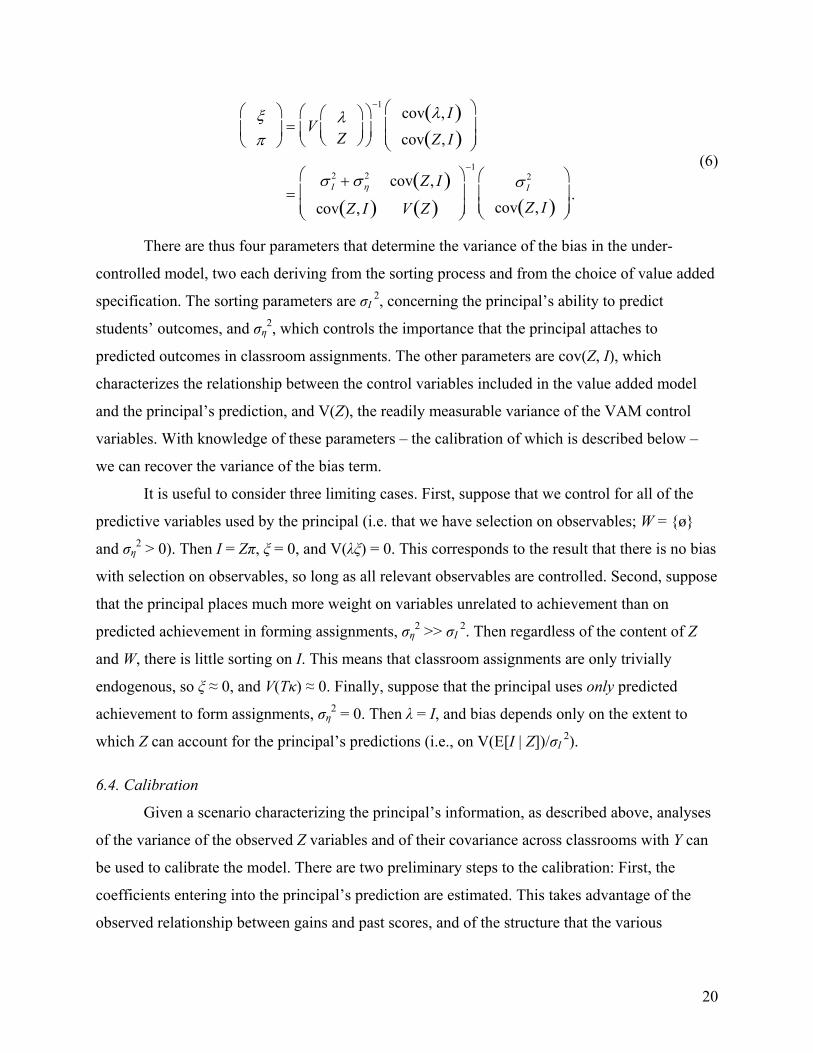
Moreover, recall that ξ and π are the coefficients from a regression of I onto λ and Z. Thus,
19 Things are somewhat more complex if classroom assignments are based on predictions of one outcome Y1 but another outcome Y2 is used as the dependent variable in the value added analysis. I set this issue aside for the moment. 20 Recall that I is an index formed from Z and W. Tκ thus represents the component of W that is correlated with T conditional on Z, while ν represents the component that cannot be predicted by {T, Z}.
19
(6)
ξπ
⎛
⎝⎜
⎞
⎠⎟ = V λ
Z⎛
⎝⎜⎞
⎠⎟⎛
⎝⎜
⎞
⎠⎟
−1cov λ, I( )cov Z, I( )
⎛
⎝⎜⎜
⎞
⎠⎟⎟
=σ I
2 + ση2 cov Z, I( )
cov Z, I( ) V Z( )
⎛
⎝⎜⎜
⎞
⎠⎟⎟
−1
σ I2
cov Z, I( )⎛
⎝⎜⎜
⎞
⎠⎟⎟
.
There are thus four parameters that determine the variance of the bias in the under-
controlled model, two each deriving from the sorting process and from the choice of value added
specification. The sorting parameters are σI 2, concerning the principal’s ability to predict
students’ outcomes, and ση2, which controls the importance that the principal attaches to
predicted outcomes in classroom assignments. The other parameters are cov(Z, I), which
characterizes the relationship between the control variables included in the value added model
and the principal’s prediction, and V(Z), the readily measurable variance of the VAM control
variables. With knowledge of these parameters – the calibration of which is described below –
we can recover the variance of the bias term.
It is useful to consider three limiting cases. First, suppose that we control for all of the
predictive variables used by the principal (i.e. that we have selection on observables; W = {ø}
and ση2 > 0). Then I = Zπ, ξ = 0, and V(λξ) = 0. This corresponds to the result that there is no bias
with selection on observables, so long as all relevant observables are controlled. Second, suppose
that the principal places much more weight on variables unrelated to achievement than on
predicted achievement in forming assignments, ση2 >> σI 2. Then regardless of the content of Z
and W, there is little sorting on I. This means that classroom assignments are only trivially
endogenous, so ξ ≈ 0, and V(Tκ) ≈ 0. Finally, suppose that the principal uses only predicted
achievement to form assignments, ση2 = 0. Then λ = I, and bias depends only on the extent to
which Z can account for the principal’s predictions (i.e., on V(E[I | Z])/σI 2).
6.4. Calibration
Given a scenario characterizing the principal’s information, as described above, analyses
of the variance of the observed Z variables and of their covariance across classrooms with Y can
be used to calibrate the model. There are two preliminary steps to the calibration: First, the
coefficients entering into the principal’s prediction are estimated. This takes advantage of the
observed relationship between gains and past scores, and of the structure that the various
20
scenarios place on the role of past scores in the principal’s predictions. Second, the degree of
sorting of students to classrooms is computed, using as an input the measured between-classroom
variance in observed predictor variables. The mechanics of each step are described in detail in
the appendix.
Once the parameters of the model are calibrated, the methods described in the previous
subsection can be used to compute the variance of the bias in a given value added model. I
consider value added models VAM2, VAM3, and VAM4 from Section 5. These are
distinguished by the control variables that are included in models for the grade-g gain. In each
case, the control variables are subsets of the A vector, so it is straightforward to compute the
covariance between these variables and the principal’s prediction. As indicated by equation (6),
this is sufficient to compute the variance of the bias term, V(Tκ).21
7. Results
7.1. The principal’s prediction
Table 2 presented prediction models for the 5th grade test score as a function of test
scores in earlier grades. As discussed above, these are readily converted into predictions of 5th
grade gains given the observed achievement history. Columns 1 and 2 of Table 7 present the
prediction coefficients when the predictor variables are the 4th grade reading score (column 1) or
the sequence of three prior reading scores (column 2). These correspond exactly to the
coefficients from columns 2 and 3 of Table 2 except that the 4th grade score coefficient is
reduced by one.
It may be that principals attempt to predict students’ true gains rather than their observed
gains. True gains are much harder to predict on the basis of past test scores. This is because the
noisy 4th grade test score achieves predictive power for the observed 5th grade gain due to the
presence of the same measurement error, u4, in both variables. Standard errors-in-variables
formulae (discussed in the Appendix) can be used to obtain the best prediction equations for true
gains. These are presented in columns 3 and 4 of Table 7.22 The within-school R2 statistics and
especially the prediction coefficients themselves are reduced in magnitude from the
21 Extending the analysis to VAMs that control for non-test variables requires assumptions about the relationship between these variables and the Z and W variables seen by the principal. I do not pursue this here. 22 In principle, the coefficients of regressions that include math scores could be recovered as well.
21
specifications for observed gains. True achievement gains are negatively correlated with past
achievement levels, but not dramatically so.23 The model for observed gains in column 2
implicitly attaches a coefficient of around -0.81 (= -0.57 − (-0.24)) to the 4th grade gain, while
the corresponding model for true gains assigns a weight of only -0.02 (= -0.07 − (-0.05)) to this
gain.
Table 8 presents estimates of the coefficients that the principal would apply to the
available predictor variables in scenarios C and D. Columns 1-4 show prediction coefficients for
observed gains, while columns 5-8 show coefficients for true gains. Columns 1 and 5 repeat the
coefficients from scenario B, where only the observed test score history is available. Columns 2
and 6 show coefficients when a second, equally noisy series is available. Columns 3 and 7 show
coefficients when two series are available in addition to observed scores (i.e. k = 2). Note that the
coefficients on the observed and unobserved series are identical in columns 6 and 7, where the
dependent variable is the true gain, but that they differ in columns 2 and 3, where the observed
series can be used to recover a portion of the measurement error in the observed gain. Columns 4
and 8 show predictions assuming that the principal is able to observe the history of true
achievement. This substantially improves his ability to predict observed gains, as the
measurement error portion of the 4th grade score can be perfectly isolated, but adds relatively
little to his ability to predict true gains over what could be done with three noisy histories. In
neither case is the coefficient on the 4th grade score equal to one. This implies (among other
things) that VAM2, which imposes a coefficient of 1 on the lagged achievement level, is mis-
specified.
7.2. The importance of predictions in classroom assignments
Using the coefficients from Tables 2, 7, and 8 and relying on an observed component of
the principal’s predictions, I can compute the variance decomposition of the principal’s
predictions, I, into within- and between-classroom components. For scenario C, I present
estimates for k = 1 and k = 2. In scenario E, I present estimates for f = 0.25, f = 0.5, and f = 1; the
scenario of perfect information, F, corresponds approximately to f = 1.96.
23 Note that the overall R2 statistics are higher in columns 3 and 4 than in 1 and 2, respectively. This is because the between-school component of observed achievement gains has very little measurement error in it. This means that a larger share of the variation of true gains than of observed gains is between schools, and also that the coefficients from within-school models for true gains are closer to the best prediction weights for across-school comparisons than are those from within-school models for observed gains.
22
The first column of Table 9 shows the fraction of the within-school variance in gains that
the principal is able to predict (i.e. σI 2/V(Y)) in each scenario, for true gains in the first panel and
for observed gains in the second panel. The second column shows the across-school share of
variance for the scenarios in which I is perfectly observable. Coefficients for between-school
predictions may differ from those for the within-school predictions that I focus on, so I do not
compute the across-school component of the incompletely observed indices. Column 3 shows the
fraction of the within-school variation that is across classrooms. This equals σI 2⁄(σI
2 + ση2), the
weight that the principal must be placing on predicted outcomes relative to other factors in
classroom assignments in order to generate the observed dispersion of past test scores across
classrooms. Column 4 shows the across-classroom standard deviation in predicted gains.
Not surprisingly, the scenarios in which the principal has more information permit him to
explain a larger share of the within-school variance in gains. Moreover, the richer prediction
scenarios yield larger estimates of the across-classroom share of variance of predicted gains.
Thus, the more information that we permit the principal to have about the student’s achievement
history, the larger is the bias that is implied for value added specifications (like VAM2) that do
not control for across-classroom sorting.
Sorting appears to be substantially more important when the principal is presumed to be
using predictions of observed rather than true gains for classroom assignments. But this can be
misleading: True gains are much less variable than observed gains (with a standard deviation less
than half as large). Disparities between the panels are smaller in Column 3, showing the fraction
of the variance of predicted gains that is across classrooms. Even in this column, though,
scenarios C-E show more sorting in the second panel. This is because observed scores form a
smaller share of predicted observed gains than of predicted true gains in these scenarios
(compare the R2 statistic in Column 1 of Table 8 to those in Columns 2-4, versus that in Column
5 and those in 6-8), so the same sorting on observed variables corresponds to more overall
sorting in the observed gain scenarios.
7.3. Bias in value added models with controls for observables
Table 9 shows that the standard deviation of across-classroom differences in predicted
gain scores ranges from 0.037 to 0.191, depending on the assumptions made about the
information used in sorting. This variation is bias in specifications like VAM2 that do not control
for classroom assignments. By comparison, the total across classroom standard deviation of
23
observed gain scores is 0.134. Thus, even scenarios that restrict the principal to use little more
than the observed variables in classroom assignments indicate biases in simple value added
models that are large relative to the effects that we hope to measure.
Table 10 presents estimates of the standard deviation of the bias in richer models that
include controls for students’ prior achievement. Columns 1-3 of this Table index value added
models, corresponding to VAM2, VAM3, and VAM4, respectively. The bias in the simplest
model (VAM2) is substantial in every scenario. Column 2 shows that the inclusion of a control
for the prior year’s test score eliminates much of the bias in VAM2, though there is important
variation across scenarios. If we assume that the principal forms classroom assignments on the
basis of his predictions of true gains (rather than observed gains) and that he has no information
about students’ potential gains beyond that contained in their achievement histories (as in
scenarios B-D), the remaining bias in VAM3 is negligible. However, if we allow the principal to
have additional information or if we assume that he sorts on the basis of predicted observed gains
– as he might under an accountability regime that conditions rewards and punishments on
observed gains rather than on unmeasurable true gains – then the bias remains important. If the
principal observes even two independent achievement histories (e.g. the test score history plus an
additional series, perhaps coming from teacher grades) and uses them in classroom assignments,
the standard deviation of the bias in VAM3 is 0.043.
Column 3 shows that much of the bias in VAM3 remains in VAM4, which controls for
the full sequence of prior test scores. If the principal is assumed to observe the student’s true
achievement history plus another set of variables that explain an equal amount of student gains
(i.e. scenario E with f = 1), the standard deviation of the bias ranges from 0.051 to 0.076, both
large relative to the standard deviation of teachers’ estimated “effects.”
8. Discussion
Typical value added analyses treat the process by which students are assigned to teachers
as ignorable, under the implicit assumption that the statistical model used can absorb any
systematic non-random assignment. This would be true if, for example, classroom assignments
were random conditional on students’ prior-grade test scores. But there is little reason to think
that this is an adequate characterization of classroom assignments. Principals have a great deal of
24
information beyond the prior test score that is predictive of students’ end-of-year achievement
and this information is unlikely to be ignored in classroom assignments.
This paper attempts to quantify the bias that arises in value added models that fail to
control for the determinants of classroom assignments. The task is straightforward if classroom
assignments are assumed to be random conditional on observable variables. My analysis
indicates that simple VAMs that fail to control for the dynamic process of test scores, simply
modeling differences in mean gain scores across classrooms, are substantially biased by student
sorting. The bias is reduced – with a variance about 15% as large as that of teachers’ true effects
– in a VAM that controls for the lagged score, and is further reduced when additional lagged
scores are included as controls. Of course, there are costs to this: The more past scores that are
required for the VAM estimation, the larger the share of students who will have to be excluded
from the analysis sample for reasons of missing data. Moreover, if three years of lagged scores
are needed for the VAM for 5th grade teachers, what is to be done about estimating the value
added of 3rd grade teachers, who see students before they have taken three years worth of tests?
The analysis is more complex if we loosen the unrealistic assumption that all of the
information considered by the principal in forming teacher assignments is available in the
research dataset. I develop methods for assessing the bias when the principal is assumed to have
access to a limited amount of information that the researcher cannot observe. I consider several
scenarios for the information set, and estimate the bias in three value added models under each
scenario.
A great deal turns out to depend on how the principal uses his information: If he weights
past achievement to best predict observed gains, even a limited amount of unobserved
information generates substantial biases in the sorts of value added models that are commonly
used. Richer models that control the full test score history rather than just a single lagged score
reduce these biases, but only if the principal has very limited information about students’
potential. With less restrictive assumptions, biases remain quantitatively important even in rich
value added models.
Of course, all of the analysis here (and in Rothstein (2008a, b), on which much of the
analysis in Section 4 is based) uses data on 5th graders in North Carolina. It is possible that the
results would differ in other data. This seems unlikely, however. Anecdotally, principals
everywhere are subject to pressure from parents seeking to manage their children’s classroom
25
assignments. The outcome of the resulting negotiations is unlikely to depend only on variables
that are observable in the data sets used for value added modeling. I therefore expect that the
results here would generalize to other states and school districts where student and teacher-level
accountability systems have low stakes, as in North Carolina in the period from which my data
were drawn.
Of more interest is the generalizability of my results to high-stakes settings. Any attempt
to predict the effect of adding stakes to the value added evaluation is necessarily speculative. But
it seems reasonable to guess that strong incentives attached to student scores or teacher value
added measures would strengthen the general results here. In a high stakes environment, teachers
would be wise to lobby principals for students who are predicted to post large gains in the
coming year, and principals would be tempted to use their control over classroom assignments to
reward favored teachers. In general, one would expect more sorting on the characteristics that
matter for the accountability system (i.e. lower ση2 in the model in Section 6) and therefore even
larger biases in the value added scores.
Three recent studies have provided evidence that appears to validate observational value-
added estimates. On closer examination, however, all are consistent with the presence of
substantial bias in these estimates. Jacob and Lefgren (2008) and Harris and Sass (2007)
compare value added estimates with principals’ subjective assessments of teacher quality, which
might be assumed to reflect unbiased estimates of teachers’ causal effects. Both papers find that
the two measures are correlated, though far from perfectly. This indicates that there is at least
some signal in the value added estimates. But the weak correlations leave plenty of room for
non-causal factors in the VAM estimates.
Kane and Staiger (2008) compare estimates of teacher effects from a randomized
experiment with observational estimates based on data prior to the experiment. They test the
hypothesis that the (appropriately shrunken) observational estimate is an unbiased prediction of
the causal estimate, and obtain estimates consistent with this hypothesis. There are three
important sources of slippage here, however. First, Kane and Staiger test a statistical hypothesis
about the joint distribution of the true coefficients and the bias; while zero bias is consistent with
the null hypothesis, so are large biases that are negatively correlated with teachers’ true causal
26
effects.24 Second, Kane and Staiger’s sample provides low power. Their standard errors are
consistent with substantial attenuation of the prediction coefficient due to bias in the
observational estimates. While their confidence intervals might rule out my scenario F (if biases
are assumed to be uncorrelated with true quality), my more realistic scenarios are wholly
consistent with the Kane and Staiger estimates but are nevertheless extremely troubling
regarding the potential for bias in value added estimates. Finally, the Kane and Staiger analysis is
based on a carefully selected sample of pairs of teachers for which principals consented to
random assignment. One might expect that principal consent was more likely when the two
teachers would have been given similar students in any case. If so, the results cannot be
generalized beyond the sample, even to other teachers at the same schools.
The results here suggest that it is hazardous to interpret typical value added estimates as
indicative of causal effects. Although some assumptions about the assignment process permit
nearly unbiased estimation, other plausible assumptions yield large biases. Further evidence on
the process by which students are assigned to classrooms is needed before it will be clear which
types of assumptions are closest to reality. The most recent such study, Monk (1987), is now
more than twenty years old. More recent evidence, from studies more directly targeted at the
assumptions of value added modeling, is badly needed, as are richer VAMs that can account for
real world assignments. In the meantime, causal claims will be tenuous at best.
24 They test the hypothesis that cov(β, κ)/V(κ) = 1, where β is the vector of causal effects and κ is the best linear predictor of b, the sum of causal effects and any sorting bias, based on the coefficients from the value added model. This equality will hold either if V(b – β) = 0 – i.e., there is no bias – or if corr (β, b – β) = − V b − β( ) V β( ) .
27
References
Aaronson, Daniel, Lisa Barrow, and William Sander. 2007. Teachers and Student Achievement in the Chicago Public High Schools. Journal of Labor Economics 24 (1): 95–135.
Altonji, Joseph G., Todd E. Elder, and Christopher R. Taber. 2005. Selection on observed and unobserved variables: Assessing the effectiveness of Catholic schools. Journal of Political Economy 113 (1): 151–184.
Ballou, Dale. 2002. Sizing up test scores. Education Next 2 (2): 10–15.
Bazemore, Mildred. 2004. North Carolina reading comprehension tests. Technical report (citable draft), Office of Curriculum and School Reform Services, North Carolina Department of Public Instruction.
Boyd, Donald, Hamilton Lankford, Susanna Loeb, Jonah Rockoff, and James Wyckoff. 2008. The narrowing gap in New York City teacher qualifications and its implications for student achievement in high-poverty schools. Journal of Policy Analysis and Management 27 (4): 793–818.
Clotfelter, Charles T., Helen F. Ladd, and Jacob L. Vigdor. 2006. Teacher-student matching and the assessment of teacher effectiveness. Journal of Human Resources 41 (4): 778–820.
Goldhaber, Dan. 2007. Everyone’s doing it, but what does teacher testing tell us about teacher effectiveness? Journal of Human Resources 42 (4): 765–794.
Gordon, Robert, Thomas J. Kane, and Douglas O. Staiger. 2006. Identifying effective teachers using performance on the job. Hamilton Project Discussion Paper No. 2006-01.
Harris, Douglas N., and Tim R. Sass. 2006. Value-added models and the measurement of teacher quality. Unpublished paper, Florida State University.
Harris, Douglas N., and Tim R. Sass. 2007. What makes for a good teacher and who can tell? Unpublished paper, Florida State University.
Jacob, Brian A., and Lars Lefgren. 2008. Can principals identify effective teachers? Evidence on subjective performance evaluation in education. Journal of Labor Economics 25 (1): 101–136.
Kane, Thomas J., and Douglas O. Staiger. 2008. Estimating teacher impacts on student achievement: An experimental evaluation. NBER Working Paper No. 14607
Kane, Thomas J., Jonah E. Rockoff, and Douglas O. Staiger. 2008. What does certification tell us about teacher effectiveness? Evidence from New York City. Economics of Education Review 27 (6): 615–631.
28
Koedel, Cory, and Julian R. Betts. 2007. Re-examining the role of teacher quality in the educational production function. Working paper 07-08, University of Missouri Department of Economics April.
Martineau, Joseph A. 2006. Distorting value added: The use of longitudinal, vertically scaled student achievement data for growth-based, value-added accountability. Journal of Educational and Behavioral Statistics 31 (1): 35–62.
Monk, David H. 1987. Assigning elementary pupils to their teachers. Elementary School Journal 88 (2): 167–187.
Rivkin, Steven G., Eric A. Hanushek, and John F. Kain. 2005. Teachers, schools, and academic achievement. Econometrica 73 (2): 417–458.
Rothstein, Jesse. 2008a. Teacher quality in educational production: Tracking, decay, and student achievement. Princeton University Education Research Section Working Paper No. 25.
Rothstein, Jesse. 2008b. Teacher quality in educational production: Tracking, decay, and student achievement. NBER Working Paper No. 14442.
Sanders,William L., and Sandra P. Horn. 1994. The Tennessee value-added assessment system (TVAAS): Mixed-model methodology in educational assessment. Journal of Personnel Evaluation in Education 8 (3): 299–311.
Sanders,William L., Arnold M. Saxton, and Sandra P. Horn. 1997. The Tennessee value-added assessment system: A quantitative, outcomes-based approach to educational assessment. In Grading teachers, grading schools: Is student achievement a valid evaluation measure?, edited by Jason Millman, pp 137-162. Thousand Oaks, CA: Corwin.
Sanford, Eleanor E. 1996. North Carolina end-of-grade tests: reading comprehension, mathematics. Technical report No. 1, Division of Accountability/Testing, Office of Instructional and Accountability Services, North Carolina Department of Public Instruction.
Yen, Wendy. 1986. The choice of scale for educational measurement: An IRT perspective. Journal of Educational Measurement 23 (4): 299–325.
29
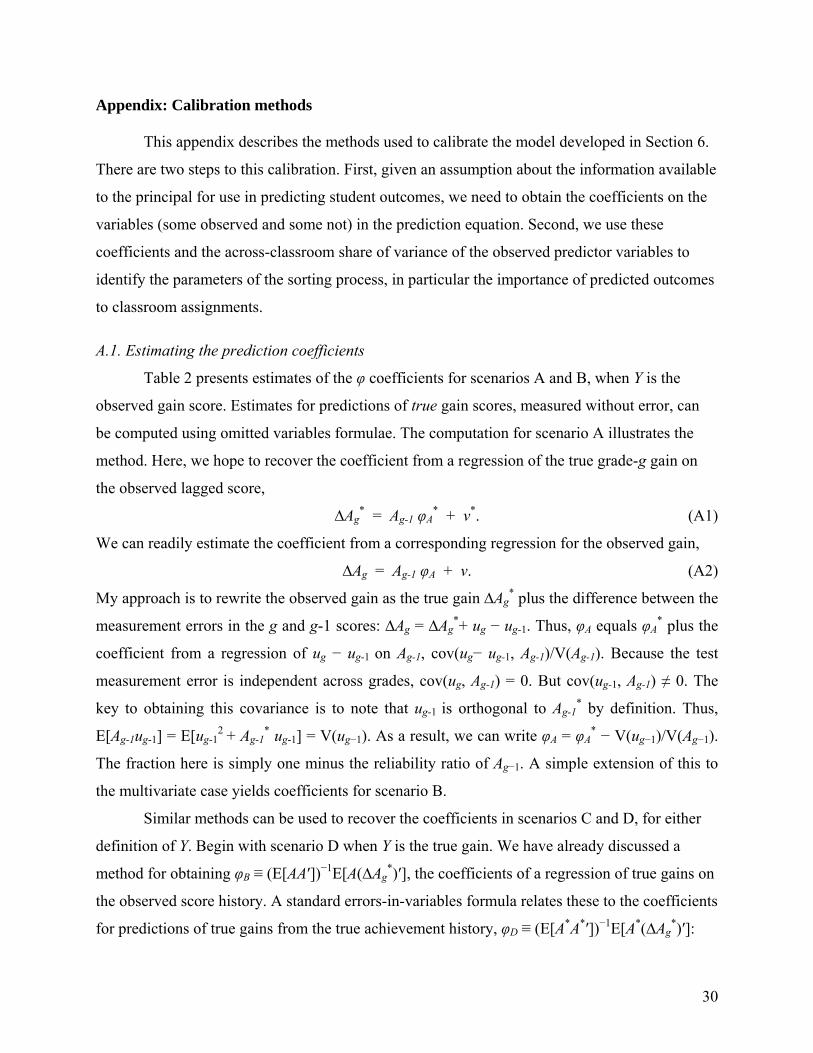
Appendix: Calibration methods
This appendix describes the methods used to calibrate the model developed in Section 6.
There are two steps to this calibration. First, given an assumption about the information available
to the principal for use in predicting student outcomes, we need to obtain the coefficients on the
variables (some observed and some not) in the prediction equation. Second, we use these
coefficients and the across-classroom share of variance of the observed predictor variables to
identify the parameters of the sorting process, in particular the importance of predicted outcomes
to classroom assignments.
A.1. Estimating the prediction coefficients
Table 2 presents estimates of the φ coefficients for scenarios A and B, when Y is the
observed gain score. Estimates for predictions of true gain scores, measured without error, can
be computed using omitted variables formulae. The computation for scenario A illustrates the
method. Here, we hope to recover the coefficient from a regression of the true grade-g gain on
the observed lagged score,
∆Ag* = Ag-1 φA
* + v*. (A1)
We can readily estimate the coefficient from a corresponding regression for the observed gain,
∆Ag = Ag-1 φA + v. (A2)
My approach is to rewrite the observed gain as the true gain ∆Ag* plus the difference between the
measurement errors in the g and g-1 scores: ∆Ag = ∆Ag*+ ug − ug-1. Thus, φA equals φA
* plus the
coefficient from a regression of ug − ug-1 on Ag-1, cov(ug− ug-1, Ag-1)/V(Ag-1). Because the test
measurement error is independent across grades, cov(ug, Ag-1) = 0. But cov(ug-1, Ag-1) ≠ 0. The
key to obtaining this covariance is to note that ug-1 is orthogonal to Ag-1* by definition. Thus,
E[Ag-1ug-1] = E[ug-12 + Ag-1
* ug-1] = V(ug−1). As a result, we can write φA = φA* − V(ug−1)/V(Ag−1).
The fraction here is simply one minus the reliability ratio of Ag−1. A simple extension of this to
the multivariate case yields coefficients for scenario B.
Similar methods can be used to recover the coefficients in scenarios C and D, for either
definition of Y. Begin with scenario D when Y is the true gain. We have already discussed a
method for obtaining φB ≡ (E[AA′])−1E[A(∆Ag*)′], the coefficients of a regression of true gains on
the observed score history. A standard errors-in-variables formula relates these to the coefficients
for predictions of true gains from the true achievement history, φD ≡ (E[A*A*′])−1E[A*(∆Ag*)′]:
30
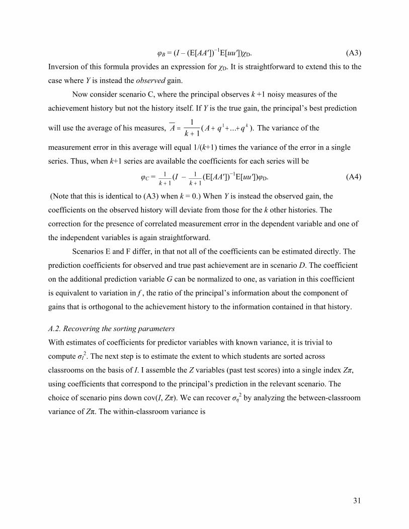
φB = (I – (E[AA′])−1E[uu′])χD. (A3)
Inversion of this formula provides an expression for χD. It is straightforward to extend this to the
case where Y is instead the observed gain.
Now consider scenario C, where the principal observes k +1 noisy measures of the
achievement history but not the history itself. If Y is the true gain, the principal’s best prediction
will use the average of his measures, Ak
A q q k=+
+ + +1
11( ... ). The variance of the
measurement error in this average will equal 1/(k+1) times the variance of the error in a single
series. Thus, when k+1 series are available the coefficients for each series will be
φC = 11k +
(I – 11k +
(E[AA′])−1E[uu′])φD. (A4)
(Note that this is identical to (A3) when k = 0.) When Y is instead the observed gain, the
coefficients on the observed history will deviate from those for the k other histories. The
correction for the presence of correlated measurement error in the dependent variable and one of
the independent variables is again straightforward.
Scenarios E and F differ, in that not all of the coefficients can be estimated directly. The
prediction coefficients for observed and true past achievement are in scenario D. The coefficient
on the additional prediction variable G can be normalized to one, as variation in this coefficient
is equivalent to variation in f , the ratio of the principal’s information about the component of
gains that is orthogonal to the achievement history to the information contained in that history.
A.2. Recovering the sorting parameters
With estimates of coefficients for predictor variables with known variance, it is trivial to
compute σI2. The next step is to estimate the extent to which students are sorted across
classrooms on the basis of I. I assemble the Z variables (past test scores) into a single index Zπ,
using coefficients that correspond to the principal’s prediction in the relevant scenario. The
choice of scenario pins down cov(I, Zπ). We can recover ση2 by analyzing the between-classroom
variance of Zπ. The within-classroom variance is
31
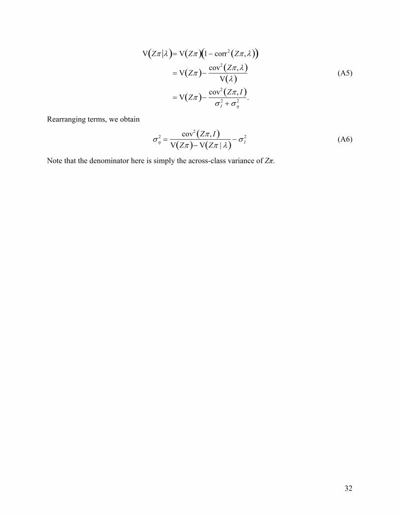
V Zπ λ( )= V Zπ( ) 1− corr2 Zπ ,λ( )( )= V Zπ( )− cov2 Zπ ,λ( )
V λ( )
= V Zπ( )− cov2 Zπ , I( )σ I
2 + ση2 .
(A5)
Rearranging terms, we obtain
ση2 =
cov2 Zπ , I( )V Zπ( )− V Zπ | λ( )
− σ I2 (A6)
Note that the denominator here is simply the across-class variance of Zπ.
32
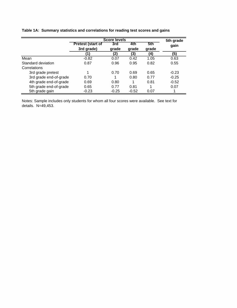
Table 1A: Summary statistics and correlations for reading test scores and gains
Pretest (start of 3rd grade)
3rd grade
4th grade
5th grade
(1) (2) (3) (4) (5)Mean -0.82 0.07 0.42 1.05 0.63Standard deviation 0.87 0.96 0.95 0.82 0.55Correlations
3rd grade pretest 1 0.70 0.69 0.65 -0.233rd grade end-of-grade 0.70 1 0.80 0.77 -0.254th grade end-of-grade 0.69 0.80 1 0.81 -0.525th grade end-of-grade 0.65 0.77 0.81 1 0.075th grade gain -0.23 -0.25 -0.52 0.07 1
Score levels 5th grade gain
Notes: Sample includes only students for whom all four scores were available. See text for details. N=49,453.
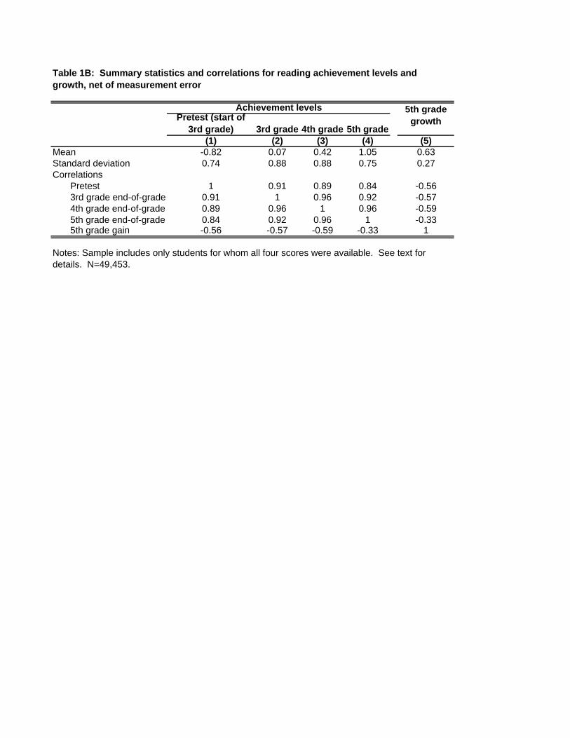
Pretest (start of 3rd grade) 3rd grade 4th grade 5th grade
(1) (2) (3) (4) (5)Mean -0.82 0.07 0.42 1.05 0.63Standard deviation 0.74 0.88 0.88 0.75 0.27Correlations
Pretest 1 0.91 0.89 0.84 -0.563rd grade end-of-grade 0.91 1 0.96 0.92 -0.574th grade end-of-grade 0.89 0.96 1 0.96 -0.595th grade end-of-grade 0.84 0.92 0.96 1 -0.335th grade gain -0.56 -0.57 -0.59 -0.33 1
Achievement levels 5th grade growth
Table 1B: Summary statistics and correlations for reading achievement levels and growth, net of measurement error
Notes: Sample includes only students for whom all four scores were available. See text for details. N=49,453.
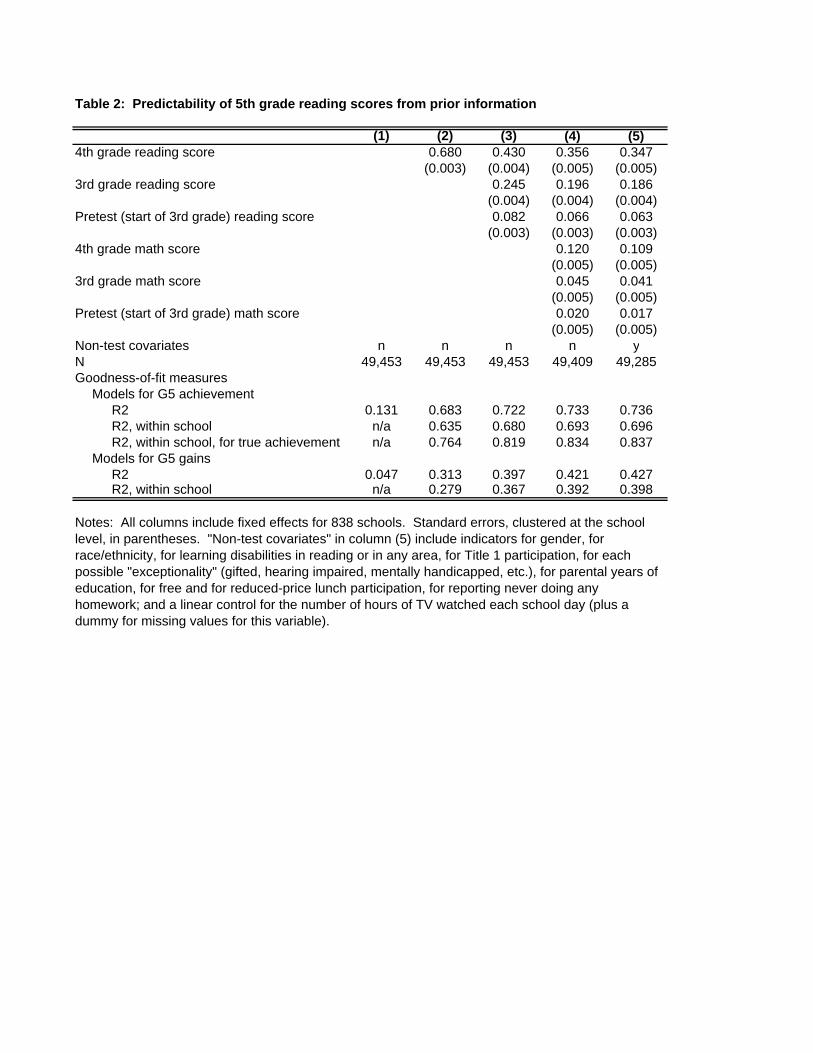
Table 2: Predictability of 5th grade reading scores from prior information
(1) (2) (3) (4) (5)4th grade reading score 0.680 0.430 0.356 0.347
(0.003) (0.004) (0.005) (0.005)3rd grade reading score 0.245 0.196 0.186
(0.004) (0.004) (0.004)Pretest (start of 3rd grade) reading score 0.082 0.066 0.063
(0.003) (0.003) (0.003)4th grade math score 0.120 0.109
(0.005) (0.005)3rd grade math score 0.045 0.041
(0.005) (0.005)Pretest (start of 3rd grade) math score 0.020 0.017
(0.005) (0.005)Non-test covariates n n n n yN 49,453 49,453 49,453 49,409 49,285Goodness-of-fit measures
Models for G5 achievementR2 0.131 0.683 0.722 0.733 0.736R2, within school n/a 0.635 0.680 0.693 0.696R2, within school, for true achievement n/a 0.764 0.819 0.834 0.837
Models for G5 gainsR2 0.047 0.313 0.397 0.421 0.427R2, within school n/a 0.279 0.367 0.392 0.398
Notes: All columns include fixed effects for 838 schools. Standard errors, clustered at the school level, in parentheses. "Non-test covariates" in column (5) include indicators for gender, for race/ethnicity, for learning disabilities in reading or in any area, for Title 1 participation, for each possible "exceptionality" (gifted, hearing impaired, mentally handicapped, etc.), for parental years of education, for free and for reduced-price lunch participation, for reporting never doing any homework; and a linear control for the number of hours of TV watched each school day (plus a dummy for missing values for this variable).
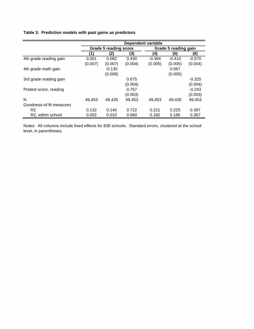
Table 3: Prediction models with past gains as predictors
(1) (2) (3) (4) (5) (6)4th grade reading gain 0.051 0.082 0.430 -0.394 -0.410 -0.570
(0.007) (0.007) (0.004) (0.005) (0.005) (0.004)4th grade math gain -0.130 0.067
(0.008) (0.005)3rd grade reading gain 0.675 -0.325
(0.004) (0.004)Pretest score, reading 0.757 -0.243
(0.003) (0.003)N 49,453 49,435 49,453 49,453 49,435 49,453Goodness-of-fit measures
R2 0.132 0.140 0.722 0.221 0.225 0.397R2, within school 0.002 0.010 0.680 0.182 0.186 0.367
Grade 5 reading score Grade 5 reading gainDependent variable
Notes: All columns include fixed effects for 838 schools. Standard errors, clustered at the school level, in parentheses.
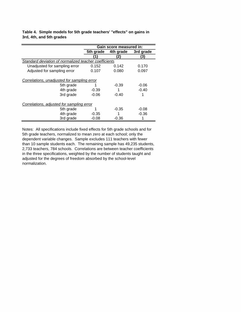
5th grade 4th grade 3rd grade(1) (2) (3)
Standard deviation of normalized teacher coefficientsUnadjusted for sampling error 0.152 0.142 0.170Adjusted for sampling error 0.107 0.080 0.097
Correlations, unadjusted for sampling error5th grade 1 -0.39 -0.064th grade -0.39 1 -0.403rd grade -0.06 -0.40 1
Correlations, adjusted for sampling error5th grade 1 -0.35 -0.084th grade -0.35 1 -0.363rd grade -0.08 -0.36 1
Gain score measured in:
Table 4. Simple models for 5th grade teachers' "effects" on gains in 3rd, 4th, and 5th grades
Notes: All specifications include fixed effects for 5th grade schools and for 5th grade teachers, normalized to mean zero at each school; only the dependent variable changes. Sample excludes 111 teachers with fewer than 10 sample students each. The remaining sample has 49,235 students, 2,733 teachers, 784 schools. Correlations are between teacher coefficients in the three specifications, weighted by the number of students taught and adjusted for the degrees of freedom absorbed by the school-level normalization.
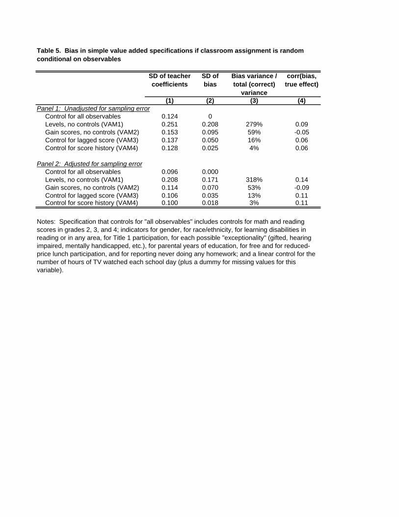
SD of teacher coefficients
SD of bias
Bias variance / total (correct)
variance
corr(bias, true effect)
(1) (2) (3) (4)Panel 1: Unadjusted for sampling error
Control for all observables 0.124 0Levels, no controls (VAM1) 0.251 0.208 279% 0.09Gain scores, no controls (VAM2) 0.153 0.095 59% -0.05Control for lagged score (VAM3) 0.137 0.050 16% 0.06Control for score history (VAM4) 0.128 0.025 4% 0.06
Panel 2: Adjusted for sampling errorControl for all observables 0.096 0.000Levels, no controls (VAM1) 0.208 0.171 318% 0.14Gain scores, no controls (VAM2) 0.114 0.070 53% -0.09Control for lagged score (VAM3) 0.106 0.035 13% 0.11Control for score history (VAM4) 0.100 0.018 3% 0.11
Notes: Specification that controls for "all observables" includes controls for math and reading scores in grades 2, 3, and 4; indicators for gender, for race/ethnicity, for learning disabilities in reading or in any area, for Title 1 participation, for each possible "exceptionality" (gifted, hearing impaired, mentally handicapped, etc.), for parental years of education, for free and for reduced-price lunch participation, and for reporting never doing any homework; and a linear control for the number of hours of TV watched each school day (plus a dummy for missing values for this variable).
Table 5. Bias in simple value added specifications if classroom assignment is random conditional on observables
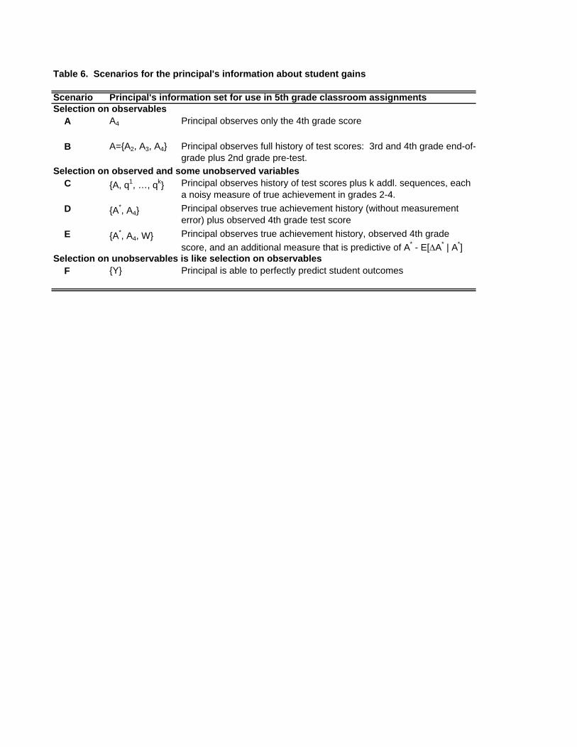
Table 6. Scenarios for the principal's information about student gains
Scenario Principal's information set for use in 5th grade classroom assignmentsSelection on observables
A A4 Principal observes only the 4th grade score
B A={A2, A3, A4} Principal observes full history of test scores: 3rd and 4th grade end-of-grade plus 2nd grade pre-test.
C {A, q1, …, qk} Principal observes history of test scores plus k addl. sequences, each a noisy measure of true achievement in grades 2-4.
D {A*, A4} Principal observes true achievement history (without measurement error) plus observed 4th grade test score
E {A*, A4, W} Principal observes true achievement history, observed 4th grade score, and an additional measure that is predictive of A* - E[ΔA* | A*]
F {Y} Principal is able to perfectly predict student outcomes
Selection on observed and some unobserved variables
Selection on unobservables is like selection on observables
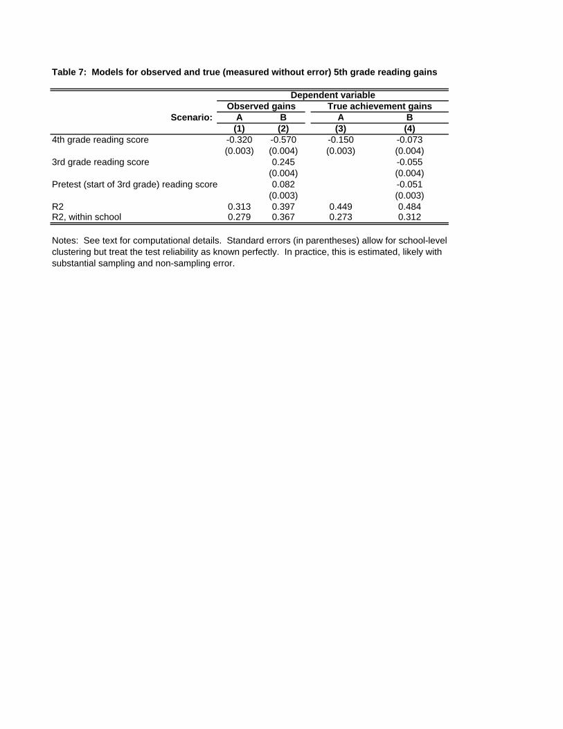
Table 7: Models for observed and true (measured without error) 5th grade reading gains
Scenario: A B A B(1) (2) (3) (4)
4th grade reading score -0.320 -0.570 -0.150 -0.073(0.003) (0.004) (0.003) (0.004)
3rd grade reading score 0.245 -0.055(0.004) (0.004)
Pretest (start of 3rd grade) reading score 0.082 -0.051(0.003) (0.003)
R2 0.313 0.397 0.449 0.484R2, within school 0.279 0.367 0.273 0.312
Notes: See text for computational details. Standard errors (in parentheses) allow for school-level clustering but treat the test reliability as known perfectly. In practice, this is estimated, likely with substantial sampling and non-sampling error.
Observed gains True achievement gainsDependent variable
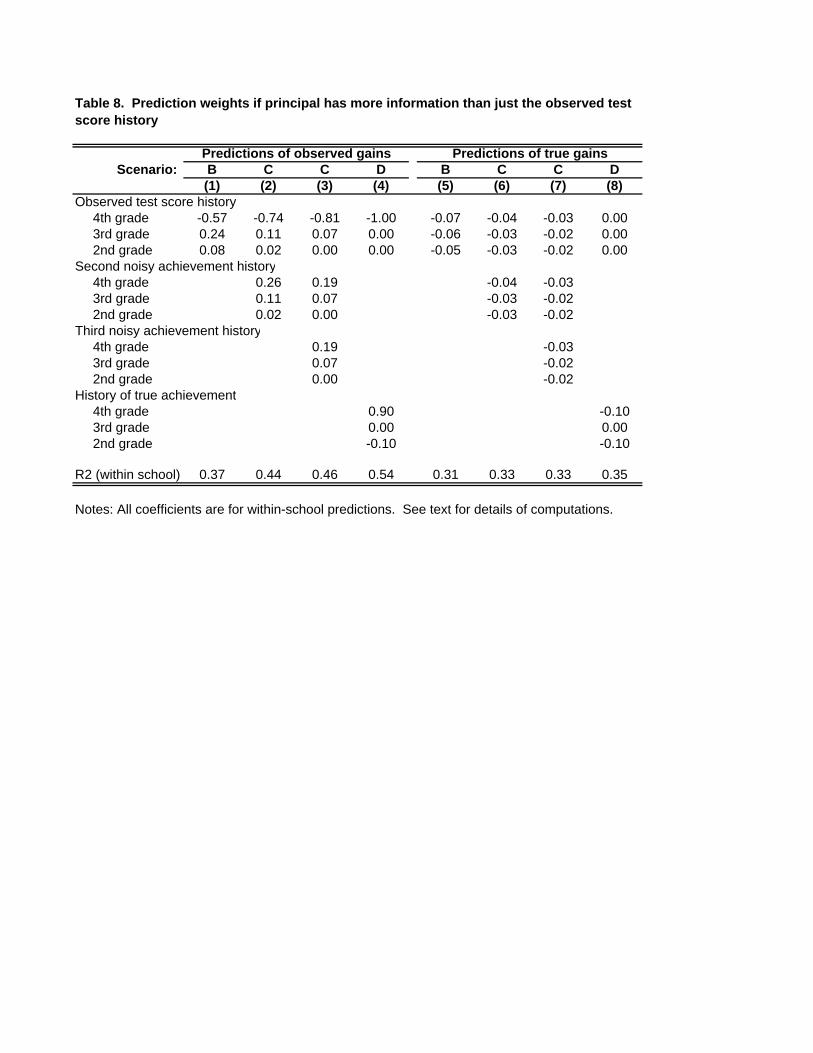
Scenario: B C C D B C C D(1) (2) (3) (4) (5) (6) (7) (8)
Observed test score history4th grade -0.57 -0.74 -0.81 -1.00 -0.07 -0.04 -0.03 0.003rd grade 0.24 0.11 0.07 0.00 -0.06 -0.03 -0.02 0.002nd grade 0.08 0.02 0.00 0.00 -0.05 -0.03 -0.02 0.00
Second noisy achievement history4th grade 0.26 0.19 -0.04 -0.033rd grade 0.11 0.07 -0.03 -0.022nd grade 0.02 0.00 -0.03 -0.02
Third noisy achievement history4th grade 0.19 -0.033rd grade 0.07 -0.022nd grade 0.00 -0.02
History of true achievement4th grade 0.90 -0.103rd grade 0.00 0.002nd grade -0.10 -0.10
R2 (within school) 0.37 0.44 0.46 0.54 0.31 0.33 0.33 0.35
Notes: All coefficients are for within-school predictions. See text for details of computations.
Predictions of observed gains Predictions of true gains
Table 8. Prediction weights if principal has more information than just the observed test score history
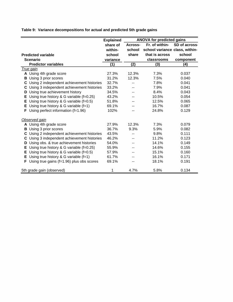
Table 9: Variance decompositions for actual and predicted 5th grade gains
Predicted variableScenario
Predictor variables (1) (2) (3) (4)True gain
A Using 4th grade score 27.3% 12.3% 7.3% 0.037B Using 3 prior scores 31.2% 12.3% 7.5% 0.040C Using 2 independent achievement histories 32.7% -- 7.8% 0.041C Using 3 independent achievement histories 33.2% -- 7.9% 0.041D Using true achievement history 34.5% -- 8.4% 0.043E Using true history & G variable (f=0.25) 43.2% -- 10.5% 0.054E Using true history & G variable (f=0.5) 51.8% -- 12.5% 0.065E Using true history & G variable (f=1) 69.1% -- 16.7% 0.087F Using perfect information (f=1.96) 102% -- 24.8% 0.129
Observed gainA Using 4th grade score 27.9% 12.3% 7.3% 0.079B Using 3 prior scores 36.7% 9.3% 5.9% 0.082C Using 2 independent achievement histories 43.5% -- 9.8% 0.111C Using 3 independent achievement histories 46.2% -- 11.2% 0.123D Using obs. & true achievement histories 54.0% -- 14.1% 0.149E Using true history & G variable (f=0.25) 55.9% -- 14.6% 0.155E Using true history & G variable (f=0.5) 57.9% -- 15.1% 0.160E Using true history & G variable (f=1) 61.7% -- 16.1% 0.171F Using true gains (f=1.96) plus obs scores 69.1% -- 18.1% 0.191
5th grade gain (observed) 1 4.7% 5.8% 0.134
Explained share of within-school
variance
ANOVA for predicted gainsAcross-school share
Fr. of within-school variance
that is across classrooms
SD of across-class, within-
school component
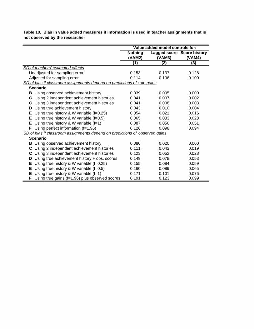
Nothing Lagged score Score history(VAM2) (VAM3) (VAM4)
(1) (2) (3)SD of teachers' estimated effects
Unadjusted for sampling error 0.153 0.137 0.128Adjusted for sampling error 0.114 0.106 0.100
SD of bias if classroom assignments depend on predictions of true gainsScenarioB Using observed achievement history 0.039 0.005 0.000C Using 2 independent achievement histories 0.041 0.007 0.002C Using 3 independent achievement histories 0.041 0.008 0.003D Using true achievement history 0.043 0.010 0.004E Using true history & W variable (f=0.25) 0.054 0.021 0.016E Using true history & W variable (f=0.5) 0.065 0.033 0.028E Using true history & W variable (f=1) 0.087 0.056 0.051F Using perfect information (f=1.96) 0.126 0.098 0.094
SD of bias if classroom assignments depend on predictions of observed gainsScenarioB Using observed achievement history 0.080 0.020 0.000C Using 2 independent achievement histories 0.111 0.043 0.019C Using 3 independent achievement histories 0.123 0.052 0.028D Using true achievement history + obs. scores 0.149 0.078 0.053E Using true history & W variable (f=0.25) 0.155 0.084 0.059E Using true history & W variable (f=0.5) 0.160 0.089 0.065E Using true history & W variable (f=1) 0.171 0.101 0.076F Using true gains (f=1.96) plus observed scores 0.191 0.123 0.099
Table 10. Bias in value added measures if information is used in teacher assignments that is not observed by the researcher
Value added model controls for: