STUDIA GEOBOTANICA

o: 140-165. 198ii

THE USE OF ELLIPSES OF EQUAL CONCENTRATION TO ANALYSE ORDINATION VEGETATION PATTERNS

Mario LAGONEGRO and Enrico FEOLI

Keywords: Ellipses, Forest, Ordination, Pattern, Structure.

Abstract: The use of ellipses of equa! concentration is suggested for the analysis of pattern in ordination scattergrams produced directly by environmental variables, or with axes obtained by numerica! methods. The potentials of the method are illustrated by some examples using structural characteristics of mixed forest type of NE Italy and environmental variables estimated by ecologica! indica tor values.

Introduction

The analysis of vegetation patterns detected by ordination scattergrams can be clone by the method suggested by Feoli & Ganis (1986). It consists in the use of a revised version of the Moran formula (Cliff & Ord, 1981) of autocorrelation for testing if the values of a variable, simple or composite, have a non-random pattern in the spaces defined by other ecological variables. The method does not give any information about the barycentre of the variable or about the correlation between the variables which define the space. We think that the method of ellipses of egual concentration (see Daboni, 1967; Mardia, Kent & Bibby, 1979) should constitute a further extension of the autocorrelation method in describing vegetation pattern relateci to ordination scattergrams.

The method

Given N points with coordinates (x i• y) for i = 1, ... , N, with which are associateci N scores (p) of a variable i, the coordinates of the barycentre of the variable i in the space defined by the axes x and y are:

N N

Xc = -1- L · p · x

T I' ' '

Yc = -1

L P·Y·T 1' ' '

N

where T = L; p; . The parameters of dispersion of x and y around the barycentreI

are:

143

Sxy =

s 2 =X

s � = � i ( � ) (y i - y a> 2

� . ( _____f!J__ ) I' T

R=

R is the correlation coefficient. One can define the ellipse of egual concentration k as:

RI "'l'=l

which is centered at (X e, Y a) with axes and inclination defined by s ! s ! R. It corresponds to the curve which, on the (x, y) plane, given a binormal distributionhaving the maximum at the barycentre, leaves outside itself a residual egual to exp (-k) (tail probability). It must be remembered that the total amounts to unity. It follows that if one wants an ellipse excluding 5 % of the total binormal distribution, Kmust be estimated as:

5 e-k = -- = 0.05

100

k = - ln 0.05

In general if a percentage P is to be excluded:

The corresponding ellipse will satisfy the following relation:

144

( x-X0)2_ 2R(

x-X 0

sx sx

If

then:

Y - y G ) + ( Y - y G ) 2 = k p (1 _ R 2)

Sy Sy

y- Yay s =

-"------=-

by reordering and taking X 8 as an independent variable

a Yi + b Y s + e = O

where:

a = l b=-2RX8 e = Xi - kp (1 - R2)

the solutions are real if:

b2

- 4 a e 2: O

it follows that values of X 8 may be derived from:

(Xi - kJ (1 - R 2) = O

since - 1 < R < 1 and consequently (1 - R2) � O

it follows that:

an in consequence

The parameters computed in this way are used to compute the y values and to

draw the ellipses.

When more than one group of objects is considered, or when a group is

145

considered under different weighting approaches, the ellipses can be computed for each group. The differences between the groups may be tested by Student' s estimated as follows:

where:

t = _D_[ _ [ M N

J 112

S 12 M+N

D =

[ (X c1 - X cJ 2 + (Y c1 - y cJ

2

J 112

S = [ (N - 1) s � + (M - 1) s �

] 112 12 M+N-2

N being the number of objects in group 1, M that of group 2. The program also computes the regression lines for each group and tests for

differences between the population slopes and intercepts, two by two, (Zar, 197 4). The formulae are: for slopes

t =

s2 +

s2 --�-Jil2

N N N M M M

[ L;y;-(L;x;yJ/L;xU+[L;y;-(L;x;yJ/L1

; x�J I I I 1 I s2 =-------------------------

xy

N+M-4

for elevations

146

N M

( ;;x;y)+(;; X;Y) ac = -----------

M

The program ELLIPLOT (1), written both in GW-BASIC and FORTRAN 77 for personal computers operating under MS-DOS, is listed in the Appendix.

Examples

The method has been applied to data of mixed forest types obtained by Lagonegro and Feoli (1985) from Poldini (1982). They consist of two matrices describing 20 vegetation forest types. In one matrix the description of the types is based on the combination of life forms and growth forms (life-growth forms); in the other it is based on the average indicator values, Landolt (1977). The method of ranking characters proposed by Orl6ci (1973) has been applied to the matrices, in order to select variables for the examples.

In the first place, the environmental variables as indicateci by the average indicator values of the species were used as axes.

Among the environmental variables, humidity, temperature and pH have been chosen because they explain more than 90% of the total sum of squares. These variables, two at a time, served as axes to test for the pattern of all the life-growth forms. Among those with significant patterns (according to the autocorrelation method), we used those accounting for more than 90% of total sum of squares. They are: scapose hemicryptophytes, rhizome geophytes and suffrutescent chamae­phytes.

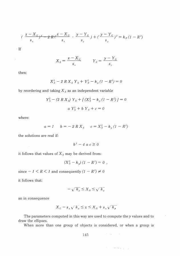
In Figure 1 (a, b) is given an example of output of the program ELLIPLOT applied to the ordination scattergram with humidity and pH as axes, using the values of suffrutescent chamaephytes. Figure la shows the barycentre of the life­growth form in the space defined by humidity and pH, and the ellipses cor­responding to 0.1, 1, 5, 31. 7 percent tail probability. The regression line of the two variables is also printed.

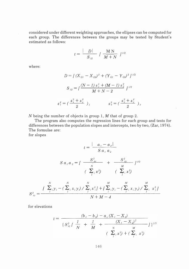
Figure 1 b shows the centroid of the two variables. The program also provides for the two figures to be drawn both on a graph as in Figure 2. In this case only two ellipses are drawn (those at 5% probability) to avoid excessive complexity.

The deviation of the centroid from the barycentre may be used as a measure of asymmetry of the pattern of the life-growth form with respect to the two variables · used as ordination axes. The t test, estimated as described above, can serve as sucha measure. In the case of Figure 2 the deviation of the barycentre from the centroid

(1) The program is included in a library (47 programs) written in GW-BASIC for persona! computersrunning under MS-DOS operating system (Lagonegro & Feoli, 1985).

147

a ----· .-----. -----

11/' ··-. ·······--.....

. ··

···-···

·

.-·----.,

····-... \···....... / ··--... ___ ·· .. ,

\ • •• I

(

•• •••

•

•• •••••••••

··, ••••• •.•••••••

, .

�

I _.- --------..... ______ ·-•.

\, .. , \ . ·--,_ ., __\ '., ·---.. _

', \, "'·-.... _ (.-------. ___ _ \ t-.... I ··.,. . ..I. ... ·-., ..

· .......

•· ', '

',\ ··········,..

....... ..········:···· .... �

·· ...

.

... .

'··· .....

. �

�\\ ··, .. ,�- . , ·. I"-.. , ······ ...

·· ...•..I

\

.\\ · ...

.

... �· \,

.. \\ ·· ... \.

, . ····-.

:1 .. '· \,

.............. ·······-·--·--'

° \ \. '·

···-... �Il \\""· .....

\ .• --

.. ····---... _ -

"•.. -.,.,_ Il Il \"• •• ··•. ·-.. ··-...... .. I ,, '\, ·--. ______ , __ ./

11

101

·------. -... ,_ ___ ... I I ··· ............. !�.��-··-··-·--······ .. / il

····-. ___________ ..• -"/

•

Fig. 1 (a) - Ellipses of equa! concentration drawn at probability levels of0.317, 0.05, 0.01 and 0.001 with reference to the barycentre of suffrutescent chamaephytes.

is significant t - p< 2% .. This proves that the suffrutescent chamaephytes have a pattern that is asymmetric with respect to the centroid of the two variables .. This does not happen for the other two life.growth forms ..

The ellipses are useful in quantifying the pattern of a variable in ordination scattergrams .. The pattern may be described by the cumulative frequencies of the points included in the ellipses corresponding to different probability levels, as in Table 1. The deviations from the expected frequencies, which can be calculated by multiplying the expected cumulative probability values by the total number of objects in the scattergram, may be used in a chi square test .. From Table 1 one can conclude that the pattern deviating most from that expected is that of suffrutescent

148

_ ... ----"" ............ � ..

b

-·· ·-· ·· 1

I I I I

i

'----------------------·-··----.. ·····-·-------

Fig. 1 (b) - Ellipses of equa! concentration drawn at probability levels of0.317, 0.05, 0.01 and 0.001 with reference to the centròid of the two variables defining the space: humidity and pH.

chamaephytes, followed by that of scapose hemicryptophytes. The pattern for rhizome geophytes does not deviate significantly from that expected. If one considers the two main groups of communities defined by the dendrogram of Figure 7 in Lago negro & Feoli (1985), then one can see from Figure 3 that for cluster a there is no deviation from expectation, while for cluster b there is a significant deviation. This means that the cluster a represents a homogeneous environment for the suffrutescent chamaephytes as far as humidity and pH are concerned, while cluster b represents a heterogeneous environment. The regression lines corresponding to the two clusters suggest that they constitute two parallel series of vegetation with respect to humidity and pH. The distance between the barycentres of suffrutescent

149

(a) probability 0.317 0.05 0.01 0.001 chi square expected 13.6 19 19.8 19.98 suffrutescent chamaephytes 4 10 15 17 12.70* scapose hemicryptophytes 6 13 14 17 8.28* rhizome geophyte 7 13 15 17 6.70

(b) probability 0.317 0.05 0.01 0.001 chi square expected 13.6 19 19.8 19.98 suffrutescent chamaephytes 4 10 14 17 13.18* scapose hemicryptophytes 6 14 14 17 7.70 rhizome geophytes 7 14 15 17 6.1

Table 1 - Cumulative frequency distributions of the 20 vegetation types, as shown by the pattern of their inclusion in four ellipses of equa! concentration, respectively at probability levels of 0.317, 0.05, 0.01, 0.001. The ellipses are drawn with reference to the barycentre of the life-growth forms. The axes in (a) are humidity and pH and in (b) the first and second principal components of the matrix of seven environmental variables. The asterisk indicates that the frequency distribution deviates significantlyfrom expectation (see thp tPxtl.

a

a

a

Fig. 2 - Ellipses of equa! concentration at 0.05 probability drawn around the centroid (b) of the variables (humidity and pH) and around the barycentre (a) of suffrutescent chamaephytes. The distance between the barycentre and the centroid is significant (p < 0.02).

150

Fig. 3- Ellipses of equa! concentration at 0.317, 0.05, 0.01 and 0.001 probability around the barycentres of suffrutescent chamaephytes, computed for two clusters of forest types. Only the cumulative frequency distribution of the types of cluster a) fits expectation. The distance between the two barycentres is not significant.

chamaephytes is not significant; however the distane e between the centroids of the two clusters is significant (Figure 4). The significant shift of the barycentre of cluster b from the centroid (Figure 5) proves further that the environment defined by such cluster is not homogeneous for suffrutescent chamaephytes. Figure 6 shows the ellipses of egual concentration for the cluster a and b at 5% probability in the space defined by te�perature and humidity. The barycentres calculated for suffrutescent chamaephytes and the centroids of the clusters are indicated. The deviation of the barycentre from the centroid is significant only for cluster b, while the distance between the centroids and the distance between the barycentres of the

151

,........----------···-···-···········-······ ···· ..... . ................ . . . ..... . ...... .... ····-· ·· .. ..... ................................. . .

[)

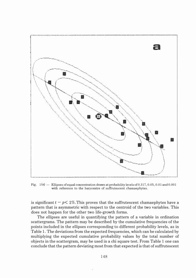
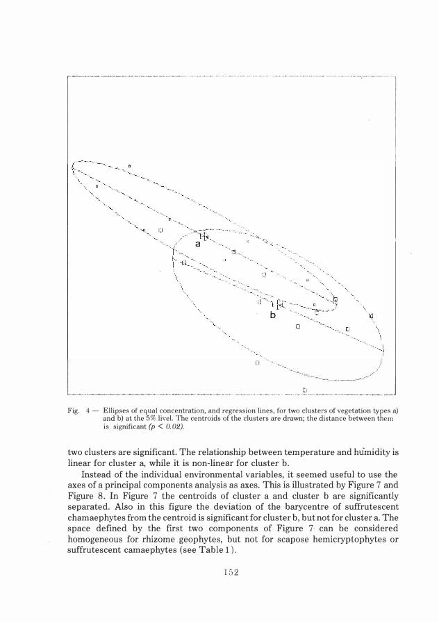
Cl '----------·--------- .............. ,. ...•..•...... • . -··· ............................ ____ _ _j Fig. 4 - Ellipses of equa! concentration, and regression lines, for two clusters of vegetation types a)

and b) at the 5% livel. The centroids of the clusters are drawn; the distance between them is significant (p < O. 02).

two clusters are significant. The relationship between temperature and hùmidity is linear for cluster a, while it is non·linear for cluster b.

Instead of the individua! environmental variables, it seemed useful to use the axes of a principal components analysis as axes. This is illustrated by Figure 7 and Figure 8. In Figure 7 the centroids of cluster a and cluster b are significantly separated. Al.so in this figure the deviation of the barycentre of suffrutescent chamaephytes from the centroid is significant for cluster b, but not for cluster a. The space defined by the first two components of Figure 7 can be considered homogeneous for rhizome geophytes, but not for scapose hemicryptophytes or suffrutescent camaephytes (see Table 1).

152

r···· - ·-·· -···· - . ···-·-. -----

-.�,,

· ..

.,,""-...

i�

---.. a

"·=:::· -<�···� ..

.... _,_

a

Fig. 5 - Ellipses of equa! concentration around the barycentre B of suffrutescent chamaephytes of cluster b), and its centroid C, with reference to temperature and pH. The distance between the barycentre and centroid is significant (p < 0.04).

153

-------- ,, ., w-,,,.,-........... , ..... . .. , --- ........ _ ............................................................... -............ ----�

Fig. 6 - Ellipses of equa! concentration at the 5% leve! around the centroids (C) and barycentres (B) of suffrutescent chamaephytes of clusters a) and b). The variables are humidity and temperature. The distances are significant between the barycentres of clusters a) and b), the centroids of cluster a) and b), the centroid of cluster a) and the barycentre of cluster b) and the centroid and barycentre of cluster b). The slopes of the regression lines are significantly different, while the intercepts are not.

In respect of the three life-growth forms, one can conclude that, in the space defined by the environmental variables and the 20 vegetation types, their niches (sensu Hutchinson, see Hurlbert, 1981) are shifting in an orderly fashion as one passes from the relatively, driest and most basic soils to the most humid and acid soils according to the sequence: suffrutescent chamaephytes, scapose hemi­cryptophytes and rhizome geophytes (Figure 8). In this sequence the barycentre of suffrutescent chamaephytes is significantly distant from the barycentres of the other two life .. growth forms. The sequence corresponds also with decreasing

154

·--

a

a

\·�---... _ .... •*" ...

a ··--.... ________ , ... ------·

'-------------------�------...,...---,--.... ,. ..... - ... ....... .. ----.. --

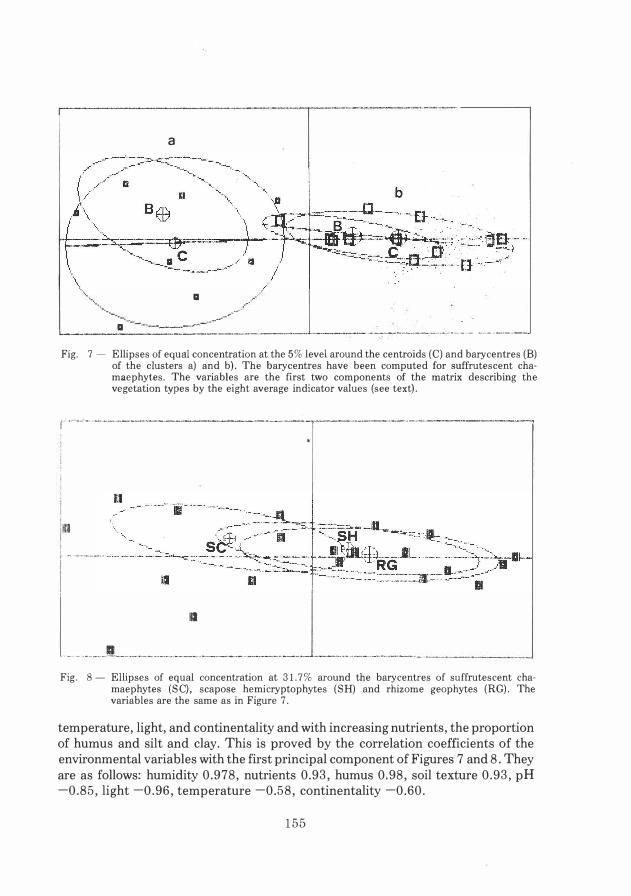
Fig. 7 - Ellipses of equa! concentration at the 5% leve! around the centroids (C) and barycentres (B) of the clusters a) and b). The barycentres have been computed for suffrutescent cha­maephytes. The variables are the first two components of the matrix describing the vegetation types by the eight average indicator values (see text).

r····-------------------r----------------�

lii

...................... 111 __ . ., ______________ .,__ _______ _

Fig. 8 - Ellipses of equa! concentration at 31.7% around the barycentres of suffrutescent cha­maephytes (SC), scapose hemicryptophytes (SH) and rhizome geophytes (RG). The variables are the same as in Figure 7.

temperature, light, and continentality and with increasing nutrients, the proportion of humus and silt and clay. This is proved by the correlation coefficients of the environmental variables with the first principal component of Figures 7 and 8. They

are as follows: humidity 0.978, nutrients 0.93, humus 0.98, soil texture 0.93, pH -0.85, light -0.96, temperature -0.58, continentality -0.60.

155

AJrnowledgements. The work has been supported by a CNR grant for the project "Structure and Dynamics of forests". We are grateful to prof. D.W. Goodall for reading and correcting the text.

References

Cliff A.D. and Ord J.K. (1981) - Spatial process. Models and applications. Pion, London.

Da.boni L. (1967) - Calcolo delle probabilità. Boringhieri, Torino.

Feoli E. and Ganis P. (1986) -Autocorrelation for measuring predictiuity in community ecology: An example with structural and chorological data {rom mixed forest types of NE ltaly. Coenoses 1: 53-56.

Hurlbert S.H. (1981)-A gentle depilation of the niche:Dicean resource sets in resource hyperspace. ln May, R.M. (ed.) Evolutionary theory, 5: 177-184. The University of Chicago, Chicago.

Lagonegro M. e Feoli E. (1985) - Analisi multiuariata di dati. Manuale d'uso di programmi Basic per persona! computers. Libreria Goliardica, Trieste.

Landolt E. (1977) - Oekologische Zeigerwerte zur Schweizer Flora. Ber. Geobot. lnst. ETH, 64: 64-207.

Mardia K.V., Kent J.T. and Bibby J.M. (1979) - Multiuariate analysis. Academic Press, London, New York.

Orloci L. (1973) - Ranking characters by a dispersion criterion. Nature 244: 371-373.

Pol<lini L. (1982) - Ostrya carpinifolia-rich woods and bushes of Friuli-Venezia Giulia. Studia Geobotanica 2: 69-122.

Zar J.H. (197 4) - Biostatistical Analysis. Prentice-Hall. Englewood Cliff, N.J.

Authors' address: Prof. Dr. E. Feoli Prof. Dr. M. Lagonegro Dipartimento di Biologia, Università degli Studi di Trieste, 34100 Italia

156

Appendix.

The data for the program must be prepared in a sequential file in which the information is contained in blocks of records, each block containing in order: 1) the alphanumerical code for the variable for which the analysis is required (type wanted);

2) the score for the variable (prod);3) the scores of the variables which, two by two, define the space (variables); these may be severa! and

their number is placed after the "prod" variable. The following is an example of the data structure as printed:

(type wanted, prod, variables) casu 20 casu 10 casu 9

2.5 0.9 0.7

2.7 1.3 1.3

9.8 6.9 5.3

10.75 9.88 6.97

In this case there are 3 objects described by variable casu (type wanted), the scores of casu for the three objects, and the four variables which, two by two, define the spaces. The file must be typed as follows for both the BASIC and the FORTRAN versions:

casu 20 2.5 2.7 9.8 10.75 casu 10 0.9 1.3 6.9 9.88 casu 9 0.7 1.3 5.3 6.97

The listings of the program are given helow, both in BASIC and FORTRAN.

28 ijMibli°m� fLLIPLOT II (H.Lagonegro-1985) 30 ON ERROR GOTO 2010 40 IHPUT'give n.lines,n.ellipses n.vars in data table '·NL NTY HV 50 DIH TIPOi(HU, PROD (HU I VAR5(HltHV) /E5UHU lll (!OO)!HtY> 1 $LO (HTY) /51 (HTY) 1 E53 (HTY> ,E55(HTY), ELV (NTY)60 DIH X (HL, HTY) iv (HL, NTY 1 , R (HL, H V) 1-,1,G (HTY) , Yt. (NTV) , !�5 (NTV 1 , IK52 (HM, UN (HTY 1 , 52 (NTY), E52 (HTV) 70 !NPUT'�ive fi ena1e for data • ;DAti 80 OPEN"i , Nl, DAH 90 FOR !=1 TO HL 100 INPUTN1 A TIPOi (!) 110 INPUT Ml, rROD (!) 120 FOR J=1 TO HV 130 INPUTNl, VARS <I, J > 140 NEXT J 150 NEXT I 160 CLOSEN1 170 INPUT'print data-vin '; 5Hi 180 IF SNi= 'n' THEN 170 190 LPRINT' --- data table ---• 200 FOR !=1 TO HL 210 LPRINT TIPOi (!) ; PROD (I) ; 220 FOR J=l TO NV 230 LPRINT VARSU,,J>;

157

240 HEXT J 250 LPRINT 260 HEXT I 270 INPUT'give labels of couple of wanted vars-to stop give 0,0 • ;H,H 280 K=l 290 IF H•H=O THEH END 300 INPUT'tyee wanted/no '; TV$ 310 IF TV$= no' THEH 270 320 IHPUT'weighting-unif/prod ';TI$ 330 PETOT=O 340 HU=O 350 FOR I=l TO HL 360 A$=TIPO$ m 370 IF A$0 TV$ THEH 440 380 HU=HU+l 390 PESI<NUl=PROD(Il 400 X (HU, Kl =VARS (l, Hl 410 V<HU,Kl=VARS(l,H) 420 R(HU K)=I 430 PETOt=PETOT +PROD (l) 440 HEXT I 450 UH(K)=HU 460 XG(K) =O 470 VG(Kl=O 480 FOR I=l TO HU 490 PESI (l) =PESI m /PETOT 500 IF Tl$='unif' THEH PESI(l)=l/HU 510 XG (Kl =XG (K) +X(!, K) •PESI (l) 520 VG(K)=VG(K)+V(I,K)IPESI(l) 530 HEXT I 540 SX2=0 550 SV2=0 560 SXV=O 570 FOR I=l TO HU 580 PES2=PESI (I) 590 SX2=SX2+PES2•(X<I,Kl-XG(K))'2 600 SV2=SV2+PES2• (V(!, K)-VG(K)) '2 610 SXV=SXV+PES2* (X(!, Kl-XG(K)) * (V(I, KHG(K)) 620 HEXT I 630 SX=SQR (5X2) 640 SV=SQR (5V2) 650 52(K)=(SX2+SV2)/2 660 RO=SXV / (SX•SV) 670 IF SH$='y' THEH LPRINT' Ellipse n. =';K 680 IF SH$='.y' THEN LPRIHT'sx=';SX;' sy=';SV;' ro=';RO 690 INPUT'g1ve residua! % • ;REP 700 IF SH$='y' THEH LPRINT'residual X=' ;REP 710 REP=-LOG (REP /100) 720 IF ROl , 99999 THEH RO=, 99999 730 IF RO (-, 99999 THEN RO=-, 99999740 Xl=XG(KHQR(REP)ISX 750 X2=XG(Kl+SQR(REP)•SX 760 DX= (X2-Xl) /99 770 IKSl (K) =Xl 780 IK52(K)=X2 790 FOR I=l TO 100 800 ELI(l,1,K)=DX•(I-l)+Xl 810 XS=(EL!(l�l,Kl-XG(K))/SX820 B=-2•RO•b 830 C=X5'2+REP* (R0'2-1) 840 BC=ABS (BA2-41C) 850 VSl=,51(-B-SQR<BC)) 860 V52=. 5* (-B+SQR <BC)) 870 Ell(I,2,K)=VSl•SV+VG(K) 880 EU (!Ì3, K) =VS2•SV+VG (K) 890 NEXT 900 IF SH$='n' THEH 1090 910 LPRIHT 'aode is '; TU 920 LPRIHT':< is ';N'-th var. and � is ';H;"-th' 930 LPRINT'x froa '.;Xl;' to 'iPi, y froa 'i,Ell(l,2,K) ;' to ';Ell(l00,2,K) 940 LPRINT' centro1d has X=';�G(�);' V=';VG(�) 950 LPRINT' points have 960 FOR I=l TO NU 970 LPRINT R(l,K);' x=';X(l,Kl;' y=';V(l,K);' weight=';PESI(l)

158

980 HEXT I 990 HSCB=O:FOR 1=1 TO HU-1:IF X<I

\K)(=X(I+1

ÌK) THEH 1040

1000 ACI=X<I K) :X<I,K)=X(l+1,Kl:X !+1,K)=AC 1010 ACI=V<(Kl :V(l,K)=V<I+1,K) :V(I+1,K)=ACI 1020 ACI=R(I,K) :R(l,K)=R(I+1,Kl :R(l+1,K)=ACI 1030 NSCB=1 1040 HEXT I 1050 lF HSCB O O THEN 990 1060 LPRIHT'horizontal sequence' 1070 FOR !=1 TO HU:LPRINT R(I,K);1080 HEXT I: LPRIHT 1090 K=K+1:IF K<=NTV THEN 300 1100 INPUT'plot-scale factors diff/equal ';OIEQ$1110 CLS:SCREEN 3 1120 HX=-1E+30 1130 HV=HX 1140 HHX=1E+30mo HHV=HNX 1160 FOR K=1 TO HTV1170 HU=UH(K) 1180 FOR !=1 TO NU

m� �� ��il x��1:b1���N

H��X=

X(M\)

1210 IF HV ( V<I �l THEN HV= V<I, K1 1220 IF HNVl V (Ì, K) THEN HNV= Y (I, K)1230 NEXT I NEXT K 1240 FOR K=l TO NTY 1250 FOR !=1 TO 100 1260 IF ELI<I,1,K)(HNX THEN HNX=ELI(I,11K) 1270 lF ELl(l,1,KllHX THEN HX=EL!(l,l,K1 1280 lF EL! (I, 2, K) <HNV THEN HNV=ELI (I, 2 /l1290 IF EL!(! 2 K) lHV THEN HV=ELI (I 2 K1 1300 IF EL!([:3:K)(HNV THEN HNV=Eutr:3,K)1310 IF ELin,,31

,K)lHV THEN HV=ELI<I,3,Ki 1320 NEXT I: NE.._T K 1330 LPRIHT'x froa '·HNX·' to '·HX·' y fro1 '·HNV·' to '·HV 1340 FX=400/ (HX-HHX)' ' ' ' ' ' ' mo FV=320/(HV-HHVl: lF OIEQ$='di ff' THEH 1380 1360 IF FX < =FV THEH FV=FX 1370 lF FV<=FX THEH FX=FV 1380 LINE (O, 49)-(420 399), B 1390 LPRINT'scale factors: h=• ;FX;' fy=' ;FV 1400 XO=-HNX•FX + 5 1410 V0=399+HNV•FV-5 1420 LIHE (X0,49HX0,399)1430 LIHE <O,VOH420,VO) 1440 FOR K=l TO NTV 1450 NU=UH(K) 1460 XX=(XG(K)-HHXl•FX+5 1470 VV=399-(VG ( Kl-HHVl*FV-5 1480 AR=K+4:UR=,83•AR:CIRCLE<XX VV) AR 1490 LINE (XX-AR

iVVHXX+AR, VV) \INt (XX, VV-URHXX, VV+UR)

1500 FOR !=1 TO 00 1510 EL! (I, 1, K)=(ELI (I, 1, Kl-HHXl*FX+5 1520 EL! (I ,2, K)=399-(Ell (l ,2, Kl-HNVl•FV-5 mo EU (l ,3, K)=399-(ELI (I, 3, Kl-HNV) •FV-5 1540 NEXT I mo UNE (ELl(1

11òK) ,ELI(l,2,K))-(Ell(l,1,K) ,Ell(l,3,K))

1560 FOR !=2 TO O mo Xl=ELI(l-1,1/l 1580 X2=ELI (I, 1, K1 1590 Vl=ELI (I-1, 2, K)1600 V2=ELI (I, 2, K) 1610 V3=ELI(I-1,3/l1620 V4=ELI (I 3 K1 1630 LINE m;viHX2,V2) 1640 LIHE (Xl,V3HX2,V4) 1650 HEXT I 1660 UNE (EL! (100, 1, K), EL! (100 ,2, K) HELI (100, 1, Kl, EU (100, 3, Kll 1670 FOR I=l TO NU 1680 XX=(X(l Kl-HNXl•FX+5 1690 VV=399-(V(! Kl-HNV> •FV-5 1700 UNE (XX-K,YV-KHXX+K,VV+Kl .,B

159

1710 NEXT I 1720 51=0 :52=0: 53=0: 54=0: 55=0 1730 FOR !=1 TO HU:51=51+X(l�K)A2:52=52+X(l�K) :53=53+X(l1,K>•Y(l,K) 54=54tY(l,K) :55=55tY(!,K)A2:HEXT I 1740 PENO= (NU•S3-52•54) / (NU•�1-S2A2) : THOT= b4-52•PEKO) /Nu 1750 X=! K51 (K) : Y=PENO•X+TNOT: XX= (X-HNXl *FX+5: YY=399-(Y-HNY) •FY-5: X= I K52 ( K) : Y=PEHO*X+ TNOT 1760 XXX=(X-HNX>*FX+5:YYY=399-(Y-HNY)*FY-5:L!HE <XX, YYHXXX YYY) 1770 IF SN$='y' THEN LPRIHT'regression line: ';PENO/*:< '/HR$(44-5GH(TNOT» ;ABS<TNOT> 1780 SLO (K) =PENO: E51 (K) =51: ES2 (K) =52: E53 (K) =53: E55 (�) =55: tLV (K) =THOT: NEXT K 1790 LOCATE , 55: IHPIJT'plot on printer-y/n ';HAH$ 1800 IF HAH$='y' THEH LCOPY O 1810 IF NTY=1 THEN 1980 1820 LPRINT:LPRINT' *** C011parison a1ong centroids1,slopes & intercepts ***':LPRINT 1830 FOR K=1 TO NTY-1:FOR J=K+1 TO NTY:H=UN(K) :H=UN(J) 1840 5T2= «N-1) *52 (K) t (H-1) *52 (Jl) / (H+N-2) 1850 O=SQR( (XG(K)-XG (J) )A2t <YG<K>-YG (J) )A2): TI=O*SllfHH*H/ (5T2*(H+N))) 1860 T = TI : OF =H+H-4: GOSUB 2030 1870 LPRlNT'�air '·K·' and '·J·' --- t='·TI·' deg,of freedo1='·0F·" prob(7.)='·A 1880 RE551=E55 (K)-lES3 (K) A2) ÌES1 (K): RE552=ES5(JHES3(J)A2) /ES! (Jj 1890 E52XY= (RE551 +RE552) / (N+H-4) : 581B2=SQR (E52XY /E51 (K) +E52XY /E51 (J)) 1900 TI=ABS <SLO (K)-5LO (J)) /SB1B2: T=TI OF=H+N-4: GOSUB 2030 1910 LPRINT' slopes t' =';TI·• d, freedoa=' · OF · • with prob m=• · A 1920 BlC!=(E53(Kl+E53(J)) / <ES! (K) +E51 (J)) :HEi=ES2(K) /N: HE2=E52<Jj /H :OlHE=HE1-HE2 1930 BOH=DIHEA2/ (E51 (K) +E51 (J)) : TI= <ELV <1 )-ELV <2>-B!Cl * <OIHE)) /SQR (E52XY* ( 1/N+ 1/H+BOH)) . TI =ABS (TI) 1940 OF =H+N-3: T = TI : GOSUB 2030 1950 LPRlNT' intcpts t"='·TI·' d.freedol=';OF;' with prob(Z)=';A 1970 HEXT J: LPRlNT: NEXT K ' ' 1980 CLS 1990 GOTO 270 2000 EHO 2010 PRlNT'kapel1eister n, ';ERR;' line n, • ;ERL 2020 END 2030 REH-Subroutine Probt 2040 T=ATN<T/SQR(OF)) IF OF=1 TliEN A=,5-T/3,14159 2050 lF OF=2 THEN A=,5*(1-SlH(T)) 2060 IF DF=3 THEN A=,5-(1/3,14159>•<T+COS<T>*SIN(T)) 2070 IF OF <4 THEN GOTO 2180 2080 lF OF/2)1NT(OF/2) THEN 2140 2090 C=l : Q=2 2100 U=1 : FOR 1=2 TO Q STEP 2 : U=U*<l-1)/l 2110 HEXT l : C=C+U*(ABS<COS(T)))AQ 2120 Q=Q+2 : IF Q(OF THEN 2100 2130 A=,5•<1-(5!N<T>>•C> : GOTO 2180 2140 C=1 : Q=2 2150 U=l : f'OR 1=2 TO Q STEP 2 : U=Ull/(!+1) : NEXT l 2160 C=C+U*<AB5(C05(T)))AQ : Q=Q+2 : IF Q<OF-1 THEN 2150 2170 A=, 5-(1/3, 14159)•<T+C05<T>*SIN<n*C> 2180 A=A*200 2190 RETURN

160

$LARGE PROGRAl1 ELLIOIS

C---ORAWS EQUI-COHCEHTRATIOH ELLIPSES FOR OBJECTS OESCRIBEO C---BV PAIRS OF VARIABLES-COl1f'ARES THEH REGRESSIOH LIHES C---WRITTEH BV H.LAGONEGR0-1986 <FROH BASIC VERSION)

COIIHOH SLO (25) 1,ELV (25) , ES! (25) f ES2 (25) l53 (25), E55 (25) , HL, HTV

I HIJ PR00(200) vAR5(200,25) ,PES (200) ELl(l00,3 25) 2X (2ÒO, 25), V(2Ò0125) � IR(200,25), XG(25j, VG (25), EtSt (25)3 EK52 (25) KUN (2,) 5�2 (25) CHARACTER' •4TIP0(200) ,AOO, TIOO, SHOO, TISO ,OIEQS CHARACTER •IOOAFOO WR!TE(l,1)' GIVE H.LIHES,H.ELLIPSES,H.VARIABLES' REAO O •) HL NTV NV WRITE(•/l' 'GIVÉ FILENAHE OF DATA'REAO(t, (AIO)' )OAFOO OPEN(! /ILE=OAFOO, STATUS=' OLO') 00 lOltO !=! Hl REAO(I,' (AA)1)T!PO(!)

REAO (!A•) PftOO (l)00 lO!tO J=l,NV

10120 REAO(lit)VARS(!,J)

CLOSE ( ) WRITE(111)' PRINT DATA-VIN'REAO(t (A4)')5NOO IF (SNOO, EQ,' N' ) GOTO 10260

\IRITE(• 1)' --- DATA TAilE ---' 00 10200 I=! Hl

10200 WRITE(l,t)T!POm ,PROO(l), (VARS(l,J) ,J=l,NV) 1 FORIIAHlX A4 Gll.4, (IX lOGl0,3)) 10260 WR!TE(I, * j' tIVE INOEXES OF WANTEO VARS-TO STOP GIVE O, O'

REAO(t, t)N,H K=I

lF (H, EQ, O) STOP 10290 WR!TE(111)' TVPE WANTEO/N'

REAO(t (A4)' )Tl00 IFn!ÒO.EQ,'N')GOTO 10260

1/RITE(I 11)' WEIGHTIHG-UHIF /PROO'REAO(tÒ (A4)')TISO PETOT= NU=O 00 10430 1=1,NL AOO= TIPO m lF(AOO.NE.TIOO)GOTO 10430

NU=NU+l PESUNU) =PROO m

X (NU, K) =VARS (!, N)V (NU 1, K) =VARS (1, H) !R(Nu,K)=l PETOT=PETOT +PROO m

10430 CONTINUE KUN(K)=NU XG(K)=O VG(Kl=O 00 10510 1=1,NU PESI (l) =PESI (I) /PETOT IF mso, EQ,' UNIF' l PESI m =1./FLOAHHU) XG(K)=XG(K)+X (1, K) •PESI m

10510 VG(K)=VG(K)+V(l,Kl•PESI(l) SX2=0 SV2=0 SXV=O 00 10600 1=1,NU PES2=PESim SX2=SX2+PES2•(X(l, Kl-XG(K) )112 SV2=SV2+PES2t(V(l K)-VG(K))112

10600 SXV=SXV+PES2•(X (!: K)-XG(K) )t(V(l, K)-VG(K)) SX=SQRT (5X2) SV=SQRT (SV2) 552 (K) = (5X2+SV2) /2 RO=SXV / (SX•SVl IF(SND-0.EQ.'V')IIR!TE(t,1)' ELLIPSE H.=' K IF(SNOO.EQ.'V')WR!TE(t I)' SX=' SX ' SV=1 SV ' RO=' RO WRITE (I, I)' GIVE RESIOUAU%)' ' ' ' ' '

161

READ(* ilREP lF(SNDÒ.EQ,'V' lWRITE(*,*l' RESIDUAL ¼=' ,REP REP=-LOG <REP /100! IF <RO, GT, <, 99999) l RO=, 99999 lF(RO.LT, (-.99999)) R0=-,99999 Xl =XG ( Kl -SQRT (REPl •SX X2=XG ( Kl +SQRT (REPl •SX DX= (X2-Xll /99, EKSl (Kl=Xl EKS2 (Kl=X2 DO 10870 1=1,100 Ell(l 1 Kl=OX•<Hl+Xl XS= <Ei'..l tr, 1, KHG <Kl l /SX B=-2, •RO•XS C=XSH2+REP* (ROH2-1.) BC=ABS (8H2-4, IC) VSl =, 5* (-B-SQRT (BCl l VS2=, 5* <-B+SQRT <BC) l ELI (l, 2, Kl=VSl•SV+VG(Kl

10870 ELl (l � 3, Kl =VS2•SV+VG (KllF<SNuO.EQ, 'N' )GOTO 11180 WRITE (I 2) mo

2 FORHAT(1 HOOE 15:' ,A4l WRITE<* 3lN H

3 FORHAT<1 X ÌS ',14 '-TH VAR. V 15 ',14,'-TH'l WRITE<*14lX1 X2,fLÌ(1,2,p ElfUD0,2,p , , , 4 FORHAT< X FROH: ,Gll.4, fo: ,Gll.4, V FROH: ,Gll.4, TO: ,

1G11.4l WRITE<* 5)XG(Kl VG(Kl

5 FORHAT<1 CENTROÌD HAS X=' 1G11.4,' V=' ,G11,4l WRITE <*Ò*l' POlNTS HAVE DO 1096 1=1 NU

10960 WRITE<* 6llR\r,Kl X<I Kl V<I Kl ,PESI(l) 6 FORHAT<1 POS, IN TAB, = 1 14 ' X=' G11, 4 ' V=' Gll, 4 ' WElGHT='

1, Gll , 4 l ' ' ' ' ' ' 10980 NSCB=O

00 11110 I=l,NU-1 IF<X<I

ÌKl .LE.X<I+l,KllGOTO 11110

ACI=X( ,Kl X<I,Kl=X<I+l,Kl X(l+l,Kl=ACI ACI=V<l Kl V<I,Kl=V(l+l,K) V<I +l!Kl =ACI IACI= R(l KlIR(l, Kl=lR(I+l, K) IR(l+l, Kl=IACI NSCB=l

11110 CONTINUE IF<NSCB.NE.OlGOTO 10980 WRITE (161)' HORIZOHTAL SEQUENCE'00 1115 1=1 HU

11150 WRITE<•{7)IR!r!Kl 7 FORHAT< X,2014 •

11180 K=K+l IF (K.LE, HTV) GOTO 10290 WRITE(*,*l' GlVE PLOT-SCALE FACTOR:DIFF/EQUA'REAO<•, <A4l' lOlEQS RHX=-1,E+30 RHV=RHX RHHX=1.E+30 RHNV=RHNX 00 11350 K=l, NTV NU=KUN(Kl DO 11340 I =1 NU IF(RHX.LT.X<Ì Kll RHX= X(! Kl IF<RHNX,GT.X(Ì1,Kll RHHX= Xh1Kl IF<RHV.LT.V<I tll RHV= V<I,K1 IF <RHNV, GT. V (Ì, Kl l RHNV= V<I, Kl

11340 CONTINUE 11350 CONTINUE

00 11450 K=l,NTV DO 11440 I=l.100

162

IF (Ell (I, 1, Kl , LT, RHHX)RHHX=ELI (I, 1, K) IF (Ell <I 1 K) , GT. RHX> RHX=ELI <I 1 K) IF(Ell <( 2: K) ,LT .RHHV)RHNV=ELI l(21 K) IF(Ell<I 2 KLGT.RHV)RHV=Ell<I 2 K1 IF<ELI <(3: K) .LT .RHNV>RHNV=ELI l(31 K) IF (Ell (I, 3, K) , GT, RHVl RHV=ELI <I, 3, Ki

11440 CONTINUE 11450 CONTINUE

WRITEO19)RHNX,�HX{RHNV1RHY_ , , , 9 FORHAT< X FROH ,G 1.4, TO ,G11.4, -- V FROH ,G11.4, TO' 1 Gl1,4) FX=100/ <RHX-RHHX) FV=100/ (RHV-RHNV) IF(DIEQS.EQ.'DIFF')GOTO 11520 IF<FUE.FV> FV=FX IF <FV, LE, FXl FX=FV

11520 CALL PLONPA (RHHX,RHX4RHHV, RHV, FX, FV, SNDO)

IF<NTV,EQ,1)GOTO 126 O WRITE (161) '0 I COHPARISON FOR CENTROIDS, SLOPES, INTERCEPTS'DO 1263 K=l NTV-1 DO 12610 J=K+1,NTV N=KUH(K) H=KUN(J) ST2= (FLOAT (H-1) 1552 (K) +FLOAT (H-1) 1552 (J)) /FLOAT (H+N-2) D=SQRT ( (XG(KHG (J) l H2+ (VG(KHG (J) )H2) TI=0ISQRT <FLOAT (HIN)/(ST21FLOAT (H+N))) T=TI 0F=H+H-4 CALL PROB T<T, DF A) WRITE<f110)K J1h Df,A , , _, , _, 10 FORHAT< PAIR ,14, & ,14, -- T- ,G11.4, 0.FR.- F6.0,

1' HO PROB. (%)=' G11.4) RE551=E55(KHE53(K)H2) /E51 (K) RES52=E55(JHE53(J)H2)/E51 (J) ES2XV= (RESS1 +RE552) /FLOAT (H+H-4) SB1B2=5QRT (ES2XV /E51 (K) +E52XV /E51 (J)) TI=ABS (SLO <K>-SLO(J)) /58182 T=TI 0F=H+H-4 CALL PROBT<TtDF �Al WRITE(1 11)T ,0t A

11 FORHAT<1 SLOP(S T=' ,G11.4,' D.FR,=' ,F6,0,' HO PROB. <U=' 1 G11.4) élCI= (E53 (K) +E53(J)) / <ES1 (K) +E51 (J)) AHE1=E52 (K) /FLOAT<H) AHE2=E52 (J)/FLOAT<H) DIHE=AHE1-AHE2 BOH=0IHEH2/(E51 (K)+E51 (J)) TI=<ELV(1HLV(2HICl1<DIHE)) /SQRT (E52XV1<1./FLOAT (H) +

11, /FLOAT (H) +BOH>) TI=ABS(TI) DF=H+N-3 T=TI CALL PROBT <Tt0F �Al WRITE (1 12lT Dt A

12 FORHAT<1 ÌNTCPTS T=' ,G11.4,' 0.FR.=' ,F6.0,' HO PROB. <U=' 1 G11,4)

12610 CONTINUE WRITE(1 •l'

12630 CONTINU( 12640 CONTINUE

GOTO 10260 END SUBROUTINE PROBT<T, 0F, Al T=ATAH<T /SQRT<DF> l IF <DF .EQ, 1.) A=, 5-T /3 .14159

IF<DF.EQ.2.l A=,5•(1.-SIH<nl IF <DF, EQ, 3,) A= , 5-(1.13 .14159) • <T +COS (T) •SIN m) IF<DF.LT,4,) GOTO 12970 !F((OF/2,) .GT:INT<DF/2,))GOTO 12870 C=t. Q-2 12780 U=l,'

163

IQU=Qt, 5 00 12800 1=2, IQU,2

12800 U=U•FLOAHI-1)/FLOAHilC=C+U• (ABS (COS ml l **Q

Q=Q+2' IF (Q, LT, OFl GOTO 12780

A=, 5• (1.-(SIH ml •ClGOTO 12970

12870 C=l, Q=2,

12890 U=l. IQU=Qt, 5

12910 ��u!�mTlrf Jj��Ai(l+ll C=C+U• <ABS ( COS (T) l l HQ Q=Qt2, IF(Q,LT.(OF-1,llGOTO 12890

A=, 5-(1,/3, 14159l* <T+COS(Tl*SIN(T) •Cl 12970 A=A•200,

RETURH EHO SUBROUTINE PLOHPA(RHNX,RHX,RHNV RHV FX,FV SNDOlCOHIION SLO (25l lLV (25l, E51 (25l

fÉ52 <25l , ES3 (25l , E55 (25l , Hl, HTV

1,HV PR00(200l vAR5(200,25l,PES (200l EL!(l00,3 25l 2X(200

l25l, rnÒÒ�25l �IR(200,25l ,XG<25l, VG(25l ,EK51 <25l

31,EK52 25l ,KUN<2,l 1,5)2(25l

i.:HARACTER PLOT<lDt, 102! CHARACTER •45HOO 00 100 1=1 102 00 100 J=l' 102

100 PLOHI,Jl=éHAR(32l00 101 !=1 102 PLOT<l Il=éHAR(45l PLOT<1621 ll=CHAR(45lPLOHI li =CHAR (33l

101 PLOT(I: 102l =CHAR (33l WR!TE(* llFX FV FORHAT<1 SCALE FACTORS - FX=' ,Gll.4,' FV=' ,G11.4l X0=-RHIO)FX t 1, V0=102,+RNNV•FV-1,CALL LIHE (XO, 1., XO 1,102,, PLOT, 33l CALL UNE (1., VO, 10t,, VO, PLOT, 45l00 12220 K=l, NTV NU=KUH(Kl 00 11710 !=1 100 EL! (I, 1, Kl =<ÉLI (! 1 Kl-RHHXl•FX+l. EL!(! 2 Kl=102,-<ÉLÌ(I 2 Kl-RHHVl•FV-1.

11710 ELl((3:Kl=102, -(EL! n :3: Kl-RHHVl•FV-1. 00 11820 !=1,100X2=ELI (I, 1, K1 V2=ELI (I, 2, Kl V4=ELI (! i 3, KlIX2=X2+,, IV2=V2+, 5IV4=V4+, 5 PLOHIV2, IX2l =CHAR (42l

11820 PL0l(IV4, IX2l =CHAR (42l 51=0, 52=0,53=0, 54=0,55=0, 00 12000 1=1,NU51=51+X(I Kl**2 52=52+ X<I ' K l 53=53+X<l:Kl*V(l,Kl54=54+V<I, Kl

12000 55=55+V<I Kl **2 PENO= <FLOAT (NUl •53-52•54l / <FLOAT (NUl •S1-52H2l THOT= (54-52•PENOl /FLOAT (NUl AX=EK51 <Kl AV=PEHO•AX t THO T XX=CAX-RHHXl•FX+l,

164

VV=102, -<AV-RHNV) •FV-1, AX=EKS2<Kl AV=PENO•AX+ TNOT XXX=<AX-RHNXl•FX+l, VVV=102, -<AV-RHNVl •FV-1, CALL LINE(XX VV,XXX VVV,PLOT 43) lF<SNOO.EQ.'V'l IIRltE<*,*l' REGRESSION LINE:' \IRITE<•, 2lPENO, TNOT

2 FORHAH' SLOPE=' ,G11.4,' lNTERCEPT=' ,G11.4l SLO (Kl =PENO ES1 (Kl=Sl E52(Kl=S2 ES3(Kl=53 E55(Kl=55 ELV<Kl=TNOT 00 11880 1=1 NU XX=<X<I, Kl-RHNX>•FX+l.

VV=102, -(V<l, Kl-RHNVl •FV-1. lXX=XX+, 5 lVV=VV+, 5

11880 PLOT<IVV I lXXl =CHAR (64+KlXX=<XG(K1-RHNXl•FX+1. VV=102, -(VG (Kl-RHNVl•FV-1.

lXX=XX+, 5 lVV=VV+, 5 PLOT<IVV, lXXl =CHAR (35)

12220 CONTINUE \IRITE<•, 1)' PLOT ON PRINTER-V=l/N=O' READ<•,•>HAH lF <HAH, EQ, Ol RETURN DO 3 1=1 102

3 IIRITE<•i4l <PLOT<I,Jl ,J=l, 102)

4 FORHAH X,102A1l RETURN END SUBROUTINE UNE <Xl, VI A X2, V2, PLOT, NCl CHARACTER PLOT<102, 10ll OX=X2-X1 OV=V2-V1 lF <DX, EQ, O, l DX=!, E-9 A=OV/OX B=V1-A•X1 PA=OX/100 DO 5 l=l,101 XX=Xl+<I-ll•PA VV=A•XX+B IF (XI.EQ, X2lVV= l lF (V!.EQ, V2lXX=l lXX=XX+, 5 lVV=VV+, 5 lF<IXX.GT, 102.0R, lXX,LT, !) lXX=I IF<IVV ,GT, 102.0R. lVV .LT, Il lVV=I

� PlOHIVV, IXX)•CHAR<MC! RETURN ENO

165