Hands-on tutorial to Genome-wide Association Studies (GWAS)Ümit Seren

Exploring Plant Variation Data Workshop

Jul. 1st-3rd 2015

trans-National Infrastructure for Plant Genomic Science

https://goo.gl/bSX3De

Outline• Introduction

• Motivation

• Why plants (A. thaliana)?

• Population Structure

• GWAS methods

• Linear model

• Non-parametric test

• Linear Mixed Model

• Advanced Linear Mixed Models

• Caveats & Problems

• Hands-on tutorial

• Introduction to GWA-Portal

• Step by step guide

• Summary

Suggested literature

• Hastie, Tibshirani, and Friedman. (2009) The Elements of

Statistical Learning: Data Mining, Inference, and Prediction. A

very good book. A pdf can be downloaded here: http://www-

stat.stanford.edu/~tibs/ElemStatLearn/.

• Lynch and Walsh. (1998) Genetics and Analysis of

Quantitative Traits. This book is an outstanding classical

reference for quantitative geneticists.

• Nature Genetics. (2008-2013) Genome-wide association

studies. Series about best practices for doing GWAS in

humans. http://www.nature.com/nrg/series/gwas/index.html

IntroductionMotivation, Why plants (A. thaliana) ?, Population Structure

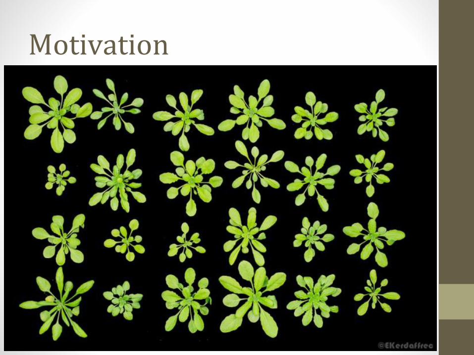
Motivation

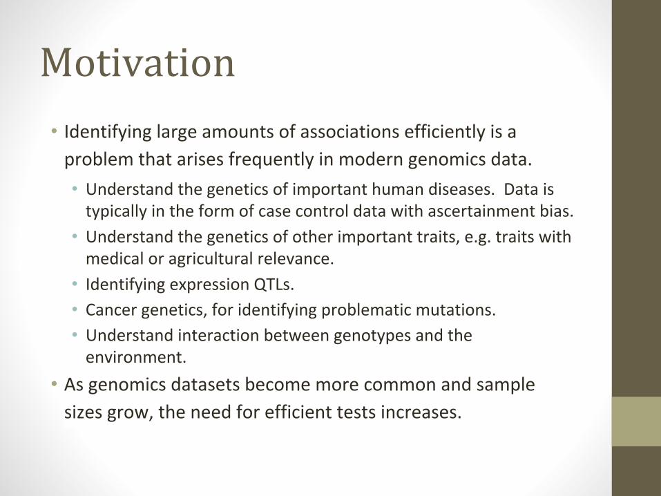
Motivation

• Identifying large amounts of associations efficiently is a

problem that arises frequently in modern genomics data.

• Understand the genetics of important human diseases. Data is typically in the form of case control data with ascertainment bias.

• Understand the genetics of other important traits, e.g. traits with medical or agricultural relevance.

• Identifying expression QTLs.

• Cancer genetics, for identifying problematic mutations.

• Understand interaction between genotypes and the environment.

• As genomics datasets become more common and sample

sizes grow, the need for efficient tests increases.

Motivation

• Studying the genetics of natural variation

• Understanding the genetic architecture of

traits of ecological and agricultural

importance

• Identifying the genomic regions that control

genetic variation

• Test association at many variants instead of some and hypothesis-free instead of hypothesis-driven.

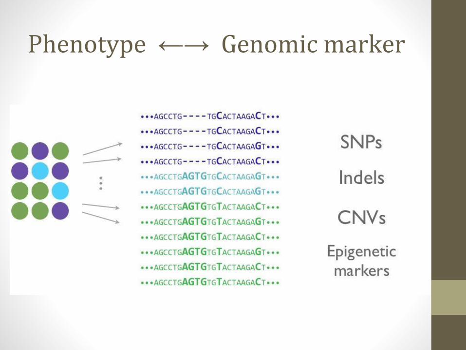
Phenotype ←→ Genomic marker

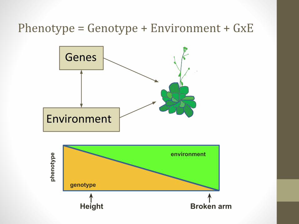
phen

otyp

e

genotype

environment

Height Broken arm

Phenotype = Genotype + Environment + GxE

Genes

Environment

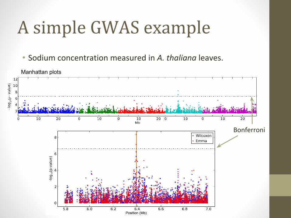
A simple GWAS example

• Sodium concentration measured in A. thaliana leaves.

Bonferroni

Manhattan plots

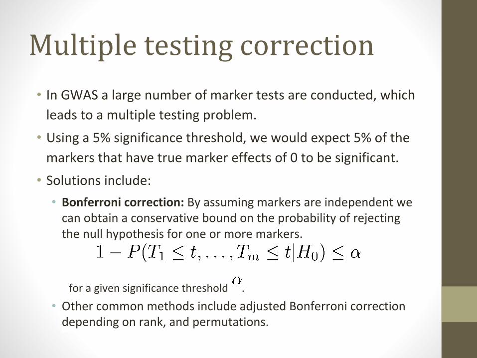
Multiple testing correction

• In GWAS a large number of marker tests are conducted, which

leads to a multiple testing problem.

• Using a 5% significance threshold, we would expect 5% of the

markers that have true marker effects of 0 to be significant.

• Solutions include:

• Bonferroni correction: By assuming markers are independent we can obtain a conservative bound on the probability of rejecting the null hypothesis for one or more markers.

for a given significance threshold .

• Other common methods include adjusted Bonferroni correction depending on rank, and permutations.

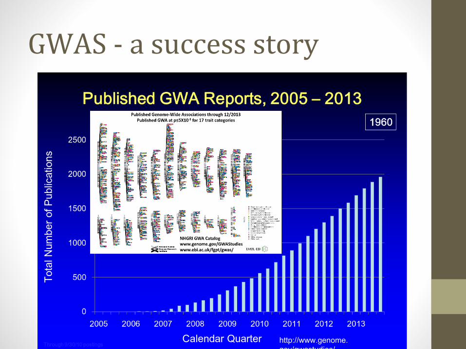
GWAS - a success story

http://www.genome.gov/gwastudies/

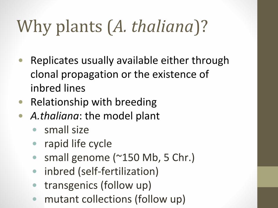
Why plants (A. thaliana)?

• Replicates usually available either through clonal propagation or the existence of inbred lines

• Relationship with breeding• A.thaliana: the model plant

• small size• rapid life cycle• small genome (~150 Mb, 5 Chr.)• inbred (self-fertilization)• transgenics (follow up)• mutant collections (follow up)

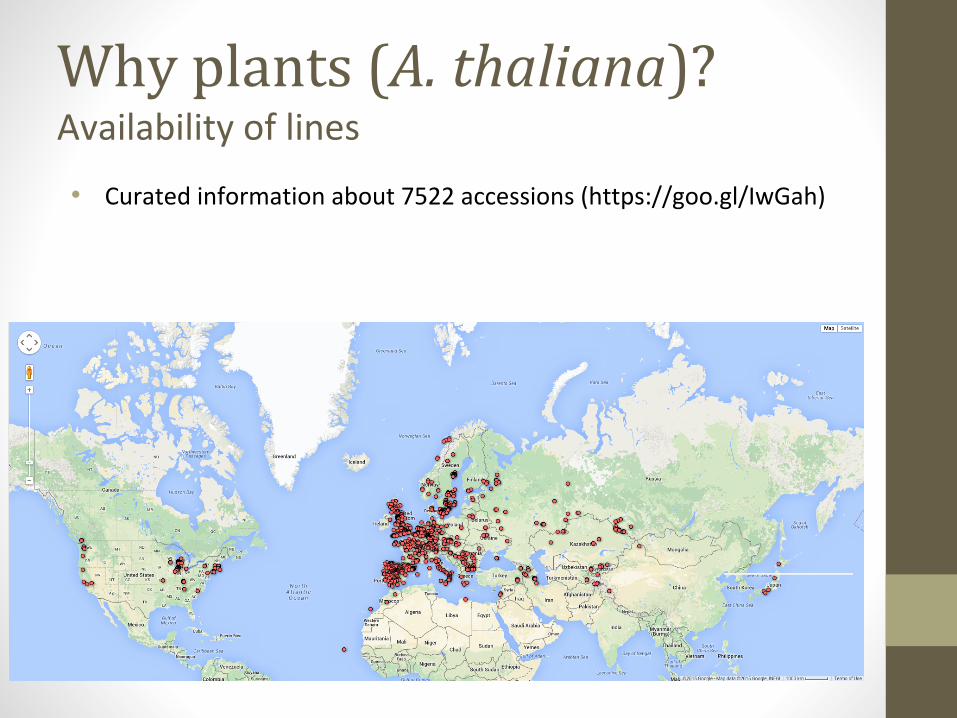
Why plants (A. thaliana)?Availability of lines

• Curated information about 7522 accessions (https://goo.gl/IwGah)

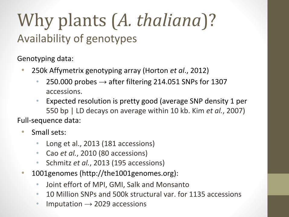
Why plants (A. thaliana)?Availability of genotypes

Genotyping data:

• 250k Affymetrix genotyping array (Horton et al., 2012)

• 250.000 probes → after filtering 214.051 SNPs for 1307 accessions.

• Expected resolution is pretty good (average SNP density 1 per 550 bp | LD decays on average within 10 kb. Kim et al., 2007)

Full-sequence data:

• Small sets:

• Long et al., 2013 (181 accessions)• Cao et al., 2010 (80 accessions)• Schmitz et al., 2013 (195 accessions)

• 1001genomes (http://the1001genomes.org):

• Joint effort of MPI, GMI, Salk and Monsanto• 10 Million SNPs and 500k structural var. for 1135 accessions• Imputation → 2029 accessions

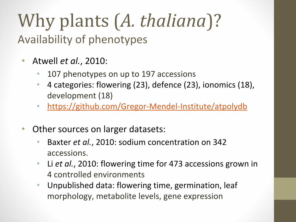
Why plants (A. thaliana)?Availability of phenotypes

• Atwell et al., 2010:• 107 phenotypes on up to 197 accessions• 4 categories: flowering (23), defence (23), ionomics (18),

development (18)• https://github.com/Gregor-Mendel-Institute/atpolydb

• Other sources on larger datasets:• Baxter et al., 2010: sodium concentration on 342

accessions.• Li et al., 2010: flowering time for 473 accessions grown in

4 controlled environments• Unpublished data: flowering time, germination, leaf

morphology, metabolite levels, gene expression

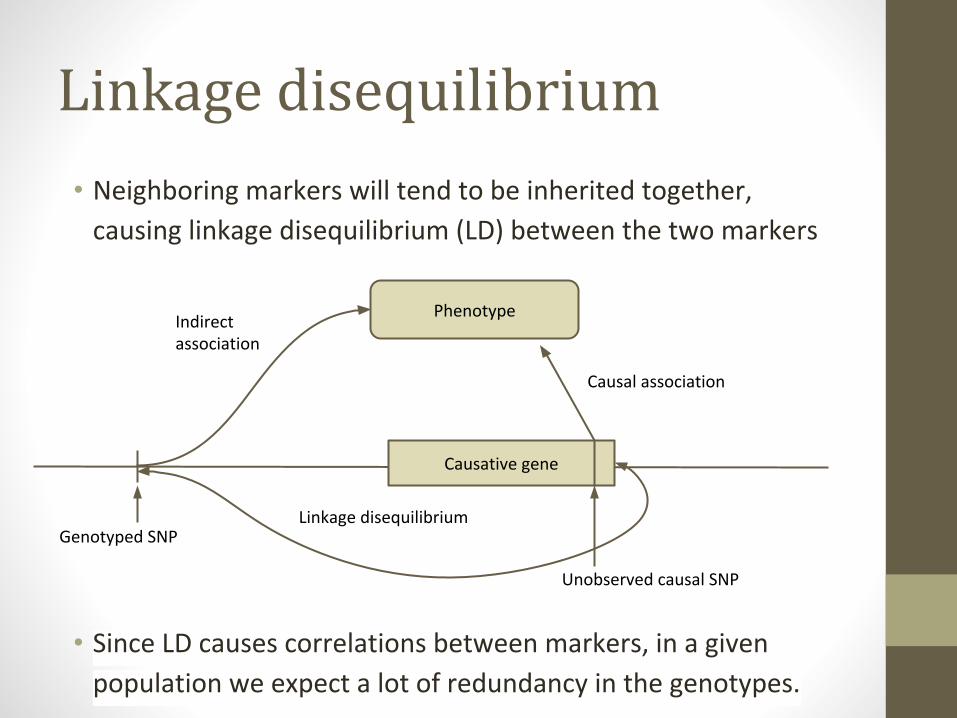
Linkage disequilibrium

• Neighboring markers will tend to be inherited together,

causing linkage disequilibrium (LD) between the two markers

• Since LD causes correlations between markers, in a given

population we expect a lot of redundancy in the genotypes.

Causative gene

Phenotype

Genotyped SNP

Indirect association

Causal association

Linkage disequilibrium

Unobserved causal SNP

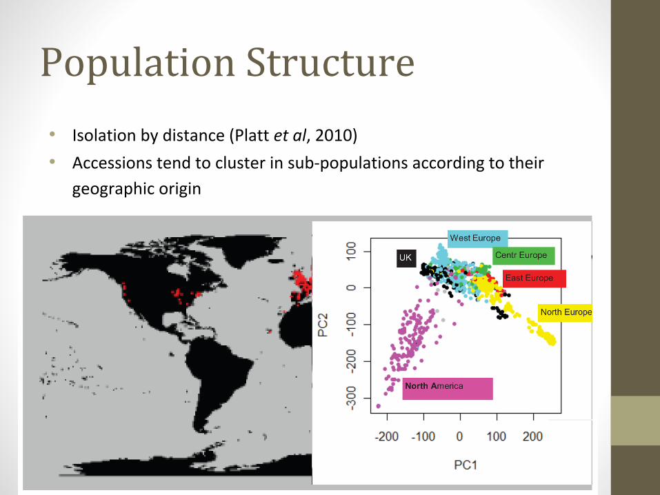
Population Structure

• Isolation by distance (Platt et al, 2010)

• Accessions tend to cluster in sub-populations according to their

geographic origin

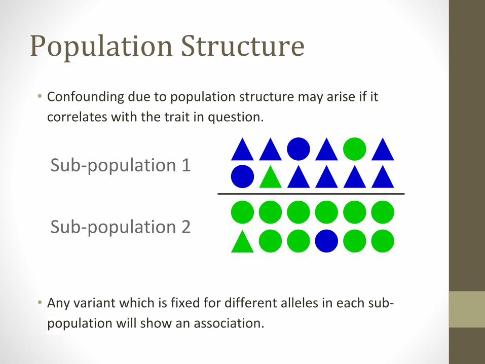
Population Structure

• Confounding due to population structure may arise if it

correlates with the trait in question.

• Any variant which is fixed for different alleles in each sub-

population will show an association.

Sub-population 1

Sub-population 2

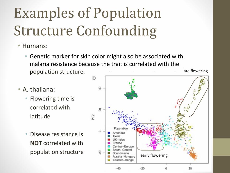
Examples of Population Structure Confounding

• Humans:

• Genetic marker for skin color might also be associated with malaria resistance because the trait is correlated with the population structure.

• A. thaliana:• Flowering time is

correlated with

latitude

• Disease resistance is

NOT correlated with

population structure

late flowering

early flowering

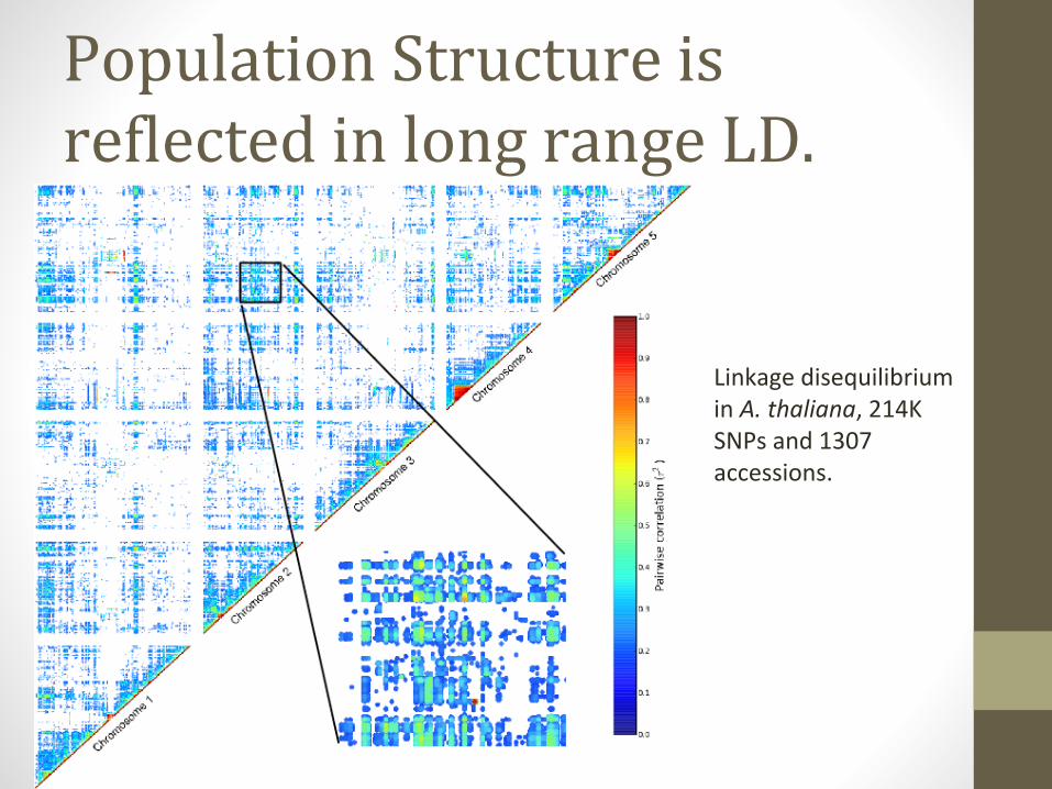
Population Structure is reflected in long range LD.

Linkage disequilibrium in A. thaliana, 214K SNPs and 1307 accessions.

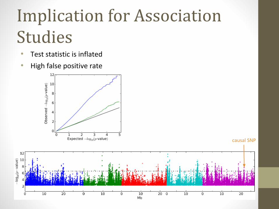
Implication for Association Studies• Test statistic is inflated

• High false positive rate

causal SNP

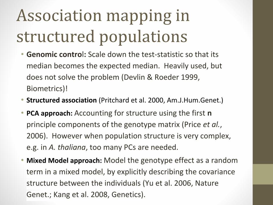
Association mapping in structured populations

• Genomic control: Scale down the test-statistic so that its

median becomes the expected median. Heavily used, but

does not solve the problem (Devlin & Roeder 1999,

Biometrics)!

• Structured association (Pritchard et al. 2000, Am.J.Hum.Genet.)

• PCA approach: Accounting for structure using the first n

principle components of the genotype matrix (Price et al.,

2006). However when population structure is very complex,

e.g. in A. thaliana, too many PCs are needed.

• Mixed Model approach: Model the genotype effect as a random

term in a mixed model, by explicitly describing the covariance

structure between the individuals (Yu et al. 2006, Nature

Genet.; Kang et al. 2008, Genetics).

GWAS Methods

Linear Model, Non-parametric test, Linear Mixed Model, Advanced Linear Mixed Models & Caveats & Problems

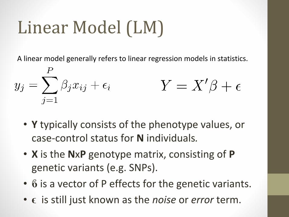
Linear Model (LM)

A linear model generally refers to linear regression models in statistics.

• Y typically consists of the phenotype values, or case-control status for N individuals.

• X is the NxP genotype matrix, consisting of P genetic variants (e.g. SNPs).

• ϐ is a vector of P effects for the genetic variants.

• ϵ is still just known as the noise or error term.

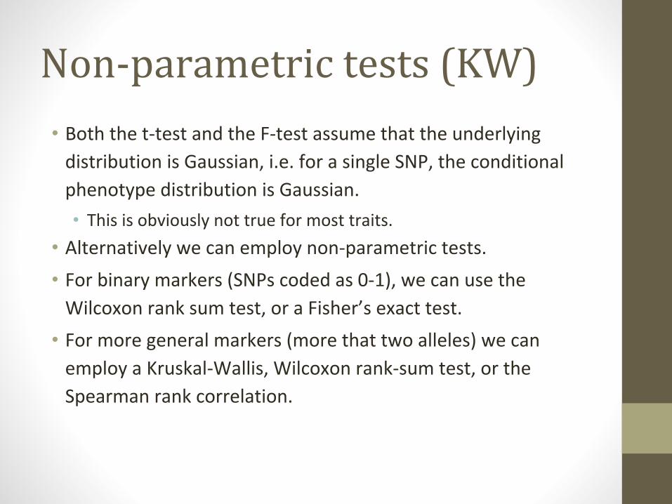
Non-parametric tests (KW)

• Both the t-test and the F-test assume that the underlying

distribution is Gaussian, i.e. for a single SNP, the conditional

phenotype distribution is Gaussian.

• This is obviously not true for most traits.

• Alternatively we can employ non-parametric tests.

• For binary markers (SNPs coded as 0-1), we can use the

Wilcoxon rank sum test, or a Fisher’s exact test.

• For more general markers (more that two alleles) we can

employ a Kruskal-Wallis, Wilcoxon rank-sum test, or the

Spearman rank correlation.

Linear Mixed Model (LMM)

• Linear model and Non-parametric tests don’t account for

population structure

• Initially proposed in Association mapping by Yu et al. (2006)

• Y typically consists of the phenotype values, or case-control status

for N individuals.

• X is the NxP genotype matrix, consisting of P genetic variants (e.g.

SNPs).

• u is the random effect of the mixed model with var(u) = σ g K

• K is the N x N kinship matrix inferred from genotypes

• ϐ is a vector of P effects for the genetic variants.

• ϵ is a N x N matrix of residual effects with var(ε) = σ e I

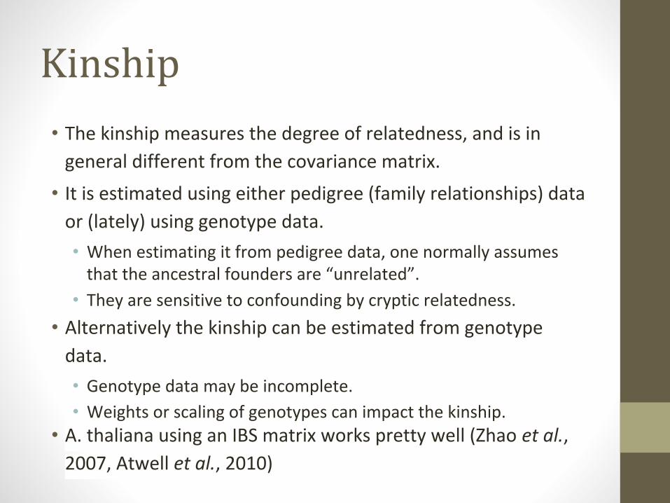
Kinship

• The kinship measures the degree of relatedness, and is in

general different from the covariance matrix.

• It is estimated using either pedigree (family relationships) data

or (lately) using genotype data.

• When estimating it from pedigree data, one normally assumes that the ancestral founders are “unrelated”.

• They are sensitive to confounding by cryptic relatedness.

• Alternatively the kinship can be estimated from genotype

data.

• Genotype data may be incomplete.

• Weights or scaling of genotypes can impact the kinship.• A. thaliana using an IBS matrix works pretty well (Zhao et al.,

2007, Atwell et al., 2010)

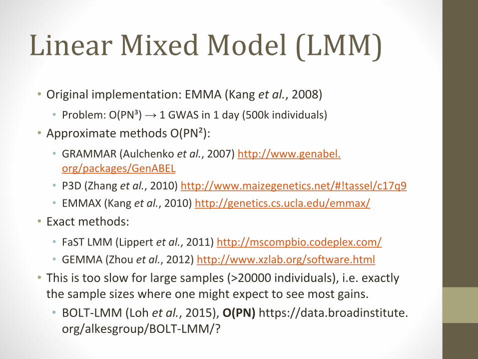
Linear Mixed Model (LMM)

• Original implementation: EMMA (Kang et al., 2008)

• Problem: O(PN³) → 1 GWAS in 1 day (500k individuals)

• Approximate methods O(PN²):

• GRAMMAR (Aulchenko et al., 2007) http://www.genabel.org/packages/GenABEL

• P3D (Zhang et al., 2010) http://www.maizegenetics.net/#!tassel/c17q9

• EMMAX (Kang et al., 2010) http://genetics.cs.ucla.edu/emmax/

• Exact methods:

• FaST LMM (Lippert et al., 2011) http://mscompbio.codeplex.com/

• GEMMA (Zhou et al., 2012) http://www.xzlab.org/software.html

• This is too slow for large samples (>20000 individuals), i.e. exactly the sample sizes where one might expect to see most gains.

• BOLT-LMM (Loh et al., 2015), O(PN) https://data.broadinstitute.org/alkesgroup/BOLT-LMM/?

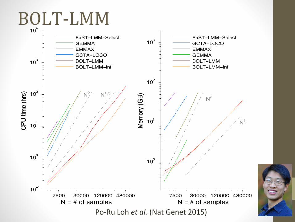
BOLT-LMM

Po-Ru Loh et al. (Nat Genet 2015)

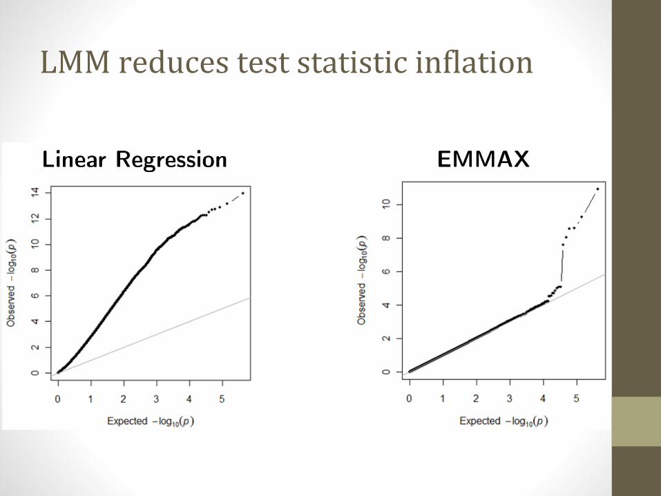
LMM reduces test statistic inflation

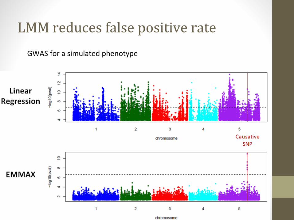
GWAS for a simulated phenotype

LMM reduces false positive rate

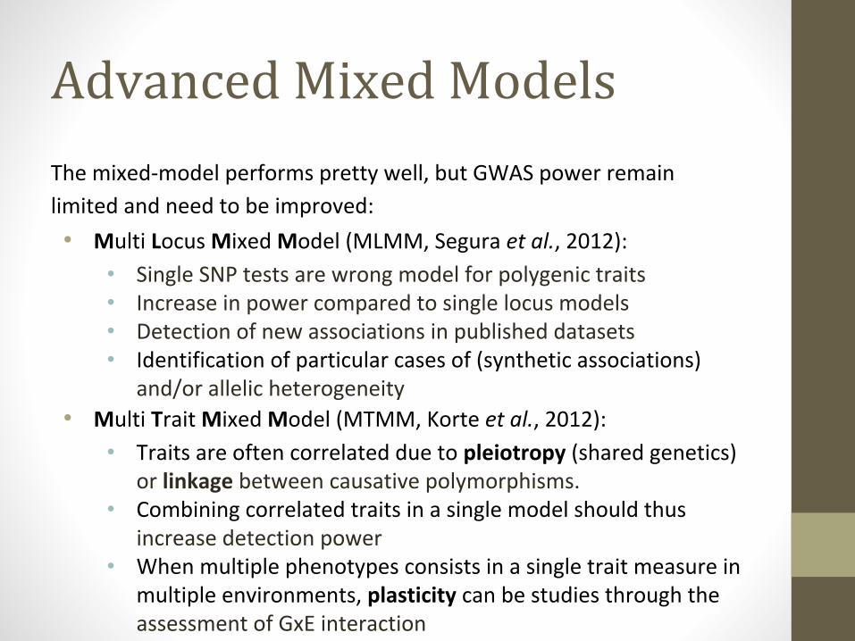
Advanced Mixed Models

The mixed-model performs pretty well, but GWAS power remain

limited and need to be improved:

• Multi Locus Mixed Model (MLMM, Segura et al., 2012):

• Single SNP tests are wrong model for polygenic traits• Increase in power compared to single locus models• Detection of new associations in published datasets• Identification of particular cases of (synthetic associations)

and/or allelic heterogeneity• Multi Trait Mixed Model (MTMM, Korte et al., 2012):

• Traits are often correlated due to pleiotropy (shared genetics) or linkage between causative polymorphisms.

• Combining correlated traits in a single model should thus increase detection power

• When multiple phenotypes consists in a single trait measure in multiple environments, plasticity can be studies through the assessment of GxE interaction

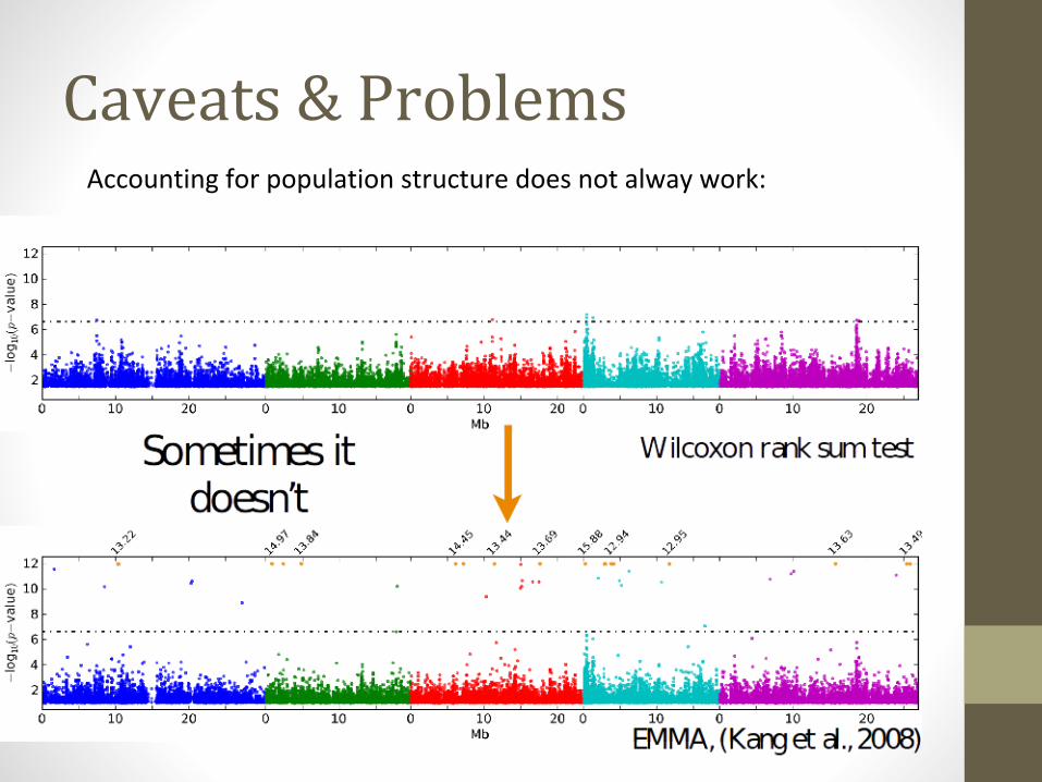
Caveats & ProblemsAccounting for population structure does not alway work:

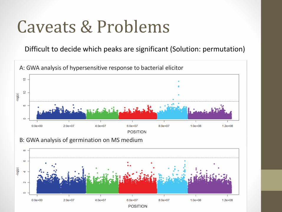
Caveats & ProblemsDifficult to decide which peaks are significant (Solution: permutation)

Caveats & ProblemsPeaks are complex and make it difficult to pinpoint causative site

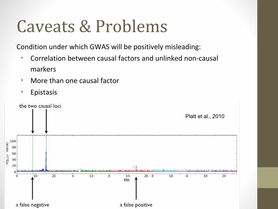
Caveats & ProblemsCondition under which GWAS will be positively misleading:

• Correlation between causal factors and unlinked non-causal

markers

• More than one causal factor

• Epistasis

Platt et al., 2010

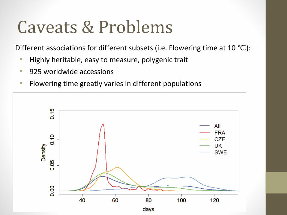
Caveats & ProblemsDifferent associations for different subsets (i.e. Flowering time at 10 °C):Different associations for different subsets (i.e. Flowering time at 10 °C

• Highly heritable, easy to measure, polygenic trait

• 925 worldwide accessions

• Flowering time greatly varies in different populations

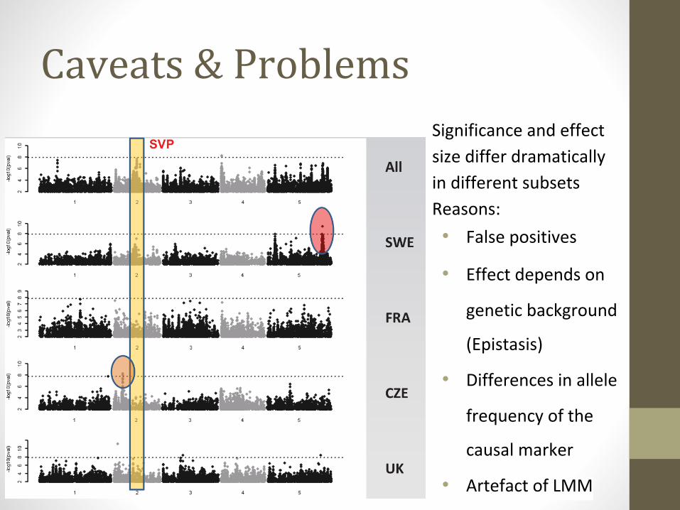
Caveats & ProblemsSignificance and effect

size differ dramatically

in different subsets

Reasons:

• False positives

• Effect depends on

genetic background

(Epistasis)

• Differences in allele

frequency of the

causal marker

• Artefact of LMM

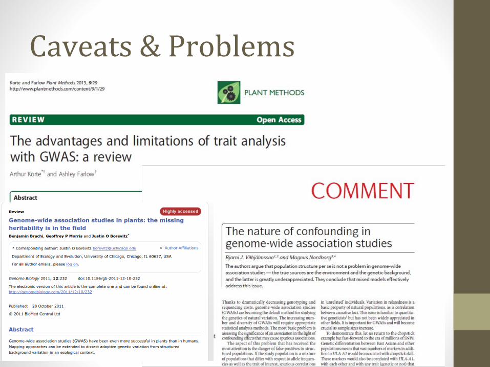
Caveats & Problems

Hands-on tutorial

Introduction to GWA-Portal, Step-by-step guide and Resources

Introduction to GWA-Portal

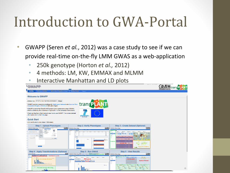
• GWAPP (Seren et al., 2012) was a case study to see if we can

provide real-time on-the-fly LMM GWAS as a web-application

• 250k genotype (Horton et al., 2012)• 4 methods: LM, KW, EMMAX and MLMM• Interactive Manhattan and LD plots

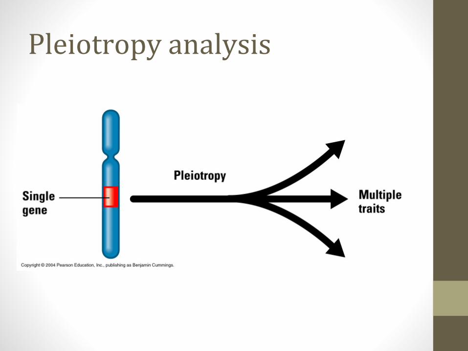
Pleiotropy analysis

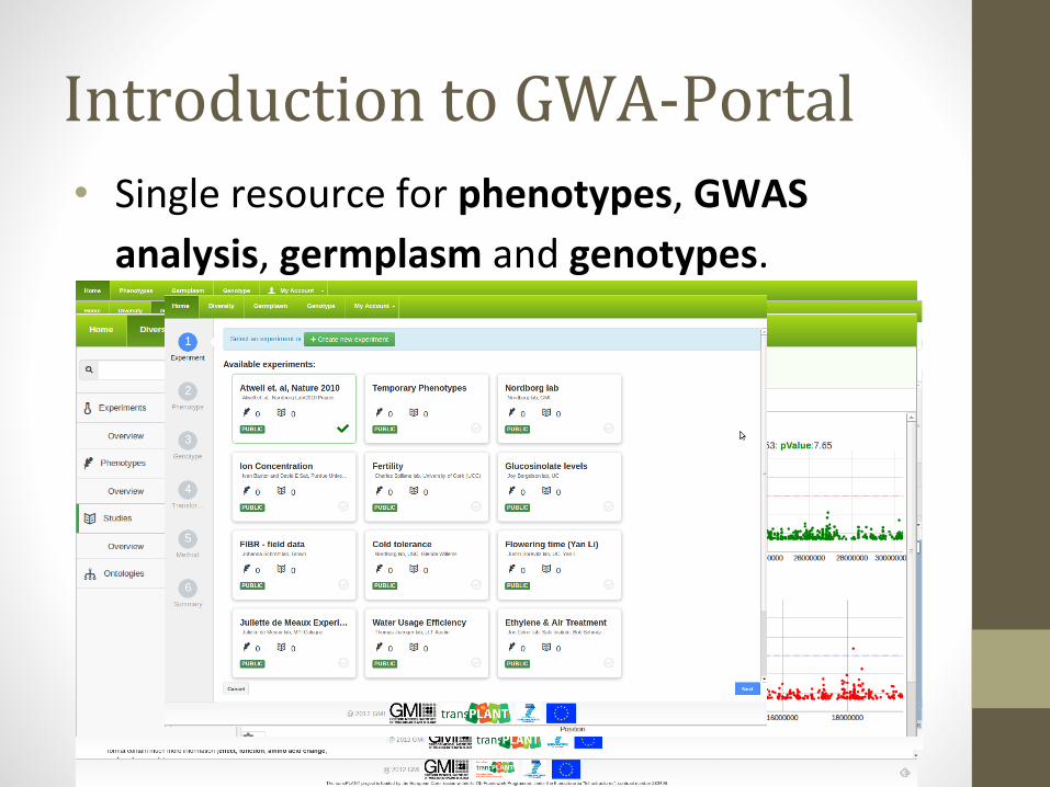
Introduction to GWA-Portal• Single resource for phenotypes, GWAS

analysis, germplasm and genotypes.

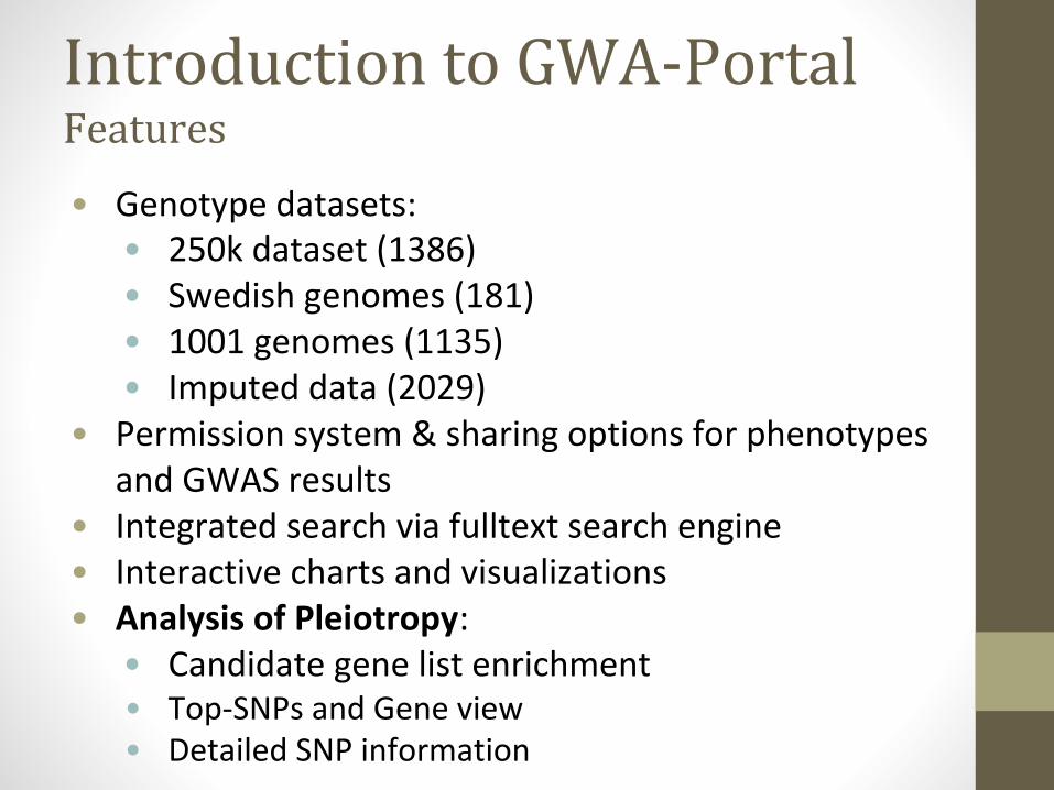
Introduction to GWA-PortalFeatures

• Genotype datasets:• 250k dataset (1386)• Swedish genomes (181)• 1001 genomes (1135)• Imputed data (2029)

• Permission system & sharing options for phenotypes and GWAS results

• Integrated search via fulltext search engine• Interactive charts and visualizations• Analysis of Pleiotropy:

• Candidate gene list enrichment• Top-SNPs and Gene view• Detailed SNP information

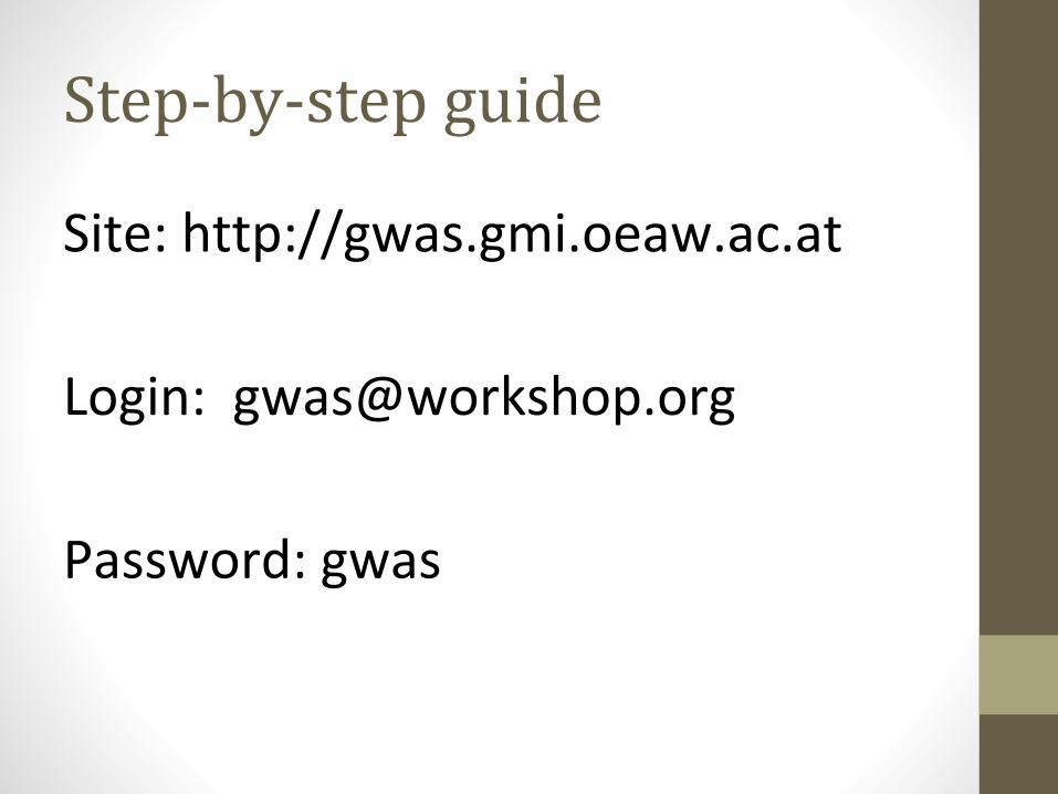
Step-by-step guide

1. Groups of 2 - 3 users

2. Download phenotype file

3. Each groups creates a study

4. Upload the phenotype and create a GWAS analysis

5. 5-10 minute coffee break (until GWAS analysis is

finished)

6. Interactive discovery using Manhattan plots (filtering,

zooming, etc)

7. Display detailed SNP information

8. View candidate gene list enrichment analysis

9. Meta-analysis of pleiotropy

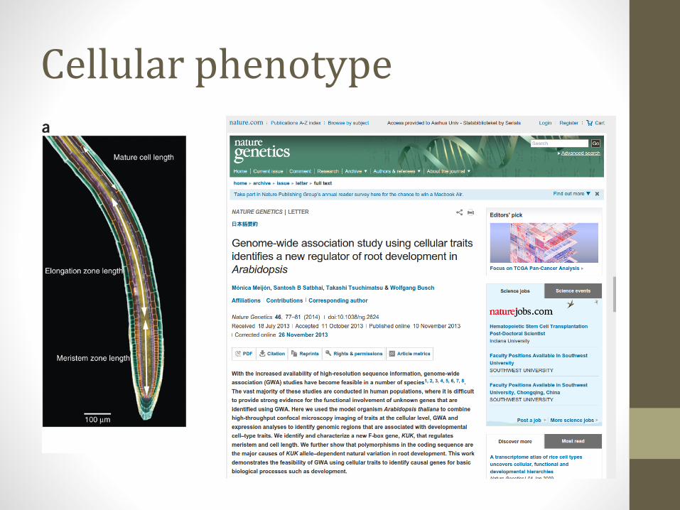
Cellular phenotype

•

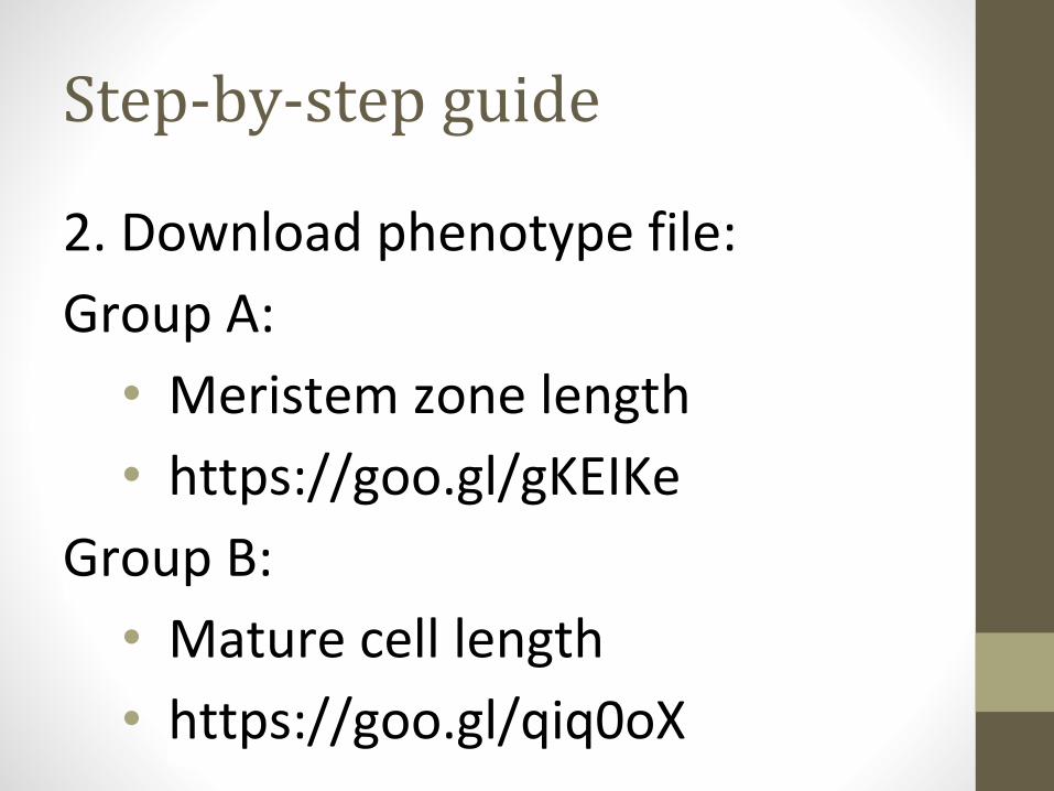
Step-by-step guide

2. Download phenotype file:

Group A:

• Meristem zone length

• https://goo.gl/gKEIKe

Group B:

• Mature cell length

• https://goo.gl/qiq0oX

Step-by-step guide

Site: http://gwas.gmi.oeaw.ac.at

Login: gwas@workshop.org

Password: gwas

SummaryWhat did we learn?, Resources & Acknowledgements?

Summary

• GWAS is a powerful tool to understand the genetics of natural

variation.

• Methods are fast enough to do GWAS on big sample sizes in

reasonable time

• Population structure confounding can cause issues

• Linear Mixed Model can help address this issue• BUT GWAS is not without challenges to be aware of

• Epistatic interaction• Allelic heterogeneity• GWAS on sub-samples • …

• Web-based tools like GWA-Portal allow to mine the GWAS data,

look at the information from different perspectives and uncover

previously unknown pleiotropic effects.

Summary

THE END

Acknowledgements

GMI:

• Radka Slovak

• Arthur Korte

• Magnus Nordborg

• Nordborg lab

BiRC:

• Bjarni Vilhjálmsson

BSC:

• Josep Lluis Gelpi

• Laia Codo

The transPLANT project is funded by the European Commission within its 7th Framework Programme

under the thematic area "Infrastructures", contract number 283496.

Resources

• GWAPP (Seren et al.):

• URL: http://gwapp.gmi.oeaw.ac.at• Code: http://github.com/timeu/GWAPP

• GWA-Portal:

• URL: http://gwas.gmi.oeaw.ac.at• Code: https://github.com/timeu/GWA-Portal

• Phenotypes:

• Meijón et al., 2013 (Nature Genetics)• http://www.nature.com/ng/journal/v46/n1/full/ng.2824.html

• PyGWAS:

• https://pypi.python.org/pypi/PyGWAS/0.1.4• https://registry.hub.docker.com/u/timeu/pygwas/

References

• Estimating kinship

• Weir, BS, Anderson, AD, & Hepler, AB. (2006) Genetic relatedness analysis: modern data and new challenges. Nat Rev Genet.

• Kang, H, Zaitlen, N, et al. (2008). Efficient control of population structure in model organism association mapping. Genetics.

• Kang, H. M., Sul, J. H., Service, S. K., et al. (2010) Variance component model to account for sample structure in genome-wide association studies. Nat Genet.

• Powell, JE, Visscher, PM, & Goddard, ME. (2010) Reconciling the analysis of IBD and IBS in complex trait studies. Nat Rev Genet.

References

• Estimating heritability

• Visscher, P. M., Hill, W. G., & Wray, N. R. (2008) Heritability in the genomics era - concepts and misconceptions. Nat Rev Genet.

• Yang, J., Benyamin,B, et al. (2010) Common SNPs explain a large proportion of the heritability for human height. Nat Genet.

• Yang, J., et al. (2011) Genome partitioning of genetic variation for complex traits using common SNPs. Nat Genet.

• Deary, I. J., et al. (2012). Genetic contributions to stability and change in intelligence from childhood to old age. Nature.

• Korte, A., Vilhjálmsson, B. J., Segura, V., et al. (2012) A mixed-model approach for genome-wide association studies of correlated traits in structured populations. Nat Genet.

• Zaitlen, N., & Kraft, P. (2012) Heritability in the genome-wide association era. Hum Genet.

References

• Controlling for population structure in GWAS using mixed

models.

• Yu, J., Pressoir, G., Briggs, W. H., Vroh Bi, I., Yamasaki, M., et al. (2006) A unified mixed-model method for association mapping that accounts for multiple levels of relatedness. Nat Genet.

• Zhao, K, et al. (2007). An Arabidopsis example of association mapping in structured samples. PLoS Genet.

• Kang, HM, et al. (2008) Efficient control of population structure in model organism association mapping. Genetics.

• Zhang, Z, Ersoz, E, et al. (2010) Mixed linear model approach adapted for genome-wide association studies. Nat Genet.

• Kang, H. M., et al. (2010) Variance component model to account for sample structure in genome-wide association studies. Nat Genet.

References

• Controlling for population structure in GWAS using mixed models.• Lippert, C., Listgarten, J., et al. (2011) FaST linear mixed models

for genome-wide association studies. Nat Meth.• Segura, V., Vilhjálmsson, B. J., et al. (2012) An efficient multi-

locus mixed-model approach for genome-wide association studies in structured populations. Nat Genet.

• Listgarten, J., Lippert, C., et al. (2012) Improved linear mixed models for genome-wide association studies. Nat Meth.

• Pirinen, M, et al. (http://arxiv.org/abs/1207.4886) Efficient computation with a linear mixed model on large-scale data sets with applications to genetic studies. Submitted to the Annals of Applied Statistics.

• Zhou, X., & Stephens, M. (2012). Genome-wide efficient mixed-model analysis for association studies. Nat Genet.

References

• Principal components

• Price, A. L., Patterson, N. J., et al. (2006) Principal components analysis corrects for stratification in genome-wide association studies. Nat Genet.

• Patterson, N., Price, A. L., & Reich, D. (2006). Population structure and eigenanalysis. PLoS Genet.

• Novembre, J., & Stephens, M. (2008) Interpreting principal component analyses of spatial population genetic variation. Nat Genet.

• Janss, L., de los Campos, G., Sheehan, N., & Sorensen, D. A. (2012). Inferences from Genomic Models in Stratified Populations. Genetics.

References

• Fisher’s infinitesimal model• RA Fisher. (1918) The correlation between relatives on the supposition

of Mendelian inheritance. Trans Royal Soc Edinburgh.• Other interesting papers

• Meuwissen, TH, et al. (2001). Prediction of total genetic value using genome-wide dense marker maps. Genetics.

• Daetwyler, HD, et al. (2008) Accuracy of predicting the genetic risk of disease using a genome-wide approach. PLoS One.

• de los Campos, G., Gianola, D., & Allison, D. B. (2010) Predicting genetic predisposition in humans: the promise of whole-genome markers. Nat Rev Genet.

• Price, AL, et al. (2011) Single-tissue and cross-tissue heritability of gene expression via identity-by-descent in related or unrelated individuals. PLoS Genet.

• Vazquez, A. I., Duarte, C. W., Allison, D. B., & de los Campos, G. (2011) Beyond Missing Heritability: Prediction of Complex Traits. PLoS Genet.

References

• Reviews on GWAS:• Hirschhorn, J. N., & Daly, M. J. (2005). Genome-wide association

studies for common diseases and complex traits. Nat Rev Genet.• Balding, D. J. (2006). A tutorial on statistical methods for population

association studies. Nat Rev Genet.• McCarthy, M. I., Abecasis, G. R., Cardon, L. R., Goldstein, D. B., Little, J.,

Ioannidis, J. P. A., & Hirschhorn, J. N. (2008). Genome-wide association studies for complex traits: consensus, uncertainty and challenges. Nat Rev Genet.

• Altshuler, D., Daly, M. J., & Lander, E. S. (2008). Genetic mapping in human disease. Science.

• Stranger, B. E., Stahl, E. A., & Raj, T. (2011). Progress and Promise of Genome-Wide Association Studies for Human Complex Trait Genetics. Genetics.

• PM Visscher, MA Brown, MI McCarthy, & J Yang (2012). Five Years of GWAS Discovery. Am J Hum Genet.

References

• Population structure

• Pritchard, J. K., Stephens, M., & Rosenberg, N. A. (2000) Association mapping in structured populations. Am J Hum Genet.

• Price, A. L., Patterson, N. J., Plenge, R. M., et al. (2006) Principal components analysis corrects for stratification in genome-wide association studies. Nat Genet.

• Yu, J., Pressoir, G., Briggs, W. H., Vroh Bi, I., Yamasaki, M., et al. (2006) A unified mixed-model method for association mapping that accounts for multiple levels of relatedness. Nat Genet.

• Novembre, J., Johnson, T., Bryc, K., et al. (2008) Genes mirror geography within Europe. Nature.

• Yang, W.-Y., Novembre, J., et al. (2012) A model-based approach for analysis of spatial structure in genetic data. Nat Genet.

References

• Multiple markers approaches

• Tibshirani, R. (1996) Regression Shrinkage and Selection via the Lasso. JSTOR: Journal of the Royal Statistical Society.

• Hoggart, C. J., Whittaker, J. C., De Iorio, M., & Balding, D. J. (2008) Simultaneous analysis of all SNPs in genome-wide and re-sequencing association studies. PLoS Genet.

• Ayers, K. L., & Cordell, H. J. (2010) SNP selection in genome-wide and candidate gene studies via penalized logistic regression. Genet Epidem.

References

• Synthetic associations

• Platt, A., Vilhjálmsson, B. J., & Nordborg, M. (2010). Conditions under which genome-wide association studies will be positively misleading. Genetics.

• Dickson, S. P., Wang, K., et al. (2010) Rare variants create synthetic genome-wide associations. PLoS Genet

• Wang, K., Dickson, S. P., Stolle, C. A., et al. (2010) Interpretation of association signals and identification of causal variants from genome-wide association studies. Am J Hum Genet

References

• Stephens, M, Balding, DJ. (2009). Bayesian statistical methods for genetic association studies. Nat Rev Genet.

• Astle, W, Balding, D. (2009) Population Structure and Cryptic Relatedness in Genetic Association Studies. Statistical Science.

• Cordell, H. J. (2009) Detecting gene–gene interactions that underlie human diseases. Nat Rev Genet.

• Bansal, V, Libiger, O, Torkamani, A, & Schork, NJ. (2010) Statistical analysis strategies for association studies involving rare variants. Nat Rev Genet.

• Zaitlen, N, Pasaniuc, B, et al. (2012) Analysis of case-control association studies with known risk variants. Bioinformatics

• Shen, X., Pettersson, M., Rönnegård, L., & Carlborg, O. (2012) Inheritance Beyond Plain Heritability: Variance-Controlling Genes in Arabidopsis thaliana. PLoS Genet.